Testing Transitivity (and other Properties) Using a

True and Error Model

Michael H. Birnbaum

Testing Algebraic Models with Error-Filled Data

• Algebraic models assume or imply formal properties such as stochastic dominance, coalescing, transitivity, gain-loss separability, etc.

• But these properties will not hold if data contain “error.”

Some Proposed Solutions

• Neo-Bayesian approach (Myung, Karabatsos, & Iverson.

• Cognitive process approach (Busemeyer)

• “Error” Theory (“Error Story”) approach (Thurstone, Luce) combined with algebraic models.

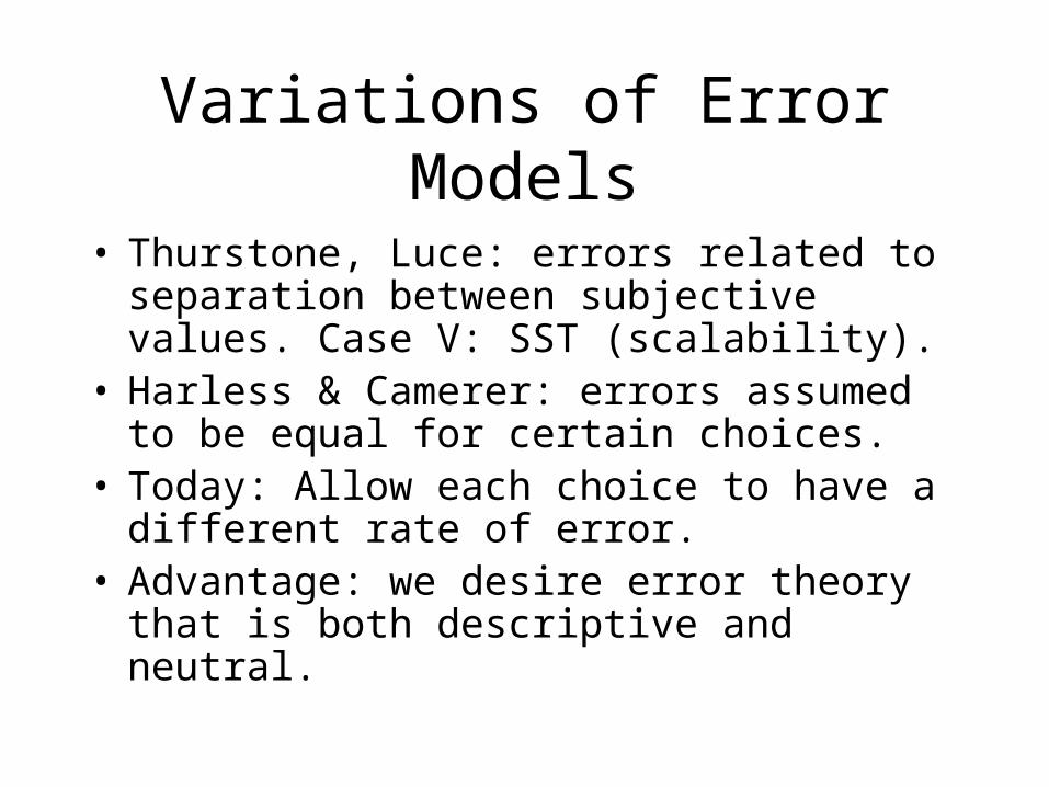
Variations of Error Models

• Thurstone, Luce: errors related to separation between subjective values. Case V: SST (scalability).

• Harless & Camerer: errors assumed to be equal for certain choices.

• Today: Allow each choice to have a different rate of error.

• Advantage: we desire error theory that is both descriptive and neutral.

Basic Assumptions

• Each choice in an experiment has a true choice probability, p, and an error rate, e.

• The error rate is estimated from (and is the “reason” given for) inconsistency of response to the same choice by same person over repetitions

One Choice, Two Repetitions

A B

A

B€

pe2

+ ( 1 − p )( 1 − e )2

p ( 1 − e ) e + ( 1 − p )( 1 − e ) e

p ( 1 − e ) e + ( 1 − p )( 1 − e ) e

€

p ( 1 − e )2

+ ( 1 − p ) e2

Solution for e

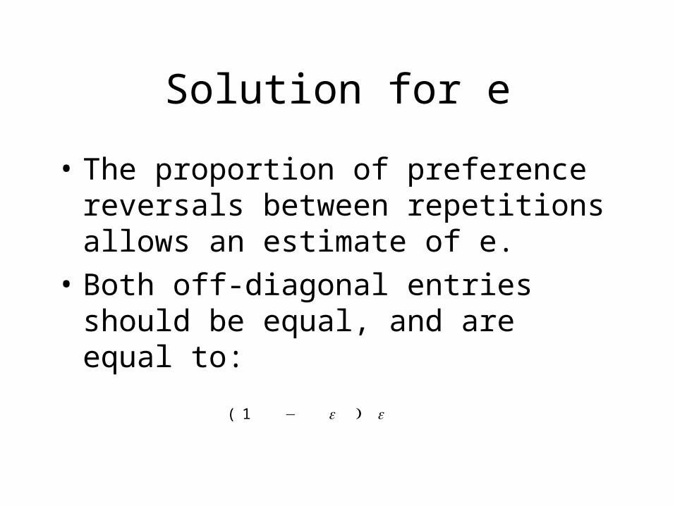
• The proportion of preference reversals between repetitions allows an estimate of e.

• Both off-diagonal entries should be equal, and are equal to:

( 1 − e ) e

Estimating eProbability of Reversals in Repeated Choice

0

0.1

0.2

0.3

0.4

0.5

0 0.1 0.2 0.3 0.4 0.5

Error Rate (e)

Estimating p

Observed = P(1 - e)(1 - e)+(1 - P)ee

0.00

0.20

0.40

0.60

0.80

1.00

0.00 0.20 0.40 0.60 0.80 1.00

True Choice Probabiity, P

Error Rate = 0

Error Rate = .02

Error Rate = .04

Error Rate = .06

Error Rate = .08

Error Rate = .10

Error Rate = .12

Error Rate = .14

Error Rate = .16

Error Rate = .18

Error Rate = .20

Error Rate = .22

Error Rate = .24

Error Rate = .26

Error Rate = .28

Error Rate = .30

Error Rate = .32

Error Rate = .34

Error Rate = .36

Error Rate = .38

Error Rate = .40

Error Rate = .42

Error Rate = .44

Error Rate = .46

Error Rate = .48

Error Rate = .50

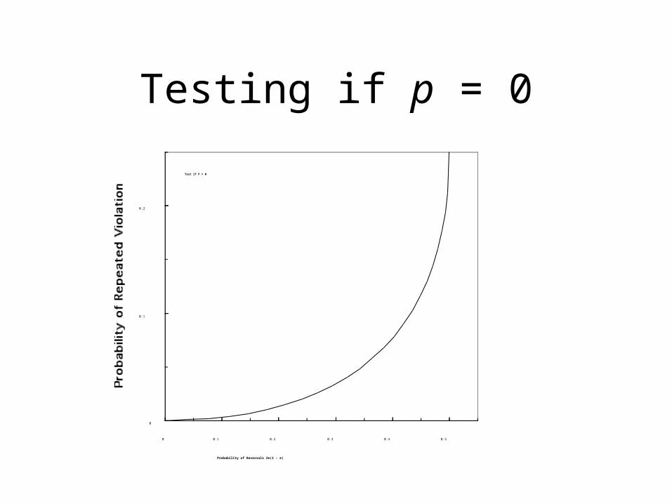
Testing if p = 0

Test if P = 0

0

0.1

0.2

0 0.1 0.2 0.3 0.4 0.5

Probability of Reversals 2e(1 - e)

Ex: Stochastic Dominance

: 05 tickets to win $12

05 tickets to win $14

90 tickets to win $96

B: 10 tickets to win $12

05 tickets to win $90

85 tickets to win $96

122 Undergrads: 59% repeated viols (BB) 28% Preference Reversals (AB or BA) Estimates: e = 0.19; p = 0.85170 Experts: 35% repeated violations 31% Reversals Estimates: e = 0.196; p = 0.50 Chi-Squared test reject H0: p < 0.4

Testing 3-Choice Properties

• Extending this model to properties using 2, 3, or 4 choices is straightforward.

• Allow a different error rate on each choice.

• Allow a true probability for each choice pattern.

Response CombinationsNotation (A, B) (B, C) (C, A)

000 A B C *

001 A B A

010 A C C

011 A C A

100 B B C

101 B B A

110 B C C

111 B C A *

Weak Stochastic Transitivity

€

P ( A f B ) = P ( 000 ) + P ( 001 ) + P ( 010 ) + P ( 011 )

P ( B f C ) = P ( 000 ) + P ( 001 ) + P ( 100 ) + P ( 101 )

P ( C f A ) = P ( 000 ) + P ( 010 ) + P ( 100 ) + P ( 110 )

WST Can be Violated even when Everyone is Perfectly

Transitive

€

P ( 001 ) = P ( 010 ) = P ( 100 ) =1

3

€

P ( A f B ) = P ( B f C ) = P ( C f A ) =2

3

Model for Transitivity

€

P ( 000 ) = p000

( 1 − e1

)( 1 − e2

)( 1 − e3

) + p001

( 1 − e1

)( 1 − e2

) e3

+

+ p010

( 1 − e1

) e2

( 1 − e3

) + p011

( 1 − e1

) e2e

3+

+ p100

e1

( 1 − e2

)( 1 − e3

) + p101

e1

( 1 − e2

) e3

+

+ p110

e1e

2( 1 − e

3) + p

111e

1e

2e

3

A similar expression is written for the other seven probabilities. These can in turn be expanded to predict the probabilities of showing each pattern repeatedly.

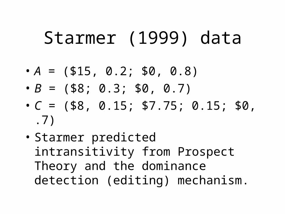
Starmer (1999) data

• A = ($15, 0.2; $0, 0.8)

• B = ($8; 0.3; $0, 0.7)

• C = ($8, 0.15; $7.75; 0.15; $0, .7)

• Starmer predicted intransitivity from Prospect Theory and the dominance detection (editing) mechanism.

Starmer (Best) DataObserved Trans Intrans

Data Fitted (5) Fitted (6)

000 1 2.2 1.2

001 5 4.1 3.7

010 17 22.7 16.8

011 49 43.4 50.1

100 6 4.9 5.6

101 1 2.6 3.6

110 75 81.4 75.2

111 50 42.6 47.9

Transitive Solution to Starmer Data

€

e1

≡ 0

€

e2

= 0 . 06

€

e3

= 0 . 34

€

p010 = 0.01

€

p011 = 0.34; p110 = 0.65

Full model is underdetermined. One error Fixed to zero; but other errors not equal.Most people recognized dominance.

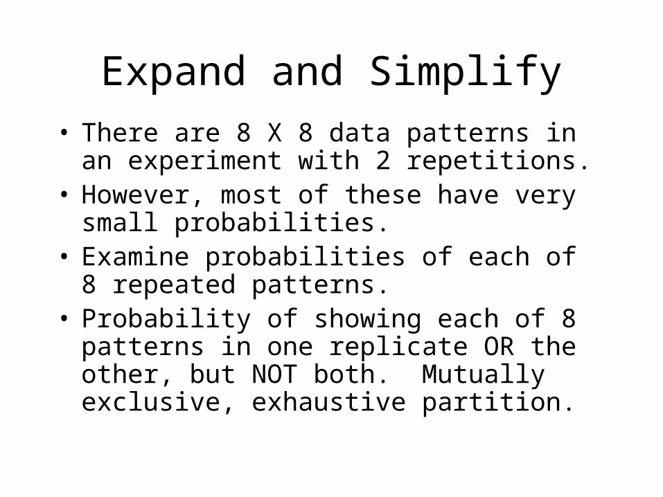
Expand and Simplify• There are 8 X 8 data patterns in an

experiment with 2 repetitions.• However, most of these have very small

probabilities.• Examine probabilities of each of 8

repeated patterns.• Probability of showing each of 8

patterns in one replicate OR the other, but NOT both. Mutually exclusive, exhaustive partition.

New Studies of Transitivity

• Work currently under way testing transitivity under same conditions as used in tests of other decision properties.

• Participants view choices via the WWW, click button beside the gamble they would prefer to play.

Some Recipes being Tested

• Tversky’s (1969) 5 gambles.• LS: Preds of Priority Heuristic• Starmer’s recipe• Additive Difference Model• Birnbaum, Patton, & Lott (1999)

recipe.

Tversky Gambles

• Some Sample Data, using Tversky’s 5 gambles, but formatted with tickets instead of pie charts.

• Data as of May 5, 2005, n = 123.• No pre-selection of participants.• Participants served in other

studies, prior to testing (~1 hr).

Three of the Gambles

• A = ($5.00, 0.29; $0, 0.79)• C = ($4.50, 0.38; $0, 0.62)• E = ($4.00, 0.46; $0, 0.54)

Results-ACEpattern Rep 1 Rep 2 Both

000 10 21 5

001 11 13 9

010 14 23 1

011 7 1 0

100 16 19 4

101 4 3 1

110 176 154 133

111 13 17 3

sum 251 251 156

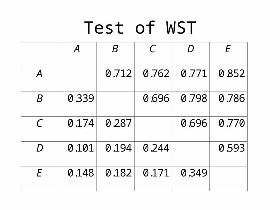
Test of WSTA B C D E

A 0.712 0.762 0.771 0.852

B 0.339 0.696 0.798 0.786

C 0.174 0.287 0.696 0.770

D 0.101 0.194 0.244 0.593

E 0.148 0.182 0.171 0.349

Comments

• Preliminary results were surprisingly transitive.

• Difference: no pre-test, selection• Probability represented by # of

tickets (100 per urn)• Participants have practice with

variety of gambles, & choices.• Tested via Computer

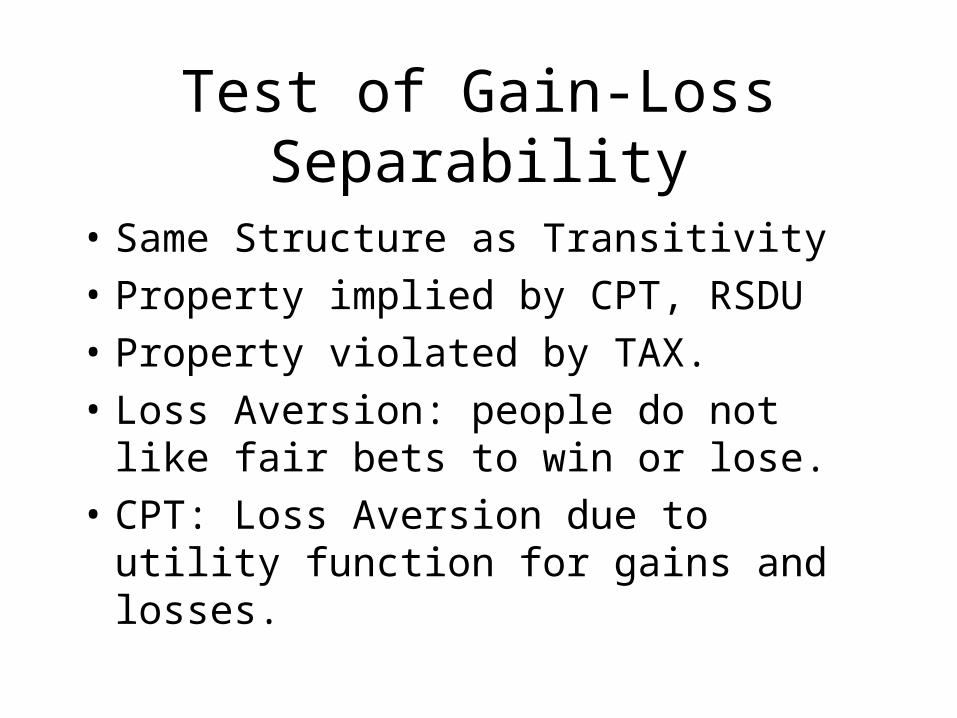
Test of Gain-Loss Separability

• Same Structure as Transitivity• Property implied by CPT, RSDU• Property violated by TAX.• Loss Aversion: people do not like

fair bets to win or lose.• CPT: Loss Aversion due to utility

function for gains and losses.

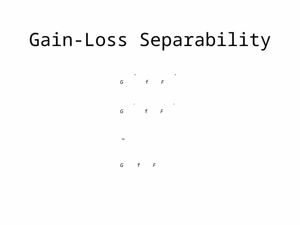
Gain-Loss Separability

€

G

+

f F

+

G

−

f F

−

⇒

G f F

Notation

€

x1

< x2

< K < xn

< 0 ≤ ym

< K y2

< y1

€

G = ( x1

, p1

; x2

, p2

; K ; xn

, pn

; ym

, qm

; K ; y2

, q2

; y1

, q1

)

€

G

+

= ( 0 , pi

i = 1

n

∑ ; ym

, pm

; K ; y2

, q2

; y1

, q1

)

€

G

−

= ( x1

, p1

; x2

, p2

; K ; xn

, pn

; 0 , q

i = 1

m

∑i

)

Birnbaum & Bahra--% FChoice % G Prior TAX Prior CPT

G F G F G F

25 black to win $100

25 white to win $0

50 white to win $0

25 blue to win $50

25 blue to win $50

50 white to win $0

0.71 14 21 25 19

50 white to lose $0

25 pink to lose $50

25 pink to lose $50

50 white to lose $0

25 white to lose $0

25 red to lose $100

0.65 -21 -14 -20 -25

25 black to win $100

25 white to win $0

25 pink to lose $50

25 pink to lose $50

25 blue to win $50

25 blue to win $50

25 white to lose $0

25 red to lose $100

0.52 -25 -25 -9 -15

25 black to win $100

25 white to win $0

50 pink to lose $50

50 blue to win $50

25 white to lose $0

25 red to lose $100

0.24 -15 -34 -9 -15

Birnbaum & BahraR 1 R 2 both OR!- “true”

000 16 17 5 11.5 0.08

001 5 6 0 5.5 0.00

010 24 29 12 14.5 0.18

011 3 5 0 4 0.00

100 36 30 10 23 0.10

101 8 8 1 7 0.00

110 63 54 29 29.5 0.51

111 23 29 9 17 0.13

178 178 66 112 1.00

Summary GLS

• Wu & Markle (2004) found evidence of violation of GLS. Modified CPT.

• Birnbaum & Bahra (2005) also find evidence of violation of GLS, violations of modified CPT as well.

• TAX: In mixed gambles, losses get greater weight. Data do not require kink in the utility function at zero.

Summary

• True & Error model with different error rates seems a reasonable “null” hypothesis for testing transitivity and other properties.

• Requires data with replications so that we can use each person’s self-agreement or reversals to estimate whether response patterns are “real” or due to “error.”