testing wisconsin asphalt mixtures for the aashto 2002 · ii technical report documentation page 1....
TRANSCRIPT

DISCLAIMER
This research was funded through the Wisconsin Highway Research Program by the Wisconsin Department of Transportation and the Federal Highway Administration under Project # 0092-04-07. The contents of this report reflect the views of the authors who are responsible for the facts and the accuracy of the data presented herein. The contents do not necessarily reflect the official views of the Wisconsin Department of Transportation or the Federal Highway Administration at the time of publication. This document is disseminated under the sponsorship of the Department of Transportation in the interest of information exchange. The United States Government assumes no liability for its contents or use thereof. This report does not constitute a standard, specification or regulation. The United States Government does not endorse products or manufacturers. Trade and manufacturers’ names appear in this report only because they are considered essential to the object of the document.

ii
Technical Report Documentation Page 1. Report No. WHRP 07-06
2. Government Accession No
3. Recipient’s Catalog No
4. Title and Subtitle Testing Wisconsin Asphalt Mixtures for the AASHTO 2002 Mechanistic Design Procedure
5. Report Date July 2007
6. Performing Organization Code Univ. of Wisconsin - Madison
7. Authors R. Christopher Williams
8. Performing Organization Report No.
9. Performing Organization Name and Address Department of Civil, Construction and Environmental
Engineering, Iowa State University
10. Work Unit No. (TRAIS)
11. Contract or Grant No. WisDOT SPR# 0092-04-07
12. Sponsoring Agency Name and Address Wisconsin Department of Transportation Division of Business Services Research Coordination Section 4802 Sheboygan Avenue, Room 104 Madison, WI 53707
13. Type of Report and Period Covered
Final Report, 2004-2007
14. Sponsoring Agency Code
15. Supplementary Notes
16. Abstract The intent of this project was to examine typical hot mix asphalt (HMA) pavements that are constructed in the state of Wisconsin. The analysis compares the suggested pavement structures based on the 1972 pavement design guide currently used in Wisconsin and the same ones based on the new Mechanistic-Empirical Pavement Design Guide. In order to develop the pavement structure as outlined by the new Design Guide, the mechanical properties of the HMA layers were measured from 21 field sampled mixtures. These properties include dynamic modulus and flow number, which have been found to be significant predictors of rutting and fatigue by Witczak et al. (2002). Properties of the other layers in the system have been obtained from the Wisconsin Department of Transportation pavement design inputs. The objective was to account for typical construction variability that occurs and to determine its impact upon both mechanical tests. Further, the authors examined these mechanical test results on pavement design to determine if the performance tests and new Design Guide, as they currently exist, are ready for implementation by owners/agencies.
17. Key Words asphalt mixtures—mechanistic-empirical—
pavement design guide—state of Wisconsin
18. Distribution Statement No restriction. This document is available to the public through the National Technical Information Service, 5285 Port Royal Road Springfield, VA 22161
19. Security Classif.(of this report) Unclassified
19. Security Classif. (of this page)
Unclassified
20. No. of Pages
267
21. Price
Form DOT F 1700.7 (8-72) Reproduction of completed page authorized

ii

iii
WISCONSIN HIGHWAY RESEARCH PROGRAM #0092-04-07
TESTING OF WISCONSIN ASPHALT MIXTURES FOR THE
FORTHCOMING AASHTO MECHANISTIC-EMPIRICAL PAVEMENT
DESIGN PROCEDURE
FINAL REPORT
By
R. Christopher Williams, Ph.D. Christopher J. Robinette
Jason Bausano, Ph.D. Tamer Breakah
SUBMITTED TO THE WISCONSIN DEPARTMENT OF TRANSPORTATION
SEPTEMBER 2007

iv

v
ACKNOWLEDGMENTS
The authors would like to acknowledge the support of this project by the Wisconsin Department of Transportation (DOT) and the technical coordination of the Wisconsin Highway Research Program. Specifically, the Wisconsin DOT, the Wisconsin Asphalt Pavement Association (WAPA), and their members are greatly appreciated for assisting in the identification of field projects, sampling assistance, and technical guidance for this project. Lenny Makowski, Laura Fenley, Judie Ryan, and Tom Brokaw at the Wisconsin DOT provided significant assistance in moving this project forward and their efforts are appreciated. The authors would also like to thank Scot Schwandt of WAPA and participating members Erv Dukatz and Signe Erickson from WAPA for work associated with this project. The authors also appreciated the comments and project coordination with the technical oversight committee that Dr. Hani Titi at the University of Wisconsin – Milwaukee provided. The authors would also like to thank the numerous support staff at Michigan Technological University for sample preparation, basic testing and general laboratory operation support, including Ed Tulppo, Jim Vivian, Danielle Ladwig, Michelle Colling, and others. A special thanks to Sabrina Shields-Cook at the Center for Transportation Research and Education at Iowa State University for the substantial editorial review and production of a quality report.

vi

vii
EXECUTIVE SUMMARY
The Wisconsin Department of Transportation (WisDOT) currently uses the AASHTO
1972 Interim Guide for the Design of Pavement Structures for hot mix asphalt. This pavement
design procedure is a strictly empirical pavement design approach; however, with the latest
research and available computer capabilities, mechanistic pavement design procedures have
become more feasible. The new Mechanistic-Empirical Pavement Design Guide and its
associated software have been built on the mechanical properties of the pavement layers while
still using functions to predict pavement life, thus making its approach a mechanistic-empirical
pavement design approach. This pavement design procedure also allows for default values of the
mechanical properties to be used, which are based on previous measurements of these properties.
The intent of this project was to examine typical hot mix asphalt (HMA) pavements that
are constructed in the state of Wisconsin. Projects were sampled throughout the state of
Wisconsin during the 2004 and 2005 construction seasons. Sampling materials from across the
state represented a better cross-section of the materials that were used during the season.
However, most high traffic volume projects were found in the southern regions of Wisconsin,
whereas lower traffic volumes could be found all around the state. This was mainly due to the
population distributions and the location of major trunk lines throughout the state. Sampling was
conducted at the plant site, just after trucks had been loaded out.
The analysis compares the suggested pavement structures based on the 1972 pavement
design guide currently used in Wisconsin and based on the new Design Guide. In order to
develop the pavement structure as outlined by the Design Guide, the mechanical properties of the
HMA layers were measured. These properties include dynamic modulus and flow number, which
have been found to be significant predictors of rutting and fatigue by Witczak et al. (2002).
Properties of the other layers in the system have been obtained from the WisDOT pavement
design inputs. The objective was to account for typical construction variability that occurs and to
determine its impact upon both mechanical tests. Further, the authors examined these mechanical
test results on pavement design to determine if the performance tests and Design Guide as they
currently exist are ready for implementation by owners/agencies.
Chapter 1 of this document provides an introduction to pavement design and the
AASHTO Pavement Design Guide. Chapter 2 discusses past research and studies that have been

viii
conducted that pertain directly to the SuperpaveTM Simple Performance Test (SPT). Included is a
brief description of the research conducted, along with the major findings of the studies that
directly apply to this project. Chapter 3 explains the procedures that were undertaken to sample,
prepare, and test the specimens for this project. Chapter 4 discusses the mixes that were sampled
and some of the difficulties with the original experimental plan. Chapter 5 reviews the specimen
preparation, in terms of the volumetric properties. Chapter 6 presents the results of the SPT
testing of the 21 mixtures from the state of Wisconsin, and Chapter 7 shows the results of the
simulations using the forthcoming AASHTO M-E PDG version 0.800 and compares them to the
1972 AASHTO pavement design guide. Chapter 8 summarizes the conclusions that were
reached. Chapter 9 outlines the recommendations for future work based on the findings of this
project.

ix
LIST OF CONTENTS
Chapter 1. Introduction ................................................................................................................... 1 1.1 Pavement Design Development............................................................................................ 1 1.2 Project Objectives ................................................................................................................. 1 1.3 Overall Project Experimental Plan........................................................................................ 2 1.4 Individual Job Experimental Plan......................................................................................... 4 1.5 Hypotheses for Testing Results ............................................................................................ 5
1.5.1 Dynamic Modulus.......................................................................................................... 5 1.5.2 Flow Number ................................................................................................................. 5 1.5.3 Pavement Structure ........................................................................................................ 6
1.6 Contents of this Document.................................................................................................... 6 Chapter 2. Literature Review.......................................................................................................... 7
2.1 Mechanistic and Mechanistic Empirical Design Approach.................................................. 7 2.2 Mechanistic and Mechanistic-Empirical Pavement Design Development........................... 9 2.3 Development and Design of the Current Mechanistic-Empirical Design Approach...... 15
2.3.1 Previous Barriers to Mechanistic-Empirical Design Implementation ......................... 17 2.3.2 The Current Design Guide ........................................................................................... 18
2.4 SuperpaveTM Simple Performance Test (SPT) ................................................................... 21 2.4.1 Dynamic Modulus Test Setup...................................................................................... 22 2.4.2 Dynamic Modulus Literature Review.......................................................................... 25 2.4.3 Tertiary Flow ............................................................................................................... 29 2.4.4 Repeated Load (Flow Number) Test Setup ................................................................. 29 2.4.5 Repeated Load Test (Flow Number) Literature Review.............................................. 30
2.5 Specimen Geometry............................................................................................................ 34 2.6 Specimen Variability .......................................................................................................... 36 2.7 Test Variability ................................................................................................................... 37 2.8 Volumetric Sensitivity ........................................................................................................ 37
Chapter 3. Procedures ................................................................................................................... 39 3.1 Materials Collection............................................................................................................ 39 3.2 Specimen Preparation and Testing...................................................................................... 39
3.2.1 Splitting........................................................................................................................ 40 3.2.2 Maximum Theoretical Specific Gravity (Gmm)............................................................ 40 3.2.3 Specimen Compaction ................................................................................................. 41 3.2.4 Bulk Specific Gravity (Gmb) ........................................................................................ 41 3.2.5 Specimen Cutting and Coring...................................................................................... 42
3.3 Specimen Measurement ...................................................................................................... 43 3.4 Testing and Calculations..................................................................................................... 43
3.4.1 Dynamic Modulus........................................................................................................ 43 3.4.2 Flow Number ............................................................................................................... 46 3.4.3 Testing Durations......................................................................................................... 48
Chapter 4. Projects sampled.......................................................................................................... 50 4.1 Experimental Plan Changes ................................................................................................ 50 4.2 Sampled Projects................................................................................................................. 51 4.3 Sampling ............................................................................................................................. 52

x
Chapter 5. Sample Preparation ..................................................................................................... 56 5.1 Sample Preparation Flowchart ............................................................................................ 56 5.2 Maximum Theoretical Specific Gravity ............................................................................. 57 5.3 Compaction ......................................................................................................................... 61 5.4 Bulk Specific Gravity of Gyratory...................................................................................... 62 5.5 Volumetrics of Sawed/Cored Test Specimens.................................................................... 64
Chapter 6. Wisconsin Mix Testing ............................................................................................... 65 6.1 Jobs Tested.......................................................................................................................... 65 6.2 Dynamic Modulus Loading Stress...................................................................................... 65 6.3 Dynamic Modulus and Dynamic Creep Test Results ......................................................... 66
6.3.1 Brule............................................................................................................................. 67 6.3.2 Baraboo ........................................................................................................................ 67 6.3.3 Hurley .......................................................................................................................... 68 6.3.4 Cascade ........................................................................................................................ 68 6.3.5 Bloomville.................................................................................................................... 69 6.3.6 Medford........................................................................................................................ 69 6.3.7 Wautoma...................................................................................................................... 70 6.3.8 Tomahawk.................................................................................................................... 70 6.3.9 Waunakee..................................................................................................................... 71 6.3.10 Mosinee...................................................................................................................... 71 6.3.11 Cumberland................................................................................................................ 72 6.3.12 Hayward..................................................................................................................... 72 6.3.13 Wausau....................................................................................................................... 73 6.3.14 Hurley ........................................................................................................................ 73 6.3.15 Antigo ........................................................................................................................ 74 6.3.16 Northfield................................................................................................................... 74 6.3.17 Wisconsin Rapids....................................................................................................... 75 6.3.18 Antigo ........................................................................................................................ 75 6.3.19 Plymouth .................................................................................................................... 76 6.3.20 Racine ........................................................................................................................ 76 6.3.21 Northfield................................................................................................................... 77 6.3.22 Pooled Data for Database........................................................................................... 77 6.3.23 Statistical Analysis..................................................................................................... 83
Chapter 7. AASHTO M-E PDG Simulations ............................................................................... 94 7.1 Pavement Design ................................................................................................................ 94
7.1.1 Brule............................................................................................................................. 95 7.1.2 Baraboo ........................................................................................................................ 99 7.1.3 Hurley ........................................................................................................................ 104 7.1.4 Cascade ...................................................................................................................... 109 7.1.5 Bloomville.................................................................................................................. 113 7.1.6 Medford...................................................................................................................... 117 7.1.7 Wautoma.................................................................................................................... 121 7.1.8 Tomahawk.................................................................................................................. 126 7.1.9 Waunakee................................................................................................................... 130 7.1.10 Mosinee.................................................................................................................... 135 7.1.11 Cumberland.............................................................................................................. 139

xi
7.1.12 Hayward................................................................................................................... 144 7.1.13 Wausau..................................................................................................................... 149 7.1.14 Hurley ...................................................................................................................... 154 7.1.15 Antigo ...................................................................................................................... 159 7.1.16 Northfield................................................................................................................. 163 7.1.17 Wisconsin Rapids..................................................................................................... 167 7.1.18 Plymouth .................................................................................................................. 172 7.1.19 Racine ...................................................................................................................... 176 7.1.20 WisPave Results....................................................................................................... 180 7.1.21 Comparison of M-E PDG versus WisPave.............................................................. 181
Chapter 8. Conclusions ............................................................................................................... 185 Chapter 9. Recommendations ..................................................................................................... 187 APPENDIX A. Project JMFs...................................................................................................... A-1 APPENDIX B. Specimen Volumetrics Before Sawing/Coring ................................................. B-1 APPENDIX C. Specimen Volumetrics After Sawing/Coring.................................................... C-1

xii

xiii
LIST OF FIGURES
Figure 2.1. n-Layered system (Huang 2003) .................................................................................. 8 Figure 2.2. Mechanical models: (a) Maxwell, (b) Kelvin-Voigt, and (c) Burger......................... 12 Figure 2.3. Viscoelastoplastic component model (Lytton et al, 1993) ......................................... 13 Figure 2.4. Dynamic modulus loading.......................................................................................... 23 Figure 2.5. Flow number loading.................................................................................................. 30 Figure 3.1. Changes in weight of specimen after Gmb determination ........................................... 42 Figure 4.1. Project locations (prepared by Demographic Services Center, Wisconsin Department
of Administration and the Wisconsin State Cartographer’s Office) .......................................... 52 Figure 4.2. Truck being loaded out............................................................................................... 53 Figure 4.3. Sampling rack............................................................................................................. 54 Figure 4.4. HMA sampling ........................................................................................................... 54 Figure 4.5. Stockpile cone proportions ......................................................................................... 55 Figure 5.1. Sample preparation flow chart.................................................................................... 56 Figure 5.2. MTU and contractor Gmm optimum asphalt binder content ....................................... 59 Figure 5.3. MTU and contractor Gmm +0.3% optimum asphalt binder content............................ 60 Figure 5.4. Prepared gyratory specimens...................................................................................... 62 Figure 7.1. Brule permanent deformation in AC layer ................................................................. 97 Figure 7.2. Brule permanent deformation in total pavement ........................................................ 97 Figure 7.3. Brule IRI..................................................................................................................... 98 Figure 7.4. Brule longitudinal cracking ........................................................................................ 98 Figure 7.5. Brule alligator cracking .............................................................................................. 99 Figure 7.6. Baraboo permanent deformation in AC layer .......................................................... 101 Figure 7.7. Baraboo permanent deformation in total pavement ................................................. 101 Figure 7.8. Baraboo IRI .............................................................................................................. 102 Figure 7.9. Baraboo longitudinal cracking ................................................................................. 102 Figure 7.10. Baraboo alligator cracking ..................................................................................... 103 Figure 7.11. Hurley permanent deformation in AC layer ........................................................... 106 Figure 7.12. Hurley permanent deformation in total pavement.................................................. 106 Figure 7.13. Hurley IRI............................................................................................................... 107 Figure 7.14. Hurley longitudinal cracking.................................................................................. 107 Figure 7.15. Hurley alligator cracking........................................................................................ 108 Figure 7.16. Cascade permanent deformation in AC layer......................................................... 110 Figure 7.17. Cascade permanent deformation in total pavement................................................ 111 Figure 7.18. Cascade IRI ............................................................................................................ 111 Figure 7.19. Cascade longitudinal cracking................................................................................ 112 Figure 7.20. Cascade alligator cracking...................................................................................... 112 Figure 7.21. Bloomville permanent deformation in AC layer .................................................... 115 Figure 7.22. Bloomville permanent deformation in total pavement........................................... 115 Figure 7.23. Bloomville IRI........................................................................................................ 116 Figure 7.24. Bloomville longitudinal cracking ........................................................................... 116 Figure 7.25. Bloomville alligator cracking ................................................................................. 117 Figure 7.26. Medford permanent deformation in AC layer ........................................................ 119 Figure 7.27. Medford permanent deformation in total pavement............................................... 119

xiv
Figure 7.28. Medford IRI............................................................................................................ 120 Figure 7.29. Medford longitudinal cracking ............................................................................... 120 Figure 7.30. Medford alligator cracking ..................................................................................... 121 Figure 7.31. Wautoma permanent deformation in AC layer ...................................................... 123 Figure 7.32. Wautoma permanent deformation in total pavement ............................................. 123 Figure 7.33. Wautoma IRI .......................................................................................................... 124 Figure 7.34. Wautoma longitudinal cracking ............................................................................. 124 Figure 7.35. Wautoma alligator cracking ................................................................................... 125 Figure 7.36. Tomahawk permanent deformation in AC layer .................................................... 127 Figure 7.37. Tomahawk permanent deformation in total pavement........................................... 128 Figure 7.38. Tomahawk IRI........................................................................................................ 128 Figure 7.39. Tomahawk longitudinal cracking ........................................................................... 129 Figure 7.40. Tomahawk alligator cracking ................................................................................. 129 Figure 7.41. Waunakee permanent deformation in AC layer ..................................................... 132 Figure 7.42. Waunakee permanent deformation in total pavement ............................................ 132 Figure 7.43. Waunakee IRI......................................................................................................... 133 Figure 7.44. Waunakee longitudinal cracking ............................................................................ 133 Figure 7.45. Waunakee alligator cracking .................................................................................. 134 Figure 7.46. Mosinee permanent deformation in AC layer ........................................................ 137 Figure 7.47. Mosinee permanent deformation in total pavement ............................................... 137 Figure 7.48. Mosinee IRI ............................................................................................................ 138 Figure 7.49. Mosinee longitudinal cracking ............................................................................... 138 Figure 7.50. Mosinee alligator cracking ..................................................................................... 139 Figure 7.51. Cumberland permanent deformation in AC layer .................................................. 141 Figure 7.52. Cumberland permanent deformation in total pavement ......................................... 142 Figure 7.53. Cumberland IRI ...................................................................................................... 142 Figure 7.54. Cumberland longitudinal cracking ......................................................................... 143 Figure 7.55. Cumberland alligator cracking ............................................................................... 143 Figure 7.56. Hayward permanent deformation in AC layer ....................................................... 146 Figure 7.57. Hayward permanent deformation in total pavement .............................................. 146 Figure 7.58. Hayward IRI ........................................................................................................... 147 Figure 7.59. Hayward longitudinal lracking ............................................................................... 147 Figure 7.60. Hayward alligator cracking .................................................................................... 148 Figure 7.61. Wausau permanent deformation in AC layer ......................................................... 151 Figure 7.62. Wausau permanent deformation in total pavement ................................................ 151 Figure 7.63. Wausau IRI............................................................................................................. 152 Figure 7.64. Wausau longitudinal cracking ................................................................................ 152 Figure 7.65. Wausau alligator cracking ...................................................................................... 153 Figure 7.66. Hurley permanent deformation in AC layer ........................................................... 156 Figure 7.67. Hurley permanent deformation in total pavement.................................................. 156 Figure 7.68. Hurley IRI............................................................................................................... 157 Figure 7.69. Hurley longitudinal cracking.................................................................................. 157 Figure 7.70. Hurley alligator cracking........................................................................................ 158 Figure 7.71. Antigo permanent deformation in AC layer ........................................................... 160 Figure 7.72. Antigo permanent deformation in total pavement.................................................. 161 Figure 7.73. Antigo IRI............................................................................................................... 161

xv
Figure 7.74. Antigo longitudinal cracking.................................................................................. 162 Figure 7.75. Antigo alligator cracking........................................................................................ 162 Figure 7.76. Northfield permanent deformation in AC layer ..................................................... 165 Figure 7.77. Northfield permanent deformation in total pavement ............................................ 165 Figure 7.78. Northfield IRI ......................................................................................................... 166 Figure 7.79. Northfield longitudinal cracking ............................................................................ 166 Figure 7.80. Northfield alligator cracking .................................................................................. 167 Figure 7.81. Wisconsin Rapids permanent deformation in AC layer ......................................... 169 Figure 7.82. Wisconsin Rapids permanent deformation in total pavement................................ 170 Figure 7.83. Wisconsin Rapids IRI............................................................................................. 170 Figure 7.84. Wisconsin Rapids longitudinal cracking ................................................................ 171 Figure 7.85. Wisconsin Rapids alligator cracking ...................................................................... 171 Figure 7.86. Plymouth permanent deformation in AC layer ...................................................... 173 Figure 7.87. Plymouth permanent deformation in total pavement ............................................. 174 Figure 7.88. Plymouth IRI .......................................................................................................... 174 Figure 7.89. Plymouth longitudinal cracking ............................................................................. 175 Figure 7.90. Plymouth alligator cracking ................................................................................... 175 Figure 7.91. Racine permanent deformation in AC layer ........................................................... 177 Figure 7.92. Racine permanent deformation in total pavement.................................................. 178 Figure 7.93. Racine IRI............................................................................................................... 178 Figure 7.94. Racine longitudinal cracking.................................................................................. 179 Figure 7.95. Racine alligator cracking........................................................................................ 179 Figure 7.96. WisPave results for as-builts .................................................................................. 181

xvi

xvii
LIST OF TABLES
Table 1.1. Preliminary experimental matrix for field sampling...................................................... 3 Table 1.2. Experimental plan for volumetric changes .................................................................... 4 Table 2.1. SPT advantages and disadvantages (NCHRP Report 465 2002 and NCAT Report 01-
05) .............................................................................................................................................. 22 Table 2.2. Uniaxial data analysis (Witczak et al. 2000) ............................................................... 35 Table 3.1. Dynamic modulus testing configurations .................................................................... 44 Table 3.2. Cycles for test sequence............................................................................................... 44 Table 3.3. Durations for SSPT preparation and testing (NCHRP 465, 2002b) ............................ 49 Table 4.1. Revised project matrix ................................................................................................. 50 Table 5.1. Gmm Mean and standard deviation for each project ..................................................... 58 Table 6.1. Dynamic modulus and creep testing for the Brule mixture ......................................... 67 Table 6.2. Dynamic modulus and creep testing for the Baraboo mixture .................................... 67 Table 6.3. Dynamic modulus and creep testing for the Hurley mixture....................................... 68 Table 6.4. Dynamic modulus and creep testing for the Cascade mixture..................................... 68 Table 6.5. Dynamic modulus and creep testing for the Bloomville mixture................................ 69 Table 6.6. Dynamic modulus and creep testing for the Medford mixture.................................... 69 Table 6.7. Dynamic modulus and creep testing for the Wautoma mixture .................................. 70 Table 6.8. Dynamic modulus and creep testing for the Tomahawk mixture................................ 70 Table 6.9. Dynamic modulus and creep testing for the Waunakee mixture ................................. 71 Table 6.10. Dynamic modulus and creep testing for the Mosinee mixture .................................. 71 Table 6.11. Dynamic modulus and creep testing for the Cumberland mixture ............................ 72 Table 6.12. Dynamic modulus and creep testing for the Hayward mixture ................................. 72 Table 6.13. Dynamic modulus and creep testing for the Wausau mixture ................................... 73 Table 6.14. Dynamic modulus and creep testing for the Hurley mixture..................................... 73 Table 6.15. Dynamic modulus and creep testing for the Antigo mixture..................................... 74 Table 6.16. Dynamic modulus and creep testing for the Northfield mixture ............................... 74 Table 6.17. Dynamic modulus and creep testing for the Wisconsin Rapids mixture................... 75 Table 6.18. Dynamic modulus and creep testing for the Antigo mixture..................................... 75 Table 6.19. Dynamic modulus and creep testing for the Plymouth mixture ................................ 76 Table 6.20 Dynamic modulus and creep testing for the Racine mixture...................................... 76 Table 6.21. Dynamic modulus and creep testing for the Northfield mixture ............................... 77 Table 6.22. Pooled dynamic modulus and creep testing for dense-graded mixture with an NMAS
of 19.0 mm and 300,000 ESAL traffic level.............................................................................. 77 Table 6.23. Pooled dynamic modulus and creep testing for dense-graded mixture with an NMAS
of 12.5 mm and 300,000 ESAL traffic level.............................................................................. 78 Table 6.24. Pooled dynamic modulus and creep testing for dense-graded mixture with an NMAS
of 19.0 mm and 1,000,000 ESAL traffic level........................................................................... 78 Table 6.25. Pooled dynamic modulus and creep testing for dense-graded mixture with an NMAS
of 12.5 mm and 1,000,000 ESAL traffic level........................................................................... 79 Table 6.26. Pooled dynamic modulus and creep testing for open-graded mixture with an NMAS
of 25.0 mm and 3,000,000 ESAL traffic level........................................................................... 79 Table 6.27. Pooled dynamic modulus and creep testing for dense-graded mixture with an NMAS
of 19.0 mm and 3,000,000 ESAL traffic level........................................................................... 80

xviii
Table 6.28. Pooled dynamic modulus and creep testing for dense-graded mixture with an NMAS of 12.5 mm and 3,000,000 ESAL traffic level........................................................................... 80
Table 6.29. Pooled dynamic modulus and creep testing for dense-graded mixture with an NMAS of 19.0 mm and >3,000,000 ESAL traffic level ........................................................................ 81
Table 6.30. Pooled dynamic modulus and creep testing for open-graded mixture with an NMAS of 19.0 mm and >3,000,000 ESAL traffic level ........................................................................ 81
Table 6.31. Pooled dynamic modulus and creep testing for dense-graded mixture with an NMAS of 12.5 mm and >3,000,000 ESAL traffic level ........................................................................ 82
Table 6.32. Pooled dynamic modulus and creep testing for open-graded mixture with an NMAS of 12.5 mm and >3,000,000 ESAL traffic level ........................................................................ 82
Table 6.33. GLM and LSD results for flow number test results................................................... 84 Table 6.34. GLM and LSD results for accumulated microstrain at flow number test results ...... 85 Table 6.35. GLM and LSD results for E* test results at intermediate temperature and 0.1 Hz ... 86 Table 6.36. GLM and LSD results for E* test results at intermediate temperature and 1.0 Hz ... 87 Table 6.37. GLM and LSD results for E* test results at intermediate temperature and 10.0 Hz . 88 Table 6.38. GLM and LSD results for E* test results at intermediate temperature and 25.0 Hz . 89 Table 6.39. GLM and LSD results for E* test results at high temperature and 0.1 Hz ................ 90 Table 6.40. GLM and LSD results for E* test results at high temperature and 1.0 Hz ................ 91 Table 6.41. GLM and LSD results for E* test results at high temperature and 10.0 Hz .............. 92 Table 6.42. GLM and LSD results for E* test results at high temperature and 25.0 Hz .............. 93 Table 7.1. Design guide software performance criteria ................................................................ 94 Table 7.2. Traffic characteristics—Brule E-0.3 19.0-mm ............................................................ 95 Table 7.3. Traffic characteristics—Baraboo E-0.3 12.5 mm...................................................... 100 Table 7.4. Traffic characteristics—Hurley E-0.3 12.5 mm ........................................................ 105 Table 7.5. Traffic characteristics—Cascade E-1 19.0 mm ......................................................... 109 Table 7.6. Traffic characteristics—Bloomville E-1 19.0 mm .................................................... 114 Table 7.7. Traffic characteristics—Medford E-1 12.5 mm ........................................................ 118 Table 7.8. Traffic characteristics—Wautoma E-1 12.5 mm....................................................... 122 Table 7.9. Traffic characteristics—Tomahawk E-3 25.0 mm .................................................... 126 Table 7.10. Traffic characteristics—Waunakee E-3 19.0 mm.................................................... 131 Table 7.11. Traffic characteristics—Mosinee E-3 19.0 mm....................................................... 136 Table 7.12. Traffic characteristics—Cumberland E-3 19.0-mm ................................................ 140 Table 7.13. Traffic characteristics—Hayward E-3 12.5 mm...................................................... 145 Table 7.14. Traffic characteristics—Wausau E-3 12.5 mm........................................................ 150 Table 7.15. Traffic characteristics—Hurley E-3 12.5 mm ......................................................... 155 Table 7.16. Traffic characteristics—Antigo E-10 12.5 and 19.0 mm......................................... 159 Table 7.17. Traffic characteristics— Northfield E-30 19.0mm.................................................. 164 Table 7.18. Traffic characteristics—Wisconsin Rapids E-10 19.0 mm ..................................... 168 Table 7.19. Traffic characteristics—Plymouth E-10 12.5 mm................................................... 172 Table 7.20. Traffic characteristics—Bloomville E-1 19.0 mm .................................................. 176 Table 7.21. As-built design using 7% air voids at optimum AC using Level 1 design.............. 182 Table 7.22. As-built design using 4% air voids at optimum AC using Level 1 design.............. 183 Table 7.23. As-built design using 10% air voids at optimum AC using Level 1 design............ 183 Table 7.24. As-built design using 7% air voids at 0.3% plus optimum AC using Level 1 design..................................................................................................................................................... 184

xix
ACRONYMS AND SYMBOLS
2D A heavy single unit truck with two axles and 6 tires
3SU A heavy single unit truck with three axles
2S-1 A heavy tractor-semitrailer truck with three axles
2S-2 A heavy tractor-semitrailer with four axles
3S-2 A heavy tractor-semitrailer with five or more axles
2-S1-2 A heavy tractor-semitrailer-trailer combination with five or more axles
A Witczak Predictive Equation Regression Intercept
AADT Average Annual Daily Traffic
AADTT Average Annual Daily Truck Traffic
AASHO American Association of State Highway Officials
AASHTO American Association of State and Highway Transportation Officials
ALF Accelerated Loading Facility
AMS Accumulated Microstrain at Flow Number
ASTM American Society for Testing and Materials
BSG (Gmb) Bulk Specific Gravity
COV Coefficient of Variation
D60 Grain size that corresponds to 60 percent passing
E* and *E Complex Modulus and Dynamic Modulus, respectively
E’ and E” Elastic and Viscous Modulus, respectively
ESAL Equivalent Single Axle Load
FHWA Federal Highway Administration
FN Flow Number
F/Pb Fines to Asphalt Binder Ratio
Gb Asphalt Specific Gravity
Gsb Aggregate Bulk Specific Gravity
Gse Aggregate Effective Specific Gravity
HMA Hot Mix Asphalt
IDT Indirect Tension Test
IRI International Ride Index
JMF Job Mix Formula
JTFP Joint Task Force for Pavements
LTPP Long Term Pavement Performance
LVDT Linear Variable Differential Transducer
M-E Mechanistic-Empirical
MTSG (Gmm) Maximum Theoretical Specific Gravity
MTU Michigan Technological University
NCAT National Center for Asphalt Technology
NCHRP National Cooperative Highway Research Program
Ndesign Design number of gyrations for a SuperpaveTM Mix Design
NMAS Nominal Maximum Aggregate Size
Pb Asphalt Binder Content

xx
Peff Effective Asphalt Binder Content
PI Plasticity Index
PTF Pavement Testing Facility
QC/QA Quality Control/Quality Assurance
R2 Coefficient of Determination
RAP Recycled Asphalt Pavement
RTFO Rolling Thin Film Oven
SGC SuperpaveTM Gyratory Compactor
SHRP Strategic Highway Research Program
SMA Stone Matrix Asphalt
SSD Saturate Surface Dry
SPS Special Pavement Study
SPT Simple Performance Test
SST SuperpaveTM Shear Tester
TAI The Asphalt Institute
TOC Technical Oversight Committee
UTM Universal Testing Machine
V Witczak Predictive Equation Regression Slope
VFA Voids Filled with Asphalt
VMA Voids in the Mineral Aggregate
WHRP Wisconsin Highway Research Program
WisDOT Wisconsin Department of Transportation
WSDOT Washington Department of Transportation
εεεεo Strain
φφφφ Phase Angle
σσσσo Stress

1
CHAPTER 1. INTRODUCTION
1.1 Pavement Design Development
The American Association of State Highway Officials (AASHO) Road Test in the late
1950s formed the basic principles for flexible pavement design in the United States. The
AASHO Road Test was meant to identify relationships between the loading magnitude and
arrangement as well as between pavement thickness and performance. Based on the results of the
Road Test, empirical relationships were developed that made the pavement design process
relatively simplistic. Some of the basic inputs include a soil support value, pavement loading,
and a regional factor, used to develop a structural number for a layer and ultimately a layer
thickness (Washington DOT Manual 1995). This procedure is outlined in the 1972 American
Association of State Highway and Transportation Officials (AASHTO) Interim Guide for Design
of Pavement Structures. There have been continual revisions to the initial design guide, leading
to the development of the AASHTO Guide for Design of New and Rehabilitated Pavement
Structures (Design Guide), which is the culmination of research and field experience. The newest
Design Guide is based on a mechanistic-empirical (M-E) design approach and has been put
together under the auspices of the National Cooperative Highway Research Program (NCHRP)
as projects 1-37, 1-37A, 1-40A & B, 9-19, and 9-29 (Guide for Mechanistic-Empirical Design of
New and Rehabilitated Pavement Structures 2004).
1.2 Project Objectives
The Wisconsin Department of Transportation (WisDOT) currently uses the AASHTO
1972 Interim Guide for the Design of Pavement Structures for hot mix asphalt. This pavement
design procedure is a strictly empirical pavement design approach; however, with the latest
research and available computer capabilities, mechanistic pavement design procedures have
become more feasible. The Design Guide and its associated software have been built on the
mechanical properties of the pavement layers while still using functions to predict pavement life,
thus making its approach a mechanistic-empirical pavement design approach. This pavement
design procedure also allows for default values of the mechanical properties to be used, which
are based on previous measurements of these properties.

2
The intent of this project was to examine typical hot mix asphalt (HMA) pavements that
are constructed in the state of Wisconsin. The analysis compares the suggested pavement
structures based on the 1972 pavement design guide currently used in Wisconsin and based on
the new Design Guide. In order to develop the pavement structure as outlined by the Design
Guide the mechanical properties of the HMA layers were measured. These properties include
dynamic modulus and flow number, which have been found to be significant predictors of rutting
and fatigue by Witczak et al. (2002). Properties of the other layers in the system have been
obtained from the WisDOT pavement design inputs. The objective was to account for typical
construction variability that occurs and to determine its impact upon both mechanical tests.
Further, the authors examined these mechanical test results on pavement design to determine if
the performance tests and Design Guide as they currently exist are ready for implementation by
owners/agencies.
1.3 Overall Project Experimental Plan
The first step in developing the experimental plan was to identify HMA designs that have
realistic construction parameters. The pavements should be representative of HMA designs used
in practice by owners/agencies. Predominate factors that have been identified in the mix design
process are (1) the level of anticipated traffic, (2) the nominal maximum aggregate size (NMAS),
and (3) mix type (dense- or open-graded).
In this research plan, the level of traffic had been initially segmented into three categories
by equivalent single axle loads (ESAL), which corresponds to an 18,000-lb axle load. Low
volume traffic levels were considered to have less than or equal to 1x10⁶ ESALs. Medium
volume traffic levels were greater than 1x10⁶ ESALs up to 3x10⁶ ESALs. Finally, high volume
traffic levels were greater than 3x10⁶ ESALs. The reason for this segmentation is that the level of
anticipated traffic is a critical variable in the pavement design process that ultimately results in
aggregate angularity and thickness recommendations. Changes in pavement thickness can
significantly affect the amount of rutting that occurs in the pavement structure and, consequently,
has been noted as one of the variables important in the experimental matrix.
The second factor that was considered was the nominal maximum aggregate size
(NMAS). The sizes that were considered are as follows: 25.0-mm, 19.0-mm, and 12.5-mm. As

3
noted by Akhter and Witczak (1985), the size of the aggregate plays a significant role in
permanent deformation.
The type of mix was also analyzed in terms of dense- and open-graded and is a function
of the gradation. A Stone Matrix Asphalt (SMA) will be considered an open-graded mix for this
project. A SMA promotes stone-on-stone contact by having highly crushed material, with a
higher fines content and added fibers. SMAs have been utilized in Europe for many years and
were introduced to the United States in 1991 (Brown 1997). As part of Brown’s study, it was
observed that 31 SMA projects had been paved in the U.S. between 1991 and 1993. This is not to
say that SMA projects have not been paved after this time frame—they have—but it points to the
increased utilization of this type of mix design. As a result of this higher utilization, the SMA
mix type has been included in this study for the high traffic level pavements, where it is intended
to mitigate permanent deformation. It should be noted that owners/agencies predominately pave
dense-graded mixes, with open-graded mixes used only on high volume roads; this has been
factored into the experimental matrix found in Table 1.1.
Table 1.1. Preliminary experimental matrix for field sampling
Traffic level Nominal
maximum
aggregate size
Mix type Low Medium High
Dense X1 XXX 25.0mm
Open
Dense X XXX X 19.0mm
Open X
Dense XXX XXX XXX 12.5mm
Open X 1An X denotes a single mix.
This plan directly emphasizes low and medium volume roads because these represent the
majority of the roadway miles an owner/agency maintains and, hence, the greatest number of
mix designs performed annually. However, the high volume roadways have the greatest vehicle-
miles traveled in the state, making them more prone to failure by permanent deformation; thus,
these mixes have been included as well.

4
1.4 Individual Job Experimental Plan
For each job, a replicate experimental plan that examines the effects of changes in air
voids and asphalt binder content has been developed. The reason for this portion of the research
project was to understand variations that typically occur during field production. Depending on
the ease of compaction and the temperature of the mat, the in-situ air voids after initial
construction can vary significantly. This variability can significantly affect pavement
performance. Contractors will typically seek 92.0% Gmm, or 8.0% air voids, so that they can
receive full pay for a job in Wisconsin. However, this may not always be achievable and thus
higher air void contents were examined (Wisconsin Construction Specification 2004).
In terms of the asphalt content, the contractors are allowed to deviate ±0.3% from that of
the asphalt content stipulated in the accepted job mix formula (JMF), which was stated in Section
460.2.8.2.1.5 of the Wisconsin Constructions Specifications (2004) and is typical of most
owners/agencies. It should be noted that since mixes were being sampled from field produced
mixes being placed on roadways, testing at a lower asphalt binder content than that produced was
not possible. This portion of the experimental plan can be found in Table 1.2.
Table 1.2. Experimental plan for volumetric changes
Asphalt binder content
Sampled (assumed
optimum) Sampled + 0.3%
Low X1 N/T2
Target X X
Air voids (compaction effort) High X N/T
1 An X denotes six specimens for each project.
2 N/T denotes not tested.
Changes in air voids were obtained through changing the weight of mix in the specimen
and compacting to a given height of 170.0-mm. Low, target, and high refer to 4.0, 7.0, and
10.0% air voids, respectively. Testing was also carried out with specimens in which the asphalt
binder content was increased 0.3% by weight of the mix. This material necessitated further
mixing. The extra asphalt binder was sampled from the plant where the mixture was produced.
The procedures for sample procurement and preparation for testing are outlined in Chapter 3.

5
1.5 Hypotheses for Testing Results
Based on past testing and research from the literature review, hypotheses were developed
regarding the factors considered in the experimental plan. The statistical analyses of these
hypotheses are presented in Chapter 6. These hypotheses are outlined in the following sections
for dynamic modulus, flow number, and pavement design.
1.5.1 Dynamic Modulus
Following are the relationships that are expected to be observed from dynamic modulus
testing and developed prior to the use of SuperpaveTM Simple Performance Test (SPT).
• As temperature increases, dynamic modulus will decrease and phase angle will
increase.
• As air voids increase and likewise compaction effort decreases, dynamic modulus
will decrease.
• As the asphalt cement content increases, dynamic modulus will decrease.
• As the aggregate angularity (corresponding with traffic volume) increases, dynamic
modulus will increase.
1.5.2 Flow Number
The following relationships that are expected to be observed from flow number testing
and developed prior to the use of SuperpaveTM SPT.
• As air voids increases, the flow number will decrease.
• As the asphalt cement content increases, the flow number will decrease.
• As the aggregate angularity (corresponding with traffic volume) increases, the flow
number will increase.

6
1.5.3 Pavement Structure
It is expected that the mechanistic-empirical pavement design would yield a slightly
thinner HMA layer than compared to that of the solely empirical pavement design procedure.
The reason being is that the empirical pavement design has a greater factor of safety built into
the model than mechanistic-empirical pavement design. Minimal distresses would be indicative
of thinner layer thicknesses. The current Design Guide software is more of a design check as
opposed to a design guide. The analysis approach was to input varying thicknesses for the layer
in question with the pavement structure remaining constant and the level of distress through
simulations conducted with the Design Guide software.
1.6 Contents of this Document
Chapter 2 of this document discusses past research and studies that have been conducted
that pertain directly to the SuperpaveTM SPT. Included is a brief description of the research
conducted, along with the major findings of the studies that directly apply to this project. Chapter
3 explains the procedures that were undertaken to sample, prepare, and test the specimens for
this project. Chapter 4 discusses the mixes that were sampled and some of the difficulties with
the original experimental plan. Chapter 5 reviews the specimen preparation, in terms of the
volumetric properties. Chapter 6 presents the results of the SPT testing of the 21 mixtures from
the state of Wisconsin, and Chapter 7 shows the results of the simulations using the forthcoming
AASHTO M-E PDG version 0.800 and compares them to the 1972 AASHTO pavement design
guide. Chapter 8 summarizes the conclusions that were reached. Chapter 9 outlines the
recommendations for future work based on the findings of this project.

7
CHAPTER 2. LITERATURE REVIEW
2.1 Mechanistic and Mechanistic Empirical Design Approach
In 1885, Joseph Boussinesq developed a method for determining induced stresses and
strains in an infinite elastic half-space based on a point load (Coduto 1999). These equations
were based on a linear elastic material and have been applied to asphalt pavements. Asphalt
pavement mixtures have been around since 1874 (Roberts 2002), with informal pavement design
procedures starting to be developed in 1920 (Vesic 1964). These early pavement design
procedures were based primarily on “rules of thumb,” as well as past experience. Burmister
(1943) appears to be the first researcher to apply a mechanistic analysis to a multi-layer system
for the purposes of pavement design. A considerable amount of work has been conducted since
Burmister, which has ultimately led to the development of the current AASHTO Design Guide
for New and Rehabilitated Pavements, henceforth referred to as the Design Guide.
A mechanistic pavement design utilizes mechanical modeling to determine the stress,
strain, and displacement under a load (Timm 1998) and, more importantly, a wheel load. With
knowledge of the various layer properties (which depends on the method of analysis) of the
pavement structure, these reactions can be determined and incorporated into empirical transfer
functions to determine the number of load applications to failure. Numerous transfer functions
have been developed that center on the distresses of rutting and fatigue. Current pavement design
procedures are based on empirical relationships that were derived from testing conducted at the
AASHO Road Test in the late 1950s. However, these procedures have become outdated due to
changes in load configurations and the general magnitude of the loads. The AASHO Road Test
was conducted over a relatively short period of time and did not capture the effects of aging. In
addition, being a test track, the applicability of the results to other regions is limited due to the
lack of variability in climate and materials with which the structure was built. Other issues are
addressed in section 2.3. With a mechanistic pavement design procedure, these issues can be
addressed, where the mechanical properties of the HMA can be determined under varied climatic
conditions and materials specific to the pavement. Mechanistic models can easily adapt to
changes in the vehicle configuration and load spectra. It should be noted that the mechanistic
pavement design procedure does not drastically change the pavement cross-section from that of

8
empirically based designs; however, it provides the ability to analyze changes in traffic and
materials and employ them in the design (Newcomb 2001).
In order to conduct an analysis of a flexible pavement system (Figure 2.1) using a multi-
layered theory, several assumptions must be made (Huang 2003):
• Each layer is homogeneous, isotropic, and linearly elastic and has an elastic modulus,
E, and Poisson’s ratio, v, which is representative of that particular layer.
• The layer itself does not induce a load on the supporting layers due to its presence and
the layer is infinite in the horizontal directions.
• Each layer has a specific layer thickness and the lowest layer is considered to be
infinite in thickness.
• The load that is applied to the surface layer is uniform over a circular area with radius
a and is applied as a pressure q.
• The interfaces of the layers are in constant contact with one another and act together;
thus, the normal and shearing stresses and the horizontal and vertical displacements
present at the interface are equal for each layer.
h1
h2
E1, v
1
E2, v
2
En, v
n 8
q
a
Figure 2.1. n-Layered system (Huang 2003)

9
2.2 Mechanistic and Mechanistic-Empirical Pavement Design Development
Donald Burmister was the first researcher to apply the elastic layer theories developed by
Love and Timeshenko to determine stress and displacement of a pavement structure (1943).
Burmister realized that most pavements were multi-layer systems and that the theories that were
developed by Boussinesq (infinite elastic half-space) and Boit, and later Pickett (infinitely elastic
second layer), were not applicable to such systems. Burmister deemed that settlement was the
most important aspect to consider in pavement design. Burmister used the basic Boussinesq
equations to develop his own set of equations for a two-layered system. A correction coefficient
was employed and compared to that of the Boussinesq results to verify the solutions. The
correction coefficient was a function of the radius of the load to the thickness of the first layer
and the ratio of the elastic modulus of the second layer to that of the first layer. Burmister
demonstrated through example pavements how the graphical representation of the correction
coefficient could be used in various material and loading conditions for the determination of
layer thicknesses. In addition, an approach for a three-layer system was presented. In the
discussion of the paper by Burmister (1943), T.A. Middlebrook, U.S. Engineer Department, War
Department, cited that there was no field knowledge of the true stress-strain characteristics to
warrant the use of the developed method by Burmister. It was also noted that pavement failures
are not caused by deflections but rather by the stresses and strains that are developed under
loading (Huang 2003).
In an effort to better understand the mechanisms of pavement failure, the critical location
where the failure originates needed to be identified. There are two major modes of failure for
flexible pavement: permanent deformation and fatigue cracking. Kerkhoven and Dormon
determined that the critical location where rutting was believed to occur could be readily
attributed to compressive strains at the surface of the subgrade (1953). The interface of the other
pavement layers should also be examined to ensure that higher compressive strains do not
persist. The mode of fatigue cracking was found to be the horizontal strains at the bottom of the
asphalt layer (Saal and Pell 1960).
Foster and Ahlvin developed charts to determine the vertical, radial, tangential, and shear
stresses, as well as deflections, due to a circular load (1954). A designer could use these charts
for specific depths and distances from the load in the pavement structure. The charts were based

10
on a single layer with a specific modulus and a Poisson’s ratio of 0.50. From the charts of the
stresses, the strains could be determined.
Jones (1962) conducted a study to measure the vertical and horizontal stresses and strains
in a three-layer system at the bottom of the asphalt layer and at the surface of the subgrade. Jones
considered the ratio of the modulus of adjacent layers, the ratio of the thickness of adjacent
layers, and the radius of the load to that of the thickness of the second layer to determine the
stress. Utilizing these inputs, stress and strain factors were calculated and applied for a given
load. It should be noted that a Poisson’s ratio of 0.50 was also used in the study and that, in
practice, not all materials adhere to this value. Huang cites that the Poisson’s ratio has only a
small impact on pavement response and, thus, differences with the actual ratio are negligible
(2003). In working with Jones, Peattie developed graphical representations of the stresses and
strains within the various layers of the system (1962). The drawback to this system is that
interpolation between the values is both arbitrary and difficult.
In an effort to validate the mechanistic functions of Boussinesq and Burmister, an
analysis of the AASHO Road Tests was conducted by Vesic and Domaschuk (1964). The true
stress-strain characteristics of a pavement under a variety of loading and environmental
conditions were readily available from this field study. It was determined that the stress
distribution and the deflection basins closely approximated the Boussinesq results. This does not
discount Burmister’s findings, but demonstrates that there is a need to better understand the
mechanics of flexible pavement because field results inherently have greater variability and
uncontrollable environmental conditions. Areas where additional research was recommended
included the effects of pavement temperature, the presence of moisture, and the rate of load
application.
Molenaar and Van Gurp (1982) presented a mechanistic-empirical model for the design
of flexible pavements. This study examined 93 in-service pavement structures and used the
program BISAR to relate layer equivalent thicknesses to that of maximum radial strain in the
asphalt layer and vertical strain in the surface of subgrade. BISAR is a computer program that
was developed by Shell; it considers both vertical and horizontal stresses and is based on
Burmister’s layered theory (Huang 2003). By using the elastic modulus values of the pavement
at a reference temperature that was representative of Dutch conditions, an equivalent layer
thickness could be determined. Equation 2.1 shows the definition of equivalent layer thickness.

11
2
3
1 3
0.9 ie i
i
Eh h
E=
=∑ (2.1)
where: he = equivalent layer thickness (m), hi = thickness of layer i (m), Ei = elastic modulus of layer i (N/m2), and E3 = elastic modulus of the subgrade (N/m2).
The equivalent layer thickness could also be used to determine the number of loads until
failure occurred due to a 100-kN axle load. In addition, probability-of-survival curves were
developed which showed that as the equivalent layer thickness increased, the number of loads
until failure likewise increased.
To better understand the response of flexible pavements to loading, an explanation of the
models used to describe the interaction of loading and the response of flexible pavements was
identified by Lytton et al. (1993). Lytton et al. present, in detail, the different models that are
used to describe the elastic, plastic, viscoelastic, and viscoelastoplastic models as they apply to
the different distresses and temperatures that a pavement endures throughout its life. At low
temperatures, a linear elastic, or viscoelastic, model is appropriate, with Maxwell, Kelvin-Voigt,
and Burger components in series or in parallel as illustrated in Figure 2.2. The Burger model
with Kelvin model elements in series can capture the viscoelastoplastic behavior of a flexible
pavement at the higher temperatures. The reason that a series of Kelvin models are required is
that a single Kelvin model is not adequate to capture the retarded strain that takes place over
time.

12
Figure 2.2. Mechanical models: (a) Maxwell, (b) Kelvin-Voigt, and (c) Burger
The equations for these particular models can be found in Huang (2003, pp. 78-80). For
higher temperatures, the response of flexible pavements is said to best be described by a
viscoelastoplastic model. A viscoelastoplastic model (Figure 2.3) is representative of a repeated
load, where a load is placed on a pavement and there is instantaneous deformation followed by
some creep, and with the unloading of the pavement, there is an instantaneous elastic rebound
followed by creep recovery. Figure 2.3 displays a single loading cycle and the materials’
response due to the loading.

13
Figure 2.3. Viscoelastoplastic component model (Lytton et al, 1993)
In Figure 2.3, εe is the elastic strain—recoverable and time independent, εp is the plastic
strain—irrecoverable and time independent, εve is the viscoelastic strain—recoverable and time
dependent, and εvp is the viscoplastic strain—irrecoverable and time dependent (Uzan et al.
1985).
Lytton et al. (1993) went on to develop a 2D finite element analysis program similar to
that developed by Owen and Hinton (1980), with only minor modifications based on a
viscoelastoplastic model. The model that Owen and Hinton use is a four-parameter model with a
spring and dashpot in series and a second spring and dashpot in parallel to the first series.
Additionally, one of the dashpots is modeled with a friction slider to account for the initial

14
viscoelastic response prior to initial yielding followed by viscoplastic response. The model for
fatigue used by Lytton et al. was similar to that used by VESYS. The VESYS cracking model
follows equation 2.2.
2-kq 1=N k ε (2.2)
Nq represents the number of loads until failure, k1 and k2 are model constants, and ε is
maximum tensile strain. Miner’s law was also incorporated to determine the fatigue ratio. The
models used by Lytton et al. were then calibrated to field observations for both distresses.
Van Cauwelaert et al. (1988) developed a linear-elastic program that could be utilized on
a standard personal computer; the name of the program was WESLEA. This program was in
contrast to other programs, such as BISAR, which required a mainframe. WESLEA can analyze
up to five layers with a semi-infinite base layer and 20 loads. The deflection of the pavement was
based on a Newton-Coates integration formula and required a minimum of six steps. The steps of
the integration are based on the modulus ratio (the ratio of the elastic modulus of upper layer to
that of the lower layer). By optimizing the number of steps required to perform the deflection
calculation, the analysis period could be minimized. In addition, WESLEA has a component that
accounts for friction at the interface of the layers. The interface friction component was
developed based upon composite beams. Van Cauwalaert et al. showed that there was no
significant difference between the deflections determined by BISAR and that the time of
computation was significantly lower. The comparison included varying wheel loads, distance
from the loaded area, pavement structures, and wheel configurations, all showing similar
solutions. Additionally, a subroutine of BISDEF was added to WESLEA to create WESDEF to
back calculate pavement modulus through nondestructive testing (NDT). WESDEF utilized
WESLEA’s optimization routine to determine the individual pavement layer modulus values.
BISDEF and WESDEF showed a good correlation between the modulus values of the individual
layers.
Collop et al. (2003) have developed a finite element program named CAPA-3D which
uses the viscoelastoplastic model to determine the stresses throughout an element due to loading.
This program uses the Burger model for material characterization, as it was mainly concerned
with permanent deformation. The program allows for the development of the pavement structure

15
where each layer is characterized by its Young’s Modulus, Poisson’s ratio, and thickness. Collop
et al. ran a simulation with a load of 700kPa at 20°C to show the stress, accumulated strain and
damage, and equivalent viscosities throughout the element, due to a single load application. The
simulations illustrated that the location of the maximum strain was reliant on the stress-
dependence of the flexible pavement. Stress-dependent pavements showed the greatest stress at
approximately one-half the thickness of the asphalt layer, whereas non-stress-dependent
pavements showed more of an even distribution of vertical strain.
Uzan (2004) presented a mechanistic-empirical pavement design method that considered
the ratio of the resilient to plastic strain as a function of traffic composition, temperature changes
throughout the day, environmental conditions, and changes in material response with depth. This
method allows the surface and the underlying layers to be broken down into sublayers so that
permanent strains can be more effectively determined as opposed to the overall deformation of
the entire layer. Uzan used the program JULEA to conduct the pavement analysis, examining
numerous points within the pavement structure in response to the loading (not just directly under
the load). This research yielded two important findings: 1) a design load can be used to reduce
the number of axle configurations, and 2) the stiffness of the pavement can be improved by
increasing the thickness of the asphalt pavement layer, which reduces permanent deformation.
2.3 Development and Design of the Current Mechanistic-Empirical Design
Approach
The foundation for the 1972 AASHO Design Guide and later revisions of the Design
Guide are based on conditions existing at the AASHO Road Test and are thus solely empirical in
nature. Many of the conditions used during the test have changed considerably and are not
readily applicable to the later iterations of the Design Guide. Some of the major conditions that
have spurred the need for changes contained in the new Design Guide are as follows (McGhee
1999):
1. Pavement rehabilitation design procedures were not originally considered.
2. The AASHO Road Test was carried out in a single geographic location, making it
difficult to readily address differences in climatic conditions.

16
3. There was only one type of underlying material used for the subgrade and an
unstabilized dense-graded subbase, which once again makes it difficult to address
differences in materials.
4. Vehicles have drastically changed and, as a result, the vehicles used during the
AASHO Road Test are not representative of today’s vehicles.
5. Drainage of the underlying layers was not addressed.
6. The level of loading was considerably lower than the levels experienced by some of
the arterials of the U.S. Highway system today.
7. The length of the test was only 2 years and most pavements are expected to perform
for 20 to 50 years.
Considerable steps have been taken to resolve many of the aforementioned issues through
research and field performance testing. One of the methods employed is the use of test tracks like
WesTrack and the National Center for Asphalt Technology’s (NCAT) test track. These testing
facilities focused mainly on flexible pavement performance, but utilized a better cross-section of
materials that are used in practice through repeated load applications with typical vehicle
configurations. These testing facilities produced recommendations for better selection of
pavement structures and material characteristics sought in flexible pavement designs. Both test
tracks also considered the rehabilitation of a pavement structure. These rehabilitations included
crack repair, mill and fill, as well as full-depth reconstruction, depending on the level of distress
and goals of the test track (Epps et al. 1999).
While test tracks are one solution to determining pavement performance, an examination
of actual road performance (e.g., highways, freeways, etc.) is just as beneficial. In 1987, the
Long Term Pavement Performance (LTPP) program was implemented under the Strategic
Highway Research Program (SHRP), and the LTPP continues today. The main goal of the LTPP
is to collect meaningful data pertinent to field pavement performance. Numerous test sections
have been studied all over the continental U.S. and in parts of Canada. Data collected from these
test sections include climatic conditions, traffic (load spectra and configuration), material
properties, and pavement structure, with numerous pavement performance measures being
employed. An extensive data analysis is being performed and tailored so that the information can
be used in the calibration and development of later AASHTO Design Guides.

17
With this abundance of information from both field data and test tracks, different testing
procedures have been applied in order to find a “golden test,” which predicts pavement
performance based on the measured mechanical properties of test specimens. M.W. Witczak of
Arizona State University has done considerable work in this area by developing a testing
procedure that correlates the mechanical properties of asphalt pavement to test track performance
under NCHRP 9-19 (Witczak et al. 2002). Several tests have shown promising results, including
dynamic modulus, flow time, and flow number. Considerable work has been done to incorporate
these tests into a pavement design procedure as part of the current AASHTO Design Guide under
an M-E design approach.
2.3.1 Previous Barriers to Mechanistic-Empirical Design Implementation
The 1986 Design Guide recognized that future designs would have to be based upon M-E
principles. However, the process is calculation-intensive, and the computers of the time were not
capable of analyzing these advanced pavement design procedures. The main reason for the lack
of computational capability is that differential equations and finite element analysis were utilized
in the different analysis methods (McGhee 1999). Today’s computers now make these design
processes possible and a move has been made to put them into practice. The intent of the current
Design Guide and its associated software was to fully characterize the fundamental engineering
properties of the materials used in pavement structure for an M-E design.
The 1986 Design Guide identified additional benefits of an M-E design procedure with
particular emphasis to flexible pavements. These benefits are as follows:
1. Design traffic loading is simply an estimate in the design phase; however, pavement
loading conditions are dynamic throughout the pavement’s life. These changes can be
easily factored into the rehabilitation and maintenance schedule as necessary under an
M-E pavement design.
2. Procedures can easily be developed to analyze in-situ pavement performance. These
procedures can be used to determine factors that contribute to pavement performance
that exceeds or does not meet expectations.

18
3. A hot mix asphalt (HMA) pavement oxidizes with time. With the oxidation process,
the binder stiffens. This phenomenon can be factored into the design through the use
of mechanistic procedures.
4. Mountainous regions and northern portions of the U.S. experience seasonal
fluctuations, particularly freeze-thaw cycles, which leads to the weakening of the
pavement and can be considered.
However, the most prominent reason not identified by the 1986 Design Guide is the
ability to more accurately determine when failure would occur in a pavement through
performance-based testing of the materials that make up the structure. Having a better
understanding of a pavement’s structural performance can lead to economic benefits. The
rehabilitation schedule can be more efficiently developed because the variability in pavement
performance can be reduced and the life of the pavement extended through a better assessment of
the climate, materials, vehicle loadings, and the variation of performance in the design life. As a
result of being able to better identify when rehabilitations need to be scheduled, McGhee cited
that an annual savings of $1.14 billion per year over the next 50 years could be realized (1999).
A purely mechanistic pavement design can not currently be used as a stand-alone
procedure independent from necessary empirical relationships. Simply knowing the locations of
the greatest stress and strain within the pavement does not reflect its ability to withstand loading.
Hence, empirical relationships are then used to predict the life of the pavement in terms of the
number of load cycles to failure. This is why the procedure is referred to as an M-E design. The
1993 AASHTO Design Guide cites that the primary benefits from the proper use of a
mechanistic design are: (1) an improved reliability of design in terms of the longevity of the
pavement; (2) the ability to predict specific types of distress in terms of rutting and fatigue, thus
making it possible to develop rehabilitation and maintenance schedules accordingly; and (3) a
mechanistic design procedure will have the ability to extrapolate from limited field and
laboratory results.
2.3.2 The Current Design Guide
The AASHTO Joint Task Force for Pavements (JTFP) is in charge of the development
and implementation of pavement design processes. This responsibility has led to the

19
development of past Design Guides (1972, 1986, and 1993). The newest Design Guide was the
2002 edition, released in 2004. The recognition of the necessity for re-evaluation of the
pavement design process came from the JTFP. In an effort to better understand what experts
from federal and state highway agencies, contractors, and academics sought in an improved
Design Guide, a workshop was conducted by the JTFP on March 24-26, 1996. The areas that
were determined of particular interest were as follows (McGhee 1999):
• traffic loading
• foundations
• material characterization
• pavement performance
• environment
The ultimate goal of the Design Guide was to utilize a primarily mechanistic design
approach. This would involve establishing an ideal test that could be used to determine the
fundamental engineering properties of the individual layers of the pavement structure.
The current Design Guide uses two different software packages to determine the stresses,
strains, and deflections in the pavement structure due to loading. The first is JULEA, which is a
multi-layer elastic theory program (AASHTO Design Guide 2004). The Design Guide states that
“JULEA provides an excellent combination of analysis features, theoretical rigor, and
computational speed for linear pavement analysis” (AASHTO Design Guide 2004). However,
some unbound materials (predominately subbase and subgrade materials) exhibit non-linear
response to loading in that they exhibit stress-dependent stiffness, which can vary with thickness.
To account for non-linear responses, the program DSC2D has been incorporated into the analysis
package (AASHTO Design Guide, 2004). Both JULEA and DSC2D use specific coordinates to
perform their analyses of four axle types (single, dual, tandem, and tridem). Both programs
calculate the location of the maximum damage based upon the given conditions and this
calculation is used to determine the pavement’s performance. One reservation for using the
program DSC2D is that, unlike JULEA, it has not been calibrated based on field experience for
use in the current Design Guide.

20
The design procedure outlined in the current Design Guide is mechanistic-empirical in
nature due to the fact that calibration factors must be used to relate the properties that predict
permanent deformation, fatigue cracking, and the International Roughness Index (IRI). IRI
measures the longitudinal profile of a pavement by means of a profilometer and is relevant to the
comfort of the motorists utilizing the facility. Models to relate field performance to the
laboratory-measured parameters have been developed. These models are as follows (AASHTO
Design Guide 2004):
r3r2p ββ-3.1552 1.734 0.39937
r1
r
εPermanent deformation in the AC layer: = 10 β T N
ε
g gg (2.3)
where:
βr1, βr2, βr3 = calibration factors,
εp = permanent strain,
εr = resilient strain, T = AC temperature, and N = number of load repetitions.
32
f 1
t
1 1Fatigue Cracking: N = C ( ) ( )
E
kkk
εg (2.4)
where: C = lab to field adjustment factor, k1, k2, k3 = laboratory developed constants,
εt = tensile strain at the bottom of the asphalt layer, and E = elastic modulus of the asphalt layer.
The permanent deformation model has been derived from the work of Leahy, Ayers, and
Kaloush as part of NCHRP 9-19 (AASHTO Design Guide 2004, Appendix GG-1). The fatigue
model is the general form of the model and the models most commonly used were developed by
Shell and the Asphalt Institute (AASHTO Design Guide 2004, Appendix II-1). Calibration
factors for these models have been developed for national, state, and local levels. These
calibration factors come from the Long Term Pavement Performance Program, MnRoad, and the
AASHO Road Test for new construction, rehabilitation, and overlays.

21
2.4 SuperpaveTM
Simple Performance Test (SPT)
The initial development of the SuperpaveTM mixture design procedure included steps for
aggregate and binder characterization, aggregate blending, and volumetric testing of
SuperpaveTM Gyratory Compactor (SGC) prepared specimens. Two performance tests were also
developed: 1) the SuperpaveTM Shear Tester (SST), and 2) the Indirect Tensile Tester (IDT) (The
Asphalt Institute 1996). However, these tests are typically not conducted as part of the mix
design process.
Various projects, such as WesTrack, NCAT, and MnRoad, have been conducted to
measure the field performance of the newer SuperpaveTM mixture design method. As a result of
these projects and NCHRP Project 9-7, volumetric testing as a stand-alone procedure has been
put into question. As part of the current Design Guide, mixture performance characteristics are
used as inputs into the design.
In 1996, the Federal Highway Administration (FHWA) developed a request for bids on a
research project to develop a simple performance test to be used in conjunction with a new
Design Guide. This test would measure the performance of HMA to be used in a particular
pavement layer based upon fundamental engineering properties in conjunction with the
established volumetric testing procedures. Various tests were employed, analyzed, and correlated
with performance data from test track facilities that could be used as the SuperpaveTM Simple
Performance Test (SPT). As previously mentioned, Witczak et al. (2002a) found that dynamic
modulus, flow time, and flow number have been shown to have promising correlations with field
performance.
The fundamental engineering properties for the hot mix asphalt (HMA) layer are obtained
from what has been termed the SuperpaveTM SPT. Witczak et al. (2002b) defined the SPT as “[a]
test method(s) that accurately and reliably measures a mixture response characteristic or
parameter that is highly correlated to the occurrence of pavement distress (e.g., cracking and
rutting) over a diverse range of traffic and climatic conditions” (Witczak et al. 2002a). These
tests include dynamic modulus *E , flow time (FT), and flow number (FN), which are conducted
at elevated temperatures to determine the mixtures’ stiffness analogous to permanent
deformation. Dynamic modulus *E alone is run at other stipulated temperatures so that it can
be applied to field conditions and to correlate stiffness to crack development at the intermediate

22
end of the temperature spectrum. Correlations to field performance, along with the advantages
and disadvantages of these tests from both Brown et al. (2001) and Witczak et al. (2002b), can be
found in Table 2.1.
Table 2.1. SPT advantages and disadvantages (NCHRP Report 465 2002 and NCAT
Report 01-05)
Parameter Test
condition Model R
2 Se/Sy Advantages Disadvantages
Dynamic modulus
E*/sinφ Sinusoidal Linear
130°F 5 Hz
Power 0.91 0.310 • Direct input for 2002 Pavement Design Guide
• Not forced to use master curves
• Easily linked to established regression equations
• Non destructive tests
• Coring and sawing
• Arrangement of LVDTs
• Confined testing gave poor results
• Need further study of reliability of confined open graded specimens
• Equipment is more complex
• Difficult to obtain 1.5:1height-to-diameter ratio specimens in lab
Repeated loading (flow number)
FN Unconfined
130°F various frequencies
Power 0.88 0.401 • Better simulates traffic conditions
• Equipment is more complex
• Restricted test temperature and load levels does not simulate field conditions
• Difficult to obtain 1.5:1height-to-diameter ratio specimens in lab
Past research on the performance tests that have been incorporated into the current
Design Guide are discussed herein.
2.4.1 Dynamic Modulus Test Setup
Dynamic modulus is one of the oldest tests used to measure the fundamental properties of
hot mix asphalt (HMA). Dynamic modulus testing has been studied since the early 1960s by
Papazian and became a standard test in 1979 by the American Society for Testing and Materials
(ASTM) under D3497 “Standard Test Method for Dynamic Modulus of Asphalt Concrete
Mixtures.” Under the testing procedure for dynamic modulus, a haversine compressive stress is
applied to the axial ends of a test specimen. The testing procedure includes various frequencies

23
and temperatures to capture the viscoelastic properties of the HMA. This testing scheme is
intended to account for various loading and temperature conditions observed in the field. Figure
2.4 shows the typical load application along with a specimen’s response to the loading.
Figure 2.4. Dynamic modulus loading
Under the established testing protocol ASTM D3497-79, the stress is applied to the
specimen (solid line) and the axial strain (dashed line) that results from the stress is measured
during the course of the test. The complex modulus (E*) is mathematically defined as the
maximum (e.g., peak) dynamic stress (σo) divided by the peak recoverable axial strain (εo)
(Witczak et al. 2002b). The complex modulus is sometimes referred to as the dynamic modulus
*E and is just the absolute value of the complex modulus. Equation 2.5 shows the
mathematical equation for dynamic modulus.
o
o
Eσ
ε= (2.5)
Time (t)
Str
ess (
σσ σσ)
an
d S
train
(εε εε)
ti
σo
σ=σosin(ωt)
ε=εosin(ωt-φ)
εo
tp

24
In order to determine the materials’ susceptibility to changes in environmental conditions
with particular interest to temperatures, the phase angle (φ) is measured. This is mathematically
defined as the time lag between a cycle of stress and strain divided by the duration of the stress
cycle. Mixtures that have a phase angle of 0° (φ = 0°) during the test exhibit purely elastic
behavior, whereas those that have a phase angle of 90° (φ = 90°) exhibit purely viscous behavior.
In practice, the phase angle ranges from roughly 10° to 45°, but this is mainly temperature-
dependent and this will be discussed later in the literature review. Equation 2.6 shows the
mathematical definition of phase angle.
360i
p
t
tφ = × (2.6)
where: ti = time lag between a cycle of stress and strain (s), tp = time for a stress cycle (s), and i = imaginary number.
The complex modulus can be related to the phase angle through the elastic and viscous
moduli (E' and E'', respectively). The elastic (eq. 2.7) and viscous moduli (eq. 2.8) are
determined by the following:
( )cos'
o
Eσ φ
ε= (2.7)
( )sin''
o
Eσ φ
ε= (2.8)
Dynamic modulus is a measure of the relative stiffness of a mix. Mixes that tend to have
good rut resistance at high temperatures likewise have high stiffness. Although the tradeoff is at
intermediate temperatures, stiffer mixes tend to be more prone to cracking for thicker pavements
(Shenoy and Romero 2002). For this reason, dynamic modulus testing is conducted at both
intermediate and high temperatures to measure HMA’s resistance to these two distresses for the
current Design Guide.

25
2.4.2 Dynamic Modulus Literature Review
Dynamic modulus has been one of the most studied tests in terms of determining the
mechanical properties of asphalt pavement. As previously mentioned, Papazian (1962) was the
first to develop the test procedure for dynamic modulus. Papazian took into account that HMA is
a viscoelastic material and that, by applying a sinusoidal stress at a given frequency, the
measured strain would follow the same frequency although lagged by the stress by an angle φ.
The stress is therefore related to the strain by a complex number which is a function of the
frequency.
Coffman et al. (1964) conducted dynamic modulus tests with a simulated mix from the
AASHO Road Test; the only aggregate characterization that was performed was that of a
gradation. Some of the basic relationships that are inherent in dynamic modulus testing were
realized from this research study. These relationships include the following: 1) as temperature
increases, dynamic modulus decreases, and 2) phase angle increases with an increase in
temperature.
Shook and Kallas (1969) conducted a study which identified factors that directly
influence the measurement of dynamic modulus. A matrix of specimen variables was developed,
which included varying asphalt content, air voids, asphalt viscosity, and compaction effort. Four-
inch diameter by eight-inch high cylindrical specimens were prepared for testing. A sinusoidal
uniaxial stress was applied to the specimen and the axial strain was measured by strain gauges
affixed to the sides of the test specimens. The specimens were tested under varying temperatures
and frequencies to accurately measure the effects the variables had on the measured value of the
dynamic modulus. With everything else being held constant, several relationships were
recognized, including the following:
1. With an increase in air voids, dynamic modulus decreases.
2. As asphalt viscosity decreases, so does dynamic modulus.
3. As asphalt content decreases, dynamic modulus increases.
4. Decreasing the compaction effort decreases dynamic modulus.
Numerous models have been developed to predict dynamic modulus values of HMA by
using measurable variables, such as aggregate and asphalt characteristics, as well as the loading

26
regimen. An extensive study was undertaken by Akhter and Witczak (1985) in an effort to
identify variables that were relevant to a dynamic modulus predictive equation. These variables
apply to the mix design process because they have a direct influence on the stiffness of the
pavement layer. Over 130 mix designs were evaluated under this study, with data contributions
being made by The Asphalt Institute (TAI). From an analysis of the mix designs, it was
determined that mixture temperature was the most significant variable in a dynamic modulus
predictive equation. This was in addition to the already identified variables that were controllable
in terms of material properties, which include the amount and type of asphalt (asphalt content
and viscosity), the gradation of the aggregate (percent retained on the 3/4 in, 3/8 in, and #4 sieves
and percent passing the #200), and air voids in the mix. The frequency of loading also played a
significant role in a dynamic modulus predictive equation. Equation 2.9 shows the latest dynamic
modulus equation developed by Witczak (2002b).
2
200 200 4
2
4 3/8 3/8 3/ 4
( 0.603313 0.313351 log( ) 0.393532
log * 1.249937 0.029232( ) 0.001767( ) 0.002841( ) 0.058097( )
0.802208( ) 3.871977 0.0021( ) 0.003958( ) 0.000017( ) 0.005470( )
1
a
beff
f
beff a
E V
V
V V e
ρ ρ ρ
ρ ρ ρ ρ− − × −
= − + − − −
− + − +− +
+ + log( ))η×
(2.9) where:
E* = dynamic modulus (105 psi),
η = bitumen viscosity (106 psi), f = loading frequency (Hz), Va = air void content (%), Vbeff = effective bitumen content (% by volume),
ρ3/4 = cumulative percent retained on 19 mm sieve,
ρ3/8 = cumulative percent retained on 9.5 mm sieve,
ρ4 = cumulative percent retained on 4.75 mm sieve, and
ρ200 = percent passing 0.075 mm sieve.
The main result of the study concluded that coarse aggregate mixes (mixes containing 3/4
in. material and greater) provided a higher modulus value and would result in a longer
performance life. In addition, mixes that were gap-graded, or had very little material retained on
the No. 4 sieve, tended to yield higher modulus values.
Witczak et al. (2002b) found that dynamic modulus testing has a strong relationship with
field performance data from WesTrack, the FHWA’s Accelerated Loading Facility (ALF), and
MnRoad for permanent deformation. Four-inch diameter by six-inch high cylindrical specimens
were procured from materials from the individual test sites and tested under confined and

27
unconfined loads. Various frequencies and temperatures were tested and the strains induced by a
dynamic load were recorded. Different models for measuring dynamic modulus values were
employed and statistically analyzed for goodness-of-fit. The strongest relationship that was
shown was with E*/sinφ, where the specimen is tested unconfined and modeled linearly. Tests
that were conducted with a confining stress exhibited a poor relationship when compared to field
measured rutting. Table 2.1, shown previously, lists some of the major advantages and
disadvantages of dynamic modulus for permanent deformation as found by this study.
In addition to testing dynamic modulus to correlate rut performance, dynamic modulus
was run at low and intermediate temperatures by Witczak et al. (2002b) to determine its
relationship with that of thermal and fatigue cracking from materials procured from the ALF,
MnROAD, and WesTrack test sites. The testing was once again conducted on confined and
unconfined specimens using various parameters relating to dynamic modulus related to field
performance. None of the testing showed strong correlation with field performance, but because
of the compatibility with dynamic modulus testing for use in a fatigue model for the current
Design Guide, the dynamic modulus test was recommended for further development. Witczak et
al. found that results from testing were highly correlated with field distresses when the test
results were analyzed by E*max (sinφ) and run unconfined.
Further field validation of dynamic modulus as a predictor of pavement performance was
conducted by Zhou and Scullion (2003). Zhou and Scullion were able to use field performance as
a benchmark for determining the rutting susceptibility of a mix, using the SHRP Special
Pavement Studies (SPS-1) sections on US-281. There were a total of 20 test sections, all of
which underwent varying degrees of permanent deformation but had the same traffic levels. Rut
depths were measured via a trenching operation and information available from DATAPAVE
(2004) was used in the analysis. DATAPAVE is a software program provided by LTPP and
consists of an online database of all the test sections for the SHRP program. DATAPAVE also
uses models to estimate temperature in flexible pavement at varying depths with varying levels
of reliability. Samples were taken from between the wheelpaths and specimens remolded to yield
the necessary dimensions as stipulated by ASTM D-3497. The specimens were run unconfined at
40°C with an axial stress level of 138kPa. A frequency sweep was also conducted as part of the
testing. Zhou and Scullion found that, as the frequency increased, there was an increase in the
measured E*. In addition, the poor-performing mixes could be discerned from the well-

28
performing mixes, regardless of frequency. The general relationship that was recognized was that
as the E* increased, the amount of measured rutting decreased. It was also found that E* and
E*/sinφ were highly correlated and both could be used for comparison purposes as to whether a
mix was more or less rut susceptible.
Clyne et al. (2003) performed an analysis of materials from four sections of the
MnROAD test site. The testing that was performed focused on the dynamic modulus test setup as
stipulated by NCHRP 9-29. Testing was conducted over five frequencies (0.01, 0.1, 1, 10, and 25
Hz) and six test temperatures (-20°C, -10°C, 4°C, 20°C, 40°C, 54°C). For sawed/cored
specimens, it was found that coefficients of variation (COV) of 30%–50% were not uncommon.
The following four relationships were realized from this testing:
• First, that holding frequency constant, the dynamic modulus decreases with an
increase in temperature.
• Second, that as temperature increases from -20°C to 20°C the phase angle increases,
but from 40°C to 50°C it decreases as aggregate interlock becomes the controlling
factor.
• Third, under constant temperature, as the frequency increases, so does the measured
dynamic modulus.
• Finally, the dynamic modulus data provides a smooth data set when plotted over the
testing temperature and frequencies, but the phase angle is more significantly
scattered, meaning that it is difficult to obtain consistent data.
Mohammad et al. (2005) performed extensive dynamic modulus testing on both field-
and laboratory-prepared specimens from a 25.0 mm dense-graded mixture paved in Louisiana.
The study examined the effects of changes in asphalt content, sampled materials over several
days of production, and multi-laboratory variability. Mohammad et al. showed that decreasing
the asphalt binder content of laboratory prepared mixtures increases dynamic modulus and
decreases the phase angle. The study also showed that the phase angle changes with a change in
frequency and with temperature. At 25°C, the phase angle decreases with an increase in
frequency and at 45°C and 54°C, the phase angle increases with frequency up to about 10 Hz and
then begins to decrease. In terms of the multi-laboratory variability, at 25°C, there was no

29
statistical difference between the results found by FHWA and the Louisiana Transportation
Research Center (LTRC). At the high test temperature of 54°C, there was a statistical difference,
in that the dynamic modulus results as found by the FHWA testing facility were lower the results
found by the LTRC.
2.4.3 Tertiary Flow
Tertiary flow, defined in section 1.5.2, has been identified as a measure of the
fundamental engineering properties of HMA. Tertiary flow was first identified by Hills (1973) in
a study that pertained to the creep of asphalt mixtures. It was found that the rate of deformation
decreased until a critical strain was reached and then the strain rate began to increase. During the
course of the test, Hills also observed that the volume of the specimen increased, which meant
that the individual aggregate particles were moving past each other in order for additional
deformation to occur in the specimen. It was noted that no field-rutted pavement had been
observed as undergoing this dilation (an increase in air voids and change in the specimen
volume). Subsequent research has identified dilation of asphalt pavement (Mallick 1995).
Tertiary flow, along with dynamic modulus, can then be linked to distress prediction
models (Witczak et al. 2002a). Extensive testing has been conducted in terms of correlating
tertiary flow to pavement performance by Witczak et al. (2002b) as part of NCHRP Projects 9-19
and 9-29. This testing parameter is anticipated to be one of the inputs used in later revisions of
the current Design Guide.
2.4.4 Repeated Load (Flow Number) Test Setup
The test for flow number is based on the repeated loading and unloading of a HMA
specimen, where the permanent deformation of the specimen is recorded as a function of the
number of load cycles. The loading is for 0.1 sec followed by a 0.9 sec dwell (or unloading) of
the specimen. There are three phases of flow that occur during this type of test: primary,
secondary, and tertiary. Under primary flow, there is a decrease in the strain rate with time. With
continuous repeated load application, the next phase is secondary flow, which is characterized by
a relatively constant strain rate. Finally, the material enters tertiary flow, where the strain rate
begins to increase as the test progresses. Tertiary flow signifies that the specimen is beginning to

30
deform significantly and the individual aggregates that make up the skeleton of the mix are
moving past each other. Flow number is based upon the initiation of tertiary flow (or the
minimum strain rate recorded during the course of the test). The sample loading and strain
measurements can be found in Figure 2.5.
Figure 2.5. Flow number loading
Flow number is more analogous to field conditions because loading of the pavement is
not continuous—there is a dwell period between loadings. This allows the pavement a period to
recover some of the strain induced by the loading. According to Don Christensen, Ray
Bonaquist, and Leslie Ann Myers, flow number has currently been selected as a test to be used to
complement dynamic modulus in the current Design Guide, whereas flow time is not being used
in practice (personal conversation, 2004).
2.4.5 Repeated Load Test (Flow Number) Literature Review
Brown and Snaith (1974) conducted an investigation of multiple variables and their
effects on the number of load applications to failure. With all other variables remaining constant,
only one variable was tested at a time. Failure was defined by a marked increase in the
Flow Number = Minimum Strain Rate
Load Applications (N)
Str
ess (
σσ σσ)
0.1sec 0.9sec
Load Applications (N)
Str
ain
(εε εε)
Primary
FlowSecondary
Flow
Tertiary
Flow
Log Load Applications (log(N))
Str
ain
Ra
te
Flow Number

31
deformation rate and the number of cycles that had occurred to what was considered the failure
point (similar to that of tertiary flow). The most noteworthy results of the testing were as
follows:
1. As temperature increased, strain increased substantially.
2. As the applied stress was increased, the strain increased.
3. As confining stress was increased, the strain decreased.
4. The rate of strain was time-dependent upon frequencies above 1Hz.
5. A binder content of 4% by mass of the mix yielded the highest stiffness at lower
temperatures (10°C to 30°C or 50°F to 86°F) and 3% by mass of the mix at higher
temperatures (40°C or 104°F).
One of the variables that showed an insignificant effect on strain was the rest period
between load applications. It should be noted that some of the specimens that were tested under
unconfined conditions developed cracks within the specimen; these cracks led to dilation of
specimens.
Brown and Cooper (1984) tested cored specimens from a roller compacted slab. These
specimens were tested under a repeated triaxial load with different levels of aggregate gradation,
confining stress, and binder based upon penetration grading (AASHTO T 49 and ASTM D). One
of the conclusions found in the study was that, for the formulated mixtures, there was little
influence of the penetration grade on the development of permanent shear strain in the specimen,
with all other variables held constant. Further testing showed that major changes in gradation,
particularly with gap-graded mixes, developed higher shear strain under fewer load cycles.
Additional testing discounted the Marshall flow and stability testing, which showed a negative
correlation with the results of repeated triaxial loading tests.
A study was conducted by Mallick et al. (1995) in three phases to determine the effects of
air voids on: (1) dynamic creep testing (repeated loading), (2) correlating field rutting with the
measured strain from dynamic creep testing of field samples, and (3) crushed aggregate
performance. Testing was conducted in accordance with ASTM D4123-82. All of the dynamic
creep tests were conducted at 60°C (140°F), which is representative of average high pavement
temperatures throughout the U.S. Varying deviator and confining stresses were applied to the

32
specimens depending on the phases of the study, but were typical of field conditions. During the
first and second phases of the study, an 826.8 kPa (120 psi) normal pressure and 137.8 kPa (20
psi) confining pressure was used. For the third phase, a normal pressure of 1653.6 kPa (240 psi)
and a confining pressure of 275.6 kPa (40 psi) were used, which were analogous to common
applied airfield stresses. From the first phase of the study, a rather clear logarithmic relationship
was found between air voids and permanent strain. It was noted that a level at or below 3.0% air
voids was a defining point at which permanent strain began to increase rapidly. The change in air
voids of the specimens after testing was also analyzed during this phase of the study. It was
found that specimens with 3.0% or lower initial air voids underwent dilation, while specimens
with greater than 3.0% initial air voids underwent consolidation. This was consistent with
observed field behavior, where pavements with low initial air voids tended to shove, creating
more air voids, and under-compacted pavements experience densification through traffic loading.
The second phase used field procured samples with known loading levels to analyze the
permanent deformation that occurred in the field in relation to the permanent strain from
repeated loading. This phase showed a very strong correlation with permanent strain and rutting
rate (defined as millimeters of rutting/square root of million of ESALs). This means that
dynamic confined creep testing could potentially be used to identify rutting potential of a mix.
The last phase of testing was with varying angular materials; with the dynamic creep testing,
inferior mixes were identified by the higher measured permanent strain. These inferior mixes
contained little or no angular material.
Brown and Gibb (1996) studied the effects of varied gradation and asphalt type, as well
as asphalt content, on permanent deformation and uniaxially loaded specimens. A small-scale
Pavement Testing Facility (PTF) was setup and four pavement sections were cored for repeated
load testing. Pavements that showed high levels of rutting in the wheel track testing also showed
a good correlation with the specimen going to failure when tested at the same temperature in
uniaxial compression. Testing performed at different temperatures from that of the PTF tended to
misrepresent the performance of the pavement. With this realization, an effort was placed on
understanding the roles of the binder and the aggregate. Through estimates of the binder
stiffness, the strain rate decreases on a log-log scale; in other words, as binder stiffness
decreases, the aggregate structure must carry the load to resist permanent deformation. One of
the major conclusions of the study was that repeated loading in terms of uniaxial compression

33
was better at measuring permanent deformation because permanent strains were analogous to
field loading conditions. In the field, there is an accumulation of strain in the pavement with each
additional loading, but there is a dwell period before the next load application. A repeated
loading configuration best simulates this condition.
Flow number is defined as the number of load applications when shear deformation
begins (Witczak et al. 2002b). Flow number attempts to identify a mixture’s resistance to
permanent deformation by measuring the shear deformation that occurs due to a haversine
loading. The testing regimen calls for repeated cyclical loads to be applied for 0.1 sec followed
by 0.9 sec dwell (or rest). The point at which shear deformation (tertiary flow) begins is where
the flow number is recorded. A power model was used in the data analysis. Unconfined testing
showed a higher correlation with permanent deformation data from MnRoad, ALF, and
WesTrack. The volumetric data from some of the test sections at WesTrack may have been
inaccurately reported; as a result, the correlation could actually be higher in testing conducted
from these test sections. Table 2.1, shown previously, lists some of the major advantages and
disadvantages of flow number as found by Brown et al. (2001) and Witczak et al. (2002b).
Kaloush and Witczak (2002) found that repeated loading simulated field loading and that
test parameters could be used for several applications. However, the disadvantages to such a test
are the complexity with developing design guidelines and the fact that the specimens may need
to be confined. In this particular study, it was found that confined testing correlated best with
field results and that either axial or radial strains could be used for flow time measurement.
In addition to evaluating dynamic modulus as a means of comparing poor- and well-
performing mixes, Zhou and Scullion (2003) also ran their specimens through a repeated loading
test. In the analysis, models that were developed (and later presented in Zhou et al. 2004) were
employed to so that each of the stages of permanent deformation (primary, secondary, and
tertiary creep) could be characterized. Once again, Zhou and Scullion found that there was
positive correlation between field performance and the flow number. They concluded that the
flow number test could be used as a means of comparing mixes for rut susceptibility.
Mohammad et al. also examined the effects of binder content flow number. The asphalt
binder content changes were ±0.5% from optimum. Through a statistical analysis, flow number
was found not to be as sensitive to changes in asphalt content as dynamic modulus. The analysis
did show that the specimens with the low asphalt binder content had the highest flow number.

34
2.5 Specimen Geometry
Witczak et al. (2000) examined the effects of specimen geometry on dynamic modulus,
flow time, and flow number test results. Three different SuperpaveTM mixes were developed with
a single PG 64-22 binder. Over 200 specimens were prepared using a SuperpaveTM Gyratory
Compactor (SGC); these specimens were then cut down to fill a matrix of heights and diameters
to be tested for the uniaxial compression tests. It was generally recognized that smaller
specimens, in terms of the diameter, were observed to have lower air void contents. One of the
major findings was that the lower the height-to-diameter ratio (H/D), the higher the recorded
dynamic modulus. This finding is likely due to the proximity of the Linear Variable Differential
Transformers (LVDTs) to the load platens. For the determination of phase angle, the effects of
H/D are exceptionally notable, in that stiffness decreases with an increasing diameter. This is
especially important because at 40°C (140°F), there was a difference greater than 10 degrees in
the phase angle between 70 and 150 mm diameter specimens. It was believed that the
relationship between the specimen diameter and the measured phase angle was attributable to the
radial changes in the structure of the gyratory specimen. The flow number was also observed to
decrease as the H/D ratio increased. It was stated that this result was rational because with “short
specimens, end friction restricts large lateral expansion that accompanies tertiary flow in uniaxial
specimens” (Witczak 2000). An effort was made to standardize an exact specimen for dynamic
modulus testing, flow time, and flow number, based on the information in Table 2.2. It was
recommended that a height-to-diameter ratio of 1.5 would be sufficient; the diameter of the test
specimens was selected to be 100 mm (4.0 in) with a height of 150 mm (6.0 in).

35
Table 2.2. Uniaxial data analysis (Witczak et al. 2000)
H/D ratio
Graphical1 Analysis of variance
Parameter Effect for
increasing H/D Significant
Multiple
comparisons Limit
*E 4C Decreases No 1=1.5=2=3 1.5
Diameter 4C None No 1=1.5=2=3 1.0
*E 40C None No 1=1.5=2=3 1.0
Diameter 40C None No 1=1.5=2=3 1.0
επ2000 None No 1=1.5=2=3 1.0
Flow Decreases Yes 1>1.5=2=3 1.5
Diameter
Graphical Analysis of variance Parameter
Effect for
increasing D Significant
Multiple
comparisons Limit
*E 4C None No 70=100=150 70
Diameter 4C Decreases Yes 70>100>150 None
*E 40C None No 70=100=150 70
Diameter 40C Decreases Yes 70>100>150 None
επ2000 Decreases Yes 70>100=150 100
Flow Increases Yes 70<100=150 100 1References the graphical change in the test parameter with a change in the H/D ratio.
In addition to performing an analysis on Mn/ROAD material for dynamic modulus,
Clyne et al. (2003) also performed a comparison on specimen preparation. Testing included
specimens that were sawed/cored to a diameter of 100 mm and a height of 150 mm and
specimens that were compacted to the same diameter and height. Clyne et al. found that the
specimens compacted to the test specimen geometries had lower coefficients of variation
(COVs), but higher E* values, as compared to the cored specimens, by 40%–50%. It was also
noted that the sawed/cored group had higher phase angle values by 10%–20%.
Birgisson et al. (2005) found that there was as little as 0.6%–1.9% difference between the
two specimen preparation procedures used by Clyne et al. (2003) for the measured dynamic
modulus values at 40°C. It was further noted by Birgisson et al. that there was only a difference
of 0.2%–0.3% air voids between the center and the outer edges of the specimen, further

36
validating the legitimacy of using a 100 mm diameter by 150 mm high gyratory compacted
specimen as opposed to a specimen sawed and cored to those dimensions.
2.6 Specimen Variability
Hills (1973) experimented with various compaction methods and their effects on creep. A
gyratory compactor, impact hammer (Marshall Method), static, and rolling loads were used to
compact the specimens, with the varying levels of compactive effort employed for the gyratory
and Marshall methods. It was observed that the rolling compaction method yielded the lowest
mix stiffness of all the compaction methods, with the gyratory compactor showing the highest
mix stiffness for both compactive efforts. The compactive effort significantly affected the voids
in the mix, but there seemed to be no direct correlation between voids and mix stiffness.
As previously mentioned (Mallick, Akter and Witczak, and Shook and Kallas), the
volumetric properties can significantly affect the parameter that is being tested. In a round robin
study by the University of Connecticut (Mahoney and Stephens 2003), trends were noticed in the
type of SGC that was employed. Differences that are a result of the selection of the compactor
can significantly affect the volumetric properties. This study found that a Pine AFG1A
consistently yielded the lowest air void contents, and that a Troxler 4140 SGC generated the
highest air void contents of the SGCs included in the round robin study. The sample size for this
study was relatively limited, but showed that there is variation among the SGCs in use. Although
this article did not directly pertain to SuperpaveTM SPT, it does illustrate that the type of SGC
used can have an influence on air voids, which plays a significant role in mix stiffness.
Azari et al. (2004) analyzed the effects of specimen homogeneity on the measurement of
dynamic modulus and flow number. Eight specimens were procured that were homogeneous in
composition and verified through x-ray computed tomography. Another eight specimens were
procured that were inhomogeneous, where the bottom of the specimen was coarse graded and the
top was fine graded. The specimens were tested at 21°C and 45°C with 10Hz frequency for the
dynamic modulus test. It was found that there were no statistical differences between the means
of the two groups at both temperatures. The listed rejection probabilities for the t-values were
17% and 90% for 21°C and 45°C, respectively, thus showing that there was not a significant
statistical difference between the two groups. The inhomogeneous specimens were noted as
having a higher degree of variability at both temperatures, but were not analyzed statistically.

37
Azari et al. found that there was no difference between the flow number results of the two groups
and that the t-value corresponded to a 55% rejection probability.
Birgisson et al. (2005) examined the effects of specimen preparation on dynamic
modulus results. Specimens were compacted in a 102 mm diameter mold and compacted to the
test height. Another set of specimens included a 102 mm diameter specimen which was cored out
from a 150 mm gyratory compacted specimen (it could not be determined whether the specimen
was cut down to the testing height). Testing was conducted at 0.1, 1, 10, and 25 Hz at 40°C.
Birgisson et al. found that differences in the two sample preparation methods ranged from 0.6%–
1.9%. It was also noted when the data was plotted that the lines between the frequencies crossed,
which implied that there was not a bias in the sample preparation method.
2.7 Test Variability
In addition to studying specimen geometry, Witczak et al. (2000), studied the
repeatability of the testing through LVDT configuration and the number of specimens needed for
testing. Based on dynamic modulus, phase angle, permanent deformation regression constants,
and flow number testing, the recommendation was that three replicate specimens with four
LVDTs be used per test. However, the configuration of the LVDTs was not given. It was found
with this testing system that the standard error associated with the tests could be reduced to
10.0% for mixes with nominal maximum aggregate sizes (NMAS) of 25.0 mm or less.
2.8 Volumetric Sensitivity
A quarter fractional factorial experimental design was carried out by Anderson et al.
(1998) to explore the effects of key mixture components on both volumetric and mechanical
properties of mixes. The key mix components that were varied during testing included the
following: asphalt content, fine gradation, coarse gradation, intermediate gradation, and the
natural to crushed stone ratio. A baseline mixture was developed and the aforementioned mix
components were varied based on typical production tolerances. In terms of the volumetric
testing, asphalt content and fine gradation were identified as the prominent factors, along with
several lower order interactions. As a result of the experimental design being a quarter fractional
factorial, the lower order interactions could not be eliminated from the analysis and a single

38
variable could not be identified as a major contributor to the changes in volumetric properties of
the mix. This was found to hold true for the mechanical testing that was performed. The
mechanical tests that were employed included both the Repeated Shear Test (at constant
specimen height) and Simple Shear, at various frequencies. The mechanical testing resulted in
assorted interactions, but the asphalt content was the most prominent factor in the mix
performance.
In a study of the data from WesTrack (Epps and Hand 2001), it was determined that
changes in asphalt content and the percent passing the #200 sieve significantly affected the
volumetric properties and the rut performance of the mix. Coarse-graded mixes indicated a
higher sensitivity to decreases in asphalt content as measured by rutting at WesTrack than
compared to that of fine-graded mixes. As expected, mixes that had higher than optimum asphalt
content experienced significantly greater rutting. Finer mixes were found to be more sensitive to
changes in the material passing the #200 sieve. With the typical standard deviations for asphalt
content and percent passing the #200 stated as being 0.3% and 0.9%, respectively, there is
considerable variation that can occur in material that is plant-produced. Having identified these
sensitivities and taking into account the aforementioned variations, it was recommended that
performance-based tests supplement the existing SuperpaveTM volumetric mix design system. It
was suggested that these tests could be used to measure the potential variability of field-produced
mixes.

39
CHAPTER 3. PROCEDURES
3.1 Materials Collection
As part of the current Design Guide, three replicate specimens are required for two tests
that are conducted as part of the SuperpaveTM SPT. Three specimens should reduce the amount
of error that is inherent in each test. Since flow number tests are destructive, a minimum of 12
specimens need to be procured per mix. However, 24 specimens were initially compacted for
each mix design under the assumption that flow time would be stipulated as a SuperpaveTM SPT.
As a result, the determination of the amount of material needed was as follows: each specimen
weighs roughly 7000g; therefore, 24 specimens, multiplied by a factor of safety of roughly two,
yields 327kg (720lb) of mix from each project sampled. This extra material could then be used
for additional and supplemental testing as needed. K.L. Hoffman (2002) found that there were
considerable differences between sampling from the truck and sampling from behind the paver.
This study only showed that there were differences, which were highly correlated to the NMAS
of the mix, but it does not point to one as being a better choice over the other. Truck sampling
was noted as being more convenient, while materials sampled from behind the paver would be
more representative of the in-situ pavement. For ease and time, materials were sampled directly
from the back of the truck, in accordance with ASTM Standard D979 and D3665. In addition to
the mix, the asphalt binder was also sampled so that the sensitivity of the binder in the
SuperpaveTM SPT could be evaluated by adding asphalt binder to the sampled field mix. Five
gallons of the liquid binder was found to be more than sufficient in procuring samples with
additional asphalt binder for the testing required.
In addition to the collection of materials pertinent to each job, the job mix formula (JMF),
a load ticket, and the pavement design for each job were obtained. This information was required
for the analysis in later portions of this research project and aided in the identification of key
variables in the designs that resist the two prominent distresses of permanent deformation and
fatigue.
3.2 Specimen Preparation and Testing
Outlined below are the specimen preparation methods that were used to procure gyratory
compacted specimens for testing. Methods used included the following:

40
• Sample splitting
• Maximum theoretical gravity determination
• Specimen compaction
• Specimen sawing/coring
• Bulk specific gravity determination
• Performance testing
3.2.1 Splitting
Loose mix that was sampled from each of the 20 jobs was heated to 143°C or 160°C for
approximately 2 hours, depending on the level of traffic (>10million ESALs or ≤10million
ESALs, respectively). Buckets contained roughly 27 kg (60 lbs) of mix and required splitting.
Splitting was conducted in accordance with ASTM C702. Sample sizes included two 1250 g
samples for maximum theoretical specific gravity (Gmm) testing for optimum and bumped
binder contents, as well as 24 samples of approximately 7000 g for the two SuperpaveTM SPTs
with different air voids and binder contents. The two Gmm samples were taken from separate
buckets in order to obtain a representative sample of the mix being tested.
Special care was taken to ensure that a representative sample was prepared for each
specimen. Krutz and Sebaaly (1993) noted that particularly coarse mixes tended to yield higher
coefficients of variation when repeated and static triaxial tests were performed. The high
coefficient of variation was attributed mainly to the segregation in the mix; therefore, great care
was taken to minimize segregation when splitting coarser mixes.
3.2.2 Maximum Theoretical Specific Gravity (Gmm)
Maximum theoretical specific gravity (Gmm) was conducted in accordance with
AASHTO T209/ASTM D2041 for two 1250 g split samples for each job. The Gmm was used to
determine the volumetric properties of the original gyratory compacted sample and the
volumetric properties of the sample after it had been sawed/cored for performance testing.

41
3.2.3 Specimen Compaction
Specimens were compacted in a Pine AFGC125X SGC that can procure specimens in the
dimensions of roughly 150 mm in diameter by 170 mm in height. Specimens were compacted to
4.0%, 7.0%, 10.0% air voids to fulfill the matrix previously presented. To obtain specimens at
4.0%, 7.0%, and 10.0% air voids, a correction factor was used to determine the weight needed to
produce a specimen that had a height of 170 mm and was at the target air void percentage.
WisDOT stipulates that specimens be compacted to Ndes; thus, a correction factor was not
readily available for each mix. As a result, a typical value of 1.020 was used for each mix.
Section 6.3 provides additional comments on correction factors.
3.2.4 Bulk Specific Gravity (Gmb)
The bulk specific gravity was determined before and after the sawing/coring of the
specimen. The testing was conducted in accordance with AASHTO T166/ASTM D2726. During
the sawing/coring procedure, the specimen was exposed to a wet environment, as the saw blades
and coring bit are water-cooled. The procedure for determining bulk specific gravity for a wet
specimen calls for it to be dried at 52°C for a 24 hour period to ensure a constant dry weight.
Unfortunately, at this temperature, the specimen could potentially undergo creep, thus changing
the volumetrics and dimensions of the specimen—this was to be avoided. Lytton et al. (1993)
found that the weight of a specimen in which the bulk specific gravity had been determined
could change up to 25 g over a 15 day period. It appeared that, after two days of drying, the rate
of weight change went asymptotical towards its true dry weight; the same trend was also found
during this research project, as shown in Figure 3.1.

42
2857.6
2858.0
2858.4
2858.8
2859.2
2859.6
2860.0
2860.4
2860.8
2861.2
2861.6
2862.0
2862.4
2862.8
2/9/05 6:00 2/10/05 6:00 2/11/05 6:00 2/12/05 6:00 2/13/05 6:00 2/14/05 6:00 2/15/05 6:00Time
We
igh
t (g
)
Figure 3.1. Changes in weight of specimen after Gmb determination
Figure 3.1 shows the change in weight of a specimen that was sawed/cored where the
bulk specific gravity was immediately determined and the change in weight monitored over the
proceeding days. As a result, the dry weights of the sawed/cored specimens were not determined
until at least two days of drying had occurred. This precaution also mitigated the effects of water
on test results, particularly at the intermediate temperature for the dynamic modulus testing. The
submerged and saturated surface dry (SSD) weight was determined immediately after
sawing/coring. The Draft Test Protocol in NCHRP 9-29 calls for the specimens to only deviate
by ±0.5% from the target air void contents of 4.0%, 7.0% and 10.0%; however, this standard was
relaxed to ±1.0% for this study (2001). The reason for this change was that there was variability
in the HMA due to the fact that it was a field sample as opposed to a laboratory-batched
specimen. The change was also intended to account for the lack of availability of a correction
factor for each mix.
3.2.5 Specimen Cutting and Coring
The two diametrical ends of the specimen were sawed off using dual parallel diamond
bladed saws that are water cooled, to yield a specimen with a cut height of 150 mm, with less
than two degrees from absolute parallelism for the ends. There was a twofold reason for sawing
off both ends: first, to remove high air void content areas from the specimen ends; second, to

43
provide a smooth and parallel surface, which mitigates the necessity of caps where caps add
restraint to the specimen during testing (Bonaquist 2001). The Draft Test Protocol from NCHRP
9-19 calls for a 100 mm diameter specimen after coring. A coring machine with a diamond tip
was used to obtain the 100 mm diameter specimen from the 150 mm gyratory specimen. The
sawing and coring were done all-inclusive of a single piece of equipment.
3.3 Specimen Measurement
The specimen’s diameters were measured at 0° and 90° of the third points and the mid-
height, to constitute a total of six diameter measurements. The diameter measurements were
averaged and the standard deviation determined. Per the NCHRP 9-29 Interim report, if the
standard deviation of the diameter was greater than 2.5 mm, it was discarded. Measurements are
reported to the nearest 0.1 mm. The height of the specimen was determined at 0°, 90°, 180°, and
270° and averaged. The only requirement on specimen height was that it should be between 148
and 152 mm.
3.4 Testing and Calculations
Outlined below are the testing procedures and calculations associated with the three
SuperpaveTM SPTs. The three SuperpaveTM SPTs are dynamic modulus at intermediate
temperature, dynamic modulus at high temperature, and flow number.
3.4.1 Dynamic Modulus
The testing procedure described herein is derived from NCHRP 9-29 Interim Report
under the First Article Equipment Specification for the Flow Number Test Version 2.0
(September 26, 2001). This testing protocol has been referred to as Project 9-19 Draft Protocol
A1: Dynamic Modulus of Asphalt Concrete Mixtures and Master Curves.
A 100-mm diameter by 150-mm high cylindrical specimen was tested under a repeated
haversine compressive stress at two effective test temperatures unconfined. A Universal Testing
Machine (UTM) 100 was used to conduct the testing with a temperature controlled testing
chamber. The testing configurations for dynamic modulus are given in Table 3.1.

44
Table 3.1. Dynamic modulus testing configurations
SPT for fatigue SPT for rutting
Temperature Teff fatigue Teff rutting
Dynamic load Induce 75-150 µ strain Induce 75-150 µ strain
Loading rates 0.1 to 25 Hz 0.1 to 25 Hz
The effective fatigue and rutting temperatures are discussed in section 6.1.1. The
dynamic load was determined based on the conditioning cycle which produced a corresponding
pavement strain of 75-150 µ strain (Leslie Ann Myers, personal conversation, 2004).
There were a total of four different frequencies run at each temperature. These
frequencies are stated in Table 3.2, along with the number of load cycles for each frequency.
Table 3.2. Cycles for test sequence
Frequency, Hz Number of cycles
25 200
10 100
1 25
0.1 6
Testing was conducted from the higher to lower frequencies to mitigate the amount of
deformation that is induced upon specimens during testing. The same specimen was tested
throughout the duration of the testing procedure.
Three axial Linear Variable Differential Transducers (LVDTs) were affixed around the
perimeter of the specimen to record the strain in the specimen over the length of the test. Witczak
et al. (2002b) found that as the number of LVDTs and replicate specimens was increased, the
standard error of the mean decreased. It should be noted that Witczak et al. found that the
amount of error, however, was far more dependent upon the NMAS of the mix. The testing that
was conducted as part of this study used only three LVDTs (because of the testing setup
available from Shedworks) and three replicate specimens. The LVDTs were adjusted to the end
of their linear range so as to keep the entire range available during the course of the application
of the compressive stress.
The specimen was placed in the testing chamber until the effective test temperature was
attained in the test specimen. The effective test temperature was found with the aid of a dummy

45
specimen with a temperature sensor embedded in the center. After the effective test temperature
was reached, the specimen was then centered under the loading platens so as to not place an
eccentric load on the specimen. The test was conducted in accordance with the aforementioned
parameters in Tables 3.1 and 3.2.
There are four main calculations that are performed by the associated software. The first
is the loading stress,o
σ , that is applied to the specimen during the test (Equation 3.1).
o
P
Aσ = (3.1)
where:
oσ = stress,
P = average load amplitude, and A = area of specimen.
The recoverable axial strain from the individual strain gauges,o
ε , is determined as follows:
oGL
ε∆
= (3.2)
where:
oε = strain,
∆ = average deformation amplitude, and GL = gauge length.
Dynamic modulus, *E for each LVDT:
* o
o
Eσ
ε= (3.3)
The final equation is to determine the phase angle, for each LVDT:
(360)i
p
t
tφ = (3.4)
where:
φ = phase angle,
ti = average time lag between a cycle of stress and strain (sec), and tp = average time for a stress cycle (sec).

46
The software that was available for this project performed the above calculations. It
reported the *E and the phase angle for all three LVDTs, as well as the permanent and resilient
micro-strain and the applied stress for each load cycle.
3.4.2 Flow Number
The testing procedure described herein was derived from NCHRP 9-29 Interim Report
under the First Article Equipment Specification for the Flow Number Test Version 2.0
(September 26, 2001). This testing protocol has been referred to as Project 9-19 Draft Protocol
W1: Simple Performance Test for Permanent Deformation Based upon Repeated Load Test of
Asphalt Concrete Mixtures.
A 100 mm diameter by 150 mm high cylindrical specimen was tested under a repeated
haversine compressive stress at a single effective temperature, unconfined. UTM 100 and UTM
5 machines were used to conduct the tests, with a temperature-controlled testing chamber. The
two machines were used due to the fact that the flow number test was the most time-intensive
test. The load was applied for a duration of 0.1 sec and a dwell period of 0.9 sec. No design axial
stress levels have been stipulated in the NCHRP 9-19 or 9-29 Protocols, but in discussions with
Leslie Ann Myers a deviator stress of 600 kPa (87 psi) was found to be reasonable, which is
analogous to the load used in the SuperpaveTM gyratory compactor (2004). Since no confining
pressure was used, the axial stress is the deviator stress stated (600 kPa). The effective test
temperature was considered the temperature at which permanent deformation would occur,
which is equivalent to a seasonal correction throughout the year. The methodology for
determining the effective temperature is found in section 6.1.1.
The strains for these tests were measured directly through the machine’s actuator as
opposed to affixing axial LVDTs to the sides of the specimen. Additionally, the LVDTs that
were available for the dynamic modulus tests would not work for this test because they only had
a range of 1 mm, whereas most specimens did not fail until at least 3–7 mm of permanent
deformation occurred—well beyond the 1 mm range.
Specimens were placed in the testing chambers until the effective test temperature was
obtained in the test specimens. This was found with the aid of dummy specimens with a
temperature sensor embedded in the center. After the effective test temperature had been

47
reached, the specimen was then centered under the loading platens so as to not place an eccentric
load on the specimen. The test was conducted in accordance with the aforementioned
parameters.
The loading regime was applied to the specimens for a total of 15,000 continuous cycles
or until the specimen failed and resulted in excessive tertiary deformation, whichever occurred
first. Excessive deformation was considered 30,000µ strain. The exact length of the test was
variable as it was contingent on the test temperature and the properties of the material tested.
There was a three step process for flow time calculation. The procedure consisted of (1)
numerical calculation of the strain rate, (2) smoothing of the creep data, and (3) identification of
the minimum smoothed creep rate, as this is where the flow number occurs. The following
equation was used to determine the creep rate:
( ) ( ) ( )
2ip p i N p i N
d
dN N
ε ε ε+∆ −∆−=
∆ (3.5)
where:
( )ip
d
dN
ε= rate of change of strain with respect to cycles or creep rate at i cycle
(1/cycle),
( )p i N
ε +∆ = strain at i+∆N cycles,
( )p i N
ε −∆ = strain at i-∆N cycles, and
∆N = number of cycles sampling points.
The next step required that the data be smoothed through a running average of five
points. Creep rates before and after as well as the creep rate at that instant were used. Equation
3.6 was used to determine the smoothed creep rate.
'
2 21
5i i N i N i i N i N
d d d d d d
dN dN dN dN dN dN
ε ε ε ε ε ε− ∆ −∆ +∆ + ∆ = + + + +
(3.6)
where: '
id
dN
ε= smoothed creep rate at i sec (1/cycles),
2i Nd
dN
ε − ∆ = creep rate at i-2∆Ν cycles (1/cycles),
i Nd
dN
ε −∆ = creep rate at i-∆N cycles (1/cycles),

48
id
dN
ε= creep rate at i cycles (1/cycles),
i Nd
dN
ε +∆ = creep rate at i+∆Ν cycles (1/cycles), and
2i Nd
dN
ε + ∆ = creep rate at i+2∆N cycles (1/cycles).
The final step was to determine the cycle where the minimum creep rate occurred in the
data set. If no minimum occurred during the test, then the flow number was reported as being
greater than or equal to the number of loads applied during the course of the test. When several
minimum creep rates occurred in a data set, then the first minimum value was reported as the
flow number.
3.4.3 Testing Durations
Table 3.3 shows the durations of each of the activities associated with the SuperpaveTM
SPT Protocol. This table shows time requirements, not only for the individual specimen testing,
but also for one job and for the entire SuperpaveTM SPT conducted for this research project.
Several of these activities can be done in parallel, with multiple samples.

49
Table 3.3. Durations for SSPT preparation and testing (NCHRP 465, 2002b)
Laboratory activity
Estimated time
for one prepared
specimen
Estimated
time for one
job1
Estimated
time for all
testing
Heating up 2 hrs 2 hrs 40 hrs
Splitting 2 min 2 hrs 40 hrs
Gmm testing 4 hrs 4 hrs 80 hrs
Aging 2 hrs 2 hrs 40 hrs
Compaction 5 min 2 hrs 40 hrs
Extraction 2.5 min 1 hr 20 hrs
Run Gmb 6 min 2.4 hrs 48 hrs
Sawing and coring 30 min 12 hrs 240 hrs
Run Gmb 6 min 2.4 hrs 48 hrs
Measure specimen 2 min 40 min 13.3 hrs
Sample preparation
Total setup time 1.3 hrs 30.5 hrs 609.3 hrs
Glue studs 2 min 2 hrs 40 hrs
Mount LVDT brackets 2 min 2 hrs 40 hrs
Condition specimens 6-8 hrs 6-8 hrs 120-160 hrs
Affix LVDTs 2 min 2 hr 40 hrs
Specimen preparation
Total preparation time 6-8 hrs 12-13 hrs 240-280 hrs
Dynamic modulus / one temperature
20 min 2 hrs 40 hrs
Dynamic modulus / all temperatures
6 hrs 10 hrs 20 days2
Flow number 30-180 min 3-12 hrs3 60-240 hrs
SPT
Total testing time 1-4.3 hrs 13-22 hrs 260-440 hrs 1Based on a total of 24 specimens procured per job with only 3 test specimens per SSPT. 2Time is based on two different test temperatures being conducted.
3Assumes two testing machines.

50
CHAPTER 4. PROJECTS SAMPLED
4.1 Experimental Plan Changes
It was realized that some experimental cells could not easily be filled upon contacting and
setting up jobs to sample that were applicable to the first iteration of the experimental plan for
this project. The WisDOT does specify a 25.0 mm mix, but this mix is reserved mainly for new
construction as a base material. In working with both state agencies and contractors in
Wisconsin, it was found that 25.0 mm mixes are rare regardless of the traffic volume; in fact, to
our knowledge, only two were paved during the 2004 construction season. One 25.0 mm mix
was completed before the research team was aware of the mix being placed and the other was an
open-graded mix that was substituted for a dense-graded mix in the experimental matrix. The
other problem identified was finding open-graded mixes that fit the proposed experimental
matrix. Only one open-graded mix (12.5 mm SMA) was found and sampled. Another open-
graded HMA mixture (19.0 mm) was sampled in the summer of 2005. It should also be noted
that WisDOT only specifies gradation requirements for 9.5 and 12.5 mm SMA mixes. As a
result, some modifications had to be made to the experimental matrix. Instead of deleting jobs
that could not be found, the jobs were reallocated to other portions of the matrix, thus
maintaining the overall number of jobs for the research project as well as making the subsequent
analysis more robust. The updated matrix can be found in Table 4.1.
Table 4.1. Revised project matrix
Traffic level Nominal maximum
aggregate size Mix type
E-0.3 E-1 E-3 >E-3
Dense 25.0mm
Open X
Dense X XX XXX XXX 19.0mm
Open X
Dense XX XX XXX XXX 12.5mm
Open X

51
The “E” presented in Table 4.1 is for equivalent single axle loads (ESALs) and is the
standard by which the load spectrum is normalized for highway design.
4.2 Sampled Projects
Projects were sampled throughout the state of Wisconsin during the summer 2004 and
2005 construction seasons. Sampling materials from across the state represented a better cross-
section of the materials that were used during the season. However, most high traffic volume
projects were found in the southern regions of Wisconsin, whereas lower traffic volumes could
be found all around the state. This was mainly due to the population distributions and the
location of major trunk lines throughout the state. Figure 4.1 illustrates the locations of mixes
that were sampled for this particular project, whereas Appendix A: Project JMFs contains all of
the material properties related to these jobs.

52
12.5mm E0.3 or E1
19.0mm E0.3 or E1
12.5mm E3
19.0mm E3
12.5mm E10 or E30 19.0mm E10 or E30 SMA 12.5mm E10
Figure 4.1. Project locations (prepared by Demographic Services Center, Wisconsin
Department of Administration and the Wisconsin State Cartographer’s Office)
It is worth observing that the sampling that was conducted as part of this project went
smoothly for every job. The contractors, consultants, and the WisDOT officials were all
extremely helpful during this sampling process. These people are recognized in the
acknowledgements section at the beginning of this document.
4.3 Sampling
As previously mentioned, sampling was conducted at the plant site, just after trucks had
been loaded out. Figure 4.2 shows a truck being loaded out.

53
Figure 4.2. Truck being loaded out
The truck then pulls up to the sampling rack where it receives its load ticket and the
materials can be sampled from the back of the truck. Figures 4.3 and 4.4 show examples of a
sampling rack and the methodology used when sampling materials from the back of a truck,
respectively.

54
Figure 4.3. Sampling rack
Figure 4.4. HMA sampling
All except one job was sampled from the back of the truck. The one exception was a job
that was sampled by a method of creating a mini-stockpile from material run through the reject
chute of the hot mix plant.
A total of twelve 5-gallon pails of the HMA were obtained from each job. Samples
procured from the back of the truck were taken from 12 different locations so as to obtain a
representative sample of the mix being produced. The surface layer was scraped off in an effort

55
to minimize the amount of segregated material being sampled, since the coarser fraction of the
HMA will tend to roll down the sides of the pile, leaving the finer fraction at the top of the pile
(Dukatz 1996). However, underneath the surface layer is an ideal representation of the material.
For the HMA sampled from the mini-stockpile, locations were selected from the base to the top
of the pile and around its perimeter, while keeping in mind the different strata of the stockpile.
The bottom of pile comprises the greatest percentage of the material; hence, the greatest
percentage of the material was sampled from this location.
Figure 4.5 illustrates the composition of a cone stockpile in terms of its percentages with
height.
Figure 4.5. Stockpile cone proportions
Materials were brought back from the various plant sites and stored either in the Water
Resources Building or in the basement of Dillman Hall at Michigan Technological University
prior to sample preparation.

56
CHAPTER 5. SAMPLE PREPARATION
5.1 Sample Preparation Flowchart
Figure 5.1 depicts the sample preparation activities. The following sections discuss the
procurement of quality samples that are representative of the mix that was sampled and paved
during the 2004 construction season.
Determine Gmm
Std. Dev < 0.0011
Compact Specimens to Height and AC
Content
Air Voids +/- 1.0% Target
Determine Gmb
Saw and Core Specimens
Air Voids +/- 1.0% Target
Determine Gmb
Measure Specimen Height and Diameter
Specimen Height & Diameter Std. Dev.
< 2.5mm
Yes
Yes
No
No
Yes
Yes
No
Specimen Ready for Performance Testing
Figure 5.1. Sample preparation flow chart

57
5.2 Maximum Theoretical Specific Gravity
The maximum theoretical specific gravity (Gmm) was determined by AASHTO
T209/ASTM D2041. The precision outlined in the specification states that the single-operator is
0.0011 for two standard deviations, which represents “the difference between the results of two
properly conducted tests” (ASTM, 2003). These guidelines are based upon laboratory-prepared
specimens, where the aggregate gradations are closely monitored. For this study, there was
significantly less control over what was in the sample as there would have been for a field mix.
Every attempt was made to obtain a representative sample by means of quartering, thus
mitigating the differences between samples. In reviewing the standard deviations of the two Gmm
samples for each project, it was found that all except one mix fell within the single-operator
precision. The standard deviation for this particular mix was 0.0158, but this was for the SMA,
which had a tendency to segregate. It was determined that the difference was not significant
enough to warrant further testing. Considering the nature of the samples (field mix), the results
are acceptable for the work conducted in this study. Table 5.1 shows the mean and standard
deviations for each of the projects.

58
Table 5.1. Gmm Mean and standard deviation for each project
Optimum AC Optimum +0.3% AC Project
Mean Gmm Std. Dev. COV(%)Mean
Gmm
Std.
Dev.
COV
(%)
Baraboo E-0.3 12.5mm 2.486 0.0052 0.21 2.474 0.0005 0.02
Medford E-1 12.5mm* 2.502 0.0032 0.13 2.489 0.0119 0.48
Wautoma E-1 12.5mm* 2.532 0.0086 0.34 2.521 0.0036 0.14
Hurley E-0.3 12.5mm* 2.498 0.0058 0.23 2.476 0.0100 0.40
Hayward E-3 12.5mm 2.543 0.0069 0.27 2.483 0.0082 0.33
Wausau E-3 12.5mm* 2.450 0.0009 0.04 2.436 0.0073 0.30
Hurley E-3 12.5mm* 2.484 0.0048 0.19 2.472 0.0050 0.20
Antigo E-10 12.5mm 2.551 0.0051 0.20 2.492 0.0038 0.15
Plymouth E-10 12.5mm 2.588 0.0005 0.02 2.581 0.0013 0.05
Racine E-10 12.5mm* 2.510 0.0086 0.34 2.486 0.0039 0.16
Northfield E-10 12.5mm SMA 2.517 0.0158 0.63 2.504 0.0035 0.14
Cascade E-1 19.0mm 2.578 0.0083 0.32 2.554 0.0056 0.22
Bloomville E-1 19.0mm 2.521 0.0015 0.06 2.505 0.0006 0.02
Brule E-0.3 19.0mm* 2.569 0.0086 0.34 2.553 0.0012 0.05
Waunakee E-3 19.0mm* 2.511 0.0025 0.10 2.495 0.0035 0.14
Mosinee E-3 19.0mm* 2.445 0.0043 0.18 2.438 0.0001 0.004
Cumberland E-3 19.0mm* 2.586 0.0069 0.27 2.572 0.0136 0.53
Antigo E-10 19.0mm 2.535 0.0031 0.12 2.521 0.0075 0.30
Northfield E-10 19.0mm 2.505 0.0015 0.06 2.493 0.0006 0.02
Tomahawk E-3 25.0mm* 2.560 0.0118 0.46 2.529 0.0111 0.44
Wisconsin Rapids E-10 19.0mm 2.581 0.0055 0.21 2.576 0.0086 0.33 *Utilized RAP in the mix
Of the 21 mixes presented in Table 5.1, recycled asphalt pavement (RAP) constituted a
portion of the aggregate mixture in 11 mixes. RAP is inherently variable in nature, due to the fact
that one stockpile can constitute several sources and that each source has a unique gradation,
depth of milling, binder content, and age. These factors all contribute to the variability in field
samples and can additionally explain some of the inconsistency in the Gmm samples and the
comparisons that are made later in this section with that of the contractor’s Gmm determination.
As expected, the Gmm decreased with an increase in asphalt content due to the fact that
asphalt binder has a lower specific gravity (~1.020–1.030) than aggregate (~2.600–2.700,

59
depending on the aggregate source). When additional asphalt binder was added to the mix, the
percentage of the aggregate correspondingly decreased. The aggregate had a higher specific
gravity and, since there was a slightly smaller proportion of aggregate once asphalt binder had
been added to the mix, the specific gravity decreased.
The measured standard deviation appears to be insensitive to the NMAS with the testing
that was conducted. This indicates that the variability in the test results was not contingent on the
NMAS of the mix.
A comparison was made between the MTU and the contractor’s Gmm supplied in the JMF
for both the optimum and asphalt cement bump. Figures 5.2 and 5.3 reflect both of the Gmms,
respectively.
2.35
2.4
2.45
2.5
2.55
2.6
Barabo
o E-0
.3 1
2.5m
m
Med
ford
E-1
12.
5mm
*
Waut
oma E
-1 1
2.5m
m*
Hurley
E-0.3
12.
5mm
*
Haywar
d E-3
12.
5mm
Waus
au E-3
12.
5mm
*
Hurley
E-3 1
2.5m
m*
Antig
o E-1
0 12
.5m
m
Plymou
th E
-10
12.5
mm
Racine E
-10 1
2.5m
m*
Northfie
ld E
-10
12.5m
m S
MA
Cascad
e E-1
19.
0mm
Bloom
ville
E-1
19.
0mm
Brule
E-0
.3 1
9.0m
m*
Waun
akee
E-3
19.
0mm
*
Mos
inee
E-3
19.
0mm
*
Cumber
land
E-3 1
9.0m
m*
Antig
o E-1
0 19
.0m
m
Northfie
ld E
-10
19.0m
m
Tomah
awk
E-3 2
5.0m
m*
Wis
consin
Rapi
ds E
-10 1
9 .0m
m
Project
Gm
m JMF
Lab Measured
*Utilized RAP in the mix
Figure 5.2. MTU and contractor Gmm optimum asphalt binder content

60
2.35
2.4
2.45
2.5
2.55
2.6
2.65
Barabo
o E-0
.3 1
2.5m
m
Med
ford
E-1
12.
5mm
*
Waut
oma E
-1 1
2 .5m
m*
Hurley
E-0.3
12.
5mm
*
Haywar
d E-3
12.
5mm
Waus
au E-3
12.
5mm
*
Hurley
E-3 1
2.5m
m*
Antig
o E-1
0 12
.5m
m
Plymou
th E
-10
12.5
mm
Racine E
-10 1
2.5m
m*
Northfie
ld E
-10
12.5m
m S
MA
Cascad
e E-1
19.
0mm
Bloom
ville
E-1
19.
0mm
Brule
E-0
.3 1
9.0m
m*
Waun
akee
E-3
19.
0mm
*
Mos
inee
E-3
19.
0mm
*
Cumber
land
E-3 1
9.0m
m*
Antig
o E-1
0 19
.0m
m
Northfie
ld E
-10
19.0m
m
Tomah
awk
E-3 2
5.0m
m*
Wis
consin
Rapi
ds E
-10 1
9 .0m
m
Project
Gm
m JMF
Lab Measured
*Utilized RAP in the mix
Figure 5.3. MTU and contractor Gmm +0.3% optimum asphalt binder content
There were some differences between the MTU- and contractor-determined Gmm, as seen
in Figures 5.2 and 5.3. Some, in fact, do not fall within the multilaboratory precision of 0.0190 as
outlined in AASHTO T209. There are several possible explanations for these differences, in
addition to the RAP component. One reason for the difference lies in the fact that the samples
were from the field, which means there are numerous sources where both variability and
segregation can occur. Every effort was made to obtain representative samples both from the
back of the truck and during the sample reduction process, but the processes prior to these steps
could not be controlled. A second possible reason is that there could have been changes in mix
design that deviate from the JMF. These changes are made when issues arise during the lay down
of the HMA. A third reason could be that the asphalt binder content in the sampled mix is higher
than that of the binder content stated in the JMF; this will be commented on later in this section.
A regression analysis was conducted on the Gmm from MTU and the Gmm from the
contractor for both optimum asphalt binder content and asphalt binder content with an increase
of 0.3 percent. A simple linear regression was developed between the two datasets and the p-
values for the slopes and intercepts were analyzed. If the two datasets were truly equal, the
intercept would equal zero and the slope would equal one, indicating unity. For the optimum

61
asphalt binder content, the p-value for the intercept equal to zero was 0.25 and for the slope
equal to one was 0.29 (coefficient of correlation = 0.87). For the asphalt binder content increase
of 0.3%, the p-value for the intercept equal to zero was 0.11 and for the slope equal to one was
0.25 (coefficient of correlation = 0.86). Thus, it was reasonable to assume that the Gmm
measurements were equal.
5.3 Compaction
In Wisconsin, HMA mix designs are based on compacting specimens to Ndes; thus, the air
voids of the specimen can be directly measured via the AASTHO T166/ASTM D2726 method.
This presents a problem because in order to compact the specimens to height, a correction factor
is needed. The ratio of the estimated Gmb to that of the measured Gmb constitutes the correction
factor; thus, a specimen must either be compacted to Nmax or a correction factor must be
estimated for each mix. To save time on sample preparation, a correction factor was estimated.
Drawing from previous knowledge with HMA, a typical range for correction factor is 1.01 to
1.03; thu,s an estimate of 1.02 was used for the correction factor of each mix. In examination of
the actual correction factors, there was a range from 1.011 to 1.022, so in some instances the
estimate was slightly conservative. However, this did not significantly affect the measured air
voids of the compacted specimens, as will be shown in section 5.4.
All specimens for this project were compacted using a SuperpaveTM Gyratory Compactor
(SGC) model AFGC125X; this machine was selected because of its familiarity and higher
production. The gyratory compactor was fully calibrated to ensure that the specimens were
compacted at an angle of 1.25° with a pressure of 600 kPa and that the height was being
measured properly. The calibration was again verified halfway through specimen production to
ensure that specimens were undergoing similar compaction processes.
The specimens were split according to the weights required to produce a specimen that
was compacted to approximately 170.0 mm at the targeted air voids. These weights were
determined from the Gmm test results and the guidance outlined in TAI’s SP-2 (1996). The
optimum +0.3% asphalt binder content specimens were split first so that they were up to the
proper temperature for mixing. The other 18 samples were then split and placed back in the
convection oven at the prescribed temperature. The six specimens were then mixed with the
+0.3% asphalt binder content and placed in the convection oven. Specimens were compacted in

62
the order of 7.0%, 4.0%, and 10.0% air voids at the optimum binder content followed by the
optimum +0.3% asphalt binder content specimens to 7.0% air voids.
Specimens were then left to cool until room temperature was reached; at that time they
were labeled and prepared for Gmb testing. Figure 5.4 shows 360 of the 456 specimens that have
been prepared for this study; the specimens are two deep.
Figure 5.4. Prepared gyratory specimens
The 12.5 mm SMA mix from Northfield was not compacted, as creep is a problem with
this particular mix.
5.4 Bulk Specific Gravity of Gyratory
The Gmb of all the gyratory specimens was determined after they were allowed to cool to
room temperature (25°C). There was a noticeable variability in the measured Gmb and the
determined air voids for specimens from the same job compacted to the same target air void
content. This was likely attributable to the variability in the constituent properties of the mix
from either the mixing, sampling, or splitting processes. As stated in section 3.2.5, an initial
criterion of specimen acceptance for air voids, as stipulated by NCHRP 9-29, was ±0.5% air

63
voids from the target for mix design purposes. This specification was relaxed for this study to
account for the aforementioned sources of variability. The new specification was set at ±1.0% air
voids from the target. This was based on the gyratory compacted specimen. It was anticipated
that the air voids would not change significantly after sawing and coring, but these attributes are
measured directly, without cutting the sample. Hence, this specification only applied to the
gyratory compacted specimens. All volumetric data for the specimens used in this project can be
found in Appendix B: Specimen Volumetrics.
The general trend that was realized during the bulk specific gravity testing of the gyratory
specimen was as follows:
• At 10.0% target air voids, the specimens had a lower than desired air void content
• At 7.0% target air voids, the specimens tended to be on target
• At 4.0% target air voids, the measured air voids were higher than desired.
The number of gyrations for the 10.0% air voids tended to be in the range of 5–20
gyrations. After the gyratory compactor reached the predetermined height, based on sample
weight and the Gmm, the gyratory compactor still applied a load to square the specimen. As a
direct result, the specimen underwent further compaction and was typically found to be 1.5 mm.
This further compaction decreased the air voids, whereas if the specimen had been compacted to
the desired height, the desired air voids might have been obtained. The 4.0% air void specimens
tended to be undercompacted. The reason for this trend was not readily apparent, but a vast
majority of the specimens fell within the constraints of the target air voids. Any specimens that
did not fall within the range of ±1.0% air voids of target were not included in the experimental
plan.
As previously mentioned, it was anticipated that the air voids would not change
significantly in the specimens after they had been sawed/cored, except for the mixtures that were
coarse-graded and had large surface voids on the compacted specimens. The only jobs that were
believed to have significantly different air voids were the Northfield E-30 19.0 mm and the
Tomahawk E-3 25.0 mm mixtures, which showed air voids significantly lower than targeted. In
addition, a large quantity of water drained out of this specimen when removed from the water
tank during bulk specific gravity testing.

64
5.5 Volumetrics of Sawed/Cored Test Specimens
The volumetric properties of the sawed/cored test specimens can be found in Appendix
C. Only three mixtures are reported, as these were the three that were tested for this project. To
comment on the volumetrics of the Northfield mix, this mix was extremely coarse and had
significant surface and interconnected voids. In addition, it was observed that water was draining
out of the Northfield mix during the SSD method of air void determination. It was believed that
these voids led to the low air void determination as found by the SSD method. To address this
issue, it would have been beneficial to run the Corelok on the compacted gyratory specimen, but
the specimen did not fit in the Corelok’s chamber. The Corelok determines the bulk specific
gravity of a specimen through the use of a vacuumed bag. The sawed/cored specimens were,
however, run through the Corelok machine, as they did fit in the chamber. It was found that there
was no difference in the air voids of the specimen when compared to that of the saturated surface
dry (SSD) method. The most probable reason for this result was that the sawed/cored specimen
did not have the same surface irregularities as its compacted counterpart. In the later plots and
analysis, the air voids on the Northfield job were lower than the target values of 4.0%, 7.0%, and
10.0%, but it was felt that the differences were negligible, as the general trends in the data are
present.
The air voids of the sawed/cored specimens were slightly lower than that of the gyratory
measured air voids. The decrease was typically by about 0.5% to 1.0% air voids. These changes
are not significant and if the test air voids are to be specified for performance testing phase
instead of the gyratory air voids, this would increase the complexity of the mix design process.
The correction factors for the three mixes are presented in the Appendix C: Specimen
Volumetrics after Sawing/Coring.

65
CHAPTER 6. WISCONSIN MIX TESTING
6.1 Jobs Tested
The tests were conducted per the outlined parameters according to Robinette 2005 and
NCHRP Report 465. This chapter discusses all of the mixtures that have been tested.
The test results for the intermediate and high temperature dynamic modulus and flow
number can be found below in the following sections. Before proceeding, the phase angle
variations in the test data warrant comment. The phase angle for the 0.02 and 25.0 Hz
frequencies at the high test temperatures exhibited the highest coefficient of variation (COV) in
the data sets; this was once again believed to be caused by the compliance issues with the testing
machine and its inability to properly apply the desired stress level. During testing, the phase
angle was not of the greatest interest since the dynamic modulus was the direct input into the
Design Guide software. Contained herein are the results from the dynamic modulus and flow
number testing as well as an analysis of the Design Guide software as it pertains to the tested
mixtures.
6.2 Dynamic Modulus Loading Stress
All of the testing parameters have been discussed in Section 6.1, except for the axial
stress that was applied to the specimen. The reason for this is that the axial stress that yielded 75-
125 µm strain needed to be determined for both the intermediate and high test temperatures
through iterative testing. The same stress was used for each of the frequencies, except at the high
temperature for 25.0 Hz, for which an axial stress of 69 kPa was actually used. This was due to
the capacity of the machine; at the high frequency, the testing machine was not able to apply the
programmed load and it would frequently apply approximately a zero load, leading to obviously
erroneous results. To overcome this obstacle, the axial load for only this frequency was
increased. This frequency was carefully monitored to ensure that the excessive permanent axial
micro-strain was not imparted during testing. This deficiency in the axial stress was probably
another cause for inaccurate phase angle measurements at the high temperature.

66
6.3 Dynamic Modulus and Dynamic Creep Test Results
Contained in this chapter are the results of the dynamic modulus and dynamic creep
testing as they pertain to the development of the library of values. Also, the validity of the
hypotheses put forth in Section 1.5.1 will be verified. The effects of temperature, air voids,
asphalt binder content, and traffic level will be discussed further in the ensuing subsections.
Statistical Analysis Software (SAS) was used to determine the effects of temperature, air voids,
asphalt binder content, NMAS, gradation, and traffic level. The general linear model (GLM)
using a 95% level of confidence (α = 0.05) was used to determine if the above factors affect flow
number, accumulated microstrain at flow number, and dynamic complex modulus. The GLM
provides a Type I and Type III sum of squares error using an F-statistic and p-value, which is
analogous to performing a multiple analysis of variance (ANOVA). Multiple comparison using
least squares difference (LSD) t-tests were performed on air voids, traffic level, binder content,
and temperature to determine if there were statistical differences within a given factor. A 95%
level of confidence was used for the multiple comparison procedure.
The following subsections, 6.3.1 through 6.3.21, summarize the test data for each project.
Subsection 6.3.22 summarizes the pooled data by NMAS, including traffic level, air void level,
and binder content level, in Tables 6.22 through 6.32.

67
6.3.1 Brule
Table 6.1. Dynamic modulus and creep testing for the Brule mixture
Project NMAS Gradation Traffic Air VoidsBinder
Content
Test
Temperature
(°C)
Test
Statistic0.1 Hz 1.0 Hz 10.0 Hz 25.0 Hz FN
Min.
Slope
Accumulated
Strain at FN
Mean 1711.9 4513.5 11374.3 18456.8 N/A N/A N/A
Std. Dev. 321.1 872.5 1470.0 2794.6 N/A N/A N/A
COV, % 18.8% 19.3% 12.9% 15.1% N/A N/A N/A
Mean 474.8 800.0 2381.5 3849.8 140.7 45.3 10913.0
Std. Dev. 10.2 54.4 174.9 492.4 18.9 4.1 947.6
COV, % 2.1% 6.8% 7.3% 12.8% 13.5% 8.9% 8.7%
Mean 1330.3 3762.8 10394.8 18857.1 N/A N/A N/A
Std. Dev. 71.6 474.5 461.9 2398.7 N/A N/A N/A
COV, % 5.4% 12.6% 4.4% 12.7% N/A N/A N/A
Mean 426.4 697.3 1998.9 2991.9 74.0 165.4 16647.3
Std. Dev. 64.7 87.1 161.9 347.4 10.0 17.1 1172.5
COV, % 15.2% 12.5% 8.1% 11.6% 13.5% 10.3% 7.0%
Mean 1438.1 3768.3 8756.4 15191.1 N/A N/A N/A
Std. Dev. 83.8 639.3 1292.3 3973.6 N/A N/A N/A
COV, % 5.8% 17.0% 14.8% 26.2% N/A N/A N/A
Mean 383.4 617.7 1984.1 3090.8 75.7 135.8 14743.7
Std. Dev. 68.0 86.7 185.2 682.0 10.4 12.9 592.0
COV, % 17.7% 14.0% 9.3% 22.1% 13.8% 9.5% 4.0%
Mean 1114.0 2878.4 7305.7 15268.7 N/A N/A N/A
Std. Dev. 191.4 654.7 1454.2 1990.2 N/A N/A N/A
COV, % 17.2% 22.7% 19.9% 13.0% N/A N/A N/A
Mean 290.7 476.2 1370.2 2287.6 37.3 398.2 18501.0
Std. Dev. 31.7 47.2 114.7 322.5 2.9 53.1 727.5
COV, % 10.9% 9.9% 8.4% 14.1% 7.7% 13.3% 3.9%
10%
Optimum 16.6
Optimum 35.5
7%
Optimum 16.6
Optimum 35.5
7%
Bump 16.6
Bump 35.5
4% Optimum
16.6
35.5
Brule 19 Dense 300000
E* (MPa) Dynamic Creep Testing
6.3.2 Baraboo
Table 6.2. Dynamic modulus and creep testing for the Baraboo mixture
Project NMAS Gradation Traffic Air VoidsBinder
Content
Test
Temperature
(°C)
Test
Statistic0.1 Hz 1.0 Hz 10.0 Hz 25.0 Hz FN
Min.
Slope
Accumulated
Strain at FN
Mean 1794.4 4243.8 9776.4 15882.7 N/A N/A N/A
Std. Dev. 263.6 796.0 1859.4 1313.5 N/A N/A N/A
COV, % 14.7% 18.8% 19.0% 8.3% N/A N/A N/A
Mean 464.1 820.8 2573.4 4471.9 154.0 70.6 15847.3
Std. Dev. 41.4 58.9 290.6 755.4 8.7 6.8 1410.2
COV, % 8.9% 7.2% 11.3% 16.9% 5.6% 9.6% 8.9%
Mean 939.9 2429.9 5796.6 8230.8 N/A N/A N/A
Std. Dev. 69.4 67.6 253.4 478.2 N/A N/A N/A
COV, % 7.4% 2.8% 4.4% 5.8% N/A N/A N/A
Mean 273.4 495.4 1599.3 2769.5 87.3 186.0 21532.3
Std. Dev. 22.2 32.5 226.4 700.0 11.5 32.7 1268.4
COV, % 8.1% 6.6% 14.2% 25.3% 13.2% 17.6% 5.9%
Mean 1386.5 3491.6 8003.0 12959.8 N/A N/A N/A
Std. Dev. 93.5 318.3 887.4 1503.8 N/A N/A N/A
COV, % 6.7% 9.1% 11.1% 11.6% N/A N/A N/A
Mean 380.6 687.5 2040.9 3244.3 79.0 159.5 16808.3
Std. Dev. 3.4 54.2 160.5 492.3 13.2 36.5 1298.0
COV, % 0.9% 7.9% 7.9% 15.2% 16.7% 22.9% 7.7%
Mean 997.1 2435.7 5978.1 9570.8 N/A N/A N/A
Std. Dev. 45.3 36.7 684.4 2475.9 N/A N/A N/A
COV, % 4.5% 1.5% 11.4% 25.9% N/A N/A N/A
Mean 256.4 441.0 1421.7 3103.9 45.7 336.6 19178.3
Std. Dev. 42.4 55.4 130.3 453.4 2.9 47.8 1966.5
COV, % 16.5% 12.6% 9.2% 14.6% 6.3% 14.2% 10.3%
10%
Optimum 19.0
Optimum 36.6
7%
Optimum 19.0
Optimum 36.6
7%
Bump 19.0
Bump 36.6
4% Optimum
19.0
36.6
Baraboo 12.5 Dense 300000
E* (MPa) Dynamic Creep Testing

68
6.3.3 Hurley
Table 6.3. Dynamic modulus and creep testing for the Hurley mixture
Project NMAS Gradation Traffic Air VoidsBinder
Content
Test
Temperature
(°C)
Test
Statistic0.1 Hz 1.0 Hz 10.0 Hz 25.0 Hz FN
Min.
Slope
Accumulated
Strain at FN
Mean 1504.1 3664.2 8014.3 10979.6 N/A N/A N/A
Std. Dev. 276.6 535.3 950.8 1802.7 N/A N/A N/A
COV, % 18.4% 14.6% 11.9% 16.4% N/A N/A N/A
Mean 367.4 650.7 2290.5 3857.3 205.7 37.7 13909.7
Std. Dev. 38.1 51.0 182.3 217.7 37.5 2.9 1257.4
COV, % 10.4% 7.8% 8.0% 5.6% 18.2% 7.6% 9.0%
Mean 1054.9 2522.0 6050.7 8784.4 N/A N/A N/A
Std. Dev. 67.4 121.4 514.0 309.2 N/A N/A N/A
COV, % 6.4% 4.8% 8.5% 3.5% N/A N/A N/A
Mean 256.5 459.0 1331.3 2115.1 109.0 149.5 22505.0
Std. Dev. 34.6 84.9 81.2 111.6 31.2 34.5 1257.1
COV, % 13.5% 18.5% 6.1% 5.3% 28.6% 23.1% 5.6%
Mean 1316.1 3190.8 7529.8 10845.7 N/A N/A N/A
Std. Dev. 168.9 365.2 1161.1 1313.5 N/A N/A N/A
COV, % 12.8% 11.4% 15.4% 12.1% N/A N/A N/A
Mean 295.4 547.4 2285.0 3502.7 102.3 122.1 18368.7
Std. Dev. 33.9 46.8 375.9 929.5 15.3 13.5 1321.9
COV, % 11.5% 8.5% 16.5% 26.5% 14.9% 11.0% 7.2%
Mean 884.3 2188.8 5372.6 7890.7 N/A N/A N/A
Std. Dev. 70.3 90.8 292.0 639.4 N/A N/A N/A
COV, % 7.9% 4.1% 5.4% 8.1% N/A N/A N/A
Mean 263.1 440.8 1289.3 2000.3 62.3 328.1 26749.3
Std. Dev. 59.3 91.3 217.1 323.8 2.9 52.1 2642.6
COV, % 22.5% 20.7% 16.8% 16.2% 4.6% 15.9% 9.9%
10%
Optimum 16.6
Optimum 35.7
7%
Optimum 16.6
Optimum 35.7
7%
Bump 16.6
Bump 35.7
4% Optimum
16.6
35.7
Hurley 12.5 Dense 300000
E* (MPa) Dynamic Creep Testing
6.3.4 Cascade
Table 6.4. Dynamic modulus and creep testing for the Cascade mixture
Project NMAS Gradation Traffic Air VoidsBinder
Content
Test
Temperature
(°C)
Test
Statistic0.1 Hz 1.0 Hz 10.0 Hz 25.0 Hz FN
Min.
Slope
Accumulated
Strain at FN
Mean 2314.3 6043.6 13794.5 19564.8 N/A N/A N/A
Std. Dev. 274.9 1055.8 3082.1 3500.7 N/A N/A N/A
COV, % 11.9% 17.5% 22.3% 17.9% N/A N/A N/A
Mean 587.3 1042.3 3029.8 4838.7 300.7 24.0 13218.3
Std. Dev. 73.3 131.2 176.2 483.6 67.9 4.5 1907.8
COV, % 12.5% 12.6% 5.8% 10.0% 22.6% 18.6% 14.4%
Mean 1441.5 3546.2 9021.0 13601.8 N/A N/A N/A
Std. Dev. 290.8 794.1 3144.8 4438.0 N/A N/A N/A
COV, % 20.2% 22.4% 34.9% 32.6% N/A N/A N/A
Mean 334.6 555.6 1619.6 2941.5 114.0 94.2 16213.3
Std. Dev. 12.9 44.5 143.8 171.2 10.0 3.0 814.6
COV, % 3.8% 8.0% 8.9% 5.8% 8.8% 3.2% 5.0%
Mean 1550.0 3645.7 8418.4 12944.4 N/A N/A N/A
Std. Dev. 313.8 822.3 2156.6 4750.9 N/A N/A N/A
COV, % 20.2% 22.6% 25.6% 36.7% N/A N/A N/A
Mean 594.7 998.7 2908.4 4633.0 122.3 82.8 15646.3
Std. Dev. 99.2 133.8 508.7 615.3 7.6 6.2 615.4
COV, % 16.7% 13.4% 17.5% 13.3% 6.2% 7.5% 3.9%
Mean 958.3 2254.2 5516.6 8834.5 N/A N/A N/A
Std. Dev. 32.2 179.4 39.8 1388.8 N/A N/A N/A
COV, % 3.4% 8.0% 0.7% 15.7% N/A N/A N/A
Mean 383.1 601.3 1733.8 2827.6 70.7 183.6 17572.0
Std. Dev. 96.5 126.2 317.7 463.8 16.1 19.3 1711.7
COV, % 25.2% 21.0% 18.3% 16.4% 22.7% 10.5% 9.7%
10%
Optimum 19.8
Optimum 37.7
7%
Optimum 19.8
Optimum 37.7
7%
Bump 19.8
Bump 37.7
4% Optimum
19.8
37.7
Cascade 19 Dense 1000000
E* (MPa) Dynamic Creep Testing

69
6.3.5 Bloomville
Table 6.5. Dynamic modulus and creep testing for the Bloomville mixture
Project NMAS Gradation Traffic Air VoidsBinder
Content
Test
Temperature
(°C)
Test
Statistic0.1 Hz 1.0 Hz 10.0 Hz 25.0 Hz FN
Min.
Slope
Accumulated
Strain at FN
Mean 1898.3 4034.1 8297.8 12492.9 N/A N/A N/A
Std. Dev. 78.9 306.7 763.0 1847.6 N/A N/A N/A
COV, % 4.2% 7.6% 9.2% 14.8% N/A N/A N/A
Mean 738.5 1275.8 2953.7 4870.2 914.0 5.3 13005.3
Std. Dev. 116.2 170.7 189.6 329.2 132.9 1.0 366.2
COV, % 15.7% 13.4% 6.4% 6.8% 14.5% 18.2% 2.8%
Mean 1288.9 2797.2 6224.5 8685.0 N/A N/A N/A
Std. Dev. 108.8 173.9 782.7 943.0 N/A N/A N/A
COV, % 8.4% 6.2% 12.6% 10.9% N/A N/A N/A
Mean 582.8 961.9 2220.6 3438.6 184.0 61.0 18781.0
Std. Dev. 139.5 210.5 285.7 470.1 32.8 3.1 2153.2
COV, % 23.9% 21.9% 12.9% 13.7% 17.8% 5.0% 11.5%
Mean 1230.7 2841.5 6108.8 8404.9 N/A N/A N/A
Std. Dev. 60.2 507.1 1383.1 2171.2 N/A N/A N/A
COV, % 4.9% 17.8% 22.6% 25.8% N/A N/A N/A
Mean 397.0 710.8 1918.8 2793.2 149.0 69.5 17117.0
Std. Dev. 47.8 106.6 338.8 376.2 30.4 7.6 1492.2
COV, % 12.1% 15.0% 17.7% 13.5% 20.4% 11.0% 8.7%
Mean 870.1 1870.4 4463.7 6681.5 N/A N/A N/A
Std. Dev. 96.3 35.3 237.6 406.9 N/A N/A N/A
COV, % 11.1% 1.9% 5.3% 6.1% N/A N/A N/A
Mean 687.1 1329.4 2008.2 2789.4 70.7 165.8 17850.0
Std. Dev. 283.6 468.0 139.4 83.2 10.4 20.4 713.3
COV, % 41.3% 35.2% 6.9% 3.0% 14.7% 12.3% 4.0%
10%
Optimum 17.5
Optimum 36.6
7%
Optimum 17.5
Optimum 36.6
7%
Bump 17.5
Bump 36.6
4% Optimum
17.5
36.6
Bloomville 19 Dense 1000000
E* (MPa) Dynamic Creep Testing
6.3.6 Medford
Table 6.6. Dynamic modulus and creep testing for the Medford mixture
Project NMAS Gradation Traffic Air VoidsBinder
Content
Test
Temperature
(°C)
Test
Statistic0.1 Hz 1.0 Hz 10.0 Hz 25.0 Hz FN
Min.
Slope
Accumulated
Strain at FN
Mean 1600.9 4054.6 8847.4 11686.3 N/A N/A N/A
Std. Dev. 101.8 227.2 586.9 985.3 N/A N/A N/A
COV, % 6.4% 5.6% 6.6% 8.4% N/A N/A N/A
Mean 489.1 955.7 3029.1 4946.3 336.3 25.6 14855.3
Std. Dev. 9.6 60.6 656.1 1460.5 71.3 8.3 5126.8
COV, % 2.0% 6.3% 21.7% 29.5% 21.2% 32.4% 34.5%
Mean 1264.6 3525.7 7855.5 10438.2 N/A N/A N/A
Std. Dev. 323.5 1173.7 2952.2 4185.2 N/A N/A N/A
COV, % 25.6% 33.3% 37.6% 40.1% N/A N/A N/A
Mean 339.6 642.1 2295.5 3230.6 154.0 88.0 20208.7
Std. Dev. 70.2 128.3 561.0 548.0 22.9 9.4 2481.7
COV, % 20.7% 20.0% 24.4% 17.0% 14.9% 10.7% 12.3%
Mean 1019.1 2603.7 6042.0 9531.9 N/A N/A N/A
Std. Dev. 145.6 331.6 655.7 567.2 N/A N/A N/A
COV, % 14.3% 12.7% 10.9% 6.0% N/A N/A N/A
Mean 437.8 867.0 2416.3 3613.5 159.0 75.2 17912.7
Std. Dev. 108.2 316.4 822.7 1046.5 18.0 19.6 2474.7
COV, % 24.7% 36.5% 34.0% 29.0% 11.3% 26.0% 13.8%
Mean 895.3 2003.3 4707.3 6949.9 N/A N/A N/A
Std. Dev. 152.2 80.3 426.5 1330.2 N/A N/A N/A
COV, % 17.0% 4.0% 9.1% 19.1% N/A N/A N/A
Mean 292.7 539.0 1607.3 2539.3 89.0 237.9 27920.3
Std. Dev. 60.5 115.9 293.2 490.2 0.0 5.6 928.7
COV, % 20.7% 21.5% 18.2% 19.3% 0.0% 2.3% 3.3%
10%
Optimum 17.6
Optimum 35.7
7%
Optimum 17.6
Optimum 35.7
7%
Bump 17.6
Bump 35.7
4% Optimum
17.6
35.7
Medford 12.5 Dense 1000000
E* (MPa) Dynamic Creep Testing

70
6.3.7 Wautoma
Table 6.7. Dynamic modulus and creep testing for the Wautoma mixture
Project NMAS Gradation Traffic Air VoidsBinder
Content
Test
Temperature
(°C)
Test
Statistic0.1 Hz 1.0 Hz 10.0 Hz 25.0 Hz FN
Min.
Slope
Accumulated
Strain at FN
Mean 2178.7 5306.2 12093.9 16667.0 N/A N/A N/A
Std. Dev. 262.5 673.6 2346.3 1388.4 N/A N/A N/A
COV, % 12.0% 12.7% 19.4% 8.3% N/A N/A N/A
Mean 542.2 1000.4 3878.3 5511.9 184.0 39.5 12550.3
Std. Dev. 23.7 93.1 47.3 216.5 18.0 3.0 865.9
COV, % 4.4% 9.3% 1.2% 3.9% 9.8% 7.5% 6.9%
Mean 1429.1 3485.2 8249.4 10871.1 N/A N/A N/A
Std. Dev. 88.7 314.5 992.0 1315.6 N/A N/A N/A
COV, % 6.2% 9.0% 12.0% 12.1% N/A N/A N/A
Mean 353.4 606.2 2291.2 3376.5 95.7 127.7 16955.3
Std. Dev. 66.6 119.3 276.0 730.3 25.2 9.8 2657.9
COV, % 18.8% 19.7% 12.0% 21.6% 26.3% 7.7% 15.7%
Mean 1325.7 3252.4 7862.3 13621.2 N/A N/A N/A
Std. Dev. 116.3 359.4 769.7 2367.2 N/A N/A N/A
COV, % 8.8% 11.0% 9.8% 17.4% N/A N/A N/A
Mean 336.5 588.7 2577.2 3824.8 84.0 123.7 15105.7
Std. Dev. 39.0 47.3 202.5 110.5 5.0 5.9 667.2
COV, % 11.6% 8.0% 7.9% 2.9% 6.0% 4.8% 4.4%
Mean 1139.0 2940.2 7783.5 10720.1 N/A N/A N/A
Std. Dev. 95.2 435.9 938.2 1290.2 N/A N/A N/A
COV, % 8.4% 14.8% 12.1% 12.0% N/A N/A N/A
Mean 245.1 395.8 1497.4 2133.7 45.7 345.8 19593.0
Std. Dev. 4.6 11.5 89.7 216.6 2.9 30.7 480.0
COV, % 1.9% 2.9% 6.0% 10.2% 6.3% 8.9% 2.4%
10%
Optimum 18.8
Optimum 37.7
7%
Optimum 18.8
Optimum 37.7
7%
Bump 18.8
Bump 37.7
4% Optimum
18.8
37.7
Wautoma 12.5 Dense 1000000
E* (MPa) Dynamic Creep Testing
6.3.8 Tomahawk
Table 6.8. Dynamic modulus and creep testing for the Tomahawk mixture
Project NMAS Gradation Traffic Air VoidsBinder
Content
Test
Temperature
(°C)
Test
Statistic0.1 Hz 1.0 Hz 10.0 Hz 25.0 Hz FN
Min.
Slope
Accumulated
Strain at FN
Mean 3964.5 10368.2 27417.1 34924.2 N/A N/A N/A
Std. Dev. 635.7 548.5 3327.4 4848.2 N/A N/A N/A
COV, % 16.0% 5.3% 12.1% 13.9% N/A N/A N/A
Mean 938.4 1674.3 5297.5 9301.6 2880.0 2.5 16225.3
Std. Dev. 72.5 266.3 829.9 730.0 524.4 0.5 1020.6
COV, % 7.7% 15.9% 15.7% 7.8% 18.2% 22.1% 6.3%
Mean 2070.7 5258.3 12004.0 14751.1 N/A N/A N/A
Std. Dev. 230.5 343.6 859.6 1238.2 N/A N/A N/A
COV, % 11.1% 6.5% 7.2% 8.4% N/A N/A N/A
Mean 471.6 870.6 3320.1 5541.7 774.0 20.1 26157.0
Std. Dev. 85.2 148.7 704.7 1011.3 101.1 2.6 4543.5
COV, % 18.1% 17.1% 21.2% 18.2% 13.1% 13.1% 17.4%
Mean 2913.2 6942.3 15695.8 20416.9 N/A N/A N/A
Std. Dev. 622.6 875.5 744.0 1249.8 N/A N/A N/A
COV, % 21.4% 12.6% 4.7% 6.1% N/A N/A N/A
Mean 562.8 1032.4 4118.9 6826.6 1387.3 7.1 20829.3
Std. Dev. 111.9 177.4 1259.2 1893.5 615.5 3.5 6672.6
COV, % 19.9% 17.2% 30.6% 27.7% 44.4% 49.5% 32.0%
Mean 2158.8 5286.9 13680.9 17857.8 N/A N/A N/A
Std. Dev. 187.2 500.7 1920.7 2226.2 N/A N/A N/A
COV, % 8.7% 9.5% 14.0% 12.5% N/A N/A N/A
Mean 509.6 862.9 2999.7 4825.7 447.7 29.7 21742.7
Std. Dev. 38.3 34.2 170.4 987.1 47.5 1.9 676.1
COV, % 7.5% 4.0% 5.7% 20.5% 10.6% 6.3% 3.1%
10%
Optimum 17.3
Optimum 35.6
7%
Optimum 17.3
Optimum 35.6
7%
Bump 17.3
Bump 35.6
4% Optimum
17.3
35.6
Tomahawk 25 Open 3000000
E* (MPa) Dynamic Creep Testing

71
6.3.9 Waunakee
Table 6.9. Dynamic modulus and creep testing for the Waunakee mixture
Project NMAS Gradation Traffic Air VoidsBinder
Content
Test
Temperature
(°C)
Test
Statistic0.1 Hz 1.0 Hz 10.0 Hz 25.0 Hz FN
Min.
Slope
Accumulated
Strain at FN
Mean 1806.6 4218.2 10321.8 17818.5 N/A N/A N/A
Std. Dev. 115.7 599.8 2486.8 5773.0 N/A N/A N/A
COV, % 6.4% 14.2% 24.1% 32.4% N/A N/A N/A
Mean 601.2 1123.9 3756.1 6877.7 904.0 6.8 12773.0
Std. Dev. 81.6 172.9 842.0 1045.6 335.0 1.7 1547.5
COV, % 13.6% 15.4% 22.4% 15.2% 37.1% 24.4% 12.1%
Mean 1336.5 3093.2 7729.3 12348.2 N/A N/A N/A
Std. Dev. 98.8 55.8 583.7 1399.3 N/A N/A N/A
COV, % 7.4% 1.8% 7.6% 11.3% N/A N/A N/A
Mean 505.8 828.6 2514.2 4160.2 357.3 28.6 17764.0
Std. Dev. 51.1 34.1 412.7 1173.3 10.4 2.3 923.4
COV, % 10.1% 4.1% 16.4% 28.2% 2.9% 8.0% 5.2%
Mean 1750.9 4064.1 9793.9 14632.7 N/A N/A N/A
Std. Dev. 338.3 599.7 703.4 1185.4 N/A N/A N/A
COV, % 19.3% 14.8% 7.2% 8.1% N/A N/A N/A
Mean 548.6 936.7 2811.2 4746.0 304.0 24.0 13965.0
Std. Dev. 87.8 71.8 263.1 710.9 75.7 1.1 2063.9
COV, % 16.0% 7.7% 9.4% 15.0% 24.9% 4.7% 14.8%
Mean 1286.8 3023.1 6394.9 9231.7 N/A N/A N/A
Std. Dev. 161.6 735.5 1636.3 1772.2 N/A N/A N/A
COV, % 12.6% 24.3% 25.6% 19.2% N/A N/A N/A
Mean 447.7 756.4 2168.8 3307.2 134.0 83.2 16601.7
Std. Dev. 138.3 143.8 701.2 813.9 5.0 4.0 188.8
COV, % 30.9% 19.0% 32.3% 24.6% 3.7% 4.8% 1.1%
10%
Optimum 20.1
Optimum 37.9
7%
Optimum 20.1
Optimum 37.9
7%
Bump 20.1
Bump 37.9
4% Optimum
20.1
37.9
Waunakee 19 Dense 3000000
E* (MPa) Dynamic Creep Testing
6.3.10 Mosinee
Table 6.10. Dynamic modulus and creep testing for the Mosinee mixture
Project NMAS Gradation Traffic Air VoidsBinder
Content
Test
Temperature
(°C)
Test
Statistic0.1 Hz 1.0 Hz 10.0 Hz 25.0 Hz FN
Min.
Slope
Accumulated
Strain at FN
Mean 1179.2 3010.4 7048.7 9628.5 N/A N/A N/A
Std. Dev. 46.0 205.4 671.2 713.7 N/A N/A N/A
COV, % 3.9% 6.8% 9.5% 7.4% N/A N/A N/A
Mean 367.7 661.7 1892.1 3265.7 120.7 54.5 11236.0
Std. Dev. 42.5 73.7 210.6 724.6 29.3 5.8 1175.7
COV, % 11.6% 11.1% 11.1% 22.2% 24.3% 10.7% 10.5%
Mean 835.9 2111.1 4880.7 6867.0 N/A N/A N/A
Std. Dev. 75.9 217.4 569.3 985.1 N/A N/A N/A
COV, % 9.1% 10.3% 11.7% 14.3% N/A N/A N/A
Mean 320.3 563.9 1486.6 2356.2 72.3 160.8 16509.0
Std. Dev. 49.1 90.8 140.5 233.5 5.8 18.1 810.5
COV, % 15.3% 16.1% 9.5% 9.9% 8.0% 11.3% 4.9%
Mean 784.5 1969.6 4790.3 6979.6 N/A N/A N/A
Std. Dev. 43.0 197.4 740.6 1212.2 N/A N/A N/A
COV, % 5.5% 10.0% 15.5% 17.4% N/A N/A N/A
Mean 287.6 505.2 1478.4 2851.0 62.3 169.3 15047.0
Std. Dev. 46.8 74.4 213.6 587.1 5.8 3.8 700.0
COV, % 16.3% 14.7% 14.4% 20.6% 9.3% 2.2% 4.7%
Mean 730.9 1882.0 4793.4 6869.5 N/A N/A N/A
Std. Dev. 119.8 305.3 865.4 1129.7 N/A N/A N/A
COV, % 16.4% 16.2% 18.1% 16.4% N/A N/A N/A
Mean 278.3 438.7 1324.5 2193.9 44.0 400.6 22329.3
Std. Dev. 45.1 79.3 349.3 642.4 5.0 35.5 2557.3
COV, % 16.2% 18.1% 26.4% 29.3% 11.4% 8.9% 11.5%
10%
Optimum 18.7
Optimum 36.9
7%
Optimum 18.7
Optimum 36.9
7%
Bump 18.7
Bump 36.9
4% Optimum
18.7
36.9
Mosinee 19 Dense 3000000
E* (MPa) Dynamic Creep Testing

72
6.3.11 Cumberland
Table 6.11. Dynamic modulus and creep testing for the Cumberland mixture
Project NMAS Gradation Traffic Air VoidsBinder
Content
Test
Temperature
(°C)
Test
Statistic0.1 Hz 1.0 Hz 10.0 Hz 25.0 Hz FN
Min.
Slope
Accumulated
Strain at FN
Mean 1213.4 2627.3 6493.7 10282.7 N/A N/A N/A
Std. Dev. 108.0 155.2 953.7 2110.4 N/A N/A N/A
COV, % 8.9% 5.9% 14.7% 20.5% N/A N/A N/A
Mean 494.2 734.6 1875.5 2746.3 4704.0 0.8 11820.0
Std. Dev. 94.1 117.9 430.9 487.2 985.4 0.1 1981.8
COV, % 19.0% 16.1% 23.0% 17.7% 20.9% 8.6% 16.8%
Mean 808.9 1663.6 4011.7 6427.9 N/A N/A N/A
Std. Dev. 120.1 247.1 775.6 1370.7 N/A N/A N/A
COV, % 14.8% 14.9% 19.3% 21.3% N/A N/A N/A
Mean 428.6 582.4 1874.2 3115.8 516.3 14.6 14873.7
Std. Dev. 99.1 88.2 612.1 1062.6 230.6 2.6 6993.1
COV, % 23.1% 15.1% 32.7% 34.1% 44.7% 17.7% 47.0%
Mean 1047.1 2355.3 6589.8 9321.4 N/A N/A N/A
Std. Dev. 183.6 433.1 1236.7 2022.2 N/A N/A N/A
COV, % 17.5% 18.4% 18.8% 21.7% N/A N/A N/A
Mean 445.5 669.3 1793.9 2893.1 858.0 8.5 16472.3
Std. Dev. 55.3 81.5 301.4 473.2 103.0 1.7 664.6
COV, % 12.4% 12.2% 16.8% 16.4% 12.0% 20.5% 4.0%
Mean 602.5 1279.1 3109.1 4530.8 N/A N/A N/A
Std. Dev. 24.0 89.0 142.1 145.2 N/A N/A N/A
COV, % 4.0% 7.0% 4.6% 3.2% N/A N/A N/A
Mean 307.2 412.0 1154.9 1877.6 560.3 17.5 19189.0
Std. Dev. 54.0 132.1 161.5 162.2 184.3 1.0 2882.0
COV, % 17.6% 32.1% 14.0% 8.6% 32.9% 5.6% 15.0%
E* (MPa) Dynamic Creep Testing
4%
7%
7%
Antigo 12.5 Dense >3,000,000
10%
Optimum
17.3
35.2
17.3Bump
35.2
Optimum
Bump
Optimum
Optimum
Optimum
17.3
35.2
17.3
35.2
6.3.12 Hayward
Table 6.12. Dynamic modulus and creep testing for the Hayward mixture
Project NMAS Gradation Traffic Air VoidsBinder
Content
Test
Temperature
(°C)
Test
Statistic0.1 Hz 1.0 Hz 10.0 Hz 25.0 Hz FN
Min.
Slope
Accumulated
Strain at FN
Mean 1263.5 3397.4 8155.8 11716.9 N/A N/A N/A
Std. Dev. 106.8 227.9 519.8 1173.9 N/A N/A N/A
COV, % 8.5% 6.7% 6.4% 10.0% N/A N/A N/A
Mean 385.9 677.5 2162.6 3543.2 104.0 78.5 13208.3
Std. Dev. 105.6 143.8 352.2 225.4 8.7 21.7 1660.3
COV, % 27.4% 21.2% 16.3% 6.4% 8.3% 27.7% 12.6%
Mean 817.6 2051.7 4951.1 6742.5 N/A N/A N/A
Std. Dev. 193.2 439.2 941.6 967.9 N/A N/A N/A
COV, % 23.6% 21.4% 19.0% 14.4% N/A N/A N/A
Mean 278.1 431.4 1294.6 2193.5 55.7 375.9 24779.3
Std. Dev. 20.5 54.9 222.3 115.3 16.1 186.4 5568.3
COV, % 7.4% 12.7% 17.2% 5.3% 28.9% 49.6% 22.5%
Mean 1221.7 2875.1 6114.4 8431.8 N/A N/A N/A
Std. Dev. 303.9 619.2 722.9 1073.8 N/A N/A N/A
COV, % 24.9% 21.5% 11.8% 12.7% N/A N/A N/A
Mean 442.8 754.6 2133.3 3396.4 59.0 249.6 18765.3
Std. Dev. 257.7 408.9 1065.4 1360.6 15.0 69.2 278.0
COV, % 58.2% 54.2% 49.9% 40.1% 25.4% 27.7% 1.5%
Mean 714.5 1898.7 4665.9 6657.1 N/A N/A N/A
Std. Dev. 49.6 93.5 174.3 316.4 N/A N/A N/A
COV, % 6.9% 4.9% 3.7% 4.8% N/A N/A N/A
Mean 243.1 409.9 1105.0 1900.1 37.3 568.9 24918.3
Std. Dev. 24.4 39.9 36.2 185.3 7.6 168.4 1129.4
COV, % 10.0% 9.7% 3.3% 9.7% 20.5% 29.6% 4.5%
10%
Optimum 17.2
Optimum 36.1
7%
Optimum 17.2
Optimum 36.1
7%
Bump 17.2
Bump 36.1
4% Optimum
17.2
36.1
Hayward 12.5 Dense 3000000
E* (MPa) Dynamic Creep Testing

73
6.3.13 Wausau
Table 6.13. Dynamic modulus and creep testing for the Wausau mixture
Project NMAS Gradation Traffic Air VoidsBinder
Content
Test
Temperature
(°C)
Test
Statistic0.1 Hz 1.0 Hz 10.0 Hz 25.0 Hz FN
Min.
Slope
Accumulated
Strain at FN
Mean 1569.9 4433.0 11850.4 14795.6 N/A N/A N/A
Std. Dev. 210.8 159.7 1726.3 3064.9 N/A N/A N/A
COV, % 13.4% 3.6% 14.6% 20.7% N/A N/A N/A
Mean 429.9 910.2 2962.7 4986.1 217.3 33.1 13490.0
Std. Dev. 131.7 209.1 410.9 982.7 20.2 12.1 1937.0
COV, % 30.6% 23.0% 13.9% 19.7% 9.3% 36.6% 14.4%
Mean 1195.5 3286.9 7622.6 10343.7 N/A N/A N/A
Std. Dev. 110.1 330.4 92.3 1348.6 N/A N/A N/A
COV, % 9.2% 10.1% 1.2% 13.0% N/A N/A N/A
Mean 293.3 610.0 1891.4 3436.2 185.7 59.7 18056.0
Std. Dev. 67.9 145.9 543.5 1341.5 23.6 11.4 3096.0
COV, % 23.2% 23.9% 28.7% 39.0% 12.7% 19.1% 17.1%
Mean 1094.0 3280.4 9335.9 14888.1 N/A N/A N/A
Std. Dev. 197.3 545.0 1831.3 4620.4 N/A N/A N/A
COV, % 18.0% 16.6% 19.6% 31.0% N/A N/A N/A
Mean 295.4 604.6 2015.3 3692.4 109.0 98.7 16188.3
Std. Dev. 22.7 47.5 151.4 764.7 20.0 20.8 1272.4
COV, % 7.7% 7.9% 7.5% 20.7% 18.3% 21.0% 7.9%
Mean 982.5 2901.3 9344.2 12177.1 N/A N/A N/A
Std. Dev. 96.3 322.1 1446.4 2309.7 N/A N/A N/A
COV, % 9.8% 11.1% 15.5% 19.0% N/A N/A N/A
Mean 318.4 626.4 2156.8 3463.2 185.7 109.6 24728.0
Std. Dev. 82.4 165.1 715.8 901.6 132.9 43.8 5384.1
COV, % 25.9% 26.4% 33.2% 26.0% 71.6% 39.9% 21.8%
10%
Optimum 18.7
Optimum 36.9
7%
Optimum 18.7
Optimum 36.9
7%
Bump 18.7
Bump 36.9
4% Optimum
18.7
36.9
Wausau 12.5 Dense 3000000
E* (MPa) Dynamic Creep Testing
6.3.14 Hurley
Table 6.14. Dynamic modulus and creep testing for the Hurley mixture
Project NMAS Gradation Traffic Air VoidsBinder
Content
Test
Temperature
(°C)
Test
Statistic0.1 Hz 1.0 Hz 10.0 Hz 25.0 Hz FN
Min.
Slope
Accumulated
Strain at FN
Mean 4183.6 7709.2 13947.7 16681.9 N/A N/A N/A
Std. Dev. 450.0 869.7 1658.1 2236.6 N/A N/A N/A
COV, % 10.8% 11.3% 11.9% 13.4% N/A N/A N/A
Mean 1038.4 1977.4 6953.2 8850.1 7626.7 0.4 11025.7
Std. Dev. 194.2 282.9 1721.8 1784.3 1556.4 0.1 795.6
COV, % 18.7% 14.3% 24.8% 20.2% 20.4% 13.3% 7.2%
Mean 3207.1 6866.2 13407.9 16049.2 N/A N/A N/A
Std. Dev. 478.3 877.0 862.1 316.2 N/A N/A N/A
COV, % 14.9% 12.8% 6.4% 2.0% N/A N/A N/A
Mean 823.5 1582.9 4978.9 8063.0 1450.0 9.1 16330.7
Std. Dev. 146.5 241.0 1343.5 2850.6 900.8 9.1 1393.2
COV, % 17.8% 15.2% 27.0% 35.4% 62.1% 99.5% 8.5%
Mean 2622.4 5570.8 10691.1 13528.3 N/A N/A N/A
Std. Dev. 245.9 542.3 779.4 1560.9 N/A N/A N/A
COV, % 9.4% 9.7% 7.3% 11.5% N/A N/A N/A
Mean 634.9 1277.8 5055.5 6592.7 908.7 8.1 16488.0
Std. Dev. 152.8 189.0 439.2 869.8 240.7 1.1 2929.2
COV, % 24.1% 14.8% 8.7% 13.2% 26.5% 13.9% 17.8%
Mean 1865.2 3971.6 8322.0 11496.0 N/A N/A N/A
Std. Dev. 206.0 418.9 81.7 1284.8 N/A N/A N/A
COV, % 11.0% 10.5% 1.0% 11.2% N/A N/A N/A
Mean 421.5 756.6 2451.0 4102.6 378.0 25.3 27382.7
Std. Dev. 85.7 159.1 175.2 486.2 27.8 8.4 20248.3
COV, % 20.3% 21.0% 7.1% 11.9% 7.4% 33.1% 73.9%
10%
Optimum 16.6
Optimum 35.7
7%
Optimum 16.6
Optimum 35.7
7%
Bump 16.6
Bump 35.7
4% Optimum
16.6
35.7
Hurley 12.5 Dense 3000000
E* (MPa) Dynamic Creep Testing
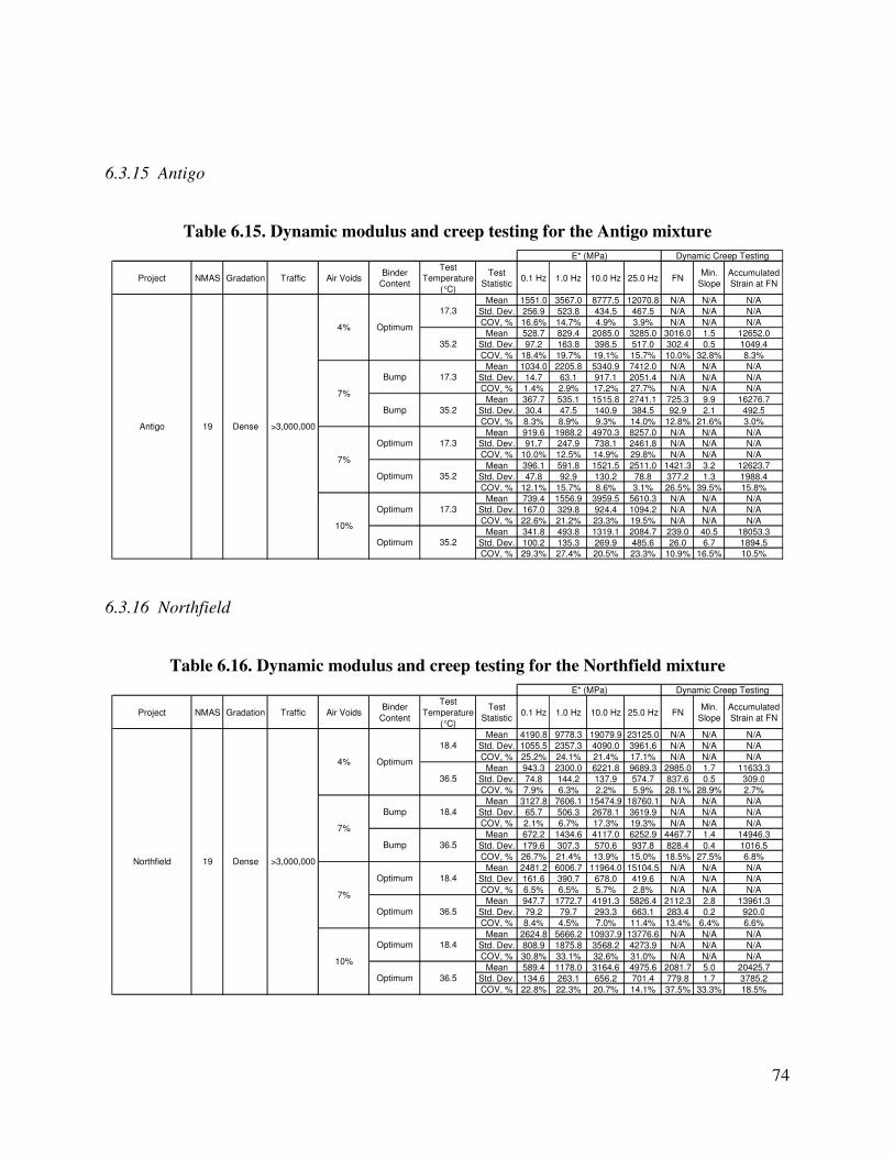
74
6.3.15 Antigo
Table 6.15. Dynamic modulus and creep testing for the Antigo mixture
Project NMAS Gradation Traffic Air VoidsBinder
Content
Test
Temperature
(°C)
Test
Statistic0.1 Hz 1.0 Hz 10.0 Hz 25.0 Hz FN
Min.
Slope
Accumulated
Strain at FN
Mean 1551.0 3567.0 8777.5 12070.8 N/A N/A N/A
Std. Dev. 256.9 523.8 434.5 467.5 N/A N/A N/A
COV, % 16.6% 14.7% 4.9% 3.9% N/A N/A N/A
Mean 528.7 829.4 2085.0 3285.0 3016.0 1.5 12652.0
Std. Dev. 97.2 163.8 398.5 517.0 302.4 0.5 1049.4
COV, % 18.4% 19.7% 19.1% 15.7% 10.0% 32.8% 8.3%
Mean 1034.0 2205.8 5340.9 7412.0 N/A N/A N/A
Std. Dev. 14.7 63.1 917.1 2051.4 N/A N/A N/A
COV, % 1.4% 2.9% 17.2% 27.7% N/A N/A N/A
Mean 367.7 535.1 1515.8 2741.1 725.3 9.9 16276.7
Std. Dev. 30.4 47.5 140.9 384.5 92.9 2.1 492.5
COV, % 8.3% 8.9% 9.3% 14.0% 12.8% 21.6% 3.0%
Mean 919.6 1988.2 4970.3 8257.0 N/A N/A N/A
Std. Dev. 91.7 247.9 738.1 2461.8 N/A N/A N/A
COV, % 10.0% 12.5% 14.9% 29.8% N/A N/A N/A
Mean 396.1 591.8 1521.5 2511.0 1421.3 3.2 12623.7
Std. Dev. 47.8 92.9 130.2 78.8 377.2 1.3 1988.4
COV, % 12.1% 15.7% 8.6% 3.1% 26.5% 39.5% 15.8%
Mean 739.4 1556.9 3959.5 5610.3 N/A N/A N/A
Std. Dev. 167.0 329.8 924.4 1094.2 N/A N/A N/A
COV, % 22.6% 21.2% 23.3% 19.5% N/A N/A N/A
Mean 341.8 493.8 1319.1 2084.7 239.0 40.5 18053.3
Std. Dev. 100.2 135.3 269.9 485.6 26.0 6.7 1894.5
COV, % 29.3% 27.4% 20.5% 23.3% 10.9% 16.5% 10.5%
E* (MPa) Dynamic Creep Testing
Antigo 19 Dense >3,000,000
4% Optimum
17.3
35.2
7%
Bump 17.3
Bump 35.2
7%
Optimum 17.3
Optimum 35.2
10%
Optimum 17.3
Optimum 35.2
6.3.16 Northfield
Table 6.16. Dynamic modulus and creep testing for the Northfield mixture
Project NMAS Gradation Traffic Air VoidsBinder
Content
Test
Temperature
(°C)
Test
Statistic0.1 Hz 1.0 Hz 10.0 Hz 25.0 Hz FN
Min.
Slope
Accumulated
Strain at FN
Mean 4190.8 9778.3 19079.9 23125.0 N/A N/A N/A
Std. Dev. 1055.5 2357.3 4090.0 3961.6 N/A N/A N/A
COV, % 25.2% 24.1% 21.4% 17.1% N/A N/A N/A
Mean 943.3 2300.0 6221.8 9689.3 2985.0 1.7 11633.3
Std. Dev. 74.8 144.2 137.9 574.7 837.6 0.5 309.0
COV, % 7.9% 6.3% 2.2% 5.9% 28.1% 28.9% 2.7%
Mean 3127.8 7606.1 15474.9 18760.1 N/A N/A N/A
Std. Dev. 65.7 506.3 2678.1 3619.9 N/A N/A N/A
COV, % 2.1% 6.7% 17.3% 19.3% N/A N/A N/A
Mean 672.2 1434.6 4117.0 6252.9 4467.7 1.4 14946.3
Std. Dev. 179.6 307.3 570.6 937.8 828.4 0.4 1016.5
COV, % 26.7% 21.4% 13.9% 15.0% 18.5% 27.5% 6.8%
Mean 2481.2 6006.7 11964.0 15104.5 N/A N/A N/A
Std. Dev. 161.6 390.7 678.0 419.6 N/A N/A N/A
COV, % 6.5% 6.5% 5.7% 2.8% N/A N/A N/A
Mean 947.7 1772.7 4191.3 5826.4 2112.3 2.8 13961.3
Std. Dev. 79.2 79.7 293.3 663.1 283.4 0.2 920.0
COV, % 8.4% 4.5% 7.0% 11.4% 13.4% 6.4% 6.6%
Mean 2624.8 5666.2 10937.9 13776.6 N/A N/A N/A
Std. Dev. 808.9 1875.8 3568.2 4273.9 N/A N/A N/A
COV, % 30.8% 33.1% 32.6% 31.0% N/A N/A N/A
Mean 589.4 1178.0 3164.6 4975.6 2081.7 5.0 20425.7
Std. Dev. 134.6 263.1 656.2 701.4 779.8 1.7 3785.2
COV, % 22.8% 22.3% 20.7% 14.1% 37.5% 33.3% 18.5%
10%
Optimum 18.4
Optimum 36.5
7%
Optimum 18.4
Optimum 36.5
7%
Bump 18.4
Bump 36.5
4% Optimum
18.4
36.5
Northfield 19 Dense >3,000,000
E* (MPa) Dynamic Creep Testing

75
6.3.17 Wisconsin Rapids
Table 6.17. Dynamic modulus and creep testing for the Wisconsin Rapids mixture
Project NMAS Gradation Traffic Air VoidsBinder
Content
Test
Temperature
(°C)
Test
Statistic0.1 Hz 1.0 Hz 10.0 Hz 25.0 Hz FN
Min.
Slope
Accumulated
Strain at FN
Mean 3857.6 9768.8 20501.9 26066.9 N/A N/A N/A
Std. Dev. 516.2 982.4 2802.6 3735.4 N/A N/A N/A
COV, % 13.4% 10.1% 13.7% 14.3% N/A N/A N/A
Mean 603.2 1240.6 5317.4 8942.5 2365.3 2.3 13094.3
Std. Dev. 157.9 437.7 2328.7 3113.3 1176.3 1.2 1431.0
COV, % 26.2% 35.3% 43.8% 34.8% 49.7% 52.5% 10.9%
Mean 3281.0 8090.4 16007.9 19866.1 N/A N/A N/A
Std. Dev. 420.2 1192.5 3002.7 3504.3 N/A N/A N/A
COV, % 12.8% 14.7% 18.8% 17.6% N/A N/A N/A
Mean 474.1 975.7 3378.0 5629.0 1076.0 10.2 21902.0
Std. Dev. 66.4 188.4 803.5 2115.8 335.6 4.3 4264.1
COV, % 14.0% 19.3% 23.8% 37.6% 31.2% 42.3% 19.5%
Mean 2586.9 7055.6 16404.3 20837.2 N/A N/A N/A
Std. Dev. 296.7 920.2 1980.5 2077.1 N/A N/A N/A
COV, % 11.5% 13.0% 12.1% 10.0% N/A N/A N/A
Mean 466.7 940.1 3267.4 4899.8 1024.7 9.0 17924.3
Std. Dev. 56.1 122.7 581.6 937.7 364.5 4.0 1140.9
COV, % 12.0% 13.1% 17.8% 19.1% 35.6% 44.5% 6.4%
Mean 2706.0 7106.7 15883.6 20204.5 N/A N/A N/A
Std. Dev. 963.4 2226.2 4442.1 5723.3 N/A N/A N/A
COV, % 35.6% 31.3% 28.0% 28.3% N/A N/A N/A
Mean 529.6 980.7 3504.2 6173.9 579.7 20.0 22173.3
Std. Dev. 173.8 206.6 461.8 1545.7 76.0 3.4 1246.3
COV, % 32.8% 21.1% 13.2% 25.0% 13.1% 17.0% 5.6%
10%
Optimum 19.0
Optimum 37.5
7%
Optimum 19.0
Optimum 37.5
7%
Bump 19.0
Bump 37.5
4% Optimum
19.0
37.5
Wisconsin Rapids 19 Open >3,000,000
E* (MPa) Dynamic Creep Testing
6.3.18 Antigo
Table 6.18. Dynamic modulus and creep testing for the Antigo mixture
Project NMAS Gradation Traffic Air VoidsBinder
Content
Test
Temperature
(°C)
Test
Statistic0.1 Hz 1.0 Hz 10.0 Hz 25.0 Hz FN
Min.
Slope
Accumulated
Strain at FN
Mean 1213.4 2627.3 6493.7 10282.7 N/A N/A N/A
Std. Dev. 108.0 155.2 953.7 2110.4 N/A N/A N/A
COV, % 8.9% 5.9% 14.7% 20.5% N/A N/A N/A
Mean 494.2 734.6 1875.5 2746.3 4704.0 0.8 11820.0
Std. Dev. 94.1 117.9 430.9 487.2 985.4 0.1 1981.8
COV, % 19.0% 16.1% 23.0% 17.7% 20.9% 8.6% 16.8%
Mean 808.9 1663.6 4011.7 6427.9 N/A N/A N/A
Std. Dev. 120.1 247.1 775.6 1370.7 N/A N/A N/A
COV, % 14.8% 14.9% 19.3% 21.3% N/A N/A N/A
Mean 428.6 582.4 1874.2 3115.8 516.3 14.6 14873.7
Std. Dev. 99.1 88.2 612.1 1062.6 230.6 2.6 6993.1
COV, % 23.1% 15.1% 32.7% 34.1% 44.7% 17.7% 47.0%
Mean 1047.1 2355.3 6589.8 9321.4 N/A N/A N/A
Std. Dev. 183.6 433.1 1236.7 2022.2 N/A N/A N/A
COV, % 17.5% 18.4% 18.8% 21.7% N/A N/A N/A
Mean 445.5 669.3 1793.9 2893.1 858.0 8.5 16472.3
Std. Dev. 55.3 81.5 301.4 473.2 103.0 1.7 664.6
COV, % 12.4% 12.2% 16.8% 16.4% 12.0% 20.5% 4.0%
Mean 602.5 1279.1 3109.1 4530.8 N/A N/A N/A
Std. Dev. 24.0 89.0 142.1 145.2 N/A N/A N/A
COV, % 4.0% 7.0% 4.6% 3.2% N/A N/A N/A
Mean 307.2 412.0 1154.9 1877.6 560.3 17.5 19189.0
Std. Dev. 54.0 132.1 161.5 162.2 184.3 1.0 2882.0
COV, % 17.6% 32.1% 14.0% 8.6% 32.9% 5.6% 15.0%
E* (MPa) Dynamic Creep Testing
4%
7%
7%
Antigo 12.5 Dense >3,000,000
10%
Optimum
17.3
35.2
17.3Bump
35.2
Optimum
Bump
Optimum
Optimum
Optimum
17.3
35.2
17.3
35.2

76
6.3.19 Plymouth
Table 6.19. Dynamic modulus and creep testing for the Plymouth mixture
Project NMAS Gradation Traffic Air VoidsBinder
Content
Test
Temperature
(°C)
Test
Statistic0.1 Hz 1.0 Hz 10.0 Hz 25.0 Hz FN
Min.
Slope
Accumulated
Strain at FN
Mean 3642.5 8619.1 19712.6 27204.8 N/A N/A N/A
Std. Dev. 625.3 1965.9 5685.8 5243.5 N/A N/A N/A
COV, % 17.2% 22.8% 28.8% 19.3% N/A N/A N/A
Mean 837.1 1514.8 4870.8 8095.9 2093.3 2.9 13899.3
Std. Dev. 168.9 170.5 384.4 1568.4 360.7 0.5 1233.5
COV, % 20.2% 11.3% 7.9% 19.4% 17.2% 17.5% 8.9%
Mean 2196.7 5469.7 13107.5 17813.5 N/A N/A N/A
Std. Dev. 144.0 331.7 1850.5 3133.9 N/A N/A N/A
COV, % 6.6% 6.1% 14.1% 17.6% N/A N/A N/A
Mean 636.7 1104.9 3462.4 5556.1 974.0 14.1 22967.3
Std. Dev. 51.3 104.9 279.3 420.3 482.4 8.2 5319.6
COV, % 8.1% 9.5% 8.1% 7.6% 49.5% 58.5% 23.2%
Mean 2860.0 6715.8 17406.4 21691.4 N/A N/A N/A
Std. Dev. 305.4 774.1 1137.7 1844.3 N/A N/A N/A
COV, % 10.7% 11.5% 6.5% 8.5% N/A N/A N/A
Mean 739.1 1323.4 4183.5 7106.8 960.0 8.0 15134.0
Std. Dev. 121.7 178.1 764.1 1881.4 208.8 1.5 2796.7
COV, % 16.5% 13.5% 18.3% 26.5% 21.8% 18.5% 18.5%
Mean 1881.7 4553.7 10832.1 14109.9 N/A N/A N/A
Std. Dev. 169.9 917.0 1686.1 1428.3 N/A N/A N/A
COV, % 9.0% 20.1% 15.6% 10.1% N/A N/A N/A
Mean 570.4 973.9 3235.7 4932.0 453.0 22.7 18900.0
Std. Dev. 85.4 81.8 396.6 680.5 45.6 0.6 1493.4
COV, % 15.0% 8.4% 12.3% 13.8% 10.1% 2.8% 7.9%
10%
Optimum 19.7
Optimum 37.3
7%
Optimum 19.7
Optimum 37.3
7%
Bump 19.7
Bump 37.3
4% Optimum
19.7
37.3
Plymouth 12.5 Dense >3,000,000
E* (MPa) Dynamic Creep Testing
6.3.20 Racine
Table 6.20 Dynamic modulus and creep testing for the Racine mixture
Project NMAS Gradation Traffic Air VoidsBinder
Content
Test
Temperature
(°C)
Test
Statistic0.1 Hz 1.0 Hz 10.0 Hz 25.0 Hz FN
Min.
Slope
Accumulated
Strain at FN
Mean 1653.8 3382.8 8809.8 12551.2 N/A N/A N/A
Std. Dev. 306.3 525.6 2107.3 3382.9 N/A N/A N/A
COV, % 18.5% 15.5% 23.9% 27.0% N/A N/A N/A
Mean 749.7 1114.9 3150.9 4936.7 5290.7 0.9 12421.7
Std. Dev. 43.6 84.7 277.9 730.6 1501.3 0.0 3031.0
COV, % 5.8% 7.6% 8.8% 14.8% 28.4% 4.9% 24.4%
Mean 1191.0 2408.0 6078.8 8294.0 N/A N/A N/A
Std. Dev. 192.1 475.6 705.6 1144.1 N/A N/A N/A
COV, % 16.1% 19.8% 11.6% 13.8% N/A N/A N/A
Mean 559.3 765.6 2002.2 3133.8 1228.0 8.5 20440.3
Std. Dev. 52.4 51.5 60.4 83.8 490.4 5.1 2907.8
COV, % 9.4% 6.7% 3.0% 2.7% 39.9% 60.2% 14.2%
Mean 1423.2 2864.3 6662.9 9247.5 N/A N/A N/A
Std. Dev. 117.9 272.3 631.5 198.7 N/A N/A N/A
COV, % 8.3% 9.5% 9.5% 2.1% N/A N/A N/A
Mean 651.6 963.8 2689.3 4333.5 1624.0 4.5 16204.3
Std. Dev. 21.0 92.2 413.8 675.8 485.6 1.0 2834.6
COV, % 3.2% 9.6% 15.4% 15.6% 29.9% 22.3% 17.5%
Mean 855.6 1838.9 4306.2 5600.8 N/A N/A N/A
Std. Dev. 24.6 52.8 105.1 261.5 N/A N/A N/A
COV, % 2.9% 2.9% 2.4% 4.7% N/A N/A N/A
Mean 403.5 559.1 1437.9 2187.3 715.3 16.0 22166.7
Std. Dev. 34.2 37.5 58.3 104.6 94.6 1.5 1622.6
COV, % 8.5% 6.7% 4.1% 4.8% 13.2% 9.5% 7.3%
10%
Optimum 20.9
Optimum 39.2
7%
Optimum 20.9
Optimum 39.2
7%
Bump 20.9
Bump 39.2
4% Optimum
20.9
39.2
Racine 12.5 Dense >3,000,000
E* (MPa) Dynamic Creep Testing

77
6.3.21 Northfield
Table 6.21. Dynamic modulus and creep testing for the Northfield mixture
Project NMAS Gradation Traffic Air VoidsBinder
Content
Test
Temperature
(°C)
Test
Statistic0.1 Hz 1.0 Hz 10.0 Hz 25.0 Hz FN
Min.
Slope
Accumulated
Strain at FN
Mean 868.1 1834.1 4437.2 6974.8 N/A N/A N/A
Std. Dev. 116.4 338.3 1104.6 1283.3 N/A N/A N/A
COV, % 13.4% 18.4% 24.9% 18.4% N/A N/A N/A
Mean 385.1 536.5 1425.5 3192.3 2622.7 2.5 17659.7
Std. Dev. 47.3 61.1 160.5 792.6 888.8 0.5 1367.1
COV, % 12.3% 11.4% 11.3% 24.8% 33.9% 21.0% 7.7%
Mean 1094.6 2187.2 6478.2 13989.4 N/A N/A N/A
Std. Dev. 147.4 314.7 2207.0 3059.4 N/A N/A N/A
COV, % 13.5% 14.4% 34.1% 21.9% N/A N/A N/A
Mean 448.9 631.8 2528.9 3990.4 4986.7 1.4 20109.0
Std. Dev. 20.5 50.2 1613.0 1914.4 1146.7 0.1 1871.8
COV, % 4.6% 7.9% 63.8% 48.0% 23.0% 9.7% 9.3%
Mean 886.3 1775.4 4146.2 7466.9 N/A N/A N/A
Std. Dev. 124.6 189.9 548.7 628.0 N/A N/A N/A
COV, % 14.1% 10.7% 13.2% 8.4% N/A N/A N/A
Mean 484.6 703.4 1970.1 3560.5 5840.0 1.1 17121.7
Std. Dev. 43.0 65.7 131.9 935.3 1304.1 0.4 772.1
COV, % 8.9% 9.3% 6.7% 26.3% 22.3% 34.0% 4.5%
Mean 1156.3 2314.4 6125.3 9013.3 N/A N/A N/A
Std. Dev. 26.4 216.4 1152.2 2082.1 N/A N/A N/A
COV, % 2.3% 9.4% 18.8% 23.1% N/A N/A N/A
Mean 393.2 558.2 1627.8 2897.6 6104.0 1.0 17942.3
Std. Dev. 18.9 51.0 236.4 503.1 1845.9 0.2 1946.2
COV, % 4.8% 9.1% 14.5% 17.4% 30.2% 21.8% 10.8%
10%
Optimum 18.4
Optimum 36.5
7%
Optimum 18.4
Optimum 36.5
7%
Bump 18.4
Bump 36.5
4% Optimum
18.4
36.5
Northfield 12.5 Open >3,000,000
E* (MPa) Dynamic Creep Testing
6.3.22 Pooled Data for Database
Table 6.22. Pooled dynamic modulus and creep testing for dense-graded mixture with an
NMAS of 19.0 mm and 300,000 ESAL traffic level
NMAS Gradation TrafficAir Voids,
%
Binder
Content
Mean Test
Temperature, °C
Test
Statistic0.1 Hz 1.0 Hz 10.0 Hz 25.0 Hz FN Min. Slope
Accumulated
Strain at FNMean 1711.9 4513.5 11374.3 18456.8 N/A N/A N/A
Std. Dev. 321.1 872.5 1470.0 2794.6 N/A N/A N/A
COV, % 18.8% 19.3% 12.9% 15.1% N/A N/A N/A
Mean 474.8 800.0 2381.5 3849.8 140.7 45.3 10913.0
Std. Dev. 10.2 54.4 174.9 492.4 18.9 4.1 947.6
COV, % 2.1% 6.8% 7.3% 12.8% 13.5% 8.9% 8.7%
Mean 1330.3 3762.8 10394.8 18857.1 N/A N/A N/A
Std. Dev. 71.6 474.5 461.9 2398.7 N/A N/A N/A
COV, % 5.4% 12.6% 4.4% 12.7% N/A N/A N/A
Mean 426.4 697.3 1998.9 2991.9 74.0 165.4 16647.3
Std. Dev. 64.7 87.1 161.9 347.4 10.0 17.1 1172.5
COV, % 15.2% 12.5% 8.1% 11.6% 13.5% 10.3% 7.0%
Mean 1438.1 3768.3 8756.4 15191.1 N/A N/A N/A
Std. Dev. 83.8 639.3 1292.3 3973.6 N/A N/A N/A
COV, % 5.8% 17.0% 14.8% 26.2% N/A N/A N/A
Mean 383.4 617.7 1984.1 3090.8 75.7 135.8 14743.7
Std. Dev. 68.0 86.7 185.2 682.0 10.4 12.9 592.0
COV, % 17.7% 14.0% 9.3% 22.1% 13.8% 9.5% 4.0%
Mean 1114.0 2878.4 7305.7 15268.7 N/A N/A N/A
Std. Dev. 191.4 654.7 1454.2 1990.2 N/A N/A N/A
COV, % 17.2% 22.7% 19.9% 13.0% N/A N/A N/A
Mean 290.7 476.2 1370.2 2287.6 37.3 398.2 18501.0
Std. Dev. 31.7 47.2 114.7 322.5 2.9 53.1 727.5
COV, % 10.9% 9.9% 8.4% 14.1% 7.7% 13.3% 3.9%
35.5
35.5
16.6
35.5
16.6
19 Dense 300,000
4
7
7
10
Optimum
Pooled Dynamic Creep Test DataPooled E* by Frequency (MPa)
Bump
Optimum
Optimum
16.6
35.5
16.6

78
Table 6.23. Pooled dynamic modulus and creep testing for dense-graded mixture with an
NMAS of 12.5 mm and 300,000 ESAL traffic level
NMAS Gradation TrafficAir Voids,
%
Binder
Content
Mean Test
Temperature, °C
Test
Statistic0.1 Hz 1.0 Hz 10.0 Hz 25.0 Hz FN Min. Slope
Accumulated
Strain at FNMean 1649.3 3954.0 8895.4 13431.1 N/A N/A N/A
Std. Dev. 270.1 665.7 1405.1 1558.1 N/A N/A N/A
COV, % 16.4% 16.8% 15.8% 11.6% N/A N/A N/A
Mean 415.8 735.8 2432.0 4164.6 179.8 54.2 14878.5
Std. Dev. 39.7 55.0 236.5 486.5 23.1 4.8 1333.8
COV, % 9.6% 7.5% 9.7% 11.7% 12.8% 8.9% 9.0%
Mean 997.4 2476.0 5923.6 8507.6 N/A N/A N/A
Std. Dev. 68.4 94.5 383.7 393.7 N/A N/A N/A
COV, % 6.9% 3.8% 6.5% 4.6% N/A N/A N/A
Mean 265.0 477.2 1465.3 2442.3 98.2 167.7 22018.7
Std. Dev. 28.4 58.7 153.8 405.8 21.4 33.6 1262.7
COV, % 10.7% 12.3% 10.5% 16.6% 21.8% 20.0% 5.7%
Mean 1351.3 3341.2 7766.4 11902.8 N/A N/A N/A
Std. Dev. 131.2 341.7 1024.2 1408.6 N/A N/A N/A
COV, % 9.7% 10.2% 13.2% 11.8% N/A N/A N/A
Mean 338.0 617.4 2163.0 3373.5 90.7 140.8 17588.5
Std. Dev. 18.6 50.5 268.2 710.9 14.3 25.0 1310.0
COV, % 5.5% 8.2% 12.4% 21.1% 15.7% 17.8% 7.4%
Mean 940.7 2312.3 5675.3 8730.8 N/A N/A N/A
Std. Dev. 57.8 63.8 488.2 1557.7 N/A N/A N/A
COV, % 6.1% 2.8% 8.6% 17.8% N/A N/A N/A
Mean 259.8 440.9 1355.5 2552.1 54.0 332.3 22963.8
Std. Dev. 50.9 73.3 173.7 388.6 2.9 50.0 2304.6
COV, % 19.6% 16.6% 12.8% 15.2% 5.3% 15.0% 10.0%
10 Optimum
17.8
36.2
Bump
17.8
36.2
7 Optimum
17.8
36.2
Pooled E* (MPa)
12.5 Dense 300,000
4 Optimum
17.8
36.2
7
Pooled Dynamic Creep Test Data
Table 6.24. Pooled dynamic modulus and creep testing for dense-graded mixture with an
NMAS of 19.0 mm and 1,000,000 ESAL traffic level
NMAS Gradation TrafficAir Voids,
%
Binder
Content
Mean Test
Temperature, °C
Test
Statistic0.1 Hz 1.0 Hz 10.0 Hz 25.0 Hz FN Min. Slope
Accumulated
Strain at FN
Mean 2106.3 5038.8 11046.2 16028.9 N/A N/A N/A
Std. Dev. 176.9 681.2 1922.6 2674.2 N/A N/A N/A
COV, % 8.4% 13.5% 17.4% 16.7% N/A N/A N/A
Mean 662.9 1159.1 2991.7 4854.5 607.3 14.7 13111.8
Std. Dev. 94.8 150.9 182.9 406.4 100.4 2.7 1137.0
COV, % 14.3% 13.0% 6.1% 8.4% 16.5% 18.5% 8.7%
Mean 1365.2 3171.7 7622.7 11143.4 N/A N/A N/A
Std. Dev. 199.8 484.0 1963.8 2690.5 N/A N/A N/A
COV, % 14.6% 15.3% 25.8% 24.1% N/A N/A N/A
Mean 458.7 758.7 1920.1 3190.1 149.0 77.6 17497.2
Std. Dev. 76.2 127.5 214.8 320.6 21.4 3.0 1483.9
COV, % 16.6% 16.8% 11.2% 10.1% 14.4% 3.9% 8.5%
Mean 1390.3 3243.6 7263.6 10674.6 N/A N/A N/A
Std. Dev. 187.0 664.7 1769.9 3461.1 N/A N/A N/A
COV, % 13.4% 20.5% 24.4% 32.4% N/A N/A N/A
Mean 495.9 854.8 2413.6 3713.1 135.7 76.1 16381.7
Std. Dev. 73.5 120.2 423.7 495.8 19.0 6.9 1053.8
COV, % 14.8% 14.1% 17.6% 13.4% 14.0% 9.1% 6.4%
Mean 914.2 2062.3 4990.2 7758.0 N/A N/A N/A
Std. Dev. 64.3 107.4 138.7 897.9 N/A N/A N/A
COV, % 7.0% 5.2% 2.8% 11.6% N/A N/A N/A
Mean 535.1 965.4 1871.0 2808.5 70.7 174.7 17711.0
Std. Dev. 190.0 297.1 228.6 273.5 13.2 19.8 1212.5
COV, % 35.5% 30.8% 12.2% 9.7% 18.7% 11.4% 6.8%
Optimum
18.7
37.2
10 Optimum
18.7
37.2
Optimum
18.7
37.2
7 Bump
18.7
37.2
19 Dense 1,000,000
4
7
Pooled E* (MPa) Pooled Dynamic Creep Test Data

79
Table 6.25. Pooled dynamic modulus and creep testing for dense-graded mixture with an
NMAS of 12.5 mm and 1,000,000 ESAL traffic level
NMAS Gradation TrafficAir Voids,
%
Binder
Content
Mean Test
Temperature, °C
Test
Statistic0.1 Hz 1.0 Hz 10.0 Hz 25.0 Hz FN Min. Slope
Accumulated
Strain at FNMean 1889.8 4680.4 10470.6 14176.7 N/A N/A N/A
Std. Dev. 182.2 450.4 1466.6 1186.9 N/A N/A N/A
COV, % 9.6% 9.6% 14.0% 8.4% N/A N/A N/A
Mean 515.6 978.0 3453.7 5229.1 260.2 32.5 13702.8
Std. Dev. 16.6 76.9 351.7 838.5 44.7 5.6 2996.3
COV, % 3.2% 7.9% 10.2% 16.0% 17.2% 17.3% 21.9%
Mean 1346.9 3505.4 8052.4 10654.7 N/A N/A N/A
Std. Dev. 206.1 744.1 1972.1 2750.4 N/A N/A N/A
COV, % 15.3% 21.2% 24.5% 25.8% N/A N/A N/A
Mean 346.5 624.1 2293.4 3303.6 124.8 107.9 18582.0
Std. Dev. 68.4 123.8 418.5 639.1 24.0 9.6 2569.8
COV, % 19.7% 19.8% 18.2% 19.3% 19.3% 8.9% 13.8%
Mean 1172.4 2928.1 6952.2 11576.5 N/A N/A N/A
Std. Dev. 130.9 345.5 712.7 1467.2 N/A N/A N/A
COV, % 11.2% 11.8% 10.3% 12.7% N/A N/A N/A
Mean 387.2 727.8 2496.7 3719.2 121.5 99.5 16509.2
Std. Dev. 73.6 181.8 512.6 578.5 11.5 12.8 1571.0
COV, % 19.0% 25.0% 20.5% 15.6% 9.5% 12.8% 9.5%
Mean 1017.2 2471.8 6245.4 8835.0 N/A N/A N/A
Std. Dev. 123.7 258.1 682.3 1310.2 N/A N/A N/A
COV, % 12.2% 10.4% 10.9% 14.8% N/A N/A N/A
Mean 268.9 467.4 1552.4 2336.5 67.3 291.9 23756.7
Std. Dev. 32.5 63.7 191.5 353.4 1.4 18.2 704.3
COV, % 12.1% 13.6% 12.3% 15.1% 2.1% 6.2% 3.0%
Optimum
18.2
36.7
10 Optimum
18.2
36.7
Optimum
18.2
36.7
7 Bump
18.2
36.7
12.5 Dense 1,000,000
4
7
Pooled E* (MPa) Pooled Dynamic Creep Test Data
Table 6.26. Pooled dynamic modulus and creep testing for open-graded mixture with an
NMAS of 25.0 mm and 3,000,000 ESAL traffic level
NMAS Gradation TrafficAir Voids,
%
Binder
Content
Mean Test
Temperature, °C
Test
Statistic0.1 Hz 1.0 Hz 10.0 Hz 25.0 Hz FN Min. Slope
Accumulated
Strain at FNMean 3964.5 10368.2 27417.1 34924.2 N/A N/A N/A
Std. Dev. 635.7 548.5 3327.4 4848.2 N/A N/A N/A
COV, % 16.0% 5.3% 12.1% 13.9% N/A N/A N/A
Mean 938.4 1674.3 5297.5 9301.6 2880.0 2.5 16225.3
Std. Dev. 72.5 266.3 829.9 730.0 524.4 0.5 1020.6
COV, % 7.7% 15.9% 15.7% 7.8% 18.2% 22.1% 6.3%
Mean 2070.7 5258.3 12004.0 14751.1 N/A N/A N/A
Std. Dev. 230.5 343.6 859.6 1238.2 N/A N/A N/A
COV, % 11.1% 6.5% 7.2% 8.4% N/A N/A N/A
Mean 471.6 870.6 3320.1 5541.7 774.0 20.1 26157.0
Std. Dev. 85.2 148.7 704.7 1011.3 101.1 2.6 4543.5
COV, % 18.1% 17.1% 21.2% 18.2% 13.1% 13.1% 17.4%
Mean 2913.2 6942.3 15695.8 20416.9 N/A N/A N/A
Std. Dev. 622.6 875.5 744.0 1249.8 N/A N/A N/A
COV, % 21.4% 12.6% 4.7% 6.1% N/A N/A N/A
Mean 562.8 1032.4 4118.9 6826.6 1387.3 7.1 20829.3
Std. Dev. 111.9 177.4 1259.2 1893.5 615.5 3.5 6672.6
COV, % 19.9% 17.2% 30.6% 27.7% 44.4% 49.5% 32.0%
Mean 2158.8 5286.9 13680.9 17857.8 N/A N/A N/A
Std. Dev. 187.2 500.7 1920.7 2226.2 N/A N/A N/A
COV, % 8.7% 9.5% 14.0% 12.5% N/A N/A N/A
Mean 509.6 862.9 2999.7 4825.7 447.7 29.7 21742.7
Std. Dev. 38.3 34.2 170.4 987.1 47.5 1.9 676.1
COV, % 7.5% 4.0% 5.7% 20.5% 10.6% 6.3% 3.1%
Optimum
17.3
35.6
10 Optimum
17.3
35.6
Optimum
17.3
35.6
7 Bump
17.3
35.6
25 Open 3,000,000
4
7
Pooled E* (MPa) Pooled Dynamic Creep Test Data

80
Table 6.27. Pooled dynamic modulus and creep testing for dense-graded mixture with an
NMAS of 19.0 mm and 3,000,000 ESAL traffic level
NMAS Gradation TrafficAir Voids,
%
Binder
Content
Mean Test
Temperature, °C
Test
Statistic0.1 Hz 1.0 Hz 10.0 Hz 25.0 Hz FN Min. Slope
Accumulated
Strain at FNMean 1781.6 4306.5 10278.9 15907.1 N/A N/A N/A
Std. Dev. 183.4 701.4 2178.5 3660.4 N/A N/A N/A
COV, % 10.3% 16.3% 21.2% 23.0% N/A N/A N/A
Mean 501.9 926.8 3059.1 5616.5 532.2 24.0 12415.9
Std. Dev. 63.3 123.2 446.0 915.6 133.7 2.8 1364.3
COV, % 12.6% 13.3% 14.6% 16.3% 25.1% 11.8% 11.0%
Mean 1237.7 2958.2 6917.8 10048.0 N/A N/A N/A
Std. Dev. 156.0 308.9 829.7 1417.9 N/A N/A N/A
COV, % 12.6% 10.4% 12.0% 14.1% N/A N/A N/A
Mean 417.0 722.5 2145.1 3525.6 215.1 80.6 17055.7
Std. Dev. 68.8 111.7 427.3 865.8 19.6 7.9 1221.4
COV, % 16.5% 15.5% 19.9% 24.6% 9.1% 9.8% 7.2%
Mean 1465.1 3515.8 8304.6 12138.4 N/A N/A N/A
Std. Dev. 197.4 499.7 1024.3 1306.4 N/A N/A N/A
COV, % 13.5% 14.2% 12.3% 10.8% N/A N/A N/A
Mean 430.0 762.5 2524.2 4489.5 206.8 78.6 15360.7
Std. Dev. 64.6 83.6 243.1 597.3 41.4 2.3 1680.0
COV, % 15.0% 11.0% 9.6% 13.3% 20.0% 2.9% 10.9%
Mean 1077.2 2638.2 6472.8 9697.7 N/A N/A N/A
Std. Dev. 106.4 386.6 1336.9 1743.9 N/A N/A N/A
COV, % 9.9% 14.7% 20.7% 18.0% N/A N/A N/A
Mean 346.6 590.4 1875.1 3041.8 86.8 211.9 19014.9
Std. Dev. 68.5 97.4 586.3 787.6 7.5 16.4 1335.1
COV, % 19.8% 16.5% 31.3% 25.9% 8.7% 7.7% 7.0%
Optimum
18.8
36.9
10 Optimum
18.8
36.9
Optimum
18.8
36.9
7 Bump
18.8
36.9
19 Dense 3,000,000
4
7
Pooled E* (MPa) Pooled Dynamic Creep Test Data
Table 6.28. Pooled dynamic modulus and creep testing for dense-graded mixture with an
NMAS of 12.5 mm and 3,000,000 ESAL traffic level
NMAS Gradation TrafficAir Voids,
%
Binder
Content
Mean Test
Temperature, °C
Test
Statistic0.1 Hz 1.0 Hz 10.0 Hz 25.0 Hz FN Min. Slope
Accumulated
Strain at FNMean 2339.0 5179.9 11317.9 14398.1 N/A N/A N/A
Std. Dev. 255.9 419.1 1301.4 2158.5 N/A N/A N/A
COV, % 10.9% 8.1% 11.5% 15.0% N/A N/A N/A
Mean 618.1 1188.4 4026.1 5793.1 2649.3 37.3 12574.7
Std. Dev. 143.8 211.9 828.3 997.5 528.4 11.3 1464.3
COV, % 23.3% 17.8% 20.6% 17.2% 19.9% 30.2% 11.6%
Mean 1740.1 4068.3 8660.5 11045.1 N/A N/A N/A
Std. Dev. 260.5 548.9 632.0 877.6 N/A N/A N/A
COV, % 15.0% 13.5% 7.3% 7.9% N/A N/A N/A
Mean 465.0 874.7 2721.6 4564.2 563.8 148.2 19722.0
Std. Dev. 78.3 147.3 703.1 1435.8 313.5 69.0 3352.5
COV, % 16.8% 16.8% 25.8% 31.5% 55.6% 46.5% 17.0%
Mean 1646.0 3908.8 8713.8 12282.7 N/A N/A N/A
Std. Dev. 249.0 568.8 1111.2 2418.3 N/A N/A N/A
COV, % 15.1% 14.6% 12.8% 19.7% N/A N/A N/A
Mean 457.7 879.0 3068.0 4560.5 358.9 118.8 17147.2
Std. Dev. 144.4 215.1 552.0 998.4 91.9 30.4 1493.2
COV, % 31.6% 24.5% 18.0% 21.9% 25.6% 25.6% 8.7%
Mean 1187.4 2923.9 7444.0 10110.1 N/A N/A N/A
Std. Dev. 117.3 278.2 567.5 1303.6 N/A N/A N/A
COV, % 9.9% 9.5% 7.6% 12.9% N/A N/A N/A
Mean 327.6 597.6 1904.3 3155.3 200.3 234.6 25676.3
Std. Dev. 64.1 121.3 309.1 524.3 56.1 73.5 8920.6
COV, % 19.6% 20.3% 16.2% 16.6% 28.0% 31.3% 34.7%
Optimum
17.5
36.2
10 Optimum
17.5
36.2
Optimum
17.5
36.2
7 Bump
17.5
36.2
12.5 Dense 3,000,000
4
7
Pooled E* (MPa) Pooled Dynamic Creep Test Data

81
Table 6.29. Pooled dynamic modulus and creep testing for dense-graded mixture with an
NMAS of 19.0 mm and >3,000,000 ESAL traffic level
NMAS Gradation TrafficAir Voids,
%
Binder
Content
Mean Test
Temperature, °C
Test
Statistic0.1 Hz 1.0 Hz 10.0 Hz 25.0 Hz FN Min. Slope
Accumulated
Strain at FNMean 2870.9 6672.6 13928.7 17597.9 N/A N/A N/A
Std. Dev. 656.2 1440.6 2262.2 2214.6 N/A N/A N/A
COV, % 22.9% 21.6% 16.2% 12.6% N/A N/A N/A
Mean 736.0 1564.7 4153.4 6487.2 3000.5 1.6 12142.7
Std. Dev. 86.0 154.0 268.2 545.8 570.0 0.5 679.2
COV, % 11.7% 9.8% 6.5% 8.4% 19.0% 30.7% 5.6%
Mean 2080.9 4905.9 10407.9 13086.0 N/A N/A N/A
Std. Dev. 40.2 284.7 1797.6 2835.7 N/A N/A N/A
COV, % 1.9% 5.8% 17.3% 21.7% N/A N/A N/A
Mean 520.0 984.9 2816.4 4497.0 2596.5 5.6 15611.5
Std. Dev. 105.0 177.4 355.8 661.1 460.6 1.3 754.5
COV, % 20.2% 18.0% 12.6% 14.7% 17.7% 22.3% 4.8%
Mean 1700.4 3997.5 8467.2 11680.8 N/A N/A N/A
Std. Dev. 126.6 319.3 708.0 1440.7 N/A N/A N/A
COV, % 7.4% 8.0% 8.4% 12.3% N/A N/A N/A
Mean 671.9 1182.2 2856.4 4168.7 1766.8 3.0 13292.5
Std. Dev. 63.5 86.3 211.8 370.9 330.3 0.7 1454.2
COV, % 9.4% 7.3% 7.4% 8.9% 18.7% 24.0% 10.9%
Mean 1682.1 3611.5 7448.7 9693.5 N/A N/A N/A
Std. Dev. 487.9 1102.8 2246.3 2684.0 N/A N/A N/A
COV, % 29.0% 30.5% 30.2% 27.7% N/A N/A N/A
Mean 465.6 835.9 2241.9 3530.2 1160.3 22.7 19239.5
Std. Dev. 117.4 199.2 463.0 593.5 402.9 4.2 2839.9
COV, % 25.2% 23.8% 20.7% 16.8% 34.7% 18.3% 14.8%
Optimum
17.9
35.9
10 Optimum
17.9
35.9
Optimum
17.9
35.9
7 Bump
17.9
35.9
19 Dense >3,000,000
4
7
Pooled E* (MPa) Pooled Dynamic Creep Test Data
Table 6.30. Pooled dynamic modulus and creep testing for open-graded mixture with an
NMAS of 19.0 mm and >3,000,000 ESAL traffic level
NMAS Gradation TrafficAir Voids,
%
Binder
Content
Mean Test
Temperature, °C
Test
Statistic0.1 Hz 1.0 Hz 10.0 Hz 25.0 Hz FN Min. Slope
Accumulated
Strain at FNMean 3857.6 9768.8 20501.9 26066.9 N/A N/A N/A
Std. Dev. 516.2 982.4 2802.6 3735.4 N/A N/A N/A
COV, % 13.4% 10.1% 13.7% 14.3% N/A N/A N/A
Mean 603.2 1240.6 5317.4 8942.5 2365.3 2.3 13094.3
Std. Dev. 157.9 437.7 2328.7 3113.3 1176.3 1.2 1431.0
COV, % 26.2% 35.3% 43.8% 34.8% 49.7% 52.5% 10.9%
Mean 3281.0 8090.4 16007.9 19866.1 N/A N/A N/A
Std. Dev. 420.2 1192.5 3002.7 3504.3 N/A N/A N/A
COV, % 12.8% 14.7% 18.8% 17.6% N/A N/A N/A
Mean 474.1 975.7 3378.0 5629.0 1076.0 10.2 21902.0
Std. Dev. 66.4 188.4 803.5 2115.8 335.6 4.3 4264.1
COV, % 14.0% 19.3% 23.8% 37.6% 31.2% 42.3% 19.5%
Mean 2586.9 7055.6 16404.3 20837.2 N/A N/A N/A
Std. Dev. 296.7 920.2 1980.5 2077.1 N/A N/A N/A
COV, % 11.5% 13.0% 12.1% 10.0% N/A N/A N/A
Mean 466.7 940.1 3267.4 4899.8 1024.7 9.0 17924.3
Std. Dev. 56.1 122.7 581.6 937.7 364.5 4.0 1140.9
COV, % 12.0% 13.1% 17.8% 19.1% 35.6% 44.5% 6.4%
Mean 2706.0 7106.7 15883.6 20204.5 N/A N/A N/A
Std. Dev. 963.4 2226.2 4442.1 5723.3 N/A N/A N/A
COV, % 35.6% 31.3% 28.0% 28.3% N/A N/A N/A
Mean 529.6 980.7 3504.2 6173.9 579.7 20.0 22173.3
Std. Dev. 173.8 206.6 461.8 1545.7 76.0 3.4 1246.3
COV, % 32.8% 21.1% 13.2% 25.0% 13.1% 17.0% 5.6%
Optimum
19.0
37.5
10 Optimum
19.0
37.5
Optimum
19.0
37.5
7 Bump
19.0
37.5
19 Open >3,000,000
4
7
Pooled E* (MPa) Pooled Dynamic Creep Test Data

82
Table 6.31. Pooled dynamic modulus and creep testing for dense-graded mixture with an
NMAS of 12.5 mm and >3,000,000 ESAL traffic level
NMAS Gradation TrafficAir Voids,
%
Binder
Content
Mean Test
Temperature, °C
Test
Statistic0.1 Hz 1.0 Hz 10.0 Hz 25.0 Hz FN Min. Slope
Accumulated
Strain at FNMean 2169.9 4876.4 11672.0 16679.5 N/A N/A N/A
Std. Dev. 346.5 882.2 2915.6 3578.9 N/A N/A N/A
COV, % 16.0% 18.1% 25.0% 21.5% N/A N/A N/A
Mean 693.7 1121.4 3299.1 5259.7 4029.3 1.5 12713.7
Std. Dev. 102.2 124.4 364.4 928.7 949.1 0.2 2082.1
COV, % 14.7% 11.1% 11.0% 17.7% 23.6% 13.5% 16.4%
Mean 1398.9 3180.4 7732.7 10845.1 N/A N/A N/A
Std. Dev. 152.1 351.5 1110.6 1882.9 N/A N/A N/A
COV, % 10.9% 11.1% 14.4% 17.4% N/A N/A N/A
Mean 541.5 817.6 2446.2 3935.2 906.1 12.4 19427.1
Std. Dev. 67.6 81.5 317.3 522.3 401.1 5.3 5073.5
COV, % 12.5% 10.0% 13.0% 13.3% 44.3% 42.9% 26.1%
Mean 1776.8 3978.5 10219.7 13420.1 N/A N/A N/A
Std. Dev. 202.3 493.2 1002.0 1355.1 N/A N/A N/A
COV, % 11.4% 12.4% 9.8% 10.1% N/A N/A N/A
Mean 612.1 985.5 2888.9 4777.8 1147.3 7.0 15936.9
Std. Dev. 66.0 117.3 493.1 1010.1 265.8 1.4 2098.6
COV, % 10.8% 11.9% 17.1% 21.1% 23.2% 20.1% 13.2%
Mean 1113.2 2557.2 6082.5 8080.5 N/A N/A N/A
Std. Dev. 72.8 352.9 644.5 611.7 N/A N/A N/A
COV, % 6.5% 13.8% 10.6% 7.6% N/A N/A N/A
Mean 427.0 648.3 1942.9 2999.0 576.2 18.7 20085.2
Std. Dev. 57.9 83.8 205.5 315.7 108.2 1.0 1999.3
COV, % 13.5% 12.9% 10.6% 10.5% 18.8% 5.6% 10.0%
Optimum
19.3
37.2
10 Optimum
19.3
37.2
Optimum
19.3
37.2
7 Bump
19.3
37.2
12.5 Dense >3,000,000
4
7
Pooled E* (MPa) Pooled Dynamic Creep Test Data
Table 6.32. Pooled dynamic modulus and creep testing for open-graded mixture with an
NMAS of 12.5 mm and >3,000,000 ESAL traffic level
NMAS Gradation TrafficAir Voids,
%
Binder
Content
Mean Test
Temperature, °C
Test
Statistic0.1 Hz 1.0 Hz 10.0 Hz 25.0 Hz FN Min. Slope
Accumulated
Strain at FNMean 868.1 1834.1 4437.2 6974.8 N/A N/A N/A
Std. Dev. 116.4 338.3 1104.6 1283.3 N/A N/A N/A
COV, % 13.4% 18.4% 24.9% 18.4% N/A N/A N/A
Mean 385.1 536.5 1425.5 3192.3 2622.7 2.5 17659.7
Std. Dev. 47.3 61.1 160.5 792.6 888.8 0.5 1367.1
COV, % 12.3% 11.4% 11.3% 24.8% 33.9% 21.0% 7.7%
Mean 1094.6 2187.2 6478.2 13989.4 N/A N/A N/A
Std. Dev. 147.4 314.7 2207.0 3059.4 N/A N/A N/A
COV, % 13.5% 14.4% 34.1% 21.9% N/A N/A N/A
Mean 448.9 631.8 2528.9 3990.4 4986.7 1.4 20109.0
Std. Dev. 20.5 50.2 1613.0 1914.4 1146.7 0.1 1871.8
COV, % 4.6% 7.9% 63.8% 48.0% 23.0% 9.7% 9.3%
Mean 886.3 1775.4 4146.2 7466.9 N/A N/A N/A
Std. Dev. 124.6 189.9 548.7 628.0 N/A N/A N/A
COV, % 14.1% 10.7% 13.2% 8.4% N/A N/A N/A
Mean 484.6 703.4 1970.1 3560.5 5840.0 1.1 17121.7
Std. Dev. 43.0 65.7 131.9 935.3 1304.1 0.4 772.1
COV, % 8.9% 9.3% 6.7% 26.3% 22.3% 34.0% 4.5%
Mean 1156.3 2314.4 6125.3 9013.3 N/A N/A N/A
Std. Dev. 26.4 216.4 1152.2 2082.1 N/A N/A N/A
COV, % 2.3% 9.4% 18.8% 23.1% N/A N/A N/A
Mean 393.2 558.2 1627.8 2897.6 6104.0 1.0 17942.3
Std. Dev. 18.9 51.0 236.4 503.1 1845.9 0.2 1946.2
COV, % 4.8% 9.1% 14.5% 17.4% 30.2% 21.8% 10.8%
Optimum
18.4
36.5
10 Optimum
18.4
36.5
Optimum
18.4
36.5
7 Bump
18.4
36.5
12.5 Open >3,000,000
4
7
Pooled E* (MPa) Pooled Dynamic Creep Test Data

83
6.3.23 Statistical Analysis
Statistical Analysis Software (SAS) was used to determine the effects of traffic level,
NMAS, gradation, air voids and binder content on flow number (FN) and accumulated
microstrain (AMS) at flow number. The general linear model (GLM), using a 95% level of
confidence (α = 0.05), was used to determine if the above factors affect flow number and
accumulated microstrain at flow number. The GLM provides a Type I and Type III sum of
squares error using an F-statistic and p-value, which is analogous to performing a multiple
analysis of variance (ANOVA). Multiple comparisons using least squares difference (LSD) t-
tests were performed on traffic level, NMAS, air voids, and binder content to determine if there
were statistical differences within a given factor. A 0.05 level of significance was used for the
multiple comparison procedure.
Table 6.33 and Table 6.34 show FN and AMS as a function of traffic level, NMAS,
gradation, air voids and asphalt content, respectively. Table 6.33 shows that traffic level, NMAS,
gradation, and air voids are statistically significant variables in the model. The table also
illustrates that different levels within a factor are statistically significant. All levels within the
traffic level are statistically significant, except when comparing 1,000,000 ESAL HMA mixtures
to 300,000 ESAL mixtures. Also, the data show that there are no statistical differences in NMAS
levels, except when comparing 19.0 mm and 12.5 mm mixtures. This is due to the fact that only
one 25.0 mm mixture was sampled and the majority of the mixtures were 12.5 mm or 19.0 mm
mixtures. The population data set is slightly unbalanced. Also, the statistics demonstrate that
there are differences between open-graded and dense-graded mixtures. The multiple comparison
procedure also identifies statistically significant differences between 4.0% and 7.0% and
between 4.0% and 10.0% air void levels. No statistical difference was seen between field mixes
at optimum binder content and those at a 0.3% binder bump.
Table 6.34 shows that NMAS, gradation, air voids, and asphalt content are statistically
significant variables in the model. The table also illustrates that different levels within a factor
are statistically significant. All levels within the traffic level are statistically significant, except
when comparing 1,000,000 ESAL HMA mixtures to 300,000 ESAL mixtures. Also, the data
show that there are statistical differences in all NMAS levels. Also, the statistics show that there
are differences between open-graded and dense-graded mixtures. The multiple comparison
procedure also identifies statistically significant differences in all air void levels. Statistical

84
differences were seen between field mixes at optimum binder content and those at a 0.3% binder
bump. The statistical analysis indicates that flow number may be used for quality control
purposes, and accumulated microstrain at flow number may be used for quality assurance
purposes.
Table 6.33. GLM and LSD results for flow number test results
Model FN=f(traffic, NMAS, gradation, air voids, asphalt content) Traffic ComparisonsResults at 0.05 level of
significance
Independent Variables F-Statistic p-value >3,000,000 vs. 3,000,000 Statistically Significant
Traffic 39.58 <0.0001 >3,000,000 vs. 1,000,000 Statistically Significant
NMAS 5.54 0.0044 >3,000,000 vs. 300,000 Statistically Significant
Gradation 17.40 <0.0001 3,000,000 vs. 1,000,000 Statistically Significant
Air Voids 16.76 <0.0001 3,000,000 vs. 300,000 Statistically Significant
Asphalt Content 0.00 0.9651 1,000,000 vs. 300,000 Not Statistically Significant
R2
COV NMAS ComparisonsResults at 0.05 level of
significance
25mm vs. 12.5mm Not Statistically Significant
25mm vs. 19.0mm Not Statistically Significant
12.5mm vs.19.0mm Statistically Significant
Gradation ComparisonResults at 0.05 level of
significance
Dense vs. Open Statistically Significant
Air Voids ComparisonsResults at 0.05 level of
significance
4.0% vs. 7.0% Statistically Significant
4.0% vs. 10.0% Statistically Significant
7.0% vs. 10.0% Not Statistically Significant
Asphalt Content ComparisonResults at 0.05 level of
significance
Optimum vs. Binder Bump Not Statistically Significant
0.43
123.4

85
Table 6.34. GLM and LSD results for accumulated microstrain at flow number test results
Model AMS=f(traffic, NMAS, gradation, air voids, asphalt content) Traffic ComparisonsResults at 0.05 level of
significance
Independent Variables F-Statistic p-value >3,000,000 vs. 3,000,000 Not Statistically Significant
Traffic 1.62 0.1858 >3,000,000 vs. 1,000,000 Not Statistically Significant
NMAS 15.97 <0.0001 >3,000,000 vs. 300,000 Not Statistically Significant
Gradation 8.41 0.0041 3,000,000 vs. 1,000,000 Not Statistically Significant
Air Voids 79.23 <0.0001 3,000,000 vs. 300,000 Not Statistically Significant
Asphalt Content 19.33 <0.0001 1,000,000 vs. 300,000 Not Statistically Significant
R2
COV NMAS ComparisonsResults at 0.05 level of
significance
25mm vs. 12.5mm Statistically Significant
25mm vs. 19.0mm Statistically Significant
12.5mm vs.19.0mm Statistically Significant
Gradation ComparisonResults at 0.05 level of
significance
Dense vs. Open Statistically Significant
Air Voids ComparisonsResults at 0.05 level of
significance
4.0% vs. 7.0% Statistically Significant
4.0% vs. 10.0% Statistically Significant
7.0% vs. 10.0% Statistically Significant
Asphalt Content ComparisonResults at 0.05 level of
significance
Optimum vs. Binder Bump Statistically Significant
0.48
20.0
Tables 6.35 through 6.42 show the results of E* as a function of traffic level, NMAS,
gradation, air voids, and binder content while blocking on test temperature and frequency. Tables
6.35 through 6.38 show the statistical results for the intermediate test temperature and all
frequencies. All four statistical analyses arrive at almost the same conclusions. Traffic level,
NMAS, and air voids are statistically significant variables in the model. Gradation appears to be
statistically significant, but only at 25.0 Hz. The multiple comparison procedure found that all
levels of NMAS, gradation, and air voids are statistically significant. There was no statistical
significance when comparing optimum binder content to binder bump. The majority of the traffic
levels were found to be statistically significant, except when comparing >3,000,000 to 3,000,000
ESALs and 1,000,000 to 300,000 ESALs. This could be a function of the mix design, where
higher traffic mixtures require additional amounts of manufactured sand, which results in higher

86
FAA values and larger percentages in crushed materials for the coarse aggregates. Tables 6.39
through 6.42 show the statistical results for the high test temperature and all frequencies. All four
statistical analyses arrive at almost the same conclusions. Traffic level, NMAS, gradation, and
air voids are statistically significant variables in the model. Gradation is not statistically
significant at 10.0 or 25.0 Hz. The multiple comparison procedure found that, most of the time,
all levels of NMAS, gradation, air voids, and binder content are statistically significant. There
were some cases with NMAS, gradation, and binder content where the results changed due to
test frequency. The majority of the traffic levels were found to be statistically significant. Some
differences were found; these differences were frequency dependent.
Table 6.35. GLM and LSD results for E* test results at intermediate temperature and 0.1
Hz
Model Traffic ComparisonsResult at 0.05 level of
significance
Independent Variables F-Statistic p-value >3,000,000 vs. 3,000,000 Not Statistically Significant
Traffic 7.31 0.0001 >3,000,000 vs. 1,000,000 Statistically Significant
NMAS 17.46 <0.0001 >3,000,000 vs. 300,000 Statistically Significant
Gradation 1.52 0.2192 3,000,000 vs. 1,000,000 Statistically Significant
Air Voids 26.22 <0.0001 3,000,000 vs. 300,000 Statistically Significant
Asphalt Content 0.19 0.6635 1,000,000 vs. 300,000 Not Statistically Significant
R2
COV NMAS ComparisonsResult at 0.05 level of
significance
25mm vs. 12.5mm Statistically Significant
25mm vs. 19.0mm Statistically Significant
12.5mm vs.19.0mm Statistically Significant
Gradation ComparisonResult at 0.05 level of
significance
Dense vs. Open Statistically Significant
Air Voids ComparisonsResult at 0.05 level of
significance
4.0% vs. 7.0% Statistically Significant
4.0% vs. 10.0% Statistically Significant
7.0% vs. 10.0% Statistically Significant
Asphalt Content ComparisonResult at 0.05 level of
significance
Optimum vs. Binder Bump Not Statistically Significant
0.31
45.6
E* at Int. Temp. and 0.1 Hz=f(traffic, NMAS,
gradation, air voids, asphalt content)

87
Table 6.36. GLM and LSD results for E* test results at intermediate temperature and 1.0
Hz
Model Traffic ComparisonsResult at 0.05 level of
significance
Independent Variables F-Statistic p-value >3,000,000 vs. 3,000,000 Not Statistically Significant
Traffic 5.33 0.0014 >3,000,000 vs. 1,000,000 Statistically Significant
NMAS 23.79 <0.0001 >3,000,000 vs. 300,000 Statistically Significant
Gradation 3.70 0.0554 3,000,000 vs. 1,000,000 Statistically Significant
Air Voids 26.50 <0.0001 3,000,000 vs. 300,000 Statistically Significant
Asphalt Content 0.17 0.6818 1,000,000 vs. 300,000 Not Statistically Significant
R2
COV NMAS ComparisonsResult at 0.05 level of
significance
25mm vs. 12.5mm Statistically Significant
25mm vs. 19.0mm Statistically Significant
12.5mm vs.19.0mm Statistically Significant
Gradation ComparisonResult at 0.05 level of
significance
Dense vs. Open Statistically Significant
Air Voids ComparisonsResult at 0.05 level of
significance
4.0% vs. 7.0% Statistically Significant
4.0% vs. 10.0% Statistically Significant
7.0% vs. 10.0% Statistically Significant
Asphalt Content ComparisonResult at 0.05 level of
significance
Optimum vs. Binder Bump Not Statistically Significant
0.33
45.0
E* at Int. Temp. and 1.0 Hz=f(traffic, NMAS,
gradation, air voids, asphalt content)

88
Table 6.37. GLM and LSD results for E* test results at intermediate temperature and 10.0
Hz
Model Traffic ComparisonsResult at 0.05 level of
significance
Independent Variables F-Statistic p-value >3,000,000 vs. 3,000,000 Not Statistically Significant
Traffic 5.20 0.0017 >3,000,000 vs. 1,000,000 Statistically Significant
NMAS 32.41 <0.0001 >3,000,000 vs. 300,000 Statistically Significant
Gradation 3.50 0.0624 3,000,000 vs. 1,000,000 Statistically Significant
Air Voids 27.00 <0.0001 3,000,000 vs. 300,000 Statistically Significant
Asphalt Content 0.39 0.5351 1,000,000 vs. 300,000 Not Statistically Significant
R2
COV NMAS ComparisonsResult at 0.05 level of
significance
25mm vs. 12.5mm Statistically Significant
25mm vs. 19.0mm Statistically Significant
12.5mm vs.19.0mm Statistically Significant
Gradation ComparisonResult at 0.05 level of
significance
Dense vs. Open Statistically Significant
Air Voids ComparisonsResult at 0.05 level of
significance
4.0% vs. 7.0% Statistically Significant
4.0% vs. 10.0% Statistically Significant
7.0% vs. 10.0% Statistically Significant
Asphalt Content ComparisonResult at 0.05 level of
significance
Optimum vs. Binder Bump Not Statistically Significant
41.2
E* at Int. Temp. and 10.0 Hz=f(traffic, NMAS,
gradation, air voids, asphalt content)
0.36

89
Table 6.38. GLM and LSD results for E* test results at intermediate temperature and 25.0
Hz
Model Traffic ComparisonsResult at 0.05 level of
significance
Independent Variables F-Statistic p-value >3,000,000 vs. 3,000,000 Not Statistically Significant
Traffic 2.31 0.0766 >3,000,000 vs. 1,000,000 Statistically Significant
NMAS 30.73 <0.0001 >3,000,000 vs. 300,000 Not Statistically Significant
Gradation 5.72 0.0176 3,000,000 vs. 1,000,000 Statistically Significant
Air Voids 29.92 <0.0001 3,000,000 vs. 300,000 Not Statistically Significant
Asphalt Content 1.14 0.2862 1,000,000 vs. 300,000 Not Statistically Significant
R2
COV NMAS ComparisonsResult at 0.05 level of
significance
25mm vs. 12.5mm Statistically Significant
25mm vs. 19.0mm Statistically Significant
12.5mm vs.19.0mm Statistically Significant
Gradation ComparisonResult at 0.05 level of
significance
Dense vs. Open Statistically Significant
Air Voids ComparisonsResult at 0.05 level of
significance
4.0% vs. 7.0% Statistically Significant
4.0% vs. 10.0% Statistically Significant
7.0% vs. 10.0% Statistically Significant
Asphalt Content ComparisonResult at 0.05 level of
significance
Optimum vs. Binder Bump Not Statistically Significant
E* at Int. Temp. and 25.0 Hz=f(traffic, NMAS,
gradation, air voids, asphalt content)
0.36
36.9

90
Table 6.39. GLM and LSD results for E* test results at high temperature and 0.1 Hz
Model Traffic ComparisonsResult at 0.05 level of
significance
Independent Variables F-Statistic p-value >3,000,000 vs. 3,000,000 Statistically Significant
Traffic 14.71 <0.0001 >3,000,000 vs. 1,000,000 Statistically Significant
NMAS 8.76 0.0002 >3,000,000 vs. 300,000 Statistically Significant
Gradation 8.64 0.0036 3,000,000 vs. 1,000,000 Not Statistically Significant
Air Voids 28.93 <0.0001 3,000,000 vs. 300,000 Statistically Significant
Asphalt Content 2.38 0.1240 1,000,000 vs. 300,000 Statistically Significant
R2
COV NMAS ComparisonsResult at 0.05 level of
significance
25mm vs. 12.5mm Statistically Significant
25mm vs. 19.0mm Statistically Significant
12.5mm vs.19.0mm Statistically Significant
Gradation ComparisonResult at 0.05 level of
significance
Dense vs. Open Not Statistically Significant
Air Voids ComparisonsResult at 0.05 level of
significance
4.0% vs. 7.0% Statistically Significant
4.0% vs. 10.0% Statistically Significant
7.0% vs. 10.0% Statistically Significant
Asphalt Content ComparisonResult at 0.05 level of
significance
Optimum vs. Binder Bump Statistically Significant
E* at High Temp. and 0.1 Hz=f(traffic, NMAS,
gradation, air voids, asphalt content)
0.35
33.0

91
Table 6.40. GLM and LSD results for E* test results at high temperature and 1.0 Hz
Model Traffic ComparisonsResult at 0.05 level of
significance
Independent Variables F-Statistic p-value >3,000,000 vs. 3,000,000 Not Statistically Significant
Traffic 9.52 <0.0001 >3,000,000 vs. 1,000,000 Statistically Significant
NMAS 7.96 0.0004 >3,000,000 vs. 300,000 Statistically Significant
Gradation 5.31 0.0220 3,000,000 vs. 1,000,000 Not Statistically Significant
Air Voids 27.68 <0.0001 3,000,000 vs. 300,000 Statistically Significant
Asphalt Content 2.18 0.1410 1,000,000 vs. 300,000 Statistically Significant
R2
COV NMAS ComparisonsResult at 0.05 level of
significance
25mm vs. 12.5mm Statistically Significant
25mm vs. 19.0mm Statistically Significant
12.5mm vs.19.0mm Statistically Significant
Gradation ComparisonResult at 0.05 level of
significance
Dense vs. Open Not Statistically Significant
Air Voids ComparisonsResult at 0.05 level of
significance
4.0% vs. 7.0% Statistically Significant
4.0% vs. 10.0% Statistically Significant
7.0% vs. 10.0% Statistically Significant
Asphalt Content ComparisonResult at 0.05 level of
significance
Optimum vs. Binder Bump Statistically Significant
0.31
39.3
E* at High Temp. and 1.0 Hz=f(traffic, NMAS,
gradation, air voids, asphalt content)

92
Table 6.41. GLM and LSD results for E* test results at high temperature and 10.0 Hz
Model Traffic ComparisonsResult at 0.05 level of
significance
Independent Variables F-Statistic p-value >3,000,000 vs. 3,000,000 Not Statistically Significant
Traffic 8.28 <0.0001 >3,000,000 vs. 1,000,000 Statistically Significant
NMAS 7.22 0.0009 >3,000,000 vs. 300,000 Statistically Significant
Gradation 0.07 0.7888 3,000,000 vs. 1,000,000 Statistically Significant
Air Voids 28.61 <0.0001 3,000,000 vs. 300,000 Statistically Significant
Asphalt Content 2.48 0.1167 1,000,000 vs. 300,000 Not Statistically Significant
R2
COV NMAS ComparisonsResult at 0.05 level of
significance
25mm vs. 12.5mm Statistically Significant
25mm vs. 19.0mm Statistically Significant
12.5mm vs.19.0mm Not Statistically Significant
Gradation ComparisonResult at 0.05 level of
significance
Dense vs. Open Statistically Significant
Air Voids ComparisonsResult at 0.05 level of
significance
4.0% vs. 7.0% Statistically Significant
4.0% vs. 10.0% Statistically Significant
7.0% vs. 10.0% Statistically Significant
Asphalt Content ComparisonResult at 0.05 level of
significance
Optimum vs. Binder Bump Not Statistically Significant
42.2
E* at High Temp. and 10.0 Hz=f(traffic, NMAS,
gradation, air voids, asphalt content)
0.29

93
Table 6.42. GLM and LSD results for E* test results at high temperature and 25.0 Hz
Model Traffic ComparisonsResult at 0.05 level of
significance
Independent Variables F-Statistic p-value >3,000,000 vs. 3,000,000 Not Statistically Significant
Traffic 10.74 <0.0001 >3,000,000 vs. 1,000,000 Statistically Significant
NMAS 11.08 <0.0001 >3,000,000 vs. 300,000 Not Statistically Significant
Gradation 1.37 0.2426 3,000,000 vs. 1,000,000 Statistically Significant
Air Voids 34.79 <0.0001 3,000,000 vs. 300,000 Not Statistically Significant
Asphalt Content 2.01 0.1573 1,000,000 vs. 300,000 Not Statistically Significant
R2
COV NMAS ComparisonsResult at 0.05 level of
significance
25mm vs. 12.5mm Statistically Significant
25mm vs. 19.0mm Statistically Significant
12.5mm vs.19.0mm Statistically Significant
Gradation ComparisonResult at 0.05 level of
significance
Dense vs. Open Statistically Significant
Air Voids ComparisonsResult at 0.05 level of
significance
4.0% vs. 7.0% Statistically Significant
4.0% vs. 10.0% Statistically Significant
7.0% vs. 10.0% Statistically Significant
Asphalt Content ComparisonResult at 0.05 level of
significance
Optimum vs. Binder Bump Not Statistically Significant
E* at High Temp. and 25.0 Hz=f(traffic, NMAS,
gradation, air voids, asphalt content)
0.34
39.0

94
CHAPTER 7. AASHTO M-E PDG SIMULATIONS
7.1 Pavement Design
In addition to analyzing the results of the dynamic modulus and flow number testing, the
pavement designs were analyzed using the actual constructed pavement structure and traffic
information supplied by WisDOT. The measured dynamic modulus values were used as direct
inputs in the Level 1 design, whereas the other pavement layers used either a Level 2 or 3 design
input, depending upon the available information. The Mechanistic-Empirical Pavement Design
(ME-PDG) Guide, Version 0.75, and the WisPave software were used to analyze the pavement
structures. Several assumptions had to be made during the pavement analysis because not all of
the information was available. Some information was gathered using soil survey books from the
various counties in Wisconsin, if subgrade soil information was not provided by WisDOT. These
assumptions are explained where applicable. The performance criteria that were used as default
values in the Design Guide software are presented in Table 7.1.
Table 7.1. Design guide software performance criteria
Distress Performance criteria
Permanent deformation AC layer only (mm) 6.0
Permanent deformation total pavement (mm) 19.0
IRI (mm/km) 2,715.0
Longitudinal cracking (m/500) 305.0
Alligator cracking (%) 25.0
The ensuing sections describe the pavement design analysis that was conducted for each
mix as part of this project.

95
7.1.1 Brule
The Brule E-0.3 19.0 mm pavement design consisted of 127.0 mm (5.0 in) of HMA on
254.0 mm (10 in) of crushed aggregate base course (CABC) on 304.8 mm (12 in) of a granular
base on a subgrade of A-7 soil. The main composition of an A-7 soil is highly plastic clay, under
the AASHTO soil classification system. A level 1 analysis was used for the 19.0 mm NMAS
layer utilizing the dynamic modulus test results shown in the previous chapter. A modulus value
of 275.8 MPa (40 ksi) was used for the CABC layer. A plasticity index of 1, with 10% passing
the #200 sieve, 30% passing the #4 sieve, and a D60 of 2 mm were also used as inputs for the
crushed gravel. The D60 refers to the grain size that corresponds to 60% passing (Coduto 1999).
A modulus value of 275.8 MPa (40 ksi) was used for the granular base layer. The subgrade was
reported to have a support value of 3.0 and, using the Design Guide software, yielded an
analogous modulus value of 20.8 MPa (3.02 ksi). This layer was divided into a 152.4 mm (6 in)
layer, followed by an identical semi-infinite layer. The subgrade support value refers to the in-
situ strength of a fine-grained soil (Coduto 1999). A plasticity index of 3, with 60% passing the
#200 sieve, 90% passing the #4 sieve, and a D60 of 0.05 mm were also used as inputs for the
subgrade. The plasticity index refers to the range of moisture contents that compose the plastic
state (Cuduto 1999).
The traffic data, shown in Table 7.2, were supplied by WisDOT and show that this
particular roadway is not expected to have a considerable amount of truck traffic.
Table 7.2. Traffic characteristics—Brule E-0.3 19.0-mm
Traffic characteristic
AADT (veh./day) 599.00
Growth (%) 1.37
Percentage of traffic greater than class 4 6.30
AADTT (trucks/day) 38.00
Truck traffic distribution
2D (%) 1.80
3-SU (%) 0.90
2S-1 (%) 0.60
2S-2 (%) 0.60
3S-2 (%) 2.40
2-S1-2 (%) 0.00

96
The AADT refers to average annual daily traffic and is determined through traffic counts.
The AADTT refers to average annual daily truck traffic for vehicles larger than a passenger
vehicle. The truck traffic distribution nomenclature used in Table 7.6 was that used by WisDOT.
The Wisconsin Asphalt Pavement Association has provided running definitions for the truck
classifications listed as follows:
• 2D: WISDOT designation for a heavy single unit truck with two axles and 6 tires.
• 3SU: WISDOT designation for a heavy single unit truck with three axles.
• 2S-1: WISDOT designation for a heavy tractor-semitrailer truck with three axles.
• 2S-2: WISDOT designation for a heavy tractor-semitrailer with four axles.
• 3S-2: WISDOT designation for a heavy tractor-semitrailer with five or more axles.
• 2-S1-2: WISDOT designation for a heavy tractor-semitrailer-trailer combination with
five or more axles. The 2-S1-2 is also known as a Double-Bottom truck.
A new climatic station had to be interpolated for the exact location of this project. A
latitude of 46.33 degrees and a longitude of -91.34 degrees were used, along with an estimated
elevation of 206.3 m (677 ft) and an annual depth to the water table of 0.9 m (3 ft). The water
table information was derived from soil surveys from the United States Department of
Agriculture for Douglas County, WI (2000).
The aforementioned values were inputted into the Design Guide software where
applicable and a total of 20 simulations were conducted. The simulations were run at varying
layer thicknesses to determine the effects on pavement distress for 4.0%, 7.0%, and 10.0% air
voids, along with the asphalt binder content increase of 0.3% at 7.0% air voids. Figures 7.1
through 7.5 show the effects of changes in the HMA’s layer thickness on permanent
deformation, in the AC layer only and in the entire pavement structure, as well as the effects
these changes had on IRI, longitudinal cracking, and alligator cracking. The nomenclature used
in the following figures shows the air void content as a number (4.0%, 7.0%, and 10.0%)
followed by the asphalt binder content (optimum, “opt.,” or +0.3% asphalt binder content, “bu.”).
The criterion stipulated in Table 7.1 is shown on each figure.

97
0.00
1.00
2.00
3.00
4.00
5.00
6.00
7.00
70.00 80.00 90.00 100.00 110.00 120.00 130.00
Thickness (mm)
Pavem
ent D
efo
rmation A
C L
ayer
(mm
)7% opt
4% opt
10% opt
7%bu opt
Threshold
Figure 7.1. Brule permanent deformation in AC layer
0.00
5.00
10.00
15.00
20.00
25.00
70.00 80.00 90.00 100.00 110.00 120.00 130.00
Thickness (mm)
Pavem
ent D
efo
rmation T
ota
l P
avem
ent (m
m)
7% opt
4% opt
10% opt
7%bu opt
Threshold
Figure 7.2. Brule permanent deformation in total pavement

98
0.00
500.00
1000.00
1500.00
2000.00
2500.00
3000.00
3500.00
4000.00
4500.00
70.00 80.00 90.00 100.00 110.00 120.00 130.00
Thickness (mm)
IRI (m
m/k
m)
7% opt
4% opt
10% opt
7%bu opt
Threshold
Figure 7.3. Brule IRI
0.00
50.00
100.00
150.00
200.00
250.00
300.00
350.00
70.00 80.00 90.00 100.00 110.00 120.00 130.00
Thickness (mm)
Lon
git
udin
al
Cra
ckin
g (
m/5
00)
7% opt
4% opt
10% opt
7%bu opt
Threshold
Figure 7.4. Brule longitudinal cracking

99
0.00
5.00
10.00
15.00
20.00
25.00
30.00
70.00 80.00 90.00 100.00 110.00 120.00 130.00
Thickness (mm)
Allig
ato
r C
rackin
g (%
) 7% opt
4% opt
10% opt
7%bu opt
Threshold
Figure 7.5. Brule alligator cracking
The findings show that all three air void levels and the binder bump at 7.0% air voids
performed the same in terms of all of the distresses considered. In terms of rutting in the AC
layer, alligator, and longitudinal cracking, there is minimal distress for each the four levels
considered. Examining the permanent deformation was rather difficult, as most of the predictions
fall near each other, indicating that the pavement is relatively insensitive to changes in air voids
or asphalt content. However, there is a tendency for the 10% air void pavement to have slightly
larger rutting in the AC surface layer. For total permanent deformation, there is decreasing
distress with increasing pavement thickness; however, it is difficult to determine which of the
four categories performed best.
Again, IRI appears to be insensitive to changes in the air void content, asphalt binder
content, and the pavement thickness. The predicted pavement IRI is significantly greater than the
performance criteria used in the Design Guide software of 2,715 mm/km.
7.1.2 Baraboo
The Baraboo E-0.3 12.5 mm pavement design consisted of 101.6 mm (4.0 in) of HMA on
a subgrade of A-4 soil. Under the AASHTO soil classification system, the main composition of
A-4 soil is silt. A level 1 analysis was used for the 12.5 mm NMAS layer, utilizing the dynamic
modulus test results shown in the previous chapter. The subgrade was reported to have a support

100
value of 4.0 and, using the Design Guide software, yielded an analogous modulus value of 30.1
MPa (4.4 ksi). This layer was divided into a 152.4 mm (6 in) layer followed by an identical semi-
infinite layer. The subgrade support value refers to the in-situ strength of a fine-grained soil
(Coduto 1999). A plasticity index of 3, with 60% passing the #200 sieve, 90% passing the #4
sieve, and a D60 of 0.05 mm were also used as inputs for the subgrade (Coduto 1999).
The traffic data, shown in Table 7.3, were supplied by WisDOT and show that this
particular roadway is not expected to have a considerable amount of truck traffic.
Table 7.3. Traffic characteristics—Baraboo E-0.3 12.5 mm
Traffic characteristic
AADT (veh./day) 2,011.00
Growth (%) 1.37
Percentage of traffic greater than class 4 4.10
AADTT (trucks/day) 82.00
Truck traffic distribution
2D (%) 1.00
3-SU (%) 1.00
2S-1 (%) 0.40
2S-2 (%) 0.40
3S-2 (%) 1.30
2-S1-2 (%) 0.00
A new climatic station had to be interpolated for the exact location of this project. A
latitude of 43.28 degrees and a longitude of -89.43 degrees were used, along with an estimated
elevation of 261.2 m (857 ft) and an annual depth to the water table of 18.3 m (60 ft). The water
table information was derived from the soil surveys from the United States Department of
Agriculture for Sauk County, WI (2000).
The aforementioned values were inputted into the Design Guide software, where
applicable, and a total of 36 simulations were conducted. The simulations were run at varying
layer thicknesses to determine the effects on pavement distress for 4.0%, 7.0%, and 10.0% air
voids, along with the asphalt binder content increase of 0.3% at 7.0% air voids. Figures 7.6
through 7.10 show the effects of changes in the HMA’s layer thickness on permanent
deformation, in the AC layer only and the entire pavement structure, as well as the effects on IRI,
longitudinal cracking, and alligator cracking. The nomenclature used in the following figures

101
shows the air void content as a number (4.0%, 7.0%, and 10.0%) followed by the asphalt binder
content (optimum, “opt.,” or +0.3% asphalt binder content, “bu.”). The criterion stipulated in
Table 7.1 is shown on each figure.
0.00
1.00
2.00
3.00
4.00
5.00
6.00
7.00
80.00 85.00 90.00 95.00 100.00 105.00 110.00 115.00 120.00 125.00 130.00
Thickness (mm)
Pavem
ent D
efo
rmation A
C L
ayer
(mm
)
7% opt
4% opt
10% opt
7%bu opt
Threshold
Figure 7.6. Baraboo permanent deformation in AC layer
0.00
5.00
10.00
15.00
20.00
25.00
30.00
80.00 85.00 90.00 95.00 100.00 105.00 110.00 115.00 120.00 125.00 130.00
Thickness (mm)
Pavem
ent D
efo
rmation T
ota
l P
avem
ent (m
m)
7% opt
4% opt
10% opt
7%bu opt
Threshold
Figure 7.7. Baraboo permanent deformation in total pavement

102
0.00
1000.00
2000.00
3000.00
4000.00
5000.00
6000.00
7000.00
80.00 85.00 90.00 95.00 100.00 105.00 110.00 115.00 120.00 125.00 130.00
Thickness (mm)
IRI
(mm
/km
)
7% opt
4% opt
10% opt
7%bu opt
Threshold
Figure 7.8. Baraboo IRI
0.00
50.00
100.00
150.00
200.00
250.00
300.00
350.00
80.00 85.00 90.00 95.00 100.00 105.00 110.00 115.00 120.00 125.00 130.00
Thickness (mm)
Lon
git
udin
al
Cra
ckin
g (
m/5
00)
7% opt
4% opt
10% opt
7%bu opt
Threshold
Figure 7.9. Baraboo longitudinal cracking

103
0.00
5.00
10.00
15.00
20.00
25.00
30.00
80.00 85.00 90.00 95.00 100.00 105.00 110.00 115.00 120.00 125.00 130.00
Thickness (mm)
Allig
ato
r C
rackin
g (%
) 7% opt
4% opt
10% opt
7%bu opt
Threshold
Figure 7.10. Baraboo alligator cracking
The findings show that the low air voids (4.0%) had the best performing configuration in
terms of all of the distresses considered. The respective predicted distress gets progressively
worse as the air void content increases. The pavement design with the optimum asphalt binder
content has a higher predicted resistance to all of the distresses considered in comparison to the
pavement design with the asphalt content increase.
In most instances, the high air void content (10.0%) pavement design expectedly results
in the highest predicted permanent deformation, while the low air void content (4.0%) results in
the lowest. Figures 7.6 and 7.7 show that the permanent deformation decreases with increasing
pavement thickness and that permanent deformation is sensitive to changes in air void levels and
asphalt content.
Again, IRI appears to be insensitive to changes in the air void content, asphalt binder
content, and pavement thickness. The predicted pavement IRI is significantly greater than the
performance criteria used in the Design Guide software of 2,715 mm/km.
Figure 7.9 indicates that the examined thicknesses are sufficient to mitigate longitudinal
cracking at all air void levels, except at a pavement thickness of 127 mm and 10% air voids.
Figure 7.10 shows that alligator cracking is sensitive to changes in air voids, asphalt content, and
pavement thickness. As pavement thickness increases, alligator cracking decreases; as air voids
increases, alligator cracking increases; and as binder content increases, alligator cracking

104
increases. Typically, as binder content increases, the HMA is more flexible; thus, the trend
showing that alligator cracking increases as binder content increases goes against previous
research and rules of thumb.
7.1.3 Hurley
The Hurley E-0.3 12.5 mm pavement design consisted of 44.5 mm (1.75 in) of HMA on
an unknown existing HMA pavement and granular base. Therefore, it was assumed that the
unknown existing HMA and granular base had thicknesses of 127.0 mm (5 in) and 304.8 mm (12
in), respectively, on a subgrade of A-4 soil. Under the AASHTO soil classification system, the
main composition of an A-4 soil is silt. A level 1 analysis was used for the 12.5 mm NMAS
layer, utilizing the dynamic modulus test results shown in the previous chapter. A level 3 mix
design was used for the existing HMA layer, with typical material properties of a HMA base
mixture. A modulus value of 275.8 MPa (40 ksi) was used for the crushed gravel layer; this
particular layer was divided into two identical 152.4 mm (6 in layers). The reason for this
division was that previous simulations with the Design Guide software had problems handling
the thick layers. A plasticity index of 1, with 10% passing the #200 sieve, 30% passing the #4
sieve, and a D60 of 2 mm were also used as inputs for the crushed gravel. The subgrade was
reported to have a support value of 5.2 and, using the Design Guide software, yielded an
analogous modulus value of 204.4 MPa (29.6 ksi). This layer was divided into a 152.4 mm (6 in)
layer followed by an identical semi-infinite layer. A plasticity index of 3, with 60% passing the
#200 sieve, 90% passing the #4 sieve, and a D60 of 0.05 mm were also used as inputs for the
subgrade.
The traffic data, shown in Table 7.4, were supplied by WisDOT and show that this
particular roadway is not expected to have a considerable amount of truck traffic.

105
Table 7.4. Traffic characteristics—Hurley E-0.3 12.5 mm
Traffic characteristic
AADT (veh./day) 2,000.00
Growth (%) 1.37
Percentage of traffic greater than class 4 4.10
AADTT (trucks/day) 82.00
Truck traffic distribution
2D (%) 1.00
3-SU (%) 1.00
2S-1 (%) 0.40
2S-2 (%) 0.40
3S-2 (%) 1.30
2-S1-2 (%) 0.00
A new climatic station had to be interpolated for the exact location of this project. A
latitude of 46.27 degrees and a longitude of -90.11 degrees were used, along with an estimated
elevation of 261.2 m (857 ft) and an annual depth to the water table of 0.9 m (3 ft). The water
table information was derived from the soil surveys from the United States Department of
Agriculture for Iron County, WI (2000).
The aforementioned values were inputted into the Design Guide software, where
applicable, and a total of 36 simulations were conducted. The simulations were run at varying
layer thicknesses to determine the effects on pavement distress for 4.0%, 7.0%, and 10.0% air
voids, along with the asphalt binder content increase of 0.3% at 7.0% air voids. Figures 7.11
through 7.15 show the effects of changes in the HMA’s layer thickness on permanent
deformation, in the AC layer only and the entire pavement structure, as well as effects on IRI,
longitudinal cracking, and alligator cracking. The nomenclature used in the following figures
shows the air void content as a number (4.0%, 7.0%, and 10.0%) followed by the asphalt binder
content (optimum, “opt.,” or +0.3% asphalt binder content “bu.”). The criterion stipulated in
Table 7.1 is shown on each figure.

106
0.00
1.00
2.00
3.00
4.00
5.00
6.00
7.00
25.00 30.00 35.00 40.00 45.00 50.00 55.00 60.00 65.00 70.00 75.00
Thickness (mm)
Pavem
ent D
efo
rmation A
C L
ayer
(mm
)
7% opt
4% opt
10% opt
7%bu opt
Threshold
Figure 7.11. Hurley permanent deformation in AC layer
0.00
5.00
10.00
15.00
20.00
25.00
25.00 30.00 35.00 40.00 45.00 50.00 55.00 60.00 65.00 70.00 75.00
Thickness (mm)
Pavem
ent D
efo
rmation T
ota
l P
avem
ent (m
m)
7% opt
4% opt
10% opt
7%bu opt
Threshold
Figure 7.12. Hurley permanent deformation in total pavement

107
0.00
1000.00
2000.00
3000.00
4000.00
5000.00
6000.00
7000.00
25.00 30.00 35.00 40.00 45.00 50.00 55.00 60.00 65.00 70.00 75.00
Thickness (mm)
IRI
(mm
/km
)
7% opt
4% opt
10% opt
7%bu opt
Threshold
Figure 7.13. Hurley IRI
0.00
50.00
100.00
150.00
200.00
250.00
300.00
350.00
25.00 30.00 35.00 40.00 45.00 50.00 55.00 60.00 65.00 70.00 75.00
Thickness (mm)
Lon
git
udin
al
Cra
ckin
g (
m/5
00)
7% opt
4% opt
10% opt
7%bu opt
Threshold
Figure 7.14. Hurley longitudinal cracking

108
0.00
5.00
10.00
15.00
20.00
25.00
30.00
25.00 30.00 35.00 40.00 45.00 50.00 55.00 60.00 65.00 70.00 75.00
Thickness (mm)
Allig
ato
r C
rackin
g (%
) 7% opt
4% opt
10% opt
7%bu opt
Threshold
Figure 7.15. Hurley alligator cracking
The findings show that all three air void levels and the binder bump at 7.0% air voids
performed the same in terms of all of the distresses considered. In terms of alligator and
longitudinal cracking, there is minimal distress for each of the four levels considered. Examining
the permanent deformation was rather difficult, as most of the predictions fall near each other,
indicating that the pavement is relatively insensitive to changes in air voids or asphalt content.
However, there is a tendency for the 10% air void pavement and 7% air void pavement plus
binder bump to have slightly larger rutting in the AC surface layer. There are mixed results with
the rutting in the AC layer simulations, in that, at 10% air voids and 7% air voids plus binder,
there is a reverse trend in which permanent deformation increases with increasing pavement
thickness. Typically, as pavement thickness increases, permanent deformation decreases. For
total permanent deformation there is decreasing distress with increasing pavement thickness;
however, it is difficult to determine which of the four categories performed the best.
Again, IRI appears to be insensitive to changes in the air void content, asphalt binder
content, and the pavement thickness. The predicted pavement IRI is significantly greater than the
performance criteria used in the Design Guide software of 2,715 mm/km.

109
7.1.4 Cascade
The Cascade E-1 19.0 mm pavement design consisted of 158.8 mm (6.25 in) of HMA on
330.2 mm (13 in) of CABC on 406.4 mm (16 in) of breaker run on a subgrade of A-6 soil. Under
the AASHTO soil classification system, the main composition of an A-6 soil is a lean clay. A
level 1 analysis was used for the 19.0 mm NMAS layer, utilizing the dynamic modulus test
results shown in the previous chapter. A modulus value of 275.8 MPa (40 ksi) was used for the
CABC and breaker run layer; this particular layer was divided into two identical 165.1 mm (6.5
in layers) and 203.2 mm (8.0 in layers). The reason for this division was that previous
simulations with the Design Guide software had problems handling the thick layers. A plasticity
index of 1, with 10% passing the #200 sieve, 30% passing the #4 sieve, and a D60 of 2 mm were
also used as inputs for the CABC. The subgrade was reported to have a support value of 4.2 and,
using the Design Guide software, yielded an analogous modulus value of 28.3 MPa (4.1 ksi); this
layer was divided into a 152.4 mm (6 in) layer followed by an identical semi-infinite layer. A
plasticity index of 3, with 60% passing the #200 sieve, 90% passing the #4 sieve, and a D60 of
0.05 mm were also used as inputs for the subgrade.
The traffic data, shown in Table 7.5, were supplied by WisDOT and show that this
particular roadway is not expected to have a considerable amount of truck traffic.
Table 7.5. Traffic characteristics—Cascade E-1 19.0 mm
Traffic characteristic
AADT (veh./day) 3,800.00
Growth (%) 1.16
Percentage of traffic greater than class 4 20.10
AADTT (trucks/day) 764.00
Truck traffic distribution
2D (%) 2.90
3-SU (%) 4.50
2S-1 (%) 2.00
2S-2 (%) 2.00
3S-2 (%) 8.30
2-S1-2 (%) 0.40

110
A new climatic station had to be interpolated for the exact location of this project. A
latitude of 43.38 degrees and a longitude of -87.82 degrees were used, along with an estimated
elevation of 226.5 m (743 ft) and an annual depth to the water table of 1.5 m (5.0 ft). The water
table information was derived from the soil surveys from the United States Department of
Agriculture for Sheboygan County, WI (2000).
The aforementioned values were inputted into the Design Guide software, where
applicable, and a total of 36 simulations were conducted. The simulations were run at varying
layer thicknesses to determine the effects on pavement distress for 4.0%, 7.0%, and 10.0% air
voids, along with the asphalt binder content increase of 0.3% at 7.0% air voids. Figures 7.16
through 7.20 show the effects of changes in the HMA’s layer thickness on permanent
deformation, in the AC layer only and the entire pavement structure, as well as the effects on IRI,
longitudinal cracking, and alligator cracking. The nomenclature used in the following figures
shows the air void content as a number (4.0%, 7.0%, and 10.0%) followed by the asphalt binder
content (optimum, “opt.,” or +0.3% asphalt binder content, “bu.”). The criterion stipulated in
Table 7.1 is shown on each figure.
0.00
10.00
20.00
30.00
40.00
50.00
60.00
70.00
80.00
130.00 140.00 150.00 160.00 170.00 180.00 190.00
Thickness (mm)
Pavem
ent D
efo
rmation A
C L
ayer
(mm
)
7% opt
4% opt
10% opt
7%bu opt
Threshold
Figure 7.16. Cascade permanent deformation in AC layer

111
0.00
10.00
20.00
30.00
40.00
50.00
60.00
70.00
80.00
90.00
130.00 140.00 150.00 160.00 170.00 180.00 190.00
Thickness (mm)
Pavem
en
t D
efo
rmati
on
To
tal
Pavem
ent
(mm
)7% opt
4% opt
10% opt
7%bu opt
Threshold
Figure 7.17. Cascade permanent deformation in total pavement
0.00
5000.00
10000.00
15000.00
20000.00
25000.00
30000.00
130.00 140.00 150.00 160.00 170.00 180.00 190.00
Thickness (mm)
IRI
(mm
/km
) 7% opt
4% opt
10% opt
7%bu opt
Threshold
Figure 7.18. Cascade IRI

112
0.00
500.00
1000.00
1500.00
2000.00
2500.00
3000.00
3500.00
130.00 140.00 150.00 160.00 170.00 180.00 190.00
Thickness (mm)
Lon
git
udin
al
Cra
ckin
g (
m/5
00)
7% opt
4% opt
10% opt
7%bu opt
Threshold
Figure 7.19. Cascade longitudinal cracking
0.00
20.00
40.00
60.00
80.00
100.00
120.00
130.00 140.00 150.00 160.00 170.00 180.00 190.00
Thickness (mm)
Allig
ato
r C
rackin
g (
%)
7% opt
4% opt
10% opt
7%bu opt
Threshold
Figure 7.20. Cascade alligator cracking
The findings show that the low air voids (4.0%) were the worst performing configuration
in terms of all of the distresses considered. The respective predicted distress gets progressively
better as the air void content increases and as pavement thickness increases. The pavement
design with the asphalt binder content increase performed the same in comparison to the
pavement design with the optimum asphalt content.

113
It was also interesting to see, at the 4.0% air void configuration, that as thickness
increased, permanent deformation increased. All simulations examining permanent deformation,
except for the 4.0% air voids, were close to the threshold value of 6.0 mm and 19.0 mm for the
rutting in the AC layer and total permanent deformation, respectively. The predicted permanent
deformation values for the AC layer and total pavement seem a bit unrealistic based on their
magnitudes.
Again, IRI appears to be insensitive to changes in the air void content, asphalt binder
content, and pavement thickness. The predicted pavement IRI is significantly greater than the
performance criteria used in the Design Guide software of 2,715 mm/km.
In terms of longitudinal and alligator cracking, the 4% air void level was the most
sensitive to changes in air voids. The failure criterion for longitudinal cracking is 300m/500, and
the 4% air void level failed at each pavement thickness. The failure criterion for alligator
cracking is 25 percent. The first two simulations passed for the 4% air void level; however, once
the surface thickness increased beyond 150mm, the thicker pavements did not meet performance
expectations for alligator cracking.
7.1.5 Bloomville
The Bloomville E-1 19.0 mm pavement design consisted of 114.3 mm (4.5 in) of HMA
on 304.8 mm (12 in) of crushed gravel on a subgrade of A-4 soil. Under the AASHTO soil
classification system, the main composition of an A-4 soil is silt. A level 1 analysis was used for
the 19.0 mm NMAS layer, utilizing the dynamic modulus test results shown in the previous
chapter. A modulus value of 275.8 MPa (40 ksi) was used for the crushed gravel layer; this
particular layer was divided into two identical 152.4 mm (6 in layers). The reason for this
division was that previous simulations with the Design Guide software had problems handling
the thick layers. A plasticity index of 1, with 10% passing the #200 sieve, 30% passing the #4
sieve, and a D60 of 2 mm were also used as inputs for the crushed gravel. The subgrade was
reported to have a support value of 5.2 and, using the Design Guide software, yielded an
analogous modulus value of 204.4 MPa (29.6 ksi). This layer was divided into a 152.4 mm (6 in)
layer followed by an identical semi-infinite layer. A plasticity index of 3, with 60% passing the
#200 sieve, 90% passing the #4 sieve, and a D60 of 0.05 mm were also used as inputs for the
subgrade.

114
The traffic data, shown in Table 7.6, were supplied by WisDOT and show that this
particular roadway is not expected to have a considerable amount of truck traffic.
Table 7.6. Traffic characteristics—Bloomville E-1 19.0 mm
Traffic characteristic
AADT (veh./day) 3,800.00
Growth (%) 1.37
Percentage of traffic greater than class 4 6.00
AADTT (trucks/day) 228.00
Truck traffic distribution
2D (%) 1.50
3-SU (%) 1.50
2S-1 (%) 0.70
2S-2 (%) 0.70
3S-2 (%) 1.30
2-S1-2 (%) 0.30
A new climatic station had to be interpolated for the exact location of this project. A
latitude of 45.18 degrees and a longitude of -89.18 degrees were used, along with an estimated
elevation of 362.4 m (1189 ft) and an annual depth to the water table of 1.8 m (6 ft). The water
table information was derived from the soil surveys from the United States Department of
Agriculture for Lincoln County, WI (2000).
The aforementioned values were inputted into the Design Guide software, where
applicable, and a total of 36 simulations were conducted. The simulations were run at varying
layer thicknesses to determine the effects on pavement distress for 4.0%, 7.0%, and 10.0% air
voids, along with the asphalt binder content increase of 0.3% at 7.0% air voids. Figures 7.21
through 7.25 show the effects of changes in the HMA’s layer thickness on permanent
deformation, in the AC layer only and the entire pavement structure, as well as the effects on IRI,
longitudinal cracking, and alligator cracking. The nomenclature used in the following figures
shows the air void content as a number (4.0%, 7.0%, and 10.0%) followed by the asphalt binder
content (optimum, “Opt.,” or +0.3% asphalt binder content, “Bump”). The criterion stipulated in
Table 7.1 is shown on each figure.

115
0.00
20.00
40.00
60.00
80.00
100.00
120.00
140.00
80 90 100 110 120 130 140 150
Thickness (mm)
Pe
rma
ne
nt
Defo
rma
tio
n A
C
Lay
er
(mm
)
7.0 Opt.
7.0 Bump
4.0 Opt
10.0 opt
Threshold
Figure 7.21. Bloomville permanent deformation in AC layer
0.00
20.00
40.00
60.00
80.00
100.00
120.00
140.00
160.00
80 90 100 110 120 130 140 150
Thickness (mm)
Perm
an
en
t D
efo
rmati
on
To
tal
Pave
men
t (m
m)
7.0 Opt.
7.0 Bump
4.0 Opt
10.0 Opt
Threshold
Figure 7.22. Bloomville permanent deformation in total pavement

116
0
1000
2000
3000
4000
5000
6000
7000
80 90 100 110 120 130 140 150
Thickness (mm)
IRI
(mm
/km
)
7.0 Opt.
7.0 Bump
4.0 Opt
10.0 opt
Threshold
Figure 7.23. Bloomville IRI
0
500
1000
1500
2000
2500
3000
3500
80 90 100 110 120 130 140 150
Thickness (mm)
Lo
ng
itu
din
al
Cra
ck
ing
(m
/50
0)
7.0 Opt.
7.0 Bump
4.0 Opt
10.0 Opt
Threshold
Figure 7.24. Bloomville longitudinal cracking

117
0.0
20.0
40.0
60.0
80.0
100.0
120.0
80 90 100 110 120 130 140 150
Thickness (mm)
All
igato
r C
rack
ing
(%
)
7.0 Opt.
7.0 Bump
4.0 Opt
10.0 Opt
Threshold
Figure 7.25. Bloomville alligator cracking
Confusing results are shown in Figures 7.21 and 7.22. As thickness increases for the 4%
and 10% air voids, permanent deformation increases. There is excessive rutting in the AC layer
and total pavement which does not make any sense. Also, the 7% air voids at optimum and 7%
air voids at binder bump performed the best in terms of all predicted distresses.
The analysis indicated that the IRI was insensitive to changes in the air void content,
asphalt binder content, and thickness. The overall IRI number at the pavement design thickness
exceeded the performance criteria used in the Design Guide software of 2,715 mm/km.
Again the data shows that the predicted distresses for the 7% air voids at optimum and
7% air voids at binder bump performed the best in terms of longitudinal and alligator cracking.
Also, Figures 7.24 and 7.25 show that longitudinal and alligator cracking are insensitive to
changes in thickness.
7.1.6 Medford
The Medford E-1 12.5 mm pavement design consisted of 88.9 mm (3.5 in) of HMA on
50.8 to 101.6 mm (2 to 4 in) of existing HMA on 152.5 to 203.2 mm (6 to 8 in) of granular base
on a subgrade of A-4 soil. Under the AASHTO soil classification system, the main composition
of an A-4 soil is silt. A level 1 analysis was used for the 12.5. mm NMAS layer, utilizing the
dynamic modulus test results shown in the previous chapter. A level 3 mix design was used for

118
the existing HMA layer, utilizing properties consistent with a HMA base mixture. A modulus
value of 275.8 MPa (40 ksi) was used for the granular base layer. A plasticity index of 1, with
10% passing the #200 sieve, 30% passing the #4 sieve, and a D60 of 2 mm were also used as
inputs for the crushed gravel The subgrade was reported to have a support value of 4.0 and, using
the Design Guide software yielded an analogous modulus value of 30.3 MPa (4.4 ksi); this layer
was divided into a 152.4 mm (6 in) layer followed by an identical semi-infinite layer. A plasticity
index of 3, with 60% passing the #200 sieve, 90% passing the #4 sieve, and a D60 of 0.05 mm
were also used as inputs for the subgrade. The traffic data, shown in Table 7.7, were supplied by
WisDOT and show that this particular roadway is not expected to have a considerable amount of
truck traffic.
Table 7.7. Traffic characteristics—Medford E-1 12.5 mm
Traffic characteristic
AADT (veh./day) 800.00
Growth (%) 2.00
Percentage of traffic greater than class 4 10.00
AADTT (trucks/day) 80.00
Truck traffic distribution
2D (%) 2.00
3-SU (%) 1.00
2S-1 (%) 2.50
2S-2 (%) 2.50
3S-2 (%) 2.00
2-S1-2 (%) 0.00
A new climatic station had to be interpolated for the exact location of this project. A
latitude of 45.08 degrees and a longitude of -90.20 degrees were used, along with an estimated
elevation of 240.5 m (789 ft) and an annual depth to the water table of 1.2 m (4 ft). The water
table information was derived from the soil surveys from the United States Department of
Agriculture for Taylor County, WI (2000).
The aforementioned values were inputted into the Design Guide software, where
applicable, and a total of 36 simulations were conducted. The simulations were run at varying
layer thicknesses to determine the effects on pavement distress for 4.0%, 7.0%, and 10.0% air
voids, along with the asphalt binder content increase of 0.3% at 7.0% air voids. Figures 7.26

119
through 7.30 show the effects of changes in the HMA’s layer thickness on permanent
deformation, in the AC layer only and the entire pavement structure, as well as the effects on IRI,
longitudinal cracking, and alligator cracking. The nomenclature used in the following figures
shows the air void content as a number (4.0%, 7.0%, and 10.0%) followed by the asphalt binder
content (optimum, “opt.,” or +0.3% asphalt binder content, “bu.”). The criterion stipulated in
Table 7.1 is shown on each figure.
0.00
1.00
2.00
3.00
4.00
5.00
6.00
7.00
60.00 70.00 80.00 90.00 100.00 110.00 120.00
Thickness (mm)
Pavem
ent D
efo
rmation A
C L
ayer
(mm
)
7% opt
4% opt
10% opt
7%bu opt
Threshold
Figure 7.26. Medford permanent deformation in AC layer
0.00
5.00
10.00
15.00
20.00
25.00
60.00 70.00 80.00 90.00 100.00 110.00 120.00
Thickness (mm)
Pavem
ent D
efo
rmation T
ota
l P
avem
ent (m
m)
7% opt
4% opt
10% opt
7%bu opt
Threshold
Figure 7.27. Medford permanent deformation in total pavement

120
0.00
500.00
1000.00
1500.00
2000.00
2500.00
3000.00
3500.00
4000.00
4500.00
60.00 70.00 80.00 90.00 100.00 110.00 120.00
Thickness (mm)
IRI
(mm
/km
)7% opt
4% opt
10% opt
7%bu opt
Threshold
Figure 7.28. Medford IRI
0.00
50.00
100.00
150.00
200.00
250.00
300.00
350.00
60.00 70.00 80.00 90.00 100.00 110.00 120.00
Thickness (mm)
Lon
git
udin
al
Cra
ckin
g (
m/5
00)
7% opt
4% opt
10% opt
7%bu opt
Threshold
Figure 7.29. Medford longitudinal cracking

121
0.00
5.00
10.00
15.00
20.00
25.00
30.00
60.00 70.00 80.00 90.00 100.00 110.00 120.00
Thickness (mm)
Allig
ato
r C
rackin
g (%
) 7% opt
4% opt
10% opt
7%bu opt
Threshold
Figure 7.30. Medford alligator cracking
The findings show that all three air void levels and the binder bump at 7.0% air voids
performed the same in terms of all of the distresses considered. In terms of rutting in the AC
layer, alligator, and longitudinal cracking, there is minimal distress for each the four levels
considered. Examining the permanent deformation was rather difficult, as most of the predictions
fall near each other, indicating that the pavement is relatively insensitive to changes in air voids
or asphalt content. However, there is a tendency for the 10% air void pavement to have slightly
larger rutting in the AC surface layer. For total permanent deformation, there is decreasing
distress with increasing pavement thickness; however, it is difficult to determine which of the
four categories considered performed the best. The predicted distresses for permanent
deformation in the AC, total permanent deformation, alligator cracking and longitudinal cracking
are all below the threshold value for the simulations.
Again, IRI appears to be insensitive to changes in the air void content, asphalt binder
content, and the pavement thickness. The predicted pavement IRI is significantly greater than the
performance criteria used in the Design Guide software of 2,715 mm/km.
7.1.7 Wautoma
The Wautoma E-1 12.5 mm pavement design consisted of 69.85 mm (2.75 in) of HMA
on 114.3 mm (4.5 in) of existing HMA on a subgrade of A-2-7 soil. Under the AASHTO soil

122
classification system, the main composition of an A-2-7 soil is sand. A level 1 analysis was used
for the 12.5 mm NMAS layer, utilizing the dynamic modulus test results shown in the previous
chapter. A level 3 mix design was performed on the existing HMA layer, utilizing typical
material volumetric and gradation properties. The subgrade was reported to have a support value
of 5.5 and, using the Design Guide software, yielded an analogous modulus value of 52.4 MPa
(7.6 ksi); this layer was divided into a 152.4 mm (6 in) layer followed by an identical semi-
infinite layer. A plasticity index of 3, with 60% passing the #200 sieve, 90% passing the #4
sieve, and a D60 of 0.05 mm were also used as inputs for the subgrade.
The traffic data, shown in Table 7.8, were supplied by WisDOT and show that this
particular roadway is not expected to have a considerable amount of truck traffic.
Table 7.8. Traffic characteristics—Wautoma E-1 12.5 mm
Traffic characteristic
AADT (veh./day) 3,800.00
Growth (%) 1.37
Percentage of traffic greater than class 4 8.60
AADTT (trucks/day) 327.00
Truck traffic distribution
2D (%) 2.30
3-SU (%) 1.40
2S-1 (%) 1.10
2S-2 (%) 1.10
3S-2 (%) 2.60
2-S1-2 (%) 0.10
A new climatic station had to be interpolated for the exact location of this project. A
latitude of 44.37 degrees and a longitude of -89.12 degrees were used, along with an estimated
elevation of 247.8 m (813 ft) and an annual depth to the water table of 1.8 m (6 ft). The water
table information was derived from the soil surveys from the United States Department of
Agriculture for Waushara County, WI (2000).
The aforementioned values were inputted into the Design Guide software, where
applicable, and a total of 36 simulations were conducted. The simulations were run at varying
layer thicknesses to determine the effects on pavement distress for 4.0%, 7.0%, and 10.0% air
voids, along with the asphalt binder content increase of 0.3% at 7.0% air voids. Figures 7.31
through 7.35 show the effects of changes in the HMA’s layer thickness on permanent

123
deformation, in the AC layer only and the entire pavement structure, as well as the effects on IRI,
longitudinal cracking, and alligator cracking. The nomenclature used in the following figures
shows the air void content as a number (4.0%, 7.0%, and 10.0%) followed by the asphalt binder
content (optimum, “Opt.,” or +0.3% asphalt binder content, “Bump”). The criterion stipulated in
Table 7.1 is shown on each figure.
0.00
20.00
40.00
60.00
80.00
100.00
120.00
140.00
160.00
180.00
200.00
50 60 70 80 90 100
Thickness (mm)
Perm
anent D
efo
rmation A
C L
ayer (m
m)
7.0 Opt.
7.0 Bump
4.0 Opt
10.0 opt
Threshold
Figure 7.31. Wautoma permanent deformation in AC layer
0.00
20.00
40.00
60.00
80.00
100.00
120.00
140.00
160.00
180.00
200.00
50 60 70 80 90 100
Thickness (mm)
Perm
anent D
efo
rmation T
ota
l P
avem
ent
(mm
)
7.0 Opt.
7.0 Bump
4.0 Opt
10.0 Opt
Threshold
Figure 7.32. Wautoma permanent deformation in total pavement

124
0
1000
2000
3000
4000
5000
6000
7000
8000
50 60 70 80 90 100
Thickness (mm)
IRI (m
m/k
m)
7.0 Opt.
7.0 Bump
4.0 Opt
10.0 opt
Threshold
Figure 7.33. Wautoma IRI
0
500
1000
1500
2000
2500
3000
3500
50 60 70 80 90 100
Thickness (mm)
Longitudin
al C
rackin
g (m
/500)
7.0 Opt.
7.0 Bump
4.0 Opt
10.0 Opt
Threshold
Figure 7.34. Wautoma longitudinal cracking

125
0.0
20.0
40.0
60.0
80.0
100.0
120.0
50 60 70 80 90 100
Thickness (mm)
Allig
ato
r C
rackin
g (%
)7.0 Opt.
7.0 Bump
4.0 Opt
10.0 Opt
Threshold
Figure 7.35. Wautoma alligator cracking
The findings show that the low air voids (4.0%) were the worst performing configuration
in terms of all of the distresses considered. The respective predicted distress gets progressively
better as the air void content increases and as pavement thickness increases. The pavement
design with the asphalt binder content increase performed the same in comparison to the
pavement design with the optimum asphalt content.
It was also interesting to see, at the 4.0% air void configuration, that as thickness
increased, permanent deformation increased. All simulations examining permanent deformation,
except for the 4.0% air voids, were close to the threshold value of 6.0 mm and 19.0 mm for the
rutting in the AC layer and total permanent deformation, respectively. The predicted permanent
deformation values for the AC layer and total pavement seem a bit unrealistic based on their
magnitudes.
IRI appears to be insensitive to changes in the air void content, asphalt binder content,
and the pavement thickness. The predicted pavement IRI is significantly lower than the
performance criteria used in the Design Guide software of 2,715 mm/km.
In terms of longitudinal and alligator cracking, the 4% air void level was the most
sensitive to changes in air voids. The failure criterion for longitudinal cracking is 300m/500, and
the 4% air void level failed at each pavement thickness. The failure criterion for alligator

126
cracking is 25 percent. All simulations performed at the 4% air void level did not meet the
criteria.
7.1.8 Tomahawk
The Tomahawk E-3 25.0 mm pavement design consisted of 215.9 mm (8.5 in) of HMA
on a subgrade of A-4 soil. Under the AASHTO soil classification system, the main composition
of an A-4 soil is silt. A level 1 analysis was used for the 25.0 mm NMAS layer, utilizing the
dynamic modulus test results shown in the previous chapter. The subgrade was reported to have
a support value of 4.1 and, using the Design Guide software, yielded an analogous modulus
value of 31.2 MPa (4.5 ksi); this layer was divided into a 152.4 mm (6 in) layer followed by an
identical semi-infinite layer. A plasticity index of 3, with 60% passing the #200 sieve, 90%
passing the #4 sieve, and a D60 of 0.05 mm were also used as inputs for the subgrade.
The traffic data, shown in Table 7.9, were supplied by WisDOT and show that this
particular roadway is not expected to have a considerable amount of truck traffic.
Table 7.9. Traffic characteristics—Tomahawk E-3 25.0 mm
Traffic characteristic
AADT (veh./day) 3,619.00
Growth (%) 1.37
Percentage of traffic greater than class 4 8.70
AADTT (trucks/day) 315.00
Truck traffic distribution
2D (%) 2.20
3-SU (%) 0.60
2S-1 (%) 0.40
2S-2 (%) 0.40
3S-2 (%) 5.00
2-S1-2 (%) 0.10
A new climatic station had to be interpolated for the exact location of this project. A
latitude of 45.28 degrees and a longitude of -89.43 degrees were used, along with an estimated
elevation of 226.4 m (743 ft) and an annual depth to the water table of 1.8 m (6 ft). The water

127
table information was derived from the soil surveys from the United States Department of
Agriculture for Oneida County, WI (2000).
The aforementioned values were inputted into the Design Guide software, where
applicable, and a total of 36 simulations were conducted. The simulations were run at varying
layer thicknesses to determine the effects on pavement distress for 4.0%, 7.0%, and 10.0% air
voids, along with the asphalt binder content increase of 0.3% at 7.0% air voids. Figures 7.36
through 7.40 show the effects of changes in the HMA’s layer thickness on permanent
deformation, in the AC layer only and the entire pavement structure, as well as the effects on IRI,
longitudinal cracking, and alligator cracking. The nomenclature used in the following figures
shows the air void content as a number (4.0%, 7.0%, and 10.0%) followed by the asphalt binder
content (optimum, “opt.,” or +0.3% asphalt binder content, “bu.”). The criterion stipulated in
Table 7.1 is shown on each figure.
0.00
50.00
100.00
150.00
200.00
250.00
300.00
195.00 200.00 205.00 210.00 215.00 220.00 225.00 230.00 235.00 240.00 245.00
Thickness (mm)
Pavem
ent D
efo
rmation A
C L
ayer
(mm
)
7% opt
4% opt
10% opt
7%bu opt
Threshold
Figure 7.36. Tomahawk permanent deformation in AC layer

128
0.00
50.00
100.00
150.00
200.00
250.00
300.00
350.00
195.00 200.00 205.00 210.00 215.00 220.00 225.00 230.00 235.00 240.00 245.00
Thickness (mm)
Pavem
ent D
efo
rmation T
ota
l P
avem
ent (m
m)
7% opt
4% opt
10% opt
7%bu opt
Threshold
Figure 7.37. Tomahawk permanent deformation in total pavement
2540.00
2560.00
2580.00
2600.00
2620.00
2640.00
2660.00
2680.00
2700.00
2720.00
2740.00
195.00 200.00 205.00 210.00 215.00 220.00 225.00 230.00 235.00 240.00 245.00
Thickness (mm)
IRI
(mm
/km
)
7% opt
4% opt
10% opt
7%bu opt
Threshold
Figure 7.38. Tomahawk IRI

129
0.00
500.00
1000.00
1500.00
2000.00
2500.00
3000.00
3500.00
195.00 200.00 205.00 210.00 215.00 220.00 225.00 230.00 235.00 240.00 245.00
Thickness (mm)
Lon
git
udin
al
Cra
ckin
g (
m/5
00)
7% opt
4% opt
10% opt
7%bu opt
Threshold
Figure 7.39. Tomahawk longitudinal cracking
0.00
20.00
40.00
60.00
80.00
100.00
120.00
195.00 200.00 205.00 210.00 215.00 220.00 225.00 230.00 235.00 240.00 245.00
Thickness (mm)
Allig
ato
r C
rackin
g (%
)
7% opt
4% opt
10% opt
7%bu opt
Threshold
Figure 7.40. Tomahawk alligator cracking
The findings show that the as-built air voids (7.0%) had the highest performing
configuration in terms of all of the distresses considered. The respective predicted distress gets
progressively worse as the air void content increases or binder content increases. It was also
interesting to see, at the 4.0% and 10.0% air void configurations and the 7.0% air void plus
binder bump configuration, that as thickness increased, permanent deformation increased. The

130
predicted permanent deformation values for the AC layer and total pavement seem a bit
unrealistic based on their magnitudes.
Again, IRI appears to be insensitive to changes in the air void content, asphalt binder
content, and pavement thickness. The predicted pavement IRI is significantly lower than the
performance criterion used in the Design Guide software of 2,715 mm/km.
In terms of longitudinal and alligator cracking, the 4.0% and 10.0% air void level and the
7.0% air void level plus binder bump were the most sensitive to changes in air voids. The failure
criterion for longitudinal cracking is 300m/500, and these three configurations did not achieve
this performance level at each pavement thickness. The failure criterion for alligator cracking is
25%. All simulations performed at these configurations did not meet this criteria.
7.1.9 Waunakee
The Waunakee E-3 19.0 mm pavement design consisted of 158.75 mm (6.25 in) of HMA
on 304.8 mm (12 in) of crushed gravel on a subgrade of A-2-4 soil. The main composition of an
A-2-4 soil is sandy-silt, under the AASHTO soil classification system. A level 1 analysis was
used for the 19.0 mm NMAS layer, utilizing the dynamic modulus test results shown in the
previous chapter. A modulus value of 275.8 MPa (40 ksi) was used for the crushed gravel layer;
this particular layer was divided into two identical 152.4 mm (6 in layers). The reason for this
division was that previous simulations with the Design Guide software had problems handling
the thick layers. A plasticity index of 1, with 10% passing the #200 sieve, 30% passing the #4
sieve, and a D60 of 2 mm were also used as inputs for the crushed gravel. The subgrade support
value was not provided, so an assumed value of 3.0 was used and, using the Design Guide
software, this yielded an analogous modulus value of 20.7 MPa (3 ksi). This layer was divided
into a 152.4 mm (6 in) layer, followed by an identical semi-infinite layer. A plasticity index of 3,
with 60% passing the #200 sieve, 90% passing the #4 sieve, and a D60 of 0.05 mm were also
used as inputs for the subgrade.
The traffic data, shown in Table 7.10, were supplied by WisDOT and show that this
particular roadway is not expected to have a considerable amount of truck traffic.

131
Table 7.10. Traffic characteristics—Waunakee E-3 19.0 mm
Traffic characteristic
AADT (veh./day) 4,792.00
Growth (%) 1.37
Percentage of traffic greater than class 4 12.20
AADTT (trucks/day) 585.00
Truck traffic distribution
2D (%) 2.50
3-SU (%) 1.50
2S-1 (%) 1.60
2S-2 (%) 1.60
3S-2 (%) 4.70
2-S1-2 (%) 0.30
A new climatic station had to be interpolated for the exact location of this project. A
latitude of 43.11 degrees and a longitude of -89.27 degrees were used, along with an estimated
elevation of 226.5 m (743 ft) and an annual depth to the water table of 1.8 m (6 ft). The water
table information was derived from the soil surveys from the United States Department of
Agriculture for Dane County, WI (2000).
The aforementioned values were inputted into the Design Guide software, where
applicable, and a total of 36 simulations were conducted. The simulations were run at varying
layer thicknesses to their determine the effects on pavement distress for 4.0%, 7.0%, and 10.0%
air voids, along with the asphalt binder content increase of 0.3% at 7.0% air voids. Figures 7.41
through 7.45 show the effects of changes in the HMA’s layer thickness on permanent
deformation, in the AC layer only and the entire pavement structure, as well as the effects on IRI,
longitudinal cracking, and alligator cracking. The nomenclature used in the following figures
shows the air void content as a number (4.0%, 7.0%, and10.0%) followed by the asphalt binder
content (optimum, “opt.,” or +0.3% asphalt binder content, “bu.”). The criterion stipulated in
Table 7.1 is shown on each figure.

132
0.00
20.00
40.00
60.00
80.00
100.00
120.00
140.00
160.00
180.00
200.00
130.00 140.00 150.00 160.00 170.00 180.00 190.00
Thickness (mm)
Pavem
en
t D
efo
rmatio
n A
C L
ayer
(mm
)7% opt
4% opt
10% opt
7%bu opt
Threshold
Figure 7.41. Waunakee permanent deformation in AC layer
0.00
50.00
100.00
150.00
200.00
250.00
130.00 140.00 150.00 160.00 170.00 180.00 190.00
Thickness (mm)
Pavem
en
t D
efo
rmation
To
tal P
avem
en
t (m
m)
7% opt
4% opt
10% opt
7%bu opt
Threshold
Figure 7.42. Waunakee permanent deformation in total pavement

133
0.00
500.00
1000.00
1500.00
2000.00
2500.00
3000.00
130.00 140.00 150.00 160.00 170.00 180.00 190.00
Thickness (mm)
IRI (m
m/k
m)
7% opt
4% opt
10% opt
7%bu opt
Threshold
Figure 7.43. Waunakee IRI
0.00
500.00
1000.00
1500.00
2000.00
2500.00
3000.00
3500.00
130.00 140.00 150.00 160.00 170.00 180.00 190.00
Thickness (mm)
Lo
ngit
udin
al C
rackin
g (m
/500)
7% opt
4% opt
10% opt
7%bu opt
Threshold
Figure 7.44. Waunakee longitudinal cracking

134
0.00
20.00
40.00
60.00
80.00
100.00
120.00
130.00 140.00 150.00 160.00 170.00 180.00 190.00
Thickness (mm)
All
igato
r C
rackin
g (%
)7% opt
4% opt
10% opt
7%bu opt
Threshold
Figure 7.45. Waunakee alligator cracking
The findings show that the low air voids (4.0%) were the worst performing configuration
in terms of all of the distresses considered. The respective predicted distress gets progressively
better as the air void content increases and as pavement thickness increases. The pavement
design with the asphalt binder content increase performed the same in comparison to the
pavement design with the optimum asphalt content.
It was also interesting to see, at the 4.0% air void configuration, that as thickness
increased, permanent deformation increased. All simulations that examined permanent
deformation, except for the 4.0% air voids, were close to the threshold value of 6.0 mm and 19.0
mm for the rutting in the AC layer and total permanent deformation, respectively. The predicted
permanent deformation values for the AC layer and total pavement seem a bit unrealistic based
on their magnitudes.
Again, IRI appears to be insensitive to changes in the air void content, asphalt binder
content, and the pavement thickness. The predicted pavement IRI is significantly lower than the
performance criterion used in the Design Guide software of 2,715 mm/km.
In terms of longitudinal cracking, the 4.0% air void level and 7.0% air void level plus
binder bump were the most sensitive to changes in air voids. The failure criteria for longitudinal
cracking is 300 m/500, and the 4.0% air void level and 7.0% air void level plus binder bump did
not achieve this performance criteria at each pavement thickness. The M-E PDG predicted that

135
3,250 m/500 of the pavement will have longitudinal cracking for the 4.0% air void and 7.0% air
void level plus binder bump mix.
The failure criterion for alligator cracking is 25%. The 4.0% air void level did not
achieve the performance criteria at every simulation. The M-E PDG predicted that 100% of the
pavement will have alligator cracking for the 4.0% air void mix.
7.1.10 Mosinee
The Mosinee E-3 19.0 mm pavement design consisted of 44.45 mm (1.75 in) of HMA on
177.8 mm (7 in) of existing asphalt pavement on an A-4 soil subgrade. The main composition of
an A-4 soil is silt, under the AASHTO soil classification system. The HMA design thickness of
44.5 mm (1.75 in) was suspect for this pavement. As a rule of thumb, the thickness should be
three times the NMAS of the mixture; thus, the thickness should be at least 57.0 mm (2.24 in)
through recommended construction practice. However, this was the information that was
provided by WisDOT and, thus, is used in the analysis. It was assumed that the entire HMA layer
consisted of the 19.0 mm mixture, as no other information from WisDOT contradicts this
assumption. A level 1 analysis is used for the 19.0 mm NMAS layer, utilizing the dynamic
modulus test results; these results can be found above in the previous chapter. The existing
pavement layer was designed using a level 3 analysis and using the gradation and volumetric
information from the JMF for this specific project at 4.0% air voids. The A-4 subgrade was listed
as having a subgrade support value of 4.2 and the Design Guide software was used to determine
an analogous modulus value of 238.2 MPa (34.6 ksi). A plasticity index of 3, with 60% passing
the #200 sieve, 90% passing the #4 sieve, and a D60 of 0.05 mm were also used as inputs for the
subgrade.
A breakdown of the truck traffic as well as the AADT for the roadway was supplied by
WisDOT. The Design Guide software was then used to determine the analogous average annual

136
daily truck traffic (AADTT), which was found to be 893. The truck traffic composition and the
AADT can be found in Tab.e 7.11.
Table 7.11. Traffic characteristics—Mosinee E-3 19.0 mm
Traffic characteristic
AADT (veh./day) 6,868.00
Growth (%) 1.37
Percentage of traffic greater than class 4 13.00
AADTT (trucks/day) 893.00
Truck traffic distribution
2D (%) 2.30
3-SU (%) 1.00
2S-1 (%) 0.70
2S-2 (%) 0.70
3S-2 (%) 8.20
2-S1-2 (%) 0.10
The Wausau, WI climatic file was used for the climatic input, as the actual mix was
placed on US-153 in the Wausau city limits. The ground water table was estimated to be at a
depth of 1.829 m (6 ft) or greater, based on the information from the soils surveys from the
United States Department of Agriculture (2000) for Marathon County, WI.
Nine simulations were run for each of the air voids and asphalt binder contents,
amounting to a total of 36 simulations. Figures 7.46 through 7.50 show the effects of changes in
the HMA’s layer thickness on permanent deformation, in the AC layer only and the entire
pavement structure, as well as the effects on IRI, longitudinal cracking, and alligator cracking.
The nomenclature used in the following figures shows the air void content as a number (4.0%,
7.0%, and 10.0%) followed by the asphalt binder content (optimum, “opt.,” or +0.3% asphalt
binder content, “Bump”).

137
0.00
1.00
2.00
3.00
4.00
5.00
6.00
7.00
20 30 40 50 60 70 80
Thickness (mm)
Perm
an
en
t D
efo
rma
tio
n A
C
La
yer
(mm
)
10.0 Opt.
7.0 Opt.
7.0 Bump
4.0 Opt
Threshold
Figure 7.46. Mosinee permanent deformation in AC layer
0.00
5.00
10.00
15.00
20.00
25.00
20 30 40 50 60 70 80
Thickness (mm)
Pe
rma
ne
nt
Defo
rma
tio
n T
ota
l
Pav
em
en
t (m
m)
10.0 Opt.
7.0 Opt.
7.0 Bump
4.0 Opt
Threshold
Figure 7.47. Mosinee permanent deformation in total pavement

138
0
500
1000
1500
2000
2500
3000
3500
4000
20 30 40 50 60 70 80
Thickness (mm)
IRI
(mm
/km
)10.0 Opt.
7.0 Opt.
7.0 Bump
4.0 Opt
Threshold
Figure 7.48. Mosinee IRI
0
50
100
150
200
250
300
350
20 30 40 50 60 70 80
Thickness (mm)
Lo
ng
itu
din
al
Cra
ck
ing
(m
/50
0)
10.0 Opt.
7.0 Opt.
7.0 Bump
4.0 Opt
Threshold
Figure 7.49. Mosinee longitudinal cracking

139
0.0
5.0
10.0
15.0
20.0
25.0
30.0
20 30 40 50 60 70 80
Thickness (mm)
All
iga
tor
Cra
ck
ing
(%
)
10.0 Opt.
7.0 Opt.
7.0 Bump
4.0 Opt
Threshold
Figure 7.50. Mosinee alligator cracking
The findings show that the low air voids (4.0%) had the highest performing configuration
in terms of all of the distresses considered. The respective predicted distress gets progressively
worse as the air void content increases. The pavement design with the asphalt binder content
increase had a higher predicted resistance to all of the distresses considered, in comparison to the
pavement design with the optimum asphalt content. In most instances, the high air void content
(10.0%) pavement design expectedly resulted in the highest predicted permanent deformation
while the low air void content (4.0%) had the lowest.
Again, IRI appears to be insensitive to changes in the air void content, asphalt binder
content, and pavement thickness. The predicted pavement IRI is significantly greater than the
performance criterion used in the Design Guide software of 2,715 mm/km.
Figures 7.49 and 7.50 indicate that the thicknesses examined are sufficient to mitigate
longitudinal and alligator cracking for each of the air void levels and binder content levels
considered. The performance criteria used by the Design Guide software was 305 m/500 and
25% for longitudinal and alligator cracking. Increasing the thickness would, in effect, decrease
longitudinal and alligator cracking.
7.1.11 Cumberland
The Cumberland E-3 19.0-mm pavement design consisted 177.8-mm (7.0-in) of HMA on
177.8-mm (7-in) of nominal mill and relay blended with 1” to ¼” aggregate on 228.6-mm (9-in)

140
of breaker run and/or rubblized concrete on a subgrade of A-4 soil. The main composition of an
A-4 soil is silt, under the AASHTO soil classification system. A level 1 analysis was used for the
19.0 mm NMAS layer, utilizing the dynamic modulus test results shown in the previous chapter.
A modulus value of 275.8 MPa (40 ksi) was used for the mill and blended aggregate. A modulus
value of 380 MPa (55 ksi) was used for the breaker run and/or rubblized concrete. A plasticity
index of 1, with 10% passing the #200 sieve, 30% passing the #4 sieve, and a D60 of 2 mm were
also used as inputs for layers 2 and 3. The subgrade was reported to have a support value of 3.9
and, using the Design Guide software, yielded an analogous modulus value of 29.0 MPa (4.2
ksi); this layer was divided into a 152.4 mm (6 in) layer followed by an identical semi-infinite
layer. A plasticity index of 3, with 60% passing the #200 sieve, 90% passing the #4 sieve, and a
D60 of 0.05- mm were also used as inputs for the subgrade.
The traffic data, shown in Table 7.12, were supplied by WisDOT and show that this
particular roadway is not expected to have a considerable amount of truck traffic.
Table 7.12. Traffic characteristics—Cumberland E-3 19.0-mm
Traffic characteristic
AADT (veh./day) 5,353.00
Growth (%) 1.37
Percentage of traffic greater than class 4 12.20
AADTT (trucks/day) 653.00
Truck traffic distribution
2D (%) 2.50
3-SU (%) 1.50
2S-1 (%) 1.60
2S-2 (%) 1.60
3S-2 (%) 4.70
2-S1-2 (%) 0.30
A new climatic station had to be interpolated for the exact location of this project. A
latitude of 45.32 degrees and a longitude of -92.01 degrees were used, along with an estimated
elevation of 240.5 m (789 ft) and an annual depth to the water table of 0.91 m (3 ft). The water
table information was derived from the soil surveys from the United States Department of
Agriculture for Barron County, WI (2000).
The aforementioned values were inputted into the Design Guide software, where
applicable, and a total of 36 simulations were conducted. The simulations were run at varying

141
layer thicknesses to their determine the effects on pavement distress for 4.0%, 7.0%, and 10.0%
air voids, along with the asphalt binder content increase of 0.3% at 7.0% air voids. Figures 7.51
through 7.55 show the effects of changes in the HMA’s layer thickness on permanent
deformation, in the AC layer only and the entire pavement structure, as well as the effects on IRI,
longitudinal cracking, and alligator cracking. The nomenclature used in the following figures
shows the air void content as a number (4.0%, 7.0%, and 10.0%) followed by the asphalt binder
content (optimum, “Opt.,” or +0.3% asphalt binder content, “Bump”). The criterion stipulated in
Table 7.1 is shown on each figure.
0.00
5.00
10.00
15.00
20.00
25.00
150 160 170 180 190 200 210
Thickness (mm)
Pe
rma
ne
nt
Defo
rma
tio
n A
C
Lay
er
(mm
)
7.0 Opt.
7.0 Bump
4.0 Opt
10.0 opt
Threshold
Figure 7.51. Cumberland permanent deformation in AC layer

142
0.00
50.00
100.00
150.00
200.00
250.00
150 160 170 180 190 200 210
Thickness (mm)
Perm
an
en
t D
efo
rmati
on
To
tal
Pave
men
t (m
m)
7.0 Opt.
7.0 Bump
4.0 Opt
10.0 Opt
Threshold
Figure 7.52. Cumberland permanent deformation in total pavement
2000
2500
3000
3500
4000
4500
5000
5500
150 160 170 180 190 200 210
Thickness (mm)
IRI
(mm
/km
) 7.0 Opt.
7.0 Bump
4.0 Opt
10.0 opt
Threshold
Figure 7.53. Cumberland IRI

143
0
500
1000
1500
2000
2500
3000
3500
150 160 170 180 190 200 210
Thickness (mm)
Lo
ng
itu
din
al
Cra
ckin
g (
m/5
00)
7.0 Opt.
7.0 Bump
4.0 Opt
10.0 Opt
Threshold
Figure 7.54. Cumberland longitudinal cracking
0.0
20.0
40.0
60.0
80.0
100.0
120.0
150 160 170 180 190 200 210
Thickness (mm)
All
igato
r C
rack
ing
(%
)
7.0 Opt.
7.0 Bump
4.0 Opt
10.0 Opt
Threshold
Figure 7.55. Cumberland alligator cracking
The findings show that the low air voids (4.0%) were the worst performing configuration
in terms of all of the distresses considered. The respective predicted distress gets progressively
better as the air void content increases and as pavement thickness increases. The pavement
design with the asphalt binder content increase performed the same in comparison to the
pavement design with the optimum asphalt content.
It was also interesting to see, at the 4.0% air void configuration, that as thickness
increased, total permanent deformation increased. All simulations examining total permanent

144
deformation, except for the 4.0% air voids, were close to the threshold value of 19.0 mm. The
predicted total permanent deformation values seem a bit unrealistic based on their magnitudes.
IRI appears to be insensitive to changes in the air void content, asphalt binder content,
and pavement thickness. The predicted pavement IRI is significantly greater than the
performance criteria used in the Design Guide software of 2,715 mm/km.
In terms of longitudinal and alligator cracking, the 4.0% air void level was the most
sensitive to changes in air voids. The failure criterion for longitudinal cracking is 300 m/500; the
4.0% air void level did not achieve the criteria at each pavement thickness. The failure criterion
for alligator cracking is 25%. All simulations performed at the 4.0% air void level did not meet
the intended criteria.
7.1.12 Hayward
The Hayward E-3 12.5 mm pavement design consisted of 127.0 mm (5.0 in) of HMA on
177.8 mm (7.0 in) of pulverized HMA on 304.8 mm (12 in) of granular base on a subgrade of A-
4 soil. The main composition of an A-4 soil is silt, under the AASHTO soil classification system.
A level 1 analysis was used for the 19.0 mm NMAS layer, utilizing the dynamic modulus test
results shown in the previous chapter. A modulus value of 379.2 MPa (55 ksi) and 275.8 MPa
(40 ksi) was used for the pulverized HMA layer and granular subbase layer, respectively. The
granular subbase layer was divided into two identical 152.4 mm (6 in layers). The reason for this
division was that previous simulations with the Design Guide software had problems handling
the thick layers. A plasticity index of 1, with 10% passing the #200 sieve, 30% passing the #4
sieve, and a D60 of 2 mm were also used as inputs for the pulverized HMA and subbase layers.
The subgrade was reported to have a support value of 3.9 and, using the Design Guide software,
yielded an analogous modulus value of 29.0 MPa (4.2 ksi); this layer was divided into a 152.4
mm (6 in) layer followed by an identical semi-infinite layer. A plasticity index of 3, with 60%
passing the #200 sieve, 90% passing the #4 sieve, and a D60 of 0.05 mm were also used as
inputs for the subgrade.
The traffic data, shown in Table 7.13, were supplied by WisDOT and show that this
particular roadway is not expected to have a considerable amount of truck traffic.

145
Table 7.13. Traffic characteristics—Hayward E-3 12.5 mm
Traffic characteristic
AADT (veh./day) 9,621.00
Growth (%) 1.37
Percentage of traffic greater than class 4 15.60
AADTT (trucks/day) 1501.00
Truck Traffic Distribution
2D (%) 4.30
3-SU (%) 1.10
2S-1 (%) 2.10
2S-2 (%) 2.10
3S-2 (%) 6.00
2-S1-2 (%) 0.00
A new climatic station had to be interpolated for the exact location of this project. A
latitude of 46.00 degrees and a longitude of -91.29 degrees were used, along with an estimated
elevation of 484.6 m (1590 ft) and an annual depth to the water table of 0.91 m (3 ft). The water
table information was derived from the soil surveys from the United States Department of
Agriculture for Sawyer County, WI (2000).
The aforementioned values were inputted into the Design Guide software, where
applicable, and a total of 36 simulations were conducted. The simulations were run at varying
layer thicknesses to their determine the effects on pavement distress for 4.0%, 7.0%, and 10.0%
air voids, along with the asphalt binder content increase of 0.3% at 7.0% air voids. Figures 7.56
through 7.60 show the effects of changes in the HMA’s layer thickness on permanent
deformation, in the AC layer only and the entire pavement structure, as well as the effects on IRI,
longitudinal cracking, and alligator cracking. The nomenclature used in the following figures
shows the air void content as a number (4.0%, 7.0%, and 10.0%) followed by the asphalt binder
content (optimum, “Opt.,” or +0.3% asphalt binder content, “Bump”). The criterion stipulated in
Table 7.1 is shown on each figure.

146
0.00
1.00
2.00
3.00
4.00
5.00
6.00
7.00
100 110 120 130 140 150 160
Thickness (mm)
Perm
an
en
t D
efo
rma
tio
n A
C
La
yer
(mm
)
10.0 Opt.
7.0 Opt.
7.0 Bump
4.0 Opt
Threshold
Figure 7.56. Hayward permanent deformation in AC layer
0.00
5.00
10.00
15.00
20.00
25.00
30.00
100 110 120 130 140 150 160
Thickness (mm)
Pe
rma
ne
nt
Defo
rma
tio
n T
ota
l
Pav
em
en
t (m
m)
10.0 Opt.
7.0 Opt.
7.0 Bump
4.0 Opt
Threshold
Figure 7.57. Hayward permanent deformation in total pavement

147
0
500
1000
1500
2000
2500
3000
3500
4000
100 110 120 130 140 150 160
Thickness (mm)
IRI
(mm
/km
)10.0 Opt.
7.0 Opt.
7.0 Bump
4.0 Opt
Threshold
Figure 7.58. Hayward IRI
0
50
100
150
200
250
300
350
100 110 120 130 140 150 160
Thickness (mm)
Lo
ng
itu
din
al
Cra
ck
ing
(m
/50
0)
10.0 Opt.
7.0 Opt.
7.0 Bump
4.0 Opt
Threshold
Figure 7.59. Hayward longitudinal lracking

148
0.0
5.0
10.0
15.0
20.0
25.0
30.0
100 110 120 130 140 150 160
Thickness (mm)
All
iga
tor
Cra
ck
ing
(%
)10.0 Opt.
7.0 Opt.
7.0 Bump
4.0 Opt
Threshold
Figure 7.60. Hayward alligator cracking
The findings show that the low air voids (4.0%) had the best performing configuration in
terms of all of the distresses considered. The respective predicted distress gets progressively
worse as the air void content increases. The pavement design with the optimum asphalt binder
content had a higher predicted resistance to all of the distresses considered, in comparison to the
pavement design with the asphalt content increase.
In most instances, the high air void content (10.0%) pavement design expectedly resulted
in the highest predicted permanent deformation while the low air void content (4.0%) had the
lowest. Figures 7.56 and 7.57 show that permanent deformation decreases with increasing
pavement thickness and that permanent deformation is sensitive to changes in air void levels and
asphalt content. It was noted that all four cases failed the M-E PDG criteria for total permanent
deformation.
Again, IRI appears to be insensitive to changes in the air void content, asphalt binder
content, and pavement thickness. The predicted pavement IRI is significantly greater than the
performance criterion used in the Design Guide software of 2,715 mm/km.
Figure 7.59 indicates that the thicknesses examined are sufficient to mitigate longitudinal
cracking at all air void levels. Figure 7.60 shows that alligator cracking is sensitive to changes in
air voids, asphalt content, and pavement thickness. As pavement thickness increases, alligator
cracking decreases; as air voids increases, alligator cracking increases; and as binder content
increases, alligator cracking increases. Typically, as binder content increases, the HMA is more

149
flexible; thus, the trend showing that alligator cracking increases as binder content increases goes
against previous research and rules of thumb. Figure 7.60 shows that, at a 7.0% air void level,
there is no difference in predicted alligator cracking at optimum binder content versus a binder
bump.
7.1.13 Wausau
The Wausau E-3 12.5 mm pavement design consisted of 114.3 mm (4.5 in) of HMA on
304.8 mm (12 in) of crushed gravel on a subgrade of A-3 soil. The main composition of an A-4
soil is sandy-silt, under the AASHTO soil classification system. A level 1 analysis was used for
the 12.5 mm NMAS layer, utilizing the dynamic modulus test results shown in the previous
chapter. A modulus value of 275.8 MPa (40 ksi) was used for the crushed gravel layer; this
particular layer was divided into two identical 152.4 mm (6 in layers). The reason for this
division was that previous simulations with the Design Guide software had problems handling
the thick layers. A plasticity index of 1, with 10% passing the #200 sieve, 30% passing the #4
sieve, and a D60 of 2 mm were also used as inputs for the crushed gravel. The subgrade was
reported to have a support value of 5.2 and, using the Design Guide software, yielded an
analogous modulus value of 204.4 MPa (29.6 ksi); this layer was divided into a 152.4 mm (6 in)
layer followed by an identical semi-infinite layer. A plasticity index of 3, with 60% passing the
#200 sieve, 90% passing the #4 sieve, and a D60 of 0.05 mm were also used as inputs for the
subgrade.
The traffic data, shown in Table 7.14, were supplied by WisDOT and show that this
particular roadway is not expected to have a considerable amount of truck traffic.

150
Table 7.14. Traffic characteristics—Wausau E-3 12.5 mm
Traffic characteristic
AADT (veh./day) 3,800.00
Growth (%) 1.37
Percentage of traffic greater than class 4 6.00
AADTT (trucks/day) 228.00
Truck traffic distribution
2D (%) 1.50
3-SU (%) 1.50
2S-1 (%) 0.70
2S-2 (%) 0.70
3S-2 (%) 1.30
2-S1-2 (%) 0.30
A new climatic station had to be interpolated for the exact location of this project. A
latitude of 44.56 degrees and a longitude of -89.38 degrees were used, along with an estimated
elevation of 362.4 m (1189 ft) and an annual depth to the water table of 1.8 m (6 ft). The water
table information was derived from the soil surveys from the United States Department of
Agriculture for Marathon County, WI (2000).
The aforementioned values were inputted into the Design Guide software, where
applicable, and a total of 36 simulations were conducted. The simulations were run at varying
layer thicknesses to their determine the effects on pavement distress for 4.0%, 7.0%, and 10.0%
air voids, along with the asphalt binder content increase of 0.3% at 7.0% air voids. Figures 7.61
through 7.65 show the effects of changes in the HMA’s layer thickness on permanent
deformation, in the AC layer only and the entire pavement structure, as well as the effects on IRI,
longitudinal cracking, and alligator cracking. The nomenclature used in the following figures
shows the air void content as a number (4.0%, 7.0%, and 10.0%) followed by the asphalt binder
content (optimum, “Opt.,” or +0.3% asphalt binder content, ”Bump”). The criterion stipulated in
Table 7.1 is shown on each figure.

151
0.00
1.00
2.00
3.00
4.00
5.00
6.00
7.00
80 90 100 110 120 130 140
Thickness (mm)
Perm
an
en
t D
efo
rma
tio
n A
C
La
yer
(mm
)
10.0 Opt.
7.0 Opt.
7.0 Bump
4.0 Opt
Threshold
Figure 7.61. Wausau permanent deformation in AC layer
0.00
5.00
10.00
15.00
20.00
25.00
80 90 100 110 120 130 140
Thickness (mm)
Pe
rma
ne
nt
Defo
rma
tio
n T
ota
l
Pav
em
en
t (m
m)
10.0 Opt.
7.0 Opt.
7.0 Bump
4.0 Opt
Threshold
Figure 7.62. Wausau permanent deformation in total pavement

152
0
500
1000
1500
2000
2500
3000
3500
4000
4500
80 90 100 110 120 130 140
Thickness (mm)
IRI
(mm
/km
)10.0 Opt.
7.0 Opt.
7.0 Bump
4.0 Opt
Threshold
Figure 7.63. Wausau IRI
0
50
100
150
200
250
300
350
80 90 100 110 120 130 140
Thickness (mm)
Lo
ng
itu
din
al
Cra
ck
ing
(m
/50
0)
10.0 Opt.
7.0 Opt.
7.0 Bump
4.0 Opt
Threshold
Figure 7.64. Wausau longitudinal cracking

153
0.0
5.0
10.0
15.0
20.0
25.0
30.0
80 90 100 110 120 130 140
Thickness (mm)
All
iga
tor
Cra
ck
ing
(%
)10.0 Opt.
7.0 Opt.
7.0 Bump
4.0 Opt
Threshold
Figure 7.65. Wausau alligator cracking
The findings show that the low air voids (4.0%) had the best performing configuration in
terms of all of the distresses considered. The respective predicted distress gets progressively
worse as the air void content increases. The pavement design with the optimum asphalt binder
content had a higher predicted resistance to all of the distresses considered, in comparison to the
pavement design with the asphalt content increase.
In most instances, the high air void content (10.0%) pavement design expectedly resulted
in the highest predicted permanent deformation while the low air void content (4.0%) with had
the lowest. Figures 7.61 and 7.62 show that permanent deformation decreases with increasing
pavement thickness and that permanent deformation is sensitive to changes in air void levels and
asphalt content.
Again, IRI appears to be insensitive to changes in the air void content, asphalt binder
content, and the pavement thickness. The predicted pavement IRI is significantly greater than the
performance criterion used in the Design Guide software of 2,715 mm/km.
Figure 7.64 indicates that the thicknesses examined are sufficient to mitigate longitudinal
cracking at all air void levels. However, as pavement thickness increases, there is an increase in
longitudinal cracking. Figure 7.65 shows that alligator cracking is sensitive to changes in air
voids, asphalt content, and pavement thickness. As pavement thickness increases, alligator
cracking decreases; as air voids increases, alligator cracking increases; and as binder content
increases, alligator cracking increases. Typically, as binder content increases, the HMA is more

154
flexible; thus, the trend showing that alligator cracking increases as binder content increases goes
against previous research and rules of thumb. Figure 7.60 shows that, at a 7.0% air void level,
there is no difference in predicted alligator cracking at optimum binder content versus a binder
bump.
7.1.14 Hurley
The Hurley E-3 12.5 mm pavement design consisted 101.6 mm (4.0 in) of HMA on 127.0
mm (5 in) of sulfur extended HMA on 304.8 mm (12 in) select borrow on a subgrade of A-4 soil.
The main composition of an A-4 soil is sil, under the AASHTO soil classification system. A
level 1 analysis was used for the 19.0 mm NMAS layer, utilizing the dynamic modulus test
results shown in the previous chapter. A level 3 analysis was used on the sulfur extended HMA,
for which default values were inputted for gradation and volumetric characteristics. A modulus
value of 103.4 MPa (15 ksi) was used for the select borrow layer; this particular layer was
divided into two identical 152.4 mm (6 in layers). The reason for this division was that previous
simulations with the Design Guide software had problems handling the thick layers. A plasticity
index of 1, with 10% passing the #200 sieve, 30% passing the #4 sieve, and a D60 of 2 mm were
also used as inputs for the crushed gravel. The subgrade was reported to have a support value of
4.6 and, using the Design Guide software, yielded an analogous modulus value of 37.5 MPa (5.4
ksi); this layer was divided into a 152.4 mm (6 in) layer followed by an identical semi-infinite
layer. A plasticity index of 3, with 60% passing the #200 sieve, 90% passing the #4 sieve, and a
D60 of 0.05 mm were also used as inputs for the subgrade.
The traffic data, shown in Table 7.15, were supplied by WisDOT and show that this
particular roadway is not expected to have a considerable amount of truck traffic.

155
Table 7.15. Traffic characteristics—Hurley E-3 12.5 mm
Traffic characteristic
AADT (veh./day) 4,970.00
Growth (%) 1.17
Percentage of traffic greater than class 4 14.00
AADTT (trucks/day) 696.00
Truck traffic distribution
2D (%) 2.90
3-SU (%) 1.70
2S-1 (%) 1.80
2S-2 (%) 1.80
3S-2 (%) 5.40
2-S1-2 (%) 0.30
A new climatic station had to be interpolated for the exact location of this project. A
latitude of 46.27 degrees and a longitude of -90.11 degrees were used, along with an estimated
elevation of 261.2 m (857 ft) and an annual depth to the water table of 0.91 m (3 ft). The water
table information was derived from the soil surveys from the United States Department of
Agriculture for Iron County, WI (2000).
The aforementioned values were inputted into the Design Guide software, where
applicable, and a total of 36 simulations were conducted. The simulations were run at varying
layer thicknesses to their determine the effects on pavement distress for 4.0%, 7.0%, and 10.0%
air voids, along with the asphalt binder content increase of 0.3% at 7.0% air voids. Figures 7.66
through 7.70 show the effects of changes in the HMA’s layer thickness on permanent
deformation, in the AC layer only and the entire pavement structure, as well as the effects on IRI,
longitudinal cracking, and alligator cracking. The nomenclature used in the following figures
shows the air void content as a number (4.0%, 7.0%, and 10.0%) followed by the asphalt binder
content (optimum, “opt.,” or +0.3% asphalt binder content, “bu.”). The criterion stipulated in
Table 7.1 is shown on each figure.

156
0.00
20.00
40.00
60.00
80.00
100.00
120.00
140.00
70.00 80.00 90.00 100.00 110.00 120.00 130.00
Thickness (mm)
Pavem
ent D
efo
rmation A
C L
ayer
(mm
)7% opt
4% opt
10% opt
7%bu opt
Threshold
Figure 7.66. Hurley permanent deformation in AC layer
0.00
20.00
40.00
60.00
80.00
100.00
120.00
140.00
160.00
70.00 80.00 90.00 100.00 110.00 120.00 130.00
Thickness (mm)
Pavem
ent D
efo
rmation T
ota
l P
avem
ent (m
m)
7% opt
4% opt
10% opt
7%bu opt
Threshold
Figure 7.67. Hurley permanent deformation in total pavement

157
0.00
1000.00
2000.00
3000.00
4000.00
5000.00
6000.00
7000.00
70.00 80.00 90.00 100.00 110.00 120.00 130.00
Thickness (mm)
IRI
(mm
/km
)
7% opt
4% opt
10% opt
7%bu opt
Threshold
Figure 7.68. Hurley IRI
0.00
500.00
1000.00
1500.00
2000.00
2500.00
3000.00
3500.00
70.00 80.00 90.00 100.00 110.00 120.00 130.00
Thickness (mm)
Lon
git
udin
al
Cra
ckin
g (
m/5
00)
7% opt
4% opt
10% opt
7%bu opt
Threshold
Figure 7.69. Hurley longitudinal cracking

158
0.00
20.00
40.00
60.00
80.00
100.00
120.00
70.00 80.00 90.00 100.00 110.00 120.00 130.00
Thickness (mm)
Allig
ato
r C
rackin
g (%
)7% opt
4% opt
10% opt
7%bu opt
Threshold
Figure 7.70. Hurley alligator cracking
The findings show that the high air voids (10.0%) had the best performing configuration
in terms of all of the distresses considered at three out of the five simulations. In most instances,
the high air void content (10.0%) pavement design expectedly resulted in the lowest predicted
permanent deformation while the low air void content (4.0%) had the highest. Examining the
permanent deformation was rather difficult, as most of the predictions fall near each other,
indicating that the pavement is relatively insensitive to changes in air voids or asphalt content,
except at the 10% air void levels.
Again, IRI appears to be insensitive to changes in the air void content, asphalt binder
content, and the pavement thickness. The predicted pavement IRI is significantly greater than the
performance criterion used in the Design Guide software of 2,715 mm/km.
Figures 7.69 and 7.70 indicate that the thicknesses examined may not be sufficient to
mitigate longitudinal and alligator cracking, unless the pavement is compacted to 10% air voids
and greater than 100 mm thick AC surface layer. The performance criterion used by the Design
Guide software was 305 m/500 for longitudinal cracking and 25% for alligator cracking.
Increasing the thickness would, in effect, decrease longitudinal cracking. By iteration, the
pavement thickness would need to be at least 100 mm (3.75 in) thick to bring the pavement
within the performance criteria for a pavement with 10.0% air voids at the optimum asphalt
binder content.

159
7.1.15 Antigo
The Antigo E-10 12.5 pavement design consisted of 50.8 mm (2.0 in) of E-10 HMA on
101.6 mm (4.0 in) of a 19.0 mm E-10 on 355.6 to 457.2 mm (14 to 18 in) of crushed gravel on a
subgrade of A-6 soil. The main composition of an A-6 soil is clay, under the AASHTO soil
classification system. A level 1 analysis was used for both the 12.5 and 19.0 mm NMAS layers,
utilizing the dynamic modulus test results shown in the previous chapter. A modulus value of
275.8 MPa (40 ksi) was used for the crushed gravel layer; this particular layer was divided into
two identical 203.2 mm (8 in layers). The reason for this division was that previous simulations
with the Design Guide software had problems handling the thick layers. A plasticity index of 1,
with 10% passing the #200 sieve, 30% passing the #4 sieve, and a D60 of 2 mm were also used
as inputs for the crushed gravel. The subgrade was reported to have a support value of 4.1 and,
using the Design Guide software, yielded an analogous modulus value of 31.2 MPa (4.5 ksi); this
layer was divided into a 152.4 mm (6 in) layer followed by an identical semi-infinite layer. A
plasticity index of 3, with 60% passing the #200 sieve, 90% passing the #4 sieve, and a D60 of
0.05 mm were also used as inputs for the subgrade.
The traffic data, shown in Table 7.16, were supplied by WisDOT and show that this
particular roadway is not expected to have a considerable amount of truck traffic.
Table 7.16. Traffic characteristics—Antigo E-10 12.5 and 19.0 mm
Traffic characteristic
AADT (veh./day) 9,829.00
Growth (%) 1.37
Percentage of traffic greater than class 4 9.10
AADTT (trucks/day) 894.00
Truck traffic distribution
2D (%) 2.80
3-SU (%) 1.10
2S-1 (%) 1.10
2S-2 (%) 1.10
3S-2 (%) 3.00
2-S1-2 (%) 0.00

160
A new climatic station had to be interpolated for the exact location of this project. A
latitude of 44.79 degrees and a longitude of -89.01 degrees were used, along with an estimated
elevation of 362.4 m (1189 ft) and an annual depth to the water table of 1.8 m (6 ft). The water
table information was derived from the soil surveys from the United States Department of
Agriculture for Langlade County, WI (2000).
The aforementioned values were inputted into the Design Guide software, where
applicable, and a total of 36 simulations were conducted. The simulations were run at varying
layer thicknesses to their determine the effects on pavement distress for 4.0%, 7.0%, and 10.0%
air voids, along with the asphalt binder content increase of 0.3% at 7.0% air voids. Figures 7.71
through 7.75 show the effects of changes in the HMA’s layer thickness on permanent
deformation, in the AC layer only and the entire pavement structure, as well as the effects on IRI,
longitudinal cracking, and alligator cracking. The nomenclature used in the following figures
shows the air void content as a number (4.0%, 7.0%, and 10.0%) followed by the asphalt binder
content (optimum, “opt.,” or +0.3% asphalt binder content, “bu.”). The criterion stipulated in
Table 7.1 is shown on each figure.
0.00
10.00
20.00
30.00
40.00
50.00
60.00
70.00
80.00
90.00
120.00 130.00 140.00 150.00 160.00 170.00 180.00
Thickness (mm)
Pavem
en
t D
efo
rmatio
n A
C L
ayer
(mm
)
7% opt
4% opt
10% opt
7%bu opt
Threshold
Figure 7.71. Antigo permanent deformation in AC layer

161
0.00
10.00
20.00
30.00
40.00
50.00
60.00
70.00
80.00
90.00
100.00
120.00 130.00 140.00 150.00 160.00 170.00 180.00
Thickness (mm)
Pavem
en
t D
efo
rmati
on
To
tal
Pavem
en
t (m
m)
7% opt
4% opt
10% opt
7%bu opt
Threshold
Figure 7.72. Antigo permanent deformation in total pavement
2000.00
2500.00
3000.00
3500.00
4000.00
4500.00
120.00 130.00 140.00 150.00 160.00 170.00 180.00
Thickness (mm)
IRI
(mm
/km
)
7% opt
4% opt
10% opt
7%bu opt
Threshold
Figure 7.73. Antigo IRI

162
0.00
500.00
1000.00
1500.00
2000.00
2500.00
3000.00
3500.00
120.00 130.00 140.00 150.00 160.00 170.00 180.00
Thickness (mm)
Lo
ngit
udin
al C
rackin
g (m
/500)
7% opt
4% opt
10% opt
7%bu opt
Threshold
Figure 7.74. Antigo longitudinal cracking
0.00
20.00
40.00
60.00
80.00
100.00
120.00
120.00 130.00 140.00 150.00 160.00 170.00 180.00
Thickness (mm)
All
igato
r C
rackin
g (%
)
7% opt
4% opt
10% opt
7%bu opt
Threshold
Figure 7.75. Antigo alligator cracking
The findings show that the low air voids (4.0%) and as-built air voids (7.0%) at optimum
binder content had the best performing configuration in terms of all of the distresses considered.
The respective predicted distress gets progressively worse as the air void content increases to
10.0% or at an air level of 7.0% and a binder bump. The pavement design with the optimum
asphalt binder content had a higher predicted resistance to all of the distresses considered, in
comparison to the pavement design with the asphalt content increase. In most instances, the high

163
air void content (10.0%) pavement design expectedly resulted in the highest predicted permanent
deformation while the low air void content (4.0%) had the lowest.
Again, IRI appears to be insensitive to changes in the air void content, asphalt binder
content, and the pavement thickness. The predicted pavement IRI is significantly greater than the
performance criteria used in the Design Guide software of 2,715 mm/km.
Figure 7.74 and 7.75 indicates that the thicknesses examined may not be sufficient to
mitigate longitudinal and alligator cracking unless the pavement is compacted to less than 4.0%
air voids and 7.0% air voids at the optimum asphalt content. The performance criterion used by
the Design Guide software was 305 m/500. Increasing the thickness would, in effect, decrease
longitudinal cracking. By iteration, the pavement thickness would need to be at least 130 mm
thick to bring the pavement within the performance criteria for a pavement with 4.0% and 7.0%
air voids at the optimum asphalt binder content.
7.1.16 Northfield
The Northfield pavement is an extremely complex design structure and is not typical. The
design consisted of 44.5 mm (1.75 in) of a 12.5 mm NMAS SMA on 57.2 mm (2.25 in) of 19.0
mm dense-graded HMA on 254.0 mm (10 in) of continuously reinforced concrete pavement
(CRCP) on 25.4 mm (1.0 in) of HMA on 228.6 mm (9 in) of joint reinforced concrete pavement
(JRCP) on an A-4 subgrade. The main composition of an A-4 soil is silt under the AASHTO soil
classification system. The composition of this pavement made it difficult to analyze and, in fact,
the Design Guide software was unable to process the pavement design as constructed. The
difficulties with the pavement analysis were further compounded by the 19.0 mm mixture having
a high dynamic modulus, which was found previously to cause problems with the software.
Many approaches were developed in an attempt to tackle the problems that were occurring for
this pavement and, in most instances, they failed. The final pavement structure that was used to
simulate the aforementioned pavement consisted of the two as-is HMA layers on a 25.4 mm (1
in) high modulus subgrade on bedrock. The SMA layer was inputted as a level 1 design. A level
1 analysis was used for the 19.0 mm NMAS layer, utilizing the dynamic modulus results. The
thin subgrade used a modulus 1724 MPa (200 ksi) with a plasticity index of 1, with 3% passing
the #200 sieve, 20% passing the #4 sieve, and a D60 of 8 mm. It was realized that this subgrade
would not exist, but was necessary in order to analyze the pavement and was meant to act as a

164
stiff layer, similar to concrete. The bedrock had a modulus of 5171 MPa (750 ksi), Poisson’s
ratio of 0.15, and unit weight of 22 kN/m3 (140 pcf).
The traffic characteristics, shown in Table 7.17, were supplied by WisDOT and, as can be
seen by the truck traffic distribution, this section constitutes a major trunk line.
Table 7.17. Traffic characteristics— Northfield E-30 19.0mm
Traffic characteristic
AADT (veh./day) 11,550.00
Growth (%) 1.11
Percentage of traffic greater than class 4 38.10
AADTT (trucks/day) 4,401.00
Truck traffic distribution
2D (%) 3.10
3-SU (%) 0.70
2S-1 (%) 1.20
2S-2 (%) 1.20
3S-2 (%) 29.10
2-S1-2 (%) 2.80
A new climatic station had to be interpolated for the exact location of this project. A
latitude of 44.27 degrees and longitude of -91.20 degrees were used, along with an estimated
elevation of 213.4 m (700 ft) and an annual depth to the water table of 1.829 m (6 ft). This
information was derived from the soil survey made by the United States Department of
Agriculture for Jackson County, WI (1990).
The aforementioned values were inputted into the Design Guide software, where
applicable, and a total of 36 simulations were conducted. The simulations were run at varying
layer thicknesses to their determine the effects on pavement distress for 4.0%, 7.0%, and 10.0%
air voids along with the asphalt binder content increase of 0.3% at 7.0% air voids. Figures 7.76
through 7.80 show the effects of changes in the HMA’s layer thickness on permanent
deformation, in the AC layer only and the entire pavement structure, as well as the effects on IRI,
longitudinal cracking, and alligator cracking. The nomenclature used in the following figures
shows the air void content as a number (4.0%, 7.0%, and 10.0%) followed by the asphalt binder
content (optimum, “Opt.,” or +0.3% asphalt binder content, “bu.”). The criterion stipulated in
Table 7.1 is shown on each figure.

165
0.00
10.00
20.00
30.00
40.00
50.00
60.00
70.00
80.00
90.00
100.00
25 35 45 55 65 75
Thickness (mm)
Pe
rma
ne
nt
De
form
ati
on
AC
La
ye
r
(mm
)
10.0 Opt.
4.0 Opt
7%Opt
7%bu Opt
Threshold
Figure 7.76. Northfield permanent deformation in AC layer
0.00
10.00
20.00
30.00
40.00
50.00
60.00
70.00
80.00
90.00
100.00
25 35 45 55 65 75
Thickness (mm)
Pe
rma
ne
nt
De
form
ati
on
To
tal
Pa
ve
me
nt
(mm
)
10.0 Opt.
4.0 Opt
7% Opt
7%bu Opt
Threshold
Figure 7.77. Northfield permanent deformation in total pavement

166
0
500
1000
1500
2000
2500
3000
3500
4000
4500
25 35 45 55 65 75
Thickness (mm)
IRI
(mm
/km
)10.0 Opt.
4.0 Opt
7% Opt
7%bu Opt
Threshold
Figure 7.78. Northfield IRI
0
500
1000
1500
2000
2500
3000
3500
25 35 45 55 65 75
Thickness (mm)
Lo
ng
itu
din
al
Cra
ckin
g (
m/5
00)
10.0 Opt.
4.0 Opt
7% Opt
7%bu Opt
Threshold
Figure 7.79. Northfield longitudinal cracking

167
0.0
20.0
40.0
60.0
80.0
100.0
120.0
25 35 45 55 65 75
Thickness (mm)
All
iga
tor
Cra
ck
ing
(%
)10.0 Opt.
4.0 Opt
7% Opt
7%bu Opt
Threshold
Figure 7.80. Northfield alligator cracking
There are several issues associated with the simulations for the Northfield project. First,
the project has a very complicated pavement structure. It consists of a JRCP with a HMA layer
on top, with a CRCP layer with an E30 mixture, with an SMA mixture on the surface. The
simulations in Figures 7.76 to 7.80 are suspect because the proper pavement structure could not
be inputted into the M-E PDG. The concrete layers had to be changed into a bedrock layer in
order for the M-E PDG to work. Also, the dynamic modulus data for the SMA material are
suspect because each specimen was compacted to 300 gyrations. It was impossible to compact
samples to the target air voids. In addition, SMA mixtures are typically tested using a confining
pressure. Any conclusions that can be drawn from the Northfield project will be left up to the
reader of this document.
7.1.17 Wisconsin Rapids
The Wisconsin Rapids E-10 19.0 mm pavement design consisted of 152.4 mm (6.0 in) of
HMA on 203.2 mm (8.0 in) of open-graded base course on 152.4 mm (6.0 in) of crushed
aggregate base course on 304.8 to 457.2 mm (12 to 18-in) of granular subbase on a subgrade of
A-4 soil. The main composition of an A-4 soil is silt, under the AASHTO soil classification
system. A level 1 analysis was used for the 19.0 mm NMAS layer, utilizing the dynamic
modulus test results shown in the previous chapter. A modulus value of 275.8 MPa (40 ksi) was

168
used for both the open-graded base course and crushed aggregate base course layers. A modulus
value of 103.4 MPa (15 ksi) was used for the granular subbase layer; this particular layer was
divided into two identical 190.5 mm (7.5 in layers). The reason for this division was that
previous simulations with the Design Guide software had problems handling the thick layers. A
plasticity index of 1, with 10% passing the #200 sieve, 30% passing the #4 sieve, and a D60 of 2
mm were also used as inputs for the open-graded base course and crushed gravel. The subgrade
was reported to have a support value of 3.9 and, using the Design Guide software, yielded an
analogous modulus value of 29.0 MPa (4.2 ksi); this layer was divided into a 152.4 mm (6 in)
layer followed by an identical semi-infinite layer. A plasticity index of 3, with 60% passing the
#200 sieve, 90% passing the #4 sieve, and a D60 of 0.05 mm were also used as inputs for the
subgrade.
The traffic data, shown in Table 7.18, were supplied by WisDOT and show that this
particular roadway is not expected to have a considerable amount of truck traffic.
Table 7.18. Traffic characteristics—Wisconsin Rapids E-10 19.0 mm
Traffic characteristic
AADT (veh./day) 10,175.00
Growth (%) 2.00
Percentage of traffic greater than class 4 11.70
AADTT (trucks/day) 1,190.00
Truck traffic distribution
2D (%) 2.90
3-SU (%) 2.30
2S-1 (%) 2.10
2S-2 (%) 2.10
3S-2 (%) 1.90
2-S1-2 (%) 0.40
A new climatic station had to be interpolated for the exact location of this project. A
latitude of 44.22 degrees and a longitude of -89.50 degrees were used, along with an estimated
elevation of 307.2 m (1008-ft) and an annual depth to the water table of 1.8 m (6 ft). The water
table information was derived from the soil surveys from the United States Department of
Agriculture for Marathon County, WI (2000).

169
The aforementioned values were inputted into the Design Guide software, where
applicable, and a total of 36 simulations were conducted. The simulations were run at varying
layer thicknesses to their determine the effects on pavement distress for 4.0%, 7.0%, and 10.0%
air voids, along with the asphalt binder content increase of 0.3% at 7.0% air voids. Figures 7.81
through 7.85 show the effects of changes in the HMA’s layer thickness on permanent
deformation, in the AC layer only and the entire pavement structure, as well as the effects on IRI,
longitudinal cracking, and alligator cracking. The nomenclature used in the following figures
shows the air void content as a number (4.0%, 7.0%, and 10.0%) followed by the asphalt binder
content (optimum, “opt.,” or +0.3% asphalt binder content, “bu.”). The criterion stipulated in
Table 7.1 is shown on each figure.
0.00
20.00
40.00
60.00
80.00
100.00
120.00
140.00
160.00
180.00
130.00 135.00 140.00 145.00 150.00 155.00 160.00 165.00 170.00 175.00 180.00
Thickness (mm)
Pavem
ent D
efo
rmation A
C L
ayer
(mm
)
7% opt
4% opt
10% opt
7%bu opt
Threshold
Figure 7.81. Wisconsin Rapids permanent deformation in AC layer

170
0.00
50.00
100.00
150.00
200.00
250.00
130.00 135.00 140.00 145.00 150.00 155.00 160.00 165.00 170.00 175.00 180.00
Thickness (mm)
Pavem
ent D
efo
rmation T
ota
l P
avem
ent (m
m)
7% opt
4% opt
10% opt
7%bu opt
Threshold
Figure 7.82. Wisconsin Rapids permanent deformation in total pavement
2650.00
2660.00
2670.00
2680.00
2690.00
2700.00
2710.00
2720.00
130.00 135.00 140.00 145.00 150.00 155.00 160.00 165.00 170.00 175.00 180.00
Thickness (mm)
IRI
(mm
/km
)
7% opt
4% opt
10% opt
7%bu opt
Threshold
Figure 7.83. Wisconsin Rapids IRI

171
0.00
500.00
1000.00
1500.00
2000.00
2500.00
3000.00
3500.00
130.00 135.00 140.00 145.00 150.00 155.00 160.00 165.00 170.00 175.00 180.00
Thickness (mm)
Lon
git
udin
al
Cra
ckin
g (
m/5
00)
7% opt
4% opt
10% opt
7%bu opt
Threshold
Figure 7.84. Wisconsin Rapids longitudinal cracking
0.00
20.00
40.00
60.00
80.00
100.00
120.00
130.00 135.00 140.00 145.00 150.00 155.00 160.00 165.00 170.00 175.00 180.00
Thickness (mm)
Allig
ato
r C
rackin
g (%
)
7% opt
4% opt
10% opt
7%bu opt
Threshold
Figure 7.85. Wisconsin Rapids alligator cracking
The findings show that all four cases had the best performing configuration in terms of all
of the distresses considered. The M-E PDG criteria were exceeded in all distress types, except
for IRI. For surface permanent deformation and total permanent deformation, as thickness
increases, permanent deformation increases. It was also noted that the predicted permanent
deformation in Figures 7.81 and 7.82 is unrealistic.

172
7.1.18 Plymouth
The Plymouth E-10 12.5 mm pavement design consisted of 63.5 mm (2.5 in) of HMA on
127.0 mm (5 in) of existing HMA on 330.2 mm (13 in) of crushed gravel on a subgrade of A-4
soil. The main composition of an A-4 soil is silt, under the AASHTO soil classification system.
A level 1 analysis was used for the 12.5 mm NMAS layer , utilizing the dynamic modulus test
results shown in the previous chapter. A level 3 analysis was used for the existing HMA layer,
which utilizes gradation and volumetric properties of the in-service HMA pavement. A modulus
value of 275.8 MPa (40 ksi) was used for the crushed gravel layer; this particular layer was
divided into two identical 165.1 mm (6.5 in layers). The reason for this division was that
previous simulations with the Design Guide software had problems handling the thick layers. A
plasticity index of 1, with 10% passing the #200 sieve, 30% passing the #4 sieve, and a D60 of 2
mm were also used as inputs for the crushed gravel. The subgrade was reported to have a support
value of 4.25 and, using the Design Guide software, yielded an analogous modulus value of 33.0
MPa (4.7 ksi); this layer was divided into a 152.4 mm (6 in) layer followed by an identical semi-
infinite layer. A plasticity index of 3, with 60% passing the #200 sieve, 90% passing the #4
sieve, and a D60 of 0.05 mm were also used as inputs for the subgrade.
The traffic data, shown in Table 7.19, were supplied by WisDOT and show that this
particular roadway is not expected to have a considerable amount of truck traffic.
Table 7.19. Traffic characteristics—Plymouth E-10 12.5 mm
Traffic characteristic
AADT (veh./day) 9,800.00
Growth (%) 1.51
Percentage of traffic greater than class 4 20.10
AADTT (trucks/day) 1,970.00
Truck traffic distribution
2D (%) 2.90
3-SU (%) 4.50
2S-1 (%) 2.00
2S-2 (%) 2.00
3S-2 (%) 8.30
2-S1-2 (%) 0.40

173
A new climatic station had to be interpolated for the exact location of this project. A
latitude of 43.45 degrees and a longitude of -87.58 degrees were used, along with an estimated
elevation of 261.2 m (857 ft) and an annual depth to the water table of 0.91 m (3 ft). The water
table information was derived from the soil surveys from the United States Department of
Agriculture for Sheboygan County, WI (2000).
The aforementioned values were inputted into the Design Guide software, where
applicable, and a total of 36 simulations were conducted. The simulations were run at varying
layer thicknesses to their determine the effects on pavement distress for 4.0%, 7.0%, and 10.0%
air voids, along with the asphalt binder content increase of 0.3% at 7.0% air voids. Figures 7.86
through 7.90 show the effects of changes in the HMA’s layer thickness on permanent
deformation, in the AC layer only and the entire pavement structure, as well as the effects on IRI,
longitudinal cracking, and alligator cracking. The nomenclature used in the following figures
shows the air void content as a number (4.0%, 7.0%, and 10.0%) followed by the asphalt binder
content (optimum, “opt.,” or +0.3% asphalt binder content, “bu.”). The criterion stipulated in
Table 7.1 is shown on each figure.
0.00
10.00
20.00
30.00
40.00
50.00
60.00
70.00
80.00
90.00
30.00 40.00 50.00 60.00 70.00 80.00 90.00
Thickness (mm)
Pavem
ent D
efo
rmation A
C L
ayer
(mm
)
7% opt
4% opt
10% opt
7%bu opt
Threshold
Figure 7.86. Plymouth permanent deformation in AC layer

174
0.00
10.00
20.00
30.00
40.00
50.00
60.00
70.00
80.00
90.00
100.00
30.00 40.00 50.00 60.00 70.00 80.00 90.00
Thickness (mm)
Pavem
ent D
efo
rmation T
ota
l P
avem
ent (m
m)
7% opt
4% opt
10% opt
7%bu opt
Threshold
Figure 7.87. Plymouth permanent deformation in total pavement
0.00
5000.00
10000.00
15000.00
20000.00
25000.00
30.00 40.00 50.00 60.00 70.00 80.00 90.00
Thickness (mm)
IRI
(mm
/km
)
7% opt
4% opt
10% opt
7%bu opt
Threshold
Figure 7.88. Plymouth IRI

175
0.00
500.00
1000.00
1500.00
2000.00
2500.00
3000.00
3500.00
30.00 40.00 50.00 60.00 70.00 80.00 90.00
Thickness (mm)
Lon
git
udin
al
Cra
ckin
g (
m/5
00)
7% opt
4% opt
10% opt
7%bu opt
Threshold
Figure 7.89. Plymouth longitudinal cracking
0.00
20.00
40.00
60.00
80.00
100.00
120.00
30.00 40.00 50.00 60.00 70.00 80.00 90.00
Thickness (mm)
Allig
ato
r C
rackin
g (%
)
7% opt
4% opt
10% opt
7%bu opt
Threshold
Figure 7.90. Plymouth alligator cracking
The findings show that all four cases had the best performing configuration in terms of all
of the distresses considered. The M-E PDG criteria were exceeded in all distress types, except
for IRI. For surface permanent deformation and total permanent deformation, as thickness
increases, permanent deformation increases. It was also noted that the predicted permanent
deformation in Figures 7.86 and 7.87 is unrealistic.

176
7.1.19 Racine
The Racine E-10 12.5 mm pavement design consisted of 76.2 mm (3.0 in) of HMA on a
subgrade of A-4 soil. The main composition of an A-4 soil is silt, under the AASHTO soil
classification system. A level 1 analysis was used for the 12.5 mm NMAS layer, utilizing the
dynamic modulus test results shown in the previous chapter. The subgrade was reported to have
a support value of 3.7 and, using the Design Guide software, yielded an analogous modulus
value of 26.9 MPa (3.9 ksi); this layer was divided into a 152.4 mm (6 in) layer followed by an
identical semi-infinite layer. A plasticity index of 3, with 60% passing the #200 sieve, 90%
passing the #4 sieve, and a D60 of 0.05 mm were also used as inputs for the subgrade.
The traffic data, shown in Table 7.20, were supplied by WisDOT and show that this
particular roadway is not expected to have a considerable amount of truck traffic.
Table 7.20. Traffic characteristics—Bloomville E-1 19.0 mm
Traffic characteristic
AADT (veh./day) 10,000.00
Growth (%) 1.49
Percentage of traffic greater than class 4 13.00
AADTT (trucks/day) 1,300.00
Truck traffic distribution
2D (%) 1.10
3-SU (%) 0.20
2S-1 (%) 0.40
2S-2 (%) 0.40
3S-2 (%) 9.90
2-S1-2 (%) 1.00
A new climatic station had to be interpolated for the exact location of this project. A
latitude of 44.43 degrees and a longitude of -87.47 degrees were used, along with an estimated
elevation of 269.7 m (885 ft) and an annual depth to the water table of 1.2 m (4 ft). The water
table information was derived from the soil surveys from the United States Department of
Agriculture for Kenosha County, WI (2000).

177
The aforementioned values were inputted into the Design Guide software, where
applicable, and a total of 36 simulations were conducted. The simulations were run at varying
layer thicknesses to their determine the effects on pavement distress for 4.0%, 7.0%, and 10.0%
air voids, along with the asphalt binder content increase of 0.3% at 7.0% air voids. Figures 7.91
through 7.95 show the effects of changes in the HMA’s layer thickness on permanent
deformation, in the AC layer only and the entire pavement structure, as well as the effects on IRI,
longitudinal cracking, and alligator cracking. The nomenclature used in the following figures
shows the air void content as a number (4.0%, 7.0%, and 10.0%) followed by the asphalt binder
content (optimum, “opt.,” or +0.3% asphalt binder content, “bu.”). The criterion stipulated in
Table 7.1 is shown on each figure.
0.00
10.00
20.00
30.00
40.00
50.00
60.00
70.00
80.00
90.00
100.00
55.00 60.00 65.00 70.00 75.00 80.00 85.00 90.00 95.00 100.00 105.00
Thickness (mm)
Pavem
ent D
efo
rmation A
C L
ayer
(mm
)
7% opt
4% opt
10% opt
7%bu opt
Threshold
Figure 7.91. Racine permanent deformation in AC layer

178
0.00
50.00
100.00
150.00
200.00
250.00
55.00 60.00 65.00 70.00 75.00 80.00 85.00 90.00 95.00 100.00 105.00
Thickness (mm)
Pavem
ent D
efo
rmation T
ota
l P
avem
ent (m
m)
7% opt
4% opt
10% opt
7%bu opt
Threshold
Figure 7.92. Racine permanent deformation in total pavement
0.00
1000.00
2000.00
3000.00
4000.00
5000.00
6000.00
7000.00
8000.00
55.00 60.00 65.00 70.00 75.00 80.00 85.00 90.00 95.00 100.00 105.00
Thickness (mm)
IRI
(mm
/km
)
7% opt
4% opt
10% opt
7%bu opt
Threshold
Figure 7.93. Racine IRI

179
0.00
500.00
1000.00
1500.00
2000.00
2500.00
3000.00
3500.00
55.00 60.00 65.00 70.00 75.00 80.00 85.00 90.00 95.00 100.00 105.00
Thickness (mm)
Lon
git
udin
al
Cra
ckin
g (
m/5
00)
7% opt
4% opt
10% opt
7%bu opt
Threshold
Figure 7.94. Racine longitudinal cracking
0.00
20.00
40.00
60.00
80.00
100.00
120.00
55.00 60.00 65.00 70.00 75.00 80.00 85.00 90.00 95.00 100.00 105.00
Thickness (mm)
All
igato
r C
rackin
g (
%)
7% opt
4% opt
10% opt
7%bu opt
Threshold
Figure 7.95. Racine alligator cracking
The findings show that the low air voids (4.0%) had the best performing configuration in
terms of all of the distresses considered. The respective predicted distress gets progressively
worse as the air void content increases. The pavement design with the asphalt binder content

180
increase had a higher predicted resistance to all of the distresses considered, in comparison to the
pavement design with the optimum asphalt content.
In most instances the high air void content (10.0%) pavement design expectedly resulted
in the highest predicted permanent deformation, while the low air void content (4.0%) had the
lowest. Examining the permanent deformation was rather difficult, as most of the predictions fall
near each other, indicating that the pavement is relatively insensitive to changes in air voids or
asphalt content.
For this mixture, IRI appears to be sensitive to changes in the air void content, asphalt
binder content, and pavement thickness. The predicted pavement IRI is significantly greater than
the performance criterion used in the Design Guide software of 2,715 mm/km.
Figures 7.94 and 7.95 indicate that the thicknesses examined may not be sufficient to
mitigate longitudinal and alligator cracking, unless the pavement is compacted to less than 4%
air voids and the thickness is greater than 10 2mm. The performance criteria used by the Design
Guide software was 305 m/500. Increasing the thickness would, in effect, decrease longitudinal
cracking. By iteration, the pavement thickness would need to be at least 102 mm to bring the
pavement within the performance criteria for a pavement with 4.0% air voids at the optimum
asphalt binder content.
7.1.20 WisPave Results
The WisPave software, which uses the 1972 AASHTO design guide, was used for
comparison with the forthcoming AASHTO M-E pavement Design Guide. Figure 7.96 shows the
as-built structural numbers versus the required structural numbers. In many cases, the as-built or
design and bid structural number exceeds the required structural number.

181
0
1
2
3
4
5
6
7
8
9
Bru
le
Hur
ley
E0.
3
Blo
omville
Wau
tom
a
Wan
uank
ee
Cum
berla
nd
Hay
war
d
Hur
ley
Wisco
nsin R
apid
s
Rac
ine
Required SN
Design and Bid SN
Figure 7.96. WisPave results for required and as builts
7.1.21 Comparison of M-E PDG versus WisPave
The results of both analyses using both M-E PDG and WisPave for the designed and bid
structural numbers corresponding with pavement thickness are summarized in Tables 7.21
through 7.24; the shaded cells highlight the design sections that did not achieve the performance
criteria as shown in the tables. The following can be concluded when comparing the results of
both programs:
• Of the 19 projects analyzed, nine did not meet the WisPave performance criteria.
These nine projects are the same, regardless of variation in the percent air voids or the
asphalt content.
• At 7% air voids and optimum asphalt content, eight projects did not meet
performance expectations under the M-E PDG out of the 19 projects analyzed. Five

182
of these eight projects were predicted to not achieve WisPave performance criteria,
while the remaining three were not.
• At 4% air voids and optimum asphalt content, 13 projects did not achieve the M-E
PDG performance criteria out of the 19 projects analyzed. Seven of these 13 projects
were predicted to not meet WisPave performance expectations, while the remaining
six were not.
• At 10% air voids and optimum asphalt content, 12 projects did not achieve
performance expectations under the M-E PDG out of the 19 projects analyzed. Eight
of these 12 projects were predicted to not achieve WisPave performance expectations,
while the remaining four were not.
• At 7% air voids and adding 0.3%AC to the optimum asphalt content, eleven projects
did not achieve performance expectations under the M-E PDG out of the 19 projects
analyzed. Seven of these eleven projects were predicted to not achieve performance
expectations using WisPave, while the remaining four were not.
Table 7.21. As-built design using 7% air voids at optimum AC using Level 1 design
AC Surface Down
Cracking (Long.
Cracking) (ft/500):
AC Bottom Up
Cracking
(Alligator
Cracking) (%):
Permanent
Deformation (AC
Only) (in):
Permanent
Deformation (Total
Pavement) (in):
Required SNDesigned &
Bid SN
Brule 4" 0 0.1 0.04 0.62 3.22 4.52Baraboo 4" 26.8 2.7 0.09 0.73 3.23 1.76
Hurley E0.3 1.75" 0 0.1 0.05 0.73 3.71 3.70
Cascade 6.25" 26.2 2.6 0.23 0.69 4.76 6.81
Bloomville 4.5" 5 1.7 0.07 0.58 3.26 3.66
Medford 3.5" 0 0.1 0.03 0.54 3.16 3.52
Wautoma 2.75" 6 0.5 0.06 0.45 3.2 2.34
Tomahawk 8.5 0 0 0.02 0.53 4.01 3.74
Wanuankee 6.25" 0.1 2.3 0.11 1.03 5.04 4.43
Mosinee 1.75" 9.2 3 0.11 0.83 4.68 2.52
Cumberland 7" 0 0.6 0.06 0.66 4.58 6.09
Antigo2" E10 12.5mm
4" E10 19.0 mm5.9 1.4 0.15 0.63 4.59 4.48
Hayward 5" 1.6 3.2 0.15 0.91 5.01 5.63
Wausau 4.5" 14.6 4.7 0.15 0.75 3.26 3.66
Hurley 4" 10600 100 3.50 4.10 4.22 4.69
Northfield1.75" SMA
2.25" E3010600 100 3.50 3.52 5.16 8.08
Wisconsin Rapids 6" 10600 100 5.50 7.13 5.5 4.6
Plymouth 2.5" 10600 100 2.02 2.64 5.17 4.17
Racine 3" 2050 86.9 0.58 2.30 5.4 1.32Criteria N/A 1000 25 0.25 0.75
ProjectNew HMA
Thickness
MEPDG WisPave
Designed & Bid SN>Required SN

183
Table 7.22. As-built design using 4% air voids at optimum AC using Level 1 design
AC Surface Down
Cracking (Long.
Cracking) (ft/500):
AC Bottom Up
Cracking
(Alligator
Cracking) (%):
Permanent
Deformation (AC
Only) (in):
Permanent
Deformation (Total
Pavement) (in):
Required SNDesigned &
Bid SN
Brule 4" 0 0 0.03 0.60 3.22 4.52
Baraboo 4" 2.7 0.4 0.07 0.69 3.23 1.76
Hurley E0.3 1.75" 0 0.1 0.05 0.73 3.71 3.70
Cascade 6.25" 10600 100 1.81 2.36 4.76 6.81
Bloomville 4.5" 10600 100 4.00 4.87 3.26 3.66
Medford 3.5" 0 0.1 0.02 0.53 3.16 3.52
Wautoma 2.75" 10600 100 2.25 2.77 3.2 2.34
Tomahawk 8.5 10600 100 8.00 10.35 4.01 3.74
Wanuankee 6.25" 10600 100 5.75 7.56 5.04 4.43
Mosinee 1.75" 0.2 0.5 0.09 0.77 4.68 2.52
Cumberland 7" 10600 100 6.50 7.71 4.58 6.09
Antigo2" E10 12.5mm
4" E10 19.0 mm1.1 1.3 0.14 0.61 4.59 4.48
Hayward 5" 0.1 0.5 0.13 0.86 5.01 5.63
Wausau 4.5" 2.4 1.1 0.12 0.72 3.26 3.66
Hurley 4" 10600 100 3.50 4.10 4.22 4.69
Northfield1.75" SMA
2.25" E3010600 4 1.32 1.39 5.16 8.08
Wisconsin Rapids 6" 10600 100 5.50 7.13 5.5 4.6
Plymouth 2.5" 10600 100 2.02 2.64 5.17 4.17
Racine 3" 115 32.1 0.52 2.13 5.4 1.32Criteria N/A 1000 25 0.25 0.75
ProjectNew HMA
Thickness
MEPDG WisPave
Designed & Bid SN>Required SN
Table 7.23. As-built design using 10% air voids at optimum AC using Level 1 design
AC Surface Down
Cracking (Long.
Cracking) (ft/500):
AC Bottom Up
Cracking
(Alligator
Cracking) (%):
Permanent
Deformation (AC
Only) (in):
Permanent
Deformation (Total
Pavement) (in):
Required SNDesigned &
Bid SN
Brule 4" 0 0.2 0.05 0.62 3.22 4.52Baraboo 4" 169 11.1 0.11 0.79 3.23 1.76
Hurley E0.3 1.75" 0 0.1 0.06 0.75 3.71 3.70
Cascade 6.25" 335 3 0.27 0.74 4.76 6.81
Bloomville 4.5" 10600 100 4.00 4.87 3.26 3.66
Medford 3.5" 0.1 0.1 0.04 0.57 3.16 3.52
Wautoma 2.75" 113 1.3 0.08 0.50 3.2 2.34
Tomahawk 8.5 10600 100 8.00 10.35 4.01 3.74
Wanuankee 6.25" 1.6 8.5 0.15 1.13 5.04 4.43
Mosinee 1.75" 116 7.8 0.13 0.87 4.68 2.52
Cumberland 7" 0.4 2 0.09 0.70 4.58 6.09
Antigo2" E10 12.5mm
4" E10 19.0 mm10600 100 2.02 2.61 4.59 4.48
Hayward 5" 4.2 7.6 0.25 1.02 5.01 5.63Wausau 4.5" 53.5 11.3 0.15 0.77 3.26 3.66
Hurley 4" 0 0 0.03 0.44 4.22 4.69
Northfield1.75" SMA
2.25" E3010600 48.6 1.36 1.45 5.16 8.08
Wisconsin Rapids 6" 10600 100 5.50 7.13 5.5 4.6
Plymouth 2.5" 10600 100 2.02 2.64 5.17 4.17
Racine 3" 10600 100 2.50 7.47 5.4 1.32Criteria N/A 1000 25 0.25 0.75
ProjectNew HMA
Thickness
MEPDG WisPave
Designed & Bid SN>Required SN

184
Table 7.24. As-built design using 7% air voids at 0.3% plus optimum AC using Level 1
design
AC Surface Down
Cracking (Long.
Cracking) (ft/500):
AC Bottom Up
Cracking
(Alligator
Cracking) (%):
Permanent
Deformation (AC
Only) (in):
Permanent
Deformation (Total
Pavement) (in):
Required SNDesigned &
Bid SN
Brule 4" 0 0 0.04 0.60 3.22 4.52
Baraboo 4" 9.3 0.2 0.05 0.58 3.23 1.76
Hurley E0.3 1.75" 0 0.1 0.06 0.74 3.71 3.70
Cascade 6.25" 28.6 2.7 0.27 0.73 4.76 6.81
Bloomville 4.5" 2.4 1 0.07 0.57 3.26 3.66
Medford 3.5" 0 0.1 0.03 0.55 3.16 3.52
Wautoma 2.75" 6.6 0.4 0.06 0.47 3.2 2.34
Tomahawk 8.5 10600 100 8.00 10.35 4.01 3.74
Wanuankee 6.25" 0.1 2 0.12 1.07 5.04 4.43
Mosinee 1.75" 11.4 2.6 0.12 0.84 4.68 2.52
Cumberland 7" 0.1 0.6 0.08 0.71 4.58 6.09
Antigo2" E10 12.5mm
4" E10 19.0 mm10600 100 2.02 2.61 4.59 4.48
Hayward 5" 1.9 3.4 0.22 1.00 5.01 5.63Wausau 4.5" 22.5 5.6 0.17 0.80 3.26 3.66
Hurley 4" 10600 100 3.50 4.10 4.22 4.69
Northfield1.75" SMA
2.25" E3021.2 0.8 0.22 0.27 5.16 8.08
Wisconsin Rapids 6" 10600 100 5.50 7.13 5.5 4.6
Plymouth 2.5" 10600 100 2.02 2.64 5.17 4.17
Racine 3" 1960 87.1 0.68 2.45 5.4 1.32Criteria N/A 1000 25 0.25 0.75 Designed & Bid SN>Required SN
ProjectNew HMA
Thickness
MEPDG WisPave

185
CHAPTER 8. CONCLUSIONS
The mechanistic-empirical pavement design procedure has been developed to the point
where it is ready for understanding and verification by outside researchers prior to
implementation by owners/agencies. The work outlined in this report has formed a basis that
WisDOT will use to evaluate the newly-developed design approach.
The objectives of this project were to examine hot mix asphalt mixtures that are typically
used in the state of Wisconsin in terms of traffic level, gradation, and nominal maximum
aggregate size. Additionally, volumetric properties of the pavement were considered (air voids
and asphalt content).
The HMA that was sampled from Wisconsin was split and compacted to the project
parameters, and three specimens were sawed/cored to the testing geometries for each factor
considered. The same specimen was tested throughout the testing sequence for both intermediate
and high temperature dynamic modulus and flow number. The conclusions of the results reported
herein are as follows:
• The increase in asphalt binder content by 0.3% was actually found to increase the
dynamic modulus at the intermediate and high test temperatures. This result was
based on the testing that was conducted and was contradictory to previous research
and the hypothesis that was put forth for this project. This result should be used with
caution and requires further review.
• The binder content variation did not have a statistical effect on flow number.
• Based on the limited results presented herein, the asphalt binder grade appears to have
a greater impact on performance in the SuperpaveTM SPT than does aggregate
angularity.
• Dynamic modulus values generally decreased with an increase in mixture air voids.
This trend was observed at the four different test frequencies at both test
temperatures. An increase in air voids also generally resulted in a decrease in flow
number values for the mixtures tested.
• The nominal maximum aggregate size was found to be a statistically important factor
affecting dynamic modulus and flow number test results.

186
• Dynamic modulus and flow number were shown to increase with traffic level,
coinciding with an increase in aggregate angularity and with a decrease in air voids.
This confirms the hypotheses regarding these two factors. However, the 3 million and
30 million ESAL levels provided better dynamic modulus values than the 10 million
ESAL level. This suggests the combination of aggregate and volumetric design
criteria (number of design gyrations) may produce the differences in the expected
differences in performance of the 10 million ESAL level.
• The dynamic modulus values generally increased with an increase in the loading
frequency; this result was expected.
• Accumulated microstrain at flow number, as opposed to the use of flow number,
appears to be a promising measure for comparing the quality of specimens within a
specific mixture. However, the flow number appears to be better at comparing the
performance between mixtures. These findings suggest flow number may be
preferred for mix design, whereas the accumulated microstrain may be preferred for
quality control and quality assurance testing.
• The 1972 AASHTO Pavement Design Guide provided sufficient designs to resist
permanent deformation. However, the 1972 guide’s thicknesses generally were
thinner than what the newer M-E PDG would identify as appropriate for resisting
longitudinal cracking for 3 and 10 million ESAL traffic levels.
• The identification of traffic characteristics (number and types of trucks) and the
forecast traffic volume is critical for performance of pavement structures for higher
volume highways (3 million and 10 million ESALs).
• The M-E PDG is still a work in progress. Most of the predictive models need further
refinement. At the time of this project, only Version 0.8 was available; currently,
version 1.0 is available.
• The M-E PDG calibration factors for the models should be calibrated for the state of
Wisconsin; the state should not use the nationally-calibrated values.

187
CHAPTER 9. RECOMMENDATIONS
Extensive testing has been conducted as part of this research project. This testing has
brought to light many issues are involved in the implementation of the SuperpaveTM SPT. These
issues should be addressed prior to the implementation of SuperpaveTM SPT by owners/agencies
and industry. Additional research is needed, as discussed in the following points:
• All of the mixtures sampled for this project have been tested. Testing needs to continue to
examine the effects of NMAS and to make the analysis more robust through the inclusion
of more results with regard to 25.0 mm mixtures.
• Further testing should examine asphalt binder content changes greater than +0.3%. The
testing in this study was not significant enough to statistically demonstrate any
differences between asphalt binder contents or the effects of asphalt binder content
changes. However, greater asphalt binder content changes would not be practical in the
field, as construction limits are set at ±0.3% of the optimum value stated in the JMF.
• Additional testing should examine the effects of laboratory- versus field-prepared
specimens to validate the use of the SSPT as both a design and QC/QA test.
• Further testing should be conducted on the method of preparation (sawed/cored and
compacted to the test geometry), as it pertains to the NMAS of the mixture as well as
gradation type. Further testing could validate the conclusion that the method of
preparation does not matter. An additional factor for specimen preparation would be to
consider specimens that were compacted to 150 mm in diameter and height and then were
only cored. This type of preparation would provide a quality surface in which to mount
the LVDTs to the sides of the specimen.
• Additional research should examine the application of accumulated micro-strain as a
means of comparison within a mixture type to changes in volumetric properties.
• Further studies should examine the implications of using the latest version of the M-E
PDG (version 1.0), as changes to the guide have occurred since version 0.8, which was
used for this study.

188
• All of the pavement designs considered in this study were rehabilitated; examination of
pre-existing distresses were not considered.
• The M-E PDG does not address complex pavement structures utilizing multiple layers of
PCC and HMA.
• The M-E PDG assumes consistent subgrade properties when in fact subgrade variability
exists.
• Further research should monitor the field performance of the mixes so that localized
calibration of the M-E PDG can be done.

189
REFERENCES
Akhter, G. F. and M.W. Witczak, “Sensitivity of Flexible Pavement Performance to Bituminous
Mix Properties,” Washington D.C.: Transportation Research Board (Transportation
Research Record 1034) pp. 70-79, 1985.
“An Introduction to Aggregate Testing”, Materials Certification and Training Program,
Transportation Institute, Michigan Technological University, 2002.
Anderson, R.M., R.J. Cominsky, and B.M. Killingsworth, “Sensitivity of Superpave Mixture
Tests to Changes in Mixture Components,” Journal of the Association of Asphalt Paving
Technologists, Vol. 67, pp.153-188, 1998.
Annual Book of ASTM Standards, American Society for Testing and Materials (ASTM), Vol.
04.03, 2003.
Asphalt Institute, “Superpave Mix Design Series No. 2 (SP-2)”, 1996.
Ayyub, B.M., R.H. McCuen, Probability, Statistics, and Reliability for Engineers and Scientists
2nd Ed., Chapman & Hall/CRC, Boca Raton, FL, 2003.
Azari, H., R. McCuen, and K. Stuart, “The Effect of Vertical Inhomogeneity on Compressive
Properties of Asphalt Mixtures,” Journal of the Association of Asphalt Paving
Technologists, Vol. 73, pp.121-146, 2004.
Basyouny, M.M. and M.W. Witczak, “Verification of the Calibrated Fatigue Cracking Models
for the 2002 Design Guide,” Journal of the Association of Asphalt Paving Technologists,
2005.
Basyouny, M.M., M.W. Witczak, and S. El-Badawy, “Verification for the Calibrated Permanent
Deformation Models for the 2002 Design Guide,” Journal of the Association of Asphalt
Paving Technologists, 2005.
Birgisson, B, G. Sholar, and R. Roque, “Evaluation of Predicted Dynamic Modulus for Florida
Mixtures,” Washington D.C.: Transportation Research Board (Transportation Research
Record 84th Annual Meeting) pp. 1-21, 2005.

190
Bonaquist, R., D. Christensen, W. Stump III, and C. Antle, “Simple Performance Tester for
Superpave Mixture Design,” Interim Report for NCHRP 9-29, Advanced Asphalt
Technologies, LLC, Sterling VA, September 2001.
Bonaquist, R., Personal Conversation, Fall 2004.
Brown, E.R., P.S. Kandhal, and J. Zhang, “Performance Testing for Hot Mix Asphalt,” National
Center for Asphalt Technology (NCAT) Report 2001-05, 2001.
Brown, E.R.,R.B. Mallick, J.E. Haddock, and J. Bukowski, “Performance of Stone Matrix
Asphalt (SMA) Mixtures in the United States,” Journal of the Association of Asphalt
Paving Technologists, Vol. 66, pp.426-457, 1997.
Brown, S.F. and M.S. Snaith, “The Permanent Deformation Characteristics of a Dense Bitumen
Macadam Subjected to Repeated Loading,” Journal of the Association of Asphalt Paving
Technologists, Vol. 43, pp.224-252, 1974.
Brown, S. F. and K. E. Cooper, “The Mechanical Properties of Bituminous Materials for Road
Bases and Basecourses,” Journal of the Association of Asphalt Paving Technologists,
Vol. 53, pp.415-439, 1984.
Brown, S. F. and J. M. Gibb. “Validation Experiments for Permanent Deformation Testing of
Bituminous Mixtures,” Journal of the Association of Asphalt Paving Technologists,
Vol.65, pp.255-299, 1996.
Burmister, D.M., “The Theory of Stresses and Displacement in Layered Systems and
Applications to the Design of Airport Runways,” Highway Research Record, Vol. 23, pp.
126-148, 1943.
Buttlar, W.G., R. Roque, and B. Reid, “Automated Procedure for Generation of Creep
Compliance Master Curve for Asphalt Mixtures,” Washington D.C.: Transportation
Research Board (Transportation Research Record 1630) pp. 28-36, 1998.
Christensen, D., Personal Conversation, Fall 2004.
Clyne, T.R., X. Li, M.O. Marasteanu, and E.L. Skok, “Dynamic and Resilient Modulus of
MN/DOT Asphalt Mixtures,” Minnesota Department of Transportation, MN/RC-2003-
09, 2003.

191
Coduto, D.P., Geotechnical Engineering: Principles and Practices, Prentice Hall, Upper Saddle
River, New Jersey, 1999.
Coffman, B.S., D.C. Kraft, and J. Tamayo, “A Comparison of Calculated and Measured
Deflections for the AASHO Test Road,” Proceedings of the Association of Asphalt
Paving Technologists, Vol.33, pp.54-91, 1964.
Collop, A.C., A. Scarpas, C. Kasbergen, and A. de Bondt, “Development and Finitie Element
Implementation of Stress-Dependent Elastoviscoplastic Constitutive Model with Damage
for Asphalt”, Washington D.C.: Transportation Research Board (Transportation Research
Record 1832) pp. 96-104, 2003.
Crockford, W.W., C. Berthelot, B. Tritt, and C. Sinadinos, “Rapid Triaxial Test,” Journal of the
Association of Asphalt Paving Technologists, Vol.71, pp.712-724, 2001.
DATAPAVE, http://www.datapave.com, LTPP DataPave Online, 2004.
Dougan, C.E., J.E. Stephens, J. Mahoney, and G. Hansen, “E* - DYNAMIC MODULUS Test
Protocol – Problems and Solutions,” Connecticut Transportation Institute, Report CT-
SPR-0003084-F-03-3, 2003.
Dukatz, E., “Aggregate Production for Superpave HMA,” The Superpave Asphalt Research
Program, The University of Texas at Austin, 1996.
Epps, A.L. and A.J. Hand, “A Comparison of HMA Field Performance and Laboratory
Volumetric Sensitivities,” Journal of the Association of Asphalt Paving Technologists,
Vol.70, pp.675-711, 2001.
Epps, J.A., R.B. Leahy, T. Mitchell, C. Ashmore, S. Seeds, S. Alavi, and C.L. Monismith,
“WesTrack – The Road to Performance-Related Specifications,” International
Conference on Accelerated Pavement Testing, Reno, NV, 1999.
Foster, C.R. and R.G. Ahlvin, “Stresses and Deflections Induced by a Uniform Circular Load,”
Highway Research Board, Vol. 33, pp. 467-470, 1954.
Guide for Mechanistic-Empirical Design of New and Rehabilitated Pavement Structures,
National Cooperative Highway Research Program, NCHRP 1-37A, March 2004.

192
Hills, J.F., “The Creep of Asphalt Mixes,” Journal of the Institute of Petroleum, V59, No. 570,
1973.
Hills, J.F., D. Brien, and P.J. van de Loo, “The Correlation of Rutting and Creep Test on Asphalt
Mixes,” Journal of the Institute of Petroleum, Paper IP 74-001, 1974.
Huang, Y.H, Pavement Analysis and Design, Prentice Hall, Upper Saddle River, New Jersey,
2003.
Jones, A., “Tables of Stresses in Three-Layered Elastic Systems,” Washington D.C.: Highway
Research Board (1025), pp. 176-214, 1962.
Kaloush, K.E. and M.W. Witczak, “ Tertiary Flow Characteristics of Asphalt Mixtures,” Journal
of the Association of Asphalt Paving Technologists, Vol. 71, pp.248-276, 2002.
Kerkhoven, R.E. and G.M. Dormon, “Some Considerations on the California Bearing Ratio
Method for the Design of Flexible Pavement,” Shell Bitumen Monograph No. 1, 1953.
Krutz, N.C. and P.E. Sebaaly, “The Effects of Aggregate Gradation on Permanent Deformation
of Asphalt Concrete,” Journal of the Association of Asphalt Paving Technologists,
Vol.62, pp.450-480, 1993.
Kutner, M.H., C.J. Nachtheim, and J. Neter, Applied Regression Models, McGraw Hill/Irwin,
2004.
Levene, H. (1960). In Contributions to Probability and Statistics: Essays in Honor of Harold
Hotelling, I. Olkin et al. eds., Stanford University Press, pp. 278-292.
Lytton, R.L., J. Uzan, E.G. Femando, R. Roque, D. Hiltunen, and S.M. Stoffels, “Development
and Validation of Performance Prediction Models and Specifications for Asphalt Binders
and Paving Mixes”, Strategic Highway Research Program 357, National Research
Council, Washington D.C., 1993.
Mahoney, J. and J. Stephens, “Connecticut Superpave Gyratory Round Robin – 2003,”
Connecticut Transportation Institute, Report CAP Lab 1-2003, 2003.
Mallick, R.B., R. Ahlrich, and E.R. Brown, “Potential of Dynamic Creep to Predict Rutting,”
Engineering Properties of Asphalt Mixtures and the Relationship to their Performance,

193
ASTM STP 1265, G.A. Huber and D.S. Decker Eds., American Society for Testing and
Materials, Philadelphia, 1995.
McClave, J.T. and T. Sinich, Statistics 9th Ed., Prentice Hall, Upper Saddle River, NJ, 2003.
McGhee, K. H. “Summary of Proposed 2002 Pavement Design Guide,” National Highway
Cooperative Research Program 1-37A, 1999.
Mirza, M.W. and M.W. Witczak, “Development of a Global Aging System for Short and Long
Term Aging of Asphalt Cements,” Journal of the Association of Asphalt Paving
Technologists, Vol.64, pp.393-430, 1995.
Mohammad, L.N., Z. Wu, L. Myers, S. Cooper, and C. Abadie, “A Practical Look at the Simple
Performance Tests: Louisiana’s Experience,” Journal of the Association of Asphalt
Paving Technologists, 2005.
Molenaar, A.A.A. and Ch. A.P.M. Van Gurp, “Structural Performance Model and Overlay
Design Method for Asphalt Concrete Pavements,” Washington D.C.: Transportation
Research Board (Transportation Research Record 888) pp. 31-37, 1982.
Monismith, C.L. and A.A. Tayabali “Permanent Deformation (Rutting) Considerations in
Asphalt Concrete Pavement Actions,” Journal of the Association of Asphalt Paving
Technologists, Vol. 57 pp. 414-446, 1988.
Myers, L., Federal Highway Administration Engineer, Personal Conversation, Fall 2004.
Newcomb, D.E. and D.H. Timm, “Mechanistic Pavement Design: The Next Wave,” Hot Mix
Asphalt Technology, pp. 49-51, September/October 2001.
Owen, D.R.J. and E. Hinton, Finite Elements in Plasticity: Theory and Practice, Pineridge Press
Limited, Swansea, U.K., 1980.
Papazian, H.S., “The Response of Linear Viscoelastic Materials in the Frequency Domain with
Emphasis on Asphaltic Concrete,” International Conference on the Structural Design of
Asphalt Pavements, University of Michigan, pp. 454-463, 1962.
Peattie, K.R., “Stress and Strain Factors for Three-Layered Elastic Systems,” Washington D.C.:
Highway Research Board (1025), pp. 214-253, 1962.

194
Pellinen, T.K and M.W. Witczak, “Stress Dependent Master Curve Construction for Dynamic
(Complex) Modulus,” Journal of the Association of Asphalt Paving Technologists, Vol.
71, pp.281-309, 2002.
Roberts, F. L. Hot Mix Asphalt Materials, Mixture Design, and Construction, Lanham: NAPA
Research and Education Foundation, 1996.
Roberts, F.L., L.N. Mohammad, and L.B. Wang, “History of Hot Mix Asphalt Mixture Design in
the United States,” American Society of Civil Engineers, Journal of Civil Engineering
Materials, July 2002.
Saal R.N.J. and P.S. Pell, “Kolloid-Zeitschrift MI,” Heft 1, pp. 61-71, 1960.
Shenoy, A. and P. Romero, “Standardized Procedure for Analysis of Dynamic Modulus *E
Data to Predict Asphalt Pavement Distresses,” Washington D.C.: Transportation
Research Board (Transportation Research Record 1789) pp. 173-182, 2002.
Shook J.F. and B.F. Kallas. “Factors Influencing Dynamic Modulus of Asphalt Concrete,”
Journal of the Association of Asphalt Paving Technologists, Vol. 38, pp.140-178, 1969.
Soil Survey of Lincoln County Wisconsin, United States Department of Agriculture, 1990.
Soil Survey of Lincoln County Wisconsin, United States Department of Agriculture, 2000.
Soil Survey of Marathon County Wisconsin, United States Department of Agriculture, 2000.
Superpave Mix Design Series No.2 (SP-2), The Asphalt Institute, 1996.
Timm, D., B. Birgisson, and D. Newcomb, “Development of Mechanistic-Empirical Pavement
Design in Minnesota,” Washington D.C.: Transportation Research Board (Transportation
Research Record 1629) pp. 181-188, 1998.
Uzan, J., A. Sides, and M. Perl, “Viscoelastoplastic Model for Predicting Performance of
Asphaltic Mixtures,” Washington D.C.: Transportation Research Board (Transportation
Research Record 1043) pp. 78-89, 1985.
Uzan, J., “Permanent Deformation in Flexible Pavements”, American Society of Civil
Engineering, Journal of Transportation Engineering, Vol. 130, No. 1, January 1, 2004.

195
Van Cauwelaert, F., D.R. Alexander, T.D. White, and W.R. Barker, “Multilayer Elastic Program
for Backcalculating Layer Moduli in Pavement Evaluation,” Nondestructive Testing of
Pavements and Backcalculating Moduli , ASTM STP 1026, A.J. Bush III and G.Y.
Baladi, American Society for Testing and Materials, Philadelphia, 1989, pp. 171-188.
Van de Loo, P.J., “Creep Testing, a Simple Tool to Judge Asphalt Mix Stability,” Proceedings of
the Association of Asphalt Paving Technologists, Vol. 43, pp.253-284, 1974.
Vesic, A.S. and L. Domaschuk, “Theoretical Analysis of Structural Behavior of Road Test
Flexible Pavements,” National Cooperative Highway Research Program, Report 10,
1964.
Wisconsin Department of Transportation: Standard Specifications for Highway and Structure
Construction, Wisconsin Department of Transportation, 2002.
Wisconsin State Climatology Office, http://www.aos.wisc.edu/~sco/, 1/7/2005.
Witczak, M. W., R. Bonaquist, H. Von Quintus, and K. Kaloush. “Specimen Geometry and
Aggregate Size Effects in Uniaxial Compression and Constant Height Shear Tests,”
Journal of the Association of Asphalt Paving Technologists, Vol. 69, pp.733-793, 2000.
Witczak, M.W. and O.A. Fonseca, “Revised Predictive Model for Dynamic (Complex) Modulus
of Asphalt Mixtures,” Washington D.C.: Transportation Research Board (Transportation
Research Record 1540) pp. 15-23, 1996.
Witczak, M.W., K.E. Kaloush, and H. Von Quintus, “Pursuit of the Simple Performance Test for
Asphalt Mixture Rutting,” Journal of the Association of Asphalt Paving Technologists,
Vol. 71, pp.671-691, 2002a.
Witczak, M. W., K. Kaloush, T. Pellinen, M. El-Basyouny, and H. Von Quintus, “Simple
Performance Test for Superpave Mix Design,” National Cooperative Highway Research
Program 465, pp.6-100, 2002b.
WSDOT Pavement Guide Vol. 2 Pavement Notes For Design, Evaluation and Rehabilitation,
Washington Department of Transportation, February 1995.

196
Zhou, F. and T. Scullion, “Preliminary Field Validation of Simple Performance Tests for
Permanent Deformation: Case Study,” Washington D.C.: Transportation Research Board
(Transportation Research Record 1832) pp. 209-216, 2003.
Zhou, F., T. Scullion, and L. Sun, “Verification and Modeling of Three-Stage Permanent
Deformation Behavior of Asphalt Mixtures,” Journal of Transportation Engineering, Vol.
130 Issue 4, pp. 486-494, 2004.

A-1
APPENDIX A. PROJECT JMFs

A-2
Pro
jec
t:
Sa
uk
Co
un
ty -
Ba
rab
oo
US
H 1
2
Pro
jec
t N
o.:
53
00-0
3-7
7S
iev
e S
ize
in
(m
m):
3/4
" G
rav
el
5/8
" Q
ua
rtzit
eB
len
d S
an
dA
gg
So
urc
e 4
Ag
g S
ou
rce
5A
gg
So
urc
e 6
Ag
g S
ou
rce 7
Mix
Lo
ca
tio
n:
Sau
k C
ou
nty
1 (
25
)10
0.0
10
0.0
100
.01
00
.0
Co
ntr
ac
tor:
D.L
. G
as
ser
3/4
(1
9)
10
0.0
10
0.0
100
.01
00
.0
Tra
ffic
Vo
lum
e (
ES
AL
s):
30
0,0
00
1/2
(1
2.5
)9
0.0
91
.09
9.0
95.3
NM
AS
(m
m):
12
.53/8
(9
.5)
73
.07
5.0
94.0
85.2
Mix
Typ
e:
Den
se
#4
(4
.75
)4
5.0
47
.08
2.0
66.2
Da
te:
6/1
6/2
00
4#8
(2
.36
)3
1.0
31
.07
2.0
54.0
Gs
e2
.70
1#1
6 (
1.1
8)
23
.02
2.0
67.0
47.4
Gs
b2
.65
2#3
0 (
0.6
0)
19
.01
6.0
56.0
39.1
Gs
aN
/A#5
0 (
0.3
0)
14
.01
2.0
23.0
18.6
Ab
so
rpti
on
(%
)0
.8#1
00
(0.1
5)
8.4
9.0
5.1
6.7
Sa
nd
Eq
uiv
ale
nc
y (
%)
41
.5#2
00
(0.0
75
)5
.76
.53.0
4.4
Fla
t &
Elo
ng
ate
d (
%)
4.7
Pe
rce
nta
ge
s2
2%
22
%56
%10
0%
NA
A7
9.0
1 F
ac
e C
rus
h (
%)
89
.5A
sp
ha
lt &
Ad
dit
ive
s:
Co
mp
acti
ve E
ffo
rt:
Vo
lum
etr
ics
:
2 F
ac
e C
rus
h (
%)
87
.4A
sp
ha
lt S
ou
rce
:M
IF-L
aC
ross
eN
ini:
6V
MA
@ N
de
s:
16
.2
As
ph
alt
Gra
de
(P
G):
58
-28
Nd
es:
40
VF
A @
Nd
es:
75
.4
Te
mp
era
ture
s:
As
ph
alt
Co
nte
nt
(%):
6.0
Nm
ax:
60
AV
@ N
de
s:
4.0
Mix
ing
:N
/AS
pe
cif
ic G
rav
ity:
1.0
29
%G
mm
@ N
ini:
91
.7F
/Pb
e:
0.8
Co
mp
ac
tin
g:
14
3A
sp
ha
lt A
dd
itiv
es
:N
on
e%
Gm
m @
Nm
ax:
96
.7P
be (
%):
5.3
Asp
ha
lt A
dd
itiv
es
(%
):N
/AC
F:
1.0
20
12
.5 m
m N
om
ina
l S
iev
e S
ize
12.50
19.00
9.50
4.75
2.36
1.18
0.6
0.3
0.15
0.075
0
20
40
60
80
10
0
12
0
Sie
ve S
ize
(m
m)
Percent Passing
Ble
nd
1

A-3
Pro
jec
t:
Ta
ylo
r C
ou
nty
Med
ford
WI S
TH
10
2P
roje
ct
No
.:9
22
5-0
5-7
0S
iev
e S
ize
in
(m
m):
11/1
6"
Ro
ck
5/8
San
dR
AP
(5
.0%
AC
)A
gg
So
urc
e 4
Ag
g S
ou
rce
5A
gg
So
urc
e 6
Ag
g S
ou
rce 7
Mix
Lo
ca
tio
n:
Tay
lor
Co
un
ty1 (
25
)10
0.0
10
0.0
100
.01
00
.0
Co
ntr
ac
tor:
Am
eri
ca
n -
Ma
thy
3/4
(1
9)
10
0.0
10
0.0
100
.01
00
.0
Tra
ffic
Vo
lum
e (
ES
AL
s):
1,0
00,0
00
1/2
(1
2.5
)8
9.0
99
.09
3.0
94.9
NM
AS
(m
m):
12
.53/8
(9
.5)
67
.09
1.0
79.0
81.4
Mix
Typ
e:
Den
se
#4
(4
.75
)3
9.0
75
.06
0.0
60.9
Da
te:
7/8
/20
04
#8
(2
.36
)2
5.0
63
.04
9.0
48.3
Gs
e2
.74
7#1
6 (
1.1
8)
18
.04
8.0
40.0
36.7
Gs
b2
.69
7#3
0 (
0.6
0)
13
.03
0.0
31.0
24.2
Gs
aN
/A#5
0 (
0.3
0)
9.0
12
.02
0.0
11.8
Ab
so
rpti
on
(%
)1
.0#1
00
(0.1
5)
5.9
3.5
13.0
5.3
Sa
nd
Eq
uiv
ale
nc
y (
%)
75
.0#2
00
(0.0
75
)3
.93
.29.5
4.1
Fla
t &
Elo
ng
ate
d (
%)
3.3
Pe
rce
nta
ge
s3
5%
55
%10
%10
0%
NA
A4
2.9
1 F
ac
e C
rus
h (
%)
96
.5A
sp
ha
lt &
Ad
dit
ive
s:
Co
mp
acti
ve E
ffo
rt:
Vo
lum
etr
ics
:
2 F
ac
e C
rus
h (
%)
96
.4A
sp
ha
lt S
ou
rce
:M
IF-L
aC
ross
eN
ini:
7V
MA
@ N
de
s:
15
.3
As
ph
alt
Gra
de
(P
G):
58
-28
Nd
es:
60
VF
A @
Nd
es:
73
.9
Te
mp
era
ture
s:
As
ph
alt
Co
nte
nt
(%):
5.2
Nm
ax:
75
AV
@ N
de
s:
4.0
Mix
ing
:N
/AS
pe
cif
ic G
rav
ity:
1.0
3%
Gm
m @
Nin
i:90
F/P
be:
0.9
Co
mp
ac
tin
g:
14
3A
sp
ha
lt A
dd
itiv
es
:N
on
e%
Gm
m @
Nm
ax:
96
.8P
be (
%):
4.5
Asp
ha
lt A
dd
itiv
es
(%
):N
/AC
F:
1.0
20
12
.5 m
m N
om
ina
l S
iev
e S
ize
0.075
0.15
0.3
0.6
1.18
2.36
4.75
9.5
19.0
12.50
20
40
60
80
100
120
Sie
ve S
ize
(m
m)
Percent Passing
Ble
nd
1

A-4
Pro
jec
t:
Wau
sh
ara
Co
un
ty W
au
tom
a S
TH
22
Pro
jec
t N
o.:
63
00-0
3-6
0S
iev
e S
ize
in
(m
m):
Millin
gs
5/8
x1
/2 C
hip
1/2
x1
/4 C
hip
1/4
" S
cre
en
Sc
ree
n S
an
dA
gg
So
urc
e 6
Ag
g S
ou
rce 7
Mix
Lo
ca
tio
n:
Wa
ush
ara
Co
un
ty1 (
25
)10
0.0
10
0.0
100
.01
00
.010
0.0
100
.0
Co
ntr
ac
tor:
No
rth
ea
st
As
ph
alt
3/4
(1
9)
10
0.0
10
0.0
100
.01
00
.010
0.0
100
.0
Tra
ffic
Vo
lum
e (
ES
AL
s):
1,0
00,0
00
1/2
(1
2.5
)9
6.5
63
.71
00
.01
00
.010
0.0
96.8
NM
AS
(m
m):
12
.53/8
(9
.5)
90
.87
.78
1.8
10
0.0
10
0.0
87.9
Mix
Typ
e:
Den
se
#4
(4
.75
)7
7.6
1.6
8.3
93
.695
.46
6.1
Da
te:
6/2
0/2
00
4#8
(2
.36
)6
4.5
1.3
2.4
60
.886
.15
2.8
Gs
e2
.73
3#1
6 (
1.1
8)
52
.21
.22.1
43
.379
.14
4.7
Gs
b2
.71
3#3
0 (
0.6
0)
38
.51
.21.9
33
.662
.53
4.8
Gs
a2
.76
5#5
0 (
0.3
0)
18
.31
.11.8
25
.019
.81
5.3
Ab
so
rpti
on
(%
)0
.7#1
00
(0.1
5)
11
.00
.91.5
16
.53
.06.7
Sa
nd
Eq
uiv
ale
nc
y (
%)
84
.0#2
00
(0.0
75
)8
.10
.71.2
11
.31
.14.4
Fla
t &
Elo
ng
ate
d (
%)
2.5
Pe
rce
nta
ge
s1
8%
7%
22
%2
0%
33
%10
0%
NA
A4
1.0
1 F
ac
e C
rus
h (
%)
96
.7A
sp
ha
lt &
Ad
dit
ive
s:
Co
mp
acti
ve E
ffo
rt:
Vo
lum
etr
ics
:
2 F
ac
e C
rus
h (
%)
96
.0A
sp
ha
lt S
ou
rce
:K
oc
h, S
tev
en
s P
oin
tN
ini:
7V
MA
@ N
de
s:
14
.5
As
ph
alt
Gra
de
(P
G):
58
-28
Nd
es:
60
VF
A @
Nd
es:
72
.4
Te
mp
era
ture
s:
As
ph
alt
Co
nte
nt
(%):
4.7
Nm
ax:
75
AV
@ N
de
s:
4.0
Mix
ing
:N
/AS
pe
cif
ic G
rav
ity:
1.0
32
%G
mm
@ N
ini:
91
.2F
/Pb
e:
1
Co
mp
ac
tin
g:
14
3A
sp
ha
lt A
dd
itiv
es
:N
on
e%
Gm
m @
Nm
ax:
96
.5P
be (
%):
4.4
Asp
ha
lt A
dd
itiv
es
(%
):N
/AC
F:
1.0
20
12
.5 m
m N
om
ina
l S
iev
e S
ize
12.5
19.0
9.5
4.75
2.36
1.18
0.6
0.3
0.15
0.075
0
20
40
60
80
10
0
12
0
Sie
ve S
ize (
mm
)
Percent Passing
Ble
nd
1

A-5
Pro
jec
t:
Iro
n C
ou
nty
Hu
rle
y S
TH
16
9P
roje
ct
No
.:9311-1
3-6
0S
iev
e S
ize in
(m
m):
3/4
" R
ock
5/8
x3/8
Ro
ck
3/8
Min
us
5/8
Nat
San
dR
AP
(6.0
% A
C)
Ag
g S
ou
rce 6
Ag
g S
ou
rce 7
Mix
Lo
cati
on
:Ir
on
Co
un
ty1 (
25)
100.0
100.0
100.0
100.0
100.0
100.0
Co
ntr
acto
r:N
ort
hw
oo
ds P
av
ing
3/4
(19)
100.0
100.0
100.0
100.0
100.0
100.0
Tra
ffic
Vo
lum
e (
ES
AL
s):
300,0
00
1/2
(12.5
)78.0
77.0
100.0
99.0
98.0
92.7
NM
AS
(m
m):
12.5
3/8
(9.5
)62.0
35.0
100.0
97.0
91.0
83.4
Mix
Typ
e:
Den
se
#4 (
4.7
5)
34.0
2.4
73.0
94.0
70.0
62.8
Date
:7/2
1/2
004
#8 (
2.3
6)
19.0
2.0
48.0
90.0
54.0
49.3
Gse
2.7
60
#16 (
1.1
8)
12.0
1.8
28.0
83.0
43.0
38.9
Gsb
2.6
89
#30 (
0.6
0)
9.0
1.7
18.0
65.0
32.0
29.1
Gsa
N/A
#50 (
0.3
0)
7.0
1.5
13.0
19.0
17.0
13.0
Ab
so
rpti
on
(%
)1.3
#100 (
0.1
5)
6.0
1.4
9.0
6.7
11.0
7.5
San
d E
qu
ivale
ncy (
%)
74.0
#200 (
0.0
75)
5.0
1.0
7.0
1.0
8.8
4.9
Fla
t &
Elo
ng
ate
d (
%)
4.0
Perc
en
tag
es
20%
10%
25%
25%
20%
100%
NA
A43.0
1 F
ace C
rush
(%
)93.6
Asp
halt
& A
dd
itiv
es:
Co
mp
acti
ve E
ffo
rt:
Vo
lum
etr
ics:
2 F
ace C
rush
(%
)93.4
Asp
halt
So
urc
e:
Mu
rph
yN
ini:
6V
MA
@ N
de
s:
16.5
Asp
halt
Gra
de (
PG
):58-2
8N
des:
40
VF
A @
Nd
es:
75.8
Tem
pera
ture
s:
Asp
halt
Co
nte
nt
(%):
6.3
Nm
ax:
60
AV
@ N
de
s:
4.0
Mix
ing
:N
/AS
pecif
ic G
rav
ity:
1.0
3%
Gm
m @
Nin
i:90.6
F/P
be:
0.9
Co
mp
acti
ng
:143
Asp
halt
Ad
dit
ives:
No
ne
%G
mm
@ N
max:
96.7
Pb
e (
%):
5.4
Asp
halt
Ad
dit
ives (
%):
N/A
CF
:1.0
20
12.5
mm
No
min
al S
ieve S
ize
12.5
19.0
9.5
4.75
2.36
1.18
0.6
0.3
0.15
0.075
0
20
40
60
80
100
120
Sie
ve S
ize (
mm
)
Percent Passing
Ble
nd
1

A-6
Pro
ject:
S
aw
ye
r C
ou
nty
Ha
yw
ard
WI
Sta
te H
igh
wa
y 7
7P
roje
ct
No
.:8
52
0-1
3-7
1S
iev
e S
ize
in
(m
m):
7/8
" S
ton
e5
/8"
Sto
ne
3/8
" S
ton
eS
an
dD
us
tR
AP
Ag
g S
ou
rce
7M
ix
Lo
ca
tio
n:
Sa
wye
r C
ou
nty
1
(25
)1
00
.01
00
.01
00
.01
00
.01
00
.01
00.0
10
0.0
Co
ntr
ac
tor:
B.
R.
Am
on
3/4
(1
9)
95
.81
00
.01
00
.01
00
.01
00
.01
00.0
10
0.0
Tra
ffic
Vo
lum
e (
ES
AL
s):
3,0
00
,00
01
/2 (
12
.5)
18
.29
1.9
10
0.0
10
0.0
10
0.0
10
0.0
98
.8
NM
AS
(m
m):
12
.53
/8 (
9.5
)3
.02
5.7
96
.09
9.2
10
0.0
10
0.0
87
.8
Mix
Typ
e:
De
ns
e#
4 (
4.7
5)
2.3
3.3
8.4
89
.28
8.6
10
0.0
62
.4
Date
:6
/3/2
00
4#
8 (
2.3
6)
2.2
3.1
4.2
76
.15
7.9
10
0.0
48
.4
Gse
2.7
79
#1
6 (
1.1
8)
2.1
3.0
4.0
61
.24
1.8
10
0.0
37
.9
Gsb
2.7
28
#3
0 (
0.6
0)
2.0
2.9
3.7
37
.83
1.4
10
0.0
25
.2
Gsa
N/A
#5
0 (
0.3
0)
1.8
2.5
3.2
16
.52
1.3
10
0.0
13
.3
Ab
so
rpti
on
(%
)0
.9#
100
(0
.15
)1
.31
.82
.54
.31
2.4
10
0.0
5.6
San
d E
qu
iva
len
cy (
%)
81
.0#
200
(0
.07
5)
1.1
1.6
2.0
3.9
9.4
10
0.0
4.6
Fla
t &
Elo
ng
ate
d (
%)
2.1
Pe
rce
nta
ge
s0
%1
5%
17
%4
3%
25
%0
%1
00
%
NA
A4
4.0
1 F
ac
e C
rush
(%
)7
4.7
As
ph
alt
& A
dd
itiv
es
:C
om
pa
cti
ve
Eff
ort
:V
olu
metr
ics
:
2 F
ac
e C
rush
(%
)7
0.4
As
ph
alt
So
urc
e:
Mu
rph
yN
ini:
7V
MA
@ N
de
s:
15
.0
Asp
ha
lt G
rad
e (
PG
):5
8-2
8N
des:
75
VF
A @
Nd
es:
73
.3
Te
mp
era
ture
s:
Asp
ha
lt C
on
ten
t (%
):5
.3N
max:
115
AV
@ N
de
s:
4.0
Mix
ing
:1
48
Sp
ec
ific
Gra
vit
y:
1.0
31
%G
mm
@ N
ini:
89.1
F/P
be:
0.9
9
Co
mp
ac
tin
g:
13
5A
sp
ha
lt A
dd
itiv
es
:N
on
e%
Gm
m @
Nm
ax:
96.7
Pb
e (
%):
4.6
As
ph
alt
Ad
dit
ive
s (
%):
N/A
CF
:1
.02
0
12
.5 m
m N
om
ina
l S
iev
e S
ize
0.075
0.15
0.3
0.6
1.18
2.36
4.75
9.5
19.0
12.50
20
40
60
80
10
0
12
0
Sie
ve
Siz
e (
mm
)
Percent Passing
Ble
nd
1

A-7
Pro
ject:
M
ara
tho
n C
ou
nty
Wau
sau
WI
CT
H 1
2P
roje
ct
No
.:6
67
5-0
0-7
0S
iev
e S
ize
in
(m
m):
1/2
" R
oc
k3
/8"
Ro
ck
3/1
6 S
cre
en
ing
Ble
nd
Sa
nd
Ma
n S
an
dR
AP
(4
.0%
AC
)A
gg
So
urc
e 7
Mix
Lo
ca
tio
n:
Ma
rath
on
Co
un
ty1
(25
)1
00
.01
00
.01
00
.01
00
.01
00
.01
00.0
10
0.0
Co
ntr
ac
tor:
Am
eri
ca
n -
Ma
thy
3/4
(1
9)
10
0.0
10
0.0
10
0.0
10
0.0
10
0.0
10
0.0
10
0.0
Tra
ffic
Vo
lum
e (
ES
AL
s):
3,0
00
,00
01
/2 (
12
.5)
81
.01
00
.01
00
.09
9.0
10
0.0
97
.09
5.7
NM
AS
(m
m):
12
.53
/8 (
9.5
)3
6.0
10
0.0
10
0.0
98
.01
00
.09
0.0
85
.8
Mix
Typ
e:
De
ns
e#
4 (
4.7
5)
6.0
29
.09
7.0
94
.01
00
.07
3.0
66
.1
Date
:6
/15
/20
04
#8
(2
.36
)3
.01
0.0
66
.08
8.0
67
.05
8.0
48
.8
Gse
2.6
98
#1
6 (
1.1
8)
2.2
5.6
42
.07
7.0
43
.04
7.0
36
.2
Gsb
2.6
47
#3
0 (
0.6
0)
1.9
4.4
28
.05
8.0
24
.03
6.0
25
.4
Gsa
N/A
#5
0 (
0.3
0)
1.8
3.5
17
.01
0.0
10
.01
8.0
9.6
Ab
so
rpti
on
(%
)0
.5#
100
(0
.15
)1
.53
.01
1.0
1.2
3.5
11
.04
.8
San
d E
qu
iva
len
cy (
%)
87
.0#
200
(0
.07
5)
1.3
2.4
10
.00
.71
.58
.03
.8
Fla
t &
Elo
ng
ate
d (
%)
1.8
Pe
rce
nta
ge
s2
0%
15
%2
0%
20
%15
%1
0%
10
0%
NA
A4
3.2
1 F
ac
e C
rush
(%
)9
6.7
As
ph
alt
& A
dd
itiv
es
:C
om
pa
cti
ve
Eff
ort
:V
olu
metr
ics
:
2 F
ac
e C
rush
(%
)9
6.5
As
ph
alt
So
urc
e:
MIF
-La
Cro
ss
eN
ini:
7V
MA
@ N
de
s:
15
.9
Asp
ha
lt G
rad
e (
PG
):6
4-2
2N
des:
75
VF
A @
Nd
es:
74
.9
Te
mp
era
ture
s:
Asp
ha
lt C
on
ten
t (%
):5
.9N
max:
115
AV
@ N
de
s:
4.0
Mix
ing
:N
/AS
pe
cif
ic G
rav
ity
:1
.02
9%
Gm
m @
Nin
i:8
9.5
F/P
be:
0.7
Co
mp
ac
tin
g:
14
3A
sp
ha
lt A
dd
itiv
es
:P
oly
me
r%
Gm
m @
Nm
ax:
96.9
Pb
e (
%):
5.2
As
ph
alt
Ad
dit
ive
s (
%):
N/A
CF
:1
.02
0
12
.5 m
m N
om
ina
l S
iev
e S
ize
0.075
0.15
0.3
0.6
1.18
2.36
4.75
9.5
19.0
12.50
20
40
60
80
10
0
12
0
Sie
ve
Siz
e (
mm
)
Percent Passing
Ble
nd
1

A-8
Pro
ject:
Ir
on
Co
un
ty H
url
ey W
I W
est
Co
un
ty L
ine -
CT
H B
US
2P
roje
ct
No
.:1
185-0
2-7
0S
iev
e S
ize in
(m
m):
3/4
" R
ock
5/8
x3/8
Ro
ck
3/8
Min
us
5/8
Na
t S
an
dR
AP
(5.9
% A
C)
Ag
g S
ou
rce 6
Ag
g S
ou
rce 7
Mix
Lo
cati
on
:Ir
on
Co
un
ty1 (
25)
100.0
100.0
100.0
100.0
100.0
10
0.0
Co
ntr
acto
r:N
ort
hw
oo
ds P
avin
g3/4
(19)
100.0
100.0
100.0
100.0
100.0
10
0.0
Tra
ffic
Vo
lum
e (
ES
AL
s):
3,0
00,0
00
1/2
(12.5
)78.0
77.0
100.0
99.0
95.0
93.4
NM
AS
(m
m):
12.5
3/8
(9.5
)62.0
35.0
100.0
97.0
90.0
83.0
Mix
Typ
e:
Den
se
#4 (
4.7
5)
34.0
2.4
73.0
94.0
75.0
61.4
Date
:6
/24/2
004
#8 (
2.3
6)
19.0
2.0
48.0
90.0
50.0
46.1
Gs
e2
.748
#16 (
1.1
8)
12.0
1.8
28.0
83.0
40.0
34.8
Gs
b2
.696
#30 (
0.6
0)
9.0
1.7
18.0
65.0
30.0
25.5
Gs
aN
/A#50 (
0.3
0)
7.0
1.5
13.0
19.0
25.0
13.4
Ab
so
rpti
on
(%
)1
.3#100 (
0.1
5)
6.0
1.4
9.0
6.7
17.0
8.1
San
d E
qu
ivale
ncy (
%)
66.0
#200 (
0.0
75)
5.0
1.0
7.0
1.0
12.0
5.3
Fla
t &
Elo
ng
ate
d (
%)
3.9
Perc
en
tag
es
5%
20%
40%
20%
15%
100%
NA
A4
4.0
1 F
ace C
rush
(%
)9
5.4
As
ph
alt
& A
dd
itiv
es:
Co
mp
acti
ve E
ffo
rt:
Vo
lum
etr
ics:
2 F
ace C
rush
(%
)9
5.3
Asp
halt
So
urc
e:
MIF
-LaC
rosse
Nin
i:7
VM
A @
Nd
es:
15.5
Asp
halt
Gra
de
(P
G):
64-3
4N
de
s:
75
VF
A @
Nd
es:
74.2
Tem
pera
ture
s:
Asp
halt
Co
nte
nt
(%):
5.6
Nm
ax:
115
AV
@ N
de
s:
4.0
Mix
ing
:S
pecif
ic G
rav
ity:
1.0
29
%G
mm
@ N
ini:
89.3
F/P
be:
1.1
Co
mp
acti
ng
:A
sp
halt
Ad
dit
ives:
Po
lym
er
%G
mm
@ N
ma
x:
96.7
Pb
e (
%):
4.9
Asp
halt
Ad
dit
ives (
%):
N/A
CF
:1.0
20
12.5
mm
No
min
al S
iev
e S
ize
0.075
0.15
0.3
0.6
1.18
2.36
4.75
9.5
19.0
12.50
20
40
60
80
100
120
Sie
ve
Siz
e (
mm
)
Percent Passing
Ble
nd
1

A-9
Pro
ject:
L
an
gla
de
Co
un
ty A
nti
go
WI C
ity o
f A
nti
go
Pro
jec
t N
o.:
16
05
-04
-70
Sie
ve
Siz
e in
(m
m):
5/8
"x1
/2"
Ch
ip1/2
"x1
/4"
Ch
ip1
/4"
Sc
ree
nin
gs
MF
GD
Sa
nd
Sc
ree
ne
d S
an
dA
gg
So
urc
e 6
Ag
g S
ou
rce
7M
ix
Lo
cati
on
:L
an
gla
de
Co
un
ty1
(2
5)
100
.01
00.0
10
0.0
10
0.0
10
0.0
100
.0
Co
ntr
ac
tor:
No
rth
ea
st
As
ph
alt
3/4
(1
9)
100
.01
00.0
10
0.0
10
0.0
10
0.0
100
.0
Tra
ffic
Vo
lum
e (
ES
AL
s):
10
,000
,00
01
/2 (
12
.5)
83.4
10
0.0
10
0.0
10
0.0
10
0.0
98
.0
NM
AS
(m
m):
12
.53
/8 (
9.5
)2
7.6
85
.81
00
.01
00
.09
9.3
89
.6
Mix
Typ
e:
Den
se
#4 (
4.7
5)
6.9
10
.38
8.5
76
.08
4.6
64
.5
Da
te:
6/2
/200
4#
8 (
2.3
6)
5.1
6.0
60
.44
4.7
68
.143
.9
Gs
e2
.70
0#
16
(1
.18)
4.2
4.9
44
.22
7.1
55
.831
.7
Gs
b2
.69
0#
30
(0
.60)
3.8
4.2
33
.31
7.0
37
.221
.5
Gs
a2
.72
1#
50
(0
.30)
3.3
3.6
24
.59
.01
5.2
11
.6
Ab
so
rpti
on
(%
)0
.4#
10
0 (
0.1
5)
2.7
3.0
15
.73
.76
.46
.0
Sa
nd
Eq
uiv
ale
nc
y (
%)
86
.0#
20
0 (
0.0
75
)2.0
2.2
10
.21
.73
.94
.1
Fla
t &
Elo
ng
ate
d (
%)
0.4
Pe
rce
nta
ge
s12
%1
1%
15%
37
%2
5%
10
0%
NA
A4
5.2
1 F
ac
e C
rus
h (
%)
95
.4A
sp
halt
& A
dd
itiv
es
:C
om
pa
cti
ve
Eff
ort
:V
olu
me
tric
s:
2 F
ac
e C
rus
h (
%)
93
.8A
sp
ha
lt S
ou
rce:
CR
M G
lad
sto
ne
Nin
i:8
VM
A @
Nd
es:
14
.7
As
ph
alt
Gra
de
(P
G):
58
-34
Nd
es:
10
0V
FA
@ N
de
s:
72
.8
Te
mp
era
ture
s:
As
ph
alt
Co
nte
nt
(%):
5.0
Nm
ax:
16
0A
V @
Nd
es:
4.0
Mix
ing
:N
/AS
pec
ific
Gra
vit
y:
1.0
3%
Gm
m @
Nin
i:89
F/P
be:
0.8
Co
mp
ac
tin
g:
14
2A
sp
ha
lt A
dd
itiv
es:
Po
lym
er
%G
mm
@ N
ma
x:
97
Pb
e (
%):
4.9
As
ph
alt
Ad
dit
ive
s (
%):
N/A
CF
:1.0
20
12
.5 m
m N
om
ina
l S
iev
e S
ize
0.075
0.15
0.3
0.6
1.18
2.36
4.75
9.5
19.0
12.50
20
40
60
80
10
0
12
0
Sie
ve
Siz
e (
mm
)
Percent Passing
Ble
nd
1

A-10
Pro
ject:
S
he
bo
yg
an
Co
un
ty P
lym
ou
th W
I S
TH
23
Pro
jec
t N
o.:
48
40
-02
-71
Sie
ve
Siz
e in
(m
m):
5/8
x1
/2 C
hip
1/2
x1
/4 C
hip
Wa
sh
Man
Sa
ndW
ash
Na
t S
an
d1
/4"
Sc
ree
nA
gg
So
urc
e 6
Ag
g S
ou
rce
7M
ix
Lo
cati
on
:S
he
bo
yg
an
Co
un
ty1
(2
5)
100
.01
00.0
10
0.0
10
0.0
10
0.0
100
.0
Co
ntr
ac
tor:
No
rth
ea
st
As
ph
alt
3/4
(1
9)
100
.01
00.0
10
0.0
10
0.0
10
0.0
100
.0
Tra
ffic
Vo
lum
e (
ES
AL
s):
10
,000
,00
01
/2 (
12
.5)
80.8
10
0.0
10
0.0
10
0.0
10
0.0
97
.9
NM
AS
(m
m):
12
.53
/8 (
9.5
)1
4.8
93
.91
00
.01
00
.010
0.0
89
.9
Mix
Typ
e:
Den
se
#4 (
4.7
5)
2.6
18
.19
0.9
90
.29
3.7
72
.5
Da
te:
6/8
/200
4#
8 (
2.3
6)
2.1
3.4
52
.67
2.1
69
.745
.3
Gs
e2
.81
2#
16
(1
.18)
2.0
2.8
36
.45
4.1
53
.832
.5
Gs
b2
.76
8#
30
(0
.60)
1.9
2.6
24
.33
7.5
44
.722
.6
Gs
a2
.83
8#
50
(0
.30)
1.9
2.5
15
.31
9.0
37
.414
.2
Ab
so
rpti
on
(%
)0
.9#
10
0 (
0.1
5)
1.8
2.3
7.6
5.4
29
.17
.3
Sa
nd
Eq
uiv
ale
nc
y (
%)
83
.7#
20
0 (
0.0
75
)1.8
2.1
4.0
2.3
20
.44
.2
Fla
t &
Elo
ng
ate
d (
%)
1.0
Pe
rce
nta
ge
s11
%1
2%
55%
16
%6
%1
00
%
NA
A4
5.4
1 F
ac
e C
rus
h (
%)
97
.0A
sp
halt
& A
dd
itiv
es
:C
om
pa
cti
ve
Eff
ort
:V
olu
me
tric
s:
2 F
ac
e C
rus
h (
%)
95
.0A
sp
ha
lt S
ou
rce:
Am
oco
Nin
i:8
VM
A @
Nd
es:
14
.5
As
ph
alt
Gra
de
(P
G):
64
-22
Nd
es:
10
0V
FA
@ N
de
s:
72
.4
Te
mp
era
ture
s:
As
ph
alt
Co
nte
nt
(%):
4.9
Nm
ax:
16
0A
V @
Nd
es:
4.0
Mix
ing
:N
/AS
pec
ific
Gra
vit
y:
1.0
29
%G
mm
@ N
ini:
87
.7F
/Pb
e:
1.0
Co
mp
ac
tin
g:
15
5A
sp
ha
lt A
dd
itiv
es:
No
ne
%G
mm
@ N
ma
x:
97
Pb
e (
%):
4.2
As
ph
alt
Ad
dit
ive
s (
%):
N/A
CF
:1.0
20
12.5
mm
No
min
al S
iev
e S
ize
0.075
0.15
0.3
0.6
1.18
2.36
4.75
9.5
19.0
12.50
20
40
60
80
100
120
Sie
ve
Siz
e (
mm
)
Percent Passing
Ble
nd
1

A-11
Pro
jec
t:
Ra
cin
e C
ou
nty
Rac
ine
WI
Pro
ject
No
.:3230-0
6-6
0S
iev
e S
ize in
(m
m):
RA
P (
3.5
2%
AC
)5/8
" C
hip
3/8
" C
hip
Mfg
'd S
an
dN
at
San
dA
gg
So
urc
e 6
Ag
g S
ou
rce 7
Mix
Lo
cati
on
:R
acin
e C
ou
nty
1 (
25)
100.0
100.0
100.0
100.0
100.0
100.0
Co
ntr
acto
r:P
ayn
e &
Do
lan
3/4
(19)
100.0
100.0
100.0
100.0
100.0
100.0
Tra
ffic
Vo
lum
e (
ES
AL
s):
10,0
00,0
00
1/2
(12.5
)96.5
82.2
100.0
100.0
100.0
97.2
NM
AS
(m
m):
12.5
3/8
(9.5
)87.5
33.6
97.9
100.0
100.0
89.1
Mix
Typ
e:
Den
se
#4 (
4.7
5)
67.7
4.6
26.2
97.1
86.7
69.2
Date
:10/1
4/2
004
#8 (
2.3
6)
51.8
3.6
7.6
63.7
69.7
46.8
Gse
2.7
23
#16 (
1.1
8)
40.6
3.3
6.5
34.4
52.9
29.2
Gsb
2.6
71
#30 (
0.6
0)
31.5
3.1
6.1
16.8
32.9
16.8
Gsa
2.7
95
#50 (
0.3
0)
22.3
3.0
5.7
8.0
12.6
8.4
Ab
so
rpti
on
(%
)1.7
#100 (
0.1
5)
15.4
2.9
5.3
4.5
6.3
5.2
San
d E
qu
ivale
ncy (
%)
93.0
#200 (
0.0
75)
12.2
2.7
4.5
3.2
4.9
4.1
Fla
t &
Elo
ng
ate
d (
%)
1.0
Perc
en
tag
es
5%
15%
15%
47%
18%
100%
NA
A45.1
1 F
ace C
rush
(%
)95.8
Asp
halt
& A
dd
itiv
es:
Co
mp
acti
ve E
ffo
rt:
Vo
lum
etr
ics:
2 F
ace C
rush
(%
)95.0
Asp
halt
So
urc
e:
CR
M M
ilw
au
kee
Nin
i:8
VM
A @
Nd
es:
15.5
Asp
halt
Gra
de (
PG
):64-2
8N
de
s:
100
VF
A @
Nd
es:
74.2
Tem
pera
ture
s:
Asp
halt
Co
nte
nt
(%):
5.8
Nm
ax:
160
AV
@ N
de
s:
4.0
Mix
ing
:N
/AS
pecif
ic G
ravit
y:
1.0
29
%G
mm
@ N
ini:
87.3
F/P
be:
0.8
Co
mp
acti
ng
:160
Asp
halt
Ad
dit
ives:
Po
lym
er
%G
mm
@ N
ma
x:
97.4
Pb
e (
%):
5.1
Asp
halt
Ad
dit
ives (
%):
N/A
CF
:1.0
20
12.5
mm
No
min
al S
ieve S
ize
0.075
0.15
0.3
0.6
1.18
2.36
4.75
9.5
19.0
12.50
20
40
60
80
100
120
Sie
ve S
ize (
mm
)
Percent Passing
Ble
nd
1

A-12
Pro
jec
t:
Ja
ck
so
n C
ou
nty
No
rth
fie
ld W
I I-
94
We
stb
ou
nd
No
rth
fie
ld t
o O
ss
eo
Pro
ject
No
.:1023-0
4-1
2S
ieve S
ize in
(m
m):
5/8
x3/8
Ro
ck
3/8
Min
us R
ock
3/8
" C
hip
Fly
Ash
Ag
g S
ou
rce 5
Ag
g S
ou
rce 6
Ag
g S
ou
rce 7
Mix
Lo
cati
on
:Jackso
n C
ou
nty
1 (
25)
10
0.0
100.0
100.0
100.0
100.0
Co
ntr
acto
r:M
ath
y -
M
ilesto
ne
3/4
(19)
10
0.0
100.0
100.0
100.0
100.0
Tra
ffic
Vo
lum
e (
ES
AL
s):
10,0
00,0
00
1/2
(12.5
)8
9.0
100.0
100.0
100.0
92.4
NM
AS
(m
m):
12.5
3/8
(9.5
)4
8.0
100.0
100.0
100.0
64.1
Mix
Typ
e:
Op
en
#4 (
4.7
5)
6.9
76.0
41.0
100.0
26.2
Date
:10/1
/2004
#8 (
2.3
6)
4.3
51.0
8.2
100.0
17.5
Gs
e2.7
19
#16 (
1.1
8)
3.5
35.0
2.6
100.0
14.3
Gs
b2.6
94
#30 (
0.6
0)
3.0
24.0
1.2
100.0
12.3
Gs
aN
/A#50 (
0.3
0)
2.5
17.0
0.8
99.0
11.0
Ab
so
rpti
on
(%
)0.6
#100 (
0.1
5)
2.0
12.0
0.6
97.0
9.8
San
d E
qu
ivale
ncy (
%)
68.0
#200 (
0.0
75)
1.5
8.0
0.3
91.0
8.5
Fla
t &
Elo
ng
ate
d (
%)
18.8
Perc
en
tag
es
69%
13%
11%
7%
100%
NA
A46.1
1 F
ac
e C
rush
(%
)100.0
Asp
halt
& A
dd
itiv
es:
Co
mp
acti
ve E
ffo
rt:
Vo
lum
etr
ics:
2 F
ac
e C
rush
(%
)99.8
Asp
halt
So
urc
e:
MIF
-LaC
rosse
Nin
i:8
VM
A @
Nd
es:
16.9
Asp
halt
Gra
de
(P
G):
70-2
2N
de
s:
100
VF
A @
Nd
es:
76.3
Tem
pe
ratu
res:
Asp
halt
Co
nte
nt
(%):
5.9
Nm
ax:
160
AV
@ N
de
s:
4.0
Mix
ing
:N
/AS
pecif
ic G
ravit
y:
1.0
29
%G
mm
@ N
ini:
85.8
F/P
be:
1.5
Co
mp
acti
ng
:155
Asp
halt
Ad
dit
ives:
No
ne
%G
mm
@ N
ma
x:
96.8
Pb
e (
%):
5.5
Asp
halt
Ad
dit
ives (
%):
N/A
CF
:1.0
20
12.5
mm
No
min
al S
iev
e S
ize
0.075
0.15
0.3
0.6
1.18
2.36
4.75
9.5
19.0
12.5
0
20
40
60
80
100
120
Sie
ve S
ize (
mm
)
Percent Passing
Ble
nd
1

A-13
Pro
jec
t:
Sh
eb
oyg
an
Co
un
ty C
as
ca
de
WI S
TH
32
Pro
ject
No
.:4540-1
4-7
1S
iev
e S
ize in
(m
m):
RA
P (
4.1
%)
7/8
" S
ton
e5/8
" S
ton
e3/8
" S
ton
eS
an
dD
ust
Ag
g S
ou
rce 7
Mix
Lo
cati
on
:S
heb
oyg
an
Co
un
ty1 (
25)
100.0
100.0
100.0
100.0
100.0
100.0
100.0
Co
ntr
acto
r:B
. R
. A
mo
n3/4
(19)
100.0
97.3
100.0
100.0
100.0
100.0
99.8
Tra
ffic
Vo
lum
e (
ES
AL
s):
1,0
00,0
00
1/2
(12.5
)97.9
3.2
59.0
100.0
100.0
100.0
88.8
NM
AS
(m
m):
19.0
3/8
(9.5
)92.6
1.7
9.4
87.6
99.7
100.0
81.7
Mix
Typ
e:
Den
se
#4 (
4.7
5)
72.5
1.4
2.2
5.0
88.0
91.0
64.0
Date
:8/5
/2004
#8 (
2.3
6)
54.6
1.3
1.8
2.0
71.7
59.4
49.1
Gs
e2.7
59
#16 (
1.1
8)
41.1
1.2
1.7
1.9
55.6
40.6
37.1
Gs
b2.7
21
#30 (
0.6
0)
31.9
1.2
1.6
1.8
35.3
30.9
25.4
Gs
aN
/A#50 (
0.3
0)
23.4
1.1
1.6
1.8
12.0
24.1
12.8
Ab
so
rpti
on
(%
)1.3
#100 (
0.1
5)
16.3
1.1
1.5
1.7
3.2
18.1
6.9
San
d E
qu
ivale
ncy (
%)
89.0
#200 (
0.0
75)
12.0
0.9
1.2
1.4
1.7
13.0
4.8
Fla
t &
Elo
ng
ate
d (
%)
2.1
Perc
en
tag
es
15%
7%
10%
9%
44%
15%
100%
NA
A42.4
1 F
ace C
rush
(%
)71.0
Asp
halt
& A
dd
itiv
es:
Co
mp
acti
ve E
ffo
rt:
Vo
lum
etr
ics:
2 F
ace C
rush
(%
)0.0
Asp
halt
So
urc
e:
Am
oco
Nin
i:7
VM
A @
Nd
es:
13.4
Asp
halt
Gra
de (
PG
):58-2
8N
des:
60
VF
A @
Nd
es:
70.9
Tem
pera
ture
s:
Asp
halt
Co
nte
nt
(%):
4.4
Nm
ax:
75
AV
@ N
de
s:
4.0
Mix
ing
:N
/AS
pecif
ic G
ravit
y:
1.0
26
%G
mm
@ N
ini:
90.3
F/P
be:
1.2
Co
mp
acti
ng
:143
Asp
halt
Ad
dit
ives:
No
ne
%G
mm
@ N
max:
96.4
Pb
e (
%):
3.9
Asp
halt
Ad
dit
ives (
%):
N/A
CF
:1.0
20
19.0
mm
No
min
al S
ieve S
ize
19.0
25.0
12.5
9.5
4.75
2.36
1.18
0.6
0.3
0.075
0.15
0
20
40
60
80
100
120
Sie
ve S
ize (
mm
)
Percent Passing
Ble
nd
1

A-14
Pro
jec
t:
Lin
co
ln C
ou
nty
Blo
om
vil
le W
I S
TH
17
Pro
ject
No
.:9030-0
8-7
0S
iev
e S
ize in
(m
m):
3/4
" R
ock
Ble
nd
San
dA
gg
So
urc
e 3
Ag
g S
ou
rce 4
Ag
g S
ou
rce 5
Ag
g S
ou
rce 6
Ag
g S
ou
rce 7
Mix
Lo
cati
on
:L
inco
ln C
ou
nty
1 (
25)
100.0
100.0
100.0
Co
ntr
acto
r:A
meri
can
Asp
halt
3/4
(19)
98.0
100.0
99.2
Tra
ffic
Vo
lum
e (
ES
AL
s):
1,0
00,0
00
1/2
(12.5
)70.0
99.0
87.4
NM
AS
(m
m):
19.0
3/8
(9.5
)52.0
92.0
76.0
Mix
Typ
e:
Den
se
#4 (
4.7
5)
32.0
72.0
56.0
Date
:8/2
6/2
004
#8 (
2.3
6)
22.0
56.0
42.4
Gs
e2.7
42
#16 (
1.1
8)
17.0
40.0
30.8
Gs
b2.6
96
#30 (
0.6
0)
13.0
26.0
20.8
Gs
a2.7
42
#50 (
0.3
0)
7.0
14.0
11.2
Ab
so
rpti
on
(%
)1.2
#100 (
0.1
5)
5.0
8.0
6.8
San
d E
qu
ivale
ncy (
%)
49.0
#200 (
0.0
75)
3.5
5.8
4.9
Fla
t &
Elo
ng
ate
d (
%)
1.8
Perc
en
tag
es
40%
60%
100%
NA
A42.2
1 F
ace C
rush
(%
)71.0
Asp
halt
& A
dd
itiv
es:
Co
mp
acti
ve E
ffo
rt:
Vo
lum
etr
ics:
2 F
ace C
rush
(%
)69.4
Asp
halt
So
urc
e:
MIF
-LaC
rosse
Nin
i:7
VM
A @
Nd
es:
13.9
Asp
halt
Gra
de (
PG
):58-3
4N
des:
60
VF
A @
Nd
es:
71.2
Tem
pera
ture
s:
Asp
halt
Co
nte
nt
(%):
4.8
Nm
ax:
75
AV
@ N
de
s:
4.0
Mix
ing
:N
/AS
pecif
ic G
ravit
y:
1.0
28
%G
mm
@ N
ini:
89.6
F/P
be:
1.2
Co
mp
acti
ng
:143
Asp
halt
Ad
dit
ives:
No
ne
%G
mm
@ N
max:
96.2
Pb
e (
%):
4.1
Asp
halt
Ad
dit
ives (
%):
N/A
CF
:1.0
20
19.0
mm
No
min
al S
ieve S
ize
0.15
0.075
0.3
0.6
1.18
2.36
4.75
9.5
12.5
25.0
19.0
0
20
40
60
80
100
120
Sie
ve S
ize (
mm
)
Percent Passing
Ble
nd
1

A-15
Pro
jec
t:
Do
ug
las
Co
un
ty B
rule
WI
CT
H 1
3P
roje
ct
No
.:8510-1
4-7
1S
iev
e S
ize in
(m
m):
15/1
6 R
ock
3/8
Min
us
Nat
San
dR
AP
(4.4
% A
C)
Ag
g S
ou
rce 5
Ag
g S
ou
rce 6
Ag
g S
ou
rce 7
Mix
Lo
cati
on
:D
ou
gla
s C
ou
nty
1 (
25)
100.0
100.0
100.0
100.0
100.0
Co
ntr
acto
r:N
ort
hw
oo
ds P
avin
g3/4
(19)
92.0
100.0
100.0
100.0
97.4
Tra
ffic
Vo
lum
e (
ES
AL
s):
300,0
00
1/2
(12.5
)43.0
100.0
99.0
93.0
79.9
NM
AS
(m
m):
19.0
3/8
(9.5
)19.0
100.0
98.0
88.0
70.9
Mix
Typ
e:
Den
se
#4 (
4.7
5)
2.0
68.0
96.0
69.0
53.9
Date
:9/9
/2004
#8 (
2.3
6)
1.8
40.0
94.0
57.0
44.5
Gse
2.8
11
#16 (
1.1
8)
1.7
26.0
91.0
45.0
38.4
Gsb
2.7
72
#30 (
0.6
0)
1.6
16.0
78.0
32.0
30.4
Gsa
2.8
11
#50 (
0.3
0)
1.5
11.0
42.0
21.0
17.7
Ab
so
rpti
on
(%
)0.9
#100 (
0.1
5)
1.4
7.6
9.0
13.0
6.7
San
d E
qu
ivale
ncy (
%)
71.0
#200 (
0.0
75)
1.0
5.0
2.0
9.0
3.5
Fla
t &
Elo
ng
ate
d (
%)
2.0
Perc
en
tag
es
33%
25%
27%
15%
100%
NA
A42.4
1 F
ace C
rush
(%
)96.3
Asp
halt
& A
dd
itiv
es:
Co
mp
acti
ve E
ffo
rt:
Vo
lum
etr
ics:
2 F
ace C
rush
(%
)96.1
Asp
halt
So
urc
e:
Mu
rph
yN
ini:
6V
MA
@ N
de
s:
15.8
Asp
halt
Gra
de (
PG
):58-2
8N
de
s:
40
VF
A @
Nd
es:
74.6
Tem
pera
ture
s:
Asp
halt
Co
nte
nt
(%):
5.4
Nm
ax:
60
AV
@ N
de
s:
4.0
Mix
ing
:N
/AS
pecif
ic G
ravit
y:
1.0
3%
Gm
m @
Nin
i:91.2
F/P
be:
0.7
Co
mp
acti
ng
:143
Asp
halt
Ad
dit
ives:
No
ne
%G
mm
@ N
ma
x:
96.8
Pb
e (
%):
4.9
Asp
halt
Ad
dit
ives (
%):
N/A
CF
:1.0
20
19.0
mm
No
min
al S
iev
e S
ize
19.0
25.0
12.5
9.5
4.75
2.36
1.18
0.6
0.3
0.075
0.15
0
20
40
60
80
100
120
Sie
ve S
ize (
mm
)
Percent Passing
Ble
nd
1

A-16
Pro
jec
t:
Da
ne
Co
un
ty W
au
na
ke
e W
I S
TH
113
Pro
jec
t N
o.:
59
92
-04
-14
Sie
ve S
ize i
n (
mm
):5/8
" C
hip
3/8
" C
hip
1/4
" S
cre
en
ing
sM
an
Sa
nd
Na
t S
an
dR
AP
Ag
g S
ou
rce
7M
ix
Lo
ca
tio
n:
Da
ne
Co
un
ty1
(2
5)
10
0.0
10
0.0
10
0.0
10
0.0
10
0.0
10
0.0
100
.0
Co
ntr
ac
tor:
Pa
yn
e &
Do
lan
3/4
(19
)9
9.3
10
0.0
10
0.0
10
0.0
10
0.0
10
0.0
99
.9
Tra
ffic
Vo
lum
e (
ES
AL
s):
3,0
00
,00
01
/2 (
12
.5)
40.0
95
.39
9.8
10
0.0
10
0.0
98
.389
.6
NM
AS
(m
m):
19
.03
/8 (
9.5
)1
6.8
74
.79
9.3
99
.11
00.0
87
.881
.9
Mix
Typ
e:
De
ns
e#
4 (
4.7
5)
5.0
13
.18
3.3
77
.99
9.5
65
.762
.1
Da
te:
6/3
0/2
00
4#
8 (
2.3
6)
4.2
7.3
63
.64
8.8
84
.65
1.3
46
.1
Gs
e2
.737
#1
6 (
1.1
8)
4.0
6.4
50
.72
8.1
70
.74
2.1
34
.5
Gs
b2
.648
#3
0 (
0.6
0)
3.9
6.1
42
.71
6.2
59
.33
6.0
26
.9
Gs
a2
.765
#5
0 (
0.3
0)
3.7
5.7
34
.67
.83
2.4
25
.616
.0
Ab
so
rpti
on
(%
)1
.6#
10
0 (
0.1
5)
3.3
4.8
25
.14
.58
.41
6.1
7.3
Sa
nd
Eq
uiv
ale
nc
y (
%)
80
.0#
20
0 (
0.0
75
)2
.53
.51
5.3
2.5
1.9
10
.73
.8
Fla
t &
Elo
ng
ate
d (
%)
0.0
Pe
rce
nta
ge
s16
%1
4%
5%
31%
26%
8%
10
0%
NA
A4
3.9
1 F
ac
e C
rus
h (
%)
10
0.0
Asp
ha
lt &
Ad
dit
ive
s:
Co
mp
acti
ve E
ffo
rt:
Vo
lum
etr
ics
:
2 F
ac
e C
rus
h (
%)
10
0.0
As
ph
alt
So
urc
e:
Ko
ch
Nin
i:7
VM
A @
Nd
es:
13
.2
Asp
ha
lt G
rad
e (
PG
):5
8-2
8N
des:
75
VF
A @
Nd
es:
69
.6
Te
mp
era
ture
s:
Asp
ha
lt C
on
ten
t (%
):5
.11
Nm
ax:
11
5A
V @
Nd
es:
4.0
Mix
ing
:N
/AS
pe
cif
ic G
rav
ity
:1
.03
2%
Gm
m @
Nin
i:8
9.7
F/P
be:
1.1
Co
mp
acti
ng
:1
42
As
ph
alt
Ad
dit
ive
s:
No
ne
%G
mm
@ N
max:
96
.7P
be (
%):
3.9
As
ph
alt
Ad
dit
ive
s (
%):
N/A
CF
:1
.02
0
19.0
mm
No
min
al
Sie
ve
Siz
e
0.15
0.075
0.3
0.6
1.18
2.36
4.75
9.5
12.5
25.0
19.0
0
20
40
60
80
10
0
12
0
Sie
ve
Siz
e (
mm
)
Percent Passing
Ble
nd
1

A-17
Pro
jec
t:
Ma
rath
on
Co
un
ty M
os
ine
e W
I U
SH
51
Pro
jec
t N
o.:
63
70
-00
-60
Sie
ve S
ize i
n (
mm
):3
/4"
Ro
ck
3/8
" R
ock
3/1
6 S
cre
en
Ble
nd
Sa
nd
Ma
n S
an
dR
AP
(4
.0%
AC
)A
gg
So
urc
e 7
Mix
Lo
ca
tio
n:
Ma
rath
on
Co
un
ty1
(2
5)
10
0.0
10
0.0
10
0.0
10
0.0
10
0.0
10
0.0
100
.0
Co
ntr
ac
tor:
Am
eri
ca
n -
Ma
thy
3/4
(19
)9
8.0
10
0.0
10
0.0
10
0.0
10
0.0
10
0.0
99
.4
Tra
ffic
Vo
lum
e (
ES
AL
s):
3,0
00
,00
01
/2 (
12
.5)
61.0
10
0.0
10
0.0
99
.01
00.0
97
.087
.8
NM
AS
(m
m):
19
.03
/8 (
9.5
)2
9.0
10
0.0
10
0.0
98
.01
00.0
90
.077
.3
Mix
Typ
e:
De
ns
e#
4 (
4.7
5)
6.6
29
.09
7.0
94
.01
00.0
73
.060
.5
Da
te:
7/7
/20
04
#8
(2.3
6)
3.8
10
.06
6.0
88
.06
7.0
58
.045
.5
Gs
e2
.699
#1
6 (
1.1
8)
2.9
5.6
42
.07
7.0
43
.04
7.0
34
.3
Gs
b2
.649
#3
0 (
0.6
0)
2.4
4.4
28
.05
8.0
24
.03
6.0
24
.2
Gs
aN
/A#
50
(0
.30
)2
.13
.51
7.0
10
.01
0.0
18
.08
.8
Ab
so
rpti
on
(%
)0
.4#
10
0 (
0.1
5)
1.8
3.0
11
.01
.23
.51
1.0
4.4
Sa
nd
Eq
uiv
ale
nc
y (
%)
88
.0#
20
0 (
0.0
75
)1
.52
.41
0.0
0.7
1.5
8.0
3.4
Fla
t &
Elo
ng
ate
d (
%)
2.1
Pe
rce
nta
ge
s30
%1
0%
15%
20%
15%
10%
10
0%
NA
A4
3.3
1 F
ac
e C
rus
h (
%)
97
.1A
sp
ha
lt &
Ad
dit
ive
s:
Co
mp
acti
ve E
ffo
rt:
Vo
lum
etr
ics
:
2 F
ac
e C
rus
h (
%)
97
.0A
sp
ha
lt S
ou
rce
:M
IF-L
aC
ros
se
Nin
i:7
VM
A @
Nd
es:
14
.9
Asp
ha
lt G
rad
e (
PG
):5
8-2
8N
des:
75
VF
A @
Nd
es:
73
.1
Te
mp
era
ture
s:
Asp
ha
lt C
on
ten
t (%
):5
.0N
max:
11
5A
V @
Nd
es:
4.0
Mix
ing
:N
/AS
pe
cif
ic G
rav
ity
:1
.02
9%
Gm
m @
Nin
i:9
0.1
F/P
be:
0.7
Co
mp
acti
ng
:1
43
As
ph
alt
Ad
dit
ive
s:
No
ne
%G
mm
@ N
max:
96
.5P
be (
%):
4.3
As
ph
alt
Ad
dit
ive
s (
%):
N/A
CF
:1
.02
0
19.0
mm
No
min
al
Sie
ve
Siz
e
0.15
0.075
0.3
0.6
1.18
2.36
4.75
9.5
12.5
25.0
19.0
0
20
40
60
80
10
0
12
0
Sie
ve
Siz
e (
mm
)
Percent Passing
Ble
nd
1

A-18
Pro
ject:
B
arr
on
Co
un
ty C
um
be
rla
nd
US
H 6
3P
roje
ct
No
.:1550-1
7-7
1S
ieve S
ize in
(m
m):
7/8
x3/8
Ro
ck
5/8
x3/8
Ro
ck
Man
San
dN
at
San
dR
AP
(4.2
%)
Ag
g S
ou
rce 6
Ag
g S
ou
rce 7
Mix
Lo
cati
on
:B
arr
on
Co
un
ty1 (
25)
100.0
100.0
100.0
100.0
100.0
100.0
Co
ntr
acto
r:M
on
arc
h P
avin
g3/4
(19)
100.0
100.0
100.0
100.0
98.0
99.5
Tra
ffic
Vo
lum
e (
ES
AL
s):
3,0
00,0
00
1/2
(12.5
)52.0
81.0
100.0
98.0
93.0
92.5
NM
AS
(m
m):
19.0
3/8
(9.5
)6.5
30.0
100.0
92.0
85.0
80.7
Mix
Typ
e:
Den
se
#4 (
4.7
5)
1.2
2.4
67.0
77.0
68.0
60.2
Date
:9/9
/2004
#8 (
2.3
6)
1.0
2.0
42.0
65.0
57.0
47.1
Gse
2.7
81
#16 (
1.1
8)
1.0
1.0
28.0
50.0
46.0
35.7
Gsb
2.7
38
#30 (
0.6
0)
0.9
1.0
21.0
31.0
35.0
24.7
Gsa
2.7
81
#50 (
0.3
0)
0.9
1.0
14.0
11.0
21.0
12.6
Ab
so
rpti
on
(%
)0.8
#100 (
0.1
5)
0.8
1.0
9.8
4.6
11.0
6.9
San
d E
qu
ivale
ncy (
%)
74.0
#200 (
0.0
75)
0.8
1.0
6.5
3.1
7.6
4.7
Fla
t &
Elo
ng
ate
d (
%)
1.7
Perc
en
tag
es
7%
9%
25%
34%
25%
100%
NA
A43.2
1 F
ace C
rush
(%
)63.3
Asp
halt
& A
dd
itiv
es:
Co
mp
acti
ve E
ffo
rt:
Vo
lum
etr
ics:
2 F
ace C
rush
(%
)61.1
Asp
halt
So
urc
e:
Ko
ch
Nin
i:7
VM
A @
Nd
es:
13.5
Asp
halt
Gra
de (
PG
):58-2
8N
des:
75
VF
A @
Nd
es:
70.3
Tem
pera
ture
s:
Asp
halt
Co
nte
nt
(%):
4.6
Nm
ax:
115
AV
@ N
de
s:
4.0
Mix
ing
:N
/AS
pecif
ic G
ravit
y:
1.0
3%
Gm
m @
Nin
i:89.7
F/P
be:
1.2
Co
mp
acti
ng
:143
Asp
halt
Ad
dit
ives:
No
ne
%G
mm
@ N
max:
97.1
Pb
e (
%):
4
Asp
halt
Ad
dit
ives (
%):
N/A
CF
:1.0
20
19.0
mm
No
min
al S
iev
e S
ize
0.15
0.075
0.3
0.6
1.18
2.36
4.75
9.5
12.5
25.0
19.0
0
20
40
60
80
100
120
Sie
ve S
ize (
mm
)
Percent Passing
Ble
nd
1

A-19
Pro
jec
t:
La
ng
lad
e C
ou
nty
An
tig
o W
I C
ity o
f A
nti
go
Pro
ject
No
.:1605-0
4-7
0S
iev
e S
ize in
(m
m):
3/4
" C
hip
5/8
"x1/2
" C
hip
1/2
"x1/4
" C
hip
1/4
" S
cre
en
ing
sM
an
San
dS
cre
en
ed
San
dA
gg
So
urc
e 7
Mix
Lo
cati
on
:L
an
gla
de C
ou
nty
1 (
25)
100.0
100.0
100.0
100.0
100.0
100.0
100.0
Co
ntr
acto
r:N
ort
heast
Asp
halt
3/4
(19)
97.9
100.0
100.0
100.0
100.0
100.0
99.7
Tra
ffic
Vo
lum
e (
ES
AL
s):
10,0
00,0
00
1/2
(12.5
)41.8
83.4
100.0
100.0
100.0
100.0
89.6
NM
AS
(m
m):
19.0
3/8
(9.5
)13.2
27.6
85.8
100.0
100.0
99.5
78.2
Mix
Typ
e:
Den
se
#4 (
4.7
5)
3.5
6.9
10.3
88.5
76.0
84.6
55.3
Date
:6/1
5/2
004
#8 (
2.3
6)
2.6
5.1
6.0
60.4
44.7
68.1
43.2
Gs
e2.7
00
#16 (
1.1
8)
2.3
4.2
4.9
44.2
27.1
55.8
28.0
Gs
b2.6
88
#30 (
0.6
0)
2.2
3.8
4.2
33.3
17.0
37.2
19.1
Gs
a2.7
23
#50 (
0.3
0)
2.0
3.3
3.6
24.5
9.0
15.2
10.3
Ab
so
rpti
on
(%
)0.5
#100 (
0.1
5)
1.7
2.7
3.0
15.7
3.7
6.4
5.4
San
d E
qu
ivale
ncy (
%)
85.0
#200 (
0.0
75)
1.3
2.0
2.2
10.2
1.7
3.9
3.9
Fla
t &
Elo
ng
ate
d (
%)
0.4
Perc
en
tag
es
15%
10%
10%
13%
28%
24%
100%
NA
A44.9
1 F
ace C
rush
(%
)93.8
Asp
halt
& A
dd
itiv
es:
Co
mp
acti
ve E
ffo
rt:
Vo
lum
etr
ics:
2 F
ace C
rush
(%
)91.5
Asp
halt
So
urc
e:
CR
M G
lad
sto
ne
Nin
i:8
VM
A @
Nd
es:
13.7
Asp
halt
Gra
de (
PG
):58-3
4N
des:
100
VF
A @
Nd
es:
70.8
Tem
pera
ture
s:
Asp
halt
Co
nte
nt
(%):
4.3
Nm
ax:
160
AV
@ N
des:
4.0
Mix
ing
:N
/AS
pecif
ic G
rav
ity:
1.0
3%
Gm
m @
Nin
i:89
F/P
be:
0.9
51219512
Co
mp
acti
ng
:143
Asp
halt
Ad
dit
ives:
Po
lym
er
%G
mm
@ N
max:
96.9
Pb
e (
%):
4.1
Asp
halt
Ad
dit
ives (
%):
N/A
CF
:1.0
20
19.0
mm
No
min
al S
ieve S
ize
0.15
0.075
0.3
0.6
1.18
2.36
4.75
9.5
12.5
25.0
19.0
0
20
40
60
80
100
120
Sie
ve S
ize (
mm
)
Percent Passing
Ble
nd
1

A-20
Pro
jec
t:
Ja
ck
so
n C
ou
nty
No
rth
fie
ld W
I I-
94
Wes
tbo
un
d N
ort
hfi
eld
to
Os
se
oP
roje
ct
No
.:10
23
-04-1
2S
iev
e S
ize
in
(m
m):
7/8
"x3
/8"
Ro
ck
3/8
" M
inu
s R
oc
kW
as
he
d S
an
dA
gg
So
urc
e 4
Ag
g S
ou
rce 5
Ag
g S
ou
rce
6A
gg
So
urc
e 7
Mix
Lo
cati
on
:Ja
ck
so
n C
ou
nty
1 (
25
)10
0.0
100
.010
0.0
10
0.0
Co
ntr
ac
tor:
Ma
thy -
M
ile
sto
ne
3/4
(19
)9
9.0
100
.010
0.0
99.4
Tra
ffic
Vo
lum
e (
ES
AL
s):
30
,00
0,0
00
1/2
(12
.5)
54
.01
00
.010
0.0
72.4
NM
AS
(m
m):
19
.03
/8 (
9.5
)2
3.0
100
.010
0.0
53.8
Mix
Ty
pe
:D
en
se
#4
(4
.75
)1.2
76
.010
0.0
33.5
Da
te:
9/2
9/2
00
4#
8 (
2.3
6)
0.7
51
.08
6.0
24.3
Gs
e2.6
48
#1
6 (
1.1
8)
0.6
35
.07
8.0
18.7
Gs
b2.6
35
#3
0 (
0.6
0)
0.5
24
.06
0.0
13.5
Gs
aN
/A#
50 (
0.3
0)
0.5
16
.02
6.0
7.7
Ab
so
rpti
on
(%
)0.7
#1
00
(0.1
5)
0.5
10
.04
.43.7
San
d E
qu
ivale
nc
y (
%)
75
.0#
200
(0.0
75
)0.4
8.0
1.4
2.8
Fla
t &
Elo
ng
ate
d (
%)
3.7
Pe
rce
nta
ge
s6
0%
30
%1
0%
100
%
NA
A45
.1
1 F
ac
e C
rus
h (
%)
10
0.0
As
ph
alt
& A
dd
itiv
es:
Co
mp
ac
tiv
e E
ffo
rt:
Vo
lum
etr
ics:
2 F
ac
e C
rus
h (
%)
93
.3A
sp
ha
lt S
ou
rce
:M
IF-L
aC
ros
se
Nin
i:8
VM
A @
Nd
es:
13
.9
As
ph
alt
Gra
de (
PG
):64
-28
Nd
es:
10
0V
FA
@ N
de
s:
71
.3
Tem
pe
ratu
res
:A
sp
ha
lt C
on
ten
t (%
):4.5
Nm
ax:
16
0A
V @
Nd
es:
4.0
Mix
ing
:N
/AS
pe
cif
ic G
rav
ity:
1.0
29
%G
mm
@ N
ini:
86
.4F
/Pb
e:
0.6
Co
mp
ac
tin
g:
15
5A
sp
ha
lt A
dd
itiv
es
:N
on
e%
Gm
m @
Nm
ax:
97
.7P
be (
%):
4.3
As
ph
alt
Ad
dit
ive
s (
%):
N/A
CF
:1
.02
0
19
.0 m
m N
om
inal
Sie
ve
Siz
e
0.15
0.075
0.3
0.6
1.18
2.36
4.75
9.5
12.5
25.0
19.0
0
20
40
60
80
10
0
12
0
Sie
ve
Siz
e (
mm
)
Percent Passing
Ble
nd
1

A-21
Pro
jec
t:
On
eid
a C
ou
nty
To
ma
ha
wk
US
H 8
- B
irc
hw
oo
d D
rive
S
TH
17
Pro
ject
No
.:9040-0
5-7
0S
iev
e S
ize in
(m
m):
3/4
" G
rav
el
Ble
nd
San
dR
AP
(3.8
%A
C)
Ag
g S
ou
rce 4
Ag
g S
ou
rce 5
Ag
g S
ou
rce 6
Ag
g S
ou
rce 7
Mix
Lo
cati
on
:O
neid
a C
ou
nty
1 (
25)
100.0
100.0
100.0
100.0
Co
ntr
acto
r:A
meri
can
- M
ath
y3/4
(19)
72.0
100.0
98.0
81.3
Tra
ffic
Vo
lum
e (
ES
AL
s):
3,0
00,0
00
1/2
(12.5
)9.5
99.0
89.0
38.3
NM
AS
(m
m):
25.0
3/8
(9.5
)6.0
94.0
83.0
34.1
Mix
Typ
e:
Op
en
#4 (
4.7
5)
5.3
81.0
69.0
28.8
Date
:6/1
6/2
004
#8 (
2.3
6)
5.0
69.0
57.0
24.4
Gse
2.7
23
#16 (
1.1
8)
4.8
55.0
47.0
20.4
Gsb
2.6
93
#30 (
0.6
0)
4.5
39.0
39.0
16.6
Gsa
N/A
#50 (
0.3
0)
3.3
17.0
24.0
9.8
Ab
so
rpti
on
(%
)0.7
#100 (
0.1
5)
2.1
7.5
13.0
5.4
San
d E
qu
ivale
ncy (
%)
N/A
#200 (
0.0
75)
1.4
4.0
9.0
3.6
Fla
t &
Elo
ng
ate
d (
%)
0.7
Perc
en
tag
es
65%
10%
25%
100%
NA
A43.4
1 F
ace C
rush
(%
)80.1
Asp
halt
& A
dd
itiv
es:
Co
mp
acti
ve E
ffo
rt:
Vo
lum
etr
ics:
2 F
ace C
rush
(%
)70.4
Asp
halt
So
urc
e:
MIF
-LaC
rosse
Nin
i:7
VM
A @
Nd
es:
11.2
Asp
halt
Gra
de (
PG
):58-2
8N
de
s:
75
VF
A @
Nd
es:
64.3
Tem
pera
ture
s:
Asp
halt
Co
nte
nt
(%):
3.4
Nm
ax:
115
AV
@ N
de
s:
4.0
Mix
ing
:N
/AS
pecif
ic G
ravit
y:
1.0
29
%G
mm
@ N
ini:
87.6
F/P
be:
1.2
Co
mp
acti
ng
:142
Asp
halt
Ad
dit
ives:
No
ne
%G
mm
@ N
ma
x:
96.6
Pb
e (
%):
3.0
Asp
halt
Ad
dit
ives (
%):
N/A
CF
:1.0
20
25.0
mm
No
min
al S
ieve S
ize
25.0
37.5
19.0
12.5
9.5
4.75
2.36
1.18
0.6
0.0750.15
0.3
0
20
40
60
80
100
120
Sie
ve S
ize (
mm
)
Percent Passing
Ble
nd
1

A-22

B-1
APPENDIX B. SPECIMEN VOLUMETRICS BEFORE SAWING/CORING

B-2
Pro
ject
Sp
ecim
en
ID
Co
mp
acte
dA
C%
Targ
et
AV
%D
ry W
t.
Su
bm
erg
ed
Wt.
SS
D W
t.B
SG
Do
ne
BA
R-O
P-7
.0-1
2.5
-E0.3
-A√
-7.0
6792.8
3859.2
6801.3
2.3
09
√2.4
86
√7.1
168.4
2.2
83
1.0
11
BA
R-O
P-7
.0-1
2.5
-E0.3
-B√
-7.0
6796.2
3861.2
6812.3
2.3
03
√2.4
86
√7.4
169.0
2.2
76
1.0
12
BA
R-O
P-7
.0-1
2.5
-E0.3
-C√
-7.0
6794.6
3866.3
6805.8
2.3
11
√2.4
86
√7.0
168.3
2.2
85
1.0
12
BA
R-O
P-7
.0-1
2.5
-E0.3
-D√
-7.0
6794.7
3863.3
68
09
2.3
07
√2.4
86
√7.2
168.8
2.2
78
1.0
13
BA
R-O
P-7
.0-1
2.5
-E0
.3-E
√-
7.0
6803.1
3865.5
6815.9
2.3
06
√2.4
86
√7.2
168.9
2.2
79
1.0
12
BA
R-O
P-7
.0-1
2.5
-E0.3
-F√
-7.0
6800.3
3864.4
6812.9
2.3
06
√2.4
86
√7.2
168.9
2.2
78
1.0
12
BA
R-O
P-4
.0-1
2.5
-E0.3
-A√
-4.0
7047.9
4080.1
7055.3
2.3
69
√2.4
86
√4.7
170.2
2.3
43
1.0
11
BA
R-O
P-4
.0-1
2.5
-E0.3
-B√
-4.0
7050.3
4078.2
7054.9
2.3
68
√2.4
86
√4.7
170.4
2.3
41
1.0
12
BA
R-O
P-4
.0-1
2.5
-E0.3
-C√
-4.0
7050.9
4084.9
7056.5
2.3
73
√2.4
86
√4.5
170.4
2.3
42
1.0
13
BA
R-O
P-4
.0-1
2.5
-E0.3
-D√
-4.0
7046
4082.2
7053.8
2.3
71
√2.4
86
√4.6
170.3
2.3
41
1.0
13
BA
R-O
P-4
.0-1
2.5
-E0
.3-E
√-
4.0
7048.8
4082.1
70
54
2.3
72
√2.4
86
√4.6
170.2
2.3
44
1.0
12
BA
R-O
P-4
.0-1
2.5
-E0.3
-F√
-4.0
7054.5
4083.6
7059.9
2.3
70
√2.4
86
√4.6
170.4
2.3
43
1.0
12
BA
R-O
P-1
0.0
-12.5
-E0.3
-A√
-10.0
6587.6
3709
6617.4
2.2
65
√2.4
86
√8.9
167.1
2.2
31
1.0
15
BA
R-O
P-1
0.0
-12.5
-E0.3
-B√
-10.0
6606
3699.8
6629.3
2.2
55
√2.4
86
√9.3
167.9
2.2
26
1.0
13
BA
R-O
P-1
0.0
-12.5
-E0.3
-C√
-10.0
6611.5
3717.8
6637.3
2.2
65
√2.4
86
√8.9
167.4
2.2
35
1.0
13
BA
R-O
P-1
0.0
-12.5
-E0.3
-D√
-10.0
6602.2
3698
6628.7
2.2
53
√2.4
86
√9.4
168.0
2.2
24
1.0
13
BA
R-O
P-1
0.0
-12.5
-E0
.3-E
√-
10.0
6598.6
3714.7
66
28
2.2
65
√2.4
86
√8.9
167.3
2.2
32
1.0
15
BA
R-O
P-1
0.0
-12.5
-E0.3
-F√
-10.0
6607.9
3704.3
6643.3
2.2
48
√2.4
86
√9.6
168.6
2.2
18
1.0
14
BA
R-B
U-7
.0-1
2.5
-E0.3
-A√
+0
.37.0
6741.9
3823.5
6754.2
2.3
00
√2.4
74
√7.0
168.1
2.2
70
1.0
14
BA
R-B
U-7
.0-1
2.5
-E0.3
-B√
+0
.37.0
6723.3
3813.8
6735.5
2.3
01
√2.4
74
√7.0
167.5
2.2
71
1.0
13
BA
R-B
U-7
.0-1
2.5
-E0.3
-C√
+0
.37.0
6777.8
3849.6
6792.1
2.3
03
√2.4
74
√6.9
169.8
2.2
59
1.0
20
BA
R-B
U-7
.0-1
2.5
-E0.3
-D√
+0
.37.0
6768.3
3851.3
6782.4
2.3
09
√2.4
74
√6.7
168.1
2.2
78
1.0
13
BA
R-B
U-7
.0-1
2.5
-E0
.3-E
√+
0.3
7.0
6767.6
3847.4
6782.4
2.3
06
√2.4
74
√6.8
168.6
2.2
71
1.0
15
BA
R-B
U-7
.0-1
2.5
-E0.3
-F√
+0
.37.0
6756.3
3847.4
6771.9
2.3
10
√2.4
74
√6.6
167.9
2.2
77
1.0
15
Sauk Cty Baraboo 12.5mm E-0.3
Bu
lk S
pecif
ic G
rav
ity
MT
SG
Gry
. H
t.A
ir V
oid
sD
on
eG
mb
Est.
Actu
al
Co
rr. F
ac
.

B-3
Pro
ject
Sp
ecim
en
ID
Co
mp
acte
dA
C%
Targ
et
Air
Vo
ids
AV
%D
ry W
t.
Su
bm
erg
ed
Wt.
SS
D W
t.B
SG
Do
ne
Do
ne
ME
D-O
P-7
.0-1
2.5
-E1-A
√-
7.0
6850.1
3928.2
6879.4
2.3
21
√2.5
02
√7.2
168.7
2.2
98
1.0
10
ME
D-O
P-7
.0-1
2.5
-E1-B
√-
7.0
6841.2
3921.2
6870.6
2.3
20
√2.5
02
√7.3
168.4
2.2
99
1.0
09
ME
D-O
P-7
.0-1
2.5
-E1-C
√-
7.0
6843.9
3930.3
68
75
2.3
24
√2.5
02
√7.1
168.4
2.3
00
1.0
11
ME
D-O
P-7
.0-1
2.5
-E1-D
√-
7.0
6844.9
3940.1
6883.3
2.3
26
√2.5
02
√7.1
168.6
2.2
97
1.0
12
ME
D-O
P-7
.0-1
2.5
-E1-E
√-
7.0
6847.4
3943.8
6887.8
2.3
26
√2.5
02
√7.0
168.5
2.3
00
1.0
11
ME
D-O
P-7
.0-1
2.5
-E1-F
√-
7.0
6846.5
3937.6
6877.8
2.3
29
√2.5
02
√6.9
169.4
2.2
87
1.0
18
ME
D-O
P-4
.0-1
2.5
-E1-A
√-
4.0
7066.1
4122.5
7075.2
2.3
93
√2.5
02
√4.4
168.5
2.3
73
1.0
08
ME
D-O
P-4
.0-1
2.5
-E1-B
√-
4.0
7069.6
4118.3
7076.3
2.3
90
√2.5
02
√4.5
168.4
2.3
76
1.0
06
ME
D-O
P-4
.0-1
2.5
-E1-C
√-
4.0
7064.9
4123.4
7074.6
2.3
94
√2.5
02
√4.3
168.8
2.3
68
1.0
11
ME
D-O
P-4
.0-1
2.5
-E1-D
√-
4.0
7064.6
4123.7
7075.8
2.3
93
√2.5
02
√4.4
168.9
2.3
67
1.0
11
ME
D-O
P-4
.0-1
2.5
-E1-E
√-
4.0
7075.7
4132.4
7083.6
2.3
98
√2.5
02
√4.2
168.7
2.3
73
1.0
10
ME
D-O
P-4
.0-1
2.5
-E1-F
√-
4.0
7071.1
4123.5
7079.4
2.3
92
√2.5
02
√4.4
168.9
2.3
69
1.0
10
ME
D-O
P-1
0.0
-12.5
-E1-A
√-
10.0
6617.4
3778.2
6718.1
2.2
51
√2.5
02
√10.0
168.7
2.2
20
1.0
14
ME
D-O
P-1
0.0
-12
.5-E
1-B
√-
10.0
6617
3768.8
6705.8
2.2
53
√2.5
02
√10.0
168.4
2.2
24
1.0
13
ME
D-O
P-1
0.0
-12
.5-E
1-C
√-
10.0
6616.8
3772.8
6704.8
2.2
57
√2.5
02
√9.8
168.4
2.2
23
1.0
15
ME
D-O
P-1
0.0
-12
.5-E
1-D
√-
10.0
6627.2
3785.2
6719.4
2.2
59
√2.5
02
√9.7
168.6
2.2
24
1.0
15
ME
D-O
P-1
0.0
-12.5
-E1-E
√-
10.0
6617.3
3789.4
6709.5
2.2
66
√2.5
02
√9.4
168.5
2.2
22
1.0
20
ME
D-O
P-1
0.0
-12.5
-E1-F
√-
10.0
6617.1
3785.7
6726.4
2.2
50
√2.5
02
√10.1
169.4
2.2
10
1.0
18
ME
D-B
U-7
.0-1
2.5
-E1-A
√+
0.3
7.0
6784.2
3888.6
6817.1
2.3
17
√2.4
89
√6.9
168.5
2.2
78
1.0
17
ME
D-B
U-7
.0-1
2.5
-E1-B
√+
0.3
7.0
6791.3
3880.6
6815.8
2.3
14
√2.4
89
√7.0
168.4
2.2
82
1.0
14
ME
D-B
U-7
.0-1
2.5
-E1-C
√+
0.3
7.0
6815
3905.6
6839.7
2.3
23
√2.4
89
√6.7
168.8
2.2
85
1.0
17
ME
D-B
U-7
.0-1
2.5
-E1-D
√+
0.3
7.0
6807.6
3899.7
6834.7
2.3
19
√2.4
89
√6.8
168.9
2.2
81
1.0
17
ME
D-B
U-7
.0-1
2.5
-E1-E
√+
0.3
7.0
6819
3909.8
6845.8
2.3
23
√2.4
89
√6.7
168.7
2.2
87
1.0
15
ME
D-B
U-7
.0-1
2.5
-E1-F
√+
0.3
7.0
6815.1
3909.6
6847.5
2.3
20
√2.4
89
√6.8
168.9
2.2
83
1.0
16
Taylor Cty Medford 12.5mm E-1
Bu
lk S
pecif
ic G
rav
ity
MT
SG
Gry
. H
t.G
mb
Est.
Actu
al
Co
rr. F
ac
.

B-4
Pro
ject
Sp
ecim
en
ID
Co
mp
acte
dA
C%
Targ
et
Air
Vo
ids
AV
%D
ry W
t.
Su
bm
erg
ed
Wt.
SS
D W
t.B
SG
Do
ne
Do
ne
OM
A-O
P-7
.0-1
2.5
-E1-A
√-
7.0
6946.1
3985.5
6960.3
2.3
35
√2.5
32
√7.8
169.8
2.3
15
1.0
09
OM
A-O
P-7
.0-1
2.5
-E1-B
√-
7.0
6939.4
3990.8
6956.9
2.3
40
√2.5
32
√7.6
169.5
2.3
17
1.0
10
OM
A-O
P-7
.0-1
2.5
-E1-C
√-
7.0
6939.5
3997.6
6957.3
2.3
45
√2.5
32
√7.4
169.3
2.3
20
1.0
11
OM
A-O
P-7
.0-1
2.5
-E1-D
√-
7.0
6939
3985
6957.1
2.3
35
√2.5
32
√7.8
169.4
2.3
18
1.0
07
OM
A-O
P-7
.0-1
2.5
-E1-E
√-
7.0
6934.2
3990.1
6956.7
2.3
37
√2.5
32
√7.7
169.6
2.3
14
1.0
10
OM
A-O
P-7
.0-1
2.5
-E1-F
√-
7.0
6935.7
3991.8
6955.9
2.3
40
√2.5
32
√7.6
169.5
2.3
16
1.0
11
OM
A-O
P-4
.0-1
2.5
-E1-A
√-
4.0
7162
4190.9
7166.4
2.4
07
√2.5
32
√4.9
169.9
2.3
85
1.0
09
OM
A-O
P-4
.0-1
2.5
-E1-B
√-
4.0
7160.5
4197.4
7165.6
2.4
12
√2.5
32
√4.7
169.9
2.3
85
1.0
12
OM
A-O
P-4
.0-1
2.5
-E1-C
√-
4.0
7162.5
4196.4
7167.6
2.4
11
√2.5
32
√4.8
169.8
2.3
87
1.0
10
OM
A-O
P-4
.0-1
2.5
-E1-D
√-
4.0
7157.2
4190.6
7161.5
2.4
09
√2.5
32
√4.8
169.7
2.3
87
1.0
09
OM
A-O
P-4
.0-1
2.5
-E1-E
√-
4.0
7160.5
4197
7166.3
2.4
12
√2.5
32
√4.7
169.8
2.3
86
1.0
11
OM
A-O
P-4
.0-1
2.5
-E1-F
√-
4.0
7160.2
4196.5
7165.4
2.4
12
√2.5
32
√4.7
169.8
2.3
86
1.0
11
OM
A-O
P-1
0.0
-12.5
-E1-A
√-
10.0
6721.2
3824.5
67
64
2.2
87
√2.5
32
√9.7
168.3
2.2
60
1.0
12
OM
A-O
P-1
0.0
-12
.5-E
1-B
√-
10.0
6715.9
3822.3
6775.4
2.2
74
√2.5
32
√10.2
169.2
2.2
46
1.0
13
OM
A-O
P-1
0.0
-12
.5-E
1-C
√-
10.0
6712.3
3802.2
6758.8
2.2
70
√2.5
32
√10.3
169.0
2.2
48
1.0
10
OM
A-O
P-1
0.0
-12
.5-E
1-D
√-
10.0
6717.2
3795.9
6768.8
2.2
59
√2.5
32
√10.8
169.8
2.2
39
1.0
09
OM
A-O
P-1
0.0
-12.5
-E1-E
√-
10.0
6717.2
3791
6766.3
2.2
58
√2.5
32
√10.8
170.1
2.2
35
1.0
10
OM
A-O
P-1
0.0
-12.5
-E1-F
√-
10.0
6713.9
3823.3
6779.6
2.2
71
√2.5
32
√10.3
169.5
2.2
41
1.0
13
OM
A-B
U-7
.0-1
2.5
-E1-A
√+
0.3
7.0
6903.5
3965.6
6921.8
2.3
35
√2.5
21
√7.4
169.3
2.3
07
1.0
12
OM
A-B
U-7
.0-1
2.5
-E1-B
√+
0.3
7.0
6903.8
3970.3
6920.1
2.3
40
√2.5
21
√7.2
169.0
2.3
12
1.0
12
OM
A-B
U-7
.0-1
2.5
-E1-C
√+
0.3
7.0
6910.7
3973.4
6931.2
2.3
36
√2.5
21
√7.3
169.3
2.3
10
1.0
11
OM
A-B
U-7
.0-1
2.5
-E1-D
√+
0.3
7.0
6921
3973.2
6938.4
2.3
34
√2.5
21
√7.4
169.5
2.3
11
1.0
10
OM
A-B
U-7
.0-1
2.5
-E1-E
√+
0.3
7.0
6926.1
3974.2
6942.8
2.3
33
√2.5
21
√7.5
169.7
2.3
10
1.0
10
OM
A-B
U-7
.0-1
2.5
-E1-F
√+
0.3
7.0
6928.9
3980.4
6945.6
2.3
37
√2.5
21
√7.3
169.7
2.3
11
1.0
11
Gry
. H
t.G
mb
Est.
Actu
al
Co
rr. F
ac
.
Waushara Cty Wautoma 12.5mm E-1
MT
SG
Bu
lk S
pecif
ic G
rav
ity

B-5
Pro
ject
Sp
ecim
en
ID
Co
mp
acte
dA
C%
Targ
et
Air
Vo
ids
AV
%D
ry W
t.
Su
bm
erg
ed
Wt.
SS
D W
t.B
SG
Do
ne
Do
ne
HU
R-O
P-7
.0-1
2.5
-E0
.3-A
√-
7.0
6813.6
3913.2
6841.4
2.3
27
√2.4
98
√6.9
168.3
2.2
91
1.0
16
HU
R-O
P-7
.0-1
2.5
-E0.3
-B√
-7.0
6826.4
3907
6851.5
2.3
18
√2.4
98
√7.2
169.1
2.2
84
1.0
15
HU
R-O
P-7
.0-1
2.5
-E0.3
-C√
-7.0
6830.1
3916.3
6865.3
2.3
16
√2.4
98
√7.3
169.2
2.2
84
1.0
14
HU
R-O
P-7
.0-1
2.5
-E0.3
-D√
-7.0
6828.9
3909.5
6854.3
2.3
19
√2.4
98
√7.2
169.0
2.2
87
1.0
14
HU
R-O
P-7
.0-1
2.5
-E0.3
-E√
-7.0
6827.3
3909.1
68
52
2.3
20
√2.4
98
√7.1
169.0
2.2
86
1.0
15
HU
R-O
P-7
.0-1
2.5
-E0.3
-F√
-7.0
6830
3919.2
6859.8
2.3
23
√2.4
98
√7.0
169.1
2.2
86
1.0
16
HU
R-O
P-4
.0-1
2.5
-E0
.3-A
√-
4.0
7045.6
4100.9
7053.4
2.3
86
√2.4
98
√4.5
169.4
2.3
54
1.0
14
HU
R-O
P-4
.0-1
2.5
-E0.3
-B√
-4.0
7049.3
4108.4
7055.1
2.3
92
√2.4
98
√4.2
169.4
2.3
55
1.0
16
HU
R-O
P-4
.0-1
2.5
-E0.3
-C√
-4.0
7039.6
4096.7
7044.8
2.3
88
√2.4
98
√4.4
169.2
2.3
54
1.0
14
HU
R-O
P-4
.0-1
2.5
-E0.3
-D√
-4.0
7049.9
4106.4
7055.5
2.3
91
√2.4
98
√4.3
169.2
2.3
58
1.0
14
HU
R-O
P-4
.0-1
2.5
-E0.3
-E√
-4.0
7052.7
4110.6
7059.8
2.3
91
√2.4
98
√4.3
169.4
2.3
56
1.0
15
HU
R-O
P-4
.0-1
2.5
-E0.3
-F√
-4.0
7047.8
4107.8
7054.1
2.3
92
√2.4
98
√4.2
169.4
2.3
54
1.0
16
HU
R-O
P-1
0.0
-12.5
-E0.3
-A√
-10.0
6607
3750.4
6698.2
2.2
41
√2.4
98
√10.3
169.3
2.2
08
1.0
15
HU
R-O
P-1
0.0
-12.5
-E0.3
-B√
-10.0
6607.7
3754.1
6696.4
2.2
46
√2.4
98
√10.1
169.4
2.2
07
1.0
17
HU
R-O
P-1
0.0
-12.5
-E0.3
-C√
-10.0
6611.4
3760.5
6691.3
2.2
56
√2.4
98
√9.7
168.9
2.2
15
1.0
18
HU
R-O
P-1
0.0
-12.5
-E0.3
-D√
-10.0
6620.9
3750.6
6717.4
2.2
32
√2.4
98
√10.7
169.8
2.2
07
1.0
11
HU
R-O
P-1
0.0
-12.5
-E0.3
-E√
-10.0
6608.9
3744.8
6683.7
2.2
49
√2.4
98
√10.0
168.7
2.2
17
1.0
14
HU
R-O
P-1
0.0
-12.5
-E0.3
-F√
-10.0
6619.9
3757.5
67
03
2.2
47
√2.4
98
√10.0
169.0
2.2
17
1.0
14
HU
R-B
U-7
.0-1
2.5
-E0
.3-A
√+
0.3
7.0
6762.8
3874.5
6793.4
2.3
17
√2.4
76
√6.4
168.4
2.2
73
1.0
20
HU
R-B
U-7
.0-1
2.5
-E0.3
-B√
+0
.37.0
6783.4
3886.3
68
12
2.3
19
√2.4
76
√6.4
168.6
2.2
77
1.0
18
HU
R-B
U-7
.0-1
2.5
-E0.3
-C√
+0
.37.0
6800.8
3890.7
6830.4
2.3
13
√2.4
76
√6.6
169.0
2.2
77
1.0
16
HU
R-B
U-7
.0-1
2.5
-E0.3
-D√
+0
.37.0
6772.5
3864.2
6798.1
2.3
08
√2.4
76
√6.8
168.6
2.2
73
1.0
16
HU
R-B
U-7
.0-1
2.5
-E0.3
-E√
+0
.37.0
6784.8
3881.3
6807.3
2.3
19
√2.4
76
√6.3
168.6
2.2
77
1.0
18
HU
R-B
U-7
.0-1
2.5
-E0.3
-F√
+0
.37.0
6786.8
3878.8
6813.6
2.3
13
√2.4
76
√6.6
169.1
2.2
71
1.0
18
Gry
. H
t.G
mb
Est.
Actu
al
Co
rr. F
ac
.
Iron Cty Hurley 12.5mm E-3
Bu
lk S
pecif
ic G
rav
ity
MT
SG

B-6
Pro
ject
Sp
ecim
en
ID
Co
mp
acte
dA
C%
Ta
rget
Air
Vo
ids
AV
%D
ry W
t.
Su
bm
erg
ed
Wt.
SS
D W
t.B
SG
Do
ne
Do
ne
HA
Y-O
P-7
.0-1
2.5
-E3-A
√-
7.0
699
740
75.6
70
16.2
2.3
79
√2
.543
√6.4
169
.42.3
37
1.0
18
HA
Y-O
P-7
.0-1
2.5
-E3-B
√-
7.0
694
240
39.2
69
76.6
2.3
63
√2
.543
√7.1
168
.92.3
26
1.0
16
HA
Y-O
P-7
.0-1
2.5
-E3-C
√-
7.0
6990.2
40
56.1
70
16.8
2.3
61
√2
.543
√7.2
170
.12.3
25
1.0
15
HA
Y-O
P-7
.0-1
2.5
-E3-D
√-
7.0
6973.3
40
66.2
70
16
2.3
64
√2
.543
√7.0
169
.62.3
27
1.0
16
HA
Y-O
P-7
.0-1
2.5
-E3-E
√-
7.0
6961.6
40
31.9
69
89.5
2.3
54
√2
.543
√7.5
169
.92.3
19
1.0
15
HA
Y-O
P-7
.0-1
2.5
-E3-F
√-
7.0
700
540
65.9
70
35.5
2.3
59
√2
.543
√7.2
170
.32.3
28
1.0
13
HA
Y-O
P-4
.0-1
2.5
-E3-A
√-
4.0
6984.9
41
26.2
69
95
2.4
35
√2
.543
√4.3
164
.72.4
00
1.0
15
HA
Y-O
P-4
.0-1
2.5
-E3-B
√-
4.0
7205.8
4265
72
18.8
2.4
40
√2
.543
√4.1
169
.72.4
03
1.0
15
HA
Y-O
P-4
.0-1
2.5
-E3-C
√-
4.0
7182.8
42
48.6
71
92.7
2.4
40
√2
.543
√4.1
169
.32.4
01
1.0
16
HA
Y-O
P-4
.0-1
2.5
-E3-D
√-
4.0
7183.7
42
45.5
71
94
2.4
36
√2
.543
√4.2
169
.42.4
00
1.0
15
HA
Y-O
P-4
.0-1
2.5
-E3-E
√-
4.0
7205.4
42
56.1
72
14
2.4
36
√2
.543
√4.2
169
.92.4
00
1.0
15
HA
Y-O
P-4
.0-1
2.5
-E3-F
√-
4.0
7207.7
42
67.4
72
21.6
2.4
40
√2
.543
√4.1
169
.92.4
01
1.0
16
HA
Y-O
P-1
0.0
-12.5
-E3-A
√-
10.0
6794.8
39
50.4
68
85.1
2.3
15
√2
.543
√9.0
169
.92.2
63
1.0
23
HA
Y-O
P-1
0.0
-12.5
-E3-B
√-
10.0
6816.5
39
35.8
68
99.1
2.3
00
√2
.543
√9.6
169
.62.2
74
1.0
11
HA
Y-O
P-1
0.0
-12.5
-E3-C
√-
10.0
6792.4
39
07.7
68
62.7
2.2
99
√2
.543
√9.6
168
.32.2
84
1.0
06
HA
Y-O
P-1
0.0
-12.5
-E3-D
√-
10.0
6818.8
39
48.5
69
01.1
2.3
09
√2
.543
√9.2
168
.82.2
86
1.0
10
HA
Y-O
P-1
0.0
-12
.5-E
3-E
√-
10.0
6802.8
39
47.9
68
88.1
2.3
14
√2
.543
√9.0
169
.62.2
70
1.0
19
HA
Y-O
P-1
0.0
-12.5
-E3-F
√-
10.0
6744.7
38
98.3
68
13.8
2.3
13
√2
.543
√9.0
167
.72.2
76
1.0
16
HA
Y-B
U-7
.0-1
2.5
-E3-A
√+
0.3
7.0
678
339
31.2
68
41.3
2.3
31
√2
.483
√6.1
167
.62.2
90
1.0
18
HA
Y-B
U-7
.0-1
2.5
-E3-B
√+
0.3
7.0
6769.2
39
21.4
68
31.8
2.3
26
√2
.483
√6.3
167
.12.2
92
1.0
15
HA
Y-B
U-7
.0-1
2.5
-E3-C
√+
0.3
7.0
674
839
16.6
68
19.8
2.3
24
√2
.483
√6.4
167
.92.2
74
1.0
22
HA
Y-B
U-7
.0-1
2.5
-E3-D
√+
0.3
7.0
6775.8
39
15.5
68
44
2.3
14
√2
.483
√6.8
168
.32.2
78
1.0
16
HA
Y-B
U-7
.0-1
2.5
-E3-E
√+
0.3
7.0
6770.3
39
11.8
68
25.7
2.3
23
√2
.483
√6.4
168
.12.2
79
1.0
19
HA
Y-B
U-7
.0-1
2.5
-E3-F
√+
0.3
7.0
6788.4
39
26.7
68
42.3
2.3
28
√2
.483
√6.2
167
.42.2
95
1.0
15
Sawyer Cty Hayward 12.5mm E-3
Bu
lk S
pecif
ic G
rav
ity
MT
SG
Gry
. H
t.G
mb
Est.
Ac
tual
Co
rr. F
ac.

B-7
Pro
ject
Sp
ecim
en
ID
Co
mp
acte
dA
C%
Ta
rget
Air
Vo
ids
AV
%D
ry W
t.
Su
bm
erg
ed
Wt.
SS
D W
t.B
SG
Do
ne
Do
ne
WA
U-O
P-7
.0-1
2.5
-E3-A
√-
7.0
6688.3
37
53.5
67
13
2.2
60
√2
.450
√7.7
169
.02.2
40
1.0
09
WA
U-O
P-7
.0-1
2.5
-E3
-B√
-7.0
6697.1
37
65.8
67
18.2
2.2
68
√2
.450
√7.4
169
.12.2
41
1.0
12
WA
U-O
P-7
.0-1
2.5
-E3
-C√
-7.0
6692.7
37
58.5
67
13.8
2.2
65
√2
.450
√7.6
170
.42.2
23
1.0
19
WA
U-O
P-7
.0-1
2.5
-E3
-D√
-7.0
6697.5
37
63.8
67
21.9
2.2
64
√2
.450
√7.6
169
.22.2
40
1.0
11
WA
U-O
P-7
.0-1
2.5
-E3-E
√-
7.0
6689.5
37
62.2
67
13.3
2.2
67
√2
.450
√7.5
169
.32.2
36
1.0
14
WA
U-O
P-7
.0-1
2.5
-E3-F
√-
7.0
6688.1
37
65.9
67
12.8
2.2
70
√2
.450
√7.4
169
.02.2
39
1.0
13
WA
U-O
P-4
.0-1
2.5
-E3-A
√-
4.0
6958.6
39
81.7
69
63.7
2.3
34
√2
.450
√4.7
169
.02.3
30
1.0
02
WA
U-O
P-4
.0-1
2.5
-E3
-B√
-4.0
6933.4
39
73.9
69
39
2.3
38
√2
.450
√4.5
171
.02.2
94
1.0
19
WA
U-O
P-4
.0-1
2.5
-E3
-C√
-4.0
6942.9
39
77.4
69
49.3
2.3
36
√2
.450
√4.6
170
.12.3
10
1.0
11
WA
U-O
P-4
.0-1
2.5
-E3
-D√
-4.0
6943.5
39
75.7
69
49.7
2.3
35
√2
.450
√4.7
170
.62.3
03
1.0
14
WA
U-O
P-4
.0-1
2.5
-E3-E
√-
4.0
6945.5
39
82.6
69
51.2
2.3
40
√2
.450
√4.5
170
.52.3
05
1.0
15
WA
U-O
P-4
.0-1
2.5
-E3-F
√-
4.0
6940.7
39
78.9
69
47.4
2.3
38
√2
.450
√4.6
170
.52.3
04
1.0
15
WA
U-O
P-1
0.0
-12
.5-E
3-A
√-
10.0
6327.5
35
36.8
64
19.1
2.1
95
√2
.450
√10.4
164
.92.1
71
1.0
11
WA
U-O
P-1
0.0
-12.5
-E3
-B√
-10.0
6482.6
36
21.1
65
53.5
2.2
11
√2
.450
√9.8
168
.02.1
84
1.0
12
WA
U-O
P-1
0.0
-12.5
-E3
-C√
-10.0
6498.6
36
45.6
65
81.2
2.2
14
√2
.450
√9.6
168
.72.1
80
1.0
16
WA
U-O
P-1
0.0
-12.5
-E3
-D√
-10.0
6486.4
36
29.2
65
70.4
2.2
05
√2
.450
√10.0
168
.52.1
78
1.0
12
WA
U-O
P-1
0.0
-12.5
-E3-E
√-
10.0
6515.5
36
44.3
66
04.7
2.2
01
√2
.450
√10.2
169
.32.1
78
1.0
11
WA
U-O
P-1
0.0
-12.5
-E3-F
√-
10.0
6485.7
36
36.7
65
84.3
2.2
00
√2
.450
√10.2
168
.92.1
73
1.0
13
WA
U-B
U-7
.0-1
2.5
-E3-A
√+
0.3
7.0
667
437
52.3
67
00.6
2.2
64
√2
.436
√7.1
169
.32.2
31
1.0
15
WA
U-B
U-7
.0-1
2.5
-E3
-B√
+0
.37.0
6706.8
37
74.5
67
37.1
2.2
64
√2
.436
√7.1
170
.32.2
29
1.0
16
WA
U-B
U-7
.0-1
2.5
-E3
-C√
+0
.37.0
6697.6
37
55.8
67
25.8
2.2
55
√2
.436
√7.4
170
.32.2
26
1.0
13
WA
U-B
U-7
.0-1
2.5
-E3
-D√
+0
.37.0
6738.1
37
84.9
67
59.9
2.2
65
√2
.436
√7.0
170
.82.2
32
1.0
15
WA
U-B
U-7
.0-1
2.5
-E3-E
√+
0.3
7.0
6727.3
37
70.9
67
54.9
2.2
54
√2
.436
√7.5
171
.12.2
25
1.0
13
WA
U-B
U-7
.0-1
2.5
-E3-F
√+
0.3
7.0
6761.9
37
91.5
67
93.1
2.2
53
√2
.436
√7.5
171
.92.2
26
1.0
12
Gry
. H
t.G
mb
Est.
Ac
tual
Co
rr. F
ac.
Marathon Cty Wausau 12.5mm E-3
Bu
lk S
pecif
ic G
rav
ity
MT
SG

B-8
Pro
ject
Sp
ecim
en
ID
Co
mp
acte
dA
C%
Ta
rget
Air
Vo
ids
AV
%D
ry W
t.
Su
bm
erg
ed
Wt.
SS
D W
t.B
SG
Do
ne
Do
ne
HU
R-O
P-7
.0-1
2.5
-E3-A
√-
7.0
6789.4
3880
68
21.9
2.3
08
√2
.484
√7.1
169
.42.2
68
1.0
18
HU
R-O
P-7
.0-1
2.5
-E3
-B√
-7.0
6797.6
39
01.3
68
36.7
2.3
16
√2
.484
√6.8
169
.42.2
71
1.0
20
HU
R-O
P-7
.0-1
2.5
-E3
-C√
-7.0
6793.1
38
90.5
68
29.5
2.3
11
√2
.484
√6.9
169
.52.2
68
1.0
19
HU
R-O
P-7
.0-1
2.5
-E3
-D√
-7.0
6789.7
38
88.7
68
28.2
2.3
10
√2
.484
√7.0
169
.42.2
68
1.0
18
HU
R-O
P-7
.0-1
2.5
-E3-E
√-
7.0
6791.9
38
88.3
68
22.9
2.3
14
√2
.484
√6.8
169
.32.2
70
1.0
19
HU
R-O
P-7
.0-1
2.5
-E3-F
√-
7.0
6794.6
39
02.2
68
34.4
2.3
17
√2
.484
√6.7
169
.42.2
70
1.0
21
HU
R-O
P-4
.0-1
2.5
-E3-A
√-
4.0
6985.3
40
71.7
69
94.7
2.3
90
√2
.484
√3.8
168
.02.3
53
1.0
16
HU
R-O
P-4
.0-1
2.5
-E3
-B√
-4.0
6998.6
40
77.9
70
05.7
2.3
90
√2
.484
√3.8
168
.42.3
52
1.0
16
HU
R-O
P-4
.0-1
2.5
-E3
-C√
-4.0
6988.8
40
77.9
69
97.9
2.3
93
√2
.484
√3.6
168
.12.3
53
1.0
17
HU
R-O
P-4
.0-1
2.5
-E3
-D√
-4.0
6991.9
40
83.3
70
03.3
2.3
94
√2
.484
√3.6
168
.32.3
51
1.0
19
HU
R-O
P-4
.0-1
2.5
-E3-E
√-
4.0
6986.7
40
85.2
69
97.5
2.3
99
√2
.484
√3.4
168
.12.3
52
1.0
20
HU
R-O
P-4
.0-1
2.5
-E3-F
√-
4.0
7008.1
40
78.4
70
14.1
2.3
87
√2
.484
√3.9
168
.62.3
52
1.0
15
HU
R-O
P-1
0.0
-12.5
-E3-A
√-
10.0
6576.5
37
24.2
66
55.9
2.2
43
√2
.484
√9.7
169
.22.1
99
1.0
20
HU
R-O
P-1
0.0
-12.5
-E3
-B√
-10.0
6578.6
37
43.8
66
63.1
2.2
53
√2
.484
√9.3
168
.92.2
04
1.0
22
HU
R-O
P-1
0.0
-12.5
-E3
-C√
-10.0
6594.6
37
36.7
66
66
2.2
51
√2
.484
√9.4
169
.22.2
06
1.0
21
HU
R-O
P-1
0.0
-12.5
-E3
-D√
-10.0
6586.5
37
54.3
66
70.6
2.2
59
√2
.484
√9.1
169
.12.2
04
1.0
25
HU
R-O
P-1
0.0
-12
.5-E
3-E
√-
10.0
6592.2
37
38.7
66
75.1
2.2
45
√2
.484
√9.6
169
.22.2
05
1.0
18
HU
R-O
P-1
0.0
-12.5
-E3-F
√-
10.0
6584.3
37
62.4
66
75.6
2.2
60
√2
.484
√9.0
169
.12.2
03
1.0
26
HU
R-B
U-7
.0-1
2.5
-E3-A
√+
0.3
7.0
6701.4
38
29.8
67
36.9
2.3
05
√2
.472
√6.7
167
.92.2
59
1.0
21
HU
R-B
U-7
.0-1
2.5
-E3
-B√
+0
.37.0
6661.8
37
99.9
66
94.6
2.3
01
√2
.472
√6.9
166
.92.2
59
1.0
19
HU
R-B
U-7
.0-1
2.5
-E3
-C√
+0
.37.0
6674.8
38
20.6
67
04.9
2.3
14
√2
.472
√6.4
167
.12.2
60
1.0
24
HU
R-B
U-7
.0-1
2.5
-E3
-D√
+0
.37.0
6687.1
38
14.6
67
20.5
2.3
01
√2
.472
√6.9
167
.72.2
56
1.0
20
HU
R-B
U-7
.0-1
2.5
-E3-E
√+
0.3
7.0
6664.7
38
08.2
66
97.9
2.3
06
√2
.472
√6.7
166
.82.2
61
1.0
20
HU
R-B
U-7
.0-1
2.5
-E3-F
√+
0.3
7.0
6694.8
38
17.7
67
27.4
2.3
01
√2
.472
√6.9
167
.92.2
56
1.0
20
Gry
. H
t.G
mb
Est.
Ac
tual
Co
rr. F
ac.
Iron Cty Hurley 12.5mm E-3
Bu
lk S
pecif
ic G
rav
ity
MT
SG

B-9
Pro
ject
Sp
ec
imen
ID
Co
mp
acte
dA
C%
Ta
rget
Air
Vo
ids
AV
%D
ry W
t.
Su
bm
erg
ed
Wt.
SS
D W
t.B
SG
Do
ne
Do
ne
AN
T-O
P-7
.0-1
2.5
-E10-A
√-
7.0
6996.9
40
48.3
7010
.62.3
62
√2.5
51
√7.4
17
0.2
2.3
26
1.0
15
AN
T-O
P-7
.0-1
2.5
-E10
-B√
-7.0
6985
40
39.9
7001
.62.3
58
√2.5
51
√7.5
17
0.1
2.3
24
1.0
15
AN
T-O
P-7
.0-1
2.5
-E10
-C√
-7.0
6754.7
39
00
6771
.62.3
52
√2.5
51
√7.8
16
4.4
2.3
25
1.0
12
AN
T-O
P-7
.0-1
2.5
-E10
-D√
-7.0
6798
39
31
6809
.92.3
61
√2.5
51
√7.4
16
5.4
2.3
26
1.0
15
AN
T-O
P-7
.0-1
2.5
-E10-E
√-
7.0
6844.9
39
56.5
6857
.32.3
60
√2.5
51
√7.5
16
6.6
2.3
25
1.0
15
AN
T-O
P-7
.0-1
2.5
-E10
-F√
-7.0
6976.8
40
38.8
6991
.72.3
63
√2.5
51
√7.4
16
9.8
2.3
25
1.0
16
AN
T-O
P-4
.0-1
2.5
-E10-A
√-
4.0
7240.3
42
17.8
7248
.82.3
89
√2.5
51
√6.4
17
4.1
2.3
53
1.0
15
AN
T-O
P-4
.0-1
2.5
-E10
-B√
-4.0
7180.9
42
12.2
7185
.32.4
15
√2.5
51
√5.3
17
0.5
2.3
83
1.0
13
AN
T-O
P-4
.0-1
2.5
-E10
-C√
-4.0
6984.8
40
91.6
6988
.32.4
11
√2.5
51
√5.5
16
6.3
2.3
77
1.0
15
AN
T-O
P-4
.0-1
2.5
-E10
-D√
-4.0
7192.2
42
08.8
7197
.62.4
06
√2.5
51
√5.7
17
1.6
2.3
72
1.0
15
AN
T-O
P-4
.0-1
2.5
-E10-E
√-
4.0
7182.3
42
07.7
7186
.62.4
11
√2.5
51
√5.5
17
0.7
2.3
81
1.0
13
AN
T-O
P-4
.0-1
2.5
-E10
-F√
-4.0
7106.8
41
65.7
7111
.62.4
12
√2.5
51
√5.4
16
8.9
2.3
81
1.0
13
AN
T-O
P-1
0.0
-12.5
-E10-A
√-
10.0
6765.2
38
60.5
6817
.52.2
88
√2.5
51
√10.3
16
9.9
2.2
53
1.0
15
AN
T-O
P-1
0.0
-12
.5-E
10
-B√
-10.0
6733
38
46.8
6788
.82.2
89
√2.5
51
√10.3
16
9.1
2.2
53
1.0
16
AN
T-O
P-1
0.0
-12
.5-E
10
-C√
-10.0
6730
38
41.8
6788
.82.2
84
√2.5
51
√10.5
16
9.3
2.2
49
1.0
15
AN
T-O
P-1
0.0
-12
.5-E
10
-D√
-10.0
6580.4
37
53.8
6629
.92.2
88
√2.5
51
√10.3
16
5.2
2.2
54
1.0
15
AN
T-O
P-1
0.0
-12.5
-E10-E
√-
10.0
6697.8
38
32
6761
.12.2
87
√2.5
51
√10.4
16
8.3
2.2
52
1.0
15
AN
T-O
P-1
0.0
-12.5
-E10
-F√
-10.0
6711.8
38
41
6767
2.2
94
√2.5
51
√10.1
16
8.4
2.2
55
1.0
17
AN
T-B
U-7
.0-1
2.5
-E10-A
√+
0.3
7.0
6809.7
39
01.9
6823
.92.3
30
√2.4
92
√6.5
16
8.1
2.2
92
1.0
17
AN
T-B
U-7
.0-1
2.5
-E10
-B√
+0.3
7.0
6786
38
80.2
6826
2.3
04
√2.4
92
√7.6
16
9.5
2.2
66
1.0
17
AN
T-B
U-7
.0-1
2.5
-E10
-C√
+0.3
7.0
6851.1
39
11.8
6882
.62.3
06
√2.4
92
√7.5
17
0.6
2.2
73
1.0
15
AN
T-B
U-7
.0-1
2.5
-E10
-D√
+0.3
7.0
6798.6
38
90
6830
.52.3
12
√2.4
92
√7.2
16
9.3
2.2
72
1.0
17
AN
T-B
U-7
.0-1
2.5
-E10-E
√+
0.3
7.0
6774.6
38
80.4
6797
2.3
23
√2.4
92
√6.8
16
7.8
2.2
85
1.0
17
AN
T-B
U-7
.0-1
2.5
-E10
-F√
+0.3
7.0
6828.3
38
98.5
6855
.62.3
09
√2.4
92
√7.3
17
0.0
2.2
73
1.0
16
MT
SG
Bu
lk S
pecif
ic G
ravit
yG
ry. H
t.G
mb
Est.
Actu
al
Co
rr. F
ac.
Langlade Cty Antigo 12.5mm E-10

B-10
Pro
ject
Sp
ec
imen
ID
Co
mp
acte
dA
C%
Ta
rget
Air
Vo
ids
AV
%D
ry W
t.
Su
bm
erg
ed
Wt.
SS
D W
t.B
SG
Do
ne
Do
ne
PL
Y-O
P-7
.0-1
2.5
-E10-A
√-
7.0
7079.4
41
77.8
7124
.42.4
03
√2.5
88
√7.2
16
9.5
2.3
63
1.0
17
PL
Y-O
P-7
.0-B
12.5
-E10-
√-
7.0
7076.2
41
70.6
7121
.62.3
98
√2.5
88
√7.4
16
9.6
2.3
61
1.0
16
PL
Y-O
P-7
.0-1
2.5
-E10
-C√
-7.0
7074
41
67.7
7110
.52.4
04
√2.5
88
√7.1
16
9.3
2.3
64
1.0
17
PL
Y-O
P-7
.0-1
2.5
-E10
-D√
-7.0
7075.7
41
79.1
7117
.22.4
08
√2.5
88
√7.0
16
9.2
2.3
66
1.0
18
PL
Y-O
P-7
.0-1
2.5
-E10-E
√-
7.0
7079.7
41
85.8
7128
.72.4
06
√2.5
88
√7.1
16
9.3
2.3
66
1.0
17
PL
Y-O
P-7
.0-1
2.5
-E10-F
√-
7.0
7079.8
41
80.7
7126
.92.4
03
√2.5
88
√7.2
16
9.7
2.3
61
1.0
18
AN
T-O
P-4
.0-1
2.5
-E10-A
√-
4.0
7314.2
43
71.8
7324
.42.4
77
√2.5
88
√4.3
16
9.7
2.4
39
1.0
16
PL
Y-O
P-4
.0-1
2.5
-E10
-B√
-4.0
7316.9
43
83.1
7329
.62.4
83
√2.5
88
√4.1
16
9.8
2.4
38
1.0
18
PL
Y-O
P-4
.0-1
2.5
-E10
-C√
-4.0
7310.3
43
72.6
7320
.42.4
80
√2.5
88
√4.2
16
9.6
2.4
39
1.0
17
PL
Y-O
P-4
.0-1
2.5
-E10
-D√
-4.0
7307.8
43
70.3
7318
.42.4
79
√2.5
88
√4.2
16
9.5
2.4
40
1.0
16
PL
Y-O
P-4
.0-1
2.5
-E10-E
√-
4.0
7309.6
43
71.8
7326
.12.4
74
√2.5
88
√4.4
16
9.8
2.4
36
1.0
16
PL
Y-O
P-4
.0-1
2.5
-E10-F
√-
4.0
7317.7
43
75.2
7327
.22.4
79
√2.5
88
√4.2
16
9.8
2.4
39
1.0
16
PL
Y-O
P-1
0.0
-12.5
-E10-A
√-
10.0
6857.6
40
37.6
6975
.22.3
34
√2.5
88
√9.8
16
9.1
2.2
95
1.0
17
PL
Y-O
P-1
0.0
-12
.5-E
10-B
√-
10.0
6861.5
40
38.7
6976
.82.3
35
√2.5
88
√9.8
16
9.4
2.2
92
1.0
19
PL
Y-O
P-1
0.0
-12
.5-E
10-C
√-
10.0
6856.5
40
45.5
6974
.72.3
41
√2.5
88
√9.6
16
9.1
2.2
94
1.0
20
PL
Y-O
P-1
0.0
-12
.5-E
10-D
√-
10.0
6856.1
40
29.3
6970
.82.3
31
√2.5
88
√9.9
16
9.1
2.2
94
1.0
16
PL
Y-O
P-1
0.0
-12.5
-E10-E
√-
10.0
6853
40
36.1
6964
.82.3
40
√2.5
88
√9.6
16
8.9
2.2
96
1.0
19
PL
Y-O
P-1
0.0
-12.5
-E10-F
√-
10.0
6860.2
40
35.7
6970
.52.3
38
√2.5
88
√9.7
16
9.4
2.2
92
1.0
20
PL
Y-B
U-7
.0-1
2.5
-E10-A
√+
0.3
7.0
7084.3
41
56.6
7105
.82.4
02
√2.5
81
√6.9
16
9.8
2.3
61
1.0
17
PL
Y-B
U-7
.0-1
2.5
-E10
-B√
+0.3
7.0
7082.1
41
63.8
7114
.72.4
00
√2.5
81
√7.0
16
9.9
2.3
59
1.0
17
PL
Y-B
U-7
.0-1
2.5
-E10
-C√
+0.3
7.0
7084.8
41
66.8
7114
.72.4
03
√2.5
81
√6.9
16
9.9
2.3
60
1.0
18
PL
Y-B
U-7
.0-1
2.5
-E10
-D√
+0.3
7.0
7082.8
41
69.5
7114
.82.4
05
√2.5
81
√6.8
16
9.8
2.3
60
1.0
19
PL
Y-B
U-7
.0-1
2.5
-E10-E
√+
0.3
7.0
7084.7
41
69.2
7111
.42.4
08
√2.5
81
√6.7
16
9.8
2.3
61
1.0
20
PL
Y-B
U-7
.0-1
2.5
-E10-F
√+
0.3
7.0
7103.7
41
77.3
7133
.92.4
03
√2.5
81
√6.9
17
0.3
2.3
60
1.0
18
Gry
. H
t.G
mb
Est.
Actu
al
Co
rr. F
ac.
Sheboygan Cty Plymouth 12.5mm E-10
MT
SG
Bu
lk S
pecif
ic G
ravit
y

B-11
Pro
ject
Sp
ec
imen
ID
Co
mp
acte
dA
C%
Ta
rget
Air
Vo
ids
AV
%D
ry W
t.
Su
bm
erg
ed
Wt.
SS
D W
t.B
SG
Do
ne
Do
ne
RA
C-O
P-7
.0-1
2.5
-E10-A
√-
7.0
6865.6
39
52.5
6903
.82.3
26
√2.5
10
√7.3
16
8.9
2.3
00
1.0
11
RA
C-O
P-7
.0-1
2.5
-E10
-B√
-7.0
6860.8
39
53.9
6901
.22.3
28
√2.5
10
√7.2
16
9.8
2.2
86
1.0
18
RA
C-O
P-7
.0-1
2.5
-E10
-C√
-7.0
6873
39
58.4
6913
.52.3
26
√2.5
10
√7.3
16
9.2
2.2
99
1.0
12
RA
C-O
P-7
.0-1
2.5
-E10
-D√
-7.0
6869.6
39
54.5
6905
.52.3
28
√2.5
10
√7.2
169
2.3
00
1.0
12
RA
C-O
P-7
.0-1
2.5
-E10-E
√-
7.0
6855.6
39
57.8
6893
.42.3
35
√2.5
10
√6.9
16
8.9
2.2
97
1.0
17
RA
C-O
P-7
.0-1
2.5
-E10-F
√-
7.0
6877.1
39
59.9
6903
.62.3
36
√2.5
10
√6.9
169
2.3
03
1.0
15
RA
C-O
P-4
.0-1
2.5
-E10-A
√-
4.0
7071.6
41
36.1
7085
.72.3
97
√2.5
10
√4.5
16
8.8
2.3
71
1.0
11
RA
C-O
P-4
.0-1
2.5
-E10
-B√
-4.0
7082.3
41
36
7093
.42.3
95
√2.5
10
√4.6
16
9.1
2.3
70
1.0
10
RA
C-O
P-4
.0-1
2.5
-E10
-C√
-4.0
7078.8
41
43.7
7092
.52.4
01
√2.5
10
√4.3
16
8.9
2.3
72
1.0
12
RA
C-O
P-4
.0-1
2.5
-E10
-D√
-4.0
7093.7
41
52.9
7104
.62.4
03
√2.5
10
√4.2
16
9.1
2.3
74
1.0
12
RA
C-O
P-4
.0-1
2.5
-E10-E
√-
4.0
7064.2
41
27.5
7076
.12.3
96
√2.5
10
√4.5
16
8.8
2.3
68
1.0
12
RA
C-O
P-4
.0-1
2.5
-E10-F
√-
4.0
7096.4
41
52.7
7110
.32.3
99
√2.5
10
√4.4
16
9.4
2.3
71
1.0
12
RA
C-O
P-1
0.0
-12.5
-E10-A
√-
10.0
6626.1
37
81.2
6739
.42.2
40
√2.5
10
√10.7
16
9.3
2.2
15
1.0
11
RA
C-O
P-1
0.0
-12.5
-E10
-B√
-10.0
6651.8
38
08.7
6768
.52.2
47
√2.5
10
√10.5
170
2.2
14
1.0
15
RA
C-O
P-1
0.0
-12.5
-E10
-C√
-10.0
6640.5
37
86.9
6755
.82.2
37
√2.5
10
√10.9
16
9.8
2.2
13
1.0
11
RA
C-O
P-1
0.0
-12.5
-E10
-D√
-10.0
6623.1
37
79.3
6736
.72.2
40
√2.5
10
√10.8
16
9.4
2.2
12
1.0
12
RA
C-O
P-1
0.0
-12.5
-E10-E
√-
10.0
6642.2
38
02.6
6771
.12.2
38
√2.5
10
√10.8
17
0.1
2.2
10
1.0
13
RA
C-O
P-1
0.0
-12.5
-E10
-F√
-10.0
6655.2
38
01.4
6762
.22.2
48
√2.5
10
√10.4
170
2.2
15
1.0
15
RA
C-B
U-7
.0-1
2.5
-E10-A
√+
0.3
7.0
6735.7
38
72.4
6788
.62.3
10
√2.4
86
√7.1
16
7.4
2.2
77
1.0
14
RA
C-B
U-7
.0-1
2.5
-E10
-B√
+0.3
7.0
6781.9
38
96.8
6826
.52.3
15
√2.4
86
√6.9
16
8.3
2.2
80
1.0
15
RA
C-B
U-7
.0-1
2.5
-E10
-C√
+0.3
7.0
6753.6
38
80.2
6797
.32.3
15
√2.4
86
√6.9
16
7.5
2.2
82
1.0
15
RA
C-B
U-7
.0-1
2.5
-E10
-D√
+0.3
7.0
6752.8
38
76
6797
.92.3
11
√2.4
86
√7.0
16
7.6
2.2
80
1.0
14
RA
C-B
U-7
.0-1
2.5
-E10-E
√+
0.3
7.0
6771.5
38
83.5
6808
.92.3
15
√2.4
86
√6.9
168
2.2
81
1.0
15
RA
C-B
U-7
.0-1
2.5
-E10-F
√+
0.3
7.0
6786.7
38
96.7
6827
.52.3
16
√2.4
86
√6.9
16
8.2
2.2
83
1.0
14
Gry
. H
t.G
mb
Est.
Actu
al
Co
rr. F
ac.
MT
SG
Kenosha Cty Racine 12.5mm E-10
Bu
lk S
pecif
ic G
ravit
y

B-12
Pro
ject
Sp
ec
ime
n ID
Co
mp
acte
dA
C%
Targ
et
Air
Vo
ids
AV
%D
ry W
t.
Su
bm
erg
ed
Wt.
SS
D W
t.B
SG
Do
ne
Do
ne
CA
S-O
P-7
.0-1
9.0
-E1-A
√-
7.0
706
2.2
414
0.1
7096
.62.3
89
√2
.578
√7.4
169
.32.3
61
1.0
12
CA
S-O
P-7
.0-1
9.0
-E1-B
√-
7.0
705
8.1
414
4.9
7102
.92.3
86
√2
.578
√7.5
169
.22.3
61
1.0
11
CA
S-O
P-7
.0-1
9.0
-E1-C
√-
7.0
705
9.7
415
2.8
7095
.92.3
99
√2
.578
√7.0
169
.22.3
61
1.0
16
CA
S-O
P-7
.0-1
9.0
-E1-D
√-
7.0
706
5.4
416
8.6
7109
.92.4
02
√2
.578
√6.8
169
.52.3
59
1.0
18
CA
S-O
P-7
.0-1
9.0
-E1
-E√
-7.0
706
2.3
414
3.7
7094
.32.3
94
√2
.578
√7.2
169
.52.3
58
1.0
15
CA
S-O
P-7
.0-1
9.0
-E1-F
√-
7.0
706
0.3
413
8.4
7094
.82.3
88
√2
.578
√7.4
169
.32.3
60
1.0
12
CA
S-O
P-4
.0-1
9.0
-E1-A
√-
4.0
729
0.1
434
2.3
7300
.52.4
64
√2
.578
√4.4
169
.82.4
30
1.0
14
CA
S-O
P-4
.0-1
9.0
-E1-B
√-
4.0
728
6.6
434
6.8
7296
.62.4
70
√2
.578
√4.2
169
.82.4
28
1.0
17
CA
S-O
P-4
.0-1
9.0
-E1-C
√-
4.0
729
1.1
433
7.2
7298
.52.4
62
√2
.578
√4.5
169
.92.4
28
1.0
14
CA
S-O
P-4
.0-1
9.0
-E1-D
√-
4.0
729
3.1
433
9.4
7302
2.4
62
√2
.578
√4.5
169
.92.4
29
1.0
13
CA
S-O
P-4
.0-1
9.0
-E1
-E√
-4.0
729
0.7
434
1.7
7302
.22.4
63
√2
.578
√4.5
169
.92.4
28
1.0
14
CA
S-O
P-4
.0-1
9.0
-E1-F
√-
4.0
729
3.5
434
1.2
7302
.12.4
63
√2
.578
√4.5
169
.82.4
31
1.0
13
CA
S-O
P-1
0.0
-19.0
-E1-A
√-
10
.06
82
8.1
398
8.9
6917
.52.3
32
√2
.578
√9.6
169
.12.2
85
1.0
20
CA
S-O
P-1
0.0
-19
.0-E
1-B
√-
10
.06
82
6.2
398
2.1
6912
.22.3
30
√2
.578
√9.6
169
.42.2
80
1.0
22
CA
S-O
P-1
0.0
-19
.0-E
1-C
√-
10
.06
83
0.6
399
2.3
6933
.72.3
22
√2
.578
√9.9
169
.92.2
75
1.0
21
CA
S-O
P-1
0.0
-19
.0-E
1-D
√-
10
.068
32
396
9.5
6936
.12.3
03
√2
.578
√1
0.7
170
.12.2
73
1.0
13
CA
S-O
P-1
0.0
-19.0
-E1-E
√-
10
.06
83
0.4
39
60
6919
.62.3
08
√2
.578
√1
0.5
169
.82.2
76
1.0
14
CA
S-O
P-1
0.0
-19.0
-E1-F
√-
10
.06
83
1.8
398
9.4
6924
.72.3
27
√2
.578
√9.7
169
.82.2
77
1.0
22
CA
S-B
U-7
.0-1
9.0
-E1-A
√+
0.3
7.0
699
6.4
408
6.3
7034
2.3
74
√2
.554
√7.1
169
.22.3
40
1.0
14
CA
S-B
U-7
.0-1
9.0
-E1-B
√+
0.3
7.0
700
6.6
409
4.7
7044
2.3
76
√2
.554
√7.0
169
.42.3
41
1.0
15
CA
S-B
U-7
.0-1
9.0
-E1-C
√+
0.3
7.0
700
4.3
410
5.8
7050
.72.3
78
√2
.554
√6.9
170
.02.3
32
1.0
20
CA
S-B
U-7
.0-1
9.0
-E1-D
√+
0.3
7.0
699
7.9
410
4.7
7048
2.3
78
√2
.554
√6.9
169
.72.3
34
1.0
19
CA
S-B
U-7
.0-1
9.0
-E1
-E√
+0.3
7.0
701
2.1
409
6.3
7051
.12.3
73
√2
.554
√7.1
170
.12.3
33
1.0
17
CA
S-B
U-7
.0-1
9.0
-E1-F
√+
0.3
7.0
700
5.3
410
3.1
7043
.12.3
83
√2
.554
√6.7
169
.62.3
37
1.0
19
Bu
lk S
pec
ific
Gra
vit
yM
TS
G
Sheboygan Cty Cascade 19.0mm E-1
Gry
. H
t.G
mb
Est.
Actu
al
Co
rr. F
ac.

B-13
Pro
ject
Sp
ec
ime
n ID
Co
mp
acte
dA
C%
Targ
et
Air
Vo
ids
AV
%D
ry W
t.
Su
bm
erg
ed
Wt.
SS
D W
t.B
SG
Do
ne
Do
ne
BL
O-O
P-7
.0-1
9.0
-E1-A
√-
7.0
690
4.9
39
93
6946
.92.3
38
√2
.521
√7.3
169
.42.3
07
1.0
13
BL
O-O
P-7
.0-1
9.0
-E1-B
√-
7.0
691
0.2
396
7.8
6932
.22.3
31
√2
.521
√7.5
169
.52.3
07
1.0
10
BL
O-O
P-7
.0-1
9.0
-E1-C
√-
7.0
690
2.6
396
3.7
6945
.12.3
15
√2
.521
√8.2
171
.92.2
72
1.0
19
BL
O-O
P-7
.0-1
9.0
-E1-D
√-
7.0
69
11
398
6.7
6945
2.3
36
√2
.521
√7.3
169
.52.3
07
1.0
13
BL
O-O
P-7
.0-1
9.0
-E1-E
√-
7.0
690
8.8
397
7.5
6936
.32.3
35
√2
.521
√7.4
169
.42.3
08
1.0
12
BL
O-O
P-7
.0-1
9.0
-E1
-F√
-7.0
690
8.9
397
1.2
6933
.62.3
32
√2
.521
√7.5
169
.42.3
08
1.0
11
BL
O-O
P-4
.0-1
9.0
-E1-A
√-
4.0
71
30
417
5.5
7138
.42.4
06
√2
.521
√4.5
169
.72.3
78
1.0
12
BL
O-O
P-4
.0-1
9.0
-E1-B
√-
4.0
71
29
418
2.8
7144
2.4
07
√2
.521
√4.5
169
.82.3
76
1.0
13
BL
O-O
P-4
.0-1
9.0
-E1-C
√-
4.0
71
24
41
72
7133
.42.4
06
√2
.521
√4.6
169
.62.3
77
1.0
12
BL
O-O
P-4
.0-1
9.0
-E1-D
√-
4.0
712
1.4
418
3.7
7135
.92.4
12
√2
.521
√4.3
169
.62.3
76
1.0
15
BL
O-O
P-4
.0-1
9.0
-E1-E
√-
4.0
712
0.7
417
7.8
7134
.22.4
09
√2
.521
√4.5
169
.82.3
73
1.0
15
BL
O-O
P-4
.0-1
9.0
-E1
-F√
-4.0
713
6.4
418
7.6
7149
.52.4
09
√2
.521
√4.4
169
.92.3
77
1.0
14
BL
O-O
P-1
0.0
-19
.0-E
1-A
√-
10
.06
68
6.9
38
37
6771
2.2
79
√2
.521
√9.6
168
.62.2
44
1.0
15
BL
O-O
P-1
0.0
-19.0
-E1-B
√-
10
.06
68
7.9
38
32
6767
.62.2
78
√2
.521
√9.6
168
.62.2
45
1.0
15
BL
O-O
P-1
0.0
-19.0
-E1-C
√-
10
.06
68
2.8
382
9.3
6766
.42.2
75
√2
.521
√9.7
168
.92.2
39
1.0
16
BL
O-O
P-1
0.0
-19.0
-E1-D
√-
10
.06
69
1.4
383
1.1
6773
.12.2
74
√2
.521
√9.8
169
.02.2
41
1.0
15
BL
O-O
P-1
0.0
-19.0
-E1-E
√-
10
.06
68
6.3
382
8.4
6770
.62.2
73
√2
.521
√9.9
168
.82.2
42
1.0
14
BL
O-O
P-1
0.0
-19.0
-E1-F
√-
10
.06
68
2.9
383
7.5
6762
.12.2
85
√2
.521
√9.4
168
.42.2
46
1.0
18
BL
O-B
U-7
.0-1
9.0
-E1-A
√+
0.3
7.0
686
5.3
396
0.1
6909
.52.3
28
√2
.505
√7.1
169
.32.2
95
1.0
14
BL
O-B
U-7
.0-1
9.0
-E1-B
√+
0.3
7.0
686
4.6
395
1.5
6890
.92.3
35
√2
.505
√6.8
169
.22.2
96
1.0
17
BL
O-B
U-7
.0-1
9.0
-E1-C
√+
0.3
7.0
685
6.5
395
6.2
6901
.32.3
28
√2
.505
√7.0
169
.02.2
96
1.0
14
BL
O-B
U-7
.0-1
9.0
-E1-D
√+
0.3
7.0
685
4.6
39
48
6892
.42.3
28
√2
.505
√7.1
169
.02.2
95
1.0
14
BL
O-B
U-7
.0-1
9.0
-E1-E
√+
0.3
7.0
689
0.1
396
7.2
6924
.12.3
30
√2
.505
√7.0
169
.72.2
98
1.0
14
BL
O-B
U-7
.0-1
9.0
-E1
-F√
+0.3
7.0
687
5.3
394
9.9
6903
.92.3
27
√2
.505
√7.1
169
.52.2
95
1.0
14
Bu
lk S
pec
ific
Gra
vit
y
Lincoln Cty Bloomville 19.0mm E-1
MT
SG
Gry
. H
t.G
mb
Est.
Actu
al
Co
rr. F
ac.

B-14
Pro
ject
Sp
ec
ime
n ID
Co
mp
acte
dA
C%
Targ
et
Air
Vo
ids
AV
%D
ry W
t.
Su
bm
erg
ed
Wt.
SS
D W
t.B
SG
Do
ne
Do
ne
BR
U-O
P-7
.0-1
9.0
-E0
.3-A
√-
7.0
703
2.6
413
6.9
7064
.32.4
02
√2
.569
√6.5
169
.42.3
49
1.0
23
BR
U-O
P-7
.0-1
9.0
-E0.3
-B√
-7.0
70
34
414
4.2
7073
.22.4
02
√2
.569
√6.5
169
.22.3
52
1.0
21
BR
U-O
P-7
.0-1
9.0
-E0.3
-C√
-7.0
703
0.5
413
7.5
7067
.12.4
00
√2
.569
√6.6
168
.82.3
57
1.0
18
BR
U-O
P-7
.0-1
9.0
-E0.3
-D√
-7.0
703
3.3
413
8.3
7066
.52.4
02
√2
.569
√6.5
169
.22.3
52
1.0
21
BR
U-O
P-7
.0-1
9.0
-E0
.3-E
√-
7.0
702
7.8
411
3.5
7061
.22.3
84
√2
.569
√7.2
169
.12.3
52
1.0
14
BR
U-O
P-7
.0-1
9.0
-E0.3
-F√
-7.0
702
9.4
412
8.8
7067
.82.3
92
√2
.569
√6.9
169
.32.3
50
1.0
18
BR
U-O
P-4
.0-1
9.0
-E0
.3-A
√-
4.0
724
8.3
430
4.2
7262
.12.4
50
√2
.569
√4.6
169
.52.4
20
1.0
13
BR
U-O
P-4
.0-1
9.0
-E0.3
-B√
-4.0
725
0.2
43
08
7266
2.4
51
√2
.569
√4.6
169
.62.4
19
1.0
13
BR
U-O
P-4
.0-1
9.0
-E0.3
-C√
-4.0
724
8.5
430
5.5
7260
.52.4
53
√2
.569
√4.5
169
.62.4
19
1.0
14
BR
U-O
P-4
.0-1
9.0
-E0.3
-D√
-4.0
725
5.9
432
4.2
7273
.52.4
60
√2
.569
√4.2
169
.52.4
22
1.0
16
BR
U-O
P-4
.0-1
9.0
-E0
.3-E
√-
4.0
724
3.3
43
00
7256
2.4
50
√2
.569
√4.6
169
.52.4
18
1.0
13
BR
U-O
P-4
.0-1
9.0
-E0.3
-F√
-4.0
724
8.1
430
2.4
7263
.72.4
48
√2
.569
√4.7
169
.42.4
21
1.0
11
BR
U-O
P-1
0.0
-19.0
-E0.3
-A√
-10
.06
80
7.7
392
7.7
6867
.22.3
16
√2
.569
√9.8
169
.22.2
77
1.0
17
BR
U-O
P-1
0.0
-19.0
-E0.3
-B√
-10
.06
81
0.1
392
5.5
6868
.22.3
14
√2
.569
√9.9
169
.12.2
79
1.0
15
BR
U-O
P-1
0.0
-19.0
-E0.3
-C√
-10
.06
80
0.1
392
3.1
6862
.22.3
14
√2
.569
√9.9
169
.02.2
77
1.0
16
BR
U-O
P-1
0.0
-19.0
-E0.3
-D√
-10
.068
11
394
5.5
6881
.52.3
20
√2
.569
√9.7
169
.12.2
79
1.0
18
BR
U-O
P-1
0.0
-19
.0-E
0.3
-E√
-10
.06
78
9.9
391
4.6
6857
.12.3
08
√2
.569
√1
0.2
169
.22.2
71
1.0
16
BR
U-O
P-1
0.0
-19.0
-E0.3
-F√
-10
.06
80
2.9
393
2.9
6859
.42.3
25
√2
.569
√9.5
168
.42.2
86
1.0
17
BR
U-B
U-7
.0-1
9.0
-E0
.3-A
√+
0.3
7.0
701
9.6
40
84
7042
.62.3
73
√2
.553
√7.1
169
.92.3
38
1.0
15
BR
U-B
U-7
.0-1
9.0
-E0.3
-B√
+0.3
7.0
700
6.6
410
5.8
7038
.82.3
89
√2
.553
√6.4
169
.92.3
34
1.0
24
BR
U-B
U-7
.0-1
9.0
-E0.3
-C√
+0.3
7.0
699
4.2
409
6.1
7031
.22.3
83
√2
.553
√6.7
170
.22.3
25
1.0
25
BR
U-B
U-7
.0-1
9.0
-E0.3
-D√
+0.3
7.0
70
06
40
89
7038
.82.3
75
√2
.553
√7.0
170
.12.3
31
1.0
19
BR
U-B
U-7
.0-1
9.0
-E0
.3-E
√+
0.3
7.0
701
0.3
409
0.8
7049
.42.3
69
√2
.553
√7.2
170
.22.3
31
1.0
17
BR
U-B
U-7
.0-1
9.0
-E0.3
-F√
+0.3
7.0
701
0.5
408
6.1
7041
.82.3
72
√2
.553
√7.1
170
.12.3
32
1.0
17
Douglas Cty Brule 19.0mm E-0.3
Bu
lk S
pec
ific
Gra
vit
yM
TS
GG
ry.
Ht.
Gm
b E
st.
Actu
al
Co
rr. F
ac.

B-15
Pro
ject
Sp
ec
imen
ID
Co
mp
acte
dA
C%
Targ
et
Air
Vo
ids
AV
%D
ry W
t.
Su
bm
erg
ed
Wt.
SS
D W
t.B
SG
Do
ne
Do
ne
KE
E-O
P-7
.0-1
9.0
-E3
-A√
-7.0
68
76.7
3965
.769
05.2
2.3
39
√2.5
11
√6.8
168.7
2.3
07
1.0
14
KE
E-O
P-7
.0-1
9.0
-E3-B
√-
7.0
68
70.5
3973
.969
06.5
2.3
43
√2.5
11
√6.7
168.3
2.3
10
1.0
14
KE
E-O
P-7
.0-1
9.0
-E3-C
√-
7.0
68
70.1
3964
.169
02.5
2.3
38
√2.5
11
√6.9
168.8
2.3
03
1.0
15
KE
E-O
P-7
.0-1
9.0
-E3-D
√-
7.0
68
73.2
3983
.569
12.6
2.3
47
√2.5
11
√6.5
168.4
2.3
10
1.0
16
KE
E-O
P-7
.0-1
9.0
-E3-E
√-
7.0
68
70
3983
.569
08.1
2.3
49
√2.5
11
√6.4
168.5
2.3
07
1.0
18
KE
E-O
P-7
.0-1
9.0
-E3-F
√-
7.0
68
68.3
3971
.669
03.2
2.3
43
√2.5
11
√6.7
168.8
2.3
03
1.0
18
KE
E-O
P-4
.0-1
9.0
-E3
-A√
-4.0
70
96.7
4163
.671
09.3
2.4
09
√2.5
11
√4.1
169.8
2.3
65
1.0
19
KE
E-O
P-4
.0-1
9.0
-E3-B
√-
4.0
70
93.7
4168
.471
07.3
2.4
14
√2.5
11
√3.9
169.4
2.3
70
1.0
19
KE
E-O
P-4
.0-1
9.0
-E3-C
√-
4.0
70
98.3
4160
.271
10.2
2.4
06
√2.5
11
√4.2
170.3
2.3
59
1.0
20
KE
E-O
P-4
.0-1
9.0
-E3-D
√-
4.0
70
94
4165
.271
07.2
2.4
11
√2.5
11
√4.0
170.4
2.3
56
1.0
24
KE
E-O
P-4
.0-1
9.0
-E3-E
√-
4.0
70
99.4
4163
.271
08.6
2.4
10
√2.5
11
√4.0
170.2
2.3
60
1.0
21
KE
E-O
P-4
.0-1
9.0
-E3-F
√-
4.0
70
96
4160
.571
05.3
2.4
10
√2.5
11
√4.0
169.9
2.3
63
1.0
20
KE
E-O
P-1
0.0
-19.0
-E3
-A√
-10
.066
43.4
3794
.167
14.7
2.2
75
√2.5
11
√9.4
169.4
2.2
19
1.0
25
KE
E-O
P-1
0.0
-19
.0-E
3-B
√-
10
.066
48.9
3809
.467
17.1
2.2
87
√2.5
11
√8.9
169.3
2.2
22
1.0
29
KE
E-O
P-1
0.0
-19
.0-E
3-C
√-
10
.066
56.9
3809
.867
28.7
2.2
81
√2.5
11
√9.2
169.4
2.2
24
1.0
26
KE
E-O
P-1
0.0
-19
.0-E
3-D
√-
10
.066
52.2
3809
.967
19.8
2.2
86
√2.5
11
√9.0
169.6
2.2
20
1.0
30
KE
E-O
P-1
0.0
-19.0
-E3-E
√-
10
.066
47.1
3822
.467
17.6
2.2
96
√2.5
11
√8.6
169.4
2.2
20
1.0
34
KE
E-O
P-1
0.0
-19
.0-E
3-F
√-
10
.066
49.4
3809
.967
21.6
2.2
84
√2.5
11
√9.0
169.2
2.2
24
1.0
27
KE
E-B
U-7
.0-1
9.0
-E3
-A√
+0.3
7.0
68
52
3948
.568
86
2.3
33
√2.4
95
√6.5
169.9
2.2
82
1.0
22
KE
E-B
U-7
.0-1
9.0
-E3-B
√+
0.3
7.0
68
44.5
3951
.468
77.2
2.3
39
√2.4
95
√6.3
169.8
2.2
81
1.0
26
KE
E-B
U-7
.0-1
9.0
-E3-C
√+
0.3
7.0
68
83.4
3972
.469
18.5
2.3
36
√2.4
95
√6.4
169.8
2.2
94
1.0
19
KE
E-B
U-7
.0-1
9.0
-E3-D
√+
0.3
7.0
68
81.6
3969
.369
16.3
2.3
35
√2.4
95
√6.4
169.7
2.2
95
1.0
18
KE
E-B
U-7
.0-1
9.0
-E3-E
√+
0.3
7.0
68
82.4
3979
.369
21
2.3
40
√2.4
95
√6.2
169.8
2.2
94
1.0
20
KE
E-B
U-7
.0-1
9.0
-E3-F
√+
0.3
7.0
68
62.9
3968
.669
02.4
2.3
39
√2.4
95
√6.3
169.8
2.2
87
1.0
23
Bu
lk S
pe
cif
ic G
rav
ity
MT
SG
Dane Cty Waunakee 19.0mm E-3
Gry
. H
t.G
mb
Est.
Actu
al
Co
rr. F
ac
.

B-16
Pro
ject
Sp
ec
imen
ID
Co
mp
acte
dA
C%
Targ
et
Air
Vo
ids
AV
%D
ry W
t.
Su
bm
erg
ed
Wt.
SS
D W
t.B
SG
Do
ne
Do
ne
MO
S-O
P-7
.0-1
9.0
-E3
-A√
-7.0
66
86.5
3752
.467
12.4
2.2
59
√2.4
45
√7.6
169.4
2.2
34
1.0
11
MO
S-O
P-7
.0-1
9.0
-E3-B
√-
7.0
66
97.9
3751
.767
16.7
2.2
59
√2.4
45
√7.6
169.6
2.2
35
1.0
11
MO
S-O
P-7
.0-1
9.0
-E3-C
√-
7.0
67
03.2
3765
.367
34.1
2.2
58
√2.4
45
√7.7
169.8
2.2
34
1.0
11
MO
S-O
P-7
.0-1
9.0
-E3-D
√-
7.0
66
99.3
3755
.867
23
2.2
58
√2.4
45
√7.7
169.8
2.2
33
1.0
11
MO
S-O
P-7
.0-1
9.0
-E3-E
√-
7.0
66
91.6
3764
.167
23.2
2.2
61
√2.4
45
√7.5
169.5
2.2
34
1.0
12
MO
S-O
P-7
.0-1
9.0
-E3-F
√-
7.0
66
95.3
3758
.467
22.8
2.2
59
√2.4
45
√7.6
169.5
2.2
35
1.0
10
MO
S-O
P-4
.0-1
9.0
-E3
-A√
-4.0
69
21.2
3960
.269
27.6
2.3
32
√2.4
45
√4.6
170.1
2.3
03
1.0
13
MO
S-O
P-4
.0-1
9.0
-E3-B
√-
4.0
69
22
3964
.569
28.3
2.3
36
√2.4
45
√4.5
170.2
2.3
01
1.0
15
MO
S-O
P-4
.0-1
9.0
-E3-C
√-
4.0
69
19.6
3949
.169
25.2
2.3
25
√2.4
45
√4.9
170.3
2.2
99
1.0
11
MO
S-O
P-4
.0-1
9.0
-E3-D
√-
4.0
69
25.2
3962
.469
30.8
2.3
33
√2.4
45
√4.6
170.3
2.3
01
1.0
14
MO
S-O
P-4
.0-1
9.0
-E3-E
√-
4.0
69
15.7
3953
.169
21.6
2.3
30
√2.4
45
√4.7
170.0
2.3
02
1.0
12
MO
S-O
P-4
.0-1
9.0
-E3-F
√-
4.0
69
16.7
3958
69
22.5
2.3
33
√2.4
45
√4.6
170.0
2.3
02
1.0
13
MO
S-O
P-1
0.0
-19
.0-E
3-A
√-
10
.064
74.2
3615
.365
59.3
2.1
99
√2.4
45
√10.1
168.5
2.1
74
1.0
11
MO
S-O
P-1
0.0
-19.0
-E3-B
√-
10
.064
68.6
3604
.965
61.8
2.1
88
√2.4
45
√10.5
169.4
2.1
61
1.0
12
MO
S-O
P-1
0.0
-19.0
-E3-C
√-
10
.064
65.6
3596
.565
66.7
2.1
77
√2.4
45
√11.0
169.7
2.1
56
1.0
10
MO
S-O
P-1
0.0
-19.0
-E3-D
√-
10
.064
66.9
3586
.665
72.6
2.1
66
√2.4
45
√11.4
170.2
2.1
50
1.0
07
MO
S-O
P-1
0.0
-19.0
-E3
-E√
-10
.064
45.5
3597
.465
55.7
2.1
79
√2.4
45
√10.9
169.5
2.1
52
1.0
13
MO
S-O
P-1
0.0
-19.0
-E3-F
√-
10
.064
68.2
3605
.765
71.1
2.1
81
√2.4
45
√10.8
169.8
2.1
56
1.0
12
MO
S-B
U-7
.0-1
9.0
-E3
-A√
+0.3
7.0
66
61.6
3740
.166
84.2
2.2
63
√2.4
38
√7.2
168.9
2.2
32
1.0
14
MO
S-B
U-7
.0-1
9.0
-E3-B
√+
0.3
7.0
66
59.2
3732
.366
82.4
2.2
57
√2.4
38
√7.4
169.0
2.2
30
1.0
12
MO
S-B
U-7
.0-1
9.0
-E3-C
√+
0.3
7.0
67
04
3750
.367
29.1
2.2
51
√2.4
38
√7.7
170.3
2.2
28
1.0
10
MO
S-B
U-7
.0-1
9.0
-E3-D
√+
0.3
7.0
67
07.2
3761
.467
37.1
2.2
54
√2.4
38
√7.5
170.2
2.2
30
1.0
11
MO
S-B
U-7
.0-1
9.0
-E3-E
√+
0.3
7.0
66
84
3742
.167
09.8
2.2
52
√2.4
38
√7.6
169.9
2.2
26
1.0
12
MO
S-B
U-7
.0-1
9.0
-E3-F
√+
0.3
7.0
66
82.1
3739
.267
02.9
2.2
55
√2.4
38
√7.5
169.7
2.2
28
1.0
12
Gry
. H
t.G
mb
Est.
Actu
al
Co
rr. F
ac
.B
ulk
Sp
ecif
ic G
rav
ity
Marathon Cty Mosinee 19.0mm E-3
MT
SG

B-17
Pro
ject
Sp
ec
imen
ID
Co
mp
acte
dA
C%
Targ
et
Air
Vo
ids
AV
%D
ry W
t.
Su
bm
erg
ed
Wt.
SS
D W
t.B
SG
Do
ne
Do
ne
UM
B-O
P-7
.0-1
9.0
-E3
-A√
-7.0
70
68.5
4132
.970
86.4
2.3
93
√2.5
86
√7.5
169.3
2.3
63
1.0
13
UM
B-O
P-7
.0-1
9.0
-E3-B
√-
7.0
70
82.5
4153
.271
06.6
2.3
98
√2.5
86
√7.3
169.5
2.3
65
1.0
14
UM
B-O
P-7
.0-1
9.0
-E3-C
√-
7.0
70
75.1
4146
.471
00.4
2.3
95
√2.5
86
√7.4
169.5
2.3
62
1.0
14
UM
B-O
P-7
.0-1
9.0
-E3-D
√-
7.0
70
68.6
4146
.770
95.4
2.3
97
√2.5
86
√7.3
169.3
2.3
63
1.0
15
UM
B-O
P-7
.0-1
9.0
-E3-E
√-
7.0
70
73.3
4149
.870
94.9
2.4
02
√2.5
86
√7.1
169.4
2.3
63
1.0
16
UM
B-O
P-7
.0-1
9.0
-E3-F
√-
7.0
70
75.5
4144
.970
96
2.3
98
√2.5
86
√7.3
169.5
2.3
62
1.0
15
UM
B-O
P-4
.0-1
9.0
-E3
-A√
-4.0
73
10
4362
.673
19.1
2.4
73
√2.5
86
√4.4
169.8
2.4
36
1.0
15
UM
B-O
P-4
.0-1
9.0
-E3-B
√-
4.0
73
16.7
4365
.373
25.3
2.4
72
√2.5
86
√4.4
170.0
2.4
36
1.0
15
UM
B-O
P-4
.0-1
9.0
-E3-C
√-
4.0
73
09.6
4365
.273
19.1
2.4
75
√2.5
86
√4.3
169.7
2.4
37
1.0
15
UM
B-O
P-4
.0-1
9.0
-E3-D
√-
4.0
73
09.1
4361
.573
16.8
2.4
73
√2.5
86
√4.4
169.8
2.4
36
1.0
15
UM
B-O
P-4
.0-1
9.0
-E3-E
√-
4.0
73
12.9
4357
.873
19
2.4
70
√2.5
86
√4.5
169.8
2.4
37
1.0
13
UM
B-O
P-4
.0-1
9.0
-E3-F
√-
4.0
73
12.6
4359
.173
19.6
2.4
70
√2.5
86
√4.5
169.8
2.4
37
1.0
14
UM
B-O
P-1
0.0
-19
.0-E
3-A
√-
10
.068
51.6
3948
.469
21.1
2.3
05
√2.5
86
√10.9
170.4
2.2
75
1.0
13
UM
B-O
P-1
0.0
-19.0
-E3-B
√-
10
.068
53.5
3973
.769
27.3
2.3
20
√2.5
86
√10.3
169.9
2.2
83
1.0
17
UM
B-O
P-1
0.0
-19.0
-E3-C
√-
10
.068
51.5
3957
.269
23.2
2.3
10
√2.5
86
√10.7
170.1
2.2
79
1.0
13
UM
B-O
P-1
0.0
-19.0
-E3-D
√-
10
.068
45.1
3949
.669
15.7
2.3
08
√2.5
86
√10.8
170.2
2.2
76
1.0
14
UM
B-O
P-1
0.0
-19.0
-E3
-E√
-10
.068
56.1
3986
.469
41.1
2.3
20
√2.5
86
√10.3
169.9
2.2
84
1.0
16
UM
B-O
P-1
0.0
-19.0
-E3-F
√-
10
.068
46.9
3945
.569
17.3
2.3
04
√2.5
86
√10.9
169.8
2.2
82
1.0
10
UM
B-B
U-7
.0-1
9.0
-E3
-A√
+0.3
7.0
70
31.1
4114
.670
63.2
2.3
85
√2.5
72
√7.3
169.9
2.3
42
1.0
18
UM
B-B
U-7
.0-1
9.0
-E3-B
√+
0.3
7.0
70
53.3
4122
.770
76.6
2.3
88
√2.5
72
√7.2
170.0
2.3
48
1.0
17
UM
B-B
U-7
.0-1
9.0
-E3-C
√+
0.3
7.0
70
56.4
4131
.970
83.4
2.3
91
√2.5
72
√7.0
170.1
2.3
47
1.0
18
UM
B-B
U-7
.0-1
9.0
-E3-D
√+
0.3
7.0
70
49.2
4112
.370
73.9
2.3
80
√2.5
72
√7.5
170.2
2.3
44
1.0
16
UM
B-B
U-7
.0-1
9.0
-E3-E
√+
0.3
7.0
70
54
4124
.370
79.7
2.3
87
√2.5
72
√7.2
170.1
2.3
47
1.0
17
UM
B-B
U-7
.0-1
9.0
-E3-F
√+
0.3
7.0
70
54
4116
.670
76
2.3
84
√2.5
72
√7.3
170.0
2.3
48
1.0
15
Gry
. H
t.G
mb
Est.
Actu
al
Co
rr. F
ac
.
Barron Cty Cumberland 19.0mm E-3
Bu
lk S
pe
cif
ic G
rav
ity
MT
SG

B-18
Pro
ject
Sp
ecim
en
ID
Co
mp
ac
ted
AC
%T
arg
et
Air
Vo
ids
AV
%D
ry W
t.
Su
bm
erg
ed
Wt.
SS
D W
t.B
SG
Do
ne
Do
ne
AN
T-O
P-7
.0-1
9.0
-E10-A
√-
7.0
6934.4
4034.2
6969.9
2.3
62
√2.5
35
√6.8
170.0
2.3
08
1.0
23
AN
T-O
P-7
.0-1
9.0
-E10
-B√
-7
.06940.8
4038.5
6973.6
2.3
65
√2.5
35
√6.7
170.0
2.3
10
1.0
24
AN
T-O
P-7
.0-1
9.0
-E10
-C√
-7
.06946
4041.6
6979.3
2.3
64
√2.5
35
√6.7
169.9
2.3
13
1.0
22
AN
T-O
P-7
.0-1
9.0
-E10
-D√
-7
.06946.7
4047.3
6979.2
2.3
69
√2.5
35
√6.5
170.0
2.3
12
1.0
25
AN
T-O
P-7
.0-1
9.0
-E1
0-E
√-
7.0
6937.1
4040.9
6973.7
2.3
65
√2.5
35
√6.7
169.8
2.3
12
1.0
23
AN
T-O
P-7
.0-1
9.0
-E10-F
√-
7.0
6947.5
4051.3
6988.1
2.3
66
√2.5
35
√6.7
170.0
2.3
13
1.0
23
AN
T-O
P-4
.0-1
9.0
-E10-A
√-
4.0
6991.9
4131.6
7003.3
2.4
35
√2.5
35
√4.0
165.9
2.3
85
1.0
21
AN
T-O
P-4
.0-1
9.0
-E10
-B√
-4
.07170.6
4229.3
7183.4
2.4
27
√2.5
35
√4.2
170.2
2.3
84
1.0
18
AN
T-O
P-4
.0-1
9.0
-E10
-C√
-4
.07166.8
4222.6
7174
2.4
28
√2.5
35
√4.2
169.9
2.3
87
1.0
17
AN
T-O
P-4
.0-1
9.0
-E10
-D√
-4
.07176.6
4235.9
7189.7
2.4
30
√2.5
35
√4.2
170.3
2.3
85
1.0
19
AN
T-O
P-4
.0-1
9.0
-E1
0-E
√-
4.0
7169.4
4243.9
7186.3
2.4
37
√2.5
35
√3.9
170.2
2.3
84
1.0
22
AN
T-O
P-4
.0-1
9.0
-E10-F
√-
4.0
7173.5
4222.9
7182.9
2.4
23
√2.5
35
√4.4
170.3
2.3
84
1.0
17
AN
T-O
P-1
0.0
-19.0
-E10-A
√-
10
.06712.5
3879.4
6807.6
2.2
92
√2.5
35
√9.6
169.4
2.2
42
1.0
22
AN
T-O
P-1
0.0
-19.0
-E10
-B√
-10
.06720.9
3887.2
6802.1
2.3
06
√2.5
35
√9.0
169.7
2.2
41
1.0
29
AN
T-O
P-1
0.0
-19.0
-E10
-C√
-10
.06722
3873.3
6801.8
2.2
95
√2.5
35
√9.5
169.7
2.2
42
1.0
24
AN
T-O
P-1
0.0
-19.0
-E10
-D√
-10
.06722.3
3870.9
6791.8
2.3
01
√2.5
35
√9.2
169.2
2.2
48
1.0
24
AN
T-O
P-1
0.0
-19
.0-E
10-E
√-
10
.06719.2
3876.4
6798.3
2.3
00
√2.5
35
√9.3
168.8
2.2
53
1.0
21
AN
T-O
P-1
0.0
-19.0
-E10-F
√-
10
.06713.9
3876.6
6794.1
2.3
01
√2.5
35
√9.2
169.4
2.2
43
1.0
26
AN
T-B
U-7
.0-1
9.0
-E10-A
√+
0.3
7.0
6903.5
4005.1
6938.1
2.3
54
√2.5
21
√6.6
169.9
2.2
99
1.0
24
AN
T-B
U-7
.0-1
9.0
-E10
-B√
+0.3
7.0
6913.1
4017.9
6953.7
2.3
55
√2.5
21
√6.6
170.0
2.3
01
1.0
23
AN
T-B
U-7
.0-1
9.0
-E10
-C√
+0.3
7.0
6914.5
4016.7
6960.3
2.3
49
√2.5
21
√6.8
170.3
2.2
98
1.0
22
AN
T-B
U-7
.0-1
9.0
-E10
-D√
+0.3
7.0
6911.6
4007.3
6954.2
2.3
45
√2.5
21
√7.0
169.8
2.3
03
1.0
18
AN
T-B
U-7
.0-1
9.0
-E1
0-E
√+
0.3
7.0
6929.6
4031.9
6967.2
2.3
61
√2.5
21
√6.4
170.4
2.3
01
1.0
26
AN
T-B
U-7
.0-1
9.0
-E10-F
√+
0.3
7.0
6974
4044.7
7014.5
2.3
48
√2.5
21
√6.9
171.5
2.3
01
1.0
20
Gry
. H
t.G
mb
Es
t.A
ctu
al
Co
rr. F
ac.
Langlade Cty Antigo 19.0mm E-10
Bu
lk S
pe
cif
ic G
rav
ity
MT
SG

B-19
Pro
ject
Sp
ecim
en
ID
Co
mp
ac
ted
AC
%T
arg
et
Air
Vo
ids
AV
%D
ry W
t.
Su
bm
erg
ed
Wt.
SS
D W
t.B
SG
Do
ne
Do
ne
NO
R-O
P-7
.0-1
9.0
-E30-A
√-
7.0
6857.1
4005.1
6884.5
2.3
81
√2.5
05
√4.9
169.8
2.2
85
1.0
42
NO
R-O
P-7
.0-1
9.0
-E30
-B√
-7
.06853.5
3991.8
6881.1
2.3
72
√2.5
05
√5.3
169.8
2.2
84
1.0
39
NO
R-O
P-7
.0-1
9.0
-E30
-C√
-7
.06847.9
4029.5
6881.5
2.4
01
√2.5
05
√4.2
170.1
2.2
78
1.0
54
NO
R-O
P-7
.0-1
9.0
-E30
-D√
-7
.06853.2
4011.5
6881.3
2.3
88
√2.5
05
√4.7
170.1
2.2
80
1.0
47
NO
R-O
P-7
.0-1
9.0
-E3
0-E
√-
7.0
6850.9
3998.6
6876.3
2.3
81
√2.5
05
√5.0
169.7
2.2
85
1.0
42
NO
R-O
P-7
.0-1
9.0
-E30-F
√-
7.0
6852.6
4008.1
6883.1
2.3
84
√2.5
05
√4.9
169.7
2.2
85
1.0
43
NO
R-O
P-4
.0-1
9.0
-E30-A
√-
4.0
7074.9
4156.6
7106.9
2.3
98
√2.5
05
√4.3
174.7
2.2
92
1.0
46
NO
R-O
P-4
.0-1
9.0
-E30
-B√
-4
.07072.4
4170.8
7098
2.4
16
√2.5
05
√3.6
173.3
2.3
09
1.0
46
NO
R-O
P-4
.0-1
9.0
-E30
-C√
-4
.07063.8
4166.4
7081.3
2.4
23
√2.5
05
√3.3
171.7
2.3
28
1.0
41
NO
R-O
P-4
.0-1
9.0
-E30
-D√
-4
.07066.2
4171.2
7079.4
2.4
30
√2.5
05
√3.0
171.1
2.3
37
1.0
40
NO
R-O
P-4
.0-1
9.0
-E3
0-E
√-
4.0
7060.4
4147
7083.3
2.4
05
√2.5
05
√4.0
173.3
2.3
05
1.0
43
NO
R-O
P-4
.0-1
9.0
-E30-F
√-
4.0
7066.5
4170
7079.8
2.4
29
√2.5
05
√3.1
170.1
2.3
51
1.0
33
NO
R-O
P-1
0.0
-19.0
-E30-A
√-
10
.06618.9
3846.1
6676.1
2.3
39
√2.5
05
√6.6
169.9
2.2
05
1.0
61
NO
R-O
P-1
0.0
-19.0
-E30
-B√
-10
.06621.9
3852.5
6688.4
2.3
35
√2.5
05
√6.8
170.0
2.2
04
1.0
59
NO
R-O
P-1
0.0
-19.0
-E30
-C√
-10
.06623.8
3849.4
6684.8
2.3
36
√2.5
05
√6.7
169.6
2.2
10
1.0
57
NO
R-O
P-1
0.0
-19.0
-E30
-D√
-10
.06611.1
3826.2
6687.6
2.3
10
√2.5
05
√7.8
170.2
2.1
98
1.0
51
NO
R-O
P-1
0.0
-19
.0-E
30-E
√-
10
.06613.8
3847.1
6664.8
2.3
47
√2.5
05
√6.3
169.1
2.2
13
1.0
61
NO
R-O
P-1
0.0
-19.0
-E30-F
√-
10
.06633.8
3875.9
6689.9
2.3
57
√2.5
05
√5.9
170.0
2.2
08
1.0
68
NO
R-B
U-7
.0-1
9.0
-E30-A
√+
0.3
7.0
6791.2
3984.6
6824.8
2.3
91
√2.4
93
√4.1
169.6
2.2
66
1.0
55
NO
R-B
U-7
.0-1
9.0
-E30
-B√
+0.3
7.0
6828.8
3986.1
6857.6
2.3
78
√2.4
93
√4.6
170.2
2.2
70
1.0
47
NO
R-B
U-7
.0-1
9.0
-E30
-C√
+0.3
7.0
6803.1
3984.9
6828.9
2.3
92
√2.4
93
√4.0
169.4
2.2
73
1.0
53
NO
R-B
U-7
.0-1
9.0
-E30
-D√
+0.3
7.0
6803.6
3969.3
6830.3
2.3
78
√2.4
93
√4.6
169.7
2.2
69
1.0
48
NO
R-B
U-7
.0-1
9.0
-E3
0-E
√+
0.3
7.0
6806.8
3973.5
6832.8
2.3
81
√2.4
93
√4.5
169.5
2.2
72
1.0
48
NO
R-B
U-7
.0-1
9.0
-E30-F
√+
0.3
7.0
6816.6
3997.6
6843.8
2.3
95
√2.4
93
√3.9
169.7
2.2
73
1.0
54
Bu
lk S
pe
cif
ic G
rav
ity
MT
SG
Gry
. H
t.G
mb
Es
t.A
ctu
al
Co
rr. F
ac.
Jackson Cty Northfield 19.0mm E-30

B-20
Pro
ject
Sp
ecim
en
ID
Co
mp
acte
dA
C%
Targ
et
Air
Vo
ids
AV
%D
ry W
t.
Su
bm
erg
ed
Wt.
SS
D W
t.B
SG
Do
ne
Do
ne
TO
M-O
P-7
.0-2
5.0
-E3-O
PE
N-A
√-
7.0
7000.2
4211.5
7048.4
2.4
68
√2.5
60
√3.6
169.7
2.3
34
1.0
57
TO
M-O
P-7
.0-2
5.0
-E3-O
PE
N-B
√-
7.0
7001.1
4212.5
7052
2.4
66
√2.5
60
√3.7
169.7
2.3
35
1.0
56
TO
M-O
P-7
.0-2
5.0
-E3-O
PE
N-C
√-
7.0
6996.2
4238.3
7058.2
2.4
81
√2.5
60
√3.1
171.2
2.3
13
1.0
73
TO
M-O
P-7
.0-2
5.0
-E3-O
PE
N-D
√-
7.0
6987.5
4207
7035.6
2.4
70
√2.5
60
√3.5
169.9
2.3
27
1.0
61
TO
M-O
P-7
.0-2
5.0
-E3-O
PE
N-E
√-
7.0
6994
4198.8
7039.3
2.4
62
√2.5
60
√3.8
169.7
2.3
32
1.0
56
TO
M-O
P-7
.0-2
5.0
-E3-O
PE
N-F
√-
7.0
6982.7
4212.3
7027.1
2.4
81
√2.5
60
√3.1
169.9
2.3
26
1.0
67
TO
M-O
P-4
.0-2
5.0
-E3-O
PE
N-A
√-
4.0
7226.5
4347.6
7252
2.4
88
√2.5
60
√2.8
169.8
2.4
08
1.0
33
TO
M-O
P-4
.0-2
5.0
-E3-O
PE
N-B
√-
4.0
7227.7
4342.2
7249.2
2.4
86
√2.5
60
√2.9
169.7
2.4
10
1.0
32
TO
M-O
P-4
.0-2
5.0
-E3-O
PE
N-C
√-
4.0
7229
4380.2
7263.9
2.5
07
√2.5
60
√2.1
171.8
2.3
81
1.0
53
TO
M-O
P-4
.0-2
5.0
-E3-O
PE
N-D
√-
4.0
7232.1
4381.2
7265.3
2.5
08
√2.5
60
√2.1
170.1
2.4
06
1.0
42
TO
M-O
P-4
.0-2
5.0
-E3-O
PE
N-E
√-
4.0
7234.4
4370
7264.4
2.4
99
√2.5
60
√2.4
169.9
2.4
10
1.0
37
TO
M-O
P-4
.0-2
5.0
-E3-O
PE
N-F
√-
4.0
7226.9
4380.8
7258
2.5
12
√2.5
60
√1.9
169.8
2.4
08
1.0
43
TO
M-O
P-1
0.0
-25.0
-E3-O
PE
N-A
√-
10.0
6766.4
4017.5
6829.1
2.4
07
√2.5
60
√6.0
169.1
2.2
64
1.0
63
TO
M-O
P-1
0.0
-25.0
-E3-O
PE
N-B
√-
10.0
6774.1
4014.2
6837.4
2.3
99
√2.5
60
√6.3
169.1
2.2
67
1.0
58
TO
M-O
P-1
0.0
-25.0
-E3-O
PE
N-C
√-
10.0
6765.8
4006.5
6827.4
2.3
98
√2.5
60
√6.3
168.8
2.2
68
1.0
57
TO
M-O
P-1
0.0
-25.0
-E3-O
PE
N-D
√-
10.0
6764.9
4029.8
6820.5
2.4
24
√2.5
60
√5.3
169.2
2.2
62
1.0
71
TO
M-O
P-1
0.0
-25.0
-E3-O
PE
N-E
√-
10.0
6773.8
4015.6
6834.2
2.4
03
√2.5
60
√6.1
168.9
2.2
69
1.0
59
TO
M-O
P-1
0.0
-25.0
-E3-O
PE
N-F
√-
10.0
6764.4
4072.1
6816.4
2.4
65
√2.5
60
√3.7
169.7
2.2
56
1.0
93
TO
M-B
U-7
.0-2
5.0
-E3-O
PE
N-A
√+
0.3
7.0
6924.8
4080
6953.7
2.4
10
√2.5
29
√4.7
168.7
2.3
23
1.0
37
TO
M-B
U-7
.0-2
5.0
-E3-O
PE
N-B
√+
0.3
7.0
6929.2
4097.9
6961.7
2.4
20
√2.5
29
√4.3
169.4
2.3
15
1.0
45
TO
M-B
U-7
.0-2
5.0
-E3-O
PE
N-C
√+
0.3
7.0
6933.6
4099.8
6964.2
2.4
21
√2.5
29
√4.3
168.8
2.3
24
1.0
41
TO
M-B
U-7
.0-2
5.0
-E3-O
PE
N-D
√+
0.3
7.0
6924.4
4183.6
6962.6
2.4
92
√2.5
29
√1.5
170.0
2.3
05
1.0
81
TO
M-B
U-7
.0-2
5.0
-E3-O
PE
N-E
√+
0.3
7.0
6918
4168.3
6960.5
2.4
78
√2.5
29
√2.0
169.9
2.3
04
1.0
75
TO
M-B
U-7
.0-2
5.0
-E3-O
PE
N-F
√+
0.3
7.0
6921.4
4107.3
6960.4
2.4
26
√2.5
29
√4.1
168.5
2.3
24
1.0
44
Lincoln Cty Tomahawk 25.0mm E-3
Bu
lk S
pecif
ic G
rav
ity
MT
SG
Gry
. H
t.G
mb
Est.
Ac
tual
Co
rr. F
ac.

C-1
APPENDIX C. SPECIMEN VOLUMETRICS AFTER SAWING/CORING

C-2
BL
O-O
P-7
.0-1
9.0
-E1
-A101.4
4101.5
1101
.44
10
1.5
5101
.47
101
.37
101.4
60.0
61
50.6
315
0.8
3150
.97
150
.77
150.8
00.1
4
BL
O-O
P-7
.0-1
9.0
-E1
-D101.6
7101.4
510
0.9
710
1.2
5101
.33
101
.01
101.2
80.2
71
50.7
315
0.8
3150
.62
150
.70
150.7
20.0
9
BL
O-O
P-7
.0-1
9.0
-E1-E
101.4
3101.4
210
1.5
210
1.5
1101
.34
101
.22
101.4
10.1
11
50.9
615
0.6
9150
.85
150
.67
150.7
90.1
4
BL
O-O
P-4
.0-1
9.0
-E1
-D101.4
2101.4
910
1.5
110
1.4
9101
.49
101
.37
101.4
60.0
51
51.3
615
0.5
9150
.68
150
.77
150.8
50.3
5
BL
O-O
P-4
.0-1
9.0
-E1-E
101.4
8101.4
510
1.5
210
1.4
8101
.54
101
.48
101.4
90.0
31
50.9
415
0.7
1150
.64
150
.70
150.7
50.1
3
BL
O-O
P-4
.0-1
9.0
-E1-F
101.4
3101.3
110
1.4
110
1.4
4101
.38
101
.37
101.3
90.0
51
50.8
415
0.7
3150
.76
150
.64
150.7
40.0
8
BL
O-O
P-1
0.0
-19.0
-E1-A
101.4
6101.4
410
1.5
210
1.4
6101
.37
101
.36
101.4
40.0
61
50.7
415
0.7
5150
.84
150
.78
150.7
80.0
4
BL
O-O
P-1
0.0
-19.0
-E1-C
101.5
0101.5
510
1.5
410
1.2
1101
.23
101
.20
101.3
70.1
71
50.6
715
0.8
3150
.88
150
.94
150.8
30.1
2
BL
O-O
P-1
0.0
-19.0
-E1-E
101.3
3101.4
410
1.4
310
1.5
0101
.40
101
.45
101.4
30.0
61
50.8
815
0.6
7150
.88
150
.70
150.7
80.1
1
BL
O-B
U-7
.0-1
9.0
-E1
-C101.2
5101.4
610
1.4
210
1.4
5101
.43
101
.44
101.4
10.0
81
50.7
715
0.8
4150
.64
150
.74
150.7
50.0
8
BL
O-B
U-7
.0-1
9.0
-E1
-D101.5
7101.5
010
1.4
710
1.5
7101
.37
101
.27
101.4
60.1
21
50.6
215
0.6
9150
.70
150
.66
150.6
70.0
4
BL
O-B
U-7
.0-1
9.0
-E1-F
101.6
0101.4
710
1.5
310
1.3
8101
.47
101
.39
101.4
70.0
81
50.7
715
0.9
5150
.88
150
.93
150.8
80.0
8
Dry
Wt.
S
ub
Wt.
SS
D W
t.B
SG
Do
ne
BL
O-O
P-7
.0-1
9.0
-E1-A
√-
7.0
28
55.2
165
2286
1.8
2.3
60
√2.5
21
√6.4
15
0.8
101
.52.3
42
1.0
08
BL
O-O
P-7
.0-1
9.0
-E1
-D√
-7
.028
49.8
164
8.5
2856
2.3
60
√2.5
21
√6.4
15
0.7
101
.32.3
47
1.0
06
BL
O-O
P-7
.0-1
9.0
-E1-E
√-
7.0
28
54.3
164
7285
9.3
2.3
54
√2.5
21
√6.6
15
0.8
101
.42.3
44
1.0
05
BL
O-O
P-4
.0-1
9.0
-E1
-D√
-4
.029
72.3
176
2.6
297
5.6
2.4
50
√2.5
21
√2.8
15
0.9
101
.52.4
37
1.0
05
BL
O-O
P-4
.0-1
9.0
-E1-E
√-
4.0
29
63.7
175
4.2
296
7.3
2.4
43
√2.5
21
√3.1
15
0.7
101
.52.4
30
1.0
05
BL
O-O
P-4
.0-1
9.0
-E1-F
√-
4.0
29
54.3
174
4.2
295
7.6
2.4
35
√2.5
21
√3.4
15
0.7
101
.42.4
27
1.0
03
BL
O-O
P-1
0.0
-19.0
-E1-A
√-
10.0
27
93.9
159
7.8
2810
2.3
05
√2.5
21
√8.6
15
0.8
101
.42.2
93
1.0
05
BL
O-O
P-1
0.0
-19.0
-E1-C
√-
10.0
27
40.3
156
5.7
275
3.8
2.3
06
√2.5
21
√8.5
15
0.8
101
.42.2
51
1.0
25
BL
O-O
P-1
0.0
-19.0
-E1-E
√-
10.0
27
93.4
159
2.4
280
3.5
2.3
06
√2.5
21
√8.5
15
0.8
101
.42.2
93
1.0
06
BL
O-B
U-7
.0-1
9.0
-E1
-C√
+0.3
7.0
28
70.2
166
0.3
287
4.7
2.3
63
√2.5
05
√5.6
15
0.7
101
.42.3
57
1.0
03
BL
O-B
U-7
.0-1
9.0
-E1
-D√
+0.3
7.0
286
0165
1.3
286
3.7
2.3
59
√2.5
05
√5.8
15
0.7
101
.52.3
48
1.0
05
BL
O-B
U-7
.0-1
9.0
-E1-F
√+
0.3
7.0
28
62.4
165
3.1
286
6.4
2.3
59
√2.5
05
√5.8
15
0.9
101
.52.3
46
1.0
06
Air
Vo
ids
Do
ne
Heig
ht
4H
eig
ht
Avera
ge
Heig
ht
Std
. D
ev
.
Dia
mete
r
Std
. D
ev
.H
eig
ht
1H
eig
ht
2H
eig
ht
3D
iam
ete
r
Mid
po
int
2
Dia
mete
r
To
p 1
Dia
me
ter
To
p 2
Dia
mete
r
Avera
ge
Dia
me
ter
Bo
tto
m 1
Dia
mete
r
Bo
tto
m 2
Dia
mete
r
Mid
po
int
1P
roje
ct
Sp
ecim
en
ID
Pro
ject
Sp
ecim
en
ID
Gm
b E
st.
Actu
al
Co
rr.
Fac
.
Lincoln Cty Bloomville
19.0mm E-1
Cu
t d
ow
nA
C%
Targ
et
AV
%B
ulk
Sp
ecif
ic G
ravit
yM
TS
GH
t.D
ia.
Lincoln Cty Bloomville
19.0mm E-1

C-3
MO
S-O
P-7
.0-1
9.0
-E3
-A101.2
9101.4
3101
.26
10
1.1
6101
.53
101
.30
101.3
30.1
31
50.7
815
0.6
4150
.65
150
.64
150.6
80.0
7
MO
S-O
P-7
.0-1
9.0
-E3
-B101.4
6101.5
110
1.4
710
1.6
2101
.46
101
.56
101.5
10.0
71
50.6
915
0.6
7150
.50
150
.31
150.5
40.1
8
MO
S-O
P-7
.0-1
9.0
-E3-E
101.2
0101.3
610
1.3
410
1.3
7101
.41
101
.37
101.3
40.0
71
50.4
915
0.5
4150
.69
150
.70
150.6
10.1
1
MO
S-O
P-4
.0-1
9.0
-E3
-A101.3
0101.2
610
1.2
910
1.3
4101
.40
101
.42
101.3
40.0
61
50.6
815
0.7
4150
.57
150
.69
150.6
70.0
7
MO
S-O
P-4
.0-1
9.0
-E3
-B101.3
6101.2
710
1.2
910
1.3
1101
.40
101
.40
101.3
40.0
61
50.6
415
0.6
5150
.59
150
.56
150.6
10.0
4
MO
S-O
P-4
.0-1
9.0
-E3
-D101.3
0101.3
910
1.3
710
1.3
6101
.40
101
.40
101.3
70.0
41
50.7
115
0.6
5150
.47
150
.41
150.5
60.1
4
MO
S-O
P-1
0.0
-19.0
-E3-A
101.3
5101.2
910
1.3
010
1.2
0101
.46
101
.25
101.3
10.0
91
50.7
015
0.4
0150
.40
150
.54
150.5
10.1
4
MO
S-O
P-1
0.0
-19
.0-E
3-B
101.2
5101.2
410
1.1
810
1.2
6101
.40
101
.29
101.2
70.0
71
50.5
815
0.4
8150
.72
150
.67
150.6
10.1
1
MO
S-O
P-1
0.0
-19.0
-E3-F
101.1
6101.2
710
1.1
610
1.3
7101
.35
101
.39
101.2
80.1
01
50.5
715
0.6
6150
.54
150
.77
150.6
40.1
0
MO
S-B
U-7
.0-1
9.0
-E3
-A101.2
2101.2
010
1.1
610
1.2
5101
.25
101
.32
101.2
30.0
51
50.6
415
0.5
2150
.73
150
.83
150.6
80.1
3
MO
S-B
U-7
.0-1
9.0
-E3
-E101.3
9101.2
210
1.3
010
1.2
7101
.33
101
.30
101.3
00.0
61
50.5
215
0.6
1150
.59
150
.50
150.5
60.0
5
MO
S-B
U-7
.0-1
9.0
-E3-F
101.3
1101.3
210
1.2
710
1.2
9101
.35
101
.28
101.3
00.0
31
50.5
815
0.4
3150
.48
150
.55
150.5
10.0
7
Dry
Wt.
S
ub
Wt.
SS
D W
t.B
SG
Do
ne
MO
S-O
P-7
.0-1
9.0
-E3
-A√
-7
.027
63.9
155
8.2
277
1.7
2.2
78
√2.4
45
√6.9
15
0.7
101
.32.2
75
1.0
01
MO
S-O
P-7
.0-1
9.0
-E3
-B√
-7
.027
56.6
154
7.3
2763
2.2
68
√2.4
45
√7.3
15
0.5
101
.52.2
62
1.0
02
MO
S-O
P-7
.0-1
9.0
-E3-E
√-
7.0
27
57.4
155
2.2
276
2.6
2.2
78
√2.4
45
√6.8
15
0.6
101
.32.2
70
1.0
04
MO
S-O
P-4
.0-1
9.0
-E3
-A√
-4
.028
46.4
163
72849
2.3
49
√2.4
45
√4.0
15
0.7
101
.32.3
42
1.0
03
MO
S-O
P-4
.0-1
9.0
-E3
-B√
-4
.028
46.6
163
8.2
284
9.7
2.3
50
√2.4
45
√3.9
15
0.6
101
.32.3
43
1.0
03
MO
S-O
P-4
.0-1
9.0
-E3
-D√
-4
.028
34.1
162
6.2
2838
2.3
39
√2.4
45
√4.4
15
0.6
101
.42.3
32
1.0
03
MO
S-O
P-1
0.0
-19.0
-E3-A
√-
10.0
269
1149
5.5
270
2.4
2.2
30
√2.4
45
√8.8
15
0.5
101
.32.2
18
1.0
05
MO
S-O
P-1
0.0
-19
.0-E
3-B
√-
10.0
26
93.6
150
2.6
271
1.4
2.2
28
√2.4
45
√8.9
15
0.6
101
.32.2
20
1.0
04
MO
S-O
P-1
0.0
-19.0
-E3-F
√-
10.0
26
68.4
147
9.1
268
5.4
2.2
12
√2.4
45
√9.5
15
0.6
101
.32.1
99
1.0
06
MO
S-B
U-7
.0-1
9.0
-E3
-A√
+0.3
7.0
27
46.5
154
2.7
275
2.1
2.2
71
√2.4
38
√6.9
15
0.7
101
.22.2
65
1.0
03
MO
S-B
U-7
.0-1
9.0
-E3
-E√
+0.3
7.0
27
47.7
154
4.1
275
3.4
2.2
72
√2.4
38
√6.8
15
0.6
101
.32.2
64
1.0
03
MO
S-B
U-7
.0-1
9.0
-E3-F
√+
0.3
7.0
273
7153
3.2
2743
2.2
62
√2.4
38
√7.2
15
0.5
101
.32.2
56
1.0
03
Do
ne
Air
Vo
ids
Heig
ht
Std
. D
ev
.H
eig
ht
2H
eig
ht
3H
eig
ht
4H
eig
ht
Avera
ge
Dia
me
ter
Bo
tto
m 1
Dia
mete
r
Bo
tto
m 2
Dia
mete
r
Mid
po
int
1
Dia
mete
r
Mid
po
int
2
Dia
mete
r
To
p 1
Dia
me
ter
To
p 2
Dia
mete
r
Avera
ge
Marathon Cty Mosinee
19.0mm E-3
Ht.
Dia
.G
mb
Es
t.A
ctu
al
Co
rr.
Fac
.A
C%
Targ
et
AV
%B
ulk
Sp
ecif
ic G
ravit
yM
TS
GP
roje
ct
Sp
ecim
en
ID
Cu
t d
ow
n
Marathon Cty Mosinee
19.0mm E-3
Pro
ject
Sp
ecim
en
ID
Dia
mete
r
Std
. D
ev
.H
eig
ht
1

C-4
NO
R-O
P-7
.0-1
9.0
-E30-A
101.4
5101.4
1101
.42
10
1.3
7101
.40
101
.31
101.3
90.0
51
50.7
415
0.7
0150
.85
150
.72
150.7
50.0
7
NO
R-O
P-7
.0-1
9.0
-E30
-E101.4
6101.3
710
1.4
310
1.3
2101
.36
101
.30
101.3
70.0
61
50.5
915
0.7
5150
.67
150
.92
150.7
30.1
4
NO
R-O
P-7
.0-1
9.0
-E3
0-F
101.3
7101.4
010
1.3
610
1.3
5101
.39
101
.33
101.3
70.0
31
50.6
315
0.7
3150
.72
150
.52
150.6
50.1
0
NO
R-O
P-4
.0-1
9.0
-E30-A
101.3
7101.5
510
1.3
610
1.5
8101
.33
101
.48
101.4
50.1
11
50.7
115
0.6
8150
.73
150
.58
150.6
80.0
7
NO
R-O
P-4
.0-1
9.0
-E30-B
101.1
2101.2
110
1.2
410
1.1
3101
.16
101
.14
101.1
70.0
51
50.8
015
0.8
0150
.55
150
.50
150.6
60.1
6
NO
R-O
P-4
.0-1
9.0
-E30
-E101.2
0101.1
510
1.2
910
1.3
0101
.33
101
.23
101.2
50.0
71
50.8
315
0.7
6150
.91
150
.72
150.8
10.0
8
NO
R-O
P-1
0.0
-19.0
-E30
-A101.3
1101.2
710
1.1
210
1.1
9101
.17
101
.22
101.2
10.0
71
50.8
715
0.7
4150
.39
150
.47
150.6
20.2
3
NO
R-O
P-1
0.0
-19.0
-E30-B
101.3
0101.5
110
1.5
010
1.3
0101
.15
101
.24
101.3
30.1
41
50.7
015
0.8
4150
.41
150
.39
150.5
90.2
2
NO
R-O
P-1
0.0
-19.0
-E30-C
101.2
5101.2
610
1.2
810
1.2
5101
.59
101
.23
101.3
10.1
41
51.0
115
0.8
0150
.89
150
.80
150.8
80.1
0
NO
R-B
U-7
.0-1
9.0
-E30-B
101.4
1101.5
310
1.3
710
1.4
9101
.39
101
.43
101.4
40.0
61
50.7
215
0.7
3150
.78
150
.94
150.7
90.1
0
NO
R-B
U-7
.0-1
9.0
-E30-D
101.3
2101.4
410
1.2
510
1.2
8101
.29
101
.22
101.3
00.0
81
50.8
615
0.6
6150
.67
150
.54
150.6
80.1
3
NO
R-B
U-7
.0-1
9.0
-E30-E
101.2
6101.2
710
1.2
210
1.4
7101
.26
101
.43
101.3
20.1
01
50.6
215
0.7
3150
.64
150
.72
150.6
80.0
6
Dry
Wt.
S
ub
Wt.
SS
D W
t.B
SG
Do
ne
NO
R-O
P-7
.0-1
9.0
-E30-A
√-
7.0
29
17.9
171
2.1
292
0.2
2.4
15
√2.5
05
√3.6
15
0.8
101
.42.3
97
1.0
08
NO
R-O
P-7
.0-1
9.0
-E30
-E√
-7
.029
07.9
170
2.9
291
0.7
2.4
08
√2.5
05
√3.9
15
0.7
101
.42.3
90
1.0
07
NO
R-O
P-7
.0-1
9.0
-E3
0-F
√-
7.0
291
6171
2291
8.8
2.4
16
√2.5
05
√3.5
15
0.7
101
.42.3
98
1.0
07
NO
R-O
P-4
.0-1
9.0
-E30-A
√-
4.0
29
37.6
173
3.9
294
0.5
2.4
35
√2.5
05
√2.8
15
0.7
101
.42.4
12
1.0
09
NO
R-O
P-4
.0-1
9.0
-E30-B
√-
4.0
29
63.1
175
5.9
296
5.2
2.4
50
√2.5
05
√2.2
15
0.7
101
.22.4
47
1.0
01
NO
R-O
P-4
.0-1
9.0
-E30
-E√
-4
.029
47.5
174
0295
1.1
2.4
34
√2.5
05
√2.9
15
0.8
101
.32.4
27
1.0
03
NO
R-O
P-1
0.0
-19.0
-E30
-A√
-1
0.0
282
5163
3.1
283
2.9
2.3
55
√2.5
05
√6.0
15
0.6
101
.22.3
31
1.0
10
NO
R-O
P-1
0.0
-19.0
-E30-B
√-
10.0
28
18.8
163
3.9
283
1.1
2.3
54
√2.5
05
√6.0
15
0.6
101
.32.3
21
1.0
14
NO
R-O
P-1
0.0
-19.0
-E30-C
√-
10.0
28
13.2
162
9.7
282
3.6
2.3
56
√2.5
05
√5.9
15
0.9
101
.32.3
13
1.0
19
NO
R-B
U-7
.0-1
9.0
-E30-B
√+
0.3
7.0
29
15.5
171
7.5
292
1.6
2.4
21
√2.4
93
√2.9
15
0.8
101
.42.3
93
1.0
12
NO
R-B
U-7
.0-1
9.0
-E30-D
√+
0.3
7.0
28
96.9
170
0290
2.2
2.4
10
√2.4
93
√3.3
15
0.7
101
.32.3
85
1.0
10
NO
R-B
U-7
.0-1
9.0
-E30-E
√+
0.3
7.0
29
16.5
171
1.1
292
0.4
2.4
12
√2.4
93
√3.2
15
0.7
101
.32.4
01
1.0
05
Heig
ht
Std
. D
ev
.H
eig
ht
2H
eig
ht
3H
eig
ht
4H
eig
ht
Avera
ge
Dia
me
ter
Bo
tto
m 1
Dia
mete
r
Bo
tto
m 2
Dia
mete
r
Mid
po
int
1
Dia
mete
r
Mid
po
int
2
Dia
mete
r
To
p 1
Dia
me
ter
To
p 2
Dia
mete
r
Avera
ge
Dia
mete
r
Std
. D
ev
.H
eig
ht
1
AC
%T
arg
et
AV
%
Jackson Cty Northfield
19.0mm E-30
Pro
ject
Sp
ecim
en
ID
Pro
ject
Sp
ecim
en
ID
Gm
b E
st.
Actu
al
Co
rr.
Fac
.
Bu
lk S
pecif
ic G
ravit
yM
TS
GH
t.D
ia.
Cu
t d
ow
nD
on
eA
ir V
oid
s
Jackson Cty Northfield
19.0mm E-30
