tests for two proportions - ncss

PASS Sample Size Software NCSS.com

200-1 © NCSS, LLC. All Rights Reserved.

Chapter 200

Tests for Two Proportions Introduction This module computes power and sample size for hypothesis tests of the difference, ratio, or odds ratio of two independent proportions. The test statistics analyzed by this procedure assume that the difference between the two proportions is zero or their ratio is one under the null hypothesis. The non-null (offset) case is discussed in another procedure. This procedure computes and compares the power achieved by each of several test statistics that have been proposed.

For example, suppose you want to compare two methods for treating cancer. Your experimental design might be as follows. Select a sample of patients and randomly assign half to one method and half to the other. After five years, determine the proportion surviving in each group and test whether the difference in the proportions is significantly different from zero.

The power calculations assume that random samples are drawn from two separate populations.

Technical Details Suppose you have two populations from which dichotomous (binary) responses will be recorded. The probability (or risk) of obtaining the event of interest in population 1 (the treatment group) is and in population 2 (the control group) is . The corresponding failure proportions are given by and .

The assumption is made that the responses from each group follow a binomial distribution. This means that the event probability, , is the same for all subjects within the group and that the response from one subject is independent of that of any other subject.

Random samples of m and n individuals are obtained from these two populations. The data from these samples can be displayed in a 2-by-2 contingency table as follows

Group Success Failure Total Treatment a c m

Control b d n

Total s f N

p1

p2 q p1 11= − q p2 21= −

pi

PASS Sample Size Software NCSS.com Tests for Two Proportions


The following alternative notation is also used.

Group Success Failure Total Treatment

Control

Total N

The binomial proportions and are estimated from these data using the formulae

and

Comparing Two Proportions When analyzing studies such as this, one usually wants to compare the two binomial probabilities, and . Common measures for comparing these quantities are the difference and the ratio. If the binomial probabilities are expressed in terms of odds rather than probabilities, another common measure is the odds ratio. Mathematically, these comparison parameters are

Parameter Computation

Difference δ = −p p1 2

Risk Ratio φ = p p1 2/

Odds Ratio ( )( )

ψ =−−

=p pp p

p qp q

1 1

2 2

1 2

2 1

11

//

The tests analyzed by this routine are for the null case. This refers to the values of the above parameters under the null hypothesis. In the null case, the difference is zero and the ratios are one under the null hypothesis. In the non-null case, discussed in another chapter, the difference is some value other than zero and the ratios are some value other than one. The non-null case often appears in equivalence and non-inferiority testing.

Hypothesis Tests Several statistical tests have been developed for testing the inequality of two proportions. For large samples, the powers of the various tests are about the same. However, for small samples, the differences in the powers can be quite large. Hence, it is important to base the power analysis on the test statistic that will be used to analyze the data. If you have not selected a test statistic, you may wish to determine which one offers the best power in your situation. No single test is the champion in every situation, so you must compare the powers of the various tests to determine which to use.

x11 x12 n1

x21 x22 n2

m1 m2

p1 p2

p am

xn111

1

= = p bn

xn2

21

2

= =

p1 p2



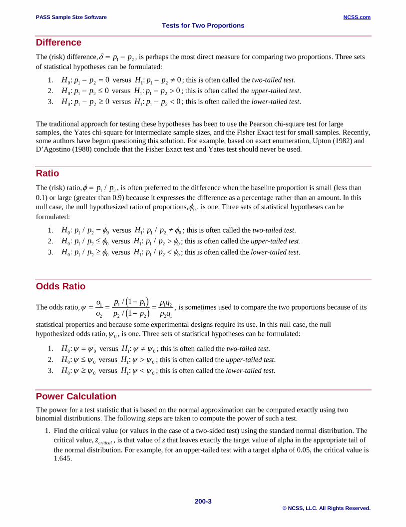
Difference The (risk) difference,δ = −p p1 2 , is perhaps the most direct measure for comparing two proportions. Three sets of statistical hypotheses can be formulated:

1. H p p0 1 2 0: − = versus H p p1 1 2 0: − ≠ ; this is often called the two-tailed test. 2. H p p0 1 2 0: − ≤ versus H p p1 1 2 0: − > ; this is often called the upper-tailed test. 3. H p p0 1 2 0: − ≥ versus H p p1 1 2 0: − < ; this is often called the lower-tailed test.

The traditional approach for testing these hypotheses has been to use the Pearson chi-square test for large samples, the Yates chi-square for intermediate sample sizes, and the Fisher Exact test for small samples. Recently, some authors have begun questioning this solution. For example, based on exact enumeration, Upton (1982) and D’Agostino (1988) conclude that the Fisher Exact test and Yates test should never be used.

Ratio The (risk) ratio,φ = p p1 2/ , is often preferred to the difference when the baseline proportion is small (less than 0.1) or large (greater than 0.9) because it expresses the difference as a percentage rather than an amount. In this null case, the null hypothesized ratio of proportions,φ0 , is one. Three sets of statistical hypotheses can be formulated:

1. versus ; this is often called the two-tailed test. 2. versus ; this is often called the upper-tailed test. 3. versus ; this is often called the lower-tailed test.

Odds Ratio

The odds ratio,( )( )

ψ = =−−

=oo

p pp p

p qp q

1

2

1 1

2 2

1 2

2 1

11

//

, is sometimes used to compare the two proportions because of its

statistical properties and because some experimental designs require its use. In this null case, the null hypothesized odds ratio,ψ 0 , is one. Three sets of statistical hypotheses can be formulated:

1. versus ; this is often called the two-tailed test. 2. versus ; this is often called the upper-tailed test. 3. versus ; this is often called the lower-tailed test.

Power Calculation The power for a test statistic that is based on the normal approximation can be computed exactly using two binomial distributions. The following steps are taken to compute the power of such a test.

1. Find the critical value (or values in the case of a two-sided test) using the standard normal distribution. The critical value, zcritical , is that value of z that leaves exactly the target value of alpha in the appropriate tail of the normal distribution. For example, for an upper-tailed test with a target alpha of 0.05, the critical value is 1.645.

H p p0 1 2 0: / = φ H p p1 1 2 0: / ≠ φH p p0 1 2 0: / ≤ φ H p p1 1 2 0: / > φH p p0 1 2 0: / ≥ φ H p p1 1 2 0: / < φ

H0 0:ψ ψ= H1 0:ψ ψ≠H0 0:ψ ψ≤ H1 0:ψ ψ>H0 0:ψ ψ≥ H1 0:ψ ψ<



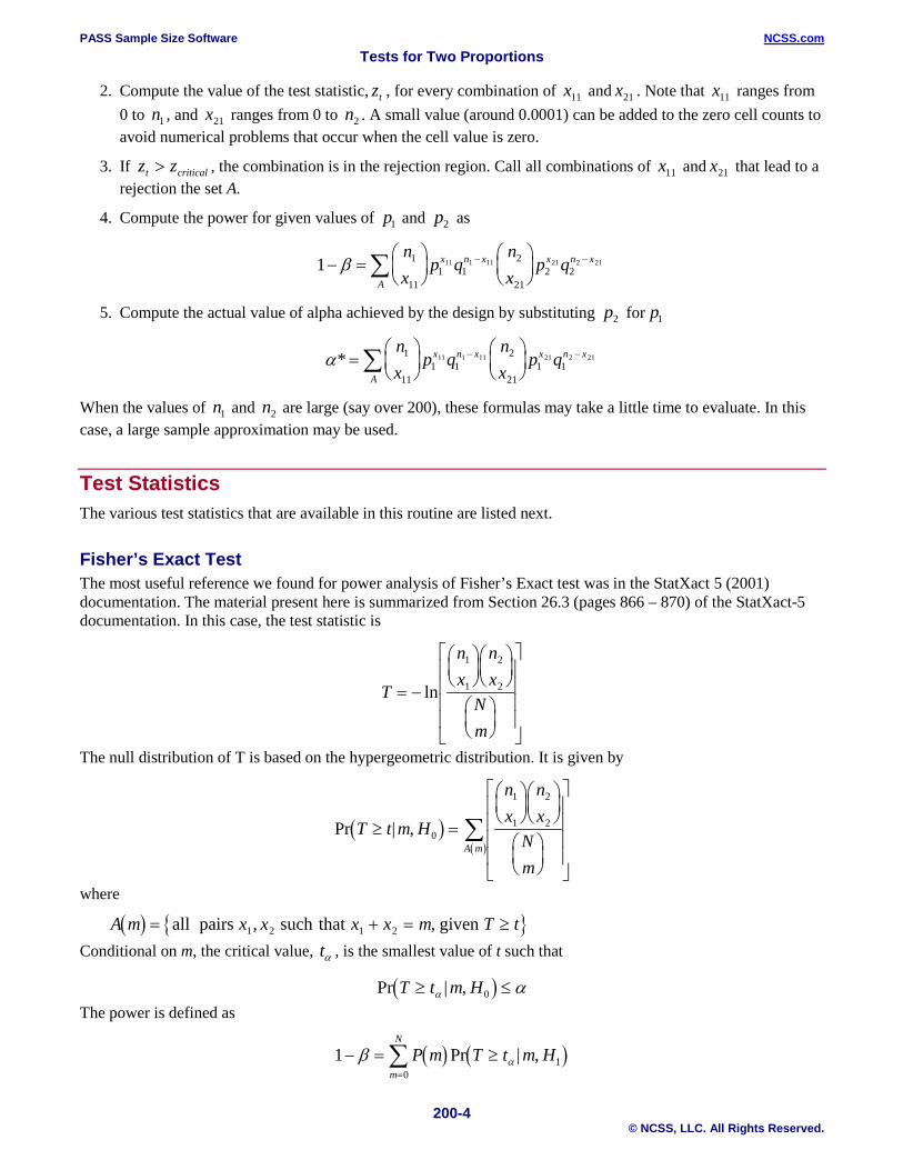
2. Compute the value of the test statistic, zt , for every combination of x11 and x21 . Note that x11 ranges from 0 to n1 , and x21 ranges from 0 to n2 . A small value (around 0.0001) can be added to the zero cell counts to avoid numerical problems that occur when the cell value is zero.

3. If z zt critical> , the combination is in the rejection region. Call all combinations of x11 and x21 that lead to a rejection the set A.

4. Compute the power for given values of p1 and p2 as

1 1

111 1

2

212 2

11 1 11 21 2 21− =

− −∑β

nx

p qnx

p qx n x x n x

A

5. Compute the actual value of alpha achieved by the design by substituting p2 for p1

α* =

− −∑

nx

p qnx

p qx n x x n x

A

1

111 1

2

211 1

11 1 11 21 2 21

When the values of n1 and n2 are large (say over 200), these formulas may take a little time to evaluate. In this case, a large sample approximation may be used.

Test Statistics The various test statistics that are available in this routine are listed next.

Fisher’s Exact Test The most useful reference we found for power analysis of Fisher’s Exact test was in the StatXact 5 (2001) documentation. The material present here is summarized from Section 26.3 (pages 866 – 870) of the StatXact-5 documentation. In this case, the test statistic is

The null distribution of T is based on the hypergeometric distribution. It is given by

( )( )

Pr | ,T t m H

nx

nx

Nm

A m

≥ =

∑0

1

1

2

2

where

( ) { }A m x x x x m T t= + = ≥all pairs such that given1 2 1 2, , Conditional on m, the critical value, αt , is the smallest value of t such that

( )Pr | ,T t m H≥ ≤α α0 The power is defined as

( ) ( )10

1− = ≥=∑β αP m T t m Hm

N

Pr | ,

T

nx

nx

Nm

= −

ln

1

1

2

2



where

( ) ( ) ( )( ) ( )

( )( )

Pr | ,, , , ,

, , , ,,

T t m Hb x n p b x n p

b x n p b x n pA m

A m T t

≥ =

∑∑

≥α

α

11 1 1 2 2 2

1 1 1 2 2 2

( ) ( )( ) ( )

P m x x m H

b x n p b x n p

= + =

=

Pr |

, , , ,1 2 1

1 1 1 2 2 2

( ) ( )b x n pnx

p px n x, , = − −1

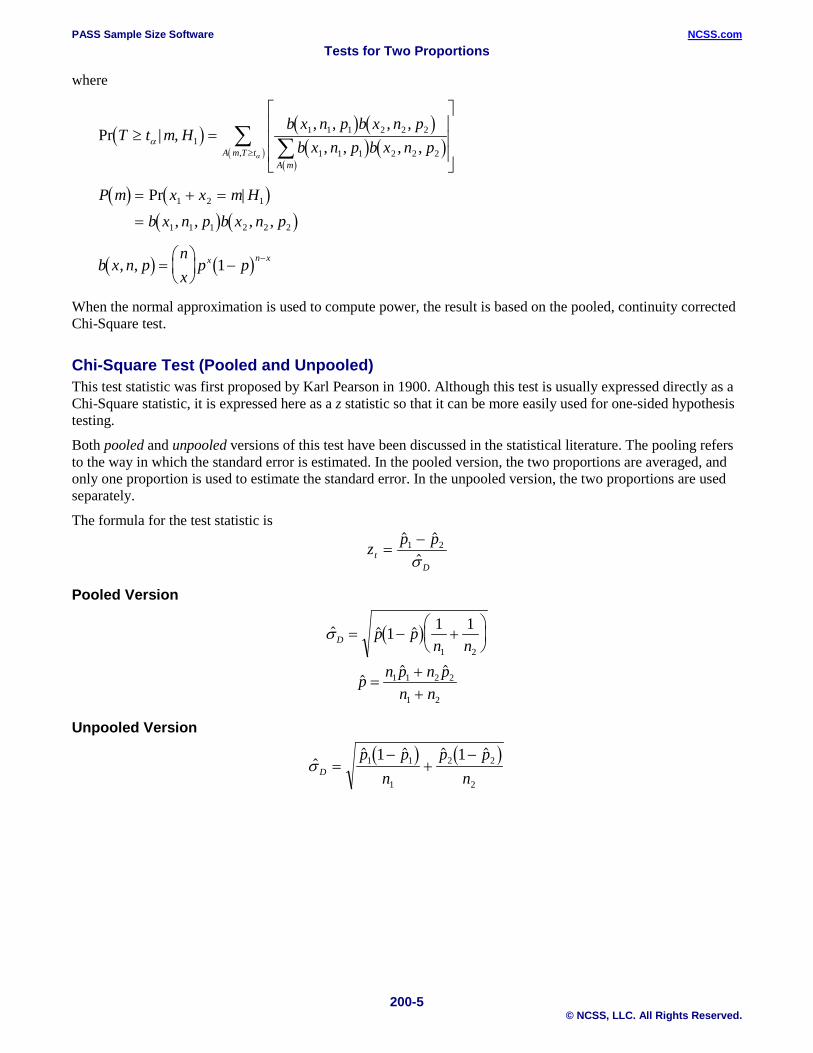
When the normal approximation is used to compute power, the result is based on the pooled, continuity corrected Chi-Square test.

Chi-Square Test (Pooled and Unpooled) This test statistic was first proposed by Karl Pearson in 1900. Although this test is usually expressed directly as a Chi-Square statistic, it is expressed here as a z statistic so that it can be more easily used for one-sided hypothesis testing.

Both pooled and unpooled versions of this test have been discussed in the statistical literature. The pooling refers to the way in which the standard error is estimated. In the pooled version, the two proportions are averaged, and only one proportion is used to estimate the standard error. In the unpooled version, the two proportions are used separately.

The formula for the test statistic is

z p pt

D

=−

1 2

σ

Pooled Version

( ) σD p pn n

= − +

1 1 1

1 2

Unpooled Version

( ) ( )

σD

p pn

p pn

=−

+−1 1

1

2 2

2

1 1

p n p n pn n

=++

1 1 2 2

1 2



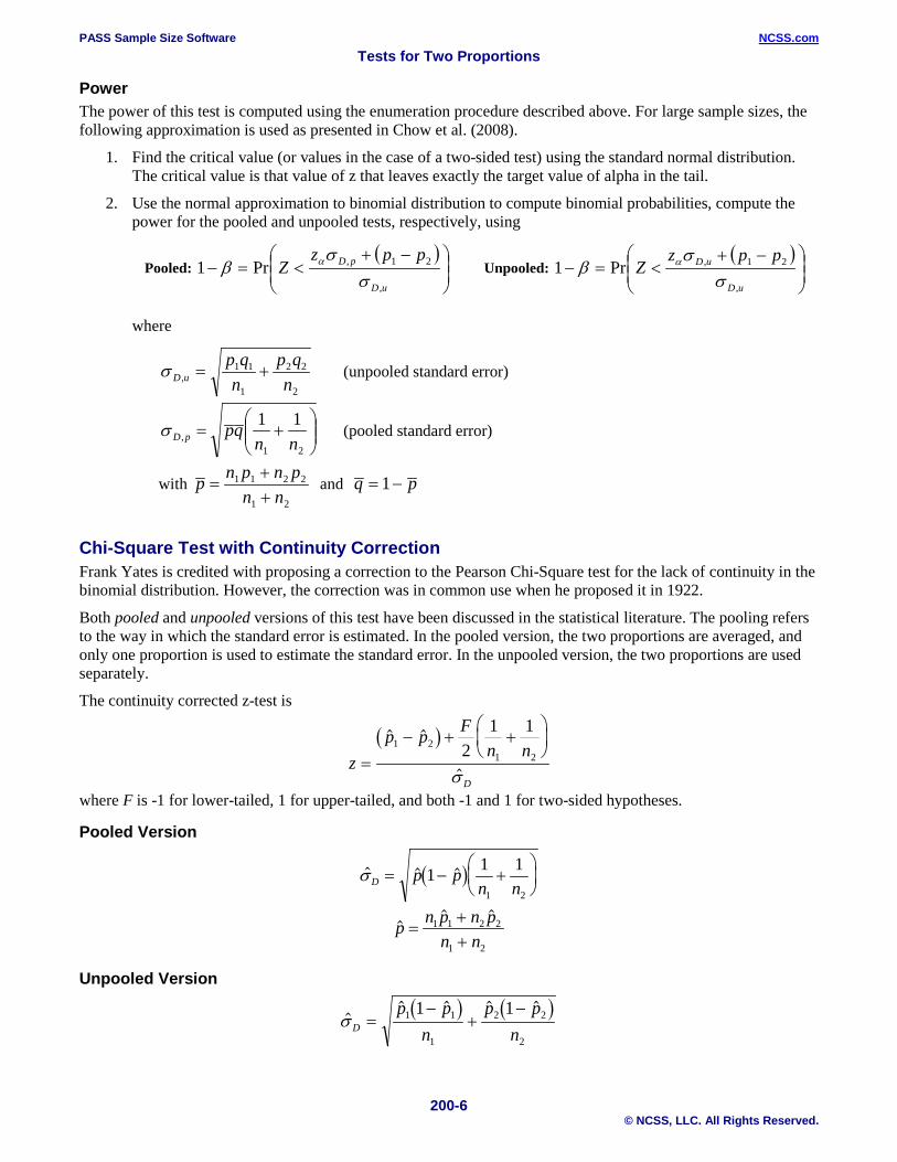
Power The power of this test is computed using the enumeration procedure described above. For large sample sizes, the following approximation is used as presented in Chow et al. (2008).

1. Find the critical value (or values in the case of a two-sided test) using the standard normal distribution. The critical value is that value of z that leaves exactly the target value of alpha in the tail.

2. Use the normal approximation to binomial distribution to compute binomial probabilities, compute the power for the pooled and unpooled tests, respectively, using

Pooled: ( )

−+<=−

uD

pD ppzZ

,

21,Pr1σ

σβ α Unpooled:

( )

−+<=−

uD

uD ppzZ

,

21,Pr1σ

σβ α

where

2

22

1

11, n

qpnqp

uD +=σ (unpooled standard error)

+=

21,

11nn

qppDσ (pooled standard error)

with 21

2211

nnpnpnp

++

= and pq −= 1

Chi-Square Test with Continuity Correction Frank Yates is credited with proposing a correction to the Pearson Chi-Square test for the lack of continuity in the binomial distribution. However, the correction was in common use when he proposed it in 1922.

Both pooled and unpooled versions of this test have been discussed in the statistical literature. The pooling refers to the way in which the standard error is estimated. In the pooled version, the two proportions are averaged, and only one proportion is used to estimate the standard error. In the unpooled version, the two proportions are used separately.

The continuity corrected z-test is

( )z

p p Fn n

D

=− + +

1 21 22

1 1

σ

where F is -1 for lower-tailed, 1 for upper-tailed, and both -1 and 1 for two-sided hypotheses.

Pooled Version

( ) σD p pn n

= − +

1 1 1

1 2

Unpooled Version

( ) ( )

σD

p pn

p pn

=−

+−1 1

1

2 2

2

1 1

p n p n pn n

=++

1 1 2 2

1 2



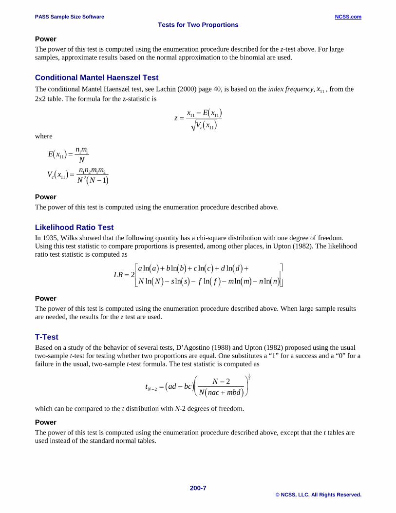
Power The power of this test is computed using the enumeration procedure described for the z-test above. For large samples, approximate results based on the normal approximation to the binomial are used.

Conditional Mantel Haenszel Test The conditional Mantel Haenszel test, see Lachin (2000) page 40, is based on the index frequency, , from the 2x2 table. The formula for the z-statistic is

where

Power The power of this test is computed using the enumeration procedure described above.

Likelihood Ratio Test In 1935, Wilks showed that the following quantity has a chi-square distribution with one degree of freedom. Using this test statistic to compare proportions is presented, among other places, in Upton (1982). The likelihood ratio test statistic is computed as

Power The power of this test is computed using the enumeration procedure described above. When large sample results are needed, the results for the z test are used.

T-Test Based on a study of the behavior of several tests, D’Agostino (1988) and Upton (1982) proposed using the usual two-sample t-test for testing whether two proportions are equal. One substitutes a “1” for a success and a “0” for a failure in the usual, two-sample t-test formula. The test statistic is computed as

which can be compared to the t distribution with N-2 degrees of freedom.

Power The power of this test is computed using the enumeration procedure described above, except that the t tables are used instead of the standard normal tables.

x11

( )( )

zx E x

V xc

=−11 11

11

( )E x n mN111 1=

( ) ( )V x n n m m

N Nc 111 2 1 22 1

=−

( ) ( ) ( ) ( )( ) ( ) ( ) ( ) ( )

LRa a b b c c d d

N N s s f f m m n n=

+ + + +

− − − −

2ln ln ln ln

ln ln ln ln ln

( ) ( )t ad bc N

N nac mbdN − = −−+

2

212



Procedure Options This section describes the options that are specific to this procedure. These are located on the Design tab. For more information about the options of other tabs, go to the Procedure Window chapter.

Design Tab The Design tab contains the parameters associated with this test such as the proportions, sample sizes, alpha, and power.

Solve For

Solve For This option specifies the parameter to be solved for using the other parameters. The parameters that may be selected are Power, Sample Size, and Effect Sieze. Under most situations, you will select either Power or Sample Size.

Select Power when you want to calculate the power of an experiment.

Select Sample Size when you want to calculate the sample size needed to achieve a given power and alpha level.

Power Calculation

Power Calculation Method Select the method to be used to calculate power. When the sample sizes are reasonably large (i.e. greater than 50) and the proportions are between 0.2 and 0.8 the two methods will give similar results. For smaller sample sizes and more extreme proportions (less than 0.2 or greater than 0.8), the normal approximation is not as accurate so the binomial calculations may be more appropriate.

The choices are

• Binomial Enumeration Power for each test is computed using binomial enumeration of all possible outcomes when N1 and N2 ≤ Maximum N1 or N2 for Binomial Enumeration (otherwise, the normal approximation is used). Binomial enumeration of all outcomes is possible because of the discrete nature of the data.

• Normal Approximation Approximate power for each test is computed using the normal approximation to the binomial distribution.

Actual alpha values are only computed when “Binomial Enumeration” is selected.

Power Calculation – Binomial Enumeration Options Only shown when Power Calculation Method = “Binomial Enumeration”

Maximum N1 or N2 for Binomial Enumeration When both N1 and N2 are less than or equal to this amount, power calculations using the binomial distribution are made. The value of the “Actual Alpha” is only calculated when binomial power calculations are made. When either N1 or N2 is larger than this amount, the normal approximation to the binomial is used for power calculations.



Zero Count Adjustment Method Zero cell counts cause many calculation problems when enumerating binomial probabilities. To compensate for this, a small value (called the “Zero Count Adjustment Value”) may be added either to all cells or to all cells with zero counts. This option specifies which type of adjustment you want to use.

Adding a small value is controversial, but may be necessary. Some statisticians recommend adding 0.5 while others recommend 0.25. We have found that adding values as small as 0.0001 seems to work well.

Zero Count Adjustment Value Zero cell counts cause many calculation problems when enumerating binomial probabilities. To compensate for this, a small value may be added either to all cells or to all zero cells. This is the amount that is added. We have found that 0.0001 works well.

Be warned that the value of the ratio and the odds ratio will be affected by the amount specified here!

Test

Alternative Hypothesis Specify whether the alternative hypothesis of the test is one-sided or two-sided. If a one-sided test is chosen, the hypothesis test direction is chosen based on whether P1 is greater than or less than P2.

• Two-Sided Hypothesis Test 𝐻𝐻0:𝑃𝑃1 = 𝑃𝑃2 vs. 𝐻𝐻1:𝑃𝑃1 ≠ 𝑃𝑃2

• One-Sided Hypothesis Tests Upper: 𝐻𝐻0:𝑃𝑃1 ≤ 𝑃𝑃2 vs. 𝐻𝐻1:𝑃𝑃1 > 𝑃𝑃2

Lower: 𝐻𝐻0:𝑃𝑃1 ≥ 𝑃𝑃2 vs. 𝐻𝐻1:𝑃𝑃1 < 𝑃𝑃2

Test Type Specify which test statistic will be used in searching and reporting.

Note that “C.C.” is an abbreviation for Continuity Correction. This refers to the adding or subtracting 2/(N1+N2) to (or from) the numerator of the z-value to bring the normal approximation closer to the binomial distribution.

Power and Alpha

Power This option specifies one or more values for power. Power is the probability of rejecting a false null hypothesis, and is equal to one minus Beta. Beta is the probability of a type-II error, which occurs when a false null hypothesis is not rejected. In this procedure, a type-II error occurs when you fail to reject the null hypothesis of equal proportions when in fact they are different.

Values must be between zero and one. Historically, the value of 0.80 (Beta = 0.20) was used for power. Now, 0.90 (Beta = 0.10) is also commonly used.

A single value may be entered here or a range of values such as 0.8 to 0.95 by 0.05 may be entered.



Alpha This option specifies one or more values for the probability of a type-I error. A type-I error occurs when a true null hypothesis is rejected. For this procedure, a type-I error occurs when you reject the null hypothesis of equal proportions when in fact they are equal.

Values must be between zero and one. Historically, the value of 0.05 has been used for alpha. This means that about one test in twenty will falsely reject the null hypothesis. You should pick a value for alpha that represents the risk of a type-I error you are willing to take in your experimental situation.

You may enter a range of values such as 0.01 0.05 0.10 or 0.01 to 0.10 by 0.01.

Sample Size (When Solving for Sample Size)

Group Allocation Select the option that describes the constraints on N1 or N2 or both.

The options are

• Equal (N1 = N2) This selection is used when you wish to have equal sample sizes in each group. Since you are solving for both sample sizes at once, no additional sample size parameters need to be entered.

• Enter N1, solve for N2 Select this option when you wish to fix N1 at some value (or values), and then solve only for N2. Please note that for some values of N1, there may not be a value of N2 that is large enough to obtain the desired power.

• Enter N2, solve for N1 Select this option when you wish to fix N2 at some value (or values), and then solve only for N1. Please note that for some values of N2, there may not be a value of N1 that is large enough to obtain the desired power.

• Enter R = N2/N1, solve for N1 and N2 For this choice, you set a value for the ratio of N2 to N1, and then PASS determines the needed N1 and N2, with this ratio, to obtain the desired power. An equivalent representation of the ratio, R, is

N2 = R * N1.

• Enter percentage in Group 1, solve for N1 and N2 For this choice, you set a value for the percentage of the total sample size that is in Group 1, and then PASS determines the needed N1 and N2 with this percentage to obtain the desired power.

N1 (Sample Size, Group 1) This option is displayed if Group Allocation = “Enter N1, solve for N2”

N1 is the number of items or individuals sampled from the Group 1 population.

N1 must be ≥ 2. You can enter a single value or a series of values.

N2 (Sample Size, Group 2) This option is displayed if Group Allocation = “Enter N2, solve for N1”





R (Group Sample Size Ratio) This option is displayed only if Group Allocation = “Enter R = N2/N1, solve for N1 and N2.”

R is the ratio of N2 to N1. That is,

R = N2 / N1.

Use this value to fix the ratio of N2 to N1 while solving for N1 and N2. Only sample size combinations with this ratio are considered.

N2 is related to N1 by the formula:

N2 = [R × N1],

where the value [Y] is the next integer ≥ Y.

For example, setting R = 2.0 results in a Group 2 sample size that is double the sample size in Group 1 (e.g., N1 = 10 and N2 = 20, or N1 = 50 and N2 = 100).

R must be greater than 0. If R < 1, then N2 will be less than N1; if R > 1, then N2 will be greater than N1. You can enter a single or a series of values.

Percent in Group 1 This option is displayed only if Group Allocation = “Enter percentage in Group 1, solve for N1 and N2.”

Use this value to fix the percentage of the total sample size allocated to Group 1 while solving for N1 and N2. Only sample size combinations with this Group 1 percentage are considered. Small variations from the specified percentage may occur due to the discrete nature of sample sizes.

The Percent in Group 1 must be greater than 0 and less than 100. You can enter a single or a series of values.

Sample Size (When Not Solving for Sample Size)

Group Allocation Select the option that describes how individuals in the study will be allocated to Group 1 and to Group 2.

The options are

• Equal (N1 = N2) This selection is used when you wish to have equal sample sizes in each group. A single per group sample size will be entered.

• Enter N1 and N2 individually This choice permits you to enter different values for N1 and N2.

• Enter N1 and R, where N2 = R * N1 Choose this option to specify a value (or values) for N1, and obtain N2 as a ratio (multiple) of N1.

• Enter total sample size and percentage in Group 1 Choose this option to specify a value (or values) for the total sample size (N), obtain N1 as a percentage of N, and then N2 as N - N1.



Sample Size Per Group This option is displayed only if Group Allocation = “Equal (N1 = N2).”

The Sample Size Per Group is the number of items or individuals sampled from each of the Group 1 and Group 2 populations. Since the sample sizes are the same in each group, this value is the value for N1, and also the value for N2.

The Sample Size Per Group must be ≥ 2. You can enter a single value or a series of values.

N1 (Sample Size, Group 1) This option is displayed if Group Allocation = “Enter N1 and N2 individually” or “Enter N1 and R, where N2 = R * N1.”



N2 (Sample Size, Group 2) This option is displayed only if Group Allocation = “Enter N1 and N2 individually.”



R (Group Sample Size Ratio) This option is displayed only if Group Allocation = “Enter N1 and R, where N2 = R * N1.”

R is the ratio of N2 to N1. That is,

R = N2/N1

Use this value to obtain N2 as a multiple (or proportion) of N1.

N2 is calculated from N1 using the formula:

N2=[R x N1],

where the value [Y] is the next integer ≥ Y.

For example, setting R = 2.0 results in a Group 2 sample size that is double the sample size in Group 1.

R must be greater than 0. If R < 1, then N2 will be less than N1; if R > 1, then N2 will be greater than N1. You can enter a single value or a series of values.

Total Sample Size (N) This option is displayed only if Group Allocation = “Enter total sample size and percentage in Group 1.”

This is the total sample size, or the sum of the two group sample sizes. This value, along with the percentage of the total sample size in Group 1, implicitly defines N1 and N2.

The total sample size must be greater than one, but practically, must be greater than 3, since each group sample size needs to be at least 2.

You can enter a single value or a series of values.

Percent in Group 1 This option is displayed only if Group Allocation = “Enter total sample size and percentage in Group 1.”

This value fixes the percentage of the total sample size allocated to Group 1. Small variations from the specified percentage may occur due to the discrete nature of sample sizes.

The Percent in Group 1 must be greater than 0 and less than 100. You can enter a single value or a series of values.



Effect Size

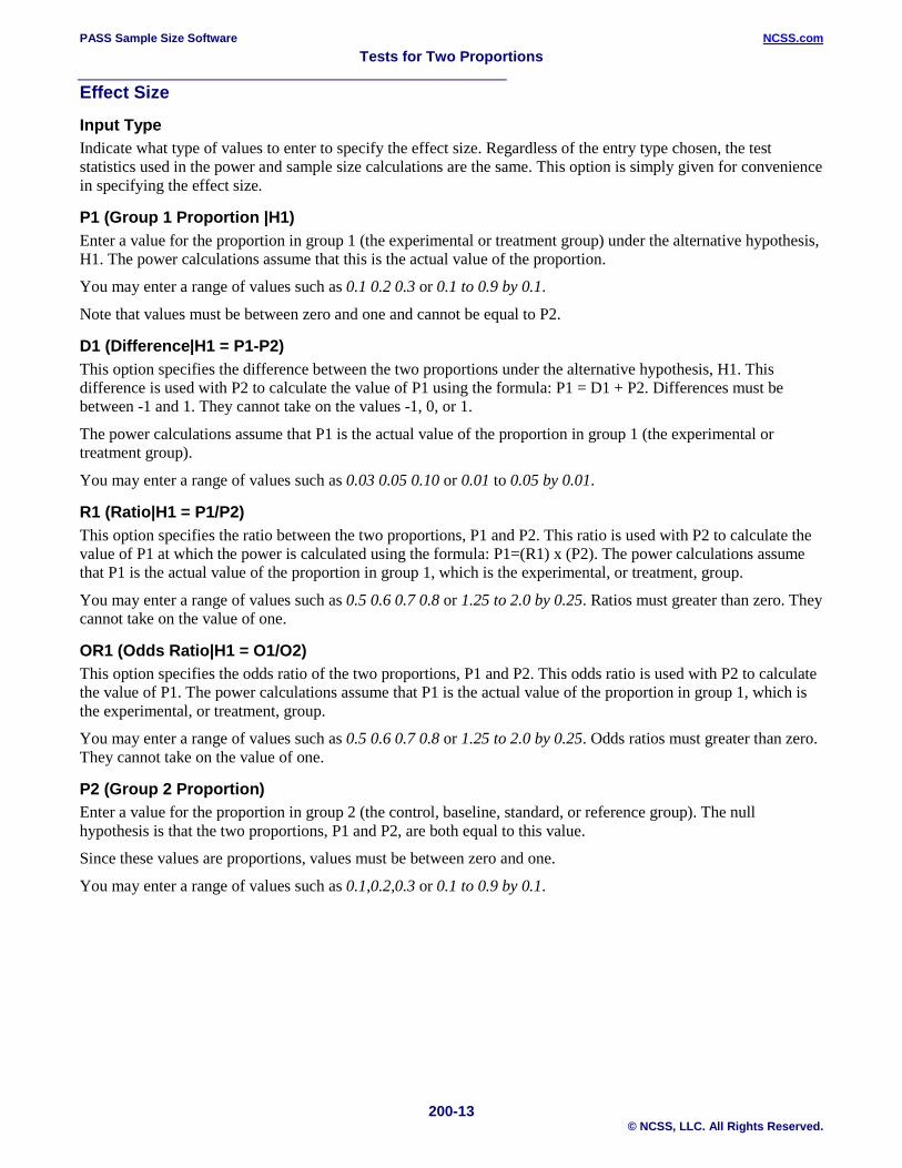
Input Type Indicate what type of values to enter to specify the effect size. Regardless of the entry type chosen, the test statistics used in the power and sample size calculations are the same. This option is simply given for convenience in specifying the effect size.

P1 (Group 1 Proportion |H1) Enter a value for the proportion in group 1 (the experimental or treatment group) under the alternative hypothesis, H1. The power calculations assume that this is the actual value of the proportion.


Note that values must be between zero and one and cannot be equal to P2.

D1 (Difference|H1 = P1-P2) This option specifies the difference between the two proportions under the alternative hypothesis, H1. This difference is used with P2 to calculate the value of P1 using the formula: P1 = D1 + P2. Differences must be between -1 and 1. They cannot take on the values -1, 0, or 1.

The power calculations assume that P1 is the actual value of the proportion in group 1 (the experimental or treatment group).


R1 (Ratio|H1 = P1/P2) This option specifies the ratio between the two proportions, P1 and P2. This ratio is used with P2 to calculate the value of P1 at which the power is calculated using the formula: P1=(R1) x (P2). The power calculations assume that P1 is the actual value of the proportion in group 1, which is the experimental, or treatment, group.

You may enter a range of values such as 0.5 0.6 0.7 0.8 or 1.25 to 2.0 by 0.25. Ratios must greater than zero. They cannot take on the value of one.

OR1 (Odds Ratio|H1 = O1/O2) This option specifies the odds ratio of the two proportions, P1 and P2. This odds ratio is used with P2 to calculate the value of P1. The power calculations assume that P1 is the actual value of the proportion in group 1, which is the experimental, or treatment, group.

You may enter a range of values such as 0.5 0.6 0.7 0.8 or 1.25 to 2.0 by 0.25. Odds ratios must greater than zero. They cannot take on the value of one.

P2 (Group 2 Proportion) Enter a value for the proportion in group 2 (the control, baseline, standard, or reference group). The null hypothesis is that the two proportions, P1 and P2, are both equal to this value.

Since these values are proportions, values must be between zero and one.

You may enter a range of values such as 0.1,0.2,0.3 or 0.1 to 0.9 by 0.1.



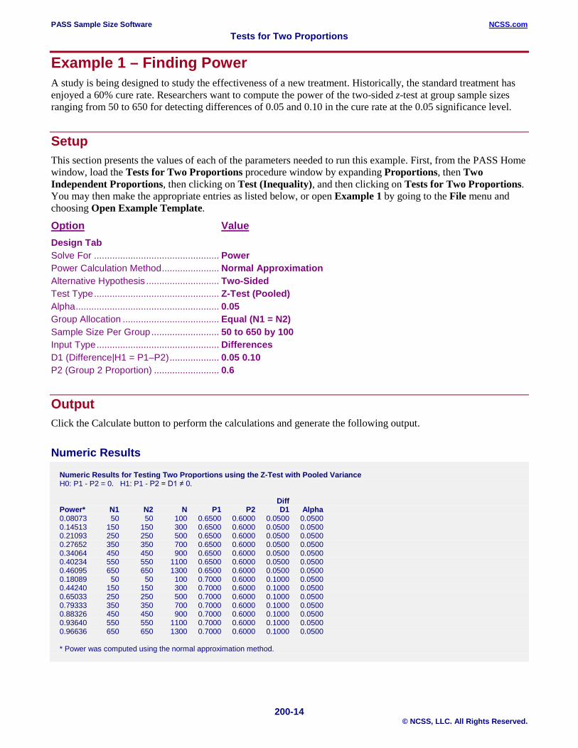
Example 1 – Finding Power A study is being designed to study the effectiveness of a new treatment. Historically, the standard treatment has enjoyed a 60% cure rate. Researchers want to compute the power of the two-sided z-test at group sample sizes ranging from 50 to 650 for detecting differences of 0.05 and 0.10 in the cure rate at the 0.05 significance level.

Setup This section presents the values of each of the parameters needed to run this example. First, from the PASS Home window, load the Tests for Two Proportions procedure window by expanding Proportions, then Two Independent Proportions, then clicking on Test (Inequality), and then clicking on Tests for Two Proportions. You may then make the appropriate entries as listed below, or open Example 1 by going to the File menu and choosing Open Example Template.

Option Value Design Tab Solve For ................................................ Power Power Calculation Method ...................... Normal Approximation Alternative Hypothesis ............................ Two-Sided Test Type ................................................ Z-Test (Pooled) Alpha ....................................................... 0.05 Group Allocation ..................................... Equal (N1 = N2) Sample Size Per Group .......................... 50 to 650 by 100 Input Type ............................................... Differences D1 (Difference|H1 = P1–P2) ................... 0.05 0.10 P2 (Group 2 Proportion) ......................... 0.6

Output Click the Calculate button to perform the calculations and generate the following output.

Numeric Results

Numeric Results for Testing Two Proportions using the Z-Test with Pooled Variance H0: P1 - P2 = 0. H1: P1 - P2 = D1 ≠ 0. Diff Power* N1 N2 N P1 P2 D1 Alpha 0.08073 50 50 100 0.6500 0.6000 0.0500 0.0500 0.14513 150 150 300 0.6500 0.6000 0.0500 0.0500 0.21093 250 250 500 0.6500 0.6000 0.0500 0.0500 0.27652 350 350 700 0.6500 0.6000 0.0500 0.0500 0.34064 450 450 900 0.6500 0.6000 0.0500 0.0500 0.40234 550 550 1100 0.6500 0.6000 0.0500 0.0500 0.46095 650 650 1300 0.6500 0.6000 0.0500 0.0500 0.18089 50 50 100 0.7000 0.6000 0.1000 0.0500 0.44240 150 150 300 0.7000 0.6000 0.1000 0.0500 0.65033 250 250 500 0.7000 0.6000 0.1000 0.0500 0.79333 350 350 700 0.7000 0.6000 0.1000 0.0500 0.88326 450 450 900 0.7000 0.6000 0.1000 0.0500 0.93640 550 550 1100 0.7000 0.6000 0.1000 0.0500 0.96636 650 650 1300 0.7000 0.6000 0.1000 0.0500 * Power was computed using the normal approximation method.



References Chow, S.C., Shao, J., and Wang, H. 2008. Sample Size Calculations in Clinical Research, Second Edition. Chapman & Hall/CRC. Boca Raton, Florida. D'Agostino, R.B., Chase, W., and Belanger, A. 1988.'The Appropriateness of Some Common Procedures for Testing the Equality of Two Independent Binomial Populations', The American Statistician, August 1988, Volume 42 Number 3, pages 198-202. Fleiss, J. L., Levin, B., and Paik, M.C. 2003. Statistical Methods for Rates and Proportions. Third Edition. John Wiley & Sons. New York. Lachin, John M. 2000. Biostatistical Methods. John Wiley & Sons. New York. Machin, D., Campbell, M., Fayers, P., and Pinol, A. 1997. Sample Size Tables for Clinical Studies, 2nd Edition. Blackwell Science. Malden, Mass. Ryan, Thomas P. 2013. Sample Size Determination and Power. John Wiley & Sons. Hoboken, New Jersey. Report Definitions Power is the probability of rejecting a false null hypothesis. N1 and N2 are the number of items sampled from each population. N is the total sample size, N1 + N2. P1 is the proportion for Group 1 at which power and sample size calculations are made. This is the treatment or experimental group. P2 is the proportion for Group 2. This is the standard, reference, or control group. D1 is the difference P1 - P2 assumed for power and sample size calcualtions. Alpha is the probability of rejecting a true null hypothesis. Summary Statements Group sample sizes of 50 in group 1 and 50 in group 2 achieve 8.073% power to detect a difference between the group proportions of 0.0500. The proportion in group 1 (the treatment group) is assumed to be 0.6000 under the null hypothesis and 0.6500 under the alternative hypothesis. The proportion in group 2 (the control group) is 0.6000. The test statistic used is the two-sided Z-Test with pooled variance. The significance level of the test is 0.0500.

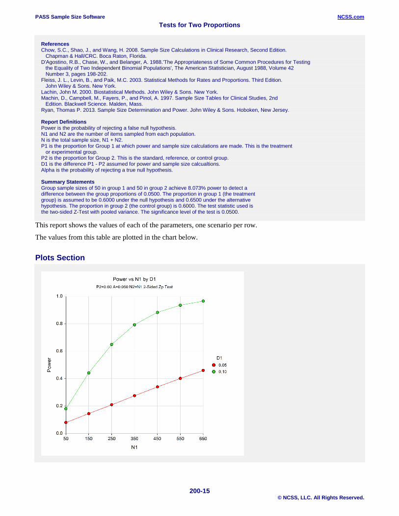
This report shows the values of each of the parameters, one scenario per row.

The values from this table are plotted in the chart below.

Plots Section



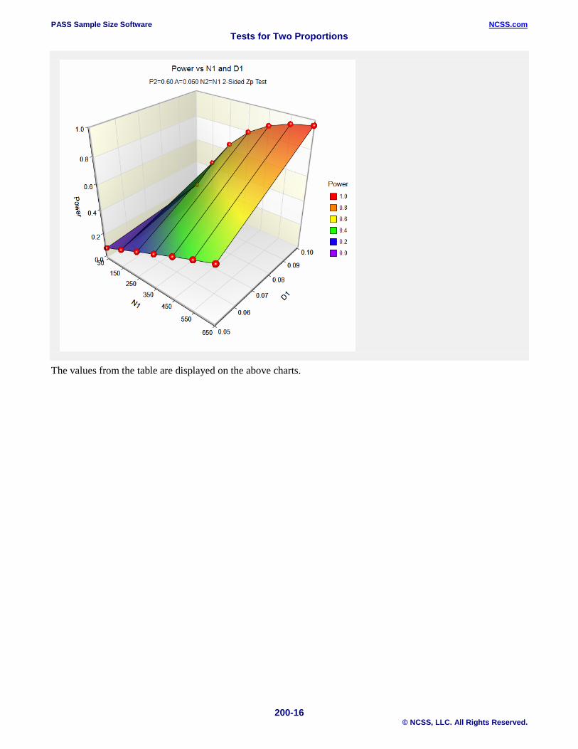
The values from the table are displayed on the above charts.



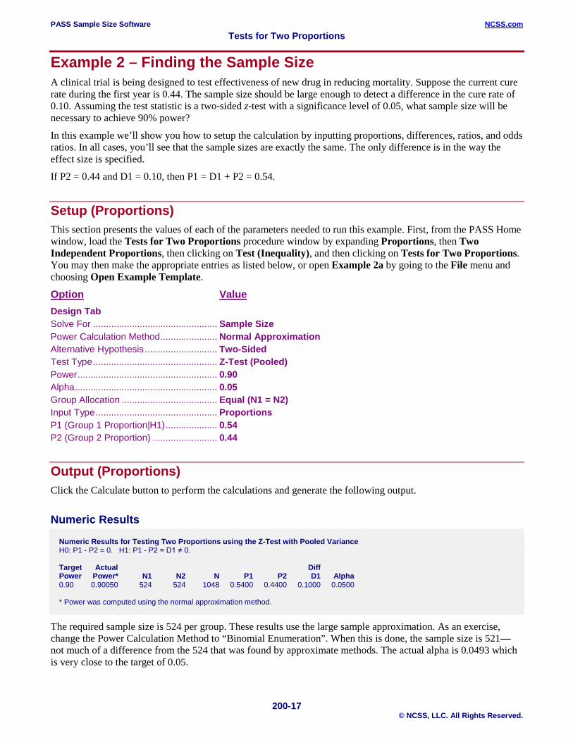
Example 2 – Finding the Sample Size A clinical trial is being designed to test effectiveness of new drug in reducing mortality. Suppose the current cure rate during the first year is 0.44. The sample size should be large enough to detect a difference in the cure rate of 0.10. Assuming the test statistic is a two-sided z-test with a significance level of 0.05, what sample size will be necessary to achieve 90% power?

In this example we’ll show you how to setup the calculation by inputting proportions, differences, ratios, and odds ratios. In all cases, you’ll see that the sample sizes are exactly the same. The only difference is in the way the effect size is specified.

If P2 = 0.44 and D1 = 0.10, then P1 = D1 + P2 = 0.54.

Setup (Proportions) This section presents the values of each of the parameters needed to run this example. First, from the PASS Home window, load the Tests for Two Proportions procedure window by expanding Proportions, then Two Independent Proportions, then clicking on Test (Inequality), and then clicking on Tests for Two Proportions. You may then make the appropriate entries as listed below, or open Example 2a by going to the File menu and choosing Open Example Template.

Option Value Design Tab Solve For ................................................ Sample Size Power Calculation Method ...................... Normal Approximation Alternative Hypothesis ............................ Two-Sided Test Type ................................................ Z-Test (Pooled) Power ...................................................... 0.90 Alpha ....................................................... 0.05 Group Allocation ..................................... Equal (N1 = N2) Input Type ............................................... Proportions P1 (Group 1 Proportion|H1) .................... 0.54 P2 (Group 2 Proportion) ......................... 0.44

Output (Proportions) Click the Calculate button to perform the calculations and generate the following output.

Numeric Results

Numeric Results for Testing Two Proportions using the Z-Test with Pooled Variance H0: P1 - P2 = 0. H1: P1 - P2 = D1 ≠ 0. Target Actual Diff Power Power* N1 N2 N P1 P2 D1 Alpha 0.90 0.90050 524 524 1048 0.5400 0.4400 0.1000 0.0500 * Power was computed using the normal approximation method.

The required sample size is 524 per group. These results use the large sample approximation. As an exercise, change the Power Calculation Method to “Binomial Enumeration”. When this is done, the sample size is 521—not much of a difference from the 524 that was found by approximate methods. The actual alpha is 0.0493 which is very close to the target of 0.05.



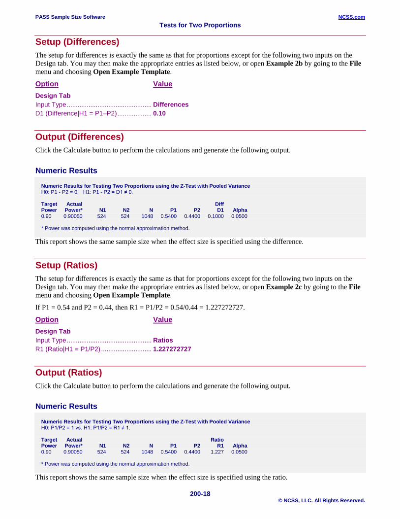
Setup (Differences) The setup for differences is exactly the same as that for proportions except for the following two inputs on the Design tab. You may then make the appropriate entries as listed below, or open Example 2b by going to the File menu and choosing Open Example Template.

Option Value Design Tab Input Type ............................................... Differences D1 (Difference|H1 = P1–P2) ................... 0.10

Output (Differences) Click the Calculate button to perform the calculations and generate the following output.

Numeric Results

Numeric Results for Testing Two Proportions using the Z-Test with Pooled Variance H0: P1 - P2 = 0. H1: P1 - P2 = D1 ≠ 0. Target Actual Diff Power Power* N1 N2 N P1 P2 D1 Alpha 0.90 0.90050 524 524 1048 0.5400 0.4400 0.1000 0.0500 * Power was computed using the normal approximation method.

This report shows the same sample size when the effect size is specified using the difference.

Setup (Ratios) The setup for differences is exactly the same as that for proportions except for the following two inputs on the Design tab. You may then make the appropriate entries as listed below, or open Example 2c by going to the File menu and choosing Open Example Template.

If P1 = 0.54 and P2 = 0.44, then R1 = P1/P2 = 0.54/0.44 = 1.227272727.

Option Value Design Tab Input Type ............................................... Ratios R1 (Ratio|H1 = P1/P2) ............................ 1.227272727

Output (Ratios) Click the Calculate button to perform the calculations and generate the following output.

Numeric Results

Numeric Results for Testing Two Proportions using the Z-Test with Pooled Variance H0: P1/P2 = 1 vs. H1: P1/P2 = R1 ≠ 1. Target Actual Ratio Power Power* N1 N2 N P1 P2 R1 Alpha 0.90 0.90050 524 524 1048 0.5400 0.4400 1.227 0.0500 * Power was computed using the normal approximation method.

This report shows the same sample size when the effect size is specified using the ratio.



Setup (Odds Ratios) The setup for differences is exactly the same as that for proportions except for the following two inputs on the Design tab. You may then make the appropriate entries as listed below, or open Example 2d by going to the File menu and choosing Open Example Template.

If P1 = 0.54 and P2 = 0.44, then OR1 = O1/O2 = [0.54/(1 – 0.54)]/[0.44(1 – 0.44)] = 1.494071146

Option Value Design Tab Input Type ............................................... Odds Ratios OR1 (Odds Ratio|H1 = O1/O2) ............... 1.494071146

Output (Odds Ratios) Click the Calculate button to perform the calculations and generate the following output.

Numeric Results

Numeric Results for Testing Two Proportions using the Z-Test with Pooled Variance H0: P1/P2 = 1 vs. H1: P1/P2 = R1 ≠ 1. Target Actual O.R. Power Power* N1 N2 N P1 P2 OR1 Alpha 0.90 0.90050 524 524 1048 0.5400 0.4400 1.494 0.0500 * Power was computed using the normal approximation method.

This report shows the same sample size when the effect size is specified using the odds ratio.



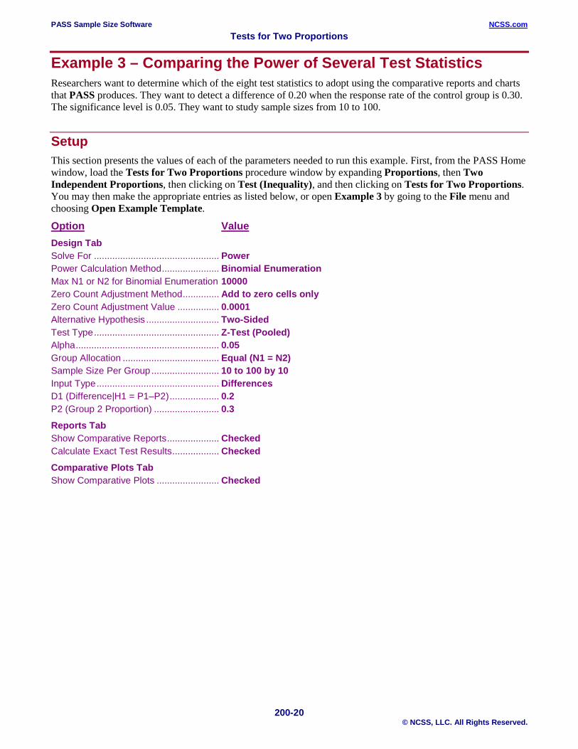
Example 3 – Comparing the Power of Several Test Statistics Researchers want to determine which of the eight test statistics to adopt using the comparative reports and charts that PASS produces. They want to detect a difference of 0.20 when the response rate of the control group is 0.30. The significance level is 0.05. They want to study sample sizes from 10 to 100.


Option Value Design Tab Solve For ................................................ Power Power Calculation Method ...................... Binomial Enumeration Max N1 or N2 for Binomial Enumeration 10000 Zero Count Adjustment Method .............. Add to zero cells only Zero Count Adjustment Value ................ 0.0001 Alternative Hypothesis ............................ Two-Sided Test Type ................................................ Z-Test (Pooled) Alpha ....................................................... 0.05 Group Allocation ..................................... Equal (N1 = N2) Sample Size Per Group .......................... 10 to 100 by 10 Input Type ............................................... Differences D1 (Difference|H1 = P1–P2) ................... 0.2 P2 (Group 2 Proportion) ......................... 0.3

Reports Tab Show Comparative Reports .................... Checked Calculate Exact Test Results .................. Checked Comparative Plots Tab Show Comparative Plots ........................ Checked




Numeric Results and Plots

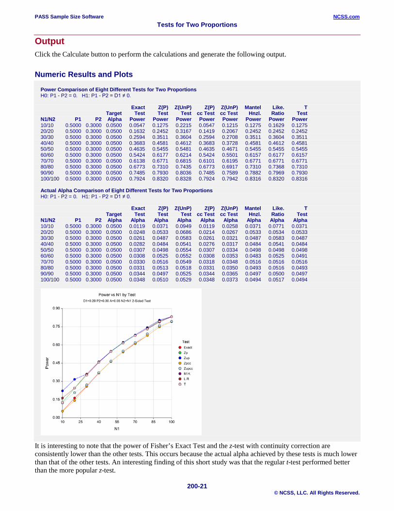
Power Comparison of Eight Different Tests for Two Proportions H0: P1 - P2 = 0. H1: P1 - P2 = D1 ≠ 0. Exact Z(P) Z(UnP) Z(P) Z(UnP) Mantel Like. T Target Test Test Test cc Test cc Test Hnzl. Ratio Test N1/N2 P1 P2 Alpha Power Power Power Power Power Power Power Power 10/10 0.5000 0.3000 0.0500 0.0547 0.1275 0.2215 0.0547 0.1215 0.1275 0.1629 0.1275 20/20 0.5000 0.3000 0.0500 0.1632 0.2452 0.3167 0.1419 0.2067 0.2452 0.2452 0.2452 30/30 0.5000 0.3000 0.0500 0.2594 0.3511 0.3604 0.2594 0.2708 0.3511 0.3604 0.3511 40/40 0.5000 0.3000 0.0500 0.3683 0.4581 0.4612 0.3683 0.3728 0.4581 0.4612 0.4581 50/50 0.5000 0.3000 0.0500 0.4635 0.5455 0.5481 0.4635 0.4671 0.5455 0.5455 0.5455 60/60 0.5000 0.3000 0.0500 0.5424 0.6177 0.6214 0.5424 0.5501 0.6157 0.6177 0.6157 70/70 0.5000 0.3000 0.0500 0.6138 0.6771 0.6815 0.6101 0.6195 0.6771 0.6771 0.6771 80/80 0.5000 0.3000 0.0500 0.6773 0.7310 0.7435 0.6773 0.6917 0.7310 0.7368 0.7310 90/90 0.5000 0.3000 0.0500 0.7485 0.7930 0.8036 0.7485 0.7589 0.7882 0.7969 0.7930 100/100 0.5000 0.3000 0.0500 0.7924 0.8320 0.8328 0.7924 0.7942 0.8316 0.8320 0.8316 Actual Alpha Comparison of Eight Different Tests for Two Proportions H0: P1 - P2 = 0. H1: P1 - P2 = D1 ≠ 0. Exact Z(P) Z(UnP) Z(P) Z(UnP) Mantel Like. T Target Test Test Test cc Test cc Test Hnzl. Ratio Test N1/N2 P1 P2 Alpha Alpha Alpha Alpha Alpha Alpha Alpha Alpha Alpha 10/10 0.5000 0.3000 0.0500 0.0119 0.0371 0.0949 0.0119 0.0258 0.0371 0.0771 0.0371 20/20 0.5000 0.3000 0.0500 0.0248 0.0533 0.0686 0.0214 0.0267 0.0533 0.0534 0.0533 30/30 0.5000 0.3000 0.0500 0.0261 0.0487 0.0583 0.0261 0.0321 0.0487 0.0583 0.0487 40/40 0.5000 0.3000 0.0500 0.0282 0.0484 0.0541 0.0276 0.0317 0.0484 0.0541 0.0484 50/50 0.5000 0.3000 0.0500 0.0307 0.0498 0.0554 0.0307 0.0334 0.0498 0.0498 0.0498 60/60 0.5000 0.3000 0.0500 0.0308 0.0525 0.0552 0.0308 0.0353 0.0483 0.0525 0.0491 70/70 0.5000 0.3000 0.0500 0.0330 0.0516 0.0549 0.0318 0.0348 0.0516 0.0516 0.0516 80/80 0.5000 0.3000 0.0500 0.0331 0.0513 0.0518 0.0331 0.0350 0.0493 0.0516 0.0493 90/90 0.5000 0.3000 0.0500 0.0344 0.0497 0.0525 0.0344 0.0365 0.0497 0.0500 0.0497 100/100 0.5000 0.3000 0.0500 0.0348 0.0510 0.0529 0.0348 0.0373 0.0494 0.0517 0.0494

It is interesting to note that the power of Fisher’s Exact Test and the z-test with continuity correction are consistently lower than the other tests. This occurs because the actual alpha achieved by these tests is much lower than that of the other tests. An interesting finding of this short study was that the regular t-test performed better than the more popular z-test.



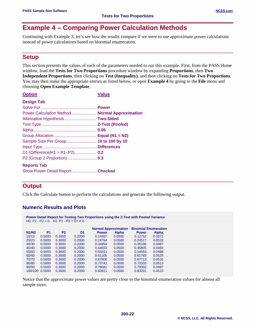
Example 4 – Comparing Power Calculation Methods Continuing with Example 3, let’s see how the results compare if we were to use approximate power calculations instead of power calculations based on binomial enumeration.


Option Value Design Tab Solve For ................................................ Power Power Calculation Method ...................... Normal Approximation Alternative Hypothesis ............................ Two-Sided Test Type ................................................ Z-Test (Pooled) Alpha ....................................................... 0.05 Group Allocation ..................................... Equal (N1 = N2) Sample Size Per Group .......................... 10 to 100 by 10 Input Type ............................................... Differences D1 (Difference|H1 = P1–P2) ................... 0.2 P2 (Group 2 Proportion) ......................... 0.3

Reports Tab Show Power Detail Report ..................... Checked



Power Detail Report for Testing Two Proportions using the Z-Test with Pooled Variance H0: P1 - P2 = 0. H1: P1 - P2 = D1 ≠ 0. Normal Approximation Binomial Enumeration N1/N2 P1 P2 D1 Power Alpha Power Alpha 10/10 0.5000 0.3000 0.2000 0.14407 0.0500 0.12752 0.0371 20/20 0.5000 0.3000 0.2000 0.24764 0.0500 0.24517 0.0533 30/30 0.5000 0.3000 0.2000 0.34954 0.0500 0.35106 0.0487 40/40 0.5000 0.3000 0.2000 0.44553 0.0500 0.45805 0.0484 50/50 0.5000 0.3000 0.2000 0.53311 0.0500 0.54554 0.0498 60/60 0.5000 0.3000 0.2000 0.61105 0.0500 0.61769 0.0525 70/70 0.5000 0.3000 0.2000 0.67906 0.0500 0.67713 0.0516 80/80 0.5000 0.3000 0.2000 0.73742 0.0500 0.73103 0.0513 90/90 0.5000 0.3000 0.2000 0.78681 0.0500 0.79302 0.0497 100/100 0.5000 0.3000 0.2000 0.82811 0.0500 0.83201 0.0510

Notice that the approximate power values are pretty close to the binomial enumeration values for almost all sample sizes.



Example 5 – Determining the Power after Completing an Experiment A study has just been completed aimed at determining the effectiveness of a new treatment for cancer. Because of the cost of administering the new treatment, they would adopt the new treatment only if the difference between the proportion cured by the new treatment and that cured by the standard treatment is at least 0.10. The researchers enrolled 200 cancer patients in the study (100 for each treatment) and found that 51% were cured by the standard treatment, while 62% were cured by the new treatment. These results, however, showed no statistically significant difference based on the pooled z-test with continuity correction and alpha = 0.05. Therefore, the researchers want to compute the power of this test for detecting a difference of 0.10 for standard treatment proportions ranging from 0.40 to 0.60.

Note that the power was not exclusively computed at the observed sample proportion for the standard treatment group, 0.51. It is more informative to compute the power for a range of likely values suggested by historical evidence.


Option Value Design Tab Solve For ................................................ Power Power Calculation Method ...................... Normal Approximation Alternative Hypothesis ............................ Two-Sided Test Type ................................................ Z-Test C.C. (Pooled) Alpha ....................................................... 0.05 Group Allocation ..................................... Equal (N1 = N2) Sample Size Per Group .......................... 100 Input Type ............................................... Differences D1 (Difference|H1 = P1–P2) ................... 0.10 P2 (Group 2 Proportion) ......................... 0.40 to 0.60 by 0.04





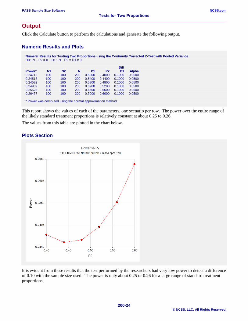
Numeric Results for Testing Two Proportions using the Continuity Corrected Z-Test with Pooled Variance H0: P1 - P2 = 0. H1: P1 - P2 = D1 ≠ 0. Diff Power* N1 N2 N P1 P2 D1 Alpha 0.24712 100 100 200 0.5000 0.4000 0.1000 0.0500 0.24518 100 100 200 0.5400 0.4400 0.1000 0.0500 0.24582 100 100 200 0.5800 0.4800 0.1000 0.0500 0.24909 100 100 200 0.6200 0.5200 0.1000 0.0500 0.25523 100 100 200 0.6600 0.5600 0.1000 0.0500 0.26477 100 100 200 0.7000 0.6000 0.1000 0.0500 * Power was computed using the normal approximation method.

This report shows the values of each of the parameters, one scenario per row. The power over the entire range of the likely standard treatment proportions is relatively constant at about 0.25 to 0.26. The values from this table are plotted in the chart below.

Plots Section

It is evident from these results that the test performed by the researchers had very low power to detect a difference of 0.10 with the sample size used. The power is only about 0.25 or 0.26 for a large range of standard treatment proportions.



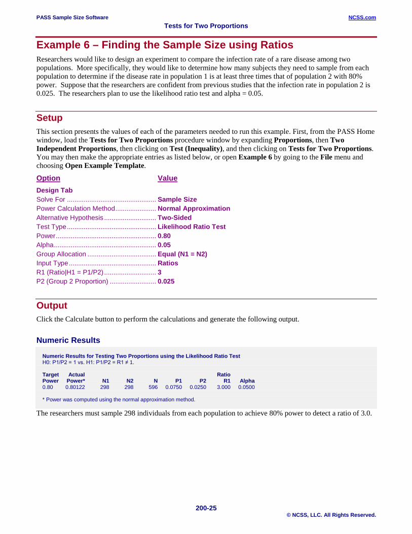
Example 6 – Finding the Sample Size using Ratios Researchers would like to design an experiment to compare the infection rate of a rare disease among two populations. More specifically, they would like to determine how many subjects they need to sample from each population to determine if the disease rate in population 1 is at least three times that of population 2 with 80% power. Suppose that the researchers are confident from previous studies that the infection rate in population 2 is 0.025. The researchers plan to use the likelihood ratio test and alpha = 0.05.


Option Value Design Tab Solve For ................................................ Sample Size Power Calculation Method ...................... Normal Approximation Alternative Hypothesis ............................ Two-Sided Test Type ................................................ Likelihood Ratio Test Power ...................................................... 0.80 Alpha ....................................................... 0.05 Group Allocation ..................................... Equal (N1 = N2) Input Type ............................................... Ratios R1 (Ratio|H1 = P1/P2) ............................ 3 P2 (Group 2 Proportion) ......................... 0.025


Numeric Results Numeric Results for Testing Two Proportions using the Likelihood Ratio Test H0: P1/P2 = 1 vs. H1: P1/P2 = R1 ≠ 1. Target Actual Ratio Power Power* N1 N2 N P1 P2 R1 Alpha 0.80 0.80122 298 298 596 0.0750 0.0250 3.000 0.0500 * Power was computed using the normal approximation method.

The researchers must sample 298 individuals from each population to achieve 80% power to detect a ratio of 3.0.



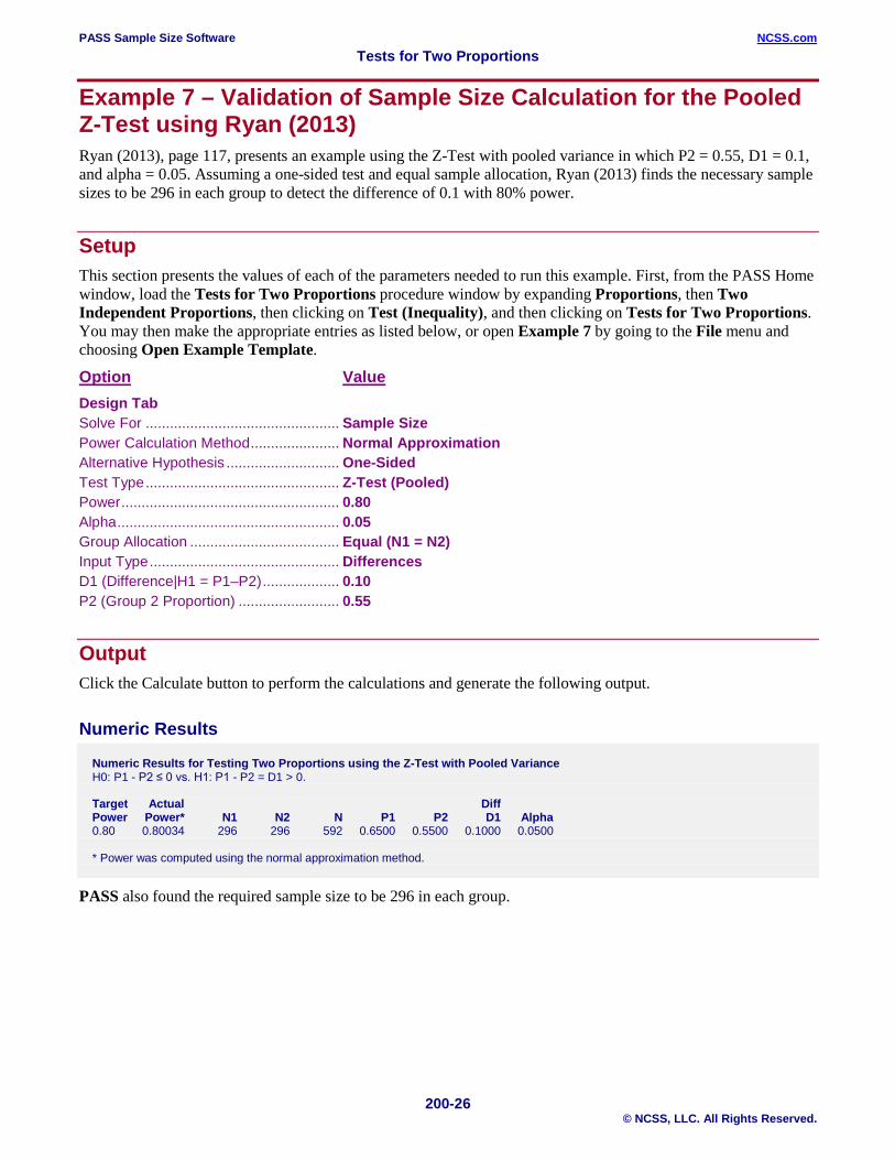
Example 7 – Validation of Sample Size Calculation for the Pooled Z-Test using Ryan (2013) Ryan (2013), page 117, presents an example using the Z-Test with pooled variance in which P2 = 0.55, D1 = 0.1, and alpha = 0.05. Assuming a one-sided test and equal sample allocation, Ryan (2013) finds the necessary sample sizes to be 296 in each group to detect the difference of 0.1 with 80% power.


Option Value Design Tab Solve For ................................................ Sample Size Power Calculation Method ...................... Normal Approximation Alternative Hypothesis ............................ One-Sided Test Type ................................................ Z-Test (Pooled) Power ...................................................... 0.80 Alpha ....................................................... 0.05 Group Allocation ..................................... Equal (N1 = N2) Input Type ............................................... Differences D1 (Difference|H1 = P1–P2) ................... 0.10 P2 (Group 2 Proportion) ......................... 0.55


Numeric Results Numeric Results for Testing Two Proportions using the Z-Test with Pooled Variance H0: P1 - P2 ≤ 0 vs. H1: P1 - P2 = D1 > 0. Target Actual Diff Power Power* N1 N2 N P1 P2 D1 Alpha 0.80 0.80034 296 296 592 0.6500 0.5500 0.1000 0.0500 * Power was computed using the normal approximation method.

PASS also found the required sample size to be 296 in each group.



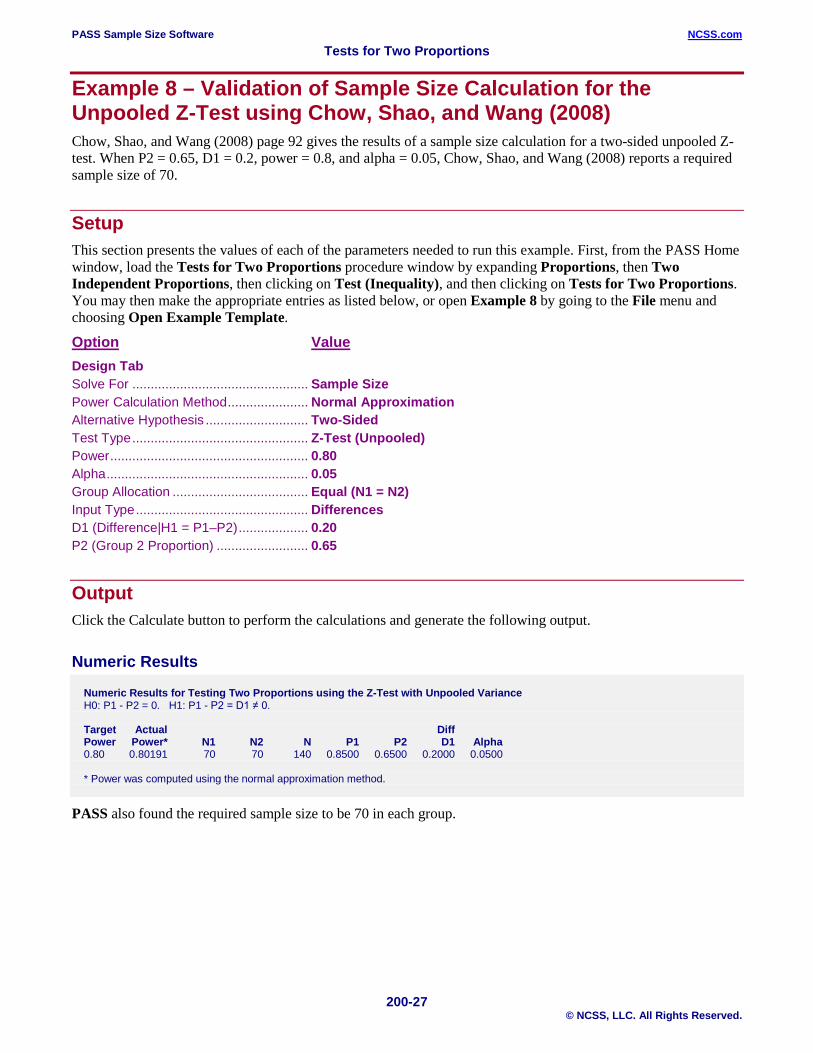
Example 8 – Validation of Sample Size Calculation for the Unpooled Z-Test using Chow, Shao, and Wang (2008) Chow, Shao, and Wang (2008) page 92 gives the results of a sample size calculation for a two-sided unpooled Z-test. When P2 = 0.65, D1 = 0.2, power = 0.8, and alpha = 0.05, Chow, Shao, and Wang (2008) reports a required sample size of 70.


Option Value Design Tab Solve For ................................................ Sample Size Power Calculation Method ...................... Normal Approximation Alternative Hypothesis ............................ Two-Sided Test Type ................................................ Z-Test (Unpooled) Power ...................................................... 0.80 Alpha ....................................................... 0.05 Group Allocation ..................................... Equal (N1 = N2) Input Type ............................................... Differences D1 (Difference|H1 = P1–P2) ................... 0.20 P2 (Group 2 Proportion) ......................... 0.65


Numeric Results Numeric Results for Testing Two Proportions using the Z-Test with Unpooled Variance H0: P1 - P2 = 0. H1: P1 - P2 = D1 ≠ 0. Target Actual Diff Power Power* N1 N2 N P1 P2 D1 Alpha 0.80 0.80191 70 70 140 0.8500 0.6500 0.2000 0.0500 * Power was computed using the normal approximation method.

PASS also found the required sample size to be 70 in each group.



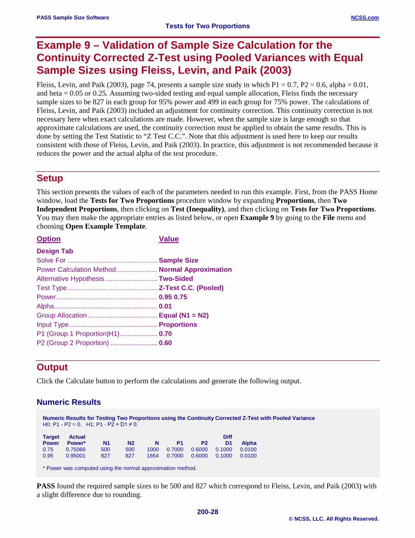
Example 9 – Validation of Sample Size Calculation for the Continuity Corrected Z-Test using Pooled Variances with Equal Sample Sizes using Fleiss, Levin, and Paik (2003) Fleiss, Levin, and Paik (2003), page 74, presents a sample size study in which P1 = 0.7, P2 = 0.6, alpha = 0.01, and beta = 0.05 or 0.25. Assuming two-sided testing and equal sample allocation, Fleiss finds the necessary sample sizes to be 827 in each group for 95% power and 499 in each group for 75% power. The calculations of Fleiss, Levin, and Paik (2003) included an adjustment for continuity correction. This continuity correction is not necessary here when exact calculations are made. However, when the sample size is large enough so that approximate calculations are used, the continuity correction must be applied to obtain the same results. This is done by setting the Test Statistic to “Z Test C.C.”. Note that this adjustment is used here to keep our results consistent with those of Fleiss, Levin, and Paik (2003). In practice, this adjustment is not recommended because it reduces the power and the actual alpha of the test procedure.


Option Value Design Tab Solve For ................................................ Sample Size Power Calculation Method ...................... Normal Approximation Alternative Hypothesis ............................ Two-Sided Test Type ................................................ Z-Test C.C. (Pooled) Power ...................................................... 0.95 0.75 Alpha ....................................................... 0.01 Group Allocation ..................................... Equal (N1 = N2) Input Type ............................................... Proportions P1 (Group 1 Proportion|H1) .................... 0.70 P2 (Group 2 Proportion) ......................... 0.60


Numeric Results Numeric Results for Testing Two Proportions using the Continuity Corrected Z-Test with Pooled Variance H0: P1 - P2 = 0. H1: P1 - P2 = D1 ≠ 0. Target Actual Diff Power Power* N1 N2 N P1 P2 D1 Alpha 0.75 0.75066 500 500 1000 0.7000 0.6000 0.1000 0.0100 0.95 0.95001 827 827 1654 0.7000 0.6000 0.1000 0.0100 * Power was computed using the normal approximation method.

PASS found the required sample sizes to be 500 and 827 which correspond to Fleiss, Levin, and Paik (2003) with a slight difference due to rounding.



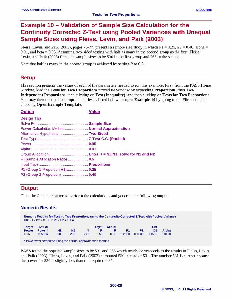
Example 10 – Validation of Sample Size Calculation for the Continuity Corrected Z-Test using Pooled Variances with Unequal Sample Sizes using Fleiss, Levin, and Paik (2003) Fleiss, Levin, and Paik (2003), pages 76-77, presents a sample size study in which P1 = 0.25, P2 = 0.40, alpha = 0.01, and beta = 0.05. Assuming two-sided testing with half as many in the second group as the first, Fleiss, Levin, and Paik (2003) finds the sample sizes to be 530 in the first group and 265 in the second.

Note that half as many in the second group is achieved by setting R to 0.5.


Option Value Design Tab Solve For ................................................ Sample Size Power Calculation Method ...................... Normal Approximation Alternative Hypothesis ............................ Two-Sided Test Type ................................................ Z-Test C.C. (Pooled) Power ...................................................... 0.95 Alpha ....................................................... 0.01 Group Allocation ..................................... Enter R = N2/N1, solve for N1 and N2 R (Sample Allocation Ratio) ................... 0.5 Input Type ............................................... Proportions P1 (Group 1 Proportion|H1) .................... 0.25 P2 (Group 2 Proportion) ......................... 0.40


Numeric Results

Numeric Results for Testing Two Proportions using the Continuity Corrected Z-Test with Pooled Variance H0: P1 - P2 = 0. H1: P1 - P2 = D1 ≠ 0. Target Actual Target Actual Diff Power Power* N1 N2 N R R P1 P2 D1 Alpha 0.95 0.95066 531 266 797 0.50 0.50 0.2500 0.4000 -0.1500 0.0100 * Power was computed using the normal approximation method.

PASS found the required sample sizes to be 531 and 266 which nearly corresponds to the results in Fleiss, Levin, and Paik (2003). Fleiss, Levin, and Paik (2003) computed 530 instead of 531. The number 531 is correct because the power for 530 is slightly less than the required 0.95.

tests for two proportions - ncss

Documents