tex class copernicus.cls. date: 4 november 2014 meteoio 2 ... filemanuscript prepared for geosci....

Discussion

Paper

|D

iscussionPaper

|D

iscussionPaper

|D

iscussionPaper

|

Manuscript prepared for Geosci. Model Dev. Discuss.with version 2014/07/29 7.12 Copernicus papers of the LATEX class copernicus.cls.Date: 4 November 2014

MeteoIO 2.4.2: a preprocessing library formeteorological dataM. Bavay1 and T. Egger2

1WSL Institute for Snow and Avalanche Research SLF, Flüelastrasse 11,7260 Davos Dorf, Switzerland2Egger Consulting, Postgasse 2, 1010 Vienna, Austria

Correspondence to: M. Bavay ([email protected])

1

Discussion

Paper

|D

iscussionPaper

|D

iscussionPaper

|D

iscussionPaper

|

Abstract

Using numerical models which require large meteorological data sets is sometimes difficultand problems can often be traced back to the Input/Output functionality. Complex modelsare usually developed by the environmental sciences community with a focus on the coremodelling issues. As a consequence, the I/O routines that are costly to properly implementare often error-prone, lacking flexibility and robustness. With the increasing use of suchmodels in operational applications, this situation ceases to be simply uncomfortable andbecomes a major issue.

The MeteoIO library has been designed for the specific needs of numerical models thatrequire meteorological data. The whole task of data preprocessing has been delegatedto this library, namely retrieving, filtering and resampling the data if necessary as well asproviding spatial interpolations and parametrizations. The focus has been to design an Ap-plication Programming Interface (API) that (i) provides a uniform interface to meteorologicaldata in the models; (ii) hides the complexity of the processing taking place; and (iii) guar-antees a robust behaviour in case of format errors, erroneous or missing data. Moreover,in an operational context, this error handling should avoid unnecessary interruptions in thesimulation process.

A strong emphasis has been put on simplicity and modularity in order to make it extremelyeasy to support new data formats or protocols and to allow contributors with diverse back-grounds to participate. This library can also be used in the context of High PerformanceComputing in a parallel environment

:is

:::::also

:::::::::regularly

:::::::::::evaluated

:::for

:::::::::::computing

::::::::::::::performance

::::and

:::::::further

::::::::::optimized

:::::::where

:::::::::::necessary. Finally, it is released under an Open Source license

and is available at http://models.slf.ch/p/meteoio.This paper gives an overview of the MeteoIO library from the point of view of conceptual

design, architecture, features and computational performance. A scientific evaluation of theproduced results is not given here since the scientific algorithms that are used have alreadybeen published elsewhere.

2

http://models.slf.ch/p/meteoio

Discussion

Paper

|D

iscussionPaper

|D

iscussionPaper

|D

iscussionPaper

|

1 Introduction

1.1 Background

Users of numerical models for environmental sciences must handle the meteorological forc-ing data with care, since they have a very direct impact on the simulation’s results. Theforcing data come from a wide variety of sources, such as files following a specific format,databases hosting data from meteorological networks or web services distributing data sets.A significant time investment is necessary to retrieve the data, look for potentially invaliddata points and filter them out, sometimes correcting the data for various effects and finallyconverting them to a format and units that the numerical model supports. These steps areboth time intensive and error prone and usually cumbersome for new users (similarly towhat has been observed for Machine Learning, Kotsiantis et al., 2006).

From the point of view of the model developer, handling input data is usually a necessarybut unpleasant side of model development that distracts from working on the core featuresof the model. As a consequence developers tend to spend minimal effort on these aspects.Throughout the history of the model, more pre-processing routines will usually be added tothe code in order to handle data-related problems as they arise. Moreover, supporting newdata formats and/or protocols for specific projects, requires modifying the code by eitheradding conditional compilation directives or tweaking the current routines. This means thatthe data reading and preprocessing routines will often be of low quality, lacking robustnessand efficiency as well as flexibility, exacerbating the troubles met by the users in preparingtheir data for the model.

::A

:::::few

:::::::::libraries

:::or

::::::::::software

:::::::::already

:::::::tackle

:::::::these

::::::::issues,

::::for

::::::::::example

::::the

:::::::::::SAFRAN

:::::::::::::preprocessor

:::of

:::the

:::::::::::CROCUS

:::::snow

:::::::model

:(Durand et al., 1993)

:,:::the

::::::::::PREVAH

::::::::::::::preprocessor

::of

::::the

:::::::::PREVAH

:::::::::::::hydrological

:::::::model

:(Viviroli et al., 2009)

::or

::::the

::::::::::MicroMet

:::::::model (Liston and

Elder, 2006):.:::::::::However

:::::::these

::::::::projects

::::are

::::::often

:::::very

::::::tightly

:::::::linked

::::with

::a::::::::specific

:::::::model

:::::and

:::::::::::::infrastructure

:::::and

::::are

::::::::typically

::::not

:::::able

:::to

::::::::operate

::::::::outside

::::this

:::::::::specific

::::::::context.

::::::They

::::::often

::::lack

:::::::::flexibility

:::for

:::::::::example

::::::::::requiring

:::::their

::::::users

:::to

::::::::convert

:::::their

:::::data

::to

::a::::::::specific

::::file

::::::::format,

::by

::::::hard

:::::::coding

::::the

::::::::::::processing

::::::steps

:::for

::::::each

:::::::::::::::meteorological

::::::::::::parameter

::or

:::by

::::::::::requiring

:::to

3

Discussion

Paper

|D

iscussionPaper

|D

iscussionPaper

|D

iscussionPaper

|

:::be

:::run

:::::::::through

:a:::::::::specific

::::::::::interactive

::::::::::interface.

::::::They

::::also

::::::often

::::rely

:::on

::a::::::::specific

::::::input

:::::::and/or

::::::output

::::::::::sampling

:::::rate

::::and

:::::can

:::not

:::::deal

:::::with

:::::fully

:::::::::arbitrary

::::::::::sampling

::::::rates.

::::::::::MeteoIO

:::::aims

:::to

::::::::::overcome

::::::these

:::::::::::limitations

::::and

:::to

:::be

::a

::::::::general

:::::::::purpose

::::::::::::::preprocessor

::::that

:::::::::different

::::::::models

::::can

::::::easily

::::::::::integrate.

:

1.2 Data quality

A most important aspect of data preprocessing is the filtering of data based on their per-ceived quality. The aim of filtering data is to remove the mismatch between the view of thereal-world system that can be inferred from the data and the view that can be obtained bydirectly observing the real-world system (Wand and Wang, 1996). We focus on two dataquality dimensions: accuracy and consistency.

We define accuracy as “the recorded value is in conformity with the actual value” (Ballouand Pazer, 1985). Inaccuracies occur because of a sensor failure (the sensor itself fails tooperate properly), because of the conditions of the immediate surroundings of the sensor(the sensor conditions do not reflect the local conditions, such as a frozen anemometer) orbecause of physical limitations of the sensor (such as precipitation undercatch).

We define consistency in a physical sense, that a data set should obey the physical lawsof nature. Practically, the time evolution of a physical parameter as well as the interactionsbetween different physical parameters must obey the laws of nature.

1.3 Design goals

In order to help the users of numerical models consuming meteorological data and reducetheir need for support, we developed new meteorological data reading routines and investedsignificant efforts in improving the overall usability by working on several dimensions of theergonomic criteria (Scapin and Bastien, 1997), adapting them according to the needs ofa data preprocessing library:

– Guidance: providing a clear structure to the user:;:

– Grouping/distinction of items: so the user sees which items are related;:

4

Discussion

Paper

|D

iscussionPaper

|D

iscussionPaper

|D

iscussionPaper

|

– Consistency: adapt and follow some rules regarding the naming, syntax and han-dling of input parameters

:;

– Workload: focusing on the tasks that the user wants to accomplish:;:

– Minimal actions: limit as much as possible the number of steps for each tasks:;:

– Explicit control: let the user explicitly define the tasks that have to be performed:;

– Error management: helping the user detect and recover from errors:;:

– Error protection: handle all possible user input errors;:

– Quality of error messages: provide clear and relevant error messages.:

We also identified two distinct usage scenarios:Research usage. The end user runs the model multiple times on the same data, with

some highly tuned parameters in order to produce a simulation for a paper or project. Theemphasis is put on flexibility and configurability (Scapin and Bastien, 1997).

Operational usage. The model is run fully or partially unattended for producing regularoutputs. Once configured, the simulations’ setup remains the same for an extended periodof time. The emphasis is put on robustness and stability.

We decided to tackle both scenarios with the same software package and ended up withthe following goals:

– Isolate the data reading routines from the rest of the model;

– Implement robust data handling with relevant error messages for the end user;

– Allow the data model to be easily expanded (data model scalability);:

– Make it possible to easily change the data source (format and/or protocol) without anychange in the model code itself;

– Preprocess the data on the fly;5

Discussion

Paper

|D

iscussionPaper

|D

iscussionPaper

|D

iscussionPaper

|

– Implement a “best effort” approach with reasonable fallback strategies in order to in-terrupt the simulation process only in the most severe cases;

– Let the end user configure the whole data reading and preprocessing in a configura-tion file that can be saved for archiving or later use.

2 Architecture

Using the design philosophy guidelines laid out in Sect. 1.3 and in order to be able to reusethis software package in other models, we decided to implement this software packageas a library named MeteoIO. We chose the C++ language in order to benefit from theobject oriented model as well as good performance and relatively easy interfacing with otherprogramming languages. We also decided to invest a significant effort in documenting thesoftware package both for the end users and for developers who would like to integrate itinto their own models. More architectural principles are laid out in the sections below whilethe implementation details are given in Sects. 3 and 4.

2.1 Actors

The question of proper role assignment (Yu and Mylopoulos, 1994), or finding out whoshould decide, is central to the development of MeteoIO: carefully choosing if the end user,the model relying on MeteoIO or MeteoIO itself is the appropriate actor to take a specificdecision has been a recurring question in the general design. For example when temporallyresampling data, the method should be chosen by the end user while the sampling rate isgiven by the numerical model and the implementation details and error handling belong toMeteoIO.

2.2 Dependencies

When complex software packages grow, they often require more and more external depen-dencies (as third party software libraries or third party tools). When new features are added,

6

Discussion

Paper

|D

iscussionPaper

|D

iscussionPaper

|D

iscussionPaper

|

it is natural to try to build on achievements of the community and not “reinvent the wheel”.However this also has some drawbacks:

– these third party components must be present on the end user’s computer;

– these components need to be properly located when compiling or installing the soft-ware package;

– these components have their own evolution, release schedule and platform support.

Therefore, as relying more on external components reduces the core development effort,it significantly increases the integration effort. One must then carefully balance these twocosts and choose the solution that will yield the least long term effort.

Estimating that a complex integration issue represents a few days of work and a nonnegligible maintenance effort, core MeteoIO features that were feasible to implement withina few days were redeveloped instead of integrating existing solutions. For the more periph-eral features (like output plug-ins) we decided to rely on the most basic libraries at hand,disregarding convenient wrappers which would introduce yet another dependency, and togive the user the possibility to decide which features to enable at compile time. Accordingly,MeteoIO requires no dependencies by default when it would have required more than fifteenif no such mitigation strategy had been taken. A handful of dependencies can be activatedwhen enabling all the optional features.

2.3 Manager/worker architecture

Many tasks have been implemented as a manager/worker architecture: a manager offersa high level interface to the task (filtering, temporal interpolation, . . . ) while a worker imple-ments the low level, MeteoIO-agnostic core processing. The manager class implements thenecessary features to efficiently convert MeteoIO-centric concepts and objects to generic,low level data ideal for processing. All of the heavily specialized programming concepts (ob-ject factories, method pointers, etc) and their actual implementations are therefore hiddenfrom both the high level calls and the low level processing. This architecture balances the

7

Discussion

Paper

|D

iscussionPaper

|D

iscussionPaper

|D

iscussionPaper

|

needs of the casual developer using the library (relying on very simple, high level calls) aswell as the casual developer expanding the library by contributing some core processingmodules (data sources, data filters, etc).

Although this approach might seem inefficient (by adding extra steps in the data pro-cessing), it has contributed to the performance gains (as shown in Sect. 5.2) by making itpossible to rely on standard, optimized routines.

2.4 Flexibility

Since we don’t not want the user to have to recompile either MeteoIO or:::::::::::::Hard-coding

::::the

::::data

::::::::::::::::preprocessing

::in:::::

the:::::::source

::::::code

:::is

:::an

::::::easy

:::::::::::possibility

::::but

:::::::::requires

:::::that

::::the

::::::user

:::::::::::recompiles

:his model when configuring the data preprocessing, everything has to be done

dynamically. All:.:::In

::::::order

::to

::::::avoid

::::this

:::::and

:::::thus

:::::offer

::::::more

::::::::::flexibility,

:::all adjustable param-

eters are configured in a::::text

:file following the more or less standard INI ASCII format.

This makes it possible to manually configure the preprocessing , copy elements:::::::simply

::by

::::::::editing

::a:::::text

::::file,

:::::::::copying

:::::::::::::configuration

::::::::::sections

:between different simulations , keep

the whole configuration description with the simulation results and potentially provide::::and

::::::::::potentially

::::::::::providing

:a graphical user interface to help the user configure his simulation

(Bavay and Egger, 2014).::::::::::Moreover,

::::::::instead

:::of

:::::::having

:::to

::::::keep

::::::::multiple

:::::files

::::::::::::::representing

:::the

::::::data

::at

:::::::::various

:::::::::::::intermediate


::::::stage

:::::::::::alongside

::a::::::::

textual::::::::::::description

:::of

::::the

:::::::::::processing

::::::steps

::::that

::::::have

::::::been

::::::::applied,

::it::is

:::::::::possible

:::to

:::::only

:::::::archive

::::the

::::raw

:::::data

:::::and

::::the

:::::::::::::configuration

::::file

::::that

:::::then

:::::acts

:::as

::a

:::::::::::::::representation

::of

::::the

:::::::::::::::preprocessing

::::::::::workflow.

:

For clarity, each step of the data reading, preprocessing and writing is described in its ownsection in the configuration file. There is no central repository or validation of the keys to befound in this file, leaving each processing component free to manage its own configurationkeys. On the other hand there is no global overview of which keys might have been providedby the user but will not be used by any component.

No assumptions are made about the sampling rate of the data read or the data requiredby the caller. It is assumed that the input data can be sampled at any rate, including irregularsampling and can be resampled to any timestamp, as requested by the caller. Moreover

8

Discussion

Paper

|D

iscussionPaper

|D

iscussionPaper

|D

iscussionPaper

|

any data field can be nodata at any time. This means that a given data set might containfor example precipitation sampled once a day, temperatures sampled twice an hour andsnow height irregularly sampled. Practically, this prevents us from using standard signalprocessing algorithms for resampling data, because these commonly assume a constantsampling rate and require that all timestamps have a value.

2.5 Modularity

A key to the long term success of a software package is the modularity of its internal com-ponents. The choice of an object oriented language (C++) has helped tremendously to buildmodular elements that are then combined to complete the task. The data storage classesare built on top of one another (through inheritance or by integrating one class as a mem-ber of another one) while the data path management is mostly built as a manager that linksall the necessary components. A strong emphasis has been put on encapsulation by an-swering, for each new class, the following question: How should the caller interact with thisobject in an ideal world? Then the necessary implementation has been developed from thispoint of view, adding “non-ideal” bindings only when necessary for practical reasons.

2.6 Promoting interdisciplinary contributions

Modularity, by striving to define each data processing in a very generic way and by makingeach one independent of the others, presents external contributors with a far less intimi-dating context to contribute. The manager/worker approach shown in Sect. 2.3 also facil-itates keeping the modules that are good candidates for third party contributions simpleand generic. Some templates providing a skeleton of what should be implemented are alsoprovided alongside documentation on how to practically contribute with a short list of pointsto follow for each kind of contribution (data plug-in, processing element, temporal or spatialinterpolation).

9

Discussion

Paper

|D

iscussionPaper

|D

iscussionPaper

|D

iscussionPaper

|

2.7 Coding standards and methodology

The project started in late 2008 and is currently comprised of more than 52 000 lines, con-tributed by twelve contributors. 95 % of the code originates from the two main contributors.The code mostly follows the kernel coding style as well as the recommendations given by(Rouson et al., 2011), giving the priority to code clarity. Literate programming is used withthe doxygen tool (van Heesch, 2008).

Coding quality is enforced by requesting all committed code to pass the most stringentcompiler warnings (all possible warnings on gcc) including the compliance checks with rec-ommended best practices for C++ (Meyers, 1992). The code currently compiles on Linux,Windows, OS X and Android.

The development methodology is mostly based on Extreme Programming (Beck andAndres, 2004) with short development cycles of limited scope, architectural flexibility andevolutions, frequent code reviews and daily integration testing. The daily integration testinghas been implemented with ctest (Martin and Hoffman, 2007), validating the core featuresof MeteoIO and recording the run time for each test. This shows performance regressionsalongside feature regressions. Regular static analysis is performed using Cppcheck (Mar-jamäki, 2013) and less regularly with Flawfinder (Wheeler, 2013) to detect potential securityflaws. Regular leak checks and profiling is performed relying on the Valgrind instrumentationframework (Seward et al., 2013; Nethercote and Seward, 2007).

The code has also been adapted to interact easily with several parallelizationtechnologies as well as optimized to benefit from single instruction, multiple data (SIMD)capabilities when feasible . The necessary serialization methods have been implementedfor the POPC extension to C++ as well as for the Message Passing Interface (MPI). For thelatter,

::::and

:some kind of a universal serialization has been implemented

::to

::::::ease

::::the

::::use

:::of

:::::::::MeteoIO

:::::::objects

:::::::within

::a

:::::::parallel

::::::::::::application: each storage class implements the redirection

operators, serializing and deserializing to/from a standard iostream object. This object isthen passed to MPI

:::the

:::::::::::::::parallelization

::::::toolkit

:::or

:::::::library

::::::(such

:::as

:::::MPI,

::::the

::::::::::Message

:::::::::Passing

::::::::::Interface) as a pure C structure through a very simple wrapper in the calling application.

10

Discussion

Paper

|D

iscussionPaper

|D

iscussionPaper

|D

iscussionPaper

|

3 Data structures

All data classes rely on the Standard Template Library (STL) (Musser et al., 2001) to a largeextent that is available on all C++ compilers and may provide some low level optimizationswhile being quite high level. The design of the STL is also consistent and therefore a goodmodel to follow: the data classes in MeteoIO follow the naming scheme and logic of theSTL whereever possible, making them easier to use and remember by a developer whohas some experience with the STL. They have been designed around the following specificrequirements:

– Offer high level features for handling meteorological data and related data. Using themshould make the calling code simpler.

– Implement a standard and consistent interface. Their interface must be obvious to thecaller.

– Implement them in a robust and efficient way. Using them should make the callingcode more robust and faster.

The range of high level features has been defined according to the needs of models rely-ing on MeteoIO as well as in terms of completeness. When appropriate and unambiguousthe arithmetic operators and comparison operators have been implemented. Each internaldesign decision has been based on careful benchmarking.

Great care has been taken to ensure that the implemented functionality behaves as ex-pected. Of specific concern is that corner cases (or even plain invalid calls) should neverproduce a wrong result but strive to produce the expected result or return an exception.A silent failure would lead to possibly erroneous results in the user application and musttherefore be avoided at all cost.

3.1 Configuration

In order to automate the process of reading parameters from the end user configurationfile, a specific class has been created to manage configuration parameters. The Config

11

Discussion

Paper

|D

iscussionPaper

|D

iscussionPaper

|D

iscussionPaper

|

class stores the configuration options as a key-value couple of strings in a map. The key isbuilt by prefixing the actual key with the section it belongs to. When calling a getter to reada parameter from the Config object, it converts data types on the fly through templates.It also offers several convenience methods, such as the possibility of requesting all keysmatching a (simple) pattern or all values whose keys match a (simple) pattern.

3.2 Dates

The Date class stores the GMT Julian day (including the time) alongside the timezoneinformation (because leap seconds are not supported, the reference is defined as beingGMT instead of UTC). The Julian day is stored in double precision which is enough for onesecond resolution while keeping dates arithmetic and comparison operators efficient. Theconversion to and from split values is done according to (Fliegel and van Flandern, 1968).The conversion to and from various other time representations as well as various formattedtime strings and rounding is implemented.

3.3 Geographic coordinates

The geographic coordinates are converted and stored as latitude, longitude and altitude inWGS84 by the Coords class. This allows an easy conversion to and from various Cartesiangeographic coordinates systems with a moderate loss of precision (on the order of onemeter) that is still compatible with their use for meteorological data. Two different strategieshave been implemented for dealing with the coordinate conversions:

– Relying on a the proj4 third party library (pro, 2013). This enables to support all coor-dinate systems but brings an external dependency.

– Implementing the conversion to and from latitude/longitude. This does not bring anyexternal dependency but requires some specific (although usually limited) develop-ment.

12

Discussion

Paper

|D

iscussionPaper

|D

iscussionPaper

|D

iscussionPaper

|

Therefore the coordinate systems that are most commonly used by MeteoIO’s users havebeen reimplemented (currently the Swiss CH1903 coordinates, UTM and UPS Hager et al.,1989) and seldom used coordinate systems are supported by the third party library. It isalso possible to define a local coordinate system that uses a reference point as origin andcomputes easting and northing from this point using either the law of cosine or the Vincentyalgorithm (Vincenty, 1977) for distance calculations. These algorithms are also part of theAPI and thus available to the developer.

3.4 Meteorological data sets

The meteorological data are centered around the concept of a weather station: one ormore meteorological parameters (in the MeteoData class) measured at one location (thislocation can change in time). The station has coordinates (including an elevation) and oftena name or identifier associated with it as well as a slope and azimuth (all belonging to theStationData class). For each timestamp, a predefined set of meteorological parameters hasbeen defined and parameters that are not available receive a nodata value. This set canbe extended by defining additional parameters that will then be handled the same way asthe fixed parameters. Some basic merging strategies have been implemented in order tomerge measurements from close stations (for example when a set of instruments belongs toa given measuring network and another set, installed on the same mast belongs to anothernetwork).

A static map does the mapping between predefined meteorological parameters (definedas an enum) and an index. A vector of strings stores a similar mapping between the pre-defined meteorological parameters’ names as strings and the same index (i.e. a vector ofnames). Finally a vector of doubles (data vector) stores the actual data for each meteoro-logical parameter, according to the index defined in the static map or names vector. Whenan extra parameter is added, an new entry is created in the names vector as well as a newentry in the data vector at the same index. The total number of defined meteorological pa-rameters is updated, making it possible to access a given meteorological field either byindex (looping between zero and the total number of fields), by name (as string) or by pre-

13

Discussion

Paper

|D

iscussionPaper

|D

iscussionPaper

|D

iscussionPaper

|

defined name (as enum). Methods to retrieve an index from a string or a string from anindex (or enum) are also available.

3.5 Grids

Grids have been implemented for one dimensional to four dimensional data as templatesin the Array classes in order to accommodate different data types. They are based on thestandard vector container and define the appropriate access by index (currently as row ma-jor order) as well as several helper methods (retrieving the minimum, maximum or meanvalue of the data contained in the grid, for example) and standard arithmetic operators be-tween grids and between a grid and a scalar. A geolocalized version has been implementedin the GridObject classes that brings about added safety in the calling code by making itpossible to check that two grids refer to the same domain before using them.

3.6 Digital elevation model

A special type of two dimensional grid (based on the Grid2DObject class) has been de-signed to contain digital elevation model (DEM) data. This DEMObject class automaticallycomputes the slope, azimuth and curvature as well as the surface normal vectors. It lets thedeveloper choose between different algorithms: maximum downhill slope (Dunn and Hickey,1998), four neighbours algorithm (Fleming and Hoffer, 1979) or two triangle method (Cor-ripio, 2003) with an eight-neighbour algorithm for border cells (Horn, 1981). The azimuthis always computed using (Hodgson, 1998). The two triangle method has been rewrittenin order to be centered on the actual cell instead of node-centered, thus working with a lo-cal 3× 3 grid centered around the pixel of interest instead of 2× 2. The normals are alsocomputed as well as the curvatures, using the method of (Liston and Elder, 2006).

The evaluation of the local slope relies on the eight immediate neighbours of the currentcell. Because this offers only a limited number of meaningful combinations for computingthe slope, some more recent slope calculation algorithms that have been explored are ac-tually exactly equivalent to the previously listed algorithms. In order to transparently handle

14

Discussion

Paper

|D

iscussionPaper

|D

iscussionPaper

|D

iscussionPaper

|

the special cases represented by the borders (including cells bordering holes in the digitalelevation model), a 3×3 grid is filled with the content of the cells surrounding the current cell.Cells that cannot be accessed (because they don’t exist in the DEM) are replaced by nodatavalues. Then each slope algorithm works on this subgrid and implements workarounds ifsome required cells are set to nodata in order to be able to provide a value for each pixelthat it received. This makes the handling of special cases very generic and computationallyefficient.

Various useful methods for working with a DEM are also implemented, for example thepossibility to compute the horizon of a grid cell or the terrain following distance between twopoints.

4 Components

4.1 Data flow overview

At the core of MeteoIO lies the process of getting for a specific time step either a set ofmeteorological data or a set of spatially interpolated meteorological data. The model usingMeteoIO for getting its meteorological time series relies on the very simple call given inlisting 1. This call returns a vector containing all the meteorological data that could beprovided at the requested date, grouped by stations with their metadata. Each parametereither contains nodata or the preprocessed value following the configuration by the enduser.

A model requiring spatially interpolated values will use the call shown in listing 2. This callreturns a grid filled with the spatially interpolated parameter as specified by meteoparam atthe requested date over the provided DEM. If the grid could not be filled according to therequirements provided by the user, the grid will be empty and the call will return false.

In the background, within MeteoIO, the process of providing the forcing data to the nu-merical model according to the constraints specified by the user has been split into severalsteps (see Fig. 4):

15

Discussion

Paper

|D

iscussionPaper

|D

iscussionPaper

|D

iscussionPaper

|

1. getting the raw data;

2. filtering and correcting the data;

3. temporally interpolating (or resampling) the data if necessary;

4. generating data from parametrizations if everything else failed;

5. spatially interpolating the data if requested.

Practically, the raw data is read by the IOHandler component through a system of plug-ins. These plug-ins are low level implementations providing access to specific data sourcesand can easily be developed by a casual developer. The data is read in bulk, between twotimestamps as defined by the BufferedIOHandler that implements a raw data buffer in orderto prevent having to read data out of the data source for the next caller’s query. This bufferis then given for filtering and resampling to the MeteoProcessor. This will first filter (andcorrect) the whole buffer (by passing it to the ProcessingStack ) since benchmarks haveshown that processing the whole buffer at once is less costly than processing individuallyeach time steps as they are requested. The MeteoProcessor then temporally interpolatesthe data to the requested time step (if necessary) by calling the Meteo1DInterpolator. A lastresort stage is provided by the DataGenerator that attempts to generate the potentiallymissing data (if the data could not be temporally interpolated) using parametrizations.

Finally, the data is either returned as such or spatially interpolated using the Me-teo2DInterpolator. The whole process is transparently managed by the IOManager thatremains the visible side of the library for requesting meteorological data. The IOManageroffers a high level interface as well as some configuration options, allowing for example toskip some of the processing stages. The caller can nevertheless decide to manually callsome of these components since they expose a developer-friendly, high level API.

4.2 Data reading

All the necessary adaptations for reading data from a specific data source are handledby a specifically construed plug-in for the respective data source. The interface exposed

16

Discussion

Paper

|D

iscussionPaper

|D

iscussionPaper

|D

iscussionPaper

|

by the plug-ins is very simple and their tasks very focused: they must be able to readthe data for a specific time interval or a specific parameter (for gridded data) and fill theMeteoIO data structures, converting the units to International System of Units (SI). Similarly,they must be able to receive some MeteoIO data structures and write them out. Severalhelper functions and classes are available to simplify the process. This makes it possiblefor a casual developer to readily develop his own plug-in, supporting his own data source,with very little overhead.

In its current version MeteoIO includes plug-ins for reading and/or writing time seriesand/or grids from Oracle and PostgreSQL databases, the Global Sensor Network (GSN)REST API (Michel et al., 2009), Cosmo XML (cos, 2013), GRIB, NetCDF, ARC ASCII,ARPS, GRASS, PGM, PNG, GEOtop, Snowpack and Alpine3D native file formats and a fewothers.

The proper plug-in for the user-configured data source is instantiated by the IOHandlerthat handles raw data reading. Usually, the IOHandler is itself called by the BufferedIOHan-dler in order to buffer the data for subsequent reads. The BufferedIOHandler is most oftencalled with a single timestamp argument, computes an appropriate time interval and callsIOHandler with this time interval, filling its internal buffer.

4.3 Data processing

IOManager utilises the methods exposed by the MeteoProcessor. This is a high level inter-face that transparently encloses both the data processing and the resampling stages. Thesetwo stages are handled by the ProcessingStack and the Meteo1DInterpolator, respectively.

The ProcessingStack reads the user configured filters and processing elements andbuilds a stack of ProcessingBlock objects for each meteorological parameter and in theorder declared by the end user. The time series are then passed to each individual Pro-cessingBlock, each block being one specific filter or processing implementation. These havebeen divided into three categories:

– processing elements;

17

Discussion

Paper

|D

iscussionPaper

|D

iscussionPaper

|D

iscussionPaper

|

– filters;

– filters with windowing.

The last two categories stem purely from implementation considerations: filtering a datapoint based on a whole data window yields different requirements than filtering a data pointindependently of the data series. Filters represent a form of processing where data pointsare either kept or rejected. The processing elements on the other hand alter the value ofone or more data points. Filters are used to detect and reject invalid data while processingelements are used to correct the data (for instance, correcting a precipitation input for un-dercatch or a temperature sensor for a lack of ventilation). These processing elements canalso be used for sensitivity studies, by adding an offset or multiplying by a given factor.

As shown in Fig. 6, each meteorological parameter is associated with a ProcessingStackobject that contains a vector of ProcessingElement objects (generated through an objectfactory). Each ProcessingElement object implements a specific data processing algorithm.The meteorological parameters mapping to their ProcessingStack is done in a standardmap object.

4.3.1 Filters

Filters are used to detect and reject invalid data and therefore either keep or reject datapoints but don’t modify their value. Often an optional keyword “soft” has been defined thatgives some flexibility to the filter. The following filters have been implemented:

min, max, min_max. These filters reject out of range values or reset them to the closestbound if “soft” is defined;

rate. This filters out data points if the rate of change is larger than a given value. Botha positive and a negative rate of change can be defined, for example for a different snowaccumulation and snow ablation rate;

standard deviation. All values outside of y± 3σ are removed;median absolute deviation. All values outside y± 3σMAD are removed;Tukey. Spike detection following (Goring and Nikora, 2002);

18

Discussion

Paper

|D

iscussionPaper

|D

iscussionPaper

|D

iscussionPaper

|

unheated rain gauge. This removes precipitation inputs that don’t seem physical. Thecriteria that is used is that for precipitation to really occur, the air and surface temperaturesmust be at most three degrees apart and relative humidity must be greater than 50 %. Thisfilter is used to remove invalid measurements from snow melting in an unheated rain gaugeafter a snow storm.

4.3.2 Processing elements

Processing elements represent processing that alters the value of one or more data points,usually to correct the data. The following processing elements have been implemented:

mean, median or wind average. Averages over a user-specified period. The period isdefined as a minimum duration and a minimum number of points. The window centeringcan be specified, either left, center or right. The wind averaging performs the averaging onthe wind vector;

Exponential or Weighted Moving Average. Smooths the data either with an Exponentialor Weighted Moving Average (EMA, WMA respectively) smoothing algorithm;

2 poles, low pass Butterworth. Low pass filter according to (Butterworth, 1930);add, mult, suppr. This makes it possible to add an offset or multiply by a given factor

:::::::::(constant

:::or

:::::::either

:::::::hourly,

:::::daily

:::or

:::::::::monthly

::::and

::::::::::provided

::in

::a:::::file), for sensitivity studies or

:::::::climate

::::::::change

:::::::::::scenarios

::or

:totally delete a given meteorological parameter;

unventillated temperature sensor correction. Corrects a temperature measurement forthe radiative heating on an unventilated sensor, according to (Nakamura and Mahrt, 2005)or (Huwald et al., 2009);

undercatch. Several corrections are offered for precipitation undercatch, either following(Hamon, 1972; Førland and Institutt, 1996) or following the WMO corrections (Goodisonet al., 1997). Overall, the correction coefficients for fifteen different rain gauges have beenimplemented. Since the WMO corrections were not available for shielded Hellmann raingauges, a fit has been computed based on published data (Wagner, 2009; Daqing et al.,1999). The correction for the Japanese RT-3 rain gauges has been implemented following

19

Discussion

Paper

|D

iscussionPaper

|D

iscussionPaper

|D

iscussionPaper

|

Yokoyama et al. (2003). It is also possible to specify fixed correction coefficients for snowand mixed precipitation;

precipitation distribution. The precipitation sum can be distributed over precedingtimesteps. This is useful for example when daily sums of precipitation are written at theend of the day in an otherwise hourly data set.

The data window can also be configured by the end user: by default the data is centeredaround the requested data point. But it is also possible to force the data window to be leftor right centered. An extra option “soft” allows the data window to be centered as specifiedby the end user if applicable or to shift the window according to a “best effort” strategy if thedata don’t permit the requested centering.

4.4 Resampling

If the timestamp requested by the caller is not present in the data (either it has been filteredout or it was not present from the beginning), temporal interpolations will be performed. TheMeteo1DInterpolator is responsible for calling a temporal interpolation method for each me-teorological parameter as configured by the end user. The end user chooses between thefollowing methods of temporal interpolation for each meteorological parameter separately:

no interpolation. If data exists for the requested timestamp it will be returned or remainnodata otherwise;

nearest neighbour. The closest data point in the raw data that is not nodata is returned;linear. The value is linearly interpolated between the two closest data points;accumulation. The raw data is accumulated over the period provided as argument;daily solar sum. The potential solar radiation is generated as to match the daily sum as

provided in the input data.These methods must be able to both downsample and upsample according to the needs

(except the daily solar sum). These methods take a time series as argument and a times-tamp and return the interpolated value for a given meteorological parameter. The ability tosupport an arbitrary and variable sampling rate for both the input and output data preventsthe utilisation of well known signal analysis algorithms. Moreover some meteorological pa-

20

Discussion

Paper

|D

iscussionPaper

|D

iscussionPaper

|D

iscussionPaper

|

rameters require a specific processing, such as precipitation that must be accumulated overa given period. The following approach has therefore been implemented (see in Fig. 7): foreach requested data point, if the exact timestamp cannot be found or in case of reaccumula-tion, the index where the new point should be inserted will be sought first. Then the previousvalid point is sought within a user-configured search distance. The next valid point is thensought within the user-configured search distance from the first point. Then the resamplingstrategy (nearest neighbour, linear or reaccumulation) uses these points to generate theresampled value. Other resampling algorithms may be implemented by the user that woulduse more data points.

When no previous or next point can be found, the resampling extrapolates the requestedvalue by looking at more valid data points respectively before or after the previously foundvalid points. Because of the significantly increased risk of generating a grossly out of boundvalue, this behaviour must be explicitly enabled by the end user.

4.5 Data generators

In order to be able to return a value for a given timestamp there must be enough dataavailable in the original data source. This data has to pass the filters set up by the end userand may then be used for resampling. In case that data is absent or filtered out there isstill a stage of last resort: the data can be generated by a parametrization relying on otherparameters. The end user configures a list of algorithms for each meteorological parameter.These algorithms are implemented as classes inheriting from the GeneratorAlgorithms. TheDataGenerator class acts as their high level interface. The algorithms range from very basic,such as assigning a constant value, to quite elaborate. For instance the measured incomingsolar radiation is compared to the potential solar radiation resulting in a solar index. Thesolar index is used in a parametrization to compute a cloud cover that is given to anotherparametrization to compute a long wave radiation.

The GeneratorAlgorithms receive a set of meteorological parameters for one point andone timestamp. The DataGenerator walks through the user configured list of generators,in the order of their declaration by the end user, until a valid value can be returned. The

21

Discussion

Paper

|D

iscussionPaper

|D

iscussionPaper

|D

iscussionPaper

|

returned value is inserted into the data set and either returned to the caller or used forspatial interpolations.

The following generators have been implemented:standard pressure. Generates a standard pressure that only depends on the elevation;constant. Generates a constant value as provided by the user;sinusoidal. Generates a value with sinusoidal variation, either on a daily or a yearly pe-

riod. The minimum and maximum values are given as arguments as well as the position ofthe first minimum;

clearsky:::::::relative

::::::::::humidity.

:::::::::::Generates

::a:::::::::

relative:::::::::humidity

:::::::value

::::::from

::::::either

::::::dew

::::::point

::::::::::::temperature

:::or

::::::::specific

::::::::::humidity;

:::::::::::::clearsky_lw. Generates a clear sky incoming long wave radiation, choosing between sev-

eral parametrizations (Brutsaert, 1975; Dilley and O’brien, 1998; Prata, 1996; Clark andAllen, 1978; Tang et al., 2004; Idso, 1981);

allsky

::::::::::::::::SUBSCRIPTNB

:l:w. Generates an incoming long wave radiation based on cloudiness. If

there is no cloudiness available, it will be parametrized from the solar index (the ratio be-tween measured incoming short wave radiation and potential radiation, Iqbal, 1983) ac-cording to Kasten and Czeplak (1980). If no incoming short wave radiation is available buta reflected short wave radiation is available, a snow albedo of 0.85 will be assumed formeasured snow heights greater than 10 cm and a grass albedo of 0.23 otherwise. If nomeasured snow height is available, a constant 0.5 albedo will be assumed. It is possibleto chose between several parametrizations (Unsworth and Monteith, 1975; Omstedt, 1990;Crawford and Duchon, 1999; Konzelmann et al., 1994);

potential radiation. Generate an incoming short wave radiation (or reflected short waveradiation) from a measured long wave radiation using a reciprocal Unsworth generator.

4.6 Spatial interpolations

If the caller requests spatial grids filled with a specific parameter, two cases may arise:either the data plug-in reads the data as grids and can directly return the proper grid or it

22

Discussion

Paper

|D

iscussionPaper

|D

iscussionPaper

|D

iscussionPaper

|

reads the data as point measurements. In this case, the data must be spatially interpolated.The end user configures a list of potential algorithms and sets the respective arguments touse for each meteorological parameter.

The Meteo2DInterpolator reads the user configuration and evaluates for each parame-ter and at each time step which algorithm should be used for the current time step, usinga simple heuristic provided by the interpolation algorithm itself. Of course, relying on simpleheuristics for determining which algorithm should be used does not guarantee that the bestresult will be attained but should nonetheless suffice most of the time. This implies a trade-off between accuracy (selecting the absolutly best method) and efficiency (not spendingtoo much time selecting a method that most probably is the one determined by the heuris-tic). The objective is to ensure robust execution despite the vast diversity of conditions. Thenumber of available data points often eminently influences the applicability of a given al-gorithm and without the flexibility to define fall-back algorithms frequent disruptions of theprocess in an operational scenario might ensue.

Most spatial interpolations are performed using a trend/residuals approach: the pointmeasurements are first detrended in elevation, then the residuals are spatially interpolatedand for each pixel of the resulting grid the elevation trend back is applied. Of course, theuser can specify an algorithm that does not include detrending.

The following spatial interpolations have been implemented:

– filling the domain with a constant value (using the average of all stations),:;

– filling the domain with a constant value with a lapse rate (assuming the average valueoccurs at the average of the elevations), ;

:

– filling the domain with a standard pressure that only depends on the elevation at eachcell, ;

:

– spatially interpolating the dew point temperature before converting it back to a relativehumidity at each cell as in Liston and Elder (2006), ;

:

23

Discussion

Paper

|D

iscussionPaper

|D

iscussionPaper

|D

iscussionPaper

|

– spatially interpolating the atmospheric emissivity before converting it back to an in-coming long wave radiation at each cell, ;

:

– inverse distance weighting (IDW) with or without a lapse rate, ;:

–::::::::spatially

:::::::::::::interpolating

::::the

:::::wind

:::::::speed

::::and

:::::::::::correcting

::it

::at

::::::each

:::::point

:::::::::::depending

:::on

::::the

:::::local

::::::::::curvature

:::as

::in

:Ryan (1977)

:;:

– spatially interpolating the wind speed and correcting it at each point depending on thelocal curvature as in Liston and Elder (2006), ;

:

– spatially interpolating the precipitation, then pushing the precipitation down the steepslopes as in Spence and Bavay (2013),

:;

– ordinary kriging with or without a lapse rate as in Goovaerts (1997) with variogrammodels as in Cressie (1992)and finally the possibility to load ;

:

–::::::::spatially

::::::::::::::interpolating

::::the

:::::::::::::precipitation

::::and

:::::::::::correcting

::it:::at

::::::each

:::::point

::::::::::::depending

:::on

:::the

:::::::::::::topographic

:::::wind

::::::::::exposure

:::as

::in

:Winstral et al. (2002);

:

–:::::::loading

:user-supplied grids. It

:;:

–::::::finally,

::it:is also possible to activate a “pass-through” method that simply returns a grid

filled with nodata.

Relying on the fall-back mechanism described above it is, for example, possible to con-figure the spatial interpolations to read user-supplied grids for some specific time steps,reverting to ordinary kriging with a lapse rate if enough stations can provide data and nouser-supplied grids are available for this time step, reverting to filling the grid with the mea-surements from a single station with a standardized lapse rate if nothing else can be done.Everything happens transparently from the point of view of the caller.

24

Discussion

Paper

|D

iscussionPaper

|D

iscussionPaper

|D

iscussionPaper

|

4.6.1 Lapse rates

Due to the fact that for many meteorological parameters the altitudinal lapse rates area dominant factor in mountainous areas, properly handling them is of utmost importancefor spatial interpolations. This becomes a real issue for fully automated simulations: it ispossible that some outliers significantly degrade the computed lapse rate or that no reallapse rate can be found in the data. Therefore the following process is used to determinethe lapse rate:

1. the lapse rate is computed;

2. if the lapse rate’s correlation coefficient is better than a 0.7 threshold, the determinedlapse rate will be used as such;

3. if this is not the case, the point that degrades the correlation coefficient the most willbe sought: for each point, the correlation coefficient is computed without this point.The point whose exclusion leads to the highest correlation coefficient is suppressedfrom the data set for this meteorological parameter and at this time step;

4. if the correlation coefficient after excluding the point determined at 3 is better than the0.7 threshold, the determined lapse rate will be used as such, otherwise the processwill loop back to point 3.

The process runs until at most 15 % of the original data set points have been suppressedor when the total number of points falls to four, in order to keep a reasonable number ofpoints in the data set. This is illustrated in Fig. 8: the initial set of points has a correlationcoefficient that is lower than the threshold, leading to the removal of the three points in theright hand side panel, resulting in a coefficient above the threshold.

Finally, most of the spatial interpolations algorithms offer their own fall-back for the lapserate: it is often possible to manually specify a lapse rate to be used when the data-drivenlapse rate has a correlation coefficient that remains less than the 0.7 threshold.

25

Discussion

Paper

|D

iscussionPaper

|D

iscussionPaper

|D

iscussionPaper

|

4.7 Grid rescaling

Rescaling gridded meteorological data to a different resolution is often necessary for read-ing a grid (and bringing it in line with the DEM grid) or for writing a grid out (for example,as a graphical output). Since meteorological parameters at the newly created grid pointsmostly depend on their immediate neighbours and in order to keep the computational costslow, standard image processing techniques have been used: the rescaling can either bedone by applying the nearest neighbour, bi-linear or cubic B-spline algorithms. These algo-rithms are very efficient and appropriate for rescaling grids to a higher resolution withoutany matching DEM since no gradient correction will be performed.

4.8 Miscellaneous utilities

In order to provide common algorithms to the various components, several classes havebeen designed that implement well known algorithms. These classes have been imple-mented in quite a generic way, striving for readability, stability – no surprising behaviour –and acceptable performance.

A basic set of monodimensional statistical algorithms have been implemented as theyare often required by the filters or the spatial interpolation methods. These are completedby a least square regression solver that can be used on any statistical model by inheritingfrom a base class and implementing the model itself. This required a basic set of arithmeticmatrix operations, also required for kriging. The Matrix class strives to remain as close aspossible to the standard mathematical notation and implements all the basic operations:addition, subtraction, multiplication, determinant, transposition. The generic inversion is im-plemented by first performing the LU factorization (using the Doolittle algorithm Duff et al.,1986) and then backward and forward solving of LU×A−1 = I (Press et al., 1992). Thisrepresents a good balance between complexity and efficiency since more advanced meth-ods provide benefits only for very large matrices. For the case of tridiagonal matrices, theThomas algorithm is offered (Thomas, 1949).

26

Discussion

Paper

|D

iscussionPaper

|D

iscussionPaper

|D

iscussionPaper

|

In order to isolate platform specific code, several classes and functions have been im-plemented: functions dealing with file and path handling, such as checking if a file name isvalid, if a file exists, the copying of files, extracting a path or an extension and microsecondresolution timers. The timers are offered for benchmarking purposes with a resolution of upto 1 ns with very low overhead.

Finally, as required by several filters and data generators, a set of algorithms for comput-ing atmospheric and solar properties have been implemented. The solar position is com-puted with the Meeus algorithm (Meeus, 1998) and the potential radiation according toIqbal (1983). Reprojection functions (between beam, horizontal and slope) are also offeredalongside.

4.9 Optimizations

In order to optimize the algorithms based on distances, such as inverse distance weighting,it has been necessary to optimize the computation of expressions such as 1/

√x. This has

been achieved through a fast inverse square root approximation implementation (Lomont,2003) that has been shown to give at most 1.7 % relative error and deliver at least a fourtimes speed up. Similarly, a method for fast computation of cubic roots has been imple-mented based on a single iteration Halley’s method with a bit hack approximation providingthe seed (Lancaster, 1942) and a fast computation of powers based on bit hacks and ex-ponentiation by squaring (Montgomery, 1987). These are grouped in a specific namespaceand header file alongside other numerical optimizations (Hastings et al., 1955).

5 Benchmarks

Several numerical models developed by different institutions rely on MeteoIO for their I/Oneeds. Several specialized applications (mostly as web services) have also been devel-oped in different countries based on MeteoIO. It is also used regularly for several warningsystems and research projects around the world.

:::::Such

:::::::::::::applications

::::::::include

::::the

::::::::::Common

:::::::::::Information

:::::::::Platform

::::for

::::::::Natural

:::::::::Hazards

::::GIN

:(gin, 2014),

::::::::::::::sensorscope (Barrenetxea et al.,

27

Discussion

Paper

|D

iscussionPaper

|D

iscussionPaper

|D

iscussionPaper

|

2008),::::the

:::::::::GeoTop

:::::::model

:(Endrizzi et al., 2014)

:,::::the

::::::::::Hydrosys

::::::::project (Kruijff et al., 2010)

::or

::::the

:::::::::::avalanche

::::::::warning

:::::::::services

:::in

:::::::::::::Switzerland,

:::::::::Canada,

:::::India

:::or

::::::::Austria.

:

In order to check the design goals against real world applications, some benchmarks arepresented in this section. These have been conducted on a 2006 laptop

:::::::recent

::::::::::octo-core

:::::::::computer

:powered by a 32

::64

:bits Intel Core Duo mobile processor (T2300) . This processor

runs at 1.66::i7

:::::::::::processor

:::::::::::(3612QM)

:::::::::::equipped

:::::with

::8:GB

::of

:::::::RAM.

:::::The


::::::runs

:::::::::between

::::1.2

::::and

::::3.1GHz with 2 Mb of L2 cache and has access to 2.5 Gb of RAM. For

single thread performance, it::::and reaches a CPU Mark of 519 when modern Intel i7 achieve

between 2000 and 2300:::::6834

:(http://www.cpubenchmark.net/). The benchmarks have been

compiled by the GNU Compiler Collection (GCC) version 4.7.2 both for C++, C and Fortran.This hardware should represent the lower end of what can be found at the workplace butwith up-to-date software.

5.1 Ease of extension

In order to check if it is really easy for third parties to contribute to MeteoIO, a test wasset up asking participants to develop a basic filter. The filter that had to be developed isa simple filter on the incoming long wave radiation, rejecting all data outside εminσT

4 andεmaxσT

4.The test was conducted by providing each participant, working alone, with a sheet

with instructions and questions. First, the participants were asked some basic questionsabout themselves and their computer science abilities, focusing on issues relevant fora programming task involving a compiled programming language. Then the participantswere instructed to install the required development components as well as MeteoIO byreferral to the online documentation and optional help if they got stuck. Once their systemwas properly configured (and checked by running a simple test), they were

:::the

:::::::::::::participants

:::::were

:::::::::provided

:::::with

:::a

::::::sheet

:::::with

::::::::::::instructions

:::::and

:::::::::::questions

:::::and asked to implement the

required filter following the official documentation:,::::::::working

:::::::alone

:and without assistance.

This task was divided into several subtasks, each timed individually: writing an empty filter;writing the code; compiling the empty filter; running the empty filter on a test data set;

28

http://www.cpubenchmark.net/

Discussion

Paper

|D

iscussionPaper

|D

iscussionPaper

|D

iscussionPaper

|

writing the real filter; writing the code; compiling the filter; running the filter on a test dataset; writing the filter’s documentation; The testhas been performed by

:::Ten


:::::took

:::the

:::::test,

::::::::::including eight PhD studentswho have some ability to

:.::::The

:::::::::::::participants use com-

puters for their daily work (mostly using Matlab or R) with only three::::four

:participants having

a previous experience in C or C++. The results of this test are presented in Fig. ??.::In

:::::order

:::to

::::::better

:::::::::::::discriminate

:::::::::between

::::the

::::::::::overhead

:::(ie

::::::::::::integrating

::::::one’s

:::::::::::::development

:::::::within

:::::::::MeteoIO)

:::::and

::::the

::::::::intrinsic

::::::::::::complexity

::of

::::the

:::::::::required


:::::(i.e.

::::the

:::::logic

:::of

::::the

:::::filter

::::that

::::had

:::to

:::be

:::::::::::::::implemented),

::::the


:::::were

:::::::asked

:::to

::::first

::::::write

:::an

:::::::empty

:::::filter

:::::and

::::then

:::to

:::::::::::implement

::::the

:::::logic

:::of

:::the

::::::filter.

:

Based on the response of the test users themselves, the initial programming abilities werenot really a major factor in their achievements but mostly the ability to follow the step by stepinstructions

:::The

::::::::results

::::::show

:::::that

:::for

:::an

:::::::::average

:::::user

:::::(the

::::::::median

:::of

::::the

:::::::::results),

::::::::writing,

::::::::::compiling

::::and

::::::::testing

:::an

:::::::empty

:::::filter

::::::::::requires

:::40

::::min

::::::while

::::::::::::::implementing

:::::and

::::::::testing

::::the

::::real

:::::filter

:::::::::requires

:::50

::::min. Since only a limited number of users did participate in this test,

this tends to show a worst case scenario by being overly sensitive to specific issues: oneuser spent quite a lot of time trying to make his test work, only to realize that he was nottesting with his latest changes, another one used a wrong test dataset, etc

The first task, that is writing an empty filter, would usually be skipped by programers whoalready developed at least one such filter but this was included in order to better discriminatebetween the overhead (ie integrating one’s development within MeteoIO) and the intrinsiccomplexity of the required processing (i.e. the logic of the filter that had to be implemented).As is seen in Fig. ??, the overhead for an average casual contributor is around 30–40min(keeping in mind the majority of the users that have been tested had no previous experiencein C or C++)

::::::Based

::::on

:::the

:::::::::::response

::of

::::the

:::::test

::::::users

:::::::::::::themselves,

::::the

::::::initial

::::::::::::::programming

::::::::abilities

:::::were

::::not

::::::really

::a:::::::major

::::::factor

::in

::::::their

::::::::::::::achievements

::::but

:::::::mostly

::::the

:::::::ability

::to

:::::::follow

:::the

:::::step

:::by

:::::step

::::::::::::instructions.

29

Discussion

Paper

|D

iscussionPaper

|D

iscussionPaper

|D

iscussionPaper

|

5.2 Meteorological data processing benchmarks

Reading meteorological data stored in an ASCII file bears a significant overhead. The fileneeds to be read line by line, each line needs to be split up based on a predefined de-limiter, the values need to be converted from strings to their respective data types and thedata need to be stored in memory for further processing. A comparative illustration of dif-ferent programming environments and their performance in completing the aforementionedtask

::for

::a:::::873 kB

:::file

:::::::::::containing

:::::::hourly

:::::data

:::for

::::one

::::::::station

::::and

:::::one

:::::year is given in Fig. 9.

The GNU compilers gcc, g++ and gfortran were used to obtain the benchmark executa-bles. Clearly C++ and MeteoIO, which is programmed in C++ and utilises the GNU STLand streams implementations, show the same performance. The efficient dynamic memorymanagement gives C the overall advantage, whereas Fortran95 (static) shows good perfor-mance for parsing values to doubles with the drawback, that the exact layout and size of thefile need to be known at compile time. Allowing these properties to be dynamic, slows downthe performance. Apart from only reading the data, MeteoIO performs a unit conversion andfinally stores the data in MeteoData objects which are then used for further processing andexposed

::to

:the user.

Figure 10 illustrates the performance gain in the course of 3 years of MeteoIO develop-ment when resampling hourly data for one station to 20 min. Data is read from a

:::11Mb

SMET ASCII file that contains hourly measurements of 11 parameters for a period of12 years for one weather station.

:::::::::Contrary

:::to

::::the

::::::other

::::::::::::::benchmarks,

::::this

::::::::::::benchmark

:::::has

:::::been

:::::::::::conducted

:::on

::a::::::2006

:::::::laptop

:::::::::powered

:::by

::a::::32

::::bits

:::::Intel

::::::Core

::::Duo


:::::::::(T2300)

::::that

:::::::::::represents

::::the

::::::lower

:::::end

::of

::::::what

::::::could

::::still

:::be

:::::::found

::at

::::the

::::::::::::workplace.

:The most sig-

nificant performance gain was achieved between versions 2.1.1 and 2.1.2 following theredesign of the core MeteoData class, representing all measured parameters of one sta-tion at one moment in time. Since MeteoData objects are copied and instantiated duringall processing steps focusing on the performance of the copy constructor yielded a spec-tacular performance boost. Decreasing the time spent on the construction of MeteoDataobjects was paramount to making the library performant. Further improvements leading up

30

Discussion

Paper

|D

iscussionPaper

|D

iscussionPaper

|D

iscussionPaper

|

to version 2.1.3 are mainly comprised of an efficient use of file pointers regarding I/O anda redesign of the processing capabilities, namely reducing the amount of copies necessarywhen dealing with series of data points during filtering and resampling. Optimizations in allparts of the code bring about a constant improvement of the MeteoIO performance albeita significant increase of features and requirements. The strategy throughout developmentis to write correct code following best practice design rules, to then profile it using static anddynamic analysis tools as layed out in 2.7 and to optimize where significant improvementscan be expected based on the results of the profiling. Some technically well-engineeredfeatures, such as dynamic plug-in loading at runtime, have proven unnecessary and wereeither adapted to meet actual user demands or removed.

5.3 Spatial interpolations benchmarks

Unsurprisingly, most of the spatial interpolation algorithms scale as O(n). However, sincethere is some overhead (constructing the required spatial interpolator, setting the grid meta-data, gathering the necessary data) it is interesting to see how the real world scalability is.To this effect, the “pass-through” interpolation has been used that fills the grid with nodataby calling the optimized STL methods on the underlying data container. Different spatialinterpolations have been benchmarked for different grid sizes, ranging from one cell to 25million cells. Two scenarios have been used: one providing seven meteorological stationsas input and one providing fourteen meteorological stations as input,

::::::each

:::::::station

::::::::::providing

::::two

::::::::months

::of

:::::::hourly

:::::data

::in::a:::::130

:::kb

:::file.

The results are shown in Fig. 11. The linear behaviour starts to be visible after around0.7

:::0.3ms which would then be the total overhead for spatial interpolations. This overhead

also depends on the chosen algorithm: for example the simple pass-through has a verylow 0.2

:::0.1ms overhead (there is nothing to prepare before filling the grid) to 1.2

:::0.4ms for

ordinary kriging with fourteen stations (the necessary matrices have to be computed withthe station data before filling the grid).

One can also witness the effect of STL optimizations: the pass-through interpolation fillsthe whole grid with the same constant value, relying on the STL to perform the task. On

31

Discussion

Paper

|D

iscussionPaper

|D

iscussionPaper

|D

iscussionPaper

|

the other hand, the CST interpolation fills the grid with a constant value but only for cellsthat have an elevation in their associated DEM, therefore not relying on an STL method fordoing it. This makes it 3.5 times slower. When using the same method but with detrending,not only one pass

::::::three

:::::::passes

:through the grid but three passes are required (detrending,

filling the grid, retrending) leading to this factor two visible::a

::::::factor

::::two

:::::::::::slowdown

:::as

::::::seen

in Fig. 11. When using an inverse distance weighting, the distance has to be computed foreach pixel. This depends on the number of stations (thus the difference between IDW forseven or fourteen stations) but this also significantly slows down the processing (despiteusing a fast approximation for calculating the distance). This costs an order of magnitude

::::::::another

::::::factor

::::five

:compared to a simple constant fill. Finally, the ordinary kriging requires

to fill and invert a matrix of dimension Nstations×Nstations and then to perform a matrixmultiplication for each pixel. This leads to a larger overhead (visible for small grids thatexhibit a non-linear behaviour depending on the number of stations) and another twentytimes slowed down

:::ten

::::::times

::::::::::slowdown

:compared to IDW_LAPSE.

5.4:::::::Usage

:::::::::::scenarios

::::::::::::::benchmarks

:::::::::Although

::::the

::::::::::MeteoIO

:::::::library

::::::offers

::::::::various

:::::::::::::components

:::of

::::::::interest

:::to

:::::::::::numerical

:::::::::models,

::its

:::::::::primary

::::::usage

:::is

::to

::::::read,

::::::::::::preprocess

::::and

:::::::::::potentially

:::::::::spatially

:::::::::::interpolate

::::::::::::::::meteorological

:::::data.

:::::::::::Therefore,

::a::::::::::::benchmark

::::has

::::::been

::::set

:::up

:::::with

::::::::various

:::::::::::scenarios,

:::all

:::::::based

:::on

:::::::fifteen

::::::::stations

::::::::::providing

::::::hourly

:::::data

:::for

:::::::::fourteen

::::::years

::::::::::::::(representing

:::14

::::Mb

:::on

::::::::::average).

:::::The

:::::data

::is

:::::read

:::::from

:::::files,

:::all

::::::::::::parameters

::::are

:::::::::checked

::::for

:::::::::min/max,

::::the


::is::::::::::corrected

::::for

::::::::::::undercatch,

::::the

:::::snow

:::::::height

::is::::::::filtered

:::for

:::its

::::rate

:::of

::::::::change,

:::::then

:::all

::::::::::::parameters

::::are

::::::::linearly

::::::::::::interpolated

::if

:::::::::::necessary

:::::while

::::the


::is

::::::::::::::::reaccumulated.

::::The

::::::::spatial

::::::::::::::interpolations

::::rely

:::on

:::::IDW

:::for

::::::some

:::::::::::::parameters,

::::::::::::WINSTRAL

:::for

::::the


::::and

:::::::::LISTON

:::for

:::the

::::::wind

:::::::::direction.

:::::The

::::::::::following

::::::::::scenarios

::::::have

::::::been

:::::::::defined:

::::::::reading

::::the

:::::::hourly

:::::data

::::::::::::necessary

::to

:::::::::simulate

:::::one

::::::::season

::::::either

:::at

::::the

::::::::::beginning

:::of

::::the

:::file

:::or

:::at

:::the

::::::end,

::::::::reading

::::the

:::::::hourly

::::data

::::::::::required

:::to

:::::::::simulate

::::the

::::full

:::::::period

:::::::::::contained

:::in

::::the

:::::files

::::and

:::::::::reading

:::::and

:::::::::spatially

::::::::::::interpolating

:::::::hourly

:::::data

::::::once

::::per

:::::hour

:::for

::a::::day

:::::over

::a::::::6500

:::::cells

::::::DEM.

:

32

Discussion

Paper

|D

iscussionPaper

|D

iscussionPaper

|D

iscussionPaper

|

:::::::These

::::::::::scenarios

::::::have

::::::been

::::::::further

::::split

:::in

:::::two:

:::::only

:::::one

:::::::station

::::::::::providing

::::the

::::::data

:::or

::::::fifteen

:::::::::stations

:::::::::providing

::::the

::::::data.

::::For

:::the

:::::::spatial

:::::::::::::::interpolations,

::::::since

::it

::::::made

:::::little

::::::sense

:::to

:::::::::::benchmark

:::::very

::::::::specific

::::::::::::algorithms

:::::able

::to

::::::::handle

::::only

:::::one

::::::::station,

:::::then

::::::seven

:::::and

:::::::fifteen

::::::::stations

:::::have

::::::been

::::::used.

:

::::The

::::::::results

::::are

:::::::::::presented

:::in

::::Fig.

::::12.

::::::First,

:::::this

:::::::shows

::::that

:::::::when

::::the

:::::data

:::is

::::::::::extracted

::as

:::::time

::::::::series,

::::the


:::::time

::is

::::::::::negligible

:::::::::::compared

:::to

:::::what

:::::::would

:::be

::a:::::::::realistic

::::::model

::::run

::::::time.

:::::::::Working

:::on

::::raw

::::::data

::::and


::::the

:::::data

:::on

::::the

:::fly

:::::thus

::::::does

::::not

:::::::::introduce

:::::any

:::::::::::::performance

::::::::penalty.

::::::Then

::::the

::::run

:::::time

:::::::scales

::::::::linearly

:::::both

:::::with

:::the

:::::::::number

::of

::::::::stations

:::::and

:::::with

::::the

:::::total

:::::::::duration,

::::::::::although

:::the

::::::::::::placement

::of

::::the

:::::data

:::in

::::the

:::file

:::::has

::a

::::::direct

:::::::impact

:::on

::::the

:::::::::::::::performances.

::::For

::::the

:::::case

:::of

::::the

:::::::spatial

:::::::::::::::interpolations,

::::the

:::::::scaling

:::is

:::still

::::::linear

:::::with

::::the

::::::::number

:::of

::::::::stations

::::but

::::the

:::::::::::::performance

::::::::impact

::is

::::::much

::::::::higher;

:::::::::however

::::this

:::::::should

::::still

:::::::remain

:::::::much

::::::lower

:::::than

:::::most

::::::::models

:::::::::timestep

::::::::::duration.

6 Code availability

The MeteoIO library is available under the GNU Lesser General Public License v3.0 (LGPLv3) on http://models.slf.ch/p/meteoio/ both as source code (from the source version controlsystem or as packages) or as precompiled binaries for various platforms. Stable releasesare announced on https://freecode.com/projects/meteoio.

The documentation must be generated from the source code or is available as html in theprecompiled packages. The documentation for the last stable release is available online athttp://models.slf.ch/docserver/meteoio/html/index.html. Detailed installation instructions areavailable at http://models.slf.ch/p/meteoio/page/Getting-started/.

7 Conclusions

In order to split the data preprocessing and data consumption tasks in numerical models,the MeteoIO library has been developed. This has allowed the numerical models to focus ontheir core features and to remove a lot of data preprocessing code as well as to peek into the

33

http://models.slf.ch/p/meteoio/

https://freecode.com/projects/meteoio

http://models.slf.ch/docserver/meteoio/html/index.html

http://models.slf.ch/p/meteoio/page/Getting-started/

Discussion

Paper

|D

iscussionPaper

|D

iscussionPaper

|D

iscussionPaper

|

data that is sent to the core numerical routines. This has also lead to fruitful developmentsin the preprocessing stage much beyond what was originally performed on the numericalmodels. A careful design made it possible for casual users to easily contribute to datafilters or parametrizations. This ease of contribution to MeteoIO make it a great test bedfor new preprocessing methods with a direct link to actual numerical models. A contributorwith little or no previous C++ experience can contribute simple algorithms with a relativelyminor time investment. In terms of performance, continuous benchmarking and profilinghave lead to major improvements and keep the preprocessing computational costs wellbalanced compared to the data acquisition costs.

Today, the MeteoIO library offers great flexibility, reliability and performance and has beenadopted by several models for their I/O needs. These models have all benefited from theshared developments in MeteoIO and as such offer an increased range of application andan increased robustness in regard to their forcing data.

The Supplement related to this article is available online atdoi:10.5194/gmdd-0-1-2014-supplement.

Acknowledgements. This work has been partly supported by several agencies including the SwissNational Science Foundation, the European Community (AWARE), and the ETH Competence Cen-ter for Environment and Sustainability (CCES). It has also been supported by several projects, in-cluding HYDROSYS, an EC funded Seventh Framework program STREP project (grant 224416,DG INFSO) on spatial analysis tools for on-site environmental monitoring and management and theSwiss National Science Foundation and AAA/SWITCH funded Swiss Multi Science Computing Gridproject (http://www.smscg.ch).

The authors would like to thank M. Lehning and C. Fierz for their support as well as N. Wever, L.Winkler, M. Mbengue, C. Perot, D. Zanella, M. Diebold, C. Groot, T. Schumann and R. Spence fortheir contribution to MeteoIO. The authors would also like to thank all the colleagues who contributedtheir time for performing the extension test!

::::The

:::::::authors

:::are

:::::also

:::::::grateful

::to

:::the

::::::::::::anonymous

:::::::::reviewers

::::who

:::::::::::contributed

::to

::::::::improve

:::the

:::::::quality

::of

::::this

::::::paper.

:

34

http://dx.doi.org/10.5194/gmdd-0-1-2014-supplement

http://www.smscg.ch

Discussion

Paper

|D

iscussionPaper

|D

iscussionPaper

|D

iscussionPaper

|

References

Ballou, D. P. and Pazer, H. L.: Modeling data and process quality in multi-input, multi-output informa-tion systems, Manage. Sci., 31, 150–162, 1985.

:::::::::::Barrenetxea,

::::G.,

:::::::::Ingelrest,

::F.,

:::::::::Schaefer,

::::G.,

:::::::Vetterli,

:::M.,

:::::::::Couach,

:::O.,

::::and

:::::::::Parlange,

:::M.:

:::::::::::::Sensorscope:

:::::::::::::Out-of-the-box

::::::::::::::environmental

:::::::::::monitoring,

:::In


:::::::::::Processing

::in

:::::::Sensor

::::::::::Networks,

::::::2008.

::::::::IPSN’08.

::::::::::::International

:::::::::::Conference

::::on,

:::pp.

:::::::::332-343.

::::::IEEE,

::::::2008.

Bavay, M. and Egger, T.: Inishell, a flexible configuration interface for numerical models, Geosci.Model Dev. Discuss., in preparation, 2014.

Beck, K. and Andres, C.: Extreme Programming Explained: Embrace Change, Addison-Wesley Pro-fessional, 2nd Edn., 2004.

Brutsaert, W.: On a derivable formula for long-wave radiation from clear skies, Water Resour. Res.,11, 742–744, 1975.

Butterworth, S.: On the theory of filters amplifiers, Experimental Wireless & the Wireless Engineer,7, 536–541, 1930.

:::::Clark,

:::G.,

::::::Allen,

:::C.:

::::The

::::::::::estimation

:::of

::::::::::::atmospheric

::::::::radiation

:::for

:::::clear

::::and

:::::::cloudy

::::::skies,

::In

:::::Proc.

::::2nd

::::::::National

:::::::Passive

::::::Solar

:::::::::::Conference

:::::::::::(AS/ISES),

:::::::::675–678,

::::::1978.

Corripio, J. G.: Vectorial algebra algorithms for calculating terrain parameters from DEMs and solarradiation modelling in mountainous terrain, Int. J. Geogr. Inf. Sci., 17, 1–23, 2003.

Consortium for Small-scale Modeling: available at: http://www.cosmo-model.org/ (last access:30 May 2014), 2013.

Crawford, T. M. and Duchon, C. E.: An improved parameterization for estimating effective atmo-spheric emissivity for use in calculating daytime downwelling longwave radiation, J. Appl. Meteo-rol., 38, 474–480, 1999.

Cressie, N.: Statistics for spatial data, Terra Nova, 4, 613–617, 1992.Daqing, Y., Esko, E., Asko, T., Ari, A., Barry, G., Thilo, G., Boris, S., Henning, M., and Janja, M.:

Wind-induced precipitation undercatch of the Hellmann gauges, Nord. Hydrol., 30, 57–80, 1999.Dilley, A. and O’brien, D.: Estimating downward clear sky long-wave irradiance at the surface from

screen temperature and precipitable water, Q. J. Roy. Meteor. Soc., 124, 1391–1401, 1998.Duff, I. S., Erisman, A. M., and Reid, J. K.: Direct Methods for Sparse Matrices, Clarendon Press,

Oxford, 1986.Dunn, M. and Hickey, R.: The effect of slope algorithms on slope estimates within a GIS, Cartogra-

phy, 27, 9–15, 1998.

35

http://www.cosmo-model.org/

Discussion

Paper

|D

iscussionPaper

|D

iscussionPaper

|D

iscussionPaper

|

:::::::Durand,

:::Y.,

::::::Brun,

::::E.,

::::::::::Merindol,

:::L.,

:::::::::::::Guyomarc’h,

::::G.,

:::::::::Lesaffre,

:::B.,

::::::::Martin,

:::E.:

:::A

::::::::::::::meteorological

:::::::::estimation

:::of

::::::::relevant

:::::::::::parameters

:::for

:::::snow

::::::::models,

:::::::Annals

::of

:::::::::::Glaciology,

:::18,

:::::::65–71,

::::::1993.

::::::::Endrizzi,

:::S.,

:::::::Gruber,

:::S.,

:::::::::::Dall’Amico,

:::M.,

:::::::Rigon,

:::R.:

::::::::GEOtop

::::2.0:

::::::::::simulating

:::the

::::::::::combined

::::::energy

::::and

:::::water

::::::::balance

::at

::::and

::::::below

::::the

::::land

::::::::surface

::::::::::accounting

:::for

::::soil

:::::::::freezing,

:::::snow

::::::cover

::::and

::::::terrain

:::::::effects,

::::::::::::Geoscientific

:::::::Model

:::::::::::::Development

::::::::::::Discussions,

:::6,

::4,::::::::::::

6279–6341,:

doi:10.5194/gmdd-6-6279-2013,

::::::2013

Fleming, M. D. and Hoffer, R. M.: Machine processing of landsat MSS data and DMA topographicdata for forest cover type mapping, Tech. Rep. LARS Technical Report 062879, Laboratory forApplications of Remote Sensing, Purdue University, 1979.

Fliegel, H. F. and van Flandern, T. C.: Letters to the editor: a machine algorithm for processingcalendar dates, Commun. ACM, 11, 657, doi:10.1145/364096.364097, 1968.

Førland, E.: Manual for operational correction of Nordic precipitation data, Tech. rep., NorwegianMeteorological Institute, 1996.

::::::::Common


::::::::Platform

::::for

:::::::Natural

:::::::::Hazards,

:::::::::available

:::at: http://www.gin-info.admin.ch/

::::(last

:::::::access:

:::20

::::Oct

::::::2014),

::::::2014.

:

Goodison, B., Louie, P., and Yang, D.: The WMO solid precipitation measurement intercomparison,World Meteorological Organization-Publications-WMO TD, 65–70, 1997.

Goovaerts, P.: Geostatistics for Natural Resources Evaluation, Oxford University Press, 1997.Goring, D. G. and Nikora, V. I.: Despiking acoustic Doppler velocimeter data, J. Hydraul. Eng., 128,

117–126, 2002.Hager, J. W., Behensky, J. F., and Drew, B. W.: The Universal Grids: Universal Transverse Mercator

(UTM) and Universal Polar Stereographic (UPS), Edition 1, Tech. rep., Defense Mapping Agency,1989.

Hamon, W. R.: Computing actual precipitation, in: Distribution of precipitation in mountaineous ar-eas, Geilo symposium 1, 159–174, World Meteorological Organization, 1972.

Hastings, C., Hayward, J. T., and Wong, J. P.: Approximations for digital computers, vol. 170, Prince-ton University Press, Princeton, NJ, 1955.

Hodgson, M. E.: Comparison of angles from surface slope/aspect algorithms, Cartogr. Geogr. In-form., 25, 173–185, 1998.

Horn, B. K.: Hill shading and the reflectance map, Proc. IEEE, 69, 14–47, 1981.Huwald, H., Higgins, C. W., Boldi, M.-O., Bou-Zeid, E., Lehning, M., and Parlange, M. B.: Albedo

effect on radiative errors in air temperature measurements, Water Resour. Res., 45, W08431,doi:10.1029/2008WR007600, 2009.

36

http://dx.doi.org/10.5194/gmdd-6-6279-2013

http://dx.doi.org/10.5194/gmdd-6-6279-2013

http://dx.doi.org/10.1145/364096.364097

http://www.gin-info.admin.ch/

http://dx.doi.org/10.1029/2008WR007600

Discussion

Paper

|D

iscussionPaper

|D

iscussionPaper

|D

iscussionPaper

|

::::Idso,

:::S.:

::A:::set

:::of

:::::::::equations

:::for

::::full

:::::::::spectrum

::::and

::::8-to

:::::::14-µm

::::and

:::::::10.5-to

::::::::12.5-µm

::::::::thermal

::::::::radiation

::::from

:::::::::cloudless

::::::skies,

::::::Water

::::::::::resources

:::::::::research,

::::::17(2),

:::::::::295–304,

::::::1981.

:

Iqbal, M.: An Introduction to Solar Radiation, Academic Press, 1983.Kasten, F. and Czeplak, G.: Solar and terrestrial radiation dependent on the amount and type of

cloud, Sol. Energy, 24, 177–189, 1980.Konzelmann, T., van de Wal, R. S., Greuell, W., Bintanja, R., Henneken, E. A., and Abe-Ouchi, A.:

Parameterization of global and longwave incoming radiation for the Greenland Ice Sheet, GlobalPlanet. Change, 9, 143–164, 1994.

Kotsiantis, S., Kanellopoulos, D., and Pintelas, P.: Data preprocessing for supervised leaning, Int. J.Comput. Sci., 1, 2006.Kuonen, P., Bavay, M., and Lehning, M.: Advanced ICTs for Disaster Management and ThreatDetection: Collaborative and Distributed Frameworks, chap.POP-C++ and Alpine3D: Petition fora New HPC Approach, IGI Global

:::::Kruijff,

::::E.,

::::::::Mendez,

::::E.,

:::::Veas,

:::E,

:::::::::::Grünewald,

:::T.,

::::::::Simoni,

:::S.,

::::::Luyet,

:::V.,

::::::::::Salminen,

::::O.,

::::::::::Nurminen,

:::A.,

:::::::::Lehtinen,

::V.:

:::::::::::::HYDROSYS:

:::::::on-site

::::::::::monitoring

::::and

::::::::::::management

:::of

:::::::::::::environmental

::::::::::processes

:::::using

:::::::::handheld

::::::::devices.,

:::in:

:::::::::::::::::::::GeoHydroinformatics:

::::::::::Integrating

::::GIS

::::and

::::::Water

::::::::::::Engineering, 2010.

Lancaster, O. E.: Machine method for the extraction of cube root, J. Am. Stat. Assoc., 37, 112–115,1942.

Liston, G. E. and Elder, K.: A meteorological distribution system for high-resolution terrestrial mod-eling (MicroMet), J. Hydrometeorol., 7, 217–234, 2006.

Lomont, C.: Fast inverse square root, Tech. rep., Purdue University, 2003.Marjamäki, D.: Cppcheck: a tool for static C/C++ code analysis, available at: http://cppcheck.

sourceforge.net/ (last access: 30 May 2014), 2013.Martin, K. and Hoffman, B.: An open source approach to developing software in a small organization,

software, IEEE, 24, 46–53, 2007.Meeus, J. H.: Astronomical Algorithms, 2nd Edn., Willmann-Bell, Incorporated, 1998.Meyers, S.: Effective C++: 50 Specific Ways to Improve Your Programs and Designs, 2 edn.,

Addison-Wesley Publishing Company, 1992.Michel, S., Salehi, A., Luo, L., Dawes, N., Aberer, K., Barrenetxea, G., Bavay, M., Kansal, A., Ku-

mar, K. A., Nath, S., Parlange, M., Tansley, S., van Ingen, C., Zhao, F., and Zhou, Y. L.: Environ-mental Monitoring 2.0, in: Data Engineering, 2009, ICDE’09. IEEE 25th International Conferenceon, 1507–1510, IEEE, 2009.

37

http://cppcheck.sourceforge.net/

http://cppcheck.sourceforge.net/

Discussion

Paper

|D

iscussionPaper

|D

iscussionPaper

|D

iscussionPaper

|

Montgomery, P. L.: Speeding the Pollard and elliptic curve methods of factorization, Math. Comput.,48, 243–264, 1987.

Musser, D. R., Derge, G. J., and Saini, A.: STL Tutorial and Reference Guide: C++ Programmingwith the Standard Template Library, Addison-Wesley, 2nd Edn., 2001.

Nakamura, R. and Mahrt, L.: Air temperature measurement errors in naturally ventilated radiationshields, J. Atmos. Ocean. Tech., 22, 1046–1058, 2005.

Nethercote, N. and Seward, J.: How to Shadow Every Byte of Memory Used by a Program, in:Proceedings of the Third International ACM SIGPLAN/SIGOPS Conference on Virtual ExecutionEnvironments (VEE 2007), 2007.

Omstedt, A.: A coupled one-dimensional sea ice–ocean model applied to a semi-enclosed basin,Tellus A, 42, 568–582, 1990.

Prata, A.: A new long-wave formula for estimating downward clear-sky radiation at the surface, Q. J.Roy. Meteor. Soc., 122, 1127–1151, 1996.

Press, W. H., Flannery, B. P., Teukolsky, S. A., and Vetterling, W. T.: LU decomposition and itsapplications, in: Numerical Recipes in FORTRAN: The Art of Scientific Computing, CambridgeUniversity Press, 2nd Edn., 34–42, 1992.

PROJ.4: Cartographic Projections Library, available at: https://trac.osgeo.org/proj/ (last access:30 May 2014), 2013.

Rouson, D., Xia, J., and Xu, X.: Scientific software design: the object-oriented way, Cambridge Uni-versity Press, 2011.

:::::Ryan,

:::B.:

::A

:::::::::::::mathematical

::::::model

::for

::::::::::diagnosis

::::and

:::::::::prediction

::of

:::::::surface

::::::winds

::in

::::::::::::mountainous

:::::::terrain,

:::::::Journal

::of

::::::::Applied

::::::::::::Meteorology,

::::::16(6),

:::::::::571–584,

::::::1977.

:

Scapin, D. L. and Bastien, J. C.: Ergonomic criteria for evaluating the ergonomic quality of interactivesystems, Behav. Inform. Technol., 16, 220–231, 1997.

Seward, J., Nethercote, N., and Hughes, T.: valgrind, available at: http://valgrind.org/ (last access:30 May 2014), 2013.

Spence, R. and Bavay, M.: Precipitation Redistribution for Snow Models, in: 11th Swiss GeoscienceMeeting, Lausanne, 2013.

:::::Tang,

:::R.,

:::::::Etzion,

:::Y.,

:::::Meir,

::I.:::::::::::Estimates

:::of

:::::clear

:::::night

::::sky

:::::::::emissivity

:::in

:::the

:::::::Negev

::::::::::Highlands,

::::::Israel,

:::::::Energy

:::::::::::Conversion

::::and

:::::::::::::Management,

:::::::45(11),

::::::::::::1831–1843,

:::::2004.

:

Thomas, L. H.: Elliptic Problems in Linear Differential Equations over a Network, Tech. rep., WatsonSci. Comput. Lab, Columbia University, 1949.

38

https://trac.osgeo.org/proj/

http://valgrind.org/

Discussion

Paper

|D

iscussionPaper

|D

iscussionPaper

|D

iscussionPaper

|

Unsworth, M. H. and Monteith, J.: Long-wave radiation at the ground I. Angular distribution of incom-ing radiation, Q. J. Roy. Meteor. Soc., 101, 13–24, 1975.

van Heesch, D.: Doxygen: Source code documentation generator tool, available at: http://www.doxygen.org/ (last access: 30 May 2014), 2008.

Vincenty, T.: Closed formulas for the direct and reverse geodetic problems, J. Geodesy., 51, 241–242, 1977.

::::::Viviroli,

::::D.,

:::::::Zappa,

::::M.,

:::::::Gurtz,

:::J.,

::::::::::::Weingartner,

::::R.:

:::An

::::::::::::introduction

:::to

::::the

::::::::::::hydrological

:::::::::modelling

:::::::system

::::::::PREVAH

::::and

:::its

::::::::pre-and

:::::::::::::::::::::post-processing-tools,

:::::::::::::Environmental

::::::::::Modelling &

:::::::::Software,

:::24,

:::10,

:::::::::::1209–1222,

::::::2009.

:

Wagner, A.: Literature study on the correction of precipitation measurements, Bavarian State Insti-tute of Forestry, FutMin C1-Met-29 (BY), 2009.

Wand, Y. and Wang, R. Y.: Anchoring data quality dimensions in ontological foundations, Commun.ACM, 39, 86–95, 1996.

Wheeler, D. A.: Flawfinder, available at: http://www.dwheeler.com/flawfinder/ (last access:30 May 2014), 2013.

::::::::Winstral,

::::A.,

::::::Elder,

::::K.,

:::::::Davis,

::::R.:

::::::::Spatial

::::::snow

::::::::::modeling

:::of

::::::::::::::::::wind-redistributed

::::::snow

::::::using

::::::::::::terrain-based

::::::::::::parameters,

:::::::Journal

:::of

:::::::::::::::::Hydrometeorology,

:::::3(5),

:::::::::524–538,

::::::2002.

:

Yokoyama, K., Ohno, H., Kominami, Y., Inoue, S., and Kawakata, T.: Performance of Japanese pre-cipitation gauges in winter, Seppyo, 65, 303–316, 2003.

Yu, E. S. and Mylopoulos, J.: Understanding “why” in software process modelling, analysis, anddesign, in: Proceedings of the 16th international conference on Software engineering, 159–168,IEEE Computer Society Press, 1994.

39

http://www.doxygen.org/

http://www.doxygen.org/

http://www.dwheeler.com/flawfinder/

Discussion

Paper

|D

iscussionPaper

|D

iscussionPaper

|D

iscussionPaper

|

size_t getMeteoData(const Date& i_date,std::vector<MeteoData>& vecMeteo

);

Listing 1. MeteoIO call used by models to request all available meteorological time series for a giventime step.

40

Discussion

Paper

|D

iscussionPaper

|D

iscussionPaper

|D

iscussionPaper

|

bool getMeteoData(const Date& date,const DEMObject& dem,const MeteoData::Parameters& meteoparam,Grid2DObject& result

);

Listing 2. MeteoIO call used by models to request spatially interpolated parameters for a given timestep.

41

Discussion

Paper

|D

iscussionPaper

|D

iscussionPaper

|D

iscussionPaper

|

NumericalModel

preprocessing

Data

configuration

User

Figure 1. Isolation of the data reading and preprocessing routines from the numerical model.

42

Discussion

Paper

|D

iscussionPaper

|D

iscussionPaper

|D

iscussionPaper

|

between high and low levelComplex, bridges the gap

Easy to expand, low level

Easy to use, high level

expands...

calls API...

User

Interface class

Worker class

Manager class

API

EXP

Figure 2. Manager/worker architecture; very often the interface and the manager are implementedin the same class, the interface being the public interface and the manager being the private imple-mentation.

43

Discussion

Paper

|D

iscussionPaper

|D

iscussionPaper

|D

iscussionPaper

|

extraparameters

Names DataMap

ind

ex

enu

m

getName()from index

getData()

from enumgetName()

from index,

from name,

from enum

Figure 3. Meteorological data set internal structure.

44

Discussion

Paper

|D

iscussionPaper

|D

iscussionPaper

|D

iscussionPaper

|

6692d179032205

b4116a96425a7f

ecc2ef51af1740

959d3b6d07bce4

fa9f2af29814d9

82592e77a204a8

raw dataCaller

Read Data

Filter Data

Resample Data

Generate Data

Spatialize Data

Figure 4. Simplified view of the MeteoIO dataflow.

45

Discussion

Paper

|D

iscussionPaper

|D

iscussionPaper

|D

iscussionPaper

|

12

EXP

API

API

API

API

EXP

API

EXP

EXP

EXP

read data;

(from io.ini)

fill MeteoData

and StationData

convert units;

read station list;

retu

rn d

ata

for

6692d179032205

b4116a96425a7f

ecc2ef51af1740

959d3b6d07bce4

fa9f2af29814d9

82592e77a204a8

req

ues

t 5

000 d

ata

poin

ts

>=

201

0−

07−

10T

08

:32

:00

req

ues

t 5

000 d

ata

poin

ts

>=

201

0−

07−

10T

08

:32

:00

retu

rn v

ecto

r of

tim

esta

mp p

er s

tati

on

in a

vec

tor

of

stati

ons

get data chunk

IOHandler

BufferedIOHandler

return data from buffer

BufferedIOHandler

IOHandler

check if data in buffer

load plugin if necessary

plugin

IOManager

IOManager

is data in buffer?

return data from buffer

fill filtered & interpolated buffers

MeteoProcessorDataGenerator

req

ues

t d

ata

fo

r

201

0−

07

−1

1T

08

:32:0

02010−

07−

11T

08:3

2

Caller raw data

Meteo1DInterpolator

interpolate at timestampor reaccumulate data buffer

ProcessingStack

ProcessingBlock

filter data buffer

designed to be called by the user

designed to be expanded by the user

end user configurable

ResamplingAlgorithms

GeneratorAlgorithms

Figure 5. Meteorological data reading and processing workflow. The classes marked API are de-signed to be called by the user and the classes marked EXP are designed to be expanded by theuser.

46

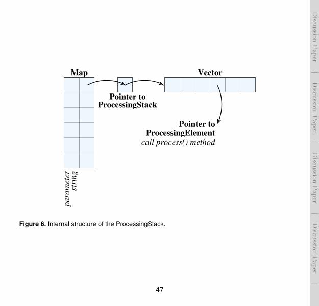
Discussion

Paper

|D

iscussionPaper

|D

iscussionPaper

|D

iscussionPaper

|

Pointer to

VectorMapst

rin

gp

ara

met

er

ProcessingElementcall process() method

Pointer toProcessingStack

Figure 6. Internal structure of the ProcessingStack.

47

Discussion

Paper

|D

iscussionPaper

|D

iscussionPaper

|D

iscussionPaper

|

1

2

3

4

Add fraction of accumulation −>

<− linearly interpolate

sum all samples until (insertion_index−1) −>

<− within a search window distance

Look for end point:

assuming a linear accumulation rate

Calculate fraction of accumulation −>

before the accumulation period −><− within the search window

Locate the requested timestamp, find start point:

��

��

��

��

��

��

��

��

��

��

��

��

��

��

��

��

search window

search window

search windowrequested timestamp requested timestamp

accumulation period

accumulation period

accumulation period

accumulation period

Figure 7. Resampling and reaccumulation operations.

48

Discussion

Paper

|D

iscussionPaper

|D

iscussionPaper

|D

iscussionPaper

|

500 1000 1500 2000 2500 3000

Elevation (m)

-5

0

5

10

15

20

25

Tem

per

ature

(°C

)

R = 0.52

1

2

3

500 1000 1500 2000 2500 3000

-5

0

5

10

15

20

25

Tem

per

ature

(°C

)

R = 0.72

Figure 8. Removing outliers for computing lapse rates.

49

Discussion

Paper

|D

iscussionPaper

|D

iscussionPaper

|D

iscussionPaper

|

Time required by each participant to write an empty filter and the filter required by the assignment.The plain lines represent the median.

Dur

atio

n (m

illise

cond

s)

0

20

40

60

80

Programming EnvironmentMeteoIO (STL) F95 (dynamic) C++ (STL) F95 (static) C (malloc)

I/O, line split, parsing, storageUnit conversioncopying to MeteoData, post processing

Figure 9. Performance when reading a SMET ASCII file with 1 year of hourly data into memory.

50

Discussion

Paper

|D

iscussionPaper

|D

iscussionPaper

|D

iscussionPaper

|

Dur

atio

n (s

econ

ds)

0

20

40

60

300

400

500

600

MeteoIO Version2.0.1 2.1.1 2.1.2 2.1.3 2.3.0 2.3.1 2.4.0 2.4.1 2.4.2

File I/OFilteringResamplingOther

Mar '11

Nov '12May '12

Dec '13 Feb '14

Sep '11

Oct '11

Mar '13Jul '14

Figure 10. Performance increase in MeteoIO (March 2011 until February 2014).

51

Discussion

Paper

|D

iscussionPaper

|D

iscussionPaper

|D

iscussionPaper

|

1 10 100 1 k 10 k 100 k 1 M 10 MNumber of cells

0.0001

0.001

0.01

0.1

1

10

100

1000

Tim

e (s

)

1*1 10*10 100*100 1k*1kgrid size

NoneCstCst_lapseIdwIdw_lapseODKrig_lapse

Figure 11. Benchmarks of some spatial interpolation algorithms for various grid sizes for seven inputstations (plain lines) and fourteen input stations (dotted lines).

52

Discussion

Paper

|D

iscussionPaper

|D

iscussionPaper

|D

iscussionPaper

|

One year,start of file

One year,end of file

Fourteen years 24 spatialinterpolations

0.1

1

10

time

(s)

15 stationsOne station7 stations

Figure 12.::::::::::::Benchmarks

::of

:::::::::different

::::::usage

:::::::::::scenarios:

:::::::reading

:::::one

:::::year

::of

:::::::hourly

:::::data

:::::from

::::the

:::::::::beginning

::of

::a:::::large

::::file,

::::::::reading

::::one

::::year

:::of

::::::hourly

:::::data

::at

::::the

::::end

::of

::a:::::large

::::file,

:::::::reading

:::::::::fourteen

:::::years

::of:::::::

hourly:::::data,

::::::::spatially

::::::::::::interpolating

:::::::seven

::::::::::::::meteorological

:::::::::::parameters

::::::every

::::hour

:::for

::a:::::day.

::::::These

:::::::::scenarios

::::are

:::::::::repeated

:::for

::::one

::::::station

::::and

:::::::fifteen

:::::::stations

:::::::::::::(respectively,

:::::files).

53

tex class copernicus.cls. date: 4 november 2014 meteoio 2 ... filemanuscript prepared for geosci....

Documents