text mining of news articles for stock price predictions
TRANSCRIPT

Master of Science in Computer ScienceJune 2011Pinar Öztürk, IDIArvid Holme, IDI
Submission date:Supervisor:Co-supervisor:
Norwegian University of Science and TechnologyDepartment of Computer and Information Science
Text Mining of News Articles for StockPrice Predictions
Kim-Georg Aase


1
Problem Description
This work is focused on the relationship between the news articles (breaking news) and stock prices.
The student will design and develop methods to analyze how and when the news articles influence the
stock market. News articles about Norwegian oil related companies and stock prices from “BW
Offshore Limited” (BWO), “DNO International” (DNO), “Frontline” (FRO), “Petroleum Geo-
Services” (PGS), “Seadrill” (SDRL), “Sevan Marine” (SEVAN), “Siem Offshore” (SIOFF), “Statoil”
(STL) and “TGS-NOPEC Geophysical Company” (TGS) will be crawled, preprocessed and the
important features in the text will be extracted to effectively represent the news in a form that allows
the application of computational techniques. This data will then be used to train text sense classifiers.
A prototype system that employs such classifiers will be developed to support the trader in taking
sell/buy decisions. Methods will be developed for automaticall sense-labeling of news that are
informed by the correlation between the changes in the stock prices and the breaking news.
Performance of the prototype decision support system will be compared with a chosen baseline
method for trade-related decision making.
Assignment given: 15. January 2011
Supervisors: Pinar Öztürk and Arvid Holme, IDI

2

3
Abstract
This thesis investigates the prediction of possible stock price changes immediately after news article
publications. This is done by automatic analysis of these news articles. Some background information
about financial trading theory and text mining is given in addition to an overview of earlier related
research in the field of automatic news article analyzes with the purpose of predicting future stock
prices.
In this thesis a system is designed and implemented to predict stock price trends for the time
immediately after the publication of news articles. This system consists mainly of four components.
The first component gathers news articles and stock prices automatically from internet. The second
component prepares the news articles by sending them to some document preprocessing steps and
finding relevant features before they are sent to a document representation process. The third
component categorizes the news articles into predefined categories, and finally the fourth component
applies appropriate trading strategies depending on the category of the news article.
This system requires a labeled data set to train the categorization component. This data set is labeled
automatically on the basis of the price trends directly after the news article publication. An additional
label refining step using clustering is added in an attempt to improve the labels given by the basic
method of labeling by price trends.
The findings indicate that categorization of news articles into positive, neutral, and negative categories
provides enough information for it to be used to forecast stock price trends. Experiments showed that
the label refining method greatly improves the performance of the system. It was also shown that the
timing of when to start the price trends used to label the data sets had a significant impact on the
results. Trading simulations performed with the systems managed to gain positive returns (profits) on
most of its trades. Some of the methods also managed to give better results than what trades performed
with the manually labeled data set did.

4

5
Contents
1 Introduction ..................................................................................................................................... 9
1.1 Motivation ............................................................................................................................... 9
1.2 Objectives and Hypotheses.................................................................................................... 10
1.3 Report Outline ....................................................................................................................... 11
2 Background ................................................................................................................................... 12
2.1 Trading Theory ...................................................................................................................... 12
2.1.1 Investing ........................................................................................................................ 12
2.1.2 Technical Analysis ........................................................................................................ 16
2.1.3 Fundamental Analysis ................................................................................................... 17
2.1.4 Efficient-Market Hypothesis ......................................................................................... 18
2.1.5 Random Walk Theory ................................................................................................... 19
2.1.6 News Articles Influence on Stock Markets ................................................................... 19
2.2 Relevant Text Mining Methods ............................................................................................. 21
2.2.1 Preprocessing ................................................................................................................. 21
2.2.2 Features Types ............................................................................................................... 23
2.2.3 Feature Selection Metrics (CHI).................................................................................... 24
2.2.4 Feature Reduction (SVD) .............................................................................................. 26
2.2.5 Document Representation ............................................................................................. 27
2.2.6 Classifier Learning (SVD) ............................................................................................. 31
2.2.7 Evaluation Metrics......................................................................................................... 33
3 Related Work on News-Stock Relationship Systems .................................................................... 35
3.1 Outline of Related Methods................................................................................................... 35
3.2 Training Set Creation ............................................................................................................ 35
3.3 Document Representation ..................................................................................................... 37
3.4 Architectures of News Based Trade Support Systems .......................................................... 38
3.4.1 NewsCAT ...................................................................................................................... 38
3.4.2 AZFinText ..................................................................................................................... 40
3.4.3 Falinouss ........................................................................................................................ 41
4 Scientific Approach ....................................................................................................................... 42
4.1 Approach Overview .............................................................................................................. 42
4.2 Data Acquisition .................................................................................................................... 43
4.2.1 Collection of News Articles .......................................................................................... 43
4.2.2 Collection of Stock Quotes ............................................................................................ 44
4.3 News Sentiment Labeling by Price Trends ........................................................................... 45
4.3.1 News Trend Labeling: Method One .............................................................................. 45
4.3.2 News Trend Labeling: Method Two ............................................................................. 46

6
4.3.3 Combining different labeled data sets ........................................................................... 46
4.3.4 Price trend timing .......................................................................................................... 46
4.3.5 Manually Labeled Set .................................................................................................... 47
4.4 Preparation of Data Set .......................................................................................................... 48
4.4.1 Document Preprocessing ............................................................................................... 48
4.4.2 Features ......................................................................................................................... 48
4.4.3 Document Elimination................................................................................................... 49
4.4.4 Document Representation ............................................................................................. 49
4.5 Label refining ........................................................................................................................ 50
4.5.1 K-Means clustering ....................................................................................................... 50
4.5.2 Restricted k-Means clustering method one ................................................................... 51
4.5.3 Restricted k-Means clustering method two ................................................................... 51
4.6 Classifier Learning ................................................................................................................ 51
4.7 Trading Engine ...................................................................................................................... 52
5 Experiment Preparation ................................................................................................................. 53
5.1 Evaluation methods ............................................................................................................... 53
5.1.1 Direct comparison of Manually Labeled Set with Automatically Generated Sets ........ 53
5.1.2 Classifier Evaluation ..................................................................................................... 53
5.1.3 Evaluation of Simulated Stock Trading ......................................................................... 53
5.2 Document Preprocessing and labeling .................................................................................. 54
5.3 Training and Test Sets ........................................................................................................... 54
5.4 Training Set Sources: Multiple Companies ........................................................................... 54
5.5 Feature Comparison .............................................................................................................. 55
5.6 Classifier Parameter Tuning .................................................................................................. 57
6 Experiments, Results and Analysis ............................................................................................... 59
6.1 Experiment 1: Timing of price trends for labeling ................................................................ 59
6.1.1 Results ........................................................................................................................... 60
6.1.2 Analysis ......................................................................................................................... 61
6.2 Experiment 2: Does label refinement help? .......................................................................... 62
6.2.1 Results ........................................................................................................................... 63
6.2.2 Analysis ......................................................................................................................... 66
6.3 Experiment 3: Trading engine ............................................................................................... 66
6.3.1 Results ........................................................................................................................... 67
6.3.2 Analysis ......................................................................................................................... 70
7 Conclusion and Future Work......................................................................................................... 72
7.1 Overview of Thesis ............................................................................................................... 72
7.2 Concluding Remarks ............................................................................................................. 72
7.3 Future Work .......................................................................................................................... 73

7
Bibliography .......................................................................................................................................... 75
Appendix A: News Article Example ..................................................................................................... 79
Appendix B: Examples of Evaluation Summaries ................................................................................ 81

8
List of Figures
FIGURE 2.1: Information on stock (Telenor) traded on Oslo Stock Exchange .................................................... 13
FIGURE 2.2 Truncation of matrices obtained through SVD. ............................................................................... 27
FIGURE 2.3: document vectors in vector space ................................................................................................... 30
FIGURE 2.4: SVM hyperplane and support vectors. Maximum margine. ........................................................... 31
FIGURE 2.5: SVM problem that is not linearly separable.................................................................................... 32
FIGURE 3.1: Trend, news alignment methods ..................................................................................................... 36
FIGURE 3.2: NewsCATarchitecture .................................................................................................................... 39
FIGURE 3.3: NewsCAT vs random - trade profit ................................................................................................ 39
FIGURE 3.4: AZFinText architecture .................................................................................................................. 40
FIGURE 4.1: The workflow of our proposed automatic news based trading approach ........................................ 43
FIGURE 4.2: News labeling from price trends method one - from NewsCAT .................................................... 45
FIGURE 4.3: NEWS LABELING FROM PRICE THRENDS METHOD Two .................................................. 46
FIGURE 5.1: Comparison of training sets with multiple and single companies (single = Statoil) ....................... 55
FIGURE 5.2: Feature comparison – CHI reduction 2000 features ....................................................................... 56
FIGURE 5.3: Feature comparison – SVD reduction 400 features ........................................................................ 56
FIGURE 5.4: Feature comparison – SVD reduction 1000 features ...................................................................... 57
FIGURE 5.5: SVM Parameter Tuning – white spots are parameter configurations that are not tested ................ 58
FIGURE 6.1: Comparing timing method “before” and “after” with the manually labeled set. ............................ 60
FIGURE 6.2: Classifying manually labeled data set ............................................................................................. 60
FIGURE 6.3: Classifying manually labeled data set – performance for positive and negative documents .......... 61
FIGURE 6.4: Compare Manually Labeled Set with Automatically Labeled Sets ................................................ 63
FIGURE 6.5: Classifying Test Set ........................................................................................................................ 64
FIGURE 6.6: Classifying Test Set – performance of positive and negative documents ....................................... 64
FIGURE 6.7: Classifying manaully labeled data set ............................................................................................. 65
FIGURE 6.8: Classifying manually labeled data set – performance of positive and negative documents............ 65
FIGURE 6.9: Average return per trade – performance of both buy and sell together ........................................... 67
FIGURE 6.10: Average return per trade – timing method before – dividing buy and sell ................................... 68
FIGURE 6.11: Average return per trade – timing method after – dividing buy and sell ...................................... 68
FIGURE 6.12: Average number of trades – timing menthod before and after – buy and sell .............................. 69
FIGURE 6.13: Average return per trade compared with average market return ................................................... 69
FIGURE 6.14: Percentage of the average maximum possible return per trade ..................................................... 70
List of Tables
TABLE 2.1 Examples of stock ticker symbols ..................................................................................................... 14
TABLE 2.2: CHI contingency table ...................................................................................................................... 25
TABLE 2.3Vector model with term counts as weights ......................................................................................... 28
TABLE 2.4: Vector model with tf-idf scores ........................................................................................................ 29
TABLE 2.5: Contingency table (TP, TN, FP, FN) ................................................................................................ 33
TABLE 3.1 Feature types from (Schumaker & Chen, 2006) ................................................................................ 37
TABLE 3.2: Return from Simulated trading (Schumaker & Chen, 2006) ............................................................ 37
TABLE 3.3: Percentage return on money invested (Schumaker & Chen, 2006) .................................................. 37
TABLE 3.4: Money invested (Schumaker & Chen, 2006) ................................................................................... 37
TABLE 3.5 AZFinText vs quant founds ............................................................................................................... 40
TABLE 6.1 Experiment 3 - manually labeled - trading returns ............................................................................ 67

9
1 Introduction
News articles written about companies serve the purpose of spreading information about the
companies, and this information then influence people either consciously or unconsciously in their
decision process when trading in the stock market. Annual and quarterly earnings, dividend
announcements, acquisitions, mergers, tender offers, stock splits, and major management changes, and
any substantive items of unusual or non-recurrent nature are examples of news items that are useful for
traders in their trading decisions. These types of news are usually published immediately as breaking
news and are often given to the press directly from the companies. News articles with other kinds of
information (e.g. political news) about companies are also important for traders, but they do not
necessarily originate from the companies themselves. With the immense growth of the internet in the
last decade, the amount of published news articles has experienced a similar rate of growth, which has
increased the amount of both useful and not so useful information about each company.
Information published in news articles influence, in a varying degree, the decisions of the stock
traders, especially if the given information is unexpected. It is important to analyze this information as
fast as possible so it can be used as help for trading decisions by traders before the market has had
time to adjust itself to the new information. This is a humongous task if done manually because of the
immense amount of information and the speed of which new information is published. This means that
an automatic system for analyzing news articles is needed.
Because of the internet, as mentioned above, there has been a huge growth of easily available textual
information over the last decade in the form of documents, news, blogs, forums, emails, and etc. This
increased amount of available textual information has lead to a research field devoted to knowledge
discovery in unstructured data (textual data) known as text mining (Konchady, 2006). Text mining
originates from the related field of data mining, which mines patterns from structured data instead of
unstructured. It is also related to other fields like information retrieval, web mining, statistics,
computational linguistics and natural language processing.
One important application of text mining is text sentiment analysis, also referred to as opinion mining.
This technique tries to discover the sentiment of a written text. This can be used to categorize text
documents into a set of predefined sentiment categories (e.g. positive or negative sentiment
categories), or it can be used to give the text a grade on a given scale (e.g. giving a text about a movie
review a score on a grade from one to ten). Sentiment analysis seems like a logical place to start when
applying text mining to analyze news articles. This is because positive news articles should have a
higher probability of positively influencing the stock price, while the opposite is true for negative
articles.
1.1 Motivation
The main purpose of this thesis is to investigate if and how text mining techniques can be used to
predicting the future trends of stock prices by analyzing news articles (breaking news). As we will see
later in chapter 3, researchers have already performed similar studies. However, this is still a small
field, but it is growing. There are more articles published on computational stock market prediction
that uses numbers like stock price, volumes, company income, company cost, and so on, instead of
textual information from news articles. It is important to investigate how stock markets react to
breaking news because if we know this we can create fast computerized systems that automatically
analysis new news articles before the market has had time to adjust itself to the new information.
Doing this opens up the possibility for making much more profit on stock trades, if it works.

10
There are some novel features in the system developed in this thesis that distinguishes it from other
existing articles in this field. The main difference is probably that it includes an extra process in hope
of improving the sentiment labels annunciated to the articles by first linking them with the price trend
for the related company after their publications (News followed by increased prices are positive and
the opposite ones are negative). Three algorithms based on clustering techniques were added and
compared for this extra step in an attempt to improve the automatic labeling process. This thesis also
adds methods mentioned in other related and unrelated articles but which are not commonly used in
these kinds of systems, like bigrams as features, feature reduction by using SVD, selecting only
documents containing significant features and comparing the result with a manually labeled set.
1.2 Objectives and Hypotheses
The objectives and hypotheses for the thesis are formulated as follows.
Objectives
1- Study existing systems for automatically analyzing financial news articles with main focus on
systems that uses the sentiment of news articles in their prediction of future price trends.
2- Investigate text mining methods that might be used in an attempt to create an improved
system.
3- Design, implement and evaluate a system that uses sentiment analysis on news articles to
automatically generate trading signals.
Hypothesizes
1- When the stock trading is done from signals generated from sentiment analysis of news
articles, then the profit is better compared to what a random trader gives. Or in other words, a
news based trader will give positive profits over time.
2- A classifier trained on an automatically created training set performs on the same level as
humans at predicting how trends will move after news articles are published.
3- A training set of news articles for the sentiment classifier might be automatically created and
labeled by looking at how the price for the related company changes after the article is
published.
4- A training set created by looking at price trends after the news article is published is improved
by running it by a clustering based algorithm for label refining.
5- The timing of when to start the price trend when it is used for labeling news articles for the
training set is important. Starting the price trend a little before the news article is published
gives better results since it is certain to capture the early price adjustments right after the news
is published.

11
1.3 Report Outline
This thesis consists of seven chapters including the introduction and the conclusion. Chapter 2
explains some general background about trading theory (section 2.1) and about text mining (section
2.2) that are useful for understanding the following chapters. Chapter 3 gives an overview of some
related research on the subject of news based trading systems. The general structure of the related
systems are described and some of the more important and common aspects are described in more
detail. Chapter 4 describes the framework developed in this thesis. Chapter 5 prepares the system for
experimenting by choosing system parameters and explaining data handling and the experiment
evaluation methods. In chapter 6 the conducted experiments are described and the experimental results
are analyzed. The thesis concludes with a summary of experimental results and future research
directions in chapter 7. Two appendixes are also included. Appendix A shows an example of a news
article and its features, and appendix B show some examples of evaluation summaries.

12
2 Background
2.1 Trading Theory
This thesis assumes no prior knowledge of finance and trading theory on the part of the reader, it is
therefore appropriate to provide some basic background of financial trading theory. This section
explains some key financial trading concepts which should make it easier to understand the rest of this
thesis.
2.1.1 Investing
This section briefly introduces some central concepts of investment theory. Its purpose is to give a
basic understanding of how investment decisions are done on a basic level. In the field of finance,
investment generally refers to the act of using capital (i.e. money) to buy some type of asset expected
to generate a profit for the investor over time.
The focus of this report is on stocks, which is a specific type of financial asset, and how stock prices
are affected by financial news articles. The theory discussed and developed in the following chapters
in this thesis should in theory be possible to apply to many other types of liquid assets (a liquid asset is
an asset that has many sellers and buyers). Examples of liquid assets are stocks, bonds1, currencies
2,
commodities3 and mutual funds
4, but this thesis focuses only on stocks.
Stocks
A stock is a type of financial asset that denotes part ownership on the assets and profits of a company.
It also entitles the owner of the stock to receive dividends if the company chooses to pay some of their
profits to the shareholders. Typically, ownership of a stock also gives the investor a right to vote on
corporate decisions at shareholder meetings.
Stock exchanges
Stocks are usually traded at one or more stock exchanges. The exchange receives an influx of orders to
buy or sell a given volume of a stock at a given price, which are matched together making a trade
when the price of a buy order matches the price of a sell order.
Historically, stock exchanges have been physical places where stock brokers placed orders to buy or
sell stocks in person, but with the technological advances more and more stock exchanges have
become purely electronical. The world’s largest exchange, the New York Stock Exchange (NYSE),
still has a physical trading floor (although most orders are now electronically entered) (New york
stock exchange: Wikipedia). Another popular exchange, NASDAQ, is managed completely
electronically (Berk & DeMarzo, 2007, s. 13). In Norway, the largest stock exchange is the Oslo Stock
Exchange (OSE), which is where the stocks in this thesis are from, also trade stocks electronically
(Oslo stock exchange: Wikipedia).
1 A bond is a formal contract to repay borrowed money with interest at fixed intervals. (Arthur & Sheffrin, 2003)
2 In economics, currency refers to physical objects generally accepted as a medium of exchange. (Currency:
Wikipedia) 3 Commodities are goods for which there is a demand, but which is supplied without qualitative differentiation
across a market. A commodity is treated by the market as equivalent or nearly so no matter who produces it.
Examples are petroleum and copper. (Arthur & Sheffrin, 2003) 4 A mutual fund is a type of investment company that pools money from many investors and invests the money
in stocks, bonds, money-market instruments, other securities, or even cash. (Mutual Funds: U.S Securities and
Exchanges Commission)

13
FIGURE 2.1: Information on stock (Telenor) traded on Oslo Stock Exchange
Basic stock information
FIGURE 2.1 shows an example of relevant information for a stock traded on the Oslo Stock
Exchange, taken from the OSE website. The stock in the example is of the Norwegian corporation
Telenor. Some of the information presented is:
- The current bidding price (the highest current buy order) and the asking price (the lowest
current sell order).
- An order depth which shows what volumes of (number of) stocks has been ordered to buy or
sell at a given price.
- The last trading price, which is the most recent price at which a buy and sell order were
matched together to make a trade. There is also a list called “Last trades" which shows several
of the most recent trades.
- The high and low prices show the highest and lowest prices at which the stocks have traded
throughout the day.
- The “Profit % today" figure shows what percentage the price has moved since the last price
traded, the close, of the previous day. This figure is commonly referred to as the intraday
return from the given stocks.
- There is also a table called “Historical prices", where you can see the return from the stocks
since last week, last month, the beginning of the current year and one year ago exactly. This
table also shows the high and low prices over the respective time periods.
- The market capitalization figure shows the current total value of the company as measured by
the last price at which it was traded multiplied by the total number of outstanding stocks in the
company.
In addition to the figures given in this example, some other basic statistics of interesting includes:
- The volume of stocks that have been traded throughout the day. The volume of the traded
stocks gives a good measure of the liquidity of the stock, indicating how easy it would be for
any individual investor to buy or sell a large number of stocks in the market.
- The opening price, simply referred to as open, for the stock in that day (i.e. the price of the
first trade of the stock in the trading day).

14
Ticker symbols
All stocks that are publicly traded are given a short abbreviation called a ticker symbol used to
uniquely identify them on a particular market. Because a given ticker symbol may refer to a different
stock on a different stock exchange, it is not uncommon to prefix the ticker symbol with an
abbreviation that identifies the exchange on which it is traded in order to avoid confusion. TABLE
2.1contains a few examples of what ticker symbols are used to identify certain stocks.
Ticker symbol Corporation Stock exchange
GE
GOOG
MSFT
REC
STL TEL TABLE 2.1 Examples of stock ticker symbols
Stock market indexes
A stock market index is a method of measuring the price movements of a collection of stocks.
Different indexes measure different collections of stocks using different formulas. Indexes are useful
to investors because they give a benchmark by which one can compare the returns of individual
stocks.
The popular Dow Jones Industrial Average (DJIA) index measures the collective return of 30 large-
cap (large market capitalization) stocks traded on either the NYSE or the NASDAQ, using a price
weighting. This means it is computed by taking a weighted average of the prices of its 30 constituent
stocks where each stock is weighted proportionally to its price.
Another heavily quoted index is the S&P 500 which until recently was a market-value weighted index
composed of 500 large-cap stocks traded in the US. A market-value weighted index is computed as a
weighted average where each component stock is weighted proportionally to its market capitalization.
Since 2005, the index has transitioned from being market-valued to becoming oat-weighted, which in
short means that only the capitalization of the stocks that are available for public trading are taken into
account.
Stock options
A stock option is a type of financial contract whose value is tied to the future value of a stock. There
are two main types of options:
Call option: A call option gives the owner of the option a right to purchase stocks at a given price
(the strike price) on a given date in the future. If the actual market price of the stock is
higher than the strike price at that time, he can then immediately sell the stocks to the
market for a profit. If not, the option is valueless.
Put option: A put option is a similar contract, but instead of the right to buy, it gives the owner of
the option a right to sell stocks at a given strike price on a given future date. This
means its value at that date is equal to the difference between the strike price and the
market price (i.e. the lower the market price the better).

15
Stock options are traded on most major stock exchanges. To illustrate with an example, consider the
STL0M145 option contract traded on the OSE. This is a put option which gives the owner the right to
sell shares of Statoil (STL) for 145 NOK in January of 2010. As of 28.11.09 this option was last traded
at 7.50 NOK, meaning it will only be profitable if the share price of Statoil in January 2010 is lower
than 145 – 7.5 = 137.5.
Stock options are popular to investors because they can potentially make a large profit on a small
investment. However, they are also a lot more risky than just buying the stock, because they can easily
loose all their value.
Long and Short Positions
Long position
As already discussed, an investment in an asset such as stocks usually involves the following steps:
buying the stock, owning the stock for some period of time, and finally selling it back to the market. In
financial terms, investing in this manner is known as taking a long position in the stock. More
generally, an investor is said to have a long position in a stock when he owns one or more units of the
stock.
Short position
Sometimes, an investor might believe that a given stock will have a negative return in the future (that
the price will fall). As mentioned earlier, one way to profit from such a downward move might be to
buy a put option for the stock. Another way to profit from falling prices is by taking a short position in
the stock. Taking a short position in a stock generally involves the following steps:
1. First, you borrow the amount of stocks you wish to go short. For a private investor, this stock
loan is typically carried out automatically through their stock broker.
2. Immediately after borrowing the stocks, you sell them to the market for the current price p0.
3. After some time, hopefully, the price has fallen down and you buy the same amount of stocks
back from the market at the lower price p1.
4. You return the stocks back to their original owner step 1.
As you can see, this investment is profitable as long as p0 > p1 (i.e. the share price has gone lower).
Risk comparison
The potential for losing money is far greater for the short position than for the long position. This is
because the future price of the stock can grow unboundedly high, meaning that in an extreme scenario
you might have to pay many times the original price to repurchase the stocks, giving you a loss of far
more than 100%. With a long position, there is no way you could lose more than 100% of the money
you invest, and this would only happen in the scenario that the company went bankrupt (unless you're
using leverage, which will be discussed shortly).

16
2.1.2 Technical Analysis
In its purest form, technical analysis only uses historical and current price and volume values to
predict future price moves. This means that technical analysis mainly uses models and trading rules
based on price and volume transformations, such as the moving averages5, relative strength index
6
(RSI) and price correlations. It can also look for chart patterns7, such as “head and shoulders”
8,
triangles, trend lines and Elliot waves9. Some different definitions of technical analysis, taken from
different sources, are:
Technical analysis is the study of market action, primarily through the use of charts, for the
purpose of forecasting future price trends. (Murphy, 1999)
Technical analysis is a security analysis discipline for forecasting the future direction of prices
through the study of past market data, primarily price and volume. (Technical analysis:
Wikipedia)
Technical Analysis is the science of recording, usually in graphic form, the actual history of
trading (price changes, volume of transactions, etc.) in a certain stock or in "the Averages" and
then deducing from that pictured history the probable future trend. (Meyers, 2002)
Principles
Classical technical analysis are based upon three main principles, and they are; (I) Market action
discounts everything, (II) Prices move in trends, and (III) History tends to repeat itself.
Market Action Discounts Everything
The statement "market action discounts everything" forms what is probably the most important
cornerstone of technical analysis. The technician believes that anything that can possibly affect the
price - fundamentally, politically, psychologically, or otherwise - is automatically reflected in the price
of the market.
Prices Move In Trends
The concept of trends is absolutely essential to the technical approach. Technicians say that markets
trend up, down, or sideways (flat). This basic definition of price trends is the one put forward by Dow
Theory.
5 Moving average: Given a series of numbers and a fixed subset size, the moving average can be found by first
calculating the average of the first subset. Next the subset is shifted one step forward, and the average of this
new subset is calculated. This process is repeated over the entire data series. A line is then plotted by connecting
these calculated values to create the moving average. 6 RSI measure the velocity and magnitude of directional price movements. The RSI is classified as a momentum
oscillator, where the momentum is the rate of the rise or fall in price. 7 Chart patterns are a pattern within price charts. They are patterns which naturally occur and repeats over time.
Chart patterns are used as either reversal or continuation signals. 8 Head and Shoulders patterns consist of a left shoulder, a head (higher peek than the shoulders), and a right
shoulder and a line drawn as the neckline between the shoulder. The price is likely to reverse its direction if the
price crosses over the neckline after the left shoulder. 9 Elliott proposed that market prices unfold in specific patterns, which practitioners today call Elliott waves.
Elliott stated that "because man is subject to rhythmical procedure, calculations having to do with his activities
can be projected far into the future with a justification and certainty heretofore unattainable. (Elliott, 1994)

17
Prices move in trends and trends tend to continue until something happens that changes the demand
and supply balance. This can be seen as an adaption of Newton's first law, "A body persist its state of
rest or of uniform motion unless acted upon by an external unbalanced force". These "external" forces
can be technical signals such as reversal patterns or breakouts. The goal in this trend-following
approach is for the technician to get in on an existing trend as early as possible and ride on it until it
shows signs of reversing.
History Tends to Repeat Itself
Technicians believe that investors collectively repeat the behavior of the investors that preceded them.
Because investor behavior repeats itself so often, technicians believe that recognizable and often
predictable patterns will emerge. The key to understanding the future therefore lies in studying the
past.
2.1.3 Fundamental Analysis
Fundamental analysis of a business involves analyzing its financial data to get some insight on
whether it is overvalued or undervalued. This is done by analyzing historical and present economic
data to do a financial forecast of the business. The intrinsic value of the business is found by doing a
fundamental analysis which consist of three main steps; (I) economic analysis, (II) industry analysis
and (III) company analysis. If the intrinsic value is higher than the market price it is recommended to
buy stocks, if it is equal to market price then it is best to hold your shares, and if it is less than the
market price then it’s a selling signal.
Fundamental analysis maintains that markets may misprice an asset in the short run but that the
"correct" price will eventually be reached. Profits can be made by trading the mispriced security and
then waiting for the market to recognize its "mistake" and reprises the security. (Fundamental analysis:
Wikipedia)
Procedures
All publicly traded companies release reports on their financial performance on a regular basis
(usually once every quarter with a larger annual report). These reports typically include different types
of financial statements, the most significant being: the balance sheet10
, the income statement11
, the
cash flow statement12
and dividend paid. The fundamental analysis of a business' health starts with
analysis of some of these financial statements.
The determined growth rates and risk levels are used in various valuation models. The foremost is the
discounted cash flow model13
, which calculates the present value of the future. The amount of debt is
10
A balance sheet is often described as a "snapshot of a company's financial condition". It is a summary of the
financial balances of a company. (Berk & DeMarzo, 2007) 11
Income statement is a company's financial statement that indicates how the revenue is transformed into the net
income. It displays the revenues for a specified time period, and the cost and expenses charged against these
revenues, including write-offs and taxes. (Berk & DeMarzo, 2007) 12
Cash flow statements are essentially concerned with the flow of cash in and cash out of the business. It is a
financial statement that shows how changes in balance sheets and income affect cash flow. (Berk & DeMarzo,
2007) 13
Discounted cash flow (DCF) analysis is a method of valuing a project, company, or asset using the concepts of
the time value of money. All future cash flows are estimated and discounted and added together to give their
present value. (Discounted cash flow: Wikipedia) (Jennergren, 2008)

18
also a major consideration in determining a company's health. It can be quickly assessed using the debt
to equity ratio14
and the current ratio15
. (Fundamental analysis: Wikipedia)
Some other methods often used when performing a fundamental analysis are the popular P/E and PEG
ratios. The P/E (price/earnings) ratio is the price of one share divided on the company profit per share,
while the PEG (Price/Earnings to Growth ratio) includes the feature expected growth of the company
so a high- growing company won’t appear overvalued to others.
2.1.4 Efficient-Market Hypothesis
The efficient-market hypothesis (EMH) states that market prices always reflects all available
information, or in other words, financial markets are informational efficient. This means that no one
can consistently achieve greater returns than that of the average market returns, not even if they are
given all the publically published information that are available at the time of investment.
The EMH is divided into three different hypotheses: weak form efficiency, semi-strong form
efficiency, and strong form efficiency, each of which has different implications for how the market
works.
Weak form efficiency states that future prices cannot be predicted from analyzing historical prices. In
other words, excess returns, or profits, cannot be gained in the long run by using investment strategies
based on historical prices or other historical forms of data. This means that technical analysis will not
be able to consistently produce excess returns. This is because one of the main principles vital to
technical analysis states that history tends to repeat itself. It states that stock prices exhibit no serial
dependencies, meaning that there exist no "patterns" to asset prices, which is especially important for
chartists which is a subfield under technical analysis. Weak form efficiency states that all future price
movements follow a random walk, unless there is some change in some fundamental information. It
does not state that prices adjust immediately in the advent of new fundamental information, which
means that some forms of Fundamental analysis and also news article analysis might provide excess
returns. This is because they trades on new information and does not use any historical information to
look for patterns.
Semi-strong form efficiency implies that share prices adjust in an unbiased fashion to new publicly
available information very rapidly such that no excess returns can be earned by trading on that
information. This form of EMH implies that fundamental analysis, technical analysis nor news trading
will be able to reliably produce excess return over time.
In strong-form efficiency, stock prices reflect all information, public and private, and no one can earn
excess returns. According to this form of EMH, those traders that are consistently getting profitable
return are only lucky since they are among the randomly selected few that are.
There has been a lot of criticism against the EMH. Manly because it assumes that investors always
behave rationally, but many behavioral economists argue that the presences of cognitive biases (such
14
The debt-to-equity ratio (D/E) is a financial ratio indicating the relative proportion of shareholders' equity and
debt used to finance a company's assets. (Debt-to-equity ratio: Wikipedia) 15
Current ratio is a financial ratio that measures whether or not a firm has enough resources to pay its debts over
the next 12 months. (Current ratio: Wikipedia)

19
as confirmation bias16
, the bandwagon effect17
, hyperbolic discounting18
, and irrational escalation of
commitment19
) negate the validity of this assumption.
Fore hypothesis 1 in this thesis to be true, the EMH has to be false. If it is not, only the week form
EMH can be true. If the semi-strong or the strong form EMH is true, then hypothesis 1 will be false.
2.1.5 Random Walk Theory
The theory of the random walk hypothesis (Cootner, 1964) claims that stock market prices changes
according to a random walk and, consequently, prices cannot be predicted. Therefore, it is impossible
to consistently outperform the average market return. This theory is based on the efficient-market
hypothesis (EMH), which says that prices fluctuate randomly about their intrinsic value. It also holds
that the best trading strategy to follow would be a simple “buy and hold” instead of any attempt to
“beat the market”.
The primary experiment conducted for this theory was to draw a price graph randomly and have some
chartists (technical analysts that analysis price charts) analyze it. The price graph started from an
initial value of fifty dollars and all future movements (ups and downs) was chosen by performing a
coin flip (fifty-fifty chance for each movement). The chartist, after analyzing the graph, found signs
that made him recommend buying. This is then used to argue that the market and stocks could be just
as random as flipping a coin.
There have been many researchers that have attempted to produce falsifications of the EMH and the
random walk hypothesis, with mixed results. One of the most commonly mentioned is the book “A
Non-Random Walk Down Wall Street” (Lo & MacKinlay, 1999) which describes a statistical model
claiming to provided significant empirical evidence against the random walk theory.
2.1.6 News Articles Influence on Stock Markets
The basic strategy for news based trading is to buy a stock from companies that has just gotten good
news published about them self, or short sell on bad news. Strong and unexpected positive or negative
events provide enormous volatility in a stock and gives therefore great chances for quick profits, or
losses if they are interpreted wrongly. Determining whether news was "good" (positive) or "bad"
(negative) should be determined by the price trend after the news article was published because the
market reaction may not match the tone of the news itself. The most common cause for this is when
rumors or estimates of the event, like those issued by market and industry analysts, were already
circulated before the official news release, and prices have already adjusted them self in anticipation
of the official news release.
16
Confirmation bias is a tendency people have to favor information that confirms their preconceptions or
hypotheses regardless of whether the information is true. Consequently, people gathers evidence and recall
information from memory in a selectively fashion. (Plous, 1993) 17
The bandwagon effect states that people often do and believe things merely because many other people do and
believe the same things. (Bandwagon effect: Wikipedia) 18
Given two similar rewards the hyperbolic discounting states that humans show a preference for the one that
arrives sooner rather than the one that arrives later. Humans are said to discount the value of the later reward, by
a factor that increases with the length of the delay. (Hyperbolic discounting: Wikipedia) 19
Irrational escalation of commitment is a term frequently used to refer to a situation in which people can make
irrational decisions based upon rational decisions in the past or to justify actions already taken. It’s a
phenomenon where people justify increased investment in a decision, based on the cumulative prior investment,
despite new evidence suggesting that the cost, starting today, of continuing the decision outweighs the expected
benefit. (Escalation of commitment: Wikipedia)

20
For it to be possible for traders trading on news articles to gain excess returns over time all but the
week form efficiency of the EMH (see section 2.1.4) has to be false. If the semi strong or the strong
form efficiency EMH is true then it is impossible to gain excess returns over time with news based
trading.
The number of traded stocks has been shown to be positively or negatively affected by economic news
publications (Chan, Chui, & Kwok, 2001). It is also found that both political and economical news
articles affect trading activities such as price volatility, number of stocks traded, and trade frequency
(Chan, Chui, & Kwok, 2001). Country specific news articles occupying at least two columns on The
New York Times front pages has been shown to affect the trading actions of closed-end country
funds20
. News articles appearing on the front page of the Shout China Morning Post has been shown to
increase the volatility in the Hong Kong stock market (Chan & John-Wei, 1996). The number of
relevant headlines reported by Dow Jones and Reuter’s News Service per time unit has also been
shown to affect the volume (volatility) on the related stocks (Mitchell & Mulherin, 1994) (Berry &
Howe, 1994). All this is strong evidence against the EMH, at least for the strong and semi-strong
forms. This means that there should be possible to create a system that automatically analysis news
articles and returns a trade signal (buy, hold, or sell) based the results from its analysis.
20
A closed-end fund is a collective investment scheme with a limited number of shares. It is called a closed-end
fund because new shares are rarely issued once the fund has launched, and because shares are not normally
redeemable for cash or securities until the fund liquidates. (Closed-end fund: Wikipedia) A country fund is an
international mutual fund with a portfolio that consists entirely of securities, generally stocks, of companies
located exclusively in a given country. (Country fund: Investopedia) (closed-end-country-funds: financial-
education) (Klibanoff, Lamont, & Wizman, 1998)

21
2.2 Relevant Text Mining Methods
This section briefly describes the text mining methods used by the trade support and analysis systems.
It`s primarily goal is to describe the methods used or planed to be used in the system developed in this
thesis, but it also describes some methods not used in this system but which are used by other news
based trade support systems that are described in chapter 3.
Text mining (Konchady, 2006) (Text mining: Wikipedia) refers to the process of deriving high-quality
information from text. High quality in text mining usually refers to some combination of relevance,
novelty, and interestingness. Text mining usually involves the process of structuring the input text,
deriving patterns within the structured data, and finally evaluation and interpretation of the output.
Typical text mining tasks include text categorization21
, text clustering22
, concept/entity extraction,
production of granular taxonomies, sentiment analysis23
, document summarization24
, and entity
relation modeling. Text mining has been applied in many different areas, some being; biomedical
applications (e.g. identification of biological entities, association of gene clusters, automatic extraction
of protein interactions and associations of proteins to functional concepts), software and applications,
online media applications, marketing applications (e.g. customer relationship management), and
sentiment analysis (e.g. customer sentiments on movies and products).
2.2.1 Preprocessing
Text preprocessing is the process of making clear each language structure and to eliminate as much as
possible the language dependent factors. (Wang & Wang, 2005) There are many different tasks under
preprocessing, but some of the most common ones are tokenization, stop-word removal and word
stemming.
Tokenizing
Tokenization is the process of splitting a text stream into symbols, words, phrases, or other meaningful
elements called tokens. These tokens are used further text mining techniques. Word tokens are
typically sent to preprocessing stages like stop-word removal and stemming, which are described later.
They are also used as input for feature extraction processes.
There are many ways of tokenizing text streams into tokens. A simple method would be just to split
the text on blank spaces, but better methods also takes punctuation and other sings into consideration.
The tokenizing method used in this thesis would tokenize the following text string:
"Hello! This is test number 11. It tests the word_punct-tokenizer!@ test66"
21
The Document categorization (classification) task is to assign an electronic document to one or more
categories, based on its contents. (Document classification: Wikipedia) 22
Text clustering is closely related to the concept of data clustering. Document clustering is a more specific
technique for unsupervised document organization, automatic topic extraction and fast information retrieval or
filtering. (Document clustering: Wikipedia) Clustering is the assignment of a set of observations into subsets
(called clusters) so that observations in the same cluster are similar in some sense. (Cluster analysis: Wikipedia) 23
Sentiment analysis aims to determine the attitude of a speaker or a writer with respect to some topic or the
overall tonality of a document. (Sentiment analysis: Wikipedia) 24
Automatic summarization is the computation of a shortened version of the original text. The product of this
procedure still contains the most important parts. (Automatic summarization: Wikipedia)

22
First by splitting it on blank space, then this is followed by splitting it on most special characters. The
tokenized string would then consist of the following tokens.
['Hello', '!', 'This', 'is', 'test', 'number', '11', '.', 'It', 'tests', 'the', 'word_punct', '-', 'tokenizer', '!@',
'test66']
Stop-Word Removal
Stop words are high frequency words of a language that don’t carry any significant information on
their own. These words are often removed at the preprocessing stage to reduce the number of features
(se section 2.2.2 for features), thus reducing the amount of noise. However, stop words can together
with other words contain a significant amount of information. Which means that in some situations,
like when searching for phrases (e.g. “To be or not to be”) or names (e.g. “The The” or “The Who”),
the stop-words are sometimes kept and not removed. Closed class words like articles, pronouns,
prepositions and conjunctions are usually included in stop-words lists. Some of the more frequently
used open class words like auxiliary verbs are also included. It is also possible to create domain
dependant stop word lists by filtering out high and low frequency words, or by using some statistical
measure like information gain or chi-square to filter out the less informative words. During the
removal process all the words that exist in the given stop word list are removed from the source
documents.
Stemming
In linguistic morphology, stemming is the reduction of a word from its inflected form to its root, stem
or base form. The stem does not need to be the words morphological root, it`s usually enough that
related words map to the same stem, even if this stem is not in itself a valid root. It is a common
procedure to use in information retrieval, natural language processing and other methods dealing with
text analysis to discover the semantic similarity between the different morphological variants of a
word. This means that and article that for example uses the word “walks” and another using the word
“walking” will both have their word reduced to its root which is for both of them “walk”. By doing
this they have both gained a similar feature instead of having two features that the computer would see
as totally different even when they for humans clearly have a high semantic similarity. Supporters for
word stemming argue that it has the effect of reducing the dimensionality of features which makes the
data less sparse and faster to work with, and that it can be helpful to promote the effectiveness of a text
classifier. But some experimental results showed that stemming sometimes might be harmful to the
effectiveness of a text classifier(Baker & McCallum, 1998).
Some example of words that are or might be stemmed:
Stemmer, stemming, stemmed stem
Cats, catty, catlike cat
Fishing, fishes, fished, fisher fish
The best known stemming algorithm is probably the Porter stemmer. It uses a set of language specific
rules to transform a word into its base form. However in this paper a different stemmer for Norwegian
is written in the Snowball language developed by Porter. Snowball is a string-handling programming
language where the rules for the stemming algorithm can be easily expressed in a natural way.

23
2.2.2 Features Types
Before text documents can be analyzed by text mining techniques, they must undergo a special
processing step known as feature extraction. This process takes the preprocessed text documents and
produces a set of features representing each document. Text features may be surface level lexical
features, or semantic or other higher-level features. Surface level lexical features are word–based
features that can be observed directly in the documents. Semantic features or higher-level features are
extracted from the surface level lexical features. Statistical techniques, such as singular value
decomposition (SVD), which is mentioned later in this chapter, topic modeling, and random
projection, are important in solving this kind of problem. Higher-order features can greatly improve
the quality of information retrieval, classification, and clustering tasks. These higher-order features are
also often used as feature reduction techniques.
Unigrams
Unigrams are N-Grams25
of size one, ore in other words, they consists of one single word. Another
name used for unigram features are bag of words feature sets. Feature sets made from unigrams are
made of all the selected single words that are left after the documents preprocessing steps. Despite its
simplicity, this feature type has proven successful in text classification and word sense disambiguation
(Mooney, 1996).
Bigrams
Bigrams are N-Grams of size two. Bigrams are a consecutive sequence of two words, and are very
commonly used as the basis for simple statistical analysis of text. Bigrams captures more of the
underlying sentence structure and contain more information than what unigrams do. This might help to
improve the classification of the news article sentiment. Take the following imaginative articles:
D1: “X has changed their recommendation for company Y from sell to buy.”
D2: “X has changed their recommendation for company Y from buy to sell.”
The unigram representations of these two documents are exactly the same, but their sentiment are
clearly not the same. However, by using bigrams, four following bigrams; “from sell”, “to buy”, “from
buy”, and “to sell” are different. These features are therefore important in classifying the sentiment of
the articles D1 and D2.
Noun Phrases
A noun phrase is a phrase based on nouns, pronouns, or other noun-like words, and it can optionally
be accompanied by modifiers such as adjectives. Noun phrases normally consist of a head noun, which
is optionally modified. Some examples of noun phrases are: blue car, where I live, blond girl, and the
butler.
Noun phrases can be used to get more informative features than only single words and less important
word are not included as features. To be able to extract noun phrases the text has to be tagged with a
part-of-speech tagger(Part-of-speech tagging: Wikipedia) first. In a tagged document each word is
tagged with tokens like noun, verb, adjective, etc. When the document is tagged the tags can be used
to extract noun phrases.
25
An N-Gram is a subsequence of n items from a given sequence. In this thesis the items are words.

24
Proper Nouns
Proper nouns(Mark & Larry, 2005), also called proper names, are nouns that represent unique entities,
such as New York, John Smith, or Microsoft. They are distinguished from common nouns which
describe classes of entities, such as the entities city, planet, person or corporation. Proper nouns are
usually capitalized in English and most other languages using the Latin alphabet. Proper nouns are a
subset of the set of noun phrases.
Name Entities
Name entities are special name entities, such as person names, locations, and organizations, in text
documents. It is somewhat similar to proper nouns, but not as strict. Name entities can also include
dates, times, and other numerical information. Name entities are often found by using statistical
learning systems.
2.2.3 Feature Selection Metrics (CHI)
Feature selection is crucial to make the classification tasks more efficient and precise because textual
data contains a very high-dimensional degree of features. Thus feature selection is a common way to
reduce this high-dimensionality by only selecting the most important features. Some common feature
selection matrices are information gain26
, mutual information27
, odds ratio28
, term strength29
,
correlation coefficient, and chi-square (Taşcı & Güngör, 2008) (Forman, 2003). In this thesis we have
chosen chi-square (CHI). The CHI does not give the best results of the feature selection methods, but
it is among the better. It can also work with more than two values, and this thesis uses three.
Chi-Square Statistic (CHI)
A chi-square (X2) statistic is used as a test of independence between each feature and the categories.
When the chi-squared value is zero it means that the feature is independent of the category and the
larger it gets the more dependent it is on the category. Feature selection can thus be done by only
selecting features that has ha chi-square value higher than a given threshold, while the rest of the
features can be discarded since they are independent of the categories, which means they have no
significance.
To find each terms CHI value a contingency table is needed for each of them. Since this thesis
operates with three categories, 2×3 contingency tables are constructed to determine the terms CHI
values. This is in fact similar to a chi-square distribution with two degrees of freedom to judge
extremeness. The chi-square value is found by the following formula:
26
Information gain measures the number of bits of information obtained for category prediction by knowing the
presence or absence of a term/feature in a document. 27
The mutual information of two random variables is a quantity that measures the mutual dependence of the two
variables. If the mutual information score is 0, then the two random variables are independent. (Mutual
information: Wikipedia) 28
The odds ratio is a measure of effect size, describing the strength of association or non-independence between
two binary data values. (Odds ratio: Wikipedia) Effect size is a measure of the strength of the relationship
between two variables in a statistical population, or a sample-based estimate of that quantity. 29
Term strength estimates the term/feature importance based on how commonly a term is likely to appear in
closely related documents. It uses a training set of documents to find document pairs that has a similarity score
above a given threshold.

25
Here F0 denotes the frequency of the observed data, and the Fe denotes the frequency of the expected
values. The 2×3 contingency table used for this calculation looks something like this:
Positive Neutral Negative Row Totals
Category have feature A B C A+B+C
Category do not have feature D E F S+E+F
Column Totals A+D B+E C+F Q+B+C+D+E+F=N TABLE 2.2: CHI contingency table
In TABLE 2.2 the cells A, B, and C shows how many documents that contains the given feature for
each of the three categories, positive, neutral and negative has. The cells D, E, and F on the other hand
show how many documents that does not contain the given feature. These cells contain the observed
values F0.
The next step is to calculate the expected values for each cell in the contingency table. This can be
done by multiplying the row totals with the column totals and dividing it on the grand total. As an
example, the calculation for the expected value for cell A looks like this:
The expected value is found for each of the cells, then (F0 – Fe)2/Fe is also found for each cell, and then
they are summed up to get the CHI value. Then the degrees of freedom are found by this formula:
And the chi-square calculation used in this thesis has 2 degrees of freedom. The minimum CHI value a
term can have for it to still be significant is 5.991. If a term has a value less than this it means it is
independent, and thus not of any importance when categorizing the documents. This value is found by
looking up in a chi-square distribution table where alpha is chosen to be 0.05 and the degrees of
freedom that was found earlier is 2.
The chi-square values are normalized, however this normalization breaks down and behaves erratically
if any cell in the contingency table is lightly populated (less than five), which is the case for low
frequency terms. This is simply solved in this thesis by giving all terms that has a cell with a value less
than five a CHI value of zero.

26
2.2.4 Feature Reduction (SVD)
Feature reduction is as the name implies the process of reducing the number of features that are used
for representing text documents. This is an important process since to many features affect the
performance of classifiers and other text mining methods like document clustering and similarity
measures. Feature reduction can be done by a simple feature selection process where the best features
are selected and the rest are removed, or it is possible to fit methods that discover latent variables as
feature reduction methods. Methods that discover latent variables are latent semantic analysis (LSA)
(Deerwester, Dumais, Furnas, Landauer, & Harshman, 1990) which uses singular value decomposition
(SVD) (Golub & Kahan, 1965), random projection30
and latent dirichlet allocation31
(LDA).
Singular Value Decomposition (SVD)
SVD is a matrix factorization method which in text mining is usually used in LSA as a well known
and successful dimensionality reduction technique. When SVD is used as a feature reduction
technique it approximates the initial feature-document matrix by a matrix with a much smaller size.
This news smaller matrix does no longer represent the same features as in the original feature-
document matrix but instead it represents latent features.
SVD decomposes a term-context matrix X of size (f × d) (f is equal to the number of features and d is
the number of documents) into three matrices:
Where, matrices U and V contain the left and right singular vectors of X and S is a matrix of singular
values of X (Spence, Insel, & Friedberg, 2000).
- U is a matrix of size (f × f). The left singular vectors in U consist of orthogonal columns that
are eigenvectors of XXT. Rows in this matrix represent the meaning of terms based on their
co-occurrences with other terms.
- S is a diagonal matrix of size (f × d) where all entries except the diagonal are zeroes. The
diagonal values of S are referred to as singular values, and they indicate the importance of
each dimension in the corresponding column and row space in matrix X. Diagonal values in S
are arranged in descending order.
- V is a matrix of size (d × d). The right singular vectors in V consist of orthogonal columns
that are eigenvectors of XTX matrix. Rows in this matrix represent the meaning of contexts
based on other contexts that they share terms with.
30
Random projection projects the data onto a random lower-dimensional orthogonal subspace. The orthogonal
high-dimensional data is projected onto a lower-dimensional subspace using a random matrix whose columns
have unit lengths. Random projection is less computational expensive than principal component analysis and
SVD. (Bingham & Mannila, 2001) 31
In LDA, each document may be viewed as a mixture of various topics. (Blei, Ng, & Jordan, 2003)

27
FIGURE 2.2 Truncation of matrices obtained through SVD.
The goal of LSA is to get a reduced matrix that contains much the same information as the original
matrix X, but represented in fewer dimensions (k). This is achieved by selecting first k significant
singular values from matrix S or by setting all its diagonal entries beyond k+1 to zeros. This has the
effect of reducing the dimensionality of matrix X to k dimensions. This is shown in FIGURE 2.2.
The reduced matrix X no longer represents the actual words that occur in a text, but rather dimensions
that suggest underlying/latent concepts. This has the effect of converting a surface level lexical feature
space into a concept level semantic space which allows computations based on higher level conceptual
meanings of features rather than their surface forms.
The truncated matrices are used either separately or in combination with each other. The truncated
matrices (f × k) U, (k × k) S and (k × d) Vt can be combined to get a new f × d matrix that is and
approximation of the original f × d X matrix only with fewer dimensions in it. However, to get a
matrix consisting of only k features, which is the main purpose of using SVD in this thesis, the k × d
matrix SVt where k < f is used instead if the (f × d) X matrix. This means that the documents are
represented by k features instead of f features.
2.2.5 Document Representation
In order to reduce the complexity of text documents and make them easier to work with, the
documents has to be transformed from the full text version to a document vector which describes the
contents of the document. A document might be represented as a collection of features/terms: words,
stems, phrases, or other units derived or inferred from the document text. These terms are usually
weighted to indicate their importance. (Strzalkowski, 1994)
Vector space model
In text mining and information retrieval the predominant representation of text documents is based on
a vector space model where the dimensions correspond to features extracted from the text. The vector
space model (Salton, Wong, & Yang, 1975) is an algebraic model for representing text documents, or
other objects, as vectors of features that identifies each of the text documents in the model. Documents
are represented as vectors, and each dimension in the document vector corresponds to a unique feature.
If a feature does not exist in a document its value is set to zero in the document vector, but if it exist in
the document it’s given a value. This value is calculated by a term weighting method. Feature values
are often based on term frequencies and frequency distribution factors. One of the best known term
weighting schemes is tf-idf, which is explained in the following section.
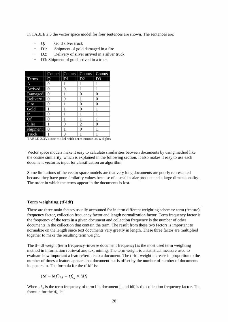
28
In TABLE 2.3 the vector space model for four sentences are shown. The sentences are:
- Q: Gold silver truck
- D1: Shipment of gold damaged in a fire
- D2: Delivery of silver arrived in a silver truck
- D3: Shipment of gold arrived in a truck
Counts Counts Counts Counts
Terms Q D1 D2 D3
A 0 1 1 1
Arrived 0 0 1 1
Damaged 0 1 0 0
Delivery 0 0 1 0
Fire 0 1 0 0
Gold 1 1 0 1
in 0 1 1 1
Of 0 1 1 1
Siler 1 0 2 0
shipment 0 1 0 1
Truck 1 0 1 1 TABLE 2.3Vector model with term counts as weights
Vector space models make it easy to calculate similarities between documents by using method like
the cosine similarity, which is explained in the following section. It also makes it easy to use each
document vector as input for classification an algorithm.
Some limitations of the vector space models are that very long documents are poorly represented
because they have poor similarity values because of a small scalar product and a large dimensionality.
The order in which the terms appear in the documents is lost.
Term weighting (tf-idf)
There are three main factors usually accounted for in term different weighting schemas: term (feature)
frequency factor, collection frequency factor and length normalization factor. Term frequency factor is
the frequency of the term in a given document and collection frequency is the number of other
documents in the collection that contain the term. The result from these two factors is important to
normalize on the length since text documents vary greatly in length. These three factor are multiplied
together to make the resulting term weight.
The tf–idf weight (term frequency–inverse document frequency) is the most used term weighting
method in information retrieval and text mining. The term weight is a statistical measure used to
evaluate how important a feature/term is to a document. The tf-idf weight increase in proportion to the
number of times a feature appears in a document but is offset by the number of number of documents
it appears in. The formula for the tf-idf is:
Where tfi,j is the term frequency of term i in document j, and idfi is the collection frequency factor. The
formula for the tfi,j is:

29
Where ni,j is the number of occurrences (term count) of the considered term ti in document dj, and
is the sum of all terms in document dj, or in other word, the size of document dj. The reason
why the term count is dividend on the length of the document is to normalize the document on the
length. If this were not done, the term weight would have a bias towards longer documents.
The inverse document frequency (idfi) is obtained by dividing the total number of documents by the
number of documents containing the term, and then taking the logarithm of that. It is a measure of the
general importance of the term. The formula for the idfi is as follows:
Where, |D| is the total number of documents in the collection and is the number of
document in which the term/feature ti appears. If the term ti does not exist in the collection it will lead
to a division by zero. It is therefore more common to use .
The higher tf-idf value a term gets, the more important it is. A high value is reached when the term
frequency in the given document is high and when there are few other documents in the collection
containing the given term/feature. This term weighting method tends therefore to filter out common
terms by giving them a very low value.
In the gray area in TABLE 2.4 we can see the tf-idf scores for the example sentences motioned in the
above section about the vector space model.
tfi TF-DF
Terms Q D1 D2 D3 idfi Q D1 D2 D3
A 0 0.1429 0.125 0.1429 0 0 0 0 0
Arrived 0 0 0.125 0.1429 0.1761 0 0 0.022 0.0252
Damaged 0 0.1429 0 0 0.4771 0 0.0682 0 0
Delivery 0 0 0.125 0 0.4771 0 0 0.0596 0
Fire 0 0.1429 0 0 0.4771 0 0.0682 0 0
Gold 0.3333 0.1429 0 0.1429 0.1761 0.0586 0.0252 0 0.0252
in 0 0.1429 0.125 0.1429 0 0 0 0 0
Of 0 0.1429 0.125 0.1429 0 0 0 0 0
Siler 0.3333 0 0.25 0 0.4771 0.1589 0 0.1193 0
shipment 0 0.1429 0 0.1429 0.1761 0 0.0252 0 0.0252
Truck 0.3333 0 0.125 0.1429 0.1761 0.0586 0 0.022 0.0252 TABLE 2.4: Vector model with tf-idf scores
Similarity measure (cosine similarity)
Cosine similarity is used to calculate the similarity between two vectors, document vectors in this
case. This is done by measuring the cosine of the angel between the two vectors. FIGURE 2.3 show
two document vectors, and it’s the angle between them that is measured. When the angle between the
two vectors are zero it means that they are identical, and the bigger that the angel between them is the
more dissimilar they are. The cosine is equal to one when the document vectors ere identical, and it
gets lower the more unlike each other they are. In text mining (and other fields working with text

30
documents, e.g. information retrieval) the cosine similarity between two documents will range from
zero to one, since the term frequencies cannot be negative, thus the angle between two term frequency
vectors cannot be greater than 90°. Cosine similarity is often used to compare documents in text
mining and in information retrieval. In addition, it is used to measure cohesion within clusters in the
field of Data Mining.
FIGURE 2.3: document vectors in vector space
The cosine formula is derived from the Euclidian dot product formula:
Given two document vectors, A and B, of feature weights, the cosine similarity, θ, is represented using
a dot product and magnitude as:
A reason why the cosine similarity is one of the most used similarity measures for text documents is
that it normalizes document length during comparison. This is very important when comparing text
documents since they varies greatly in length.
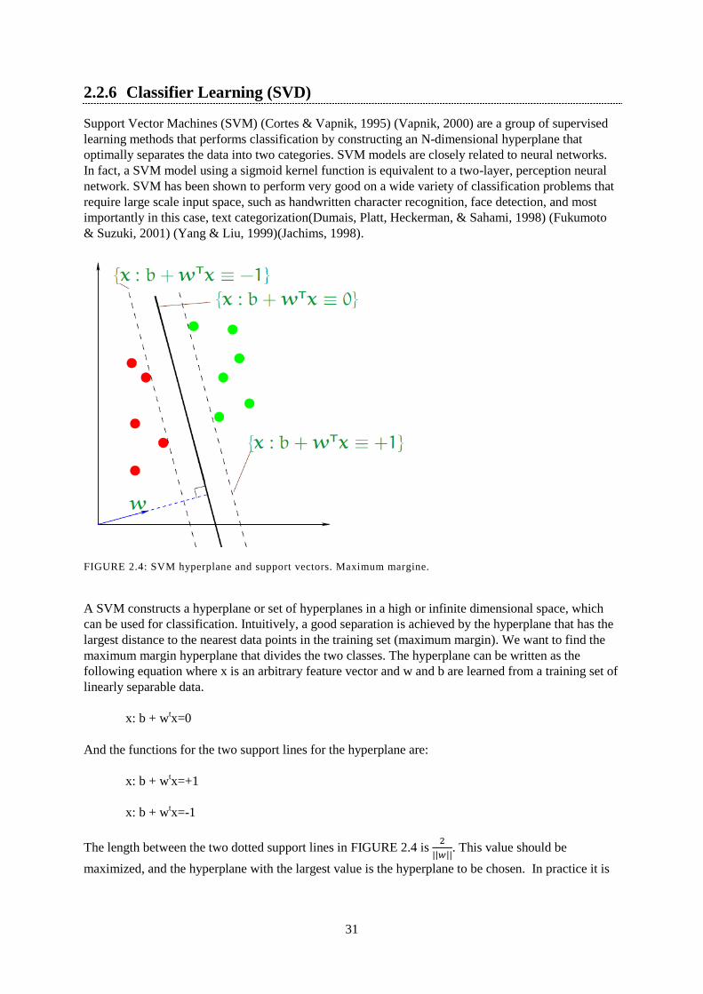
31
2.2.6 Classifier Learning (SVD)
Support Vector Machines (SVM) (Cortes & Vapnik, 1995) (Vapnik, 2000) are a group of supervised
learning methods that performs classification by constructing an N-dimensional hyperplane that
optimally separates the data into two categories. SVM models are closely related to neural networks.
In fact, a SVM model using a sigmoid kernel function is equivalent to a two-layer, perception neural
network. SVM has been shown to perform very good on a wide variety of classification problems that
require large scale input space, such as handwritten character recognition, face detection, and most
importantly in this case, text categorization(Dumais, Platt, Heckerman, & Sahami, 1998) (Fukumoto
& Suzuki, 2001) (Yang & Liu, 1999)(Jachims, 1998).
FIGURE 2.4: SVM hyperplane and support vectors. Maximum margine.
A SVM constructs a hyperplane or set of hyperplanes in a high or infinite dimensional space, which
can be used for classification. Intuitively, a good separation is achieved by the hyperplane that has the
largest distance to the nearest data points in the training set (maximum margin). We want to find the
maximum margin hyperplane that divides the two classes. The hyperplane can be written as the
following equation where x is an arbitrary feature vector and w and b are learned from a training set of
linearly separable data.
x: b + wtx=0
And the functions for the two support lines for the hyperplane are:
x: b + wtx=+1
x: b + wtx=-1
The length between the two dotted support lines in FIGURE 2.4 is
. This value should be
maximized, and the hyperplane with the largest value is the hyperplane to be chosen. In practice it is

32
much easier to minimize
instead of maximizing
. As we also have to prevent data points
from falling into the margin, we add the following constraint: for each data point:
b + wtxi >= +1 for xi of the first class
b + wtxi <= -1 for xi of the second class
This can be rewritten as:
Yi(b+wtxi)>=1 for all 1<=i<=n
Xi is a feature vector of the ith training document in a training set of n documents and yi is the class
label of the ith training document. All vectors lying on one side of the hyperplane should preferably
belong to one class while those on the other side should belong to another. If this is not the case then
the optimizing criteria has to be updated from only maximizing the distance between the support lines
to adding a penalty for miss-classifications.
To maximize the margin by the given constraint, the following function has to be minimized.
This is a quadric programming optimization problem, which is very time consuming. However, it can
be broken down into a series of smaller problem by a sequential minimal optimization algorithm
which is used for training SVMs.
FIGURE 2.5: SVM problem that is not linearly separable
When the problem is stated in a finite dimensional space, it often happens that in that space the sets to
be discriminated are not linearly separable, se FIGURE 2.5. This problem is difficult to solve when
x=(r,s) has only two dimensions. A solution to this is that the finite-dimensional space are mapped into
a much higher-dimensional space, this usually makes the separation easier. For the case in FIGURE
2.5 this could be done by mapping the function into this five dimensional function, T(X)={r,s,rs,r2,s
2}.
Doing this makes it possible to find a linear separator for that problem. SVM schemes use a mapping
into a larger space so that cross products may be computed easily in terms of the variables in the
original space. The cross products in the larger space are defined in terms of a kernel function K(xi,xj)
selected to suit the problem. A kernel is a similarity measure defined by an implicit mapping ø, from

33
the original space to a vector space such that: k(xi,xj)=ø(xi)Tø(xj). The choice of the kernel function is
very important for the efficiency of the support vector machine. Some common kernels are:
- Linear Kernel: k(xi,xj)=xitxj
- Polynomial kernel: k(xi,xj)=(gamma(xiTxj)+c)
d
- Radial basis function (RBF) kernel: k(xi,xj)=exp(-gamma||xi-xj||2)
- Sigmoid kernel: k(xi,xj)=tanh(gamma(xiTxj)+c)
2.2.7 Evaluation Metrics
In the context of classification tasks, the terms true positives (TP), true negatives (TN), false positives
(FP) and false negatives (FN) are used to compare the class labels assigned to documents by a
classifier with the classes the items actually belongs to. True positives (TP) are examples that the
classifier correctly labeled as belonging to the positive class. False positive (FP) are examples which
were not labeled by the classifier as belonging to the positive class but should have been. True
negative (TN) are examples that the classifier correctly labeled as belonging to the negative class. At
last there is false negative (FN) which are examples which were not labeled by the classifier as
belonging to the negative class but should have been. See TABLE 2.5, for a visual aid on how they
belong together. Other evaluation measures like precision, recall, F-measure, specificity and accuracy
can easily be calculated from these four variables.
Correct labels
Positive Negative
Classified labels Positive TP
(True positive)
FP
(False positive)
Negative FN
(False negative)
TN
(True negative) TABLE 2.5: Contingency table (TP, TN, FP, FN)
Accuracy
A common measure for classification performance is accuracy, or its complement error rate. Accuracy
is the proportion of correctly classified examples to the total number of examples, while error rate uses
incorrectly classified instead of correctly. In general, the better the classifier, the higher the accuracy
is. However, one should be careful to use only accuracy when one is using skewed data. This is
because when one class occurs significantly more than the other, the classifier might get higher
accuracy by just labeling all examples as the dominant class then what it gets when it tries to classify
some with the other class.

34
Precision and recall
Precision and recall are two widely used metrics for evaluating performance in text mining, and in
other text analysis field like information retrieval. They can be seen as extended versions of accuracy,
and by using a combination of these measures the problem with skewed data for classifiers dissipates.
Precision can be seen as a measure of exactness, whereas recall is a measure of completeness. In other
words, a high precision means that the most of the documents labeled as positive are labeled correctly
(but it might not have found many of the positive documents) and a high recall means that it has found
most of the positive documents (but it might also have labeled many negative documents as positive).
The higher the precision gets, the lower the recall becomes, and the higher the recall is the lower the
precision is.
Precision is the number of examples correctly labeled as positive divided on the total number that are
classified as positive, while recall is the number of examples correctly labeled as positive divided on
the total number of examples that truly are positive. This is shown in the following formulas.
F-Measure
F-Measure is the harmonic mean of precision and recall. This gives a score that is a balance between
precision and recall. Precision and recall captures two different, but important, aspects of the
classifiers performance, and the F-Measure combines them into one score for easier usage. In this
thesis the Fβ-measure is used because it can use its beta parameter to weight the importance of
precision and recall differently. This is important because it might be better to optimize the system to
favor either the precision or the recall if one of these has a more positive influence on the final result
of the trading simulation than the other.

35
3 Related Work on News-Stock Relationship
Systems
While there is a multitude of published articles about data mining, time series and other techniques in
prediction of stock prices, the numbers of articles covering the application of text mining in stock
market predictions are few. The reason for this is that this is still a new field. Some of the earlier
works that started to use textual news articles for financial forecasting is from 1998 (B, et al., 1998)
and 2000 (Lavrenko, Schmill, Lawrie, Ogilvie, Jensen, & Allan, 2000). The systems described in this
section is however of more recent dates.
3.1 Outline of Related Methods
The general structure of the earlier published related works has many similarities between them. All of
those reviewed in this thesis are build around a central learning algorithm (mostly a classifier) for
predicting the sentiment (price direction) of news articles. And for the learning algorithm to work it
needs a training set. The generating of those training sets is done in many different ways so they are
described in a separate section. A set of features has to be extracted from each news document for the
learning algorithm to be able to work on them. Different systems do this in different ways, and since
this is a vital part, it is described in its own section. At the end the architectural structure of these
different systems is described in more detail.
3.2 Training Set Creation
Most of the sentiment categorization methods involves a classifier that needs to be trained on a set of
pre sentiment labeled documents or with a vocabulary of sentiment labeled features (words) to be able
to correctly categories new news articles. Training sets can either be generated manually by experts
(Xun & Chen, 2005), or they can be generated automatically by the system. The automatic sentiment
categorization approaches are of most interest for this project since the manually based methods are
more time consuming and requires expert knowledge on the given domain to be sure that it is correct.
The NewsCATS engine (Mittermayer, 2004) categorizes news articles into a training set with these
three categories, “Good news”, Bad news”, and “No movers”. They categorize articles as “Good
news” if the stock price relevant to the given article has increased with a peek of at least +3% from its
original value at the publication time at some point during the 60 minutes that follows. The average
price level in this period has to be at least 1% above the price at publication. For “Bad news” the
opposite is true, the movements have to be in the negative direction instead. The rest of the articles in
between are classified as “No movers”.
The AZFinText system (Schumaker & Chen, 2010), is a regression system that tries to predict feature
prices and it is not a true sentiment classifier. This means that this system labels each news article with
a price value instead of sentiment label. The AZFinText system does this by labeling each news article
with the stock price 20 minutes after it is published.

36
The system developed by Pegah
Falinouss in his master thesis
(Falinouss, 2007) uses some time
series segmentation techniques to find
price trends by reducing the noise in
the price curve. FIGURE 3.1 shows a
segmented time series and how news
articles are linked to it by the time
they are published. He talks about two
different method of labeling the news
articles. Method one is “observed time
lag”, which has a time lag between
publishing time and when the public
absorbs and act on it. This means that
group X in FIGURE 3.1 is responsible
for trend B. he has used this kind of
labeling. The second method, which Falinouss has chosen to use, is build on the efficient market
theory, which state that there is no time lag between publishing time and market correction for this
piece of information. This means that news article group X in FIGURE 3.1 is responsible for trend A
and group Y for trend B.
The system created by Fook Hwa Tan in his master thesis (Tan) describes two labeling methods; (I)
labeling by trading volume and (II) labeling by returns. Labeling by using the volume labels news
articles into two classes, high volume and low volume. The division is controlled by whether the given
volume is above or below the average trading volume or above/below the average trading volume
plus/minus the standard deviation over the whole period. A classifier trained by this method can only
predict whether a news article will initiate a high number of trades or not, it cannot predict the
direction of the price movement. Labeling by returns looks for abnormal return amounts and label
news articles from that. Abnormal is the actual return minus the expected return, which is calculated in
the following manner:
Abnormal return = actual return – ( α+ β* return on the market index )
Actual return = return from the given stock
Return on the market index = Return from the entire stock market
Where α show how much on average the stock price changed when the market index was unchanged,
and β tells us how much extra the asset price moved for each 1 percent change in the market index.
The abnormal return values is then used to label news articles as rise, plunge or not relevant. A
parameter called gamma is used to control how far above or below zero the abnormal return has to be
for the news article to be labeled as rise or plunge and not as not relevant. Tan uses a one day interval
to calculate the return values (selling price – buying price) for finding the abnormal returns value.
However, he chose this interval because he did not have access to intraday data, and he refers to
studies stating that shorter intraday intervals give better results.
FIGURE 3.1: Trend, news alignment methods

37
3.3 Document Representation
The vector space model together with the tf-idf feature weighting method (see section 2.2.5) is the
most common approach among the different systems for representing the news articles. However there
are many different methods for extracting and selecting the features used in these vector space models.
The NewsCAT engine (Mittermayer, 2004) is one of the methods which use a vector space model with
a tf-idf feature weighting scheme. It uses single words, or unigrams as features, but it only selects n
features with the highest tf-idf score to represent the news article.
Schumaker and Chen (Schumaker & Chen, 2006) examined the role of financial news articles on three
different textual representations; Bag of Words, Noun Phrases, and Named Entities and their ability to
predict discrete number stock prices twenty minutes after an article release, which is a regression
problem and not a categorization problem. They demonstrate that using a Named Entities
representation scheme performs better than the de facto standard of Bag of Words on their Support
Vector Regression (SVR) prediction engine.
Bag of Words Noun Phrases Name Enteties
Fined Reuters Reuters
Fourth quarter NYSE Fourth quarter
The NYSE Fourth quarter Schwab
Schwab Profit
Profit Schwab
fell
TABLE 3.1 Feature types from (Schumaker & Chen, 2006)
The bag of words technique is the standard way of representing a text document and it is simply a
collection of the words believed to best represent the document. Noun phrases (NP) is a phrase
normally consisting of a head noun, which is often together with a modifier set (e.g. the red ball, or a
ball). Name entities (NE) are words and phrases describing things like names of persons,
organizations, locations, expressions of times, quantities, monetary values, percentages, etc. Name
entities are a more specific and concrete form of noun phrases. Some examples of features extracted
from a text by these three different methods can be seen in TABLE 3.1.
The trading method invested $1,000 per new trade, and TABLE 3.2 shows how much each of the
different trading methods gave in return after a fixed trading period. Noun phrases gave the biggest
return from the simulated trading run with a return of $6,353, next was bags of word with $5,111 and
Simulated trading Regression Model
Bag of Words -$1,809 $5,111
Noun Phrases -$1,809 $6,353
Name Enteties -$1,879 $3,893
TABLE 3.2: Return from Simulated trading (Schumaker & Chen, 2006)
Outlay Model
Bag of Words $228,000
Noun Phrases $295,000
Name Enteties $108,000
Percentage return Model
Bag of Words 2.24%
Noun Phrases 2.15%
Name Enteties 3.60% TABLE 3.3: Percentage return on money invested
(Schumaker & Chen, 2006) TABLE 3.4: Money invested
(Schumaker & Chen, 2006)

38
name entities had the lowest return with $3,893. However, TABLE 3.4 shows that noun phrases and
bags of words invested much more money in total, which means they performed many more trades
since each trade only invested $1,000. If the amount of money invested is taken into consideration it
shows that the name entities method gives a much higher percentage return on the money invested
than what the two other methods does, this can be seen in TABLE 3.3. This means that the two other
methods predicted wrong many times more than what the name entity method did.
The AZFinText model (Schumaker & Chen, 2010) extracts proper nouns and selects the proper nouns
that occurs three or more times to be used as features. They are the same people that did the above
study where they concluded that of the three feature types; bag of words, noun phrases and name
entities, the name entity feature type gave the best results. However in this system they chose to use
proper nouns (not included in their previous study), which is a subset of the set of noun phrases and a
super set of the name entity set, which means it lies in between those two sets.
3.4 Architectures of News Based Trade Support Systems
This section describes the system architecture and shows some of the results of a few different
systems. Parts of them are described in the above sections. Most of them, in addition to analyzing
news articles, also have added a trading engine and shows the result from some simulated trades.
3.4.1 NewsCAT
The NewsCAT method (Mittermayer, 2004) tries to predict price trends (incline, decline or flat)
immediately after press release publications. This system consists mainly of three components, and
how they are connected in a system can be seen in FIGURE 3.2: NewsCATarchitecture. The sentiment
labeling news articles that are used as a training set for train the NewsCAT classifier is described in a
paragraph under section 3.2.
Text preprocessing engine: This component retrieves relevant information from press
releases and transfers them through a preprocessing stage
consisting of tokenization, stop-word removal and stemming.
Features are then selected from the n number of words with
the highest tf-idf score.
News Categorization engine: This component sorts each press releases into predefined
categories, “Good News”, “Bad News” or “No Movers”.
NewsCAT uses support vector machine (SVM) as its
classification algorithm.
Trading strategy engine: This component derives appropriate trading strategies for
when to buy, sell and hold by the use of the output from the
categorization engine.

39
FIGURE 3.2: NewsCATarchitecture
FIGURE 3.3: NewsCAT vs random - trade profit
The selection of no movers by the NewsCAT system is reported to be fairly good, while the selection
of “good news” and “bad news” is fairly bad. They believe the reason for this is that the words used in
“no movers” documents and for “movers” documents probably are very different while the words in
“good news” and “bad news” documents might be more similar (e.g. only the word “not” might spate
a good and a bad article in some cases). The system is reported to significantly outperform a trader
randomly buying and shorting stocks immediately after press releases, which can be seen in FIGURE
3.3: NewsCAT vs random - trade profit. Ass seen the system has an average profit of 0.11% per trade
while the random trader has zero profit. By using a different trading strategy which used some support
lines as barriers to lessen some of the risk they managed to get a 0.21% profit per trade while the
random trader only got 0.07% with the same strategy.

40
3.4.2 AZFinText
The Arizona Financial Text System (AZFinText) (Schumaker & Chen, 2010) is another machine
learning system that uses financial news articles and stock quotes as its input to predict feature stock
price movements. As mentioned earlier in section 3.3, this system uses proper nouns as features, and
selects the proper nouns that occurs three or more times to be included in the feature set. It
distinguishes itself by using a support vector regression (SVR) algorithm instead of a classification
method as most of the other system are using. This means that it tries to predict a feature price value
when given an article; more precisely it uses the article to predict what the price will be in 20 minutes.
While the other methods mentioned in this thesis only categorizing the news as good, bad or neutral.
AZFinText have implemented a trading engine that buy or short a stock if the predicted price
movement is greater or equal to 1%, and any stock bought or shorted are then liquidated after 20
minutes. FIGURE 3.4: AZFinText architecture illustrates how the AZFinText system is designed.
FIGURE 3.4: AZFinText architecture
The AZFinText system was tested on S&P 500 and compared against the top quantitative funds32
. It
had an 8.5% return in the given period, while the S&P 500 had a lesser return of 5.62%. It ranked as
number four against all the other quant funds. However, those quant funds that ranked above it traded
in different markets than the AZFinText system. When ranked against other quant funds trading only
in S&P 500 then AZFinText system performed better than the rest of them, as seen in TABLE 3.5.
Return
AZFinText 8,50%
Vanguard Growth & Income (VQNPX) 6.44%
BlackRock Investment Trust Portfolio Inv A (CEIAX) 5.48%
RiverSource Disciplined Equity Found (ALEIX) 4.69%
TABLE 3.5 AZFinText vs quant founds
The AZfinText system has also been used together with two basic quantitative portfolio selection
strategies in an attempt to increase the performance of the system. The two quantitative portfolio
selection techniques used was a Momentum strategy and a Contrarian strategy. The hybrid system
with the use of the Momentum strategy with a 1-week portfolio formation period archived 20.79% in
trading return, which is much better than the 8.50% that the AZFinText system had alone. In
32
A quantitative fund or quant is an investment fund in which investment decisions are determined by numerical
methods rather than by human judgment. (Dempester, Gautam, & Pflug)(Quantitative fund: Wikipedia)

41
combination with the Contrarian strategy over a five-week holding period, the system had a 4.54%
trading return.
3.4.3 Falinouss
The main parts of the system developed by Pegah Falinouss in his master thesis (Falinouss, 2007) can
be seen in figure x. These steps consists of finding price trends by time series segmentation, then each
news document are sentiment labeled by aligning them up with the price trend. The document
preprocessing part consists of the three standard methods; tokenizing, stop-word removal and
stemming. Then the documents for the training set are selected by going thru a process called
document selection. This process calculates the chi-square value for each feature and only selects
documents with minimum one significant feature. After that the document representation is done by
the standard method of using a vector space model with tf-idf as the term weighting method. This
system also includes a feature reduction process which is done by the random projection (Bingham &
Mannila, 2001) method. And at last the SVM classifier is used for classifying the sentiment of news
articles as rise or drop.
This system is reported by Falinouss to have an accuracy of 83% for correctly labeling a news article
as rise or drop. The recall of rise predictions are stated to be 67%, and for drop predictions it is 93%.
The precision for rise predictions are claimed to be 87% and for drop 81%. Falinouss did not include
an evaluation part on how good this system is when used for trading stocks.

42
4 Scientific Approach
In the previous chapters a variety of methods used for news based trading systems have been
reviewed. Based on this theory, an automatic news based trading decision support system was
developed. This chapter provides a description of the implemented system.
4.1 Approach Overview
The approach adopted in this thesis is based on classification of published news articles as being
positive, neutral or negative. If a news article is positive it means that it is likely to be followed by an
upward moving price trend for the specific stock, if it is neutral the price trend is likely to be flat, and
if negative the price trend is likely to fall. Then a trading decision maker uses this information about
the news article to make a trading decision regarding the stocks of the related company.
The implemented system consists of a number of main concepts. First, the time stamped news articles
and stock prices needs to be acquired from internet during a data acquisition process. Then these news
articles have to be labeled so they can be used in training and testing the classifier. This entire process
is shown in FIGURE 4.1. The top part of the figure shows the component involved in data acquisition,
which is described in detail in section 4.2. Next it is the news labeling component which labels news
automatically by using stock prices, it is described in section 4.3. The next component in FIGURE 4.1
is the document preparation process, which is described in section 4.4. In it, each news article goes
through a process that consists of a document preprocessing part, a document elimination part, and a
document representation part. Then the documents are entered into a label refining process in an
attempt to improve the correctness of their labels; this component is described in section 4.5. The
labeled news articles are then used for training and testing of the classifier. The last component in the
figure is the trading process, it takes news articles labeled by the trained classifier as input and
simulates stock trades based on what type of label it is. The classifier and the trade engine are
described in section 4.6 and 4.7. Not all the steps in FIGURE 4.1 are required. Some are optional and
others have multiple choices. Some of the optional ones are stop-word removal and stemming, and
some of those with multiple choices are label refining and feature reduction.
The programming language Python was used to do all the programming for this system. Some
packages (libraries) were used for the development, the main ones being natural language toolkit
(NLTK) and SVMLIB with its Python interface.

43
FIGURE 4.1: The workflow of our proposed automatic news based trading approach
4.2 Data Acquisition
For this project two types of data are required; (I) time stamped news articles and (II) stock prices.
This data acquisition step is performed at the beginning, and can be seen in FIGURE 4.1. The
following sections describe how these two types of data are gathered.
4.2.1 Collection of News Articles
The news articles that are gathered will be labeled as positive, neutral or negative. The labeling
techniques that are used to label the news articles are doing it by using stock prices. This means that
the news articles that are to be gathered must be time stamped so they can be linked to stock prices.
The web page Netfonds gathers time stamped news articles from various financial news sites and

44
groups them together according to the companies they belong to. This means that in addition to
fulfilling the requirement of having time stamped news articles, this site also removes the need to
make a categorization engine to group news articles together with companies they belong to. Three of
the financial news sites that Netfonds collect news from are; Hegnar online, Newsweb, and Thomson
Reuters ONE.
A web crawler is created which takes a starting date, days to look back, and one or multiple tickers as
parameters. Then it crawls the site to look for news articles fitting these parameters. Each news article
is stored in a text file under the folder named after the company it belongs to. The naming convention
of the text file is like this: “date time company-ticker news-source title.txt”. The news articles
information is stored inside the text file with additional information and in a structured way that makes
it easier to be reused later on:
<doc>
<date></date>
<time></time>
<source_link></source_link>
<source></source>
<text>
<title></title>
<body></body>
</text>
</doc>
Some of the news sources publish articles in both Norwegian and English without giving any kind of
identifier to separate the two languages. This raised the need to create a language classifier. Since this
would only be used to separate two languages this is done by creating a set of high frequency words
for each language and labels each news article with the language it had most words in common with.
This process is a part of the news article collection component FIGURE 4.1; it is not shown in the
figure.
4.2.2 Collection of Stock Quotes
Stock prices are collected about companies in Oslo Stock Exchange (OSE), and both intraday and
daily stock quotes are gathered. Intraday trade information was provided by one of the project
supervisors, Arvid Holme. A program is also written for gathering daily quotes from the web page
Netfonds, which has daily quotes as far back as 2001 on some companies. Intraday quotes consists of
date, time, price and volume information for each trade, while daily quotes consists of date, time, open
price, high, price low price, close price, and trading volume for that day.

45
4.3 News Sentiment Labeling by Price Trends
This method creates a training set of news articles for the news sentiment classifier by automatically
labeling each news article with a sentiment. This is done by looking at how the price trends move after
the news articles are published. If the price trend is up, then the news is labeled as positive, if the trend
is down, then it is negative, and when the trend is flat it is labeled as neutral. This can be done on both
intraday and daily prices. A couple of different methods to do this labeling are developed, but the main
idea behind each is the same. After this process is finished, each news article is labeled as positive
(uptrend), neutral (flat), or negative (downtrend). This step, as seen in FIGURE 4.1, is done after the
data acquisition step and before the document preparation. The reason why this step is performed
before any news article documents are prepared is that this step only needs the news article id,
publication date and time, and stock prices, and not the content of the news.
4.3.1 News Trend Labeling: Method One
The first method is similar to the method used by NewsCAT (Mittermayer, 2004). It finds the average
price for a given period following directly after the publication of the news article, If this value has
changed more than a given percentage α from the price at publication, and if a maximum price in the
price trend direction has been above a given percentage β than the start value, then the article is
classified as either positive or negative based on the direction of the price trend after publication. If
this is not the case, then it classified as neutral. This process is shown in FIGURE 4.2, and can be
easier to understand by looking at the following algorithm.
FIGURE 4.2: News labeling from price trends method one - from NewsCAT

46
4.3.2 News Trend Labeling: Method Two
The second method finds the straight line that best fits the price values in a given period after the
publication by using the least square method. It then calculates the slope of this line, and if it is larger
than a given threshold value the news article is classified as positive or negative, depending on the
direction of the slope. If the slope does not cross this threshold value, then it is classified as neutral.
This method has been used only in the very early experiments, and is not used in the experiments
performed in chapter 6. The slope for the regression line is found according to the following formula:
FIGURE 4.3: NEWS LABELING FROM PRICE THRENDS METHOD Two
4.3.3 Combining different labeled data sets
One method that might increase the correctness of the labeled data set is to combine two different data
sets labeled by the first or the second methods to a single set. The two training sets are generated with
different parameter setting, and one should use a longer trend duration while the other should use a
shorter one. This will ensure that the two data sets are not identical. The new data set should consist
only of documents that are labeled with the same sentiment in both of the other sets. This reduces the
total number of documents in the data set, but the sentiment label should, in theory, be more likely to
be correct.
4.3.4 Price trend timing
As mentioned above, labeling is done by using the price trend after the article is published. Most of the
related research that uses an automatically labeled training set uses stock price trends in their labeling
techniques. However, how to decide when this trend starts in relation to the time the news article is
publishes varies greatly between the different approaches. The start points of the trend is, as seen later
in the experiments in chapter 6, important for the labeling method to produce more correct labels, at

47
least when daily prices are used. The reason for this is that daily price data only operates with two
timed values, opening and closing prices. This means that the price trend might have been started long
before or after the time the news article was published. This means that the market might already have
adjusted to the news before the trend calculation started if it is started after the news is published. If it
is started before, it might be that the trend is in response to some other piece of information and not
the given news article. Of course, this last problem is also likely to give some false labels when there
is multiple news articles published in one day for a given company, which is often the case for the
more popular companies. The methods described in label refining in section 4.5 will hopefully reduce
the impact of this problem thereby removing some of the noise in training sets that comes from it.
The price trends belonging to each news article are found in two slightly different ways when daily
prices are used. The only difference between the two methods is when they start to calculate the trend.
They give quite different outcomes, as seen later in the experiment one; hence it is important to choose
the right one.
Method one: It starts the trend from the price right before the article is published. This means that
the articles published before the stock exchange has opened starts its trend calculation
from the previous day’s closing price. Articles that are published during the opening
time starts with the opening price of that day and articles published after it has closed
start with that day`s closing price.
Method two: This method starts with the price immediately after the publishing time. That means
that articles published before the stock exchange open starts its trend calculation from
this day`s opening price. Articles that are published during the opening time starts with
the closing price of that day and articles published after it has closed start with the next
day`s opening price.
When labeling is done with daily price data only, the news articles published on trading days are used,
the rest of them are excluded. This is also true when labeling is done with intraday prices. However,
when intraday prices are used, then all news articles published outside of the stock exchange`s opening
time, or to close to the end of the opening time to calculate a price trend, is also removed. Intraday
labeling follows the general idea of method two for trend timing; however, it looks only at the
publication day and not over multiple days.
4.3.5 Manually Labeled Set
A collection of manually sentiment labeled documents is created. These labels are not decided by a
financial expert, so there might be some small errors in them. However, many news articles have a
clear positive or negative spin to them that non experts can identify. This manually labeled set of news
document set is primarily going to be used for evaluation, but it can also be used as seeds to create a
training set with a seed based approach, which are a semi-unsupervised clustering method. However,
this is not done in this thesis.
The manual labeling is done purely by reading some news articles and labeling. No stock price data is
taken into consideration when labeling, only the information given in the news article.
The manually labeled training set consists only of positive and negative documents. This means that
when the automatically created sets are compared with the manually labeled, they are only evaluation
how similar the positive and negative documents found by the automatic method are to the manual set.
The documents that are labeled as neutral are not evaluated.

48
4.4 Preparation of Data Set
After the news articles have been gathered they have to be prepared before they can be categorized.
This process can be seen in FIGURE 4.1. The steps in this process are; (I) document preprocessing,
(II) Features extraction and selection, (III) document elimination and (IV) document representation.
The prepared data sets will be used for training and testing of the classifier.
4.4.1 Document Preprocessing
The document preprocessing step consists of the four steps, tokenization, short document removal,
stemming, and stop word removal. Some of them are described in section 2.2.1. These steps can also
be seen in FIGURE 4.1 under document preprocessing.
Tokenizing: is done by first processing the text with the wordpunct tokenizer in the python
library “Natural Language Toolkit” (nltk), which is one of several tokenizers
in that particular library. It works by dividing the text into tokens by
separating it on whitespaces and on signs like comma, punctuation and
explanation signs. After that all signs are removed so only words and numbers
are left as tokens.
Short doc removal: The short document removal process removes short documents, just as the
name indicates. The minimum length of the remaining documents is given by
an input parameter for this function. This documents that are to short are
removed.
Stop-word removal: Method one for stop-word removal method one uses a Norwegian stop-word
list which is inside the nltk package, but this list include some potentially
important words like “ned” (down) and “opp” (up), so a second method is
added which only removes words of two characters or less. This last method is
used on the experiments done on the final system.
Stemming: The stemming process uses a snowball based stemmer for the Norwegian
language, which is also included in the nltk package.
4.4.2 Features
At this stage the news documents has been preprocessed and is now ready for the feature extraction
process. These features that are extracted are later used when the documents are represented. This
stage also has a feature elimination step to remove some features that are likely to be of little
importance.
Feature Extraction
This process extract features from the news documents. Two types of features can be extracted;
unigrams and bigrams. These feature types are described in greater detail in section 2.2.2. These two
feature types are compared against each other in section 5.5, and bigrams are chosen to be used for the
experiments in chapter 6. The features that are extracted are placed in an inverted index.

49
Feature 1 {(doc id, frequency, term weight), (doc id, frequency, term weight)}
Feature 2 {(doc id, frequency, term weight)}
At this point only doc id and frequency is added. The term weight is added later in the document
representation part. The news articles are now on good way to their finished representation. However,
the last steps in this process come later under the document representation part.
Feature Elimination
This part simply eliminates features that occur in less than a given number of documents. The reason
why these features are removed is that they are very unlikely to be of any help for classifying since
they occur so seldom.
4.4.3 Document Elimination
After each news article has been labeled we need to eliminate documents that are not at any use for the
classifier. Not every document is useful for prediction, in reality many documents are useless for this
purpose and thus only contributes as noise. Only documents that contains at least one significant
feature for distinguishing between the three categories; positive, neutral and negative are kept. Those
documents that do not include any significant features are removed because they are of no use for
training the classifier. The feature selection method chosen in this thesis is the chi-square method, se
section 2.2.2 for explanation.
4.4.4 Document Representation
The vector space model is used as document representation. More general information on document
representation can be found in section 2.2.5. Each document is represented by a vector of numeric
values where each value indicates the importance of the feature connected to it. These values are
calculated by the chosen term weighting method, which in this case is the tf-idf method (see section
2.2.5 for explanation). When the document representation vector is created, features that are not in the
given document will be given value zero. This means that each document vector has the same n-
dimensions, where n is the number of selected features.
Term weighting: The feature weighting method that is chosen is the popular tf-
idf method, which is described in section 2.2.5. The tf-idf
method is very popular and generally gives good results while
still being quite efficient.
Dimensionality reduction: The SVD method, which is described in section 2.2.4, is
chosen to perform the feature reduction. The SVD method is
well known and gives good results, but it is slow and demands
huge amounts of memory. This is not a problem for this thesis,
but for a real time news-trading assistant product, another
faster and less memory demanding approach is better suited
(e.g. random indexing). A second feature reduction technique
is also implemented. It simply find the chi-square values for
each feature and either pick top n features or pick all features
with a value above a given threshold value. This method
might more correctly be named feature selection and not
feature reduction. The SVD method is used in most of the
experiments.

50
4.5 Label refining
After each news article is sentiment labeled by the basic method of using price trend directions, and
after all the documents have been prepared and given a document representation, a label refining step
is added in an attempt to improve the labels given to the news articles. The reason why this is done is
that the basic labeling method is very likely to result in a labeled data set with a significant degree of
noise. If daily price data is used, then all articles published in the same day is given the same
sentiment, but some of them are likely to be neutral, if not the opposite sentiment. It still will be noise,
even when intraday price data is used because the news article sentiment will not always correlate with
the same price trend.
The documents given to this method is labeled by the basic labeling method with positive, neutral, or
negative labels. If we assume that a document with a given label has more in common with other
documents of the same labels than it has with documents with different labels. And we assume that the
basic labeling method gives more correctly labeled news articles than falsely labeled ones. Then one
possible way to fix this noise problem is to use some kind of clustering method to rearrange the
documents in these three groups of labeled documents. This should work if the assumptions are correct
because then the three groups of positive, neutral and negative documents is in fact three clusters.
By adding this technique of label refining the classifier performance should be better when it is tested
on the automatically labeled training set. This is because the three groups has become easier to
distinguish because of the clustering process, thus it becomes easier to train a good classifier.
However, the labels might still be noisy with many incorrect labeled news articles. The reason for this
is that not every document that is close to a group of documents with one label is necessarily of the
same label as them. However, the clustering methods will give them the same label as its closest
neighbors, even if that is an incorrect label.
4.5.1 K-Means clustering
The k-means algorithm is one of the simplest unsupervised learning algorithms that are used for
clustering documents, or data. It clusters the data in k clusters, and it does it by executing the
following steps.
K-Means algorithm:
1. Place K points into the space represented by the objects that are being clustered. These points
represent initial group centroids.
2. Assign each object to the group that has the closest centroid.
3. When all objects have been assigned, recalculate the positions of the K centroids.
4. Repeat Steps 2 and 3 until the centroids no longer move. This produces a separation of the
objects into groups from which the metric to be minimized can be calculated.
In this problem, where the sentiment labels found by labeling the news articles from the price trend
direction have to improve, the initial k centroids are from the three groups of documents that are
labeled as positive, neutral, and negative. The closeness in step two is measured by the cosine
similarity between the documents and the cluster centroids, which are described in chapter 2.2.5.
This method is very likely to be clustering the document labels to much, thus it will likely have a high
noise factor because of many incorrectly labeled news documents. This means that the classifier
should perform very well when tested on the automatically generated data set, but it is not very likely

51
to perform that good when it is compared with the manually labeled data set. Because of this, a couple
of other method based on K-Means, but with some restrictions where implemented.
4.5.2 Restricted k-Means clustering method one
A refining method based on the K-Means clustering algorithm used above only with some added
restrictions is also created. These restrictions deny the clustering method to directly move documents
from positive to negative, and vice versa. If a document is told to do one of these moves, then it is
instead moved to the neutral cluster. However, the next clustering round, when the cluster centroids
has been updated, it is allowed to be moved to any location since there are no restrictions when
moving from the neutral cluster. The extra rules are like this:
1. Document from positive to negative: Not allowed, move to neutral.
2. Document from negative to positive: Not allowed, move to neutral
3. Document from negative or positive to neutral: Allowed, move document to neutral
4. Document from neutral to any other cluster: Allowed, move document
5. Document from cluster x to cluster x: Allowed, keep document at same position
By adding these extra rules there are less documents that are moved from positive to negative and
negative to positive. This means that there should be less chance that the documents in the positive and
the negative clusters changes so much that these clusters no longer represents positive and negative
documents.
4.5.3 Restricted k-Means clustering method two
A second restricted method that is also based on the K-Means algorithm is also added. These
restrictions deny the clustering method to move documents from positive to negative, and vice versa.
If a document is told to do one of these moves, then it is instead dropped from the document
collection.
6. Document from positive to negative: Not allowed, remove document.
7. Document from negative to positive: Not allowed, remove document
8. Document from negative or positive to neutral: Allowed, move document to neutral
9. Document from cluster x to cluster x: Allowed, keep document at same position
This method will in most circumstances end up with a smaller news collection after it has finished
than it had before it began. However, it should lessen the likelihood even more that clusters rearrange
so much that they no longer represent positive, neutral and negative news documents, which might be
able to happen with the above method.
4.6 Classifier Learning
The classifier method used for the learning algorithm is the Support Vector Machine classifier (SVM).
It is used to find the sentiments of any given news articles, or more precisely, the relationship between
the contents of news stories and price trends. The LIBSVM library together with the included python
interface is used for implementation of the SVM algorithm. Among the possible kernels for the SVM
classifier (discussed in section 2.2.6), the RBF kernel which have proven to be best suited for text
classification is chosen. To be precise, the RBF kernel and the polynomial kernel have both proven to
perform best in different studier. However the RBF kernel is faster, and is therefore chosen instead of
the polynomial kernel. The RBF kernel requires two parameters to be set, cost and gamma. The details
on how these two parameters are chosen are described in section 5.6.

52
After each document has undergone the steps required to produce their document representation and
been labeled with a sentiment label they are randomly divided into two sets, a training set and a test
set. Typically the division is; 70 percent of the documents in the training set and the remaining 30
percent in the test set. The training set is used to train the classifier, while the test set together with a
manually labeled set are used to evaluate the performance of the system.
4.7 Trading Engine
The trading engine implements a straight forward and simple trading strategy, it is told by a decision
method whether to buy, sell (short selling) or do nothing. Then after a fixed duration of time it
liquidates the assets it bought or shorted. This is not a good strategy since the assets that are obtained
can experience huge losses and still nothing is done about it until the fixed time duration is finished.
However, this is not that important in this study because this weakness is the same for both the news
article based trader and the random walk trader, and it`s the comparison between them that`s of
interest. If one of them gives better results than the other with this method then it stands to reason that
it also performs better when companied by a better trading strategy.
There are three different decision methods for deciding what signal, buy, sell or hold, that are used by
the trade engine. These three methods are:
News article trading: This method decides its trading signal by analyzing news articles and
deciding what to do from the result of the analysis.
Random trading: This is basically a random trader. Buy, sell and hold signals are
randomly generated. The profit from this should overtime be on
average zero, but it is still implemented since it is easily done.
Buy and hold: This is method only buys and then holds the stock. In this setting it
means that the trade engine always is given a buy signal, and then
after the fixed time duration it sells what it has bought.
For simplification purposes the trading engine assumes that each trade is done with the same amount
of money, it therefore returns a percentage value to show how much it has returned. In this way it is
possible to just multiply it with the chosen amount of money to be used on each trade to find how
much it earns or losses. This is not the most realistic way of doing it since each trade seldom consists
of the same amount of money, but it gives a good indication of how the trading strategy does and for
the purpose of this article it is more than good enough.

53
5 Experiment Preparation
Before the main experiments can be performed some system parameters has to be chosen. This chapter
describes the parameter setting and why some of them were chosen. It also describes other
preparations like how the training and test sets are divided and from which companies they are created.
How the evaluation of the system is performed is also described in this chapter.
5.1 Evaluation methods
The purpose of this section is to describe the evaluation methods used for the experiments presented in
chapter 6. The evaluations of the training sets and the classifier are mainly performed with the
precision, recall and the F-Measure, while the evaluation of the trading engine are mainly done by
looking at the average percentage return per trade.
5.1.1 Direct comparison of Manually Labeled Set with Automatically
Generated Sets
One of the tests that are performed is to directly compare the manually labeled set with the
automatically labeled sets. This is done by comparing the positive documents in the automatically
labeled sets with the positive documents in the manually labeled and the negative documents in one
with the negative documents in the other. Precision and recall are used to find the F-Measure for the
positive and negative documents in the automatically labeled sets. Precision for positive documents
are found by dividing the number of correctly labeled positive (true positive) documents with all
documents labeled as positive (some negative and neutral document might be wrongly labeled as
positive). Recall for positive documents is found by dividing the number of correctly labeled positive
documents on all the documents that should have been labeled as positive. Precision and recall for
negative documents are found in the same way, only difference being that negative documents are
used instead of positive. Then the combined precision and recall for positive and negative documents
are calculated. The F-Measure used as an indicator of how similar the manually labeled set is with the
automatically labeled set are then calculated from the combined precision and recall scores.
5.1.2 Classifier Evaluation
Classifier evaluation is done in two ways. One is to evaluate it with a test set from the automatically
labeled set, and the other is to evaluate it with the manually labeled set. Both methods are done the
same way. They compare the predicted labels given by the classifier with the labels in the test set that
are labeled automatically and the labels in the manually labeled set. The comparison is done the same
way as in the above section. The precision and recall is found for the positive and the negative
documents, then they are combined and a F-Measure is found from this combined values.
5.1.3 Evaluation of Simulated Stock Trading
When evaluating the news based trading engine it should be compared with a random walk based
trader, and it should perform better for it to be of any value. This means that it should on average have
positive returns (profit) on its trades. This is however not enough, it should also be compared with the
“buy and hold” strategy, and it should preferably also outperform this one.

54
Some important values are the return, percentage gain or loss, for each trade with these strategies, the
number of trades each of them has performed, and also the maximum possible return to get on these
trades is of interest. Some useful statistic for comparison found by these values average return on each
trade for each of the strategies, and the portion of the maximum possible return they have managed to
get. All these values are the average of multiple training sets.
5.2 Document Preprocessing and labeling
The preprocessing step includes stop-word removal and stemming. It removes documents with less
than 25 features, short news articles are removed. All features that occur in less than 5 documents are
removed from the feature vocabulary. The data sets used in the experiments are created by the labeling
method one, which are described in section 4.3.1. The results shown in the experiment chapter shows
the average score of multiple different training sets. The training sets are created by looking at price
data from only one day into the future and all the way up to five days.
5.3 Training and Test Sets
To get a correct analysis of how the system works it is important to divide the prepared documents
into separate training and testing sets. The number of document in each labeled data set in usually
somewhere between 2000 and 2600 (never more than 2600) depending on how many is removed by
the document elimination process. The classifier evaluation simply divides the prepared documents
into two sets. Typically 70% of the documents are given to the training set while the remaining 30%
are given to the testing set, which is also how they are divided in this thesis. This is mostly how it is
done for the training and test sets for the trading engine too. However there is one exception when the
refining method two (see section 4.5.3) is used. This is because it removes documents to make the
clusters better. Those documents that it removes are added back to the test set (not to the training set).
If they were not added back the result would not be realistic since this process can’t be replicated if
news articles not included in the prepared data set were to be tested. This means that results from the
classifier evaluation of refining method two is probably a little better than what it is in reality if new
unlabeled documents were to be classified by it. If they however were to be added for the classifier
testing, the result would be worse than they truly are because the removed documents are very likely
to wrongly labeled. The reason why they are likely to be wrongly labeled is that label refining method
two removed them instead of moving them to a different cluster, thus they are still labeled with their
original label and not relabeled with a different label.
5.4 Training Set Sources: Multiple Companies
All the experiments performed on the system developed in this thesis are done with data sets created
from multiple companies from the same field. The classifiers are also trained on these training sets
created from multiple companies. This means that one classifier classifies news stories for multiple
companies after it is trained.
The reason why this is done is to obtain a larger data set. Few of the companies have enough news
stories published about them to get a data set of acceptable size. The classification results from these
sets are a little worse than data sets created from a single company that has enough news published
about it. FIGURE 5.1 shows that a training set created only by news articles about Statoil (STL)
performs much better than training sets created by multiple companies. However, when another

55
company than Statoil was chosen, a company with much less published news articles, then the results
would be much worse. This means that companies about which too few news articles are published
still can get a classifier to classify its news articles if that classifier was trained on news articles from
the same field as that company.
FIGURE 5.1: Comparison of training sets with multiple and single companies ( single = Statoil)
FIGURE 5.1 Shows how a classifier trained with a training set generated from multiple companies
(data set labeling method one is used with α=0.01 and β=0.02) compares against a classifier trained
with a training set generated from only one company(company is Statoil, and parameters are α=0.01
and β=0.02). As seen in the figure, there is only 0.04 points difference between the F-Measure of the
two methods.
By going for this larger data set the result is probably somewhat worse, but they should yield much
more steady results than what a smaller data set would. The companies that are chosen to create a
labeled data set are all companies from the oil business. That they all are in the same field should
lessen the penalty of using multiple companies somewhat. The companies used in creating the data
sets are “BW Offshore Limited” (BWO), “DNO International” (DNO), “Frontline” (FRO), “Petroleum
Geo-Services” (PGS), “Seadrill” (SDRL), “Sevan Marine” (SEVAN), “Siem Offshore” (SIOFF),
“Statoil” (STL) and “TGS-NOPEC Geophysical Company” (TGS). They are all companies found on
Oslo stock exchange.
5.5 Feature Comparison
Feature comparison is performed with the goal of finding the best feature type. The best feature is then
to be use in the experiments in chapter 6. The implemented features are only unigrams and bigrams,
and the feature reduction methods are either choosing the n number of features with the highest chi-
square value or reducing the number of features by using the SVD method. The feature type that is
chosen is bigrams. The reason for this is as FIGURE 5.2, FIGURE 5.3 and FIGURE 5.4 show, that it
performs overall better unigrams and the combinations unigrams and bigrams. The scores that are
shown on these charts are the average values for positive and negative documents since they are of
most interest, the performance on classifying neutral documents are excluded.
0,58
0,6
0,62
0,64
0,66
0,68
0,7
0,72
Precision Recall F-Measure
Multi
Single

56
For this test the SVM parameter cost is set to 3.6 and the gamma parameter is set to 1.7. These two
variables where chosen by some initial empirical testing. However, in the next section some slightly
different variables are found by a more thorough test, and they are used later in the experiments. These
The classifiers are then trained and run 500 times on a document collection that are randomly divided
in training and test sets each time to find the average statistical evaluation values. Also the label
refinement method-one is used and the training set is created by method one over 1 day, where
parameter α is 0.01 and parameter β is 0.02. These parameters where found to produce a data set with
a good dissolution of positive, neutral and negative documents. If they get to high, the number of
documents labeled as positive and negative gets very low. The price trend timing method-one is used,
which means the trend is started right before the news is published.
FIGURE 5.2: Feature comparison – CHI reduction 2000 features
FIGURE 5.3: Feature comparison – SVD reduction 400 features
0
0,1
0,2
0,3
0,4
0,5
0,6
0,7
0,8
Accuracy Precision Recall F-Measure
Unigrams
Bigrams
Combination
0
0,1
0,2
0,3
0,4
0,5
0,6
0,7
0,8
Accuracy Precision Recall F-Measure
Unigrams
Bigrams
Combination

57
FIGURE 5.4: Feature comparison – SVD reduction 1000 features
The reason why bigrams performs better is probably that bigrams contain some information on the
sentence structure, which might be important in some cases, while unigrams has lost all this type of
information. As mentioned in section 2.2.2 under bigrams, a classifier using unigrams will classify the
two sentences, “from buy to sell” and “from sell to buy”, as the same, while a classifier using bigrams
will be able to distinguish the two sentences.
By following this logical trail, it should be able to improve the results even more by using trigrams,
which are generally the highest type of N-Gram used in natural language processing. However, this
will generate a huge amount of features, and will also require a larger training set than bigrams does.
Even by only using bigrams the number of features grows significantly from when unigrams are used.
Trigrams are therefore not experimented with in this thesis.
5.6 Classifier Parameter Tuning
The SVM classifier uses, as mentioned in section 4.6, a RBF kernel. This means that the parameters
cost and gamma has to be set, and the choice of these parameters can have a big impact on the
classifier performance. Therefore some parameter tuning has to be done.
The training set is prepared the same way as in the above section about feature comparison, and as a
result of that section bigrams are used as features. The result from some different parameter
combinations can be seen in FIGURE 5.5. Each hexagon in that figure shows the average accuracy
result over five turns for a parameter configuration test. The parameter values chosen for the
experiments in chapter 6 are for gamma 2.3 and for cost 3.5.
0
0,1
0,2
0,3
0,4
0,5
0,6
0,7
0,8
0,9
Accuracy Precision Recall F-Measure
Unigrams
Bigrams
Combination

58
FIGURE 5.5: SVM Parameter Tuning – white spots are parameter configurations that are not tested

59
6 Experiments, Results and Analysis
This chapter describes experiments performed to investigate our hypothesis introduced in section 1.2,
and to discover how well the system performs. This system should preferably be able to classify
documents with their correct labels, and hopefully it should give a positive return when trading with
the classified news articles. All this is conditioned on that the system is able to learn to classify news
articles by training on an automatically created training set.
The first experiment investigates the importance of the price trend timing when labeling news articles.
The second experiment investigates the label refining methods. Do the refining methods help, and is
one better than the others? These are some questions answered in experiment two. The third
experiment looks into how well the system does at simulated trading. Does the system manage to get
positive returns on its trades, and how well does it perform compared to the market return and a
random trader? These are questions answered in experiment three.
The charts that show the result from the following experiments some terminologies that has to be
explained. Most of the charts mentions basic, K-Means, method one, and method two. Basic shows the
results from the basic labeling technique without label refining while K-Means, method one and
method two shows results from the three label refining methods. Most of the charts also mention trend
before (trend timing method “before) and trend after (trend timing method “after”). The results for
trend before shows how well training sets created by trend timing method “before” performs while
trend after shows the results from training sets created by trend timing method “after”. There are
created 5 different labeled data sets for each of the two trend timing methods and the results shown in
the charts are the average over for these different datasets. The results for each of the labeling methods
basic, K-Means, method one and method two are the average value of 500 rounds on each of them.
The training- and testing- sets are randomly generated with 70% of the documents in the training sets
and the remaining 30% in the testing sets for each new round.
6.1 Experiment 1: Timing of price trends for labeling
This experiment investigates the importance of timing of the price trend when it is used for labeling
the training sets. The price trend timing is mentioned in section 4.3.4. The purpose of this experiment
is to investigate hypothesis 5. It states that labeling of news articles by using price trends that start a
little before the news is published gives more correct labels than when the trend is started right after.
This experiment first compares data sets created by the two different timing methods with the
manually labeled set. Then classifiers trained on training sets created by the “before” trend timing
method and classifiers trained on sets created by the “after” trend timing method are evaluated on how
good they are at classifying the manually labeled set.

60
6.1.1 Results
FIGURE 6.1: Comparing timing method “before” and “after” with the manually labe led set.
The results in FIGURE 6.1 show how the automatically created training sets compares with the
manually labeled set. Results for both data sets labeled by price trend method “before”, and price trend
method “after” when compared with the manually labeled set are shown in the figure. It also shows the
results for the basic labeling technique, and for the three different refining methods (K-Means, method
one, and method two).
FIGURE 6.2: Classifying manually labeled data set
FIGURE 6.2 shows how good classifiers trained on automatically labeled training sets are at
classifying the manually labeled set. It shows how good the labels that are predicted by the classifier
are compared to the labels given manually.
0
0,1
0,2
0,3
0,4
0,5
0,6
0,7
Basic K-Means Method one Method two
F-M
easu
re
Trend Before
Trend After
0
0,05
0,1
0,15
0,2
0,25
0,3
0,35
0,4
0,45
0,5
Basic K-Means Method
One
Method
Two
F-M
easu
re
Trend Before
Trend After

61
FIGURE 6.3: Classifying manually labeled data set – performance for positive and negative documents
FIGURE 6.3 is much the same as FIGURE 6.2, only difference is that the former instead of showing
the average score for the mixture of positive and negative labeled documents, it separate the test sets
into two subsets, the positive and the negative documents. This is done to show how good each of the
price trend labeling methods are at classifying positive or negative documents. And as we can see,
trend timing method “before” is better at classifying positive documents while the trend timing method
“after” seems to be better at classifying negative documents.
6.1.2 Analysis
In this experiment the automatically labeled data sets are first compared directly up against the
manually labeled set, then classifiers trained on automatically labeled training sets are evaluated by
classifying the manually labeled set. FIGURE 6.1 shows that the price trend timing method “before”
seems to be doing somewhat better than the trend timing method “after”. One reason why this is so
might be that for many news articles when the trend timing method “after” is used the price might
adjust itself before the trend timing method “after” has started its trend. This means that this method
might miss some articles because it starts too late. This is very likely to be the case when daily prices
are used, as it was in this experiment.
In FIGURE 6.2 we can see that when classifiers are trained on data sets labeled by the basic method,
and not with the label refining methods, they perform much better on data sets that used the price trend
timing method “before”. However, when the label refining methods are used, both price timing
methods are improved, especially the price trend timing method “after”, and they become much closer
to each other in performance. In the same figure we can see that when the label refining methods are
used it might look like that the trend timing method “after” becomes better than the other method.
However, they are as mentioned very close in performance, but the trend timing method “after” is
slightly better with all the label refining methods. One point that is important to keep in mind is that
0
0,1
0,2
0,3
0,4
0,5
0,6
0,7F
-Mea
sure
Trend Before
TrendAfter

62
the manually labeled set is fairly small; it consists of only 81 documents. This means that when
evaluations done with the manually labeled set returns results that are close to each other we should be
careful to generalize from these results. This is the case with the refining methods in FIGURE 6.2,
stating which refining method that is the best cannot be done with any certainty.
In both FIGURE 6.1 and FIGURE 6.2 when only the basic labeling technique is used, the price trend
timing method “before” clearly performs better than the price trend timing method “after”. This
indicates that the price trend timing is important for the labeling methods performance. The reason
why this method is better is probably, as mentioned, that the stock price adjust itself quickly after
many of the news articles, which is something this technique still manages to capture in its trend but
the other method is too late to capture.
When the label refining methods are used, the difference between the two methods disperses in
FIGURE 6.2. However, in FIGURE 6.3 we see that there is a huge difference between the two
methods. The price trend timing method “before” is much better at classifying positive documents,
while the trend timing method “after” is much better at classifying negative documents. The reason for
this might be that people react faster to positive news, and a little slower to negative news. This means
that a positive trend might still go up for some time after a negative news is published before the stock
price adjusts itself, and this will make the trend calculation method used in this thesis unable to
capture this late change. This might not be true for extremely negative news articles, but for more
ordinary negative news it might be true. Most people are reluctant to go back on decisions they have
made; it takes some time before they change their beliefs about it. The reason for this is the
confirmation basis (Plous, 1993) which gives people the tendency to favor information that confirms
their preconceptions or hypotheses and disregard evidence that contradicts their beliefs. The
confirmation bias is a result of cognitive dissonance (Festinger, 1957) which is an uncomfortable
feeling caused by holding conflicting ideas/beliefs simultaneously. This, together with the fact that
there are more people that buy stocks than there are people short selling stocks strengthens the
speculations that people react slower to negative news than to positive news.
The timing of the price trend when labeling news articles with it is clearly important. However, when
the label refining methods are used the two trend timing methods become equally good on average,
but they are good at different things. If the label refining methods are included, then it means that
hypothesis 5 is likely to be false. If, on the other hand, only the basic labeling method is used, and not
the label refining methods, then the price trend timing method “before” performs the best. If this is the
case, then the hypothesis 5 is likely to be correct. Since the label refining methods are unique to this
thesis, none of the other methods in chapter 3 uses anything like it; it should be the performance of the
basic labeling method that counts. This means that hypothesis 5 is true; the trend timing method
“before” is better than trend timing method “after”. This is clearly shown in FIGURE 6.1 and FIGURE
6.2.
6.2 Experiment 2: Does label refinement help?
This experiment investigates how the label refining techniques perform. Are they worth using?
Hypothesis 4 states that labels given to the news documents by the basic labeling method of linking
news articles up with their corresponding price trend can be improved by running these documents by
a clustering based algorithm. The reason why this should improve the labels is that positive, neutral
and negative documents are assumed to be more similar to other documents in the same label group
and less similar to the documents in the other groups. The basic labeling technique is assumed to have
grouped the documents into three clusters, although with a fair amount of noise. Sending these clusters
through a clustering based algorithm should reduce some of this noise, thus improving the labels.

63
The data sets are first compared directly with the manually labeled set. The data sets that have been
refined should not perform much worse than the basic sets and preferable better. The basic and the
refined data sets are divided into training and test sets, and then the training sets are used to train the
classifiers. These classifiers are then tested both on their corresponding test sets and on the manually
labeled set. The refining methods should make the classifiers much better when tested with their
corresponding test sets, and they should also be better than the basic labeling method (no label
refining) at classifying the manually labeled set.
6.2.1 Results
FIGURE 6.4: Compare Manually Labeled Set with Automatically Labeled Sets
FIGURE 6.4 shows the results from the comparison of the automatically generated training sets with
the manually labeled set. More specifically, the manually labeled set is compared with data sets
generated with the basic labeling method and with sets from each of the three independent refining
methods: K-Means, method one, and method two.
0
0,1
0,2
0,3
0,4
0,5
0,6
0,7
Trend Before Trend After
F-M
easu
re Basic
K-Means
Method one
Method two

64
FIGURE 6.5: Classifying Test Set
FIGURE 6.5 shows how the classifiers perform when they are tested on the automatically labeled test
sets after they have been trained on the corresponding training sets. The figure shows how good the
basic labeling method does, and how well the refining methods perform.
FIGURE 6.6: Classifying Test Set – performance of positive and negative documents
The FIGURE 6.6 shows much the same as FIGURE 6.5 only that it divides the result for the positive
and the negative documents to show how the classifier performs on each of those groups. As found in
experiment 1, the trend timing method “before” is better at classifying positive documents while the
trend timing method “after” is better at negative documents.
0
0,1
0,2
0,3
0,4
0,5
0,6
0,7
0,8
0,9
1
Trend Before Trend After
F-M
easu
re Basic
K-Means
One
Two
0
0,1
0,2
0,3
0,4
0,5
0,6
0,7
0,8
0,9
1
Trend Before Trend After
F-M
easu
re
Pos: Basic
Neg: Basic
Pos: K-Means
Neg: K-Means
Pos: Method one
Neg: Method One
Pos: Method two
Neg: Method two

65
FIGURE 6.7: Classifying manaully labeled data set
FIGURE 6.7 shows how the classifiers perform on the manually labeled set after they have been
trained on automatically labeled training sets. The figure shows how good the basic labeling method
does, and how well the refining methods perform. FIGURE 6.7 differ from FIGURE 6.5 in that
FIGURE 6.7 evaluates how well the classifiers performs on classifying the manually labeled data set
while FIGURE 6.5 evaluates how well they performs on classifying their automatically generated test
sets.
FIGURE 6.8Error! Bookmark not defined. : Classifying manually labeled data set – performance of positive
and negative documents
FIGURE 6.8Error! Bookmark not defined. sows much the same as FIGURE 6.7, only that it divides
the result for the positive and the negative documents to show how the classifier performs on each of
those groups. As found earlier, the trend timing method “before” is better at classifying positive
documents, and the trend timing method “after” is better at negative documents.
0
0,05
0,1
0,15
0,2
0,25
0,3
0,35
0,4
0,45
0,5
Trend Before Trend After
F-M
easu
re Basic
K-Means
Method One
Method Two
0
0,1
0,2
0,3
0,4
0,5
0,6
0,7
Trend Before TrendAfter
F-M
easu
re
Basic: Positive
Basic: Negative
K-Means: Positive
K-Means: Negative
Method 1: Positive
Method 1: Negative
Method 2: Positive
Method 2: Negative

66
6.2.2 Analysis
When the automatically labeled data sets are compared directly with the manually labeled set in
FIGURE 6.4 there is no significance difference between the basic labeling and the label refining
methods. The manually labeled training set is fairly small, only 81 documents, and all of them are not
found by the automatically labeled sets. This means that when there are small differences between the
labeling methods, as FIGURE 6.4 illustrates, it cannot be stated with certainty which is the better one.
The refining method might not show any improvement in FIGURE 6.4 when they are compared
directly with the manually labeled set, but in FIGURE 6.5 they show some real improvements.
However, this is as expected since the positive, neutral and the negative documents have been
regrouped into more distinct clusters which makes it easier to train classifiers with them.
The real strength of the refining algorithms is shown in FIGURE 6.7. Here we can see that the label
refining methods give a significant improvement when classifying the manually labeled set. Especially
the training sets created by the trend timing method “after” have huge performance improvements
when they are refined. The reason why the refining methods improve the results are because they do
not get any worse when they are directly compared with the manually labeled set, and they have
improved their classifier performance because of the more distinct clusters. This means that classifiers
trained on refined training sets are more likely to classify news articles with their correct labels than
what classifiers trained with training set created only by the basic method. It is important to remember
that the manually labeled set is not labeled by an expert, thus not all of the labels might actually be
correctly labeled.
Because the refining methods have provided better results, the hypothesis 4 is very likely to be true.
This means that the assumptions that similarly labeled documents are more likely to be similar to each
other, and likely to be more dissimilar to documents of other labels. Documents in each label group
can then be thought of as a cluster, thus, a cluster based algorithm is able to improve the document
labels.
This experiment also somewhat verify hypothesis 3 which states that a training set can be
automatically created by labeling news articles by using the related stock price trend. The result from
FIGURE 6.7 clearly shows that the classifiers trained on training sets with refined labels are able to
label more correctly labeled documents than what randomly labeling documents performs on average.
Such random labeling would have an F-Measure of 0.33 on average for all the columns. It would be
0.33 and not 0.5 because there are three classes.
6.3 Experiment 3: Trading engine
The main goal of this experiment is to investigate hypotheses 1 and 2. Hypothesis 1 states that a news
based trading strategy should outperform a random trader. In other words, it should give a positive
return on its trades since it has to be better than a random trader, which, on average, returns zero.
Hypothesis 2 states that news based trading method trained with an automatically created training set
should perform at the same level or better than a human that trades only by reading news articles.
First, the percentage return per trade for the manually labeled set is computed. After that the average
percentage returns per executed trade performed by the different trading methods are computed, and
the average percentage return for each bought or short sold stock is also found. Then the average
percentage return per trade is compared with the average return of the market (buy hold strategy). All

67
the trades performed in this experiment are done on daily prices. The system is ready to use intraday
prices, but they have not been tested mainly due to time constraints. However, the few tests performed
on intraday data performed very few trades because much fewer news documents are found. The
reason for this is that only news documents published during the stock exchanges opening time is used
for trading while the rest are not used to trade with. Since the system performed so few trades with
intraday prices the results can’t be used with much certainty. One way to solve this could be to test
with more companies, or to gather intraday data for a longer duration.
6.3.1 Results
This section shows only the results from each the tests performed, no analysis of the results are
performed in this section. It should be noted that for each of the following test, the percentage is
shown as values where 0.0 is 0% and 1.0 is 100%.
method 1 % Return per trade
Manually labeled 0.003 TABLE 6.1 Experiment 3 - manually labeled - trading returns
TABLE 6.1 shows how much a trading agent returns on average per trade when it trades by using the
manually labeled data set. The news traders using classifiers trained by automatically labeled training
sets should preferably perform just as well as this.
FIGURE 6.8: Average return per trade – performance of both buy and sell together
FIGURE 6.8 shows the average return in percentage per trade for each of the different labeling
methods. We can see that in most cases they have a positive percentage return per trade. It also shows
the return when trading on the labels from the manually labeled set.
-0,003
-0,002
-0,001
0
0,001
0,002
0,003
0,004
0,005
0,006
Basic K-Means Method
one
Method
two
manual
Per
cen
tag
e r
etu
rn p
er t
rad
e
Trend Before
Trend After
manual

68
FIGURE 6.9: Average return per trade – timing method before – dividing buy and sell
FIGURE 6.9 shows the average return for each bought and short sold stock trade for trader using
classifiers trained data sets labeled by the trend timing method “before”. The figure shows that they
clearly perform better when selling on negative news articles than when buying on positive news
articles.
FIGURE 6.10: Average return per trade – timing method after – dividing buy and sell
FIGURE 6.10 shows the average return for each bought and short sold stock trade for trader using
classifiers trained data sets labeled by the trend timing method “after”. In all the trades where it buys
the returns are positive, and only the basic labeling method is has negative returns when it sells.
-0,015
-0,01
-0,005
0
0,005
0,01
Basic K-Means Method
One
Method
Two
Per
cen
tag
e re
turn
per
tra
de
Return Per Buy
Return Per Sell
-0,01
-0,005
0
0,005
0,01
0,015
Basic K-Means Method
One
Method
Two
Per
cen
tag
e re
turn
per
tra
de
Return Per Buy
Return Per Sell

69
FIGURE 6.11: Average number of trades – timing menthod before and after – buy and sell
FIGURE 6.11 shows how many trades on average the two trend timing methods perform on sales and
buys. It clearly shows that the “before” method buys much more than it sells while the “after” method
sell much more than it buys. This is in concurrence with the fact that the “before” method performs
better at positive documents, while the “after” method performs better at negative documents.
FIGURE 6.12: Average return per trade compared with average market return
FIGURE 6.12 compares the average return for each trade for every method with the average return of
the market. The average return of the market is the same value as what the “buy and hold” trade
strategy yields.
0
50
100
150
200
250
300
350
400
Number of Sells Number of Buys
Av
era
ge
nu
mb
er o
f tr
ad
es
Trend Before
Trend After
-0,005
-0,004
-0,003
-0,002
-0,001
0
0,001
0,002
0,003
0,004
0,005
0,006
Basic K-Means Method one Method two
Per
cen
tag
e re
turn
per
tra
de
Trend Before
Trend After
Market return

70
FIGURE 6.13: Percentage of the average maximum possible return per trade
FIGURE 6.13 shows the percentage of the average maximum possible return per trade each of the
methods performs. As seen the trend after method manages to return on average 15% of what is
maximally possible to return on average for each trade. The maximum possible return is on average
0.033, or 3.33% per trade.
6.3.2 Analysis
In FIGURE 6.8 we can clearly see that most of the trades give positive returns. The trades performed
with the label refined data sets which were originally labeled by the trend timing method “after” have
returns per trade which is higher than what trading on the manually labeled set gives. None of the
other methods gives a return at that level. However, if the trades done on the trend timing method
“before” data sets where only allowed to sell, and not to buy, then all those trades would be just as
good or better than the manually labeled data set. The reason why trend timing method “before” does
so badly when it buys is probably because the trades are done from the first price after the news is
published and that daily prices were used. By the time the stock is bought it has already risen the
amount it was supposed to since positive news were found to make traders react faster. When it comes
to it, hypothesis 2 is confirmed, or at least partly confirmed. The news traders trading on the outputs
from classifiers trained on automatically labeled training sets performs in some cases just as god as the
manually labeled set. If the trades were to be done with intraday data, it might improve the results of
the trend timing method “before” since it probably would buy stocks before they went all the way up
in price.
In FIGURE 6.10 we see that the trend timing method “after” manages to get an average positive return
when it buys stocks. The reason why it manages to do this is probably that it captures some of the few
positive news documents that traders are slow to react to and learn to recognize them. While the
“before” methods captures all the positive documents that traders react fast on.
In FIGURE 6.12 we can see that the news based trading system never does worse on average than the
average market return. This means that the news based trader is likely to be better than a “buy and
hold” based trader. However, the “buy and hold” method always returned negative results in these
tests. It is not certain that the news based trader would still be better when the market returns positive
results.
-0,1
-0,05
0
0,05
0,1
0,15
0,2
Basic K-Means Method one Method two
Per
cen
tag
e o
f th
e a
ver
ag
e m
axim
um
retu
rn p
er t
rad
e
Trend Before
Trend After

71
FIGURE 6.13 shows that some of the best methods, the label refining methods on data sets created
with trend timing method “after”, manages to give a return that is approximately 15% of what the
maximally possible average return per trade is. This is clearly some promising results that shows that
there is some merits to an automatically news based trading system.
Given the positive returns from the trades performed by this system, hypothesis 1 stating that this kind
of trading method is better than a random one is likely to be true, if the earlier results from similar
system, some of which mentioned in chapter 3, are taken into consideration. Then the likelihood of
hypothesis 1 being true is even greater since they also have got positive returns on their systems.
Note that this trading strategy is extremely simple. It acquires a stock (buy or short sell) and then
simply sells it after a fixed duration, one day in this case. This means that the gained profits could be
raised by employing better trading strategies, and losses could be lessened by adding in some risk
reduction techniques (such as some simple support lines).
By looking at FIGURE 6.9 and FIGURE 6.10 a suggestion for an improved trading agent can be
discovered. First the trading agent is extended with two classifiers instead of only one. The first
classifier is trained on a label refined training set created by the trend timing method “before”, and the
second classifier is trained on a label refined training set created by the trend timing method “after”.
Then the strategy for buying stocks is to only buy when the classifier trained on the training set created
by the trend method “after” classifies news articles as positive. When the trend method “before”
classifies a news article as positive, then the stock is not bought. This is because, as seen in FIGURE
6.10 and FIGURE 6.9, only the data sets created by the trend labeling method “after” gives positive
returns on average when buying stocks. It short sells stocks whenever any of the classifiers classifies a
news article as negative. Then this trader might be mightily improved over the traders tested in this
experiment. The reason for this is, as seen in FIGURE 6.10 and FIGURE 6.9, that both of the trend
timing methods gives positive returns when short selling stocks. This strategy should improve the
trading returns when daily prices are used. When intraday prices are used, it is likely that the returns
from buying stocks with a trader trained on the trend timing method “after” is able to get positive
returns when buying stocks. The reason why this might be is that when intraday prices are used the
time duration between the news article publication time and the time of the trade is much shorter than
with daily prices.

72
7 Conclusion and Future Work
This chapter will briefly review the main aspects of the thesis and important results and concluding
remarks are provided accordingly. Suggestions for future work will also be stated.
7.1 Overview of Thesis
The main objectives of this thesis is to study existing systems that automatically analyses financial
news articles to predict future price actions, to investigate text mining methods that might be of use for
such systems, and at last to design and implement a system for this purpose. The system that is to be
designed and implemented should be entirely automated, only some of the evaluations parts for testing
the system can have some manual parts (manually labeled data set for evaluation). This system should
be able to automatically learn to find correlations between features in the news articles and the
changes in the stock prices.
This thesis provides some background information about relevant trading theory and some important
and relevant text mining techniques. This background information is helpful for understanding the rest
of this thesis. A review of relevant news based trading systems is provided. Most of these systems
have certain important parts in common. They have a classifier component that categorizes news
articles depending on how they affect the price actions. For the classifier to work they have to generate
a labeled training set. The technique used to generate this set is different in most of the systems. The
news documents must also be preprocessed and features has to be extracted and selected from them for
the classifier to have something to work on. Most of the relevant systems also add a trading engine
which uses the categories of the news articles to make a decision.
In the practical part of this thesis, a news based trading decision system was designed and
implemented. The approach for designing this system is much the same as the general approach
common to most of the earlier system. However, some different and new elements where included.
The most notably, a clustering based label refining step included in an attempt to improve the labels
given by the basic price trend labeling method. The thesis goes then on to describe the preparation
steps before the experiments can be performed. In this preparation stage the type of features to be used
is selected (bigrams), SVM parameters are optimized, document preprocessing parameters are set, and
experiment evaluation methods are described. The thesis then goes on to describe the experiments that
are performed. Experiment 1 has the purpose of investigating the performance difference between the
trend timing method “after” and the trend timing method “before” for generating labeled data sets.
Experiment 2’s purpose is to find out if the label refining methods truly improves data sets labeled
with the basic method of using price trends. The last experiment, experiment 3, has the purpose of
investigating how the system performs on simulated trading.
7.2 Concluding Remarks
In experiment 1 which investigates hypothesis 5 (i.e. trend timing method “before” is better than trend
timing method “after”), some interesting results are discovered. In addition to supporting hypothesis 5
(only when the refining method are not used), it also returns some surprising differences between the
two methods. The trend timing method “before” is much better at correctly labeling positive
documents than it is as labeling negative documents, and trend timing method “after” is much better at
correctly labeling negative news articles than it is at labeling positive news articles. See section 6.1.2
for experiment analysis.
The main purpose of experiment 2 is to investigate hypothesis 4 (i.e. label refining methods improves
the labels given by the basic price trend labeling method). This experiment clearly shows that label

73
refining helps. In FIGURE 6.5, where the classifier is tested on a automatically labeled test set, the F-
Measure goes from 0.35 with the basic labeling to 0.72 with label refining method two when trend
timing method “before” is used. When trend timing method after is used the F-Measure goes from
0.05 to 0.63. In FIGURE 6.7, where the classifier are tested on the manually labeled data set, the F-
Measure goes from 0.32 with the basic labeling to 0.42 with label refining method two when trend
timing method “before” is used. When trend timing method after is used the F-Measure goes from
0.07 to 0.44. This clearly shows that label refining improves the labels labeled by the basic price trend
method. See section 6.2.2 for experiment analysis.
Experiment 3 simulates trades by using the labels given by the trained classifier. Its main purpose is to
investigate hypothesis 1 and 2 (the system should perform better than random trading and it should
perform on the same level or better as trading with the manually labeled set). Both hypothesizes are
supported by the evidence found in this experiment. The results show that some of the methods
manage to get 0.5% return on average for each trade they perform. Which is promising given that each
trade is only lasting one day. This return is 15% of what the maximum possible return is. See section
6.3.2 for experiment analysis.
The news based trade decision support system proposed in this thesis is shown to be able to do some
good trading decisions. Systems like this can therefore be very beneficial for traders as a tool to help
making better trading decisions. With such a model it is easier to foresee future behaviors and
movement of stock prices. Thus it is also easier to take correct actions immediately and act properly in
trading decisions to gain more profits and prevent losses.
7.3 Future Work
Automatic news based trading decision systems are a small but growing research field, thus there are
many aspects that can be investigated further. With regard to system developed in this thesis the
following issues can be considered to be the primary ones that should be investigated in future works:
1. At the end of section 6.3.2 a possible improvement for classifying news articles are proposed.
This improvement tries to profit on the finding that data sets generated with trend timing
method “after” is better at correctly labeling negative news articles while sets generated with
trend timing method “before” is better at correctly labeling positive news articles. A classifier
method that takes advantage of this could be able to gain higher profits than the method
developed in this thesis.
2. The classifier method used in this thesis classifies, positive, neutral, and negative articles. A
possible improvement to this could be to divide this single classifier into two classifiers. First,
a classifier trained to classify news articles as “affecting trade volume” or “not affecting trade
volume”, then those news articles classified as “affecting trade volume” is sent to a second
classifier which classify the documents as either “positive” or “negative”. This means that
news articles with little impact on trade volume are removed, and positive and negative news
articles are only found among those news articles with a high impact on the stock trading
volume. This should probably improve the precision of news classified as positive or negative,
thus the average return per trade should be larger. However, the recall will probably less, and
as a consequence less trades will be performed.
3. Thorough evaluations with intraday data should be performed. The system developed in this
thesis is ready for evaluations with intraday data, but it needs more data to be performed. This
could be done by using intraday data over a longer period (this was not possible in this thesis
because only one year with intraday data is gathered) or a labeled data set could be generated
by using many more companies.
4. The trading strategy could be improved. The strategy used in this thesis only acquire a stock
for a fixed time duration (one day) then liquidates it. This strategy could easily be improved
by using some support lines and to control when to liquidate. Or the news based trading

74
method could be improved by including some more advanced technical- and fundamental
analysis methods. This would very likely give a much higher return on each trade.
5. Conduction comparative studies against other types of trading method. Compare the
developed news based trader with trading systems based on other techniques, such as
technical- or fundamental analysis methods. It would be interesting to see how trading by
using news stories compares with other kinds of trading strategies.
6. This thesis uses singular value decomposition (SVD) to find latent semantic meanings and as a
feature reduction method. Topic models (LDA) was supposed to be included as an alternative.
However, duo to time constraints, this was not done. It would therefore be interesting to
investigate this to see if it gives some improvements. Using contextual clues, topic models can
both connect words with similar meanings and distinguish between uses of words with
multiple meanings. SVD cannot distinguish between words with multiple meanings.

75
Bibliography
Aamodt, R., & Aase, K.-G. (2010). The Applications Of Machine Learning Techniques In Financial
Analysis. NTNU.
Arthur, O., & Sheffrin, S. M. (2003). Economics: Principles in action. Pearson Prentice Hall.
Automatic summarization: Wikipedia. (u.d.). From Wikipedia:
http://en.wikipedia.org/wiki/Document_summarization
B, W., V, C., S, L., D, P., J, S., J, Z., et al. (1998). Daily Stock Market Forecast from Textual Web
Data. EEE INTERNATIONAL CONFERENCE ON SYSTEMS, MAN, AND CYBERNETICS.
Baker, L. D., & McCallum, M. K. (1998). Distributional clustering of words for text categorisation.
Melbourne, Australia: Proceedings of SIGIR-98 21st ACM International Conference on Research and
Development in Information Retrieval.
Bandwagon effect: Wikipedia. (u.d.). From Wikipedia: http://en.wikipedia.org/wiki/Bandwagon_effect
Berk, J., & DeMarzo, P. (2007). Corporate Finance. Pearson Education.
Berry, T., & Howe, K. (1994). Public Information Arrival. 1331-1346.
Bingham, E., & Mannila, H. (2001). Random projection in dimensionality reduction: Applications to
image and text data.
Blei, D. M., Ng, A. Y., & Jordan, M. I. (2003). Latent Dirichlet Allocation. Journal of Machine
Learning Research , 3, 993-1022.
Blei, D. M., Ng, A. Y., & Jordan, M. I. (2003). Latent Dirichlet Allocation.
Calculation the averages: Dow jones industrial average. (u.d.). From Dow jones industrial average:
http://www.djaverages.com/?view=industrial&page=calculation
Chan, Y., & John-Wei, K. (1996). Political Risk and Stock Price Volatility: The case of Hong Kong.
Chan, Y., Chui, A., & Kwok, C. (2001). The impact of sailent political and economic news on the
trading activity.
Closed-end fund: Wikipedia. (u.d.). From Wikipedia: http://en.wikipedia.org/wiki/Closed-end_fund
closed-end-country-funds: financial-education. (u.d.). From financial-education: http://financial-
education.com/2008/01/02/closed-end-country-funds/
Cluster analysis: Wikipedia. (u.d.). From Wikipedia: http://en.wikipedia.org/wiki/Data_clustering
Cootner, P. (1964). The random walk character of stock market prices. MIT Press.
Cortes, C., & Vapnik, V. (1995). Support Vector Networks.
Country fund: Investopedia. (u.d.). From Investopedia:
http://www.investopedia.com/terms/c/countryfund.asp
Currency: Wikipedia. (u.d.). From Wikipedia: http://en.wikipedia.org/wiki/Currency
Current ratio: Wikipedia. (u.d.). From Wikipedia: http://en.wikipedia.org/wiki/Current_ratio

76
Debt-to-equity ratio: Wikipedia. (u.d.). From Wikipedia: http://en.wikipedia.org/wiki/Debt-to-
equity_ratio#cite_note-Peterson1999-0
Deerwester, S., Dumais, S., Furnas, G., Landauer, T., & Harshman, R. (1990). Indexing by latent
semantic analysis. 41 (6).
Dempester, M. A., Gautam, M., & Pflug, G. C. Quantitative Fund Managment. 2008: CRC Press.
Discounted cash flow: Wikipedia. (u.d.). From Wikipedia:
http://en.wikipedia.org/wiki/Discounted_cash_flow
Document classification: Wikipedia. (u.d.). From Wikipedia:
http://en.wikipedia.org/wiki/Document_classification
Document clustering: Wikipedia. (u.d.). From Wikipedia:
http://en.wikipedia.org/wiki/Document_clustering
Dumais, S., Platt, J., Heckerman, D., & Sahami, M. (1998). Inductive Learning Algorithms and
Representations for Text Categorization. Proceedings of the 7th ACM international conference on
information and knowledge managment.
Elkan, C. (2010). Text mining and topic models. UNIVERSITY OF CALIFORNIA, SAN DIEGO .
Elliott, R. N. (1994). R.N. Elliott's Masterworks. ew Classics Library.
Escalation of commitment: Wikipedia. (u.d.). From Wikipedia:
http://en.wikipedia.org/wiki/Irrational_escalation
Falinouss, P. (2007). Stock Trend Prediction Using News Articles A Text Mining Approach. Tarbiat
Modares University.
Festinger, L. (1957). A Theory of Cognitive Dissonance. Stanford University Press.
Forman, G. (2003). An Extensive Empirical Study of Feature Selection Metrics for Text
Classification. 3.
Forman, G. (2003). An Extensive Empirical Study of Feature Selection Metrics for Text
Classification.
Fukumoto, F., & Suzuki, Y. (2001). Learning Lexical Representation for Text Categorization.
Proceedings of 2nd NAACL.
Fundamental analysis: Wikipedia. (u.d.). From Wikipedia:
http://en.wikipedia.org/wiki/Fundamental_analysis
Golub, G., & Kahan, W. (1965). Calculating the Singular Values and Pseudo-Inverse of a Matrix. 2
(2).
Hyperbolic discounting: Wikipedia. (u.d.). From Wikipedia:
http://en.wikipedia.org/wiki/Hyperbolic_discounting
Jachims, T. (1998). Text Categoization with Support Vector Machines: Learning with Many Relevant
Features. Proceedings of the 10th Eurpean conference on machine learning ECML, application of
machine learning and data mining in finance.
Jennergren, P. (2008). A Tutorial on the Discounted Cash Flow Model for Valuation of Companies.
SSE/EFI Working Paper Series in Business Administration.

77
Kaufman, P. J. (2003). A short course in technical trading. John Wiley & Sons, Inc.
Klibanoff, P., Lamont, O., & Wizman, T. (1998). Investor rection to sailent news in closed-end
country funds. 673-699.
Konchady, M. (2006). Text Mining Application Programming. Charles River Media.
Larsen, F. (2007). Automatic stock market trading based on technical analysis. Norwegian University
of Science and Technology.
Lavrenko, V., Schmill, M., Lawrie, D., Ogilvie, P., Jensen, D., & Allan, J. (2000). Language Models
for Financial News Recommendation.
Lo, A., & MacKinlay, A. (1999). A Non-Random Walk Down Wall Streat. Princeton University Press.
Malkeil, B. G. (1973). A Random Wal Down Wall Street. W. W. Northon & Company. inc.
Mark, L., & Larry, B. (2005). The McGraw-Hill Handbook of English Grammar and Usage. McGraw-
Hill.
Meyers, T. A. (2002). The Technical Analysis Course. McGraw Hill.
Mitchell, M., & Mulherin, J. (1994). The impact of public information on stock market. 923-950.
Mittermayer, M.-A. (2004). Forecasting Intraday Stock Price Trends with Text Mining Techniques*.
Proceedings of the 10th Annual Hawaii International Conference on System Sciences. Big Island,
Hawaii: IEEE Computer Society.
Mooney, R. (1996). Comparative experiments on disambiguating word senses: An illustration of the
role of bias in machine learning. Proceedings of the Conference on Empirical Methods in Natural
Language Processing.
Murphy, J. J. (1999). Technical Analysis Of The Finacial Markets. New York Institute of Finance.
Mutual Funds: U.S Securities and Exchanges Commission. (u.d.). From U.S Securities and Exchanges
Commission: http://www.sec.gov/answers/mutfund.htm
Mutual information: Wikipedia. (u.d.). From Wikipedia:
http://en.wikipedia.org/wiki/Mutual_information
New york stock exchange: Wikipedia. (u.d.). From Wikipedia:
http://en.wikipedia.org/wiki/New_York_Stock_Exchange
Odds ratio: Wikipedia. (u.d.). From Wikipedia: http://en.wikipedia.org/wiki/Odds_ratio
Oslo stock exchange: Wikipedia. (u.d.). From Wikipedia:
http://en.wikipedia.org/wiki/Oslo_Stock_Exchange
P/E ratio: Wikipedia. (u.d.). From Wikipedia: http://en.wikipedia.org/wiki/P/E_ratio
Part-of-speech tagging: Wikipedia. (u.d.). From Wikipedia: http://en.wikipedia.org/wiki/Part-of-
speech_tagging
Plous, S. (1993). The Psychology of Judgment and Decision Making. McGraw-Hill.
Porter, M. F. (u.d.). Snowball: A language for stemming algorithms. Hentet fra http://tartarus.org:
http://snowball.tartarus.org/texts/introduction.html

78
Quantitative fund: Wikipedia. (u.d.). From Wikipedia: http://en.wikipedia.org/wiki/Quantitative_fund
s&p 500: Wikipedia. (u.d.). From Wikipedia: http://en.wikipedia.org/wiki/S\&P_500
Salton, G., Wong, A., & Yang, C. S. (1975). A vector space model for automatic indexing. 18 (11).
Schumaker, R. P., & Chen, H. (2010). A Discrete Stock Price Prediction Engine Based on Financial
News. Computer, Vol. 43, No. 1 , 51-56.
Schumaker, R. P., & Chen, H. (2006). Textual Analysis of Stock Market Prediction Using Financial
News Articles. 12th Americas Conference on Information Systems (AMCIS-2006). Acapulco, Mexico.
Sentiment analysis: Wikipedia. (u.d.). From Wikipedia:
http://en.wikipedia.org/wiki/Sentiment_analysis
Snowball (programming language): Wikipedia. (u.d.). From Wikipedia:
http://en.wikipedia.org/wiki/Snowball_programming_language
Song, F., Liu, S., & Yang, J. (2005). A comparative study on text representation schemes in text
categorization.
Spence, L., Insel, A., & Friedberg, S. (2000). Elemtary Linear Algebra: A Matrix Approach. Prentice-
Hall, Inc.
Stemming: Wikipedia. (u.d.). From Wikipedia: http://en.wikipedia.org/wiki/Stemming
Steyvers, M., & Griffiths, T. (2007). Probabilistic Topic Models. Latent Semantic Analysis: A Road to
Meaning .
Strzalkowski, T. (1994). Document representation in natural language text retrieval. In Proceedings of
the Human Language Technology (HLT) Conference.
Tan, F. H. Interpreting News Flashes for Automatic Stock Price Movement Prediction. Erasmus
University Rotterdam.
Taşcı, Ş., & Güngör, T. (2008). An Evaluation of Existing and New Feature Selection Metrics in Text
Categorization.
Technical analysis: Wikipedia. (u.d.). From Wikipedia:
http://en.wikipedia.org/wiki/Technical_analysis
Text mining: Wikipedia. (u.d.). From Wikipedia: http://en.wikipedia.org/wiki/Text_mining
Vapnik, V. (2000). The Nature of Statistical Learning Theory. Springer-Verlag.
Wang, Y., & Wang, X. (2005). New Approach to Feature selection in Text Classification. Proceedings
of the 4th International Conference on Machine Learning and Cybernetics. IEEE.
Xun, L., & Chen, R.-C. (2005). Mining Stock News in Cyberworid Based on Natural Language
Processing and Neural Networks. IEEE.
Yang, Y., & Liu, X. (1999). Re-Examination of Text Categorization Methods. Proceedings of the
22nd annual international ACM-SIGIR.

79
Appendix A: News Article Example
The following text shows an example of a news article that is downloaded from internet and stored
locally. It is written in Norwegian.
<doc>
<date>
26/03-2010
</date>
<time>
11:31:39
</time>
<source_link>
http://www.hegnar.no/bors/energi/article415615.ece
</source_link>
<source>
Hegnar
</source>
<text>
<title>
Statoil kjøper skifergass for 1,5 milliarder kroner
</title>
<body>
Statoil har inngått avtale med partneren Chesapeake om å kjøpe ytterligere
59.000 acres på Marcellus Shale-formasjonen i USA. Statoils eierandel på
Marcellus var 600.000 acres før avtalen ble inngått.
Prisen på transaksjonen er estimert til 253 millioner dollar eller i overkant
av 1,5 milliarder kroner. Prisen per acre er 4.325 dollar.
Statoil inngikk en joint venture-avtale med Chesapeake i 2008 og har rett til
periodevis å kjøpe seg opp, etterhvert som Chesapeak øker sin eierandel på
Macellus.
Statoil skriver videre at de ser positivt på produksjonsutviklingen fra 2008
og frem til i dag. De forventer også å styrke posisjonen sin på Marcellus
ytterligere i fremtiden, sammen med partneren Chesapeake.
- Vi forventer å nå vårt mål om en produksjon på 50.000 fat oljeekvivalenter
per dag innen 2012, sier Andy Winkle i en kommentar.
Her finner du mer om
</body>
</text>
</doc>
This article was originally labeled as neutral but after it was refined with label refining method one it
was relabeled as a positive document. This document is clearly more positive that it is neutral. Note
that this is not an opinion from a financial expert.
Word of two characters or less are removed, features (bigrams) that occurs in less than two documents
are removed. Stemming is not used in this case because it makes it harder to understand. The
following example is the features extracted from the news document above. It shows the feature
(bigram) followed by how many times it occurs in this text.

80
[[(u'statoil', u'kjøper'), 1], [(u'for', u'milliarder'), 1],
[(u'ble', u'inngått'), 1], [(u'per', u'dag'), 1], [(u'seg',
u'opp'), 1], [(u'har', u'inngått'), 1], [(u'videre', u'ser'),
1], [(u'statoil', u'har'), 1], [(u'2012', u'sier'), 1],
[(u'2008', u'har'), 1], [(u'ser', u'positivt'), 1], [(u'med',
u'chesapeake'), 1], [(u'oljeekvivalenter', u'per'), 1],
[(u'estimert', u'til'), 1], [(u'dollar', u'statoil'), 1],
[(u'dag', u'innen'), 1], [(u'rett', u'til'), 1], [(u'kjøpe',
u'seg'), 1], [(u'kjøpe', u'ytterligere'), 1], [(u'fra',
u'2008'), 1], [(u'her', u'finner'), 1], [(u'inngått',
u'avtale'), 1], [(u'per', u'acre'), 1], [(u'joint',
u'venture'), 1], [(u'etterhvert', u'som'), 1], [(u'avtalen',
u'ble'), 1], [(u'til', u'dag'), 1], [(u'kroner', u'prisen'),
1], [(u'ytterligere', u'000'), 1], [(u'dollar', u'eller'), 1],
[(u'frem', u'til'), 1], [(u'sin', u'eierandel'), 1],
[(u'skriver', u'videre'), 1], [(u'produksjon', u'000'), 1],
[(u'mål', u'produksjon'), 1], [(u'overkant', u'milliarder'),
1], [(u'000', u'acres'), 2], [(u'har', u'rett'), 1],
[(u'forventer', u'også'), 1], [(u'kroner', u'statoil'), 1],
[(u'til', u'253'), 1], [(u'fat', u'oljeekvivalenter'), 1],
[(u'avtale', u'med'), 2], [(u'600', u'000'), 1],
[(u'milliarder', u'kroner'), 2], [(u'000', u'fat'), 1],
[(u'sammen', u'med'), 1], [(u'millioner', u'dollar'), 1],
[(u'statoil', u'skriver'), 1]]

81
Appendix B: Examples of Evaluation Summaries
This appendix shows some of the evaluation summaries as an example. The data set is generated by
labeling method one with trend timing method “after”. The parameters for the labeling method are
α=0.01 and β=0.02. All other parameters are the same as in the experiments. The firs examples are
from the classifier evaluation. It shows precision, recall, F-Measure, accuracy and crossover.
Crossover shows the portion of document in the given cluster that belongs to the other clusters.
Basic K-Means
___Evaluation C1 pos AUTO____ Accuracy: 0.75379020979
Precision: 0.623777777778
Recall: 0.0100163928474 F-Measure: 0.0196394007816
Crossover: 0: 0.0601111111111 -1: 0.196111111111
___END OF Evaluation C1 pos AUTO____ ___Evaluation C1 neg AUTO____
Accuracy: 0.638769230769
Precision: 0.415825578414 Recall: 0.135450049705
F-Measure: 0.201008295852
Crossover: 0: 0.298872541204 1: 0.285301880382 ___END OF Evaluation C1 neg AUTO____
___Evaluation C1 pos MANUAL____ Accuracy: 0.394567901235
Precision: 0.02
Recall: 0.000408163265306 F-Measure: 0.0008
Crossover:
___END OF Evaluation C1 pos MANUAL____ ___Evaluation C1 neg MANUAL____
Accuracy: 0.566172839506
Precision: 0.265614885115 Recall: 0.065625
F-Measure: 0.101862946089
Crossover: 1: 0.574385114885 ___END OF Evaluation C1 neg MANUAL____
___Evaluation C1 pos AUTO____ Accuracy: 0.904727272727
Precision: 0.96882510189
Recall: 0.504772599067 F-Measure: 0.662870309328
Crossover: 0: 0.00923565903409 -1: 0.0219392390758
___END OF Evaluation C1 pos AUTO____ ___Evaluation C1 neg AUTO____
Accuracy: 0.843552447552
Precision: 0.812810929681 Recall: 0.996843535273
F-Measure: 0.895387370302
Crossover: 0: 0.0752368628009 1: 0.111952207518 ___END OF Evaluation C1 neg AUTO____
___Evaluation C1 pos MANUAL____ Accuracy: 0.422962962963
Precision: 0.600995060495
Recall: 0.137959183673 F-Measure: 0.223824838518
Crossover: -1: 0.399004939505
___END OF Evaluation C1 pos MANUAL____ ___Evaluation C1 neg MANUAL____
Accuracy: 0.525185185185
Precision: 0.441951769399 Recall: 0.766875
F-Measure: 0.560592795561
Crossover: 1: 0.558048230601 ___END OF Evaluation C1 neg MANUAL____
Method one Method two
___Evaluation C1 pos AUTO____ Accuracy: 0.735034965035
Precision: 0.772922485573
Recall: 0.143182001876 F-Measure: 0.241040684965
Crossover: 0: 0.0957448943155 -1: 0.131332620111
___END OF Evaluation C1 pos AUTO____ ___Evaluation C1 neg AUTO____
Accuracy: 0.689020979021
Precision: 0.639601950952 Recall: 0.986600187281
F-Measure: 0.775926462348
Crossover: 0: 0.060781438664 1: 0.299616610384 ___END OF Evaluation C1 neg AUTO____
___Evaluation C1 pos MANUAL____
Accuracy: 0.414074074074 Precision: 0.661761904762
Recall: 0.0808163265306
F-Measure: 0.141921187992 Crossover: -1: 0.338238095238
___END OF Evaluation C1 pos MANUAL____
___Evaluation C1 neg MANUAL____ Accuracy: 0.496666666667
Precision: 0.42757868693
Recall: 0.8121875 F-Measure: 0.560034904368
Crossover: 1: 0.57242131307
___END OF Evaluation C1 neg MANUAL____
___Evaluation C1 pos AUTO____ Accuracy: 0.870649819495
Precision: 0.94154153716
Recall: 0.237450074606 F-Measure: 0.377223489463
Crossover: 0: 0.0134031169229 -1: 0.0450553459169
___END OF Evaluation C1 pos AUTO____ ___Evaluation C1 neg AUTO____
Accuracy: 0.805740072202
Precision: 0.773119184633 Recall: 0.997048890664
F-Measure: 0.870772041586
Crossover: 0: 0.0774106291734 1: 0.149470186193 ___END OF Evaluation C1 neg AUTO____
___Evaluation C1 pos MANUAL____
Accuracy: 0.417283950617 Precision: 0.784833333333
Recall: 0.0591836734694
F-Measure: 0.108156048084 Crossover: -1: 0.215166666667
___END OF Evaluation C1 pos MANUAL____
___Evaluation C1 neg MANUAL____ Accuracy: 0.494074074074
Precision: 0.430936001438
Recall: 0.875625 F-Measure: 0.57748162387
Crossover: 1: 0.569063998562
___END OF Evaluation C1 neg MANUAL____
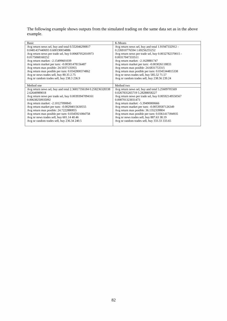
82
The following example shows outputs from the simulated trading on the same data set as in the above
example.
Basic K-Means
Avg return news sel, buy and total 0.552046290817 0.0481437440693 0.600190034886
Avg return news per trade sel, buy 0.00687052010973
0.0175068160252 Avg return market: -2.15499601039
Avg return market per turn: -0.00301478156487
Avg return max posible: 24.5037135955 Avg return max posible per turn: 0.0342800374862
Avg nr news trades sell, buy 80.35 2.75
Avg nr random trades sell, buy 238.3 236.9
Avg return news sel, buy and total 1.91947332912 -0.226910776594 1.69256255252
Avg return news per trade sel, buy 0.0032782370015 -
0.00317047333511 Avg return market: -2.1628881747
Avg return market per turn: -0.003026118833
Avg return max posible: 24.6831753315 Avg return max posible per turn: 0.0345344815338
Avg nr news trades sell, buy 585.52 71.57
Avg nr random trades sell, buy 238.56 239.24
Method one Method two
Avg return news sel, buy and total 2.36817356184 0.258236328338
2.62640989018 Avg return news per trade sel, buy 0.00393947094161
0.00638250935092
Avg return market: -2.10127090845 Avg return market per turn: -0.00294015630555
Avg return max posible: 24.7222880855
Avg return max posible per turn: 0.0345921084758 Avg nr news trades sell, buy 601.14 40.46
Avg nr random trades sell, buy 236.34 240.5
Avg return news sel, buy and total 5.25609705569
0.0267835265719 5.28288058227 Avg return news per trade sel, buy 0.00592149550567
0.000701323031473
Avg return market: -5.39490000666 Avg return market per turn: -0.00539587126349
Avg return max posible: 36.1352339804
Avg return max posible per turn: 0.0361417394935 Avg nr news trades sell, buy 887.63 38.19
Avg nr random trades sell, buy 333.33 333.65