texture analysis for computed tomography...

Texture Analysis for Computed Texture Analysis for Computed Tomography StudiesTomography Studies

Stelu Aioanei, Arati Kurani, Dong-Hui XuCTI Undergraduates

Advisors: Jacob Furst, PhD, Assistant ProfessorDaniela Raicu, PhD, Assistant Professor

CTI, DePaul University

2

Undergraduate ResearchUndergraduate Research

• Research Interests– Data Mining for United States Patent and Trademark Office– Data Mining for Customer Behavior Modeling – Medical Imaging

• Collaborators: Department of Radiology, Northwestern Memorial Hospital, Chicago, IL

• Dr. David Channin, Director of the Department of Radiology• Dr. Alice Averbukh, Research Associate

• Project – Classification of Tissues Using Texture Information in CT

studies

3

• Problem Statement – The classification of human organs using raw data (pixels) from abdominal

and chest CT images– While traditional texture metrics have concentrated on 2D texture, 3D

imaging modalities are becoming more and more prevalent, providing the possibility of examining texture as a volumetric phenomenon

– We expect that texture derived from volumetric data will have better discriminating power than 2D texture derived from slice data, thus increasing the organ classification accuracy

Classification of TissuesClassification of Tissues

heartlabels for the organs

present in the image

backbone

4

SegmentationSegmentation

Organ/Tissue segmentation in

CT images

- Data: 344 DICOM images- Segmented organs: liver, kidneys, spleen, backbone, & heart- Segmentation algorithm: Active Contour Mappings (Snakes)

-A boundary-based segmentation algorithm-Input for the algorithm: a number of initial points & five mainparameters that influence the way the boundary is formed

-The values of the five parameters simulate the action of two forces:-Internal: designed to keep the snake smooth during the deformation-External: designed to move the snake towards the boundary

5

SegmentationSegmentation

6

Texture ModelsTexture Models

• What is texture?– Texture is a measure of the variation of the intensity of a

surface, quantifying properties such as smoothness, coarseness, and regularity

– Texture is a connected set of pixels satisfying a given gray level property which occurs repeatedly in an image region constitutes a textured region

• Texture Models:– Co-occurrence Matrices– Run-Length Matrices

7

CoCo--occurrence Matricesoccurrence Matrices


CT images

Calculate 2DCo-occurrence

Matrices

8

CoCo--occurrence Matricesoccurrence Matrices

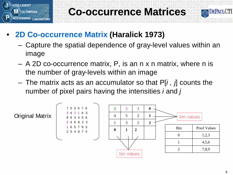
• 2D Co-occurrence Matrix (Haralick 1973)– Capture the spatial dependence of gray-level values within an

image – A 2D co-occurrence matrix, P, is an n x n matrix, where n is

the number of gray-levels within an image – The matrix acts as an accumulator so that P[i , j] counts the

number of pixel pairs having the intensities i and j

210

2231

1254

0152

bin values

bin values

7 5 3 5 7 9 3 4 2 1 6 38 6 3 4 5 6 2 4 6 8 2 3

1 6 5 7 9 3 2 5 4 8 7 4

Original Matrix

7,8,92

4,5,61

1,2,30

Pixel ValuesBin

9

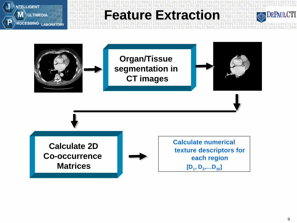
Feature ExtractionFeature Extraction


CT images

Calculate 2DCo-occurrence

Matrices

Calculate numerical texture descriptors for

each region[D1, D2,…D10]

10


• 2D Co-occurrence Matrix (cont.)• In order to quantify this spatial dependence of gray-level values, we

calculate various textural features proposed by Haralick:

– Entropy– Energy (Angular

Second Moment)– Contrast – Homogeneity – SumMean (Mean)

– Variance – Correlation – Maximum Probability– Inverse Difference

Moment– Cluster Tendency

11

2D Results2D Results

• For each slice per organ we average the feature values derived from the 20 matrices, leaving us with a single value per feature per slice:

26.471211.44697.112929.1109217.30890911.662886.63457452.764427.0346923.892828

ClusterTendency

InverseDifferenceMoment

MaximumProbability

CorrelationVarianceSumMeanHomogeneityContrastEnergyEntropy

12



CT images

Calculate numerical texture descriptors for

each organ[D1, D2,…D10]

Calculate Co-occurrence

Matrices forVolumetric Data

13

Volumetric ResultsVolumetric Results

2D dependence matrices that are able to capture the spatial dependence of gray-level values in a set of three-dimensional data (i.e. a set of CT scans for a given patient = single 3D input)

Slice 3

Slice 2

Slice 1

Slice 3

Slice 2

Slice 1

11.0085880.40212950.0960270.09868713.9855911.075230.540800794.933750.037093.80848

ClusterTendency

InverseDifferenceMoment

MaximumProbability

CorrelationVarianceSumMeanHomogeneityContrastEnergyEntropy

14

3D Results 3D Results -- BackboneBackbone

• For each organ, we took the corresponding average feature value and plotted it on the 2D graph (does it fall within min and max?):

• Using the five number summary for 2D data, we defined another range (does the volumetric value fall within Q1 and Q3?):

0.0537575.00000

0.0422650.00000

0.0321125.00000Percentiles

0.07021Maximum

0.01230Minimum

Energy (Mean)

0.01000000000.0200000000

0.03000000000.0400000000

0.05000000000.0600000000

0.07000000000.0800000000

Energy (Mean)

0

2

4

6

8

10

12

14

Fre

qu

ency

Mean = 0.042983678161Std. Dev. = 0.01458000127N = 40

Energy (Mean)

Patient 2 - 0.03746

Patient 1 - 0.03295

Volumetric Data

15

2D and 3D Results2D and 3D Results

432550TOTAL

555Cluster Tendency

315Inverse Difference Moment

525Maximum Probability

425Correlation

555Variance

545SumMean

315Homogeneity

315Contrast

525Energy

525Entropy

Min - MaxQ1 – Q3# of Organs

The distribution of the volumetric co-occurrence descriptors with respect to the 2D data

16

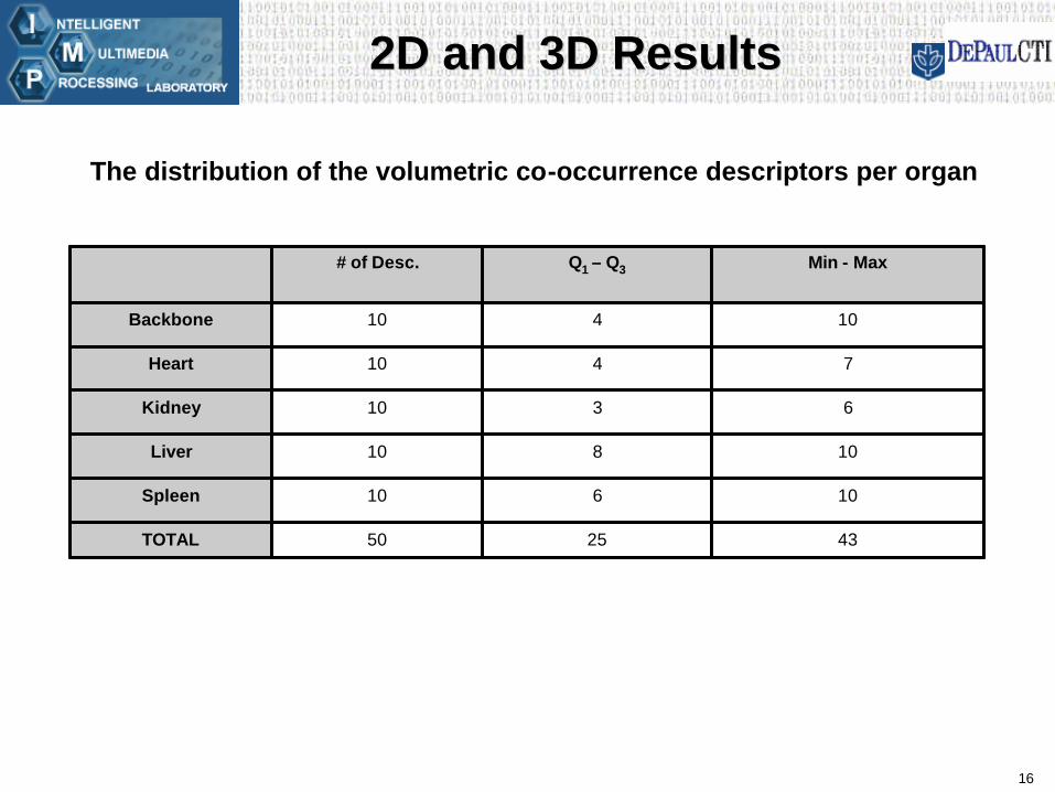
2D and 3D Results2D and 3D Results

432550TOTAL

10610Spleen

10810Liver

6310Kidney

7410Heart

10410Backbone

Min - MaxQ1 – Q3# of Desc.

The distribution of the volumetric co-occurrence descriptors per organ

17

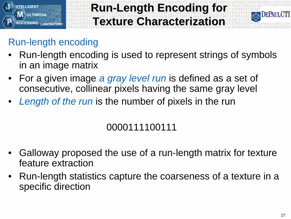
RunRun--Length Encoding for Length Encoding for Texture CharacterizationTexture Characterization

Run-length encoding• Run-length encoding is used to represent strings of symbols

in an image matrix • For a given image a gray level run is defined as a set of

consecutive, collinear pixels having the same gray level• Length of the run is the number of pixels in the run

0000111100111

• Galloway proposed the use of a run-length matrix for texture feature extraction

• Run-length statistics capture the coarseness of a texture in a specific direction

18

Definition of RunDefinition of Run--Length MatricesLength Matrices

1 1 2 2 1 13 3 1 1 2 21 1 2 3 1 13 1 2 2 1 11 1 3 2 2 22 3 1 1 2 2

The run-length matrix p (i, j) is defined by specifying direction and then count the occurrence of runs for each gray levels and length in this direction

(i) Dimension corresponds to the gray level (bin values) and has a length equal to the maximum gray level (bin values) n

(j) dimension corresponds to the run length and has length equal to the maximum run length (bin values)

0000143

0001422

0000811

654321j i0 °

19


• Run-length matrix (cont.)• Eleven texture descriptors are calculated to capture the texture

properties and differentiate among different textures

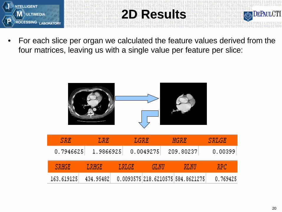
- short run emphasis (SRE)- long run emphasis (LRE)- high gray-level run emphasis (HGRE)- low gray-level run emphasis (LGRE) - Short Run Low Gray-Level Emphasis (SRLGE)- Short Run High Gray-Level Emphasis (SRHGE)- Long Run Low Gray-Level Emphasis (LRLGE)- Long Run High Gray-Level Emphasis (HRHGE)- Gray-Level Non-uniformity (GLNU)- Run Length Non-uniformity (RLNU)- Run Percentage (RPC)

20

2D Results2D Results

• For each slice per organ we calculated the feature values derived from the four matrices, leaving us with a single value per feature per slice:

21

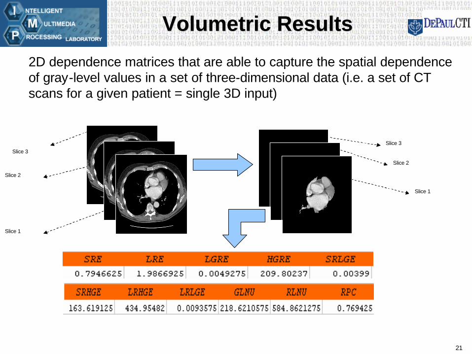
Volumetric ResultsVolumetric Results

Slice 3

Slice 2

Slice 1

Slice 3

Slice 2

Slice 1

2D dependence matrices that are able to capture the spatial dependence of gray-level values in a set of three-dimensional data (i.e. a set of CT scans for a given patient = single 3D input)

22

ResultsResults

• For each organ, we took the corresponding average feature value and plotted it on the 2D graph

• Using the five number summary for 2D data, we defined another range

0.50000 0.55000 0.60000 0.65000 0.70000 0.75000

SRE

0

5

10

15

20

Freq

uenc

y

Mean = 0.5993721Std. Dev. = 0.03982571N = 140

Histogram

0.6291975

0.6001350

0.5706525

0.71057Maximum

0.50515Minimum

perc

entil

eBackbone SRE

23

ResultsResults

• The distribution of the volumetric run-length descriptors with respect to the 2D data

261545total

205rpc

215lrlge

215lrhge

325srhge

405srlge

555hgre

555lgre

315lre

005sre

Min-MaxQ1-Q3# of Organs

24

Results Results

• The distribution of the volumetric run-length descriptors per organ

261545total

529spleen

869liver

229kidney

629heart

539backbone

Min-MaxQ1-Q3# of Desc.

25

ClassificationClassification

Calculate numerical texture descriptors

for each region[D1, D2,…D21

]


CT images

• Motivation:Investigate the feasibility of automated classification of human organ tissues in a chest and abdominal CT image

• Stage 1: Texture feature extraction

Data: 340*4 = 1360 regions of interests Segmented organs: liver, kidneys, spleen,

backbone, & heart

26

ClassificationClassification

IF HGRE <= 0.38 AND ENTROPY > 0.43

AND SRHGE <= 0.20 AND CONTRAST > 0.029

THEN Prediction = HeartProbability = 0.99

Classification rules for tissue/organs

in CT images

Calculate numerical texture descriptors

for each region[D1, D2,…D21

]


CT images

Stage 2: Classifier creationData: 911 training set (66.6%), 449 testing set (33.3%)

27

Classifier CreationClassifier Creation

Decision Tree: A decision tree is a flow-chat-like structure that resembles a tree

28

Classifier CreationClassifier Creation

• Decision rules highlight the most relevant descriptors for the classification of chest and abdominal image

• Classification accuracy parameters- sensitivity- specificity - precision - accuracy

IF ((HGRE <= 0.3788) AND(CLUSTER > 0.0383095 ) AND(GLNU <= 0.03184) AND(LRE <= 0.123405))

THENNode = 17Prediction = BackboneProbability = 1.000000

29

ResultsResults

30

Conclusion and Future WorkConclusion and Future Work

• Conclusion– Using only 21 descriptors it is possible to classify different organ

tissues in the CT images– Combining some other texture models will increase the performance

of the classifier

• Future Work– Improve snake segmentation– Compare the classification result with result obtained using neural

network technique– Use texture descriptors derived from volumetric data to aid the

classification in CT image

texture analysis for computed tomography...

Documents