tfy4235/fys8904 : computational...
TRANSCRIPT

TFY4235/FYS8904 : Computational Physics1
Ingve Simonsen
Department of PhysicsNorwegian University of Science and Technology
Trondheim, Norway
Lecture series, Spring 2018
1Special thanks Profs. Alex Hansen and Morten Hjorth-Jensen for invaluable contributionsTFY4235/FYS8904 Computational Physics – ver2018 1 / 515

General information
LecturesMon. 12:15–14:00 (EL6)Fri. 08:15–09:00 (R8)
ExercisesFri. 09:15–10:00 (R8)
Evaluation and grading
Multi-day take home exam (counts 100% of final grade)Exam date to be decideda
Exercises are not compulsory, but strongly recommended...Three assignments will be given during the semester
Solutions to one of the three will be randomly picked and part of the take-homeexam
aProbably to take place just before the ordinary exam period
Homepagehttp://web.phys.ntnu.no/˜ingves/Teaching/TFY4235/
All relevant information will be posted here!
TFY4235/FYS8904 Computational Physics – ver2018 2 / 515
The aims of the course
Main aim of the classProvide you with a TOOLBOX for solving physical problems on the computer!
For a given problem, you should after completing this class, be able toidentify suitable and efficient methods for solving it numericallywrite programs that use these algorithmsto test you program to make sure it is correctto analyze the resultshave an overview of existing scientific numerical libraries
However, this class will notfocus on the details of the various algorithmsteach you how to program by following the lectures
TFY4235/FYS8904 Computational Physics – ver2018 3 / 515

The aims of the course
In more detail:Develop a critical approach to all steps of a project
which natural laws and physical processes are importantsort out initial conditions and boundary conditions etc.which methods are most relevant
This means to teach you structured scientific computing, learn tostructure a project.A critical understanding of central mathematical algorithms and methodsfrom numerical analysis. Know their limits and stability criteria.Always try to find good checks of your codes (like closed-from solutions)To enable you to develop a critical view on the mathematical model andthe physics.
TFY4235/FYS8904 Computational Physics – ver2018 4 / 515

Programming languages
TFY4235/FYS8904 Computational Physics – ver2018 5 / 515

Which programming language to use?
In principle, you may use any programming language you wish for this class!
Recommended (by me)CC++Fortran 90/2003/2008pythonjulia
Not RecommendedMatlabJavaFortran 77
CommentsPython is the definitely slowest of the recommended languages!Fortran 77 and C are regarded as slightly faster than C++ or Fortran2 .
2For this class, Fortran means Fortran 95/2003/2008 (modern Fortran)TFY4235/FYS8904 Computational Physics – ver2018 6 / 515

“The two-language problem”
“The two-language problem” is also known as Outerhout’s dichotomy (aftercomputer scientist John Ousterhout’s categorization scheme)
High-level programming languages tend to fall into two groupssystem programming languages
hard to use, fast
scripting languageseasy to use, slow
Attempts to get the best of both worlds have tended to result in a bit of a mess.The best option today is Julia in my opinion!
TFY4235/FYS8904 Computational Physics – ver2018 7 / 515

C++ and C
Strong featuresare widely availableportablefast (C++ is slower than C)complex variables can also bedefined in the new ANSI C++/Cstandardsmore and more numericallibraries exist (but still not asmany as for Fortran 77)the efficiency of C++ can beclose to that provided by FortranC++ is rich (about 60 keywords)C++/C is used also outside thescientific/technical communityC++ is an object-orientedlanguage (C is not...)
Weak featuresC++ is a complex language(takes time and experience tomaster)some parts of the languageshould NOT be used fornumerical calculations sincethey are slowerror prone dynamic memorymanagementit is easy in C++ to writeinefficient code (slow)
TFY4235/FYS8904 Computational Physics – ver2018 8 / 515
Fortran
For this class, Fortran means Fortran 95/2003/2008 (modern Fortran)
Strong featureslanguage made for numericalcalculationslarge body of libraries fornumerical calculationsfairly easy to learnportablefastcomplex variables are native tothe languagearray syntax ala Matlabe.g. A(3:5), size(A), min(A)newest versions of Fortran isobject-oriented
Weak featuresFortran is only used in thescientific/technical communityFortran is less rich then C++
TFY4235/FYS8904 Computational Physics – ver2018 9 / 515

python
Strong features
a rich scripting languagefully object-orientedclean syntax gives fast codedevelopmentfree (non-commercial)bindings to many libraries existnumpy and scipy (use them!)easy integration of fast compiledC/C++/Fortran routines
Weak featurescan be slowa scripting language
TFY4235/FYS8904 Computational Physics – ver2018 10 / 515

julia
Strong features
fast : “Just in Time” compilationa rich scripting languagefully object-orientedclean syntax gives fast codedevelopmentfree (non-commercial)bindings to many libraries existinterface an increasing numberof libraries
Weak featuresunder developmentnot so widespread
TFY4235/FYS8904 Computational Physics – ver2018 11 / 515

Choose the “right” language for the job
During the 2014 exam a student found a speedup of a factor 350 whenmoving his code from Matlab to C++!
E.g. if the C-job took 15 min., Matlab will require 5250 h (about 4 days)!
The student said
It was painful to write out the program all over again at first, but after a while I got used to thesyntax and came to understand exactly how much computing power can be saved. A relativelysmall simulation (1000 sweeps on a lattice with L = 100) ran 343 times faster after re-writingthe program in C++!
The biggest lesson for me in this exam has definitely been the value ofprogramming in an efficient language, and I only wish I had more time to makethe C++ program even more efficient.
TFY4235/FYS8904 Computational Physics – ver2018 12 / 515
Literature
The following material represents good reading material for this class:
Press, Flanery, Teukolsky and Vetterling, Numerical Recipes: The Art ofScientific Computing, 3rd ed., Cambridge University Press, 2007.
Morten Hjorth-Jensen, Computational Physics, unpublished, 2013Available from http://web.phys.ntnu.no/˜ingves/Teaching/TFY4235/Download/lectures2013.pdf
For C++ programmers
J. J. Barton and L. R. Nackman,Scientific and Engineering C++, AddisonWesley, 3rd edition 2000.
B. Stoustrup, The C++ programming language, Pearson, 1997.
TFY4235/FYS8904 Computational Physics – ver2018 13 / 515
Numerical libraries
Strong recommendation
Use existing libraries whenever possibleThey are typically more efficient than what you can write yourself
Some important numerical libraries (to be mentioned and discussed later)LAPACK (Fortran 90) [wrapper LAPACK95]BLAS (Fortran 77)GNU Scientific Library (C)Slatec (Fortran 77)
Check out the list of numerical libraries at:http://en.wikipedia.org/wiki/List_of_numerical_libraries
TFY4235/FYS8904 Computational Physics – ver2018 14 / 515
A structured programming approach
Before writing a single line of code, have the algorithm clarified andunderstood. It is crucial to have a logical structure of e.g., the flow andorganization of data before one starts writing.Always try to choose the simplest algorithm. Computational speed can beimproved upon later.Try to write an as clear program as possible. Such programs are easier todebug, and although it may take more time, in the long run it may saveyou time. If you collaborate with other people, it reduces spending timeon debugging and trying to understand what the codes do.
A clear program will also allow you to remember better what the programreally does!
TFY4235/FYS8904 Computational Physics – ver2018 15 / 515
A structured programming approach
The planning of the program should be from top down to bottom, trying tokeep the flow as linear as possible. Avoid jumping back and forth in theprogram. First you need to arrange the major tasks to be achieved. Thentry to break the major tasks into subtasks. These can be represented byfunctions or subprograms. They should accomplish limited tasks and asfar as possible be independent of each other. That will allow you to usethem in other programs as well.
Try always to find some cases where an analytic solution exists or wheresimple test cases can be applied. If possible, devise different algorithmsfor solving the same problem. If you get the same answers, you may havecoded things correctly or made the same error twice or more.
Warning
Remember, a compiling code does not necessarily mean a correct program!
TFY4235/FYS8904 Computational Physics – ver2018 16 / 515

Section 1
Introduction
TFY4235/FYS8904 Computational Physics – ver2018 17 / 515

Outline I
1 Introduction
2 Number representation and numerical precision
3 Finite differences and interpolation
4 Linear algebra
5 How to install libraries on a Linux system
6 Eigenvalue problems
7 Spectral methods
8 Numerical integration
TFY4235/FYS8904 Computational Physics – ver2018 18 / 515

Outline II9 Random numbers
10 Ordinary differential equations
11 Partial differential equations
12 Optimization
TFY4235/FYS8904 Computational Physics – ver2018 19 / 515

What is Computational Physics (CP)?
University of California at San Diego (UCSD)3
“Computational physics is a rapidly emerging new field covering a wide range ofdisciplines based on collaborative efforts of mathematicians, computer scientists,and researchers from many areas of pure and applied physics. This newapproach has had a decisive influence on fields that traditionally have beencomputationally intensive, and is expected to change the face of disciplines thathave not commonly been associated with high performance computation.
By its very nature, computational physics is strongly interdisciplinary, withmethodologies that span the traditional boundaries between fields, allowingexperts in this area a more flexible position in today’s competitive employmentarena.”
Wikipedia tries the following definition:“Computational physics is the study and implementation of numericalalgorithms to solve problems in physics for which a quantitative theoryalready exists” (not a good definition in my opinion)
3http://www-physics.ucsd.edu/students/courses/winter2010/physics141/
TFY4235/FYS8904 Computational Physics – ver2018 20 / 515
What is Computational Physics (CP)?
DefinitionComputational physics is the science of using computers to assist in thesolution of physical problems, and to conduct further physics research
1 Discretized analytic calculations2 Algorithmic modelling3 Data treatment (e.g. CERN)
Computational physics is the “third way” of physics alongsideexperimental and theoretical physicsCP is a separate and independent branch of physicsSystems are studied by “numerical experiments”Computational physics is interdisciplinary
TFY4235/FYS8904 Computational Physics – ver2018 21 / 515

What is Computational Physics?
Some examples of areas that lie within the scope of computational physics
Large scale quantum mechanical calculations in nuclear, atomic,molecular and condensed matter physicsLarge scale calculations in such fields as hydrodynamics, astrophysics,plasma physics, meteorology and geophysicsSimulation and modelling of complex physical systems such as those thatoccur in condensed matter physics, medical physics and industrialapplicationsExperimental data processing and image processingComputer algebra; development and applicationsThe online interactions between physicist and the computer systemEncouragement of professional expertise in computational physics inschools and universities
Source : Institute of Physics
TFY4235/FYS8904 Computational Physics – ver2018 22 / 515

Why Computational Physics?
Physics problems are in general very difficult to solve exactlyanalytically solutions are the exceptions. . . not the rule
Real-life problems often cannot be solved in closed form, due tolack of algebraic and/or analytic solubilitycomplex and/or chaotic behaviortoo many equations to render an analytic solution practical
Some examples :a bouncing ballthe physical pendulum satisfying the differential equation
d2θ(t)dt2 +
g`
sin θ(t) = 0
system of interacting spheres (studies by e.g. molecular dynamics)the Navier-Stokes equations (non-linear equations)quantum mechanics of moleculesetc. etc
On the computer, one can study many complex real-life problems!
TFY4235/FYS8904 Computational Physics – ver2018 23 / 515
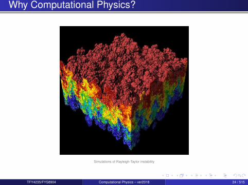
Why Computational Physics?
Simulations of Rayleigh-Taylor instability
TFY4235/FYS8904 Computational Physics – ver2018 24 / 515
Detailed simple examples of the use of CP
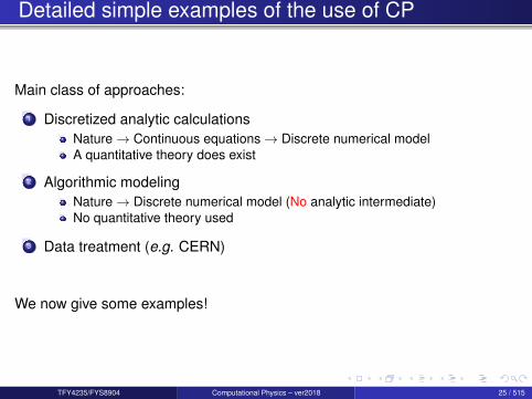
Main class of approaches:
1 Discretized analytic calculationsNature→ Continuous equations→ Discrete numerical modelA quantitative theory does exist
2 Algorithmic modelingNature→ Discrete numerical model (No analytic intermediate)No quantitative theory used
3 Data treatment (e.g. CERN)
We now give some examples!
TFY4235/FYS8904 Computational Physics – ver2018 25 / 515
Example 1: Laplace equation
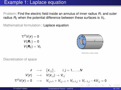
Problem: Find the electric field inside an annulus of inner radius R1 and outerradius R2 when the potential difference between these surfaces is V0.
Mathematical formulation : Laplace equation
∇2V (r) = 0V (R1) = 0V (R2) = V0
Geometry under study
Discretization of space
r −→
r i,j, i , j = 1, . . . ,N
V (r) −→ V (r i,j )→ Vi,j
∇2V (r) = 0 −→ Vi,j+1 + Vi,j−1 + Vi+1,j + Vi−1,j − 4Vi,j = 0
TFY4235/FYS8904 Computational Physics – ver2018 26 / 515

Example 1: Laplace equation
values of the potential on the boundary are known|r i,j | ≈ R1 : Vi,j = 0|r i,j | ≈ R2 : Vi,j = V0
this modifies the equations for points close to the surface
Vi,j+1 + Vi,j−1 + Vi+1,j + Vi−1,j − 4Vi,j = 0
so that known values gives raise to a right-hand-sidea linear system (in
Vi,j
) is formed
Linear system
Discretization of Laplace equation results in a linear system
Solving a linear system, solves the original continuous problem
Av = b where v =[V11 V21 . . . VNN
]TTFY4235/FYS8904 Computational Physics – ver2018 27 / 515

Example 2: Diffusion-Limited Aggregation (DLA)
Consider the following systemsmall (colloidal) particles diffuse in a liquidplace a sticky ball in the liquidwhen a particle hits the surface of the ball it sticks
Question : What does the structure formed by this process look like?
Challenge
How can one address this question?
TFY4235/FYS8904 Computational Physics – ver2018 28 / 515
Example 2: Diffusion-Limited Aggregation (DLA)
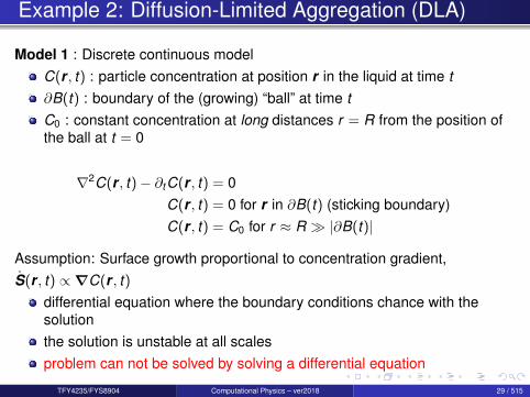
Model 1 : Discrete continuous modelC(r , t) : particle concentration at position r in the liquid at time t∂B(t) : boundary of the (growing) “ball” at time tC0 : constant concentration at long distances r = R from the position ofthe ball at t = 0
∇2C(r , t)− ∂tC(r , t) = 0C(r , t) = 0 for r in ∂B(t) (sticking boundary)C(r , t) = C0 for r ≈ R |∂B(t)|
Assumption: Surface growth proportional to concentration gradient,S(r , t) ∝∇C(r , t)
differential equation where the boundary conditions chance with thesolutionthe solution is unstable at all scalesproblem can not be solved by solving a differential equation
TFY4235/FYS8904 Computational Physics – ver2018 29 / 515

Example 2: Diffusion-Limited Aggregation (DLA)
Model 2 : Algorithmic modeling
consider a large number of particlesindividual particles do random walksthey stick to the boundary the first time they hit it
This model renders a description that fits quantitatively what is seen in nature(examples next slide)
Algorithmic modeling
Nature is modeled directly!
TFY4235/FYS8904 Computational Physics – ver2018 30 / 515

Example 2: Diffusion-Limited Aggregation (DLA)
Experiments
A DLA cluster grown from a copper sulfate solution in an electrodeposition
cell
Simulations
A DLA consisting about 33, 000 particles obtained by allowing random
walkers to adhere to a seed at the center. Different colors indicate different
arrival time of the random walkers.
DLA clusters in 2D have fractal dimension : D ≈ 1.7
TFY4235/FYS8904 Computational Physics – ver2018 31 / 515

Example 3: Bak-Sneppen ModelPhys. Rev. Lett. 71, 4083 (1993)
The model deals with evolutionary biology.
a simple model of co-evolution between interacting speciesdeveloped to show how self-organized criticality may explain key featuresof fossil records
the distribution of sizes of extinction eventsthe phenomenon of punctuated equilibrium
Reference :The “Bak-Sneppen” paper : Phys. Rev. Lett. 71, 4083 (1993)
See also : Phys. Rev. Lett. 76, 348 (1996)
TFY4235/FYS8904 Computational Physics – ver2018 32 / 515

Example 3: Bak-Sneppen ModelPhys. Rev. Lett. 71, 4083 (1993)
Two opposing theory of evolution:phyletic gradualismpunctuated equilibrium (1972)
TFY4235/FYS8904 Computational Physics – ver2018 33 / 515
Example 3: Bak-Sneppen ModelPhys. Rev. Lett. 71, 4083 (1993)
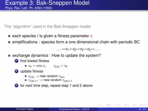
The “algorithm” used in the Bak-Sneppen model
each species i is given a fitness parameter ri
simplifications : species form a one dimensional chain with periodic BC
. . . —r1—r2—r3—r4—. . .
exchange dynamics : How to update the system?1 find lowest fitness
rw = mini ri , ri(w) = rw
2 update fitnessri(w) → new random ri(w)
ri(w)±1 → new random ri(w)±1
3 for next time step, repeat step 1 and 2 above
TFY4235/FYS8904 Computational Physics – ver2018 34 / 515
Summary : Algorithmic modeling
Algorithmic modeling
Nature is modeled directly!
Normally quantitative theories do not exist for such problems
For instance, Diffusion-Limited Aggregation cannot be described by adifferential equation!
TFY4235/FYS8904 Computational Physics – ver2018 35 / 515

Topics
TFY4235/FYS8904 Computational Physics – ver2018 36 / 515

Topics covered by the classTentative list and order
Numerical precisionInterpolation and extrapolationNumerical derivation and integrationRandom numbers and Monte Carlo integrationLinear algebraEigensystemsNon-linear equations and roots of polynomialsFourier and Wavelet transformsOptimization (maximization/minimization)Monte Carlo methods in statistical physicsOrdinary differential equationsPartial differential equationsEigenvalue problemsIntegral equationsParallelization of codes (if time allows)
TFY4235/FYS8904 Computational Physics – ver2018 37 / 515

Section 2
Number representation and numerical precision
TFY4235/FYS8904 Computational Physics – ver2018 38 / 515

Outline I
1 Introduction
2 Number representation and numerical precision
3 Finite differences and interpolation
4 Linear algebra
5 How to install libraries on a Linux system
6 Eigenvalue problems
7 Spectral methods
8 Numerical integration
TFY4235/FYS8904 Computational Physics – ver2018 39 / 515

Outline II9 Random numbers
10 Ordinary differential equations
11 Partial differential equations
12 Optimization
TFY4235/FYS8904 Computational Physics – ver2018 40 / 515
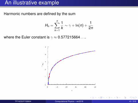
An illustrative example
Harmonic numbers are defined by the sum
Hn =n∑
k=1
1k∼ γ + ln(n) +
12n
where the Euler constant is γ ≈ 0.577215664 . . ..
TFY4235/FYS8904 Computational Physics – ver2018 41 / 515

An illustrative example
Results for Hn (in single precision) for different values of n:
n = 10Asymptotic = 2.92980075Forward sum = 2.92896843 -8.32319260E-04Backward sum = 2.92896843 -8.32319260E-04
n = 100 000Asymptotic = 12.0901461Forward sum = 12.0908508 7.04765320E-04Backward sum = 12.0901527 6.67572021E-06
Question : Why is the backward sum more accurate?
TFY4235/FYS8904 Computational Physics – ver2018 42 / 515

How numbers are represented
Numbers→ words (i.e. strings of bits)May have length 32 or 64 or ...
Consequence
Only a limited range of numbers may be represented with infinite precision.Otherwise, always an approximation.
TFY4235/FYS8904 Computational Physics – ver2018 43 / 515

Finite numerical precision
Serious problem with the representation of numbers
A computer has finite numerical precision!
Potential problems in representing integer, real, and complex numbersOverflowUnderflowRoundoff errorsLoss of precision
TFY4235/FYS8904 Computational Physics – ver2018 44 / 515
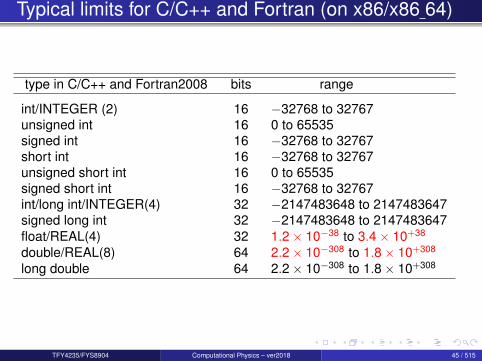
Typical limits for C/C++ and Fortran (on x86/x86 64)
type in C/C++ and Fortran2008 bits range
int/INTEGER (2) 16 −32768 to 32767unsigned int 16 0 to 65535signed int 16 −32768 to 32767short int 16 −32768 to 32767unsigned short int 16 0 to 65535signed short int 16 −32768 to 32767int/long int/INTEGER(4) 32 −2147483648 to 2147483647signed long int 32 −2147483648 to 2147483647float/REAL(4) 32 1.2× 10−38 to 3.4× 10+38
double/REAL(8) 64 2.2× 10−308 to 1.8× 10+308
long double 64 2.2× 10−308 to 1.8× 10+308
TFY4235/FYS8904 Computational Physics – ver2018 45 / 515

Typical limits for C/C++ and Fortran (on x86/x86 64)
How do we find these constants?
Fortran90 program:
program test_huge_tiny_epsilonimplicit nonewrite(*,*) huge(0), huge(0.0), huge(0.0d0)write(*,*) tiny(0.0), tiny(0.0d0)write(*,*) epsilon(0.0), epsilon(0.0d0)
end program test_huge_tiny_epsilon
Output:
˜/Tmp tux => gfortran huge_tiny.f90 -o test_tiny_huge_epsilon˜/Tmp tux => test_tiny_huge_epsilon2147483647 3.40282347E+38 1.7976931348623157E+308
1.17549435E-38 2.2250738585072014E-3081.19209290E-07 2.2204460492503131E-016
TFY4235/FYS8904 Computational Physics – ver2018 46 / 515
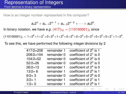
Representation of IntegersFrom decimal to binary representation
How is an integer number represented in the computer?
an2n + an−12n−1 + an−22n−2 + · · ·+ a020.
In binary notation, we have e.g. (417)10 = (110100001)2 since
(110100001)2 = 1×28+1×27+0×26+1×25+0×24+0×23+0×22+0×22+0×21+1×20.
To see this, we have performed the following integer divisions by 2
417/2=208 remainder 1 coefficient of 20 is 1208/2=104 remainder 0 coefficient of 21 is 0104/2=52 remainder 0 coefficient of 22 is 052/2=26 remainder 0 coefficient of 23 is 026/2=13 remainder 1 coefficient of 24 is 013/2= 6 remainder 1 coefficient of 25 is 16/2= 3 remainder 0 coefficient of 26 is 03/2= 1 remainder 1 coefficient of 27 is 11/2= 0 remainder 1 coefficient of 28 is 1
TFY4235/FYS8904 Computational Physics – ver2018 47 / 515

Representation of floating-point numbers
A floating-point number, x , can be represented by:
x = (s,m,e)b = (−1)s ×m × be
s the sign: positive (s = 0) or negative (s = 1)m the mantissa (significand or coefficient)e the exponentb the base: b = 2 (binary) or b = 10 (decimal)
Example : (1,12345,−3)10 = (−1)1 × 12345× 10−3 = −12.345
Warning
Floating point representations vary from machine to machine!However, the IEEE 754 standard is quite common
TFY4235/FYS8904 Computational Physics – ver2018 48 / 515
Representation of floating-point numbers
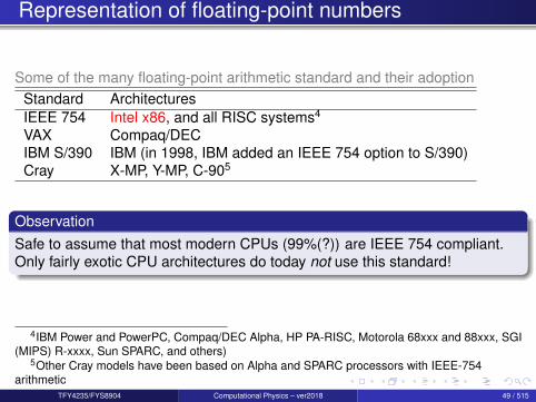
Some of the many floating-point arithmetic standard and their adoptionStandard ArchitecturesIEEE 754 Intel x86, and all RISC systems4
VAX Compaq/DECIBM S/390 IBM (in 1998, IBM added an IEEE 754 option to S/390)Cray X-MP, Y-MP, C-905
ObservationSafe to assume that most modern CPUs (99%(?)) are IEEE 754 compliant.Only fairly exotic CPU architectures do today not use this standard!
4IBM Power and PowerPC, Compaq/DEC Alpha, HP PA-RISC, Motorola 68xxx and 88xxx, SGI(MIPS) R-xxxx, Sun SPARC, and others)
5Other Cray models have been based on Alpha and SPARC processors with IEEE-754arithmetic
TFY4235/FYS8904 Computational Physics – ver2018 49 / 515

Representation of floating-point numbers
In a typical computer base b = 2 (binary representation) is used and one putsrestrictions on m and e (imposed by the available word length).
The mantissathe leftmost binary digit of m is 1this means, m is normalized; moved to the left as far as possibleleading bit of m (always 1) is not stored(24 bits information storeable in 23 bits)
The exponente is given uniquely from the requirements on madd to e a machine dependent exponential bias e0 so that e + e0 > 0one store e + e0 > 0 in the floating-point representation
TFY4235/FYS8904 Computational Physics – ver2018 50 / 515

Representation of floating-point numbers
Storage convention (for IEEE 754 floating-numbers)
x −→ | s︸︷︷︸sign
| e + e0︸ ︷︷ ︸exponent
| m − 1︸ ︷︷ ︸mantissa
| = s e + e0 m-1
e + e0 is a positive integer
m the mantissam = (1.a−1a−2 . . . a−23)2 = 1× 20 + a−1× 2−1 + +a−2× 2−2 + · · ·+ a−23× 2−23
only the faction m − 1 of the mantissa is stored, i.e. the an ’sthe leading bit of m is not stored)23 bits used to represent 24 bits of information when using single precision
Storage size
Size in bits used in the IEEE 754 standard (most modern computers)Type Sign Exponent Mantissa Total bits Exponent bias Bits precision Decimal digits
Single 1 8 23 32 127 24 ∼7.2Double 1 11 52 64 1024 53 ∼15.9Quadruple 1 15 112 128 16383 113 ∼34.0
For more information see http://en.wikipedia.org/wiki/Floating_pointTFY4235/FYS8904 Computational Physics – ver2018 51 / 515
Representation of floating-point numbersSome examples: IEEE 754 floating-points
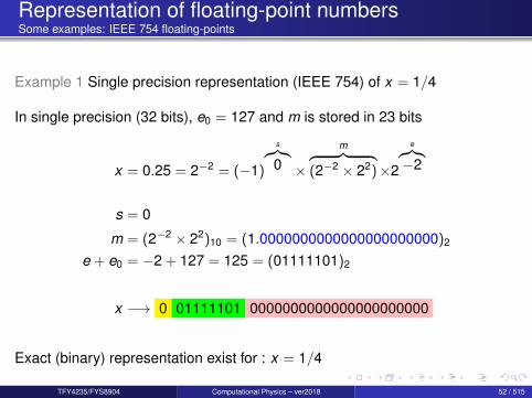
Example 1 Single precision representation (IEEE 754) of x = 1/4
In single precision (32 bits), e0 = 127 and m is stored in 23 bits
x = 0.25 = 2−2 = (−1)
s︷︸︸︷0 ×
m︷ ︸︸ ︷(2−2 × 22)×2
e︷︸︸︷−2
s = 0
m = (2−2 × 22)10 = (1.0000000000000000000000)2
e + e0 = −2 + 127 = 125 = (01111101)2
x −→ 0 01111101 0000000000000000000000
Exact (binary) representation exist for : x = 1/4
TFY4235/FYS8904 Computational Physics – ver2018 52 / 515

Representation of floating-point numbersSome examples: IEEE 754 floating-points
Example 2
Single precision representation (IEEE 754) of x = 2/3
x =23
= (−1)
s︷︸︸︷0 ×
m︷ ︸︸ ︷(2/3× 21)×2
e︷︸︸︷−1
x = (0.10101010 . . .)2 = (1.0101010 . . .)2︸ ︷︷ ︸m
×2−1
s = 0
m = (2/3× 21)10 = (1.01010101010101010 . . .)2
e + e0 = −1 + 127 = 126 = (01111110)2
x −→ 0 01111110 01010101010101010101011
Representation of x = 2/3 is an approximation!TFY4235/FYS8904 Computational Physics – ver2018 53 / 515

Representation of floating-point numbersSome examples: IEEE 754 floating-points
Example 3
Convert the following 32 bits (IEEE 754) binary number to decimal format:
x −→ 1 01111101 11101000000000000000000
This gives
s = 1e + e0 = (01111101)2 = 125 ⇒ e = 125− 127 = −2
m = (1.11101000000000000000000)2
= 20 + 2−1 + 2−2 + 2−3 + 2−5 ≈ (1.906250)10
so that
x = (−1)s ×m × 2e = (−0.4765625 . . .)10
TFY4235/FYS8904 Computational Physics – ver2018 54 / 515

Representation of floating-point numbersExtra material
In the decimal system we would write a number like 9.90625 in what is calledthe normalized scientific notation.
9.90625 = 0.990625× 101,
and a real non-zero number could be generalized as
x = ±r × 10n,
with r a number in the range 1/10 ≤ r < 1. In a similar way we can userepresent a binary number in scientific notation as
x = ±q × 2m,
with q a number in the range 1/2 ≤ q < 1. This means that the mantissa of abinary number would be represented by the general formula
(0.a−1a−2 . . . a−n)2 = a−1 × 2−1 + a−2 × 2−2 + · · ·+ a−n × 2−n.
TFY4235/FYS8904 Computational Physics – ver2018 55 / 515
Representation of floating-point numbersExtra material
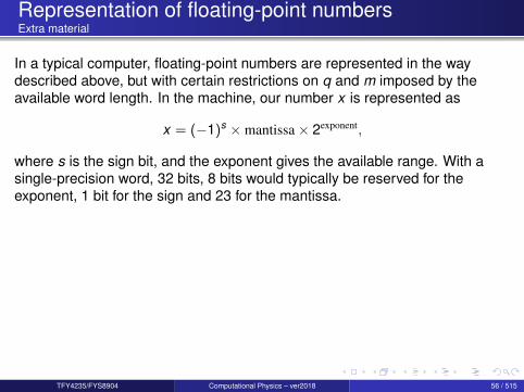
In a typical computer, floating-point numbers are represented in the waydescribed above, but with certain restrictions on q and m imposed by theavailable word length. In the machine, our number x is represented as
x = (−1)s ×mantissa× 2exponent,
where s is the sign bit, and the exponent gives the available range. With asingle-precision word, 32 bits, 8 bits would typically be reserved for theexponent, 1 bit for the sign and 23 for the mantissa.
TFY4235/FYS8904 Computational Physics – ver2018 56 / 515

Representation of floating-point numbersExtra material
A modification of the scientific notation for binary numbers is to require thatthe leading binary digit 1 appears to the left of the binary point. In this casethe representation of the mantissa q would be (1.f )2 and 1 ≤ q < 2. This formis rather useful when storing binary numbers in a computer word, since wecan always assume that the leading bit 1 is there. One bit of space can thenbe saved meaning that a 23 bits mantissa has actually 24 bits. This meansexplicitely that a binary number with 23 bits for the mantissa reads
(1.a−1a−2 . . . a−23)2 = 1× 20 + a−1 × 2−1 + +a−2 × 2−2 + · · ·+ a−23 × 2−23.
As an example, consider the 32 bits binary number
(10111110111101000000000000000000)2,
where the first bit is reserved for the sign, 1 in this case yielding a negativesign. The exponent m is given by the next 8 binary numbers 01111101resulting in 125 in the decimal system.
TFY4235/FYS8904 Computational Physics – ver2018 57 / 515

Representation of floating-point numbersExtra material
However, since the exponent has eight bits, this means it has 28 − 1 = 255possible numbers in the interval −128 ≤ m ≤ 127, our final exponent is125− 127 = −2 resulting in 2−2. Inserting the sign and the mantissa yieldsthe final number in the decimal representation as
−2−2 (1× 20 + 1× 2−1 + 1× 2−2 + 1× 2−3 + 0× 2−4 + 1× 2−5) =
(−0.4765625)10.
In this case we have an exact machine representation with 32 bits (actually,we need less than 23 bits for the mantissa).If our number x can be exactly represented in the machine, we call x amachine number. Unfortunately, most numbers cannot and are thereby onlyapproximated in the machine. When such a number occurs as the result ofreading some input data or of a computation, an inevitable error will arise inrepresenting it as accurately as possible by a machine number.
TFY4235/FYS8904 Computational Physics – ver2018 58 / 515
How the computer performs elementary operationsAddition and subtraction
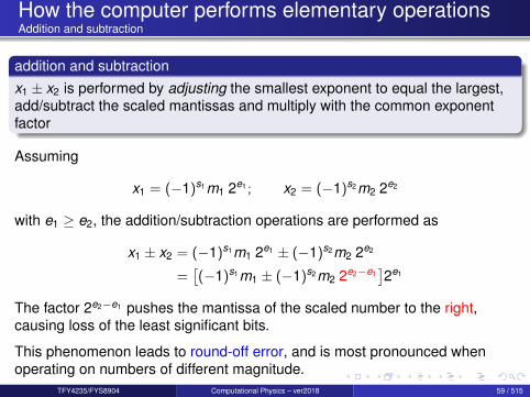
addition and subtractionx1 ± x2 is performed by adjusting the smallest exponent to equal the largest,add/subtract the scaled mantissas and multiply with the common exponentfactor
Assuming
x1 = (−1)s1m1 2e1 ; x2 = (−1)s2m2 2e2
with e1 ≥ e2, the addition/subtraction operations are performed as
x1 ± x2 = (−1)s1m1 2e1 ± (−1)s2m2 2e2
=[(−1)s1m1 ± (−1)s2m2 2e2−e1
]2e1
The factor 2e2−e1 pushes the mantissa of the scaled number to the right,causing loss of the least significant bits.
This phenomenon leads to round-off error, and is most pronounced whenoperating on numbers of different magnitude.
TFY4235/FYS8904 Computational Physics – ver2018 59 / 515

How the computer performs elementary operationsAddition and subtraction
Example (assuming single (32 bits) precision)
y =(0.4765625)10 + (0.0000100)10
=(1.90625 · 2−2)10 + (1.31072 · 2−17)10
= 0 (125)10 (0.90625)10 + 0 (110)10 (0.31072)10
= 0 (125)10 (0.90625 + 1.31072 · 2−15)10
= 0 (125)10 (0.90625 + 0.00004)10
= 0 (125)10 (0.90629)10
TFY4235/FYS8904 Computational Physics – ver2018 60 / 515

How the computer performs elementary operationsAddition and subtraction
Using proper IEEE 754 floating point notation one gets
y =(0.4765625)10 + (0.0000100)10
= 0 01111101 11101000000000000000000 +
0 01101110 01001111100010110101100 (24 − 21 + 20 = 15)
= 0 01111101 11101000000000000000000 +
0 01111101 00000000000000101001111 100010110101100 (lost bits)
≈ 0 01111101 11101000000000101010000 (rounding)
Right shifting
Since the mantissa is 23 bits, and we need to shift to the right GREATERTHAN 23 bits in order to make the exponents equal (don’t forget the hiddenbit)
Converter : http://www.binaryconvert.com/result_float.htmlTFY4235/FYS8904 Computational Physics – ver2018 61 / 515
How the computer performs elementary operationsAddition and subtraction
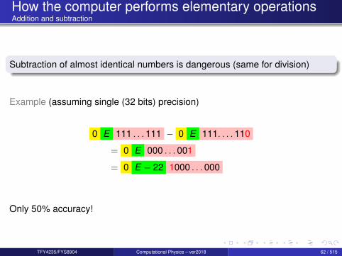
Subtraction of almost identical numbers is dangerous (same for division)
Example (assuming single (32 bits) precision)
0 E 111 . . . 111 − 0 E 111. . . .110
= 0 E 000 . . . 001
= 0 E − 22 1000 . . . 000
Only 50% accuracy!
TFY4235/FYS8904 Computational Physics – ver2018 62 / 515
How the computer performs elementary operationsAddition and subtraction
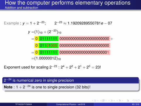
Example : y = 1 + 2−23; 2−23 ≈ 1.19209289550781e − 07
y =(1)10 + (2−23)10
= 0 01111111 00000000000000000000000 +
0 01101000 00000000000000000000000
= 0 01111111 00000000000000000000001=(1.00000012)10
Exponent used for scaling 2−23 : 24 + 22 + 21 + 20 = 23!
2−24 is numerical zero in single precision
Note : 1 + 2−24 is one to single precision (32 bits)!
TFY4235/FYS8904 Computational Physics – ver2018 63 / 515

Machine precision
DefinitionThe smallest number that can be added to 1 giving a result different from 1;i.e. smallest x such that 1 + x > 1
This results in the following machine precision :Single precision (32 bits) : 2−23 ≈ 1.1921 · 10−7 ∼ 10−7
Double precision (64 bits) : 2−52 ≈ 2.2204 · 10−16 ∼ 10−16
Quadruple precision (128 bits) : 2−112 ≈ 1.9259 · 10−34 ∼ 10−34
(non-standard)
Fortran90 has inquiry functions for these numbersSingle prec. : epsilon(1.0)Double prec. : epsilon(1.0D0)!
TFY4235/FYS8904 Computational Physics – ver2018 64 / 515
How the computer performs elementary operationsMultiplication and division
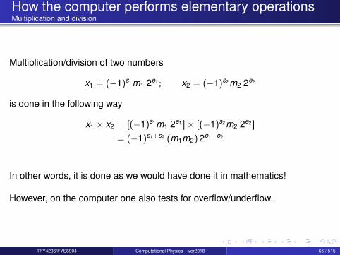
Multiplication/division of two numbers
x1 = (−1)s1m1 2e1 ; x2 = (−1)s2m2 2e2
is done in the following way
x1 × x2 = [(−1)s1m1 2e1 ]× [(−1)s2m2 2e2 ]
= (−1)s1+s2 (m1m2) 2e1+e2
In other words, it is done as we would have done it in mathematics!
However, on the computer one also tests for overflow/underflow.
TFY4235/FYS8904 Computational Physics – ver2018 65 / 515
Loss of precision: Some examples
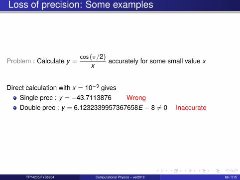
Problem : Calculate y =cos (π/2)
xaccurately for some small value x
Direct calculation with x = 10−9 givesSingle prec : y = −43.7113876 WrongDouble prec : y = 6.1232339957367658E − 8 6= 0 Inaccurate
TFY4235/FYS8904 Computational Physics – ver2018 66 / 515

Loss of precision: Some examples
Problem : For x = 0.0001 calculate
y1(x) =1− cos x
sin x, y2(x) =
sin x1 + cos x
Analytically we have y1(x) = y2(x) which for the given value of xapproximates to ≈ 5.0000000041633333361 . . . × 10−5.
Calculation of y1(x)
Single prec : y1(x) = 0.00000000 WrongDouble prec : y1(x) = 4.9999999779459782E − 005 Inaccurate
Calculation of y2(x)
Single prec : y2(x) = 4.99999987E − 05 AccurateDouble prec : y2(x) = 5.0000000041666671E − 005 Inaccurate
TFY4235/FYS8904 Computational Physics – ver2018 67 / 515
Loss of precision: Some examples
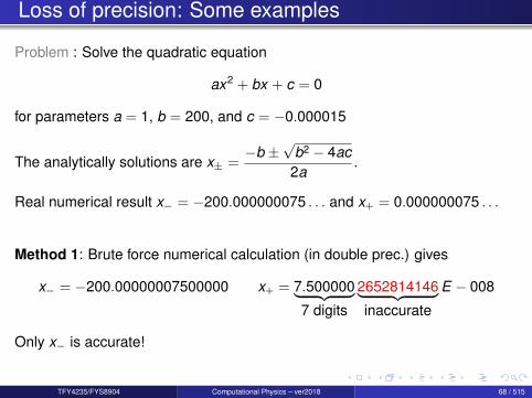
Problem : Solve the quadratic equation
ax2 + bx + c = 0
for parameters a = 1, b = 200, and c = −0.000015
The analytically solutions are x± =−b ±
√b2 − 4ac
2a.
Real numerical result x− = −200.000000075 . . . and x+ = 0.000000075 . . .
Method 1: Brute force numerical calculation (in double prec.) gives
x− = −200.00000007500000 x+ = 7.500000︸ ︷︷ ︸7 digits
2652814146︸ ︷︷ ︸inaccurate
E − 008
Only x− is accurate!
TFY4235/FYS8904 Computational Physics – ver2018 68 / 515

Loss of precision: Some examples
Method 2: Rewrite the solution in the form
x− =−b − sgn(b)
√b2 − 4ac
2a, x+ =
2c−b − sgn(b)
√b2 − 4ac
=c
ax−
x− = −200.00000007500000 x+ = 7.49999999︸ ︷︷ ︸9 digits
71874996E − 008
Now x+ has 2 extra correct digits!
What is the problem?When b2 4ac like here, one has
x− : result OKx+ : catastrophic cancellation
Reference :D. Goldberg, What Every Computer Scientist Should Know About Floating-Point Arithmetic,ACM Computing Surveys 23, 5 (1991).
TFY4235/FYS8904 Computational Physics – ver2018 69 / 515

Computer architectures
The main computer architectures of today are:Distributed memory computersShared memory computers
TFY4235/FYS8904 Computational Physics – ver2018 70 / 515

Section 3
Finite differences and interpolation
TFY4235/FYS8904 Computational Physics – ver2018 71 / 515
Outline I
1 Introduction
2 Number representation and numerical precision
3 Finite differences and interpolationFinite difference approximationsInterpolation schemesDifferentiation schemes
4 Linear algebra
5 How to install libraries on a Linux system
6 Eigenvalue problems
7 Spectral methods
TFY4235/FYS8904 Computational Physics – ver2018 72 / 515

Outline II8 Numerical integration
9 Random numbers
10 Ordinary differential equations
11 Partial differential equations
12 Optimization
TFY4235/FYS8904 Computational Physics – ver2018 73 / 515
How to approximate derivatives
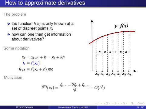
The problem
the function f (x) is only known at aset of discreet points xk
how can one then get informationabout derivatives?
Some notation
xk = xk−1 + h = x0 + khfk ≡ f (xk )
fk+1 ≡ f (xk + h) etc
Motivation
f (2)(xk ) =fk+1 − 2fk + fk−1
h2 +O(h2)
TFY4235/FYS8904 Computational Physics – ver2018 74 / 515
How to approximate derivatives
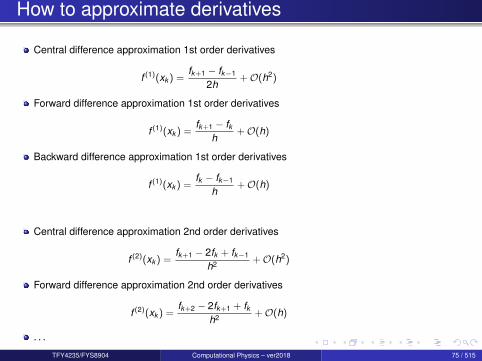
Central difference approximation 1st order derivatives
f (1)(xk ) =fk+1 − fk−1
2h+O(h2)
Forward difference approximation 1st order derivatives
f (1)(xk ) =fk+1 − fk
h+O(h)
Backward difference approximation 1st order derivatives
f (1)(xk ) =fk − fk−1
h+O(h)
Central difference approximation 2nd order derivatives
f (2)(xk ) =fk+1 − 2fk + fk−1
h2 +O(h2)
Forward difference approximation 2nd order derivatives
f (2)(xk ) =fk+2 − 2fk+1 + fk
h2 +O(h)
. . .
TFY4235/FYS8904 Computational Physics – ver2018 75 / 515

How to approximate derivatives
Some higher order finite central difference approximations:
1st order derivatives
f (1)(xk ) =−fk+2 + 8fk+1 − 8fk−1 + fk−2
12h+O(h4)
2nd order derivatives
f (2)(xk ) =−fk+2 + 16fk+1 − 30fk + 16fk−1 − fk−2
12h2 +O(h4)
Question: How to obtain such approximations?
TFY4235/FYS8904 Computational Physics – ver2018 76 / 515

How to approximate derivatives
Say that we wanted a finite difference approximation to f (2)(xi ) but now usingthe three points xk , xk+1 and xk+2. How can this be done?Write
f (2)(xk ) = c0fk + c1fk+1 + c2fk+2 + ε(h)︸︷︷︸error
To determine the c′k ’s, Taylor expand fk+n = f (xk+n) around xk to give thesystem 1 1 1
0 h 2h0 h2
2!(2h)2
2!
c0c1c2
=
001
=⇒
c0c1c2
=1h2
1−21
or
f (2)(xk ) =fk − 2fk+1 + fk+2
h2 +O(h)
3-point forward differences
TFY4235/FYS8904 Computational Physics – ver2018 77 / 515

Finite Difference Operators
Define the following finite difference operators
Forward differences
∆hfk = fk+1 − fk = ∆h[f ](xk )
and higher-order differences obtained by induction [∆2hfk = ∆h(∆hfk ) ]
∆nhfk =
n∑i=0
(−1)i(
ni
)fk+n−i = ∆n
h[f ](xk )
Backward differences
∇hfk = fk − fk−1 = ∇h[f ](xk )
iterations gives
∇nhfk =
n∑i=0
(−1)i(
ni
)fk−n+i = ∇n
h[f ](xk )
TFY4235/FYS8904 Computational Physics – ver2018 78 / 515
Finite Difference Operators
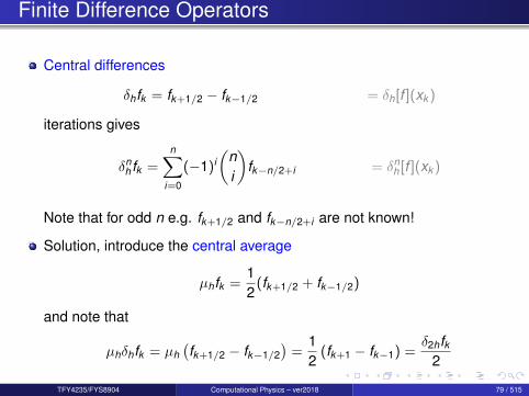
Central differences
δhfk = fk+1/2 − fk−1/2 = δh[f ](xk )
iterations gives
δnh fk =
n∑i=0
(−1)i(
ni
)fk−n/2+i = δn
h [f ](xk )
Note that for odd n e.g. fk+1/2 and fk−n/2+i are not known!
Solution, introduce the central average
µhfk =12
(fk+1/2 + fk−1/2)
and note that
µhδhfk = µh(fk+1/2 − fk−1/2
)=
12
(fk+1 − fk−1) =δ2hfk
2
TFY4235/FYS8904 Computational Physics – ver2018 79 / 515

Finite Difference Operators
Definition of derivatives
f (1)(x) = limh→0
f (x + h)− f (x)
h≡ lim
h→0
∆h[f ](x)
h.
Finite difference approximations to derivatives of order n can be obtained by
f (n)(x) =dnf (x)
dxn =∆n
h[f ](x)
hn +O(h2) =∇n
h[f ](x)
hn +O(h2) =δn
h [f ](x)
hn +O(h2)
Higher-order differences can also be used to construct better approximations.Examples :
f (1)(x) +O(h2) =∆h[f ](x)− 1
2 ∆2h[f ](x)
h= − f (x + 2h)− 4f (x + h) + 3f (x)
2h
The best way to prove this is by Taylor expansion.
TFY4235/FYS8904 Computational Physics – ver2018 80 / 515
Finite Difference Operators
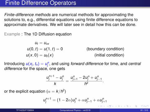
Finite-difference methods are numerical methods for approximating thesolutions to, e.g., differential equations using finite difference equations toapproximate derivatives. We will later see in detail how this can be done.
Example : The 1D Diffusion equation
ut = uxx
u(0, t) = u(1, t) = 0 (boundary condition)u(x ,0) = u0(x) (initial condition)
Introducing u(xj , tn) = unj , and using forward difference for time, and central
difference for the space, one gets
un+1j − un
j
k=
unj+1 − 2un
j + unj−1
h2 .
or the explicit equation (α = k/h2)
un+1j = (1− 2α)un
j + αunj−1 + αun
j+1
TFY4235/FYS8904 Computational Physics – ver2018 81 / 515
Forwards difference
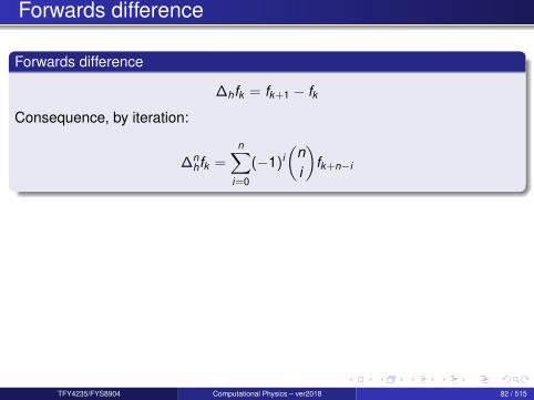
Forwards difference
∆hfk = fk+1 − fk
Consequence, by iteration:
∆nhfk =
n∑i=0
(−1)i(
ni
)fk+n−i
TFY4235/FYS8904 Computational Physics – ver2018 82 / 515
Backwards difference
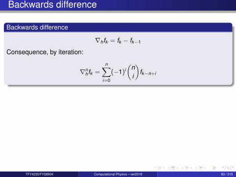
Backwards difference
∇hfk = fk − fk−1
Consequence, by iteration:
∇nhfk =
n∑i=0
(−1)i(
ni
)fk−n+i
TFY4235/FYS8904 Computational Physics – ver2018 83 / 515

Central difference
Central difference
δhfk = fk+1/2 − fk−1/2
Consequence, by iteration:
δnh fk =
n∑i=0
(−1)i(
ni
)fk−n/2+i
But fn/2 is unknown for n odd! We introduce the central average.
Central average
µhfk =12
(fk+1/2 + fk−1/2)
Substitute all odd central differences by central average of centraldifferences:
δhfk = fk+1/2 − fk−1/2 → µhδhfk =12
(fk+1 − fk−1)
TFY4235/FYS8904 Computational Physics – ver2018 84 / 515

Interpolation schemes
How to get as closely as possible to f (x) for any x given f (xk ) = fk ?
We define:u =
x − xk
hand: (
ul
)=
u(u − 1) · · · (u − l + 1)
l!
Be careful, since u is not necessarily an integer here!
TFY4235/FYS8904 Computational Physics – ver2018 85 / 515
Lagrange interpolation
Task : Given a set of N points, (xn, yn)Nn=1, and we want to find an
interpolating function for these points.
Lagrange interpolation is centered around constructing an interpolatingpolynomial P(x) of order ≤ (N − 1) that passes through these points.Lagrange interpolating polynomial reads
P(x) =N∑
n=1
Pn(x)
where
Pn(x) = yn
N∏k=1k 6=n
x − xk
xn − xk
TFY4235/FYS8904 Computational Physics – ver2018 86 / 515

Lagrange interpolation
TFY4235/FYS8904 Computational Physics – ver2018 87 / 515
Splines
The term “spline” is used to refer to a wide class of functions that areused in applications requiring data interpolation and/or smoothingSpline interpolation is a form of interpolation where the interpolant is aspecial type of piecewise polynomial called a splineThe data may be either one-dimensional or multi-dimensional
The splines are often chosen to be of a type that render derivativescontinuous
For details see https://en.wikipedia.org/wiki/Spline_(mathematics)
TFY4235/FYS8904 Computational Physics – ver2018 88 / 515

Newton-Gregory forward interpolation scheme
Newton-Gregory forward interpolation scheme
Fm(x) = fk +m∑
l=1
(ul
)∆l
hfk +O(hm+1)
Fm is a polynomial of order m that passes through m tabulated points(xk+i , fk+1), i ∈ J0; m − 1K
Here Fm(x) represents a mth order polynomial approximation to f (x) for anycoordinate x , i.e. Fm(x) ≈ f (x)!
TFY4235/FYS8904 Computational Physics – ver2018 89 / 515
Newton-Gregory forward interpolation scheme
Example m = 2:
F2(x) = fk +∆hfk
h(x − xk ) +
∆2hfk
2h2 (x − xk )(x − xk+1) +O(h3)
= fk +1h
(fk+1 − fk )(x − xk )
+1
2h2 (fk+2 − 2fk+1 + fk )(x − xk )(x − xk+1) +O(h3)
In particular:
F2(xk ) = fkF2(xk+1) = fk+1
F2(xk+2) = fk+2
TFY4235/FYS8904 Computational Physics – ver2018 90 / 515
Newton-Gregory backward interpolation scheme
Newton-Gregory backward interpolation scheme
Fm(x) = fk +m∑
l=1
(u + l − 1
l
)∇l
hfk +O(hm+1)
Example m = 2:
F2(x) = fk +∇hfk
h(x − xk ) +
∇2hfk
2h2 (x − xk )(x − xk−1) +O(h3)
TFY4235/FYS8904 Computational Physics – ver2018 91 / 515

Stirling interpolation scheme
Stirling interpolation scheme
F2n(x) = fk +n∑
l=1
(u + l − 1
2l − 1
)(µhδ
2l−1h fk +
u2lδ2l
h fk)
+O(h2n+1)
Example n = 1:
F2(x) = fk +µhδhfk
h(x − xk ) +
δ2h fk
2h2 (x − xk )2 +O(h3)
This is the parabolic Stirling formula.
TFY4235/FYS8904 Computational Physics – ver2018 92 / 515

Difference quotients
It can be shown that
ddu
(ul
)=
(ul
) l−1∑i=0
1u − i
d2
du2
(ul
)=
0 if l = 1(u
l
)∑l−1i=0∑l−1
j=01
(u−i)(u−j) if l ≥ 2
These results will be useful when taking the derivatives of theNewton-Gregory schemes as will be done now!
TFY4235/FYS8904 Computational Physics – ver2018 93 / 515
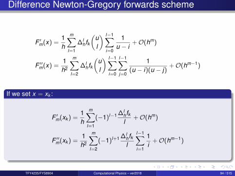
Difference Newton-Gregory forwards scheme
F ′m(x) =1h
m∑l=1
∆lhfk
(ul
) l−1∑i=0
1u − i
+O(hm)
F ′′m(x) =1h2
m∑l=2
∆lhfk
(ul
) l−1∑i=0
l−1∑j=0
1(u − i)(u − j)
+O(hm−1)
If we set x = xk :
F ′m(xk ) =1h
m∑l=1
(−1)l−1 ∆lhfkl
+O(hm)
F ′′m(xk ) =1h2
m∑l=2
(−1)l+1 ∆lhfkl
l−1∑i=1
1i
+O(hm−1)
TFY4235/FYS8904 Computational Physics – ver2018 94 / 515
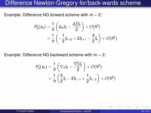
Difference Newton-Gregory for/back-wards scheme
Example: Difference NG forward scheme with m = 2:
F ′2(xk ) =1h
(∆hfk −
∆2hfk2
)+O(h2)
=1h
(−1
2fk+2 + 2fk+1 −
32
fk
)+O(h2)
Example: Difference NG backward scheme with m = 2:
F ′2(xk ) =1h
(∇hfk −
∇2hfk2
)+O(h2)
=1h
(32
fk − 2fk−1 +12
fk−2
)+O(h2)
TFY4235/FYS8904 Computational Physics – ver2018 95 / 515

Differential Stirling formula
It can be shown that
F ′2n(xk ) =1h
(µhδhfk −
16µhδ
3h fk +
130µhδ
5h fk −
1140
µhδ7h fk + · · ·
)+O(h2n)
F ′′2n(xk ) =1h2
(δ2
h fk −1
12δ4
h fk +190δ6
h fk −1
560δ8
h fk + · · ·)
+O(h2n)
Note: in the DNGF and DNGB schemes, the error increases for each neworder of derivation. This does not happen in the DST scheme!
TFY4235/FYS8904 Computational Physics – ver2018 96 / 515

Differential Stirling formula
Example n = 1:
1st derivative
F ′2(xk ) =1hµhδhfk +O(h2)
=1
2h(fk+1 − fk−1) +O(h2)
2nd derivative
F ′′2 (xk ) =δ2
h fkh2 +O(h2)
=1h2 (fk+1 − 2fk + fk−1) +O(h2)
Note: these results are the “standard” central difference approximations forthe 1st and 2nd derivatives
TFY4235/FYS8904 Computational Physics – ver2018 97 / 515

Why does it work so well?
Graphical representation (to come).
TFY4235/FYS8904 Computational Physics – ver2018 98 / 515
Section 4
Linear algebra
TFY4235/FYS8904 Computational Physics – ver2018 99 / 515

Outline I
1 Introduction
2 Number representation and numerical precision
3 Finite differences and interpolation
4 Linear algebraDirect methodsIterative methodsSingular value decomposition
5 How to install libraries on a Linux system
6 Eigenvalue problems
7 Spectral methods
TFY4235/FYS8904 Computational Physics – ver2018 100 / 515

Outline II8 Numerical integration
9 Random numbers
10 Ordinary differential equations
11 Partial differential equations
12 Optimization
TFY4235/FYS8904 Computational Physics – ver2018 101 / 515
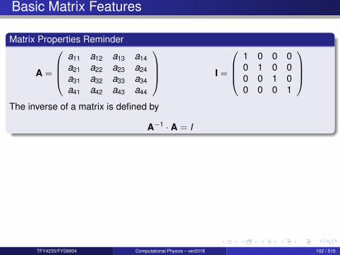
Basic Matrix Features
Matrix Properties Reminder
A =
a11 a12 a13 a14a21 a22 a23 a24a31 a32 a33 a34a41 a42 a43 a44
I =
1 0 0 00 1 0 00 0 1 00 0 0 1
The inverse of a matrix is defined by
A−1 · A = I
TFY4235/FYS8904 Computational Physics – ver2018 102 / 515
Basic Matrix Features
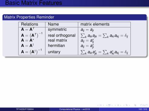
Matrix Properties Reminder
Relations Name matrix elementsA = AT symmetric aij = aji
A =(AT)−1
real orthogonal∑
k aik ajk =∑
k akiakj = δijA = A∗ real matrix aij = a∗ijA = A† hermitian aij = a∗jiA =
(A†)−1 unitary
∑k aik a∗jk =
∑k a∗kiakj = δij
TFY4235/FYS8904 Computational Physics – ver2018 103 / 515
Some famous Matrices
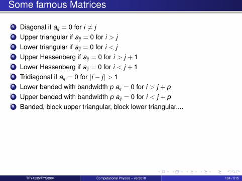
1 Diagonal if aij = 0 for i 6= j2 Upper triangular if aij = 0 for i > j3 Lower triangular if aij = 0 for i < j4 Upper Hessenberg if aij = 0 for i > j + 15 Lower Hessenberg if aij = 0 for i < j + 16 Tridiagonal if aij = 0 for |i − j | > 17 Lower banded with bandwidth p aij = 0 for i > j + p8 Upper banded with bandwidth p aij = 0 for i < j + p9 Banded, block upper triangular, block lower triangular....
TFY4235/FYS8904 Computational Physics – ver2018 104 / 515

Basic Matrix Features
Some Equivalent Statements
For an N × N matrix A the following properties are all equivalent1 If the inverse of A exists, A is nonsingular.2 The equation Ax = 0 implies x = 0.3 The rows of A form a basis of RN .4 The columns of A form a basis of RN .5 A is a product of elementary matrices.6 0 is not eigenvalue of A.
TFY4235/FYS8904 Computational Physics – ver2018 105 / 515

Important Mathematical Operations
The basic matrix operations that we will deal with are addition and subtraction
A = B± C =⇒ aij = bij ± cij ,
scalar-matrix multiplicationA = γB =⇒ aij = γbij ,
vector-matrix multiplication
y = Ax =⇒ yi =n∑
j=1
aijxj ,
matrix-matrix multiplication
A = BC =⇒ aij =n∑
k=1
bik ckj ,
and transpositionA = BT =⇒ aij = bji
TFY4235/FYS8904 Computational Physics – ver2018 106 / 515
Important Mathematical Operations
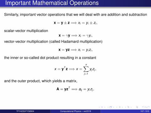
Similarly, important vector operations that we will deal with are addition and subtraction
x = y± z =⇒ xi = yi ± zi ,
scalar-vector multiplicationx = γy =⇒ xi = γyi ,
vector-vector multiplication (called Hadamard multiplication)
x = yz =⇒ xi = yizi ,
the inner or so-called dot product resulting in a constant
x = yT z =⇒ x =n∑
j=1
yjzj ,
and the outer product, which yields a matrix,
A = yzT =⇒ aij = yizj ,
TFY4235/FYS8904 Computational Physics – ver2018 107 / 515

Some notations before starting!
We will denote matrices and vectors by capital letters, and theircomponents by lowercase letters. Example: the matrix A, its element aij .MM,N(R): set of real matrices of size M × N.IN = 1MN (R) the identity matrix.
AT the transpose of the matrix A.GLN(R): general linear group of matrices i.e. set of invertible realmatrices of size N.ON(R): orthogonal group i.e. M ∈ GLN(R),MT M = MMT = INSp(A): spectrum of A, i.e. the set of eigenvalues of A.ker(A): kernel of A, i.e. ker(A) =
v ∈ RN |Av = 0
TFY4235/FYS8904 Computational Physics – ver2018 108 / 515
Linear algebra
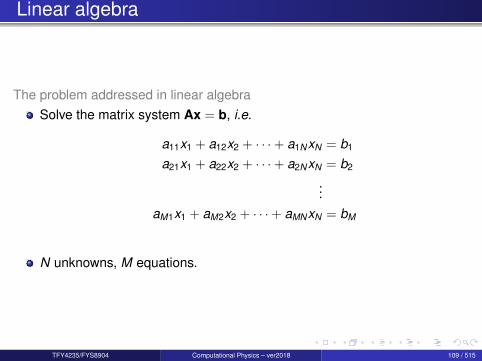
The problem addressed in linear algebraSolve the matrix system Ax = b, i.e.
a11x1 + a12x2 + · · ·+ a1NxN = b1
a21x1 + a22x2 + · · ·+ a2NxN = b2
...aM1x1 + aM2x2 + · · ·+ aMNxN = bM
N unknowns, M equations.
TFY4235/FYS8904 Computational Physics – ver2018 109 / 515

Linear algebra
Three possibilities:If N = M, two possible situations:
a unique solution exists and is given by x = A−1BSome of the equations are linear combinations of others
A is a singular matrix⇒ Degenerate problem.
For a degenerate problem the matrix A is singular i.e. cannot be inverted (inthe normal sense). The solution of Ax = b then consists of a particularsolution xp plus any linear combinations of zero-vectors x0
i such thatAx0
i = 0.
x = xp +D∑
i=1
cix0i
D = dim (ker(A)) The particular solution xp can be found by the so-called
Moore-Pendose pseudoinverse, A+, also know as the generalized inverse.The pseudoinverse always exists.
TFY4235/FYS8904 Computational Physics – ver2018 110 / 515
Linear algebra
If N > M, the equation set is also degenerateIf N < M, the system is overdetermined and probably no solution exists.
This is typically caused by the physical assumptions underlying theequations not being compatible. However, it is still possible to find a bestsolution given the circumstances.
TFY4235/FYS8904 Computational Physics – ver2018 111 / 515

Linear algebra
We now assume: A ∈ GLN(R) or A ∈ GLN(C) (i.e. M = N and A−1 exists).
Two classes of solversDirect solversIterative solvers
When to use a Direct or an Iterative method to solve Ax = b?
Direct methodswill always find the solutiontypically used for dense matricesmatrix inversion takes longLapack useful
Iterative methodssolution not necessarily found(no convergence)typically used for sparsematricespreconditioning usefulcan be fast
TFY4235/FYS8904 Computational Physics – ver2018 112 / 515
Linear algebra
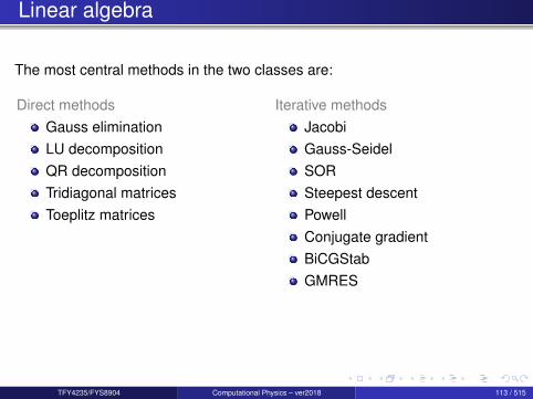
The most central methods in the two classes are:
Direct methodsGauss eliminationLU decompositionQR decompositionTridiagonal matricesToeplitz matrices
Iterative methodsJacobiGauss-SeidelSORSteepest descentPowellConjugate gradientBiCGStabGMRES
TFY4235/FYS8904 Computational Physics – ver2018 113 / 515
Gauss eliminationDirect methods
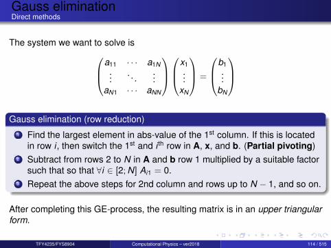
The system we want to solve isa11 · · · a1N...
. . ....
aN1 · · · aNN
x1
...xN
=
b1...
bN
Gauss elimination (row reduction)
1 Find the largest element in abs-value of the 1st column. If this is locatedin row i , then switch the 1st and i th row in A, x, and b. (Partial pivoting)
2 Subtract from rows 2 to N in A and b row 1 multiplied by a suitable factorsuch that so that ∀i ∈ [2; N] Ai1 = 0.
3 Repeat the above steps for 2nd column and rows up to N − 1, and so on.
After completing this GE-process, the resulting matrix is in an upper triangularform.
TFY4235/FYS8904 Computational Physics – ver2018 114 / 515
Gauss eliminationDirect methods
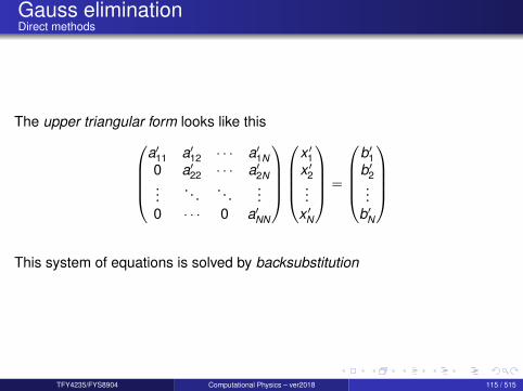
The upper triangular form looks like thisa′11 a′12 · · · a′1N0 a′22 · · · a′2N...
. . . . . ....
0 · · · 0 a′NN
x ′1x ′2...
x ′N
=
b′1b′2...
b′N
This system of equations is solved by backsubstitution
TFY4235/FYS8904 Computational Physics – ver2018 115 / 515

Gauss eliminationDirect methods
Backsubstitution a′11 a′12 · · · a′1N0 a′22 · · · a′2N...
. . . . . ....
0 · · · 0 a′NN
x ′1x ′2...
x ′N
=
b′1b′2...
b′N
Solve the last equation first, then the next-to-last, and so on. . .
x ′N =1
a′NNb′N
x ′N−1 =1
a′N−1 N−1
(b′N−1 − a′N−1 Nx ′N
)...
x ′i =1
a′i i
b′i −N∑
j=i+1
a′i jx′j
TFY4235/FYS8904 Computational Physics – ver2018 116 / 515
LU decompositionDirect methods
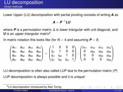
Lower Upper (LU) decomposition with partial pivoting consists of writing A as
A = P−1LU
where P is a permutation matrix; L is lower triangular with unit diagonal, andU is an upper triangular matrix6
In matrix notation this looks like (for N = 4 and assuming P = I)a11 a12 a13 a14a21 a22 a23 a24a31 a32 a33 a34a41 a42 a43 a44
=
1 0 0 0l21 1 0 0l31 l32 1 0l41 l42 l43 1
·
u11 u12 u13 u140 u22 u23 u240 0 u33 u340 0 0 u44
LU decomposition is often also called LUP due to the permutation matrix (P)
LUP decomposition is always possible and it is unique!
6LU decomposition introduced by Alan Turing.TFY4235/FYS8904 Computational Physics – ver2018 117 / 515
LU decompositionDirect methods
LU decomposition can be viewed as the matrix form of Gaussian elimination.
Several algorithms exist for performing LU decomposition
Crout and LUP algorithmsDoolittle algorithmClosed formula
Numerical complexity of the LU decomposition
LU decomposition : 2N3/3forward and backward substitution for solving a linear system: ∝ N2
TFY4235/FYS8904 Computational Physics – ver2018 118 / 515
LU decompositionDirect methods
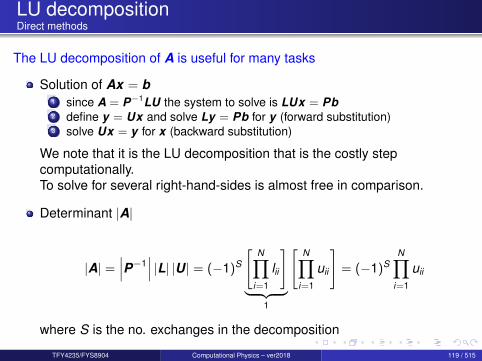
The LU decomposition of A is useful for many tasks
Solution of Ax = b1 since A = P−1LU the system to solve is LUx = Pb2 define y = Ux and solve Ly = Pb for y (forward substitution)3 solve Ux = y for x (backward substitution)
We note that it is the LU decomposition that is the costly stepcomputationally.To solve for several right-hand-sides is almost free in comparison.
Determinant |A|
|A| =∣∣∣P−1
∣∣∣ |L| |U| = (−1)S
[N∏
i=1
lii
]︸ ︷︷ ︸
1
[N∏
i=1
uii
]= (−1)S
N∏i=1
uii
where S is the no. exchanges in the decomposition
TFY4235/FYS8904 Computational Physics – ver2018 119 / 515

LU decompositionDirect methods
Inverse matrix A−1
Solve the systems
Axn = bn forn = 1,2, . . . ,N
with bn zero everywhere, except at row n where it has value 1. Theinverse is then
A−1 = [x1,x2, . . . ,xN ]
In practice this is solved as the matrix system AX = I so that X = A−1
TFY4235/FYS8904 Computational Physics – ver2018 120 / 515

LU decompositionDirect methods
Recommendation: Dense matrix solverLU decomposition (or LU factorization) is the workhorse for solving densematrix systems, finding determinants, and directly obtaining the matrixinverse.
As a general advice, use the LU decomposition for dense matrices.
LAPACKDo not implement the LU decomposition yourself, use the high performancelibrary LAPACK (which depend on BLAS)!You simply can not beat an optimized version of this library!
LAPACK routines (LAPACK95 equivalents: la_getrs / la_getrf )solve system (using LU decomp.) : sgetrs,dgetrs,cgetrs,zgetrsLU factorization : sgetrf,dgetrf,cgetrf,zgetrf
TFY4235/FYS8904 Computational Physics – ver2018 121 / 515

QR decomposition
A general rectangular M-by-N matrix A has a QR decomposition into theproduct of an orthogonal M-by-M square matrix Q (where QT Q = I) and anM-by-N right-triangular (upper-triangular) matrix R,
A = QR
Usage
solving Ax = b by back-substitutionto compute an orthonormal basis for a set of vectors
The first N columns of Q form an orthonormal basis for the range of A,rang(A), when A has full column rank.
TFY4235/FYS8904 Computational Physics – ver2018 122 / 515
Important Matrix and vector handling packages
LAPACK — Linear Algebra Packagehttp://www.netlib.org
The library provides routines for solving systems of linear equations andlinear least squares, eigenvalue problems, and singular valuedecomposition.routines to handle both real and complex matrices in both single and doubleprecision.originally written in FORTRAN 77, but moved to Fortran 90 from version 3.2(2008)ScaLAPACK: Parallel (MPI) versionsource code freely availableFortran and C/C++ versions are availableLAPACK is based on the older LINPACK and EISPACK
LAPACK95 (for Fortran useres)Generic and convenient (modern) Fortran interface to LAPACKSee: www.netlib.org/lapack95/
TFY4235/FYS8904 Computational Physics – ver2018 123 / 515
Important Matrix and vector handling packages
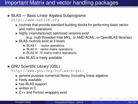
BLAS — Basic Linear Algebra Subprogramshttp://www.netlib.org
routines that provide standard building blocks for performing basic vectorand matrix operationshighly (manufactured) optimized versions exist
(e.g. multi-threaded Intel MKL, or AMD ACML, or OpenBLAS libraries)BLAS routines exist at 3 levels
BLAS I : vector operationsBLAS II : vector-matrix operationsBLAS III : III matrix-matrix operations.
also BLAS is freely available
GNU Scientific Library (GSL)http://www.gnu.org/software/gsl/
general purpose numerical library (including linear algebra)freely availablehas BLAS supportwritten in CC++ and Fortran wrappers exist
TFY4235/FYS8904 Computational Physics – ver2018 124 / 515

Important Matrix and vector handling packages
Armadillo: C++ linear algebra libraryhttp://arma.sourceforge.net/
optional integration with LAPACKsyntax (API) is deliberately similar to Matlablibrary is open-source software
For C++ users, Armadillo is a useful tool!
TFY4235/FYS8904 Computational Physics – ver2018 125 / 515
Important Matrix and vector handling packagesArmadillo, recommended!!
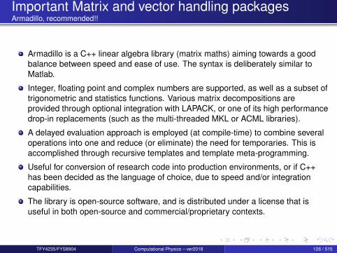
Armadillo is a C++ linear algebra library (matrix maths) aiming towards a goodbalance between speed and ease of use. The syntax is deliberately similar toMatlab.
Integer, floating point and complex numbers are supported, as well as a subset oftrigonometric and statistics functions. Various matrix decompositions areprovided through optional integration with LAPACK, or one of its high performancedrop-in replacements (such as the multi-threaded MKL or ACML libraries).
A delayed evaluation approach is employed (at compile-time) to combine severaloperations into one and reduce (or eliminate) the need for temporaries. This isaccomplished through recursive templates and template meta-programming.
Useful for conversion of research code into production environments, or if C++has been decided as the language of choice, due to speed and/or integrationcapabilities.
The library is open-source software, and is distributed under a license that isuseful in both open-source and commercial/proprietary contexts.
TFY4235/FYS8904 Computational Physics – ver2018 126 / 515
Important Matrix and vector handling packagesUsing libraries
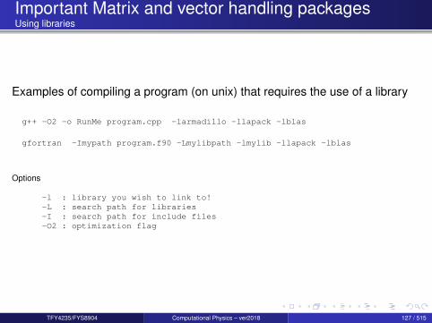
Examples of compiling a program (on unix) that requires the use of a library
g++ -O2 -o RunMe program.cpp -larmadillo -llapack -lblas
gfortran -Imypath program.f90 -Lmylibpath -lmylib -llapack -lblas
Options
-l : library you wish to link to!-L : search path for libraries-I : search path for include files-O2 : optimization flag
TFY4235/FYS8904 Computational Physics – ver2018 127 / 515
Important Matrix and vector handling packagesArmadillo, simple examples
#include <iostream>#include "armadillo"using namespace arma;using namespace std;
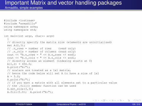
int main(int argc, char** argv)// directly specify the matrix size (elements are uninitialised)mat A(2,3);// .n_rows = number of rows (read only)// .n_cols = number of columns (read only)cout << "A.n_rows = " << A.n_rows << endl;cout << "A.n_cols = " << A.n_cols << endl;// directly access an element (indexing starts at 0)A(1,2) = 456.0;A.print("A:");// scalars are treated as a 1x1 matrix,// hence the code below will set A to have a size of 1x1A = 5.0;A.print("A:");// if you want a matrix with all elements set to a particular value// the .fill() member function can be usedA.set_size(3,3);A.fill(5.0); A.print("A:");
TFY4235/FYS8904 Computational Physics – ver2018 128 / 515

Important Matrix and vector handling packagesArmadillo, simple examples
mat B;
// endr indicates "end of row"B << 0.555950 << 0.274690 << 0.540605 << 0.798938 << endr
<< 0.108929 << 0.830123 << 0.891726 << 0.895283 << endr<< 0.948014 << 0.973234 << 0.216504 << 0.883152 << endr<< 0.023787 << 0.675382 << 0.231751 << 0.450332 << endr;
// print to the cout stream// with an optional string before the contents of the matrixB.print("B:");
// the << operator can also be used to print the matrix// to an arbitrary stream (cout in this case)cout << "B:" << endl << B << endl;// save to diskB.save("B.txt", raw_ascii);// load from diskmat C;C.load("B.txt");C += 2.0 * B;C.print("C:");
TFY4235/FYS8904 Computational Physics – ver2018 129 / 515
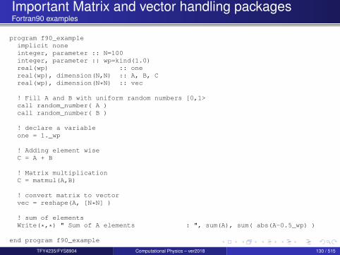
Important Matrix and vector handling packagesFortran90 examples
program f90_exampleimplicit noneinteger, parameter :: N=100integer, parameter :: wp=kind(1.0)real(wp) :: onereal(wp), dimension(N,N) :: A, B, Creal(wp), dimension(N*N) :: vec
! Fill A and B with uniform random numbers [0,1>call random_number( A )call random_number( B )
! declare a variableone = 1._wp
! Adding element wiseC = A + B
! Matrix multiplicationC = matmul(A,B)
! convert matrix to vectorvec = reshape(A, [N*N] )
! sum of elementsWrite(*,*) " Sum of A elements : ", sum(A), sum( abs(A-0.5_wp) )
end program f90_example
TFY4235/FYS8904 Computational Physics – ver2018 130 / 515
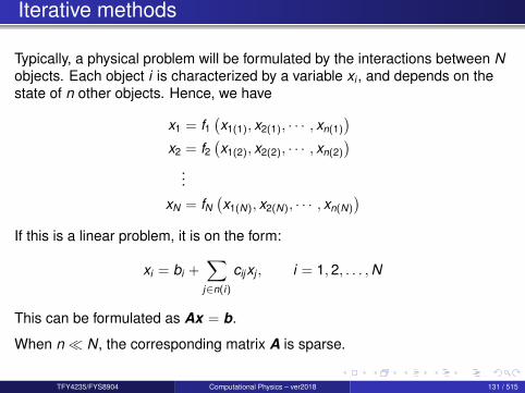
Iterative methods
Typically, a physical problem will be formulated by the interactions between Nobjects. Each object i is characterized by a variable xi , and depends on thestate of n other objects. Hence, we have
x1 = f1(x1(1), x2(1), · · · , xn(1)
)x2 = f2
(x1(2), x2(2), · · · , xn(2)
)...
xN = fN(x1(N), x2(N), · · · , xn(N)
)If this is a linear problem, it is on the form:
xi = bi +∑
j∈n(i)
cijxj , i = 1,2, . . . ,N
This can be formulated as Ax = b.
When n N, the corresponding matrix A is sparse.
TFY4235/FYS8904 Computational Physics – ver2018 131 / 515

Iterative methodsGeneral comments
Objective of iterative methods:to construct a sequence x (k)∞k=1, so that x (k) converges to a fixedvector x?, where x? is the solution of the problem (e.g. a linear system)
General iteration ideaSay that we want to solve the equations
g(x) = 0,
and the equation x = f (x) has the same solution as it, then construct
x (k+1) = f (x (k)).
If x (k) → x?, then x? = f (x?), and the root of g(x) = 0 is obtained.
When this strategy is applied to Ax = b, the functions f (·) and g(·) are linearoperators.
TFY4235/FYS8904 Computational Physics – ver2018 132 / 515
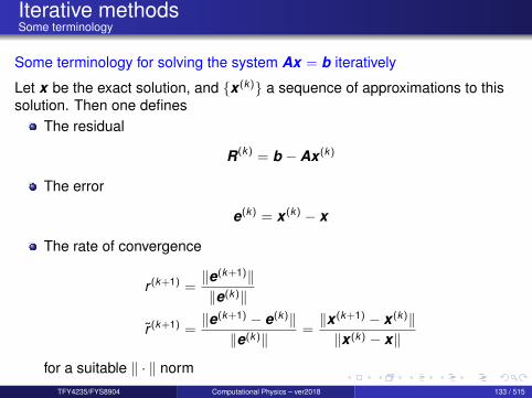
Iterative methodsSome terminology
Some terminology for solving the system Ax = b iteratively
Let x be the exact solution, and x (k) a sequence of approximations to thissolution. Then one defines
The residual
R(k) = b − Ax (k)
The error
e(k) = x (k) − x
The rate of convergence
r (k+1) =‖e(k+1)‖‖e(k)‖
r (k+1) =‖e(k+1) − e(k)‖‖e(k)‖ =
‖x (k+1) − x (k)‖‖x (k) − x‖
for a suitable ‖ · ‖ normTFY4235/FYS8904 Computational Physics – ver2018 133 / 515

Iterative methods
Basic idea behind iterative methods for solving Ax = b
Start with an initial guess for the solution x (0).Obtain x (k+1) from the knowledge of x (k) for k = 0,1, . . .If ‖Ax (k) − b‖ −−−→
k→∞0 then x (k) −−−→
k→∞x ; the solution of Ax = b is found
The two main classes of iterative methods (for linear systems) are:
Stationary iterative methods
JacobiGauss-SeidelSOR
Krylov subspace methodsConjugate gradientBiCGStabGMRESSteepest descentPowell
TFY4235/FYS8904 Computational Physics – ver2018 134 / 515

Jacobi algorithm
The Jacobi iteration method is one of the oldest and simplest methods
Decompose the matrix A as follows
A = D + L + U,
whereD is diagonalL and U are strict lower and upper triangular matrices
D =
a11 0 · · · 00 a22 · · · 0...
.... . .
...0 0 · · · aNN
, L =
0 0 · · · 0
a21 0 · · · 0...
.... . .
...aN1 aN2 · · · 0
, U =
0 a12 · · · a1N
0 0 · · · a2N...
.... . .
...0 0 · · · 0
.
TFY4235/FYS8904 Computational Physics – ver2018 135 / 515
Jacobi algorithm
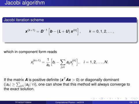
Jacobi iteration scheme
x (k+1) = D−1[b − (L + U) x (k)
], k = 0,1,2, . . . ,
which in component form reads
x (k+1)i =
1aii
[bi −
∑j 6=i
aijx(k)j
], i = 1,2, . . . ,N.
If the matrix A is positive definite (xT Ax > 0) or diagonally dominant(|aii | ≥
∑j 6=i |aij | ∀i), one can show that this method will always converge to
the exact solution.
TFY4235/FYS8904 Computational Physics – ver2018 136 / 515
Other iterative methods
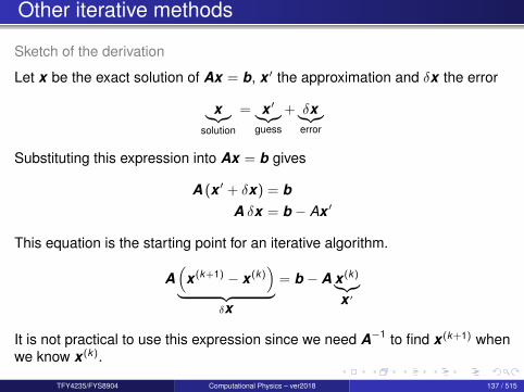
Sketch of the derivation
Let x be the exact solution of Ax = b, x ′ the approximation and δx the error
x︸︷︷︸solution
= x ′︸︷︷︸guess
+ δx︸︷︷︸error
Substituting this expression into Ax = b gives
A (x ′ + δx) = bA δx = b − Ax ′
This equation is the starting point for an iterative algorithm.
A(
x (k+1) − x (k))
︸ ︷︷ ︸δx
= b − A x (k)︸︷︷︸x ′
It is not practical to use this expression since we need A−1 to find x (k+1) whenwe know x (k).
TFY4235/FYS8904 Computational Physics – ver2018 137 / 515
Other iterative methods
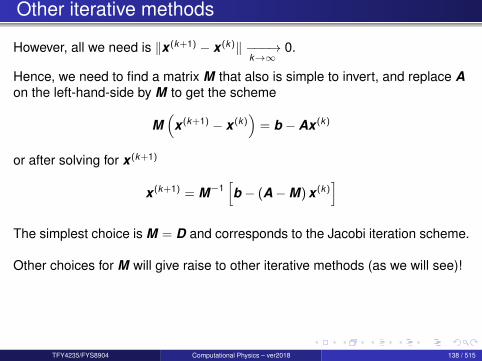
However, all we need is ‖x (k+1) − x (k)‖ −−−→k→∞
0.
Hence, we need to find a matrix M that also is simple to invert, and replace Aon the left-hand-side by M to get the scheme
M(
x (k+1) − x (k))
= b − Ax (k)
or after solving for x (k+1)
x (k+1) = M−1[b − (A−M) x (k)
]The simplest choice is M = D and corresponds to the Jacobi iteration scheme.
Other choices for M will give raise to other iterative methods (as we will see)!
TFY4235/FYS8904 Computational Physics – ver2018 138 / 515

Other iterative methods
Spectral radiusThe spectral radius of a matrix A is defined as
ρ(A) = maxλ|λ(A)|
Theorem (Spectral radius and iterative convergence)If A ∈ Rn, then
limk→∞
Ak = 0⇐⇒ ρ(A) < 1
TFY4235/FYS8904 Computational Physics – ver2018 139 / 515
Other iterative methods
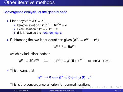
Convergence analysis for the general case
Linear system Ax = bIterative solution : x (k+1) = Bx (k) + cExact solution : x? = Bx? + cB is known as the iteration matrix
Subtracting the two latter equations gives (e(k) = x (k) − x?)
e(k+1) = Be(k)
which by induction leads to
e(k) = Bk e(0) ⇐⇒ ‖e(k)‖ = ρk (B)‖e(0)‖ (when k →∞ )
This means that
e(k) → 0⇐⇒ Bk → 0⇐⇒ ρ(B) < 1
This is the convergence criterion for general iterations.
TFY4235/FYS8904 Computational Physics – ver2018 140 / 515

Gauss-Seidel relaxation
Jacobi method
x (k+1)1 =(b1 − a12x (k)
2 − a13x (k)3 − a14x (k)
4 )/a11
x (k+1)2 =(b2 − a21x (k)
1 − a23x (k)3 − a24x (k)
4 )/a22
x (k+1)3 =(b3 − a31x (k)
1 − a32x (k)2 − a34x (k)
4 )/a33
x (k+1)4 =(b4 − a41x (k)
1 − a42x (k)2 − a43x (k)
3 )/a44,
Idea: Update each component of x (k)i sequentially with the most updated
information available
x (k+1)1 = (b1 − a12x (k)
2 − a13x (k)3 − a14x (k)
4 )/a11
x (k+1)2 = (b2 − a21x (k+1)
1 − a23x (k)3 − a24x (k)
4 )/a22
x (k+1)3 = (b3 − a31x (k+1)
1 − a32x (k+1)2 − a34x (k)
4 )/a33
x (k+1)4 = (b4 − a41x (k+1)
1 − a42x (k+1)2 − a43x (k+1)
3 )/a44
This procedure leads to the Gauss-Seidel method and improves normally theconvergence behavior.
TFY4235/FYS8904 Computational Physics – ver2018 141 / 515
Gauss-Seidel relaxation
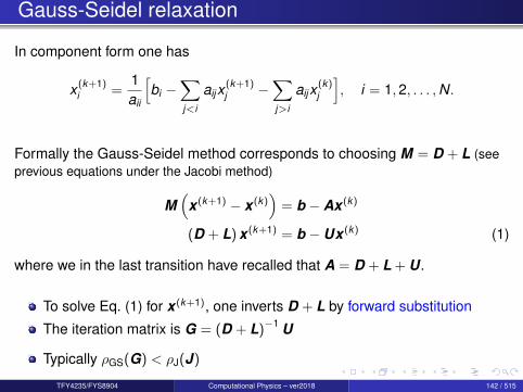
In component form one has
x (k+1)i =
1aii
[bi −
∑j<i
aijx(k+1)j −
∑j>i
aijx(k)j
], i = 1,2, . . . ,N.
Formally the Gauss-Seidel method corresponds to choosing M = D + L (seeprevious equations under the Jacobi method)
M(
x (k+1) − x (k))
= b − Ax (k)
(D + L) x (k+1) = b − Ux (k) (1)
where we in the last transition have recalled that A = D + L + U.
To solve Eq. (1) for x (k+1), one inverts D + L by forward substitution
The iteration matrix is G = (D + L)−1 U
Typically ρGS(G) < ρJ(J)
TFY4235/FYS8904 Computational Physics – ver2018 142 / 515
Gauss-Seidel relaxation
When will we have convergence?:
Both Jacobi and Gauss-Seidel require ρ(M) < 1 to converge, i.e. thespectral radius of the respective iteration matrices is less than one
For instance, this means that both methods converge when the matrix Ais symmetric, positive-definite, or is strictly or irreducibly diagonallydominant.
Both methods sometimes converge even if these conditions are notsatisfied.
TFY4235/FYS8904 Computational Physics – ver2018 143 / 515
Successive Over Relaxation (SOR)
SOR is an efficient algorithm that should be considered.
Idea: x (k+1) is a weighted average of x (k) and x (k+1)GS
x (k+1) = ωx (k+1)GS + (1− ω)x (k) (2)
where ω is the relaxation parameterThe special case ω = 1 corresponds to the Gauss-Seidel methodchoose ω to accelerate the rate of convergence of the SOR method
In terms of components we have
x (k+1)i =
ω
aii
[bi −
∑j<i
aijx(k+1)j −
∑j>i
aijx(k)j
]+ (1− ω)x (k)
i , i = 1,2, . . . ,N.
TFY4235/FYS8904 Computational Physics – ver2018 144 / 515
Successive Over Relaxation (SOR)
The matrix form of the SOR method is obtained from (i = 1,2, . . . ,N)
x (k+1)i =
ω
aii
[bi −
∑j<i
aijx(k+1)j −
∑j>i
aijx(k)j
]+ (1− ω)x (k)
i ,
by multiplying with aii and rearranging to get
aiix(k+1)i + ω
∑j<i
aijx(k+1)j = ωbi − ω
∑j>i
aijx(k)j + aii (1− ω)x (k)
i
which in matrix notation may be expressed as
(D + ωL) x (k+1) = ωb − [ωU + (ω − 1)D] x (k).
This implies that the iteration matrix for the SOR method is
S = − (D + ωL)−1 [ωU + (ω − 1)D] .
Normally one finds
ρ(S) < ρ(G) < ρ(J),
i.e. the SOR method converges faster than the Gauss-Seidel and Jacobimethods
TFY4235/FYS8904 Computational Physics – ver2018 145 / 515

Successive Over Relaxation (SOR)
Question: What value to choose for ω?
The SOR-sequence converges for 0 < ω < 2 [Kahan (1958)]Optimal value for ω
ω =2
1 +√
1− ρ(J)2,
but this value is not known in advance
Frequently, some heuristic estimate is used, such as
ω = 2−O(h)
where h is the mesh spacing of the discretization of the underlyingphysical domain.
TFY4235/FYS8904 Computational Physics – ver2018 146 / 515
Successive Over Relaxation (SOR)
Alternative, motivation for the SOR iteration formula!
Starting from the linear system
Ax = b,
multiplying by ω and adding Dx to both sides of the equation, leads to
(D + ωL) x = ωb − [ωU + (ω − 1)D] x
after some trivial manipulation
This equation is the starting point for an iterative scheme — the SOR method!
TFY4235/FYS8904 Computational Physics – ver2018 147 / 515
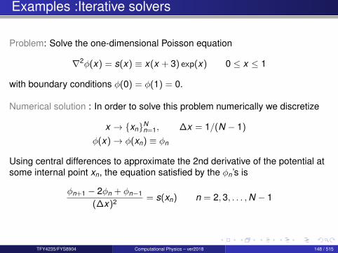
Examples :Iterative solvers
Problem: Solve the one-dimensional Poisson equation
∇2φ(x) = s(x) ≡ x(x + 3) exp(x) 0 ≤ x ≤ 1
with boundary conditions φ(0) = φ(1) = 0.
Numerical solution : In order to solve this problem numerically we discretize
x → xnNn=1, ∆x = 1/(N − 1)
φ(x)→ φ(xn) ≡ φn
Using central differences to approximate the 2nd derivative of the potential atsome internal point xn, the equation satisfied by the φn’s is
φn+1 − 2φn + φn−1
(∆x)2 = s(xn) n = 2,3, . . . ,N − 1
TFY4235/FYS8904 Computational Physics – ver2018 148 / 515

Examples
Defining the vector x = [φ2, φ3, . . . , φN−1]T results in the tridiagonal system
Ax = b,
where
A =
2 −1 0 . . . 0−1 2 −1 . . . 00 −1 2 . . . 0...
......
. . . 00 0 . . . −1 2
b = −(∆x)2
s(x2)s(x3)
...
...s(xN−1)
.
It is this system of equations we will need to solve!
Direct solvers for tridiagonal systems (LAPACK): sgttrs, dgttrs, cgttrs, zgttrs
TFY4235/FYS8904 Computational Physics – ver2018 149 / 515
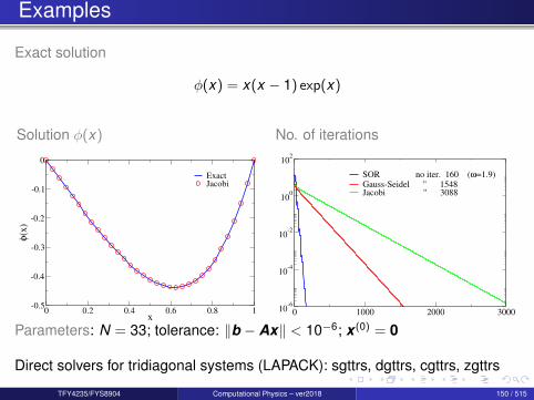
Examples
Exact solution
φ(x) = x(x − 1) exp(x)
Solution φ(x)
0 0.2 0.4 0.6 0.8 1x
-0.5
-0.4
-0.3
-0.2
-0.1
0
φ(x)
ExactJacobi
No. of iterations
0 1000 2000 300010-6
10-4
10-2
100
102
SOR no iter. 160 (ω=1.9)
Gauss-Seidel " 1548Jacobi " 3088
Parameters: N = 33; tolerance: ‖b − Ax‖ < 10−6; x (0) = 0
Direct solvers for tridiagonal systems (LAPACK): sgttrs, dgttrs, cgttrs, zgttrs
TFY4235/FYS8904 Computational Physics – ver2018 150 / 515
Krylov subspace methods
TFY4235/FYS8904 Computational Physics – ver2018 151 / 515
Krylov subspace methods
Krylov subspace methods are also know as conjugate gradient methods!
What is a Krylov space?In linear algebra, the order-r Krylov subspace generated by an N × N matrixA and a vector b of dimension N is the linear subspace spanned by theimages of b under the first r − 1 powers of A (starting from A0 = I), that is
Kr (A,b) = span b,Ab,A2b, . . . ,Ar−1b.
Working principleKrylov subspace methods work by forming a basis of the sequence ofsuccessive matrix powers times the initial residual (the Krylov sequence). Theapproximations to the solution are then formed by minimizing the residual overthe subspace formed.The prototypical method in this class is the conjugate gradient method (CG).Other methods are the generalized minimal residual method (GMRES) andthe biconjugate gradient Stabilized method (BiCGStab).
TFY4235/FYS8904 Computational Physics – ver2018 152 / 515
Steepest descent
Task : Minimize the function f (x i )!
Philosophy of the Steepest decent method
Start at some point x0. As many times as needed, move from point x i to pointx i+1 by minimizing along the line from x i in the direction of the local downhillgradient −∇f (x i )
However, as we will see, this simple strategy is not very efficient, but amodified version of the main idea is!
TFY4235/FYS8904 Computational Physics – ver2018 153 / 515

Steepest descent
The steepest decent strategy applied to the solution of the linear systemAx = b
Assume A to be symmetric and positive definite7.Define the function f (·) — a quadratic form
f (x) =12
xT Ax − x · b, f : RN → R+
=12〈x ,Ax〉 − 〈x ,b〉
f (x) has a minimum when (remember A is symmetric):
∇f (x) = Ax − b = 0
The solution of Ax = b corresponds to the minimum of f .
7That is A is symmetric and xT Ax > 0, or equivalently, all its eigenvalues are positive(∀x ∈M∗N,1, xT Ax > 0 ⇔ Sp(A) ⊂]0; +∞[)
TFY4235/FYS8904 Computational Physics – ver2018 154 / 515

Cauchy steepest descent method
The algorithm1 Choose an initial vector x0.2 If ∇f (xk ) 6= 0 move in the direction of dk = −∇f (xk ).3 Stop at the minimum along direction dk , i.e. solve:
ddαk
f (xk + αk dk ) = 0 =⇒ αk =dk · rk
dTk Adk
[rk = b − Axk ]
4 Define new minimizer : xk+1 = xk + αk dk
5 Let k → k + 1 and repeat the above steps
Comment : the method can be generalized to matrices A that are not symmetric and positive definite. One
simply applies the algorithm to the linear system AT Ax = AT b instead; However, better to use more
sophisticated methods (since AT A is badly conditioned)!
TFY4235/FYS8904 Computational Physics – ver2018 155 / 515
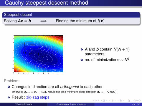
Cauchy steepest descent method
Steepest decent
Solving Ax = b ⇐⇒ Finding the minimum of f (x)
A and b contain N(N + 1)parametersno. of minimizations ∼ N2
Problem:Changes in direction are all orthogonal to each otherotherwise xk+1 = xk + αk dk would not be a minimum along direction dk = −∇f (xk )
Result : zig-zag steps
TFY4235/FYS8904 Computational Physics – ver2018 156 / 515
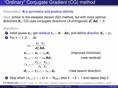
“Ordinary” Conjugate Gradient (CG) method
Assumption: A is symmetric and positive-definite
Idea: similar to the steepest decent (SD) method, but with more optimaldirections dk ; CG uses conjugate directions (A-orthogonal) dT
i Ad j = 0.
Algorithm :1 Initial guess x0; get residual r0 = b − Ax0 and define direction d0 = r0.2 For k = 1,2, . . . do
αk =rk · rk
dTk Adk
xk+1 = xk + αk dk (improved minimizer)rk+1 = rk − αk Adk (new residual)
βk+1 =rk+1 · rk+1
rk · rk
dk+1 = rk+1 + βk+1dk (new search direction)
3 Stop when ‖rk+1‖ < ε or k = Nmax; else k → k + 1 and repeat step 2For details see: http://www.cs.cmu.edu/˜quake-papers/painless-conjugate-gradient.pdf
TFY4235/FYS8904 Computational Physics – ver2018 157 / 515

“Ordinary” Conjugate Gradient (CG) method
CommentsCG completes after N iterations (exact arithmetic’s) [if A is positive-definite]
In practice, set max. no. of interactions to 2N due to roundoff errors
The search directions are built from the residuals
Search directions are orthogonal to previous residuals, i.e. orthogonal tothe (Krylov) space spanned by previous residuals
This means that we will find the minimum of f (x) — the solution to Ax = b— in maximum N iterations
Note: If A = AT is symmetric, but not necessarily positive-definite, theCG method is still found in practice to work well
However, the convergence in N steps is no longer guaranteed (not even intheory)
TFY4235/FYS8904 Computational Physics – ver2018 158 / 515

“Ordinary” Conjugate Gradient (CG) method
The vectors rk and dk satisfy (can be shown)
r i · r j = 0, i < j orthogonalityr i · d j = d i · r j = 0, i < j mutual orthogonality
dTi A · d j = 0, i < j conjugacy
Better name for the method may have been : Conjugate Directions(since the all gradients (or residuals), ∇f (xk ) = −rk , are not conjugate)
TFY4235/FYS8904 Computational Physics – ver2018 159 / 515
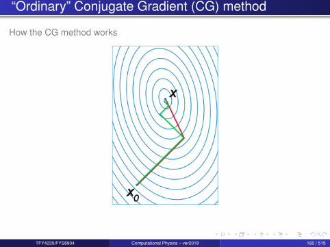
“Ordinary” Conjugate Gradient (CG) method
How the CG method works
TFY4235/FYS8904 Computational Physics – ver2018 160 / 515
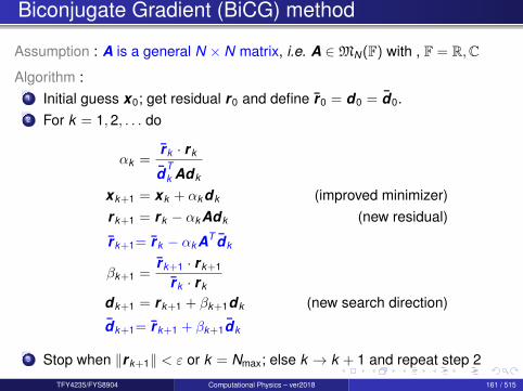
Biconjugate Gradient (BiCG) method
Assumption : A is a general N × N matrix, i.e. A ∈MN(F) with , F = R,C
Algorithm :1 Initial guess x0; get residual r0 and define r0 = d0 = d0.2 For k = 1,2, . . . do
αk =rk · rk
dTk Adk
xk+1 = xk + αk dk (improved minimizer)rk+1 = rk − αk Adk (new residual)
rk+1= rk − αk AT dk
βk+1 =rk+1 · rk+1
rk · rk
dk+1 = rk+1 + βk+1dk (new search direction)
dk+1= rk+1 + βk+1dk
3 Stop when ‖rk+1‖ < ε or k = Nmax; else k → k + 1 and repeat step 2
TFY4235/FYS8904 Computational Physics – ver2018 161 / 515
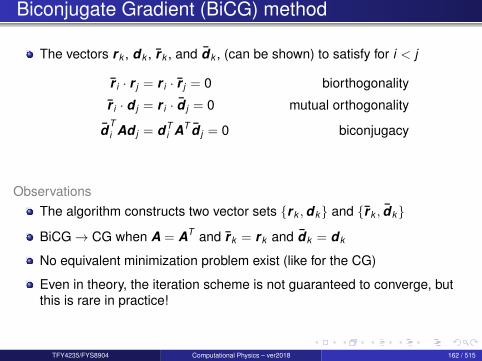
Biconjugate Gradient (BiCG) method
The vectors rk , dk , rk , and dk , (can be shown) to satisfy for i < j
r i · r j = r i · r j = 0 biorthogonality
r i · d j = r i · d j = 0 mutual orthogonality
dTi Ad j = dT
i AT d j = 0 biconjugacy
ObservationsThe algorithm constructs two vector sets rk ,dk and rk , dkBiCG→ CG when A = AT and rk = rk and dk = dk
No equivalent minimization problem exist (like for the CG)
Even in theory, the iteration scheme is not guaranteed to converge, butthis is rare in practice!
TFY4235/FYS8904 Computational Physics – ver2018 162 / 515
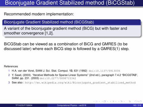
Biconjugate Gradient Stabilized method (BiCGStab)
Recommended modern implementation:
Biconjugate Gradient Stabilized method (BiCGStab)
A variant of the biconjugate gradient method (BiCG) but with faster andsmoother convergence [1,2].
BiCGStab can be viewed as a combination of BiCG and GMRES (to bediscussed later) where each BiCG step is followed by a GMRES(1) step.
References
1 H.A. van der Vorst, SIAM J. Sci. Stat. Comput. 13, 631 (1992) doi:10.1137/0913035
2 Y. Saad, (2003). “Iterative Methods for Sparse Linear Systems” (2nd ed.), paragraph 7.4.2 “BICGSTAB”,SIAM. pp. 231. (2003) doi:10.2277/0898715342
3 See also : http://en.wikipedia.org/wiki/Biconjugate_gradient_stabilized_method
TFY4235/FYS8904 Computational Physics – ver2018 163 / 515
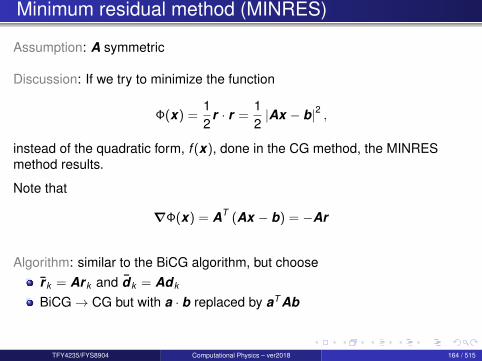
Minimum residual method (MINRES)
Assumption: A symmetric
Discussion: If we try to minimize the function
Φ(x) =12
r · r =12|Ax − b|2 ,
instead of the quadratic form, f (x), done in the CG method, the MINRESmethod results.
Note that
∇Φ(x) = AT (Ax − b) = −Ar
Algorithm: similar to the BiCG algorithm, but chooserk = Ark and dk = Adk
BiCG→ CG but with a · b replaced by aT Ab
TFY4235/FYS8904 Computational Physics – ver2018 164 / 515
Generalized minimum residual method (GMRES)
Assumption : A is a general nonsymmetric matrix
Generalized Minimum Residual method (GMRES)
Generalization and extension of the MINRES to nonsymmetric generalmatrices. The method is fairly robust!
GMRES approximates the exact solution of Ax = b by the vectorxk ∈ Kk (A, r0) that minimizes the Euclidean norm of the residual‖rk‖ = ‖b − Axk‖.Also GMRES should converge to the solution (in theory) after N iterations
The cost of the iterations grows as O(k2), where k is the iteration number
GMRES is therefore often “restarted” after m steps =⇒ GMRES(m)
References1 Y. Saad, “Iterative Methods for Sparse Linear Systems, 2nd edition, Society for Industrial and Applied
Mathematics, 2003.2 See also : http://en.wikipedia.org/wiki/Generalized_minimal_residual_method
TFY4235/FYS8904 Computational Physics – ver2018 165 / 515

Preconditioning
GOAL : Transform the system matrix to a simpler form (closer to the identitymatrix), so that fewer iterations will be needed to find the solution
How can this be done?The system
Ax = b
can be preconditioned with left (PL) and right (PR) precondition matrices as
PLAP−1R PRx = PLb
In general, a good preconditioner should meet the following requirements:The preconditioned system should be easy to solveThe preconditioner should be cheap to construct and apply
Ref: Journal of Computational Physics 182, 418 (2002)
http://www.mathcs.emory.edu/˜benzi/Web_papers/survey.pdf
TFY4235/FYS8904 Computational Physics – ver2018 166 / 515
Preconditioning
Iterative solvers are typically combined with preconditonrs
GOAL : to reduce the condition number of the left or right preconditionedsystem matrix
Instead of solving the original linear system Ax = b, one may solve either theright preconditioned system:
AP−1Px = b
via solving
AP−1y = b
for y and
Px = y
for x ; or the left preconditioned system:
P−1(Ax − b) = 0
both of which give the same solution as the original system as long as thepreconditioning matrix P is nonsingular.
TFY4235/FYS8904 Computational Physics – ver2018 167 / 515
Preconditioning
Examples of preconditioners:
Jacobi (or diagonal)[P = diag(A)]Sparse Approximate InverseIncomplete CholeskyfactorizationIncomplete LU factorization
Successive over-relaxationSymmetric successiveover-relaxationMultigridFourier Acceleration
Which method to use depend on the problem at hand, and the computationalcost of P−1!
Hence, no general best answer exists!
TFY4235/FYS8904 Computational Physics – ver2018 168 / 515
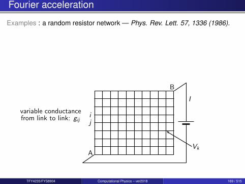
Fourier acceleration
Examples : a random resistor network — Phys. Rev. Lett. 57, 1336 (1986).
A
B
I
ij
variable conductancefrom link to link: gij
Vk
Figure: Resistor network.
TFY4235/FYS8904 Computational Physics – ver2018 169 / 515

Fourier accelerationThe Kirchhoff equations: ∑
j
gij (Vi − Vj ) + Ii = 0
with
Ii =
0 if i 6= A,BI if i = A,B
On matrix formGV + I = 0
A very simple iterative process to solve this equation, is to set
dVdt
= GV + I
Solution of the problem as t →∞
dVdt→ 0
TFY4235/FYS8904 Computational Physics – ver2018 170 / 515
Fourier acceleration
Now, imagine all gij = 1 (they are in general not!) so that we have:∑j
(Vi − Vj ) + Ii = 0
Details to be presented on the backboard!
TFY4235/FYS8904 Computational Physics – ver2018 171 / 515
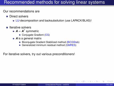
Recommended methods for solving linear systems
Our recommendations are
Direct solversLU-decomposition and backsubsitution (use LAPACK/BLAS)!
Iterative solversA = AT symmetric
Conjugate Gradient (CG)A is a general matrix
Biconjugate Gradient Stabilized method (BiCGStab)Generalized minimum residual method (GMRES)
For iterative solvers, try out various preconditioners!
TFY4235/FYS8904 Computational Physics – ver2018 172 / 515
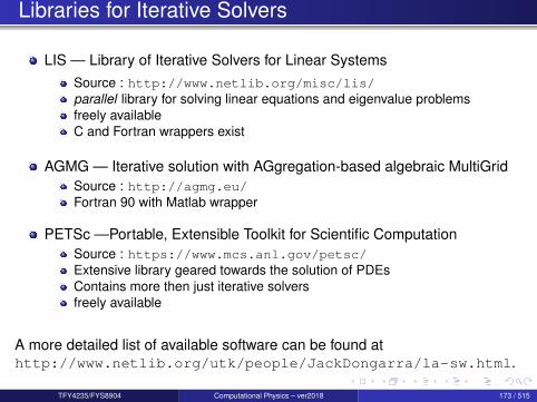
Libraries for Iterative Solvers
LIS — Library of Iterative Solvers for Linear SystemsSource : http://www.netlib.org/misc/lis/parallel library for solving linear equations and eigenvalue problemsfreely availableC and Fortran wrappers exist
AGMG — Iterative solution with AGgregation-based algebraic MultiGridSource : http://agmg.eu/Fortran 90 with Matlab wrapper
PETSc —Portable, Extensible Toolkit for Scientific ComputationSource : https://www.mcs.anl.gov/petsc/Extensive library geared towards the solution of PDEsContains more then just iterative solversfreely available
A more detailed list of available software can be found athttp://www.netlib.org/utk/people/JackDongarra/la-sw.html.
TFY4235/FYS8904 Computational Physics – ver2018 173 / 515
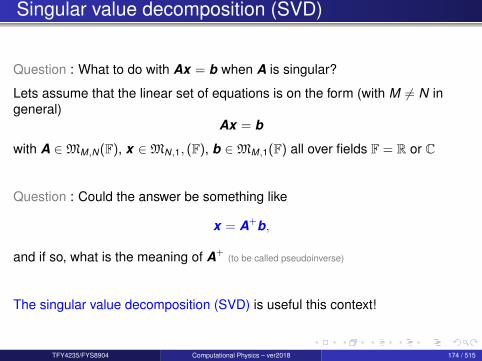
Singular value decomposition (SVD)
Question : What to do with Ax = b when A is singular?
Lets assume that the linear set of equations is on the form (with M 6= N ingeneral)
Ax = b
with A ∈MM,N(F), x ∈MN,1, (F), b ∈MM,1(F) all over fields F = R or C
Question : Could the answer be something like
x = A+b,
and if so, what is the meaning of A+(to be called pseudoinverse)
The singular value decomposition (SVD) is useful this context!
TFY4235/FYS8904 Computational Physics – ver2018 174 / 515

Singular value decomposition (SVD)
Definition: Singular values
Let A ∈ CM×N . A non-negative real number s is a singular value for A iff thereexist unit-vectors u ∈ CM and v ∈ CN such that
Av = su A†u = sv .
The vectors u and v are called left-singular and right-singular vectors for s,respectively.
The singular values of A will be denoted by s1, s2, . . . , smin(M,N), and it iscustomary to list them in decreasing order
s1 ≥ s2 ≥ . . . ≥ smin(M,N)
Here A† denotes the conjugate transpose of A, i.e. A† = (A∗)T
TFY4235/FYS8904 Computational Physics – ver2018 175 / 515
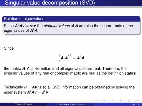
Singular value decomposition (SVD)
Relation to eigenvalues
Since A†Av = s2v the singular values of A are also the square roots of theeigenvalues of A†A.
Since (A†A
)†= A†A
the matrix A†A is Hermitian and all eigenvalues are real. Therefore, thesingular values of any real or complex matrix are real as the definition states!
Technically u = Av/s so all SVD information can be obtained by solving theeigensystem A†Av = s2v .
TFY4235/FYS8904 Computational Physics – ver2018 176 / 515

Singular value decomposition (SVD)
Full SVD decomposition
Decompose a matrix A ∈MM,N(C) into the form
A = U S V †
where
U†U = I (unitary) U ∈ CM×M
V †V = I (unitary) V ∈ CN×N
S = diag(s1, s2, . . . , smin(M,N)) S ∈ RM×N
Here U† denotes the conjugate transpose or adjoint of U.
Note : When A ∈ RM×N , i.e. is a real matrix, U† = UT and V † = V T are realand orthogonal matrices!
TFY4235/FYS8904 Computational Physics – ver2018 177 / 515

Singular value decomposition (SVD)
Warning
Several so-called reduced SVD decompositions exist where not all details ofthe full SVD decomposition are calculated
The Thin SVD (e.g. used by numerical recipes)
A = UN SN V †
where UN ∈ CM×N ; SN ∈ RN×N ; and (as before) V ∈ CN×N .
SoftwareNumerical Recipes calculates the thin SVD
LAPACK calculates the full SVD
Matlab/Octave calculate full SVD
Python (via numpy) can calculate both full and reduced SVDs
TFY4235/FYS8904 Computational Physics – ver2018 178 / 515

Singular value decomposition (SVD)
Comments
SVD is always possible and the decomposition is unique(except for permutations of columns in U and rows in V T ) and their signs
All singularities are collected in S and sii = si are the singular values of AFor A ∈ CM×N there are min(M,N) singular valuesIf a square matrix A is singular, then at least one of its singular values arezero
The columns of V are eigenvectors of A†AThe columns of U (= AV ) are eigenvectors of AA†
Numerical complexity of the full SVD-algorithm is O(4MN2 + 22N3)
This is much more than the complexity of the LU decomp: O(2N3/3)
TFY4235/FYS8904 Computational Physics – ver2018 179 / 515

Singular value decomposition (SVD)
Example : Full SVD decomposition of the 2× 3 matrix
A =
[3 1 1−1 3 1
]
The full SVD decomposition of this matrix gives
A = USV †
with
U =1√2
[1 11 −1
]S =
[√12 0 00
√10 0
]V =
1√6
2√5
1√30
2√6
−1√5
2√30
1√6
0 −5√30
TFY4235/FYS8904 Computational Physics – ver2018 180 / 515
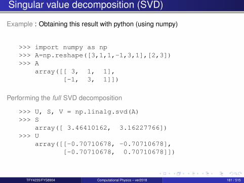
Singular value decomposition (SVD)
Example : Obtaining this result with python (using numpy)
>>> import numpy as np>>> A=np.reshape([3,1,1,-1,3,1],[2,3])>>> A
array([[ 3, 1, 1],[-1, 3, 1]])
Performing the full SVD decomposition
>>> U, S, V = np.linalg.svd(A)>>> S
array([ 3.46410162, 3.16227766])>>> U
array([[-0.70710678, -0.70710678],[-0.70710678, 0.70710678]])
TFY4235/FYS8904 Computational Physics – ver2018 181 / 515

Singular value decomposition (SVD)
Example : Using python to calculating the SVD decomposition of a matrix
Initialize numpy and a complex 9× 6 matrix
>>> import numpy as np>>> a = np.random.randn(9, 6) + 1j*np.random.randn(9, 6)
Reconstruction based on full SVD (convention used by python: a = USV
>>> U, s, V = np.linalg.svd(a, full_matrices=True)>>> U.shape, V.shape, s.shape((9, 9), (6, 6), (6,))>>> S = np.zeros((9, 6), dtype=complex)>>> S[:6, :6] = np.diag(s)>>> np.allclose(a, np.dot(U, np.dot(S, V))) # check a = U S VˆHTrue
Reconstruction based on reduced SVD
>>> U, s, V = np.linalg.svd(a, full_matrices=False)>>> U.shape, V.shape, s.shape((9, 6), (6, 6), (6,))>>> S = np.diag(s)>>> np.allclose(a, np.dot(U, np.dot(S, V)))True
TFY4235/FYS8904 Computational Physics – ver2018 182 / 515

Singular value decomposition (SVD)
Example : Using Fortran90 with LAPACK95 for SVD-calculation
program la_gesvd_example
use la_precision, only : wp = dpuse f95_lapack, only : la_gesvd
implicit nonereal(wp), allocatable :: S(:)complex(wp), allocatable :: A(:,:), U(:,:), VT(:,:)
.
.! Allocate storageallocate ( A(M,N), AA(M,N), U(M,M), VT(N,N), WW(1:MN-1) )
.
.write( *, * )’Details of LA_ZGESVD LAPACK Subroutine Results.’call la_gesvd( A, S, U, VT, WW, ’N’, INFO )
! NOTE : Vˆdagger is returned not V..
end program la_gesvd_example
SYNTAX:
LA_GESVD( A, S, [U=u], [VT=vt], [WW=ww], [JOB=job], [INFO=info] )
LAPACK95 : http://www.netlib.org/lapack95/lug95/
TFY4235/FYS8904 Computational Physics – ver2018 183 / 515

Singular value decomposition (SVD)
Syntax : Routine LA GESVD from LAPACK95 for SVD-calculations
SUBROUTINE LA_GESVD / LA_GESDD ( A, S, U=u, VT=vt, WW=ww, JOB=job, INFO=info )
type(wp), INTENT(INOUT) :: A(:,:)REAL(wp), INTENT(OUT) :: S(:)type(wp), INTENT(OUT), OPTIONAL :: U(:,:)type(wp), INTENT(OUT), OPTIONAL :: VT(:,:)REAL(wp), INTENT(OUT), OPTIONAL :: WW(:)CHARACTER(LEN=1), INTENT(IN), OPTIONAL :: JOBINTEGER, INTENT(OUT), OPTIONAL :: INFO
where
type ::= REAL / COMPLEX
wp ::= KIND(1.0) / KIND(1.0D0)
More information available from the LAPACK95 homepage :http://www.netlib.org/lapack95/lug95/
TFY4235/FYS8904 Computational Physics – ver2018 184 / 515
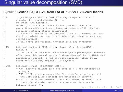
Singular value decomposition (SVD)
Syntax : Routine LA GESVD from LAPACK95 for SVD-calculations! A (input/output) REAL or COMPLEX array, shape (:, :) with! size(A, 1) = m and size(A, 2) = n.! On entry, the matrix A.! On exit, if JOB = ’U’ and U is not present, then A is! overwritten with the first min(m, n) columns of U (the left! singular vectors, stored columnwise).! If JOB = ’V’ and VT is not present, then A is overwritten with! the first min(m, n) rows of VˆH (the right singular vectors,! stored rowwise).! In all cases the original contents of A are destroyed.
! WW Optional (output) REAL array, shape (:) with size(WW) =! min(m, n) - 1! If INFO > 0, WW contains the unconverged superdiagonal elements! of an upper bidiagonal matrix B whose diagonal is in SIGMA (not! necessarily sorted). B has the same singular values as A.! Note: WW is a dummy argument for LA_GESDD.
! JOB Optional (input) CHARACTER(LEN=1).! = ’N’: neither columns of U nor rows of VˆH are returned in! array A.! = ’U’: if U is not present, the first min(m, n) columns of U! (the left singular vectors) are returned in array A;! = ’V’: if VT is not present, the first min(m, n) rows of VˆH! (the right singular vectors) are returned in array A;! Default value: ’N’.
TFY4235/FYS8904 Computational Physics – ver2018 185 / 515
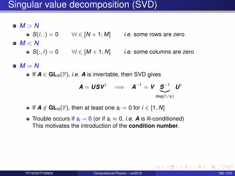
Singular value decomposition (SVD)
M > NS(i , :) = 0 ∀i ∈ [N + 1; M] i.e. some rows are zero
M < NS(:, i) = 0 ∀i ∈ [M + 1; N] i.e. some columns are zero
M = NIf A ∈ GLN(F), i.e. A is invertable, then SVD gives
A = USV † =⇒ A−1 = V S−1︸︷︷︸diag(1/si )
U†
If A /∈ GLN(F), then at least one si = 0 for i ∈ [1,N]
Trouble occurs if si = 0 (or if si ≈ 0, i.e. A is ill-conditioned)This motivates the introduction of the condition number.
TFY4235/FYS8904 Computational Physics – ver2018 186 / 515
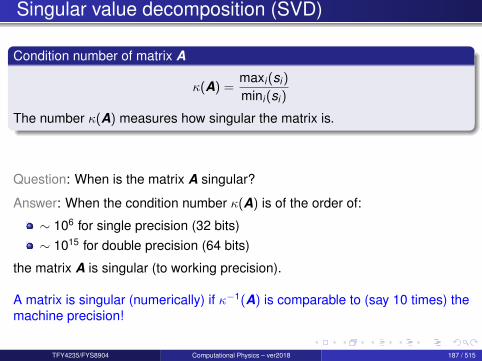
Singular value decomposition (SVD)
Condition number of matrix A
κ(A) =maxi (si )
mini (si )
The number κ(A) measures how singular the matrix is.
Question: When is the matrix A singular?
Answer: When the condition number κ(A) is of the order of:
∼ 106 for single precision (32 bits)∼ 1015 for double precision (64 bits)
the matrix A is singular (to working precision).
A matrix is singular (numerically) if κ−1(A) is comparable to (say 10 times) themachine precision!
TFY4235/FYS8904 Computational Physics – ver2018 187 / 515

Singular value decomposition (SVD)
What can we use the SVD decomposition for?
Application of the SVD decompositionOthonormal basis for range and null space of ACalculate the condition number of AMoore-Penrose pseudoinverseleast square calculations
TFY4235/FYS8904 Computational Physics – ver2018 188 / 515

Singular value decomposition (SVD)
Recall from Linear AlgebraThe range of A is the vector space R(A) = b : Ax = b (row space)The null space (or kernel) of A is the space N (A) = x : Ax = 0
The rank of A is the dimension of its range : rank (A) = dim(R(A))
The nullity of A is the dimension of its null space: nullity(A) = dim(N (A))
The rank-nullity theorem
Let A ∈ FM×N , then
rank(A) + nullity(A) = N
You will also see the notation:R(A) = range(A)
N (A) = null(A)
TFY4235/FYS8904 Computational Physics – ver2018 189 / 515

Singular value decomposition (SVD)
Orthogonal basisColumns of U corresponding to sii 6= 0 span R(A)Columns of V corresponding to sii ≈ 0 span N (A)
Non-Singular matrix : If A ∈ GLN(F) then:
R(R) = FN , rank(A) = NN (A) = 0FN , nullity(A) = 0
Singular matrix : If A is singular, Ax = b has no unique solution.However, one may ask for the vector x which minimizes the norm‖Ax − b‖. This vector x has the form
x =
nullity(A)∑i=1
cix(0)i + xp
where Ax (0)i = 0 and the “particular solution” xp — “best fit” (least
squares) solution to a system of linear equations — is obtained from theso-called pseudoinverse A+ (to be defined)
xp = A+b.TFY4235/FYS8904 Computational Physics – ver2018 190 / 515

Singular value decomposition (SVD)
The Moore-Penrose pseudoinverse
A pseudoinverse (or generalized inverse) A+ of a matrix A is a generalizationof the inverse matrix.
If A has the SVD decomposition
A = USV †
then its pseudoinverse A+ is obtained from
A+ = VS+U†
The pseudoinverse S+ of the diagonal matrix S is obtained by taking thereciprocal of each non-zero element on the diagonal, leaving the zeros inplace and taking the transpose of the result (if S is not a square matrix), i.e.
S =⇒ S+
sii 6= 0 =⇒ 1/sii
In Matlab and NumPy (numpy.linalg.pinv) the function pinv calculates A+!TFY4235/FYS8904 Computational Physics – ver2018 191 / 515
Singular value decomposition (SVD)
Least square solution
If Ax = b then
x = A+b
represents the least-squares approximate solutions that minimized the norm‖Ax − b‖.
This can be used to do linear regression by finding the linear least squaresolution.
TFY4235/FYS8904 Computational Physics – ver2018 192 / 515

Section 5
How to install libraries on a Linux system
TFY4235/FYS8904 Computational Physics – ver2018 193 / 515

Outline I
1 Introduction
2 Number representation and numerical precision
3 Finite differences and interpolation
4 Linear algebra
5 How to install libraries on a Linux system
6 Eigenvalue problems
7 Spectral methods
8 Numerical integration
TFY4235/FYS8904 Computational Physics – ver2018 194 / 515
Outline II9 Random numbers
10 Ordinary differential equations
11 Partial differential equations
12 Optimization
TFY4235/FYS8904 Computational Physics – ver2018 195 / 515
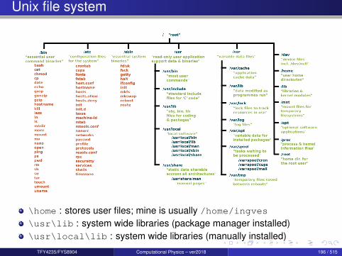
Unix file system
\home : stores user files; mine is usually /home/ingves\usr\lib : system wide libraries (package manager installed)\usr\local\lib : system wide libraries (manually installed)
TFY4235/FYS8904 Computational Physics – ver2018 196 / 515
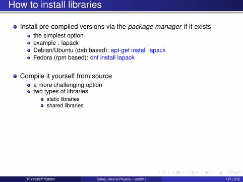
How to install libraries
Install pre-compiled versions via the package manager if it existsthe simplest optionexample : lapackDebian/Ubuntu (deb based): apt-get install lapackFedora (rpm based): dnf install lapack
Compile it yourself from sourcea more challenging optiontwo types of libraries
static librariesshared libraries
TFY4235/FYS8904 Computational Physics – ver2018 197 / 515

Different types of libraries
static librariesbinary code included in the executableExample gcc math library : libm.a
command : ar rvc “objectfiles”
shared librariesbinaray code not included the executablebinaray code takes from the shared library during executionthe shared library needs to be installed for program executionEx : libm.so
TFY4235/FYS8904 Computational Physics – ver2018 198 / 515

How to generate, make and use libraries (on Unix)
The main steps to generate a library are1 generate object files by compiling source files2 create the library
the method is different for static and shared libraries3 use the library when linking the object files
TFY4235/FYS8904 Computational Physics – ver2018 199 / 515
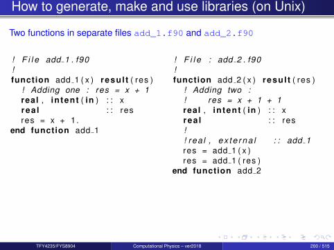
How to generate, make and use libraries (on Unix)
Two functions in separate files add_1.f90 and add_2.f90
! F i l e add 1 . f90!function add 1 ( x ) resul t ( res )
! Adding one : res = x + 1real , in tent ( in ) : : xrea l : : resres = x + 1.
end function add 1
! F i l e : add 2 . f90!function add 2 ( x ) resul t ( res )
! Adding two :! res = x + 1 + 1real , in tent ( in ) : : xrea l : : res!! rea l , ex te rna l : : add 1res = add 1 ( x )res = add 1 ( res )
end function add 2
TFY4235/FYS8904 Computational Physics – ver2018 200 / 515

How to generate, make and use libraries (on Unix)
The main program calling the function add_2()
program maini m p l i c i t nonerea l : : xreal , external : : add 2!x = 2.write (∗ ,∗ ) " x = " , xwrite (∗ ,∗ ) " x + 2 = " , add 2 ( x )!
end program main
TFY4235/FYS8904 Computational Physics – ver2018 201 / 515

How to generate, make and use libraries (on Unix)Compiling and running the program without the use of libraries
tux => l sadd 1 . f90 add 2 . f90 main . f90
tux => g f o r t r a n −o main add 2 . f90 add 1 . f90 main . f90
tux => l sadd 1 . f90 add 2 . f90 main main . f90
tux => . / mainx = 2.00000000x + 2 = 4.00000000
tux =>
TFY4235/FYS8904 Computational Physics – ver2018 202 / 515
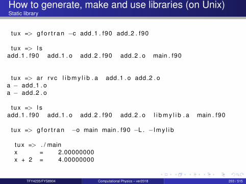
How to generate, make and use libraries (on Unix)Static library
tux => g f o r t r a n −c add 1 . f90 add 2 . f90
tux => l sadd 1 . f90 add 1 . o add 2 . f90 add 2 . o main . f90
tux => ar rvc l i b m y l i b . a add 1 . o add 2 . oa − add 1 . oa − add 2 . o
tux => l sadd 1 . f90 add 1 . o add 2 . f90 add 2 . o l i b m y l i b . a main . f90
tux => g f o r t r a n −o main main . f90 −L . − l m y l i b
tux => . / mainx = 2.00000000x + 2 = 4.00000000
TFY4235/FYS8904 Computational Physics – ver2018 203 / 515

How to generate, make and use libraries (on Unix)Shared library
1 make object files with Position Independent Code flag setgfortran -c -fPIC add_1.f90 add_2.f90
2 Creating a shared library from the object filegfortran -shared -o libMyLib.so add_1.o add_2.o
3 Linking with a shared librarygfortran -o Main main.f90 -L. -lMyLibHowever this requires that the compiler can find the shared librarylibMyLib.so
4 Making the library available at runtimeexport LD_LIBRARY_PATH=$LD_LIBRARY_PATH:.
TFY4235/FYS8904 Computational Physics – ver2018 204 / 515
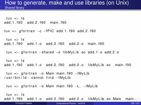
How to generate, make and use libraries (on Unix)Shared library
tux => l sadd 1 . f90 add 2 . f90 main . f90
tux => g f o r t r a n −c −fPIC add 1 . f90 add 2 . f90
tux => l sadd 1 . f90 add 1 . o add 2 . f90 add 2 . o main . f90
tux => g f o r t r a n −shared −o l ibMyL ib . so add 1 . o add 2 . o
tux => l sadd 1 . f90 add 1 . o add 2 . f90 add 2 . o l ibMyL ib . so main . f90
tux => g f o r t r a n −o Main main . f90 −lMyLib/ usr / b in / l d : cannot f i n d −lMyLib
tux => g f o r t r a n −o Main main . f90 −L . −lMyLib
tux => l sadd 1 . f90 add 1 . o add 2 . f90 add 2 . o l ibMyL ib . so Main main .
f90TFY4235/FYS8904 Computational Physics – ver2018 205 / 515

How to generate, make and use libraries (on Unix)Shared library
tux => . / Main. / Main : e r r o r while l oad ing shared l i b r a r i e s : l i bMyL ib . so :
cannot open shared ob jec t f i l e : No such f i l e or d i r e c t o r y
tux => l dd Mainl i nux−vdso . so .1 (0 x00007ffedd91b000 )l i bMyL ib . so => not foundl i b g f o r t r a n . so .3 => / usr / l i b / x86 64−l i nux−gnu /
l i b g f o r t r a n . so .3 (0 x00002af52c91f000 )l ibm . so .6 => / l i b / x86 64−l i nux−gnu / l ibm . so .6 (0
x00002af52cc45000 )l i b g c c s . so .1 => / l i b / x86 64−l i nux−gnu / l i b g c c s . so .1
(0 x00002af52cf49000 )l ibquadmath . so .0 => / usr / l i b / x86 64−l i nux−gnu /
l ibquadmath . so .0 (0 x00002af52d160000 )l i b c . so .6 => / l i b / x86 64−l i nux−gnu / l i b c . so .6 (0
x00002af52d3a1000 )/ l i b 6 4 / ld−l i nux−x86−64.so .2 (0 x000055d52b067000 )
tux => LD LIBRARY PATH=$LD LIBRARY PATH : . . / Mainx = 2.00000000x + 2 = 4.00000000
TFY4235/FYS8904 Computational Physics – ver2018 206 / 515
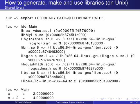
How to generate, make and use libraries (on Unix)Shared library
tux => export LD LIBRARY PATH=$LD LIBRARY PATH : .
tux => l dd Mainl i nux−vdso . so .1 (0 x00007f f f f4576000 )l i bMyL ib . so (0 x00002b8745f1c000 )l i b g f o r t r a n . so .3 => / usr / l i b / x86 64−l i nux−gnu /
l i b g f o r t r a n . so .3 (0 x00002b874613d000 )l ibm . so .6 => / l i b / x86 64−l i nux−gnu / l ibm . so .6 (0
x00002b8746463000 )l i b g c c s . so .1 => / l i b / x86 64−l i nux−gnu / l i b g c c s . so .1 (0
x00002b8746767000 )l ibquadmath . so .0 => / usr / l i b / x86 64−l i nux−gnu /
l ibquadmath . so .0 (0 x00002b874697e000 )l i b c . so .6 => / l i b / x86 64−l i nux−gnu / l i b c . so .6 (0
x00002b8746bbf000 )/ l i b 6 4 / ld−l i nux−x86−64.so .2 (0 x0000558b81992000 )
tux => Mainx = 2.00000000x + 2 = 4.00000000
TFY4235/FYS8904 Computational Physics – ver2018 207 / 515

How to generate, make and use libraries (on Unix)Compile your own library from source
Example : OpenBLAS — An optimized BLAS (and LAPACK) libraryurlwww.openblas.net/
1 Downloaded the latest version of the library from githubgit clone https://github.com/xianyi/OpenBLAS.git
2 Generation of serial library, domake USE_THREAD=0 FC=gfortran
3 Installed the library to ˜/Tmp/OpenBLAS (or whatever you prefer)make PREFIX=˜/Tmp/OpenBLAS/ install
4 (optional) OpenBLAS contains both the BLAS and LAPACK.However, most of my Makefiles have separate BLAS and LAPACK libraries.Therefore, for compatibility reasons, I prefer to make the following two linksin the installation directory
ln -s libopenblas.a libblas.aln -s libopenblas.a liblapack.a
For more details see https://pleiades.ucsc.edu/hyades/OpenBLAS
TFY4235/FYS8904 Computational Physics – ver2018 208 / 515

Section 6
Eigenvalue problems
TFY4235/FYS8904 Computational Physics – ver2018 209 / 515
Outline I
1 Introduction
2 Number representation and numerical precision
3 Finite differences and interpolation
4 Linear algebra
5 How to install libraries on a Linux system
6 Eigenvalue problems
7 Spectral methods
8 Numerical integration
TFY4235/FYS8904 Computational Physics – ver2018 210 / 515

Outline II9 Random numbers
10 Ordinary differential equations
11 Partial differential equations
12 Optimization
TFY4235/FYS8904 Computational Physics – ver2018 211 / 515
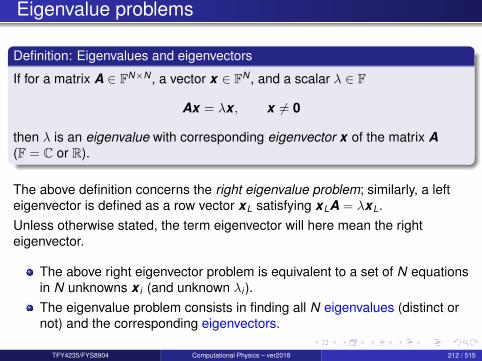
Eigenvalue problems
Definition: Eigenvalues and eigenvectors
If for a matrix A ∈ FN×N , a vector x ∈ FN , and a scalar λ ∈ F
Ax = λx , x 6= 0
then λ is an eigenvalue with corresponding eigenvector x of the matrix A(F = C or R).
The above definition concerns the right eigenvalue problem; similarly, a lefteigenvector is defined as a row vector xL satisfying xLA = λxL.Unless otherwise stated, the term eigenvector will here mean the righteigenvector.
The above right eigenvector problem is equivalent to a set of N equationsin N unknowns x i (and unknown λi ).The eigenvalue problem consists in finding all N eigenvalues (distinct ornot) and the corresponding eigenvectors.
TFY4235/FYS8904 Computational Physics – ver2018 212 / 515

Eigenvalue problems
The eigenvalue problem can be rewritten as
(A− λI) x = 0,
where I denotes the identity matrix.
This equation provides a solution to the problem if and only if the determinantis zero, namely
|A− λI | = 0,
which in turn means that the determinant is a polynomial of degree N in λ andin general we will have N distinct zeros.
TFY4235/FYS8904 Computational Physics – ver2018 213 / 515
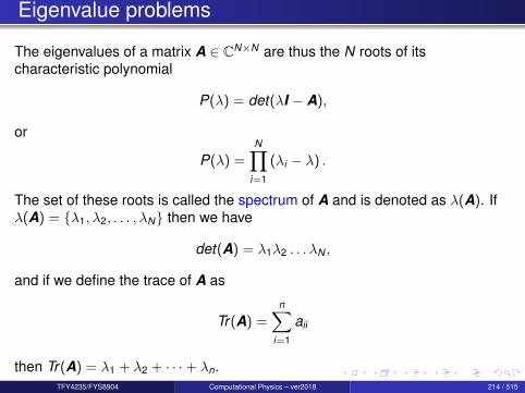
Eigenvalue problems
The eigenvalues of a matrix A ∈ CN×N are thus the N roots of itscharacteristic polynomial
P(λ) = det(λI − A),
or
P(λ) =N∏
i=1
(λi − λ) .
The set of these roots is called the spectrum of A and is denoted as λ(A). Ifλ(A) = λ1, λ2, . . . , λN then we have
det(A) = λ1λ2 . . . λN ,
and if we define the trace of A as
Tr(A) =n∑
i=1
aii
then Tr(A) = λ1 + λ2 + · · ·+ λn.TFY4235/FYS8904 Computational Physics – ver2018 214 / 515
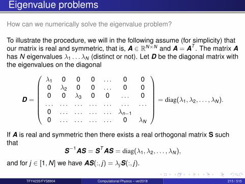
Eigenvalue problems
How can we numerically solve the eigenvalue problem?
To illustrate the procedure, we will in the following assume (for simplicity) thatour matrix is real and symmetric, that is, A ∈ RN×N and A = AT . The matrix Ahas N eigenvalues λ1 . . . λN (distinct or not). Let D be the diagonal matrix withthe eigenvalues on the diagonal
D =
λ1 0 0 0 . . . 0 00 λ2 0 0 . . . 0 00 0 λ3 0 0 . . . 0. . . . . . . . . . . . . . . . . . . . .0 . . . . . . . . . . . . λn−10 . . . . . . . . . . . . 0 λN
= diag(λ1, λ2, . . . , λN).
If A is real and symmetric then there exists a real orthogonal matrix S suchthat
S−1AS = ST AS = diag(λ1, λ2, . . . , λN),
and for j ∈ [1,N] we have AS(:, j) = λjS(:, j).
TFY4235/FYS8904 Computational Physics – ver2018 215 / 515
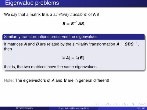
Eigenvalue problems
We say that a matrix B is a similarity transform of A if
B = S−1AS,
Similarity transformations preserves the eigenvalues
If matrices A and B are related by the similarity transformation A = SBS−1,then
λ(A) = λ(B),
that is, the two matrices have the same eigenvalues.
Note: The eigenvectors of A and B are in general different!
TFY4235/FYS8904 Computational Physics – ver2018 216 / 515
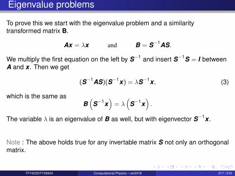
Eigenvalue problems
To prove this we start with the eigenvalue problem and a similaritytransformed matrix B.
Ax = λx and B = S−1AS.
We multiply the first equation on the left by S−1 and insert S−1S = I betweenA and x . Then we get
(S−1AS)(S−1x) = λS−1x , (3)
which is the same asB(
S−1x)
= λ(
S−1x).
The variable λ is an eigenvalue of B as well, but with eigenvector S−1x .
Note : The above holds true for any invertable matrix S not only an orthogonalmatrix.
TFY4235/FYS8904 Computational Physics – ver2018 217 / 515
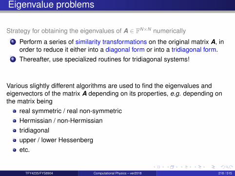
Eigenvalue problems
Strategy for obtaining the eigenvalues of A ∈ FN×N numerically1 Perform a series of similarity transformations on the original matrix A, in
order to reduce it either into a diagonal form or into a tridiagonal form.2 Thereafter, use specialized routines for tridiagonal systems!
Various slightly different algorithms are used to find the eigenvalues andeigenvectors of the matrix A depending on its properties, e.g. depending onthe matrix being
real symmetric / real non-symmetricHermissian / non-Hermissiantridiagonalupper / lower Hessenbergetc.
TFY4235/FYS8904 Computational Physics – ver2018 218 / 515
Eigenvalue problems
In short, the basic philosophy of finding eigenvalues/eigenvectors are:
either apply subsequent similarity transformations (direct method) so that
STN . . .S
T1 A S1 . . .SN = D,
or apply subsequent similarity transformations so that A becomestridiagonal (Householder) or upper/lower triangular (QR method).Thereafter, techniques for obtaining eigenvalues from tridiagonalmatrices can be used.
or use so-called power methods
or use iterative methods (Krylov, Lanczos, Arnoldi).These methods are popular for huge matrix problems.
TFY4235/FYS8904 Computational Physics – ver2018 219 / 515

Eigenvalue problems
General recommendation for numerically solving eigenvalue problems
Dense matrices of order “N ≤ 105”use library routines (LAPACK)Computational complexity: O(N3) when A ∈ FN×N
Sparse matrices/dense (“N ≥ 105”)use iterative techniques (ARPACK and TRLAN; FORTRAN libraries)
LanczosArnoldiKrylov
The field of solving eigensystems is a complex matter, so we will not cover therather technical details here!
TFY4235/FYS8904 Computational Physics – ver2018 220 / 515
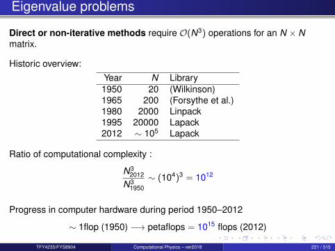
Eigenvalue problems
Direct or non-iterative methods require O(N3) operations for an N × Nmatrix.
Historic overview:Year N Library1950 20 (Wilkinson)1965 200 (Forsythe et al.)1980 2000 Linpack1995 20000 Lapack2012 ∼ 105 Lapack
Ratio of computational complexity :
N32012
N31950
∼ (104)3 = 1012
Progress in computer hardware during period 1950–2012
∼ 1flop (1950) −→ petaflops = 1015 flops (2012)
TFY4235/FYS8904 Computational Physics – ver2018 221 / 515
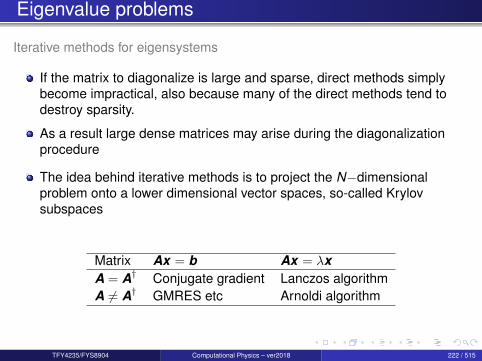
Eigenvalue problems
Iterative methods for eigensystems
If the matrix to diagonalize is large and sparse, direct methods simplybecome impractical, also because many of the direct methods tend todestroy sparsity.
As a result large dense matrices may arise during the diagonalizationprocedure
The idea behind iterative methods is to project the N−dimensionalproblem onto a lower dimensional vector spaces, so-called Krylovsubspaces
Matrix Ax = b Ax = λxA = A† Conjugate gradient Lanczos algorithmA 6= A† GMRES etc Arnoldi algorithm
TFY4235/FYS8904 Computational Physics – ver2018 222 / 515
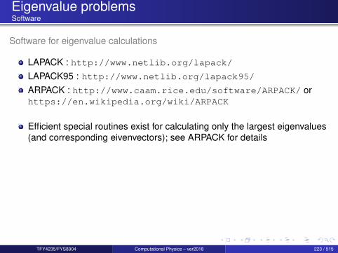
Eigenvalue problemsSoftware
Software for eigenvalue calculations
LAPACK : http://www.netlib.org/lapack/LAPACK95 : http://www.netlib.org/lapack95/ARPACK : http://www.caam.rice.edu/software/ARPACK/ orhttps://en.wikipedia.org/wiki/ARPACK
Efficient special routines exist for calculating only the largest eigenvalues(and corresponding eivenvectors); see ARPACK for details
TFY4235/FYS8904 Computational Physics – ver2018 223 / 515

Eigenvalue problems
Generalized Eigenssystems
Let A and B be matrices of the compatible dimensions.
Then following system is referred to as the generalized eigensystem
Ax = λBx
Technically it is equivalent to solving B−1Ax = λx , but B−1 is computationallyexpensive to obtain.
These problems are solved by LAPACK in an efficient way (without firstcalculating B−1)!
TFY4235/FYS8904 Computational Physics – ver2018 224 / 515

The remaining slides of this section were not covered in the lectures
TFY4235/FYS8904 Computational Physics – ver2018 225 / 515

Largest eigenvalue (not covered in the lectures)
If only one eigenvalue is to be determined — or just a few — includingcorresponding eigenvectors, one may use simple iterative methods.We assume Sp(A) ⊂ R for simplicity. Let λm = max(Sp(A)).
Iteration scheme
X ′k = AXk−1
Xk =X ′k‖X ′k‖
We will denote Vi a normalized eigenvector associated to the eigenvalueλi .
TFY4235/FYS8904 Computational Physics – ver2018 226 / 515
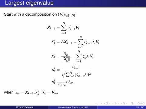
Largest eigenvalue
Start with a decomposition on (Vi )i∈J1;NK:
Xk−1 =N∑
i=1
c ik−1Vi
X ′k = AXk−1 =N∑
i=1
c ik−1λiVi
Xk =X ′k‖X ′k‖
=N∑
i=1
c ikλiVi
c ik =
c ik−1√∑N
i=1(c ik−1λi )2
c ik −−−→k→∞
δim
when λm = Xk−1.X ′k , Xk = Vm.
TFY4235/FYS8904 Computational Physics – ver2018 227 / 515

Determining any eigenvalue
We still assume Sp(A) ⊂ R.
(A− λIN)−1Vj =1
λj − λVj
Iteration scheme
X ′k = (A− λIN)−1Xk−1
Xk =X ′k‖X ′k‖
Converges to the eigenvalue closest to λ
λj = λ+1
Xk−1.X ′k
TFY4235/FYS8904 Computational Physics – ver2018 228 / 515
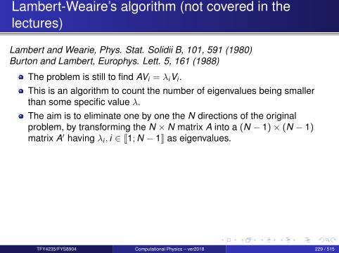
Lambert-Weaire’s algorithm (not covered in thelectures)
Lambert and Wearie, Phys. Stat. Solidii B, 101, 591 (1980)Burton and Lambert, Europhys. Lett. 5, 161 (1988)
The problem is still to find AVi = λiVi .This is an algorithm to count the number of eigenvalues being smallerthan some specific value λ.The aim is to eliminate one by one the N directions of the originalproblem, by transforming the N × N matrix A into a (N − 1)× (N − 1)matrix A′ having λi , i ∈ J1; N − 1K as eigenvalues.
TFY4235/FYS8904 Computational Physics – ver2018 229 / 515
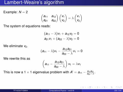
Lambert-Weaire’s algorithm
Example: N = 2 (a11 a12a21 a22
)(v1v2
)= λ
(v1v2
)The system of equations reads:
(a11 − λ)v1 + a12v2 = 0a21v1 + (a22 − λ)v2 = 0
We eliminate v2.(a11 − λ)v1 −
a12a21
a22 − λv1 = 0
We rewrite this as (a11 −
a12a21
a22 − λ
)v1 = λv1
This is now a 1× 1 eigenvalue problem with A′ = a11 − a12a21a22−λ .
TFY4235/FYS8904 Computational Physics – ver2018 230 / 515

Lambert-Weaire’s algorithm
The N × N case. ∀i ∈ J1,NK,
N∑j=1
aijvj = λvi
We eliminate vN and findN−1∑j=1
a′ijvj = λvi
where a′ij = aij − aiN aNjaNN−λ . We do this recursively:
(*)
a(k)ij = a(k−1)
ij −a(k−1)
i,N−k+1a(k−1)N−k+1,j
a(k−1)N−k+1,N−k+1 − λ
TFY4235/FYS8904 Computational Physics – ver2018 231 / 515

Lambert-Weaire’s algorithm
If we now choose a value λ, the negative eigenvalue theorem states that thenumber of eigenvalues verifying λi < λ is equal to the number of times thedenominator in (*) - (a(k−1)
N−k+1,N−k+1 − λ) - has been negative for k = 1, · · · ,N.This is a simple, powerful, and largely forgotten algorithm!
TFY4235/FYS8904 Computational Physics – ver2018 232 / 515

Section 7
Spectral methods
TFY4235/FYS8904 Computational Physics – ver2018 233 / 515

Outline I
1 Introduction
2 Number representation and numerical precision
3 Finite differences and interpolation
4 Linear algebra
5 How to install libraries on a Linux system
6 Eigenvalue problems
7 Spectral methodsFourier transformWavelet transform
TFY4235/FYS8904 Computational Physics – ver2018 234 / 515
Outline II8 Numerical integration
9 Random numbers
10 Ordinary differential equations
11 Partial differential equations
12 Optimization
TFY4235/FYS8904 Computational Physics – ver2018 235 / 515
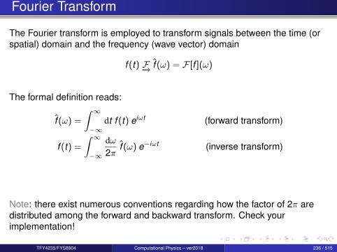
Fourier Transform
The Fourier transform is employed to transform signals between the time (orspatial) domain and the frequency (wave vector) domain
f (t) F−→ f (ω) = F [f ](ω)
The formal definition reads:
f (ω) =
∫ ∞−∞
dt f (t) eiωt (forward transform)
f (t) =
∫ ∞−∞
dω2π
f (ω) e−iωt (inverse transform)
Note: there exist numerous conventions regarding how the factor of 2π aredistributed among the forward and backward transform. Check yourimplementation!
TFY4235/FYS8904 Computational Physics – ver2018 236 / 515
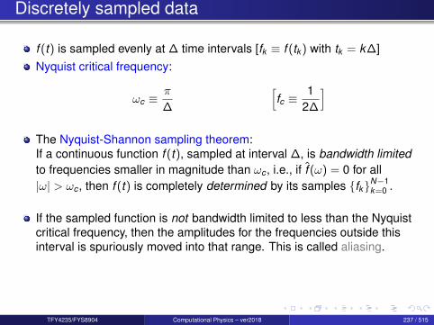
Discretely sampled data
f (t) is sampled evenly at ∆ time intervals [fk ≡ f (tk ) with tk = k∆]Nyquist critical frequency:
ωc ≡π
∆
[fc ≡
12∆
]The Nyquist-Shannon sampling theorem:If a continuous function f (t), sampled at interval ∆, is bandwidth limitedto frequencies smaller in magnitude than ωc , i.e., if f (ω) = 0 for all|ω| > ωc , then f (t) is completely determined by its samples fkN−1
k=0 .
If the sampled function is not bandwidth limited to less than the Nyquistcritical frequency, then the amplitudes for the frequencies outside thisinterval is spuriously moved into that range. This is called aliasing.
TFY4235/FYS8904 Computational Physics – ver2018 237 / 515
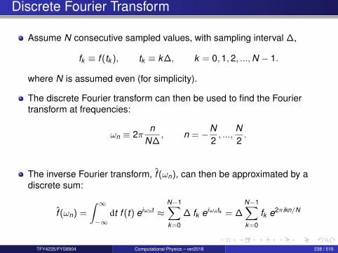
Discrete Fourier Transform
Assume N consecutive sampled values, with sampling interval ∆,
fk ≡ f (tk ), tk ≡ k∆, k = 0,1,2, ...,N − 1.
where N is assumed even (for simplicity).
The discrete Fourier transform can then be used to find the Fouriertransform at frequencies:
ωn ≡ 2πn
N∆, n = −N
2, ...,
N2.
The inverse Fourier transform, f (ωn), can then be approximated by adiscrete sum:
f (ωn) =
∫ ∞−∞
dt f (t) eiωnt ≈N−1∑k=0
∆ fk eiωntk = ∆N−1∑k=0
fk e2πikn/N
TFY4235/FYS8904 Computational Physics – ver2018 238 / 515
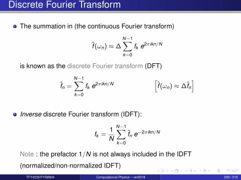
Discrete Fourier Transform
The summation in (the continuous Fourier transform)
f (ωn) ≈ ∆N−1∑k=0
fk e2πikn/N
is known as the discrete Fourier transform (DFT)
fn =N−1∑k=0
fk e2πikn/N[f (ωn) ≈ ∆fn
]
Inverse discrete Fourier transform (IDFT):
fk =1N
N−1∑k=0
fn e−2πikn/N
Note : the prefactor 1/N is not always included in the IDFT
(normalized/non-normalized IDFT)
TFY4235/FYS8904 Computational Physics – ver2018 239 / 515

Discrete Fourier Transform
How much computation is involved in doing the discrete Fourier transform?
WN ≡ e2πi/N =⇒ fn =N−1∑k=0
W nkN fk
The vector of fk ’s is multiplied by a matrix with (n,k)th element equal WNto the power nk , resulting in the vector of fn’s. This matrix multiplication,and therefore the discrete Fourier transform, is an O(N2) process.
Using an algorithm called the fast Fourier transform (FFT), it is possibleto compute the discrete Fourier transform in O(N log2 N) operations.
TFY4235/FYS8904 Computational Physics – ver2018 240 / 515

Fast Fourier Transform (FFT)
The basic idea behind the (radix-2) FFT8 is to write the Fourier transform overN points as two Fourier transforms over N/2 points.9
One way this can be derived is through the Danielson-Lanczos lemma:
fn =N−1∑k=0
fk W nkN , WN = e2πi/N (N’th root of unity)
=
N/2−1∑k=0
f2k W n(2k)N +
N/2−1∑k=0
f2k+1 W n(2k+1)N
=
N/2−1∑k=0
f2k W nkN/2 + W n
N
N/2−1∑k=0
f2k+1 W nkN/2
= f en + W n
N f on
8For more info see Wikipedia.9The FFT-method was popularized by a publication of J. W. Cooley and J. W. Tukey in 1965,
but it was later (1984) discovered that those two authors had independently re-invented analgorithm known to Carl Friedrich Gauss around 1805.
TFY4235/FYS8904 Computational Physics – ver2018 241 / 515
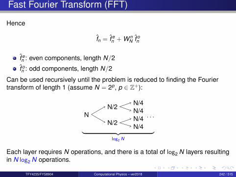
Fast Fourier Transform (FFT)
Hence
fn = f en + W n
N f on
f en : even components, length N/2
f on : odd components, length N/2
Can be used recursively until the problem is reduced to finding the Fouriertransform of length 1 (assume N = 2p, p ∈ Z+):
NN/2 N/4
N/4
N/2 N/4N/4
· · ·
︸ ︷︷ ︸log2 N
Each layer requires N operations, and there is a total of log2 N layers resultingin N log2 N operations.
TFY4235/FYS8904 Computational Physics – ver2018 242 / 515
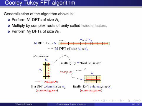
Cooley-Tukey FFT algorithm
Generalization of the algorithm above is:Perform N1 DFTs of size N2.Multiply by complex roots of unity called twiddle factors.Perform N2 DFTs of size N1.
TFY4235/FYS8904 Computational Physics – ver2018 243 / 515

Examples FFT
numpy: real-to-complex>>> impor t numpy as np>>> x=np . random . rand ( 8 )>>> xar ray ( [ 0.54528432 , 0.53861951 , 0.44141222 , 0.30055361 ,
0.66794224 , 0.53216542 , 0.78834189 , 0.77609837])
>>> X=np . f f t . r f f t ( x )>>> Xar ray ( [ 4.59041758+0. j , 0.21816672+0.67862686 j ,
−0.01652755+0.00586704 j , −0.46348258−0.01523247 j ,0.29554377+0. j ] )
>>> np . f f t . i r f f t (X)ar ray ( [ 0.54528432 , 0.53861951 , 0.44141222 , 0.30055361 ,
0.66794224 , 0.53216542 , 0.78834189 , 0.77609837])
>>> x .sum ( )4.5904175817116109
The transform np.fft.rfft(x) is normalized!TFY4235/FYS8904 Computational Physics – ver2018 244 / 515
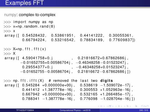
Examples FFT
numpy: complex-to-complex
>>> impor t numpy as np>>> x=np . random . rand ( 8 )>>> xar ray ( [ 0.54528432 , 0.53861951 , 0.44141222 , 0.30055361 ,
0.66794224 , 0.53216542 , 0.78834189 , 0.77609837])
>>> X=np . f f t . f f t ( x )>>> Xar ray ( [ 4.59041758+0. j , 0.21816672+0.67862686 j ,
−0.01652755+0.00586704 j , −0.46348258−0.01523247 j ,0.29554377+0. j , −0.46348258+0.01523247 j ,−0.01652755−0.00586704 j , 0.21816672−0.67862686 j ] )
>>> np . f f t . i f f t (X) # removed the l a s t two dig i tsar ray ( [ 0.545284 +0.000000e+00 j , 0.538619 −1.509072e−17j ,
0.441412 +1.387778e−16j , 0.300553 +1.052963e−16j ,0.667942 +0.000000e+00 j , 0.532165 +1.266485e−17j ,0.788341 −1.387778e−16j , 0.776098 −1.028704e−16 j ] )
TFY4235/FYS8904 Computational Physics – ver2018 245 / 515
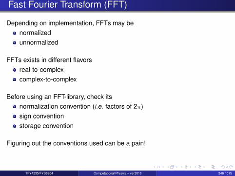
Fast Fourier Transform (FFT)
Depending on implementation, FFTs may benormalizedunnormalized
FFTs exists in different flavorsreal-to-complexcomplex-to-complex
Before using an FFT-library, check itsnormalization convention (i.e. factors of 2π)sign conventionstorage convention
Figuring out the conventions used can be a pain!
TFY4235/FYS8904 Computational Physics – ver2018 246 / 515

FFT Software
Use a library for doing FFTs!
Software for doing FFTs:FFTW : Fastest Fourier Transform in the west — www.fftw.org/
FFTPACK : www.netlib.org/fftpack/
GSL: GNU scientific Library — www.gnu.org/software/gsl/
SLATEC : www.netlib.org/slatec/
scipy : www.netlib.org/slatec/
TFY4235/FYS8904 Computational Physics – ver2018 247 / 515

Why are Fourier transforms so useful?
Physical description is sometimes simpler in the Fourier domain (FD)
Some mathematical operations are simpler in the FD (e.g. ODEs)
Periodic signals are often of interest.
Harmonic dependence/Superposition
Some numerical operations can be done much faster via FFTs (e.g.convolutions)
TFY4235/FYS8904 Computational Physics – ver2018 248 / 515
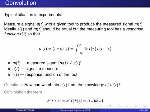
Convolution
Typical situation in experiments:
Measure a signal s(t) with a given tool to produce the measured signal m(t).Ideally s(t) and m(t) should be equal but the measuring tool has a responsefunction r(t) so that
m(t) = (r ∗ s) (t) =
∫ ∞−∞
dτ r(τ) s(t − τ)
m(t) — measured signal [m(t) 6= s(t)]s(t) — signal to measurer(t) — response function of the tool
Question : How can we obtain s(t) from the knowledge of m(t)?
Convolution theorem
F [r ∗ s] = F [r ]F [s] = r(ω)s(ω)
TFY4235/FYS8904 Computational Physics – ver2018 249 / 515

Convolution
The convolution operation
(r ∗ s)(t) =
∫ ∞−∞
dτ r(τ) s(t − τ)
can be discretized and defined like:
s(t)→ sj , r(t)→ rj ,
(r ∗ s)j ≡M/2∑
k=−M/2+1
rk sj−k .
Here M is the finite duration of the response function.
rk 6= 0 for −M/2 ≤ k ≤ M/2.
TFY4235/FYS8904 Computational Physics – ver2018 250 / 515
Convolution - Interpretation of rj
Input signal sj in channel j :r0 gives how much of sj remains in channel j .r1 gives how much of sj is sent into channel j + 1.And so on. . .
Identity response:r0 = 1, rk = 0, k 6= 0
TFY4235/FYS8904 Computational Physics – ver2018 251 / 515

Convolution - Interpretation of rj
(f ∗ g)(t) =
∫ ∞−∞
dτ f (τ) g(t − τ)
TFY4235/FYS8904 Computational Physics – ver2018 252 / 515
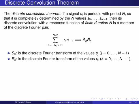
Discrete Convolution Theorem
The discrete convolution theorem: If a signal sj is periodic with period N, sothat it is completeley determined by the N values s0, . . . , sN−1, then itsdiscrete convolution with a response function of finite duration N is a memberof the discrete Fourier pair,
N/2∑k=−N/2+1
rk sj−k ⇐⇒ SnRn
Sn: is the discrete Fourier transform of the values sj (j = 0, . . . ,N − 1)Rn: is the discrete Fourier transform of the values rk (k = 0, . . . ,N − 1)
TFY4235/FYS8904 Computational Physics – ver2018 253 / 515
Treatment of end effects by zero padding
Almost always, one is interested in a response function whose duration Mis much shorter than the length of the data set N. In this case one cansimply extend the response function to length N by padding it with zeros.
If s is not periodic with period N, then data from “higher” channels will befolded into the 0 channel. This can be fixed by adding zero padding:
sk = 0, k = N + 1, . . . ,N + M.
TFY4235/FYS8904 Computational Physics – ver2018 254 / 515
Deconvolution
To try and undo the smearing done to a dataset from a known responsefunction, the function
(r ∗ s)j︸ ︷︷ ︸known
≡N/2∑
k=−N/2+1
rk︸︷︷︸known
sj−k︸︷︷︸unknown
is solved with respect to sj . This is a set of simultaneous linear equations thatis unrealistic to solve in most cases.
The problem can be solved very quickly using the FFT. Just divide thetransform of the convolution by the transform of the response to get thetransform of the deconvoluted signal.
This procedure won’t work if Rn = 0. This indicated that the originalconvolution has lost all information at that one frequency. The process isalso generally sensitive to noise in the input and to how well the responserk is known.
TFY4235/FYS8904 Computational Physics – ver2018 255 / 515

Wavelet transform
To be written!
TFY4235/FYS8904 Computational Physics – ver2018 256 / 515

Section 8
Numerical integration
TFY4235/FYS8904 Computational Physics – ver2018 257 / 515

Outline I
1 Introduction
2 Number representation and numerical precision
3 Finite differences and interpolation
4 Linear algebra
5 How to install libraries on a Linux system
6 Eigenvalue problems
7 Spectral methods
8 Numerical integrationOne-dimensional integration
TFY4235/FYS8904 Computational Physics – ver2018 258 / 515

Outline IIMultidimensional integrals
9 Random numbers
10 Ordinary differential equations
11 Partial differential equations
12 Optimization
TFY4235/FYS8904 Computational Physics – ver2018 259 / 515
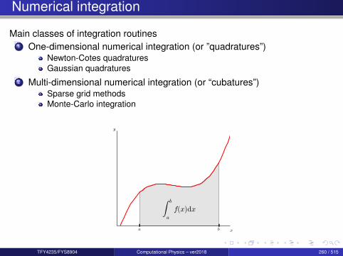
Numerical integration
Main classes of integration routines1 One-dimensional numerical integration (or ”quadratures”)
Newton-Cotes quadraturesGaussian quadratures
2 Multi-dimensional numerical integration (or “cubatures”)Sparse grid methodsMonte-Carlo integration
a b
∫ b
a
f(x)dx
x
y
TFY4235/FYS8904 Computational Physics – ver2018 260 / 515
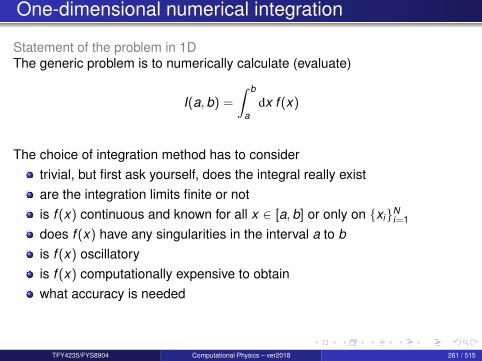
One-dimensional numerical integration
Statement of the problem in 1DThe generic problem is to numerically calculate (evaluate)
I(a,b) =
∫ b
adx f (x)
The choice of integration method has to considertrivial, but first ask yourself, does the integral really existare the integration limits finite or notis f (x) continuous and known for all x ∈ [a,b] or only on xiN
i=1
does f (x) have any singularities in the interval a to bis f (x) oscillatoryis f (x) computationally expensive to obtainwhat accuracy is needed
TFY4235/FYS8904 Computational Physics – ver2018 261 / 515
One-dimensional numerical integration
A change of variable may be useful!
Definite integrals∫ b
adx f (x) =
b − a2
∫ 1
−1du f
(b − a
2u +
b + a2
); x =
b − a2
u +b + a
2
Improper integrals∫ ∞0
dx f (x) =
∫ 1
0du
f( 1
u − 1)
u2 ; x =1u− 1
∫ ∞−∞
dx f (x) =
∫ ∞0
dx [f (x) + f (−x)]
or use the transformation x = (1− u)/u (which maps the entire real line on[0,1]).
TFY4235/FYS8904 Computational Physics – ver2018 262 / 515
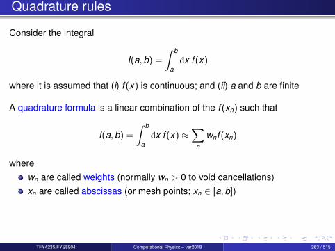
Quadrature rules
Consider the integral
I(a,b) =
∫ b
adx f (x)
where it is assumed that (i) f (x) is continuous; and (ii) a and b are finite
A quadrature formula is a linear combination of the f (xn) such that
I(a,b) =
∫ b
adx f (x) ≈
∑n
wnf (xn)
wherewn are called weights (normally wn > 0 to void cancellations)xn are called abscissas (or mesh points; xn ∈ [a,b])
TFY4235/FYS8904 Computational Physics – ver2018 263 / 515

Quadrature rules
Two main classes:
Newton-Cotes quadraturesthe abscissas xn are equally spaced, and the weights wn are determinedso that the formula is exact for polynomials of as high degree as possible.
xn given and wn determined
Gaussian quadratureboth the abscissas xn and the weights wn are chosen so that the formulais exact for polynomials of as high a degree as possible.This leads to non-equidistant xn’s!
both xn and wn are determined
TFY4235/FYS8904 Computational Physics – ver2018 264 / 515

Quadrature rules
CommentsIf the function f (x) is given explicitly instead of simply being tabulated atthe values xn, the best numerical method is the Gaussian quadratures
By picking the abscissas xn to sample the function, the Gaussianquadrature produces more accurate approximations for the same numberof points
However, the Gaussian quadratures are significantly more complicated toimplement than the Newton-Cotes quadratures.
TFY4235/FYS8904 Computational Physics – ver2018 265 / 515
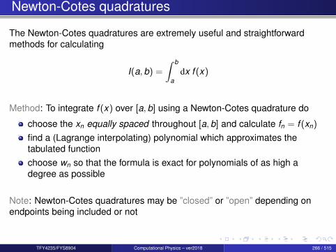
Newton-Cotes quadratures
The Newton-Cotes quadratures are extremely useful and straightforwardmethods for calculating
I(a,b) =
∫ b
adx f (x)
Method: To integrate f (x) over [a,b] using a Newton-Cotes quadrature do
choose the xn equally spaced throughout [a,b] and calculate fn = f (xn)
find a (Lagrange interpolating) polynomial which approximates thetabulated functionchoose wn so that the formula is exact for polynomials of as high adegree as possible
Note: Newton-Cotes quadratures may be ”closed” or ”open” depending onendpoints being included or not
TFY4235/FYS8904 Computational Physics – ver2018 266 / 515
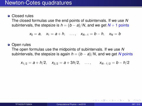
Newton-Cotes quadratures
Closed rulesThe closed formulas use the end points of subintervals. If we use Nsubintervals, the stepsize is h = (b − a)/N, and we get N + 1 points
x0 = a, x1 = a + h, . . . , xN−1 = b − h, xN = b
Open rulesThe open formulas use the midpoints of subintervals. If we use Nsubintervals, the stepsize is again h = (b − a)/N, and we get N points
x1/2 = a + h/2, x3/2 = a + 3h/2, . . . , xN−1/2 = b − h/2
TFY4235/FYS8904 Computational Physics – ver2018 267 / 515
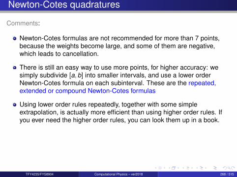
Newton-Cotes quadratures
Comments:
Newton-Cotes formulas are not recommended for more than 7 points,because the weights become large, and some of them are negative,which leads to cancellation.
There is still an easy way to use more points, for higher accuracy: wesimply subdivide [a,b] into smaller intervals, and use a lower orderNewton-Cotes formula on each subinterval. These are the repeated,extended or compound Newton-Cotes formulas
Using lower order rules repeatedly, together with some simpleextrapolation, is actually more efficient than using higher order rules. Ifyou ever need the higher order rules, you can look them up in a book.
TFY4235/FYS8904 Computational Physics – ver2018 268 / 515

Newton-Cotes quadratures
Some Classical Newton-Cotes quadratures
Midpoint rule: open 1 point Newton-Cotes quadrature (N = 1)Trapezoidal rule: closed 2 point Newton-Cotes quadrature (N = 1)Simpson’s rule: closed 3 point Newton-Cotes quadrature (N = 2)
We will now revisit these methods!
TFY4235/FYS8904 Computational Physics – ver2018 269 / 515

Midpoint rule (or Rectangle method)
Local rule: With only one point, we can onlyinterpolate a polynomial of degree 0, i.e. aconstant.∫ b
af (x) dx ≈ (b − a) f
(a + b
2
)Local error : (b−a)3
24 f (2)(ξ), ξ ∈ [a,b]
Extended formula (open); Repeated midpoint rule (x0 = a; xN = b)∫ b
af (x) dx =
∫ x1
x0
f (x) dx +
∫ x2
x1
f (x) dx + . . .
∫ xN
xN−1
f (x) dx ; h =b − a
N
≈ h[f (x1/2) + f (x3/2) + . . .+ f (xN−1/2)
]= h
N∑n=1
f (xn−1/2),
Global error : (b−a)h2
24 f (2)(ξ) = O(h2)
TFY4235/FYS8904 Computational Physics – ver2018 270 / 515

Trapezoidal rule
Local rule: We have two points, so we caninterpolate a polynomial of degree 1, i.e. astraight line.∫ b
af (x) dx ≈b − a
2[f (a) + f (b)]
Local error : − (b−a)3
12 f (2)(ξ), ξ ∈ [a,b]
Extended formula (closed)
∫ b
af (x) dx ≈ h
[12
f (x0) + f (x1) + f (x2) + . . .+ f (xN−1) +12
f (xN)
],
xn = x0 + nh
Global error : − (b−a)h2
12 f (2)(ξ) = O(h2)
TFY4235/FYS8904 Computational Physics – ver2018 271 / 515
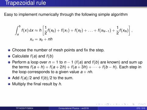
Trapezoidal rule
Easy to implement numerically through the following simple algorithm
∫ b
af (x) dx ≈ h
[12
f (x0) + f (x1) + f (x2) + . . .+ f (xN−1) +12
f (xN)
],
xn = x0 + nh
Choose the number of mesh points and fix the step.Calculate f (a) and f (b)
Perform a loop over n = 1 to n − 1 (f (a) and f (b) are known) and sum upthe terms f (a + h) + f (a + 2h) + f (a + 3h) + · · ·+ f (b − h). Each step inthe loop corresponds to a given value a + nh.Add f (a)/2 and f (b)/2 to the sum.Multiply the final result by h.
TFY4235/FYS8904 Computational Physics – ver2018 272 / 515
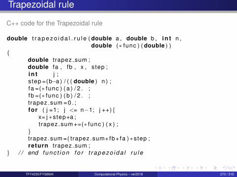
Trapezoidal rule
C++ code for the Trapezoidal rule
double t r a p e z o i d a l r u l e ( double a , double b , i n t n ,double (∗ func ) ( double ) )
double trapez sum ;double fa , fb , x , step ;i n t j ;s tep =(b−a ) / ( ( double ) n ) ;fa =(∗ func ) ( a ) / 2 . ;fb =(∗ func ) ( b ) / 2 . ;trapez sum = 0 . ;for ( j =1; j <= n−1; j ++)
x= j ∗step+a ;trapez sum +=(∗ func ) ( x ) ;
trapez sum =( trapez sum+fb+ fa ) ∗step ;return trapez sum ;
/ / end f u n c t i o n f o r t r a p e z o i d a l r u l e
TFY4235/FYS8904 Computational Physics – ver2018 273 / 515

Trapezoidal rule
Pay attention to the way we transfer the name of a function. This gives us thepossibility to define a general trapezoidal method, where we give as input thename of the function.
double t r a p e z o i d a l r u l e ( double a , double b , i n t n ,double (∗ func ) ( double ) )
We call this function simply as something like this
i n t e g r a l = t r a p e z o i d a l r u l e ( a , b , n , mysuperduperfunct ion ) ;
TFY4235/FYS8904 Computational Physics – ver2018 274 / 515
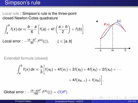
Simpson’s rule
Local rule : Simpson’s rule is the three-pointclosed Newton-Cotes quadrature∫ b
af (x) dx ≈ b − a
6
[f (a) + 4f
(a + b
2
)+ f (b)
].
Local error : − (b−a)5
90 f (4)(ξ), ξ ∈ [a,b]
Extended formula (closed)∫ b
af (x) dx ≈ h
3
[f (x0) + 4f (x1) + 2f (x2) + 4f (x3) + 2f (x4) + · · ·
+ 4f (xN−1) + f (xN)
].
Global error : − (b−a)h4
180 f (4)(ξ) = O(h4)
TFY4235/FYS8904 Computational Physics – ver2018 275 / 515
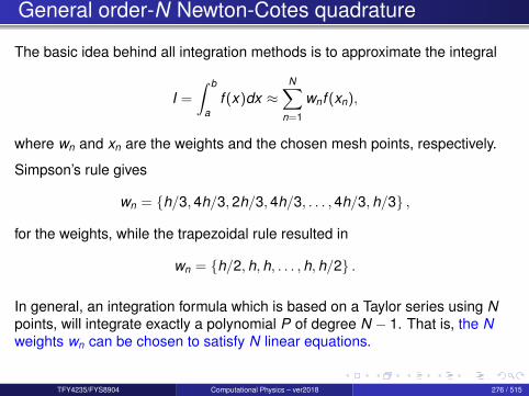
General order-N Newton-Cotes quadrature
The basic idea behind all integration methods is to approximate the integral
I =
∫ b
af (x)dx ≈
N∑n=1
wnf (xn),
where wn and xn are the weights and the chosen mesh points, respectively.
Simpson’s rule gives
wn = h/3,4h/3,2h/3,4h/3, . . . ,4h/3,h/3 ,
for the weights, while the trapezoidal rule resulted in
wn = h/2,h,h, . . . ,h,h/2 .
In general, an integration formula which is based on a Taylor series using Npoints, will integrate exactly a polynomial P of degree N − 1. That is, the Nweights wn can be chosen to satisfy N linear equations.
TFY4235/FYS8904 Computational Physics – ver2018 276 / 515
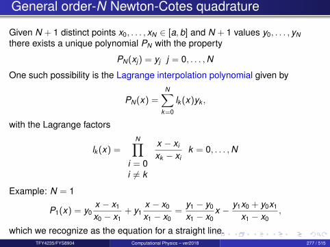
General order-N Newton-Cotes quadrature
Given N + 1 distinct points x0, . . . , xN ∈ [a,b] and N + 1 values y0, . . . , yNthere exists a unique polynomial PN with the property
PN(xj ) = yj j = 0, . . . ,N
One such possibility is the Lagrange interpolation polynomial given by
PN(x) =N∑
k=0
lk (x)yk ,
with the Lagrange factors
lk (x) =N∏
i = 0i 6= k
x − xi
xk − xik = 0, . . . ,N
Example: N = 1
P1(x) = y0x − x1
x0 − x1+ y1
x − x0
x1 − x0=
y1 − y0
x1 − x0x − y1x0 + y0x1
x1 − x0,
which we recognize as the equation for a straight line.TFY4235/FYS8904 Computational Physics – ver2018 277 / 515
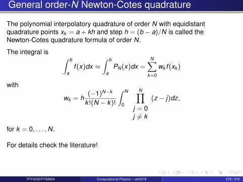
General order-N Newton-Cotes quadrature
The polynomial interpolatory quadrature of order N with equidistantquadrature points xk = a + kh and step h = (b − a)/N is called theNewton-Cotes quadrature formula of order N.
The integral is ∫ b
af (x)dx ≈
∫ b
aPN(x)dx =
N∑k=0
wk f (xk )
with
wk = h(−1)N−k
k !(N − k)!
∫ N
0
N∏j = 0j 6= k
(z − j)dz,
for k = 0, . . . ,N.
For details check the literature!
TFY4235/FYS8904 Computational Physics – ver2018 278 / 515
Software
QUADPACK is a library providing several Newton-Cotes quadratures
It is part of or being used bySlatecGSLMatlab (quad function)Scientific Python (scipy.integrate.quad)
More information on QUADPACK :https://en.wikipedia.org/wiki/QUADPACKhttp://nines.cs.kuleuven.be/software/QUADPACK/
QUADPACK can be found here:http://www.netlib.org/quadpack/https://people.sc.fsu.edu/˜jburkardt/f_src/quadpack/quadpack.html
TFY4235/FYS8904 Computational Physics – ver2018 279 / 515

Gaussian quadratures
TFY4235/FYS8904 Computational Physics – ver2018 280 / 515
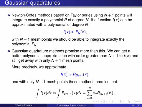
Gaussian quadratures
Newton-Cotes methods based on Taylor series using N + 1 points willintegrate exactly a polynomial P of degree N. If a function f (x) can beapproximated with a polynomial of degree N
f (x) ≈ PN(x),
with N + 1 mesh points we should be able to integrate exactly thepolynomial PN .
Gaussian quadrature methods promise more than this. We can get abetter polynomial approximation with order greater than N + 1 to f (x) andstill get away with only N + 1 mesh points.
More precisely, we approximate
f (x) ≈ P2N+1(x),
and with only N + 1 mesh points these methods promise that∫f (x)dx ≈
∫P2N+1(x)dx =
N∑i=0
wiP2N+1(xi ),
TFY4235/FYS8904 Computational Physics – ver2018 281 / 515

Gaussian Quadratures
A quadrature formula ∫ b
aW (x)f (x)dx ≈
N∑i=0
wi f (xi ),
with N + 1 distinct quadrature points (mesh points) is a called a Gaussianquadrature formula if it integrates all polynomials p ∈ P2N+1 exactly, that is∫ b
aW (x)p(x)dx =
N∑i=0
wip(xi ),
It is assumed that W (x) is continuous and positive and that the integral∫ b
aW (x)dx
exists. Note that the replacement of f →Wg is normally a betterapproximation due to the fact that we may isolate possible singularities of Wand its derivatives at the endpoints of the interval.
TFY4235/FYS8904 Computational Physics – ver2018 282 / 515

Gaussian quadratures
But which xi and wi to use?
The theoretical foundation behind Gaussian quadratures is interesting,but will not be covered here!
The abscissas xi are related to othogonal polynomials (e.g. Legendrepolynomials) in the sense that they are the zeroes for these polynomials
The weights wi are determined so that the integrator is exact for apolynomial up to a given order
Library routines give you the sets wi and xi for a given Gaussianquadrature
The homepage of John Burkardt offers many of these and other routines:http://people.sc.fsu.edu/˜jburkardt/
TFY4235/FYS8904 Computational Physics – ver2018 283 / 515
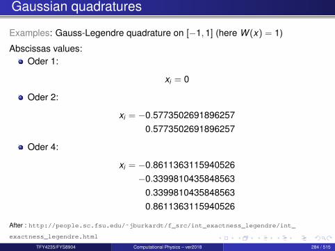
Gaussian quadratures
Examples: Gauss-Legendre quadrature on [−1,1] (here W (x) = 1)
Abscissas values:Oder 1:
xi = 0
Oder 2:
xi = −0.57735026918962570.5773502691896257
Oder 4:
xi = −0.8611363115940526−0.3399810435848563
0.33998104358485630.8611363115940526
After : http://people.sc.fsu.edu/˜jburkardt/f_src/int_exactness_legendre/int_
exactness_legendre.html
TFY4235/FYS8904 Computational Physics – ver2018 284 / 515

Gaussian quadratures
Examples: Gauss-Legendre quadrature on [−1,1] (not equidistant sampling)
After : http://people.sc.fsu.edu/˜jburkardt/f_src/int_exactness_legendre/int_
exactness_legendre.html
TFY4235/FYS8904 Computational Physics – ver2018 285 / 515
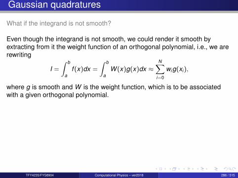
Gaussian quadratures
What if the integrand is not smooth?
Even though the integrand is not smooth, we could render it smooth byextracting from it the weight function of an orthogonal polynomial, i.e., we arerewriting
I =
∫ b
af (x)dx =
∫ b
aW (x)g(x)dx ≈
N∑i=0
wig(xi ),
where g is smooth and W is the weight function, which is to be associatedwith a given orthogonal polynomial.
TFY4235/FYS8904 Computational Physics – ver2018 286 / 515

Gaussian quadratures
The weight function W is non-negative in the integration interval x ∈ [a,b]
such that for any N ≥ 0,∫ b
a |x |NW (x)dx is integrable.
The naming weight function arises from the fact that it may be used togive more emphasis to one part of the interval than another.
Weight function Interval PolynomialW (x) = 1 x ∈ [a,b] LegendreW (x) = e−x2 −∞ ≤ x ≤ ∞ HermiteW (x) = e−x 0 ≤ x ≤ ∞ LaguerreW (x) = 1/(
√1− x2) −1 ≤ x ≤ 1 Chebyshev
TFY4235/FYS8904 Computational Physics – ver2018 287 / 515
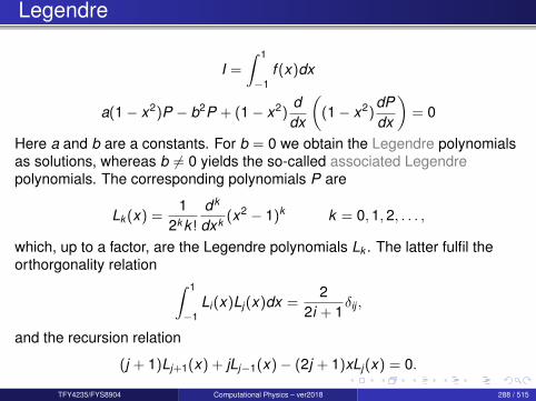
Legendre
I =
∫ 1
−1f (x)dx
a(1− x2)P − b2P + (1− x2)ddx
((1− x2)
dPdx
)= 0
Here a and b are a constants. For b = 0 we obtain the Legendre polynomialsas solutions, whereas b 6= 0 yields the so-called associated Legendrepolynomials. The corresponding polynomials P are
Lk (x) =1
2k k !
dk
dxk (x2 − 1)k k = 0,1,2, . . . ,
which, up to a factor, are the Legendre polynomials Lk . The latter fulfil theorthorgonality relation ∫ 1
−1Li (x)Lj (x)dx =
22i + 1
δij ,
and the recursion relation
(j + 1)Lj+1(x) + jLj−1(x)− (2j + 1)xLj (x) = 0.
TFY4235/FYS8904 Computational Physics – ver2018 288 / 515
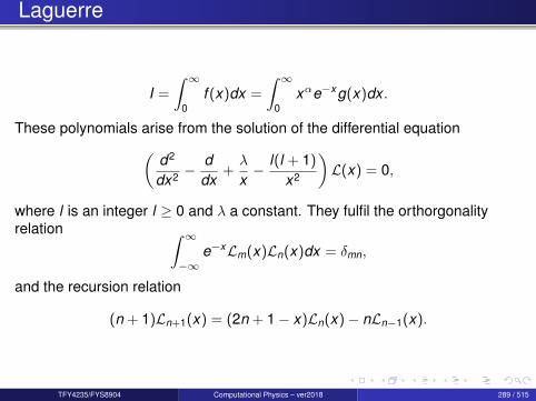
Laguerre
I =
∫ ∞0
f (x)dx =
∫ ∞0
xαe−xg(x)dx .
These polynomials arise from the solution of the differential equation(d2
dx2 −ddx
+λ
x− l(l + 1)
x2
)L(x) = 0,
where l is an integer l ≥ 0 and λ a constant. They fulfil the orthorgonalityrelation ∫ ∞
−∞e−xLm(x)Ln(x)dx = δmn,
and the recursion relation
(n + 1)Ln+1(x) = (2n + 1− x)Ln(x)− nLn−1(x).
TFY4235/FYS8904 Computational Physics – ver2018 289 / 515
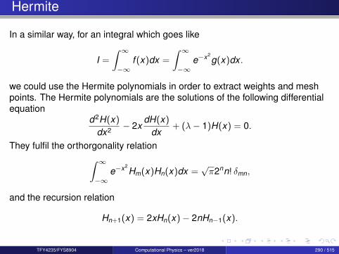
Hermite
In a similar way, for an integral which goes like
I =
∫ ∞−∞
f (x)dx =
∫ ∞−∞
e−x2g(x)dx .
we could use the Hermite polynomials in order to extract weights and meshpoints. The Hermite polynomials are the solutions of the following differentialequation
d2H(x)
dx2 − 2xdH(x)
dx+ (λ− 1)H(x) = 0.
They fulfil the orthorgonality relation∫ ∞−∞
e−x2Hm(x)Hn(x)dx =
√π2nn! δmn,
and the recursion relation
Hn+1(x) = 2xHn(x)− 2nHn−1(x).
TFY4235/FYS8904 Computational Physics – ver2018 290 / 515

Some examples
Integral : Evaluate the integral∫ 3
0dx
12 + x2 =
1√2
arctan(√
18/4)≈ 0.7992326575 . . .
Results :
N Trapezoidal Simpson Gauss-Legendre10 0.798861 0.799231 0.79923320 0.799140 0.799233 0.79923340 0.799209 0.799233 0.799233
100 0.799229 0.799233 0.7992331000 0.799233 0.799233 0.799233
Python : Calculate the integral over f (x) from a to b viascipy.integrate.quadrature(f,a,b)scipy.integrate.quad(f,a,b)
TFY4235/FYS8904 Computational Physics – ver2018 291 / 515
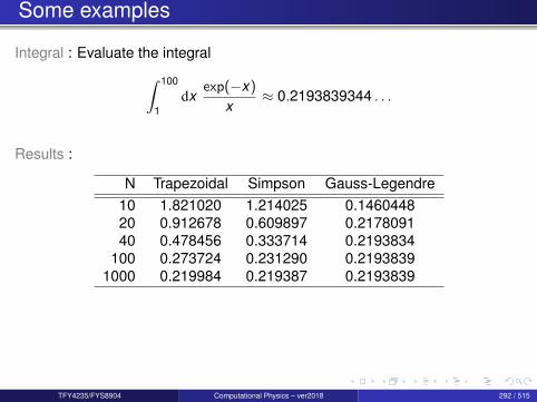
Some examples
Integral : Evaluate the integral∫ 100
1dx
exp(−x)
x≈ 0.2193839344 . . .
Results :
N Trapezoidal Simpson Gauss-Legendre10 1.821020 1.214025 0.146044820 0.912678 0.609897 0.217809140 0.478456 0.333714 0.2193834
100 0.273724 0.231290 0.21938391000 0.219984 0.219387 0.2193839
TFY4235/FYS8904 Computational Physics – ver2018 292 / 515
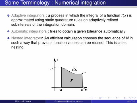
Some Terminology : Numerical integration
Adaptive integrators : a process in which the integral of a function f (x) isapproximated using static quadrature rules on adaptively refinedsubintervals of the integration domain.
Automatic integrators : tries to obtain a given tolerance automatically
Nested integrators: An efficient calculation chooses the sequence of N insuch a way that previous function values can be reused. This is callednesting.
TFY4235/FYS8904 Computational Physics – ver2018 293 / 515

Quadratures not discussed
Gauss-Kronrod quadraturea variant of Gaussian quadrature, in which the evaluation points arechosen so that an accurate approximation can be computed by re-usingthe information produced by the computation of a less accurateapproximation, i.e. Gauss-Kronrod quadrature are nested.
Clenshaw-Curtis quadrature (Fejer quadratures)Based on an expansion of the integrand in terms of Chebyshevpolynomials. A change of variables x = cos θ is done and a discretecosine transform (DCT) is used to calculate the resulting series.Clenshaw-Curtis quadrature naturally leads to nested quadrature rules.Special Clenshaw-Curtis quadratures exist for integrands W (x)f (x) witha weight function W (x) that is highly oscillatory, e.g. a sinusoid or Besselfunctions. These methods are useful for high-accuracy integration ofrapid oscillating integrands.
Due to the nested nature of the Gauss-Kronrod and Clenshaw-Curtisquadratures they are frequently used for adaptive quadratures!
TFY4235/FYS8904 Computational Physics – ver2018 294 / 515
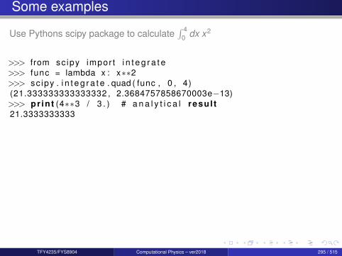
Some examples
Use Pythons scipy package to calculate∫ 4
0 dx x2
>>> from sc ipy impor t i n t e g r a t e>>> func = lambda x : x∗∗2>>> sc ipy . i n t e g r a t e . quad ( func , 0 , 4)(21.333333333333332 , 2.3684757858670003e−13)>>> pr in t (4∗∗3 / 3 . ) # a n a l y t i c a l resul t21.3333333333
TFY4235/FYS8904 Computational Physics – ver2018 295 / 515
Romberg quadrature
Romberg integration is a powerful methodIt consists of repeatably using an integrator for stepsizes, say, h, h/2, h/4etc. and than extrapolating to h→ 0Romberg integration is “Richardson extrapolation” (a sequenceacceleration method) applied to integrationRomberg was a professor in Trondheim (NTH)
Example: see e.g.https://en.wikipedia.org/wiki/Romberg%27s_method
TFY4235/FYS8904 Computational Physics – ver2018 296 / 515
Ways of increasing integration accuracy
Question : How can one increase the accuracy of a numerical integration?
Increasing the number of points (not always a good idea, why not?)Using a more accurate integratorUsing subdivision of the integration domainUsing an automatic adaptive integrator (which typically uses subdivision)
We will now look at some of these possibilities!
TFY4235/FYS8904 Computational Physics – ver2018 297 / 515
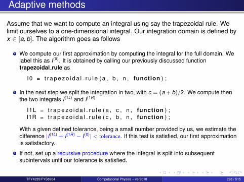
Adaptive methods
Assume that we want to compute an integral using say the trapezoidal rule. Welimit ourselves to a one-dimensional integral. Our integration domain is defined byx ∈ [a,b]. The algorithm goes as follows
We compute our first approximation by computing the integral for the full domain. Welabel this as I(0). It is obtained by calling our previously discussed functiontrapezoidal rule as
I0 = t r a p e z o i d a l r u l e ( a , b , n , function ) ;
In the next step we split the integration in two, with c = (a + b)/2. We compute thenthe two integrals I(1L) and I(1R)
I1L = t r a p e z o i d a l r u l e ( a , c , n , function ) ;I1R = t r a p e z o i d a l r u l e ( c , b , n , function ) ;
With a given defined tolerance, being a small number provided by us, we estimate thedifference |I(1L) + I(1R) − I(0)| < tolerance. If this test is satisfied, our first approximationis satisfactory.
If not, set up a recursive procedure where the integral is split into subsequentsubintervals until our tolerance is satisfied.
TFY4235/FYS8904 Computational Physics – ver2018 298 / 515
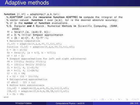
Adaptive methods
function [ I , n f ] = adaptsimp ( f , a , b , t o l ) ;% ADAPTSIMP c a l l s the recursive function ADAPTREC to compute the i n t e g r a l o f the% vector−valued function f over [ a , b ] ; t o l i s the des i red absolu te accuracy ;% nf i s the number of function eva lua t ions .% G. Da lqu i s t and A Bjorck , Numerical Methods in S c i e n t i f i c Computing , (SIAM ,
2008) .f f = f e v a l ( f , [ a , ( a+b ) / 2 , b ] ) ;n f = 3 ; % I n i t i a l Simpson approximat ionI1 = ( b − a ) ∗ [ 1 , 4 , 1 ]∗ f f ’/6;% Recursive computation[I,nf] = adaptrec(f,a,b,ff,I1,tol,nf);function [I,nf] = adaptrec(f,a,b,ff,I1,tol,nf);h = (b - a)/2;fm = feval(f, [a + h/2, b - h/2]);nf = nf + 2;% Simpson approximations for left and right subintervalfR = [ff(2); fm(2); ff(3)];fL = [ff(1); fm(1); ff(2)];IL = h*[1, 4, 1]*fL/6;IR = h*[1, 4, 1]*fR/6;I2 = IL + IR;I = I2 + (I2 - I1)/15;% Extrapolated approximationif abs(I - I2) > tol% Refine both subintervals[IL,nf] = adaptrec(f,a,a+h,fL,IL,tol/2,nf);[IR,nf] = adaptrec(f,b-h,b,fR,IR,tol/2,nf);I = IL + IR;
end
TFY4235/FYS8904 Computational Physics – ver2018 299 / 515

Adaptive methods
Example: Use the MATLAB routine adaptsimp to integrate
I =
∫ 4
−4
dx1 + x2 = 2.65163532733607.
Results
I tolerance n Error2.6516250211 10−4 41 1.0 10−5
2.6516352064 10−5 81 1.2 10−7
2.651635327353 10−6 153 −1.7 10−11
Here n is the no. of function calls.
TFY4235/FYS8904 Computational Physics – ver2018 300 / 515

Adaptive methods
The recommended canned integration routines are typically adaptive
For instance, QAGS from QUADPACK uses an adaptive Gauss-Kronrodquadratures, and it is the main routine used in
scipy.integrate.quadMatlab/Octave : quadGSL: gsl integration qags
TFY4235/FYS8904 Computational Physics – ver2018 301 / 515
Numerical integration one-dimension:Recommendations
The general recommendation I would give for numerical integration is:
Adaptive Gauss-Kronrod or Clenshaw-Curtis quadratures if f (x) is knowfor any argument x
e.g. QAGS from quadpack (available through various libraries)
Newton-Cotes if f (x) is tabulated
TFY4235/FYS8904 Computational Physics – ver2018 302 / 515
Software: One-dimensional numerical integration
The following software packages provide numerical integration routines:
QUADPACK library (part of Slatec)http://en.wikipedia.org/wiki/QUADPACK
GNU Scientific Library (contains QUADPACK)Boost C++ libraries www.boost.org/Python scipyNAG Numerical Libraries (commercial)
Another good source isJohn Burkardt homepage:http://people.sc.fsu.edu/˜jburkardt/
TFY4235/FYS8904 Computational Physics – ver2018 303 / 515

Software: QUADPACK
QAGS: uses global adaptive quadrature based on 21-pointGauss-Kronrod quadrature within each subinterval, with acceleration byPeter Wynn’s epsilon algorithm
QAGI: is the only general-purpose routine for infinite intervals, and mapsthe infinite interval onto the semi-open interval (0,1] using atransformation that uses the same approach as QAGS, except with15-point rather than 21-point Gauss-Kronrod quadrature.
For an integral over the whole real line, the transformation used isx = (1− t)/t∫ +∞
−∞f (x)dx =
∫ 1
0
dtt2
[f(
1− tt
)+ f(−1− t
t
)].
QUADPACK also contains routines for singular integrands (QAGP), andCauchy principle value integrals (QAWC) (to be discussed next)
See : http://en.wikipedia.org/wiki/QUADPACKTFY4235/FYS8904 Computational Physics – ver2018 304 / 515
Numerical integration of singular integrands
Question : How can one evaluate the integral
I(a,b) =
∫ b
adx f (x)
if f (x) has a singularity in the interval [a,b]?
First question to ask:where is the singularity locatedwhat kind of singularity; algebraic, logarithmic, etc.
Various approaches:“ignore” the singularity (not in general a good idea)specially designed Gaussian quadrature handling the singularity as aweighting function“transformation trick”: transform it away analytically“subtraction trick”: subtract off the singularity and treat it analytically
TFY4235/FYS8904 Computational Physics – ver2018 305 / 515
Numerical integration of singular integrands
Numerical integration of singular integrands, may, or-may-not, be donesuccessfully with a normal quadrature rule if we avoid the singular point.
However, we stress such strategy may not be successful, so real care shouldbe taken. For instance for oscillatory integrands, the method of “ignoring thesingularity” does not work well.
Homework: Try this approach to the integrals (eg. using Simpson and/orGauss-Legendre quadratures)
Integral 1
I1 =
∫ 1
0dx
1√x
= 2
Integral 2
I2 =
∫ 1
0dx
1x
sin
(1x
)= 0.624713 . . .
TFY4235/FYS8904 Computational Physics – ver2018 306 / 515
Numerical integration of singular integrands
First advice : investigate if one can transform or modify the given problemanalytically to make it more suitable for numerical integration
Example 1: Numerically calculate (singularity at x = 0)
I =
∫ 1
0dx
ex√
x
However, make a change of variable x = t2, to get
I = 2∫ 1
0dt exp(t2)
which is well-behaved.
Alternatively one may do a few integrations by part!
TFY4235/FYS8904 Computational Physics – ver2018 307 / 515

Numerical integration of singular integrands
Alternatively one may construct a special Newton-Cotes rule the integral withweight function W (x) = 1/
√x∫ 2h
0dx
f (x)√x≈√
2h [w0f (0) + w1f (h) + w2f (2h)] .
Using the method of undetermined coefficients for polynomials f (x) = 1, x , x2
gives ∫ 2h
0dx
f (x)√x≈√
2h[
1215
f (0) +1615
f (h) +2
15f (2h)
].
Show this yourself!
TFY4235/FYS8904 Computational Physics – ver2018 308 / 515
Numerical integration of singular integrands
Example 2: A more general form
Numerically calculate for f (x) ∈ C[0,1]
I =
∫ 1
0dx
f (x)
x1/α , α ≥ 2
Here a change of variable x = tα results in
I = α
∫ 1
0dt tα−2f (tα)
which is also well-behaved and better suited for numerical evaluation.
TFY4235/FYS8904 Computational Physics – ver2018 309 / 515

Numerical integration of singular integrands
Example 3: What to do with this integral for f (x) ∈ C[0,1]
I =
∫ 1
0dx ln(x)f (x)
Question: What to do here regarding the logarithmic singularity at x = 0?
TFY4235/FYS8904 Computational Physics – ver2018 310 / 515

Numerical integration of singular integrands
Example 3: What to do with this integral for f (x) ∈ C[0,1]
I =
∫ 1
0dx ln(x)f (x)
Question: What to do here regarding the logarithmic singularity at x = 0?
Possible answer : A change of variable x = e−t , will do the job since it implies
I = −∫ ∞
0dt te−t f (e−t )
which is a well behaved improper integral (that can be transformed to a finiteintegration domain).
TFY4235/FYS8904 Computational Physics – ver2018 311 / 515
Numerical integration of singular integrands
Second advice : If the singular points are known, but can not betransformed away, then the integral should first be broken up into severalpieces so that all the singularities are located at one (or both) ends of theinterval [a,b].
Say we have a singularity at c ∈ [a,b], then do∫ b
adx f (x) =
∫ c
adx f (x) +
∫ b
cdx f (x)
Many integrals can then be treated by weighted quadrature rules, i.e., thesingularity is incorporated into the weight function
Comments: Many canned integration routines, like QAGS from QUADPACK,do this for you automatically!
TFY4235/FYS8904 Computational Physics – ver2018 312 / 515
Numerical integration of singular integrands
Elimination of the singularity by subtracting it off and treat it analytically
Consider again the integral
I =
∫ b
adx f (x)
where f (x) has an integrable singularity in [a,b] that can not be transformedaway. Assume that g(x) has a similar behavior to f (x) around the singularity.
Then do
I =
∫ b
adx g(x) +
∫ b
adx [f (x)− g(x)] ≡ IA + IN
where IA is treated analytically, and IN numerically since it does not have asingularity.
This methods only works if a function g(x) can be found that allows ananalytic treatment.
TFY4235/FYS8904 Computational Physics – ver2018 313 / 515
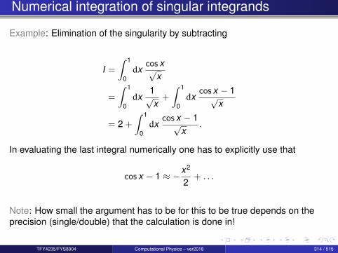
Numerical integration of singular integrands
Example: Elimination of the singularity by subtracting
I =
∫ 1
0dx
cos x√x
=
∫ 1
0dx
1√x
+
∫ 1
0dx
cos x − 1√x
= 2 +
∫ 1
0dx
cos x − 1√x
.
In evaluating the last integral numerically one has to explicitly use that
cos x − 1 ≈ −x2
2+ . . .
Note: How small the argument has to be for this to be true depends on theprecision (single/double) that the calculation is done in!
TFY4235/FYS8904 Computational Physics – ver2018 314 / 515
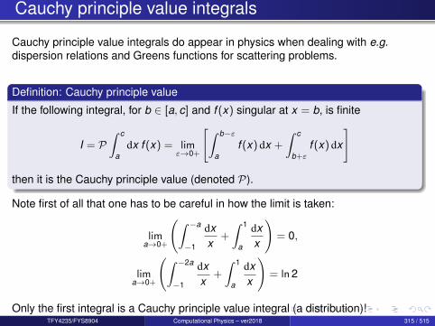
Cauchy principle value integrals
Cauchy principle value integrals do appear in physics when dealing with e.g.dispersion relations and Greens functions for scattering problems.
Definition: Cauchy principle value
If the following integral, for b ∈ [a, c] and f (x) singular at x = b, is finite
I = P∫ c
adx f (x) = lim
ε→0+
[∫ b−ε
af (x) dx +
∫ c
b+ε
f (x) dx
]
then it is the Cauchy principle value (denoted P).
Note first of all that one has to be careful in how the limit is taken:
lima→0+
(∫ −a
−1
dxx
+
∫ 1
a
dxx
)= 0,
lima→0+
(∫ −2a
−1
dxx
+
∫ 1
a
dxx
)= ln 2
Only the first integral is a Cauchy principle value integral (a distribution)!TFY4235/FYS8904 Computational Physics – ver2018 315 / 515
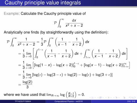
Cauchy principle value integrals
Example: Calculate the Cauchy principle value of
P∫ ∞
0
dxx2 + x − 2
Analytically one finds (by straightforwardly using the definition):
P∫ ∞
0
1x2 + x − 2
=13P∫ ∞
0
(1
x − 1− 1
x + 2
)dx
=13
limε→0
[∫ 1−ε
0
(1
x − 1− 1
x + 2
)dx +
∫ ∞1+ε
(1
x − 1− 1
x + 2
)dx
]
=13
limε→0
[[log(1− x)− log(x + 2)]1−ε0 + [log(x − 1)− log(x + 2)]∞1+ε
]=
13
limε→0
[log(ε)− log(3− ε) + log(2)− log(ε) + log(3 + ε)]
=log(2)
3
where we have used that limR→∞ log(
R−1R+2
)= 0.
TFY4235/FYS8904 Computational Physics – ver2018 316 / 515
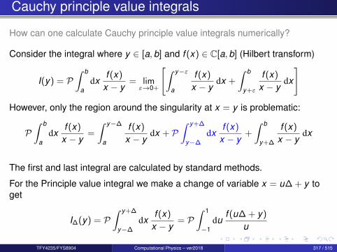
Cauchy principle value integrals
How can one calculate Cauchy principle value integrals numerically?
Consider the integral where y ∈ [a,b] and f (x) ∈ C[a,b] (Hilbert transform)
I(y) = P∫ b
adx
f (x)
x − y= limε→0+
[∫ y−ε
a
f (x)
x − ydx +
∫ b
y+ε
f (x)
x − ydx
]However, only the region around the singularity at x = y is problematic:
P∫ b
adx
f (x)
x − y=
∫ y−∆
a
f (x)
x − ydx + P
∫ y+∆
y−∆
dxf (x)
x − y+
∫ b
y+∆
f (x)
x − ydx
The first and last integral are calculated by standard methods.
For the Principle value integral we make a change of variable x = u∆ + y toget
I∆(y) = P∫ y+∆
y−∆
dxf (x)
x − y= P
∫ 1
−1du
f (u∆ + y)
u
TFY4235/FYS8904 Computational Physics – ver2018 317 / 515

Cauchy principle value integrals
Now we use the “subtraction trick” to calculate I∆(y)
I∆(y) = P∫ 1
−1du[
f (u∆ + y)− f (y)
u+
f (y)
u
]= P
∫ 1
−1du[
f (u∆ + y)− f (y)
u
]+ f (y)P
∫ 1
−1du
1u︸ ︷︷ ︸
0
=
∫ 1
−1du[
f (u∆ + y)− f (y)
u
]where we in the last transition have taken advantage of the integrand nolonger is singular since
limu→0
[f (∆u + y)− f (y)] = 0
Calculate I∆(y) by Gauss-Legendre quadratures of EVEN order (why?)
TFY4235/FYS8904 Computational Physics – ver2018 318 / 515
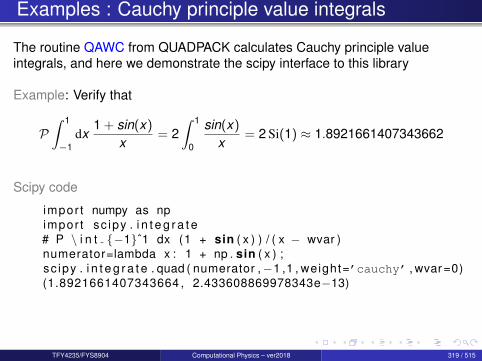
Examples : Cauchy principle value integrals
The routine QAWC from QUADPACK calculates Cauchy principle valueintegrals, and here we demonstrate the scipy interface to this library
Example: Verify that
P∫ 1
−1dx
1 + sin(x)
x= 2
∫ 1
0
sin(x)
x= 2 Si(1) ≈ 1.8921661407343662
Scipy code
impor t numpy as npimpor t sc ipy . i n t e g r a t e# P \ i n t −1ˆ1 dx (1 + sin ( x ) ) / ( x − wvar )numerator=lambda x : 1 + np . sin ( x ) ;sc ipy . i n t e g r a t e . quad ( numerator ,−1 ,1 , weight=’cauchy’ , wvar=0)(1.8921661407343664 , 2.433608869978343e−13)
TFY4235/FYS8904 Computational Physics – ver2018 319 / 515

Multidimensional integrals
The multidimensional integral
In(a,b) =
∫ b1
a1
dx1
∫ b2
a2
dx2 . . .
∫ bn
an
dxn f (x)
can be calculated as repeated one-dimensional integralsThis is valid for any numerical integration methodNumerical integration over more than one dimension is sometimesdescribed as “cubatures”Different integration methods can be applied in different dimensions
Challenge: “Curse of dimensionality”The exponentially rising cost associated with simple product grids
Ex: With 106 function eval. leaves about 2 points per direction in 20D!
This cost is unaffordable, but worse, it is unnecessary !
TFY4235/FYS8904 Computational Physics – ver2018 320 / 515

Sparse grid methods —Smolyak quadratures
Sparse grids avoid the exponentially rising cost associated with simpleproduct grids, and can produce more accurate results than a Monte Carloapproach if the function has bounded derivatives of sufficient order.
Tensor product grid Sparse grid
TFY4235/FYS8904 Computational Physics – ver2018 321 / 515

Sparse grid methods — Smolyak quadratures
developed by the Russian mathematician Sergey A. Smolyakbased on a sparse tensor product constructionSmolyak’s quadrature rule : more efficient method of integratingmultidimensional functionsSparse Grid = Sum of Selected Product Rule (more efficient)
Tutorial: http://www.math.tu-berlin.de/˜garcke/paper/sparseGridTutorial.pdf
Software http://people.sc.fsu.edu/˜jburkardt
TFY4235/FYS8904 Computational Physics – ver2018 322 / 515

Monte-Carlo integration
Trivial example : Calculate π by random numbers!
π = 4AA
= 4 limN→∞
NN
TFY4235/FYS8904 Computational Physics – ver2018 323 / 515
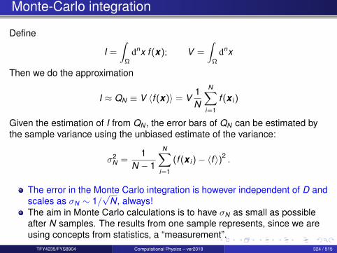
Monte-Carlo integration
Define
I =
∫Ω
dnx f (x); V =
∫Ω
dnx
Then we do the approximation
I ≈ QN ≡ V 〈f (x)〉 = V1N
N∑i=1
f (x i )
Given the estimation of I from QN , the error bars of QN can be estimated bythe sample variance using the unbiased estimate of the variance:
σ2N =
1N − 1
N∑i=1
(f (x i )− 〈f 〉)2.
The error in the Monte Carlo integration is however independent of D andscales as σN ∼ 1/
√N, always!
The aim in Monte Carlo calculations is to have σN as small as possibleafter N samples. The results from one sample represents, since we areusing concepts from statistics, a “measurement”.
TFY4235/FYS8904 Computational Physics – ver2018 324 / 515

The volume of an n-dimensional sphere
The n-dimensional sphere of radius R, the “Euclidean ball”, is the volumebounded by the surface |x | = R where x ∈ Rn.The volume of such a sphere is
Vn(R) =
∫|x |<R
dnx
Homework: Calculate the volume Vn(R) for different values of n ∈ N0!
TFY4235/FYS8904 Computational Physics – ver2018 325 / 515
Section 9
Random numbers
TFY4235/FYS8904 Computational Physics – ver2018 326 / 515

Outline I
1 Introduction
2 Number representation and numerical precision
3 Finite differences and interpolation
4 Linear algebra
5 How to install libraries on a Linux system
6 Eigenvalue problems
7 Spectral methods
8 Numerical integration
TFY4235/FYS8904 Computational Physics – ver2018 327 / 515

Outline II9 Random numbers
Uniform pseudo random number generatorsNonuniform pseudo random number generators
10 Ordinary differential equations
11 Partial differential equations
12 Optimization
TFY4235/FYS8904 Computational Physics – ver2018 328 / 515
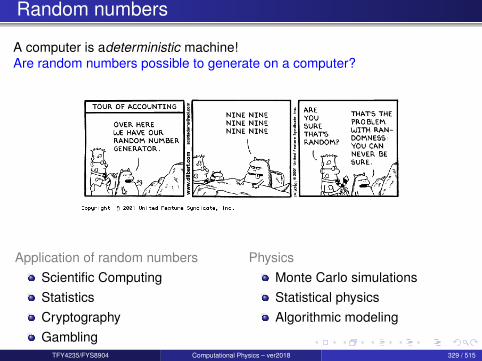
Random numbers
A computer is adeterministic machine!Are random numbers possible to generate on a computer?
Application of random numbersScientific ComputingStatisticsCryptographyGambling
PhysicsMonte Carlo simulationsStatistical physicsAlgorithmic modeling
TFY4235/FYS8904 Computational Physics – ver2018 329 / 515
Random numbers
Use of Random Number Generators (RNGs)
In principle, RNGs are needed in any application where unpredictable resultsare required.
For most applications it is desirable to have fast RNGs that producenumbers that are as random as possibleHowever, these two properties are often inversely proportional to eachotherExcellent RNGs are often slow, whereas poor RNGs are typically fast
Good introduction :Helmut G. Katzgraber, Random Numbers in Scientific Computing: An Introduction,arXiv:1005.4117, 2010; http://arxiv.org/abs/1005.4117
TFY4235/FYS8904 Computational Physics – ver2018 330 / 515
Random numbers
Main classes of RNGs:
True RNGsTrue random numbers are generatedThere are no correlations in the sequence of numbers
special hardware typically needed (exception /dev/random)True RNGs are generally slow; limited use for large-scale computer simul.Debugging difficult; No restart of the sequence
Buy random numbers from www.random.org/
Pseudo RNGs (PRNGs)are fast (no need for post-processing)do not require special hardware and therefore are very portableeasy debugging: the exact sequence of RNs may be reproduced
have finite sequence lengthsthe numbers produced may be correlated (i.e. know your generator!)
TFY4235/FYS8904 Computational Physics – ver2018 331 / 515
Pseudo Random Number Generators
Good pseudo RNGs should beRandomReproduciblePortableEfficient
Random numbers from any distribution, takes uniform random numbers,denoted U(0,1), as the starting point.
No universal PRNG!There is NO universal pseudo random number generator (PRNG).Always test your PRNG in the application you have in mind!
The field of PRNGs is evolving quickly;A generator that was considered good in the past, may no longer be “good”.
TFY4235/FYS8904 Computational Physics – ver2018 332 / 515
Uniform deviates; U(0,1)
Algorithm: Uniform PRNGs
Generate a sequence of numbers x1, x2 ,x3, . . ., using a recurrence of the form
xi = f (xi−1, xi−2, . . . , xi−n)
where n initial numbers (seed block) are needed to start the recurrence.
All PRNGs have this structure; the magic lies in finding a function f (·) thatproduces numbers that are “as random as possible”.The initial values — the seed — determines the sequence of randomnumbers.
Methods for generating uniform pseudo random numbers U(0,1):Linear congruential generatorsLagged Fibonacci generatorsOther commonly-used PRNGs
TFY4235/FYS8904 Computational Physics – ver2018 333 / 515
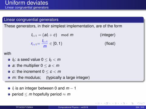
Uniform deviatesLinear congruential generators
Linear congruential generators
These generators, in their simplest implementation, are of the form
Ii+1 = (aIi + c) mod m (integer)
ri+1=Ii+1
m∈ [0,1) (float)
withI0: a seed value 0 ≤ I0 < ma: the multiplier 0 ≤ a < mc: the increment 0 ≤ c < mm: the modulus; (typically a large integer)
Ii is an integer between 0 and m − 1period ≤ m hopefully period ≈ m
TFY4235/FYS8904 Computational Physics – ver2018 334 / 515

Uniform deviatesLinear congruential generators
The choice of constants (I0,a, c,m) influence the quality of the generatorMathematicians have partly guided us how to pick “magic numbers”sequential correlations show upPark-Miller generator : c = 0
Some choices:“Minimal Standard Generator” (Lewis, Goodman and Miller (1969))
a = 16 807; c = 0; and m = 231 − 1 = 2147483647 ∼ 109 [using 32-bitsinteger]good for generating unsigned 32-bit random integersvery fast and full period of 231 − 1 ∼ 109 (often too short for floats)little sequential correlations
drand48( )a = 25214903917, c = 11 and m = 248 ∼ 1014
TFY4235/FYS8904 Computational Physics – ver2018 335 / 515
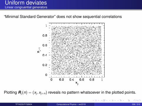
Uniform deviatesLinear congruential generators
“Minimal Standard Generator” does not show sequential correlations
Plotting R j (n) = (xj , xj+n) reveals no pattern whatsoever in the plotted points.
TFY4235/FYS8904 Computational Physics – ver2018 336 / 515
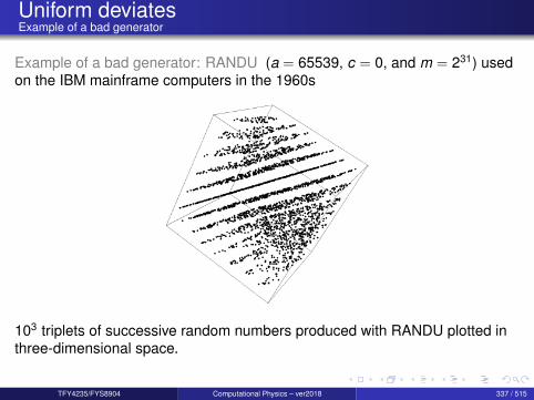
Uniform deviatesExample of a bad generator
Example of a bad generator: RANDU (a = 65539, c = 0, and m = 231) usedon the IBM mainframe computers in the 1960s
103 triplets of successive random numbers produced with RANDU plotted inthree-dimensional space.
TFY4235/FYS8904 Computational Physics – ver2018 337 / 515
Uniform deviatesLagged Fibonacci generators
Lagged Fibonacci generators
These generators are of the form
xi = (xi−j xi−k ) mod m, 0 < j < k ,
where denotes a binary operator, i.e. addition, multiplication or exclusiveOR (XOR; “one or the other but not both”)
Typically m = 2M with M = 32 or 64.Requires a seed block of size k to be initialized (often with a Linearcongruential generator)When is a multiplication [addition] one talks about multiplicative[additative] lagged Fibonacci generators
The name derives from the similarity to the Fibonacci series
xi = xi−1 + xi−2 → 1,1,2,3,5,8,13,21, . . .
TFY4235/FYS8904 Computational Physics – ver2018 338 / 515

Uniform deviatesLagged Fibonacci generators
Lagged Fibonacci generators are intended as an improvement over linear congruentialgenerators and, in general, they are not only fast but most of them pass all standardempirical random number generator tests.
Examples of Lagged Fibonacci generators are
r1279()
multiplicative generator with k = 1279period approximately 10394
has passed all known PRNG teststhe “standard” generator in e.g. GNU Scientific Library
r250(); not a so good generator!k = 250; = XORFor many years the “standard generator” in numerical simulations
Problem: Energy per spin in the Ising model at the critical temperature wasapproximately 42 standard deviations off the known exact result (1992)
TFY4235/FYS8904 Computational Physics – ver2018 339 / 515

Uniform deviatesOther generators
Mersenne Twister; mt19937(), mt19937-64()
Developed in 1997, and passed almost all known testsamong the most frequently used generators of todayfast generatorPeriod 219937 − 1 ≈ 106001
period determined by Mersenne primes (Mn = 2n − 1, n ∈ N)available in 32 and 64-bits architecturesavailable in C/C++, Fortran, GSL, Matlab, Python, Boost etc.en.wikipedia.org/wiki/Mersenne_twister
WELL generators — Well Equidistributed Long-period Linearoriginally developed by Panneton, L’Ecuyer and MatsumotoThe idea is to provide better equidistribution and bit mixing with anequivalent period length and speed as the Mersenne Twister
TFY4235/FYS8904 Computational Physics – ver2018 340 / 515

How to test the quality of PRNGs?
Various different test suites have been developed with the sole purpose oftesting PRNGs.
Simple tests for N PRNs from U(0,1)
correlation test : 〈xixi+n〉 − 〈x〉2 < O(1/√
N)moment test :
⟨xk⟩− 1/(k + 1) < O(1/
√N)
Graphical test : plot R i = (xi , xi+1) etc.
DIEHARD by George Marsagliaconsists of 16 different testsFor more details visithttp://en.wikipedia.org/wiki/Diehard_tests
There is NO ultimate test!Therefore run your code with different PRNGs.If the results agree within error bars and the PRNGs used are from differentfamilies, the results are likely to be trusted.
TFY4235/FYS8904 Computational Physics – ver2018 341 / 515
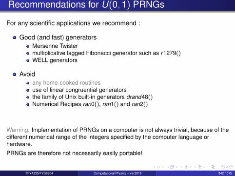
Recommendations for U(0,1) PRNGs
For any scientific applications we recommend :
Good (and fast) generatorsMersenne Twistermultiplicative lagged Fibonacci generator such as r1279()WELL generators
Avoidany home-cooked routinesuse of linear congruential generatorsthe family of Unix built-in generators drand48()Numerical Recipes ran0(), ran1() and ran2()
Warning: Implementation of PRNGs on a computer is not always trivial, because of thedifferent numerical range of the integers specified by the computer language orhardware.
PRNGs are therefore not necessarily easily portable!
TFY4235/FYS8904 Computational Physics – ver2018 342 / 515

Final recommendations
Dealing with random numbers can be a delicate issue. Therefore. . .
Always try to run your simulations with two different PRNGs from differentfamilies, at least for small testing instances. One option would be to usean excellent but slow PRNG versus a very good but fast PRNG. For theproduction runs then switch to the fast one.To ensure data provenance always store the information of the PRNG aswell as the seed used (better even the whole code) with the data. Thiswill allow others to reproduce your results.Use trusted PRNG implementations. As much as it might feel good tomake your own PRNG, rely on those who are experts in creating thesedelicate generators.Know your PRNG’s limits: How long is the period? Are there knownproblems for certain applications? Are there correlations at any timeduring the sequence?Be careful with parallel simulations.
Recommendations from : http://arxiv.org/abs/1005.4117
TFY4235/FYS8904 Computational Physics – ver2018 343 / 515
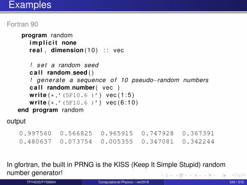
Examples
Fortran 90
program randomi m p l i c i t nonereal , dimension (10) : : vec
! se t a random seedc a l l random seed ( )! generate a sequence of 10 pseudo−random numbersc a l l random number ( vec )write (∗ ,’(5F10.6 )’ ) vec ( 1 : 5 )write (∗ ,’(5F10.6 )’ ) vec ( 6 : 1 0 )
end program random
output
0.997560 0.566825 0.965915 0.747928 0.3673910.480637 0.073754 0.005355 0.347081 0.342244
In gfortran, the built in PRNG is the KISS (Keep It Simple Stupid) randomnumber generator!
TFY4235/FYS8904 Computational Physics – ver2018 344 / 515
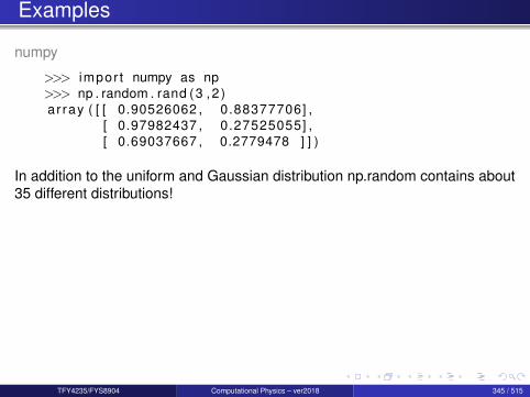
Examples
numpy
>>> impor t numpy as np>>> np . random . rand (3 ,2 )ar ray ( [ [ 0.90526062 , 0.88377706] ,
[ 0.97982437 , 0.27525055] ,[ 0.69037667 , 0.2779478 ] ] )
In addition to the uniform and Gaussian distribution np.random contains about35 different distributions!
TFY4235/FYS8904 Computational Physics – ver2018 345 / 515
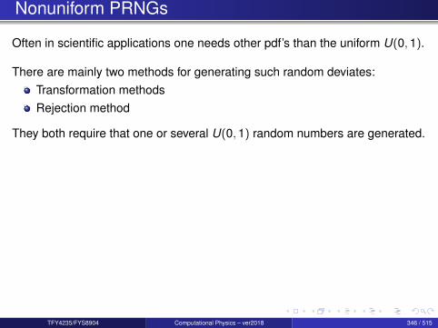
Nonuniform PRNGs
Often in scientific applications one needs other pdf’s than the uniform U(0,1).
There are mainly two methods for generating such random deviates:Transformation methodsRejection method
They both require that one or several U(0,1) random numbers are generated.
TFY4235/FYS8904 Computational Physics – ver2018 346 / 515
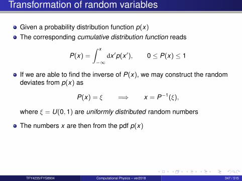
Transformation of random variables
Given a probability distribution function p(x)
The corresponding cumulative distribution function reads
P(x) =
∫ x
−∞dx ′p(x ′), 0 ≤ P(x) ≤ 1
If we are able to find the inverse of P(x), we may construct the randomdeviates from p(x) as
P(x) = ξ =⇒ x = P−1(ξ),
where ξ = U(0,1) are uniformly distributed random numbers
The numbers x are then from the pdf p(x)
TFY4235/FYS8904 Computational Physics – ver2018 347 / 515

Transformation of random variables
Algorithm1 Generate ξ = U(0,1)
2 Calculate x = P−1(ξ), which is distributed according to p(x)
This hinges on having an explicit expression for P−1(·).This is is not always possible!
TFY4235/FYS8904 Computational Physics – ver2018 348 / 515

Exponential deviates
p(x) = e−x 0 < x <∞P(x) = 1− e−x
Transformation (with ξ = ξ′ = U(0,1))
P(x) = ξ =⇒ x = − ln(1− ξ) = − ln(ξ′)
Code: from Numerical Recipes in C# include <math . h>f l o a t expdev ( long ∗ idum )/ / Returns an e x p o n e n t i a l l y d i s t r i b u t e d , p o s i t i v e ,/ / random dev ia te o f u n i t mean , using/ / ran1 ( idum ) as the source o f uni form dev ia tes .
f l o a t ran1 ( long ∗ idum ) ;f l o a t dum;do
dum=ran1 ( idum ) ;while (dum == 0 .0 ) ;return −log (dum) ;
TFY4235/FYS8904 Computational Physics – ver2018 349 / 515
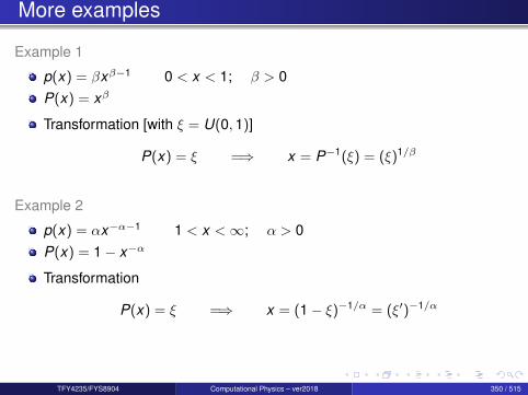
More examples
Example 1
p(x) = βxβ−1 0 < x < 1; β > 0P(x) = xβ
Transformation [with ξ = U(0,1)]
P(x) = ξ =⇒ x = P−1(ξ) = (ξ)1/β
Example 2
p(x) = αx−α−1 1 < x <∞; α > 0P(x) = 1− x−α
Transformation
P(x) = ξ =⇒ x = (1− ξ)−1/α = (ξ′)−1/α
TFY4235/FYS8904 Computational Physics – ver2018 350 / 515
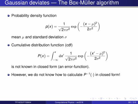
Gaussian deviates — The Box-Muller algorithm
Probability density function
p(x) =1√
2πσ2exp
(− (x − µ)2
2σ2
)mean µ and standard deviation σ
Cumulative distribution function (cdf)
P(x) =
∫ x
−∞dx ′
1√2πσ2
exp
(− (x ′ − µ)2
2σ2
)is not known in closed form (an error-function).
However, we do not know how to calculate P−1(·) in closed form!
TFY4235/FYS8904 Computational Physics – ver2018 351 / 515

Gaussian deviates —- The Box-Muller algorithm
The Box-Muller algorithmTrick : go from 1D to 2D and convert to polar coordinates (x1, x2)→ (r , φ)(we here for simplicity assume µ = 0 and σ = 1)
12π
exp
(−x2
1 + x22
2
)dx1 dx2 =
12π
exp
(− r2
2
)r dr dφ = pφ(φ)pr (r)drdφ
pφ(φ) =1
2πpr (r) = r exp
(− r2
2
)The cumulative distribution function for pr (r)
Pr (r) =
∫ r
0dr ′ r ′ exp
(− r ′2
2
)= 1− exp
(r2
2
)can be inverted to give [Pr (r) = ξ]
r =√−2 ln(1− ξ) =
√−2 ln ξ′
TFY4235/FYS8904 Computational Physics – ver2018 352 / 515

Gaussian deviates —- The Box-Muller algorithm
To generate two Gaussian random numbers we do
1 Generate ξ1 = U(0,1) and ξ2 = U(0,1) (uncorrelated)2 Calculate
x1 = r cos(φ) =√−2 ln ξ1 cos(2πξ2)
x2 = r sin(φ) =√−2 ln ξ1︸ ︷︷ ︸
r
sin(2πξ2)︸ ︷︷ ︸sin(φ)
3 The numbers x1 and x2 are uncorrelated Gaussian (or Normal) randomdeviates of mean 0 and standard deviation 1
Standard Gaussian random variables are typically denoted N(0,1)
Try this out for yourself! How can you make sure that the result is correct?
TFY4235/FYS8904 Computational Physics – ver2018 353 / 515

Rejection method
The rejection method (von Newmann 1947) is a general and powerfultechnique for generating random deviates from a distribution p(x).
In principle p(x) can be any pdf!
Assumptionsp(x) is computable (and is a pdf)p(x) ≤ f (x) for ∀x (f is a comparison function)F (x) =
∫ x−∞ dx ′f (x ′) exists and is invertable
Note : It is always possible to choose
f (x) = max p(x)
even if it may not be the best choice!
TFY4235/FYS8904 Computational Physics – ver2018 354 / 515

Rejection method
Algorithm1 Generate ξ1 = U(0,A), where A = F (∞)
2 Calculate x0 = F−1(ξ1)
3 Generate ξ2 = U(0, f (x0))
4 Number x0 should beaccepted if ξ2 ≤ p(x0)rejected if ξ2 > p(x0) (and start from point 1 again)
TFY4235/FYS8904 Computational Physics – ver2018 355 / 515
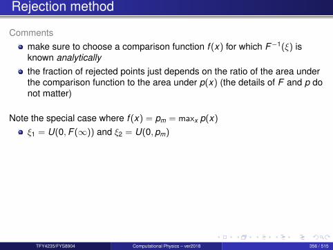
Rejection method
Commentsmake sure to choose a comparison function f (x) for which F−1(ξ) isknown analyticallythe fraction of rejected points just depends on the ratio of the area underthe comparison function to the area under p(x) (the details of F and p donot matter)
Note the special case where f (x) = pm = maxx p(x)
ξ1 = U(0,F (∞)) and ξ2 = U(0,pm)
TFY4235/FYS8904 Computational Physics – ver2018 356 / 515
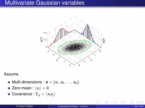
Multivariate Gaussian variables
Assume
Multi-dimensions : x = (x1, x2, . . . , xN)
Zero-mean : 〈xi〉 = 0Covariance : Σij =
⟨xixj⟩
TFY4235/FYS8904 Computational Physics – ver2018 357 / 515

Multivariate Gaussian variables
Define the covariance matrix
Σ =
Σ11 Σ12 Σ13 . . .Σ21 Σ22 Σ23 . . .Σ31 Σ32 Σ33 . . .
......
......
Then the multivariate Gaussian distribution reads
p(x) =1√
(2π)N |Σ|exp
(−1
2xT Σ−1x
),
In particular if Σ is diagonal it follows
p(x) =N∏
i=1
1√2πΣii
exp
(− x2
i2Σii
)i.e. , product of N uncorrelated 1D Gaussian distributions.
TFY4235/FYS8904 Computational Physics – ver2018 358 / 515

Multivariate Gaussian variables
In general the quadratic form xT Σ−1x is non-diagonal.However, it can be diagonalized by a linear transformation x = T y where T isan orthogonal (rotation) matrix; T T T = 1
xT Σ−1x = yT(
T T Σ−1T)
y
= yT Σ−1
y
=N∑
i=1
y2i
Σii
were we have defined
Σ = T T ΣT = T−1ΣT =(
T−1Σ−1T)−1
=(
T T Σ−1T)−1
Hence, Σ = T T ΣT is diagonal for a proper choice of T , and the diagonalelements are Σii = σ2
i .
TFY4235/FYS8904 Computational Physics – ver2018 359 / 515

Multivariate Gaussian variables
Algorithm: Generation of multivariate Gaussian variables1 Covariance matrix Σ is given2 Diagonalize Σ, that is, find its
eigenvalies σ2i N
i=1eignvector v iN
i=1;
3 Construct T = [v i ] with ‖v i‖ = 1 (main axis transformation)
4 Generate N independent (uncorrelated) Gaussian random variables yiwith variance σ2
i ; construct y
5 Make the transformation x = Ty
TFY4235/FYS8904 Computational Physics – ver2018 360 / 515

Section 10
Ordinary differential equations
TFY4235/FYS8904 Computational Physics – ver2018 361 / 515

Outline I
1 Introduction
2 Number representation and numerical precision
3 Finite differences and interpolation
4 Linear algebra
5 How to install libraries on a Linux system
6 Eigenvalue problems
7 Spectral methods
8 Numerical integration
TFY4235/FYS8904 Computational Physics – ver2018 362 / 515
Outline II9 Random numbers
10 Ordinary differential equations
11 Partial differential equations
12 Optimization
TFY4235/FYS8904 Computational Physics – ver2018 363 / 515
Ordinary differential equations (ODEs)General definition
Consider N ∈ N, an open subset U ⊂ RN+2, I ⊂ R, a function y : I 7→ R, andf ∈ C1(U,R). (I, y) is a solution of the differential equation
f (x , y , y ′, · · · , y (N)) = 0
if:y ∈ CN(I,R)
∀x ∈ I, (x , y(x), y ′(x), · · · , y (N)(x)) ∈ U∀x ∈ I, f (x , y(x), y ′(x), · · · , y (N)(x)) = 0
This is a N th order differential equation. We can further classify ODEs.linearnon-linearhomogeneous
To be made even more general
TFY4235/FYS8904 Computational Physics – ver2018 364 / 515
A short classification
An ODE is linear if f can be written as
f (x , y , y ′, · · · , y (N)) =N∑
i=0
λi y (i) + r
where (λi )i∈J0;1K and r are functions.A linear ODE is said homogeneous if r = 0.Examples:
Linear homogeneous Linear Non-linear
Free oscillator Forced oscillator Pendulum equation
y ′′ + ω2y = 0 y ′′ + ω2y = s y ′′ + ω2 sin y = 0
TFY4235/FYS8904 Computational Physics – ver2018 365 / 515
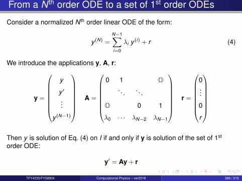
From a N th order ODE to a set of 1st order ODEs
Consider a normalized N th order linear ODE of the form:
y (N) =N−1∑i=0
λi y (i) + r (4)
We introduce the applications y, A, r:
y =
y
y ′
...
y (N−1)
A =
0 1 O
. . . . . .
O 0 1
λ0 · · · λN−2 λN−1
r =
0...
0
r
Then y is solution of Eq. (4) on I if and only if y is solution of the set of 1st
order ODE:
y′ = Ay + r
TFY4235/FYS8904 Computational Physics – ver2018 366 / 515
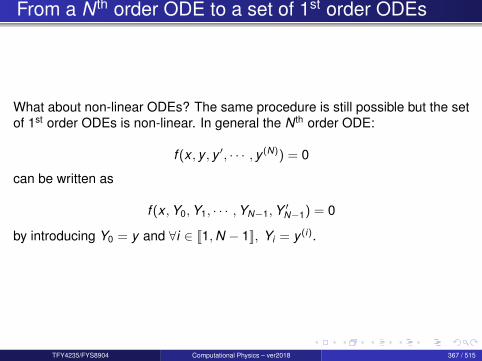
From a N th order ODE to a set of 1st order ODEs
What about non-linear ODEs? The same procedure is still possible but the setof 1st order ODEs is non-linear. In general the N th order ODE:
f (x , y , y ′, · · · , y (N)) = 0
can be written as
f (x ,Y0,Y1, · · · ,YN−1,Y ′N−1) = 0
by introducing Y0 = y and ∀i ∈ J1,N − 1K, Yi = y (i).
TFY4235/FYS8904 Computational Physics – ver2018 367 / 515
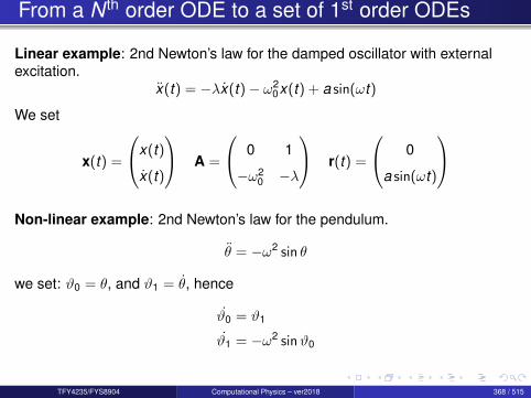
From a N th order ODE to a set of 1st order ODEs
Linear example: 2nd Newton’s law for the damped oscillator with externalexcitation.
x(t) = −λx(t)− ω20x(t) + a sin(ωt)
We set
x(t) =
x(t)
x(t)
A =
0 1
−ω20 −λ
r(t) =
0
a sin(ωt)
Non-linear example: 2nd Newton’s law for the pendulum.
θ = −ω2 sin θ
we set: ϑ0 = θ, and ϑ1 = θ, hence
ϑ0 = ϑ1
ϑ1 = −ω2 sinϑ0
TFY4235/FYS8904 Computational Physics – ver2018 368 / 515
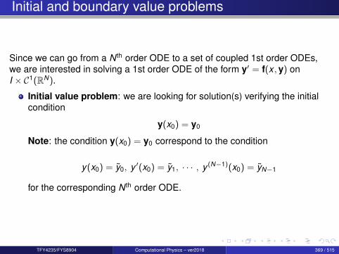
Initial and boundary value problems
Since we can go from a N th order ODE to a set of coupled 1st order ODEs,we are interested in solving a 1st order ODE of the form y′ = f(x ,y) onI × C1(RN).
Initial value problem: we are looking for solution(s) verifying the initialcondition
y(x0) = y0
Note: the condition y(x0) = y0 correspond to the condition
y(x0) = y0, y ′(x0) = y1, · · · , y (N−1)(x0) = yN−1
for the corresponding N th order ODE.
TFY4235/FYS8904 Computational Physics – ver2018 369 / 515
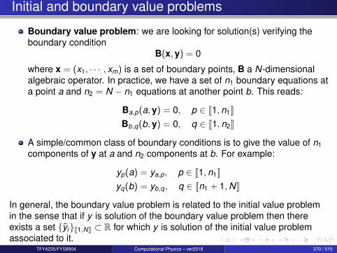
Initial and boundary value problems
Boundary value problem: we are looking for solution(s) verifying theboundary condition
B(x,y) = 0
where x = (x1, · · · , xm) is a set of boundary points, B a N-dimensionalalgebraic operator. In practice, we have a set of n1 boundary equations ata point a and n2 = N − n1 equations at another point b. This reads:
Ba,p(a,y) = 0, p ∈ J1,n1KBb,q(b,y) = 0, q ∈ J1,n2K
A simple/common class of boundary conditions is to give the value of n1components of y at a and n2 components at b. For example:
yp(a) = ya,p, p ∈ J1,n1Kyq(b) = yb,q , q ∈ Jn1 + 1,NK
In general, the boundary value problem is related to the initial value problemin the sense that if y is solution of the boundary value problem then thereexists a set yiJ1,NK ⊂ R for which y is solution of the initial value problemassociated to it.
TFY4235/FYS8904 Computational Physics – ver2018 370 / 515
Cauchy-Lipschitz Theorem
Consider the Cauchy problem
y ′ = f (x , y)
y(x0) = y0
If f is locally lipschitz continue with respect to the second variable, then aunique (maximal) solution exists to the Cauchy problem.
F : U → V is lipschitz continue if,
∃ k ≥ 0, ∀(x , y) ∈ U2, ‖F (x)− F (y)‖V ≤ k‖x − y‖U
TFY4235/FYS8904 Computational Physics – ver2018 371 / 515

How to solve numerically the Cauchy problem?
We consider now a Cauchy problem in 1D. The resolution of higher dimensionODE will use what follow for each equation of the set.
The key ideas to solve the Cauchy problem are:
Start from the initial point (x0, y0).Discretize the interval I on which the problem must be solve. This definesa step h. More advanced method can also involve adaptive step.Compute the next point (xn+1, yn+1) based on a scheme involving theprevious step (xn, yn) (single step methods) or a set a previous steps(multiple steps methods) and the corresponding evaluation of f at thoseprevious steps (or at intermediate steps).The scheme is often based on Taylor expansions and interpolationtechniques.
TFY4235/FYS8904 Computational Physics – ver2018 372 / 515

Single and multiple step methods
Some single step methods:
Euler’s methodsModified Euler’s methods (e.g. midpoint method)Runge-Kutta methods
Multiple steps methods:
Adams Bashforth methods (explicit)Adams Moulton methods (implicit)
TFY4235/FYS8904 Computational Physics – ver2018 373 / 515
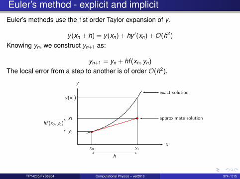
Euler’s method - explicit and implicitEuler’s methods use the 1st order Taylor expansion of y .
y(xn + h) = y(xn) + hy ′(xn) +O(h2)
Knowing yn, we construct yn+1 as:
yn+1 = yn + hf (xn, yn)
The local error from a step to another is of order O(h2).
x
y
x0 x1
y(x1)
y0
y1
exact solution
approximate solution
h
hf (x0, y0)
TFY4235/FYS8904 Computational Physics – ver2018 374 / 515
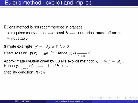
Euler’s method - explicit and implicit
Euler’s method is not recommended in practice.requires many steps =⇒ small h =⇒ numerical round off error.not stable
Simple example: y ′ = −λy with λ > 0
Exact solution: y(x) = y0e−λx . Hence y(x) −−−→x→∞
0
Approximate solution given by Euler’s explicit method: yn = y0(1− λh)n.Hence yn −−−→
n→∞0 ⇐⇒ |1− λh| < 1.
Stability condition: h < 2λ
TFY4235/FYS8904 Computational Physics – ver2018 375 / 515
Euler’s method - explicit and implicit
Stability can be improved by using an implicit scheme instead.
yn+1 = yn + hf (xn+1, yn+1)
Back to previous example:
yn+1 = yn − λh yn+1 ⇐⇒ yn+1 = yn1+λh
Hence the approximate solution reads:yn = y0
(1+λh)n −−−→n→∞
0 unconditionally.
Drawback: difficult to implement when f does not allow an explicit calculationof yn+1.
TFY4235/FYS8904 Computational Physics – ver2018 376 / 515
How to improve Euler’s method?
To improve Euler’s method one can:
Use a higher order Taylor expansion.Drawback: requires to evaluate partial derivatives of f . This method ishence not often use.Use intermediate points.Midpoint methodRunge-Kutta method
TFY4235/FYS8904 Computational Physics – ver2018 377 / 515
Midpoint method
Consider the midpoint between xn and xn+1: xn+1/2 = xn+xn+12 = xn + h
2Two Taylor expansions around the midpoint:
y(xn + h) = y(xn+1/2) +h2
y ′(xn+1/2) +h2
8y ′′(xn+1/2) +O(h3)
y(xn) = y(xn+1/2)− h2
y ′(xn+1/2) +h2
8y ′′(xn+1/2) +O(h3)
By substraction:
y(xn + h)− y(xn) = hy ′(xn+1/2) +O(h3)
Hence the midpoint method reads:1 Use Euler’s scheme with a step h/2 to construct yn+1/2.2 Compute the slope at that midpoint f (xn+1/2, yn+1/2).3 Use the midpoint slope to increment yn+1 from yn.
The local error made with the midpoint method is O(h3).
TFY4235/FYS8904 Computational Physics – ver2018 378 / 515

Midpoint method
x
y
x0 x1
y(x1)
y0
y1
x 12
exact solution
Euler solution
midpoint solution
h
hf (x 12, y 1
2)
In practice the algorithm reads:
k1 = hf (xn, yn)
k2 = hf (xn +h2, yn +
k1
2)
yn+1 = yn + k2
TFY4235/FYS8904 Computational Physics – ver2018 379 / 515
Runge-Kutta methods
Euler’s and the midpoint methods enters in a wider class a methods known asRunge-Kutta methods. As in the midpoint rule, the idea of higher orderRunge-Kutta methods is to cancel the error terms order by order. A largelyused method is the 4th-order Runge-Kutta method. The algorithm reads:
k1 = hf (xn, yn)
k2 = hf (xn +h2, yn +
k1
2)
k3 = hf (xn +h2, yn +
k2
2)
k4 = hf (xn + h, yn + k3)
yn+1 = yn +k1
6+
k2
3+
k3
3+
k4
6
The local error is O(h5), but the cost is 4 evaluations of f per step.
TFY4235/FYS8904 Computational Physics – ver2018 380 / 515

Multiple step methods
We have seen that steps close to the initial point are usually the most trustful,since errors add up from step to step. The key idea of multiple steps methodsis to use several previous step to compute the next one.
TFY4235/FYS8904 Computational Physics – ver2018 381 / 515
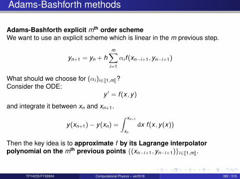
Adams-Bashforth methods
Adams-Bashforth explicit mth order schemeWe want to use an explicit scheme which is linear in the m previous step.
yn+1 = yn + hm∑
i=1
αi f (xn−i+1, yn−i+1)
What should we choose for (αi )i∈J1,mK?Consider the ODE:
y ′ = f (x , y)
and integrate it between xn and xn+1.
y(xn+1)− y(xn) =
∫ xn+1
xn
dx f (x , y(x))
Then the key idea is to approximate f by its Lagrange interpolatorpolynomial on the mth previous points (xn−i+1, yn−i+1)i∈J1,mK.
TFY4235/FYS8904 Computational Physics – ver2018 382 / 515
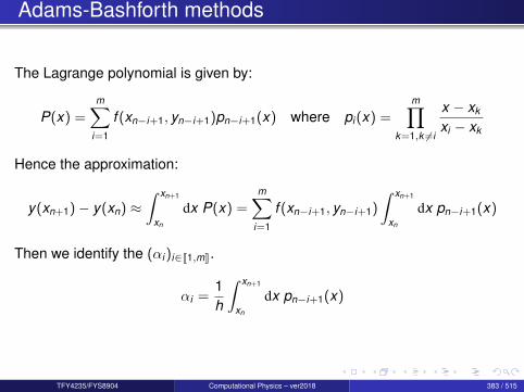
Adams-Bashforth methods
The Lagrange polynomial is given by:
P(x) =m∑
i=1
f (xn−i+1, yn−i+1)pn−i+1(x) where pi (x) =m∏
k=1,k 6=i
x − xk
xi − xk
Hence the approximation:
y(xn+1)− y(xn) ≈∫ xn+1
xn
dx P(x) =m∑
i=1
f (xn−i+1, yn−i+1)
∫ xn+1
xn
dx pn−i+1(x)
Then we identify the (αi )i∈J1,mK.
αi =1h
∫ xn+1
xn
dx pn−i+1(x)
TFY4235/FYS8904 Computational Physics – ver2018 383 / 515

Adams-Bashforth methods
Note:The integral in αi can be computed analytically (polynomial integrand).For a given order m, αi is independent of h. The coefficients can becomputed once and for all.The f (xn−i+1, yn−i+1)i∈J1,mK should be stored.The local error is O(hm)
This method is the equivalent of Newton-Cotes quadrature seenpreviously in the course.
m β α1/β α2/β α3/β α4/β
1 1 1
2 1/2 3 -1
3 1/12 23 -16 5
4 1/24 55 -59 37 -9
TFY4235/FYS8904 Computational Physics – ver2018 384 / 515

Adams-Moulton methods
Adams-Moulton implicit m + 1th order schemeWe want to use a scheme which is linear in the m previous step andf (xn+1, yn+1).
yn+1 = yn + hm∑
i=0
αi f (xn−i+1, yn−i+1)
The derivation of the (αi )i∈J1,mK is similar to the explicit method.
m β α0/β α1/β α2/β α3/β
0 1 1
1 1/2 1 1
2 1/12 5 8 -1
3 1/24 9 19 -5 1
TFY4235/FYS8904 Computational Physics – ver2018 385 / 515
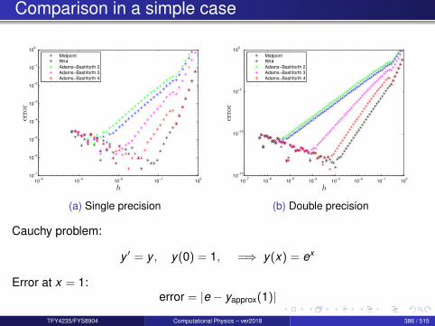
Comparison in a simple case
10−4
10−3
10−2
10−1
100
10−7
10−6
10−5
10−4
10−3
10−2
10−1
100
h
error
Midpoint
RK4
Adams−Bashforth 2
Adams−Bashforth 3
Adams−Bashforth 4
(a) Single precision
10−7
10−6
10−5
10−4
10−3
10−2
10−1
100
10−15
10−10
10−5
100
h
error
Midpoint
RK4
Adams−Bashforth 2
Adams−Bashforth 3
Adams−Bashforth 4
(b) Double precision
Cauchy problem:
y ′ = y , y(0) = 1, =⇒ y(x) = ex
Error at x = 1:error = |e − yapprox(1)|
TFY4235/FYS8904 Computational Physics – ver2018 386 / 515
Predictor-corrector
The key idea is PEC - Predict Estimate Correct:Predict yn+1 by using an explicit scheme.Estimate f (xn+1, yn+1) using the predicted value of yn+1.Correct yn+1 by using f (xn+1, yn+1) in an implicit scheme.
We can also estimate and correct several times within the same step until a acertain accuracy is reached. These methods are then often denoted P(EC)k Eif a fixed number of iteration is chosen or P(EC)∞E if a convergence conditionis used. The later is preferred for stiff ODEs, in order to benefit thestabilization of the implicit scheme.
TFY4235/FYS8904 Computational Physics – ver2018 387 / 515

Predictor-corrector
Example: 3rd order Adams-Bashforth-Moulton predictor-corrector method.Assume we have computed yn, yn−1, yn−2.
Prediction: Adams-Bashforth scheme
yPn+1 = yn +
h12
[23 f (xn, yn)− 16 f (xn−1, yn−1) + 5 f (xn−2, yn−2)]
Estimate f Pn+1 = f (xn+1, yP
n+1) and correction: Adams-Moulton scheme
yCn+1 = yn +
h12
[5 f P
n+1 + 8 f (xn, yn)− 1 f (xn−1, yn−1)]
Repeat EC using the new yCn+1 until |yk+1
n+1 − ykn+1| < ε
Terminate with an estimate of f (xn+1, y lastn+1).
TFY4235/FYS8904 Computational Physics – ver2018 388 / 515
Adaptive step methods
Principle: adapt locally the step to reach a set precision.To come
TFY4235/FYS8904 Computational Physics – ver2018 389 / 515
Two point boundary problem - Shooting method
We know now how to solve the Cauchy problem.Can we use the same techniques to solve a boundary problem?
Yes, this is the key idea of the shooting method!
A two point boundary problem can be seen as an initial value problem.The condition y(a) = ya and y(b) = yb relates to the condition y(a) = yaand y ′(a) = ya.Problem: how to find ya?
Consider the two problems
y ′′ = f (x , y , y ′), y(a) = ya, y(b) = yb (BVP)y ′′ = f (x , y , y ′), y(a) = ya, y ′(a) = ya (IVP)
We will denote y(.|ya) a solution of the IVP. Consider the differenceF (ya) = y(b|ya)− yb. Then the two problems are equivalent on the roots of F .
TFY4235/FYS8904 Computational Physics – ver2018 390 / 515
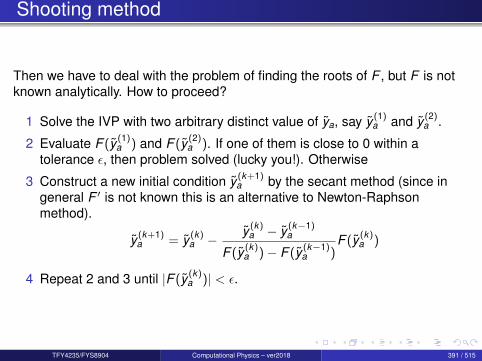
Shooting method
Then we have to deal with the problem of finding the roots of F , but F is notknown analytically. How to proceed?
1 Solve the IVP with two arbitrary distinct value of ya, say y (1)a and y (2)
a .
2 Evaluate F (y (1)a ) and F (y (2)
a ). If one of them is close to 0 within atolerance ε, then problem solved (lucky you!). Otherwise
3 Construct a new initial condition y (k+1)a by the secant method (since in
general F ′ is not known this is an alternative to Newton-Raphsonmethod).
y (k+1)a = y (k)
a − y (k)a − y (k−1)
a
F (y (k)a )− F (y (k−1)
a )F (y (k)
a )
4 Repeat 2 and 3 until |F (y (k)a )| < ε.
TFY4235/FYS8904 Computational Physics – ver2018 391 / 515

Shooting method
x
y y
a b
ya
yb
y(b|y (k−1)a )
y(b|y (k)a )
TFY4235/FYS8904 Computational Physics – ver2018 392 / 515
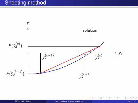
Shooting method
ya
F
y(k−1)a y
(k)a
F (y(k−1)a )
F (y(k)a )
y(k+1)a
solution
TFY4235/FYS8904 Computational Physics – ver2018 393 / 515
Shooting method
Note:You can show as an exercise that in the linear case, the solution is givenby one iteration.In the non-linear case, neither the existence or the unicity of a solution isa priori guaranty in general.
TFY4235/FYS8904 Computational Physics – ver2018 394 / 515
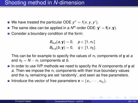
Shooting method in N-dimension
We have treated the particular ODE y ′′ = f (x , y , y ′).The same idea can be applied in a N th-order ODE: y′ = f(x ,y).Consider a boundary condition of the form:
Ba,p(a,y) = 0, p ∈ J1,n1KBb,q(b,y) = 0, q ∈ J1,n2K.
This can be for example to specify the values of n1 components of y at aand n2 = N − n1 components at b.In order to use IVP methods we need to specify the N components of y ata. Then we impose the n1 components with their true boundary valuesand the n2 remaining are set ’randomly’, and seen as free parameters.Introduce the vector of free parameters v = (v1, · · · , vn2 ).
TFY4235/FYS8904 Computational Physics – ver2018 395 / 515

Shooting method in N-dimension
The initial point y(a) is then given by:
y(a) = y(a,v)
where y already contains the n1 true boundary values at a.Then given this initial condition, we can use IVP methods to solve thisparticular Cauchy problem and determine y(b|v).Using the boundary functional Bb,i , i ∈ J1,n2K, we can construct adiscrepancy vector F such that:
Fi (v) = Bb,i (b,y(b|v))
We must then use an iteration scheme to find v that cancels F.ND Newton-Raphson scheme
vk+1 = vk + δv, J δv = −F
Jij =∂Fi
∂vj≈ Fi (v1, · · · , vj + ∆vj , · · · , vn2 )− Fi (v1, · · · , vn2 )
∆vj
TFY4235/FYS8904 Computational Physics – ver2018 396 / 515
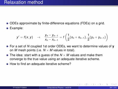
Relaxation method
ODEs approximate by finite-difference equations (FDEs) on a grid.Example:
y ′ = f (x , y) → yn − yn−1
xn − xn−1= f
(12
(xn + xn−1),12
(yn + yn−1)
)For a set of N coupled 1st order ODEs, we want to determine values of yon M mesh points (i.e. N ×M values in total).The idea: start with a guess of the N ×M values and make themconverge to the true value using an adequate iterative scheme.How to find an adequate iterative scheme?
TFY4235/FYS8904 Computational Physics – ver2018 397 / 515
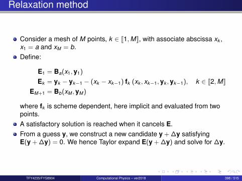
Relaxation method
Consider a mesh of M points, k ∈ J1,MK, with associate abscissa xk ,x1 = a and xM = b.Define:
E1 = Ba(x1,y1)
Ek = yk − yk−1 − (xk − xk−1) fk (xk , xk−1,yk ,yk−1), k ∈ J2,MKEM+1 = Bb(xM ,yM)
where fk is scheme dependent, here implicit and evaluated from twopoints.A satisfactory solution is reached when it cancels E.From a guess y, we construct a new candidate y + ∆y satisfyingE(y + ∆y) = 0. We hence Taylor expand E(y + ∆y) and solve for ∆y.
TFY4235/FYS8904 Computational Physics – ver2018 398 / 515
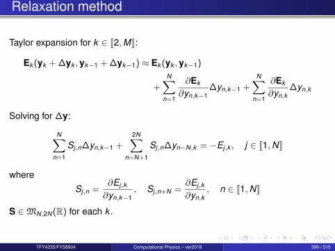
Relaxation method
Taylor expansion for k ∈ J2,MK:
Ek (yk + ∆yk ,yk−1 + ∆yk−1) ≈ Ek (yk ,yk−1)
+N∑
n=1
∂Ek
∂yn,k−1∆yn,k−1 +
N∑n=1
∂Ek
∂yn,k∆yn,k
Solving for ∆y:
N∑n=1
Sj,n∆yn,k−1 +2N∑
n=N+1
Sj,n∆yn−N,k = −Ej,k , j ∈ J1,NK
whereSj,n =
∂Ej,k
∂yn,k−1, Sj,n+N =
∂Ej,k
∂yn,k, n ∈ J1,NK
S ∈MN,2N(R) for each k .
TFY4235/FYS8904 Computational Physics – ver2018 399 / 515
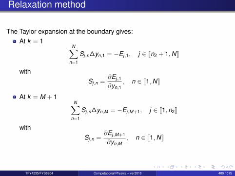
Relaxation method
The Taylor expansion at the boundary gives:At k = 1
N∑n=1
Sj,n∆yn,1 = −Ej,1, j ∈ Jn2 + 1,NK
withSj,n =
∂Ej,1
∂yn,1, n ∈ J1,NK
At k = M + 1N∑
n=1
Sj,n∆yn,M = −Ej,M+1, j ∈ J1,n2K
withSj,n =
∂Ej,M+1
∂yn,M, n ∈ J1,NK
TFY4235/FYS8904 Computational Physics – ver2018 400 / 515

Relaxation method
We have then a linear system to solve for ∆y.
TFY4235/FYS8904 Computational Physics – ver2018 401 / 515

Section 11
Partial differential equations
TFY4235/FYS8904 Computational Physics – ver2018 402 / 515
Outline I
1 Introduction
2 Number representation and numerical precision
3 Finite differences and interpolation
4 Linear algebra
5 How to install libraries on a Linux system
6 Eigenvalue problems
7 Spectral methods
8 Numerical integration
TFY4235/FYS8904 Computational Physics – ver2018 403 / 515
Outline II9 Random numbers
10 Ordinary differential equations
11 Partial differential equationsParabolic PDEsHyperbolic PDEsElliptic PDEsOther methods
12 Optimization
TFY4235/FYS8904 Computational Physics – ver2018 404 / 515
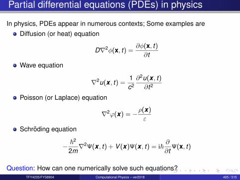
Partial differential equations (PDEs) in physics
In physics, PDEs appear in numerous contexts; Some examples areDiffusion (or heat) equation
D∇2φ(x, t) =∂φ(x, t)∂t
Wave equation
∇2u(x , t) =1c2∂2u(x , t)∂t2
Poisson (or Laplace) equation
∇2ϕ(x) = −ρ(x)
ε
Schroding equation
− ~2
2m∇2Ψ(x , t) + V (x)Ψ(x , t) = i~
∂
∂tΨ(x, t)
Question: How can one numerically solve such equations?TFY4235/FYS8904 Computational Physics – ver2018 405 / 515

Classification of PDEs
Consider the general 2nd order PDE
A(x , y)∂2u∂x2 + 2B(x , y)
∂2u∂x∂y
+ C(x , y)∂2u∂y2 = F (x , y ,u,
∂u∂x
,∂u∂y
)
PDEs are classified as:
ParabolicB2 − AC = 0Diffusion/heat equation : uxx = ut
HyperbolicB2 − AC > 0Wave equation : uxx − utt = 0
EllipticB2 − AC < 0Laplace’s equation : uxx + uyy = 0
www.math.utep.edu/studentresources/lecture_notes/pdf/math_5314.pdf
TFY4235/FYS8904 Computational Physics – ver2018 406 / 515
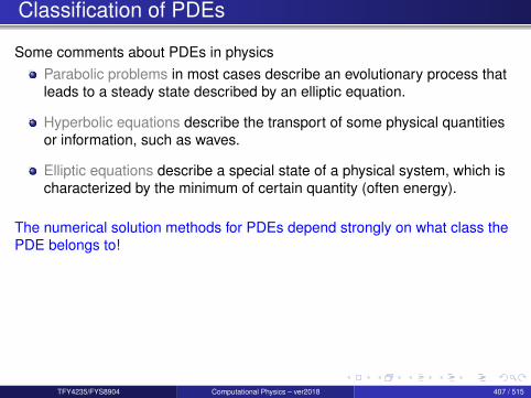
Classification of PDEs
Some comments about PDEs in physicsParabolic problems in most cases describe an evolutionary process thatleads to a steady state described by an elliptic equation.
Hyperbolic equations describe the transport of some physical quantitiesor information, such as waves.
Elliptic equations describe a special state of a physical system, which ischaracterized by the minimum of certain quantity (often energy).
The numerical solution methods for PDEs depend strongly on what class thePDE belongs to!
TFY4235/FYS8904 Computational Physics – ver2018 407 / 515

Parabolic PDEs
TFY4235/FYS8904 Computational Physics – ver2018 408 / 515
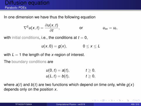
Diffusion equationParabolic PDEs
In one dimension we have thus the following equation
∇2u(x , t) =∂u(x , t)∂t
, or uxx = ut ,
with initial conditions, i.e., the conditions at t = 0,
u(x ,0) = g(x), 0 ≤ x ≤ L
with L = 1 the length of the x-region of interest.
The boundary conditions are
u(0, t) = a(t), t ≥ 0,u(L, t) = b(t), t ≥ 0,
where a(t) and b(t) are two functions which depend on time only, while g(x)depends only on the position x .
TFY4235/FYS8904 Computational Physics – ver2018 409 / 515
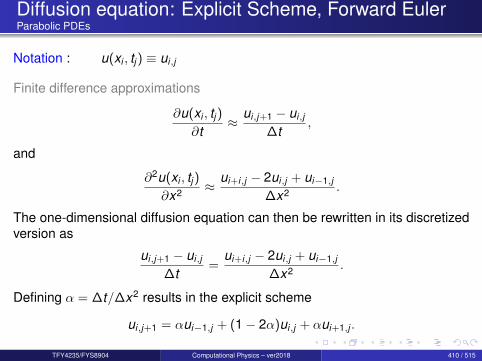
Diffusion equation: Explicit Scheme, Forward EulerParabolic PDEs
Notation : u(xi , tj ) ≡ ui,j
Finite difference approximations
∂u(xi , tj )∂t
≈ ui,j+1 − ui,j
∆t,
and
∂2u(xi , tj )∂x2 ≈ ui+i,j − 2ui,j + ui−1,j
∆x2 .
The one-dimensional diffusion equation can then be rewritten in its discretizedversion as
ui,j+1 − ui,j
∆t=
ui+i,j − 2ui,j + ui−1,j
∆x2 .
Defining α = ∆t/∆x2 results in the explicit scheme
ui,j+1 = αui−1,j + (1− 2α)ui,j + αui+1,j .
TFY4235/FYS8904 Computational Physics – ver2018 410 / 515
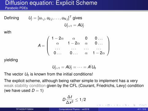
Diffusion equation: Explicit SchemeParabolic PDEs
Defining Uj = [u1,j ,u2,j , . . . ,uN,j ]T gives
Uj+1 = AUj
with
A =
1− 2α α 0 0 . . .α 1− 2α α 0 . . .. . . . . . . . . . . .
0 . . . 0 . . . α 1− 2α
yielding
Uj+1 = AUj = · · · = AjU0
The vector U0 is known from the initial conditions!
The explicit scheme, although being rather simple to implement has a veryweak stability condition given by the CFL (Courant, Friedrichs, Levy) condition(we have used D = 1)
D∆t
∆x2 ≤ 1/2
TFY4235/FYS8904 Computational Physics – ver2018 411 / 515
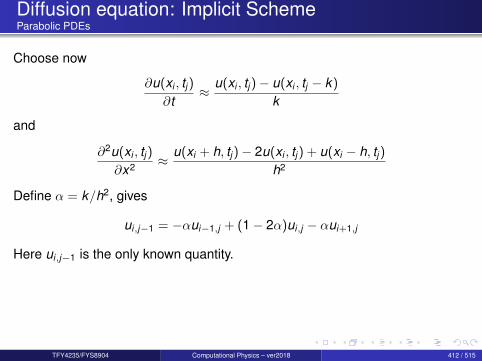
Diffusion equation: Implicit SchemeParabolic PDEs
Choose now
∂u(xi , tj )∂t
≈ u(xi , tj )− u(xi , tj − k)
k
and
∂2u(xi , tj )∂x2 ≈ u(xi + h, tj )− 2u(xi , tj ) + u(xi − h, tj )
h2
Define α = k/h2, gives
ui,j−1 = −αui−1,j + (1− 2α)ui,j − αui+1,j
Here ui,j−1 is the only known quantity.
TFY4235/FYS8904 Computational Physics – ver2018 412 / 515
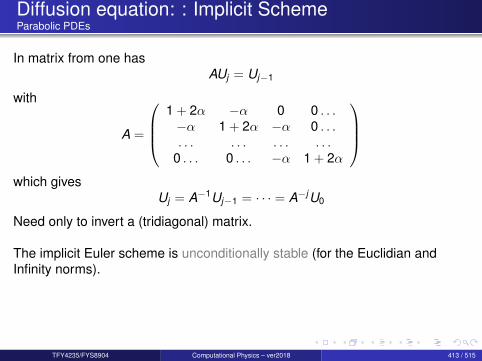
Diffusion equation: : Implicit SchemeParabolic PDEs
In matrix from one hasAUj = Uj−1
with
A =
1 + 2α −α 0 0 . . .−α 1 + 2α −α 0 . . .. . . . . . . . . . . .
0 . . . 0 . . . −α 1 + 2α
which gives
Uj = A−1Uj−1 = · · · = A−jU0
Need only to invert a (tridiagonal) matrix.
The implicit Euler scheme is unconditionally stable (for the Euclidian andInfinity norms).
TFY4235/FYS8904 Computational Physics – ver2018 413 / 515

Diffusion equation: Brute Force Implicit Scheme,inefficient algorithmParabolic PDEs
Some Fortran code:
! now invert the matrixCALL matinv( a, ndim, det)DO i = 1, m
DO l=1, ndimu(l) = DOT_PRODUCT(a(l,:),v(:))
ENDDOv = ut = i*kDO j=1, ndim
WRITE(6,*) t, j*h, v(j)ENDDO
ENDDO
Question: Why is this algorithm inefficient?
TFY4235/FYS8904 Computational Physics – ver2018 414 / 515
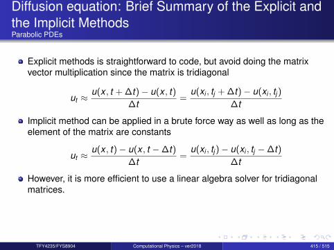
Diffusion equation: Brief Summary of the Explicit andthe Implicit MethodsParabolic PDEs
Explicit methods is straightforward to code, but avoid doing the matrixvector multiplication since the matrix is tridiagonal
ut ≈u(x , t + ∆t)− u(x , t)
∆t=
u(xi , tj + ∆t)− u(xi , tj )∆t
Implicit method can be applied in a brute force way as well as long as theelement of the matrix are constants
ut ≈u(x , t)− u(x , t −∆t)
∆t=
u(xi , tj )− u(xi , tj −∆t)∆t
However, it is more efficient to use a linear algebra solver for tridiagonalmatrices.
TFY4235/FYS8904 Computational Physics – ver2018 415 / 515
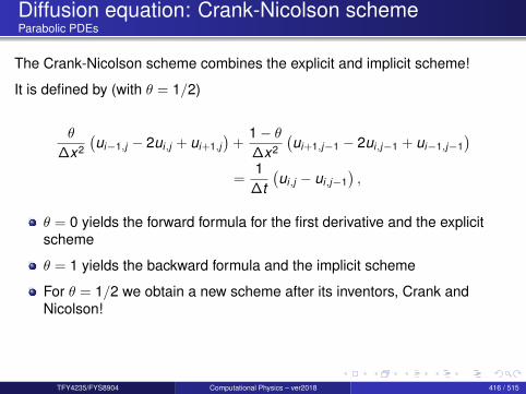
Diffusion equation: Crank-Nicolson schemeParabolic PDEs
The Crank-Nicolson scheme combines the explicit and implicit scheme!
It is defined by (with θ = 1/2)
θ
∆x2
(ui−1,j − 2ui,j + ui+1,j
)+
1− θ∆x2
(ui+1,j−1 − 2ui,j−1 + ui−1,j−1
)=
1∆t(ui,j − ui,j−1
),
θ = 0 yields the forward formula for the first derivative and the explicitscheme
θ = 1 yields the backward formula and the implicit scheme
For θ = 1/2 we obtain a new scheme after its inventors, Crank andNicolson!
TFY4235/FYS8904 Computational Physics – ver2018 416 / 515

Diffusion equation: Crank-Nicolson schemeParabolic PDEs
Using our previous definition of α = ∆t/∆x2 we can rewrite the latter equationas
−αui−1,j + (2 + 2α) ui,j − αui+1,j = αui−1,j−1 + (2− 2α) ui,j−1 + αui+1,j−1,
or in matrix-vector form as
(2I + αB) Uj = (2I − αB) Uj−1,
where the vector Uj is the same as defined in the implicit case while thematrix B is
B =
2 −1 0 0 . . .−1 2 −1 0 . . .. . . . . . . . . . . .
0 . . . 0 . . . 2
TFY4235/FYS8904 Computational Physics – ver2018 417 / 515
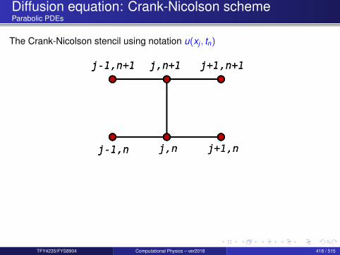
Diffusion equation: Crank-Nicolson schemeParabolic PDEs
The Crank-Nicolson stencil using notation u(xj , tn)
TFY4235/FYS8904 Computational Physics – ver2018 418 / 515

Diffusion equation: AnalysisParabolic PDEs
We now want to take a look at stability and accuracy!
Some relevant questions areHow accurate is a discretization scheme?Is it stable for some or any choice of ∆x and ∆t?How can this information be obtained (if relevant)?etc
Accuracy is studied by Taylor expanding the scheme around a common point!
TFY4235/FYS8904 Computational Physics – ver2018 419 / 515

Diffusion equation: AnalysisParabolic PDEs
We start with the forward Euler scheme and Taylor expand u(x , t + ∆t),u(x + ∆x , t) and u(x −∆x , t) about (x , t)
u(x + ∆x , t) = u(x , t) +∂u(x , t)∂x
∆x +∂2u(x , t)
2∂x2 ∆x2 +O(∆x3),
u(x −∆x , t) = u(x , t)− ∂u(x , t)∂x
∆x +∂2u(x , t)
2∂x2 ∆x2 +O(∆x3),
u(x , t + ∆t) = u(x , t) +∂u(x , t)∂t
∆t +O(∆t2).
With these Taylor expansions the approximations for the derivatives takes theform [
∂u(x , t)∂t
]approx
=∂u(x , t)∂t
+O(∆t),[∂2u(x , t)∂x2
]approx
=∂2u(x , t)∂x2 +O(∆x2).
It is easy to convince oneself that the backward Euler method must have thesame truncation errors as the forward Euler scheme.
TFY4235/FYS8904 Computational Physics – ver2018 420 / 515
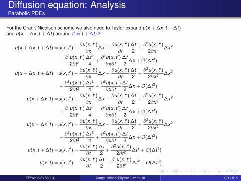
Diffusion equation: AnalysisParabolic PDEs
For the Crank-Nicolson scheme we also need to Taylor expand u(x + ∆x , t + ∆t)and u(x −∆x , t + ∆t) around t ′ = t + ∆t/2.
u(x + ∆x , t + ∆t) =u(x , t ′) +∂u(x , t ′)∂x
∆x +∂u(x , t ′)
∂t∆t2
+∂2u(x , t ′)
2∂x2 ∆x2
+∂2u(x , t ′)
2∂t2∆t2
4+∂2u(x , t ′)∂x∂t
∆t2
∆x +O(∆t3)
u(x −∆x , t + ∆t) =u(x , t ′)− ∂u(x , t ′)∂x
∆x +∂u(x , t ′)
∂t∆t2
+∂2u(x , t ′)
2∂x2 ∆x2
+∂2u(x , t ′)
2∂t2∆t2
4− ∂2u(x , t ′)
∂x∂t∆t2
∆x +O(∆t3)
u(x + ∆x , t) =u(x , t ′) +∂u(x , t ′)∂x
∆x − ∂u(x , t ′)∂t
∆t2
+∂2u(x , t ′)
2∂x2 ∆x2
+∂2u(x , t ′)
2∂t2∆t2
4− ∂2u(x , t ′)
∂x∂t∆t2
∆x +O(∆t3)
u(x −∆x , t) =u(x , t ′)− ∂u(x , t ′)∂x
∆x − ∂u(x , t ′)∂t
∆t2
+∂2u(x , t ′)
2∂x2 ∆x2
+∂2u(x , t ′)
2∂t2∆t2
4+∂2u(x , t ′)∂x∂t
∆t2
∆x +O(∆t3)
u(x , t + ∆t) =u(x , t ′) +∂u(x , t ′)
∂t∆t
2+∂2u(x , t ′)
2∂t2 ∆t2 +O(∆t3)
u(x , t) =u(x , t ′)− ∂u(x , t ′)∂t
∆t2
+∂2u(x , t ′)
2∂t2 ∆t2 +O(∆t3)
TFY4235/FYS8904 Computational Physics – ver2018 421 / 515
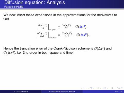
Diffusion equation: AnalysisParabolic PDEs
We now insert these expansions in the approximations for the derivatives tofind [
∂u(x,t′)∂t
]approx
= ∂u(x,t′)∂t +O(∆t2),[
∂2u(x,t′)∂x2
]approx
= ∂2u(x,t′)∂x2 +O(∆x2).
Hence the truncation error of the Crank-Nicolson scheme is O(∆t2) andO(∆x2), i.e. 2nd order in both space and time!
TFY4235/FYS8904 Computational Physics – ver2018 422 / 515

Diffusion equation: AnalysisParabolic PDEs
The following table summarizes the three methods.
Scheme: Truncation Error: Stability requirements:Crank-Nicolson O(∆x2) and O(∆t2) Stable for all ∆t and ∆x .Backward Euler O(∆x2) and O(∆t) Stable for all ∆t and ∆x .Forward Euler O(∆x2) and O(∆t) ∆t ≤ 1
2 ∆x2
Table: Comparison of the different schemes.
The stability criterion is derived by using the von Neumann stability criterion10
where the error is decomposed into Fourier series.
A finite difference scheme is stable if the errors made at one time step of thecalculation do not cause the errors to increase as the computations arecontinued.
10http://en.wikipedia.org/wiki/Von_Neumann_stability_analysisTFY4235/FYS8904 Computational Physics – ver2018 423 / 515
Diffusion equation: AnalysisParabolic PDEs
Illustration of the von Neumann stability criteria for the forward Euler scheme.
To be added.....!
In the mean time consult e.g. http://en.wikipedia.org/wiki/Von_Neumann_stability_analysis!
TFY4235/FYS8904 Computational Physics – ver2018 424 / 515

Diffusion equation: AnalysisParabolic PDEs
It cannot be repeated enough, it is always very useful to find cases where onecan compare the numerics and the developed algorithms and codes withanalytic solution.
The above case is also particularly simple. We have the following partialdifferential equation
∇2u(x , t) =∂u(x , t)∂t
,
with initial conditions
u(x ,0) = g(x) 0 < x < L.
The boundary conditions are
u(0, t) = 0 t ≥ 0, u(L, t) = 0 t ≥ 0,
TFY4235/FYS8904 Computational Physics – ver2018 425 / 515

Diffusion equation: AnalysisParabolic PDEs
We assume that we have solutions of the form (separation of variable)
u(x , t) = F (x)G(t),
which inserted in the partial differential equation results in
F ′′
F=
G′
G,
where the derivative is with respect to x on the left hand side and with respectto t on right hand side. This equation should hold for all x and t . We mustrequire the rhs and lhs to be equal to a constant.
We call this constant −λ2. This gives us the two differential equations,
F ′′ + λ2F = 0; G′ = −λ2G,
with general solutions
F (x) = A sin(λx) + B cos(λx); G(t) = Ce−λ2t .
TFY4235/FYS8904 Computational Physics – ver2018 426 / 515

Diffusion equation: AnalysisParabolic PDEs
To satisfy the boundary conditions we require B = 0 and λ = nπ/L. Onesolution is therefore found to be
u(x , t) = An sin(nπx/L)e−n2π2t/L2.
But there are infinitely many possible n values (infinite number of solutions).
Moreover, the diffusion equation is linear and because of this we know that asuperposition of solutions will also be a solution of the equation.
We may therefore write
u(x , t) =∞∑
n=1
An sin(nπx/L)e−n2π2t/L2.
TFY4235/FYS8904 Computational Physics – ver2018 427 / 515

Diffusion equation: AnalysisParabolic PDEs
The coefficient An is in turn determined from the initial condition. We require
u(x ,0) = g(x) =∞∑
n=1
An sin(nπx/L).
The coefficient An is the Fourier coefficients for the function g(x). Because ofthis, An is given by (from the theory on Fourier series)
An =2L
∫ L
0dx g(x) sin(nπx/L)
Different g(x) functions will obviously result in different results for An.
TFY4235/FYS8904 Computational Physics – ver2018 428 / 515

Diffusion equation: Some examplesParabolic PDEs
Numerical examples:
Let look at the following diffusion equation
∂tC(x , t) = ∂x [D(x)∂xC(x , t)]
C(x ,0) = C0 δ (x)
where now the diffusion constant, D(x), is position dependent (and C0 someconstant).
So how should the discretization scheme for this PDE be?In particular, how should the spatial derivatives be discretized?
TFY4235/FYS8904 Computational Physics – ver2018 429 / 515
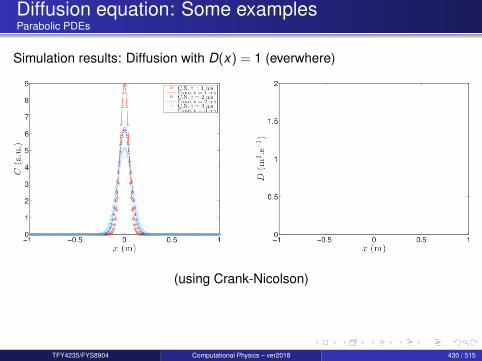
Diffusion equation: Some examplesParabolic PDEs
Simulation results: Diffusion with D(x) = 1 (everwhere)
(using Crank-Nicolson)
TFY4235/FYS8904 Computational Physics – ver2018 430 / 515

Diffusion equation: Some examplesParabolic PDEs
Simulation results: Diffusion with piecewise constant D(x)
Exercise: Reproduce these results!
TFY4235/FYS8904 Computational Physics – ver2018 431 / 515
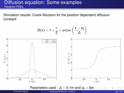
Diffusion equation: Some examplesParabolic PDEs
Simulation results: Crank-Nicolson for the position dependent diffusionconstant
D(x) = 1 +π
2+ arctan
(x − x0
∆
)
Parameters used : ∆ = 0.1m and x0 = 0mTFY4235/FYS8904 Computational Physics – ver2018 432 / 515
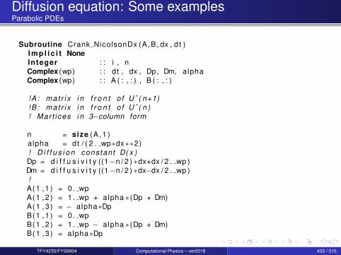
Diffusion equation: Some examplesParabolic PDEs
Subroutine Crank NicolsonDx (A,B, dx , d t )I m p l i c i t NoneInteger : : i , nComplex (wp) : : dt , dx , Dp, Dm, alphaComplex (wp) : : A ( : , : ) , B ( : , : )
!A : mat r i x i n f r o n t o f Uˆ ( n+1)!B : mat r i x i n f r o n t o f Uˆ ( n )! Mar t ices i n 3−column form
n = size (A, 1 )alpha = dt / ( 2 . wp∗dx∗∗2)! D i f f u s i o n constant D( x )Dp = d i f f u s i v i t y ((1−n / 2 ) ∗dx+dx / 2 . wp )Dm = d i f f u s i v i t y ((1−n / 2 ) ∗dx−dx / 2 . wp )!A(1 ,1 ) = 0 . wpA(1 ,2 ) = 1 . wp + alpha ∗ (Dp + Dm)A(1 ,3 ) = − alpha∗DpB(1 ,1 ) = 0 . wpB(1 ,2 ) = 1 . wp − alpha ∗ (Dp + Dm)B(1 ,3 ) = alpha∗Dp
TFY4235/FYS8904 Computational Physics – ver2018 433 / 515
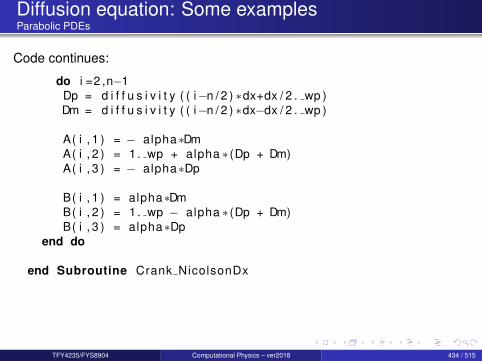
Diffusion equation: Some examplesParabolic PDEs
Code continues:
do i =2 ,n−1Dp = d i f f u s i v i t y ( ( i−n / 2 ) ∗dx+dx / 2 . wp )Dm = d i f f u s i v i t y ( ( i−n / 2 ) ∗dx−dx / 2 . wp )
A( i , 1 ) = − alpha∗DmA( i , 2 ) = 1 . wp + alpha ∗ (Dp + Dm)A( i , 3 ) = − alpha∗Dp
B( i , 1 ) = alpha∗DmB( i , 2 ) = 1 . wp − alpha ∗ (Dp + Dm)B( i , 3 ) = alpha∗Dp
end do
end Subroutine Crank NicolsonDx
TFY4235/FYS8904 Computational Physics – ver2018 434 / 515

Hyperbolic PDEs
TFY4235/FYS8904 Computational Physics – ver2018 435 / 515
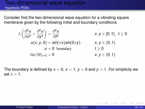
Two-dimensional wave equationHyperbolic PDEs
Consider first the two-dimensional wave equation for a vibrating squaremembrane given by the following initial and boundary conditions
λ
(∂2u∂x2 +
∂2u∂y2
)=∂2u∂t2 x , y ∈ [0,1], t ≥ 0
u(x , y ,0) = sin(πx)sin(2πy) x , y ∈ (0,1)
u = 0 boundary t ≥ 0∂u/∂t |t=0 = 0 x , y ∈ (0,1)
The boundary is defined by x = 0, x = 1, y = 0 and y = 1. For simplicity weset λ = 1.
TFY4235/FYS8904 Computational Physics – ver2018 436 / 515
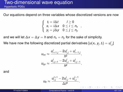
Two-dimensional wave equationHyperbolic PDEs
Our equations depend on three variables whose discretized versions are now tl = l∆t l ≥ 0xi = i∆x 0 ≤ i ≤ nxyj = j∆y 0 ≤ j ≤ ny
,
and we will let ∆x = ∆y = h and nx = ny for the sake of simplicity.
We have now the following discretized partial derivatives [u(xi , yj , tl ) = uli,j ]
uxx ≈ul
i+1,j − 2uli,j + ul
i−1,j
h2 ,
uyy ≈ul
i,j+1 − 2uli,j + ul
i,j−1
h2 ,
and
utt ≈ul+1
i,j − 2uli,j + ul−1
i,j
∆t2 .
TFY4235/FYS8904 Computational Physics – ver2018 437 / 515

Two-dimensional wave equationHyperbolic PDEs
We merge this into the discretized 2 + 1-dimensional wave equation as
ul+1i,j = 2ul
i,j − ul−1i,j +
∆t2
h2
(ul
i+1,j − 4uli,j + ul
i−1,j + uli,j+1 + ul
i,j−1
),
where again we have an explicit scheme with ul+1i,j as the only unknown
quantity. It is easy to account for different step lengths for x and y . The partialderivative is treated in much the same way as for the one-dimensional case,except that we now have an additional index due to the extra spatialdimension, viz., we need to compute u−1
i,j through
u−1i,j = u0
i,j +∆t2h2
(u0
i+1,j − 4u0i,j + u0
i−1,j + u0i,j+1 + u0
i,j−1),
in our setup of the initial conditions.
TFY4235/FYS8904 Computational Physics – ver2018 438 / 515

Two-dimensional wave equation: Code exampleHyperbolic PDEs
We show here how to implement the two-dimensional wave equation
/ / A f t e r i n i t i a l i z a t i o n s and d e c l a r a t i o n o f va r i a b l e sfor ( i n t i = 0 ; i < n ; i ++ )
u [ i ] = new double [ n ] ;uLast [ i ] = new double [ n ] ;uNext [ i ] = new double [ n ] ;x [ i ] = i ∗h ;y [ i ] = x [ i ] ;
/ / i n i t i a l i z i n gfor ( i n t i = 0 ; i < n ; i ++ ) / / s e t t i n g i n i t i a l step
for ( i n t j = 0 ; j < n ; j ++ ) uLast [ i ] [ j ] = sin ( PI∗x [ i ] ) ∗sin (2∗PI∗y [ j ] ) ;
TFY4235/FYS8904 Computational Physics – ver2018 439 / 515
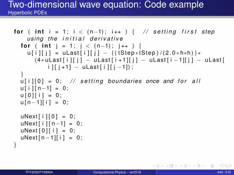
Two-dimensional wave equation: Code exampleHyperbolic PDEs
for ( i n t i = 1 ; i < ( n−1) ; i ++ ) / / s e t t i n g f i r s t stepusing the i n i t i a l d e r i v a t i v e
for ( i n t j = 1 ; j < ( n−1) ; j ++ ) u [ i ] [ j ] = uLast [ i ] [ j ] − ( ( tStep∗ tStep ) / ( 2 . 0 ∗ h∗h ) ) ∗
(4∗ uLast [ i ] [ j ] − uLast [ i + 1 ] [ j ] − uLast [ i −1][ j ] − uLast [i ] [ j +1] − uLast [ i ] [ j −1]) ;
u [ i ] [ 0 ] = 0 ; / / s e t t i n g boundaries once and f o r a l lu [ i ] [ n−1] = 0 ;u [ 0 ] [ i ] = 0 ;u [ n−1][ i ] = 0 ;
uNext [ i ] [ 0 ] = 0 ;uNext [ i ] [ n−1] = 0 ;uNext [ 0 ] [ i ] = 0 ;uNext [ n−1][ i ] = 0 ;
TFY4235/FYS8904 Computational Physics – ver2018 440 / 515

Two-dimensional wave equation: Code exampleHyperbolic PDEs
/ / i t e r a t i n g i n t imedouble t = 0.0 + tStep ;i n t i t e r = 0 ;
while ( t < t F i n a l ) i t e r ++;t = t + tStep ;
for ( i n t i = 1 ; i < ( n−1) ; i ++ ) / / computing next stepfor ( i n t j = 1 ; j < ( n−1) ; j ++ )
uNext [ i ] [ j ] = 2∗u [ i ] [ j ] − uLast [ i ] [ j ] − ( ( tStep∗ tStep )/ ( h∗h ) ) ∗
(4∗u [ i ] [ j ] − u [ i + 1 ] [ j ] − u [ i −1][ j ] − u [ i ] [ j +1] − u [ i] [ j −1]) ;
TFY4235/FYS8904 Computational Physics – ver2018 441 / 515
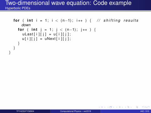
Two-dimensional wave equation: Code exampleHyperbolic PDEs
for ( i n t i = 1 ; i < ( n−1) ; i ++ ) / / s h i f t i n g r e s u l t sdown
for ( i n t j = 1 ; j < ( n−1) ; j ++ ) uLast [ i ] [ j ] = u [ i ] [ j ] ;u [ i ] [ j ] = uNext [ i ] [ j ] ;
TFY4235/FYS8904 Computational Physics – ver2018 442 / 515

Wave equation : Closed form solutionHyperbolic PDEs
We develop here the analytic solution for the 2 + 1 dimensional wave equationwith the following boundary and initial conditions
c2(uxx + uyy ) = utt x , y ∈ (0,L), t > 0u(x , y ,0) = f (x , y) x , y ∈ (0,L)
u(0,0, t) = u(L,L, t) = 0 t > 0∂u∂t
∣∣∣∣t=0
= g(x , y) x , y ∈ (0,L)
TFY4235/FYS8904 Computational Physics – ver2018 443 / 515

Wave equation : Closed form solutionHyperbolic PDEs
Our first step is to make the ansatz
u(x , y , t) = F (x , y)G(t),
resulting in the equation
FGtt = c2(FxxG + Fyy G),
orGtt
c2G=
1F
(Fxx + Fyy ) = −ν2.
The lhs and rhs are independent of each other and we obtain two differentialequations
Fxx + Fyy + Fν2 = 0,
andGtt + Gc2ν2 = Gtt + Gλ2 = 0,
with λ = cν.
TFY4235/FYS8904 Computational Physics – ver2018 444 / 515
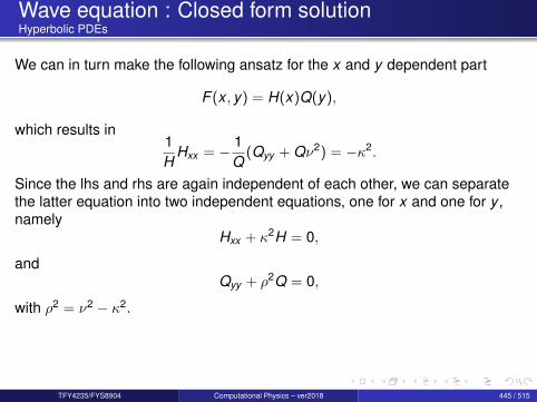
Wave equation : Closed form solutionHyperbolic PDEs
We can in turn make the following ansatz for the x and y dependent part
F (x , y) = H(x)Q(y),
which results in1H
Hxx = − 1Q
(Qyy + Qν2) = −κ2.
Since the lhs and rhs are again independent of each other, we can separatethe latter equation into two independent equations, one for x and one for y ,namely
Hxx + κ2H = 0,
andQyy + ρ2Q = 0,
with ρ2 = ν2 − κ2.
TFY4235/FYS8904 Computational Physics – ver2018 445 / 515

Wave equation : Closed form solutionHyperbolic PDEs
The second step is to solve these differential equations, which all havetrigonometric functions as solutions, viz.
H(x) = A cos(κx) + B sin(κx),
andQ(y) = C cos(ρy) + D sin(ρy).
The boundary conditions require that F (x , y) = H(x)Q(y) are zero at theboundaries, meaning that H(0) = H(L) = Q(0) = Q(L) = 0. This yields thesolutions
Hm(x) = sin(mπx
L) Qn(y) = sin(
nπyL
),
orFmn(x , y) = sin(
mπxL
) sin(nπy
L).
TFY4235/FYS8904 Computational Physics – ver2018 446 / 515

Wave equation : Closed form solutionHyperbolic PDEs
With ρ2 = ν2 − κ2 and λ = cν we have an eigenspectrum λ = c√κ2 + ρ2 or
λmn = cπ/L√
m2 + n2. The solution for G is
Gmn(t) = Bmn cos(λmnt) + Dmn sin(λmnt),
with the general solution of the form
u(x , y , t) =∞∑
mn=1
umn(x , y , t) =∞∑
mn=1
Fmn(x , y)Gmn(t).
TFY4235/FYS8904 Computational Physics – ver2018 447 / 515
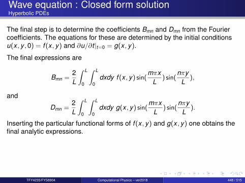
Wave equation : Closed form solutionHyperbolic PDEs
The final step is to determine the coefficients Bmn and Dmn from the Fouriercoefficients. The equations for these are determined by the initial conditionsu(x , y ,0) = f (x , y) and ∂u/∂t |t=0 = g(x , y).
The final expressions are
Bmn =2L
∫ L
0
∫ L
0dxdy f (x , y) sin(
mπxL
) sin(nπy
L),
and
Dmn =2L
∫ L
0
∫ L
0dxdy g(x , y) sin(
mπxL
) sin(nπy
L).
Inserting the particular functional forms of f (x , y) and g(x , y) one obtains thefinal analytic expressions.
TFY4235/FYS8904 Computational Physics – ver2018 448 / 515
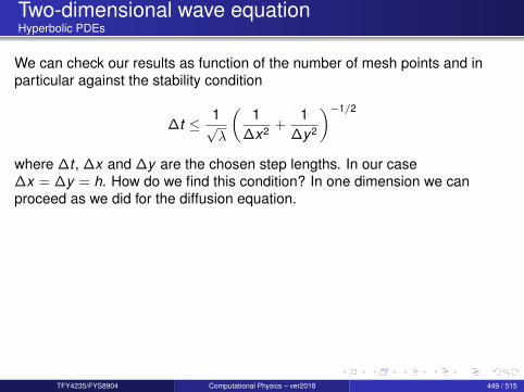
Two-dimensional wave equationHyperbolic PDEs
We can check our results as function of the number of mesh points and inparticular against the stability condition
∆t ≤ 1√λ
(1
∆x2 +1
∆y2
)−1/2
where ∆t , ∆x and ∆y are the chosen step lengths. In our case∆x = ∆y = h. How do we find this condition? In one dimension we canproceed as we did for the diffusion equation.
TFY4235/FYS8904 Computational Physics – ver2018 449 / 515
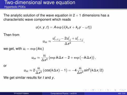
Two-dimensional wave equationHyperbolic PDEs
The analytic solution of the wave equation in 2 + 1 dimensions has acharacteristic wave component which reads
u(x , y , t) = A exp (i(kxx + ky y − ωt))
Then from
uxx ≈ul
i+1,j − 2uli,j + ul
i−1,j
∆x2 ,
we get, with ui = exp (ikxi )
uxx ≈ui
∆x2 (exp ik∆x − 2 + exp (−ik∆x)) ,
oruxx ≈ 2
ui
∆x2 (cos(k∆x)− 1) = −4ui
∆x2 sin2(k∆x/2)
We get similar results for t and y .
TFY4235/FYS8904 Computational Physics – ver2018 450 / 515
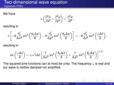
Two-dimensional wave equationHyperbolic PDEs
We have
λ
(∂2u∂x2 +
∂2u∂y2
)=∂2u∂t2 ,
resulting in
λ
[−4
ulij
∆x2 sin2(
kx ∆x2
)− 4
ulij
∆y2 sin2(
ky ∆y2
)]= −4
ulij
∆t2 sin2(ω∆t
2
),
resulting in
sin
(ω∆t
2
)= ±√λ∆t
[1
∆x2 sin2(
kx ∆x2
)+
1∆y2 sin2
(ky ∆y
2
)]1/2
.
The squared sine functions can at most be unity. The frequency ω is real andour wave is neither damped nor amplified.
TFY4235/FYS8904 Computational Physics – ver2018 451 / 515
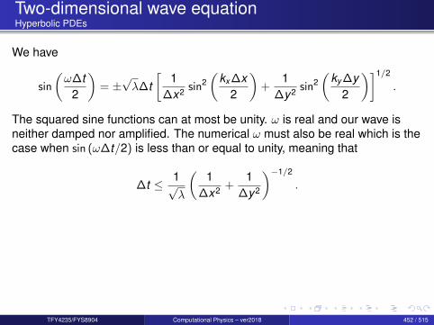
Two-dimensional wave equationHyperbolic PDEs
We have
sin
(ω∆t
2
)= ±√λ∆t
[1
∆x2 sin2(
kx ∆x2
)+
1∆y2 sin2
(ky ∆y
2
)]1/2
.
The squared sine functions can at most be unity. ω is real and our wave isneither damped nor amplified. The numerical ω must also be real which is thecase when sin (ω∆t/2) is less than or equal to unity, meaning that
∆t ≤ 1√λ
(1
∆x2 +1
∆y2
)−1/2
.
TFY4235/FYS8904 Computational Physics – ver2018 452 / 515

Two-dimensional wave equationHyperbolic PDEs
We modify now the wave equation in order to consider a 2 + 1 dimensionalwave equation with a position dependent velocity, given by
∂2u∂t2 = ∇ · (λ(x , y)∇u).
If λ is constant, we obtain the standard wave equation discussed in the twoprevious points. The solution u(x , y , t) could represent a model for waterwaves. It represents then the surface elevation from still water. We can modelλ as
λ = gH(x , y),
with g being the acceleration of gravity and H(x , y) is the still water depth.The function H(x , y) simulates the water depth using for examplemeasurements of still water depths in say a fjord or the north sea. Theboundary conditions are then determined by the coast lines as discussed inpoint d) below. We have assumed that the vertical motion is negligible andthat we deal with long wavelenghts λ compared with the depth of the sea H,that is λ/H 1. We neglect normally Coriolis effects in such calculations.
TFY4235/FYS8904 Computational Physics – ver2018 453 / 515
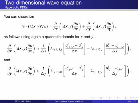
Two-dimensional wave equationHyperbolic PDEs
You can discretize
∇ · (λ(x , y)∇u) =∂
∂x
(λ(x , y)
∂u∂x
)+
∂
∂y
(λ(x , y)
∂u∂y
),
as follows using again a quadratic domain for x and y :
∂
∂x
(λ(x , y)
∂u∂x
)≈ 1
∆x
(λi+1/2,j
[ul
i+1,j − uli,j
∆x
]− λi−1/2,j
[ul
i,j − uli−1,j
∆x
]),
and
∂
∂y
(λ(x , y)
∂u∂y
)≈ 1
∆y
(λi,j+1/2
[ul
i,j+1 − uli,j
∆y
]− λi,j−1/2
[ul
i,j − uli,j−1
∆y
]).
TFY4235/FYS8904 Computational Physics – ver2018 454 / 515
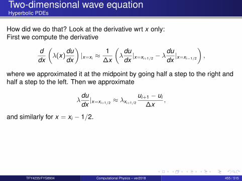
Two-dimensional wave equationHyperbolic PDEs
How did we do that? Look at the derivative wrt x only:First we compute the derivative
ddx
(λ(x)
dudx
)|x=xi ≈
1∆x
(λ
dudx|x=xi+1/2 − λ
dudx|x=xi−1/2
),
where we approximated it at the midpoint by going half a step to the right andhalf a step to the left. Then we approximate
λdudx|x=xi+1/2 ≈ λxi+1/2
ui+1 − ui
∆x,
and similarly for x = xi − 1/2.
TFY4235/FYS8904 Computational Physics – ver2018 455 / 515
Elliptic PDEs
TFY4235/FYS8904 Computational Physics – ver2018 456 / 515

Laplace’s and Poisson’s equationsElliptic PDEs
Laplace’s equation (in 2 spatial dimensions) reads
∇2u(x) = uxx + uyy = 0.
with possible boundary conditions u(x , y) = g(x , y) on the border. There is notime-dependence. Choosing equally many steps in both directions we have aquadratic or rectangular grid, depending on whether we choose equal stepslengths or not in the x and the y directions. Here we set ∆x = ∆y = h andobtain a discretized version
uxx ≈u(x + h, y)− 2u(x , y) + u(x − h, y)
h2 ,
and
uyy ≈u(x , y + h)− 2u(x , y) + u(x , y − h)
h2 ,
TFY4235/FYS8904 Computational Physics – ver2018 457 / 515

Laplace’s and Poisson’s equationsElliptic PDEs
uxx ≈ui+1,j − 2ui,j + ui−1,j
h2 ,
and
uyy ≈ui,j+1 − 2ui,j + ui,j−1
h2 ,
which gives when inserted in Laplace’s equation
ui,j =14[ui,j+1 + ui,j−1 + ui+1,j + ui−1,j
]. (5)
This is our final numerical scheme for solving Laplace’s equation. Poisson’sequation adds only a minor complication to the above equation since in thiscase we have
uxx + uyy = −ρ(x),
and we need only to add a discretized version of ρ(x) resulting in
ui,j =14[ui,j+1 + ui,j−1 + ui+1,j + ui−1,j
]+ ρi,j . (6)
TFY4235/FYS8904 Computational Physics – ver2018 458 / 515
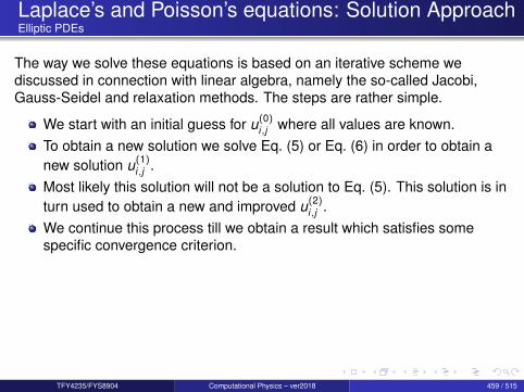
Laplace’s and Poisson’s equations: Solution ApproachElliptic PDEs
The way we solve these equations is based on an iterative scheme wediscussed in connection with linear algebra, namely the so-called Jacobi,Gauss-Seidel and relaxation methods. The steps are rather simple.
We start with an initial guess for u(0)i,j where all values are known.
To obtain a new solution we solve Eq. (5) or Eq. (6) in order to obtain anew solution u(1)
i,j .Most likely this solution will not be a solution to Eq. (5). This solution is inturn used to obtain a new and improved u(2)
i,j .We continue this process till we obtain a result which satisfies somespecific convergence criterion.
TFY4235/FYS8904 Computational Physics – ver2018 459 / 515

Code example for the two-dimensional diffusionequation/Laplace
i n t Di f f us i onJacob i ( i n t N, double dx , double dt ,double ∗∗A, double ∗∗q , double abs to l )
i n t i , j , k ;i n t maxit = 100000;double sum ;double ∗∗ Aold = CreateMatr ix (N,N) ;
double D = dt / ( dx∗dx ) ;
TFY4235/FYS8904 Computational Physics – ver2018 460 / 515

Code example for the two-dimensional diffusionequation/Laplace
for ( i =1; i<N−1; i ++)for ( j =1; j<N−1; j ++)
Aold [ i ] [ j ] = 1 . 0 ;/∗ Boundary Condi t ions −− a l l zeros ∗ /for ( i =0; i<N; i ++)
A [ 0 ] [ i ] = 0 . 0 ;A [N−1][ i ] = 0 . 0 ;A [ i ] [ 0 ] = 0 . 0 ;A [ i ] [ N−1] = 0 . 0 ;
TFY4235/FYS8904 Computational Physics – ver2018 461 / 515
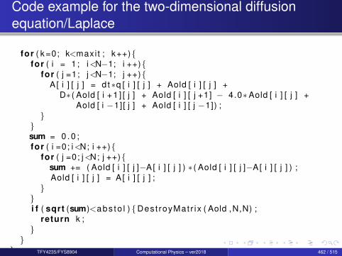
Code example for the two-dimensional diffusionequation/Laplace
for ( k =0; k<maxit ; k++)for ( i = 1 ; i<N−1; i ++)
for ( j =1; j<N−1; j ++)A[ i ] [ j ] = d t ∗q [ i ] [ j ] + Aold [ i ] [ j ] +
D∗ ( Aold [ i + 1 ] [ j ] + Aold [ i ] [ j +1] − 4.0∗Aold [ i ] [ j ] +Aold [ i −1][ j ] + Aold [ i ] [ j −1]) ;
sum = 0 . 0 ;for ( i =0; i<N; i ++)
for ( j =0; j<N; j ++)sum += ( Aold [ i ] [ j ]−A[ i ] [ j ] ) ∗ ( Aold [ i ] [ j ]−A[ i ] [ j ] ) ;Aold [ i ] [ j ] = A [ i ] [ j ] ;
i f ( sqrt (sum)<abs to l ) Dest royMatr ix ( Aold ,N,N) ;
return k ;
TFY4235/FYS8904 Computational Physics – ver2018 462 / 515

Other methods
TFY4235/FYS8904 Computational Physics – ver2018 463 / 515

Other methods
Other methodsFinite-element methodBoundary element methods
TFY4235/FYS8904 Computational Physics – ver2018 464 / 515

Section 12
Optimization
TFY4235/FYS8904 Computational Physics – ver2018 465 / 515

Outline I
1 Introduction
2 Number representation and numerical precision
3 Finite differences and interpolation
4 Linear algebra
5 How to install libraries on a Linux system
6 Eigenvalue problems
7 Spectral methods
8 Numerical integration
TFY4235/FYS8904 Computational Physics – ver2018 466 / 515

Outline II9 Random numbers
10 Ordinary differential equations
11 Partial differential equations
12 OptimizationOptimization in one dimensionsBisection methodDownhill simplex methodConjugate gradient methodsQuasi-Newton methodχ2-minimizationGenetic algorithmsConstrained Optimization: Linear programmingConstrained Optimization: Non-Linear programmingSimulated annealing
TFY4235/FYS8904 Computational Physics – ver2018 467 / 515
Optimization (minimization/maximization)Introduction
Some initial comments:Optimization is a wide field.Sometimes there exists a well-established method that can be used in ablack-box mannerbut many optimization problems are true challenges
Note :Maximizing f (x) is equivalent to minimizing −f (x)!It is intimately related to methods of solving non-linear equations (for∇f (x) = 0).
TFY4235/FYS8904 Computational Physics – ver2018 468 / 515

Optimization (minimization/maximization)Introduction
To minimize a function f (x) in D dimensions, x ∈ RD, one has to considerseveral issues:
What is the dimensionality D?Are there constraints on x?Is the problem linear or non-linear?Is f (x) such that minimization is a smooth downhill process, or are theretraps in the form of local minima?Do we want the global minimum of f (x) , or is it sufficient to make a localminimization?Do we have access to derivatives of f (x)?
TFY4235/FYS8904 Computational Physics – ver2018 469 / 515
Optimization (minimization/maximization)Introduction
Some classes of optimization problems with examples of related methods
Global optimizationSimulated annealing
Local optimization without derivativesBisection methodDownhill simplex method
Local optimization with derivativesQuasi-NewtonConjugate gradient
Constrained optimizationLinear programmingNon-linear programming
TFY4235/FYS8904 Computational Physics – ver2018 470 / 515

Optimization (minimization/maximization)Introduction
General remark on precision: Let xm be the true minimum of the function f (x)[we assume D = 1], so that
f (x) ≈ f (xm) +12
(x − xm)2f ′′(xm); or f (x)− f (xm) ≈ 12
(x − xm)2f ′′(xm)
If |x − xm| is so small that |f (x)− f (xm)| is of the order the floating-pointprecision, ε, one cannot expect to get closer to xm by any methodThis gives an estimate of the error in an estimate x for the minimumxm = x ±∆x
ε ≈ f (x)− f (xm) ≈ 12
(x − xm)2f ′′(xm)
so that the error in xm becomes
∆xm ≥√ε
√2f (xm)
f ′′(xm)
The error in xm (∼ √ε) is typically much larger then the error in f (xm) (∼ ε)!TFY4235/FYS8904 Computational Physics – ver2018 471 / 515
Optimization in one dimensionsOptimization
For one-dimensional optimization, there exist several methods that are bothrelatively robust and fast!
Some examples are:BracketingBisection methodGolden searchBrent’s method (parabolic interpolation)Newtons method
TFY4235/FYS8904 Computational Physics – ver2018 472 / 515
Bisection methodOptimization
Alex covered this....!Newtons methods also works well for one-dimensions.
TFY4235/FYS8904 Computational Physics – ver2018 473 / 515

Newton’s methodOptimization
Taylor expansion gives
f (x) ≈ f (xn) + f ′(xn)(x − xn) +12
f ′′(xn)(x − xn)2 + . . .
Neglecting terms of second order in x gives
f (xn+1) ≈ 0 f (xn) + f ′(xn)(xn+1 − xn) ≈ 0
which results in the the iteration scheme
xn+1 = xn −f (xn)
f ′(xn)
This is Newton’s method also known as NewtonRaphson method.
TFY4235/FYS8904 Computational Physics – ver2018 474 / 515

Downhill simplex methodOptimization
The Downhill simplex method is an example of local optimization withoutderivatives in multi-dimensions!does not rely on information on the gradientviewed as a generalization of bracketing to multi-dimensions
A simplex in D dimensions is a geometrical object defined by D + 1 vertices.D = 1 : a line segmentD = 2 : a triangleD = 3 : a tetrahedronetc.
A simplex is a dynamical object that can grow and shrink; When it reaches theminimum, it gives up and shrinks down around it.
The simplex method is iterative!
TFY4235/FYS8904 Computational Physics – ver2018 475 / 515

Downhill simplex methodOptimization
The Downhill simplex method consists of the following steps1 Start from a simplex defined by vertices x1, x2, . . . xD+1 defined so that
f (x1) ≥ f (x2) ≥ . . . ≥ f (xD+1).
2 Elementary move: Improve the worst point, i.e. x1, by moving in directionof the mean of the better points
xmean =1D
D+1∑i=2
x i
by trying
xa = xmean + λ(xmean − x1)
for some λ ∈ R and xa → x1 if improved.Illustrationhttps://notendur.hi.is/jonasson/olbest/sim-anneal1.pdf
TFY4235/FYS8904 Computational Physics – ver2018 476 / 515
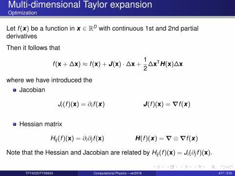
Multi-dimensional Taylor expansionOptimization
Let f (x) be a function in x ∈ RD with continuous 1st and 2nd partialderivatives
Then it follows that
f (x + ∆x) ≈ f (x) + J(x) ·∆x +12
∆xTH(x)∆x
where we have introduced theJacobian
Ji (f )(x) = ∂i f (x) J(f )(x) = ∇f (x)
Hessian matrix
Hij (f )(x) = ∂i∂j f (x) H(f )(x) = ∇⊗∇f (x)
Note that the Hessian and Jacobian are related by Hij (f )(x) = Ji (∂j f )(x).
TFY4235/FYS8904 Computational Physics – ver2018 477 / 515

Multi-dimensional Taylor expansionOptimization
The Hessian matrix corresponding to the function f (x) written out in detail:
H(f ) =
∂2f∂x2
1
∂2f∂x1 ∂x2
· · · ∂2f∂x1 ∂xn
∂2f∂x2 ∂x1
∂2f∂x2
2· · · ∂2f
∂x2 ∂xn
......
. . ....
∂2f∂xn ∂x1
∂2f∂xn ∂x2
· · · ∂2f∂x2
n
.
TFY4235/FYS8904 Computational Physics – ver2018 478 / 515

Multi-dimensional Taylor expansionOptimization
Minimizing the function f (x) in D-dimensions, can be viewed as solving∇f (x) = 0, which is a system of D generally non-linear equations
One has
f (x ′) = f (x) + ∇f (x) · (x ′ − x) +12
(x ′ − x)T H(x)(x ′ − x) + . . .
Now taking the gradient with respect to primed coordinates gives
∇′f (x ′) = ∇f (x) + H(x)(x ′ − x) + . . .
If the true minimum is at x ′, so that ∇′f (x ′) = 0, one has after neglectinghigher order terms
H(x)(x ′ − x) = −∇f (x),
that is, a linear system in δx = x ′ − x with the Hessian being the systemmatrix and b = −∇f (x) being the right-hand-side!
Methods from solving linear systems can be used for minimizing functions!TFY4235/FYS8904 Computational Physics – ver2018 479 / 515

Conjugate gradient methodOptimization
For instance, if the Hessian is available, we could solve the linear system
H(x)(x ′ − x) = −∇f (x)
to find the minimum x ′ by the use of the conjugate gradient method that wehave seen previously.
Note that the Hessian (for a well-behaved function) is symmetric as required!
We will therefore not discuss this further here!
TFY4235/FYS8904 Computational Physics – ver2018 480 / 515
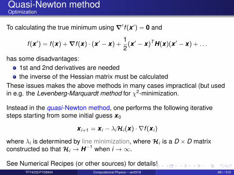
Quasi-Newton methodOptimization
To calculating the true minimum using ∇′f (x ′) = 0 and
f (x ′) = f (x) + ∇f (x) · (x ′ − x) +12
(x ′ − x)T H(x)(x ′ − x) + . . .
has some disadvantages:1st and 2nd derivatives are neededthe inverse of the Hessian matrix must be calculated
These issues makes the above methods in many cases impractical (but usedin e.g. the Levenberg-Marquardt method for χ2-minimization.
Instead in the quasi-Newton method, one performs the following iterativesteps starting from some initial guess x0
x i+1 = x i − λiHi (x) · ∇f (x i )
where λi is determined by line minimization, where Hi is a D × D matrixconstructed so that Hi → H−1 when i →∞.
See Numerical Recipes (or other sources) for details!TFY4235/FYS8904 Computational Physics – ver2018 481 / 515

Quasi-Newton methodOptimization
Quasi-Newton (or variable metric methods) in muti-dimensions come in twoflavors (which only differ in some minor details):
Broyden-Fletcher-Goldfarb-Shanno (BFGS) algorithmhttp://en.wikipedia.org/wiki/BFGS_method
Davidon-Fletcher-Powell (DFP) formulahttp://en.wikipedia.org/wiki/DFP_updating_formula
other variantshttp://en.wikipedia.org/wiki/Quasi-Newton_method
The main idea is to base iterations on the multi-dimensional Taylor expansion,but using an approximate Hessian constructed “as one goes”!In quasi-Newton methods the Hessian matrix does not need to be computed.The Hessian is updated by analyzing successive gradient vectors instead.
Comments : In practical applications, the BFGS approach seems to bepreferred!
TFY4235/FYS8904 Computational Physics – ver2018 482 / 515
Quasi-Newton methodOptimization
Some commentsThe quasi-Newton method is often comparable in efficiency to theconjugate-gradient methodHowever it requires more memory if D is largeMemory requirement scales as D2 for the quasi-Newton method and asD for the conjugate-gradient method.Unlike the conjugate-gradient method, the quasi-Newton methods do notrequire the Hessian matrix to be evaluated directly.
TFY4235/FYS8904 Computational Physics – ver2018 483 / 515
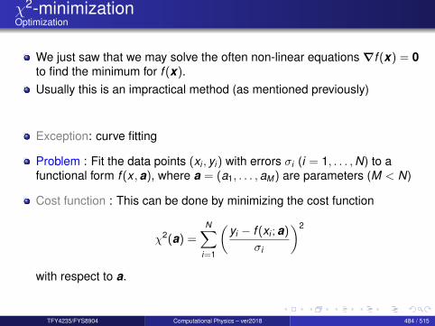
χ2-minimizationOptimization
We just saw that we may solve the often non-linear equations ∇f (x) = 0to find the minimum for f (x).Usually this is an impractical method (as mentioned previously)
Exception: curve fitting
Problem : Fit the data points (xi , yi ) with errors σi (i = 1, . . . ,N) to afunctional form f (x ,a), where a = (a1, . . . ,aM) are parameters (M < N)
Cost function : This can be done by minimizing the cost function
χ2(a) =N∑
i=1
(yi − f (xi ; a)
σi
)2
with respect to a.
TFY4235/FYS8904 Computational Physics – ver2018 484 / 515
χ2-minimizationOptimization
Two possibilitiesLinear problems : f (x ; a) depends linearly on ai for all i .Non-linear problems : f (x ; a) depends non-linearly on ai .
Levenberg-Marquardt algorithm
The linear problems result in a linear system of equations that is simple tosolve; the non-linear problem is harder!
TFY4235/FYS8904 Computational Physics – ver2018 485 / 515
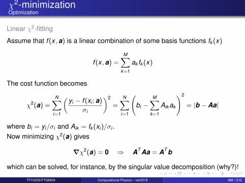
χ2-minimizationOptimization
Linear χ2-fitting
Assume that f (x ,a) is a linear combination of some basis functions fk (x)
f (x ,a) =M∑
k=1
ak fk (x)
The cost function becomes
χ2(a) =N∑
i=1
(yi − f (xi ; a)
σi
)2
=N∑
i=1
(bi −
M∑k=1
Aik ak
)2
= |b − Aa|
where bi = yi/σi and Aik = fk (xi )/σi .Now minimizing χ2(a) gives
∇χ2(a) = 0 ⇒ AT Aa = AT b
which can be solved, for instance, by the singular value decomposition (why?)!
TFY4235/FYS8904 Computational Physics – ver2018 486 / 515
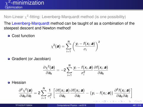
χ2-minimizationOptimization
Non-Linear χ2-fitting: Levenberg-Marquardt method (is one possibility)
The Levenberg-Marquardt method can be taught of as a combination of thesteepest descent and Newton method!
Cost function
χ2(a) =N∑
i=1
(yi − f (xi ; a)
σi
)2
Gradient (or Jacobian)
∂χ2(a)
∂ak= −2
N∑i=1
yi − f (xi ,a)
σ2i
∂f (xi ; a)
∂ak
Hessian
∂2χ2(a)
∂ak∂al= 2
N∑i=1
1σ2
i
[∂f (xi ; a)
∂ak
∂f (xi ; a)
∂al− yi − f (xi ; a) ∂
2f (xi ; a)
∂ak∂al
]TFY4235/FYS8904 Computational Physics – ver2018 487 / 515

χ2-minimizationOptimization
Hessian (continued): The last term of the Hessian should be small if weare near the minimum (so that the fit is good). Note that it vanishesexactly if f depends linearly on ai .For convenience, this term is neglected to give an approximate Hessian
∂2χ2(a)
∂ak∂al≈ Akl = 2
N∑i=1
1σ2
i
∂f (xi ; a)
∂ak
∂f (xi ; a)
∂al
Defining
βk = −12∂χ2(a)
∂akαkl =
12
Akl =12∂2χ2(a)
∂ak∂alδak = a′k − ak
A steepest decent step would be δak = const βk , but the LM-methoduses a modified steepest decent step
TFY4235/FYS8904 Computational Physics – ver2018 488 / 515
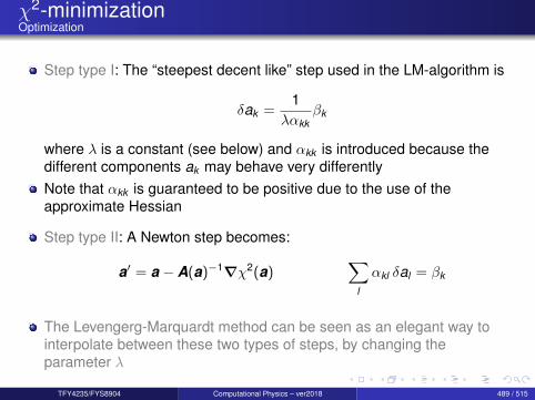
χ2-minimizationOptimization
Step type I: The “steepest decent like” step used in the LM-algorithm is
δak =1
λαkkβk
where λ is a constant (see below) and αkk is introduced because thedifferent components ak may behave very differentlyNote that αkk is guaranteed to be positive due to the use of theapproximate Hessian
Step type II: A Newton step becomes:
a′ = a − A(a)−1∇χ2(a)∑
l
αkl δal = βk
The Levengerg-Marquardt method can be seen as an elegant way tointerpolate between these two types of steps, by changing theparameter λ
TFY4235/FYS8904 Computational Physics – ver2018 489 / 515

χ2-minimizationOptimization
This is achieved by considering the following “LM-equation system”
∑l
αkl δal = βl αkl =
αkk (1 + λ) k = lαkl k 6= l
Observations
λ→ 0 : a Newton step because αkl and αkl are the same in this limit
λ 1 (or λ→∞): modified Steepest decent step because the diagonalelements dominates the matrix αkl
TFY4235/FYS8904 Computational Physics – ver2018 490 / 515
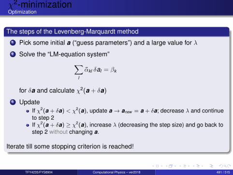
χ2-minimizationOptimization
The steps of the Levenberg-Marquardt method1 Pick some initial a (“guess parameters”) and a large value for λ
2 Solve the “LM-equation system”∑l
αkl δal = βk
for δa and calculate χ2(a + δa)
3 UpdateIf χ2(a + δa) < χ2(a), update a → anew = a + δa; decrease λ and continueto step 2If χ2(a + δa) ≥ χ2(a), increase λ (decreasing the step size) and go back tostep 2 without changing a.
Iterate till some stopping criterion is reached!
TFY4235/FYS8904 Computational Physics – ver2018 491 / 515

χ2-minimizationOptimization
The steps of the Levenberg-Marquardt method1 Pick some initial a (“guess parameters”) and a large value for λ
2 Solve the “LM-equation system”∑l
αkl δal = βk
for δa and calculate χ2(a + δa)
3 UpdateIf χ2(a + δa) < χ2(a), update a → anew = a + δa; decrease λ and continueto step 2If χ2(a + δa) ≥ χ2(a), increase λ (decreasing the step size) and go back tostep 2 without changing a.
Iterate till some stopping criterion is reached!
TFY4235/FYS8904 Computational Physics – ver2018 492 / 515
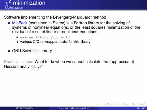
χ2-minimizationOptimization
Software implementing the Levengerg-Marquardt methodMinPack (contained in Slatec) is a Fortran library for the solving ofsystems of nonlinear equations, or the least squares minimization of theresidual of a set of linear or nonlinear equations.
www.netlib.org/minpack/various C/C++ wrappers exist for this library
GNU Scientific Library
Practical issues: What to do when we cannot calculate the (approximate)Hessian analytically?
TFY4235/FYS8904 Computational Physics – ver2018 493 / 515

χ2-minimizationOptimization
Numerical examples
To appear later....
TFY4235/FYS8904 Computational Physics – ver2018 494 / 515

Genetic algorithmsOptimization
To appear later....
TFY4235/FYS8904 Computational Physics – ver2018 495 / 515

Constrained Optimization: Linear programmingOptimization
To appear later....
TFY4235/FYS8904 Computational Physics – ver2018 496 / 515

Constrained Optimization: Non-Linear programmingOptimization
To appear later....
TFY4235/FYS8904 Computational Physics – ver2018 497 / 515
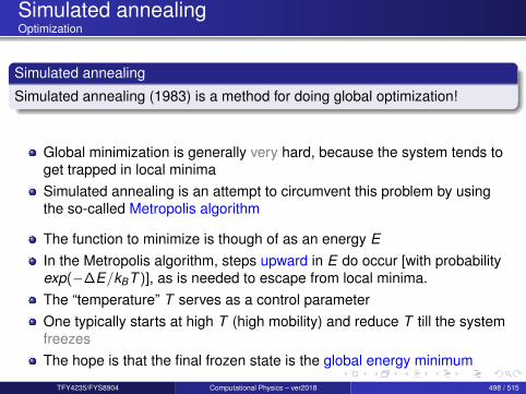
Simulated annealingOptimization
Simulated annealing
Simulated annealing (1983) is a method for doing global optimization!
Global minimization is generally very hard, because the system tends toget trapped in local minimaSimulated annealing is an attempt to circumvent this problem by usingthe so-called Metropolis algorithm
The function to minimize is though of as an energy EIn the Metropolis algorithm, steps upward in E do occur [with probabilityexp(−∆E/kBT )], as is needed to escape from local minima.The “temperature” T serves as a control parameterOne typically starts at high T (high mobility) and reduce T till the systemfreezesThe hope is that the final frozen state is the global energy minimum
TFY4235/FYS8904 Computational Physics – ver2018 498 / 515

The Metropolis algorithm (1953)
TFY4235/FYS8904 Computational Physics – ver2018 499 / 515

Recall from Statistical PhysicsOptimization
Consider a system that can be found in many different states x (e.g. a systemof N spins siJ1,NK), x = (s1, · · · , sN) is the state vector of spins.
We want to compute a thermal average of some quantity A (e.g. the averagespin).We know from statistical physics that in thermal equilibrium this average isgiven by:
〈A〉 =1Z
∑x
A(x)e−H(x )/T =∑x
A(x)PB(x)
T : temperature;H(x): Hamiltonian of the system in state x ;Z =
∑x e−H(x )/kBT is the partition function;
PB(x) =[e−H(x )/kBT
]/Z is the Boltzmann distribution;
kB is the Boltzmann constant.
TFY4235/FYS8904 Computational Physics – ver2018 500 / 515
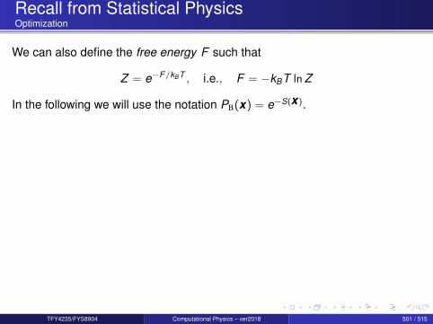
Recall from Statistical PhysicsOptimization
We can also define the free energy F such that
Z = e−F/kBT , i.e., F = −kBT ln Z
In the following we will use the notation PB(x) = e−S(x ).
TFY4235/FYS8904 Computational Physics – ver2018 501 / 515
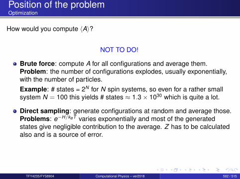
Position of the problemOptimization
How would you compute 〈A〉?
NOT TO DO!
Brute force: compute A for all configurations and average them.Problem: the number of configurations explodes, usually exponentially,with the number of particles.Example: # states = 2N for N spin systems, so even for a rather smallsystem N = 100 this yields # states ≈ 1.3× 1030 which is quite a lot.
Direct sampling: generate configurations at random and average those.Problems: e−H/kBT varies exponentially and most of the generatedstates give negligible contribution to the average. Z has to be calculatedalso and is a source of error.
TFY4235/FYS8904 Computational Physics – ver2018 502 / 515
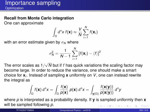
Importance samplingOptimization
Recall from Monte Carlo integrationOne can approximate ∫
Ω
dnx f (x) ≈ VN
N∑i=1
f (xi )
with an error estimate given by σN where
σ2N =
1N − 1
N∑i=1
[f (xi )− 〈f 〉]2
The error scales as 1/√
N but if f has quick variations the scaling factor maybecome large. In order to reduce the variance, one should make a smartchoice for xi . Instead of sampling x uniformly on V , one can instead rewritethe integral as∫
Ω
f (x) dnx =
∫Ω
f (x)
p(x)p(x) dnx =
∫y(Ω)
f (x(y))
p(x(y))dny
where p is interpreted as a probability density. If y is sampled uniformly then xwill be sampled following p.
TFY4235/FYS8904 Computational Physics – ver2018 503 / 515

Importance samplingOptimization
This yields
〈f 〉 =1N
N∑i=1
f (xi )
p(xi )
with the error estimated by
σ2N =
1N − 1
N∑i=1
[f (xi )
p(xi )−⟨
fp
⟩]2
Then the variance is reduced if f/p is slowly varying.
The idea here: generate configuration according to the Boltzmanndistribution. The difficult part is then to draw states following the Boltzmanndistribution. A method to do this is the Metropolis algorithm.
TFY4235/FYS8904 Computational Physics – ver2018 504 / 515
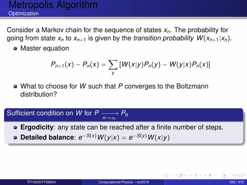
Metropolis AlgorithmOptimization
Consider a Markov chain for the sequence of states xn. The probability forgoing from state xn to xn+1 is given by the transition probability W (xn+1|xn).
Master equation
Pn+1(x)− Pn(x) =∑
y
[W (x |y)Pn(y)−W (y |x)Pn(x)]
What to choose for W such that P converges to the Boltzmanndistribution?
Sufficient condition on W for P −−−→n→∞
PB
Ergodicity: any state can be reached after a finite number of steps.Detailed balance: e−S(x)W (y |x) = e−S(y)W (x |y)
TFY4235/FYS8904 Computational Physics – ver2018 505 / 515
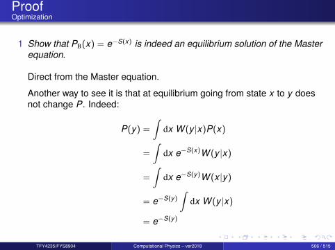
ProofOptimization
1 Show that PB(x) = e−S(x) is indeed an equilibrium solution of the Masterequation.
Direct from the Master equation.
Another way to see it is that at equilibrium going from state x to y doesnot change P. Indeed:
P(y) =
∫dx W (y |x)P(x)
=
∫dx e−S(x)W (y |x)
=
∫dx e−S(y)W (x |y)
= e−S(y)
∫dx W (y |x)
= e−S(y)
TFY4235/FYS8904 Computational Physics – ver2018 506 / 515

ProofOptimization
2 Show that Pn converges to PB. For this we need a measure for theconvergence. Consider ‖Pn − PB‖ =
∫dx |Pn(x)− e−S(x)|.
‖Pn+1 − PB‖ =
∫dy |Pn+1(y)− e−S(y)|
=
∫dy |
∫dx Pn(x)W (y |x)− e−S(y)|
=
∫dy |
∫dx[Pn(x)W (y |x)− e−S(y)W (x |y)
]|
=
∫dy |
∫dx[Pn(x)W (y |x)− e−S(x)W (y |x)
]|
=
∫dy |
∫dx[Pn(x)− e−S(x)
]W (y |x)|
≤∫
dy∫
dx |Pn(x)− e−S(x)|W (y |x)
≤∫
dx |Pn(x)− e−S(x)| = ‖Pn − PB‖
TFY4235/FYS8904 Computational Physics – ver2018 507 / 515
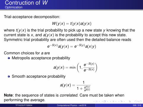
Contruction of WOptimization
Trial-acceptance decomposition:
W (y |x) = t(y |x)a(y |x)
where t(y |x) is the trial probability to pick up a new state y knowing that thecurrent state is x , and a(y |x) is the probability to accept this new state.Symmetric trial probability are often used then the detailed balance reads
e−S(x)a(y |x) = e−S(y)a(x |y)
Common choices for a areMetropolis acceptance probability
a(y |x) = min
(1,
e−S(y)
e−S(x)
)Smooth acceptance probability
a(y |x) =1
1 + eS(y)
eS(x)
Note: the sequence of states is correlated. Care must be taken whenperforming the average.
TFY4235/FYS8904 Computational Physics – ver2018 508 / 515

Monte Carlo using Metropolis algorithmOptimization
Monte Carlo using Metropolis algorithm1 Start from an initial state x = x0.2 Draw a new state x according to the trial probability t(x |xn).3 Accept the new state with probability a(x |xn) satisfying the detailed
balance:if accepted set: xn+1 ← xif rejected set: xn+1 ← xn
4 Repeat steps 2–3 until equilibrium is reached and enough data havebeen generated. Discard non-equilibrium steps for the averaging.
QuestionsHow do we know when equilibrium is reached?How much data must be collected?
TFY4235/FYS8904 Computational Physics – ver2018 509 / 515
Example: Ising modelOptimization
The Ising modelConsider a system of N spins, where each spin si is located at position i on ad-dimensional cubic lattice. Each spin can take the value ±1.
The Hamiltonian of the system is
H = −J∑〈i,j〉
sisj
where J is the coupling constant and∑〈i,j〉 denotes a sum over all
nearest-neighbour pair of sites.
We are interested in the magnetization. At thermal equilibrium themagnetization M is given by
M =
∑states
∑i sie−H/T∑
states e−H/T
TFY4235/FYS8904 Computational Physics – ver2018 510 / 515
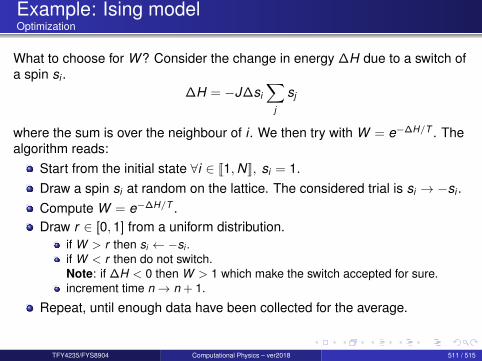
Example: Ising modelOptimization
What to choose for W? Consider the change in energy ∆H due to a switch ofa spin si .
∆H = −J∆si
∑j
sj
where the sum is over the neighbour of i . We then try with W = e−∆H/T . Thealgorithm reads:
Start from the initial state ∀i ∈ J1,NK, si = 1.Draw a spin si at random on the lattice. The considered trial is si → −si .Compute W = e−∆H/T .Draw r ∈ [0,1] from a uniform distribution.
if W > r then si ← −si .if W < r then do not switch.Note: if ∆H < 0 then W > 1 which make the switch accepted for sure.increment time n→ n + 1.
Repeat, until enough data have been collected for the average.
TFY4235/FYS8904 Computational Physics – ver2018 511 / 515

Example: Ising modelOptimization
0 5 10 15 20 25 30
5
10
15
20
25
30
(a) Initial config. T = Tc/20 5 10 15 20 25 30
5
10
15
20
25
30
(b) Initial config. T = 3Tc/2
0 5 10 15 20 25 30
5
10
15
20
25
30
(c) Equilibrium. T = Tc/20 5 10 15 20 25 30
5
10
15
20
25
30
(d) Equilibrium. T = 3Tc/2
Figure: Spin lattice. Lattice size L = 30, 400 sweeps.
TFY4235/FYS8904 Computational Physics – ver2018 512 / 515
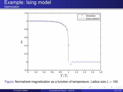
Example: Ising modelOptimization
0 0.2 0.4 0.6 0.8 1 1.2 1.4 1.6 1.8−0.2
0
0.2
0.4
0.6
0.8
1
1.2
T/Tc
m
SimulationExact solution
Figure: Normalized magnetization as a function of temperature. Lattice size L = 100.
TFY4235/FYS8904 Computational Physics – ver2018 513 / 515
Some commentsOptimization
How to average in a proper way?Eliminate boundary effects by using periodic boundary condition.When selecting a spin, do it randomly, not sequentially!The Monte Carlo time step should not be taken as a one switch of spin.An appropriate MC time that should be considered is one under which, onaverage, all spins have been attempted. This is also called a MC sweep.Discard a sufficient number of MC sweeps before collecting data foraverages. This avoid the average to be biased by initial configurationsthat are far away from the equilibrium.It is also a good idea to only average on every other sweep or so, in orderto reduce correlation between consecutive steps. But do not throw awaymost of your data for that purpose.Assuming a run gives Nsweep uncorrelated sweep to average over, makeNrun runs to estimate error as
∆A =σ√Nrun
How to speed it up?Make a table of possible w = e−∆H/T and look it up instead of computingthe same thing all the time.TFY4235/FYS8904 Computational Physics – ver2018 514 / 515
Importance sampling for the energyOptimization
In statistical physics, one is often interested in the partition function Z ,because many quantities can be deduced from it. Example:
〈E〉 =1Z
∑x
H(x)e−H(x)/T = −T 2 ddT
ln Z
Rather than summing over all states, one may sum over all energies:
Z =∑
x
e−H(x)/T =∑
E
g(E)e−E/T
where g is the density of states.
TFY4235/FYS8904 Computational Physics – ver2018 515 / 515