TFY4305 solutions extra exercises2014

Problem 2.3.3

Tumor growth can be modelled by Gompertz’ law

N = −aN ln(bN) , (1)

where N(t) is proportional to the number of cells in the tumor, and a, b > 0 are parameters.

a) In order to interpret b we note that N = 1/b is a stable fixed point since f(1/b) = 0and f(N) = −aN ln(bN) > 0 for N < 1/b and f(N) < 0 for N > 1/b. Thus 1/b is the lim-iting size of the tumor. The parameter a is related to the proliferation ability (cell division)and depends on the availability of substrate, oxygen etc.

Interestingly the Gompertz equation can be solved exactly. Separation of variables gives

dN

N ln bN= −adt (2)

Integration yields

ln[ln(bN)] = −at+ C , (3)

where C is an integration constant. Exponentiating this expression twice gives

N(t) =1

bee

Ce−at

. (4)

Using the initial condition N(0) = N0, one finds N0 = 1bee

Cor ln(N0b) = eC . The solution

can then be written as

N(t) =1

beln(N0b)e−at

. (5)

The solution satisfies N(0) = N0 and

limt→∞

=1

b. (6)

1

2

æç

0.5 1.0 1.5 2.0N

-2

-1

1

2

fHN L

Figure 1: Vector field for the Gompertz model with b = 1.

We can also gain insight into the solution without knowing it. Taking the derivative ofthe Gompertz equation, we obtain

N = −aN(ln(bN) + 1)

= a2N ln(bN)(ln(bN) + 1) . (7)

Assume first that N0 > 1/b. Then we know that N(t) decreases monotonically to N = 1/bas t→∞. In this case N < 0 and so N > 0. This implies that there is no inflection point.Next assume that N0 < 1/b. Then we that N(t) increases monotonically to N = 1/b ast → ∞. In this case N < 0 but N changes sign at N = 1

be−1. Thus there is an inflection

point here.

b) The other fixed point of the differential equation is N = 0 and this fixed point isunstable. The vector field is shown in Fig. 1 for b = 1. The graph N(t) is shown fora = b = 1 and two initial conditions N0 = 1/20 < 1/b and N0 = 1.2 > 1/b in Fig. 2. In theformer case one can clearly see the inflection point as predicted above.

3

0 1 2 3 4 5t

0.2

0.4

0.6

0.8

1.0

1.2

N HtL

Figure 2: Solution N(t) for a = 1 and two initial conditions N0 = 1/20 < 1/b and N0 =1.2 > 1/b.

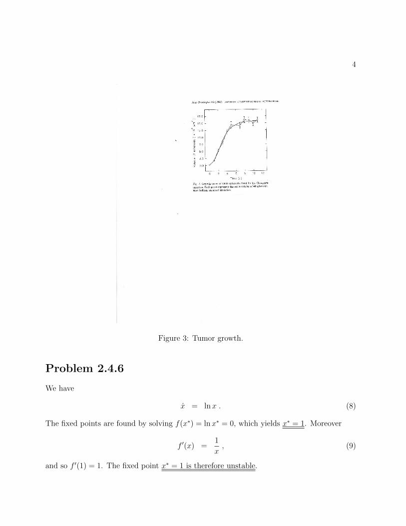
Fig. 3 shows the data points for tumor growth in a laboratory experiment at NTNU. Theparameters a and b have been fitted to the data points. The agreement is very good.

4

Figure 3: Tumor growth.

Problem 2.4.6

We have

x = lnx . (8)

The fixed points are found by solving f(x∗) = ln x∗ = 0, which yields x∗ = 1. Moreover

f ′(x) =1

x, (9)

and so f ′(1) = 1. The fixed point x∗ = 1 is therefore unstable.

5

Problem 2.6.1

The point is that the harmonic oscillator is not a first-order system. It is a system of twocoupled differential equations. Define x = y. This yields

my = −kx (10)

x = y , (11)

and we conclude that the system is two dimensional and so does not correspond to flow onthe line.

Problem 2.7.5

The dynamics is governed by the equation

x = − sinhx . (12)

The function f(x) = − sinhx is shown in Fig. 4. The only zero of f(x), i. e. fixed point is

> <è> <

-2 -1 1 2

x

-3

-2

-1

1

2

3

fHxL

Figure 4: Function f(x) = − sinhx.

x = 0. Since f ′(x) = − coshx and f ′(0) = −1, the fixed point is stable. This can also beinferred from inspecting the graph.

The potential is given by integration of dV/dx = sinhx, Integration yields

V (x) = coshx+ C , (13)

where C is an integration constant we set to zero.

The potential V (x) is shown in Fig 5.

Problem 6.3.13

The dynamics is governed by the set of equations

x = −y − x3 , (14)

y = x . (15)

6

-1.0 -0.5 0.5 1.0

x

1.1

1.2

1.3

1.4

1.5

VHxL

Figure 5: Function V (x) = cosh x.

The Jacobian matrix is

A =

(−3x2 −1

1 0

). (16)

Evaluated at the origin, we find

A =

(0 −11 0

). (17)

This yields the eigenvalues λ1,2 = ±i, i. e. linearization predicts a center. In order to gainsome insight into the flow, we switch to polar coordinates. One finds

r =xx+ yy

r= −r3 cos4 θ , (18)

which shows that r ≤ 0 and r is a nonincreasing function. Only for θ = π/2 and θ = 3π/2is the radial flow vanishing. Moreover, one finds

θ =xy − yxr2

= 1 + r2 cos3 θ sin θ . (19)

θ is always nonzero when r = 0 and so the origin is the only fixed point. For r < 1, θ > 0and so the trajectory must be spiraling inwards. The phase portrait is shown in Fig. 6

Problem 6.3.14

The dynamics is governed by the set of equations

x = ax3 − y , (20)

y = x+ ay3 . (21)

7

- 2 -1 0 1 2

- 2

-1

0

1

2

Figure 6: Phase portrait of problem 6.3.13.

a) The Jacobian matrix is

A =

(3ax2 −1

1 3ay2

). (22)

Evaluated at the origin, we obtai

A =

(0 −11 0

). (23)

The eigenvalues are λ1.2 = ±i and so it is a linear center. However, note that this is aborderline case and so we have to be careful. Going to polar coordinates, we find

rr = a(x4 + y4) ,

Thus for r 6= 0, r > 0 for a > 0 and r < 0 for a < 0. Hence r is increasing for a > 0 anddecreasing for a < 0. Moreover

θ = 1− ar2 cos θ sin θ(cos2 θ − sin2 θ) , (24)

and so θ is an increasing function when r is sufficiently small. Hence the origin is an unstablespiral for a > 0 and a stable spiral for a < 0. In both cases it spirals counterclockwise. Finallyfor a = 0, the origin is a center since the equation reduces to that of a harmonic oscillator(with appropriately scaled coordinates).

Problem 6.5.1

The second-order equation is

x = x3 − x . (25)

8

- 2 -1 0 1 2

- 2

-1

0

1

2

- 2 -1 0 1 2

- 2

-1

0

1

2

Figure 7: Phase portrait of problem 6.3.14. Left plot is for a = 1 and right plot is for a = −1.

This can be written as a set of first-order equations

x = y , (26)

y = x3 − x . (27)

a) The fixed points are (x, y) = (0, 0) and (x, y) = (±1, 0). The Jacobian matrix is

A =

(0 1

3x2 − 1 0

). (28)

Evaluated at the origin, we find

A =

(0 1−1 0

), (29)

and so λ1,2 = ±i. The origin is a center. The other fixed points are analyzed in the samemanner:

A =

(0 12 0

), (30)

and the eigenvalues are λ1,2 = ±√

2. (±1, 0) are saddle points.

b) The potential energy is given by

dV

dx= x− x3 . (31)

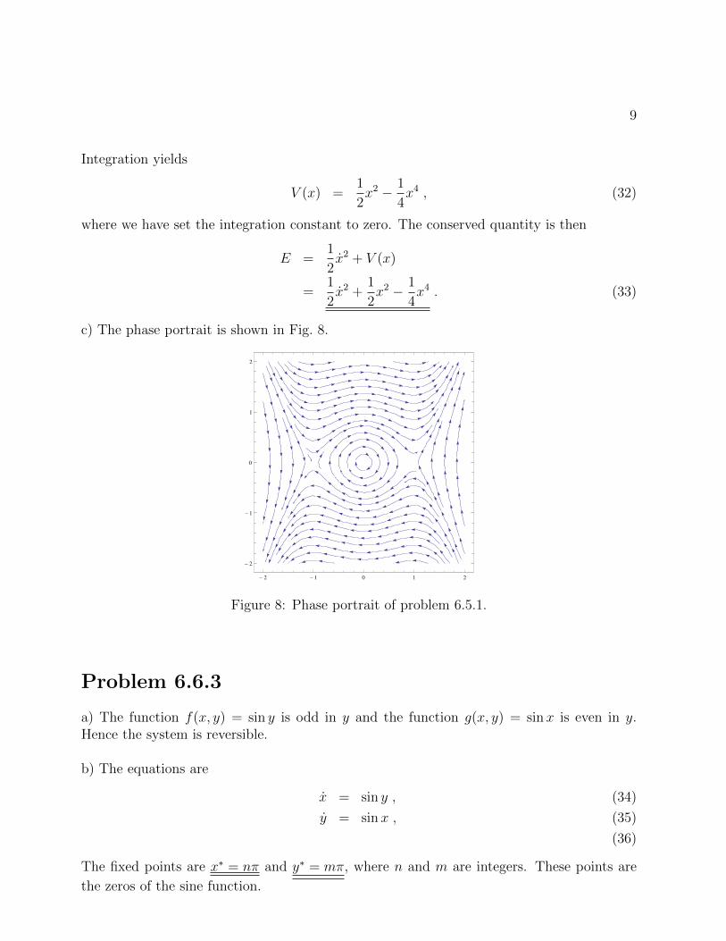
9

Integration yields

V (x) =1

2x2 − 1

4x4 , (32)

where we have set the integration constant to zero. The conserved quantity is then

E =1

2x2 + V (x)

=1

2x2 +

1

2x2 − 1

4x4 . (33)

c) The phase portrait is shown in Fig. 8.

- 2 -1 0 1 2

- 2

-1

0

1

2

Figure 8: Phase portrait of problem 6.5.1.

Problem 6.6.3

a) The function f(x, y) = sin y is odd in y and the function g(x, y) = sinx is even in y.Hence the system is reversible.

b) The equations are

x = sin y , (34)

y = sin x , (35)

(36)

The fixed points are x∗ = nπ and y∗ = mπ, where n and m are integers. These points are

the zeros of the sine function.

10

The Jacobian matrix is

A(x∗, y∗) =

(0 cos y∗

cos y∗ 0

), (37)

The eigenvalues are

λ1,2 = ±√

cosx∗ cos y∗ . (38)

cosnπ = 1 if n even and cosnπ = −1 if n odd. This implies that the eigenvalues areλ1,2 = ±1 if n and m are even or if n and m are odd. The fix point is then a saddle. If nis even and m odd or vice versa, the eigenvalues are λ = ±i. The fixed point is then a center.

c) We have

dy

dx=

y

x

=sinx

sin y. (39)

At a point on the line y = ±x , this ratio is ±1 and so vector field points along the lineitself. Hence, we stay on it.

d) The phase portrait and the type of fixed point can be seen in Fig. 9.

-4 -2 0 2 4

-4

-2

0

2

4

Figure 9: Phase portrait of problem 6.6.3.

11

Problem 6.6.10

The dynamics is given by the equations

x = −y − x2 , (40)

y = x . (41)

a) The only fixed point is the origin. The Jacobian matrix is given by

A(x, y) =

(0− 2x −1

1 0

). (42)

Evaluated at the origin, we find

A(0, 0) =

(0 −11 0

), (43)

and so the eigenvalues are λ = ±i. The origin is therefore a linear center. Note that thesystem in reversible since it is invariant under t → −t and y → −y. Theorem 6.6.1 thenapplies and the origin is a nonlinear center. The phase portrait is shown in Fig. 10.

-2 -1 0 1 2

-2

-1

0

1

2

Figure 10: Phase portrait of problem 6.6.10

Problem 6.7.1

The equation for the damped pendulum reads

θ + bθ + sin θ = 0 , (44)

12

where b > 0 is a parameter. Introducing ν = θ, we can write the above equation as

θ = ν , (45)

ν = −bν − sin θ . (46)

The fixed points are given by ν = θ = 0, i. e. ν = 0 and therefore sin θ = 0. The latteryields θ = 0 or θ = π. The fixed points are therefore (0, 0) and (π, 0). The Jacobian matrix

reads

A(θ, ν) =

(0 1

− cos θ −b

)(47)

This gives the characteristic equation for the eigenvalues

λ(λ+ b+ cos θ) = 0 . (48)

The solutions are

λ =−b±

√b2 − 4 cos θ

2. (49)

This yields τ = −b and ∆ = cos θ. For the fixed point (0, 0), this yields τ = −b and ∆ = 1.If τ 2 − 4∆ = b2 − 4 > 0, i.e. if b > 2, the fixed point is a stable node, and if b < 2, the fixedpoint is a stable spiral. Moreover, For the fixed point (0, π), this yields τ = −b and ∆ = −1.Thus the fixed point is a saddle point for all values of b.

Problem 7.1.4

The dynamics is governed by the equations

r = r sin r , (50)

θ = 1 . (51)

In Cartesian coordinates, this becomes

x = x sin√x2 + y2 − y , (52)

y = y sin√x2 + y2 + x . (53)

We note that θ = 1 everywhere and so the flow is always counterclockwise. The radial flowvanishes for r = π, 2π etc and so we have circular orbits for these values of r. Between thesevalues of r, the radial flow always has the same sign and it alternating. Between r = 0 andr = π, r > 0 and so flow is away from the origin. Between r = π and r = 2π, r < 0 and soflow is towards the origin. The circular orbits are therefore limit cycles and their stability isalternating.

The phase portrait is shown in Fig. 11.

13

-6 -4 -2 0 2 4 6

-6

-4

-2

0

2

4

6

Figure 11: Phase portrait of problem 7.1.4.

Problem 8.1.9

The equation for the anharmonic oscillator with damping reads 1

x+ bx− kx+ x3 = 0 . (54)

This can be written as

x = y , (55)

y = −by + kx− x3 . (56)

The fixed points are (0, 0) and (±√k, 0). The Jacobian matrix reads

A(x, y) =

(0 1

k − 3x2 −b

). (57)

This yields

A(0, 0) =

(0 1k −b

), (58)

and thus

λ =−b±

√b2 + 4k

2. (59)

1Note that we have damping for b > 0. For b < 0 we are pumping energy into the system. Also note thatthe linear force term is the usual if k < 0. For k > 0 the force is no longer restoring but pushes the particleaway from the origin. However, the cubic term stabilizes the system for all b and k.

14

Similarly

A(±√k, 0) =

(0 1−2k −b

), (60)

and thus

λ =−b±

√b2 − 8k

2. (61)

All fixed points are stable for b > 0 and unstable for b < 0. Whether it is a spiral or nodedepends on the sign of b2 + 4k and b2− 8k, respectively. For b = 0, there is no damping andthe system is conservative. The potential is V (x) = −1

2kx2 + 1

4x4. In this case, the origin is

stable for k < 0 and unstable for k > 0. The other fixed points only exist for k > 0 and theyare stable. This is the standard pitchfork bifurcation from chapter three. This is shown inFig. 12

Stable node

stable spiral

Stable spiral

Stable node

-3 -2 -1 0 1 2 3

-2.0

-1.5

-1.0

-0.5

0.0

0.5

1.0

b

k

Figure 12: Stability diagram. Everything to the left is unstable.

Problem 8.2.8

The equations governing the dynamics are

x = x[x(1− x)− y] , (62)

y = y(x− a) , (63)

where a ≥ 0 is a parameter.

a) The nullclines are given by x = 0 and y = 0 The former yields x = 0, and y = x(1− x),

while the latter gives y = 0 and x = a. This is shown Fig. 13 b) y = 0 gives y = 0 or x = a.

If y = 0, x = 0 implies that x = 0 or x = 1. If x = a x = 0 implies y = a(1 − a). Thusthe fixed points are (x, y) = (0, 0), (x, y) = (1, 0), and (x, y) = (a, a(1− a)). Note that last

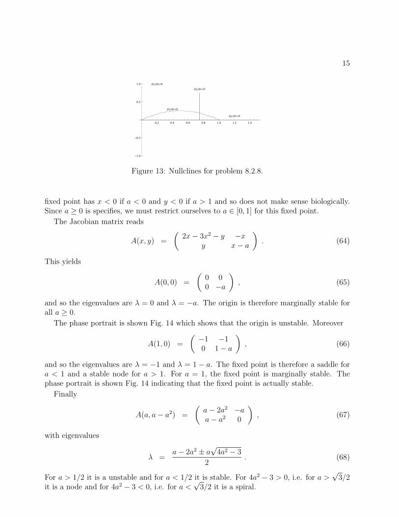
15

dx�dt=0

dx�dt=0

dy�dt=0

dy�dt=0

0.2 0.4 0.6 0.8 1.0 1.2 1.4

-1.0

-0.5

0.5

1.0

Figure 13: Nullclines for problem 8.2.8.

fixed point has x < 0 if a < 0 and y < 0 if a > 1 and so does not make sense biologically.Since a ≥ 0 is specifies, we must restrict ourselves to a ∈ [0, 1] for this fixed point.

The Jacobian matrix reads

A(x, y) =

(2x− 3x2 − y −x

y x− a

). (64)

This yields

A(0, 0) =

(0 00 −a

), (65)

and so the eigenvalues are λ = 0 and λ = −a. The origin is therefore marginally stable forall a ≥ 0.

The phase portrait is shown Fig. 14 which shows that the origin is unstable. Moreover

A(1, 0) =

(−1 −10 1− a

), (66)

and so the eigenvalues are λ = −1 and λ = 1− a. The fixed point is therefore a saddle fora < 1 and a stable node for a > 1. For a = 1, the fixed point is marginally stable. Thephase portrait is shown Fig. 14 indicating that the fixed point is actually stable.

Finally

A(a, a− a2) =

(a− 2a2 −aa− a2 0

), (67)

with eigenvalues

λ =a− 2a2 ± a

√4a2 − 3

2. (68)

For a > 1/2 it is a unstable and for a < 1/2 it is stable. For 4a2 − 3 > 0, i.e. for a >√

3/2it is a node and for 4a2 − 3 < 0, i.e. for a <

√3/2 it is a spiral.

16

0.0 0.5 1.0 1.5

0.0

0.2

0.4

0.6

0.8

1.0

Figure 14: Phase portrait for a = 1 in problem 8.2.8.

c) The phase portrait is shown Fig. 15 which shows that you will flow to the line y = 0,i.e. the predators will go extinct. d) We have seen that the real part of the eigenvalues gothrough a zero at a = ac = 1/2. Thus we have a Hopf bifurcation. The fixed point is losingstability and after that it is surrounded by a stable limit cycle (going towards lower valuesof a). It is therefore supercritical. The phase portrait for a = 1/2 is shown in Fig. 16. e)Fora = 1/2, the imaginary part of the eigenvalue is ω =

√2/4.

f)

Problem 10.1.9

The map is

xn+1 =2xn

1 + xn. (69)

The fixed points x are given by the equation

x =2x

1 + x. (70)

This yields

x2 + x = 2x , (71)

or x = 0 and x = 1. The stability is given by the derivative of the function f(x) = 2x/(1+x):

f ′(x) =2

(1 + x)2. (72)

17

0.0 0.5 1.0 1.5

0.0

0.2

0.4

0.6

0.8

1.0

Figure 15: Phase portrait for a = 2 in problem 8.2.8.

This yields f ′(0) = 2 and f ′(1) = 12. Hence the fixed point x = 0 is unstable and the fixed

point x = 1 is stable.

Problem 10.1.10

The map is

xn+1 = 1 +1

2sin(xn) . (73)

In Fig 17, we show the functions g(x) = x and h(x) = 1 + 12

sinx from which it is evidentthat there is a unique fixed point that corresponds to the intersection of the curves.

The derivative of the function f(x) = 1 + 12

sinx is is

f ′(x) =1

2cosx . (74)

Since |f ′(x)| ≤ 12, the fixed point is stable.

Problem 10.1.12

Consider the map

f(xn) = xn −g(xn)

g′(xn). (75)

18

0.0 0.5 1.0 1.5

0.0

0.2

0.4

0.6

0.8

1.0

Figure 16: Phase portrait for a = 1/2 in problem 8.2.8.

-3 -2 -1 1 2 3x_n

-3

-2

-1

1

2

3

x_8n+1<

Figure 17: Fixed point of the map xn+1 = 1 + 12

sin(xn).

a) For the function g(x) = x2 − 4, this yields

f(xn) = xn −x2n − 4

2xn. (76)

b) The fixed points are given by

x = x− x2 − 4

2x. (77)

This yields x2 − 4 = 0 or x = ±2.

c) The derivative is

f ′(x) =1

2− 2

x2, (78)

19

and so

f ′(±2) = 0 . (79)

This shows that the fixed points are supestable.

d) Try it out!

Problem 10.1.13

Differentiation of f(x) gives

f ′(x) =g(x)g′′(x)

[g′(x)]2. (80)

Unless g′(x) = 0, g(x) = 0 corresponds to f ′(x) = 0, i.e. a zero of g(x) corresponds to asuperstable fixed point for f(x).

Problem 10.3.11

The map is given by

xn+1 = −(r + 1)x− x2 − 2x3 . (81)

a) Clearly x = 0 is fixed point. It stability is determined by the derivative of f(x) =−(r + 1)x− x2 − 2x3:

f ′(x) = −(r + 1)− 2x− 6x2 . (82)

This yields f ′(0) = −1− r and so the origin is stable for −2 < r < 0.

b) We notice that f ′(0) = −1 for r = 0, which is the criterion for a flip bifurcation.

c) The period-2 cycles satisfy f(f(x)) − x = 0. Since f(x) − x is a factor in this poly-nomial, we obtain by long division

[−(2 + r)x− x2 − 2x3][−r + rx− (1 + 2r + 2r2)x2 − 4rx3 − 2(3 + 4r)x4 − 8x5 − 8x6] = 0 .

(83)

We are interested in a bifurcation for small negative values of r around x = 0. We can thenapproximate the second polynomial with

−r + rx− x2 = 0 , (84)

20

whose solutions are x = (r ±√r2 − 4r)/2 ≈= ±

√−r. Thus the cycle exists for r < 0

and coalesces with x = 0 as r → 0−. The stability is determined by the derivative off(f(x)) evaluated at the points of the cycle, i. e. by the chain rule f ′(

√−r)f ′(−

√−r) ≈

(−1− 2√−r)(−1 + 2

√−r) = 1− 4r > 1 and the 2-cycle is therefore unstable.

d) Use a cobweb to show that x → 0 for |x| small and r < 0 and x → ∞ for |x| smalland r > 0.

Problem 10.4.2

The map is given by

xn+1 =rx2n

1 + x2n. (85)

The origin is always a fixed point. The other fixed points are given by x2 − rx+ 1, or

x± =r ±√r2 − 4

2. (86)

These fixed points exist for r ≥ 2. Moreover

f ′(x) =2rx

(1 + x2)2, (87)

which shows that the origin is always stable. At r = 2, the new fixed point is x = 1 and sof ′(1) = 1. This shows that bifurcation is a tangent bifurcation. At the fixed point x±, wehave

f ′(x±) =2

1 + x2, (88)

which is always larger than zero. Thus there is no period-doubling. We can also prove thisexplicitly for a period-2 cycle. The existence of such a cycle implies f [f(x)] = x. Since thesolutions to f(x) = x are also solutions to f [f(x)] = x, we can use long division to writef [f(x)] = x as

[(1 + x2)(1 + x(r + x+ r2x))]

[1 + 2x2 + (1 + r2)x4)]. = 0 . (89)

The first term in the numerator has no solution. The second term yields (r2+1)x2−rx+1 = 0,which gives

x = −r ±

√r2 − 4(r2 + 1)

2(1 + r2). (90)

which has no real solution, as anticipated. No chaos and no intermittency.

21

Problem 10.4.3

The map is given by

xn+1 = 1− rx2n . (91)

A superstable n-cycle has by definition [fn(x)]′ = 0. Using the chain rule, this is equivalentto f ′(x) = 0. In the present case, we have f(x) = 1− rx2 and so f ′(x) = 0 yields −2rx = 0,i.e. x = 0. Moreover

f 3(x) = 1− r[1− r(1− rx2)2]2 . (92)

The 3-cycle satisfies f 3(x) = x, where x = 0 is in the cycle. Inserting x = 0 into f 3(x) = xgives

1− r(1− r)2 = 0 , (93)

which is the sought polynomial.

Problem 10.5.4

The Lyapunov exponent is λ = log r and so chaos exists for r > 1. This implies there canbe no periodic window 1 < r1 < r < r2 after the onset of chaos.

Problem 10.7.6

Since R2 is defined by superstability of the 4-cycle, we know that x = 0 is a point on thatcycle. Thus f 4(0, R2) = 0. This yields a polynomial for R2:

R2 −R22 + 2R3

2 − 5R42 + 6R5

2 − 6R62 + 4R7

2 −R82 = 0 . (94)

Since R2−R22 is a factor of the above polynomial (since R2−R2

2 = 0 defines the superstable2-cycle), we find

1 +R22(R2 − 2)(R2 − 1)(1 +R2

2) = 0 . (95)

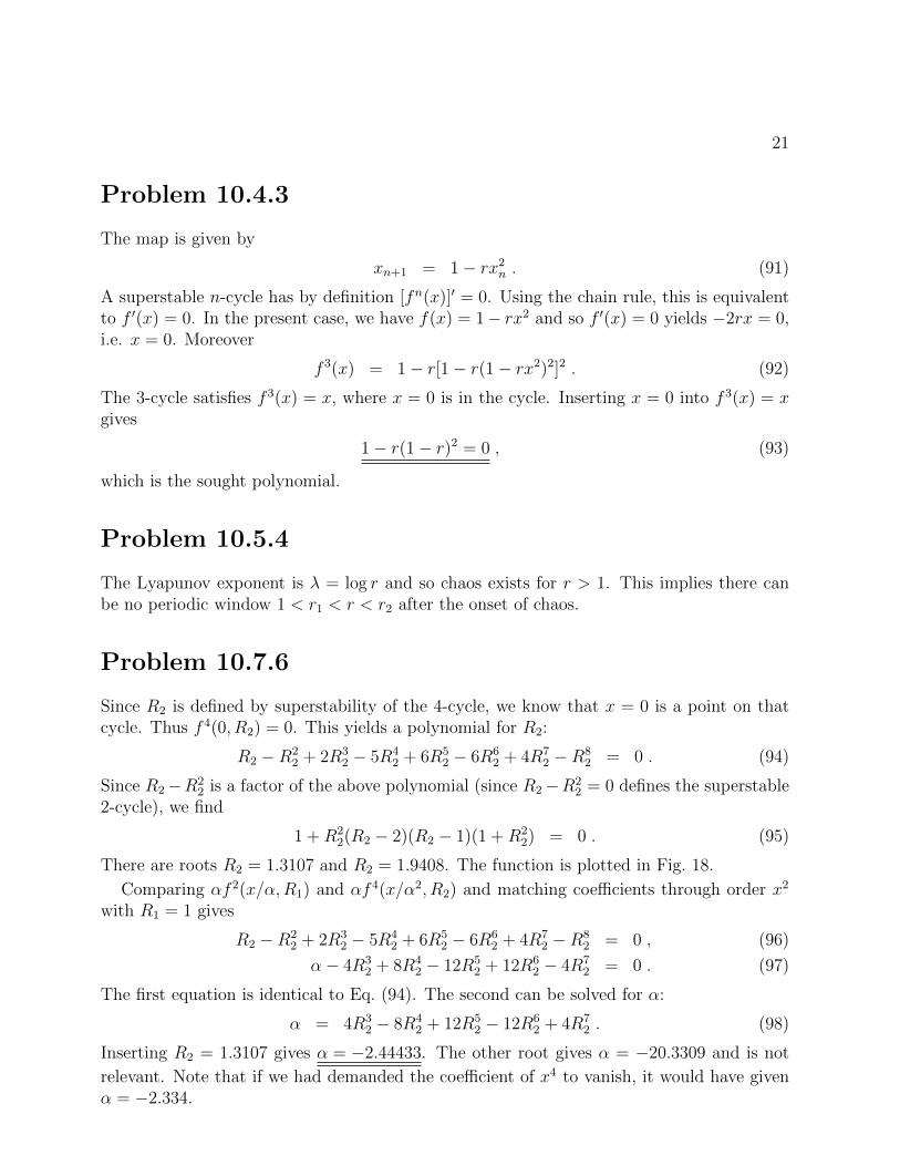
There are roots R2 = 1.3107 and R2 = 1.9408. The function is plotted in Fig. 18.

Comparing αf 2(x/α,R1) and αf 4(x/α2, R2) and matching coefficients through order x2

with R1 = 1 gives

R2 −R22 + 2R3

2 − 5R42 + 6R5

2 − 6R62 + 4R7

2 −R82 = 0 , (96)

α− 4R32 + 8R4

2 − 12R52 + 12R6

2 − 4R72 = 0 . (97)

The first equation is identical to Eq. (94). The second can be solved for α:

α = 4R32 − 8R4

2 + 12R52 − 12R6

2 + 4R72 . (98)

Inserting R2 = 1.3107 gives α = −2.44433. The other root gives α = −20.3309 and is not

relevant. Note that if we had demanded the coefficient of x4 to vanish, it would have givenα = −2.334.

22

0.5 1.0 1.5 2.0r

-1.0

-0.5

0.5

1.0

fHrL

Figure 18: Polynomial for R2.

Problem 11.1.6

The decimal shift map is given by

xn+1 = 10xn (mod 1) . (99)

The map is shown is Fig. 19.

0.2 0.4 0.6 0.8 1.0x_n

0.02

0.04

0.06

0.08

0.10

x_8n+1<

Figure 19: Decimal shift map.

a) A rational number y can be represented in decimal form

y = x0.x1x2x3.. , (100)

where either the sequence of numbers is finite or it is periodic. If yo ∈ Q, then we willeventually end up at y = 0 if the sequence is finite, or a periodic orbit given by the period-icity of the decimal representation. Thus a rational corresponds to a periodic orbit and Qis countable. Since the derivative of the decimal shift map is 10 (see Fig. 19), every orbit is

23

unstable.

b) A irrational number has a aperiodic decimal representation and so if y0 ∈ R\Q willgive rise to an aperiodic orbit. The irrational numbers are uncountable.

c) A number on the form x0 = c1c2....cNcN ..., will after n = N iterations be mapped toxn = cNcN ..... After n+ 1 iterations we also have xn+1 = cN ... and so it is fixed point. Sucha number will be periodic and therefore x0 ∈ Q. The set is thus countable.

Problem 12.1.1

If either |a| > 1 or |b| > 1, the sequence {(xn, yn)} will wander off to infinity. If |a| = |b| = 1,any (x0, y0) is a fixed point. If |a| < 1 and |b| < 1, the sequence {(xn, yn)} converges to theorigin. The way the sequence approaches the origin depends on the sign of a and b and inwhich quadrant you start i. e. of the point (x0, y0). For example if 0 < a1 < and −1 < b < 0and (x0, y0) is in the first quadrant, the sequence will hop between the first and the thirdquadrant. Likewise if 0 < a < 1 and −1 < b < 0 and (x0, y0) is in the second quadrant, thesequence hops between the second and third quadrant. The other cases, can be treated inthe same way.

Problem 12.1.5

a) We can write (x0, y0) as (.a1a2a3..., .b1b2b3...), where ai and bi are either 0 or 1. If x0 <12,

then a1 = 0 and x0 is multplied by two which corresponds to moving all digits one place tothe left. Thus x1 = .a2a3.... Then y0 is multiplied by a 1

2which corresponds to moving all

digits one place to the right. This implies that B(x, y) = (.a2a3...0b2b3...) If x0 ≥ 12, then

a1 = 1. Multiplying by 2 and subtracting by one corresponds to moving all digits to theleft and dropping a1. Thus x1 = .a2a3.... Now y0 is multiplied by a 1

2and we add 1

2The

first operation is again moving all digits to the right while the second implies that the firstdigit will be one (since 1

2=0.1in the binary representation). Since a1 = 1 we can write this

as y = .1b2b3... = .a1b2b3... and so in both case we can write B(x, y) = (.a2a3...a1b2b3...).

b) The only possibility for a period-2 orbit is that x = 0.101010... or x = 0.01010... since Bmoves the all digits to the left and B2(x, y) = (x, y). After two iteration of y0, we know thatb1b2 has been replaced by a2a1 and so y = 0.010101 is the only possibility for x = 0.101010...and vice versa (use the same argument to determine b3...). The number x = 0.101010...equals

x =1

2+

1

23+ ...

=2

3. (101)

24

Likewise, you can show that x = 0.010101... = 13.

c) The only periodic orbits must be rational numbers because these numbers are eitherfinite or periodic in the decimal representation and the action on x is to move all the digitsto the left. y must also be rational, otherwise (x, y) cannot be periodic. In addition thereare additional requirements analogous to those derived in b); b1 = an, b2 = an−1 etc for ann-cycle. Since the cartesian product Q×Q is countable, it follows.

d) Pick x irrational and y anything. x irrational implies that the orbit cannot be peri-odic since the action on x is to move all the digits to the left. Since the irrationals areuncoutable the results follows.