thaís machado de matos vilela three essays on gasoline and ... · three essays on gasoline and...
TRANSCRIPT
Thaís Machado de Matos Vilela
Three essays on gasoline and automobile markets in Brazil
Tese de Doutorado
Thesis presented to the Programa de Pós-Graduação em Economia of the Departamento de Economia da PUC-Rio, as partial fulfillment of the requirements for the degree of Doutor.
Advisor: Prof. Leonardo Bandeira Rezende
Rio de Janeiro
March 2015

Thaís Machado de Matos Vilela
Three essays on gasoline and automobile markets in Brazil
Thesis presented to the Programa de Pós-Graduação em Economia of the Departamento de Economia da PUC-Rio, as partial fulfillment of the requirements for the degree of Doutor.
Prof. Leonardo Bandeira Rezende Advisor
Departamento de Economia – PUC-Rio
Prof. Marcelo Cunha Medeiros Departamento de Economia – PUC-Rio
Prof. Juliano Junqueira Assunção Departamento de Economia – PUC-Rio
Prof. Helder Queiroz Pinto Jr. Instituto de Economia - UFRJ
Prof. Cláudio Ribeiro de Lucinda Faculdade de Economia, Administração e Contabilidade, RP - USP
Rio de Janeiro, March 26th, 2015

All rights reserved.
Thaís Machado de Matos Vilela
The author graduated in Economics from Fundação
Getúlio Vargas – EPGE – in 2005. She obtained the
degree of Mestre em Economia at Universidade Federal
do Rio de Janeiro in 2009.
Bibliographic Data
CDD: 330
Vilela, Thaís Machado de Matos
Three essays on gasoline and automobile
markets in Brazil / Thaís Machado de Matos Vilela ;
advisor: Leonardo Bandeira Rezende. – 2015.
113 f. : il. (color.) ; 30 cm
Tese (doutorado) – Pontifícia Universidade
Católica do Rio de Janeiro, Departamento de
Economia, 2015.
Inclui bibliografia
1. Economia – Teses. 2. Gasolina. 3. Álcool
combustível. 4. Flex-fuel 5. Cointegração. 6.
Variáveis instrumentais. 7. Automóvel. 8. BLP. 9.
Política de preços. 10. Emissões de CO2. I.
Rezende, Leonardo Bandeira. II. Pontifícia
Universidade Católica do Rio de Janeiro.
Departamento de Economia. III. Título.

Acknowledgements
I would like to thank my advisor, Professor Leonardo Bandeira Rezende, for all
the fruitful discussions. I appreciate his contribution of time and ideas and, most
important, his support during the process of writing my PhD thesis.
To my thesis committee – Prof. Marcelo Medeiros, Prof. Juliano Assunção, Prof.
Helder Queiroz, and Prof. Caludio Lucinda – I would like to thank for your
comments and suggestions during the PhD defense. A special thanks to Prof.
Medeiros, who helped me with the first chapter of this thesis.
Also, I want to thank CNPq and CAPES for the funding support. The funding
from CAPES allowed me to be a Visiting Student Researcher at the University of
California, Berkeley, for five months. While at the Department of Agriculture and
Resource Economics in Berkeley, I had the opportunity to attend seminars and
discuss my research with leading researchers in the field. Because of this unique
experience I was able to talk several times to Professor Lucas Davis, whose paper
about the cost of fuel subsidies inspired me to write the third chapter of this thesis.
I also thank Professor Meredith Fowlie for being my sponsor while at UC,
Berkeley.
To the Department of Economics staff I would like to express my deeply
appreciation for the support given me during the almost five years. Also, a special
thanks to my friends and colleagues that made my time at PUC certainly more
enjoyable
Finally, I would like to thank and dedicate this PhD thesis to my family. They
gave me the encouragement to continue pursuing this path. A special thanks to my
parents, brother and husband. I cannot thank them enough for helping me through
the hard times.

Abstract
Vilela, Thaís Machado de Matos; Rezende, Leonardo Bandeira (advisor).
Three essays on gasoline and automobile markets in Brazil. Rio de
Janeiro, 2015. 113 p. PhD Thesis – Departamento de Economia, Pontifícia
Universidade Católica do Rio de Janeiro.
This thesis is comprised of three independent chapters about gasoline and
automobile markets in Brazil. In the first two chapters we are interested in the
relationship between consumers’ behavior and the flex-fuel technology. In the
first chapter, we focus on how sensitive Brazilian consumers are to fuel price
changes, especially after the introduction of the flex-fuel technology on March
2003. We estimate the own- and cross-price elasticities of gasoline demand taking
into account fuel prices endogeneity. We combine two identification strategies –
Dynamic Ordinary Least Square and Instrumental Variables. Our results present
evidences that the introduction of the flex-fuel technology changed consumers’
perception regarding fuel prices fluctuations: consumers became more elastic
regarding both gasoline and ethanol after the introduction of the new technology.
In the second chapter, we focus on the automotive market. We measure the
importance of the flex-fuel technology for consumers when buying a new
automobile and we attempt to, through a detailed descriptive analysis, shed some
light on the process of introduction of this new automobile characteristic in Brazil.
Using only aggregate data, we follow the BLP (1995) approach: we use a discrete-
choice model with random coefficients to estimate the demand and the supply
parameters. To control for the price endogeneity in the demand curve, we use
linear combinations of the automobile characteristics (except for the price) as
instruments. The results suggest that the flex-fuel technology is not an important
attribute when all the other automobile characteristics are controlled for. This
result suggests that the rapid growth in sales is mostly explained by the supply
side: automakers’ decision to offer only flex-fuel for any other reasons not
associated with demand. Finally, in the third chapter, we calculate the economic
and environmental costs of government intervention in the gasoline market
through its majority position in Petrobras. Based on Microeconomic Theory, we
calculate that the deadweight loss resulting from this policy equaled R$ 17 billion

from January 2002 to January 2013. When considering separately the effects of
this intervention on the emissions of CO2, on the ethanol market and on the
inflation rate, we find that the economic cost increases substantially.
Keywords
Gasoline; ethanol; flex-fuel; cointegration; Instrumental Variables;
automobile; BLP; pricing policy; CO2 emissions.
Resumo
Vilela, Thaís Machado de Matos; Rezende, Leonardo Bandeira
(orientador). Three essays on gasoline and automobile markets in
Brazil. Rio de Janeiro, 2015. 113 p. Tese de Doutorado – Departamento
de Economia, Pontifícia Universidade Católica do Rio de Janeiro.
Esta tese é composta de três capítulos independentes sobre os mercados de
gasolina e de automóveis no Brasil. Nos dois primeiros capítulos, estamos
interessados na relação entre o comportamento do consumidor e a tecnologia flex-
fuel. No primeiro capítulo, analisamos como a introdução da tecnologia flex-fuel a
partir de 2003 mudou as elasticidades-preço própria e cruzada da demanda por
gasolina no Brasil. Para calcular as elasticidades, combinamos duas estratégias de
identificação: Mínimos Quadrados Ordinários Dinâmicos e Variáveis
Instrumentais. Os resultados sugerem consumidores mais elásticos às mudanças
nos preços dos combustíveis do que estudos anteriores, sugerindo que a
introdução da tecnologia flex-fuel mudou o comportamento do consumidor. No
segundo capítulo, estudamos o mercado automotivo. Procuramos entender como
se deu o processo de introdução da tecnologia flex-fuel e estimamos a importância
dessa nova tecnologia para o consumidor. Para tanto, usamos a metodologia
proposta em BLP (1995): um modelo de escolha discreta com coeficientes
aleatórios para estimar os parâmetros da demanda por e da oferta de automóveis.
Para corrigir a endogeneidade dos preços na curva de demanda, usamos
combinações lineares das características dos automóveis (exceto preço) como
instrumentos. Os resultados sugerem que a tecnologia flex-fuel não é valorizada
pelos consumidores quando outras características são controladas. Este resultado
sugere que o rápido crescimento das vendas dos automóveis flex-fuel pode ser
mais bem explicado pelo lado da oferta. Finalmente, no terceiro capítulo,
calculamos os custos econômicos e ambientais da intervenção do Governo Federal
através de sua posição majoritária na Petrobras. Com base na Teoria
Microeconômica, calculamos o peso morto gerado por tal política governamental.
Encontramos um custo total de R$ 17 bilhões entre janeiro de 2002 e janeiro de
2013. Ao analisarmos separadamente os impactos ambientais – emissões de CO2 –
e os efeitos sobre o consumo de álcool hidratado e sobre a inflação, verificamos
que o custo econômico aumenta substancialmente.

Palavras-chave
Gasolina; álcool combustível; flex-fuel; cointegração; Variáveis
Instrumentais; automóvel; BLP; política de preços; emissões de CO2.

Contents
1 Did flex-fuel technology change the price elasticities of fuel consumption? A new approach for estimating gasoline demand in Brazil
12
1.1 Introduction 12 1.2 Price elasticities in other empirical studies 14 1.3 Data 17 1.4 Methodology 22 1.5 Results 28 1.6 Additional Robustness Checks 33 1.7 Conclusion 39
2 Does flex-fuel technology matter for automobile demand? A structural analysis using a random coefficients discrete choice model
41
2.1 Introduction 41 2.2 Discrete choice models and the automobile industry 43 2.3 Data 46 2.4 Model 60 2.5 Results 68 2.6 Conclusion 78 2.7 Appendix A2 80
3 The economic cost of government intervention in the gasoline market: a case study from Brazil
82
3.1 Introduction 82 3.2 Data 84 3.3 Income transfer from distorted gasoline prices 88 3.4 Efficiency losses caused by gasoline price distortion 90 3.5 Price stability and CO2 emissions 97 3.6 The effects of price stability on the consumption of ethanol 99 3.7 Conclusion 101 3.7 Appendix A3 102
4 References 107

List of Tables
Table 1.1: Database description 19
Table 1.2: Annual GDP variation and gasoline consumption variation 21
Table 1.3: First-stage results: OLS estimates of TRS price on
ethanol price
29
Table 1.4: Second-stage results: DOLS and IV estimates of fuel
prices on gasoline demand
30
Table 1.5: Second-stage results: DOLS and IV estimates of fuel
prices on gasoline demand for different time periods
32
Table 1.6: The elasticity of gasoline demand using different income
proxies
35
Table 1.7: The elasticity of gasoline demand using different identification strategies
36
Table 1.8: Fuel price elasticities of gasoline demand including
natural gas as a fuel alternative
39
Table 2.1: Ratio between our sample and ANFAVEA’s data (%) 47
Table 2.2: Share of flex-fuel in total sales of new automobiles (%) 48
Table 2.3: Descriptive statistics - average between models per year 54
Table 2.4: Descriptive statistics by fuel type (cont.) 57
Table 2.5: Hedonic price model results 59
Table 2.6: OLS and IV demand estimations 71
Table 2.7: Estimated demand parameters using the random
coefficient model (BLP specification, 870 observations)
73
Table 2.8: Estimated demand parameters using the random
coefficient model and income dummies (BLP specification, 870
observations)
75
Table 2.9: OLS supply estimation of marginal cost on product
characteristics
78
Table A2.1: Estimated demand parameters using the random
coefficient model and income dummies (simplified BLP specification,
870 observations)
81
Table 3.1: Deadweight loss from the gasoline price stability policy in
Brazil
95

List of Figures
Figure 1.1: New automobile licensing by fuel type 13
Figure 1.2: Fuel consumption in Brazil 20
Figure 1.3: Relative consumption and relative price (%) 22
Figure 1.4: Gasoline demand response to transitory shocks in the
gasoline supply (Panel A) and in the ethanol market (Panel B)
33
Figure 1.5: Gasoline demand response to transitory shocks in the
gasoline supply (Panel A) and in the ethanol market (Panel B) - without
CIDE as instrument=
37
Figure 2.1: Ratio between the price of ethanol and the price of gasoline 50
Figure 2.2: Gol Power 1.6 - the first automobile with the flex-fuel
technology sold in Brazil
51
Figure 2.3: Market-shares by fuel type 52
Figure 2.4: Share of flex-fuel automobiles relative to total automobile
sales - by model
55
Figure 2.5: Ratio between the price of flex-fuel automobiles and the
price of gasoline engine automobiles
55
Figure 2.6: Descriptive statistics by fuel type 56
Figure 2.7: Automobile production in Brazil (in units) 58
Figure 2.8: Own-price elasticity of new automobile demand from the
logit and the full models
75
Figure 3.1: Gasoline price in the international market and the
wholesale gasoline price in Brazil
86
Figure 3.2: Inflation target 86
Figure 3.3: Gasoline consumption in Brazil (in liters) 87
Figure 3.4: Ratio between the prices of ethanol and gasoline 88
Figure 3.5: Income transfer resulting from the gasoline price policy 89
Figure 3.6: The economic cost of gasoline price policy 92
Figure 3.7: Gasoline consumption (in liters) 94
Figure 3.8: CO2 emissions resulting from the gasoline pricing policy in Brazil
98
Figure 3.9: Ethanol consumption under the baseline and the alternative
scenarios (in liters)
100
Figure A3.1: Response of the inflation rate to a one-standard deviation
shock in the price of gasoline with two standard error bounds
106

1
Did flex-fuel technology change the price elasticities of fuel
consumption? A new approach for estimating gasoline
demand in Brazil
1.1
Introduction
Since March 2003, automakers in Brazil produce automobiles designed to
run on gasoline, ethanol or any mixture of both fuels. The well-developed1 ethanol
distribution network in Brazil allows consumers to find gasoline and ethanol in
any filling station, allowing them to choose between both fuels according to fuel
prices and their preferences. Understanding how consumers respond to changes in
prices of both fuels is important for developing and evaluating energy and
environmental policies, and for decreasing the unpredictability of fuel demand for
producers.
In this chapter, we answer the following question: did flex-fuel technology
change the long run own- and cross-price elasticities of gasoline demand? There is
a widely-accepted standpoint that the introduction of the flex-fuel technology
represented a structural change in the gasoline markets, and that the price of
ethanol became an important variable to explain changes in the demand for
gasoline (ANP, 2013). By estimating the own- and cross-price elasticities for
different periods and comparing the results we are able to test both hypotheses.
As shown in Figure 1.1, flex-fuel automobiles represented over 90 percent
of total sales only four years after the introduction of the new technology. To
estimate the impact of the flex-fuel technology in the gasoline market, we divide
our sample into two equal time periods. We interpret the period from December
2002 to December 2007 as the introduction phase and the one from January 2008
to January 2013 as the consolidation phase. Ideally, one would use more data from
the period before the introduction of the new technology, but data before
December 2002 is unavailable for some key variables. This limitation can
1 All gas stations in Brazil sell gasoline and ethanol.

13
possibly mean that the results are lower bounds on the effect of the new
technology, since flex-fuel automobiles already compose part of the fleet in the
first period.
Figure 1.1 New automobile licensing by fuel type
Source: Anfavea, statistical yearbook 2014.
We follow the Engle and Granger Two-Step procedure to estimate long
run elasticities and shorter-term dynamics. The first step is the identification of the
long run demand for gasoline. Different from most papers in the demand for fuel
literature, especially those which use Brazilian data, we take into account that
gasoline and ethanol are potential endogenous variables in the gasoline demand
and supply equations. To correctly identify the estimated equation as a demand
equation, we rely on two different identification strategies. Endogeneity in the
non-stationary variables is controlled using Dynamic Ordinary Least Squares
(DOLS), while an Instrumental Variables (IV) approach is used for the others.
In the second step of the Engle and Granger procedure, we go one step
further from what is commonly done in the fuel demand literature and calculate
the response of gasoline demand to shocks in the prices of gasoline and ethanol.
To estimate the Impulse Response Functions (IRF), we use a non-recursive
identification strategy to be sure that we are estimating the parameters of the

14
demand equation. We impose some restrictions on the contemporaneous
relationships between the variables in our model, while also including another
instrument for gasoline demand based on Brazilian regulation.
We have four main results. First, controlling for price endogeneity matters.
Consistent with the endogeneity hypothesis, we find higher long run own- and
cross-price elasticities of gasoline demand (in absolute values) than previous
papers. Second, the own price elasticity increases in absolute value from the initial
period to the final one. Third, the long run cross-price elasticity of gasoline
demand in the consolidation period is substantially higher than and statistically
different from the cross-price elasticity found for the introduction period. These
shifts in consumers’ behavior corroborates with the view that the introduction of
the flex-fuel technology represented an important change in the gasoline market.
Fourth, in the second step of the Engle and Granger procedure, we find that
transitory shocks in the prices of gasoline and ethanol lead to permanent changes
in the demand for gasoline.
The remainder of this chapter is organized as follows. Section 1.2 sets the
background by describing previous studies that estimate price elasticity of
gasoline demand. Section 1.3 describes the data. Section 1.4 presents the model
and the identification strategy. Sections 1.5 and 1.6 presents the results and
additional robustness checks, respectively. Section 1.7 concludes the chapter.
1.2
Price elasticities in other empirical studies
Since the first crude oil shock, in 1973, there has been a growing literature
on automobile fuel market. Most studies are interested in the demand-side fuel
market and most have been done using United States data. Although many studies
differ methodologically, the main controversial aspect concerns the exogeneity
hypothesis about fuel prices.
Almost all papers assume that fuel prices are exogenous variables in the
fuel demand equation. There is a well-accepted standpoint that fuel prices –
mainly, gasoline price – are largely determined by the international crude oil
price. This hypothesis, however, may be too strong, and ignoring the potential fuel

15
price endogeneity may leads to estimates that are downward bias. To control for
fuel price endogeneity, the identification strategy most used is IV. Finding valid
and strong instruments for fuel prices, however, has been a challenge.
Ramsey et al (1975) and Dahl (1979) use the price of other crude oil-
related products, such as kerosene and heavy fuel oil, as instrument for the price
of gasoline in the United States. However, it is likely that these prices are
correlated with gasoline demand shocks via shocks in the international crude oil
market. If this is true, then the orthogonality condition is not satisfied and both
prices are not valid as instruments for the price of gasoline.
In Yatchew and No (2001) and Manzan and Zerom (2008), regional
dummies are used as instruments for the price of gasoline. However, if the
regional dummies are capturing, for example, the level of development in each
state, then the dummies are probably correlated with the gasoline demand within
that state. In this case, the exclusion restriction is violated.
Burke and Nishitateno (2011), Scott (2012) and Coyle et al (2012) use,
respectively, proven crude oil reserves, disruptions in crude oil production and the
crude oil price in the international crude oil market as instruments for the price of
gasoline. The validity of each variable as instrument depends on its non-
correlation with gasoline demand shocks.
In an attempt to find better instruments, Scott (2012) also uses federal and
state gasoline taxes (excluding ad valorem taxes) as instruments for the price of
gasoline. According to the author, tax level is a major source of price variation in
both time and state dimensions in the United States and it should not be gasoline
demand-driven.
Instead of using the gasoline taxes level, Davis and Killian (2011) use
inflation-adjusted change in the log of the tax per gallon as instrument for the
price of gasoline. The hypothesis is that even though tax legislation may respond
to current prices, the implementation of tax changes typically occurs with a lag,
making it reasonable to believe that changes in tax rates are uncorrelated with
unobserved changes in the demand for gasoline in the United States.
In the search of a stronger instrument for the gasoline price in the United
States, Liu (2011) argues that if almost all variation in the price of gasoline is
explained by changes in the international crude oil market, then the price of
gasoline across the states must be correlated. Therefore, Liu (2011) uses the

16
average gasoline price by state – excluding the adjacent states – as instrument for
the price of gasoline in each state. Once more, the validity of this identification
strategy depends on the non-correlation among the gasoline demand shocks in
each state.
Liu (2011) finds similar results for gasoline price elasticity estimates when
ignoring price endogeneity. Different from other papers, Liu (2011) argues that
the gasoline price is endogenous only to a minor extent and, therefore, the bias
size could be ignored.
With less ambiguity, most papers in the demand for fuel literature that use
Brazilian data assume that fuel prices are exogenous variables in the fuel demand
equation. There is a widely accepted standpoint that fuel prices in Brazil are
determined by the federal government and do not respond to changes in the fuel
market conditions – or if it does, it is to a minor extent.
Because of several changes in the Brazilian fuel market from 1975 to
2003, the estimates of fuel prices elasticities differ considerably from one study to
another. Overall, almost all papers that use more recent data set indicate that
since the introduction of the flex-fuel technology on March 2003, consumers’
sensitivity to fuel prices variation has changed (Nappo (2007), Silva et al (2009)
and Santos (2013)).
Nappo (2007) explicitly estimates the effect of the flex-fuel technology in
the long run price elasticities of gasoline demand in Brazil. To capture the change
in consumers’ response to fuel prices variation, Nappo (2007) uses an interaction
between a dummy variable – equal to 1 after March 2003 and 0 otherwise – and
the gasoline price. According to Nappo (2007), because of the presence of
multicollinearity between gasoline and ethanol prices, ethanol price is excluded
from the main regression equation.2
Taking out the ethanol price from the model, however, introduces an
omitted variable bias. Ethanol price is positively correlated with gasoline demand
and with the other independent variables. Thus, the omission of the ethanol price
introduces an upward bias in Nappo (2007). On the other hand, as with other
studies, Nappo (2007) does not take into account fuel prices endogeneity, leading
2 We find that the correlation between the price of gasoline and the price of ethanol is 0.49. We use
the state-level average price (inflation adjusted) for Brazil to calculate this correlation. As there is
no perfect (or close to perfect) collinearity, we do not exclude the price of ethanol from our
regressions

17
to a downward bias. Thus, in this case, it is hard to determine the final direction of
the bias.
As with Nappo (2007), our interest lies in the probable consumers’
behavior change after the introduction of the flex-fuel automobiles in Brazil.
However, to obtain better estimates of the long run own- and cross-price
elasticities of gasoline demand, we take into account the potential fuel price
endogeneity in the gasoline demand curve. We have no knowledge of a study that,
using Brazilian data, controls for both gasoline and ethanol prices endogeneity.
Within this context, this paper contributes to the literature by developing a
new identification strategy. We combine a cointegration technique – DOLS – and
IV approach to control for fuel prices endogeneity. Also, in the second stage of
Engle and Granger’s methodology, we estimate a full system error correction
model instead of a single-equation model, which is more common in the demand
for fuel literature. To identify the error correction model, we use a non-recursive
strategy. This approach allows us to draw IRF to assess the relevance of shocks in
the prices of gasoline and ethanol on the gasoline market.
1.3
Data
1.3.1
Data set
In this study, we use data from different sources. From the National
Petroleum, Natural Gas and Biofuel Agency (ANP, acronym in Portuguese), we
get data on gasoline consumption and on gasoline and ethanol prices sold in filling
stations over different Brazilian states. ANP provides state-level averages of both
consumption and price data. To get constant prices, we use the official Extended
Consumer Price Index (IPCA) from the Brazilian Institute of Geography and
Statistics (IBGE). Prices are converted to January 2013 Brazilian Reais.
From the National Traffic Department (DENATRAN), we get data on
automobile fleet for each state. A monthly income measure is not available for all
Brazilian states. We follow the literature and use electric power consumption as a

18
proxy for income. The data on electric power consumption is collected by
Eletrobras. Although the data is available monthly, it is at the regional level. So,
to account for the dependence within regions, we use cluster-robust standard
errors.
The use of electric power consumption as an income proxy is not ideal
because of the regional variation dimension. As a robustness exercise, we use
other proxies to income. From the Central Bank of Brazil we get data on the
number of banking agencies, the amount of bank deposits and the amount of bank
loans. The results do not change significantly (Additional robustness check
Section) from the primary result.
As instrument for the ethanol price we use an interaction between the state
tax known as State Tax on Circulation of Good and Services (ICMS) and a supply
shifter variable, the Total Recoverable Sugar (TRS) price. The ICMS is collected
from the Brazilian Legislation while the TRS price is obtained from the Producers
Council of Sugarcane, Sugar and Ethanol of the state of São Paulo
(CONSECANA/SP). The TRS price is available only for São Paulo, the biggest
sugarcane, sugar and ethanol producer in Brazil. The interaction between both
variables allows us to have variation in both state and time dimensions.
When estimating the full error correction model, we also use an instrument
for the gasoline price. Similarly to the ethanol price, we use an interaction
between the ICMS over gasoline and the federal gasoline tax CIDE, Contribution
for Intervention in the Economic Domain. The interaction between both taxes is
based on the composition of the gasoline price. The composition structure is given
by ANP.
The idea is to use the variation that the federal and the state tax generate
over the refinery price – the price of gasoline A. According to ANP, the price of
the gasoline A – gasoline without the addition of anhydrous ethanol – is defined
as the realization price (by the refiners) plus the federal taxes such as CIDE. The
state tax, ICMSg, is imposed over this sum. Due to tax replacement (substituição
tributária in Portuguese), there is an additional step to get the refinery final price.
However, as we are interested on the variation generate by taxes on the producer
price with the ICMS over gasoline that the producer pays, there is no need for this
final step. In detail, we have:

19
1. A = realization price by the refiners (FOB price without any taxes)
2. B = CIDE
3. C = Other federal taxes
4. Price without ICMS (D) = A + B + C
5. Fraction of the ICMS that the refiners must pay (E) = 𝐷
1−𝐼𝐶𝑀𝑆𝑔 - D
6. Price with ICMS = D + E = 𝐴+𝐵+𝐶
1−𝐼𝐶𝑀𝑆𝑔
Therefore, the instrument for the gasoline price is: 𝐶𝐼𝐷𝐸
1−𝐼𝐶𝑀𝑆𝑔. This
instrument attends exclusion and inclusion conditions.
For most variables, we have data from July 2001 to January 2013. However,
the automobile fleet data is available from December 2002. Therefore, the data set
used in this study covers the period from December 2002 to January 2013. In total
we have 3,294 observations. Table 1.1 presents the description of the database.
Table 1.1 Database description
Variables Cross-section level Source
Gasoline consumption (million liters) State ANP
Gasoline price (R$/liter) State ANP
Ethanol price (R$/liter) State ANP
Electric power consumption (GWh) Regional Eletrobras
Automobile fleet (unity) State Denatran
CIDE - gasoline (R$/liter) Federal Brazil. legislation
ICMS – gasoline (%) State Brazil. legislation
ICMS – ethanol (%) State Brazil. legislation
TRS price (R$/liter) São Paulo Consecana/SP

20
1.3.2
The gasoline market
During this ten-year study, the consumption of gasoline increased
approximately 60%. From a low of 2.1 billion liters on December 2002 to a high
equal to 3.3 billion liters on January 2013. Figure 1.2 shows, however, that the
upward trend does not completely characterized the consumption of gasoline
during this period. While the consumption of gasoline was almost flat – it grew
0.6% per month – from December 2002 to December 2009, it followed a sharp
increase since January 2010.
Figure 1.2 Fuel consumption in Brazil
According to ANP (2013), the consumption of gasoline increased less than
the GDP growth from 2003 to 2009 (Table 1.2). It is a standpoint among analysts
(ANP, 2013) that the slow growth is due to the introduction of the flex-fuel
technology on March 2003. Indeed, since 2003, the consumption of ethanol
increased significantly. From a low of 236 million liters on March 2003 to a high
equal to 1.5 billion liters on December 2009.
0.0
0.5
1.0
1.5
2.0
2.5
3.0
3.5
4.0
Jan
-00
Jul-
00
Jan
-01
Jul-
01
Jan
-02
Jul-
02
Jan
-03
Jul-
03
Jan
-04
Jul-
04
Jan
-05
Jul-
05
Jan
-06
Jul-
06
Jan
-07
Jul-
07
Jan
-08
Jul-
08
Jan
-09
Jul-
09
Jan
-10
Jul-
10
Jan
-11
Jul-
11
Jan
-12
Jul-
12
Jan
-13
Billi
on l
iter
s
Flex introduction Gasoline Ethanol

21
Table 1.2 Annual GDP variation and gasoline consumption variation
Year GDP Gasoline Ethanol
2002 2.7% 1.8% 8.3%
2003 1.2% -3.6% -14.4%
2004 5.7% 6.3% 39.1%
2005 3.2% 1.6% 3.4%
2006 4.0% 1.9% 32.6%
2007 6.1% 1.3% 51.4%
2008 5.2% 3.5% 41.9%
2009 -0.3% 0.9% 23.9% Source: ANP (2013)
Figure 1.3 shows the empirical relationship between the relative
consumption – the consumption of ethanol as a proportion of the gasoline
consumption – and the relative price – the ratio between the ethanol price and the
price of gasoline. In the first period of our sample, as shown before, the
consumption of ethanol increased substantially more than the consumption of
gasoline. It is not evident, however, the relationship between the relative
consumption and price during this first period. Although the consumption of
ethanol is increasing, it is still low compared to the consumption of gasoline
which may explain the apparently low correlation between both variables in
Figure 1.3. In the final period of our sample, however, this situation seems to
change.
Figure 1.3 shows a clear inverse relationship between the relative
consumption and relative prices: whenever the relative price increases, the relative
consumption decreases. This empirical evidence corroborates with the widely
accepted standpoint that both prices (gasoline and ethanol) are important to
explain changes in the fuel consumption.
It is also worth mentioning that from 2010 to January 2013, the relative
prices were above the 70% threshold. Within this scenario, it is more
economically advantageous to use gasoline. Figure 1.3 present evidences that
consumers respond to this “rule of thumb” by changing from ethanol to gasoline.
Once more, this evidence corroborates with the assumption that the price of
ethanol became an important variable to explain variations in the demand for
gasoline.

22
Figure 1.3 Relative consumption and relative price (%)
Source: ANP
1.4
Methodology
First, to estimate the long run own- and cross-price elasticities of gasoline
demand in Brazil, we estimate the long run equilibrium relationship.3 In this first
step, we assume that there is no dynamic interaction between the variables in our
model, i.e., changes in the gasoline price, for example, are not followed by
changes in other independent variables. Within this context, we divide our sample
and estimate the fuel price elasticities for each span of time to capture the effect of
the flex-fuel technology on consumers’ behavior.
Second, given that a cointegrating relationship exists, we specify and
estimate the error correction model. Different from most papers that use Brazilian
data, we estimate the full error correction model instead of estimating only the
gasoline demand equation, allowing us to compute impulse response functions.
3 We test for a cointegration relationship between the variables of interest using our demand
model. We accepted the hypothesis that the variables are cointegrated and, based on economic
theory, we assume that this cointegration regression represents the long run equilibrium
relationship.
0.0
0.1
0.2
0.3
0.4
0.5
0.6
0.7
0.8
0.9
1.0D
ec-0
2
May
-03
Oct
-03
Mar
-04
Aug
-04
Jan
-05
Jun
-05
Nov
-05
Apr-
06
Sep
-06
Feb
-07
Jul-
07
Dec
-07
May
-08
Oct
-08
Mar
-09
Aug
-09
Jan
-10
Jun
-10
Nov
-10
Apr-
11
Sep
-11
Feb
-12
Jul-
12
Dec
-12
(Ethanol price)/(Gasoline price) Threshold (0.7)
(Ethanol consump.)/(Gasoline consump.)

23
1.4.1
Model specification
We assume that the gasoline market is characterized by the following
demand and supply equations:
𝑄𝑔 = 𝑓𝑔𝑑(gasoline price, ethanol price, income, automobile fleet)
𝑄𝑔 = 𝑓𝑔𝑠(gasoline price, production costs, shipping cost, federal and state taxes,markup)
The presence of the markup in the supply equation allows price to respond
to demand fluctuations. We assume that, in the long run, demand pressure does
not alter production and shipping costs and, therefore, both costs are exogenous to
aggregate demand shocks.
Regarding the federal and state taxes, we believe that fuel tax changes in
Brazil were implemented as a result of political decision making rather than
response to market changes. As pointed out in Davis and Killian (2011), even
within a context where tax legislation respond to current prices, the
implementation of tax changes typically occurs with a lag. Thus, it is reasonable
to believe that changes in tax rates are uncorrelated with current aggregate
gasoline demand shocks.
As we are interested in the demand for gasoline, we must complete the
description of our model by describing the ethanol supply, income and the
automobile fleet. We characterize the supply of ethanol in the same way as the
supply of gasoline:
𝑄𝑒 = 𝑓𝑒𝑠(ethanol price, production costs, shipping cost, federal and state taxes,markup)
We assume that income is exogenous to gasoline market changes and that
the automobile fleet is a function of income and the prices of gasoline and ethanol.
It is likely that other variables are important to explain the automobile fleet trend
over the years and the differences across states. But, if these other variables do not
affect gasoline demand by any other channel than automobile fleet, then we do not
need to consider them explicitly here.

24
Automobile fleet = 𝑓𝑎𝑢𝑡𝑜𝑚𝑜𝑏𝑖𝑙𝑒(gasoline price, ethanol price, income)
1.4.1.1
Single cointegrating vector
As it is usual in the demand for fuel literature which uses Brazilian data,
we assume a parametric log-log model to describe the demand for gasoline (Eq.1).
ln(𝑄𝑔)𝑖𝑡
= 𝛼𝑖 + 𝛾𝑚(𝑡) + 𝛽1 ln(𝑃𝑔)𝑖𝑡
+ 𝛽2 ln(𝑃𝑒)𝑖𝑡 + 𝛽3 ln(𝐼𝑛𝑐𝑜𝑚𝑒)𝑖𝑡 + 𝛽4 ln(𝐹𝑙𝑒𝑒𝑡)𝑖𝑡 + 휀𝑖𝑡 (1)
where 𝛼𝑖 are the state fixed effects; 𝛾𝑚(𝑡) are the month fixed effects; (𝑄𝑔)𝑖𝑡
is the
demand for gasoline in state 𝑖 and month-year 𝑡; (𝑃𝑔)𝑖𝑡
and (𝑃𝑒)𝑖𝑡 are the gasoline
and ethanol prices; 𝐼𝑛𝑐𝑜𝑚𝑒𝑖𝑡 is the income in the state 𝑖 and month-year 𝑡; and
𝐹𝑙𝑒𝑒𝑡𝑖𝑡 is the automobile fleet in state 𝑖 and month-year 𝑡.
The 𝛽 coefficients in Eq. 1 are interpreted as long run elasticities of
gasoline demand. In this study, our interest lies in estimating 𝛽1 and 𝛽2. The
procedure used here to estimate the price elasticities follows, initially, the standard
procedure in this literature. First, we check the stationarity of every variable in our
model.
Panel unit root tests4 indicate that, except for the ethanol price, variables
are non-stationary. Although we do not have all variables integrated of order one
(I(1)), we may still have a cointegration relationship between them (Lutkepohl
(2007)). Therefore, we assume that we have one equilibrium relationship
described by Eq.1.5
To control for non-stationary variables endogeneity – and for possible
serial correlation –, we use a cointegration technique, DOLS. This approach is
similar to the control function approach.
To better explain, suppose we have a vector with all the I(1) variables in
our model, i.e., 𝑋𝑖𝑡 = (𝑃𝑔𝑖𝑡, 𝐼𝑛𝑐𝑜𝑚𝑒𝑖𝑡, 𝐹𝑙𝑒𝑒𝑡𝑖𝑡). As they are I(1), we assume that
𝑋𝑖𝑡 = 𝑋𝑖𝑡−1 + 𝑢𝑖𝑡 ⇒ 𝑢𝑖𝑡 = Δ𝑋𝑖𝑡, where Ε[𝑋′𝑖𝑡 ∙ Δ𝑋𝑖𝑡] = 0 and Ε[휀𝑖𝑡 ∙ Δ𝑋𝑖𝑡] ≠ 0.
4 The tests were done using the software Eviews 7. We consider a model with constant. The panel
unit root tests used were: Levin, Lin and Chu; Im,Pesaran and Shin; ADF-Fisher and PP-Fisher. 5 Kao and Pedroni panel cointegration tests corroborate with this hypothesis (Eviews 7).

25
Following the standard control function approach, to control for the
gasoline price endogeneity we would run the linear projection of 휀𝑖𝑡 on Δ𝑋𝑖𝑡 and
substitute the error term in Equation 1: 휀𝑖𝑡 = 𝛿Δ𝑋𝑖𝑡 + 𝑒𝑖𝑡 where, by construction,
𝑒𝑖𝑡 is not correlated to Δ𝑋𝑖𝑡.
In the DOLS approach, instead of introducing only Δ𝑋𝑖𝑡 in Eq.1, we also
introduce 𝛿(𝐿)Δ𝑋𝑖𝑡, where 𝛿(𝐿) = ∑ 𝛿𝑘𝐾𝑘=−𝐾 𝐿𝑘. This method is equivalent to use
as instrument for the price of gasoline the lags and leads of the price of gasoline.
ln(𝑄𝑔)𝑖𝑡
= ∝𝑖+ 𝛾𝑡 + 𝛽2 ln(𝑃𝑒)𝑖𝑡 + 𝛽′𝑋𝑖𝑡 + ∑ 𝛿𝑘𝐾𝑘=−𝐾 ∆𝑋𝑖𝑡−𝑘 + 𝑒𝑖𝑡, where 𝛽 = (𝛽1, 𝛽3, 𝛽4) Eq.2
Although we have control for the gasoline price endogeneity in Eq. 2, we
still have to control for ethanol price in the gasoline demand equation. Because of
its stationarity, we use the IV approach.
The instrument used here is the interaction between the state tax (ICMS)
and the Total Recoverable Sugar (TRS) price. Both, as previously mentioned, are
exogenous to gasoline demand shocks. The TRS price composition6 assures us
that TRS price affects gasoline demand only via ethanol price,7 thus satisfying the
exclusion condition.
TRS price = 𝑓𝑇𝑅𝑆(Index𝑐𝑎𝑛𝑒, 𝑃𝑒𝑑𝑜𝑚𝑒𝑠𝑡𝑖𝑐 , 𝑃𝑒
𝑖𝑛𝑡𝑒𝑟𝑛𝑎𝑡𝑖𝑜𝑛𝑎𝑙, 𝑃𝑠𝑢𝑔𝑎𝑟𝑑𝑜𝑚𝑒𝑠𝑡𝑖𝑐 , 𝑃𝑠𝑢𝑔𝑎𝑟
𝑖𝑛𝑡𝑒𝑟𝑛𝑎𝑡𝑖𝑜𝑛𝑎𝑙)
Where Index𝑐𝑎𝑛𝑒 is an index for the quantity and quality of sucrose in sugarcane;
𝑃𝑒𝑑𝑜𝑚𝑒𝑠𝑡𝑖𝑐 and 𝑃𝑒
𝑖𝑛𝑡𝑒𝑟𝑛𝑎𝑡𝑖𝑜𝑛𝑎𝑙 is, respectively, the domestic and international price
of ethanol; and 𝑃𝑠𝑢𝑔𝑎𝑟𝑑𝑜𝑚𝑒𝑠𝑡𝑖𝑐 is the domestic price of sugar and 𝑃𝑠𝑢𝑔𝑎𝑟
𝑖𝑛𝑡𝑒𝑟𝑛𝑎𝑡𝑖𝑜𝑛𝑎𝑙 is the
international price of sugar. Although ethanol price affects TRS price, we need
only a strong correlation between both variables. It is not our goal, in this study, to
obtain a causal relationship between the ethanol price and the TRS price.
We estimate Eq. 2 using a simple IV regression. The coefficients are
interpreted as the long run elasticities of gasoline demand.
6 The composition of the TRS price is defined by CONSECANA/SP and can be found in
http://www.unicana.com.br/?pagina=consecana. 7 In the first stage of the IV approach, we test the correlation between the TRS price and the price
of ethanol.

26
1.4.1.2
Full system error correction model
In this subsection, we describe our strategy to estimate the error correction
model. Instead of estimating only the gasoline demand curve – as it is mostly done
in the fuel demand literature – we estimate one equation for each variable in our
model. This procedure allows us to capture the potential short run dynamic
interactions between the variables and to draw impulse response functions.
To be able to uniquely determine the impulse responses, we need to
identify the aggregate shocks. Different from the single regression model, to
control for gasoline and ethanol prices endogeneity we use solely the Instrumental
Variables approach.
From the gasoline price function, we choose to use as instrument an
interaction between the federal tax, known as CIDE, and the state tax, ICMS.
CIDE is the acronym in Portuguese for Contribution for Intervention in the
Economic Domain. We interact both taxes so we can have variation in both state
and time dimensions.
Finally, to deal with the panel structure of our data set, we follow Holz-
Eakin, Newey, and Rosen (1988) and rewrite our variables as vectors, i.e.:
𝑌𝑡 = (𝑌′1𝑡, 𝑌′2𝑡, 𝑌′3𝑡, … , 𝑌′27𝑡)′
where 𝑌𝑡 = (𝑄𝑔𝑡′ , 𝑃𝑔𝑡
′ , 𝑃𝑒𝑡′ , 𝐼𝑛𝑐𝑜𝑚𝑒′𝑡, 𝐹𝑙𝑒𝑒𝑡′𝑡, 𝑍′1𝑡, 𝑍′2𝑡)′, 𝑍1 is the instrument for
the ethanol price and 𝑍2 is the instrument for the gasoline price.
The model – the complete set of equations – is described as:
∆𝑌𝑡 = 𝑐𝐷𝑡 + 𝜌�̂�𝑡−1 + ∑ Γ𝑗Δ𝑌𝑡−𝑗 + 𝜗𝑡𝑝−1𝑗=1 Eq. 3
where 𝐷𝑡 refers to the deterministic terms – in this case, fixed effects –, 𝑝 is the
optimal order of the VAR model, and �̂�𝑡−1 is the long run equilibrium deviation
estimated in the first stage (Eq. 2). As mentioned before, we assume that the
equilibrium relationship between the model variables is unique and, therefore,
�̂�𝑡−1 is the same for all the equations.

27
To select the order of the VAR, we use the Bayesian Information
Criterion. We test for 𝑝 equal up to 10. According to the results, the optimal order
is 2. Therefore, we write the model as:
𝐴𝑌𝑡 = 𝑐𝐷𝑡 + Λ1𝑌𝑡−1 + Λ2𝑌𝑡−2 + 𝜛𝑡 Eq. 4
To identify the VAR model, we use a non-recursive identification strategy,
the 𝐴-Model. Based on the contemporaneous relationships among the model
variables, we set some elements of the matrix 𝐴 to zero.
[
1 𝑎12 𝑎13 𝑎14 𝑎15 0 0𝑎21 1 𝑎23 0 0 𝑎26 𝑎27
0 𝑎32 1 𝑎34 𝑎35 𝑎36 00 0 0 1 0 0 00 𝑎52 𝑎53 𝑎54 1 0 00 0 𝑎63 0 0 1 00 0 0 0 0 0 1 ]
∙
[
ln (𝐶𝑔)
ln (𝑝𝑔)
ln (𝑃𝑒)ln (𝐼𝑛𝑐𝑜𝑚𝑒)ln (𝐹𝑙𝑒𝑒𝑡)
ln (𝑍1)ln (𝑍2) ]
We use variation from 𝑍1 and 𝑍2 to generate exogenous variation in fuel
prices and to identify the demand for gasoline curve. Therefore, the restrictions
impose on the demand curve (in the first line) are the exclusion restrictions. From
the second and the third line, one may note that the channels through which 𝑍1
and 𝑍2 affect gasoline demand are the price of gasoline and the price of ethanol.
It is worth mentioning that we are identifying neither the ethanol demand
nor the ethanol supply. The third line – and thus the third equation of our dynamic
model – describes the equilibrium relationship in the ethanol market. We are
assuming that the ethanol market is related to the gasoline market only via the
gasoline price.
The restrictions imposed on matrix 𝐴 satisfy both the order and the rank
conditions. First, regarding the order restriction, to solve uniquely for 𝐴 we need a
total of 𝐾(𝐾+1)
2 restrictions, where K is the number of variables in our model. In
this case, 7. Because we choose the diagonal elements of 𝐴 to be unity, we are left
to a total of 𝐾(𝐾−1)
2 restrictions, i.e., 21 restrictions. The restrictions we imposed on
𝐴 sum 26, so more than enough to identify the remaining parameters.

28
Second, to verify the rank condition, we follow Lutkepohl (2007) and
calculate the rank of the following matrix:
[−2𝐷𝐾
+(Σ𝑢𝐴−1) 𝐷𝐾
+(𝐴−1⨂𝐴−1)𝐷𝐾+
𝐶𝐴 00 𝐶𝜎
]
Where Σ𝑢 is the covariance matrix of the reduced form; 𝐷𝑘 is a 𝐾2 ×
1
2𝐾(𝐾 + 1) duplication matrix; 𝐷𝐾
+ ∶= (𝐷𝐾′ 𝐷𝐾)−1𝐷′𝑘; 𝐶𝐴 is a
1
2𝐾(𝐾 + 1) × 𝐾2
selection matrix that selects the elements of 𝑣𝑒𝑐(𝐴); 𝐶𝜎 is a 1
2𝐾(𝐾 − 1) ×
1
2𝐾(𝐾 + 1) selection matrix that selects the elements of 𝑣𝑒𝑐ℎ(𝐴) below the main
diagonal.
Once we have the matrix rank, we check if it equals to 𝐾2 +1
2𝐾(𝐾 + 1).
If yes, then the model is uniquely – and globally8 – identified and we are able to
compute the gasoline demand impulse response to fuel prices shocks.
1.5
Results
Table 1.3 shows that the interaction between the TRS price and the ICMS
is a strong instrument for the ethanol price. Both instrument and the price of
ethanol are strongly correlated and the F-statistic of the first stage equals 88.58.
Table 1.4 shows that controlling for gasoline and ethanol prices
endogeneity leads to larger estimates than OLS. When taking into account price
endogeneity, the coefficients of interest increase, approximately, by 0.3
percentage points in magnitude. A 1% increase in gasoline price, ceteris paribus,
reduces gasoline demand by 1.68% while a 1% increase in ethanol price, ceteris
paribus, is associated with an increase of 0.80% in gasoline demand. Therefore,
the long run own- and cross-price elasticities of gasoline demand presented in
8 Although the rank condition is a necessary and sufficient condition for local identification,
setting the diagonal elements of 𝐴 equal to 1 guarantee that the solution is global (Lutkepohl
(2007)).

29
Table 1.4 are consistent with the hypothesis that the OLS estimates are downward
biased.
Also in Table 1.4, we find that income and automobile fleet estimates are
not statistically different from zero.9 This result is contrary to the expected. One
explanation for this is the likely high correlation between income and automobile
fleet that do not allow estimating both precisely. As a robustness check, we omit
one of those variables and re-estimate the long run equilibrium relationship. The
results are presented in the third and fourth columns of Table 1.4.
Table 1.3 First-stage results: OLS estimates of TRS price on ethanol price
Dependent variable: ethanol price
Ethanol instrument 0.578***
(0.061)
Gasoline price 0.622***
(0.101)
Income -0.074
(0.135)
Automobile fleet -0.055
(0.050)
Lags and leads? Yes
State and month dummies included? Yes
No. of Obs. 3,051
F-statistic [p-value] 88.58 [0.001]
R2
0.805 Notes: Wild cluster bootstrap standard errors at the regional level are presented in parentheses. The
number of observations is less than 3,753 – the total number of observations – because of the
availability of dataset on automobile fleet and the lags and leads introduced in the regression for
controlling gasoline price endogeneity.
The results found from omitting either income or automobile fleet are
consistent with our explanation. When omitting one of these variables, the other
becomes statistically significant. Nonetheless, the omission of one of those
variables introduces an omitted variable bias in the model. Both income and
automobile fleet are positively correlated with gasoline demand and the remaining
regressors. Within this context, the fuel price elasticities presented in the third and
fourth columns are, as expected, overestimate.
9 There is a consensus in the automobile and fuel literature that a good point estimate for the fleet
elasticity is 1, i.e., the gasoline demand grows in proportion to fleet increase. In Brazil, however,
this standpoint may not be true because of the flex-fuel technology and, consequently, the
existence of ethanol as a close alternative to gasoline.

30
Table 1.4 Second-stage results: DOLS and IV estimates of fuel prices on gasoline demand
Dependent variable: gasoline demand
OLS DOLS and IV
(1) (2) (3) (4)
Gasoline price -1.346***
-1.683***
-1.977***
-2.259***
(0.178) (0.233) (0.397) (0.230)
Ethanol price 0.393***
0.804***
0.947***
1.083***
(0.118) (0.174) (0.147) (0.138)
Income 0.829**
0.587 0.702***
(0.413) (0.621) (0.166)
Automobile fleet 0.159 0.249 0.457***
(0.131) (0.206) (0.106)
Lags and leads? No Yes Yes Yes
State and month dummies
included? Yes Yes Yes Yes
No. of Obs. 3,294 3,051 3,051 3,672 Notes: Wild cluster bootstrap standard errors at the regional level are presented in parentheses. The
number of observations differs between columns because of the omission or not of the automobile
dataset and the lags and leads introduced in the regression for controlling gasoline price
endogeneity.
In Table 1.5 we present the long run own- and cross-price elasticity of
gasoline demand considering different time periods. Instead of introducing a
dummy variable – and its interaction – to represent the introduction of the flex-
fuel technology in Brazil, we divide our sample into two equal periods. Because
of the availability of our data, the introduction of a dummy variable would not
allow us to estimate precisely the own- and the cross-price elasticities of gasoline
demand before March 2003.
The two time periods consider in this study are: (i) December 2002 to
December 2007; and (ii) January 2008 to January 2013. We interpret the first
period as the period of introduction of the flex-fuel technology and the second
period as the consolidation one.
Table 1.5 shows that the long run own- and cross-price elasticities of
gasoline demand have increased – in absolute terms – over time, suggesting that
since the introduction of flex-fuel automobiles in the Brazilian automotive market,
consumers became more sensitive to fuel price changes. For the initial period, the
long run own-price elasticity of gasoline demand equals -0.71. An increase of 1%
in gasoline price reduces gasoline demand in 0.71%. This estimate is slightly
higher to gasoline price elasticities estimated for other countries, such as the

31
United States, and found in meta-analysis studies, such as Espey (1998) and
Havranek et al (2012). Besides, for the initial period, the cross-price elasticity of
gasoline demand equals approximately 0.2. A 1% increase in the price of ethanol
is associated with a 0.2% increase in gasoline demand ceteris paribus.
Also in Table 1.5, the results found for the final period of our sample
suggest that, once the flex-fuel technology is consolidated in the Brazilian
automotive market, the relationship between gasoline and ethanol changed as well
as consumers’ sensitivity to fuel price variation. A 1% increase in the price of
gasoline reduces gasoline demand in 0.89% while a 1% increase in the price of
ethanol is associated with a 0.43% increase in gasoline demand ceteris paribus.
A comparison of the results found using different subsamples should,
however, be done with care. One may argue that although we control for
seasonality, other confounding factors may still be present leading to bias
estimates. Ideally, to capture common changes over time, such as common
aggregate shocks, instead of introducing month fixed effects, we would like to
introduce time fixed effect. However, introducing more than 100 dummies in our
model leads to variation loss and non-statistically different from zero estimates.
We interpret the results shown in Table 1.5 as a suggestion that something
has changed over the years in the Brazilian fuel market and likely the explanation
for this change is the large presence of flex-fuel automobiles in the automotive
market. This interpretation is corroborated by other studies such as Assunção,
Pessoa and Rezende (2013). Using a different approach, they show that as the
market-share of flex-fuel automobiles increases, the competition between gasoline
and ethanol also increases.

32
Table 1.5 Second-stage results: DOLS and IV estimates of fuel prices on gasoline demand for different time periods
Dependent variable: gasoline demand
12.2002 – 12.2007 01.2008 – 01.2013
Gasoline price -0.713***
-0.888***
(0.086) (0.171)
Ethanol price 0.196***
0.429***
(0.034) (0.137)
Income 0.795***
0.485***
(0.205) (0.165)
Automobile fleet 0.014 0.863***
(0.019) (0.189)
Lags and leads? Yes Yes
State and month dummies included? Yes Yes
No. of Obs. 1,620 1,620
Notes: Wild cluster bootstrap standard errors at the regional level are presented in parentheses. The
number of observations differs from the total (1.647) because of the introduction of the leads and
lags in the gasoline demand equation.
Tables 1.3 to 1.5 show the long run relationships between our variables of
interest. The coefficients are interpreted as the percentage change in gasoline
demand from a 1% increase in one of the independent variables while holding the
other constant. Now, to compute the short run own- and cross-price elasticity of
gasoline demand and the gasoline demand response to shocks in fuel prices, we
estimate the error correction model. Outside the equilibrium context, there is
dynamic interaction between the variables used in the model.
To trace out the marginal effect of an exogenous shock in fuel prices on
gasoline demand over time, we estimate impulse response functions using the
structural VAR.
Figure 1.4 shows the gasoline demand response to a transitory negative
gasoline supply shock (Panel A) and to a transitory shock in the ethanol market
(Panel B).10
Because the system is not stable, the effect of a 1% increase in the
price of gasoline and in the price of ethanol is permanent. Panel A shows that a
1% increase in the price of gasoline reduces gasoline demand permanently in
about 0.4%. According to our findings, the immediate response to this increase is
not statistically significant, but the long run effect is. Panel B shows that a 1%
increase in the ethanol price increases gasoline demand in, approximately, 0.3%.
10
Both shocks are unit shocks.

33
This effect is statistically significant considering the 95% confidence interval.
These findings are important for the design and implementation of public policies.
Figure 1.4
Gasoline demand response to transitory shocks in the gasoline supply (Panel A) and in the ethanol market (Panel B)
Notes: Wild cluster 95% bootstrap confidence interval with Rademacher weight and 2,000
simulations (Cameron, Gelbach and Miller (2008))
1.6
Additional Robustness Checks
1.6.1
Heterogeneity
To capture non-observed heterogeneity across Brazilian states, we follow
the traditional approach and estimate a fixed effect model. In this case, the
intercepts are allowed to vary across states, but the long run response coefficients
are constrained to be the same. Due to budget or solvency constraints, arbitrage
conditions and common technologies, it is reasonable to assume long-run
homogeneity elasticities across states (Pesaran, Shin and Smith (1997)). However,
within the context of cointegrated panel, one may argue that pooled regression
leads to inconsistent parameters estimation of the mean effect (Pesaran and Smith
(1995)).

34
The most unconstrained procedure to estimate the average long run effects
of fuel prices over gasoline demand is the Mean Group Estimator. This procedure
consists in estimating separate regressions for each state. We assume that for each
state there is a single cointegration relationship and that the cointegrated vector
may vary across states. To compare with our long run estimative, we average the
estimated coefficients over states.
The long run own- and cross-price elasticities are estimated using Eq. 2.
The identification strategy used in this robustness exercise is the same as before.
We combine DOLS with IV to obtain the elasticities. As we now allow states to
behave differently, the optimal number of the lags and the leads of the first-
differences introduced in the model differ across states.
The result shows that allowing heterogeneity among the Brazilian states
does not change the mean effect of a 1% price change over gasoline demand.
Despite some heterogeneity between the long run elasticities, we find that the
mean effect of a 1% increase in gasoline price over gasoline demand is -1.43%.
This value is close to the one we found initially assuming observed homogeneity
in the long run. Regarding the cross price elasticity, we find that the mean effect
of 1% increase in the price of ethanol is associated with 0.68% increase in
gasoline demand.
1.6.2
Income proxies
Although the use of electric power consumption as a proxy for income is
widely accepted, one may argue that its use here is inappropriate because of the
different cross-section dimension. While gasoline demand, fuel prices and
automobile fleet vary across states, electric power consumption varies at the
regional level.
To assess the robustness of our primary results, we use some alternative
income proxy variables. From the Central Bank of Brazil, we get data on the
number of bank agencies and the amount of bank deposits and loans in each state.
Table 1.6 shows that our results are robust to these alternative income
measures. Except for the estimates in Column 3, the results in Columns 2 and 4

35
show that the long run own- and cross-price elasticities are within 1 standard
deviation from our primary results.
Table 1.6 The elasticity of gasoline demand using different income proxies
Dependent variable: gasoline demand
DOLS and IV
(1) (2) (3) (4) Gasoline price -1.683
*** -1.567
*** -2.156
*** -1.529
***
(0.233) (0.199) (0.413) (0.254)
Ethanol price 0.804***
0.725***
0.981***
0.747***
(0.174) (0.175) (0.201) (0.216)
Electric power consumption 0.587
(0.621)
No. of bank agencies 0.670***
(0.229)
Bank deposits -0.025
(0.011)
Bank loans 0.190***
(0.094)
Automobile fleet 0.249 0.265 0.301 0.130
(0.206) (0.167) (0.137) (0.105)
Leads and lags? Yes Yes Yes Yes
State and month dummies? Yes Yes Yes Yes
No. of observation 3,051 3,051 2,441 3,267 Notes: Wild cluster bootstrap standard errors at the state level are presented in parentheses. The
number of observations differs between columns because of the lags and leads introduced in the
regression for controlling gasoline price endogeneity.
1.6.3
Different identification strategy
Although the power of panel unit root tests is bigger than time series unit
root tests, one may argue that they have still low power against the alternative
hypothesis that the series is stationary. If this is the case, then it may be that the
ethanol price is not stationary. In a context where all our variables are non-
stationary, we could use DOLS as our identification strategy.
In this case, using DOLS allows us to control for the price of gasoline and
the price of ethanol endogeneity and also to control for the potential
autocorrelation. The results are presented in Table 1.7. Column 2 shows that,
although smaller in magnitude, gasoline price is robust to this identification
strategy. The coefficient associate with the ethanol price, however, decreases
almost 2 standard deviations from our primary results which may suggest that the

36
downward bias is still present. Not controlling for the ethanol price endogeneity
may also explain the decrease (in absolute terms) in the gasoline price.
To better validate our main identification strategy, we would like the
standard deviations to be larger in Column 2. However, the introduction of the
lags and leads of the ethanol price first-differences decreases the error variance
and allows us to estimate the coefficients more precisely. Such result, however,
should not be view as a fail of our identification strategy since it does not control
for ethanol price endogeneity.
Table 1.7 The elasticity of gasoline demand using different identification strategies
Dependent variable: gasoline
demand
DOLS and IV DOLS
(1) (2) Gasoline price -1.683
*** -1.396
***
(0.233) (0.180) Ethanol price 0.804
*** 0.426
***
(0.174) (0.137) Electric power consumption 0.587 0.784
(0.621) (0.454) Automobile fleet 0.249 0.195
(0.206) (0.146) Leads and lags? Yes Yes
State and month dummies? Yes Yes
No. of observation 3,051 3,294
Notes: Wild cluster bootstrap standard errors at the regional level are presented in parentheses.
1.6.4
Gasoline instrument: a version without the CIDE
The federal tax CIDE is used by the Brazilian government as an
instrument to diminish the impact of changes in the price of gasoline sold by
Petrobras to distributors. Since June 2012, the value of the CIDE has been zero,
which means that from June 2012 to January 2013, we do not use variation from
CIDE to explain variations in the retail price of gasoline. To control for the
gasoline price endogeneity in this period we are using the changes in the state tax
ICMS.

37
In this subsection, we estimate the Impulse Response Functions using only
variation between states to control for the price of gasoline endogeneity. For many
states, however, the state tax ICMS did not vary from December 2002 to January
2013. Within this context, the model will not be identified for all Brazilian
states.11
In this sense, the comparison between both results – with and without the
CIDE – is not straightforward.
Figure 1.5 shows that when we do not use the federal tax CIDE as an
instrument, the effect of a transitory shock in the price of gasoline on the demand
for gasoline is slightly larger than the one we found earlier. On the other hand, the
permanent effect of a 1% increase in the price of ethanol is lower than the one we
found previously. These differences might be explained by the elimination of the
federal tax CIDE as an instrument and/or the fact that instead of using all the 27
states, we are using information about only 11 states to identify our model.
Figure 1.5
Gasoline demand response to transitory shocks in the gasoline supply (Panel A) and in the ethanol market (Panel B) – without CIDE as instrument
Notes: Wild cluster 95% bootstrap confidence interval with Rademacher weight and 2,000
simulations (Cameron, Gelbach and Miller (2008))
11
The model will be identified for the following Brazilian states: Ceará, Espírito Santo, Goiás,
Minas Gerais, Pará, Paraíba, Pernambuco, Piauí, Paraná, Roraima, Sergipe.

38
1.6.5
Natural gas price
The use of natural gas as a fuel alternative in Brazil is common among
cabs and other vehicles used to transport passengers. Although natural gas price is
usually less than gasoline and ethanol prices, its use is not straightforward as
ethanol. Technical changes in the automobile have to be made, so it can be filled
with natural gas and gasoline. This initial adaptation cost, however, is expensive
(more than R$ 1,000) so, to be worth the change, one has to drive more than the
average.
Natural gas market has not grown much since its introduction in the 90s
and different from the relationship between gasoline and ethanol, the consumers
of natural gas appears to be more captive. Nevertheless, in a scenario where the
Brazilian federal government promotes more fuel alternatives to reduce urban
pollution and to achieve greater energy independence, the natural gas may play an
important role.
Within this context, knowing how consumers react to changes in natural
gas price is important. In this subsection, we estimate the long run natural gas
price elasticity using Eq. 2. Unit root tests show that the price of natural gas is
non-stationary. The identification strategy used here to estimate fuel price
elasticities is, as before, a combination between DOLS and IV. In this case, we
use DOLS to control for gasoline and natural gas price endogeneity.
Before going to the results, it is worth mentioning that, different from the
ethanol distribution net, natural gas is not available in every Brazilian state12
and
even when it is available, it is not in all filling stations. Thus, when we take into
account the price of natural gas, our sample size reduces from 3,294 to 1,464.
Table 1.8 shows that the introduction of natural gas price leads to
unexpected results. While ethanol price is robust to the introduction of natural gas
price, the marginal effect of gasoline price on gasoline demand reduces, in
absolute terms, more than 2 standard deviations. Besides, the direction of the
12
Natural gas as an alternative fuel is available in 3 Brazilian regions: Northeast (Alagoas, Bahia,
Ceará, Paraíba, Pernambuco, Rio Grande do Norte and Sergipe); Southeast (Espírito Santo, Minas
Gerais, Rio de Janeiro and São Paulo); and South (Paraná).

39
income – although it is not statistically significant – is contrary to what we would
expect to find initially.
All in all, the results in Column 2 should be analyzed with caution. The
introduction of natural gas price reduces not only the sample size, but also the
number of clusters and the number of observations within each cluster. If the
number of observations within cluster is sufficiently small, then the coefficients
are not precisely estimated. Besides, according to Cameron and Miller (2013),
“with small clusters the asymptotics have not kicked in”. In this case, the cluster
variance is downward bias. Indeed, the results found suggest a smaller standard
error than our primary results. Therefore, we do not believe this result invalidates
our main findings.
Table 1.8 Fuel price elasticities of gasoline demand including natural gas as a fuel alternative
Dependent variable: gasoline
demand
DOLS and IV
(1) (2) Gasoline price -1.683
***
(0.233)
-1.175***
(0.157) Ethanol price 0.804
***
(0.174)
0.662***
(0.153) Gas natural price
-0.350**
(0.151) Electric power consumption 0.587 -1.223
(0.621) (0.642) Automobile fleet 0.249 1.346***
(0.206) (0.281) Leads and lags? Yes Yes
State and month dummies? Yes Yes
No. of observation 3,051 1,356 Notes: Wild cluster bootstrap standard errors at the regional level are presented in parentheses. The
number of observations differs between columns because of the introduction of the price of natural
gas in the model that reduces the sample size to 1,464 and also because of the lags and leads.
1.7
Conclusion
Different from most papers that use Brazilian data sets, we estimate the
long run own- and cross-price elasticities of gasoline demand taking into account
that both gasoline and ethanol are potentially endogenous variables in the gasoline

40
demand curve. To identify the effect of 1% increase in fuel prices on gasoline
demand while holding all other variables in the model constant, we use a new
identification strategy. We combine DOLS and IV. The results show that
Brazilian consumers are more elastic to fuel price changes than earlier studies
suggest.
Dividing our sample into two equal periods and re-estimating our model,
we find evidence that the introduction of the flex-fuel technology on March 2003
changed consumers’ sensitivity to fuel price variations. In the introduction phase,
we find that the long run own-price elasticity of gasoline demand is close to long
run own-price elasticities estimates found for other countries and that changes in
the price of ethanol explain a small part of the changes in the gasoline demand.
This scenario changes after consumers learn about this new technology: once flex-
fuel technology is consolidated in the Brazilian automotive market, the long run
own- and cross-price elasticities of gasoline demand increase (in absolute value)
substantially.
To understand how gasoline demand responds to price changes outside the
equilibrium context, we calculate impulse response functions using a structural
VAR. To identify the shocks, we use a non-recursive strategy – the 𝐴-Model –
and impose contemporaneous restrictions among the variables in our model. We
find that transitory shocks lead to permanent effects on gasoline demand. A unit
gasoline price shock, for example, implies in a permanent decrease of 0.4% in the
demand for gasoline. Tracing out the marginal effect of fuel price shocks on
gasoline demand is important for the design, implementation and social welfare
analysis of public policies.
All in all, this paper contributes for the fuel demand literature in different
aspects. First, we use a new identification strategy combining two different
techniques to compute the long run own- and cross- price elasticities. Second, we
estimate the impact of the flex-fuel technology on consumers’ sensitivity
regarding fuel price changes. Third, we estimate the full system error correction
model instead of estimating only the gasoline demand equation. Forth, based on
the structural VAR, we draw impulse response functions, which, from our
knowledge, have not been done in the Brazilian context.
2

41
Does flex-fuel technology matter for automobile demand?
A structural analysis using a random coefficients discrete
choice model
2.1
Introduction
Since its introduction, the sales of flex-fuel automobiles increased from
48,178 in 2003 to 2,529,743 in 2010, corresponding to market shares of new sales
of 3% and 95% respectively. In the first chapter of this thesis, we showed that the
flex-fuel technology changed consumers’ perception regarding fuel prices
fluctuations, resulting in important changes in the fuel market in Brazil. In this
chapter, we focus on the automotive market. We attempt to measure the
importance of the new technology for consumers when buying a new automobile
and, through a detailed descriptive analysis, shed some light on the process of
introduction of the flex-fuel technology in Brazil.
To measure the importance of the flex-fuel technology we follow the
discrete choice differentiated products literature of Berry (1994), and Berry,
Levinsohn, and Pakes (1995) (henceforth BLP). We use a random coefficient
utility model to estimate the parameters of the demand using solely market-level
data. This model is ideal for estimating demand for large systems of differentiated
products while capturing heterogeneous preferences and controlling for
unobservable product characteristics. We based our analysis on Brazilian auto
data between the years 2002 and 2010.
To our knowledge, two papers have measured the benefits of the flex-fuel
technology in Brazil: Lucinda (2010) and De Souza, Petterini and Miro (2010).
Lucinda (2010) is closest to our study regarding the main question: the benefits of
the flex-fuel technology. Using the approach presented in BLP (1995) and a
counterfactual analysis, he finds that the welfare gain from the introduction of the
flex-fuel technology was about R$ 1,000 per family on May 2005.13
We differ
from Lucinda (2010) mainly by treating the flex-fuel technology as an automobile
13
Under the assumption of Bertrand competition. Under perfect competition, the welfare gain was
approximately R$ 1,200 per family.

42
attribute in our demand model. This approach allows the estimation of the mean
preference toward flex-fuel automobiles, as well as the standard deviation. The
monetary value of the new technology is obtained by comparing the estimates
with the effect of price on consumer’s utility.
De Souza, Petterini and Miro (2010) also treat the flex-fuel technology as
a characteristic, but the importance of the flex-fuel technology is, actually, a
secondary result in their paper.14
To obtain the parameters of demand, they use the
BLP (1995) methodology and consider that the flex-fuel technology is an
observable characteristic. They find that the average consumers like flex-fuel, but,
from the estimation of the random coefficients, they find that some consumers
prefer gasoline-powered automobile.
Contrary to Lucinda (2010) and De Souza, Petterini and Miro (2010), the
estimation of the demand parameters from our full model suggests that the flex-
fuel technology is not important for consumers when all the other automobile
characteristics are controlled for. This finding may indicate that the rapid growth
in sales is the result of automakers’ decision to offer only flex-fuel for any other
reasons not associated with demand.
From the descriptive statistical analysis, we find that the introduction of
the flex-fuel technology was not exogenous to other automobile characteristics.
Our data analysis shows that the new technology was first introduced on economy
and compact automobiles instead of luxury ones.15
Different from other attributes
– more related to comfort and efficiency –, the flex-fuel technology is mainly
associated with fuel prices, i.e., the possibility to use the fuel (gasoline or ethanol)
with the lowest price.
The remainder of this chapter is organized as follows. In Section 2.2, we
present a brief literature review. In Section 2.3, we describe the data and do a
detailed descriptive analysis. In Section 2.4, we describe the demand model and
the estimation procedure. In Section 2.5, we present the results and some
robustness check. And, in Section 2.6, we conclude the chapter.
14
They are mainly interested in measuring the burden of taxes on automobile sales for consumers
and suppliers. 15
It is expected that innovations occur first on sophisticated automobiles before becoming
standard equipment.

43
2.2
Discrete choice models and the automobile industry
The simultaneity estimation of demand and supply curves within an
oligopoly context was first attempt in Bresnahan (1987) to understand and explain
the below average quality-adjusted price in 1955 in the automobile industry in the
United States. Since then, the methodology used has been improved toward more
realistic and precise estimation.
The BLP (1995) seminal paper develops a framework to estimate the
demand and the supply parameters in oligopoly markets with differentiated
products using only market-level and aggregate consumer-level data. To obtain
more plausible substitution patterns, they allow for interaction between consumer
preferences and product characteristics. They apply their technique to the
automobile market in the United States from 1971 to 1990. The estimated
parameters are consistent with what was expected initially by the authors.
Since this seminal paper, the BLP framework has been used mostly to
analyze the welfare effects of the introduction of new technology. Petrin (2002),
for example, estimates the change in consumer welfare from the introduction of
the minivan in the United States from 1981 to 1993. Besides market-level data on
sales and characteristics, he uses information on purchaser aggregate from the
Consumer Expenditure Survey, such as income level and family size. This extra
information allows him to relate the average demographics of consumers to the
characteristics of the products they purchase and, although he does not have
consumer-level data, this information allows him to better identify taste
heterogeneity. Combining market-level data with micro moments improve
precision of the estimates when compared with the traditional BLP approach.
To estimate the welfare effects from the introduction of the minivan,
Petrin (2002) uses the parameter estimates and conducts a counterfactual analysis
by removing the minivan from consumers’ choice set. In the BLP approach,
however, it is assumed a product-level idiosyncratic taste shock, so consumer’s
welfare diminishes as the number of new product decreases. Petrin (2002) finds
that the minivan generated substantial benefits by offering a better alternative to
station wagons – the concurrent version – and by increasing price competition.

44
Similar to Petrin (2002), Lucinda (2010) estimates the welfare gains from
the introduction of flex-fuel automobiles in Brazil using market-level data.
Lucinda (2010) uses the BLP methodology to estimate the parameters of the
automobile demand. Different from our paper, Lucinda (2010) does not consider
flex-fuel technology as an automobile characteristic. Besides price, he estimates
the average and the standard deviation regarding engine displacement, number of
valves, number of cylinders, and a dummy variable for four wheel drive. To
increase the efficiency of the estimation procedure – as suggested in BLP (1995) –
Lucinda (2010) also uses some individual characteristics, such as family income.
To estimate the demand for automobiles in Brazil, Lucinda (2010) uses
two models. In the first model he interacts income level and income squared with
price while, in the second model, he introduces the price squared. The results
found for the price coefficient are robust to these different specifications. He finds
that an increase of R$ 1,000 in price decreases the marginal utility in about 0.05.
To compute the welfare change resulting from the introduction of flex-fuel
automobiles, Lucinda (2010) follows Petrin (2002) and does a counterfactual
analyze by removing flex-fuel automobiles from the consumer’s choice set and
allowing households to re-sort to the next best alternative. Both models lead to
similar results. For Model 1, for example, the flex-fuel technology represents a
gain to consumer of R$ 1,275 in a perfect competition context and of R$ 1,093 in
a Bertrand context.
Interested in examining the welfare effects of the hybrid vehicles
innovation in the United States, Furlong (2011) follows a similar approach to
Petrin (2002). Using the BLP approach and micro moments, Furlong (2011)
estimates the demand and the supply for all vehicles in the United States from
2000 to 2008. Then, trough counterfactual exercises, Furlong (2011) quantify
consumer welfare from hybrid vehicles entering in the auto market. Furlong
(2011) follows the methodology present in Hausman and Leonard (2002) and
decomposes compensating variation into price and product variety effects.
Regarding the demand estimations, his results suggest that the average household
dislikes hybrid vehicles, but, from the interaction of hybrid vehicles with time, it
appears that the average household is changing his preference towards hybrid
vehicles. Furlong (2011) also finds that the introduction of hybrid vehicles leads

45
to a total welfare gain of $ 14.7 billion from 2000 to 2008. Most of these gains
result from an increase in the product variety.
Within the Brazilian context, besides Lucinda (2010) study, discrete
choice models have been used also to analyze the effects of public policies in
oligopoly markets. Ferraz, Fiuza and Motta (2001), for example, estimate the
demand and supply parameters in the automobile industry in Brazil from 1993 to
1997 to analyze the impact of a new environmental regulation. Through a
counterfactual exercise, they find that the implementation of a new environmental
policy leads to the adoption of more green technologies.
Similarly, De Souza, Petterini and Miro (2010) estimate the demand and
the supply parameters to analyze Brazilian tax policy on automobile sales.
Regarding the demand estimation, different from Lucinda (2010) and similar to
our paper, they estimate the flex-fuel parameter in the demand equation.
According to their results, the average consumer likes flex-fuel automobiles, but a
fraction of the consumers in their model still prefers gasoline-powered
automobiles. The interpretation of the magnitude of the results found, however, is
not that straightforward due to the functional form used for the price.
Also, in a more recent paper, Dubé, Fox and Su (2012) show that loose
tolerance for the inner loop leads to incorrect parameters estimates – not even
local minimum – and failure in the Generalized Method of Moments optimization
procedure. De Souza, Petterini and Miro (2010) choose 10-5
as the tolerance level
for the inner loop and 10-5
for the outer loop. This choice for the tolerance levels,
even using gradient, may cause the optimization routine to terminate early and – if
convergence is achieved – produces incorrect point estimates that do not satisfy
the first order condition for a local minimizer (Dubé, Fox and Su (2012)).
In this study, we follow Dubé, Fox and Su (2012) and choose a more
conservative tolerance level. For the inner loop we use 10-14
while for the outer
loop we use 10-6
. These tolerances levels ensure that convergence in the outer
loop optimization routine is reliable and robust.
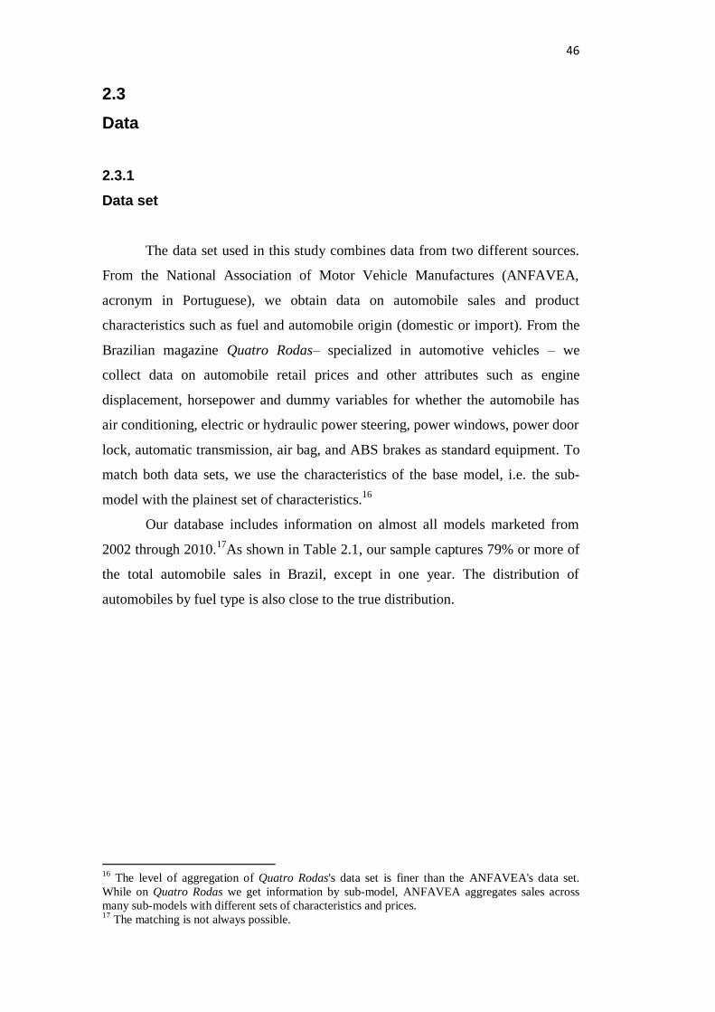
46
2.3
Data
2.3.1
Data set
The data set used in this study combines data from two different sources.
From the National Association of Motor Vehicle Manufactures (ANFAVEA,
acronym in Portuguese), we obtain data on automobile sales and product
characteristics such as fuel and automobile origin (domestic or import). From the
Brazilian magazine Quatro Rodas– specialized in automotive vehicles – we
collect data on automobile retail prices and other attributes such as engine
displacement, horsepower and dummy variables for whether the automobile has
air conditioning, electric or hydraulic power steering, power windows, power door
lock, automatic transmission, air bag, and ABS brakes as standard equipment. To
match both data sets, we use the characteristics of the base model, i.e. the sub-
model with the plainest set of characteristics.16
Our database includes information on almost all models marketed from
2002 through 2010.17
As shown in Table 2.1, our sample captures 79% or more of
the total automobile sales in Brazil, except in one year. The distribution of
automobiles by fuel type is also close to the true distribution.
16
The level of aggregation of Quatro Rodas's data set is finer than the ANFAVEA's data set.
While on Quatro Rodas we get information by sub-model, ANFAVEA aggregates sales across
many sub-models with different sets of characteristics and prices. 17
The matching is not always possible.

47
Table 2.1 Ratio between our sample and ANFAVEA’s data set (%)
Automobile market
Flex-fuel
automobile market
2002 93
2003 86
2004 94 66
2005 72 70
2006 79 78
2007 81 82
2008 83 84
2009 88 90
2010 85 87 Note: To obtain the sample-ANFAVEA ratio, we use the new automobile registrations in Brazil
(reported by ANFAVEA) as proxy for automobiles sales.
Since automobile models enter and exit the sample over the nine-year
study, the number of automobile models in each year changes but, in total, we
have 870 observations. Although we have monthly data set available from both
sources, we set the data set as annual because of the low month-to-month
variation regarding automobile retail prices and characteristics.
For the annual automobile sales, we sum the sales of each month from
January to December. For the automobile characteristics, we use the data set
available for January of each year. Since monthly changes in model characteristics
are not common, we believe this choice does not lead to any biases in general.
One possible exception is the year of 2003 – the year of introduction of the flex-
fuel technology.
The first automobile with the flex-fuel technology was introduced in the
Brazilian automotive market on March 2003, and it appeared in the Quatro Rodas
magazine in the May issue. So, by using the January issue, we may introduce a
potential measurement error which may leads to an attenuation bias in the
estimates of the effect of the flex-fuel technology on automobile sales. By
comparing the share of flex-fuel automobiles in total sales of new automobiles
from ANFAVEA registers with the corresponding number in our annualized
database, the discrepancy between both data sets is relevant for 2003 and,
arguably, for 2004 (Table 2.2).

48
Table 2.2 Share of flex-fuel in total sales of new automobiles (%)
ANFAVEA Our sample
2002 0 0
2003 3 0
2004 22 16
2005 53 52
2006 83 83
2007 91 92
2008 94 95
2009 95 98
2010 95 98
Table 2.3 provides some summary descriptive statistics. From this Table,
some trends can be highlighted. Average sales increased from a low of 1,134 in
2002 to 2,235 in 2010. This increase is associated with a downward trend in
inflation adjusted prices since 2005. To deflate automobile prices we use the
Extended Consumer Price Index provided by the Brazilian Institute of Geography
and Statistics (IBGE, acronym in Portuguese). For imported cars, we also use the
exchange rate provided by the Central Bank of Brazil. All prices are in 2010
Brazilian Real.
Table 2.3 shows that price (in real terms) fall substantially through 2008 to
2010. This average retail price drop may be explained by the Brazilian
government policy of reducing the Tax on Industrialized Products (IPI, in
Portuguese). The IPI reduction was 100% for automobiles with 1.0 liter powered
engine – in the Brazilian market, the less powerful and most common automobiles
–, and 50% for automobiles with cylinder capacity between 1.0 and 2.0 liters. It is
likely that this price reduction boosted automobile demand.
Regarding the flex-fuel technology trend, Table 2.3 shows that the ratio
between flex-fuel and total automobiles18
increased significantly since the flex-
fuel introduction, from 16% to 98%. This upward trend may demonstrate not only
consumers’ preference toward automobiles with this technology, but also
automakers’ decision to produce only flex-fuel automobiles.
Table 2.3 also shows some descriptive statistics relative to other
automobile characteristics. While only 8% of automobiles in Brazil had air
conditioning as standard equipment in 2002, in 2010 the percentage increased to
18
Sale of new automobiles.

49
26%. This trend indicates a more general one toward more extensive standard
equipment. Also, it may suggest that more advanced equipment, such as ABS
brakes, are becoming more accessible for most consumers. However, one must be
careful when interpreting the second part of Table 2.3. It is probably true that for
some characteristics, such as air conditioning, most automobiles are sold with this
equipment. Therefore, we might have measurement errors in our database
regarding, for example, air conditioning, power window and power door locks. As
a result, using these variables could lead to a downward bias.
2.3.2
Understanding the introduction of the flex-fuel technology
Flex-fuel automobiles were introduced by Volkswagen on March 24,
2003. The first automobile with this technology to be sold in Brazil was a new
version of the Gol Total Power 1.6, named Gol Total Flex 1.6. Previously, Gol
Total Power already had two versions: one with gasoline engine and another with
ethanol engine. All the three automobiles had similar standard equipment.
Regarding their performance, the Gol Flex, when fueled with 100% gasoline
(ethanol), had a similar performance – concerning fuel consumption per kilometer
traveled – to Gol Total Power with gasoline (ethanol) engine.19
Because of the
new technology, the retail price of the Gol Total Flex 1.6 was higher than its
counterparts, but the initial price difference – R$ 950,00 – was less than optional
extras such as pearlescent paint. The Gol Total Flex was an immediate success,
with sales equal to 17,936, i.e., 11% of the total sales of Gol Total 1.6, in its first
year.
The rapid acceptance of the Gol Total Flex by Brazilian consumers may be
explained by the ratio between ethanol and gasoline prices. Based on fuel
efficiency, fueling with ethanol is economic advantageous if its price is at least
70% of gasoline price.20
From Figure 2.1, the efficiency ratio is less than 70%
only a few months after Gol Flex was launched which may explain the upward
trend regarding the sales of Gol Total Flex.
19
The tests were done by the Quatro Rodas magazine. 20
The ethanol-gasoline price relation of 70% represents an average and, accordingly to the
National Institute of Metrology, Quality and Technology (INMETRO, acronym in Portuguese) it
may varies from 69% to 72% depending on the engine.

50
Figure 2.1 Ratio between the price of ethanol and the price of gasoline
Source: National Agency of Petroleum, Natural Gas and Biofuels (ANP).
Figure 2.2 shows the initial evolution regarding the quantity sold and the
retail price of the three versions of Gol Total 1.6. Given that the product
characteristics were similar, it appears that consumers prefer to buy flex-fuel
automobiles over gasoline and ethanol powered engine. Regarding the prices, as
the flex-fuel technology becomes cheaper, the difference between prices
decreases.

51
Figure 2.2 Gol Power 1.6 - the first automobile with the flex-fuel technology sold in Brazil
Source: Quatro Rodas magazine.
Other automakers quickly responded, introducing their own versions of
flex-fuel automobiles. In May/June 2003, Chevrolet introduced the flex-fuel
version of the Corsa 1.8 and in July, of the same year, Fiat introduced the Palio
Flex 1.3. So, although Volkswagen was the first automaker to sell flex-fuel
automobiles, it did not own the flex-fuel technology. Consequently, Volkswagen
did not dominate the market of flex-fuel automobiles. The new technology was
well known by all the major players (Volkswagen, Chevrolet, Fiat and Ford) at the
time flex-fuel automobiles were introduced in the Brazilian automotive market. If

52
it was not for uncertainties regarding regulation measures, flex-fuel automobiles
should have been introduced earlier in Brazil.21
Figure 2.3 shows that as soon as the flex-fuel technology was introduced
in the Brazilian automotive market, it has quickly gained market-share.22
This
figure also shows that, over the nine-year study, there was a substitution between
gasoline-powered toward flex-fuel automobiles.
Figure 2.3 Market-shares by fuel type
Notes: To obtain total market-share by fuel for each year, we sum the market-shares of each model
according to fuel type. The market-share of each model is computed as the ratio of its sales (from
our database) to the potential market. Following BLP (1995), we consider that the potential market
equals the number of household. This information is provided by the IBGE.
The substitution pattern, however, was not the same for all automobile
models. In Figure 2.4, we use monthly data from ANFAVEA (from March 2003
through March 2004) to assess what was the percentage of flex-fuel automobiles
in total sales for some models right after the introduction of the new fuel option.
We normalize the data on which the automobiles were introduced to better
visualize the different trajectories. For some models, such as Gol, Corsa
(Chevrolet), and Palio (Fiat), the substitution between gasoline and flex-fuel took
longer than for other automobile models, such as Meriva (Chevrolet) and Fox
(Volkswagen).
21
An important regulatory measure came on August 2002 when the Federal Government decided
that the flex-fuel system should have the same tax rate - IPI - as ethanol engine. 22
To compute the market-share we use the number of households as the potential market. This
data set is provided by the Brazilian Institute of Geography and Statistics (IBGE, acronym in
Portuguese).

53
In Figure 2.5, we use the data set from the Quatro Rodas magazine to
investigate how prices of the new flex-fuel option compared with that of the
gasoline version. We are not able to construct a series of monthly price for each
automobile model as we have done in Figure 2.4 because the prices for many
models are not available consistently (i.e. monthly) in the magazine. So, for each
year, we consider automobile models for which both versions exist (flex-fuel and
gasoline engine) and have the prices available. We can have different automobiles
in each year, but we have the same automobile models for the flex-fuel
automobiles set and for the gasoline engine set. For each year, we take an average
of each set and use it to calculate the ratio between the price of flex-fuel
automobiles and the price of gasoline-powered automobiles. Figure 2.5 presents
evidence that when flex-fuel automobiles were introduced in the Brazilian market,
they were more expensive than their gasoline-powered versions. This situation
reverse as the flex-fuel technology becomes cheaper and as the gasoline versions
become more sophisticated and, thereby, more expensive.23
Indeed, Figure 2.6 shows that gasoline-fueled engine automobiles became,
over the years, more associated with more sophisticated automobiles– most of
them imported – which may help explain the rise in prices in real terms.24
This
general trend is confirmed when we compare the other product characteristics.
While flex-fuel automobiles followed a similar trend to the Brazilian automotive
market, the observed trend regarding gasoline engine automobiles attributes
indicates an expansion of almost all characteristics considered in this study as
standard equipment (Table 2.4).
23
Ideally we would like to compare exactly the same automobile models except for the flex-fuel
technology. From our database, however, this kind of comparison is not possible. The automobile
models differ regarding other characteristics besides the flex-fuel. 24 The circles represent the size of each market, flex-fuel and gasoline automobiles.
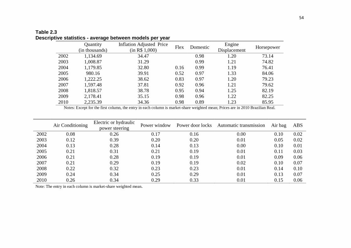
54
Table 2.3 Descriptive statistics - average between models per year
Quantity
(in thousands)
Inflation Adjusted Price
(in R$ 1,000) Flex Domestic
Engine
Displacement Horsepower
2002 1,134.69 34.47 0.98 1.20 73.14
2003 1,008.87 31.29 0.99 1.21 74.82
2004 1,179.85 32.80 0.16 0.99 1.19 76.41
2005 980.16 39.91 0.52 0.97 1.33 84.06
2006 1,222.25 38.62 0.83 0.97 1.20 79.23
2007 1,597.48 37.81 0.92 0.96 1.21 79.62
2008 1,818.57 38.78 0.95 0.94 1.25 82.19
2009 2,178.41 35.15 0.98 0.96 1.22 82.25
2010 2,235.39 34.36 0.98 0.89 1.23 85.95 Notes: Except for the first column, the entry in each column is market-share weighted mean; Prices are in 2010 Brazilian Real.
Air Conditioning Electric or hydraulic
power steering Power window Power door locks Automatic transmission Air bag ABS
2002 0.08 0.26 0.17 0.16 0.00 0.10 0.02
2003 0.12 0.39 0.20 0.20 0.01 0.05 0.02
2004 0.13 0.28 0.14 0.13 0.00 0.10 0.01
2005 0.21 0.31 0.21 0.19 0.01 0.11 0.03
2006 0.21 0.28 0.19 0.19 0.01 0.09 0.06 2007 0.21 0.29 0.19 0.19 0.02 0.10 0.07
2008 0.22 0.32 0.23 0.23 0.01 0.14 0.10
2009 0.24 0.34 0.25 0.29 0.01 0.13 0.07
2010 0.26 0.34 0.29 0.33 0.01 0.15 0.06
Note: The entry in each column is market-share weighted mean.

55
Figure 2.4 Share of flex-fuel automobiles relative to total automobile sales - by model
Months since introduction
Note: we use the data set from ANFAVEA. We use monthly data from March 2003 through
March 2004.
Figure 2.5 Ratio between the price of flex-fuel automobiles and the price of gasoline engine automobiles
Note: we use annual data. Using the data set from the Quatro Rodas magazine we are not able to
construct a series of monthly price for each automobile model as we have done in Panel A. So, for
each year, we consider automobile models that have both versions, flex-fuel and gasoline engine,
and for which we have the price of both version. We can have different automobiles in each year,
but we have the same automobile models for the flex-fuel automobiles set and for the gasoline
engine set. For each year, we take an average of each set and use it to calculate the ratio between
the price of flex-fuel automobiles and the price of gasoline-powered automobiles.

56
Figure 2.6 Descriptive statistics by fuel type

57
Table 2.4 Descriptive statistics by fuel type (cont.)
Air
Conditioning
Electric or
hydraulic
power
steering
Power
window
Power
door
locks
Automatic
transmission
Air
bag ABS
Panel A: : Gasoline-Powered Automobiles
2002 0.09 0.26 0.17 0.16 0.00 0.10 0.02
2003 0.13 0.39 0.20 0.20 0.01 0.05 0.02
2004 0.16 0.29 0.18 0.17 0.00 0.12 0.02
2005 0.33 0.40 0.35 0.32 0.01 0.21 0.06
2006 0.77 0.79 0.72 0.72 0.05 0.49 0.16
2007 0.78 0.79 0.75 0.75 0.20 0.64 0.43
2008 0.99 0.99 0.99 0.99 0.24 0.90 0.89
2009 1.00 1.00 1.00 1.00 0.59 0.99 1.00
2010 1.00 1.00 1.00 1.00 0.69 1.00 0.98
Panel A: : Flex-fuel Automobiles
2002 - - - - - - -
2003 - - - - - - -
2004 0.00 0.29 0.00 0.00 0.00 0.00 0.00
2005 0.10 0.22 0.10 0.08 0.00 0.03 0.00
2006 0.09 0.18 0.08 0.08 0.00 0.00 0.04
2007 0.16 0.25 0.14 0.14 0.01 0.05 0.04
2008 0.18 0.29 0.19 0.19 0.00 0.10 0.05
2009 0.22 0.32 0.23 0.28 0.00 0.11 0.05
2010 0.24 0.33 0.28 0.32 0.00 0.13 0.04
From the supply side, Figure 2.7 shows that the production of flex-fuel
automobiles followed an upward trend since its introduction in 2003. Similarly to
the trajectory of the demand for automobiles, the production of gasoline-fueled
engine automobiles fell sharply over the nine-year study. The decision to produce
flex-fuel instead of gasoline cars was endorsed by most automobile producers in
Brazil and, in 2007, accordingly to our database, buying an economy car with
gasoline engine was already a hard task.
Besides several gasoline fueled automobiles being converted to flex-fuel
cars, most new automobile launches refers to flex-fuel automobiles. Thus,
although, at the beginning, flex-fuel automobiles were offer as an alternative to
gasoline or ethanol engine automobiles, few years later its introduction, flex-fuel
represents the only available option for some categories.

58
Figure 2.7 Automobile production in Brazil (in units)
About the conversion, it appears, from our data analysis, that the gasoline-
fueled automobile converted into flex-fuel has the same standard equipment as its
gasoline version although the flex-fuel automobile has more horsepower.25
Regarding the engine displacement, the trend is not that obvious. While for some
automobiles the engine displacement increases, for example, from 1.0 to 1.4, for
other it has remained unaltered. Nevertheless, it is difficult to relate this changes
to the flex-fuel technology since the automotive industry is always innovating
towards automobiles with better performance and better benefits for consumers.
To gain some basic intuitions about the relationship between the flex-fuel
technology and other automobile characteristics, we run hedonic regressions of
price on observable characteristics.26
Table 2.5 presents evidence of a spurious correlation between flex-fuel and
the other attributes, indicating that we should control for other characteristics to
eliminate the bias from this correlation. Column 1 shows that flex-fuel
automobiles are cheaper than the gasoline-powered automobiles. When we control
for market fixed effects and for other characteristics the difference between both
automobiles decreases significantly, from 84% to 4.96%. Column 6 shows that
when we introduce automobile models fixed effects, the flex-fuel technology
becomes marginally important to consumers. Although we should not draw major
25
The comparison is done when flex-fuel cars are fueled with 100% gasoline. 26
The hedonic approach states that the coefficients of the regression should be interpreted as
marginal implicit price, i.e., the intrinsic value of each attribute.

59
conclusions from Table 2.5, the results found corroborate with the stylized fact
presented previously in our database analysis: automobile prices tend to be equal,
or very similar, when comparing, within the same year, automobile models that
only differ in having the flex-fuel technology or not.
Table 2.5 Hedonic price model results
(1) (2) (3) (4) (5) (6)
Variables ln(price) ln(price) ln(price) ln(price) ln(price) ln(price)
Flex-fuel -0.840*** -1.207*** -0.00798 -0.0496*** 0.120*** 0.0250*
(0.0432) (0.0542) (0.0191) (0.0156) (0.0255) (0.0128)
Ethanol
-0.0707* -0.0536 -0.0303
(0.0408) (0.0380) (0.0207)
Origin (1 = domestic)
-0.103*** -0.121*** -0.109***
(0.0249) (0.0220) (0.0339)
ln(engine displacement)
0.130 -0.0211 -0.00201
(0.0855) (0.0793) (0.0539)
ln(horsepower)
1.109*** 1.305*** 0.531***
(0.0772) (0.0736) (0.0675)
Air conditioning
0.0185 0.0277 0.0626***
(0.0196) (0.0219) (0.0162)
Electric or hydraulic power steering
0.00724 -0.00295 0.0425*
(0.0244) (0.0257) (0.0223)
Power window
0.0289 -0.00149 -0.0406
(0.0413) (0.0468) (0.0281)
Power door locks
0.000682 0.0604 0.0716***
(0.0386) (0.0445) (0.0244)
Automatic transmission
0.382*** 0.373*** 0.106***
(0.0387) (0.0329) (0.0364)
Airbag
0.0476** 0.0449** 0.0374*
(0.0229) (0.0228) (0.0203)
ABS brakes
0.0801*** 0.0881*** 0.0746***
(0.0263) (0.0244) (0.0256)
Constant 11.51*** 11.15***
5.674*** 4.911***
(0.0383) (0.0804)
(0.321) (0.309)
Market fixed effects? N Y Y N Y Y Automobile models
fixed effects? N N Y N N Y
Observations 870 870 870 870 870 870
R-squared 0.158 0.282 1.000 0.919 0.935 1.000
All in all, the data analysis suggests that the introduction of the flex-fuel
technology was rapid and it was not exogenous to other characteristics. The flex-
fuel technology was first introduced in economy and compact automobiles – the
plainest and most common automobiles in Brazil. This finding suggests, therefore,
a correlation between flex-fuel and other attributes that must be taken into account
when estimating the full model.

60
2.4
Model
In this section, we present the methodology to estimate the demand
parameters. Theoretically, we follow the discrete choice literature for
differentiated products and obtain the aggregate demand by aggregating individual
decisions. Different from the traditional discrete choice literature, demand is
characterized by a set of continuous variables – representing the market-shares –
instead of discrete variables. Empirically, we use the techniques developed in
Berry (1994) and BLP (1995) to estimate demand and supply curves based solely
on product-level data.
2.4.1
Theory: demand
The demand for an automobile model, 𝑗, in a given year, is obtained by
aggregating the individual probabilities of buying 𝑗.
Within the automotive context, each consumer faces a choice among 𝐽 + 1
alternatives: 𝐽 automobile models and an outside alternative that represents the
option of not buying any automobile.27
For each one of these alternatives,
consumer 𝑖 derives a certain level of utility, 𝑢𝑖𝑗.
Following Berry (1994), we assume that the utility of consumer 𝑖 for an
automobile model 𝑗 is a function of both product characteristics, 𝑥𝑗, and
consumers characteristics, 𝜈𝑖: 𝑢𝑖𝑗 = 𝑈(𝑥𝑗 , 𝜉𝑗 , 𝑝𝑗 , 𝜈𝑖; 𝜃), where 𝜉𝑗 and 𝑝𝑗 are the
unobserved (by the econometrician) characteristics and the price of an automobile
model 𝑗 respectively; 𝜃 represents the demand parameters. The term 𝜈𝑖 captures
taste preferences of consumer 𝑖 regarding product characteristics. As we do not
have consumer-level data, we assume 𝜈 has a known distribution. In this study,
we follow BLP (1995) and assume that 𝜈𝑖 has a standard normal distribution.
Given the primitives of the model, consumer 𝑖 chooses 𝑗 if and only if:
27
The existence of the outside alternative is a key factor to estimate the aggregate demand; it
allows, for example, that the market demand declines if all within-market price increase.

61
𝑈(𝑥𝑗 , 𝜉𝑗 , 𝑝𝑗 , 𝜈𝑖; 𝜃) ≥ 𝑈(𝑥𝑞, 𝜉𝑞, 𝑝𝑞 , 𝜈𝑖; 𝜃), 𝑞 = 0,1,… , 𝐽
Where alternative zero, or outside good, represents the option of not
buying an automobile.
Assuming ties occur with zero probability, the individual probability of
choosing 𝑗 is:
𝑃𝑖𝑗 = Pr(𝑈(𝑥𝑗 , 𝜉𝑗 , 𝑝𝑗 , 𝜈𝑖; 𝜃) > 𝑈(𝑥𝑞, 𝜉𝑞, 𝑝𝑞 , 𝜈𝑖; 𝜃) ∀𝑗 ≠ 𝑞)
As in the traditional discrete choice literature, 𝑃𝑖𝑗 equals the individual
demand for product 𝑗. The aggregate demand for product 𝑗 is given by ∫𝑃𝑖𝑗𝑑𝜈,
where 𝑑𝜈 provides the density of 𝜈 in the population. Different from the
traditional approach, 𝑃𝑖𝑗 is not discrete and ∫𝑃𝑖𝑗𝑑𝜈 is interpreted as the fraction of
consumers that buy automobile model 𝑗, i.e., the market-share,
𝑠𝑗(𝑥𝑗 , 𝑝𝑗 , 𝜉𝑗, 𝑑𝜈; 𝜃).28
For tractability reasons, the utility function is separable in two terms: one
determined by the product characteristics (𝛿𝑗) and one determined by consumer
characteristics (𝜇𝑖𝑗), 𝑢𝑖𝑗 = 𝛿𝑗 + 𝜇𝑖𝑗 , where 𝛿𝑗 = 𝑥𝑗𝛽 − 𝛼𝑝𝑗 + 𝜉𝑗and 𝜇𝑖𝑗 = 𝜖𝑖𝑗. As
it is common in traditional logit models, we assume that 𝜖𝑖𝑗 is independent and
identically distributed (IID) across consumers. As a result, assuming that the
variation in consumer tastes enters only through the additive term 𝜖𝑖𝑗 imposes
strong restrictions on the estimated own- and cross-price elasticities.
In traditional logit models, price elasticities are determined only by the
market-shares, i.e., conditional on market-shares, substitution patterns do not
depend on the observable product characteristics (BLP (1995)). This limitation of
the logit models is well known in the discrete choice model literature and it is
formally called Independence of Irrelevant Alternatives.
To overcome this problem, we assume that the utility function is described
by the traditional random coefficient model and we allow for interaction between
individual and product characteristics. In this case, consumers with different
28
To be more specific, the demand for automobile model 𝑗 is 𝑀𝑠𝑗, where 𝑀 is the number of
consumers in the automotive market and sj is the market-share of good j.

62
preferences will have different utility levels and induce different substitution
patterns. Within this model context, the own- and cross-price elasticities depend
not only on market-share, but also on consumers and product characteristics. The
substitution patterns obtain through this model are more realistic and more in
accordance with economic theory.
Within this context, the utility obtained from buying an automobile model
𝑗 in a given year, 𝑡, 29 is:
𝑢𝑖𝑗𝑡 = 𝑥𝑗𝑡𝛽 + 𝜉𝑗𝑡 + 𝛼∗ ln(𝑦𝑖 − 𝑝𝑗) + ∑ 𝜎𝑘𝑥𝑗𝑡𝑘𝜐𝑖𝑘𝑘 + 𝜖𝑖𝑗𝑡 Eq.1
Where:
𝛿𝑗𝑡 = 𝑥𝑡𝑗𝛽 + 𝜉𝑗𝑡 Eq. 1.a
𝜇𝑖𝑗𝑡 = 𝛼∗ ln(𝑦𝑖 − 𝑝𝑗) + ∑ 𝜎𝑘𝑥𝑗𝑡𝑘𝜈𝑖𝑘 + 𝜖𝑖𝑗𝑡𝑘 Eq. 1.b
Where 𝛿𝑗 is interpreted as the mean utility, 𝜇𝑖𝑗 is the deviation regards this
mean and 𝜃 = (𝛼∗, 𝛽, 𝜎) is the demand parameters vector we are interested in.
Note that Equation 1 is slightly different from the logit specification. In the latter,
price is introduced in the mean utility term while in Equation 1, following the
BLP specification, we interact price with income.30
Now, consumers with
different income levels respond different to price changes.31
Besides, to better
capture the income effects, we allow the price coefficient to vary with different
income groups.
𝛼∗ = {
𝛼1,𝛼2,𝛼3,
𝑦𝑖 ≤ �̅�1
�̅�1 < 𝑦𝑖 ≤ �̅�2
𝑦𝑖 > �̅�3
About the coefficients interpretation in Equation 1, the contribution of the
𝑘𝑡ℎ product characteristic, 𝑥𝑘, to the utility of consumer 𝑖 is (𝛽𝑘 + 𝜎𝑘𝜈𝑖𝑘) which
depends on consumer preferences. Regarding the individual tastes, we assume that
preferences do not change over years. This hypothesis is reasonable within a
durable good market context.
29
In BLP (1995), different years are interpreted as different markets. 30
Besides the characteristics of the good purchased, utility is now also a function of expenditures
on other goods and services. 31
Adding demographics characteristics, such as income, improves the precision of the estimator.
63
To complete the model description, the utility level of not buying an
automobile is:
𝑢𝑖0𝑡 = 𝛼∗𝑙𝑛(𝑦𝑖) + 𝜉0𝑡 + 𝜎0𝜐𝑖0 + 𝜖𝑖0𝑡
As we do not have information about the outside alternative and the
market-shares depend on differences in utility,32
we normalize the mean utility of
the outside alternative to zero (𝛿0 = 𝜉0 = 0) and add a constant term in the utility
function of the inside goods.
Finally, for tractability reasons, we assume that 𝜖𝑖𝑗 is IID type 1 extreme
value, with density 𝑓(𝜖𝑖𝑗) = 𝑒−𝜀𝑖𝑗 exp(−𝑒𝜖𝑖𝑗). This assumption guarantees a
closed form for the individual probabilities.
𝑃𝑖𝑗 =𝑒
𝛿𝑗+𝜇𝑖𝑗
1+∑ 𝑒𝛿𝑞+𝜇𝑖𝑞
𝑞
Eq.2
Knowing the probabilities functional forms, however, do not solve the
problem of computing the integral, ∫𝑃𝑖𝑗𝑃(𝑑𝜈). To solve this computational
problem, we follow BLP (1995) and aggregate via simulation, i.e., we take ns
random draws from the distribution on 𝜈 and compute:
𝑠𝑗(𝑥𝑗 , 𝑝𝑗 , 𝜉𝑗, 𝑑𝜈; 𝜃) =1
𝑛𝑠∑
𝑒𝛿𝑗+𝜇𝑖𝑗
1+∑ 𝑒𝛿𝑞+𝜇𝑖𝑞
𝑞
𝑛𝑠𝑖=1 Eq.3
32
Considering the logit model, for example, we have that the individual probability of buying the
automobile model 𝑗 is 𝑃𝑖𝑗(𝑢𝑖𝑗 > 𝑢𝑖𝑞, 𝑎𝑙𝑙 𝑗 ≠ 𝑞) = 𝑃𝑖𝑗(𝑢𝑖𝑞 − 𝑢𝑖𝑗 < 0, 𝑎𝑙𝑙 𝑗 ≠ 𝑞) = 𝑃𝑖𝑗(𝜖𝑖𝑗 −
𝜖𝑖𝑞 < 𝛿𝑗 − 𝛿𝑞, 𝑎𝑙𝑙 𝑗 ≠ 𝑞).

64
2.4.2
Estimation procedure
To estimate the demand parameters in Equation 1 we follow the
methodology developed in BLP (1995).
(i) Step 1 – Estimate the market-shares predicted by the model
The predicted market-shares, as well as the means of the consumers’
utility, are obtained via iteration.
From the theory section, we know that the demand for an automobile
model is given by the market-share of this model in the automotive market.
Therefore, to obtain our demand system, we match the observed market-shares,
𝑆𝑗, to the market-shares that are computed using Equation 3, 𝑠𝑗(𝑥𝑗 , 𝑝𝑗 , 𝜉𝑗 , 𝑑𝜈; 𝜃).
𝑆𝑗 = 𝑠𝑗(𝑥𝑗 , 𝑝𝑗 , 𝜉𝑗, 𝑑𝜈; 𝜃) = 𝑠𝑗(𝛿𝑗 , 𝑑𝜈; 𝜃) Eq.4
Equation 4 implicitly determines the mean utility levels, 𝛿. Solving
Equation 4, however, is not straightforward. The nonlinearity of Equation 4
prevents estimating the demand parameters analytically. Besides, as pointed out in
Berry (1994), the presence of the unobserved product characteristics raises a
difficult econometric problem: endogeneity in a nonlinear context. It is likely that
price is positively correlated to the unobserved product characteristics.33
As a
result, if price endogeneity is not control for, then we would expect price
coefficient to be attenuated. Our results would show that consumers respond less
to changes in price than in reality.
To control for the price endogeneity in Equation 4, we use the
Instrumental Variables (IV) approach. However, because of the nonlinearity of the
33
To account for the potential correlation between the unobserved and all the other observed
characteristics, we would have to model the choice of all the observed product characteristics. In
this study, given that the relationship between the price and the unobserved characteristics is more
direct, we take into account only the price endogeneity. Besides, following BLP (1995), we
assume that price is the only choice-variable in the firm problem. For more details, see Ackerberg
et al. (2007).

65
demand system, we must first transform Equation 4 so that the unobserved
product characteristics enter demand systems in a linear fashion.
Berry (1994) proposes transforming Equation 4 by inverting the predicted
market-shares, i.e., 𝛿𝑗 = 𝑠𝑗−1(𝑆𝑗). This inversion transforms the demand system in
a system of equations that is linear in the unobservable product characteristics,
allowing us to use the traditional IV approach.34
Berry (1994) also shows that after some algebra and given the type 1
extreme value distribution of 𝜖𝑖𝑗, the mean utility is determined by:
𝛿𝑗 = ln(𝑆𝑗) − ln (𝑠𝑗(𝑥𝑗 , 𝑝𝑗 , 𝜉𝑗 , 𝑑𝜈; 𝜃))
BLP (1995) show that solving Equation 4 is equivalent to solve:
𝛿𝑗 = 𝛿𝑗 + ln(𝑆𝑗) − ln (𝑠𝑗(𝑥𝑗 , 𝑝𝑗 , 𝜉𝑗 , 𝑑𝜈; 𝜃)) Eq. 5
Therefore, from Equation 5, we find 𝛿 recursively. For some initial guess
for 𝛿, 35 we obtain a new 𝛿, say 𝛿′, as the output of Equation 5. We then substitute
𝛿′ in the right-hand side and compute the market-shares and obtain a new value
for the mean utility. This procedure is repeated until convergence is achieved.
Regarding the tolerance level for this initial step, we use 10-14
. Dubé, Fox
and Su (2012) argue that loose tolerance for the contraction mapping leads to
incorrect parameters estimates and even the failure of the optimization routine to
converge. Thus, using 10-14
for the inner loop is a conservative choice to eliminate
the inner-loop numerical error.36
Before going to the second step, one may notice that the nonlinear search
is only over the demand parameters associated with the heterogeneity between
consumers, i.e., 𝜎. Therefore, we are able to separate the parameters of the
demand into two vectors, 𝜃1 = 𝛽 and 𝜃2 = (𝛼∗, 𝜎), where 𝜃1 and 𝜃2 correspond
to the linear and nonlinear parameters respectively.
34
See Berry (1994) for more details about the transformation. 35
Our first guess for the mean utility is the 𝛿 obtained via IV Logit. So, before estimating the
random coefficients model, we estimate the demand parameters assuming no heterogeneity
between consumers. 36
For the outer loop, we use 10-6
.

66
All in all, in this first step we estimate the mean utility as a function of the
nonlinear demand parameters, 𝛿(𝜃2). In the next step, using the mean utility
implied by the observed and predicted market-shares, we solve for the demand
unobservables.
(ii) Step 2 – Solve for the demand unobserved product characteristics
Once we have the mean utility vector, 𝛿(𝜃2), we are able to solve for the
demand unobservables using Equation 1.a.
𝜉𝑗 = 𝛿𝑗(𝜃2) − 𝑥𝑗𝛽 Eq. 6
Notice that the linear parameters 𝜃1 are a function of the nonlinear
parameters and are estimated by Two Stage Least Square.
𝜃1 = (𝑋′𝑍𝐴−1𝑍′𝑋)−1𝑋′𝑍𝐴−1𝑍′𝛿(𝜃2)
Where 𝑋 is the matrix of the characteristics of the automobiles (excluding
the price), 𝑍 is the matrix of instruments and 𝐴 = (𝑍′𝑍) is the weighting matrix.
(iii) Step 3 – Calculate the optimal instruments and define the moment
conditions
Following BLP (1995), we use product characteristics – excluding the
product characteristics of the model been studied – in a given year as instrument
for the price in Equation 6. More specifically, BLP (1995) proposes using as
instrument a function of the characteristics of other automobile models produced
by the same firm and by the competing firms.
The reason for choosing these instruments comes from the oligopoly
theory. It is well known that in oligopoly markets, firms set their prices above
their marginal cost. So, the decision of the firm depends on the characteristics of
products produced by the given firm and likely by the rival firm. The relationship
between these characteristics affects demand only via price.
67
The set of instruments for the price proposed in BLP (1995) is the sum of
the characteristics of the products produced by the same firm – ∑ 𝑥𝑞𝑘𝑞≠𝑗,𝑞∈𝐹𝑓 –
and the sum of the characteristics produced by the competing firms –
∑ 𝑥𝑞𝑘𝑞≠𝑗,𝑞∉𝐹𝑓, where 𝐹𝑓 is the set of products produced by firm 𝑓 and 𝑘 is the 𝑘th
product characteristic produced by firm 𝑞. In this study, however, instead of using
the sum, we opt for using the mean. First stages regressions analysis indicates
that, for this study, the mean is a stronger instrument than the sum.37
Once we have the optimal instruments, we are able to determine our
sample moment conditions:
𝐺𝑗 =1
𝐽∑𝐻𝑗(𝑧)𝜉𝑗
𝐽
𝑗=1
Where 𝐻(𝑧) represents the matrix of instruments which includes the
instruments for the price and the exogenous characteristics in Equation 6.
The optimization procedure consists in estimating the demand parameters,
𝜃, that minimizes:
‖𝐺𝑗‖ = ‖1
𝐽∑ 𝐻𝑗(𝑧)𝜉𝑗
𝐽𝑗=1 ‖, where ‖𝐺𝑗‖ = 𝐺′𝑗𝐺𝑗
(iv) Step 4 – Compute the demand parameters standard-deviations
The final step consists in estimating the variance-covariance matrix of the
estimated demand parameters. We use the asymptotic variance of the nonlinear
Generalized Method of Moments estimator.
�̂�(�̂�) = 𝑁[�̂�′𝑍𝐴−1𝑍′�̂�]−1
[�̂�′𝑍𝐴−1�̂�𝐴−1𝑍′�̂�][�̂�′𝑍𝐴−1𝑍′�̂�]−1
Where �̂� =𝜕𝜉
𝜕𝜃′ and �̂� =
1
𝑁∑ 𝜉𝑗𝑍𝑗𝑍′𝑗𝑗 .
37
We test the instruments by estimating the IV logit model.
68
To estimate the parameters of the supply side, we also follow the framework
presented in BLP (1995)
(i) Step 1 – calculate the markups
Following the BLP methodology, markups are computed as a function of
the parameters of the demand system and price.
𝑏(𝑝, 𝑥, 𝜉; 𝜃) = Δ(𝑝, 𝑥, 𝜉; 𝜃)−1𝑠𝑗 (𝑥𝑗, 𝑝𝑗, 𝜉
𝑗, 𝑑𝜈;𝜃)
Where 𝑏(𝑝, 𝑥, 𝜉; 𝜃) is the markup and Δ(𝑝, 𝑥, 𝜉; 𝜃) is a 𝐽 × 𝐽 matrix whose
(𝑗, 𝑟) element is given by:
∆𝑗𝑟= {
−𝜕𝑠𝑟
𝜕𝑝𝑗, if 𝑗 and 𝑟 are produced by the same firm
0, otherwise
Where:
−𝜕𝑠𝑗
𝜕𝑝𝑗= ∫𝑃𝑖𝑗(1 − 𝑃𝑖𝑗)
𝜕𝜇𝑖𝑗
𝜕𝑝𝑗𝑃(𝑑𝜈) and
−𝜕𝑠𝑗
𝜕𝑝𝑟= ∫−𝑃𝑖𝑗𝑃𝑖𝑟
𝜕𝜇𝑖𝑞
𝜕𝑝𝑞𝑃(𝑑𝜈)
(ii) Step 2 – Obtain the pricing equation
We estimate the parameters of the supply side via Ordinary Least Square
(OLS). The supply curve is given by the following pricing equation:
𝑙𝑛(𝑝 − 𝑏(𝑝, 𝑥, 𝜉; 𝜃)) = 𝑤𝛾 + 𝜔
2.5
Results
Other than retail prices, we use nine observable automobile characteristics:
engine displacement, horsepower, and dummy variables indicating whether the
automobile is domestically produced, has the flex-fuel technology, air
conditioning, electric or hydraulic power steering, automatic transmission, airbag,

69
and ABS brakes. For all of these variables, we assigned random coefficients –
taste parameters – based on normal draws. 38
Tables 2.6 and 2.7 show the results for our specifications. In total, three
demand models are estimated: OLS Logit, Two Stage Least Square (TSLS) Logit
with IV correction, and random coefficients with IV correction. For the first two
models, we assume that consumers have homogenous preferences. Although this
assumption leads to unrealistic substitution patterns, estimating these models is
useful for baseline comparisons with the full model, i.e., with the random
coefficient model.
Table 2.6 shows that not controlling for price endogeneity leads, as
expected, to attenuated estimates. Column 2 shows that when we control for the
simultaneity bias, the coefficient on price more than doubles. Its magnitude,
however, is still low. Regarding the flex-fuel coefficient, it is robust to the new
estimation strategy and statistically significant, suggesting that the average
consumer likes flex-fuel automobiles. The magnitude of the flex-fuel coefficient,
however, is high relatively to the price coefficient. In Column 2, for example, the
flex-fuel parameter is more than 100 times the price parameter, suggesting that
consumers would be willing to pay a premium of more than R$ 100,000 for an
automobile with flex-fuel technology. This finding is unrealistic.
Table 2.6 also shows that, besides changing the price coefficient, the use
of instruments39
generates changes in some of the parameter estimates. Most
characteristics now enter the utility positively, but for a few attributes, such as
power steering and airbag, the negative signal remains. Also, because of the
strong relationship between the variables, most characteristics are not statistically
significant. Eliminating one of these variables, however, would potentially
aggravate the omitted variable bias.
Based on the descriptive analysis, we also introduce a dummy variable for
the year of 2005 in both models. Different from other years, in 2005 we were not
able to obtain a good match between the data sets from Anfavea and Quatro
Rodas. As a result, we have somewhat discrepant values for this year on, for
38
Normal distribution with mean vector zero and an identity covariance matrix. 39
In total, we have 16 instruments. As in BLP (1995), we choose arbitrarily which potential
instruments to leave in and out because of the near multicollinearity between them.
70
example, sales and retail prices. So, to control for potential bias in our sample,40
we introduce the 2005 dummy variable.
All in all, Table 2.6 shows that taking into account price endogeneity
matters. The importance of the unobservable characteristics can also be seen from
the simple logit specification: 38% of the variance in the mean utility level is due
to unobserved characteristics. Logit models, however, are known for having
unrealistic substitution patterns. The homogenous hypothesis regarding
consumers’ preference implies that price elasticity is a function solely of market-
shares. So, to overcome this and estimate more reliable estimates, we estimate the
random coefficient model (or full model).
40
From the descriptive analysis, it seems that our sample in 2005 has more sophisticated
automobiles, with higher prices, engine displacement and horsepower.
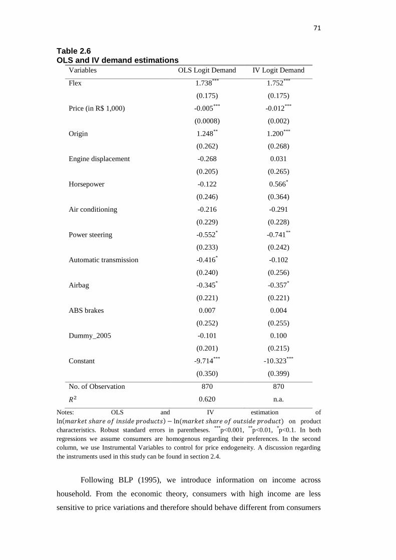
71
Table 2.6 OLS and IV demand estimations
Variables OLS Logit Demand IV Logit Demand
Flex 1.738***
1.752***
(0.175) (0.175)
Price (in R$ 1,000) -0.005***
-0.012***
(0.0008) (0.002)
Origin 1.248**
1.200***
(0.262) (0.268)
Engine displacement -0.268 0.031
(0.205) (0.265)
Horsepower -0.122 0.566*
(0.246) (0.364)
Air conditioning -0.216
-0.291
(0.229) (0.228)
Power steering -0.552*
-0.741**
(0.233) (0.242)
Automatic transmission -0.416*
-0.102
(0.240) (0.256)
Airbag -0.345*
-0.357*
(0.221) (0.221)
ABS brakes 0.007 0.004
(0.252) (0.255)
Dummy_2005 -0.101 0.100
(0.201) (0.215)
Constant -9.714***
-10.323***
(0.350) (0.399)
No. of Observation 870 870
𝑅2 0.620 n.a.
Notes: OLS and IV estimation of
ln(𝑚𝑎𝑟𝑘𝑒𝑡 𝑠ℎ𝑎𝑟𝑒 𝑜𝑓 𝑖𝑛𝑠𝑖𝑑𝑒 𝑝𝑟𝑜𝑑𝑢𝑐𝑡𝑠) − ln (𝑚𝑎𝑟𝑘𝑒𝑡 𝑠ℎ𝑎𝑟𝑒 𝑜𝑓 𝑜𝑢𝑡𝑠𝑖𝑑𝑒 𝑝𝑟𝑜𝑑𝑢𝑐𝑡) on product
characteristics. Robust standard errors in parentheses. ***
p<0.001, **
p<0.01, *p<0.1. In both
regressions we assume consumers are homogenous regarding their preferences. In the second
column, we use Instrumental Variables to control for price endogeneity. A discussion regarding
the instruments used in this study can be found in section 2.4.
Following BLP (1995), we introduce information on income across
household. From the economic theory, consumers with high income are less
sensitive to price variations and therefore should behave different from consumers

72
with low income when deciding to buy (or not) an automobile. To help to capture
the income effects, besides assuming a convex form for the interaction between
price and income, we have also considered three income groups. Based on the
National Household Sample Survey (PNAD, acronym in Portuguese), we
determine the three income group thresholds: the low- and middle-income group,
with annual income up to R$ 30,000; the high-income group, with annual income
between R$ 30,000 and R$ 140,000; and, finally, the top 1% with annual income
higher than R$ 140,000.41
Table 2.7 shows the demand parameters obtained using the full model.42
Now, the effect of each product characteristics on utility varies across consumers
so that we estimate a mean and a standard deviation for each attribute.
Specifically about the flex-fuel technology, the positive sign of the mean taste
coefficient for flex-fuel technology corroborates the results obtained when
assuming no heterogeneous preferences and suggests that the average consumer
likes flex-fuel automobiles. However, the mean taste parameter is not statistically
significant at 10% significance level, indicating that, although the point estimate is
in accordance with the previous estimate, we cannot rule out the possibility that
the average consumer does not care about flex-fuel technology. Interestingly, the
standard deviation for the flex-fuel technology is statistically significant,
suggesting divergence between consumers’ preference.
About the disposable income coefficients, we find, as expected, that
consumers with high income are less sensitive to price variation: we find that
while an increase of R$ 1,000 (about 3%) in the average price of automobiles
decreases the utility of consumers in the middle income group by 0.48%, the
decrease is about 0.05% for consumers in the top 1% income group.43
These
values are smaller than expected initially. When we compare the disposable
income coefficients with the coefficients obtained in Petrin (2002) and Furlong
(2010), both for the United States, the difference is substantial. For the low
income group, for example, Petrin (2002) finds a price coefficient equal to 4.92
and Furlong (2014), 1.013. For the high income group, the difference is even
41
All prices are in January 2010 Brazilian Reais. 42 In Appendix A, we show the result for a simpler model. We assume that, besides income,
consumers differ regarding their preferences toward flex-fuel and the outside good (constant term). 43
To calculate the effect of a price change on consumers’ utility, we use the average income of
each income group and the weight average price of automobile. All measures are for the year of
2010.
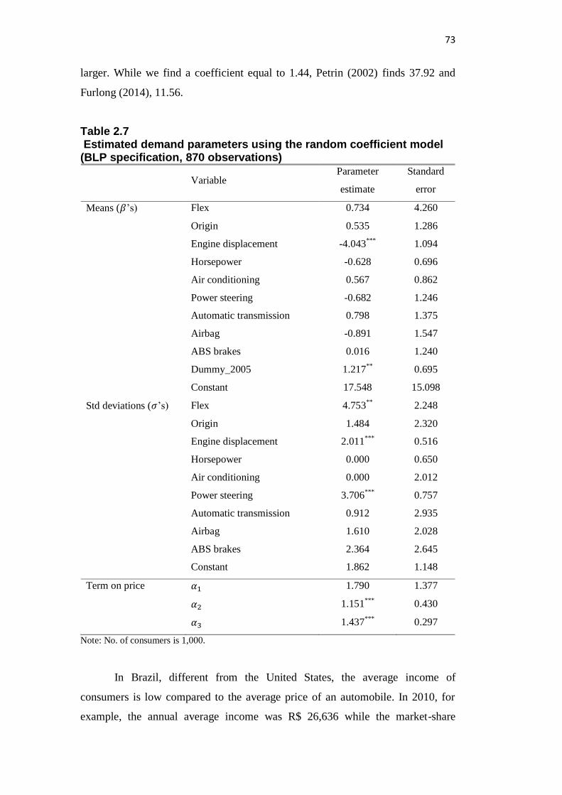
73
larger. While we find a coefficient equal to 1.44, Petrin (2002) finds 37.92 and
Furlong (2014), 11.56.
Table 2.7 Estimated demand parameters using the random coefficient model (BLP specification, 870 observations)
Variable
Parameter
estimate
Standard
error
Means (𝛽’s) Flex 0.734 4.260
Origin 0.535 1.286
Engine displacement -4.043***
1.094
Horsepower -0.628 0.696
Air conditioning 0.567 0.862
Power steering -0.682 1.246
Automatic transmission 0.798 1.375
Airbag -0.891 1.547
ABS brakes 0.016 1.240
Dummy_2005 1.217**
0.695
Constant 17.548 15.098
Std deviations (𝜎’s) Flex 4.753**
2.248
Origin 1.484 2.320
Engine displacement 2.011***
0.516
Horsepower 0.000 0.650
Air conditioning 0.000 2.012
Power steering 3.706***
0.757
Automatic transmission 0.912 2.935
Airbag 1.610 2.028
ABS brakes 2.364 2.645
Constant 1.862 1.148
Term on price 𝛼1 1.790 1.377
𝛼2 1.151***
0.430
𝛼3 1.437***
0.297
Note: No. of consumers is 1,000.
In Brazil, different from the United States, the average income of
consumers is low compared to the average price of an automobile. In 2010, for
example, the annual average income was R$ 26,636 while the market-share
74
weighted average price equaled R$ 34,357.44
Within this context, the functional
form for the interaction between price and income proposed in BLP (1995) may
not be adequate.45
To overcome this problem, we estimate the demand parameters
assuming a more flexible functional form: we interact price with three dummy
variables, one for each income group. This specification still allows price
coefficients to accommodate heterogeneity between consumers with different
income levels.
𝑢𝑖𝑗𝑡 = 𝑥𝑗𝑡𝛽 + 𝜉𝑗𝑡 + �̃�1𝐷1pj + �̃�2𝐷2pj + �̃�3𝐷3pj + ∑𝜎𝑘𝑥𝑗𝑡𝑘𝜐𝑖𝑘
𝑘
+ 𝜖𝑖𝑗𝑡
Where:
𝐷1 = 1, if 𝑦𝑖 ≤ 30,000 and 0 otherwise.
𝐷2 = 1, if 30,000 < 𝑦𝑖 ≤ 140,000 and 0 otherwise.
𝐷3 = 1, if 𝑦𝑖 ≥ 140,000 and 0 otherwise.
Table 2.8 presents evidence that consumers are not very sensitive to price
changes as expected initially. For an instance, an increase of R$ 1,000 in the price
of automobiles decreases utility in, approximately, 0.03 for the high income
group. Our results are in accordance with Lucinda (2010). He finds that for an
increase of R$ 1,000 in price, the marginal utility decreases 0.05 for the average
consumer. Ideally, we would like to compare these values with the other
parameter estimates and obtain the monetary value of each characteristic, but,
under this specification, no characteristic is statistically different from zero.
44
Whenever consumers’ income was less than the price, the expenditure on other goods and
services was set equal to 0.0001 to avoid the problem of taking the log of a negative number. 45
According to Barros, Curry and Ulyssea (2007), the household income available from PNAD is
underestimated when compared with other surveys such as the Household Expenditure Survey
(POF, in Portuguese). According to them, the difference between the incomes from POF and
PNAD was 26% in 2003. Based on this result, we try to adjust the income from PNAD. First, we
calculate the difference between both incomes for the year of 2009 (POF is available for 2003 and
2009). Second, different from PNAD, POF discloses information on income of consumers that buy
an automobile (not necessarily a new one). And, third, assuming a linear growth rate from 2003 to
2009, we adjust the income from PNAD taking into account the divergence between both surveys
and the income from consumers who buy an automobile. We find that, in 2010, the average annual
household income was R$ 44, 256, 66% higher than the initial average annual income used. Based
on this new income, we re-estimate the BLP. We find very similar results – especially for the low-
income group, 1.189.

75
Table 2.8 Estimated demand parameters using the random coefficient model and income dummies (BLP specification, 870 observations)
Variable
Parameter
estimate
Standard
error
Means (𝛽’s) Flex 0.264 6.430
Origin 0.801 4.324
Engine displacement 0.355 1.501
Horsepower -7.096 4.696
Air conditioning -0.156 14.554
Power steering -0.215 4.462
Automatic transmission -0.857 8.188
Airbag -0.168 2.792
ABS brakes 0.204 2.877
Dummy_2005 -0.171 1.311
Constant -7.151**
4.296
Std deviations (𝜎’s) Flex 2.499 7.111
Origin 1.396 7.116
Engine displacement 0.217 2.236
Horsepower 2.682 2.898
Air conditioning 0.701 32.527
Power steering 0.805 14.324
Automatic transmission 1.322 5.388
Airbag 0.357 9.350
ABS brakes 0.036 40.811
Constant 0.033 14.072
Term on price �̃�1 -0.012 0.013
�̃�2 -0.016 0.026
�̃�3 -0.035 0.679
Note: No. of consumers is 1,000.
It is worth mentioning that the price coefficients in Table 2.8 are not
comparable to the price coefficient from the logit model. To compare both results,
we calculate the changes in market-shares (with regard to the outside good)46
to an
46
ln(inside good) − ln (outside good).

76
increase in the price of automobiles equal to 1%.47
Figure 2.8 shows that taking
into account consumers’ heterogeneity leads to larger, in absolute values, own-
price elasticities than the own-price elasticity obtained from the logit model. The
magnitude, however, is still low, suggesting that the demand for new automobiles
is price inelastic. De Negri (1998) corroborates with the low price elasticity, but
he finds that the price elasticity of new automobile demand is about -0.6 in Brazil
during the 90s.
Figure 2.8 Own-price elasticity of new automobile demand from the logit and the full models
Besides the low price coefficients in Table 2.8, it calls our attention the
imprecision of our estimates. The low variability of some variables, such as the
flex-fuel dummy,48
and the presence of high collinearity among the explanatory
variables prevent us from estimating precisely the demand parameters from the
full model. We could drop some characteristics, but we would potentially
introduce an omitted variable bias. In this sense, we prefer to introduce all
available observable characteristics into our model.
47
To calculate the price elasticity, we increase the price of each automobile – one by one – by 1%
and recalculate the market-share. Then we compute the difference between both market-shares to
obtain the own-price elasticity. To compare with the logit estimation, we average the own-price
elasticities by market. 48
The transition between flex-fuel and gasoline-powered automobiles was very fast and,
consequently, only a few automobile models in our database are used to identify the flex-fuel
parameter.
-0.025
-0.02
-0.015
-0.01
-0.005
0
2002 2003 2004 2005 2006 2007 2008 2009 2010
Full model Logit model

77
Specifically about the flex-fuel coefficient, Table 2.8 corroborates with our
previous result. We find a positive sign for the mean taste coefficient, indicating
that the average consumer likes flex-fuel automobiles. But, as before, the mean
taste parameter is not statistically significant, suggesting that the average
consumer does not care about flex-fuel technology when buying a new
automobile.
All in all, the results found from different specifications suggest that the
flex-fuel technology may not matter for automobile demand in Brazil. Our
findings present evidence that the rapid introduction of flex-fuel automobiles in
Brazilian automotive market resulted from automakers’ decision to produce
automobiles with this new characteristic.
Using the demand parameters and the methodology presented in BLP
(1995), we estimate the supply side. Table 2.9 shows that all characteristics that
enter with significant coefficients have the expected sign. Column 1 shows that
automobiles with flex-fuel technology increases the marginal cost in 13%. This
value is low relative to other attributes such as horsepower and automatic
transmission. An automobile with automatic transmission, for example, costs 39%
more than an automobile without this attribute. To capture unmeasured common
shocks, we introduce a linear trend in the marginal cost regression. Column 1
shows that the term on trend is negative and significant, suggesting, for example,
the occurrence of technical improvements over time. It is plausible, however, to
believe that the linear trend may be correlated with the evolution of all automobile
characteristics over the year, especially with the flex-fuel technology.49
To test
this hypothesis, we omit the linear trend from our regression. Column 2 presents
evidence of this correlation. Without the linear trend, the impact of the flex-fuel
technology on marginal cost is negative – it reduces the marginal cost in about
4%. This finding is in accordance with the results from the hedonic regression and
suggests that the flex-fuel technology is not expensive relative to other
characteristics which may have motivated automakers to convert gasoline-
powered automobiles into flex-fuel automobiles.
49
Based on our data analysis, we found that there was a trend toward more extensive standard
equipment from 2002 to 2010.

78
Table 2.9 OLS supply estimation of marginal cost on product characteristics
Variables Log of marginal cost Log of marginal cost
Flex-fuel 0.130***
-0.043***
(0.026) (0.015)
Origin -0.116***
-0.103***
(0.023) (0.025)
ln(Engine displacement) 0.014 0.124
(0.079) (0.084)
ln(Horsepower) 1.270***
1.116***
(0.074) (0.076)
Air conditioning 0.072***
0.032*
(0.021) (0.019)
Electric and hydraulic power steering 0.008 0.020
(0.025) (0.024)
Automatic transmission 0.390***
0.383***
(0.034) (0.038)
Airbag 0.039*
0.054**
(0.023) (0.022)
ABS brakes 0.105***
0.082***
(0.026) (0.026)
Constant 1.770***
1.568***
(0.047) (0.045)
Linear trend -0.046***
(0.005)
2.6
Conclusion
This study measured the importance of the flex-fuel technology for
consumers when buying a new automobile using Brazilian auto data between the
years 2002 and 2010. Also, through a detail descriptive analysis, we attempted to
shed some light on the process of introduction of the flex-fuel technology in
Brazil.
To measure the importance of the flex-fuel technology we followed the
methodology proposed in Berry (1994) and in BLP (1995). We use a random

79
coefficient utility model to estimate the parameters of the demand using solely
market-level data. We also control for price endogeneity using the instruments
proposed in BLP (1995).
Our results suggest that the flex-fuel technology is not an important
attribute when all other automobile characteristics are controlled for. This result
presents evidence that the rapid growth in sales might be explained by the supply
side instead of the demand side.
Before concluding, it is worth mentioning that measuring the demand and
supply parameters incorporating consumers’ heterogeneity remains an active area
of research. Based on our findings, understanding the low price elasticity of
automobile demand in Brazil seems the natural next step.

80
Appendix A2
To capture all dimensions possible which new cars differ, the full model
described in the main text considers all automobiles attributes available. The use
of a large number of variables, however, may, within this context, leads to two
important problems: multicollinearity and loss of variability.
As discussed previously, there is a high correlation between variables,
such as engine displacement and horsepower, which may prevents us from
estimate them precisely. Omitting one of them, however, will likely introduce an
omitted variable bias in the estimation of the mean parameters. To overcome the
high-dimensionality problem, studies as Gillen, Shum and Moon (2014) use
standard machine learning approaches (e.g. LASSO) to select only a few
important attributes and, therefore, identify all parameters (from the linear part of
the model).
Regarding the loss of variability, we would like to compare automobiles
which differ in only one dimension. When restricting our analysis to similar
automobiles, however, we end up with only a few automobile samples to
compare.
Besides, to make our model closest to reality, we allowed consumers to
have different preferences regarding all attributes. This flexibility, however,
increases the number of parameters to be estimated and, once again, decreased,
the variability of our data. In this Appendix, we simplify our model and assume
that consumers have homogeneous preferences regarding most attributes except
for the price, the flex-fuel technology and the outside good.
The results from our simplified model are presented in Table A1. We find
that, as before (Table 2.7), the average consumer does not value the flex-fuel
technology, but consumers’ preferences toward this attribute are heterogeneous.
About the price coefficients, the results found are different than before. While
price is important for the poorest in our sample, automobile price is not
statistically significant for consumers with high income. The small coefficient,
however, associated with the lower-income consumers is, when compared with
other countries (Petrin (2002) and Furlong (2014)), low.

81
Therefore, despite changes in the value of the parameters the main
conclusions found previously are sustained.
Table A2.1 Estimated demand parameters using the random coefficient model and income dummies (simplified BLP specification, 870 observations)
Variable
Parameter
estimate
Standard
error
Means (𝛽’s) Flex 1.754 1.645
Origin 1.031*** 0.293
Engine displacement -0.334 0.291
Horsepower 0.961* 0.507
Air conditioning -0.185 0.248
Power steering 1.104 0.693
Automatic transmission -0.296 0.512
Airbag 0.168 0.285
ABS brakes -0.242 0.374
Dummy_2005 -0.159 0.375
Constant 10.582*** 3.390
Std deviations (𝜎’s) Flex 1.058*** 0.306
Constant 0.344 0.265
Term on price 𝛼1 1.877*** 0.180
𝛼2 0.905 1.579
𝛼3 0.886 0.739
Note: No. of consumers is 1,000.
82
3
The economic cost of government intervention in the
gasoline market: a case study from Brazil
3.1
Introduction
In this study, we estimate the income transfer, and the economic and
environmental losses associated with keeping the price of gasoline stable. Despite
fuel market liberalization in the late 90s, gasoline prices in Brazil do not follow
the fluctuations of the price of gasoline in the international market. The difference
between both prices is the result of a pricing policy set by the government.
Through Petrobras, a state-owned company, the Brazilian government is able to
determine the price of the gasoline sold to distributors and, consequently, it can
influence the price of gasoline to consumers. 50,51
The stated purpose of the pricing policy is to keep the price of gasoline
stable for consumers by preventing the pass-through of shocks in the exchange
rate and in the international crude oil prices.52
In addition to the stated purpose,
some market analysts believe that the government uses its influence over
Petrobras to dampen the inflationary impacts of the fluctuations of the price of
gasoline in the international markets.53
Regardless of the reason, controlling prices
to obtain stability may impact negatively the economy. It is not clear yet whether
the enforcement of price controls is beneficial to consumers, and if so, what is the
size of the welfare gains.54
To calculate the income transfer, and the economic and environmental
losses, we assume that the optimal price of gasoline is its price in the international
market. This assumption is based on the fact that Petrobras buys gasoline in the
spot market to attend consumer, but sells it at the price determined by the
50
Petrobras is responsible for more than 95% of the gasoline – without ethanol anhydrous – sold in
Brazil. 51
Brazil’s government controls Petrobras with a majority of voting shares. 52
For example, Solowiejczyk, A. and Costa, R. P. F. (2013) and Roque, P. (2013). 53 In Appendix A, we calculate the pass-through of the price of gasoline to inflation rate. 54
Chapoto and Jayne (2010).

83
government. Under additional demand and supply assumptions, we build an
alternative scenario and do different counterfactual exercises.
We find that from January 2002 to February 2015, government
intervention in the gasoline market worked mainly as a subsidy intervention. As a
result, the total cost of this policy during the approximately thirteen-year study
was R$ 88 billion. During the same period, the income transfer to consumers as a
result of this policy equaled R$ 75 billion and the deadweight loss R$ 24 billion.55
Keeping the price of gasoline lower than the gasoline price in the spot
market for most of the period resulted in 29% more CO2 emissions. While in the
baseline scenario emissions equaled 798 million tons, in the alternative scenario,
in which we assume domestic prices equal international prices, the emission of
CO2 was 618 million tons. Taking into account the price of CO2, the economic
cost – measured as the deadweight loss – increased almost 18%.56
Although our analysis focuses on the gasoline market, we estimate the
impact of controlling the price of gasoline on the consumption of ethanol – the
closest substitute to gasoline. The control of the price of gasoline decreases the
competitiveness between both fuels and leads potentially to a welfare loss. Our
results show that under the baseline scenario, the consumption of ethanol is 18%
lower than the consumption in the alternative scenario.
The remainder of this paper is organized as follows. Section 3.2 describes
the data set used in this study. Section 3.3 and 3.4 details the estimation of the
income transfer and the deadweight loss. Section 3.5 shows the relationship
between the stable price and the emissions of CO2. Section 3.6 details the impact
of enforcing stable prices in the gasoline market on the consumption of ethanol.
Section 3.7 concludes the paper.
55
All prices are in January 2013. 56
US$ 12 per ton of CO2 in 2014. Source: World Bank, State and trends of carbon pricing 2014.

84
3.2
Data
3.2.1
Variables’ description
In this study, we use different sources. For the price and the consumption
of gasoline and ethanol in Brazil, we use data from the National Agency of
Petroleum, Natural Gas and Biofuels (ANP, acronym in Portuguese). For the
prices of crude oil and gasoline in the international market, we get the data from
the Energy Administration Information. We use the WTI Spot Price (FOB)57
and
the U.S. Golf Coast Conventional Gasoline Regular Spot price (FOB)
respectively.
The price of crude oil is measured in dollars per barrel and the price of
gasoline in the spot (international) market is in dollars per gallon. We use the
exchange rate available from the Central Bank of Brazil to convert from dollars to
Brazilian Reais. To deflate prices, we use the Extended National Consumer Price
Index available at the Brazilian Institute of Geography and Statistics (IBGE, in
Portuguese). All prices are in January 2013. Also, we transform all volume
measures to liters.
From IBGE, we also get data on industrial production. We use the
Industrial Production Index deseasonalized.
To compare the spot price with the domestic price of gasoline, we use the
price paid by the distributors to the refineries. The price of gasoline that refineries
received is available at ANP. This price data, however, is not yet comparable to
the spot price. To make them comparable, we subtract from domestic price the
national taxes PIS/PASEP, Cofins and CIDE. Data on tax rates is obtained
directly from Brazilian legislation.
57
Free on board.

85
From the International Energy Agency (IEA), we obtain the amount of
CO2 emissions from conventional gasoline – 2.8 Kg per liter – and from ethanol
from sugar cane – 0.3 Kg per liter.58
For all variables, we have monthly data from January 2002 to February
2015. In total, we have 158 observations.
3.2.2
Gasoline prices
Figure 3.1 shows the evolution of the prices of gasoline in Brazil and in
the spot market for gasoline. The domestic price is the price of gasoline sold by
refiners minus the federal taxes PIS/PASEP, Cofins and CIDE. Both gasoline
prices are in Brazilian Reais per liter.
Despite the end of the liberalization process in December 2001, the price
of gasoline in Brazil does not follow the price of gasoline in the international
market. Part of the divergence is explained by the exchange rate. But, according to
Colomer and Tavares (2012), the divergence between prices is mainly the result of
a pricing policy aimed to dampen the inflationary impacts of the fluctuations of
the price of gasoline in the international market. Most Brazilian analysts agree
with this hypothesis.59
The gasoline price represents 3.87% of the Extended
National Consumer Price and its relative weight in the inflation index of the
regulated prices equals 16.77%, the highest one.60
Figure 3.2 shows that since the end of 2010, the inflation rate has
pressured the upper bound of the inflation target. At the same time, Figure 3.1
shows that the divergence between both prices increased. These facts corroborate
with the widely accepted standpoint that there is a correlation between
government intervention and inflation rate. Our objective, however, is not to
provide a causal inference between inflation and the price of gasoline. Rather we
wish to outline the economic and environmental consequences of this
intervention.
58
The values of 2.8 Kg per liter and 0.3 Kg per liter take into account the emission of CO2 along
the entire production chain – well to wheels. 59
See, for example, Solowiejczyk, A. and Costa, R. P. F. (2013) and Roque, P. (2013). 60
March 2014.

86
Figure 3.1 Gasoline price in the international market and the wholesale gasoline price in Brazil
Note: Nominal prices. To calculate domestic prices we use the price data available from the
National Agency of Petroleum, Natural Gas and Biofuels. From the price paid to the refineries, we
subtract the taxes PIS/PASEP, Cofins and CIDE.
Figure 3.2 Inflation target
Source: Central Bank of Brazil
0.0
0.2
0.4
0.6
0.8
1.0
1.2
1.4
1.6
1.8
2.0Ja
n-0
2
Aug-0
2
Mar-
03
Oct
-03
May-0
4
Dec
-04
Jul-
05
Feb
-06
Sep
-06
Apr-
07
Nov-0
7
Jun-0
8
Jan-0
9
Aug-0
9
Mar-
10
Oct
-10
May-1
1
Dec
-11
Jul-
12
Feb
-13
Sep
-13
Apr-
14
Nov-1
4
Rea
l p
er l
iter
International price Domestic price
0
2
4
6
8
10
12
14
2002 2003 2004 2005 2006 2007 2008 2009 2010 2011 2012 2013 2014
% p
er y
ear
Target (%) Lower bound (%)
Upper bound (%) Inflation rate (IPCA, % )

87
Figure 3.3 shows that since the end of 2010, the consumption of gasoline
followed an upward trend. Because domestic price of gasoline is lower than the
price of gasoline in the international market, we expect consumption to be higher
than the consumption of gasoline under the alternative scenario in which domestic
prices equal spot prices.
Government intervention in the gasoline market contributed to decrease
the competitive between gasoline and ethanol. Figure 3.4 shows that the ratio
between the prices of ethanol and gasoline since the end of 2010 was favorable to
the consumption of gasoline. This movement in prices certainly explains part of
the observed increase in the demand for gasoline.
Figure 3.3 Gasoline consumption in Brazil (in liters)
0.0
0.5
1.0
1.5
2.0
2.5
3.0
3.5
4.0
4.5
Jan-0
2
Aug-0
2
Mar-
03
Oct
-03
May-0
4
Dec
-04
Jul-
05
Feb
-06
Sep
-06
Apr-
07
Nov-0
7
Jun-0
8
Jan-0
9
Aug-0
9
Mar-
10
Oct
-10
May-1
1
Dec
-11
Jul-
12
Feb
-13
Sep
-13
Apr-
14
Nov-1
4
Bil
lion

88
Figure 3.4 Ratio between the prices of ethanol and gasoline
Note: The indifferent ratio equals 0.7. The automobile’s performance when fueled with ethanol is
30% lower than the performance with regular gasoline. The 0.7 value is obtained from the
National Institute of Metrology, Quality and Technology.
Studies, such as Klier and Linn (2010) and Busse, Knittel and Zettelmeyer
(2013), show that changes in the price of gasoline affect not only the intensive
margin (consumption per automobile), but also the extensive margin (number of
automobiles). These studies find that, for the United States, when the price of
gasoline increases, automobile sales fall. Also, they show that consumers are not
myopic to current and future gasoline price changes. Therefore, it is possible that
the policy to ensure stable prices of gasoline has stimulated automobiles sales in
Brazil which may explain part of the consumption behavior. Although important,
this study focuses solely on the intensive margin.
3.3 Income transfer from distorted gasoline prices
Besides the misallocation of resources, the intervention in the gasoline
market also results in income transfer. Under the assumption that the supply is
perfectly elastic, i.e., that the producer surplus is zero, the income redistribution
occurs between Brazilian government and consumers.
0.0
0.2
0.4
0.6
0.8
1.0
1.2Ja
n-0
2
Aug-0
2
Mar-
03
Oct
-03
May-0
4
Dec
-04
Jul-
05
Feb
-06
Sep
-06
Apr-
07
Nov-0
7
Jun-0
8
Jan-0
9
Aug-0
9
Mar-
10
Oct
-10
May-1
1
Dec
-11
Jul-
12
Feb
-13
Sep
-13
Apr-
14
Nov-1
4
Ratio between ethanol and gasoline price indiferent ratio
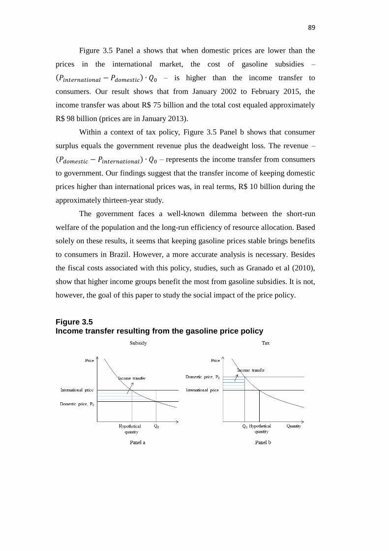
89
Figure 3.5 Panel a shows that when domestic prices are lower than the
prices in the international market, the cost of gasoline subsidies –
(𝑃𝑖𝑛𝑡𝑒𝑟𝑛𝑎𝑡𝑖𝑜𝑛𝑎𝑙 − 𝑃𝑑𝑜𝑚𝑒𝑠𝑡𝑖𝑐) ∙ 𝑄0 – is higher than the income transfer to
consumers. Our result shows that from January 2002 to February 2015, the
income transfer was about R$ 75 billion and the total cost equaled approximately
R$ 98 billion (prices are in January 2013).
Within a context of tax policy, Figure 3.5 Panel b shows that consumer
surplus equals the government revenue plus the deadweight loss. The revenue –
(𝑃𝑑𝑜𝑚𝑒𝑠𝑡𝑖𝑐 − 𝑃𝑖𝑛𝑡𝑒𝑟𝑛𝑎𝑡𝑖𝑜𝑛𝑎𝑙) ∙ 𝑄0 – represents the income transfer from consumers
to government. Our findings suggest that the transfer income of keeping domestic
prices higher than international prices was, in real terms, R$ 10 billion during the
approximately thirteen-year study.
The government faces a well-known dilemma between the short-run
welfare of the population and the long-run efficiency of resource allocation. Based
solely on these results, it seems that keeping gasoline prices stable brings benefits
to consumers in Brazil. However, a more accurate analysis is necessary. Besides
the fiscal costs associated with this policy, studies, such as Granado et al (2010),
show that higher income groups benefit the most from gasoline subsidies. It is not,
however, the goal of this paper to study the social impact of the price policy.
Figure 3.5 Income transfer resulting from the gasoline price policy

90
3.4 Efficiency losses caused by gasoline price distortion
There is a consensus among researchers that government intervention is
sometimes needed to overcome market failures, such as the presence of
externalities. Fossil fuel markets – gasoline and diesel – are examples of goods
that generate negative externalities. Studies such as Parry and Small (2005)
calculate the second-best optimal gasoline tax. They find that gasoline tax in the
United States should be US$ 1.01 per gallon and, in the United Kingdom, US$
1.34 per gallon. While in developed countries government intervention has
increased fuel prices to incorporate external costs, gasoline and diesel are
subsidized in most developing countries. According to the International Energy
Agency (2013), the global cost of fossil-fuel subsidies expanded to $ 544 billion
in 2012 despite efforts at reform.
Davis (2014) examines global fuel subsidies and finds that subsidies for
gasoline and diesel totaled $ 110 billion in 2012 (approximately, R$ 215 billion).
Assuming that demand is described by a constant elasticity demand function with
a time-varying scale parameter and supply is perfectly elastic, Davis (2014)
calculates the deadweight loss. He finds that the total deadweight loss worldwide
equaled $ 44 billion in 2012 (about R$ 86 billion). When incorporating external
costs, such as an increase in CO2 emissions, the economic loss increases
substantially.61
To quantify the deadweight loss created by the gasoline pricing policy in
Brazil, we follow Davis (2014) and assume that the demand for gasoline is
described using a constant elasticity demand function with a time-varying scale
parameter and that the supply is perfectly elastic – Petrobras must attend demand
regardless the price.
Under these hypotheses, the deadweight loss results from a misallocation
of consumption. If supply were positively inclined, then besides consumption
misallocation there would also be a production distortion. In this case, the loss
would be larger than the first one. In this sense, our analysis can be seen as a
lower bound to the deadweight loss calculation.
61
Prices are in 2012.

91
We also assume four additional hypotheses. First, we do not take into
account the externalities generated by gasoline consumption. Second, no other
market failure (such as imperfect competition in the distribution market) is
considered. Third, the analysis is a partial equilibrium one in the sense that no
other fuel market is modeled. And fourth, we assume that there is no storage in the
gasoline market. These simplifying hypotheses allow us to understand the
mechanisms and effects of the stability pricing policy on the gasoline market with
more analytical transparency. After showing the main results, we discuss the
likely biases introduced by each of these hypotheses.
The demand for gasoline is described as:
𝐷𝑔𝑎𝑠𝑜𝑙𝑖𝑛𝑒𝑡= 𝐴𝑡 ∙ 𝑃𝑔𝑎𝑠𝑜𝑙𝑖𝑛𝑒𝑡
𝜖1 ∙ 𝑃𝑒𝑡ℎ𝑎𝑛𝑜𝑙𝜖2 , 𝑡 = January 2002 to February 2015 Eq. 1
Where 𝐷𝑔𝑎𝑠𝑜𝑙𝑖𝑛𝑒 is the quantity of gasoline sold in time 𝑡, 𝐴 is the scale
parameter in 𝑡, 𝑃𝑔𝑎𝑠𝑜𝑙𝑖𝑛𝑒 and 𝑃𝑒𝑡ℎ𝑎𝑛𝑜𝑙 is the gasoline and ethanol prices in 𝑡, and 𝜖
is the long run price elasticity of demand. 62
A critical point in our analysis concerns the long run own- and cross-price
elasticity of gasoline demand. The price policy determines the price of gasoline
sold by the refiners (Petrobras) to the distributors, but we are ultimately interested
on the impact of government intervention on consumers. So, we assume that
distributors behave competitively, so that the price faced by consumers is simply
the price paid by distributors plus a constant distribution cost. Under this
assumption, we ignore the distribution market and use the price-elasticity of
gasoline demand of consumers.
The price of ethanol is the retail price. The difference between the
(𝑝𝑒𝑡ℎ𝑎𝑛𝑜𝑙 – 𝑝𝑔𝑎𝑠𝑜𝑙𝑖𝑛𝑒(𝑤ℎ𝑜𝑙𝑒𝑠𝑎𝑙𝑒)) and the (𝑝𝑒𝑡ℎ𝑎𝑛𝑜𝑙 – 𝑝𝑔𝑎𝑠𝑜𝑙𝑖𝑛𝑒(𝑟𝑒𝑡𝑎𝑖𝑙)) is,
approximately, constant over the time. Therefore, as we are interested in
percentage changes, we use the retail price of ethanol even though we are using
the wholesale price of gasoline.
The magnitude of the deadweight loss depends on the elasticity of the
gasoline demand. In the first chapter of this thesis, we estimate the long-run own-
62
Although we use the long run elasticity, we are not taking into account the extensive margin.
This study focuses on the intensive margin.

92
and cross-price elasticity of gasoline demand to be -1.6 and 0.8. We use these
values to calibrate the scale parameter and, then, to calculate the deadweight loss.
To calculate the scale parameter, we use the amount of gasoline sold by
distributors and the domestic prices of gasoline and ethanol. The distributors buy
gasoline produced or imported by the refineries. But, regardless gasoline origin
(local or imported), the price paid by the distributors is determined by Petrobras.
For example, in January 2002, the cost of gasoline to distributors in
nominal terms was R$ 0.413 per liter.63
For the same period, Brazilians consumed
1,921 millions of liters of gasoline. If we substitute these values in the demand
function (Equation 1) and rearrange it, we are able to determine the scale
parameter. In this case, 𝐴 is approximately 426. This information, along with the
gasoline price in the spot market, allows us to calculate the hypothetical
consumption in Brazil if domestic prices were equal to international prices.64
From January 2002 to February 2015, the price stability policy worked
either as a subsidy or a tax. Most of the time (68%), the gasoline price policy
implemented by Petrobras can be viewed as a subsidy. Although both policies –
subsidy and tax – generate deadweight loss, it is important to distinguish them to
precisely estimate the economic loss of each policy.
Figure 3.6 The economic cost of gasoline price policy
63
This price does not include tax. 64
As gasoline price is determined internationally reflecting global demand and supply conditions,
all (free) countries face similar import and export gasoline prices. Within this context, we should
expect that, without government intervention, prices converge. Otherwise, countries, or
companies, could arbitrage. Of course, national taxation of gasoline and distribution costs differs
among countries and cause significant price differences, but still some convergence might be
expected.

93
Figure 3.6 depicts graphically the efficiency loss generated by the pricing
policy adopted by Petrobras. The stability pricing policy creates a wedge between
the international and the domestic gasoline prices and, consequently, implies in an
inefficiency allocation of resources. To estimate the loss generated by each policy,
we calculate the shaded are in Figure 3.6 Panels a and b.
In Panel a, the deadweight loss occurred because domestic prices are lower
than the price of gasoline in the international market. In this case, the consumption
of gasoline is higher than the optimal consumption. To calculate the efficiency
loss from this allocation, we calculate the shaded area in Panel a.
𝐷𝑊𝐿𝑠𝑢𝑏𝑠𝑖𝑑𝑦 = (𝑃𝑔𝑖𝑛𝑡𝑒𝑟𝑛𝑎𝑡𝑖𝑜𝑛𝑎𝑙− 𝑃𝑔𝑑𝑜𝑚𝑒𝑠𝑡𝑖𝑐
) ∙ 𝑄0 − ∫ 𝐴 ∙ 𝑝𝑔𝜖1 ∙ 𝑝𝑒
𝜖2𝑑𝑝𝑔
𝑃𝑔𝑖𝑛𝑡𝑒𝑟𝑛𝑎𝑡𝑖𝑜𝑛𝑎𝑙
𝑃𝑔𝑑𝑜𝑚𝑒𝑠𝑡𝑖𝑐
𝐷𝑊𝐿𝑠𝑢𝑏𝑠𝑖𝑑𝑦 = (𝑃𝑔𝑖𝑛𝑡𝑒𝑟𝑛𝑎𝑡𝑖𝑜𝑛𝑎𝑙− 𝑃𝑔𝑑𝑜𝑚𝑒𝑠𝑡𝑖𝑐
) ∙ 𝑄0 −𝐴 ∙ 𝑃𝑒
𝜖2
(1 + 𝜖1)∙ (𝑃𝑔𝑖𝑛𝑡𝑒𝑟𝑛𝑎𝑡𝑖𝑜𝑛𝑎𝑙
(1+𝜖1) − 𝑃𝑔𝑑𝑜𝑚𝑒𝑠𝑡𝑖𝑐
(1+𝜖1) )
Panel b shows the economic loss from having domestic prices higher than
international prices. In this situation, the optimal consumption – hypothetical
quantity – is higher than the actual consumption. The deadweight loss is
calculated as the shaded are in Panel b.
𝐷𝑊𝐿𝑡𝑎𝑥 = ∫ 𝐴 ∙ 𝑝𝑔𝜖1 ∙ 𝑝𝑒
𝜖2𝑑𝑝𝑔
𝑃𝑔𝑑𝑜𝑚𝑒𝑠𝑡𝑖𝑐
𝑃𝑔𝑖𝑛𝑡𝑒𝑟𝑛𝑎𝑡𝑖𝑜𝑛𝑎𝑙
− (𝑃𝑔𝑑𝑜𝑚𝑒𝑠𝑡𝑖𝑐− 𝑃𝑔𝑖𝑛𝑡𝑒𝑟𝑛𝑎𝑡𝑖𝑜𝑛𝑎𝑙
) ∙ 𝑄0
𝐷𝑊𝐿𝑡𝑎𝑥 =𝐴 ∙ 𝑃𝑒
∈2
(1 + 𝜖1)∙ (𝑃𝑔𝑑𝑜𝑚𝑒𝑠𝑡𝑖𝑐
(1+𝜖1) − 𝑃𝑔𝑖𝑛𝑡𝑒𝑟𝑛𝑎𝑡𝑖𝑜𝑛𝑎𝑙
(1+𝜖1) ) − (𝑃𝑔𝑑𝑜𝑚𝑒𝑠𝑡𝑖𝑐− 𝑃𝑔𝑖𝑛𝑡𝑒𝑟𝑛𝑎𝑡𝑖𝑜𝑛𝑎𝑙
) ∙ 𝑄0
Under the assumptions about demand and supply stated above, we
calculate the consumption of gasoline under the international and domestic price
(Figure 3.7). As most of the time the price stability policy worked as a subsidy
policy, it led to an overconsumption of gasoline throughout this period. The total
deadweight loss created by the Brazilian stability policy was, from January 2002
to February 2015, R$ 24 billion (prices are in January 2013). As expected, this
economic loss is not constant during the years. While in 2009, the loss equaled R$
218 million, in 2012, the loss was approximately R$ 4 billion (Table 3.1).

94
Figure 3.7 Gasoline consumption (in liters)
Note: To obtain the hypothetical consumption of gasoline in the alternative scenario, we construct
a counterfactual where the price of gasoline in Brazil equals the price of gasoline in the
international market. Also, using a constant elasticity demand function with a time-varying scale
parameter and an estimate of the long-run price elasticity of gasoline demand, we are able to
obtain the hypothetical consumption of gasoline.
The relative magnitude of deadweight loss in 2012 in the gasoline market
in Brazil compares to Indonesia (R$ 4.2 billion in 2012) and Iran (R$ 3.9 billion
in 2012). According to Davis (2014), Venezuela and Saudi Arabia are the top two
countries in terms of gasoline subsidy policy. In 2012, the deadweight loss in
those countries were, approximately, R$ 15 and R$ 10 billion respectively.
It is worth mentioning that the magnitude of the consumption inefficiency
generated by the price policy depends on the elasticity of demand. If we assume
that all market variables are held constant, then a higher elasticity leads to a larger
loss.
0.0
1.0
2.0
3.0
4.0
5.0
6.0
7.0Ja
n-0
2
Jul-
02
Jan
-03
Jul-
03
Jan
-04
Jul-
04
Jan
-05
Jul-
05
Jan
-06
Jul-
06
Jan
-07
Jul-
07
Jan
-08
Jul-
08
Jan
-09
Jul-
09
Jan
-10
Jul-
10
Jan
-11
Jul-
11
Jan
-12
Jul-
12
Jan
-13
Jul-
13
Jan
-14
Jul-
14
Jan
-15
Bil
lion
Baseline scenario Alternative scenario

95
Table 3.1 Deadweight loss from the gasoline price stability policy in Brazil
Deadweight loss
(in million Reais)
Gasoline consumption
(in million liters)
Average gasoline prices (R$
per liter)
Domestic International
2002 419.604 22,610 1.114 1.068
2003 603.402 21,790 1.322 1.192
2004 2.071.184 23,173 1.099 1.417
2005 2.612.017 23,553 1.089 1.489
2006 1.855.690 24,007 1.156 1.477
2007 1.063.528 24,325 1.181 1.414
2008 2.757.883 25,174 1.161 1.475
2009 218.344 25,409 1.071 1.033
2010 262.252 29,843 1.026 1.111
2011 1.281.388 35,491 1.103 1.325
2012 4.120.047 39,697 1.086 1.503
2013 3.589.331 41,426 1.084 1.499
2014 3.405.109 44,364 1.100 1.412
Jan-Feb 2015 353.972 6,970 1.043 0.912
Note: All prices are in January 2013 Brazilian Reais.
Discussion: implications of our model hypotheses
We made four simplifying hypotheses to better understand the
mechanisms and effects of the pricing policy on the gasoline market with more
analytical transparency.
The first assumption concerns the externalities associated with the use of
gasoline. It is well stablished in the literature that the use of gasoline generates
negative externalities such as local and global pollution. Parry, Walls and
Harrington (2007) calculate the extra cost of gasoline due to local and global air
pollution, oil dependency, traffic congestion and traffic accidents, as well as other
externalities. They find that gasoline-related externalities65
add 18 cents per gallon
while mileage-related externalities66
are equivalent to $ 2.10 per gallon. Thus,
incorporating the external costs associated with the use of gasoline leads to a
higher social cost than the one estimated in this paper – where we focus solely on
the deadweight loss resulting from the price stability policy. As the price policy
65
Greenhouse warming and oil dependency. 66
Congestion, accidents and local and global pollution.

96
during the almost thirteen-year study was primarily a subsidy policy, our
estimates can be thought as a lower bound for the economic cost of the
government intervention in the gasoline market.
The second hypothesis is of no other market failure, such as imperfect
competition in the gasoline market. This assumption is controversial. Petrobras
holds a dominant position in the fuel market in Brazil. It is responsible for 98% of
Brazilian refining capacity and it is the leader in the distribution of oil products
and biofuel. The liberalization process in the crude oil industry started in 1995,67
but high logistic costs, bureaucracy, and political interventions discourage
potential entrants from entering in the gasoline market.68
Within this context, Petrobras faces little competition. But, contrary to
private monopolists that maximize profits, the goals of Petrobras are less well
known. Decisions about production and fuel prices are based not only on market
conditions, but also on (short-term) social and political interests. Within this
scenario, an intervention in the gasoline market, such as the price stability
policy,69
leads potentially to an increase in the market concentration, and,
consequently, to economic inefficiency.
Regarding the partial equilibrium analysis assumption, the problem by
holding prices and quantities of other goods fixed is that we ignore the possibility
that events in the gasoline market affect other markets' equilibrium prices and
quantities. When calculating the deadweight loss, for example, we do not take into
account the direct impacts of the price stability policy on the consumption of
ethanol – the closest substitute to gasoline. The control of the price of gasoline
decreases the competitiveness between both fuels and, therefore, potentially leads
to a welfare loss larger than the one estimated under this hypothesis.
Finally, we assume that there is no storage. Under this assumption,
producers cannot arbitrage with price. If arbitrage were allowed, then we would
have to incorporate dynamic elements in our analysis. This assumption is in
accordance with the Brazilian market structure. Petrobras does not have regulatory
storage. In cases where domestic demand for gasoline is less than the production
67
Ninth Constitutional Amendment: new wording to Article 177 of the Federal Constitution. 68
The retail segment is an exception in the oil industry in Brazil. Although there are few gasoline
cartels, the segment is competitive. 69
Because of the monopoly of Petrobras and the stability of the price of gasoline, two major oil
companies, Exxon and Chevron, left the distribution segment in Brazil (Freitas (2011)).

97
of gasoline, Petrobras exports the surplus. When the opposite happens, Petrobras
imports gasoline. It must attend domestic demand.
3.5
Price stability and CO2 emissions
3.5.1
Calculating CO2 emissions
To estimate the impact of Brazilian policy to ensure stable gasoline prices
on CO2 emissions, we follow two steps. First, we calculate CO2 emissions from
gasoline used in Brazil. Different from most countries, the gasoline sold in Brazil
contains 20% to 25% of anhydrous ethanol. And, second, we calculate CO2
emissions based on total consumption of gasoline obtained from ANP and from
the alternative scenario, in which the price of gasoline is set equal to the price of
gasoline in the spot market.
According to the International Energy Agency (IEA), CO2 emissions from
conventional gasoline is 2.8 Kg per liter and from ethanol from sugar cane is as
low as 0.3 Kg per liter.70
If we assume that gasoline contains 25% of ethanol, then
the amount of CO2 emitted by the use of gasoline in Brazil equals 2.175 Kg per
liter.71
3.5.2 CO2 emissions estimates
Larsen and Shah (1992) show that removing world energy subsidies –
more than $ 230 billion – could reduce global carbon emissions by 9%. Also, they
find that the welfare costs of these subsidies are more than $ 20 billion even
without including the negative environmental externalities.
More recently, according to the IPCC report, Climate Change 2014, CO2
emissions from fossil fuel reached 32 billion tons in 2010 and grew further by
70
For many researchers (EPE, 2005), CO2 emissions from ethanol is 0. The amount of CO2
emitted during combustion is compensated by the absorption of this gas through photosynthesis.
However, during production, fossil resources, such as diesel, are used and this must be taken into
account. 71
0.25 ∗ 0.3 + 0.75 ∗ 2.8 = 2.175.

98
about 3% between 2010 and 2011, and by about 1% to 2% between 2011 and
2012.
Figure 3.8 shows the emission of CO2 from January 2002 to February
2015. As expected, CO2 emissions under the baseline scenario are higher than
CO2 emissions under the alternative scenario. This is because the policy to ensure
price stability led, most of the time, to an overconsumption of gasoline.
Throughout the period, total CO2 emissions equaled 798.90 million tons. If the
price of gasoline were equal to the price of gasoline in the international market,
then total CO2 emissions would be 618.58 million tons during the same period. As
a result, the policy to maintain the price of gasoline stable led to an increase in
CO2 emissions of 180.32 million tons – or 29% – during the thirteen-year period.
Figure 3.8 CO2 emissions resulting from the gasoline pricing policy in Brazil
The estimates found here are in accordance with other studies. In 2005, for
example, we find that CO2 emissions from gasoline were 51 million tons for 23
billion liters of gasoline consumed. According to EPE – the Brazilian federal
energy planning company – for the same year, CO2 emissions were 52 million
tons.72
72
To calculate CO2 emissions, EPE uses the gasoline E25 – 25% of anhydrous ethanol and 75% of
gasoline.
-
2
4
6
8
10
12
14
16
Jan
-02
Jul-
02
Jan
-03
Jul-
03
Jan
-04
Jul-
04
Jan
-05
Jul-
05
Jan
-06
Jul-
06
Jan
-07
Jul-
07
Jan
-08
Jul-
08
Jan
-09
Jul-
09
Jan
-10
Jul-
10
Jan
-11
Jul-
11
Jan
-12
Jul-
12
Jan
-13
Jul-
13
Jan
-14
Jul-
14
Jan
-15
Mil
lion t
ons
Baseline scenario Alternative scenario

99
More recently, Gazzoni (2012) finds that, in 2011, total CO2 emissions
from conventional gasoline73
in Brazil were, approximately, 70 million tons. For
the same year, our estimates for CO2 emissions are about 77 million tons.
According to the Ministry of Mines and Energy (MME), total CO2
emissions in Brazil equaled 440 million tons in 2012. Based on our estimates,
total CO2 emissions from gasoline equaled 86 million tons in 2012, i.e., 19% of
total CO2 emissions in Brazil.
3.6
The effects of price stability on the consumption of ethanol
Studies on the effect of fossil fuel subsidies on the ethanol market are
more limited. Besides, most studies are qualitative rather than quantitative. Market
analysts agree that controlling the price of gasoline decreases the competitiveness
between gasoline and ethanol and leads to allocative distortions in both markets.
Different from most countries, fuel market in Brazil is characterized by the
existence of a close substitute to gasoline: ethanol. Consumers, when filling their
automobiles, can choose between gasoline, ethanol or any mix between both fuels.
In the first chapter of this thesis, we show that, from January 2002 to January
2013, the cross-price elasticity of the demand for gasoline is, approximately, 0.8,
suggesting a high degree of substitutability between gasoline and ethanol.
In the first chapter, we focused our analysis on the gasoline market and,
therefore, we did not estimate the demand for ethanol. To calculate the effects of
changes in the price of gasoline on the ethanol market, we need the cross-price
elasticity of ethanol demand. If there were no income effect, then we could use
our previous estimate to obtain the cross-price elasticity. However, we believe this
is a too strong assumption for the fuel market. Therefore, we use the estimate
from Santos (2013).74
Using a dynamic panel data approach, Santos (2013) suggests that the
short-run75
cross-price elasticity of ethanol demand is 1.182. So, a change of 1%
73
Gasoline without the addition of ethanol anhydrous. 74
Santos (2013) is the paper closest to our first paper. 75
To analyze the effect of the pricing policy in Brazil on the ethanol market, we use the short-run
elasticity. Deciding whether to fill the automobile with gasoline or ethanol (or any combination
between both fuels) is a short and not a long run decision.

100
in the price of gasoline leads to an increase of 1.182% in the demand for ethanol.
Adopting this value and under the assumptions about gasoline demand and supply
elasticities, we are able to calculate the consumption of ethanol under an
alternative scenario, where the price of gasoline in Brazil equals the price of
gasoline in the international market.
Figure 3.9 shows ethanol consumption under both scenarios – the baseline
and the alternative one – from January 2002 to February 2015. Under the
alternative scenario, ethanol consumption is higher than under the baseline
scenario, which may imply that the price policy to maintain the price of gasoline
stable has indeed an impact over the ethanol market. Our results suggest that
during the thirteen-year period, ethanol consumption should have been –
considering all other economic variables constant, except for the price of gasoline
–, approximately 142 billion liters instead of 116 billion liters, an increase of 22%.
Figure 3.9 Ethanol consumption under the baseline and the alternative scenarios (in liters)
Notes: the baseline scenario correspond to the current situation, where domestic prices diverge
from the prices in the international market. Under the alternative scenario, we assume that the
domestic price of gasoline equals the price of gasoline in the international market. Also, to obtain
the ethanol consumption under the alternative scenario, we use an estimate for the cross-price
elasticity of ethanol demand found in the literature.
If we assume that the demand for fuel is inelastic, then the difference
between the consumption of ethanol under both scenarios, approximately 25
0.0
0.5
1.0
1.5
2.0
2.5
Jan
-02
Jul-
02
Jan
-03
Jul-
03
Jan
-04
Jul-
04
Jan
-05
Jul-
05
Jan
-06
Jul-
06
Jan
-07
Jul-
07
Jan
-08
Jul-
08
Jan
-09
Jul-
09
Jan
-10
Jul-
10
Jan
-11
Jul-
11
Jan
-12
Jul-
12
Jan
-13
Jul-
13
Jan
-14
Jul-
14
Jan
-15
Bil
lion
Baseline scenario Alternative scenario

101
billion liters, should be allocated to the gasoline market. In this case, the
consumption of gasoline should have increased about 20 billion liters.76
However,
we calculated that the overconsumption of gasoline due to the price policy was 60
billion liters. Therefore, the difference between these two values is not explained
by the impact of the price policy solely on the ethanol market.
Studies such as Klier and Linn (2010) and Busse, Knittel and Zettelmeyer
(2013) show that changes in the price of gasoline affect not only the intensive
margin, but also the extensive margin. Thus, it is possible that the policy to ensure
stable prices of gasoline stimulates automobiles sales in Brazil. More study,
however, is needed in this area to validate (or not) this assumption.
3.7
Conclusion
To measure the impact of the gasoline price policy in Brazil, we
constructed an alternative scenario where the price of gasoline in Brazil equals the
price of gasoline in the spot market. Under additional demand and supply
assumptions, we measured the income transfer, the deadweight loss and the
effects of this policy on the emission of CO2 and the consumption of ethanol.
Our study suggests that the total cost of this policy during the
approximately thirteen-year study was R$ 88 billion. From January 2002 to
February 2015, income transfer to consumers equaled R$ 75 billion and the
deadweight loss R$ 24 billion.77
Under the baseline scenario, while CO2 emissions
were 29% higher than in the alternative scenario, the consumption of ethanol was
18% lower.
All in all, our findings show that the fiscal and environmental costs of this
policy are substantial.78
Brazilian government should allow the pass-through of
international prices to domestic prices to promote efficiency and to mitigate the
impact on the balance of payments, as well as negative externalities.
76
According to the National Institute of Metrology, Quality and Technology in Brazil, 1 liter of
ethanol is equivalent to 0.78 liter of gasoline. 77
All prices are in January 2013. 78
Petrobras – the state-owned oil company – absorbs most of the losses associated with the
gasoline price policy.

102
APPENDIX A3
The pass-through of the price of gasoline to inflation rate
The literature on exchange rate pass-through is vast. We focus on the pass-
through of commodity prices to domestic price inflation. De Gregorio,
Landerretche, and Neilson (2008) present evidence of a decline in the pass-
through of the price of crude oil to the inflation rate during recent decades. To
calculate the pass-through, they use rolling vector autoregression estimations. In a
sample of 34 countries, they find that the fall in the pass-through is more
pronounced in industrial than in emerging economies. According to them, the
reduction in the oil intensity of economies around the world, the reduction in the
exchange rate pass-through, and a more favorable inflation environment are the
most important factors for explaining the declining in the pass-through.
Zoli (2009) shows that shock in commodity prices have a significant
impact on domestic inflation. The inflation response, however, is asymmetric for
positive and negative shocks. Using a panel model for 18 European emerging
economies, with quarterly data, Zoli (2009) finds that, on average, in the long run,
a 1 percentage point surge in oil price inflation leads to an increase in headline
inflation by 0.02 percentage points, whereas a decline in oil price inflation by the
same amount results in a drop in headline inflation by 0.04.
Gelos and Ustyugova (2012) show that countries respond different to
commodity price shocks. In a sample of 25 countries and using several
approaches, they find that economies with higher food shares in the Consumer
Price Index baskets, fuel intensities, and pre-existing inflation levels were more
prone to experience sustained inflationary effects from commodity price shocks.
In Brazil, De Melo (2010) presents evidence that shocks in the
international prices of commodities after June 2005 have a lower impact on
inflation rate. While from January 2000 to May 2005, the pass-through of a 1%
shock in commodity prices on inflation rate equaled, approximately, 30%, from
June 2005 to May 2010, the pass-through was almost null 3 years after the shock.
Ono (2014) shows that an increase of 10% in the price of commodities increases
the inflation rate in 0.132% ten months after the shock. He uses vector

103
autoregression models and database from January 2004 to April 2013 to calculate
the pass-though.
Following the literature on the effects of changes in the exchange rate on
the economy, we use vector autoregressions with exogenous variables (VARX) to
calculate the gasoline price pass-through to the inflation rate in Brazil. Besides the
price of the gasoline to consumers and the inflation rate, we consider the price of
crude oil, the exchange rate and the industrial production index – a measure of
economic activity. These macroeconomic variables are added in the model to
control for potential correlation between these variables and the price of gasoline
and the inflation rate. The reduced-form of the model is:
𝑌𝑡 = Λ0 + Λ1𝑌𝑡−1 + ⋯+ Λ𝑝𝑌𝑡−𝑝 + Θ𝑋𝑡 + 휀𝑡
Where 𝑌 is a vector with the endogenous variables, i.e., the nominal
exchange rate, the industrial production index, the nominal price of gasoline to
consumers and the inflation rate; 𝑋 is the vector with the exogenous variables, i.e.,
the nominal price of crude oil, 11 monthly dummy variables and 2 annual
dummies, 2002 and 2008 to capture the presidential election in Brazil and the
international financial crises respectively; and 𝑝 is the optimal number of lags.
When estimating the VAR model, we transform the variables,79
using the
first-difference of the natural log of the variables to obtain stationarity.80
More specifically, to identify our model and capture the pass-through of
gasoline price to inflation, we assume that the price of crude oil is an exogenous
variable. The price of crude oil is determined in the spot market as a function of,
mainly, global demand and supply. Despite the recent discoveries and the
development of large crude oil and gas reserves, Brazil is not yet a major player in
the crude oil market.
The exchange rate, the industrial production index, the price of the
gasoline, and the inflation rate are assumed to be endogenous variables. To obtain
the causal relationship between them, we assume a recursive chain of causality
among the shocks (or innovations) of these four variables. First, we assume that
79
Except for the inflation rate that is already stationary. 80
Except for the inflation rate, we use the variables in log to obtain the percent variation when
taking the first-difference.

104
the exchange rate is affected contemporaneously by the shock to itself. According
to Meese and Rogoff (1983) and Cheung, Chinn and Pascual (2005), the exchange
rate is better explained by a random walk than by more complex models.81
Without being too restrictive, we allow that the past values of the other
macroeconomic variables used in this study offer improvement in forecasting
exchange rate movements. Second, we assume that industrial production is not
affected contemporaneously by shocks in the gasoline market and in the inflation
rate.82
Third, we allow that the price of gasoline be affected contemporaneously
by the economic activity. It is plausible to think that when the economy increases,
the income also increases and, as a result, people drive more, using, therefore,
more gasoline. And, fourth, we assume that the inflation rate may respond to
contemporaneous changes in the exchange rate, the economic activity and the
gasoline price.
In matrix notation, those assumptions imply that the reduced-form vectors
– 휀– are related to the shocks (structural disturbances) – 𝑢 – in the following way:
[
1 0 0 0∅21 1 0 0∅31 ∅32 1 0∅41 ∅42 ∅043 1
] ∙
[ 휀𝑡
𝑒𝑥𝑐ℎ𝑎𝑛𝑔𝑒 𝑟𝑎𝑡𝑒
휀𝑡𝑖𝑛𝑑𝑢𝑠𝑡𝑟𝑖𝑎𝑙 𝑝𝑟𝑜𝑑𝑢𝑐𝑡𝑖𝑜𝑛
휀𝑡𝑔𝑎𝑠𝑜𝑙𝑖𝑛𝑒 𝑝𝑟𝑖𝑐𝑒
휀𝑡𝑖𝑛𝑓𝑙𝑎𝑡𝑖𝑜𝑛 𝑟𝑎𝑡𝑒
]
=
[ 𝑢𝑡
𝑒𝑥𝑐ℎ𝑎𝑛𝑔𝑒 𝑟𝑎𝑡𝑒
𝑢𝑡𝑖𝑛𝑑𝑢𝑠𝑡𝑟𝑖𝑎𝑙 𝑝𝑟𝑜𝑑𝑢𝑐𝑡𝑖𝑜𝑛
𝑢𝑡𝑔𝑎𝑠𝑜𝑙𝑖𝑛𝑒 𝑝𝑟𝑖𝑐𝑒
𝑢𝑡𝑖𝑛𝑓𝑙𝑎𝑡𝑖𝑜𝑛 𝑟𝑎𝑡𝑒
]
All in all, to identify our model and to calculate impulse response
functions, we assume that the errors are orthogonalized using the Cholesky
decomposition. To obtain the pass-through we calculate the accumulated impulse
response functions. Following the literature on exchange rate pass-through, we
use the ratio between the accumulated responses of inflation rate to one standard
deviation shock 𝑗 horizons after the shock to measure the gasoline pass-through to
inflation.83
81
Knowing the determinants of the exchange rate is still an active area of research. 82
We assume that the common shocks between the price of gasoline and the industrial production
that could bias our estimates are the shocks in the crude oil market and in the exchange rate; both
shocks are taking into account in our model. 83
After estimating the VAR model, we conduct several tests (shown in Appendix 1) to ensure that
the model captures well the dynamics between the variables.

105
Figure A3.1 displays the response and the accumulated response of the
inflation rate to a one-standard deviation shock in the price of gasoline.84,85
The
dashed lines in Figure A3.1 represent the two standard deviation confidence
intervals, which are calculated using Monte Carlo simulations with 1,000
replications. The impulse response in Figure A3.1 suggests that an increase of one
standard deviation (about 5.22%) in the price of gasoline leads to an instantaneous
increase of 0.14% in the inflation rate. It is worth mentioning that as the inflation
rate is not in log, the increase is additive. So, for example, if the monthly inflation
rate in January 2013 is 0.86%, then, within a context where everything else is
constant except for the shock in the price of gasoline, the monthly inflation rate in
February 2013 would be 1%, an increase of approximately 16%.
The accumulated impulse response in Figure A3.1 suggests that six
months after the shock, the accumulated response is 0.29% and after one year,
0.3%. As mention before, we can interpret this change as percentage points, so,
within a scenario where we forecast an annual inflation equal to 6%, we should,
after the gasoline price shock, adjust our forecast to 6.3%.
Based on the exchange rate pass-through literature, the pass-through of the
shock in the price of gasoline to inflation rate is 5.74% one year after the one-
standard deviation shock. This pass-through seems small and present evidences
that the government intervention in the gasoline market prevents a higher pass-
through.
84
The accumulated impulse-response functions for the other variables are shown in Appendix A. 85
As the price of gasoline was transformed to log first difference, the one-standard deviation shock
is interpreted as a permanent shock.

106
Figure A3.1 Response of the inflation rate to a one-standard deviation shock in the price of gasoline with two standard error bounds

107
4 References
ACKEBERGE, D.ET AL. Econometric tools for analyzing market outcomes.
In:Handbook of Econometrics 6, 2007, pp. 4171 – 4276.
AGÊNCIA NACIONAL DE PETRÓLEO, GÁS NATURAL E
BIOCOMBUSTÍVEIS.Boletim Anual de Preços 2012: preços do petróleo, gás
natural e combustíveis nos mercados nacional e internacional. ANP, 2012.
ALVES, D. C. O.; BUENO, R. L. S. Short-run, long-run and cross elasticities
of gasoline demand in Brazil. Energy Economics, March 2003, 25, pp. 191-99.
ASSUNÇÃO, J.; PESSOA, J. P.; REZENDE, L. B. Flex Cars and Competition
in Ethanol and Gasoline Retail Markets. CEP Discussion Paper n. 1251,
December 2013. Available at: http://cep.lse.ac.uk/pubs/download/dp1251.pdf.
BALTAGI, B. H.; GRIFFIN, J. M. Gasoline demand in the OECD: an
application of pooling and testing procedures. European Economic Review,
1983, 22, pp. 117-37.
BARRO, R. P.; CURRY, S.; ULYSSEA, G. A desigualdade de renda no Brasil
encontra-se subestimada? Uma análise comparativa com base na PNAD, na
POF e nas Contas Nacionais. IPEA Working Paper n.1263. March, 2007.
Available at:
http://www.ipea.gov.br/portal/index.php?option=com_content&view=article&id=
4842
BERRY, S.T. Estimating discrete choice-models with product differentiation.
The RAND Journal of Economics, Summer 1994, v. 25, n. 2, pp. 242-62.
BERRY, S.; LEVINSOHN, J. and PAKES, A. Automobile prices in market
equilibrium. Econometrica, July 1995, v. 63, n. 4, pp. 841-90.
________. Association voluntary export restraints on automobiles: evaluating
a trade policy. American Economic Review, June 1999, v.89, n. 3, pp. 400-30.
BRESNAHAM, T. F. Competition and collusion in the American automobile
industry: the 1955 price war. The Journal of Industrial Economics, June 1987, v.
35, n. 4, pp. 457-82.
BURKE, P. J.; NISHITATENO, S. Gasoline prices, gasoline consumption, and
new-vehicle fuel economy: Evidence for a large sample of countries. Energy
Economics, March 2013, 36, pp. 363-70.
BUSSE, M. R.; KNITTEL,C. R. and ZETTELMEYER, F. Are Consumers
Myopic? Evidence from New and Used Car Purchases. American Economic
Review, 2013, 103(1), pp. 220–256.

108
CAMERON, A. C.; GELBACH, J. B.; MILLER, D. L. Bootstrap-Based
Improvements for Inference with Clustered Errors. Review of Economics and
Statistics, August 2008, 90 (3), pp. 414-27.
CAMERON, A. C.; MILLER, D. L. A Practitioner's Guide to Cluster-Robust
Inference. Working paper. 2013.
<http://cameron.econ.ucdavis.edu/research/Cameron_Miller_Cluster_Robust_Oct
ober152013.pdf> cited September, 26 2014.
CHAPOTO, A.; JAYNE, T. S. Do Market Interventions Promote Food Price
Stability? Evidence from Eastern and Southern Africa. CAADP Programme
and Alliance for Commodity Trade in Eastern and Southern Africa conference.
Lusaka, Zambia, May 10, 2010.Available at:
http://fsg.afre.msu.edu/gisama/Session_2-
effects_Market_Interventions_on_Price_Stability-Chapoto.pdf.
CHEUNG, Y-W., CHINN, M. and PASCUAL, A. Empirical Exchange Rate
Models of the Nineties: Are any Fit to Survive? Journal of International Money
and Finance, 2005, 24, pp. 1150-1175.
COLOMER, M.; TAVARES, A. Precificação de Combustíveis no Brasil e as
Barreiras ao Investime nto. Discussion paper IE/UFRJ, October 2012, n. 004.
COYLE, D.; DEBACKER, J.; PRISINZANO, R. Estimating the supply and
demand of gasoline using tax data. Energy Economics, January 2012, 34, pp.
195–200.
DAHL, C. A. Consumer adjustment to a gasoline tax. Review of Economics
and Statistics, August 1979, 63 (3), pp. 427-32.
DAVIDSON, R.; MACKINNON, J. G. Wild bootstrap tests for IV regression.
Journal of Business and Economic Statistics, 2010, 28(1), pp. 128-44.
DAVIS, L. W. The economic cost of global fuel subsidies. American Economic
Review: Papers & Proceedings, 2014, 104 (5), pp. 581-585.
DAVIS, L. W.; KILLIAN, L. Estimating the effect of gasoline tax on carbon
emissions. Journal of Applied Econometrics, November/December 2011, 26, pp.
1187-214.
DE GREGORIO, J.; LANDERRETCHE, O; and NEILSON, C. Another pass-
through bites the dust? Oil price and inflation.Economía, 7 (2), pp. 155–208.
DE MELO, A. C. Análise do impacto dos preços das commodities sobre a
inflação no Brasil. Brasília, 2010, Dissertation – Economics Departmanet
Universidade de Brasília.
DE NEGRI, JOÃO ALBERTO. Elasticidade-renda e elasticidade-preço da
demanda de automóveis no Brasil. IPEA working Paper, April 1998, n.558.

109
DE SOUZA E SILVA, C. M. Estratégia de preços da Petrobras no mercado de
combustíveis brasileiro pós-liberalização e instrumentos de amortecimento de
variações internacionais. Master’s thesis. Universidade Federal do Rio de
Janeiro, 2003.
DE SOUZA, S. A.; PETTERINI, F.C.; MIRO, V. H. A tributação nas vendas de
automóveis no Brasil: quem paga a maior parte da conta? EconomiA,
September/December 2010, v.11, n.3, pp.559–96.
DUBÉ, J-P; FOX, J. T.; SU, C-L. Improving the numerical performance of
static and dynamic aggregate discrete choice random coefficients demand
estimation. Econometrica, September 2012, v. 80, n. 5, pp. 2231–2267.
EMPRESA DE PESQUISA ENERGÉTICA (EPE). Potencial de redução de
emissões de CO2 em projetos de produção e uso de biocombustíveis. Estudos
EPE, 2005.
ENGLE, R. F.; GRANGER, C. W. J. Co-Integration and Error Correction:
Representation, Estimation, and Testing. Econometrica, March 1987, 55 (2),
pp. 251-76.
ESPEY, M. Gasoline demand revisited: an international meta-analysis of
elasticities. Energy Economics, 1998, v. 20, pp. 273-295.
FEDERICO, G., DANIEL, J. A.; BINGHAM, B. Domestic petroleum price
smoothing in developing and transition countries. International Monetary Fund
working paper, 2001, WP/01/75.
FERRAZ, C.; FIUZA, E. P. S.; SEROA DA MOTTA, R.Medindo os efeitos da
regulação ambiental em mercados de oligopólio: o caso da poluição
automotiva.Pesquisa e Planejamento Econômico, December 2001, v. 31, n. 3, p.
333-56.
FREITAS, T. Três empresas dominam quase 70% da distribuição de gasolina.
Folha de São Paulo, São Paulo, 30 de abril de 2011. Available at:
http://www1.folha.uol.com.br/fsp/mercado/me3004201119.htm.
FURLONG K. J. Quantifying the benefits of new products: hybrid vehicles.
Working paper. 2011. <http://www4.ncsu.edu/~kjfurlon/Furlong_Ch_1.pdf> cited
October 2014.
GAZZONI, D. L. Balanço de emissões de dióxido de carbono por
biocombustíveis no Brasil:histórico e perspectivas. Documentos Embrapa Soja,
2012, n. 334.
GELOS, G.; USTYUGOVA, Y. Inflation Responses to Commodity Price
Shocks – How and Why Do Countries Differ? International Monetary Fund
working paper, 2012, WP/12/225.

110
GILLEN, B. J.; SHUM, M.; MOON, H. R. Bayesian Model Comparison.
Emerald Group Publishing Limited, 2014, v. 34, pp. 301-323. ISSN: 0731-
9053/doi:10.1108/S0731-905320140000034020.
GIOVANI, F. S.; GISELE, F. T.; LUIZ A. M. P. The impact of a growing
ethanol market on the demand for gasoline in Brazil. Unpublished manuscript,
2009.
GOLDBERG, P. K. Product differentiation and oligopoly in international
markets: the case of the U.S. automobile industry. Econometrica, July 1995, v.
63, n. 4, pp. 891-951.
HAUSMAN, J. A.; LEONARD, G. K. The competitive effects of a new product
introduction: a case study. The Journal of Industrial Economics, 2002, v. 50, pp.
237-263.
HAVRANEK, T.; IRSOVA, Z.; JANDA, K. Demand for gasoline is more price-
inelastic than commonly thought. Energy Economics, 2012, pp. 201-207.
HOLZ-EAKIN, D.; NEWEY, W.; ROSEN, H. S. Estimating Vector
Autoregressions with Panel Data. Econometrica, November 1988, 56 (6), pp.
1371-95.
HUGHES, J. E.; KNITTEL, C. R.; SPERLING, D. Evidence of a shift in the
short-run price elasticity of gasoline demand. The Energy Journal, 2008, 29 (1),
pp. 93-114.
INMETRO. Gás Natural na Matriz de Combustíveis Veiculares. 2005.
Available at: http://www.inmetro.gov.br/metlegal/palestras/Petrobras.pdf.
INTERGOVERNAMNETAL PANEL ON CLIMATE CHANGE. Climate
change 2014. IPCC Fifth Assessment Report, 2014.
INTERNATIONAL ENERGY AGENCY. IEA Energy Technology Essentials –
Biofuel Production. IEA text base, 2007. Available
at:http://www.iea.org/publications/freepublications/publication/essentials2.pdf.
_______________. CO2 emissions from fuel combustion. IEA statistics, 2013.
_______________. World Energy Outlook 2013. Paris: IEA, 2013.
KLIER, T.; LINN, J. The Price of Gasoline and New Vehicle Fuel Economy:
Evidence from Monthly Sales Data. American Economic Journal: Economic
Policy, 2010, 2 (3), pp. 134–153.
KNITTEL, C. R.; METAXOGLOU, K. Estimation of random-coefficient
demand models: two empiricists’ perspective. Review of Economics and
Statistics, March 2014, v. 96, n. 1, pp. 34–59.
111
LARSEN, B.; SHAH, A. World fossil fuel subsidies and global carbon
emissions. World Bank working paper, 1992.
LIU, W. Modelling gasoline demand in the United States: a flexible
semiparametric approach. Job market paper, State University of New York at
Binghamton, 2011.
LUCINDA, C. R. Quantifying the benefits of multifuel cars: an application of
random-coefficients logit model. FEA Working paper. 2010.
<http://www.fearp.usp.br/pesquisa/images/Anexos/Publicacoes/Textos_discussao/
REC/2010/TD-E01-2010.pdf> cited October 2014.
LUTKEPOHL, H. New introduction to multiple time series analysis. Springer,
2007.
MANZAN, S.; ZEROM, D. A semiparametric analysis of gasoline demand in
the United States reexamining the impact of price. Econometric Reviews,
2010, 29 (4), pp. 439-68.
MEESE, R.; ROGOFF, K. Empirical Exchange Rate Models of the Seventies.
Journal of International Economics, 1983, 14, pp. 3-24.
MINISTÉRIO DE MINAS E ENRGIA. Energia no mundo. 2014. Available at:
http://www.eletronuclear.gov.br/LinkClick.aspx?fileticket=FLeBqE8xTX8%3d&t
abid=69.
MINISTÉRIO DO MEIO AMBIENTE. Inventário nacional de emissões
atmosféricas por veículos automotores rodoviários. 2012. Available at:
http://www.mma.gov.br/images/arquivo/80060/Inventario_de_Emissoes_por_Vei
culos_Rodoviarios_2013.pdf.
NAPPO, M. Demanda por gasolina no Brasil: uma avaliação de suas
elasticidades após a introdução dos carros bicombustíveis. Master’s thesis,
Fundação Getúlio Vargas - EESP, 2007.
NEVO, A. A research assistant’s guide to random coefficients discrete choice
models of demand. NBER Technical Working Paper No. 221. 1998.
<http://www.nber.org/papers/t0221 > cited September 2014.
________.New products, quality changes, and welfare measures from
estimated demand systems. Review of Economics and Statistics, v. 85, pp. 266-
75.
________. Measuring market power in the ready-to-eat cereal industry.
Econometrica, March 2001, v. 69, n. 2, 304-42.
ONO, G. S. Análise do impacto dos preços das commodities sobre a inflação
no Brasil. São Paulo, 2014, 46f. Masters Dissertation – Escola de Economia da
Fundação Getúlio Vargas.

112
PARRY, I. W. H.; SMALL, K. A. Does Britain or the United States Have the
Right Gasoline Tax? American Economic Review, 2005, 95 (4), pp. 1276–89.
PARRY, I. W. H.; WALLS, M.; HARRINGTON, W. Automobile externalities
and policies. Journal of Economic Literature, May 2007, v. 45, n. 2, pp. 373-99.
PESARAN, M. H.; SHIN, Y.; SMITH, R. P. Pooled mean group estimation of
Dynamic heterogeneous panels. August 1997, Working Paper. Available at:
http://www.econ.ed.ac.uk/papers/pmge.pdf
PESARAN, M. H.; SMITH, R. Estimating long-run relationships from
dynamic heterogeneous panels. Journal of Econometrics, 1995, v. 68, pp. 79-
113.
PETRIN, A. Quantifying the benefits of new products: the case of the
Minivan. Journal of Political Economy, 2002, v. 110, n. 4, pp. 705-729.
PETROBRAS. Fact Sheet 2014. Available at:
http://investidorpetrobras.com.br/pt/kit-do-acionista/fact-sheet.htm.
PINTO JR., H. Q (Org). Matriz brasileira de combustíveis. Instituto de
Economia da UFRJ e Núcleo de Assuntos Estratégicos da Presidência da
República, 2006. <http://www.biblioteca.presidencia.gov.br> cited November, 22
2013.
RAMSEY, J.; RAASCHE, R.; ALLEN, B. An analysis of the private and
commercial demand for gasoline. Review of Economics and Statistics,
November 1975, 57 (4), pp. 502-7.
ROPPA, B. Evolução do consumo de gasolina e suas elasticidades: 1973 a
2003. Monograph, Universidade Federal do Rio de Janeiro - UFRJ, 2005.
ROQUE, P. A indústria continua em crise. Agroanalysis, September 2013, pp.
6-8.
SANTOS, G. F. Fuel demand in Brazil in a dynamic panel data approach.
Energy Economics, 2013, 36, pp. 229-40.
SCOTT, K. R. Rational habits in gasoline demand. Energy Economics,
September 2012, 34, pp. 1713-23.
SILVA, G. F.; TIRYAKI, G. F.; PONTES, L. A. M. The impact of a growing
ethanol market on the demand elasticity for gasoline in Brazil. 32nd Annual
International Associationfor Energy Economics Conference, San Francisco, 2009.
SOLOWIEJCZYK, A.; COSTA, R. P. F. O controle de preço da gasolina pode ser
fatal. Agroanalysis, February 2013, pp. 21-22.
STOCK, J. H.; WATSON, M. W. A simple estimator of cointegrating vectors
in higher order integrated systems. Econometric, July 1993, v. 61, pp. 783-820.

113
TRAIN, K. Discrete choice methods with simulation. Cambridge University
Press, September 2009, 2nd edition.
WORLD BANK. State and trends of carbon pricing. May 2014. Available at:
http://www.ecofys.com/files/files/world-bank-ecofys-2014-state-trends-carbon-
pricing.pdf
VILELA, T. M. M; PINTO JR, H. Q. Análise de sensibilidade do consumo de
gasolina C entre julho de 2001 e dezembro de 2008: Política Tributária
Estadual como instrumento de políticas energéticas e ambientais. Nova
Economia, September – December 2010, 20 (3), pp. 403-26.
YATCHEW, A.; NO, J. A. Household gasoline demand in Canada.
Econometrica, November 2011, 69, pp. 1679-1709.
ZETENEYI, K. Vehicle upsizing under the new CAFE standard? An
application of endogenous characteristics choice with fixed. Working paper.
2013.<http://media.wix.com/ugd/c00c41_6255ff1d8274432cad369112feb23062.p
df> cited in November 2014.
ZOLI, E. Commodity Price Volatility, Cyclical Fluctuations, and
Convergence: What is Ahead for Inflation in Emerging Europe? IMF
Working Paper n.41, March 2009.Washington: International Monetary Fund.