arX

iv:1

604.

0375

1v1

[ast

ro-p

h.IM

] 13

Apr

201

6Mon. Not. R. Astron. Soc.000, 1–12 (2012) Printed 5 July 2018 (MN LATEX style file v2.2)

The 154 MHz radio sky observed by the Murchison WidefieldArray: noise, confusion and first source count analyses

T. M. O. Franzen1 ∗, C. A. Jackson1,2, A. R. Offringa3, R. D. Ekers1,2, R. B. Wayth1,2,G. Bernardi4,5,6, J. D. Bowman7, F. Briggs8,2, R. J. Cappallo9, A. A. Deshpande10,B. M. Gaensler11,2,12, L. J. Greenhill6, B. J. Hazelton13, M. Johnston-Hollitt14,D. L. Kaplan15, C. J. Lonsdale9, S. R. McWhirter9, D. A. Mitchell16,2, M. F. Morales13,E. Morgan17, J. Morgan1, D. Oberoi18, S. M. Ord1,2, T. Prabu10, N. Seymour1,N. Udaya Shankar10, K. S. Srivani10, R. Subrahmanyan10,2, S. J. Tingay1,2, C. M. Trott1,2,R. L. Webster19,2, A. Williams1 and C. L. Williams171International Centre for Radio Astronomy Research, CurtinUniversity, Bentley, WA 6102, Australia2ARC Centre of Excellence for All-sky Astrophysics (CAASTRO)3Netherlands Institute for Radio Astronomy (ASTRON), PO Box2, 7990 AA Dwingeloo, The Netherlands4SKA SA, 3rd Floor, The Park, Park Road, Pinelands, 7405, South Africa5Department of Physics and Electronics, Rhodes University,PO Box 94, Grahamstown 6140, South Africa6Harvard-Smithsonian Center for Astrophysics, 60 Garden Street, Cambridge, MA 02138, USA7School of Earth and Space Exploration, Arizona State University, Tempe, AZ 85287, USA8Research School of Astronomy and Astrophysics, AustralianNational University, Canberra, ACT 2611, Australia9MIT Haystack Observatory, Westford, MA 01886, USA10Raman Research Institute, Bangalore 560080, India11Sydney Institute for Astronomy, School of Physics, The University of Sydney, NSW 2006, Australia12Dunlap Institute for Astronomy and Astrophysics, University of Toronto, ON, M5S 3H4, Canada13Department of Physics, University of Washington, Seattle,WA 98195, USA14School of Chemical& Physical Sciences, Victoria University of Wellington, Wellington 6140, New Zealand15Department of Physics, University of Wisconsin–Milwaukee, Milwaukee, WI 53201, USA16CSIRO Astronomy and Space Science (CASS), PO Box 76, Epping,NSW 1710, Australia17Kavli Institute for Astrophysics and Space Research, Massachusetts Institute of Technology, Cambridge, MA 02139, USA18National Centre for Radio Astrophysics, Tata Institute forFundamental Research, Pune 411007, India19School of Physics, The University of Melbourne, Parkville,VIC 3010, Australia

Accepted ????. Received ????

ABSTRACT

We analyse a 154 MHz image made from a 12 h observation with theMurchison Wide-field Array (MWA) to determine the noise contribution and behaviour of the source countsdown to 30 mJy. The MWA image has a bandwidth of 30.72 MHz, a field-of-view within thehalf-power contour of the primary beam of 570 deg2, a resolution of 2.3 arcmin and contains13,458 sources above 5σ. The rms noise in the centre of the image is 4− 5 mJy/beam. TheMWA counts are in excellent agreement with counts from otherinstruments and are the mostprecise ever derived in the flux density range 30–200 mJy due to the sky area covered. Usingthe deepest available source count data, we find that the MWA image is affected by sidelobeconfusion noise at the≈ 3.5 mJy/beam level, due to incompletely-peeled and out-of-imagesources, and classical confusion becomes apparent at≈ 1.7 mJy/beam. This work highlightsthat (i) further improvements in ionospheric calibration and deconvolution imaging techniqueswould be required to probe to the classical confusion limit and (ii) the shape of low-frequencysource counts, including any flattening towards lower flux densities, must be determined fromdeeper≈ 150 MHz surveys as it cannot be directly inferred from higherfrequency data.

Key words: catalogues — galaxies: active — radio continuum: galaxies —surveys

∗Email: thomas.franzen@curtin.edu.auc© 2012 RAS

2 Franzen et al.

1 INTRODUCTION

Radio source counts embody information about the extragalacticsource populations and their evolution (i.e. space density) over cos-mic time as determined by Longair (1966) and many others since.Whilst bright sources are relatively easy to identify, theyare rare;the vast bulk of radio continuum emission emanates from moderateand low-power extragalactic radio sources whose radio emission isdue to a central Active Galactic Nucleus (AGN) and/or ongoing starformation. These sources are distributed over a large rangeof red-shifts, and thus contribute to the source counts to low flux densities.Surveys at a wide range of radio frequencies probe the faint sky, al-though at low frequencies (< 200 MHz), large-area (> 100 deg2)surveys remain limited to confusion effects at the mJy level, mainlydue to large instrumental beam sizes. The situation is expected toimprove with the extensive baselines and sensitivity of theLow Fre-quency Array (LOFAR; van Haarlem et al. 2013) and Square Kilo-metre Array Low (Dewdney et al. 2012), which should push thislimit substantially fainter.

Radio source counts can be used to derive the integrated skybrightness and the power spectrum signature of the extragalacticsources (e.g. Condon et al. 2012; Toffolatti et al. 1998). The typi-cal sensitivity limit to which sources can be reliably extracted froma uniform survey is 5σ, whereσ is due to the combination of con-fusion and system noise. However, even in fairly low resolutionimages where the noise is dominated by classical confusion,sur-vey data can be statistically probed below the 5σ limit using theP(D) (Scheuer 1957) distribution analysis to deduce the probableunderlying source count behaviour (see e.g. Mitchell & Condon1985; Condon et al. 2012). The large field-of-view (FoV) of theMurchison Widefield Array (MWA) and the huge number of de-tected sources gives rise to potential sidelobe confusion in images.Although we know that the deepest MWA images to date are con-fusion limited, therelative contribution of classical and sidelobeconfusion is poorly determined: this makes it hard to statisticallyinterpret survey data below the source detection thresholdand toassess whether enhancements in the data processing, such asim-proved deconvolution techniques, have the potential to further re-duce the noise.

Whilst our science driver is to determine the MWA radiosource counts to probe the contributing extragalactic source popula-tions and their evolution, these data are also important foranalyseswhere these sources are considered contaminating foregrounds. Anumber of new instruments, including the MWA are seeking to de-tect the first global signals from the Epoch of Reionisation (EoR);these rely on direct foreground source subtraction or isolation ofthe composite foreground signal to isolate the much fainterEoRsignal in the power spectra.

MWA EoR observations concentrate on fields selected athigh Galactic latitude free of diffuse Galactic emission. Thereare two options to extracting the EoR signal from the fore-ground signals: (i) via direct foreground subtraction and (ii) viatheir statistical suppression within the power spectrum (see e.g.Morales & Hewitt 2004; Harker et al. 2010; Chapman et al. 2012;Trott, Wayth & Tingay 2012; Parsons et al. 2014). Both methodsbenefit from high-validity source catalogues, and for (ii),a signif-icant extrapolation of the known source counts to model the be-haviour of foreground sources to deep flux density limits to permitmaximal analysis of the power spectrum.

In the absence of the availability of low frequency sourcecounts, their behaviour has been deduced by extrapolating thecounts at 1400 MHz, which are well determined to≈10 µJy. This

approach was used by Thyagarajan et al. (2013a) to estimate thelevel of foreground contamination expected in MWA EoR powerspectra. However, adopting simple spectral index conversions is un-reliable because the shape of the radio source counts changes withfrequency due to the changing nature of the sources contributingto the counts at 1400 and 154 MHz, and the relative dominance of(any) flat-spectrum, beamed component(s) (see e.g. Wall (1994),Jackson & Wall (1999) and references therein).

In this paper, we use an image of one MWA EoR field (EoR0)to determine the 154 MHz source counts down to≈ 30 mJy.We can probe the behaviour of classical and sidelobe confusionnoise atS < 30 mJy by comparing with other source countdata: this approach allows us to determine that the classical con-fusion noise becomes apparent at≈ 1.7 mJy/beam and the sidelobeconfusion noise can be expressed as a Gaussian distributionwithrms ≈ 3.5 mJy/beam. Given that the sidelobe confusion noise islarger than the classical confusion limit, we do not attemptto ex-trapolate the behaviour of the 154 MHz source counts. Instead weinvestigate how sensitive our estimates are to a flattening in thesource count slope below 6 mJy. In conclusion, we discuss likelyorigins of sidelobe confusion in MWA images and areas of futurework.

2 MWA INSTRUMENT AND NOISE CHARACTERISTICS

The MWA is an interferometer comprised of 128 16-crossed-pair-dipole antenna ‘tiles’ distributed over an area≈ 3 km in diameter.It operates at frequencies between 72 and 300 MHz, with an in-stantaneous bandwidth of 30.72 MHz. It is located at the Murchi-son Radio-astronomy Observatory in Western Australia and is thelow-frequency precursor telescope for the SKA. We refer thereaderto Lonsdale et al. (2009) and Tingay et al. (2013) for detailsof thetechnical design and specifications of the MWA. The primary sci-ence objectives of the MWA are detailed in Bowman et al. (2013).Using a uniform image weighting scheme, the angular resolution at154 MHz is approximately 2.5 by 2.2 sec(δ + 26.7◦) arcsec. Giventhe effective width (≈ 4 m) of the MWA’s antenna tiles, the pri-mary beam FWHM is 27◦ at 154 MHz. The excellent snapshotuvcoverage of the MWA, owing to the very large number (8128) ofbaselines, and its huge FoV allow it to rapidly image large areas ofsky.

A key science goal for the MWA is to search for the redshifted21-cm emission from the EoR in the early Universe. Several fieldsare being targeted with deep (accumulating up to 1000 h), pointedobservations (see e.g. Beardsley et al. 2013). The confusion noisein these EoR images is worse than the thermal noise as we show inSection 5, making them ideal for measuring confusion. They alsocover a sufficiently large area of sky to allow the source counts tobe measured accurately over a wide range of flux densities.

There are three contributions to the total noise in all MWAimages: system noise, classical confusion and sidelobe confusion,where we take sidelobe confusion to include calibration errors andsmearing effects. In the remainder of this section, we briefly de-scribe these in context of our current understanding of MWA ob-servations.

2.1 Thermal noise

The Gaussian random noise term,Tsys, is equal toTsky+Trec, whereTsky is the sky noise andTrec the receiver noise. Given the low ob-serving frequency of the MWA,Tsys is dominated byTsky, with a far

c© 2012 RAS, MNRAS000, 1–12

The 154 MHz radio sky observed by the Murchison Widefield Array 3

lower contribution fromTrec. The thermal noise contribution in realMWA data can be estimated using an imaging mode with no con-fusion. StokesV data are ideal providing identical aperture planecoverage and noise characteristics. In a single MWA 2 min snap-shot at high Galactic latitude, for a central frequency of 154 MHzand a bandwidth of 30.72 MHz, the measured rms noise in uni-formly weighted StokesV images is≈ 16 mJy/beam.

From Tingay et al. (2013), in theory, the naturally weightedsensitivity for the same integration time, central frequency andbandwidth is≈ 5 mJy/beam (this assumesTsky = 350 K andTrec = 50 K). After accounting for a 2.1-fold loss in sensitivity dueto uniform weighting (Wayth et al. 2015) and a reduction of≈ 25per cent in the bandwidth due to flagged edge channels, the theo-retical prediction is 2.1√

0.75× 5 mJy/beam≈ 12 mJy/beam, which

compares well with our measurement above.

2.2 Classical confusion

Classical confusion occurs when the surface density of faint extra-galactic sources is high enough to prevent the sources from beingresolved by the array. The fluctuations in the image are due tothesum of all sources in the main lobe of the synthesised beam. Clas-sical confusion only depends on the source counts and the synthe-sised beam area (Condon 1974).

Bernardi et al. (2009) used a power spectrum analysis to es-timate the classical confusion noise in three 6× 6 deg2 sky ar-eas observed with the Westerbork Synthesis Radio Telescopeat150 MHz. They estimated the rms classical confusion noise at150 MHz, σc, to be 3 mJy/beam for a 2 arcmin beam. Otheranalyses to estimate the MWA classical confusion limit haveextrapolated higher frequency source counts given the paucityof deep 150 MHz source count data and have adopted slightlydifferent beam size estimates. Using the method described inThyagarajan et al. (2013a), Thyagarajan (2013b) estimatedσc fromextrapolation of the 1400 MHz counts by Hopkins et al. (2003)to150 MHz. Assumingα1400

150 = −0.78 (S ∝ να) and a source sub-traction limit of 5σ, they obtainedσc = 3 mJy/beam for a 2 ar-cmin beam. Wayth et al. (2015) estimatedσc from extrapolationof the 327 MHz counts measured by Wieringa (1991) down to4 mJy. Following Condon and using a signal-to-noise threshold of6, Wayth et al. obtainedσc = 2 mJy/beam for a 2.4 arcmin beam.

LOFAR EoR observations are probing the 115–190 MHzsky to ≈ 30 µJy/beam rms, although no deep extragalacticsource catalogues are yet available. Observations with theGi-ant Metrewave Radio Telescope (GMRT) by Intema et al. (2011),Ghosh et al. (2012) and Williams, Intema & Rottgering (2013)probe the 153 MHz counts down to 6, 12 and 15 mJy, respectively.In Section 5, we use these deep source counts to quantify the clas-sical confusion noise in the MWA data.

2.3 Sidelobe confusion

Sidelobe confusion introduces additional noise into an image due toimperfect source deconvolution within the image; i.e. by all sourcesbelow the source subtraction cut-off limit and also from the arrayresponse to sources outside the imaged FoV. The MWA array hasan irregular layout (i.e. station baselines are unique) andperformsa huge number (8128) of correlations such that sidelobes from anysingle short observation will be randomly distributed and hard todistinguish from real sources or other noise elements.

The top panel of Fig. 1 shows the central square degree of the

0.001

0.01

0.1 1 10

Rm

s of

syn

thes

ised

bea

m v

alue

s [J

y / b

eam

]

Distance from synthesised beam centre [deg]

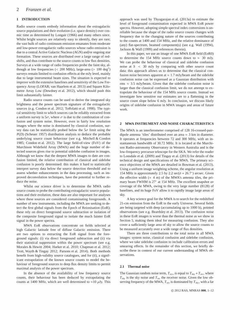
Figure 1. Top: central square degree of the MWA synthesised beam fora 2 min snapshot with a central frequency of 154 MHz and bandwidth of30.72 MHz, using a uniform weighting scheme. The peak is 1 Jy/beam andthe greyscale runs from –30 to 30 mJy/beam. The main lobe of the syn-thesised beam is saturated to clearly show the distant sidelobe structure.Bottom: standard deviation of the pixel values in the beam asa function ofdistance from the beam centre. This standard deviation was calculated in athin annulus at the given radius.

MWA synthesised beam for a 2 min snapshot with a central fre-quency of 154 MHz and bandwidth of 30.72 MHz, using a uniformweighting scheme. The standard deviation of the beam drops from≈ 1.3 × 10−2 at a distance of 10 arcmin from the beam centre to≈ 3.5× 10−4 at a distance of 13.5 deg from the beam centre (i.e. atthe half-power point), as shown in the bottom panel of Fig. 1.

3 MWA EOR DATA

Offringa et al. (2016) explored the effect of foreground spectra onEoR experiments by measuring spectra with high frequency reso-lution for the 586 brightest unresolved sources in the MWA EoR0field, centred at J2000α = 00h00m00s, δ = −27◦00′00′′. The ob-servations used in their work were spread over 12 nights between2013 August and 2013 October. They were made in two frequencybands covering 139− 170 MHz and 167− 198 MHz, with a fre-quency resolution of 40 kHz and time resolution of 0.5 s.

The mean rms noise over the central 10 degrees of theStokesI image integrated over the total 59 MHz bandwidth was3.6 mJy/beam after 5 h of integration. The rms noise continued todecline after 5 h of integration but not proportionally to 1/

√t: an

c© 2012 RAS, MNRAS000, 1–12

4 Franzen et al.

rms noise of 3.2 mJy/beam was reached after 45 h of integration.The rms noise in the StokesV image continued to follow 1/

√t,

reaching a level of 0.6 mJy/beam after 45 h of integration. TheStokesV image was void of sources, except for weak sources thatappeared because of instrumental leakage. The StokesV leakagewas typically 0.1− 1 per cent of the StokesI flux density.

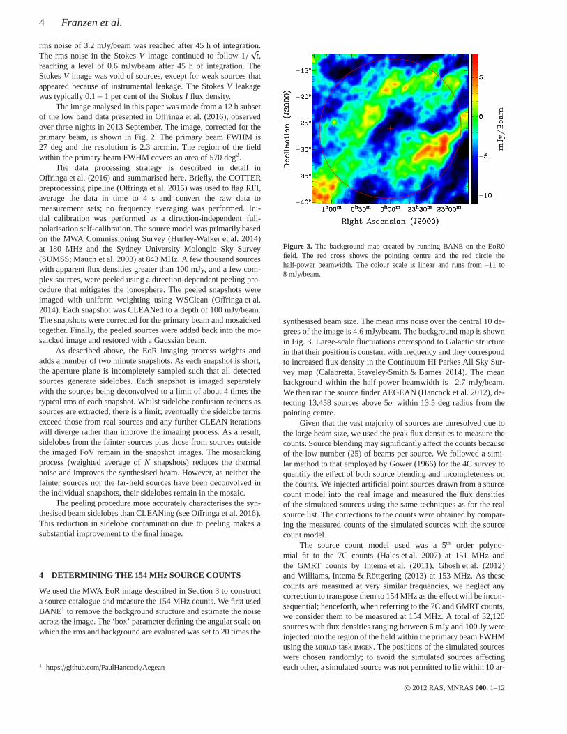
The image analysed in this paper was made from a 12 h subsetof the low band data presented in Offringa et al. (2016), observedover three nights in 2013 September. The image, corrected for theprimary beam, is shown in Fig. 2. The primary beam FWHM is27 deg and the resolution is 2.3 arcmin. The region of the fieldwithin the primary beam FWHM covers an area of 570 deg2.

The data processing strategy is described in detail inOffringa et al. (2016) and summarised here. Briefly, the COTTERpreprocessing pipeline (Offringa et al. 2015) was used to flag RFI,average the data in time to 4 s and convert the raw data tomeasurement sets; no frequency averaging was performed. Ini-tial calibration was performed as a direction-independentfull-polarisation self-calibration. The source model was primarily basedon the MWA Commissioning Survey (Hurley-Walker et al. 2014)at 180 MHz and the Sydney University Molonglo Sky Survey(SUMSS; Mauch et al. 2003) at 843 MHz. A few thousand sourceswith apparent flux densities greater than 100 mJy, and a few com-plex sources, were peeled using a direction-dependent peeling pro-cedure that mitigates the ionosphere. The peeled snapshotswereimaged with uniform weighting using WSClean (Offringa et al.2014). Each snapshot was CLEANed to a depth of 100 mJy/beam.The snapshots were corrected for the primary beam and mosaickedtogether. Finally, the peeled sources were added back into the mo-saicked image and restored with a Gaussian beam.

As described above, the EoR imaging process weights andadds a number of two minute snapshots. As each snapshot is short,the aperture plane is incompletely sampled such that all detectedsources generate sidelobes. Each snapshot is imaged separatelywith the sources being deconvolved to a limit of about 4 timesthetypical rms of each snapshot. Whilst sidelobe confusion reduces assources are extracted, there is a limit; eventually the sidelobe termsexceed those from real sources and any further CLEAN iterationswill diverge rather than improve the imaging process. As a result,sidelobes from the fainter sources plus those from sources outsidethe imaged FoV remain in the snapshot images. The mosaickingprocess (weighted average ofN snapshots) reduces the thermalnoise and improves the synthesised beam. However, as neither thefainter sources nor the far-field sources have been deconvolved inthe individual snapshots, their sidelobes remain in the mosaic.

The peeling procedure more accurately characterises the syn-thesised beam sidelobes than CLEANing (see Offringa et al. 2016).This reduction in sidelobe contamination due to peeling makes asubstantial improvement to the final image.

4 DETERMINING THE 154 MHz SOURCE COUNTS

We used the MWA EoR image described in Section 3 to constructa source catalogue and measure the 154 MHz counts. We first usedBANE1 to remove the background structure and estimate the noiseacross the image. The ‘box’ parameter defining the angular scale onwhich the rms and background are evaluated was set to 20 timesthe

1 https://github.com/PaulHancock/Aegean

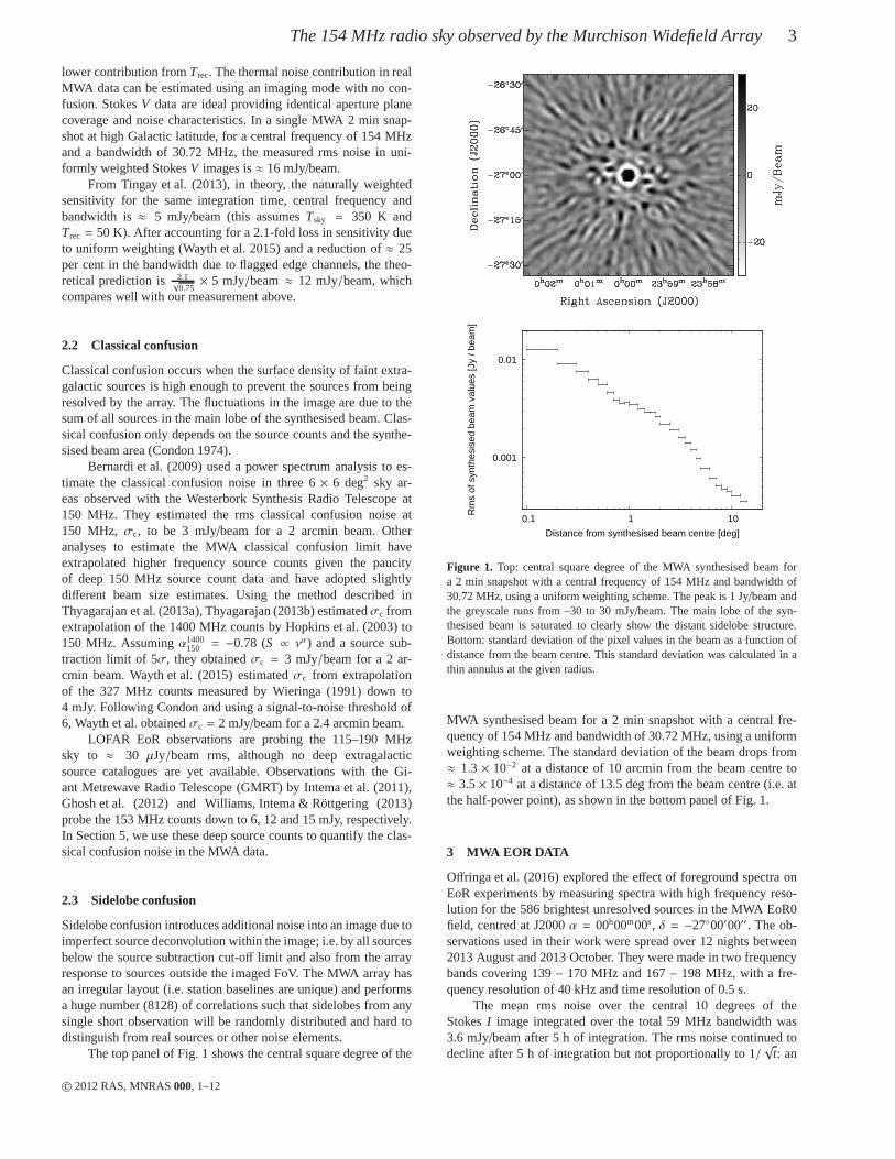
Figure 3. The background map created by running BANE on the EoR0field. The red cross shows the pointing centre and the red circle thehalf-power beamwidth. The colour scale is linear and runs from –11 to8 mJy/beam.

synthesised beam size. The mean rms noise over the central 10de-grees of the image is 4.6 mJy/beam. The background map is shownin Fig. 3. Large-scale fluctuations correspond to Galactic structurein that their position is constant with frequency and they correspondto increased flux density in the Continuum HI Parkes All Sky Sur-vey map (Calabretta, Staveley-Smith & Barnes 2014). The meanbackground within the half-power beamwidth is –2.7 mJy/beam.We then ran the source finder AEGEAN (Hancock et al. 2012), de-tecting 13,458 sources above 5σ within 13.5 deg radius from thepointing centre.

Given that the vast majority of sources are unresolved due tothe large beam size, we used the peak flux densities to measurethecounts. Source blending may significantly affect the counts becauseof the low number (25) of beams per source. We followed a simi-lar method to that employed by Gower (1966) for the 4C survey toquantify the effect of both source blending and incompleteness onthe counts. We injected artificial point sources drawn from asourcecount model into the real image and measured the flux densitiesof the simulated sources using the same techniques as for therealsource list. The corrections to the counts were obtained by compar-ing the measured counts of the simulated sources with the sourcecount model.

The source count model used was a 5th order polyno-mial fit to the 7C counts (Hales et al. 2007) at 151 MHz andthe GMRT counts by Intema et al. (2011), Ghosh et al. (2012)and Williams, Intema & Rottgering (2013) at 153 MHz. As thesecounts are measured at very similar frequencies, we neglectanycorrection to transpose them to 154 MHz as the effect will be incon-sequential; henceforth, when referring to the 7C and GMRT counts,we consider them to be measured at 154 MHz. A total of 32,120sources with flux densities ranging between 6 mJy and 100 Jy wereinjected into the region of the field within the primary beam FWHMusing themiriad taskimgen. The positions of the simulated sourceswere chosen randomly; to avoid the simulated sources affectingeach other, a simulated source was not permitted to lie within 10 ar-

c© 2012 RAS, MNRAS000, 1–12

The 154 MHz radio sky observed by the Murchison Widefield Array 5

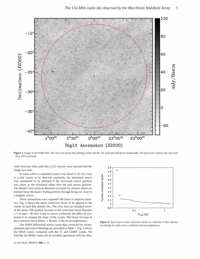
Figure 2. Image of the EoR0 field. The red cross shows the pointing centre and the red circle the half-power beamwidth. The greyscaleis linear and runs from–30 to 100 mJy/beam.

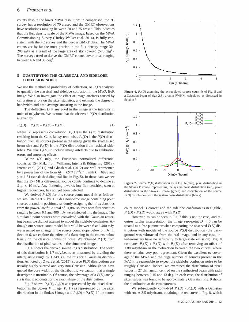
cmin from any other and only 3,212 sources were injected intotheimage at a time.

In cases where a simulated source was found to lie too closeto a real source to be detected separately, the simulated sourcewas considered to be detected if the recovered source positionwas closer to the simulated rather than the real source position.The Monte Carlo analysis therefore accounts for sources which areomitted from the source finding process through being too close toa brighter source.

These simulations were repeated 100 times to improve statis-tics. Fig. 4 shows the mean correction factor to be applied tothecounts in each flux density bin. The error bars are standard errorsof the mean. The gradual increase in the correction factor between≈ 1 Jy and≈ 40 mJy is due to source confusion; the effect of con-fusion is to steepen the slope of the counts. The sharp increase inthe correction factor below≈ 40 mJy is due to incompleteness.

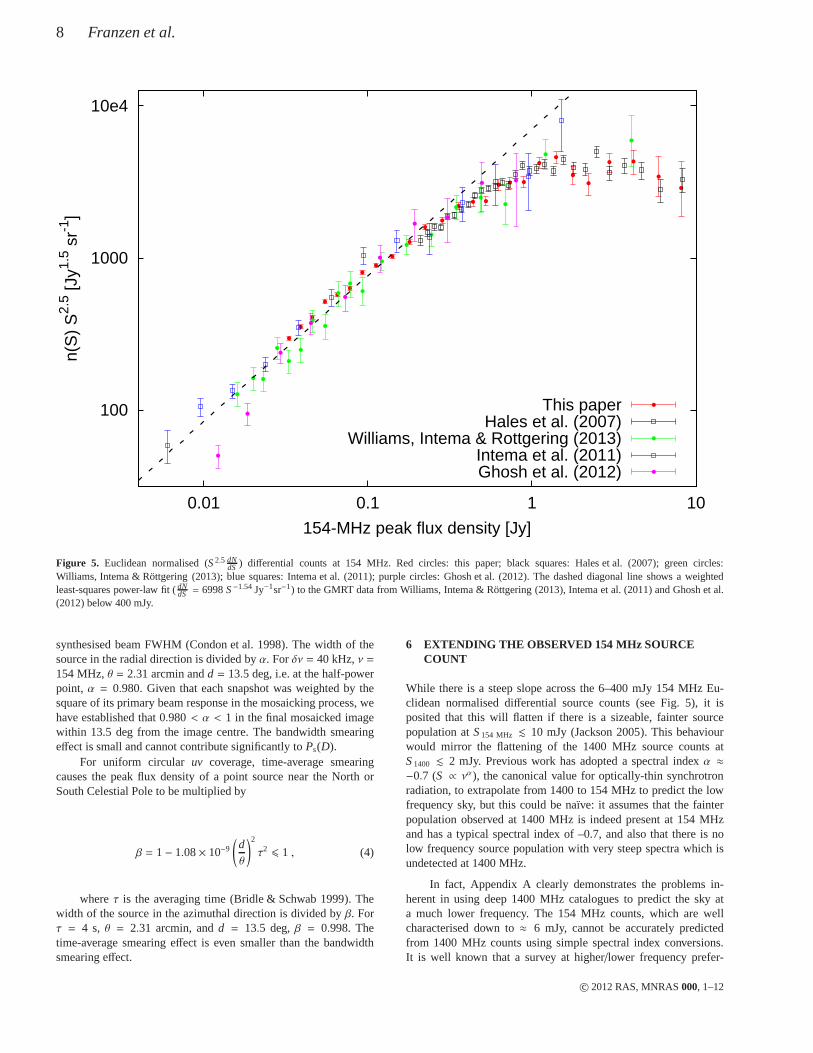
Our MWA differential source count data corrected for incom-pleteness and source blending are provided in Table 1. Fig. 5showsthe MWA counts compared with the 7C and GMRT counts. Wefind that the MWA counts are in excellent agreement with the other

0.9

1

1.1

1.2

1.3

1.4

1.5

1.6

1.7

1.8

1.9

0.1 1

Cou

nts

corr

ectio

n fa

ctor

S154 [Jy]

Figure 4. Top: Source count correction factor as a function of flux density,accounting for both source confusion and incompleteness.

c© 2012 RAS, MNRAS000, 1–12

6 Franzen et al.

counts despite the lower MWA resolution: in comparison, the7Csurvey has a resolution of 70 arcsec and the GMRT observationshave resolutions ranging between 20 and 25 arcsec. This indicatesthat the flux density scale of the MWA image, based on the MWACommissioning Survey (Hurley-Walker et al. 2014), is fullycon-sistent with the 7C survey and the deeper GMRT data. The MWAcounts are by far the most precise in the flux density range 30–200 mJy as a result of the large area of sky covered (570 deg2).The surveys used to derive the GMRT counts cover areas rangingbetween 6.6 and 30 deg2.

5 QUANTIFYING THE CLASSICAL AND SIDELOBECONFUSION NOISE

We use the method of probability of deflection, orP(D) analysis,to quantify the classical and sidelobe confusion in the MWA EoRimage. We also investigate the effect of image artefacts caused bycalibration errors on the pixel statistics, and estimate the degree ofbandwidth and time-average smearing in the image.

The deflectionD at any pixel in the image is the intensity inunits of mJy/beam. We assume that the observedP(D) distributionis given by

Po(D) = Pn(D) ∗ Pc(D) ∗ Ps(D), (1)

where ‘∗’ represents convolution,Pn(D) is the P(D) distributionresulting from the Gaussian system noise,Pc(D) is theP(D) distri-bution from all sources present in the image given the synthesisedbeam size andPs(D) is the P(D) distribution from residual side-lobes. We takePs(D) to include image artefacts due to calibrationerrors and smearing effects.

Below 400 mJy, the Euclidean normalised differentialcounts at 154 MHz from Williams, Intema & Rottgering (2013),Intema et al. (2011) and Ghosh et al. (2012) are well representedby a power law of the formdN

dS = kS−γ Jy−1sr−1, with k = 6998 andγ = 1.54 (see dashed diagonal line in Fig. 5). In these data we seethat the 154 MHz differential source counts continue to decline atS154 . 10 mJy. Any flattening towards low flux densities, seen athigher frequencies, has not yet been detected.

We derivedPc(D) for this source count model fit as follows:we simulated a 9.63 by 9.63 deg noise-free image containing pointsources at random positions, randomly assigning their flux densitiesfrom the power-law fit. A total of 51,887 sources with flux densitiesranging between 0.1 and 400 mJy were injected into the image.Thesimulated point sources were convolved with the Gaussian restor-ing beam; we did not attempt to model the sidelobe confusion.Al-though our source count model fit is valid between 6 and 400 mJy,we assumed no change in the source count slope below 6 mJy. InSection 6, we explore the effect of a flattening in the counts below6 mJy on the classical confusion noise. We obtainedPc(D) fromthe distribution of pixel values in the simulated image.

Fig. 6 shows the derived sourceP(D) distribution. The widthof this distribution is 1.7 mJy/beam, as measured by dividing theinterquartile range by 1.349, i.e. the rms for a Gaussian distribu-tion. As noted by Zwart et al. (2015), sourceP(D) distributions areusually highly skewed and very non-Gaussian. Although we havequoted the core width of the distribution, we caution that a singledescriptor is unsuitable. Of course, the advantage of aP(D) analy-sis is that it accounts for the exact shape of the distribution.

Fig. 7 showsPc(D), Pn(D) as represented by the pixel distri-bution in the StokesV image,Po(D) as represented by the pixeldistribution in the StokesI image andPc(D) ∗ Pn(D). If the source

0

0.2

0.4

0.6

0.8

1

1.2

0 1 2 3 4 5

PC

(D)

[(m

Jy /

beam

)-1]

D [mJy / beam]

Figure 6. Pc(D) assuming the extrapolated source count fit of Fig. 5 anda Gaussian beam of size 2.31 arcmin FWHM, calculated as discussed inSection 5.

0

0.2

0.4

0.6

0.8

1

1.2

-15 -10 -5 0 5 10 15

P(D

) [(

mJy

/ be

am)-1

]

D [mJy / beam]

Pc(D)Pn(D)Po(D)

Pc(D) * Pn(D)

Figure 7. SourceP(D) distribution as in Fig. 6 (blue), pixel distribution inthe StokesV image, representing the system noise distribution (red), pixeldistribution in the StokesI image (green) and convolution of the sourceP(D) distribution with the system noise distribution (black).

count model is correct and the sidelobe confusion is negligible,Pc(D) ∗ Pn(D) would agree withPo(D).

However, as can be seen in Fig. 7 this is not the case, and re-quires further interpretation: the image zero-pointD = 0 can betreated as a free parameter when comparing the observedP(D) dis-tribution with models of the sourceP(D) distribution (the back-ground was subtracted from the real image, and in any case, in-terferometers have no sensitivity to large-scale emission). Fig. 8comparesPc(D) ∗ Pn(D) with Po(D) after removing an offset of1.88 mJy/beam in the x-direction between the two curves, wherethere remains very poor agreement. Given the excellentuv cover-age of the MWA and the huge number of sources present in theFoV, it is reasonable to expect the sidelobe confusion noiseto beroughly Gaussian. Indeed, we examined the distribution of pixelvalues in 27 thin annuli centred on the synthesised beam withradiiranging between 0.15 and 13 deg. In each case, the distribution ofpixel values was found to be approximately Gaussian. Fig. 9 showsthe distribution at the two extremes.

We subsequently convolvedPc(D) ∗ Pn(D) with a Gaussianwith rms= 3.5 mJy/beam, obtaining the red curve in Fig. 8, which

c© 2012 RAS, MNRAS000, 1–12

The 154 MHz radio sky observed by the Murchison Widefield Array 7

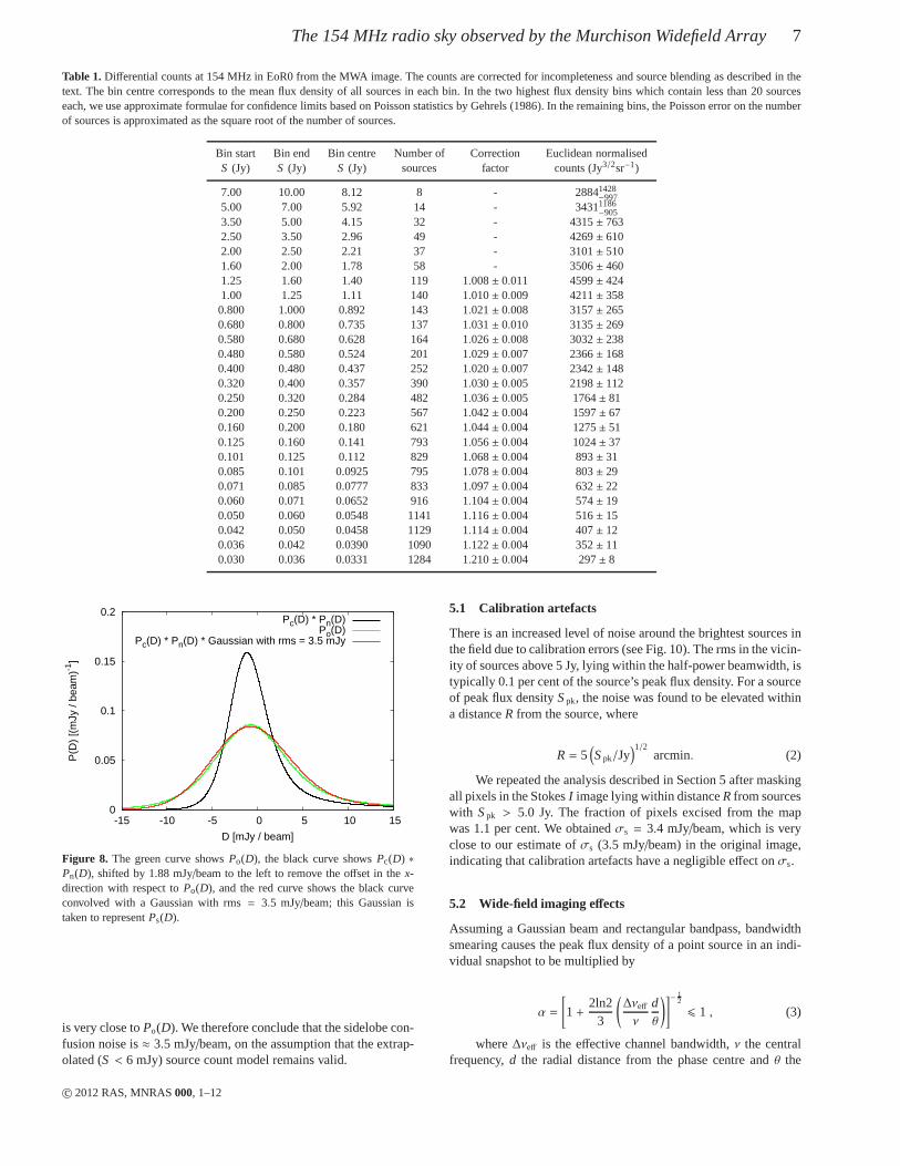
Table 1.Differential counts at 154 MHz in EoR0 from the MWA image. The counts are corrected for incompleteness and source blending as described in thetext. The bin centre corresponds to the mean flux density of all sources in each bin. In the two highest flux density bins which contain less than 20 sourceseach, we use approximate formulae for confidence limits based on Poisson statistics by Gehrels (1986). In the remaining bins, the Poisson error on the numberof sources is approximated as the square root of the number ofsources.

Bin start Bin end Bin centre Number of Correction Euclidean normalisedS (Jy) S (Jy) S (Jy) sources factor counts (Jy3/2sr−1)

7.00 10.00 8.12 8 - 28841428−997

5.00 7.00 5.92 14 - 34311186−905

3.50 5.00 4.15 32 - 4315± 7632.50 3.50 2.96 49 - 4269± 6102.00 2.50 2.21 37 - 3101± 5101.60 2.00 1.78 58 - 3506± 4601.25 1.60 1.40 119 1.008± 0.011 4599± 4241.00 1.25 1.11 140 1.010± 0.009 4211± 3580.800 1.000 0.892 143 1.021± 0.008 3157± 2650.680 0.800 0.735 137 1.031± 0.010 3135± 2690.580 0.680 0.628 164 1.026± 0.008 3032± 2380.480 0.580 0.524 201 1.029± 0.007 2366± 1680.400 0.480 0.437 252 1.020± 0.007 2342± 1480.320 0.400 0.357 390 1.030± 0.005 2198± 1120.250 0.320 0.284 482 1.036± 0.005 1764± 810.200 0.250 0.223 567 1.042± 0.004 1597± 670.160 0.200 0.180 621 1.044± 0.004 1275± 510.125 0.160 0.141 793 1.056± 0.004 1024± 370.101 0.125 0.112 829 1.068± 0.004 893± 310.085 0.101 0.0925 795 1.078± 0.004 803± 290.071 0.085 0.0777 833 1.097± 0.004 632± 220.060 0.071 0.0652 916 1.104± 0.004 574± 190.050 0.060 0.0548 1141 1.116± 0.004 516± 150.042 0.050 0.0458 1129 1.114± 0.004 407± 120.036 0.042 0.0390 1090 1.122± 0.004 352± 110.030 0.036 0.0331 1284 1.210± 0.004 297± 8

0

0.05

0.1

0.15

0.2

-15 -10 -5 0 5 10 15

P(D

) [(

mJy

/ be

am)-1

]

D [mJy / beam]

Pc(D) * Pn(D)Po(D)

Pc(D) * Pn(D) * Gaussian with rms = 3.5 mJy

Figure 8. The green curve showsPo(D), the black curve showsPc(D) ∗Pn(D), shifted by 1.88 mJy/beam to the left to remove the offset in thex-direction with respect toPo(D), and the red curve shows the black curveconvolved with a Gaussian with rms= 3.5 mJy/beam; this Gaussian istaken to representPs(D).

is very close toPo(D). We therefore conclude that the sidelobe con-fusion noise is≈ 3.5 mJy/beam, on the assumption that the extrap-olated (S < 6 mJy) source count model remains valid.

5.1 Calibration artefacts

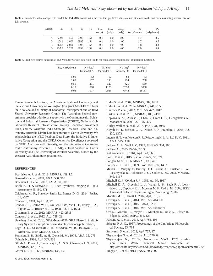
There is an increased level of noise around the brightest sources inthe field due to calibration errors (see Fig. 10). The rms in the vicin-ity of sources above 5 Jy, lying within the half-power beamwidth, istypically 0.1 per cent of the source’s peak flux density. For asourceof peak flux densitySpk, the noise was found to be elevated withina distanceR from the source, where

R= 5(

Spk/Jy)1/2

arcmin. (2)

We repeated the analysis described in Section 5 after maskingall pixels in the StokesI image lying within distanceRfrom sourceswith Spk > 5.0 Jy. The fraction of pixels excised from the mapwas 1.1 per cent. We obtainedσs = 3.4 mJy/beam, which is veryclose to our estimate ofσs (3.5 mJy/beam) in the original image,indicating that calibration artefacts have a negligible effect onσs.

5.2 Wide-field imaging effects

Assuming a Gaussian beam and rectangular bandpass, bandwidthsmearing causes the peak flux density of a point source in an indi-vidual snapshot to be multiplied by

α =

[

1+2ln2

3

(

∆νeff

ν

dθ

)]− 12

6 1 , (3)

where∆νeff is the effective channel bandwidth,ν the centralfrequency,d the radial distance from the phase centre andθ the

c© 2012 RAS, MNRAS000, 1–12

8 Franzen et al.

100

1000

10e4

0.01 0.1 1 10

n(S

) S

2.5 [J

y1.5 s

r-1]

154-MHz peak flux density [Jy]

This paperHales et al. (2007)

Williams, Intema & Rottgering (2013)Intema et al. (2011)Ghosh et al. (2012)

Figure 5. Euclidean normalised (S2.5 dNdS ) differential counts at 154 MHz. Red circles: this paper; black squares: Hales et al. (2007); green circles:

Williams, Intema & Rottgering (2013); blue squares: Intema et al. (2011); purple circles: Ghosh et al. (2012). The dashed diagonal line shows a weightedleast-squares power-law fit (dN

dS = 6998S−1.54 Jy−1sr−1) to the GMRT data from Williams, Intema & Rottgering (2013), Intema et al. (2011) and Ghosh et al.(2012) below 400 mJy.

synthesised beam FWHM (Condon et al. 1998). The width of thesource in the radial direction is divided byα. Forδν = 40 kHz,ν =154 MHz,θ = 2.31 arcmin andd = 13.5 deg, i.e. at the half-powerpoint, α = 0.980. Given that each snapshot was weighted by thesquare of its primary beam response in the mosaicking process, wehave established that 0.980 < α < 1 in the final mosaicked imagewithin 13.5 deg from the image centre. The bandwidth smearingeffect is small and cannot contribute significantly toPs(D).

For uniform circular uv coverage, time-average smearingcauses the peak flux density of a point source near the North orSouth Celestial Pole to be multiplied by

β = 1− 1.08× 10−9

(

dθ

)2

τ2 6 1 , (4)

whereτ is the averaging time (Bridle & Schwab 1999). Thewidth of the source in the azimuthal direction is divided byβ. Forτ = 4 s, θ = 2.31 arcmin, andd = 13.5 deg,β = 0.998. Thetime-average smearing effect is even smaller than the bandwidthsmearing effect.

6 EXTENDING THE OBSERVED 154 MHz SOURCECOUNT

While there is a steep slope across the 6–400 mJy 154 MHz Eu-clidean normalised differential source counts (see Fig. 5), it isposited that this will flatten if there is a sizeable, faintersourcepopulation atS154 MHz . 10 mJy (Jackson 2005). This behaviourwould mirror the flattening of the 1400 MHz source counts atS1400 . 2 mJy. Previous work has adopted a spectral indexα ≈−0.7 (S ∝ να), the canonical value for optically-thin synchrotronradiation, to extrapolate from 1400 to 154 MHz to predict thelowfrequency sky, but this could be naıve: it assumes that the fainterpopulation observed at 1400 MHz is indeed present at 154 MHzand has a typical spectral index of –0.7, and also that there is nolow frequency source population with very steep spectra which isundetected at 1400 MHz.

In fact, Appendix A clearly demonstrates the problems in-herent in using deep 1400 MHz catalogues to predict the sky ata much lower frequency. The 154 MHz counts, which are wellcharacterised down to≈ 6 mJy, cannot be accurately predictedfrom 1400 MHz counts using simple spectral index conversions.It is well known that a survey at higher/lower frequency prefer-

c© 2012 RAS, MNRAS000, 1–12

The 154 MHz radio sky observed by the Murchison Widefield Array 9

0

20

40

60

80

100

120

140

160

-0.03 -0.02 -0.01 0 0.01 0.02 0.03

Num

ber

of p

ixel

s

Synthesised beam value [Jy / beam]

0

20000

40000

60000

80000

100000

120000

140000

160000

180000

-0.001 -0.0005 0 0.0005 0.001

Num

ber

of p

ixel

s

Synthesised beam value [Jy / beam]

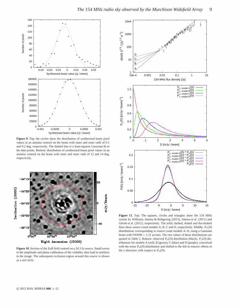
Figure 9. Top: the circles show the distribution of synthesised beam pixelvalues in an annulus centred on the beam with inner and outer radii of 0.1and 0.2 deg, respectively. The dashed line is a least-squares Gaussian fit tothe data points. Bottom: distribution of synthesised beam pixel values in anannulus centred on the beam with inner and outer radii of 12 and 14 deg,respectively.

Figure 10.Section of the EoR field centred on a 24.3 Jy source. Small errorsin the amplitude and phase calibration of the visibility data lead to artefactsin the image. The subsequent exclusion region around this source is shownas a red circle.

1

10

100

1000

10e4

10e-4 0.001 0.01 0.1 1 10

dN/d

S S

2.5 /

[Jy1.

5 sr-1

]

154-MHz flux density [Jy]

A

B

C

D

0

0.2

0.4

0.6

0.8

1

1.2

0 1 2 3 4 5 6

PC

(D)

[(m

Jy /

beam

)-1]

D [mJy / beam]

Pc, model A(D)Pc, model B(D)Pc, model C(D)Pc, model D(D)

0

0.05

0.1

0.15

0.2

-15 -10 -5 0 5 10 15

P(D

) [(

mJy

/ be

am)-1

]

D [mJy / beam]

Pc, model A(D) * Pn(D)Pc, model B(D) * Pn(D)Pc, model C(D) * Pn(D)Pc, model D(D) * Pn(D)

Po(D)

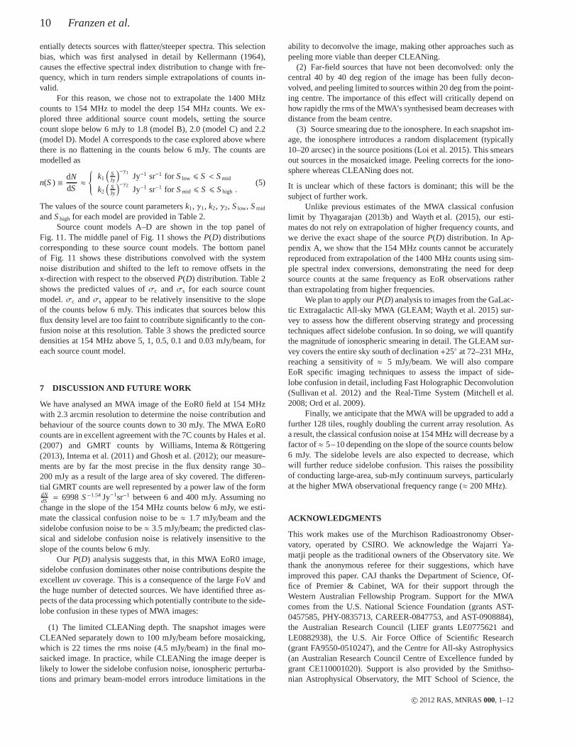
Figure 11. Top: The squares, circles and triangles show the 154 MHzcounts by Williams, Intema & Rottgering (2013), Intema et al. (2011) andGhosh et al. (2012), respectively. The solid, dashed, dotted and dot-dashedlines show source count models A, B, C and D, respectively. Middle:Pc(D)distributions corresponding to source count models A–D, using a Gaussianbeam with FWHM= 2.31 arcmin. The rms values of these distributions arequoted in Table 2. Bottom: observedPo(D) distribution (black),Pc(D) dis-tributions for models A (red), B (green), C (blue) and D (purple), convolvedwith the noisePn(D) distribution and shifted to the left to remove offsets inthe x-direction with respect toPo(D).

c© 2012 RAS, MNRAS000, 1–12

10 Franzen et al.

entially detects sources with flatter/steeper spectra. This selectionbias, which was first analysed in detail by Kellermann (1964),causes the effective spectral index distribution to change with fre-quency, which in turn renders simple extrapolations of counts in-valid.

For this reason, we chose not to extrapolate the 1400 MHzcounts to 154 MHz to model the deep 154 MHz counts. We ex-plored three additional source count models, setting the sourcecount slope below 6 mJy to 1.8 (model B), 2.0 (model C) and 2.2(model D). Model A corresponds to the case explored above wherethere is no flattening in the counts below 6 mJy. The counts aremodelled as

n(S) ≡dNdS≈

k1

(

SJy

)−γ1Jy−1 sr−1 for Slow 6 S < Smid

k2

(

SJy

)−γ2Jy−1 sr−1 for Smid 6 S 6 Shigh .

(5)

The values of the source count parametersk1, γ1, k2, γ2, Slow, Smid

andShigh for each model are provided in Table 2.Source count models A–D are shown in the top panel of

Fig. 11. The middle panel of Fig. 11 shows theP(D) distributionscorresponding to these source count models. The bottom panelof Fig. 11 shows these distributions convolved with the systemnoise distribution and shifted to the left to remove offsets in thex-direction with respect to the observedP(D) distribution. Table 2shows the predicted values ofσc and σs for each source countmodel.σc andσs appear to be relatively insensitive to the slopeof the counts below 6 mJy. This indicates that sources below thisflux density level are too faint to contribute significantly to the con-fusion noise at this resolution. Table 3 shows the predictedsourcedensities at 154 MHz above 5, 1, 0.5, 0.1 and 0.03 mJy/beam, foreach source count model.

7 DISCUSSION AND FUTURE WORK

We have analysed an MWA image of the EoR0 field at 154 MHzwith 2.3 arcmin resolution to determine the noise contribution andbehaviour of the source counts down to 30 mJy. The MWA EoR0counts are in excellent agreement with the 7C counts by Haleset al.(2007) and GMRT counts by Williams, Intema & Rottgering(2013), Intema et al. (2011) and Ghosh et al. (2012); our measure-ments are by far the most precise in the flux density range 30–200 mJy as a result of the large area of sky covered. The differen-tial GMRT counts are well represented by a power law of the formdNdS = 6998S−1.54 Jy−1sr−1 between 6 and 400 mJy. Assuming nochange in the slope of the 154 MHz counts below 6 mJy, we esti-mate the classical confusion noise to be≈ 1.7 mJy/beam and thesidelobe confusion noise to be≈ 3.5 mJy/beam; the predicted clas-sical and sidelobe confusion noise is relatively insensitive to theslope of the counts below 6 mJy.

Our P(D) analysis suggests that, in this MWA EoR0 image,sidelobe confusion dominates other noise contributions despite theexcellentuv coverage. This is a consequence of the large FoV andthe huge number of detected sources. We have identified threeas-pects of the data processing which potentially contribute to the side-lobe confusion in these types of MWA images:

(1) The limited CLEANing depth. The snapshot images wereCLEANed separately down to 100 mJy/beam before mosaicking,which is 22 times the rms noise (4.5 mJy/beam) in the final mo-saicked image. In practice, while CLEANing the image deeperislikely to lower the sidelobe confusion noise, ionospheric perturba-tions and primary beam-model errors introduce limitationsin the

ability to deconvolve the image, making other approaches such aspeeling more viable than deeper CLEANing.

(2) Far-field sources that have not been deconvolved: only thecentral 40 by 40 deg region of the image has been fully decon-volved, and peeling limited to sources within 20 deg from thepoint-ing centre. The importance of this effect will critically depend onhow rapidly the rms of the MWA’s synthesised beam decreases withdistance from the beam centre.

(3) Source smearing due to the ionosphere. In each snapshot im-age, the ionosphere introduces a random displacement (typically10–20 arcsec) in the source positions (Loi et al. 2015). Thissmearsout sources in the mosaicked image. Peeling corrects for theiono-sphere whereas CLEANing does not.

It is unclear which of these factors is dominant; this will bethesubject of further work.

Unlike previous estimates of the MWA classical confusionlimit by Thyagarajan (2013b) and Wayth et al. (2015), our esti-mates do not rely on extrapolation of higher frequency counts, andwe derive the exact shape of the sourceP(D) distribution. In Ap-pendix A, we show that the 154 MHz counts cannot be accuratelyreproduced from extrapolation of the 1400 MHz counts using sim-ple spectral index conversions, demonstrating the need fordeepsource counts at the same frequency as EoR observations ratherthan extrapolating from higher frequencies.

We plan to apply ourP(D) analysis to images from the GaLac-tic Extragalactic All-sky MWA (GLEAM; Wayth et al. 2015) sur-vey to assess how the different observing strategy and processingtechniques affect sidelobe confusion. In so doing, we will quantifythe magnitude of ionospheric smearing in detail. The GLEAM sur-vey covers the entire sky south of declination+25◦ at 72–231 MHz,reaching a sensitivity of≈ 5 mJy/beam. We will also compareEoR specific imaging techniques to assess the impact of side-lobe confusion in detail, including Fast Holographic Deconvolution(Sullivan et al. 2012) and the Real-Time System (Mitchell etal.2008; Ord et al. 2009).

Finally, we anticipate that the MWA will be upgraded to add afurther 128 tiles, roughly doubling the current array resolution. Asa result, the classical confusion noise at 154 MHz will decrease by afactor of≈ 5−10 depending on the slope of the source counts below6 mJy. The sidelobe levels are also expected to decrease, whichwill further reduce sidelobe confusion. This raises the possibilityof conducting large-area, sub-mJy continuum surveys, particularlyat the higher MWA observational frequency range (≈ 200 MHz).

ACKNOWLEDGMENTS

This work makes use of the Murchison Radioastronomy Obser-vatory, operated by CSIRO. We acknowledge the Wajarri Ya-matji people as the traditional owners of the Observatory site. Wethank the anonymous referee for their suggestions, which haveimproved this paper. CAJ thanks the Department of Science, Of-fice of Premier & Cabinet, WA for their support through theWestern Australian Fellowship Program. Support for the MWAcomes from the U.S. National Science Foundation (grants AST-0457585, PHY-0835713, CAREER-0847753, and AST-0908884),the Australian Research Council (LIEF grants LE0775621 andLE0882938), the U.S. Air Force Office of Scientific Research(grant FA9550-0510247), and the Centre for All-sky Astrophysics(an Australian Research Council Centre of Excellence funded bygrant CE110001020). Support is also provided by the Smithso-nian Astrophysical Observatory, the MIT School of Science,the

c© 2012 RAS, MNRAS000, 1–12

The 154 MHz radio sky observed by the Murchison Widefield Array 11

Table 2.Parameter values adopted to model the 154 MHz counts with theresultant predicted classical and sidelobe confusion noise assuming a beam size of2.31 arcmin.

Model k1 γ1 k2 γ2 Slow Smid Shigh σc σs

(mJy) (mJy) (mJy) (mJy/beam) (mJy/beam)

A 6998 1.54 6998 1.54 0.1 6.0 400 1.7 3.5B 1841 1.800 6998 1.54 0.1 6.0 400 1.7 3.5C 661.8 2.000 6998 1.54 0.1 6.0 400 1.8 3.4D 237.9 2.200 6998 1.54 0.1 6.0 400 2.0 3.4

Table 3.Predicted source densities at 154 MHz for various detectionlimits for each source count model explored in Section 6.

Slim /mJy/beam N/ deg2 N / deg2 N / deg2 N / deg2

for model A for model B for model C for model D

5.00 62 62 63 631.00 157 190 224 2680.50 231 320 425 5800.10 560 1125 2038 38380.03 1077 2925 6742 16187

Raman Research Institute, the Australian National University, andthe Victoria University of Wellington (via grant MED-E1799fromthe New Zealand Ministry of Economic Development and an IBMShared University Research Grant). The Australian Federalgov-ernment provides additional support via the Commonwealth Scien-tific and Industrial Research Organisation (CSIRO), National Col-laborative Research Infrastructure Strategy, Education InvestmentFund, and the Australia India Strategic Research Fund, and As-tronomy Australia Limited, under contract to Curtin University. Weacknowledge the iVEC Petabyte Data Store, the Initiative inInno-vative Computing and the CUDA Center for Excellence sponsoredby NVIDIA at Harvard University, and the International Centre forRadio Astronomy Research (ICRAR), a Joint Venture of CurtinUniversity and The University of Western Australia, fundedby theWestern Australian State government.

REFERENCES

Beardsley A. P. et al., 2013, MNRAS, 429, L5Bernardi G. et al., 2009, A&A, 500, 965Bowman J. D. et al., 2013, PASA, 30, e031Bridle A. H. & Schwab F. R., 1999, Synthesis Imaging in Radio

Astronomy II, 180, 371Calabretta M. R., Staveley-Smith L., Barnes D. G., 2014, PASA,

31, e007Condon J., 1974, ApJ, 188, 279Condon J. J., Cotton W. D., Greisen E. W., Yin Q. F., Perley R. A.,

Taylor G. B., Broderick J. J., 1998, AJ, 115, 1693Chapman E. et al., 2012, MNRAS, 423, 2518Condon J. J. et al., 2012, ApJ, 758, 23Dewdney P. et al., 2010, SKAMemo #130, SKA Phase 1: Prelimi-

nary System Description, www.skatelescope.org/publications/Edge D. O., Shakeshaft J. R., McAdam W. B., Baldwin J. E.,

Archer S., 1959, MNRAS, 68, 37Fomalont E. B., Bridle A. H., Davis M. M., 1974, A&A, 36, 273Gehrels N., 1986, ApJ, 303, 336Ghosh A., Prasad J., Bharadwaj S., Ali S. S., Chengalur J. N.,2012,

MNRAS, 426, 3295Gower J. F. R., 1966, MNRAS, 133, 151

Hales S. et al., 2007, MNRAS, 382, 1639Hales C. A. et al., 2014, MNRAS, 441, 2555Hancock P. et al., 2012, MNRAS, 422, 1812Harker G. et al., 2010, MNRAS, 405, 2492Hopkins A. M., Afonso J., Chan B., Cram L. E., Georgakakis A.,

Mobasher B., 2003, AJ, 125, 465Hurley-Walker N. et al., 2014, PASA, 31, e045Huynh M. T., Jackson C. A., Norris R. P., Prandoni I., 2005, AJ,

130, 1373Intema H. T., van Weeren R. J., Rottgering H. J. A., Lal D. V.,2011,

A&A, 535, A38Jackson C. A., Wall J. V., 1999, MNRAS, 304, 160Jackson C., 2005, PASA, 22, 36Kellermann K. I., 1964, ApJ, 140, 969Loi S. T. et al., 2015, Radio Science, 50, 574Longair M. S., 1966, MNRAS, 133, 421Lonsdale C. J. et al., 2009, Proc. IEEE, 97, 1497Mauch T., Murphy T., Buttery H. J., Curran J., Hunstead R. W.,

Piestrzynski B., Robertson J. G., Sadler E. M., 2003, MNRAS,342, 1117

Mitchell K. J., Condon J. J., 1985, AJ, 90, 1957Mitchell D. A., Greenhill L. J., Wayth R. B., Sault R. J., Lons-

dale C. J., Cappallo R. J., Morales M. F., Ord S. M., 2008, IEEEJournal of Selected Topics in Signal Processing, 2, 707

Morales M. F., Hewitt J., 2004, ApJ, 615, 7Offringa A. R. et al., 2014, MNRAS, 444, 606Offringa A. R. et al., 2015, PASA, 32, 8Offringa A. R. et al., 2016, MNRAS, submittedOrd S., Greenhill L., Wayth R., Mitchell D., Dale K., Pfister H.,

Edgar R., 2009, ASPC, 411, 127Parsons A. R. et al., 2014, ApJ, 788, 106Scheuer P. A. G., 1957, Proceedings of the Cambridge Philosophi-

cal Society, 53, 764Sullivan I. S. et al., 2012, ApJ, 759, 17Thyagarajan N. et al., 2013a, ApJ, 776, 6Thyagarajan N., 2013b, Notes on MWA 128T confu-

sion limits, MWA Technical Memo. Available at:http://mwa-lfd.haystack.mit.edu/knowledgetree/view.php?fDocumentId=826

Tingay S. J. et al., 2013, PASA, 30, e007

c© 2012 RAS, MNRAS000, 1–12

12 Franzen et al.

Toffolatti L., Argueso Gomez F., de Zotti G., Mazzei P., Frances-chini A., Danese L., Burigana C., 1998, MNRAS, 297, 117

Trott C. M., Wayth R. B., Tingay S. J., 2012, ApJ, 757, 101van Haarlem M. P. et al., 2013, A&A, 556, A2Wall J. V., 1994, AuJPh, 47, 625Wayth R. B. et al., 2015, PASA, 32, e025White R. L., Becker R. H., Helfand D. J., Gregg M. D., 1997, ApJ,

475, 479Wieringa M., 1991, PhD thesis, Leiden UniversityWilliams W. L., Intema H. T., Rottgering H. J. A., 2013, A&A,549,

A55Zwart J. et al., 2015, in Bourke T. L. et al., eds, Proc. Ad-

vancing Astrophysics with the Square Kilometre Array,Astronomy below the Survey Threshold, id. 172. Available at:http://pos.sissa.it/cgi-bin/reader/conf.cgi?confid=215#session-2110

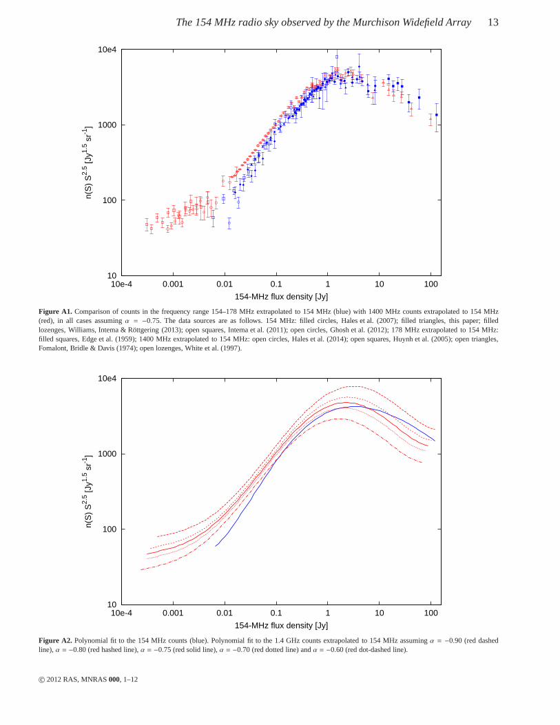
APPENDIX A: EXTRAPOLATING THE 1400 MHzCOUNTS TO PREDICT THE 154 MHz SKY

Fig. A1 shows counts in the frequency range 154–178 MHz extrap-olated to 154 MHz compared with 1400 MHz counts extrapolatedto 154 MHz, in all cases assuming a spectral index of –0.75. Itcanbe seen that extrapolation of the 1400 MHz counts to 154 MHz sig-nificantly overpredicts the 154 MHz counts below about 500 mJy.The density of sources atS154 = 6 mJy is overpredicted by about afactor of two.

Moreover, Fig. A2 shows that the 154 MHz counts above6 mJy cannot be accurately reproduced from extrapolation ofthe1.4 GHz counts usinganyspectral index; the best fit is obtained fora spectral index of –0.75. A polynomial fit to the 154 MHz countsis compared with a polynomial fit to the 1400 MHz counts extrapo-lated to 154 MHz assuming a spectral index of –0.90, –0.80, –0.75,–0.70 and –0.60. The integral of the squared difference between thetwo curves fromS154 = 6 mJy toS154 = 100 Jy is minimised forα = −0.75.

c© 2012 RAS, MNRAS000, 1–12

The 154 MHz radio sky observed by the Murchison Widefield Array 13

10

100

1000

10e4

10e-4 0.001 0.01 0.1 1 10 100

n(S

) S

2.5 [J

y1.5 s

r-1]

154-MHz flux density [Jy]

Figure A1. Comparison of counts in the frequency range 154–178 MHz extrapolated to 154 MHz (blue) with 1400 MHz counts extrapolatedto 154 MHz(red), in all cases assumingα = −0.75. The data sources are as follows. 154 MHz: filled circles, Hales et al. (2007); filled triangles, this paper; filledlozenges, Williams, Intema & Rottgering (2013); open squares, Intema et al. (2011); open circles, Ghosh et al. (2012);178 MHz extrapolated to 154 MHz:filled squares, Edge et al. (1959); 1400 MHz extrapolated to 154 MHz: open circles, Hales et al. (2014); open squares, Huynh et al. (2005); open triangles,Fomalont, Bridle & Davis (1974); open lozenges, White et al.(1997).

10

100

1000

10e4

10e-4 0.001 0.01 0.1 1 10 100

n(S

) S

2.5 [J

y1.5 s

r-1]

154-MHz flux density [Jy]

Figure A2. Polynomial fit to the 154 MHz counts (blue). Polynomial fit to the 1.4 GHz counts extrapolated to 154 MHz assumingα = −0.90 (red dashedline), α = −0.80 (red hashed line),α = −0.75 (red solid line),α = −0.70 (red dotted line) andα = −0.60 (red dot-dashed line).

c© 2012 RAS, MNRAS000, 1–12