the 3d electrical structure of the australian lithosphere · 2017-06-28 · 3d imaging of the...

The 3D Electrical Structure of the

Australian Lithosphere

Thesis submitted in accordance with the requirements of the University of Adelaide for an Honours Degree in Geophysics

Andrew Jon May

November 2013

3D IMAGING OF THE AUSTRALIAN LITHOSPHERE 1

THE 3D ELECTRICAL STRUCTURE OF THE AUSTRALIAN LITHOSPHERE

ABSTRACT

The broad-scale electrical resistivity structure of the Australian continent is poorly

known due to the lack of continent-wide observations. These observations are used to

constrain lithospheric conduction and petrophysical conditions. In this study, models of

electrical resistivity are developed using various constraints, and these are tested against

known observations. Three approaches have been employed. Firstly, using the AWAGS

array of 58 magnetotelluric sites across Australia spaced approximately 500 km apart, I

analyse geomagnetic depth sounding induction vector data, which are then compared

with the broad-scale tectonic components of Australia. Secondly, I have developed an

upper crustal and surrounding ocean model of electrical conductance using ocean depth

information (ETOPO1) and depth to Proterozoic basement (SEEBASE) with a spatial

resolution of approximately 17 km. Thirdly, estimates of seismic shear wave velocity of

the lithosphere from 50 to 200 km depth from the AuSREM data, at a spatial resolution

of approximately 50 km, were converted to electrical resistivity using an empirical

relationship. The induction vectors were then compared with three dimensional

modelling developed through two approaches. To good approximation I have been able

to demonstrate, that the observed AWAGS induction vector data are explained to first

order by the conduction of the oceans and sedimentary basins. Second-order effects of

resistivity variations in the deeper lithosphere are significant, but induction vectors are

less sensitive to these. Finally, I demonstrate from a 3D inversion of the observed

AWAGS data that there are additional crustal conductors that cannot be explained from

sediment thickness alone, but require additional conduction mechanisms in the crust

over significant depths.

KEYWORDS

Electrical resistivity, conductance, lithosphere, Australia


Table of Contents The 3D Electrical Structure of the Australian Lithosphere ............................................. 1

Abstract ........................................................................................................................ 1 Keywords...................................................................................................................... 1

List of Figures and Tables ............................................................................................. 3 Introduction .................................................................................................................. 4 Background................................................................................................................... 6

Theory .......................................................................................................................... 9 Observed Data ............................................................................................................ 11

Methods .................................................................................................................. 11

Results .................................................................................................................... 14

Building an Australian Lithosphere Resistivity Model................................................. 17 Surface Conductance: Methods................................................................................ 17

Results .................................................................................................................... 18

Mantle Lithosphere Resistivity: Methods ................................................................. 19

Results .................................................................................................................... 22

Testing Observational Data ......................................................................................... 22 Thin Sheet Model: Methods..................................................................................... 22

Results .................................................................................................................... 23

3D Forward Model: Methods ................................................................................... 25

Results .................................................................................................................... 27

Testing Data................................................................................................................ 29 Thin-Sheet Inversion: Methods ................................................................................ 29

Results .................................................................................................................... 30

Discussion .................................................................................................................. 31 Observational Data .................................................................................................. 31

Modelled Data ......................................................................................................... 31

Comparison of Observational and Modelled Data .................................................... 32

Conclusion .................................................................................................................. 33

Acknowledgments ...................................................................................................... 34 References .................................................................................................................. 34


LIST OF FIGURES AND TABLES

Figure 1 Real (or in-phase) induction vectors plotted on top of Australia’s major

cratons and basins using the Parkinson convention at periods of 1000 s and 10 000 s.

The Charters Tower station, highlighted in the red square, is a region of notable change

in the periods (adapted from Betts et al. 2002). 16

Figure 2 Surface conductance derived from depth to basement topography and water

depth databases of the Australian continent with AWAGS induction vectors plotted at a

period of 1000 s. Areas of notably high conductance have been highlighted with red

circles, in particular the Canning Basin and the Arunta region. 18

Figure 3 The fit to the cross plot of 1/log (resistivity) against shear wave velocity at

five different cluster points represented by different colours. Each cluster point is fitted

with a robust centroid represented by the black dots as well as error bars one standard

deviation. Dashed black lines are inferences taken from a cross plot showing varying

water content in major lithospheric minerals such as olivine. The blue lines represent

expected extreme conditions such for water contents of 200, 300, and 0 in ppm for Opx,

Cpx and Gt respectively. Adapted from Jones et al. (2013). 20

Figure 4 Map view of resistivities at depths of 50 km and 100 km with a spatial

resolution of approximately 50 km, derived from the AuSREM shear-wave velocity and

the empirical relationship equation from Jones et al. (2013). Location of cratons and

basins are adapted from Betts et al. (2002) 21

Figure 5 Apparent resistivity plotted at 1000 s with the electrical field in a north-south

orientation (x) and the magnetic field in the east west orientation (y). Phase has been

plotted in the same orientation for the Australian continent. Major sedimentary basins

and the oceans surrounding Australia have a major effect on the MT responses, with

known sedimentary basins clearly identifiable within the MT responses. 24

Figure 6 Parameters set for the 3D forward model and the raw data sets. Adapted from

Wang and Lilley (1999). 25

Figure 7 The 3D forward model of the Australian continent represented in map view

from 0 to 5 km, 35 to 60 km, 60 to 85 km, and 85 to 110 km. Below is the observed

induction vector data at a period of 1000 s for comparison. 26

Figure 8 A) The forward model synthetic induction vectors plotted at 1000 s B)

AWAGS induction vectors plotted at a period of 1000 s for comparison. 28

Figure 9 Thin-sheet Inversion of real or in-phase induction vectors at a period of 1000

s. The inversion reveals five regions of anomalous conductance structures which up to

five times the conductance values as the continental background. These regions have

been highlighted with black circles. 30

Table 1 GDS sites including station number, code, latitude, longitude and elevation .. 12


INTRODUCTION

The Australian continent has experienced a long and complex tectonic history (Betts et

al. 2002). Imaging the internal structure and mapping of the lithosphere allows us to

better understand existing uncertainties such as the physical state of the crust and upper

mantle, the hydration state, lithospheric formation and deformation history (Jones 1999,

Jones et al. 2012, Selway 2013). The use of magnetotellurics (MT) and geomagnetic

depth sounding (GDS) allows us to image the electrical conductivity on a continental

scale (e.g. Evans et al. 2011, Jones et al. 2005, Bedrosian and Feucht 2013) providing

important constraints on the physical, chemical and thermal structure of the Australian

lithosphere.

Lithospheric properties are observed through various laboratory studies (Wang et al.

2006, Yoshino et al. 2006, Yoshino et al. 2009, e.g. Jones et al. 2012), as well as

petrological analysis of mantle xenoliths and seismic data (Jones et al. 2009). Other

deep geophysical studies include Kennett et al. (2011)the study of the Australian

lithosphere using seismic data sets to map the depth of the Australian Moho by Kennett

et al. (2011) and a study of the Australian mantle conducted by Fishwick and Rawlinson

(2012).

Recent regional scale MT work conducted in Australia includes studies conducted

beneath the Olympic Dam iron oxide copper-gold deposit by Heinson et al. (2006), and

a study conducted by Thiel and Heinson (2013) across the Gawler Craton in order to

provide constraints on tectonothermal events dating from the Proterozoic.


At the continental scale, major MT studies include the South African Magnetotelluric

Experiment (SAMTEX) (e.g. Evans et al. 2011), a study which involved over 700

stations in the Kaapvaal craton, a region in Southern Africa. Through the SAMTEX

experiment the authors have shown that the lithospheric mantle contains complex

structures with large variations in maximum resistivity at depths of 200-250 km. The

study was able to determine that beneath the Bushveld complex, the mantle is highly

conductive. Potential causes of this highly conductive region include graphite, sulphide

and/or iron metals which were associated with the Bushveld magmatic event (Evans et

al. 2011).

Continental scale studies have been conducted in Northern America using data from the

USArray project, a component of the EarthScope program in which a series of both

permanent and portable MT stations have been placed throughout the United States,

covering over 35 % of the continent (Bedrosian and Feucht 2013). Through this project,

numerous studies have been conducted (e.g. Evans et al. 2011, Zhdanov et al. 2011,

Kelbert et al. 2012, Shen et al. 2013). Most recently, the work of Bedrosian and Feucht

(2013), has provided a comprehensive overview of the structure and tectonics of the

north-western United States. Modelling by Bedrosian and Feucht (2013) was able to

provide constraints on the distribution of fluids and melt within the lithosphere, and it

produced a three-dimensional resistivity model that provides insights into the tectonic

assembly of Western North America from the Archean to the present.

.


In this study, I aim to use GDS induction data (e.g. Chamalaun and Barton 1990,

Chamalaun and Barton 1993, Milligan et al. 1993, Welsh et al. 1996), as well as

lithospheric-scale shear wave velocity, depth to crystalline basement, and water depth

databases to assess what can be learnt about the physical, chemical and thermal

structure of the Australian lithosphere.

BACKGROUND

The Australian continent itself can be broadly split into three zones, the Archean Shield

in the west, Proterozoic cratons in central Australia and the Phanerozoic fold belts in the

East. Lithospheric growth occurred via vertical and horizontal accretion (Betts et al.

2002), in three major episodes, each comprising approximately one third of the

continental area (Kennett et al. 2011). The Proterozoic was a major period of crustal

growth in which components of the North Australia, West Australian and South

Australian cratons were formed and amalgamated (Betts et al. 2002). The internal

structure of the continental lithosphere provides vital insights into its creation and

development (Jones 1999). Imaging of the internal structure is analysed through the use

of seismic and electromagnetic methods. Knowledge of the internal structure as well as

the geometry of the lithosphere-asthenosphere boundary is critically important for

developing our understanding of the dynamics of the Earth (Jones 1999, Selway 2013).

The lithosphere is defined as a strong layer at the surface and includes both the crust and

shallow upper mantle (Karato 2010). It forms a rigid mechanical boundary and is

underlain by a weak layer, the asthenosphere, which is characterised by plastic

deformation over large time periods (Eaton et al. 2009). The chemistry of the mantle is

dominated by olivine (Pommier 2013). Other major phases found in the lithosphere


include pyroxene and garnet, average trends of mantle composition suggest that the

mantle becomes increasingly depleted in incompatible elements (such as Fe, Al , Ca,

and radioactive elements) with increasing age (Poudjom Djomani et al. 2001).

The crust forms an integral piece of the lithosphere, and its thickness also plays a major

role in controlling the overall behaviour of the lithospheric formation to deformation

(Kennett and Salmon 2012).Thin and thick crust provide major contrasting differences

in that thin crust allows deformation to be localised in the mantle, whereas thick crust

allows stress accumulation within the crust (Kennett and Salmon 2012).

The lithosphere is non-convecting and as such is characterised by conductive

geotherms, although in some cases local magmatic activity has the potential to produce

a temporary advective geotherm (Y. O'Relly and Griffin 1985). The lithosphere-

asthenosphere boundary (LAB) represents the base of the Earth’s lithosphere and is

governed by a conductive thermal regime, which is isolated from the convecting

asthenosphere (O'Reilly and Griffin 2010). The LAB is a moveable boundary, becoming

shallower due to thermal and chemical erosion of the lithosphere and deeper through

processes such as subcretion of upwelling hot mantle plumes (O'Reilly and Griffin

2010).

Constraining the hydration state of the upper mantle is critical for understanding the

dynamics and geochemical evolution of the Australian continent (Yoshino et al. 2009).

The presence of water in nominally anhydrous minerals (NAM) has an effect on a

number of physical and chemical properties of mantle minerals, in particularly

enhancing electrical conductivity (Peslier et al. 2010). Hydrogen can be incorporated


into olivine, a major mineral phase in the mantle, and as such creates a hydrous olivine

which has a much higher conductivity when compared with anhydrous olivine (Yoshino

et al. 2006).

The rheological properties of Earth’s mantle control a number of important geological

processes within the upper mantle such as the style of mantle convection and the nature

of thermal evolution (Karato 2010). Direct estimations of rheological properties are

sourced from deformation experiments on rocks conducted in laboratories under

realistic/in-Earth pressure and temperatures (Karato and Wu 1993, Karato 2010).

Lithospheric properties are determined through various laboratory studies (e.g. Yoshino

et al. 2006, Yoshino et al. 2009, Jones et al. 2012), as well as petrological analysis of

mantle xenoliths and seismic data (Jones et al. 2009). The use of deep geophysical

studies provides another insight into the complex nature of the lithosphere which

laboratory studies cannot necessarily provide.

Many of the above mentioned lithospheric properties have an effect on the

electromagnetic responses recorded with MT. There are a number of critical factors

which affect electrical resistivity of the lithospheric mantle. Of these factors, resistivity

is governed, to the first order, by temperature variation, with a number of other

variables including chemistry, rheology and the hydration state (Fullea et al. 2011).


THEORY

The MT method is a passive geophysical technique, which is used to image the

electrical resistivity structure of the Earth’s crust and its upper mantle through the

measurement of time varying natural magnetic fields and the induced electric fields

(Simpson and Bahr 2005, Chave and Jones 2012). The MT theory is well established

and has been in routine use since 1969 (Chave and Jones 2012). Detailed MT theory,

discussions and fundamental equations can be found in reviews and text books, for

example Vozoff (1990), Simpson and Bahr (2005) and Chave and Jones (2012).

MT is a natural source electromagnetic (EM) method within the bandwidth of 0.001 s to

10,000 s. Through the penetration of EM waves into the Earth’s crust, currents are

induced in electrically conductive bodies. These currents then produce secondary

magnetic fields and through isolating these, the resistivity distribution associated with

the bodies of current can be mapped. The penetration depth is controlled by the skin-

depth (Simpson and Bahr 2005), δ (metres), of the sounding, according to the equation

𝛿 = 2/𝜇0𝜔𝜍

(1)

where 𝜔 is the angular frequency in radians of the external field, 𝜇0 is the free air

permeability (4𝜋 . 10−7 𝐻𝑚−1), and 𝜍 is the conductivity of the medium in Siemens

per metre. This equation can then be simplified to

𝛿 ≈ 500 𝜌𝑇

(2)


where 𝜌 is the resistivity in Ohm metres (Ω.m) and T is the period (Arora et al. 1999).

Induction vectors are derived from transfer functions that relate the vertical magnetic

field to the horizontal magnetic field, represented by the following equation:

where 𝑇𝑧𝑥 and 𝑇𝑧𝑦 are the complex valued transfer functions and 𝐵𝑥 , 𝐵𝑦 and 𝐵𝑧 form the

three components of the geomagnetic field.

Lateral resistivity changes can be shown by the use of the GDS induction vectors,

sometimes known as Parkinson induction arrows (Simpson and Bahr 2005). When

considering laterally uniform resistivity, there is no anomalous vertical magnetic field.

Induction vectors are sensitive to lateral conductivity differences, however are

comparatively insensitive to changes in resistivity with depth (Chave and Jones 2012).

Induction arrows are complex vectors which must have magnitude and direction as well

as real and imaginary components. The orientation of induction vectors can be given in

one of two conventions, Parkinson and Wiese conventions (Simpson and Bahr 2005). In

this paper I have adopted the Parkinson convention in which induction arrows point

towards more conductive regions.

𝐵𝑧 = 𝑇𝑧𝑥𝐵𝑥 + 𝑇𝑧𝑦𝐵𝑦

(3)


In the Parkinson’s convention there are two components to the induction vector (M), the

real (Re) and the imaginary (Im) component of T. Each component has amplitude:

𝑀𝑅𝑒= 𝑅𝑒(𝑇𝑥)2 + 𝑅(𝑇𝑦)2 and 𝑀𝐼𝑚 = 𝐼𝑚(𝑇𝑥)2 + 𝑖(𝑇𝑦)2

(4)

Directions of the real and imaginary arrows (positive clockwise from the geographic

north) are given by:

𝜃𝑅𝑒 = arctan

𝑅𝑒(𝑇𝑦)

𝑅𝑒(𝑇𝑥)

𝜃𝐼𝑚 = arctan𝐼𝑚(𝑇𝑦)

𝐼𝑚(𝑇𝑥)

(5)

R and i denote the real and imaginary parts of the transfer functions.

The trends of the induction vectors across different periods allow regional variations of

conductivity to be detected. Real arrows (or vectors) will point directly towards regions

of high conductivity.

OBSERVED DATA

Methods

Legacy GDS data have been compiled from various sources, including the Australia

Wide Array of Geomagnetic Stations (AWAGS) survey, which comprised 58 GDS

stations covering mainland Australia (Chamalaun and Barton 1990, Chamalaun and

Barton 1993, Welsh et al. 1996). Of the 58 stations, 54 were portable three-component


magnetometers and four were permanent magnetic observations (Chamalaun and

Walker, 1982). The geomagnetic field fluctuations were recorded at 1-minute intervals

with 1 nT sensitivity combined with sensor temperature and time. Data recording

commenced on the 18th of November 1989 and finished on the 17

th of December 1990

(Welsh et al. 1996). Other GDS data has been sourced from studies conducted in

Ballarat and Halls Creek (Milligan et al. 1993, Roberts et al. 2008). Details of the

respective stations are given in Table 1.

Table 1 GDS sites including station number, code, latitude, longitude and elevation

Station Station Code Latitude Longitude Elevation (m)

Data: AWAGS (Welsh et al. 1993)

47 ABY -34.945 117.805 75

21 ALP -23.655 146.587 420

18 ASP -23.807 133.898 540

49 BAL -34.624 143.573 64

26 BIR -25.91 139.352 55

36 BUK -30.052 145.952 117

45 CDN -33.063 147.213 217

42 CED -32.13 133.713 20

8 CKT -15.477 145.187 6

54 CNB -35.317 149.367 859

23 CNE -25.803 122.945 452

7 CRO -18.215 142.253 120

55 CTA -20.083 146.25 370

33 CVN -24.882 113.665 5

1 DAR -12.403 130.859 31

9 DER -17.37 123.663 5

5 DYW -16.273 133.373 230

32 EMU -28.63 132.198 300

48 ESP -33.685 121.822 150

34 ETA -28.718 138.633 300

41 EUC -31.682 128.88 5

13 GER -28.797 114.703 35

38 GFN -29.767 153.02 27

24 GIL -25.035 128.3 609

19 GLE -2.883 138.817 158

57 GNA -31.783 115.95 60

2 GOV -12.377 136.74 50

15 GRN -20.56 130.355 380

10 HAL -18.233 127.667 440


14 HED -20.377 118.63 4

12 ISA -20.667 139.49 341

17 KIW -22.867 127.55 450

30 LAV -28.612 122.422 462

56 LRM -22.217 114.1 4

58 MAC -16.273 133.373 230

29 MEK -26.61 118.545 518

44 MEN -32.4 142.417 61

37 MOR -29.498 149.847 230

25 MTD -26.067 135.245 62

51 MYB -25.523 152.728 10

46 NEW -32.796 151.836 7

50 POL -38.313 141.467 93

43 PTA -32.483 137.75 5

27 QUI -26.608 144.253 215

6 ROB -16.717 136.95 80

28 ROM -26.55 148.775 308

39 SOX -31.239 119.355 345

11 TCK -19.627 134.183 376

16 TEL -21.705 122.228 293

35 TIB -29.448 142.053 120

53 TOO -37.533 145.467 457

52 TWO -35.032 138.578 163

22 VER -24.23 118.237 400

31 WAN -28.51 129 310

1 WEI -12.68 141.925 19

20 WTN -22.367 143.082 215

4 WYN -15.51 128.147 5

40 ZAN -31.037 123.568 274

Data: Halls Creek (Roberts et al. 2008)

31 EMG -15.918 128.049 101

33 DUN -16.013 128.429 78

39 ORD -16.028 128.8 84

49 POP -16.677 128.26 252

48 SPC -16.719 128.92 175

34 NEG -17.354 129 198

42 PUR -17.411 128.202 301

54 PAN -17.878 127.832 333

29 NIC -18.033 128.993 386

22 FLO -18.314 128.563 372

43 KOO -18.455 127.581 467

47 LAM -18.553 127.236 354

15 MAR -18.635 126.968 320

16 RUB -18.763 127.721 404

46 WOL -19.088 127.672 363

Data: Ballarat (Milligan et al.1993)

3 BAL -37.583 143.743 455


11 BAL -37.699 143.599 352

19 BAL -37.725 143.736 459

99 BAL -37.515 143.789 439

5 BAL -37.597 143.580 388

14 BAL -37.849 143.605 215

26 BAL -37.726 143.911 389

37 BAL -37.523 143.905 581

52 BAL -37.011 143.015 218

The AWAGS, Ballarat and Halls Creek data were processed to industry standard

Electrical Data Interchange (EDI) format using a robust bounded influence remote

referencing method BIRRP; Bounded Influence, Remote Reference Processing (Chave

and Thomson 2004). The EDI files were imported into WinGlink in order to create a

map of regional GDS induction vectors across Australia at different periods.

Results

Using this method, induction vector maps were generated at four different periods; 1000

s, 3333 s, 5000 s and 10,000 s. Major differences were only apparent between periods of

1000 s and 10,000 s (Figure 1). These periods provide the opportunity to understand the

regional scale conductivity contrasts throughout Australia. At 1000 s, the induction

vectors along the coast of Western Australia are quite large, primarily due to the coast

effect, in which conductive sea water causes vectors near the coast to point straight out

to large bodies of seawater (Simpson and Bahr 2005, Nam et al. 2009, Yang et al.

2010). The induction vectors on the east coast of Australia also appear similar to the

West Australian coastal vectors, both in magnitude and orientation. Throughout the

centre of Australia and the major cratons, the induction vectors are smaller in magnitude

and tend to point towards major sedimentary basins. This trend holds throughout the

two different periods. The length of the induction vectors vary significantly over the


two periods, with obvious decrease in size around the Kimberly craton region at 10,000

s. There are no significant differences in the induction vectors surrounding the

Australian coast between the two periods, however there is an extreme difference

between the Charters Towers site over the two periods, highlighted in the red square in

figure 1. The significantly large difference in the length of the induction vector is a

unique case, and it may just be due to noise.


Figure 1 Real (or in-phase) induction vectors plotted on top of Australia’s major cratons and basins

using the Parkinson convention at periods of 1000 s and 10 000 s. The Charters Tower station,

highlighted in the red square, is a region of notable change in the periods (adapted from Betts et al.

2002).


BUILDING AN AUSTRALIAN LITHOSPHERE RESISTIVITY MODEL

Surface Conductance: Methods

Conductance refers to the ability of a 3D medium to conduct electricity, calculated

through the ratio of current which flows to the potential difference present (Simpson

and Bahr 2005).

To produce a map of Australia’s surface conductance, two constraints were used;

SEEBASE, a present-day configuration of basement topography, which is consistent

with the structural evolution of Phanerozoic basins, thus providing a quantitative, depth

to basement model (FROGTECH 2012). The other constraint, ETOPO1, is a 1-arc-

minute resolution global relief model of the Earth’s surface, allowing the extraction of

topographic and bathymetric data at given latitude and longitude (Pante and Simon-

Bouhet 2013). The conductance was determined by using an approximate resistivity of

10 Ω.m for the sediments and 1

3.2 Ω/m for seawater.

It is important to note that for periods greater than 100 s, the top 5 km of the Australian

continent can be interpreted as an electrically-thin layer when compared to typical skin

depths (e.g. for 100 Ω.m at 100 s, the skin-depth is 50 km). This allows us to

incorporate all lateral changes into a map of electrical conductance due to the relatively

thin nature of the crust.

The surface conductance (Figure 2) of the Australian continent combined with induction

vectors allows us to compare observational and modelled data. Separating the surface

conductance from the deeper crust helps to concentrate the deeper levels within the

Australian mantle and to some extent determine the redox state.


Figure 2 Surface conductance derived from depth to basement topography and water depth

databases of the Australian continent with AWAGS induction vectors plotted at a period of 1000 s.

Areas of notably high conductance have been highlighted with red circles, in particular the

Canning Basin and the Arunta region.

Results

The induction vectors plotted on the surface conductance map image observational data,

which is strongly correlated with the estimated surface conductance model. Regions of

high conductance correlate strongly with known sedimentary basins, namely the Arunta

and Musgrave region, as well as the Canning basin. Underneath Western Australia, the

major cratons, Pilbara and Yilgarn cratons are highly resistive, similar to the Gawler

Craton in South Australia (Maier et al. 2007, Thiel and Heinson 2013).

Arunta

Canning Basin


Mantle Lithosphere Resistivity: Methods

The Australian Seismological Reference Model (AuSREM) has been designed to

capture a wide range of seismological information that has been generated over a

number of decades (Kennett and Salmon 2012). The AuSREM model is based on a grid

with 0.5º spacing in both latitude and longitude (approximately 50 km at the latitudes of

Australia). For the upper mantle of Australia, the primary source of data is seismic

surface wave tomography, combined with the analysis of body wave arrival times and

regional tomography (Kennett et al. 2013). The model provides data in 25 km depth

intervals from 75 to 300 km; the regional tomography allows accurate constraints to be

put onto the relation between P- and S-wave speeds in the mantle lithosphere. The

shallow structure of the Australian lithosphere in the AuSREM model has been

developed using crustal data through the recent Moho study conducted by Kennett et al.

(2011). The study used available sources of seismological information including

sediment thickness, cross checks against recent reflection profiling, as well as providing

P and S wavespeed distributions through the Australian crust. These were then taken to

develop a comprehensive model of the Moho depth across Australia (Salmon et al.

2013).

Using AuSREM shear-wave velocity data (𝑣𝑠), a linear relationship between the inverse

logarithm of resistivity and 𝑣𝑠 was empirically determined from Jones et al. (2013). The

expression, developed from a robust linear regression of 1/logarithm (gridded

resistivity) to 𝑣𝑠 is applied to estimate the velocity at a given depth, expressed as

follows:

𝑣𝑠 = 5.083 − 1.465/log(𝜌) (6)


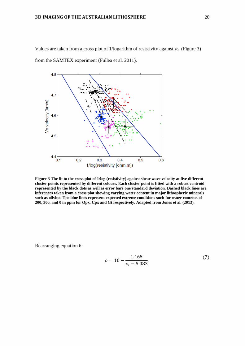
Values are taken from a cross plot of 1/logarithm of resistivity against 𝑣𝑠 (Figure 3)

from the SAMTEX experiment (Fullea et al. 2011).

Figure 3 The fit to the cross plot of 1/log (resistivity) against shear wave velocity at five different

cluster points represented by different colours. Each cluster point is fitted with a robust centroid

represented by the black dots as well as error bars one standard deviation. Dashed black lines are

inferences taken from a cross plot showing varying water content in major lithospheric minerals

such as olivine. The blue lines represent expected extreme conditions such for water contents of

200, 300, and 0 in ppm for Opx, Cpx and Gt respectively. Adapted from Jones et al. (2013).

Rearranging equation 6:

𝜌 = 10 −

1.465

𝑣𝑠 − 5.083

(7)


Applying equation 7 allows us to predict the relationship between 𝑣𝑠 and electrical

resistivity beneath Australia over a depth range of 50-150 km. Using 𝑣𝑠 values from the

AuSREM data set, the relationship was applied and resistivity was predicted at depths

of 50 km and 100 km, shown in Figure 4.

Figure 4 Map view of resistivities at depths of 50 km and 100 km with a spatial resolution of

approximately 50 km, derived from the AuSREM shear-wave velocity and the empirical

relationship equation from Jones et al. (2013). Location of cratons and basins are adapted from

Betts et al. (2002)


Results

Regions of high resistivity show a strong relationship with known geological cratons

and basins, most notably the Pilbara and Yilgarn cratons. With increasing depth from 50

to 100 km, the central Australia region becomes more resistive underneath the Arunta

and Musgrave regions. Much of the east coast remains at a consistent range of 100 to

1000 Ω.m with increasing depth. It is apparent that the highly resistive West Australian

regions correlate strongly with the observation data shown in Figure 1, in that induction

vectors in Western Australia point towards the coast and away from the highly resistive

bodies.

TESTING OBSERVATIONAL DATA

Thin Sheet Model: Methods

The thin sheet method was first developed by Price (1949) and involves to treating the

electrically conductive surface of the Earth as thin, in order to solve 3D induction

problems relating to the variations of conductance in a horizontal space, occurring in a

thin sheet above a uniform half space (Heinson and Lilley 1993). Seawater is assumed

to remain constant when compared with large geological variations in conductivity,

allowing the conductance of the ocean to become a function of depth (Heinson and

Lilley 1993). Having a sufficiently large skin depth allows a sheet of conductance to

incorporate both basins and the ocean. The thin sheet is defined by thickness h, and

local integrated conductance 𝜏(𝑥, 𝑦) at position 𝑥, 𝑦 . Beneath the thin sheet, the top

layer is considered to have conductivity 𝜍1, thickness ℎ1 and EM skin depth 𝛿 at period

T (Heinson and Lilley 1993).


Using the thin sheet method allows us to incorporate two pieces of data (where

conductivity is best known); basins and oceans. Our thin layer (the top 5 km of

Australia) contains complex variations in conductivity between 100 s and 10,000 s

(Figure 5). This allowed us to determine the surface MT and GDS responses across

Australia in a relatively high resolution thin-sheet (approximately 17 km by 17 km)

ensuring that 250 nodes were covered between 108º to 156º degrees East and 8º to 47º

degrees South.

Results

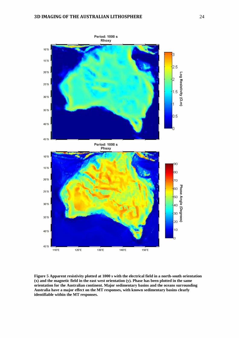
The outputs generated in the thin-sheet model shown in Figure 5 display maps of MT

responses which are consistent with characteristics at 1000 s for MT rotated data. The

apparent resistivity map in north-south orientation (x) and magnetic field orientated

east-west (y) displays conductive bodies that are represented similarly in Figure 2. It is

apparent from the thin-sheet modelling that MT responses across the country are

varying, indicating that oceans and sedimentary basins have a major effect on MT

responses. The thin-sheet model also shows that the induction vectors from the

AWAGS experiment closely resemble the modelled responses.


Figure 5 Apparent resistivity plotted at 1000 s with the electrical field in a north-south orientation

(x) and the magnetic field in the east west orientation (y). Phase has been plotted in the same

orientation for the Australian continent. Major sedimentary basins and the oceans surrounding

Australia have a major effect on the MT responses, with known sedimentary basins clearly

identifiable within the MT responses.


3D Forward Model: Methods

The 3D forward model of the Australian continent was produced using WinGlink, based

on Mackie et al. (1993) algorithms. I used induction data from the nationwide survey

conducted by AWAGS. The dimensions used in the 3D forward model were 108º E to

156º E and 8ºS to 47ºS, as well as using extra cells in order to smooth out the edges.

Resistivity of seawater was set to 0.3 Ω.m. The horizontal layer in 5 to 10 km is defined

by basic crystalline rock at 1000 Ω.m, followed by a layer from 10 to 37.5 km, defined

as the lower crust and oceanic lithosphere, at 10,000 Ω.m. Between 37.5 to 62. 5 km

resistivities have been derived from the AuSREM 50 km data set, continuing down to

150 km. Below this I have defined the asthenosphere as 100 Ω.m, the transition zone

from 400-670 km as 10 Ω.m and the lower mantle as 1 Ω.m (Figure 6). The grid node

spacing was 50 km on average.

Figure 6 Parameters set for the 3D forward model and the raw data

sets. Adapted from Wang and Lilley (1999).


Depth slices from the 3D forward model are shown in Figure 7, in comparison with

induction vectors at a period of 1000 s.

Figure 7 The 3D forward model of the Australian continent represented in map view from 0 to 5

km, 35 to 60 km, 60 to 85 km, and 85 to 110 km. Below is the observed induction vector data at a

period of 1000 s for comparison.


Results

A large percentage of Western Australia consistently has a resistivity above 4000 Ω.m.

With increasing depth, Central Australia, in particular the McArthur Basin becomes

more resistive. The surface conductance model in Figure 2 shows a conductive region

around the McArthur and Arunta regions. The forward model shows that beneath these

regions, the lithosphere becomes increasingly resistive with depth. This conforms to the

induction vectors plotted in Figure 1, with the increasing period induction vectors are

pointing away from the Arunta and McArthur regions. Finally, in the 85 to 110 km

depth slice, much of Australia appears to be highly resistive (1000 Ω.m or greater)

throughout the whole lateral extent.

From the forward model I produced a map of modelled induction vectors at a period of

1000 s (Figure 8). The synthetic induction vector trend similarly to the AWAGS

induction vectors, however there is an obvious decrease in vector size. The coastal

vectors are both similar; predominantly along the west Australian coast as well as

similar orientation, particularly throughout central Australia and inland from east

Australian coast. Major differences are obvious between the two sets of data along the

east coast of Australia, where the synthetic induction vectors are significantly smaller in

size.


Figure 8 A) The forward model synthetic induction vectors plotted at 1000 s B) AWAGS induction

vectors plotted at a period of 1000 s for comparison.


TESTING DATA

Thin-Sheet Inversion: Method

The thin-sheet inversion method has been adopted from Wang and Lilley (1999) using

the conjugate gradient relaxation method, allowing us to optimize data misfit and model

roughness. The main objective of using the thin-sheet inversion is to determine the

distribution of electrical conductance within the thin sheet layer itself (Wang and Lilley

1999).

The thin-sheet inversion was produced from AWAGS data (Figure 8). The conductance

values for the ocean surrounding Australia were kept fixed, primarily because

conductance values are mainly influenced by sea water and the conductance values can

be accurately calculated using depths from bathymetric charts. The surface grid for the

model was set to 60 by 60 cells with each cell of side length 100 km (Wang and Lilley

1999). Of the 3600 cells within the grid, 137 cells hold observed data. The ocean

conductance values were set, leaving 861 cells to be determined in the inversion

process.


Figure 9 Thin-sheet Inversion of real or in-phase induction vectors at a period of 1000 s. The

inversion reveals five regions of anomalous conductance structures which up to five times the

conductance values as the continental background. These regions have been highlighted with black

circles.

Results

The thin-sheet inversion reveals five anomalous conductive regions all over the

Australian continent. Of particular interest is the conductive area along the west

Australian coast, situated next to the resistive Pilbara craton and the conductive region

along the South Australian coast within the Gawler craton. The three other major

conductive regions are situated within known geological cratons and basins, including

the Kimberley craton and the Arunta and Musgrave regions. These regions are strongly

linked with the observational data shown in Figure 1.


DISCUSSION

Observational Data

Induction vectors are interpreted to be explained to the first order by the conduction in

the oceans and major sedimentary basins. The contrasting differences between non

sedimentary basins and the basins results in a decrease in the vector size when

compared to the coastal vectors. Over the two periods the induction vectors hold similar

trends, suggesting that with increasing period, or depth, the same deep resistivity

structures are evident. The high conductivity of the ocean ensures that the coast effect

influences the orientation and magnitude of the induction vectors along the Australian

coastline (e.g. Nam et al. 2009). The coast effect refers to the sharp electrical contrast

between the sea and the land, meaning the sea can have a substantial influence on the

GDS responses, shown in Figure 1. The influence of the coast effect means that deeper

structures within the crust and mantle may not have impacted the magnitude and

orientation of the induction vectors. Similar results were produced in Chamalaun and

Barton (1990) and Wang et al. (1997), whose induction vector plots displayed large

induction vectors along the Australian coast, although at much lower periods than those

produced in this paper.

Modelled Data

Both the surface conductance model and the thin-sheet inversion reveal similar

conductive anomalies, most notably near the Kimberley craton and Charters Towers

region. The inversion displayed conductive bodies similar to those seen in the surface

conductance model as well revealing highly conductive structures along coastal areas

which are often difficult to detect using induction vectors. Similar results can be found


in Wang et al. (1997) and Wang and Lilley (1999), whose models displayed the same

conductive bodies, in particular along the Australian coast as well as the Canning Basin

(Figure 2 and 9) . Thin-sheet modelling showed that the GDS responses across

Australia are primarily affected by the surrounding oceans and major sedimentary

basins. These results are comparable to Heinson and Lilley (1993) and Wang and Lilley

(1999). The conductive anomalies seen in figures 2 and 9 could be the result of near-

surface causes such as saline water or much deeper conduction mechanisms such as

crustal mineralisation (e.g. graphite) or deeper molten material at mantle depths. The

induction vectors in western Australia are consistent with the surface conductance

model, which shows a highly resistive region stretching for most of the state with

induction vectors influenced heavily by the highly conductive seawater, also known as

the coast effect (Simpson and Bahr 2005).

The synthetic induction vectors seen in Figure 8 establish similar trends to the AWAGS

induction vectors; however there is an obvious decrease in vector size. This suggests

that conductivity trend in the synthetic data is much weaker than those seen in the

AWAGS data. The weakening trend suggests that the forward model is missing deeper

resistivity structures which are evident within the AWAGS data.

Comparison of Observational and Modelled Data

Observation and modelled data revealed that resistivity varies throughout Australia;

regions of notably high resistivity are strongly correlated to the Western Australian

Pilbara and Yilgarn cratons. The second order effects of resistivity variations in the

deeper lithosphere are important, however the observed data become less sensitive to

these with depth. It is also clear that MT (and GDS) responses are relatively sensitive to


structures which are less than one-skin depth thick. Conductive bodies located along the

Australian coast, in particularly the west Australian coast, appear unrelated to any major

sedimentary basins.

The 3D inversion shows that there are other additional crustal conductors which cannot

be explained from sediment thickness alone and require additional conduction

mechanisms in the crust over significant depths. The synthetic induction data from the

forward model provides an ideal foundation to further develop an Australian lithosphere

resistivity structure similar to those seen in Fullea et al. (2011) and Shen et al. (2013).

CONCLUSION

In this study I have developed models of electrical resistivity using various constraints

and then tested these against known observations. It is clear that the surface

conductance accounts for most of the long-period inductive responses seen across

Australia. The second order effects of resistivity in the deeper crust are important

however the sensitivity of induction vectors or observational data is less. It is also clear

that additional crustal conductors cannot be explained from sediment thickness alone

and must require another mechanism in the crust over significant depths. Further

research could be centred on developing a continent wide magnetometer array, with a

station spacing of 100 km or less. In areas where conductive anomalies are observed,

decreasing station spacing will be required in order to produce more detailed electrical

resistivity models of the Australian lithospheric structure.


ACKNOWLEDGMENTS

I acknowledge the help of Liejun Wang and his efforts with the thin-sheet inversion. I’d

also like to thank Maptek and in particular Simon Ramsey for the imaging software and

technical assistance with this software.

I would also like to thank my primary supervisor, Professor Graham Heinson, for his

support, scientific input throughout the year and the opportunity to undertake Honours

this year. Thank you also to Stephan Thiel, Lars Krieger and Kate Robertson for their

efforts throughout the year.

REFERENCES

ARORA B. R., et al. 1999 Overview of Geomagnetic Deep Soundings (GDS) as applied in the parnaíba Basin, North-Northeast Brazil, Revista Brasileira de Geofisica, vol. 17, no. 1, pp. 41-65.

BEDROSIAN P. A. & FEUCHT D. W. 2013 Structure and tectonics of the northwestern United States from EarthScope USArray magnetotelluric data, Earth and Planetary Science Letters.

BETTS P. G., et al. 2002 Evolution of the Australian lithosphere, Australian Journal of Earth Sciences, vol. 49, no. 4, pp. 661-695.

CHAMALAUN F. & BARTON C. 1990 Comprehensive Mapping of Australia's Geomagnetic Variations, Eos, Transactions American Geophysical Union, vol. 71, no. 51, pp. 1867-1873.

CHAMALAUN F. H. & BARTON C. E. 1993 Electromagnetic induction in the Australian crust: results from the Australia-wide array of geomagnetic stations, Exploration Geophysics, vol. 24, no. 2, pp. 179-186.

CHAVE A. D. & JONES A. G. 2012 The Magnetotelluric Method: Theory and Practice. Cambridge University Press.

CHAVE A. D. & THOMSON D. J. 2004 Bounded influence magnetotelluric response function estimation, Geophysical Journal International, vol. 157, no. 3, pp. 988-1006.

EATON D. W., et al. 2009 The elusive lithosphere–asthenosphere boundary (LAB) beneath cratons, Lithos, vol. 109, no. 1, pp. 1-22.

EVANS R. L., et al. 2011 Electrical lithosphere beneath the Kaapvaal craton, southern Africa, Journal of Geophysical Research B: Solid Earth, vol. 116, no. 4.

FISHWICK S. & RAWLINSON N. 2012 3-D structure of the Australian lithosphere from evolving seismic datasets, Australian Journal of Earth Sciences, vol. 59, no. 6, pp. 809-826.

FROGTECH 2012 OZ SEEBASE


FULLEA J., MULLER M. & JONES A. 2011 Electrical conductivity of continental lithospheric mantle from integrated geophysical and petrological modeling: Application to the Kaapvaal Craton and Rehoboth Terrane, southern Africa, Journal of Geophysical Research: Solid Earth (1978–2012), vol. 116, no. B10.

HEINSON G. S., DIREEN N. G. & GILL R. M. 2006 Magnetotelluric evidence for a deep-crustal mineralizing system beneath the Olympic Dam iron oxide copper-gold deposit, southern Australia, Geology, vol. 34, no. 7, pp. 573-576.

HEINSON G. S. & LILLEY F. E. M. 1993 An application of thin-sheet electromagnetic modelling to the Tasman Sea, Physics of the Earth and Planetary Interiors, vol. 81, no. 1-4, pp. 231-251.

JONES A. G. 1999 Imaging the continental upper mantle using electromagnetic methods. pp. 57-80.

JONES A. G., EVANS R. L. & EATON D. W. 2009 Velocity–conductivity relationships for mantle mineral assemblages in Archean cratonic lithosphere based on a review of laboratory data and Hashin–Shtrikman extremal bounds, Lithos, vol. 109, no. 1, pp. 131-143.

JONES A. G., et al. 2013 Velocity-conductivity relations for cratonic lithosphere and their application: Example of Southern Africa, Geochemistry, Geophysics, Geosystems, vol. 14, no. 4, pp. 806-827.

JONES A. G., et al. 2012 Water in cratonic lithosphere: Calibrating laboratory-determined models of electrical conductivity of mantle minerals using geophysical and petrological observations, Geochemistry, Geophysics, Geosystems, vol. 13, no. 6, p. Q06010.

JONES A. G., et al. 2005 The electrical resistivity structure of Archean to Tertiary lithosphere along 3200 km of SNORCLE profiles, northwestern Canada, Canadian Journal of Earth Sciences, vol. 42, no. 6, pp. 1257-1275.

KARATO S.-I. 2010 Rheology of the Earth's mantle: A historical review, Gondwana Research, vol. 18, no. 1, pp. 17-45.

KARATO S.-I. & WU P. 1993 Rheology of the upper mantle: A synthesis, Science, vol. 260, no. 5109, pp. 771-778.

KELBERT A., EGBERT G. D. & DEGROOT-HEDLIN C. 2012 Crust and upper mantle electrical conductivity beneath the Yellowstone Hotspot Track, Geology, vol. 40, no. 5, pp. 447-450.

KENNETT B. L. N., et al. 2013 Australian seismological referencemodel (AuSREM): Mantle component, Geophysical Journal International, vol. 192, no. 2, pp. 871-887.

KENNETT B. L. N. & SALMON M. 2012 AuSREM: Australian Seismological Reference Model, Australian Journal of Earth Sciences, vol. 59, no. 8, pp. 1091-1103.

KENNETT B. L. N., et al. 2011 AusMoho: The variation of Moho depth in Australia, Geophysical Journal International, vol. 187, no. 2, pp. 946-958.

MACKIE R. L., MADDEN T. R. & WANNAMAKER P. E. 1993 Three-dimensional magnetotelluric modeling using difference equations - theory and comparisons to integral equation solutions, Geophysics, vol. 58, no. 2, pp. 215-226.

MAIER R., et al. 2007 A 3D lithospheric electrical resistivity model of the Gawler Craton, Southern Australia, Transactions of the Institutions of Mining and Metallurgy, Section B: Applied Earth Science, vol. 116, no. 1, pp. 13-21.


MILLIGAN P. R., et al. 1993 Micropulsation and induction array study near Ballarat, Victoria, Exploration Geophysics, vol. 24, no. 2, pp. 117-122.

NAM M. J., et al. 2009 Three-dimensional topographic and bathymetric effects on magnetotelluric responses in Jeju Island, Korea, Geophysical Journal International, vol. 176, no. 2, pp. 457-466.

O'REILLY S. Y. & GRIFFIN W. 2010 The continental lithosphere–asthenosphere boundary: Can we sample it?, Lithos, vol. 120, no. 1, pp. 1-13.

PANTE E. & SIMON-BOUHET B. 2013 marmap: A Package for Importing, Plotting and Analyzing Bathymetric and Topographic Data in R, PLoS ONE, vol. 8, no. 9.

PESLIER A. H., et al. 2010 Olivine water contents in the continental lithosphere and the longevity of cratons, Nature, vol. 467, no. 7311, pp. 78-81.

POMMIER A. 2013 Interpretation of Magnetotelluric Results Using Laboratory Measurements, Surveys in Geophysics, pp. 1-44.

POUDJOM DJOMANI Y. H., et al. 2001 The density structure of subcontinental lithosphere through time, Earth and Planetary Science Letters, vol. 184, no. 3-4, pp. 605-621.

PRICE A. T. 1949 The induction of electric currents in non-uniform thin sheets and shells, Quarterly Journal of Mechanics and Applied Mathematics, vol. 2, no. 3, pp. 283-310.

ROBERTS A., et al. 2008 An electromagnetic investigation of the Halls Creek Orogen. Earth and

Environmental Sciences. pp. 1-31. Adelaide University SALMON M., KENNETT B. L. N. & SAYGIN E. 2013 Australian seismological

referencemodel (AuSREM): Crustal component, Geophysical Journal International, vol. 192, no. 1, pp. 190-206.

SELWAY K. 2013 On the Causes of Electrical Conductivity Anomalies in Tectonically Stable Lithosphere, Surveys in Geophysics, pp. 1-39.

SHEN W., RITZWOLLER M. H. & SCHULTE-PELKUM V. 2013 A 3-D model of the crust and uppermost mantle beneath the Central and Western US by joint inversion of receiver functions and surface wave dispersion, Journal of Geophysical Research B: Solid Earth, vol. 118, no. 1, pp. 262-276.

SIMPSON F. & BAHR K. 2005 Practical Magnetotellurics. Cambridge University Press. THIEL S. & HEINSON G. 2013 Electrical conductors in Archean mantle-Result of plume

interaction?, Geophysical Research Letters, vol. 40, no. 12, pp. 2947-2952. VOZOFF K. 1990 Magnetotellurics: Principles and practice, Proceedings of the Indian

Academy of Sciences - Earth and Planetary Sciences, vol. 99, no. 4, pp. 441-471.

WANG D., et al. 2006 The effect of water on the electrical conductivity of olivine, Nature, vol. 443, no. 7114, pp. 977-980.

WANG L. J. & LILLEY F. E. M. 1999 Inversion of magnetometer array data by thin-sheet modelling, Geophysical Journal International, vol. 137, no. 1, pp. 128-138.

WANG L. J., LILLEY F. E. M. & CHAMALAUN F. H. 1997 Large-scale electrical conductivity structure of Australia from magnetometer arrays, Exploration Geophysics, vol. 28, no. 2, pp. 150-155.


WELSH W., BARTON C. E. & ORGANISATION A. G. S. 1996 The Australia-Wide Array of Geomagnetic Stations (AWAGS): Data Corrections. Australian Geological Survey Organisation.

Y. O'RELLY S. & GRIFFIN W. L. 1985 A xenolith-derived geotherm for southeastern australia and its geophysical implications, Tectonophysics, vol. 111, no. 1-2, pp. 41-63.

YANG J., MIN D. J. & YOO H. S. 2010 Sea effect correction in magnetotelluric (MT) data and its application to MT soundings carried out in Jeju Island, Korea, Geophysical Journal International, vol. 182, no. 2, pp. 727-740.

YOSHINO T., et al. 2009 The effect of water on the electrical conductivity of olivine aggregates and its implications for the electrical structure of the upper mantle, Earth and Planetary Science Letters, vol. 288, no. 1, pp. 291-300.

YOSHINO T., et al. 2006 Hydrous olivine unable to account for conductivity anomaly at the top of the asthenosphere, Nature, vol. 443, no. 7114, pp. 973-976.

ZHDANOV M. S., et al. 2011 Three-dimensional inversion of large-scale EarthScope magnetotelluric data based on the integral equation method: Geoelectrical imaging of the Yellowstone conductive mantle plume, Geophysical Research Letters, vol. 38, no. 8.

the 3d electrical structure of the australian lithosphere · 2017-06-28 · 3d imaging of the...

Documents