the 6-vertex model with ﬁxed boundary conditions

PoS(Solvay)012

PoS(Solvay)012

The 6-vertex model with fixed boundary conditions.

Nicolai Reshetikhin ∗†Department of mathematics, University of California, Berkeley, CA 94720, USAE-mail: [email protected]

Konstantin PalamarchukDepartment of mathematics, University of California, Berkeley, CA 94720, USAE-mail: [email protected]

We study the 6-vertex model with fixed boundary conditions. In the thermodynamical limit there is a

formation of the limit shape. We collect most of the known results about the analytical properties of

the free energy of the model as the function of electric fields and study the asymptotical behavior near

singularities. We also study the asymptotic of limit shapes and the structure of correlation functions in the

bulk

Bethe Ansatz: 75 years laterOctober 19-21 2006,Brussels, Belgium

∗Speaker.†A footnote may follow.

c© Copyright owned by the author(s) under the terms of the Creative Commons Attribution-NonCommercial-ShareAlike Licence. http://pos.sissa.it/

mailto:[email protected]�

mailto:[email protected]�

PoS(Solvay)012

PoS(Solvay)012

The6-vertex model Nicolai Reshetikhin

1. Introduction

*

Ising and dimer models were among the first models in two-dimensional statistical mechanics for wherethe partition function and for some of the correlation functions were computed explicitly in terms of Pfaffiansof certain matrices. For this reason both of these models can be regarded as theories of Gaussian discretetwo dimensional fermi field. The Ising model was solved by Onsager and for dimer models the Pfaffiansolution was found by Kasteleyn.

The6-vertex model, a particular case of which is the ice model is interesting for a number of reasons.Physically, it is a model of ferro- and antiferro- electricity. It has many equivalent reformulations, oneof them (which we will use) describe the 6-vertex configurations on a planar connected simply connectedregion in terms of stepped surfaces. One of the combinatorial reformulations of the 6-vertex model forspecific value of parameters [Kup] is related to alternating sign matrices [Bres].

The 6-vertex model generalizes dimer models and can be regraded as the theory of Gaussian discretefermions with four fermionic interaction. The partition function of the 6-vertex model with periodic bound-ary conditions was computed in [Lieb] using the Bethe Ansatz method.

The computation of correlation functions in the6-vertex model is highly non-trivial and to the largedegree is still a challenge. There are two known approaches to this problem based on the internal symmetryof the model, i.e. on the representation theory of quantum affine algebras. First approach is based ondeterminantal formulae for certain matrix elements [KBI ]. For some recent results based on this method see[BPZ] and [CP]. The second approach is based on form-factor formulae derived in [Sm]. For an overviewof this approach see [JM] and for the latest results see [BJMST].

The 6-vertex model on a planar simply regions can be reformulated as the theory of random steppedsurfaces. A configuration of arrows in a 6-vertex model can be interpreted as a configuration of paths whichcan be viewed as level corves of aheight functiondefining a stepped surface. Gibbs measure on 6-vertexconfigurations define a Gibbs measure on stepped surfaces.

For certain class of such Gibbs measures, random surfaces in the thermodynamical limit develop thelimit shape phenomenon [Shef] also known as the acric circle phenomenon [CEP]. It means that on macro-scopical scale the random surface becomes deterministic. The fluctuations remain at smaller scale and thestructure of fluctuations may change depending on how singular the limit shape is at this point. The limitshape phenomenon is studied in details in dimer models [KO].

The numerical results from [AR][SZ] show how limit shapes develop in a 6-vertex model with domainwall boundary conditions. In this paper we will focus on the limit shape phenomenon for the 6-vertex modelon a planar connected simply connected regions with fixed boundary conditions. Computing the limit shapeinvolves two steps.

Step one is the derivation of the formula for the free energy of the 6-vertex model as a function of mag-netic fields. Unlike the partition function of dimer models, the free energy can not be computed explicitly.However, it can be written in terms of the solution to a linear integral equation. Many analytical properties of

2

PoS(Solvay)012

PoS(Solvay)012


the partition function are known but scattered in the literature, see for example [Yang][Yang1][SY][SY1][LW][BS][Nold][NK]. We collected most of them in the section3 together with some new results.

Step two is to derive and solve the variational principle which determine the limit shape for givenboundary conditions. The free energy of the model as a function of magnetic fields determine the functionalin the variational problem. Such variational problem was first introduced for dimer models in [CKP]. Theidea of using this variational problem in the 6-vertex first appeared in [Z1] where some interesting partialresults were obtained for correlation functions in the bulk of the limit shape.

The structure of fluctuations near the limit shape is determined by the asymptotical behavior of corre-lation functions at smaller scales. We will discuss this problem for the 6-vertex model in the last section.

Finally let us mention the special case of domain wall boundary conditions. These boundary conditionsfirst appeared in the computation of norms of Bethe vectors [Kor]. The remarkable fact about them is thatthe partition function of the 6-vertex model with these boundary conditions can be written as a determinant[Ize]. Another remarkable fact is that exactly these boundary conditions relate the 6-vertex model withalternating sign matrices [Kup]. The large volume asymptotic of the partition function of the 6-vertex modewith these boundary conditions was computed in [KZ][Z].

Here is the outline of the paper. In the first two sections we recall some basic facts about the6-vertexmodel, about its reformulation it in terms of height functions, and about the thermodynamical limit in themodel. The third section contains the description of the free energy per site for as the function of electricfields in thermodynamical limit for periodic boundary conditions. Some asymptotical behaviors of the freeenergy are computed in section 4. This section is a combination of an overview and original results. Insection 5 we study the asymptotical behavior of the limit shapes near the "freezing point". In the last sectionwe discuss fluctuations.

We thank C. Evans, R. Kenyon, A. Okounkov, and S. Sheffield for interesting discussions. The workof N.R. was supported by the NSF grant DMS 0307599, by the Niels Bohr initiative at Aarhus University,by the Humboldt foundation and by the CRDF grant RUMI1-2622 The work of K.P. was supported by theNSF RTG grant and DMS 0307599.

2. The6-Vertex Model

2.1 The6-vertex model

First, let us fix the notation. A squareN×M grid LN,M is a graph with4- and1-valent vertices embeddedinto R2 such that4-valent vertices are located at points(n,m), n = 0,1, . . . ,N−1,m= 0,1, . . . ,M−1 (seeFig. 2) and1-valent vertices are located at(−1,m),(N,m),m= 0,1, . . . ,M−1 and at(n,−1),(n,M−1),n=0,1, . . . ,N−1. An edge connecting two4-valent vertices is called aninner edge and an edge connecting a4-valent vertex with a1-valent vertex is called anouteredge.

States of the6-vertex model onLN,M are configurations of arrows assigned to each edge (i.e. orienta-tions ofLN,M). They satisfy the ice rule: at any vertex the number of incoming arrows should be equal tothe number of outgoing arrows. Six possible configurations at a vertex are shown on Fig.1. Configurationsof arrows on boundary edges are called boundary conditions.

3

PoS(Solvay)012

PoS(Solvay)012


Each configuration of arrows on the lattice can be equivalently described as the configuration of “thin”and “thick” edges or empty and occupied edges shown on Fig.1. There should be an even number of thickedges at each vertex as a consequence of the ice rule. The thick edges form paths. We assume that paths donot intersect (two paths may meet at ana1-vertex). So, equivalently, configurations of the6-vertex modelcan be regarded as configurations of paths satisfying the rules from Fig.1.

To each configuration of arrows on edges adjacent to a vertex we assign a Boltzmann weight, which wedenote by the same letters. The physical meaning of a Boltzmann weight isexp(−E

T ), whereE is the energyof a state andT is the temperature (in the appropriate units). Thus, all numbersa1, a2, b1, b2, c1, andc2

should be positive.Choosing the scale such thatT = 1, it is natural to write Boltzmann weights in the exponential form.

a1 = e−E1+H+V , a2 = e−E1−H−V ,

b1 = e−E2+H−V , b2 = e−E2−H+V ,

c1 = e−E3, c2 = e−E3,

whereE1, E2, andE3 are dimensionless interaction energies of arrows at different types of vertices, andH andV are dimensionless horizontal and vertical components of the magnetic field, respectively. In thisinterpretation arrows are spins interacting with the magnetic field. We setc1 = c2 because for the types ofboundary conditions we will consider the difference between the number ofc1-vertices andc2 vertices is thesame for all states and, therefore, the probability does not depend on the ratioc1/c2.

We also use the standard notation

a = e−E1, b = e−E2, c = e−E3.

These are the weights of the model when there is no magnetic field.The weight of a state is the product of weights of vertices in the state. The weight of a state onLN (up

to a constant factor) can be written in terms of energies and magnetic fields as

exp(−E1N(a)−E2N(b)−E3N(c)+H2

N(hor)+V2

N(ver))

whereN(a) is the total number ofa-vertices,N(b) is the total number ofb-vertices,N(c) is the total numberof c-vertices,N(hor) is the total number of horizontal edges occupied by paths, andN(vert) is the totalnumber of vertical edges occupied by paths.

The partition function is the sum of weights of all states of the model

Z = ∑states

∏vertices

w(vertex),

wherew(vertex) is one of the weights from Fig.1.Weights define the probabilistic measure on the set of states of the6-vertex model. The probability of

a state is given by the ratio of the weight of the state to the partition function of the model

P(state) = ∏verticesw(vertex)Z

.

4

PoS(Solvay)012

PoS(Solvay)012


a1

b1

a2

b2

c1 c

2

Figure 1: The6 types of vertices and the corresponding thin and thick edges configurations

This is the Gibbs measure of the6-vertex model.

Let us define the characteristic function of an edgeeas

σe(state) =

{1, if e is occupied by a path;0, otherwise

A local correlation function is the expectation value of the product of such characteristic functions:

〈σe1σe2..σen〉= ∑states

P(state)n

∏i=1

σei (state)

2.2 Boundary Conditions

2.2.1

Let us fix arrows (or, equivalently, think edges) on outer edges ofLN,M. States in the 6-vertex withthe same configurations of arrows on the boundary are called states withfixedboundary conditions. Thedifference between two such states can occur only at inner edges.

The space of states with fixed boundary conditions is empty unless the boundary values satisfy theice rule: the total number of incoming arrows on the boundary edges should be equal to the total numberof outgoing arrows. In the path formulation this means that the number of paths through North and Westboundaries should be equal to the number paths through the South and East boundaries.

An example of such boundary conditions is the domain wall (DW) boundary conditions. For the DWboundary conditions the arrows on the boundary of the lattice are going into the lattice at the top and bottomof the lattice and are going out of the lattice at the right and left of it. A configuration of paths on a5×5lattice with DW boundary conditions is presented on Fig.2.

5

PoS(Solvay)012

PoS(Solvay)012


Figure 2: A possible configuration of paths on a5×5 square grid for the DW boundary conditions

Notice that the differences

na = n(a1)−n(a2), nb = n(b1)−n(b2), nc = n(c2)−n(c1)

are the same for all configurations with given fixed boundary conditions. Heren(x) is the total number ofvertices of typex = ai ,bi ,ci in the configuration.

In particular, the partition function for fixed boundary conditions trivially depends on magnetic fields:

Z(a1,a2,b1,b2,c1,c2) = e(Hnb+Vna)(

c2

c1

) nc2

Z(a,a,b,b,c,c)

In this paper we will focus on the6-vertex model with fixed boundary conditions.

2.2.2

Another important type of boundary conditions are theperiodic boundary conditions. In this casethe edges at opposite sides ofLN,M are identified so that the configuration of arrows on the left and rightboundary is the same as well as the configuration of arrows on the top and bottom boundary.

The 6-vertex model with periodic boundary conditions is an example of an “integrable” (solvable)model in statistical mechanics and has been studied extensively, see [Bax],[LW] and references therein. Inparticular, it means that the row-to-row transfer-matrix of the model can be diagonalized by the Bethe ansatz.

2.3 The Height Function

By outer faceswe mean unit squares centered at(−12,m), (N− 1

2,m), with m= −12, 1

2, . . . ,M− 12 and

(n,−12), (n,N− 1

2), with n=−12, 1

2, . . . ,N− 12. Each corner outer face has two edges in their boundary, other

outer faces have three edges in their boundary.

6

PoS(Solvay)012

PoS(Solvay)012


A height functionh is an integer-valued function on the facesFN of the gridLN (including the outerfaces), which is

• zero at the southwest corner of the grid,

• non-decreasing when going up or right,

• if f1 and f2 are neighboring faces, then|h( f1)−h( f2)| ≤ 1.

Theboundary valueof the height function is its restriction to the “outer faces”. Denote the set of outerfaces by∂FN. Given a functionh(0) on ∂FN denoteH (h(0)) the space of all height functions with theboundary valueh(0).

If we enumerate faces by the coordinates of their centers the height function can be regarded as(N +1)× (M +1) matrix with non-negative entries.

It is clear that there is a bijection between states of the6-vertex model with fixed boundary conditionsand height functions with fixed boundary values.

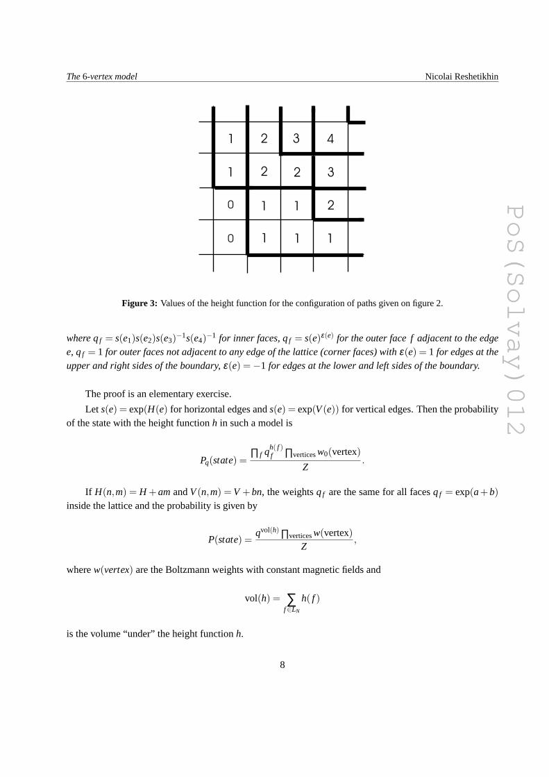
Indeed, given a height function consider its “level curves”, i.e. paths on the gridLN, where the heightfunction changes its value by1, see Fig.3. Clearly, this defines a state for the6-vertex model onLN withboundary conditions determined by the boundary values of the height function.

On the other hand, given a state in the6-vertex model, consider the corresponding configuration ofpaths. It is clear that there is a unique height function whose level curves are these paths and which satisfiesthe conditionh = 0 at the southwest corner.

It is clear that this correspondence is a bijection.There is a natural partial order on the set of height functions with given boundary values. One function

is bigger then the other if it is entirely above the other. There exist the minimumhmin and the maximumhmax height functions such thathmin ≤ h≤ hmax for all height functionsh.

Thus, we can consider the6-vertex model as a theory of fluctuating discrete surfaces constrained be-tweenhmax andhmin. Each surface occurs with probability given by the Boltzmann weights of the6-vertexmodel.

2.4 The inhomogeneous6-vertex model and volume weights

In the inhomogeneous6-vertex model the Boltzmann weights depend on the edge. Thus, we have6N2

parametersai(m,n), bi(m,n), andci(m,n).Let us assume that the inhomogeneity is only in magnetic fields, i.e. weightsa,b, andc do not change

from edge to edge, but the magnetic fieldsH(e), V(e) do.Let {P} be the collection of paths corresponding to a state in the6-vertex model and{h( f )} be the

corresponding height function.

Proposition 2.1. Let us assign weightss(e) to the edges of the lattice and1 to the outer edges, then

∏f

qh( f )f = ∏

P∏e∈P

s(e)

7

PoS(Solvay)012

PoS(Solvay)012


0

0

1 2

1

1

1

1

11

2

22

3 4

3

Figure 3: Values of the height function for the configuration of paths given on figure 2.

whereqf = s(e1)s(e2)s(e3)−1s(e4)−1 for inner faces,qf = s(e)ε(e) for the outer facef adjacent to the edgee, qf = 1 for outer faces not adjacent to any edge of the lattice (corner faces) withε(e) = 1 for edges at theupper and right sides of the boundary,ε(e) =−1 for edges at the lower and left sides of the boundary.

The proof is an elementary exercise.

Let s(e) = exp(H(e) for horizontal edges ands(e) = exp(V(e)) for vertical edges. Then the probabilityof the state with the height functionh in such a model is

Pq(state) =∏ f qh( f )

f ∏verticesw0(vertex)

Z.

If H(n,m) = H +amandV(n,m) = V +bn, the weightsqf are the same for all facesqf = exp(a+b)inside the lattice and the probability is given by

P(state) =qvol(h) ∏verticesw(vertex)

Z,

wherew(vertex) are the Boltzmann weights with constant magnetic fields and

vol(h) = ∑f∈LN

h( f )

is the volume “under” the height functionh.

8

PoS(Solvay)012

PoS(Solvay)012


3. The thermodynamic limit

3.1 Stabilizing sequence of fixed boundary conditions

3.1.1

Let a = M/N. We place the gridLN,M inside of the rectangleD = {(x,y)| 0≤ x≤ 1,0≤ y≤ a} so thatthe vertices of the grid are the points with coordinates( n

N+1, mN+1) wheren = 1, . . . ,N, m= 1, . . . ,M.

We recall that a height function is a monotonic integer-valued function on the faces of the grid, whichsatisfies Lipshitz condition (it changes at most by1 on any two adjacent faces). The height function canbe regarded as a function on the centers of the faces of the grid, i.e on(n− 1/2,m− 1/2), wheren =0, . . . ,N + 1, m = 0,1, . . . ,M + 1. The points(1

2,m− 12), (N + 1

2,m− 12), (n− 1

2, 12), and(n− 1

2,M + 12),

wheren = 0, . . . ,N+1, m= 0, . . . ,M +1 correspond to the “outer” faces ofLN,M.We introduce the normalized height function as a piecewise linear function on the unit square with the

valuehnorm

N (x,y) =1N

hN(n,m).

for nN+1 ≤ x≤ n+1

N+1 and mN+1 ≤ y≤ m+1

N+1. HerehN(n,m) is a height function onLN,M. Normalized heightfunctions are nondecreasing inx andy directions and they satisfy:

h(x,y)−h(x′,y′)≤ x−x′+y−y′. (3.1)

if x≥ x′ andy≥ y′.The boundary value of the normalized height function defines a piece-wise constant monotonic function

on each side of the region which changes by±1/N or do not change between two neighboring boundarysites.

Denote the space of such normalized height functions with the boundary valueh0 by LN,M(h0).There is a natural partial ordering on the set of all normalized height functions with given boundary

values descending from the partial order on height functions:h1 ≥ h2 if h1(x) ≥ h2(x) for all x ∈ D. Wedefine the operations

h1∨h2 = minx∈D(h1(x),h2(x)), h1∧h2 = maxx∈D(h1(x),h2(x)),

It is clear thath1∧h2 ≥ h1,h2 ≥ h1∨h2

It is also clear that in this partial order there is unique minimal and unique maximal height functions, whichwe denote byhmin

N andhmaxN , respectively.

A sequence of stabilizing fixed boundary conditionsis a sequence of functionsh(N)0 which are boundary

values of a normalized height function, and which converges ??? asN→∞ to a functionφ0 on the boundary Topologyof D which is non-decreasing alongx andy direction,φ(0,0) = 0, and satisfies the condition:

φ(x,y)−φ(x′,y′)≤ x−x′+y−y′ (3.2)

9

PoS(Solvay)012

PoS(Solvay)012


We will call the functionφ0 the boundary condition for the domainD (or simply the boundary condi-tion). Any function onD which satisfies (3.2), which is non-decreasing inx andy directions, and coinsidewith φ0 at the boundary is called aheight function onD with boundary conditionφ0.

Among all possible boundary conditionsφ0 we will distinguish piecewise linear boundary conditionswith the slope0 or 1 along the coordinate axes. We will call these boundary valuescritical . It is clear thatany boundary conditions can be approximated critical boundary conditions.

3.2 The thermodynamic limit

If q is fixed and is not equal to1 in the large volume limit, the system will be in a neighborhood of theminimal height function forq < 1 and in the neighborhood of the maximal height function forq > 1. Oneshould expect that the partition function and local correlation functions will have finite limit.

Whenq = exp( λN) for someλ , one should expect the existence of the limit shape. We will study this

limit in Section7.

3.3 Gibbs measures with fixed slope

Definition 3.1. The Gibbs measure of the6-vertex model on an infinite lattice has the slope(h,v) if

limk→∞

<h(n+k,m)−h(n,m)

k>= h

and

limk→∞

<h(n,m+k)−h(n,m)

k>= v

It is clear from the definition of the height function that the slope should satisfy conditions0≤ h,v≤ 1.

The slope is simply the average number of horizontal and vertical edges occupied by paths per length.

The important corollary of the result of [Shef] is that, when a gradient Gibbs measure satisfies certainconvexity conditions, there exists a unique translationally invariant measure. This implies that for the6-vertex model one should expect the uniqueness of such a measure for the generic slope.

Translationally invariant measures can be obtained by taking the thermodynamic limit of the 6-vertexmodel with magnetic fields on a torus. Then the slope is the Legendre conjugate to magnetic fields.

h = limN,M→∞

〈σe〉= limN,M→∞

〈N(hor)N

〉= limN,M→∞

12NM

∂ logZ∂H

+12

for a horizontaleand

v = limN.M→∞

〈σe〉= limN,M→∞

〈N(ver)N

〉= limN,M→∞

12NM

∂ logZ∂V

+12

for a verticale.

10

PoS(Solvay)012

PoS(Solvay)012


4. The thermodynamic limit of the 6-vertex model for the periodic boundary conditions

The free energy per site in the thermodynamic limit is

f =− limN,M→∞

log(ZN,M)NM

whereZN,M is the partition function with the periodic boundary conditions on the rectangular gridLN,M. Itis a function of the Boltzmann weights and magnetic fields.

Remark 1. Normally, it is expected that the free energy is not identically zero. Physically, this means thatthe “excitations” have the characteristic length which is much smaller than the characteristic length of thesystem. In some cases the free energy is identically zero, then one expects that a typical excitation will becomparable with the size of the system.

For genericH andV the 6-vertex model in the thermodynamic limit has the translationally invariantGibbs measure with the slope(h,v):

h =−12

∂ f∂H

+12, v =−1

2∂ f∂V

+12. (4.1)

The parameter

∆ =a2 +b2−c2

2ab.

defines many characteristics of the6-vertex model in the thermodynamic limit.

4.1 The phase diagram for∆ > 1

The weightsa, b, andc in this region satisfy one of the two inequalities, eithera > b+c or b > a+c.If a > b+c, the Boltzmann weightsa, b, andc can be parameterized as

a = r sinh(λ +η),b = r sinh(λ ),c = r sinh(η) (4.2)

with λ ,η > 0.If a+c < b, the Boltzmann weights can be parameterized as

a = r sinh(λ −η),b = r sinh(λ ),c = r sinh(η) (4.3)

with 0 < η < λ .For both of these parametrization of weights∆ = cosh(η).The phase diagram of the model fora> b+c (and, therefore,a> b) is shown on Fig.5 and forb> a+c

(and, therefore,a < b) on Fig.6.When magnetic fields(H,V) are in one of the regionsAi ,Bi of the phase diagram, the system in the

thermodynamic limit has the translationally invariant Gibbs measure supported on the corresponding frozen

11

PoS(Solvay)012

PoS(Solvay)012


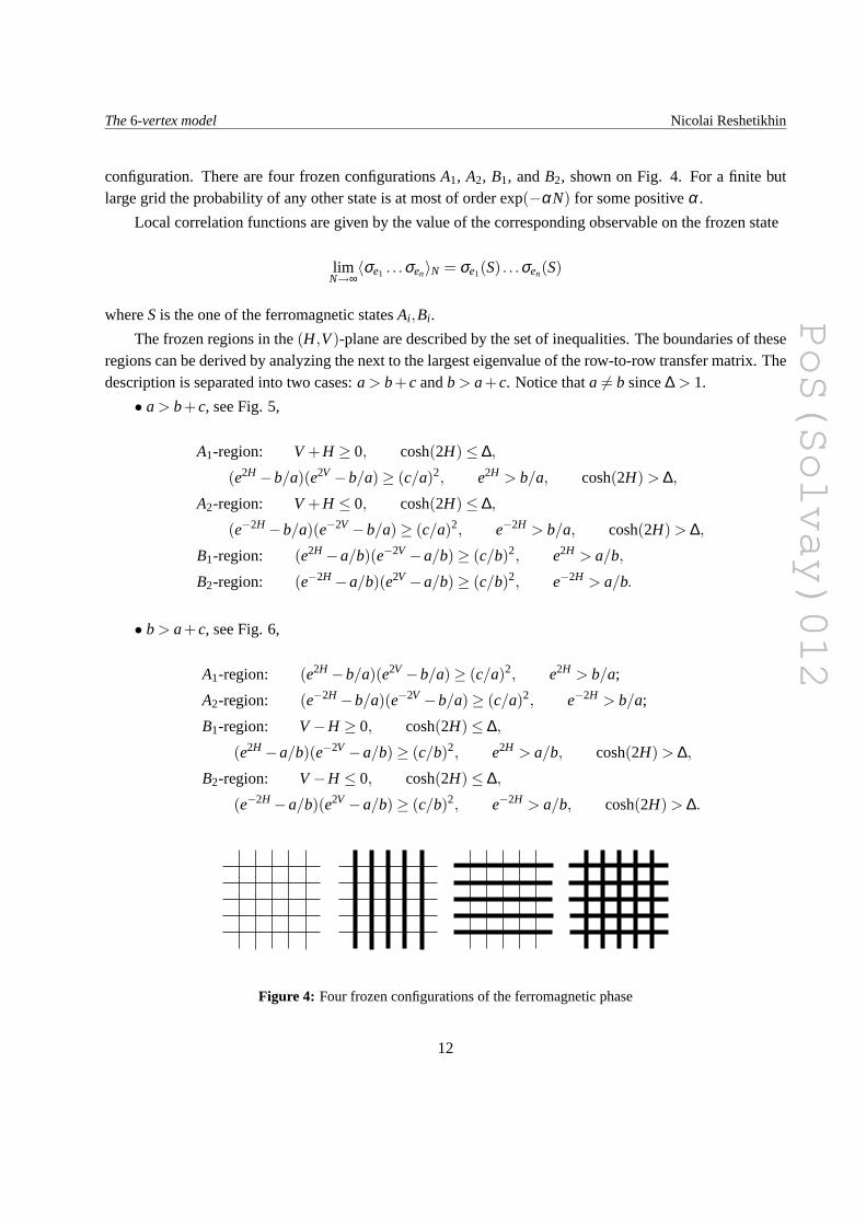
configuration. There are four frozen configurationsA1, A2, B1, andB2, shown on Fig.4. For a finite butlarge grid the probability of any other state is at most of orderexp(−αN) for some positiveα.

Local correlation functions are given by the value of the corresponding observable on the frozen state

limN→∞

〈σe1 . . .σen〉N = σe1(S) . . .σen(S)

whereS is the one of the ferromagnetic statesAi ,Bi .

The frozen regions in the(H,V)-plane are described by the set of inequalities. The boundaries of theseregions can be derived by analyzing the next to the largest eigenvalue of the row-to-row transfer matrix. Thedescription is separated into two cases:a > b+c andb > a+c. Notice thata 6= b since∆ > 1.

• a > b+c, see Fig.5,

A1-region: V +H ≥ 0, cosh(2H)≤ ∆,

(e2H −b/a)(e2V −b/a)≥ (c/a)2, e2H > b/a, cosh(2H) > ∆,

A2-region: V +H ≤ 0, cosh(2H)≤ ∆,

(e−2H −b/a)(e−2V −b/a)≥ (c/a)2, e−2H > b/a, cosh(2H) > ∆,

B1-region: (e2H −a/b)(e−2V −a/b)≥ (c/b)2, e2H > a/b,

B2-region: (e−2H −a/b)(e2V −a/b)≥ (c/b)2, e−2H > a/b.

• b > a+c, see Fig.6,

A1-region: (e2H −b/a)(e2V −b/a)≥ (c/a)2, e2H > b/a;

A2-region: (e−2H −b/a)(e−2V −b/a)≥ (c/a)2, e−2H > b/a;

B1-region: V−H ≥ 0, cosh(2H)≤ ∆,

(e2H −a/b)(e−2V −a/b)≥ (c/b)2, e2H > a/b, cosh(2H) > ∆,

B2-region: V−H ≤ 0, cosh(2H)≤ ∆,

(e−2H −a/b)(e2V −a/b)≥ (c/b)2, e−2H > a/b, cosh(2H) > ∆.

Figure 4: Four frozen configurations of the ferromagnetic phase

12

PoS(Solvay)012

PoS(Solvay)012


-1

-0.5

0

0.5

1

-1 -0.5 0.5 1

B2

A1

B1

A2

D1

D2

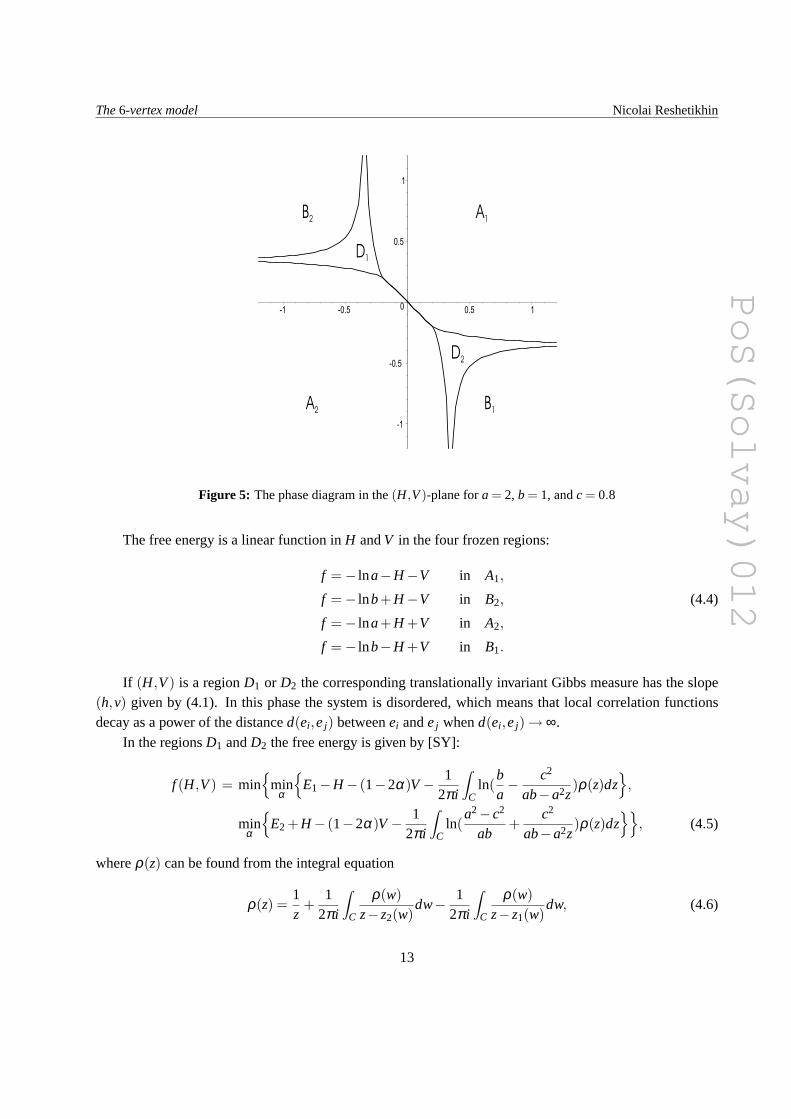
Figure 5: The phase diagram in the(H,V)-plane fora = 2, b = 1, andc = 0.8

The free energy is a linear function inH andV in the four frozen regions:

f =− lna−H−V in A1,

f =− lnb+H−V in B2, (4.4)

f =− lna+H +V in A2,

f =− lnb−H +V in B1.

If (H,V) is a regionD1 or D2 the corresponding translationally invariant Gibbs measure has the slope(h,v) given by (4.1). In this phase the system is disordered, which means that local correlation functionsdecay as a power of the distanced(ei ,ej) betweenei andej whend(ei ,ej)→ ∞.

In the regionsD1 andD2 the free energy is given by [SY]:

f (H,V) = min{

minα

{E1−H− (1−2α)V− 1

2π i

∫

Cln(

ba− c2

ab−a2z)ρ(z)dz

},

minα

{E2 +H− (1−2α)V− 1

2π i

∫

Cln(

a2−c2

ab+

c2

ab−a2z)ρ(z)dz

}}, (4.5)

whereρ(z) can be found from the integral equation

ρ(z) =1z

+1

2π i

∫

C

ρ(w)z−z2(w)

dw− 12π i

∫

C

ρ(w)z−z1(w)

dw, (4.6)

13

PoS(Solvay)012

PoS(Solvay)012


-1

-0.5

0

0.5

1

-1 -0.5 0.5 1

A1

B1

A2

B2

D2

D1

Figure 6: The phase diagram in the(H,V)-plane fora = 1, b = 2, andc = 0.8

in which

z1(w) =1

2∆−w, z2(w) =− 1

w+2∆.

ρ(z) satisfies the following normalization condition:

α =1

2π i

∫

Cρ(z)dz.

The contour of integrationC (in the complexz-plane) is symmetric with respect to the conjugationz→ z̄, isdependent onH (see AppendixB) and is defined by the condition that the formρ(z)dzhas purely imaginaryvalues on the vectors tangent toC:

Re(ρ(z)dz)∣∣∣z∈C

= 0.

The formula (4.5) for the free energy follows from the Bethe Ansatz diagonalization of the row-to-row transfer-matrix. Its derivation is outlined in AppendixB. It relies on a number of conjectures that aresupported by numerical and analytical evidence and in physics are taken for granted. However, there is norigorous proof.

There are two points where three phases coexist (two frozen and one disordered phase). These pointsare calledtricritical . The angleθ between the boundaries ofD1 (or D2) at a tricritical point is given by

cos(θ) =c2

c2 +2min(a,b)2(∆2−1).

14

PoS(Solvay)012

PoS(Solvay)012


The existence of such points makes the6-vertex model (and its degeneration known as the5-vertex model[HWKK]) remarkably different from dimer models [KOS] where generic singularities in the phase diagramare cusps. Physically, the existence of singular points where two curves meet at the finite angle manifeststhe presence of interaction in the6-vertex model.

Notice that when∆ = 1 the phase diagram of the model has a cusp at the pointH = V = 0. This is thetransitional point between the region∆ > 1 and the region|∆|< 1 which is described below.

4.2 The phase diagram|∆|< 1

In this case, the Boltzmann weights have a convenient parameterization by trigonometric functions.When1≥ ∆≥ 1

a = r sin(λ − γ),b = r sin(λ ),c = r sin(γ),

where0≤ γ ≤ π/2, γ ≤ λ ≤ π, and∆ = cosγ.

When0≥ ∆≥−1

a = r sin(γ−λ ),b = r sin(λ ),c = r sin(γ),

where0≤ γ ≤ π/2, π− γ ≤ λ ≤ π, and∆ =−cosγ.

The phase diagram of the6-vertex model with|∆|< 1 is shown on Fig.7. The phasesAi ,Bi are frozenand identical to the frozen phases for∆ > 1. The phaseD is disordered. For magnetic fields(H,V) theGibbs measure is translationally invariant with the slope(h,v) = ( ∂ f (H,V)

∂H , ∂ f (H,V)∂V ).

The frozen phases can be described by the following inequalities:

A1-region: (e2H −b/a)(e2V −b/a)≥ (c/a)2, e2H > b/a,

A2-region: (e−2H −b/a)(e−2V −b/a)≥ (c/a)2, e−2H > b/a,

B1-region: (e2H −a/b)(e−2V −a/b)≥ (c/b)2, e2H > a/b, (4.7)

B2-region: (e−2H −a/b)(e2V −a/b)≥ (c/b)2, e−2H > a/b.

The free energy function in the frozen regions is still given by the formulae (4.5). The first derivativesof the free energy are continuous at the boundary of frozen phases, The second derivative is continuous inthe tangent direction at the boundary of frozen phases and is singular in the normal direction.

It is smooth in the disordered region where it is given by (4.5) which, as in case∆ > 1 involves asolution to the integral equation (4.6). The contour of integration in (4.6) is closed for zero magnetic fieldsand, therefore, the equation (4.6) can be solved explicitly by the Fourier transformation [Bax] .

The 6-vertex Gibbs measure with zero magnetic fields converges in the thermodynamic limit to thesuperposition of translationally invariant Gibbs measures with the slope(1/2,1/2). There are two suchmeasures. They correspond to the double degeneracy of the largest eigenvalue of the row-to-row transfer-matrix [Bax].

There is a very interesting relationship between the6-vertex model in zero magnetic fields and thehighest weight representation theory of the corresponding quantum affine algebra. The double degeneracy

15

PoS(Solvay)012

PoS(Solvay)012


-2

-1

0

1

2

-2 -1 1 2

B2

A1

B1

A2

D

V

H

Figure 7: The phase diagram in the(H,V)-plane fora = 1, b = 2, andc = 2

of the Gibbs measure with the slope(1/2,1/2) corresponds to the fact that there are two integrable irre-ducible representations of̂sl1 at level one. Correlation functions in this case can be computed usingq-vertexoperators [JM]. For latest developments see [BJMST].

4.3 The phase diagram∆ <−1

4.3.1 The phase diagram

The Boltzmann weights for these values of∆ can be conveniently parameterized as

a = r sinh(η−λ ),b = r sinh(λ ),c = r sinh(η), (4.8)

where0 < λ < η and∆ =−coshη .The Gibbs measure in thermodynamic limit depends on the value of magnetic fields. The phase diagram

in this case is shown on Fig.8 for b/a > 1. In the parameterization (4.8) this correspond to0 < λ < η/2.Whenη/2 < λ < η the4-tentacled “amoeba” is tilted in the opposite direction as on Fig.5. When(H,V)is in one of theAi ,Bi regions in the phase diagram the Gibbs measure is supported on the correspondingfrozen configuration, see Fig.4.

16

PoS(Solvay)012

PoS(Solvay)012


-3

-2

-1

0

1

2

3

-3 -2 -1 1 2 3

B2

A1

B1

A2

D

A

V

H

Figure 8: The phase diagram in the(H,V)-plane fora = 1, b = 2, andc = 6

The Ai ,Bi regions on the phase diagram are defined by inequalities (4.7). The free energy in theseregions is linear and is given by (4.5).

If (H,V) is in the regionD, the Gibbs measure is the translationally invariant measure with the slope(h,v) determined by (4.1). The free energy in this case is determined by solutions to the linear integralequation (4.6) and is given by the formula (4.5).

If (H,V) is in the regionA, the Gibbs measure is the superposition of two Gibbs measures with the slope(1/2,1/2). In the limit∆→−∞ these two measures degenerate to two measures supported on configurationsC1,C2, respectively, shown on Fig.9. For a finite∆ the support of these measures consists of configurationswhich differ fromC1 andC2 in finitely many places on the lattice.

We notice that any two configurations lying in the support of each of these Gibbs measures can beobtained fromC1 or C2 via flipping the path at a vertex “up” or “down” as it is shown on Fig.10 finitelymany times. It is also clear that it takes infinitely many flips to go fromC1 to C2.

The6-vertex model in the phaseA is disordered and is also noncritical.Here non-criticality means that the local correlation function〈σei σej 〉 decays asexp(−αd(ei ,ej)) with

some positiveα as the distanced(ei ,ej) betweenei andej increases to infinity.The free energy in theA-region can be explicitly computed by solving the equation (4.6) via the Fourier

17

PoS(Solvay)012

PoS(Solvay)012


transform [Bax].

4.3.2 The antiferromagnetic region

This boundary of the antiferromagnetic regionA can be derived similarly to the boundaries of theferromagnetic regionsAi andBi by analyzing next to the largest eigenvalue of the row-to-row transfer-matrix.The difference is that for the regionA the largest eigenvalue will correspond ton = N/2 and to compute itwe should use the solution to the integral equation (4.6) in the case when the contour of integration is closed.

This computation was done in [SY], [LW]. The result is a simple closed curve, which can be describedparameterically as

H(s) = Ξ(s), V(s) = Ξ(η−θ0 +s),

whereΞ(ϕ) = cosh−1

( 1

dn(Kπ ϕ |1−ν)

),

|s| ≤ 2η ,

and

eθ0 =1+max(b/a,a/b)eη

max(b/a,a/b)+eη .

The parameterν is defined by the equationηK(ν) = πK′(ν), where

K(ν) =∫ π/2

0(1−ν sin2(θ))−1/2dθ K′(ν) =

∫ π/2

0(1− (1−ν)sin2(θ))−1/2dθ .

The curve is invariant with respect to the reflections(H,V)→ (−H,−V) and(H,V) → (V,H) sincethe functionΞ satisfies the identities

Ξ(ϕ) =−Ξ(−ϕ), Ξ(η−ϕ) = Ξ(η +ϕ).

This function is also4η-periodic:Ξ(4η +ϕ) = Ξ(ϕ).

Figure 9: Two most probable configurations in the antiferromagnetic phase.

18

PoS(Solvay)012

PoS(Solvay)012


up

down

Figure 10: The elementary up and down fluctuations in the antiferromagnetic phase.

Proposition 4.1. The boundary of the antiferromagnetic region is a real algebraic curve ineH andeV givenby

((1−ν cosh2V0)cosh2H +sinh2V0− (1−ν)coshV0coshH coshV

)2=

(1−ν cosh2V0)sinh2V0cosh2V sinh2H(1−ν cosh2H), (4.9)

whereV0 is the positive value ofV on the curve whenH = 0. Notice thatν depends on the Boltzmannweightsa,b,c only throughη .

Proof. The parametric description of the boundary curve implies that

dn(Kπ

s|1−ν) =1

coshHdn(

Kπ

(η−θ0 +s)|1−ν) =1

coshV

The addition formula for the Jacobi elliptic functiondn [AS]

dn(u+v) =dnudnv− (1−m)snucnusnvcnv

1− (1−m)sn2usn2v.

can be used to expressdnu and dnv for u = K(η − θ0)/π and v = Ks/π in terms ofN andV. Usingelementary identities for the elliptic functions, we obtain

sn2ucn2u(dn2v−ν)(1−dn2v) =(dnudnv−dn(u+v)(cn2u+sn2udn2v)

)2

Foru = K(η−θ0)/π andv = Ks/π this identity turns into

(cn2ucosh2H +sn2u−dnucoshH coshV

)2= cn2usn2ucosh2V(cosh2H−1)(1−mcosh2H).

Denotedn(Kπ (η−θ0)|1−m) = 1/coshV0, then this identity becomes (4.9).

19

PoS(Solvay)012

PoS(Solvay)012


5. Some asymptotics of the free energy

5.1 The scaling near the boundary of theD-region

Here we study the asymptotics of the free energy of the6-vertex model as the point(H,V) inside adisordered region approaches its boundary on the phase diagram of the model.

Let us consider the interface between the disordered regionD (D2 for ∆ > 1) and theA1-region, see Fig.7. It is given byg(H,V) = 0, where

g(H,V) = ln(b/a+c2/a2

e2H −b/a)−2V. (5.1)

Let ~H0 = (H0,V0) be a regular point on the interface, i.e. the interface can be parameterized by realanalytic functions in its neighborhood, theng(H0,V0) = 0.

We denote the normal vector to the interface at~H0 by~n and the tangent vector by~τ. A point ~H = (H,V)in the vicinity of ~H0 can be represented as~H(r,s, t) = ~H0+ r2s~n+ rt~τ, wheresandt are local coordinates inthe normal and tangent directions, respectively, andr is a scaling factor such thatr → 0. Let us choose thenormal vector~n so that it points in the direction of the disordered regionD, then the point~H(r,s, t) belongsto D if s≥ 0 .

Theorem 5.1. Let ~H(r,s, t) be defined as above. The asymptotics of the free energy of the6-vertex model inthe limit r → 0 is given by

f (~H(r,s, t)) = flin(~H(r,s, t))+η(s, t)r3 +O(r5), (5.2)

where flin(H,V) =− ln(a)−H−V and

η(s, t) =−κ(θs+ t2)3/2

. (5.3)

Here the constantsκ andθ depend on the Boltzmann weights of the model and on(H0,V0) and are given by

κ =163π

∂ 2Hg(H0,V0)

and

θ =4+(∂Hg(H0,V0))

2

2∂ 2Hg(H0,V0)

,

whereg(H,V) is defined in (5.1).

Moreover,∂ 2Hg(H0,V0) > 0 and, therefore,θ > 0.

We refer the reader to [P] for the details.

20

PoS(Solvay)012

PoS(Solvay)012


5.2 The scaling in the tentacle

Assume thata > b. The theorem below describes the asymptotic of the free energy function whenH →+∞ and

12

ln(b/a)− c2

2abe−2H ≤V ≤ 1

2ln(b/a)+

c2

2abe−2H , H −→ ∞. (5.4)

These values of(H,V) describe points inside the right “tentacle” on the Fig.5.Let us parameterize these values ofV as

V =12

ln(b/a)+βc2

2abe−2H ,

whereβ ∈ [−1,1].

Theorem 5.2. WhenH → ∞ and β ∈ [−1,1] the asymptotic of the free energy is given by the followingformula:

f (H,V) =−12

ln(ab)−H−c2

2abe−2H

(β+

2π

√1−β 2− 2

πβ arccos(β )

)+O(e−4H),

Proof. From the integral equation forρ(z) we can derive the largeH asymptotics of the density function:

ρ(z) =1z

+2∆αz2 + ..., |z| → ∞ (5.5)

The integration contour is symmetric with respect to complex conjugationz→ z̄. The contour is a smalldeformation of the segment of the circle of radiuse2H centered at the origin with endpoints having arguments±πα.

For largeH the free energy function is given by

f (H,V) = min0≤α≤1

(− lna−H− (1−2α)V

− 12π i

∫

Cln(

ba

+c2

a2z−ab)ρ(z)dz

).

As H → ∞ the density is given by (5.5) and, taking into account the asymptotical description of thecontour of integration we obtain

f (H,V) = minα

(− lna−H−V +α(2V− ln(b/a))

− c2

abe−2Hκ(α)+O(e−4H)

),

where

e−2Hκ(α) =∫

C

dww2

21

PoS(Solvay)012

PoS(Solvay)012


This integral is easy to compute:

κ(α) =sin(πα)

π.

The minimum occur at

cos(πα) =abc2

(2V− ln(b/a)

)e2H . (5.6)

or, atcos(πα) = β

The formula (5.5) follows after the substitution of this into the expression forf (H,V).

5.3 The5-vertex limit

The5-vertex model can be obtained as the limit of the6-vertex model when∆→ ∞. Magnetic fields inthis limit behave as follows:

• a > b+c. In the parameterization (4.2) after changing variablesH = η2 + l , andV =−η

2 +m take thelimit η → ∞ keepingλ fixed. The weights will converge (up to a common factor) to:

a1 : a2 : b1 : b2 : c1 : c2 → eλ+l+m : eλ−l−m : (eλ −e−λ )el−m : 0 : 1 : 1

• a+c < b. In the parameterization (4.3) after changing variablesH = η2 + l , andV = η

2 +m take thelimit η → ∞ keepingξ = λ −η fixed. The weights will converge (up to a common factor) to:

a1 : a2 : b1 : b2 : c1 : c2 → (eξ −e−ξ )el+m : 0 : eξ+l−m : eξ−l+m : 1 : 1

The two limits are related by inverting horizontal arrows. From now on we will focus on the 5-vertex modelobtained by the limit from the 6-vertex one whena > b+c.

The phase diagram of the 5-vertex model is easier then the one for the 6-vertex model but still suffi-ciently interesting. Perhaps the most interesting feature is that the existence of the tricritical point in thephase diagram.

We will use the parameterγ = e−2λ

Notice thatγ < 1.The frozen regions on the phase diagram of the5-vertex model, denoted on Fig.11 asA1, A2, andB1,

can be described by the following inequalities:

A1-region: m≥−l , l ≤ 0,

e2m≥ 1− γ(1−e−2l ), l > 1;

A2-region: m≤−l , l ≤ 0, (5.7)

e2m≤ 1− 1γ(1−e−2l ), l > 1;

B1-region: (e2l − 11− γ

)(e−2m− 11− γ

)≥ γ(1− γ)2 , e2l >

11− γ

;

22

PoS(Solvay)012

PoS(Solvay)012


-1.5

-1

-0.5

0.5

-0.5 0.5 1 1.5

h

v

A1

A2

B1

D

Figure 11: The phase diagram of the5-vertex model withγ = 1/4 (β = e−2h).

5.4 The asymptotic of the free energy near the tricritical point in the 5-vertex model

The disordered regionD near the tricritical point forms a corner

−1γ

l +O(l2)≤m≤−γ l +O(l2), h→ 0+ .

The angleθ between the boundaries of the disordered region at this point is given by

cos(θ) =2γ

1+ γ2 .

One can argue that the finiteness of the angleθ manifests the presence of interaction in the model. Incomparison, translationary invariant dimer models can only have cusps as such singularities.

As it follows from results [HWKK] the limit from the 6-vertex model to the 5-vertex model commuteswith the thermodynamical limit and for the free energy of the5-vertex model we can use the formula

f (l ,m) = limη→+∞

(F(η/2+ l ,−η/2+m)−F(η/2,−η/2)), (5.8)

whereF(H,V) is the free energy of the6-vertex model.

Theorem 5.3. Let γ ≤ k≤ 1γ and

m=−kl,

23

PoS(Solvay)012

PoS(Solvay)012


The asymptotics of the free energy along this ray inside the corner near the tricritical point is given by

f (l ,−kl) = c1(k,γ)l +c2(k,γ)l5/3 +O(l7/3). (5.9)

wherec1(k,γ) =

11− γ

(−(1+k)(1+ γ)+4

√kγ

), (5.10)

and

c2(k,γ) = (6π)2/32γ5/6(1− γ)k3/2(√

k−1/√γ)4/3

5(√

k−√γ)4/3. (5.11)

The proof is computational. The details can be found in [P].The scaling along any ray inside the corner near the tricritical point in the 6-vertex model differ from

this only by in coefficients. The exponenth5/3 is the same. The details will be given in a separate publication.

5.5 The limit ∆→−1−

If m= 1, the regionA consists of one point located at the origin. Whenη → 0+ we have∆ →−1−andm→ 1−. Moreover,K′ → π/2, K → π2

2η , and 1dn(u|1−m) ∼ 1+ 1

2(1−m)sin2(u). Sincecosh−1(x) ∼±

√2(x−1), whenx→ 1+, we have

θ0 =|b−a|η

a+b.

SinceΞ(ϕ) is an odd function we obtain the following asymptotic ofΞ [LW]:

Ξ(ϕ)∼ 4e−π22η sin(

π2η

ϕ).

In this limit the antiferromagnetic region degenerates into the originH = 0 andV = 0 exponentially fast.We note that the pointH = V = 0 is special for|∆|< 1.

5.6 The convexity

The following identity holds in the regionD [NK]:

fH,H fV,V − f 2H,V =

(2

πg

)2

. (5.12)

Hereg = 12D2

0. The constantD0 does not vanish in theD-region including its boundary. It is determined

by the solution to the integral equation for the densityρ(z)(see Appendix C).Directly from the definition of the free energy we have

fH,H = limN,M→∞

< (n(L)−n(R))2 >

NM,

wheren(l) andn(r) are the number of arrows pointing to the left and the number of arrows pointing to theright, respectively.

24

PoS(Solvay)012

PoS(Solvay)012


Therefore, the matrix∂i∂ j f of second derivatives with respect toH andV is positive definite.As it follows from the asymptotical behavior of the free energy near the boundary of theD-phase,

despite the fact that the Hessian is nonzero and finite at the boundary of the interface, the second derivativeof the free energy in the transversal direction at a generic point of the interface develops a singularity.

6. The Legendre Transform of the Free Energy

The Legendre transform of the free energy

supH,V

(xH +yV+ f (H,V)

)

as a function of(x,y) is defined for−1≤ x,y≤ 1.The variablesx andy are known as polarizations and are related to the slope of the Gibbs measure as

x = 2h−1 andy = 2v−1. We will write the Legendre transform of the free energy as a function of(h,v)

σ(h,v) = supH,V

((2h−1)H +(2v−1)V + f (H,V)

). (6.1)

σ(h,v) is defined on0≤ h,v≤ 1.For the periodic boundary conditions the surface tension function has the following symmetries:

σ(x,y) = σ(y,x) = σ(−x,−y) = σ(−y,−x).

The last two equalities follow from the fact that if all arrows are reversed,σ is the same, but the signs ofxandy are changed. It follows thatσh(h,v) = σv(v,h) andσv(h,v) = σh(v,h).

The function f (H,V) is linear in the domains that correspond to conic and corner singularities ofσ .Outside of these domains (in the disordered domainD) we have

∇σ ◦∇ f = idD, ∇ f ◦∇σ = id∇ f (D). (6.2)

Here we gradient of a function as a mappingR2 → R2.When the 6-vertex model is formulated in terms of the height function, the Legendre transform of the

free energy can be regarded as a surface tension. The surface in this terminology is the graph of of the heightfunction.

6.1

Now let us describe some analytical properties of the functionσ(h,v) is obtained as the Legendretransform of the free energy. The Legendre transform maps the regions where the free energy is linear withthe slope(±1,±1) to the corners of the unit squareD = {(h,v)| 0≤ h≤ 1,0≤ v≤ 1}. For example, theregionA1 is mapped to the cornerh = 1 andv = 1 and the regionB1 is mapped to the cornerh = 1 andv = 0. The Legendre transform maps the tentacles of the disordered region to the regions adjacent to the

25

PoS(Solvay)012

PoS(Solvay)012


boundary of the unit square. For example, the tentacle betweenA1 andB1 frozen regions is mapped into aneighborhood ofh = 1 boundary ofD , i.e. h→ 1 and0 < v < 1.

Applying the Legendre transform to asymptotics of the free energy in the tentacle betweenA1 andB1

frozen regions we get

H(h,v) =−12

ln

(πabc2

1−hsinπ(1−v)

), V(h,v) =

12

ln(b/a)+π2

(1−h)cot(π(1−v)),

and

σ(h,v) = (1−h) ln

(πabc2

1−hsin(π(1−v))

)− (1−h)+vln(b/a)− ln(b), (6.3)

Hereh→ 1− and0 < v < 1. From (6.3) we see thatσ(1,v) = vln(b/a)− ln(b), i.e. σ is linear on theboundaryh = 1 of D . Therefore, its asymptotics near the boundaryh = 1 is given by

σ(h,v) = vln(b/a)− ln(b)+(1−h) ln(1−h)+O(1−h),

ash→ 1− and0 < v < 1. We note that this expansion is valid when(1−h)/sin(π(1−v))¿ 1.Similarly, considering other tentacles of the regionD, we conclude that the surface tension function is

linear on the boundary ofD .

6.2

Next let us find the asymptotics ofσ at the corners ofD in the case when all points of the interfacesbetween frozen and disordered regions are regular, i.e. when∆ < 1. We use the asymptotics of the freeenergy near the interface betweenA1 andD regions (5.2).

First let us fix the point(H0,V0) on the interface and the scaling factorr in (5.2). Then from theLegendre transform we get

1−h =−34

rκ(θs+ t2)1/2

(∂Hg)2 +4(θ∂Hg+4rt )

and

1−v =−32

rκ(θs+ t2)1/2

(∂Hg)2 +4(−θ + r∂Hgt).

It follows that1−h1−v

=θ∂Hg+4rt

2(−θ + rt∂Hg).

In the vicinity of the boundaryr → 0 and, hence,

1−h1−v

=−∂Hg2

=1−b/a e−2V0

1−b/a e−2H0(6.4)

ash,v→ 1. Thus, under the Legendre transform, the slope of the line which approaches the cornerh= v= 1depends on the boundary point on the interface between the frozen and disordered regions.

26

PoS(Solvay)012

PoS(Solvay)012


It follows that the first terms of the asymptotics ofσ at the cornerh = v = 1 are given by

σ(h,v) =− lna−2(1−h)H0(h,v)−2(1−v)V0(h,v),

whereH0(h,v) andV0(h,v) can be found from (6.4) andg(H0,V0) = 0.

When |∆| ≤ 1 the functionσ is strictly convex and smooth for all0 < h,v < 1. It develops conicalsingularities near the boundary.

When∆ <−1, in addition to the singularities on the boundary,σ has a conical singularity at the point(1/2,1/2). It corresponds to the “central flat part” of the free energyf , see Fig.8.

When∆ > 1 the functionσ has corner singularities along the boundary as in the other cases. In additionto this, it has a corner singularity along the diagonalv = h if a > b andv = 1−h if a < b. We refer thereader to [BS] for further details on singularities ofσ in the case when∆ > 1.

7. The Thermodynamic Limit and the Variational Principle for Fixed Boundary Conditions

7.1 The Variational Principle

7.1.1

Let σ be the surface tension function of the6-vertex model with the periodic boundary conditionsdefined in (6.1). We consider the functional

I [ϕ] =∫

Dσ(∇ϕ)d2x+λ

∫

Dϕd2x, (7.1)

Let h(x,y) be a minimizer of this functional on the spaceL(D,ϕ0) of functions nondecreasing inx andy directions and satisfying the condition

ϕ(x,y)−ϕ(x′,y′)≤ x−x′+y−y′

and the boundary condition

ϕ|∂D = ϕ0.

Notice that height functions are Lipschitz with|ϕ(x,y)−ϕ(x′,y′)| ≤ 2max(|x−x′|, |y−y′|).

Proposition 7.1. The functionalI [ϕ ] has unique minimizer.

Indeed, sinceσ is convex, the minimizer is unique when it exists. The existence of the minimizerfollows from compactness of the spaceL(D,ϕ0) in the sup norm. The arguments are completely parallel tothose in [CKP].

27

PoS(Solvay)012

PoS(Solvay)012


7.1.2

If the vector∇h(x,y) is not a singular point ofσ , the minimizerh satisfies the Euler-Lagrange equationin a neighborhood of(x,y)

div(∇σ ◦∇h) = λ . (7.2)

We can also rewrite this equation in the form

∇σ(∇h(x,y)) =λ2

(x,y)+(−gy(x,y),gx(x,y)), (7.3)

whereg is an unknown function such thatgxy(x,y) = gyx(x,y). It is determined by the boundary conditionsfor h.

Applying (6.2), we see that

∇h(x,y) = ∇ f(λ

2x−gy(x,y),

λ2

y+gx(x,y)). (7.4)

From the definition of the slope, see (4.1) we have0≤ fH ≤ 1 and0≤ fV ≤ 1. Thus, if the minimizerh is differentiable at(x,y), it satisfies the constrains0≤ hx ≤ 1 and0≤ hy ≤ 1.

7.2 Large deviations

The following statement is a minor variation of the theorem 4.3 from [CKP].

Theorem 7.2. Let N → ∞, λ be finite andq = exp( λN) then the sequence of random normalized height

functionshN converges in probability to the minimizer of (7.1). The rate of convergence is exponential ofN2.

The minimizer of the variational problem (7.1) is called thelimit shapeof the height function.This theorem is the manifestation of the general philosophy of the large deviations principle. The

probability of a having state with the height functionh has the has the following asymptoticN→ ∞ :

Prob(h)∼ exp(

λN2∫

Dhd2x+N2

∫

Dσ(∇h)d2x

).

Hereσ is the surface tension function for the periodic boundary conditions. Clearly this probability hasmaximum at the limit shape. States with the height function, which macroscopically differ from the limitshape, should be expected to be exponentially improbable. The theorem states that this is exactly what istaking place.

8. The limit |λ | → ∞

8.1 Minimal and maximal height functions

The space of normalized height functions onLN,M has the partial order described in section 2. Denotethe minimal and maximal normalized height functiions with respect to this partial orderhmin and hmax,respectively.

28

PoS(Solvay)012

PoS(Solvay)012


For two functionsh1, h2 onD define the distance

dist(h1,h2) = supx∈D|h1(x)−h2(x)| (8.1)

Similarly define the the distance between two functions on the boundary ofD.Let h(N)

0 be a sequence of functions on the boundary ofD converging toϕ0, and such thath(N)0 is a

boundary of a normalized height function ofLN,M. Denoteh(N)min andh(N)

max the minimum and maximum height

functions fromLN,M(h(N)0 ). The following is clear:

Proposition 8.1. Let ϕmin andϕmax be minimal and maximal height functions with the boundary conditionϕ0. Then,ϕmin = limN→∞ hmin

N andϕmax= limN→∞ hmaxN with respect to the distance (8.1).

The functionsϕmin andϕmax minimize the functionals

±∫

Dϕd2x

in the sapecH(ϕ0).Let us assume that the boundary conditions are critical, that isϕ0 is piece-wise linear, non-decreasing

in x andy direction with the slope0 or 1. In this case the minimum and maximum height functions arepiecewise linear functions, such that each linear part has the slope either0 or±1 along coordinate axes.

We will say a point(x,y) is regular if at this point the functionϕmin is differentiable. For criticalboundary conditions regular points form regions with piece-wise linear boundary where the functionϕmin

has a constant slope. We will call themlinear domains.Points where the gradient ofϕmin is discontinuous will be calledsingularpoints. For critical boundary

conditions singular points are the points where several linear domains meet. Thevalency of a singular pointis the number of linear domains which meet at this point. For generic critical boundary conditions thevalency of each critical point is at most three.

The list of all possible phases at a tricritical point of the6-vertex model with generic critical boundaryconditions is given on Fig.12.

8.2 The asymptotic of the minimizer when|λ | → ∞

Here we study the asymptotic of minimizer ofIλ [ϕ] asλ →±∞. It is more convenient to divideIλ by|λ |, so we are looking for the asymptotics of the minimizerhλ of

I±λ [ϕ] =1|λ |

∫

Dσ(∇ϕ)d2x±

∫

Dϕd2x.

Let us focus on the limitλ →+∞. The limit λ →−∞ can be treated similarly.Whenλ →+∞, the minimizerhλ approaches the minimal height functionϕmin described above. Let us

look for the asymptotical formula for the minimizer in a small neighborhood of a point(x0,y0) of the form

hλ (x,y) = ϕmin(x,y)+1λ

Hλ(λ (x−x0),λ (y−y0)

),

29

PoS(Solvay)012

PoS(Solvay)012


B2

A1

A2

A1

A2

B2

A1

B1

A2

A1

A2

B1

B1

A2

B2

A2

B2

B1

B1

A1

B2

B1

A1

B2

B1

B2

A2

B2

B1

A2

B1

A1

A2

B1

A1 A

2

B2

B1

A1

B1

B2

A1

A1

B2

A2

B2

A1

A2

A2

B1

A1

B1

A2

A1

B2

A2

A1

B2

A2

A1

Figure 12: Possible phases at a tricritical point of the6-vertex model.

whereHλ = H +o(1) asλ →+∞.Let z = (z1,z2) = (r,s) = (λ (x− x0),λ (y− y0)) andx = (x1,x2) = (x,y). Becauseϕmin is linear, its

second derivatives vanish and we can rewrite the Euler-Lagrange equation (7.2) as

∂ 2Hλ∂zi∂zj

∂ 2σ∂ui∂u j

(∇x ϕmin(x,y)+∇z Hλ (z)

)= 1. (8.2)

Notice that for critical boundary conditions the function∇ϕmin is piece-wise constant.Now assume that(x0,y0) is a singular point, i.e. a point where two or more linear domains ofϕmin meet.

Recall that for generic critical boundary conditions only two or three linear domains can meet at a point.Taking the limitλ → ∞ in (8.2) we obtain.

Proposition 8.2. Let hλ be the minimizer ofI+λ and (x0,y0) be a singular point, then for each(s, t) ∈ R2

there exitsH(r,s) = lim

λ→∞λ

(hλ (x0 +

rλ

,y0 +sλ

)−ϕmin(x0,y0))

(8.3)

This function is the solution todiv(∇σ ◦ (∇H)) = 1, (8.4)

30

PoS(Solvay)012

PoS(Solvay)012


with the boundary conditions

H(r,s)→ kir + l is (8.5)

as(r,s)→∞ along a ray in thei-th linear domain adjacent to(x0,y0). Here(ki , l i) = ∇ϕmin in thei-th lineardomain and since the boundary conditions are critical,ki , l i = 0,1.

Conjecture 8.1. The functionH is once differentiable. There is a smooth curve separatingR2 into regionswhereH is linear and regions whereH is smooth with positive definite matrix of second derivatives.

Remark 2. For non-generic boundary conditions in the thermodynamical limit more then three linear do-mains can met at one point. In this case one should expect that the conjecture still holds with more thenthree linear domains meeting at a singular point.

8.3 The asymptotic near double degenerate singular points

8.3.1

A height function defines the surfacez= h(x,y) in R3. Regions whereh is linear are planes. Here wewill describe the solution to the equation (8.4) with the boundary conditions (8.5) in the case when there areonly two asymptotic planes meeting at(x0,y0) .

Let (k1,k2) and(l1, l2) be the directions of the steepest assent of these planes. The numberski andl i areeither0 or 1 since we assume critical boundary conditions and thereforeϕmin is piece-wise linear with slope(0,0),(0,1),(1,0) or (1,1).

The functionH(r,s), defined in (8.3), has the asymptotic conditions (8.5)determined by these planes.The functionH(r,s) is also invariant with respect to translations inm= (k− l)⊥-direction.

Thus, we are looking for a functionκ such that

H(r,s) = κ ((k1− l1)r +(k2− l2)s) ,

which satisfies the differential equation (8.4) with the asymptotic conditions (8.5).Let us introduce

S(t) = ∑i, j=1,2

(k− l)i(k− l) j∂ 2σ

∂ui∂u j(u)

∣∣∣u=(k−l)t

.

Then the differential equation forH becomes the first order ODE for the functionκ ′

κ ′′(t)S(κ ′(t)) = 1. (8.6)

Integrating it, we obtain the equation defining the functiong(t) = κ ′(t) implicitly

∑i=1,2

(ki− l i)∂σ∂ui

(g(t)(k− l)) = t +C (8.7)

with some constantC.

31

PoS(Solvay)012

PoS(Solvay)012


8.3.2

For the domain wall boundary conditions minimal and maximal height functions are shown on Fig.13.In this case the boundary between two linear domains is a line in the direction(1,−1) for the minimal heightfunction and is the line in the direction(1,1) for the maximal height function.

Thus, for these boundary conditions the functionH describing the asymptotic of the minimizer is con-stant in the direction(1,−1) whenλ →+∞ and it is constant in the(1,1)-direction if λ →−∞.

LetH(r,s) = κ(s+r) be the solution to (8.6) which is invariant with respect to translations in the(1,−1)direction. The symmetries of the Legendre transformσ of the free energy imply thatσh(h,v) = σv(v,h).Using the equation (8.7) and this symmetry ofσ , we obtain

∂σ∂u1

(g(t),g(t)) = t/2+C/2.

Taking into account (6.2) we obtain

g(t) = ∂H f (t/2+C/2, t/2+C/2) = ∂V f (t/2+C/2, t/2+C/2)

and, hence,κ(t) = f (t/2+C/2, t/2+C/2).

In the case of two asymptotic planes we have an additional symmetry ofH(r,s) with respect to theintersection line of these planes, i.e.κ(t) = κ(−t). The free energyf also has the symmetryf (x,y) =f (−y,−x). ThereforeC = 0 and we proved the following statement.

Theorem 8.3. For DW boundary conditions the minimizerhλ whenλ →+∞ has the following asymptoticwhenx = x0 + r/λ , y =−x0 +s/λ :

hλ (x,y) = ϕmin+1λ

f

(r +s

2,r +s

2

)+o

( 1λ 2

). (8.8)

If x = x0 + r/λ andy = x0 +s/λ andλ →−∞ the asymptotic of the minimizerhλ is given by

hλ (x,y) = ϕmin+1λ

f

(r−s

2,− r−s

2

)+o

( 1λ 2

). (8.9)

hmin

hmax

Figure 13: The minimum and maximum height functions for the DW boundary conditions.

32

PoS(Solvay)012

PoS(Solvay)012


8.3.3

Whenc > a+ b (which is equivalent to∆ < 0) the height functionhλ develops extra linear domainsknown as facets. These are the regions of the antiferroelectric phase discussed in section4.3.2. In dimermodels this phenomenon is studied in [KOS].

The facets also appear in the functionH describing the asymptotic of the minimizer asλ → ∞.For the functionH describing the asymptotic near a double singular point(x0,y0) where two linear

domains meet along the diagonalx+y = 0 the facet is a strip

|s+ t| ≤ R,

in coordinatesx = x0 + sλ ,y =−x0 + t

λ . Its widthR is given by the formula

R=√

2∣∣∣Ξ(

η +θ0

2)∣∣∣.

In the limit ∆→−1− or η → 0+ the asymptotic ofΞ gives the following asymptotical value ofR:

R= 4√

2e−π22η sin

(π max(a,b)2(a+b)

)(1+O(η)). (8.10)

The free energyf is linear in the antiferromagnetic region. It is growing with exponent3/2 in thenormal direction to the boundary outside of the antiferromagnetic region. This agrees with the Pokrovsky-Talapov law which states thatf should be growing with exponent3/2 in the normal direction to the boundaryof the facet [PT]. In particular,h grows with the exponent3/2 in the(1,1)-direction near the boundary ofthec-droplet far enough from the boundary of the square. Fors→ R+0 we have

hλ (x0 +sλ

,−x0) = h0 +κλ

(s−R)3/2,

whereh0 is the value of the height function at the boundary of the facet andκ is a constant which can becomputed explicitly.

9. Conclusion

9.1 Correlation functions in the bulk

As we have seen in the previous section at the macroscopical distances in the thermodynamical limitthe height function is deterministic and is the minimizer for the variational problem (7.1).

But the height function at smaller distances remain random. Their fluctuations are described by theasymptotical behavior of correlation functions in the thermodynamical limit. These asymtotics have beenstudied extensively in dimer models which describe the∆ = 0 case of the 6-vertex model.

The thermodynamical limit of correlations functions in the bulk describes translationary invariant Gibbsmeasure with given polarization. These asymptotics of correlation functions have been studied a lot usingvarious methods which are essentially based on representation theory of affine quantum groups.

33

PoS(Solvay)012

PoS(Solvay)012


The exact computation of the asymptotic of correlation functions for local observable separated by largedistances on the lattice remain one of the main problems. On the other hand this is one of the most impor-tant physically relevant information about correlation functions . Some information about this asymptoticof correlation functions can be obtained using the arguments of finite-size scaling and the assumption ofconformal invariance of the leading terms of the asymptotic.

Let us consider the 6-vertex configurations of paths which may end at some edges. The weight of suchconfigurations is given the same product of weights as before. Define local observablesτe andτ∗e as

τe(S) =

{1, if a path going up starts ate;0, otherwise

τ∗e(S) =

{1, if a path going down starts ate;0, otherwise

The value of a product of such observable when each of the factors correspond to a different edge is theproduct of values of observables.

The following formulae were obtained in [BIR] for H = 0 and when all edges are vertical on the samerow using the finite-size scaling and the assumption of conformal invariance:

< σe1σe2 >'< σe >2 +Ad2 +

Bcos(2kFd)dα + . . . (9.1)

< τ∗e1τe2 >' C

d1α

+ . . . (9.2)

Here j is the distance betweene1 ande2, α = 2π2ρ(ξ )2. The terms denoted by. . . are with higher powersof d−2 andd−α whered is the distance betweene1 ande2. These higher order terms may also be oscillating.BecauseH = 0 the integration contourC in the integral equation froρ(z) is a segment of the real line in theadditive parameterization. The constantkF is the Fermi-momentum and it is also can be expressed in termof ρ(z). It is also equal to the vertical electrical polarization.

The finite size computations were extended to the caseV 6= 0 in [NK]. They argued that the completespectrum of effectivec = 1 conformal field theory is given by

∆± =14(m2

g+n2g±2nm), n,m∈ Z

whereg is defined by the Hessian of the free energy and is related toα asα = 12g.

Combining these results we conjecture that for generic electric fields the asymptotical behavior ofcorrelation functions is still given by formulae (9.1) and (9.2) with α = 1

2g

One can show easily that when∆ = 0 we haveg = 1/4 and the asymptotics (9.1) (9.2 agrees with theresults from [K] on dimer models.

34

PoS(Solvay)012

PoS(Solvay)012


9.2 Open problems

Here we will list some open question about the 6-vertex model and other related models.

• Find the classification of generic singularities of limit shapes. For∆ > 1 one should expect the pres-ence of corners as generic singularities of limit shapes.

• Find the scale at which fluctuations near singularities of limits shapes are described by some randomprocess and describe such processes. For example in dimer models such fluctuations near the bound-ary of the limit shape are described by Airy process, and near a generic cusp are described by thePearcey process.

One can argue that the same processes should describe correlation functions near similar singularitiesof the limit shape in the 6-vertex model but this is still a conjecture.

The scaling near the corner singularity seems particularly interesting problem since such singularitiesdo not appear in dimer models.

• Understand the role of integrability of the 6-vertex model in the formation of the limit shape. Here byintegrability we mean that the model can be solved by the Bethe ansatz, and that the weights satisfythe Yang-Baxter equation (and therefore transfer-matrices form a commuting family).

• The 6-vertex model is closely related to the representation theory of quantized universal envelopingalgebra of̂sl2. It would be extremely interesting to see which aspect of the representation theory ofthis algebra naturally appear in the limit shape phenomenon and in the scaling of correlation functionsnear singularities.

• The 6-vertex model has natural generalizations related to other simple Lie algebras. Configurationsin these models can be described in terms ofr height functions wherer is the rank of the Lie algebra.The limit shape in this case is a surface inRr+2. It would be extremely interesting to investigate suchsystems trying to answer all questions mentioned above.

References

[AR] D. Allison and N. Reshetikhin, Numerical Study of the6-Vertex Model with Domain Wall BoundaryConditions, Ann. Inst. Fourier (Grenoble)55, 1847–1869, 2005.

[AS] M. Abramowitz and I.A. Stegun,Handbook of Mathematical Functions with Formulas, Graphs, andMathematical Tables, Dover Publications, 1972.

[Bax] R.J. Baxter,Exactly Solved Models in Statistical Mechanics, Academic Press, San Diego, 1982.

[BPZ] N.M. Bogoliubov, A.G. Pronko, and M.B. Zvonarev, Boundary Correlation Functions of the Six-VertexModel, J. Phys. A35, 5525–5541, 2002.

[BIR] N.M. Bogoliubov, A.G. Izergin, and N.Y. Reshetikhin. Finite-size effects and infrared asymptotics of thecorrelation functions in two dimensions. J. Phys. A 20 (1987), no. 15, 5361–5369.

35

PoS(Solvay)012

PoS(Solvay)012


[Bres] D.M. Bressoud,Proofs and Confirmations: The Story of the Alternating Sign Matrix Conjecture, CambridgeUniversity Press, 1999.

[BS] D.J. Bukman and J.D. Shore, The Conical Point in the Ferroelectric Six-Vertex Model, J. Stat. Phys.78,1277–1309, 1995.

[CEP] H. Cohn, N. Elkis, and J. Propp, Local Statistics for Random Domino Tilings of the Aztec Diamond, DukeMath. J.85, 117–166, 1996.

[CKP] H. Cohn, R. Kenyon, and J. Propp, A variational principle for domino tilings. J. Amer. Math. Soc.14,297-346, 2001.

[CP] F. Colomo, and A.G. Pronko,On two-point boundary correlations in the six-vertex model with domain wallboundary conditions. J. Stat. Mech. Theory Exp. 2005, no. 5, 05010, 21 pp.

[DKS] R. Dobrushin, R. Kotecky, and S. Schlosman,Wulff Construction: a Global Shape from Local Interactions,AMS translation series, Providence RI,104, 1992.

[Elor] K. Eloranta, Diamond Ice, J. Statist. Phys.96, 1091–1109, 1999.

[FPS] P.L. Ferrari, M. Prähofer, and H. Spohn, Fluctuations of an Atomic Ledge Bordering a Crystalline Facet,cond-mat/0303162.

[HWKK] H.Y. Huang, F.Y. Wu, H. Kunz, D. Kim, Interacting Dimers on the Honeycomb Lattice: an Exact Solutionof the Five-Vertex Model, Physica A228, 1–32, 1996.

[Ize] A.G. Izergin, Partition Function of the6-Vertex Model in a Finite Volume, (Russian) Dokl. Akad. Nauk USRR,297, 331–333, 1987.

[JM] M. Jimbo and T. Miwa,Algebraic Analysis of Solvable Lattice Models, CBMS Regional Conference Series inMath.85, 1993.

[BJMST] H. Boos, M. Jimbo, T. Miwa, F. Smirnov, Y. Takeyama, Hidden Grassmann structure in the XXZmodel.hep-th/0606280

[JS] C. Jayaprakash and W.F. Saam, Phys. Rev. B30, 3916, 1984.

[Ka] P. Kasteleyn,Graph Theory and Crystal Physics, Graph Theory and Theoretical Physics, 43, 1967.

[KPZ] M. Kardar, G. Parisi, and Y.C. Zhang, Phys. Rev. Lett.56, 889, 1986

[K] R. Kenyon, Height fluctuations in the honeycomb dimer model, math-ph/0405052.

[KO] R. Kenyon, and A. Okounkov, Planar dimers and Harnack curves. Duke Math. J. 131 (2006), no. 3, 499–524.

[KOS] R. Kenyon, A. Okounkov, and S. Sheffield, Dimers and amoebae. Ann. of Math. (2) 163 (2006), no. 3,math-ph/0311005.

[KW] R. Kenyon, and D. Wilson, Critical resonance in the non-intersecting lattice path model. Probab. TheoryRelated Fields 130 (2004), no. 3, 289–318.

[KBI] V.E. Korepin, N.M. Bogolyubov, and A.G. Izergin,Quantum Inverse Scattering Method and CorrelationFunctions, Cambridge University Press, 1993.

[Kor] V.E. Korepin, Calculation of Norms of Bethe Wave Functions, Commun. Math. Phys.86, 391–418, 1982.

36

PoS(Solvay)012

PoS(Solvay)012


[KZ] V. Korepin and P. Zinn-Justin, Thermodynamic Limit of the Six-Vertex Model with Domain Wall BoundaryConditions, J. Phys. A,33, 7053–7066, 2000; Inhomogeneous Six-Vertex Model with Domain Wall BoundaryConditions and Bethe Ansatz, J. Math. Phys.43, 3261–3267, 2002.

[Kup] G. Kuperberg, Another Proof of the Alternating Sign Matrix Conjecture, Internat. Math. Res. Notices 3,139–150, 1996.

[Lieb] E.H. Lieb, Phys. Rev.162, 162, 1967; E.H. Lieb, Phys. Rev. Lett.18, 1046, 1967;19, 108, 1967.

[LW] E.H. Lieb and F.Y. Wu, Two Dimensional Ferroelectric Models, inPhase Transitions and Critical Phenomena,Vol. 1, ed. by C.Domb and M.S. Green, 321, Academic Press, London, 1972.

[NK] J.D. Noh and D. Kim, Finite-Size Scaling and the Toroidal Partition Function of the Critical AsymmetricSix-Vertex Model, cond-mat/9511001.

[Nold] I. M. Nolden, The Asymmetric Six-Vertex Model, J. Statist. Phys.67, 155, 1992; Ph.D. thesis, University ofUtrecht, 1990.

[P] K. Palamarchuk, The6-Vertex Model in Statistical Mechanics, Ph.D. thesis, Univesity of California at Berkeley,2006.

[PT] V.L. Pokrovsky and A.L. Talapov, Phys. Rev. Lett.42, 65, 1979.

[Shef] S. Sheffield, PhD Thesis, Stanford Univ. 2003.

[Sm] F. Smirnov, Form factors in completely integrable models of quantum field theory, World Scientific, Singapore1992.

[SY] B. Sutherland, C.N. Yang, and C.P. Yang, Exact Solution of a Model of Two-Dimensional Ferroelectrics in anArbitrary External Electric Field, Phys. Rev. Letters19, 588–591, 1967.

[SY1] B. Sutherland, Phys. Rev. Lett.19, 103, 1967;

[SZ] O.F. Syljuasen and M.B. Zvonarev, Directed-Loop Monte Carlo Simulations of Vertex Models,cond-mat/0401491.

[Yang] C.P. Yang, Phys. Rev. Lett.19, 586, 1967

[Yang1] C.N. Yang and C.P. Yang, Phys. Rev.150, 321, 1966;150, 327, 1966

[Z] P. Zinn-Justin, Six-Vertex Model with Domain Wall Boundary Conditions and One-Matrix Model, Phys. Rev. E62, 3411-3418, 2000.

[Z1] P. Zinn-Justin, The Influence of Boundary Conditions in the Six-Vertex Model, cond-mat/0205192.

[Zub] J.-B. Zuber, On the Counting of Fully Packed Loop Configurations. Some New Conjectures,math-ph/0309057.

37

PoS(Solvay)012

PoS(Solvay)012


A. The Partition Function of the Inhomogeneous6-Vertex Model

Here we compute the partition function of the inhomogeneous6-vertex model with the periodic bound-ary conditions applying the Bethe Ansatz method. We briefly describe the results and refer the reader to[KBI ] for the details about the method.

Bethe Ansatz method works for the inhomogeneous 6-vertex model with the follwing inhomogeneities.One should parametersλ1, λ2,..,λM to each row of the gridLN,M and parametersµ1, µ2,..,µN to each columnof the grid as shown on Fig.14. Thus, a pair of spectral parameters(λi ,µ j) is associated to the vertex(i, j)of the grid. Boltzmann weights assigned to this point are:

a1(i, j) = a(λi−µ j)eH+V , a1(i, j) = a(λi−µ j)eH+V

b1(i, j) = b(λi−µ j)eH−V , b1(i, j) = b(λi−µ j)e−H+V

c1(i, j) = c(λi−µ j), c1(i, j) = c(λi−µ j)

where functionsa(λ ),b(λ ),c(λ ) describe the parameterization of Boltzmann weights of the homogeneousmodel.

The partition function of the model with periodical boundary conditions can be written as

ZN = TrN

∏k=1

T(λk),

whereT is the2N×2N row-to-row transfer matrix of the 6-vertex model [Bax]. The raw-to-raw transfer-matrix is the trace of the "quantum monodromy matrix":

T(λk) = tr0 τ(λk).

Hereτ is the product

τ(λk) = R0,1(λk−µ1) . . .R0,N(λk−µN),

81

82

83

84

:1:

2:

3:

4

Figure 14: The4-by-4 square grid with corresponding spectral parameters.

38

PoS(Solvay)012

PoS(Solvay)012


which acts inC2⊗C2⊗N. The matrixR0, j(λk−µ j) acts as the matrix

a1(λk−µ j) 0 0 00 b2(λk−µ j) c1(λk−µ j) 00 c2(λk−µ j) b1(λk−µ j) 00 0 0 a2(λk−µ j)

.

in the basise1⊗e1,e1⊗e2,e2⊗e1,e2⊗e2, of the product of the 0-th and j-th factors in the tensor product.It acts trivially in other factors.

Let us denote the number of arrows pointing down in a row of the grid byn. Denote by(C⊗N)n thecorresponding subspace in the space of all possible states on the raw of lengthN of vertical edges. Theaction of the transfer-matrix preserve these subspaces.

The Bethe Ansatz method gives the following result for the eigenvalues ofT:

Λ(λ ,u1, ..,un,H,V) = ΛL(λ ,u1, ..,un,H,V)+ΛR(λ ,u1, ..,un,H,V), (A.1)

where

ΛR(λ ,u1, ..,un,H,V) = eNH+(N−2n)Vn

∏l=1

a(ul −λ )b(ul −λ )

N

∏j=1

a(λ −µ j),

ΛL(λ ,u1, ..,un,H,V) = e−NH+(N−2n)Vn

∏l=1

a(λ −ul )b(λ −ul )

N

∏j=1

b(λ −µ j), (A.2)

andui satisfy the Bethe equations

e2NHn

∏k=1,k6=l

a(uk−ul )b(ul −uk)a(ul −uk)b(uk−ul )

=N

∏j=1

b(ul −µ j)a(ul −µ j)

. (A.3)

It follows that the partition function of the model is given by

ZN,M = ∑a

N

∏k=1

Λa(λk,u1,u2, ..,un,H,V).

whereΛa are the eigenvalues of the row-to-row transfer matrixT and the sum is taken over all eigenvalueswith their multiplicities.

Thus, in the homogeneous case when allλk are the same the asymptotic of the partition function asM → ∞ is

ZN,M = dΛmax(N)M(1+o(1))

whered is the multiplicity of the largest eigenvalueΛmax(N) of the row-to-row transfer-matrix onN sites .Therefore, if we can compute the asymptotic of the largest eigenvalue of the transfer-matrix asN→ ∞

we can find the asymptotic of the partition function in the thermodynamical limit.Strictly speaking, this logic gives the asymptotic of the partition function in the limitMÀNÀ1. Under

mild assumptions one can argue that the leading term of the asymptotic of free energy is uniform. However,in some cases a resonant phenomenon may occur which will make the leading term of the asymptotic ofZN,M depend on the ratioN/M [KW].

39

PoS(Solvay)012

PoS(Solvay)012


B. The Free Energy of the Homogeneous6-Vertex Model

In the homogeneous6-vertex model the Boltzmann weights are the same for all vertices on the gridLN.When|∆ < 1 the functionsa,b,c are:

a = ρ sin(u+η), b = ρ sin(u), c = ρ sin(η).

Other values of∆ can b obtained by analytical continuation.The formula for eigenvalues of the row-to-row transfer matrix given in the previous section becomes

Λ(n)(N) = aNeNH+(N−2n)Vn

∏j=1

sin(u j −u+η)sin(u j −u)

+bNe−NH+(N−2n)Vn

∏j=1

sin(u j −u−η)sin(u j −u)

,

where(u1, ..,un) are solutions of the Bethe ansatz equations

[sin(u j)

sin(u j +η)

]N

= e2NHn

∏k=1k6= j

sin(uk−u j +η)sin(uk−u j −η)

, j = 1, ..,n.

Introducing new variables

zj =sin(u j)

sin(u j +η), j = 1, ..,n, w =

sin(u)sin(u+η)

we get

Λ(n)(N) = aNeNH+(N−2n)Vn

∏j=1

1−2∆w+wzj

zj −w+bNe−NH+(N−2n)V

n

∏j=1

1−2∆zj +wzj

w−zj

wherezi satisfy the Bethe equations

zNj = (−1)n−1e2NH

n

∏k=1

1−2∆zj +zjzk

1−2∆zk +zjzk. (B.1)

We want to find the asymptotic of the largest eigenvalue of the transfer-matrix whenN→ ∞. We shalldo it in two steps. First we will find the asymptotic of the largest eigenvalue amongΛ(n)(N) in the limit

N−→ ∞, n−→ ∞,nN

= α = const, (B.2)

After this we will find for which0≤ α ≤ 1 this eigenvalue is the largest.

C. The 6-Vertex Model Bethe Equations

Let us denote

eiθ(z,w) =1−2∆z+zw1−2∆w+zw

. (C.1)

40

PoS(Solvay)012

PoS(Solvay)012


Then, taking the logarithm of both sides of each Bethe equation (B.1) and dividing byN, we get

ln(zj) =n−1

Niπ +2H +

iN

n

∑k=1

θ(zj ,zk)+2π ik j/N, j = 1, ..,n, (C.2)

wherek j are integers.All theoretical and numerical results on the6-vertex model suggest that the following is true.

Conjecture C.1. In the limit N→ ∞ with α = nN is fixed the roots of the Bethe equations corresponding to

the maximal eigenvalue of the transfer matrix in the subspace(C⊗N)n concentrate on a smooth curveC inthe complexz-plane. The curveC is symmetric with respect to the complex conjugationz→ z̄.

Conjecture C.2. The maximal eigenvalue of the transfer-matrix in the subspace(C⊗N)n corresponds tok j = j

N .

These conjectures can be proven in the free-fermion case∆ = 0.The conjecture (C.1) implies that asN→ ∞ one should expect finite limit density ofzj on the contour

C. If zj → z∈C the limit ρ(z) = limN→∞i

N(zj+1−zj )is the value of the limit density function of solutions

to the Bethe equations onC. Let us denote the endpoints of the contourC by ξ andξ̄ , ξ = limN→∞ z1 andξ̄ = limN→∞ zn.

Taking the limit in the equation (C.2) we obtain the integral equation forρ(z):

ln(z) = 2H−π iα +1

2π

∫

Cθ(z,w)ρ(w)dw+

∫ z

ξρ(w)dw. (C.3)

Herez∈C. Differentiating this equation with respect toz, we obtain another, more convenient form of thisequation:

ρ(z) =1z

+1

2π i

∫

CK(z,w)ρ(w)dw, (C.4)

where

K(z,w) =−i∂zθ(z,w) =2∆−w

1−2∆z+zw+

w1−2∆w+zw

. (C.5)

The kernelK is singular on two curves

C1 = {z= z1(w) =1

2∆−w| w∈C},

(C.6)

C2 = {z= z2(w) =− 1w

+2∆| w∈C}.

and it can be written asK(z,w) =− 1

z−z1(w)+

1z−z2(w)

. (C.7)

Notice that functionsz2(w) = z−11 (w), i.e. z1 andz2 are inverse to each other.

If ∆ = 0, coutoursC1 andC2 coincide and the kernel is zero.

41

PoS(Solvay)012

PoS(Solvay)012


Conjecture C.3. If ∆ 6= 0, there are two cases:

• ConoursC,C1, C2 do not intersect each other;

• ContoursC,C1, C2, all intersect at two pointsw± = e±iη which are the solutions ofw2−2∆w+1 = 0and are conjugate to each other (these two points may coincide in the degenerate case). This ispossible only ifα = 1.

The integral equation onρ(z) can be rewritten as

ρ(z) =1z

+1

2π i

∫

C

ρ(w)z−z2(w)

dw− 12π i

∫

C

ρ(w)z−z1(w)

dw. (C.8)

Notice that the contourC can be deformed as long as it does not intersect the curvesC1 andC2.The contourC is defined by the condition that the formρ(z)dz has purely imaginary values on the

vectors tangent toC

Re(ρ(z)dz)∣∣∣z∈C

= 0, (C.9)

and by the normalization condition onρ(z)

12π i

∫

Cρ(z)dz= α. (C.10)

The free energy per site is defined as

f (H,V) =− limM,N→∞

logZN,M

NM=− lim

N→∞max1≤n≤N

Λ(n)(NN

.

The formula for eigenvauesΛ(n)(N) has two terms. Each of them grow exponentially for largeN.Generically, one of the terms will dominate the other. Taking into account conjectures about roots of Betheequations in the thermodynamicallimit we obtain the follwoing integral representation for the free energy[LW]:

f = min{

minα

{E1−H− (1−2α)V− 1

2π i

∫

Cln(w− w2−2∆w+1

w−z)ρ(z)dz

},

minα

{E2 +H− (1−2α)V− 1

2π i

∫

Cln(2∆−w+

w2−2∆w+1w−z

)ρ(z)dz}}

,

or

f (H,V) = min{

minα

{E1−H− (1−2α)V− 1

2π i

∫

Cln(

ba− c2

ab−a2z)ρ(z)dz

},

minα

{E2 +H− (1−2α)V− 1

2π i

∫

Cln(

a2−c2

ab+

c2

ab−a2z)ρ(z)dz

}},

whereρ(z) is determined bythe integral equation (C.4) with conditions (C.9) and (C.10).

42

PoS(Solvay)012

PoS(Solvay)012


D. The Free Energy in the Free-Fermion Case

The free-fermion curve in the space of parameters of the 6-vertex model is∆ = 0. Since in this caseK(z,w) = 0 the integral equation ofρ immediately impliesρ(z) = 1/z. The contourC in this case is an arc

z= e2Heiθ , (D.1)

whereθ ∈ [−πα,πα].Let us assume thata > b. The formula (C.11) for the free energy with fixed polarizationα gives

fα = E1−H− (1−2α)V− 12π

∫ πα

−παln

∣∣∣∣∣ba− a2 +b2

ab−a2e2Heiθ

∣∣∣∣∣dθ , (D.2)

Minimizing this expression inα we get the equation

cos(πα) =a2(e2H+2V −e−2H−2V)+b2(e−2H+2V −e2H−2V)

2ab(e2V +e−2V)(D.3)

This defines the critical value0≥ α ≥ 1 when the absolute value of the r.h.s is not greater then1. Otherwiseα = 0 or α = 1.

Proposition D.1. The free energy can be written as the following double integral:

f = min0≤α≤1 fα =− 14π2

∫ 2π

0dθ

∫ 2π

0dϕ ln

∣∣∣a1−a2ei(θ+ϕ) +b1eiθ +b2eiϕ∣∣∣.

Proof. The proof is computational. For the double integral in question we have:

∫ 2π

0dθ

∫ 2π

0dϕ ln

(a1 +b1eiθ +(b2−a2eiθ )eiϕ

)=

2π∫ θ∗

−θ∗dθ ln(a1 +b1eiθ )+2π

∫ π−θ∗

−π+θ∗dθ ln(b2 +a2eiθ ),

where

θ∗ = 0 if |a2−b2|> a1 +b1,

θ∗ = π if |a1−b1|> a2 +b2,

cos(θ∗) =a2

2 +b22−a2

1−b21

2(a1b1 +a2b2), otherwise.

The last equality holds if|a2−b2| ≤ a1 +b1 and|a1−b1| ≤ a2 +b2.We can rewritef as

−8π2 f = 8π2 ln(a1 +b1 + |a1−b1|

2

)+2π

∫ π−θ∗

−π+θ∗dθ ln

∣∣∣∣∣b2 +a2eiθ

a1−b1eiθ

∣∣∣∣∣2

. (D.4)

43

PoS(Solvay)012

PoS(Solvay)012


We note that the argument of the logarithm under the integral is greater than1 for anyθ in the domain ofintegration.

Taking into account the parameterization of Boltzmann weights by electric fieldsH andV it is easy tosee that (D.4) together with the equation forθ ∗ coincide with the formula for the free energy derived fromthe Bethe Ansatz.

The double integral formula can be obtained directly from the Pfaffian solution of the dimer modelwhich maps to the 6-vertex model at∆ = 0.

44

the 6-vertex model with ﬁxed boundary conditions

Documents