the acquisition and statistical analysis of rapid 3d fmri …martin/papers/ss_rfmri.pdf · the...

1

The Acquisition and Statistical Analysis of Rapid 3D fMRI data

Martin A. Lindquist, Cun-Hui Zhang, Gary Glover and Lawrence Shepp

Department of Statistics, Columbia University

Department of Statistics, Rutgers University

Department of Radiology, Stanford University

Abstract: In this work, we introduce a new approach towards the acquisition and

statistical analysis of fMRI data. Our acquisition strategy is based on repeatedly

measuring the low spatial frequencies present in the MR signal, allowing us to ob-

tain a low spatial resolution snapshot of the brain with extremely high temporal

resolution (100 ms compared to the standard 2000 ms). The increased resolution

allows us to study changes in oxygenation in the 3D brain immediately following

activation. This in turn opens the possibility of shifting the statistical analysis of

brain function closer toward the actual time frame of the underlying neuronal acti-

vation driving the process than is possible in standard fMRI experiments. However,

this ability necessitates the introduction of new statistical techniques for analyzing

the resulting data. We introduce one such approach in this paper. The feasibility

and efficiency of the combined acquisition and analysis technique is confirmed using

data from a visual-motor and an auditory-motor-visual task. The results of these

experiments provide a proof of concept of our combined rapid imaging and analysis

technique. It also indicates that our approach may provide important information

regarding the initial negative BOLD signal, which can be used to obtain accurate

temporal ordering of the various regions of the brain involved in a cognition experi-

ment. Conversely, we show that the conventional approach of studying the positive

BOLD signal will, at times, give inaccurate temporal ordering of the same regions.

Thus, we believe that our approach will become an important tool for studying any

cognition task which involves rapid mental processing in more than one region.

Key words and phrases: fMRI, rapid imaging, Echo-volumar imaging, negative dip,

temporal resolution, latency, time series analysis

1. Introduction

Functional Magnetic Resonance Imaging (fMRI) is a noninvasive imaging

technique that can be used to study mental activity in a persons brain. It builds

on repeatedly imaging a 3D brain volume and studying localized changes in oxy-

2 Martin Lindquist, Cun-Hui Zhang, Gary Glover and Larry Shepp

genation. The technique has the potential to answer many important questions

regarding the way the brain functions. The drawback to fMRI studies, as cur-

rently performed, is that its temporal resolution is too low to effectively answer

many interesting questions regarding activation in the brain. In particular, with

low time-resolution data, one faces the statistically intractable task of sorting

out possibly unknown confounding factors influencing the ordering of the time

of brain activity across different regions of the brain. In this work we present

a new acquisition and analysis technique for performing rapid 3D fMRI studies

which could potentially alleviate many of these concerns.

fMRI is most commonly performed using blood oxygenation level-dependent

(BOLD) contrast (Ogawa, Tank, Menon, Ellerman, Kim, Merkle and Ugurbil

(1992); Ogawa, Lee and Barrere (1993); Ogawa, Menon, Tank, Kim, Merkle,

Ellerman and Ugurbil (1993)) to study local changes in deoxyhemoglobin con-

centration in the brain. Neural activity leads to an increase in both the cerebral

metabolic rate for oxygen (CMRO2) and the supply of oxygen via the cerebral

blood flow (CBF). The positive BOLD signal is believed to be the result of a

transient uncoupling between CMRO2 and the supply increase, causing a re-

duction in paramagnetic deoxyhemoglobin in the capillaries and venules, though

it is important to note that alternative theories regarding this mechanism exist

(e.g. Buxton and Frank (1997)). Most fMRI methods use the positive BOLD

response to study the underlying neural activity. However, BOLD imaging based

on the positive response is limited by the sluggish nature of the underlying evoked

hemodynamic response to a neural event (or the hemodynamic response func-

tion, HRF), which peaks 5-8 seconds after that neural activity has peaked. Most

statistical techniques for analyzing fMRI data are based on detecting this peak

(e.g. Worsley and Friston (1995); Friston, Penny, Phillips, Kiebel, Hinton and

Ashburner (2002); Henson, Price, Rugg, Turner and Friston (2002)). There-

fore, inference regarding where and when activation is taking place is based on

oxygenation patterns mostly outside of the immediate vicinity of the underlying

event we wish to base our conclusions on (i.e. the neural activity).

Several studies have shown that CMRO2 increases more rapidly than CBF

in the time immediately following neural activity, giving rise to a decrease in

the BOLD signal in the first 1-2 seconds following activation, called the initial

Acquisition and Statistical Analysis of Rapid 3D fMRI data 3

negative BOLD response or the negative dip (Cho, Ro and Lim (1992); Ernst

and Hennig (1994); Menon, Ogawa, Hu, Strupp, Andersen and Ugurbil (1995);

Malonek and Grinvald (1996); Yacoub, Le and Hu (1998)). The ratio of the

amplitude of the dip compared to the positive BOLD signal depends on the

strength of the magnet and has been reported to be roughly 20% at 3 Tesla

(Yacoub, Le and Hu (1998)). There is also evidence that the dip is more localized

to areas of neural activity (Yacoub, Le and Hu (1998); Duong, Kim, Ugurbil and

Kim (2000); Kim, Duong and Kim (2000); Thompson, Peterson and Freeman

(2004)) than the subsequent rise which appears less spatially specific. Due in

part to these reasons, the negative response has so far not been reliably observed

and its existence remains controversial (Logothetis (2000)). However, if one could

reliably measure these signals they would be better to use for tracking rapid

neural events than the positive BOLD response. Since the time to the peak

positive BOLD response (time-to-peak) occurs in a larger time scale than the

speed of brain operations, there is a great risk of unknown confounding factors

influencing the ordering of time-to-peak in comparison to the ordering of the

timing of brain activities in different regions of interest (ROIs). This is much less

of a problem when studying the initial negative BOLD signal, as the negative dip

occurs in a time scale closer to the neural activity. Hence, the development of

rapid imaging techniques that are sensitive to the initial negative BOLD signal

would be beneficial in obtaining accurate measures of the order of activity in

various brain regions.

In fMRI, each 3D brain volume consists of one reconstruction of a magnetic

resonance image (MRI). The reconstructed image consists of a number of uni-

formly spaced volume elements, or voxels, whose intensity represents the spatial

distribution of the nuclear spin density within that particular voxel. The ac-

tual signal measurements (the raw data) are acquired by the MR scanner in the

frequency-domain (k-space), which is typically sampled on a rectangular Carte-

sian grid, and then Fourier transformed into the spatial-domain (image-space).

To make a single MR image, one needs to make a large number of individual

k-space measurements. For example to fully reconstruct a 64× 64 image, a total

of 4096 separate measurements are needed. A single 2D slice of this size takes

about 100 ms to sample. The standard approach towards three-dimensional sam-


pling is the acquisition of a stack of 2D slices (typically 20 or more), one after

the other. Using this methodology, it usually takes up to 2 seconds to obtain a

full scan of the brain, which does not provide sufficient temporal resolution to

study the initial dip. As an alternative to multi-slice sampling, a more effective

approach would be to directly sample in 3D k-space. There have been numerous

attempts at sampling 3D k-space (e.g. Irarrazabal and Nishimura (1995); Sabat,

Mir, Guarini, Guesalaga and Irarrazaval (2003); Mir, Guesalaga, Spiniak, Guar-

ini and Irarrazaval (2004)), but most have not been concerned with speeding up

the sampling rate and ultimately have had similar constraints on the temporal

resolution as the standard multi-slice approach. To ensure the maximal amount

of speed-up, we suggest a technique that samples as large a portion of 3D k-

space, as possible, in the time window typically allocated for sampling a single

2D slice. This approach necessitates the sacrifice of spatial resolution, as the

number of sampled k-space points would be lower than that of standard sam-

pling techniques, but would enable the acquisition of 3D data at an extremely

high temporal resolution. This would allow us to obtain a snapshot of the 3D

brain in a time frame that has previously not been possible.

The trade-off between spatial and temporal resolution is often used to in-

crease the data sampling speed required in many applications. Since hardware

limitations set an ultimate physical limit for the imaging acquisition rate, k-

space sampling must be economized to meet the demands for image resolution,

signal-to-noise ratio, and acquisition speed for a specific experiment. In tech-

niques such as the keyhole (van Vaals, Brummer, Dixon, Tuithof, Engels, Nelson,

Gerety, Chezmar and den Boer (1993); Gao, Xiong, Lai, Haacke, Woldorff, Li and

Fox (1996)), singular value decomposition (Zientara, Panych and Jolesz (1994);

Panych, Oesterle, Zientara and Hennig (1996)) and generalized series reconstruc-

tion (Liang and Lauterbur (1994)) methods, a priori information consisting of a

high-resolution reference image is incorporated with the reduced sample k-space

data in order to maintain the spatial resolution of the dynamic images. Multiple

coil techniques such as SMASH (Sodickson and Manning (1997)) and SENSE

(Pruessmann, Weiger, Scheidegger and Boesiger (1999)), can also be used to

achieve reduction of k-space sampling. With multi coil techniques, prior knowl-

edge about RF field distributions or the image sensitivity of the coils is utilized


for constructing images from under-sampled k-space data.

It should be noted that rapid imaging has additional benefits than those

discussed above. For example, it allows for the efficient removal of physiologi-

cal noise due to cardiac and respiratory effects. Since respiration gives rise to a

periodic function, with a period length of approximately 3 seconds, the Nyquist

criteria does not allow us to fully reconstruct the signal in a standard low resolu-

tion fMRI experiment. Rapid fMRI circumvents this issue and allows for efficient

reconstruction of the underlying signal without aliasing. This is beneficial as it

allows us to significantly clean up the fMRI signal prior to analysis and obtain

more accurate estimates of the hemodynamic response function. In addition,

rapid imaging alleviates issues related to the fact that spatially separate regions

of the brain are sampled at different times, thus negating the need for slice-time

correction. It may also allow for more accurate correction of subject motion,

as movement occurring during the acquisition of each individual volume will be

reduced.

In this work we suggest a novel approach towards acquiring, reconstruct-

ing and analyzing three-dimensional fMRI data which is sensitive to the initial

negative BOLD response. It involves trading off spatial for temporal resolu-

tion and focusing the statistical analysis on studying the initial negative BOLD

signal. Using a new acquisition strategy, a small central region of 3D k-space

can be sampled every 100 ms. We provide explicit and simple rules for designing

three-dimensional k-space trajectories, as well as a straightforward reconstruction

algorithm. Further, we provide a step-by-step guideline towards the statistical

analysis of the resulting data. The acquisition of high frequency fMRI time se-

ries necessitates the development of new statistical tools for detecting when and

where activation is taking place, as most of our inference is based on studying

the timing and amplitude of the initial negative dip across various brain regions.

The feasibility of the approach is confirmed using data from a visual-motor task

and an auditory-visual-motor task. While the existence of a negative dip in fMRI

is still considered somewhat controversial, the data presented in this paper gives

strong evidence for its existence in both sets of experiments. Although our ex-

periments were performed on a single subject, they are done on different days

and our statistical analyses confirm the negative dip based on all individual data


sets. Further the results suggest that the initial negative BOLD response con-

tains important information regarding the timing of activation, information that

is confounded when studying the positive BOLD response.

2. Theory

In this section we provide a full theoretical blueprint for our approach towards

the acquisition and statistical analysis of rapid 3D fMRI imaging data. We begin

by introducing a new approach towards data acquisition which allows one to

sample the central portion of 3D k-space with a temporal resolution of 100 ms.

Thereafter, we discuss an efficient algorithm for reconstructing the resulting k-

space data. Finally, we deal with issues that arise in the statistical analysis of

the resulting high-frequency time series data. These issues include the effective

removal of seasonal components due to heart-rate and respiration, as well as

defining new metrics for comparing the timing of activation across various brain

regions.

2.1. A 3D K-space Sampling Trajectory

Our approach towards k-space sampling attempts to sample as large a por-

tion of 3D k-space as possible in the allocated time window. In order to effectively

sample the data, new ways of transversing 3D k-space must be developed. In

this section we discuss the constraints that any k-space trajectory must follow,

and suggest a sampling trajectory for which these constraints hold. Using this

trajectory allows us to obtain a snapshot of the 3D brain in a time frame that has

previously not been possible, albeit at a lower spatial resolution than is standard

in fMRI.

The 3D MRI Sampling Problem

In current implementations three-dimensional k-space sampling is typically per-

formed by acquiring a stack of 2D slices, one after the other. Prior to acquisition

of each slice, the nuclei are re-excited to ensure that a sufficiently strong sig-

nal is available. Using this approach, it typically takes approximately 2 seconds

to obtain a full scan of the brain and the resulting temporal resolution of the

experiment will be low. In addition the slices will be sampled at different time

points, which necessitates slice-time correction to ensure that the data accurately


reflects the standard assumption that all voxels in the 3D brain were sampled

instantaneously. As an alternative to the multi-slice approach, it would be more

effective to directly sample a 3D region of k-space. In this paper we derive tra-

jectories that can be used for single-shot (i.e. one re-excitation) imaging. This

would enable 3D fMRI studies to be performed at a high temporal resolution

(e.g. 100 ms compared to 2000 ms).

Our goal is to find a trajectory, k(t), that moves through the central portion

of 3D k-space and satisfies the necessary machine, time and space-filling con-

straints. The trajectory is defined as a continuous curve and along this curve,

measurements will be made at uniform time intervals (e.g. one point every 4 μs)

determined by the sampling bandwidth of the scanner. The trajectory needs to

satisfy the following three constraints:

(i) Machine constraints

Let g(t) represent the value of the gradient of the scanner at time t, and

s(t) the slew rate. They are related to the trajectory as its first and second

derivative, respectively. Hence, they can be viewed as the trajectories velocity

and acceleration, respectively, and they must satisfy the following constraints:

|g(t)| ≤ G0, g(t) =1γ

k(t) (2.1)

and

|s(t)| ≤ S0, s(t) =1γ

k(t) (2.2)

where the parameter γ is the gyromagnetic ratio. The constraints G0 and S0 are

the maximum gradient and slewrate and these values are machine dependent.

For a 3 T GE scanner (General Electric Medical Systems, Milwaukee, WI, USA)

the value for the maximum slewrate is 15 G/cm/ms, while the value for the

maximum gradient is 4 G/cm. Typically, most care needs to be placed in not

exceeding the slewrate constraint as it is rare for any reasonable MRI trajectory

to exceed its gradient bound without first exceeding the slewrate bound.

(ii) Time constraint

While measuring the raw k-space data, there is a finite amount of time the

signal can be measured before the nuclei need to be re-exited. This leads to the


constraint, t ≤ Tmax. In our experiment using a 3T GE scanner Tmax should be

smaller than 60 ms.

(iii) Space-filling constraint

Finally, the trajectory needs to be space-filling, i.e. it needs to satisfy the

Nyquist-criteria (Haacke, Brown, Thompson and Venkatesan (1999)) . To better

understand this criteria, think of k-space as a lattice where the distance between

each point is determined by 2π/FOV, where FOV stands for the field-of-view of

the reconstructed image. In order to not violate the Nyquist criteria we need to

visit, long enough to make a measurement, each point in the lattice contained

within some cubic or spherical region around the center of k-space. The size of the

subregion we are able to transverse in the required time window will ultimately

determine the spatial resolution of our subsequent image reconstruction.

We have carefully studied a variety of different classes of possible trajectories.

In this paper we present a 3D analogue to EPI sampling (Mansfield (1977)),

called Echo-Volumar Imaging (EVI) (Mansfield, Howseman and Ordidge (1989);

Mansfield, Coxon and Hykin (1995); Harvey and Mansfield (1996)). Mansfield

implemented an EVI trajectory that sampled 64× 64× 8 points in k-space. Here

we introduce an alternative version. Though our design can be altered to take

any cylindrical shape, we will illustrate the method using a cubic trajectory.

An echo-volumar imaging trajectory

Our goal is to design an EVI trajectory that zigzags through 3D k-space with

the goal of hitting each coordinate point on a 3D Cartesian grid. In our imple-

mentation, such a trajectory will travel from one end of k-space to the other in

a straight line and thereafter move to the next line, by traveling along a half

circle. This procedure is repeated until all N3 lattice points are visited. The

value of N is determined by the amount of k-space it is possible to cover while

still satisfying the necessary constraints. The final trajectory will consist of a

collection of straight lines and half circles. To ensure that each straight line con-

sists of the same number of points, each line should begin at the same speed u,

accelerate in the first half of the line and de-accelerate in the second half. The

trajectory should then travel in a half circle with constant speed u before start-

ing the process again on the next line. Since the appropriate spacing between


adjacent lattice points in k-space is Δk = (2π)−1FOV, the actual length of each

line is 2mΔk where m = N/2.

The first question that arises is how large to make the radius of the half

circles in order to maximize the amount of k-space that can be covered in the

allocated time window. Ultimately the radius determines whether one should

sample adjacent lines on the grid or instead perform interleaved sampling. To

answer this question consider a trajectory k(t) which pieces together ρm2 sections

such that each section is composed of a straight line of length 2mΔk and a half

circle with radius r. The value of ρ depends on the shape of the sampling region,

e.g. ρ = 4 for a regular cube and ρ = 3 for a cylinder with a regular hexagon

base. Suppose that the trajectory has a fixed slew rate, |k(t)| = k∗, and that

it begins with speed u, accelerates in the first half of the line, de-accelerates in

the second half, and then travels in the half circle with constant speed u. Since

r = u2/k∗, the amount of time the trajectory spends in the half-circle is

t1 = πr/u

= πu/k∗. (2.3)

Furthermore, since the trajectory spends time 2t2 in the straight line, with

ut2 + k∗t22/2 = mΔk, (2.4)

the total travel time for the trajectory is given by

T = ρm2(t1 + 2t2)

= ρm2(

πu

k∗+

2k∗

{−u +(u2 + 2mΔkk∗

)1/2})

. (2.5)

Since Eq. 2.5 is increasing in u, it is minimized by choosing the smallest

possible value of r which is given by Δk/2. Hence, it is optimal to sample adjacent

lines as in the case of two-dimensional echo-planar schemes. Since r = u2/k∗,this provides u2 = Δkk∗/2 and

T = ρm2{(π − 2) + 2(4m + 1)1/2}(

Δk

2k∗

)1/2

. (2.6)

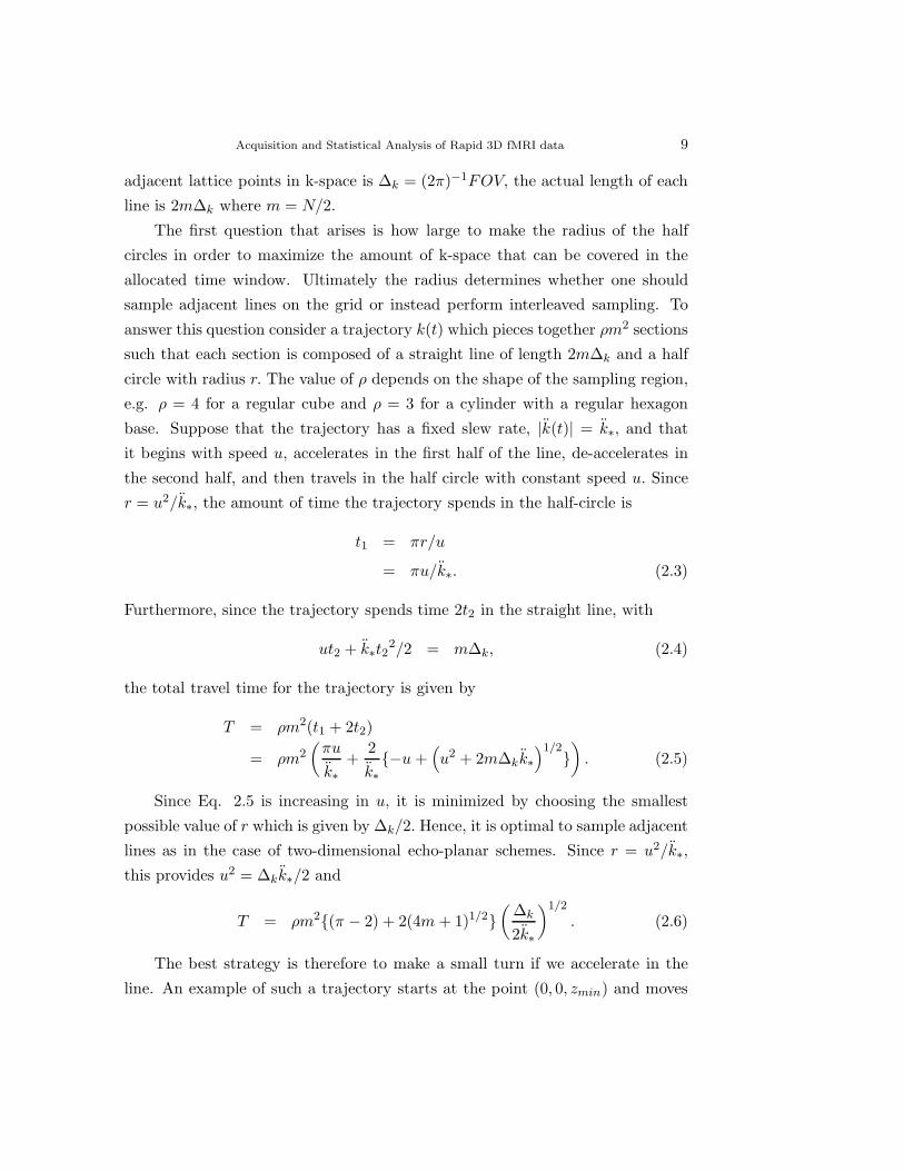
The best strategy is therefore to make a small turn if we accelerate in the

line. An example of such a trajectory starts at the point (0, 0, zmin) and moves


along the z-axis to the point (0, 0, zmax). Upon reaching this point the trajectory

makes a half circular loop over to the point (1, 0, zmax) and then continues along

the z-axis in the opposite direction until it reaches (1, 0, zmin). The trajectory

continues in a similar manner until it has completed a square spiral in the xy-

plane (Fig. 2.1A and B). Using this approach it is possible to sample the central

portion of 3D k-space with dimensions 14×14×14 in the allocated time window.

Further information about the practical implementation of the trajectory is left

for a companion paper to be submitted to an MRI journal.

−8 −6 −4 −2 0 2 4 6 8−8

−6

−4

−2

0

2

4

6

8

−5

0

5

−5

0

5

−5

0

5

A B

Figure 2.1: (A) An implementation of the echo-volumar imaging trajectory (B) Theecho-volumar imaging trajectory shown in (A) projected onto the xy-plane.

2.2. Reconstruction of EVI data

Once the central portion of 3D k-space has been collected, it needs to be

transformed into image-space for statistical analysis. A standard approach to-

wards reconstructing non-uniformly sampled k-space data is to interpolate the

data onto a Cartesian grid (Jackson, Meyer, Nishimura and Macovski (1991))

and thereafter apply the fast Fourier transform (FFT). Our data is sampled on

a Cartesian grid in the xy-plane, and it is relatively straightforward to use linear

interpolation to get uniformly spaced measurements in the z-direction as well. Af-

ter interpolation, our k-space data consists of 2, 744 (e.g. 14×14×14) uniformly

sampled measurements in 3D k-space. As the data is sampled on a grid, recon-


struction is straightforward using the FFT. The data is zero-filled to a resolution

of 64 × 64 × 64 prior to reconstruction, and a prolate spheroidal wave function

filter (PSWF) (Shepp and Zhang (2000); Yang, Lindquist, Shepp, Zhang, Wang

and Smith (2002); Lindquist (2003); Lindquist, Zhang, Glover, Shepp and Yang

(2006)) is applied to reduce truncation artifacts.

The PSWF is defined as the function with support on a finite sub-region of

k-space, whose inverse Fourier transform is maximally concentrated on a finite

region of image-space, B. Using the PSWF filter allows us to take the existing k-

space data and reconstruct an image with a point spread function determined by

the shape and size of the region B. The amount of k-space sampled will determine

how small we can make the region B and still obtain an efficient reconstruction

with minimal Gibbs artifacts. Ultimately, the diameter of B will have a reciprocal

relationship with the amount of k-space that is sampled (Lindquist and Wager

(2007)). Using this particular filter ties the reconstruction procedure together

with the spatial smoothing procedure. Ultimately, the spatial resolution using

our approach is equivalent to that obtained after applying a Gaussian filter with

FWHM of 12 mm to an image with dimensions 64×64×64 and a FOV of 20 cm.

It should be noted that spatial smoothing is almost always performed prior to

statistical analysis in fMRI using Gaussian filters with FWHM between 4−12 mm

(Smith (2003)). Hence, while our method provides images on the low end of this

spectrum, it is still on a comparable spatial resolution. However, it is important

to remember that our images are obtained twenty times faster than the standard

approach towards acquiring 3D fMRI data. In the Discussion we will discuss ways

to further increase the spatial resolution of our data using multi-coil techniques.

This is a major focus of future work.

2.3. Statistical Analysis

After reconstruction, the statistical analysis of the image space data is con-

ducted voxel-wise using a two step procedure. In the first step we detect re-

gions in the brain where there is a significant positive BOLD signal. These are

the regions that would typically be categorized as having task-induced neuronal

stimulation in a standard fMRI analysis. We will ultimately be more concerned

with detecting regions with significant negative BOLD signal. However, we feel it

is a natural assumption that regions having a significant dip will also ultimately


have a positive rise in BOLD signal if they are involved in the task at hand.

This step therefore works as a simple screening process to remove uninteresting

voxels, where there are no signs of task-induced activation, and allows for closer

and more data-intensive inspection of voxels that are actually involved in the

task. In the second step of the analysis we calculate the bootstrap distributions

for the amplitude of the negative dip, as well as for the time when the negative

dip reaches its peak (time-to-dip). Using these distributions we can perform sta-

tistical tests to determine whether there is a significant negative dip in a voxel,

as well as compare the relative timing of the dips across various regions of the

brain.

This second step is important as there is evidence that the negative dip

is more localized to areas of neural activity (Yacoub, Shmuel, Pfeuffer, Van De

Moortele, Adriany, Ugurbil and Hu (2001); Duong, Kim, Ugurbil and Kim (2000);

Kim, Duong and Kim (2000); Thompson, Peterson and Freeman (2004)) than

the subsequent rise which appears less spatially specific. Hence, we may be able

to prune away voxels that are simply adjacent to regions involved in the neuronal

activity, rather than being directly involved. In addition, since the negative dip

occurs in a time scale closer to that of the neural activity, there would appear to

be less confounding factors influencing the order of the time-to-dip in comparison

to traditionally used metrics such as the time-to-peak positive rise. Below follows

a more detailed outline of our two-step analysis:

Step One: After reconstructing the data into image-space we are left with a

sequence of T three-dimensional images, each of size 64× 64× 64. We model the

fMRI time course using a classical decomposition model. The fMRI signal from

voxel i, i = 1, · · · 643 can be modeled as:

Yi(t) = μi(t) + si(t) + zi(t) + εi(t). (2.7)

Here μi(t) is a drift term which we model using a quadratic polynomial function

μi(t) = β0 + β1t + β2t2. (2.8)

The term si(t) is a seasonal component that is due to heart rate and respi-

ration. There are a number of possible ways to model this, but we use a finite

impulse response (FIR) basis set which contains one free parameter for every


time point of the response we seek to model. A FIR basis set is able to capture

a response with arbitrary shape up to a given frequency limit determined by the

periodicity of the seasonal component. Including this term adds d parameters to

the model, where d is the periodicity of the seasonal component (in units of 0.1

s). We write this term as:

si(t) =d∑

j=1

γj(t)Ij(t) (2.9)

where

Ij(t) =

⎧⎨⎩

1 if j = (t mod d)

0 otherwise(2.10)

The term zi(t) represents the BOLD response to the neuronal stimuli and

it is the signal we are actually interested in studying. The shape of the BOLD

response depends on the experimental condition, and can be modeled using a

linear time-invariant system, where the stimulus function is the input and the

hemodynamic response is the impulse response function, i.e.

zi(t) = α∞∑

u=1

h(u)v(t − u). (2.11)

Here α is an unknown scalar, h(t) is the HRF and v(t) is the known stimulus

function which takes a value of 1 at time t if a stimulus is present and 0 otherwise.

If the HRF is assumed to take a particular known shape, this model can be

solved using the General Linear Model (GLM) framework (Worsley and Friston

(1995)), which is the standard approach towards fMRI data analysis. In this

work, we use the canonical HRF (e.g. SPMs double gamma function). To in-

crease its flexibility to handle slight temporal shifts in the onset of activation,

we also include a term for the temporal derivative (Friston, Josephs, Rees and

Turner (1998); Henson, Price, Rugg, Turner and Friston (2002)). This neces-

sitates adding an additional parameter corresponding to the convolution of the

stimulus function with the first derivative of the canonical HRF.

Finally, εi(t) is the noise present in the MR signal. Typically in fMRI this

is modeled either as an AR(p) or ARMA(1,1) process (Bullmore, Brammer,

Williams, Rabe-Hesketh, Janot, David, Mellers, Howard and Sham (1996); Pur-

don, Solo, Weissko and Brown (2001)). In this work we use an AR(2) process,


which adds three additional terms to our model. In summary our model can be

formulated as follows:

Yi(t) =2∑

j=0

βjtj +

d∑j=1

γj(t)Ij(t) (2.12)

+α1

∞∑u=1

h(u)v(t − u) + α2

∞∑u=1

h(u)v(t − u) + εi(t).

This model has a total of d + 5 regression parameters and 3 variance component

parameters.

For each voxel, the model is fit using an iterative generalized least-squares

approach, where the variance components and regression coefficients are alterna-

tively calculated and updated. Thereafter, t-statistics corresponding to the HRF

regressors are calculated, and statistical maps of the voxel-wise t-statistics are

constructed. The maps are thresholded and corrected for multiple comparisons

using the false detection rate (FDR) procedure (Benjamini and Hochberg (1995);

Genovese, Lazar and Nichols (2002)). This allows us to determine regions with

statistically significant signal corresponding to the positive BOLD signal.

Step Two: The time courses from each of the voxels deemed active in Step One

are extracted and analyzed further. They are decomposed into signal, trend and

seasonality components (see Fig 2.2), and the seasonal and trend components

are removed from the time course. The remaining time series is averaged over

the m repetitions of the stimuli to obtain estimates of the HRF. Note, that this

approach is only feasible if the time between repetitions is as long, or longer,

than the length of the HRF (e.g. 20s). Using the estimated HRF from each

voxel we can calculate the maximum amplitude of the positive rise, the minimum

amplitude of the negative dip, as well as the time-to-peak for both the rise and

dip.

Thereafter, for each time series, a statistical test based on the bootstrap

method (Efron and Tibshirani (1998)) was performed to test whether the dips

were statistically significant. Using resampling methods a bootstrap distribution

is calculated for both the peak amplitude of the negative BOLD response and the

time-to-dip. This is done by taking a sample of size m with replacement from the

m repetitions of the stimuli to create a new time course of the same length as the


0 500 1000 1500 2000 25000.84

0.86

0.88

0 500 1000 1500 2000 2500

0.83

0.84

0 500 1000 1500 2000 25000.027

0.028

0.029

0 500 1000 1500 2000 2500−0.02

0

0.02

Time (seconds)

A

B

C

D

Figure 2.2: (A) A typical time course decomposed into (B) quadratic drift, (C) periodicnuisance parameters and (D) fMRI signal. The length of the period for the nuisanceparameters is approximately 3 seconds and represents artifacts due to respiration.

original. The time course is averaged over the m repetitions, and the amplitude

and time-to-peak is recorded in a similar manner as for the original time series.

This procedure is repeated 2000 times to create a bootstrap distribution for

the amplitude, as well as the time-to-dip. Using the bootstrap distribution for

amplitude, tests were performed to determine whether the amplitude of the dips

were significantly different from zero.

Finally, for voxels with significant dips, a bootstrap distribution for the pair-

wise difference in time-to-dip was performed to determine whether the time-to-

dip was significantly different between voxels across the brain. This allowed us

to determine the order in which the dip occurs in various regions associated with

the task.

3. Experimental Design

Both the Cubic EVI trajectory and the reconstruction algorithm were imple-

mented in Matlab (Mathworks Inc.). To demonstrate the methods utility for dy-

namic studies, two high temporal resolution fMRI experiments were designed to

track the hemodynamic signals in the brain while the subject undergoes a visual-


motor activation paradigm and an auditory-motor-visual activation paradigm.

The first activation paradigm consisted of fifteen cycles of 20 s intervals.

At the beginning of each interval a 100 ms light flash was presented. The sub-

ject was instructed to press a button with their right thumb immediately after

sensing the flash, thereby leading to activation of the motor cortex. During the

20 second interval, images were acquired rapidly every 100 ms using our cubic

EVI trajectory. The sequence was repeated fifteen times, each time producing a

dynamic data set of 200 temporal points.

The second activation paradigm also consisted of fifteen cycles of 20 s inter-

vals. At the beginning of each interval a tone was sounded through headphones

which the subject was wearing. The subject was instructed to press a button with

their right thumb immediately after hearing the tone. Upon pressing the button

a 100 ms light flash was presented, leading to activation of the visual cortex.

During the 20 second interval, images were acquired rapidly every 100 ms using

our cubic EVI trajectory. The sequence was repeated fifteen times, each time

producing a dynamic data set of 200 temporal points. Reaction time data was

collected which measured the time between the onset of the tone and the button

press. As the flash appears exactly 30 ms after the button press, the reaction

time gives a measure of the timing of the appearance of the visual stimuli. This

information was compared to the timing of the dip in the visual cortex for each

cycle.

A healthy male volunteer participated in the study after giving informed

consent in accordance with a protocol approved by the Stanford Institutional

Review Board. In both experiments the first cycle was thrown out and the

resulting data consisted of 14 cycles with a total of 2800 time units. The resulting

k-space data was reconstructed and statistical analysis was performed as outlined

in the previous section. The data was acquired with an effective TE 30 ms, flip

angle 20 degrees, field of view 200 × 200 mm2, slice thickness 185 mm and

bandwidth 125 kHz. The experiment was performed on a 3.0 T whole body

scanner (GE magnet, General Electric Medical Systems, Milwaukee, WI, USA).

T2-weighted FSE scans were obtained for anatomic reference (TR/TE/ETL =

3000 ms/68 ms/12, 5 mm interleaved contiguous slices, FOV = 24 cm, 256×128

matrix).


4. Results

The feasibility of our rapid 3D imaging approach was tested experimentally

using a visual-motor and an auditory-motor-visual stimulation paradigm, both

described in the previous section. After data collection, the raw k-space data was

reconstructed into images of size 64×64×64, and the time courses corresponding

to the 643 voxels were analyzed for activation.

3.5

4.0

4.5

5.0

5.5

6.0

0.5

1.0

1.5

2.0

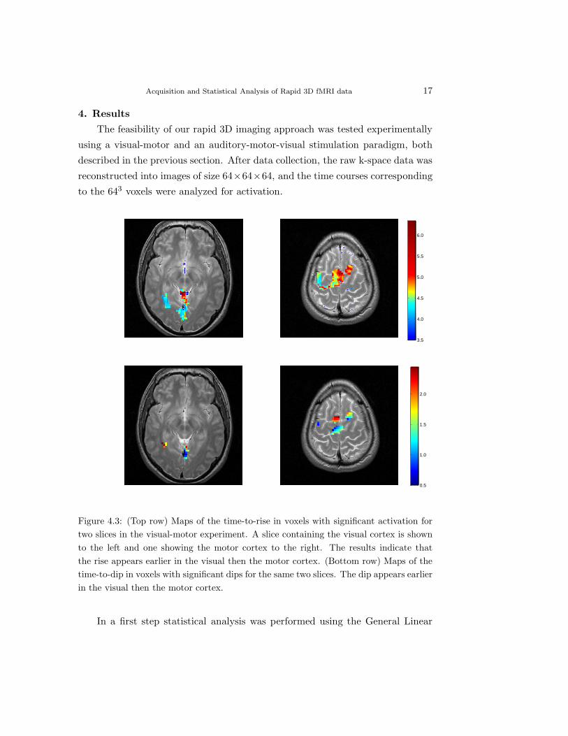
Figure 4.3: (Top row) Maps of the time-to-rise in voxels with significant activation fortwo slices in the visual-motor experiment. A slice containing the visual cortex is shownto the left and one showing the motor cortex to the right. The results indicate thatthe rise appears earlier in the visual then the motor cortex. (Bottom row) Maps of thetime-to-dip in voxels with significant dips for the same two slices. The dip appears earlierin the visual then the motor cortex.

In a first step statistical analysis was performed using the General Linear


Model (GLM) approach. The design matrix consisted of three columns corre-

sponding to a quadratic trend model for the signal drift, as well as, d columns

corresponding to the periodicity of the seasonal component. As the respiration is

the dominant source of seasonality in the data we used its periodicity, which was

empirically determined to be 3 seconds (i.e. d = 30), to determine the number

of parameters. In addition, two extra parameters corresponding to the canonical

HRF and its temporal derivative were added, giving a design matrix consisting

of a total of 35 columns. The top row of Fig 4.3 shows examples of statistical

parametric maps for two slices of the brain indicating voxels with significant task-

related activity (i.e. positive BOLD response) using a t-test (p − value ≤ 0.01).

A clear activation pattern is present both in the visual and motor cortices as

would be expected. For voxels that were deemed active in the GLM analysis,

their respective time courses were analyzed further. Each time course was decom-

posed into a trend component, a signal component and a seasonal component.

Fig. 2.2 shows the results of the decomposition of a representative time course.

The quadratic trend and the seasonal component were removed from each time

course and only the signal component is brought forth to the next stage of the

analysis.

For each voxel deemed to have a significant rise according to the GLM anal-

ysis, the time-to-rise was estimated. Results for two slices, one centered in the

visual and the other in the motor cortex, are shown in the top row of Fig. 4.3.

It is clear that the time-to-rise appears in the visual cortex prior to the motor

cortex. Among active voxels, a statistical test based on the use of the bootstrap,

was performed to test for significant dips (p − value < 0.05). The time-to-dip

was estimated for active voxels and the results for the same two slices are shown

in the bottom row of Fig. 4.3. Again it is clear that the activation seems to be

occurring in the visual cortex prior to that in the motor cortex.

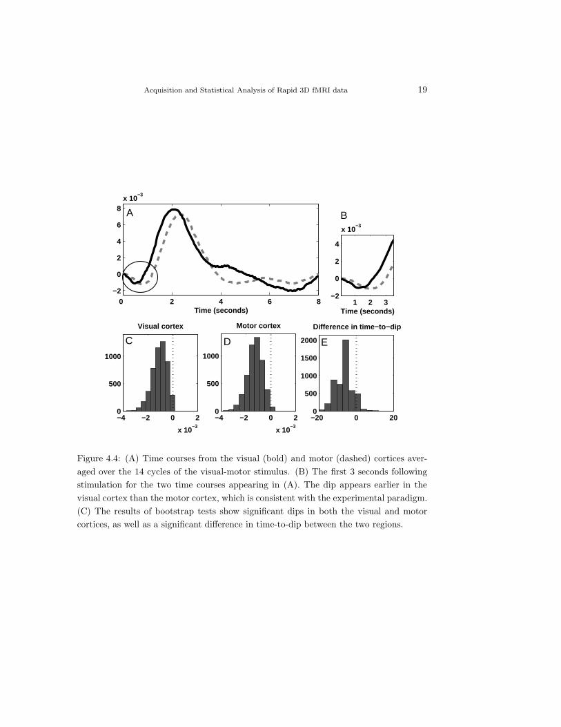
Fig. 4.4A shows the averages for two time courses extracted from the center

of the visual and motor cortices, respectively. We clearly see that the HRF

estimated from the visual cortex proceeds the one estimated from the motor

cortex throughout the course of the 20 second run. Fig. 4.4B shows a close-up of

the first 3 seconds following activation. A negative dip appears first in the visual

cortex, as makes sense since the visual cortex is logically the first region of the


0 2 4 6 8−2

0

2

4

6

8x 10

−3

Time (seconds)1 2 3

−2

0

2

4

x 10−3

Time (seconds)

−4 −2 0 2

x 10−3

0

500

1000

Visual cortex

−4 −2 0 2

x 10−3

0

500

1000

Motor cortex

−20 0 200

500

1000

1500

2000

Difference in time−to−dip

A B

C D E

Figure 4.4: (A) Time courses from the visual (bold) and motor (dashed) cortices aver-aged over the 14 cycles of the visual-motor stimulus. (B) The first 3 seconds followingstimulation for the two time courses appearing in (A). The dip appears earlier in thevisual cortex than the motor cortex, which is consistent with the experimental paradigm.(C) The results of bootstrap tests show significant dips in both the visual and motorcortices, as well as a significant difference in time-to-dip between the two regions.


brain that begins to work on the image. After a few hundred milliseconds delay

we see a delayed negative response in the motor cortex. Bootstrap tests (Fig.

4.4C) confirm these results, and show that while both dips are significant, the dip

in the visual cortex occurs at a significantly earlier time point compared to that

of the motor cortex. In this experiment both the timing of the dip and rise give

compelling evidence that neuronal activity is taking place in the visual cortex

prior to the motor cortex as would be expected by the experimental paradigm.

3.5

4.0

4.5

5.0

5.5

6.0

6.5

0.5

1.0

1.5

2.0

Figure 4.5: (Top row) Maps of the time-to-rise in voxels with significant activation fortwo slices in the auditory-motor-visual experiment. The slices that are included coverthe visual (left) and motor cortices (right). (Bottom row) Maps of the time-to-dip invoxels with significant dips for the same two slices.

The exact same statistical analysis was repeated for the auditory-motor-


visual stimulation paradigm. For each voxel deemed to have a significant rise

according to the GLM analysis, the time-to-peak was estimated. Results for two

slices, centered in the visual and motor cortices, respectively, are shown in the

top row of Fig. 4.5. It is important to note that in this experiment the order

of activation should now be auditory, followed by motor, followed by visual.

While, the signal in the auditory does appear to peak first, there appears to be

confounding in the timing of the peaks in the visual and motor cortices. This can

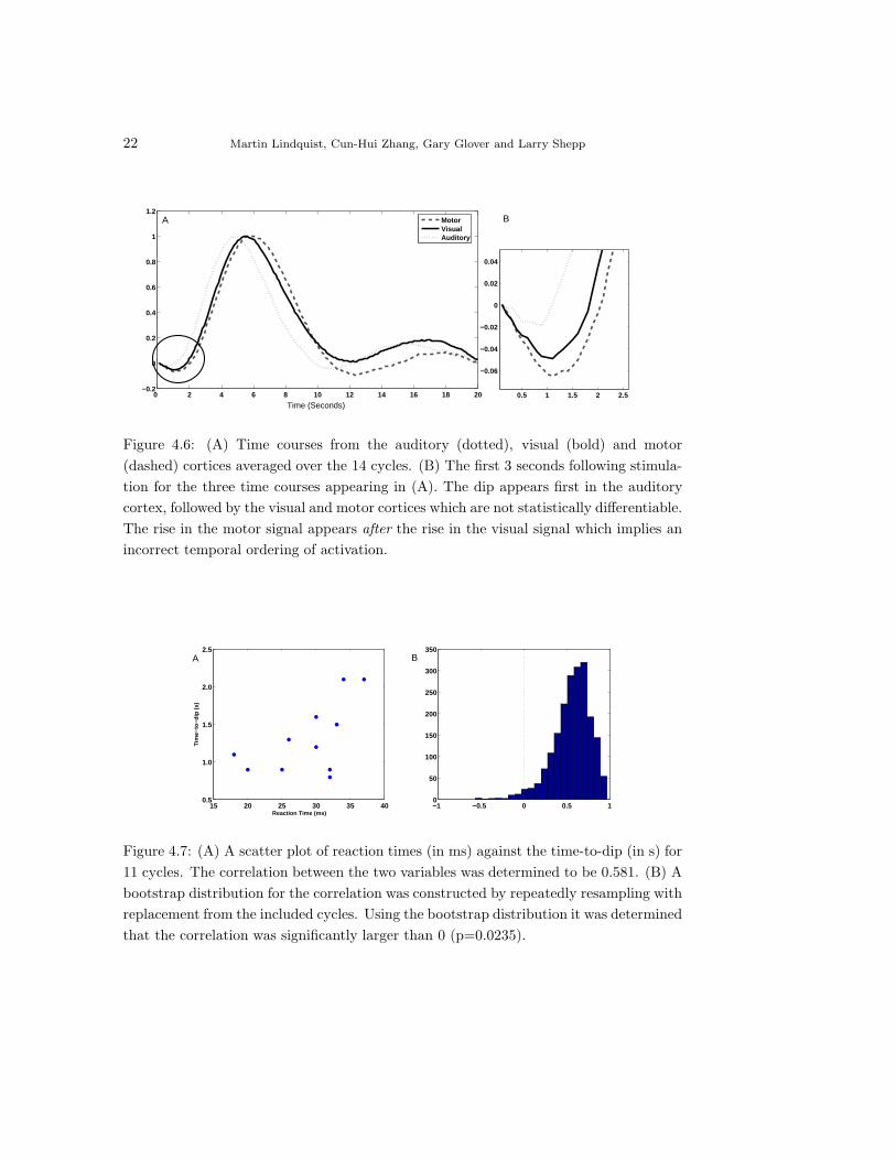
be further seen in Fig. 4.6A where clearly the signal over the motor cortex peaks

after the visual cortex. However, studying the dip alleviates this confounding,

which can be seen in both Figs. 4.5 and 4.6B. The difference in the time-to-

dip between the visual and motor cortices is not statistically different from zero.

However, this is hardly surprising as the time between button press and visual

stimuli is only 30 ms. A follow-up experiment should be performed to study how

far apart these stimuli must lie in order for one to be able to discriminate between

them. Included in Fig. 4.6 is also the signal over the auditory cortex whose dip

and rise both peak prior to that of the visual and motor cortices. This is to

be expected as the tone is presented before the button is pressed and the visual

stimulus is presented.

Finally, the time-to-dip in the visual cortex was manually read off for each

individual cycle and compared to the corresponding reaction time data. The

reaction time data gives a measure of the shift in the onset of the visual stimulus

in each cycle. Cycles whose reaction times were outliers in the range of common

reaction times were removed from the analysis, due to the influence they would

have on the resulting correlation. Additionally, cycles without a clear dip were

removed. Fig. 4.7A shows a scatter plot of reaction time (in ms) against the

time-to-dip (in s) for the 11 cycles that remained. The correlation between the

two variables was 0.581. The relatively strong correlation indicates that the dip

appears to be providing information about the onset of the underlying visual

stimulus. A bootstrap distribution for the correlation was constructed by resam-

pling with replacement 2000 times from the 11 cycles. Using this distribution we

were able to perform a significance test that indicated that the correlation was

significantly larger than 0 (p − value = 0.0235). The bootstrap distribution is

shown in Fig. 4.7B.


0 2 4 6 8 10 12 14 16 18 20−0.2

0

0.2

0.4

0.6

0.8

1

1.2

Time (Seconds)0.5 1 1.5 2 2.5

−0.06

−0.04

−0.02

0

0.02

0.04

MotorVisualAuditory

A B

Figure 4.6: (A) Time courses from the auditory (dotted), visual (bold) and motor(dashed) cortices averaged over the 14 cycles. (B) The first 3 seconds following stimula-tion for the three time courses appearing in (A). The dip appears first in the auditorycortex, followed by the visual and motor cortices which are not statistically differentiable.The rise in the motor signal appears after the rise in the visual signal which implies anincorrect temporal ordering of activation.

15 20 25 30 35 400.5

1.0

1.5

2.0

2.5

Reaction Time (ms)

Tim

e−to

−dip

(s)

−1 −0.5 0 0.5 10

50

100

150

200

250

300

350A B

Figure 4.7: (A) A scatter plot of reaction times (in ms) against the time-to-dip (in s) for11 cycles. The correlation between the two variables was determined to be 0.581. (B) Abootstrap distribution for the correlation was constructed by repeatedly resampling withreplacement from the included cycles. Using the bootstrap distribution it was determinedthat the correlation was significantly larger than 0 (p=0.0235).


To summarize the results of the experiments, we have shown reproducibly

that significant dips are present in both the visual and motor cortices. In addi-

tion, there is a statistically significant difference in the time-to-dip between the

visual and motor cortices in our first experiment, which is consistent with the

experimental paradigm. In the second experiment there is also a significant dip

in the auditory cortex (again consistent with the paradigm) followed by dips in

the visual and motor cortices which are not statistically differentiable. However,

if we instead use the time-to-peak rise as a metric, the order of activation between

the visual and motor cortices is confounded. This strengthens our notion that

studying the initial negative BOLD response is a crucial tool for determining the

timing of activation in the brain.

5. Discussion

This paper introduces a novel approach towards the acquisition and statisti-

cal analysis of rapid 3D fMRI data. There are a number of benefits to performing

rapid imaging studies. First, it may allow one to study the initial negative BOLD

response, instead of solely depending on the positive BOLD signal, for purposes

of determining active regions as well as the order of activation in multiple active

regions. Secondly, it allows for the efficient removal of physiological noise due to

cardiac and respiratory effects. In a typical fMRI analysis, the time resolution is

on the order of 2 seconds. Since respiration gives rise to a periodic function, with

a period length of approximately 3 seconds, the Nyquist criteria does not allow

us to fully reconstruct this signal. Rapid fMRI (with a temporal resolution on

the order of 100 ms) circumvents this issue and allows for efficient reconstruction

of the underlying signal without the problem of aliasing. This is beneficial as it

allows us to significantly clean up the fMRI signal prior to analysis and obtain

more accurate estimates of the hemodynamic response function. Finally, rapid

imaging alleviates issues related to the fact that spatially separate regions of the

brain are sampled at different times, thus negating the need for slice-time cor-

rection. In addition, it may also allow for more accurate correction of subject

motion, as movement occurring during the acquisition of each individual volume

will be reduced.

While the existence of the negative response remains controversial and has

caused a great deal of debate, the idea of being able to systematically detect


and perform inference about an early response to neuronal activity is appealing.

While the results presented in this work are based on a single subject, they are

done on different days and our statistical analyses confirm the negative dip based

on all individual data sets. However, the experiments will ultimately need to be

repeated on a larger group of subjects to gain more conclusive evidence of the

existence of the initial negative response. The current work may therefore be seen

as more of a proof of concept of our imaging and analysis procedure, rather than a

proof of our ability to reliably and reproducibly detect the initial negative BOLD

signal in a population of subjects. Further experiments need to be performed to

determine (i) whether the dip can be reliably detected over multiple subjects,

and (ii) whether in these subjects it provides an accurate picture of the timing of

activation. However, we feel that if these results were to hold up, the technique

would be an extremely valuable tool in neuroimaging studies.

In the data sets that are presented in this paper, we have shown reproducibly

that significant dips are present in both the visual and motor cortices. In addi-

tion, there is a statistically significant difference in the time-to-dip between the

visual and motor cortices in our first experiment, which is consistent with the

experimental paradigm. In the second experiment there is also a significant dip

in the auditory cortex (again consistent with the paradigm) followed by dips in

the visual and motor cortices which are not statistically differentiable. However,

if we instead use the time-to-peak rise as a metric, the order of activation be-

tween the visual and motor cortices is confounded. Our results indicate that the

negative response may contain valuable information regarding the timing of ac-

tivation, information that may be confounded when studying the positive BOLD

response. This strengthens our notion that studying the initial negative BOLD

response can be an important tool for determining the exact timing of activation

in the brain.

It should be noted that in both experiments we performed there appears

to be an increase in the number of false negatives when looking for voxels with

significant dips compared to rise. This is made clear by comparing the two rows

in Figs. 4.3 and 4.5. The reason for this discrepancy may be due to the fact

that the signal-to-noise ratio for the rise is on the order of 5 times larger than

that of the dip. Alternatively, there is evidence that the initial negative BOLD


response is more localized to areas of neural activity (Yacoub, Le and Hu (1998);

Duong, Kim, Ugurbil and Kim (2000); Kim, Duong and Kim (2000); Thompson,

Peterson and Freeman (2004)) than the subsequent rise. Hence, the decreased

number of active voxels may in fact be giving a more accurate picture of the true

activation patterns in the brain. However, this statement is hard to verify, in

part because the low spatial resolution provided by the current implementation

of the method, and the fact that we have sacrificed spatial resolution to obtain

our increase in temporal resolution proves to be somewhat of a liability in this

respect. However, advances in multi-coil techniques (Sodickson and Manning

(1997); Pruessmann, Weiger, Scheidegger and Boesiger (1999)) give an avenue to

bridge this gap in the future. In these techniques, multiple k-space measurements

can simultaneously be made and prior knowledge about RF field distributions

or the image sensitivity of the coils can be utilized to construct images from

under-sampled k-space data. We have recently implemented two new trajectories

that allow us to obtain images with a temporal resolution of 100 ms a spatial

resolution on the order of 25 × 25 × 17 and 46 × 46 × 17, respectively. With the

latter spatial resolution we are quickly approaching the resolution that is used

in standard fMRI experiments. However, the temporal resolution is increased

10-fold. These new trajectories constitute a second step in our rapid imaging

method, and the results of these trajectories will be presented in future work.

6. Conclusions

A new approach towards rapid fMRI is introduced where a small central re-

gion of 3D k-space is sampled every 100 ms and a low spatial resolution snapshot

of the brain with extremely high temporal resolution is obtained. In addition we

introduce a new approach towards the statistical analysis of the resulting high-

frequency fMRI data. The feasibility and efficiency of the combined acquisition

and analysis approach is confirmed using data both from a visual-motor task

and an auditory-motor-visual task. The increased temporal resolution allows us

for the first time to perform a statistical analysis over the brain based solely

on the initial negative BOLD response, rather than the sluggish positive BOLD

response. In the visual-motor experiment there are coherent regions in both the

visual and motor cortices with a significant initial negative BOLD signal. Fur-

ther, the time to the peak negative response is shown to be significantly earlier


in the visual cortex which is consistent with the experimental paradigm. In the

auditory-motor-visual experiment there is a significant dip in the auditory cortex

followed by dips in the visual and motor cortices which are not statistically dif-

ferentiable. However, if we instead use the time-to-peak positive BOLD response

as a metric, the order of activation between the visual and motor cortices are

confounded. This leads us to believe that studying the initial negative BOLD

response can be an important tool for determining the timing of activation across

different regions of the brain, though further experiments need to be performed

to verify its reproducibility.

References

Benjamini, Y. and Hochberg, Y. (1995). Controlling the False Discovery Rate:

A Practical and Powerful Approach to Multiple Testing. Journal of the

Royal Statistical Society, Series B. 57:289-300.

Bullmore, E.T., Brammer, M.J., Williams, S.C.R., Rabe-Hesketh, S., Janot,

N., David, A.S., Mellers, J.D.C., Howard, R. and Sham, P. (1996). Statisti-

cal methods of estimation and inference for functional MR image analysis.

Magnetic Resonance in Medicine 35, 261-277.

Buxton, R. and Frank, L. (1997). A model for the coupling between cerebral

blood flow and oxygen metabolism during neural stimulation. J. Cereb.

Blood Flow Metab. 17(1), 64-72.

Cho, Z.H., Ro, Y.M. and Lim, T.H. (1992). NMR venography using the suscepti-

bility effect produced by deoxyhemoglobin. Magnetic Resonace in Medicine

28 25-38.

Duong, T.Q., Kim, D.S., Ugurbil, K. and Kim, S.G. (2000). Spatio-temporal

dynamics of the BOLD fMRI signals: Toward mapping columnar structures

using the early negative response. Magnetic Resonance in Medicine 44,

231-242.

Efron, B. and Tibshirani, R.J. (1998). An Introduction to the Bootstrap, Chap-

man & Hall/CRC.


Ernst, T. and Hennig, J. (1994). Observation of a fast response in functional

MR. Magnetic Resonance in Medicine 32, 146-149.

Friston, K.J., Josephs, O., Rees, G. and Turner, R. (1998). Nonlinear event-

related responses in fMRI. Magnetic Resonance in Medicine 39(1), 41-52.

Friston, K.J., Penny, W., Phillips, C., Kiebel, S., Hinton, G., and Ashburner, J.

(2002). Classical and Bayesian Inference in Neuroimaging: Theory. Neu-

roImage 16, 465-483.

Gao, J.H., Xiong, J., Lai, S., Haacke, E.M., Woldorff, M.G., Li, J. and Fox,

P.T. (1996). Improving the Temporal Resolution of Functional MR Imaging

Using Keyhole Techniques. Magnetic Resonance in Medicine 35, 854-860.

Genovese, C.R., Lazar, N.A. and Nichols, T.E. (2002). Thresholding of Sta-

tistical Maps in Functional Neuroimaging Using the False Discovery Rate.

NeuroImage 15:870-878.

Haacke, E.M., Brown, R.W., Thompson, M.R. and Venkatesan, R. (1999). Mag-

netic Resonance Imaging: Physical Principles and Sequence Design. John

Wiley & Sons, Inc.

Harvey, P.R. and Mansfield, P. (1996). Echo-volumar imaging (EVI) at 0.5 T:

First Whole-Body Volunteer Studies. Magnetic Resonance in Medicine 35,

80-88.

Henson, R.N., Price, C.J., Rugg, M.D., Turner, R. and Friston, K.J. (2002).

Detecting latency differences in event-related BOLD responses: application

to words versus nonwords and initial versus repeated face presentations.

NeuroImage 15(1), 83-97.

Hu, X., Le, T.H. and Ugurbil, K. (1997). Evaluation of the early response

in fMRI in individual subjects using short stimulus duration. Magnetic

Resonance in Medicine 37, 877-884.

Irarrazabal, P. and Nishimura, D.G. (1995). Fast Three Dimensional Magnetic

Resonace Imaging. Magnetic Resonance in Medicine 33, 656-662.


Jackson, J, Meyer, C.H., Nishimura, D.G. and Macovski, A. (1991). Selec-

tion of a Convolution Function for Fourier Inversion Using Gridding, IEEE

Transactions on Medical Imaging 10, 1, 473478.

Kim, D.S., Duong, T.Q. and Kim, S.G. (2000). High-resolution mapping of

iso-orientation columns by fMRI. Nature Neuroscience 3(2), 164-169.

Liang, Z.P. and Lauterbur, P.C. (1994). An Efficient Method for Dynamic

Magnetic Resonance Imaging. IEEE Transactions on Medical Imaging 13,

677-686.

Lindquist, M.A. (2003). Optimal Data Acquisition in fMRI Using Prolate

Spheroidal Wave Functions. International Journal of Imaging Systems and

Technology 13, 803-812.

Lindquist, M.A., Zhang, C.H., Glover, G., Shepp, L.A. and Yang, Q.X. (2006).

A Generalization of the Two Dimensional Prolate Spheroidal Wave Func-

tion Method for Non-rectilinear MRI data Acquisition Methods. IEEE

Transactions in Image Processing 15(9), 2792-2804.

Lindquist, M.A. and Wager, T.D. (2007). Spatial Smoothing in fMRI using

Prolate Spheroidal Wave Functions. To appear in Human Brain Mapping.

Logothetis, N. (2000). Can current fMRI techniques reveal the micro-architecture

of cortex? Nature Neuroscience 3, 413.

Malonek, D. and Grinvald, A. (1996). The imaging spectroscopy reveals the

interaction between electrical activity and cortical microcirculation: impli-

cation for optical, PET and MR functional brain imaging. Science 272,

551-554.

Mansfield, P. (1977). Multi-planar image formation using NMR spin echoes.

Journal of Physics C10, L55-L58.

Mansfield, P., Howseman, A.M. and Ordidge, R.J. (1989). Volumar imaging

using NMR spin echos: echo-volumar imaging (EVI) at 0.1 T. Journal of

Physics E 22, 324-330.


Mansfield, P., Coxon, R. and Hykin, J. (1995). Echo-volumar imaging (EVI) at

3.0 T: First Normal Volunteer and Functional Imaging Results. Journal of

Computer Assisted Tomography 19(6), 847-852.

Menon, R.S., Ogawa, S., Hu, X., Strupp, J.S., Andersen, P. and Ugurbil, K.

(1995). Bold based functional MRI at 4 Tesla includes a capillary bed

contribution: echo-planar imaging mirrors previous optical imaging using

intrinsic signals. Magnetic Resonance in Medicine 33, 453-459.

Mir, R., Guesalaga, A., Spiniak, J., Guarini, M. and Irarrazaval, P. (2004). Fast

three-dimensional k-space trajectory design using missile guidance ideas.

Magnetic Resonance in Medicine 52(2), 329-36.

Ogawa, S., Tank, D.W., Menon, R., Ellerman, J.M., Kim, S.G., Merkle, H. and

Ugurbil, K. (1992). Intrinsic signal changes accompanying sensory simula-

tion: functional brain mapping and magnetic resonance imaging. Proceed-

ings of the National Academy of Sciences 89, 5951-5955.

Ogawa, S., Lee, T.M. and Barrere, B. (1993). The sensitivity of magnetic

resonance image signals of a rat brain to changes in the cerebralvenous

blood oxygenation. Magnetic Resonance in Medicine 29, 205-210.

Ogawa, S., Menon, R., Tank, D.W., Kim, S.G., Merkle, H., Ellerman, J.M. and

Ugurbil, K. (1993). Functional brain mapping by blood oxygenation level-

dependent contrast magnetic resonance imaging: A comparison of signal

characteristics with a biophysical model. Biophysical Journal, 64, 803-812.

Panych, L.P., Oesterle, C., Zientara, G.P. and Hennig, J. (1996). Implementa-

tion of a Fast Gradient-Echo SVD Encoding Technique for Dynamic Imag-

ing. Magnetic Resonance in Medicine 35, 554-562.

Pruessmann, K.P., Weiger, M., Scheidegger, M.B. and Boesiger, P. (1999).

SENSE: sensitivity encoding for fast MRI. Magnetic Resonance in Medicine

42(5):952-956.

Purdon, P.L., Solo, V., Weissko, R.M. and Brown, E. (2001). Locally regular-

ized spatiotemporal modeling and model comparison for functional MRI.

NeuroImage 14, 912-923.


Sabat, S., Mir, R., Guarini, M., Guesalaga, A. and Irarrazaval, P. (2003). Three

dimensional k-space trajectory design using genetic algorithms. Magnetic

Resonance Imaging 21(7), 755-64.

Shepp, L.A. and Zhang, C.-H. (2000). Fast Functional Magnetic Resonance

Imaging via Prolate Wavelets. Applied and Computational Harmonic Anal-

ysis 9, 99-119.

Smith, S.M. (2003). Preparing fMRI data for statistical analysis. In: Jezzard,

P., Matthews, P. M., Smith, S. M. (Eds.), Functional MRI: an introduction

to methods, Oxford University Press, Oxford, UK.

Sodickson, D.K. and Manning, W.J. (1997). Simultaneous acquisition of spatial

harmonics (SMASH): fast imaging with radiofrequency coil arrays. Mag-

netic Resonance in Medicine 38(4), 591-603.

Thompson, J.K., Peterson, M.R. and Freeman, R.D. (2004). High-resolution

neurometabolic coupling revealed by focal activation of visual neurons. Na-

ture Neuroscience 7, 919-920.

van Vaals, J.J., Brummer, M.E., Dixon, W.T., Tuithof, H.H., Engels, H., Nelson,

R.C., Gerety, B.M., Chezmar, J.L. and den Boer, J.A. (1993). Keyhole

Method for Accelerating Imaging of Contrast Agent Uptake. J. Magn.

Reson. Imaging 3, 671-675.

Worsley, K.J. and Friston, K.J. (1995). Analysis of fMRI Time-Series revisited

- Again. NeuroImage 2, 173-181.

Yacoub, E., Le, T.H. and Hu, X. (1998). Detecting the early response at 1.5

Tesla. NeuroImage 7, S266.

Yacoub, E., Shmuel, A., Pfeuffer, J., Van De Moortele, P.F., Adriany, G., Ugur-

bil, K. and Hu, X. (2001). Investigation of the initial dip in fMRI at 7 Tesla.

NMR in Biomedicine 14, 7-8, 408 - 412.

Yang, Q.X., Lindquist, M.A., Shepp, L.A., Zhang, C.H., Wang, J. and Smith,

M. (2002). The Two Dimensional Prolate Spheroidal Wave Function for

MRI. Journal of Magnetic Resonance 58, 43-51.


Zientara, G.P., Panych, L.P. and Jolesz, F.A. (1994). Dynamically Adaptive

MRI with Encoding by Singular Value Decomposition. Magnetic Resonance

in Medicine 32, 268-274.

Department of Statistics, Columbia University

E-mail: [email protected]



Department of Radiology, Stanford University




the acquisition and statistical analysis of rapid 3d fmri …martin/papers/ss_rfmri.pdf · the...

Documents