NASA-CR-194609

1_I i31

Research Institute for Advanced Computer ScienceNASA Ames Research Center

i7P

The Alignment-Distribution Graph

Siddhartha ChatterjeeJohn R. Gilbert

Robert Schreiber

(NASA-CR-194609) THE

ALIGNMENT-DISTRIBUTION GRAPH

(Research Inst. for Advanced

Computer Science) 17 p

N94-15956

Uncl as

0191131

RIACS Technical Report 93.06 August 1993

To appear in the Proceedings of the Sixth Annu'al Languages and Compilers for Parallelism Workshop,Portland, OR, 12-14 August 1993.

https://ntrs.nasa.gov/search.jsp?R=19940011483 2020-01-05T12:42:22+00:00Z

The Alignment-Distribution Graph

Siddhartha ChatterjeeJohn R. Gilbert

Robert Schreiber

The Research Institute for Advanced Computer Science is operated by Universities Space Research

Association, The American City Building, Suite 212, Columbia, MD 21044, (410) 730-2656

Work reported herein was supported by NASA via Contract NAS 2-13721 between NASA and the Universities

Space Research Association (USRA). Work was performed at the Research Institute for Advanced Computer

Science (RIACS), NASA Ames Research Center, Moffett Field, CA 94035-1000.

The Alignment-Distribution Graph

Siddhartha Chatterjee * John R. Gilbert t Robert Schreiber *

Abstract

Implementing a data-parallel language such as Formm 90 on a distn_outed-memory parallel computer requires

distn"outing aggregate data objects (such as arrays) among the memory modules attached to the processors. The

mapping of objects to the machine determines the amount of residual communication needed to bring operands

of parallel operations into alignment with each other. We present a program representation called the alignment-

distribution graph that makes these communication requirements expliciL We descn'be the details of the representation,show how to model communication cost in this framework, and outline several algorithms for determining object

mappings that approximately minimize residual communication.

1 Introduction

When a data-parallel language such as Fortran 90 is implemented on a distributed-memory parallel computer, the

aggregate data objects (arrays) have to be distributed among the multiple memory units of the machine. The mappingof objects to the machine determines the amount of residual communication needed to bring operands of parallel

operations into alignment with each other. A common approach is to break the mapping into two stages: first, analignment that maps all objects to an abstract Cartesian grid called a template, and then a distribution that maps thetemplate to the processors. This two-phase approach separates language issues from machine issues; it is used inFortran D [6], High Performance Fortran [8], and CM-Fortran [13].

A compiler for a data-parallel language attempts to produce data and work mappings that reduce completiontime. Completion time has two components: computation and communication. Communication can be separatedinto intrinsic and residual communication. Intrinsic communication arises from operations such as reductions that

must move data as an integral part of the operation. Residual communication arises from nonlocal data referencesin an operation whose operands are not mapped to the same processors. We use the term realignment to refer toresidual communication due to misalignment, and redistribution to refer to residual communication due to changes in

distribution.In this paper, we describe a representation of array-based data-parallel programs called the Alignment-Distribution

Graph, or ADG for short. We show how to model residual communication cost using the ADG, and discussalgorithms [2, 3, 4] for analyzing the alignment requirements of a program. The ADG is closely related to the staticsingle assignment (SSA) form of programs developed by Cytron et al. [5], but is tailored for alignment and distributionanalysis. In particular, it uses new techniques to represent the residual communication due to loop-carried dependences,assignment to sections of arrays, and transformational array operations such as reductions and spreads. The ADGprovides a detailed and realistic model of residual communication cost that accounts for a wide variety of programfeatures; it allows us to handle alignment and distribution as discrete optimization problems.

The remainder of the paper is organized as follows. Section 2 motivates and formally describes the AZX3representation of programs. Section 3 describes how the ADG is used to model the communication cost of a program.Section 4 discusses approximations that we make in the model presented in Section 2 for reasons of practicality.

"Research Institute for Advanced Computer Science, Mail Stop T045-1, NASA Ames Research Center, Motfett Field, CA 94035-1000

(sc_riaes.edu, schreib_riacsledu). "l]aework of these authors was supported by the NAS Systems Division via Contract NAS 2-13721 betweenNASA and the Universities Space Research Association (USRA).

! Xerox Palo Alto Research Center, 3333 Coyote IZaqlRoad, Palo Alto, CA 94304-1314 (g_ert@pare.xerox.eom). Copyright (_)1993 by Xerox

Coqx_tion. All rights n_aved.

Section5 outlinessome algorithmsforalignmentanalysisthatusetheADG. Our previouspapers[2,3,4]contain

moredetailsaboutthealgorithms.Section6comparesthe_ representationwithSSA formandwiththepreference

graph,anotherrepresentationusedinalignmentand distributionanalysis.Section7 discussesopenproblemsand

futurework.

2 The ADG representation of data.parallel programs

The ADG is a directed graph representation of data flow in a pmgrarn. Nodes in the ADG represent computation;

edgesrepresent flow of dataAlignments are associated with endpoints of edges, which we call ports. A node constrains the relative alignments

of the ports representing its operands and its results. Realignment occurs whenever the ports of an edge have differentalignments. The goal of alignment analysis is to determine alignments for the ports that satisfy the node constraintsand minimize the total realignment cost, which is a sum over edges of the cost of all realignment that occurs on that

edge during program execution.Similar mechanisms can be used for determining distributions. In the distribution analysis method that we foresee,

the template has a distribution at each node of the ADG; the alignment of an object to the template and the distributionof the template jointly define the distribution of the object onto processors at that node. The distributions are chosento minimize an execution time model that accounts for redistribution cost (again associated with edges of the ADG)

and computation cost, associated with nodes of the ADG and dependent on the distribution as well. For the remainder

of this paper, however, we focus on alignment analysis.The ADG distinguishes between prograrn arrayvariables and army-valued objects in order to separate names from

values. An array-valued object (object for short) is created by every array operation and by every assignment to asection of an array. Assignment to a whole array, on the other hand, names an object. The algorithms presented inSection 5 determine an alignment for each object in the program rather than for each program variable.

2.1 A summary of SSA form

A program is in SSAform if each variable is the target of exactly one assignment statement in the program text [5]. Anyprogram can be translated to SSA form by renaming variables and introducing a pseudo-assignment called a S-functionat some of the join nodes in the control flow graph of the program. Cytron et al. [5] present an efficient algorithmto compute minimal SSA form (i.e., SSA form with the smallest number of S-functions inserted) for programs witharbitrarycontrol flow graphs. Johnson and Pingali [9] have recently improved the complexity of SSA-conversion.

In common usage, SSA form is usually defined for sequential scalar languages, but this is not a fundamentallimitation. It can be used for array languages if care is taken to properly model references and updates to individual

array elements and array sections [5, §3.1]. The ADG uses SSA form in this manner.A major contribution of SSA form is the separation between the values manipulated by a program and the storage

locations where the values are kept. This separation, which allows greater opportunities for optimization, is the primaryreason for basing the ADG on SSA form. After optimization, the program must be translated from SSA form to object

code. Cytron et al. discuss two optimizations (dead code elimination and storage allocation by coloring) that produceefficient object code [5, §7].

2.2 Ports and alignment

The ADG hasaportfor._h textualdefinitionoruseofanobject.Portsarejoinedby edgesasdescribedbelow.The

portsthatrepresenttheinputsandoutputsofaprogramoperationaregroupedtogethertoformanode.Some portsare

named andcorrespondtoprogramvariables;othersareanonymousand correspondtointermediatevaluesproduced

by the computation ....................................................The principal attribute of a port is its alignment, which is a one-to-one mapping of the elements ofthe object into

the cells of a template, We use the notation

a(01,... ,0d)[][_l(01,...,od),-'',ff,(01,..-,0d)]

2

For_angO

real A(100,100), V(200)

do k - 1, 100

A(k,l:100) - A(k,l:100) + V(klk+99)

enddo

SSA form

_eal A1(100,100), A2(100,100), A3(100,100)

real V(200)

do k - 1, 100

A2 - pI_L(AI, A3)

A3 - UIxlate(A2, (k, lzl00),

A2(k,lzl00) + Vl(ksk+99))

enddo

Section

(k,l:lO0)

Fanout /

Vout

Section [ !(k:k+99) I1,/00 1

;_l,j +11

Branch J

¢Fallout 1

Figure 1: A Fortran 90 program fragment, its SSA form, and its ADG.

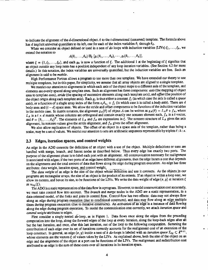
to indicate the alignment of the d-dimensional object A to the t-dimensional (unnamed) template. The formula abovehas d implicit universal quantifiers to its left, one for each of the index variables 01 through Od.

When we consider an object defined or used in a nest of do loops with induction variables (LIVs) _1,. •., _k, weextend the notation to

A(O_,..., Od) m_ _(0_,..., Sd), " ", g,(Ox,..., Od)],

where _ -- (1,_1,... ,_k), and each gk is now a function of _. The additional 1 at the beginning of_ signifies thatan object outside any loop nests has a position independent of any loop iteration variables. (See Section 4.2 for moredetails.) In this notation, the index variables are universally quantified, but the induction variables are free. Such an

alignment is said to be mobile.High Performance Fortran allows a program to use more than one template. We have extended our theory to use

multiple templates, but in this paper, for simplicity, we assume that all array objects are aligned to a single template.We restrict our attention to alignments in which each axis of the object maps to a different axis of the template, and

elements are evenly spaced along template axes. Such an alignment has three components: ax/s (the mapping of objectaxes to template axes), stride (the spacing of successive elements along each template axis), and offset (the position ofthe object origin along each template axis). Each 9j is thus either a constant fj (in which case the axis is called a spaceaz/s), or a function of a single array index of the form sj 0o, + fj (in which case it is called a body axis). There are d

body axes and (t - d) space axes. We allow the stride and offset components to be functions of the induction variablesin the mobile case. In matrix notation, the alignment gA(O) of object A can be written as 9A(0) = LaO + fA, where

La is a t x d matrix whose columns are orthogonal and contain exactly one nonzero element each, fa is a t-vector,and 0 = (01,..., 0a) r. The elements of La and fA are expressions in _. The nonzero structure of La gives the axisalignment, its nonzero values give the stride alignment, and fA gives the offset alignment.

We also allow replication of objects. The offset of an object in a space axis of the template, rather than being a

scalar, may be a set of values. We restrict our attention to sets are arithmetic sequences representable by triplets g: h : s.

2.3 Edges, iteration spaces, and control weights

An edge in the ADG connects the definition of an object with a use of the object. Multiple definitions or uses arehandled with merge, branch, and fanout nodes as described below. Thus every edge has exactly two ports. The

purpose of the alignment phase is to label each port with an alignment. All communication necessary for realignmentis associated with edges; if the two ports of an edge have different alignments, then the edge incurs a cost that dependson the alignments and the total amount of data that flows along the edge during program execution. An edge has threeattributes: data weight, iteration space, and control weight.

The data weight of an edge is the size of the object whose definition and use it connects. As the objects in our

programs are rectangular arrays, the size of an object is the product of its extents. If an object is within a loop nest, weallow its extents, and hence its size, to be functions of the L1Vs. We write the data weight of edge (z, _/)at iteration

asThe ADG is a static representation of the data flow in aprogram. However, to model communication cost accurately,

we must take control flow into account. The branch and merge nodes in the ADG are a static representation, in a

data-oriented model, of the forks and joins in control flow. Control flow has two effects: data may not always flow

along an edge during program ex_ution (due to conditional cons_cts), and data may flow along an edgemultipletimes during program execution (due to it_era_i've__nstru-cts). An-aciivatioh 0f_ edge is a instan_ of data nowingalong the edge during program execution. To model the communication cost correctly, we attach iteration space and

control weight attributes to edges.First consider a singly nested d0-1oop, as in Figure 1. Data flows once along the edges from the preceding

computation into the loop, along the forward edges of the loop at every iteration, along the loop-back edges after allbut the last iteration, and once, after this last iteration, out of the loop to the following computation. Summing the

contribution of each edge over its set of iterations correctly accounts for the realignment cost of an execution of theloop construct. In general, an edge (x, It) inside a nest of k do-loops is labeled with an iteration space _xy C I k+_,whose elements are the vectors _ of values taken by the LIVs. As explained above, both the size of the object on an

edge and the alignment of the object at a port can be functions of the LIVs. The realignment and redistribution costattributed to an edge is the sum of these costs over all iterations in its iteration space.

w

do i - 1.5

if (cond(i)) then

A - A + B(i,:)

else

A - A + B(:,i)

endif

enddo

do i - 1.5

A1 - phi(A0. A4)

if (cond(i)) then

A2 - A1 + B(i.:)

else

A3 - A1 + B(:,i)

endif

A4 - phi(A2. A3)

enddo

Ai,

Aout

3 2

3 2

Branch

5

Bout

C_,:) (:,i)

Bin

Figure 2: The ADG for a program with conditional branches. The labels on the edges are their control weights,assuming that the then branch of the conditional is taken 60% of the time, and that the else branch is taken 40% of the

time.

For a program where the only control flow occurs in nests of do-loops, iteration spaces exactly capture the numberof activations of an edge. However, programming languages allow a wider variety of control flow constructsmwhile-

and repeat-loops, if-then-else constructs, conditional gotos, and so on. Iteration spaces can both underestimate andoverestimate the effect of such control flow on communication. First, consider a do-loop nested within a repeat-loop.In this case, the iteration space indicated by the do-loop may underestimate the actual number of activations of the

edges in the loop body. Second, because of if-then-else constructs in a loop, an edge may be activated on only a subsetof its iteration space. For this reason, we associate a control weight e_ (£) with every edge (x, V) and every iterationin its iteration space. One may think of e_y (_) as the expected number of activations of the edge (z, V) on an iteration

with LIVs equal to _. Control weights enter multiplicatively into our estimate of communication cost.Consider the if-then-else construct in the code of Figure 2. In the ADG, we have introduced two branch nodes,

since the values tl and I3 can flow to one, but not both, of two alternative uses, depending on the outcome of theconditional. If the outcomes were known, we could simply partition the iteration space accordingly, and assign to each

edge leaving these branch nodes the exact set of iterations on which data flows over the edge. Since this is impractical,we label these edges with the whole iteration space { 1,2, 3, 4, 5}. The control weights of these edges shown in Figure 2

capture the dynamic behavior of the program.Iteration spaces and control weights are alternative models of multiple activations of an ADG edge. The iteration

space approach, when it is usable, enables a more accurate model of communication cost. When an exact iterationspace can be determined statically, as in the case of do-loops, it should be use to characterize control flow. Controlweights should be used only when an exact iteration space cannot determined statically, e.g., for conditional gotos,

multiway branches, while-loops, and breaks.

2.4 Nodes

Every array operation is a node of the ADG, with one port for each operand and result. Figure 1 contains examples ofa "+" node representing elementwise addition, a section node whose input is an array and whose output is a section ofthe array, and a section-assign node whose inputs are an array and a new object to replace a section of the array, andwhose output is the modified array. (The terms section and section-assign are related to the terms Access and Update

used by Cytron et al. [5].)When a single use of a value can be reached by multiple definitions, the ADG contains a merge node with one port

for each definition and one port for the use. (This node corresponds to the if-function of Cytron et aI. [5].) Conversely,when a single definition can reach at most one of several possible uses, the ADG contains a branch node. Figures 1and 2 contain examples of merge and branch nodes.

Now consider the situation where a single definition actually reaches multiple uses. This is different from the

branching situation, in which a definition has several alternative uses. Given alignments for the definition and for allthe uses, the optimal way to make the object available at the positions where it is used is through a Steiner tree [15]in the metric space of possible alignments, spanning the alignment at the definition, the alignments at the uses, andadditional positions as required to minimize the sum of the edge lengths. Determining the best Steiner tree is NP-hardfor most metric spaces. We therefore approximate the Steiner tree as a star, adding one additional node, called afanoutnode, at the center of the star. Figures 1 and 2 contain examples of fanout nodes. There remains the possibility of

replacing this starby a true Steiner tree in a later pass.Finally, for a program with do-loops, we need to characterize the introduction, removal, and update of LIVs, as

we intend to let data weights and alignments be functions of these LIVs. Accordingly, for every edge that carries datainto, out of, or around a loop, we insert a transformer node that enforces a relationship between the iteration spaces at

its two ports. Figures 1 and 2 contain examples.ADG nodes define relations among the alignments of their ports, as well as among the data weights, control

weights, and iteration spaces of their incident edges. The relations on alignments constrain the solution provided byalignment analysis. They must be satisfied ff the computation performed at the nodes is to be done without furtherrealignment. An alignment (of all ports, at all iterations of their iteration spaces) that satisfies the node constraints is

said to be feasible.The constraints force all realignment communication onto the edges of the ADG. By suitably choosing the

node constraints, the apparently "intrinsic" communication of such operations as transpose and spread is exposed as

II,

6

realignment;this enables optimization of realignment.Only intrinsic communication and computation happens within the nodes. In our current language model, the only

program operations with intrinsic communication are reduction and vector-valued subseripting (scatter and gather),which access values from different parts of an object as part of the computation.

2.5 Nodal relations and constraints

We now listtheconstraintson alignment(thematrixL andthevectorf introducedinSection2.2)andtherelations

on iterationspacesand controlweightsthatholdateachtypeofnode. The relationson dataweightsarcasimple

consequenceoflanguagesemanticsandarenotstatedhere.

Elementwise operations and fanout nodes An elcmentwise arithmetic or logical operation on congruent objectsA_ through Ak produces an object R of the same shape and size. Fanout nodes behave the same way. Alignments are

identical at all ports:LAI -- ""-- LA_ "- LR

andfA,=-..= fA_=fR.

Array sectioning Let A be a d-dimensional object, and S a section specifier. Then A(S) is the object correspondingto the section of that object. A section specifier is a d-vector (o'1,..., trd), where each o'i is either a scalar & or a

triplet ti : hi "si. Array axes corresponding to positions where the section specifier is a scalar are projected away, whilethe axes where the specifier is a triplet form the axes of A(S). Let the elements of S that are triplets be in positions)q, ..., Ac in ascending order. Let ei be a column vector of length d whose only nonzero entry is 1 at position i.

The axis alignment of A(S) is inherited from the dimensions of A that are preserved (not projected away) by thesectioning operation. Strides are multiplied by the sectioning strides. The offset alignment of A(S) is equal to the

position of A(l,,..., td):LA(S) = LA • [sx, e_,,..., sxce_o]

andfA(S) = gA((ll,-.. ,_.d) T) = fA -]- LA(tl,--- ,ld) T

where, denotes matrix multiplication.

Assignment to array sections An assignment to a section of an array, as in the Fortran 90 statement A(1 : 100: 2,1 : 100: 2) = B, is treated in SSA form as taking an input object A, a section specifier S, and a replacement object B

conformable with A(S), and producing a result object R that agrees with B on A(S) and with A elsewhere. The resultaligns with A, and the alignment of B must match that of A(S):

La--LA, fa=fA

and

LB = LA(s), fB = fA(s).

Transposition Let A be a d-dimensional object, and let p be a permutation of (1,..., d). The array object pA(produced by an ADG transpose node) is the array pA(Sp,,..., 0p,) = A(01, ..., 0d). (Fortran 90 uses the r,nhapeand "craxmpoae intrinsies to perform general transposition.) The offset of the transposed array is unchanged, but itsaxes are a permutation of those of A:

LpA = LA "[ep,,...,ep,], fpA = fA.

Reduction Let A be a d-dimensional object. Then the program operation sum(A, d_=k) produces the (d - 1)-

dimensional object R by reducing along axis k of A. (The operation used for reduction is of no importance indetermining alignments.) Let nk be the extent of A in axis k. Then R is aligned identically with A except that thetemplate axis to which axis k of A was aligned is a space axis of R. The offset of R in this axis may be any of the

positions occupied by A.LR = La • [el,...,ek-l,ek+l,...,ed]

andfR = fa + _Laek, where 0 _<_ < nk.

Spread Let A be a d-dimensional object. Then the program operation apread(A, d_a=k, ncopies=n) produces

a (d + 1)-dimensional object R with the new axis in position k, and with extent n along that axis. The alignmentconstraints are the converse of those for the dual operation, reduction. The new axis of R aligns with an unused

template axis, and the other axes of R inherit their alignments from A.

LA = LR'[el,...,ek-l,ek+l,...,ed+l].

In order to make the communication required to replicate A residual rather than intrinsic, we require the offset

alignment of A in dimension k to be replicated. This condition sounds strange, but it correctly assigns the requiredcommunication to the input edge of the spread node. In this view, a spread node performs neither computation norcommunication, but transforms a replicated object into a higher-dimensional non-replicated object. Thus,

IA -'fR+fr

where the vector f_ has one nonzero component, a triplet in the axis spanned by the replicated dimension:

fr = (0 : n - l)LRek.

The multiplication of a vector by a triplet is defined by (0 : h)(xl,..., z_) T -= ((0 : zlh : zt),. •., (0 : zth : xt)).

Merge nodes Merge nodes occur when multiple definitions of a value converge. This occurs on entry to a loop andas a result of conditional transfers. Merge nodes enforce identical alignment at their ports.

The iteration space of the outedges is the union of the iteration spaces of inedges. The expected number ofactivations of the outedge with LIVs _ is just the sum of the expected number of activations with LIVs _ of the inedges.Therefore, the control weight of the outedge is the sum of the control weights of the inedges. Let the iteration spacesof the inedges be Z1 through Z,_, and the corresponding control weights cl (_) through cm (_). Let the iteration spaceof the outedge be Zn and its control weight be ca(_). Extend the ci for each input edge to 27rby defining ci(_) to be O

for all _ E 2:r -I_. Then

2"R = OZ,

and

i=1

m

i=l

Branch nodes Branch nodes occur when multiple mutually exclusive uses of a value diverge. Following the

activation of the inedges, one of the outedges activates, with the selection made through program control flow. Branchnodes enforce identical alignment at their ports.

The relations satisfied by iteration spaces and control weights of the incident edges are dual to those of mergenodes. Let the iteration spaces of the outedges be Z_ through Ira, and the corresponding control weights be c_(_)

through cm(_). Let the iteration space of the inedge be 27A and its control weight be cA(_). Thenm

i----1

and

V_ E_A,

m

i---1

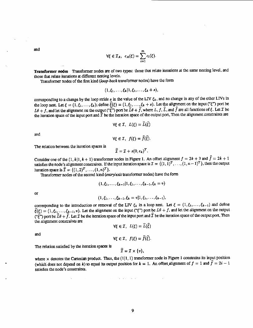
Transformer nodes Transformer nodes are of two types: those that relate iterations at the same nesting level, andthose that relate iterations at differcmt nesting levels.

Transformer nodes of the first kind (loop-back transformer nodes) have the form

(l,_1,.--,_kll,_l,...,_t+s),

corresponding to a change by the loop stride s in the value of the LIV _, and no change in any of the other LIVs in

the loop nest. Let _ = (1, _1, ..., _k); define ((_) = (1, _1, ..., _k + s). Let the align^ment on the input ("C') port beLO + f, and let the alignment on the outEut ("_") port be 1,0 + f, where L, f, L, and f are all functions of _. Let 27bethe iteration space of the input port and 2; be the iteration space of the output port, Then the alignment constraints are

A

k/_ 6 Z, L(_) = L(_)

andA A

ez,fff)=/if).

The relationbetweentheiterationspacesis= Z + s(0,ek)r.

Consider one of the (1, k Il, k + 1) transformer nodes in Figure 1. An offset alignment f = 2k + 3 and f" = 2k + 1satisfies the node's alignment constraints. If the input iteration space is :r = {(1, 1)r ..., ( 1, n - 1)r }, then the output

iteration space is 2" = {(1,2)r,..., (1, n)r}.Transformer nodes of the second kind (entry/exit transformer nodes) have the form

(1,51,...,Sk-dl,Sl,.--,Sk-l,Sk=V)

or

(1,_i,...,_k-l,_k = v11,51,...,5k-1),

corresponding to the introduction or removal of the LIV _k in a loop nest. Let 5 = (1,_1,... ,_-1) and define

_'(_) = (1, _1,.. • •, _k, 1, v). Im the alignment on the input ("_") port be LO + f, and let the alignment on the output("_') port be LO + ]'. Let Z be the iteration space of the input port and _ be the iteration space of the output port, Then

the alignment constraints are

and

The relation satisfied by the iteration spaces is

A

¥_ C 27, L(_) = L(_)

V_ • 2", f(_) -- f(_).

= z x {v},

where x denotes the Cartesian product. "Fnus, the (111, 1) transformer node in Figure 1 constrains its input position

(which does not depend on k) to equal its output position for k = 1. An offset alignment of f = 1 and f = 2i - Isatisfies the node's constraints.

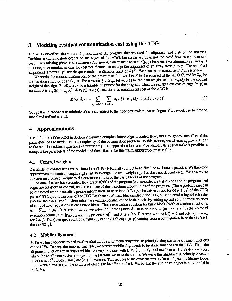
3 Modeling residual communication cost using the ADG

The _ describes the structural properties of the program that we need for alignment and distribution analysis.Residual communication occurs on the edges of the/kiN], but s0f_ we_have not indicated how to estimate thiscost. This missing piece is the distance function d, where the distance d(p, q) between two alignments p and q is

a nonnegative number giving the cost per element to change the alignment of an array from p to q. The set of allalignments is normally a metric space under the distance function d [3]. We discuss the structure of d in Section 4.

We model the communication cost of the program as follows. Let E be the edge set of the ADG G, and let 27xybe

the iteration space of edge (z, y). For a vector _ in Z_y, let w_y(_) be the data weight, and let c_y(_) be the controlweight of the edge. Finally, let _rbe a feasible alignment for the program. Then the realignment cost of edge (x, y) atiteration _ is c_y(_) •w_(_) •d(Tr_(_), % (_)), and the total realignment cost of the ADG is

a, = (1)

Our goal is to choose r to minimize this cost, subject to the node constraints. An analogous framework can be used tomodel redistribution cost.

4 Approximations

The definition of the ADG in Section 2 assumed complete knowledge of control flow, and also ignored the effect of the

parameters of the model on the complexity of the optimization problem. In this section, we discuss approximationsto the model tO address questions of practicality. The approximations are of two kinds: those that make it possible to

compute the parameters of the model, and those that make the optimization problem tractable.

4.1 Control weights

Our model of control weights as a function of LIVs is formally correct but difficult to evaluate in practice. We therefore

approximate the control weight c_(_) as an averaged control weight c_ that does not depend on _. We now relatethis averaged control weight to the execution counts of the basic blocks of the program.

Assume that we have a control flow graph (CFG) of the program (whose nodes are basic blocks of the program, and

edges are transfers of control) and an estimate of the branching probabilities of the program. (These probabilities canbe estimated using heuristics, profile information, or user input.) Let Pij be this estimate for edge (i, j) of the CFG;

pij = 0 if (i, j) is not an edge of the CFG. Let there be B basic block nodes in the CFG, plus the two distinguished nodesENTER and EX/T. We first determine the execution counts of the basic blocks by setting up and solving"conservation

of control flow" equations at each basic block. The conservation equation for basic block i with execution count ui is

ui = _ #_ Pjiuj. In matrix notation, we solve the linear system Au = v, where u = [ul,. • -, uB]T is the vector ofexecution counts, v = [P_NTER,1, " "", PENTEn,B] T, and A is a B x B matrix with A(i, i) = 1 and A(i, j) = -pji

for i ¢ j. The (averaged) control weight _ of the ADG edge (z, y) coming from a computation in basic block b is

thenudlZ= I.

4.2 Mobile alignment

So far we have not constrained the form that mobile alignments may take. In principle, they could be arbitrary functionsof the LIVs. To keep the analysis tractable, we restrict mobile alignments to be affme functions of the LIVs. Thus, the

alignment function for an object within a k-deep loop nest with LIVs _1,..., _ is of the form ao + a1_1+"" + ak_k,where the coefficient vector a = (ao,. ••, a_) is what we must determine. We write this alignment succinctly in vectornotation as a_ r. Both a and _ are (k + 1)-vectors. This reduces to the constant term ao for an object outside any loops.

Likewise, we restrict the extents of objects to be aftine in the LIVs, so that the size of an object is polynomial in

the LIVs.

10

4.3 Replicated alignments

In Section 2, we introduced triplet offset positions to represent the possibility of replication. In practice, we treat the

replication component of offset separately from the scalar component. The alignment space for replication has twoelements, called R (for replicated) and N (for non-replicated). The extent of replication for an tt alignment is the entire

template extent in that dimension. In this approximate model of replication, communication is required only whenchanging from a non-replicated alignment to a replicated one. Thus, the distance function is given by d(N, R) - 1and d(R, R) = d(R, N) - d(N, N) = 0. We call the process of determining these restricted replicated alignments

replication labeling.

4.4 Distance functions

In introducing the distance function in Section 3, we defined it to be the cost per element of changing from onealignment to another. Now consider the various kinds of such changes, and their communication costs on a distributed-memory machine. A change in axis or stride alignment requires unstructured communication. Such communicationis hard to model accurately as it depends critically on the topological properties of the network (bisection bandwidth),the interactions among the messages (congestion), and the software overheads. Offset realignment can be performed

using shift communication, which is usually substantially cheaper than unstructured communication. Replicatingan object involves broadcasting or multicasting, which typically uses some kind of spanning tree. Such broadcastcommunication is likely to cost more than shift communication but less than unstructured communication.

We could conceivably construct a single distance function capturing all these various effects and their interactions,but this would almost certainly make the analysis intractable. We therefore split the determination of alignments intoseveral phases based on the relative costs of the different kinds of communication, and introduce simpler distance

functions for each of these phases.We determine axis and stride alignments (or the matrix L of Section 2.2) in one phase, using the discrete metric to

model axis and stride realignment. This metric, in which d(p, q) = 0 if p = q and d(p, q) = 1 otherwise, is a crudebut reasonable approximation for unstructured communication.

We determine scalar offset alignment in a separate phase, using the grid metric to model shift realignment. In

this metric, ali_ments are the vectors f of Section 2.2, and d(f, f') )s, the Manhattan distance between them, i.e.,d(f,f') = )"_i=11fi - f'l- Note that the distance between f and is the sum of the distances between theirindividual components. This property of the metric, called separability, allows us to solve the offset alignment

problem independently for each axis [3].Finally, we use yet another phase to determine replicated offsets, using the alignments and distance function

described in Section 4.3.The ordering of these phases is as follows: we first perform axis and stride alignment, then replication labeling,

and finally offset alignment.The various kinds of communication interact with one another. For instance, shifting an object in addition to

changing its axis or stride alignment does not increase the communication cost, since the shift can be incorporated intothe unstructured communication needed for the change of axis or stride. We model such effects in a simple manner,

by introducing apresence weight of an edge for each phase of the alignment process. The presence weight multipliesthe contribution of the edge to the total realignment cost for that phase. Initially, all presence weights are 1. Edgesthat end up carrying residual axis or stride realignment have their presence weights set to zero for the replication andoffset alignment phases. Similarly, edges carrying replication communication have their presence weights set to zerofor the offset alignment phase.

5 Determining alignments using the ADG

In this section, we briefly describe our algorithms for determining alignment. Full descriptions of these algorithms are

in our previous papers [2, 3, 4].

11

5.1 Axis and stride alignment ........

To determine axis and stride alignment, we minimize the communication cost K(G, d, _r) using the discrete metric as

the distance function. The position of a port in this context is the matrix L of the alignment function. The algorithm

we use, called compact dynamlcprogramming [3], works in two phases, k=

In the first phase, we traverse the ADG from sources to sinks, building for each port a cost table indexed by

position. The cost corresponding to position p gives the minimum cost of evaluating the subcomputation up to that

port and placing the result in position p. The cost table at a node can be computed from the cost tables of its inputsand the distance functions. This recurrence is used to build the cost tables efficiently. At the end of the first phase, we

examine the cost tables of the sinks of the ADG and place the sinks at their minimum-cost positions. In the second

phase, we traverse the ADG from sinks to sources, placing the ports so as to achieve the minimum costs calculated in

the first phase.Compact dynamic programming is based on the dynamic programming approach of Mace [12]. The "compact" in

the name refers to the way we exploit properties of the distance function to simplify the computation of costs and to

compactly represent the cost tables. The method is exact if the ADG is a tree, but in general it is an approximation.

5.2 Offset alignment

For offset alignment, a position is the vector f of the alignment function, and the Manhattan metric is the distancefunction. As the distance function is separable, we can solve independently for each component of the vector. For

code where the positions do not depend on any LIVs, the constrained minimization can be solved exactly using

linear programming [2, 4]. With mobile alignments, the residual communication cost can be approximated and this

approximate cost minimized exactly using linear programming.

5.3 Replication labeling

For replication labeling, the position space has two positions for each template axis, called R (for replicated) and N

(for non-replicated). The distance function is as given in Section 4.3. Note that this distance function is not a metric.

The sources of replication are spread operations, certain vector-valued subscripts, and read-only objects with mobile

offset alignment. As in the offset alignment case, each axis can be treated independently.

A minimum-cost replication labeling can be computed efficiently using network flow [2].

6 Comparison with other work

In this section, we compare the ADG representation with SSA form and with the preference graph, another represen-

tation that has been used for automatic determination of alignments.

6.1 SSA form

While our ADG representation is based on SSA form, it has a number of extra features. All of the differences stem from

the fact that the ADG representation was designed to manipulate positions of objects, while SSA form was designed

to manipulate values. In fact, an SSA form based on a nonstandard "position semantics" would probably look exactly

like the AIM} formalism.

The ADG representation annotates the ports and edges with data weights, control weights, and iteration spaces,

none of which are present in SSA form. However, the substantive diffovmce between the two rel_resentations lies in

the nodes. Every _-function of SSA corresponds to a merge node in ADG, but certain merge nodes (e.g., for read-only

objects within a loop) do not correspond to any $-functions in SSA. Similarly, fanout and branch nodes have no analog

in SSA form.The fanout and branch nodes of the AIX} resemble similar nodes in the Program Dependence Web representation

developed by Ballance et al. [1]. However, the motivations behind them are very different.

12

6.2 The preference graph

Another representation that has been used in alignment analysis is the preference graph, which has several variants [7,

10, 11, 14]. The preference graph is an undirected, weighted graph constructed from the reference patterns in the

program. The nodes of the preference graph correspond to dimensions of array occurrences in the program, the edgesreflect beneficial alignment relations, and the weights reflect the relative importance of the edges. The edges of the

preference graph encode axis alignment, while additional node attributes are used to encode stride and offset alignment.

The preference graph has two kinds of edges, corresponding to the two sources of alignment decisions. Each state-

meat considered in isolation provides some relations among nodes that avoid residual communication in computing the

given statement. The edges corresponding to these relations are called conformance preference edges. A conformance

preference edge between two array occurrences indicates that if they are not aligned, residual communication will be

needed to align them in preparation for the operation.

The second kind of alignment preference comes from relating definitions and uses of the same array variable. The

edges corresponding to these relations are called identity preference edges. An identity preference edge between two

array occurrences indicates that if they are not positioned identically, residual communication will be needed to makethe values from the definition available at the use.

Alignment decisions are made by contracting graph edges. At each step, an edge is chosen, and if the two nodes

connected by the edge satisfy certain conditions, the edge is contracted and one of the nodes is merged into the

other. When an edge is contracted, we say that the alignment preference it carries has been honored. The contraction

process stops when no more edges can be contracted. An acyclic preference graph can be contracted to a single

node, guaranteeing a communication-free implementation. If, however, there are cycles in the preference graph, some

alignment preferences may remain unhonored and will result in residual communication. In this case, we must decide

which preferences to honor and which to break. There are two principal variants of this general framework.

The Knobe-Lukas-Steele algorithm Knobe, Lukas, and Steele [10] call the nodes of the preference graph cells.

They introduce an additional attribute of cells (called independence anti-preference) to model the constraint that a

dimension occurrence has sufficient parallelism and should not be serialized.

An alignment conflict can only occur within a cycle of _the preference graph. We therefore need to locate a cycle,determine whether it causes a conflict, and resolve the conflict if it exists. Actually, we only need to examine and

resolve conflicts in a set of fundamental cycles of the preference graph, since if such a cycle basis is conflict-free, then

all cycles in the graph are conflict-free. A cycle basis can be easily determined from a spanning tree of the graph: each

non-tree edge determines a unique fundamental cycle of the graph with respect to the spanning tree. This ignores the

fact that the preference graph is weighted. Given a choice between honoring two preferences, we would choose tohonor the preference with higher weight. The Knobe-Lukas-Steele algorithm uses the nesting depth of an edge as its

weight and constructs a maximum-weight spanning tree.An unhonored identity preference implies that an object will live in distinct location in different parts of the

program. An unhonored conformance preference implies that not all of the operations in a statement are necessarily

performed in the location of the "owner" of the LHS. In other words, breaking a conformance preference is the

mechanism for improving the "owner-computes rule".

The Ll-Chen algorithm Li and Chen [I I] use the preference graph model to determine axis alignment. Their

algorithm was developed in the context of the Crystal language, which allows more general reference patterns than we

have considered, for instance, a pattern like A(i, j) = B(i, i). This indicates conformance preferences between thefirst axis of A and both axes of B; such sets of preferences that are generated from the same reference pattern and arc

incident upon a common node are said to be competing.Li and Chen call the preference graph the Component Affinity Graph (CA(}), and call preferences ajfinities.

Competing edges have weight _,while noncompeting edges are unit-weight. The quantities, and 1 arc incommensurate,

with _ _: 1. The axis alignment problem is framed as the following graph partitioning problem:

Partition the node set of the CAG into n disjoint subsets Vl,..., Vn (where n is the maximum dimension-

ality of any array) with the restriction that no two axes of the same array may be in the same partition, so

as to minimize the sum of the weights of edges connecting nodes in different subsets of the partition.

13

The idea here is to align array dimensions in the samc subset of the par_i'fion,with ed_gesbetween n0des in .dfffem.ntpartitions corresponding to residual communication. Hence the condition that we minimize the sum of the weights of

such edges.The graph partitioning problem stated above is NP-complete [11]. Li and Chen therefore solve it heuristically by

finding maximum-weight matchings of a sequence of bipartite subgraphs of the CAG.

Discussion We now compare the ADG approach with the preference graph approach with regard to semantics, cost

modeling, and the treatment of control flow.

• The conformance preferences, while similar to the node constraints of our approach, are not clearly relatedto thedata flow and the intermediate results of the computation. Intermediate results have no explicit representationin the conformance graph model. They could, however, be made explicit by preprocessing the source.

• The preference graph model distinguishes between objects atdifferent levels of a loop nest, but does not considerthe size of an object, or the shift distance, in computing the cost of moving it. In fact, it can be thought of as

using the unweighted discrete metric to model all communication cost.

• Knobe et al. [113]discuss handling control flow by introducing alignments for arrays at merge points in the

program. Our use of static single assignment form provides a sound theoretical basis regarding the placementof merge nodes.

• To the best of our knowledge, the preference graph method has not been used to determine when objects should

be replicated.

7 Conclusions

We have motivated and described a representation of data-parallel programs called the alignment-distribution graph,which provides a mechanism for explicitly representing and optimizing residual communication cost. The represen-tation is based on a separation of variables and values, extended from the static single assignment form of programs.The communication requirements of the program are faithfully modeled by carefully representing realignment com-munication due to control flow, loop-carried dependences, assignment to sections of arrays, and transformational array

operations.The ADG provides a more detailed model of residual communication than the preference graph, another represen-

tation that has been used for the same analysis. We have developed algorithms in the ADG framework to determine

axis alignment, mobile stride and offset alignment, and replication. We have devised a scheme for generating theADG from program text, which we are presently refining and implementing. We are also implementing the algorithmsmentioned in Section 5 to test the validity of this approach.

We are currently studying several interesting problems that remain unsolved. These include developing algorithmsfor distribution analysis using the ADG framework, understanding the interactions between the alignment and dis-tribution phases, developing interprocedural optimization techniques in this framework, finding better algorithms forsolving the alignment problem in the discrete metric, and allowing for the possibility of skew alignments.

References

[1] Robert A. Ballance, Arthur B. Maccabe, and Karl J. Ottenstein. The Program Dependence Web: A representation

supporting control-, data-, and demand-driven interpretation of imperative languages. In Proceedings of the ACMSIGPLAN'90 Conference on Programming Language Design and Implementation, pages 257-271, White Plains,NY, June 1990.

[2] Siddhartha Chatterjee, John R. Gilbert, and Robert Schreiber. Mobile and replicated alignment of arrays indata-parallel programs. In Proceedings of Supercomputing'93, Portland, OR, November 1993. To appear.

14

[3] Siddhartha Chatterjee, John R. Gilbert, Robert Schreiber, and Shang-Hua Teng. Optimal evaluation of array

expressions on massively parallel machines. In Proceedings of the Second Workshop on Languages, Compilers,

and Runtime Environments for Distributed Memory MuItiprocessors, Boulder, CO, October 1992. Published in

SIGPLAN Notices, 28(I), January 1993, pages 68-71. An expanded version is available as RIACS Technical

Report TR 92.17 and Xerox PARC Technical Report CSL-92-11.

[4] Siddhartha Chatterjee, John R. Gilbert, Robert Schreiber, and Shang-Hua Teng. Automatic array alignment

in data-parallel programs. In Proceedings of the l_¢entieth Annual ACM SIGACTISIGPLAN Symposium on

Principles of Programming Languages, pages 16-28, Charleston, SC, January 1993. Also available as RIACS

Technical Report 92.18 and Xerox PARC Technical Report CSL-92-13.

[5] Ron Cytron, Jeanne Ferrante, Barry K. Rosen, Mark N. Wegman, and E Kenneth Zadeck. Efficiently computing

static single assignment form and the control dependence graph. ACM Transactions on Programming Languages

and Systems, 13(4):451-490, October 1991.

[6] Geoffrey C. Fox, Seema I-Iiranandani, Ken Kennedy, Charles Koelbel, Uli Kremer, Chau-Wen Tseng, and Min-You Wu. Fortran D language specification. Technical Report Rice COMP TR90-141, Department of Computer

Science, Rice University, Houston, TX, December 1990.

[7] Manish Gupta. Automatic Data Partitioning on Distributed Memory Multicomputers. PhD thesis, University ofIllinois at Urbana-Champaign, Urbana, IL, September 1992. Available as technical reports UILU-ENG-92-2237

and CRHC-92-19.

[8] High Performance Fortran Forum. High Performance Fortran language specification version 1.0. Draft, January1993. Also available as technical report CRPC-TR 92225, Center for Research on Parallel Computation, Rice

University.

[9] Richard Johnson and Keshav Pingali. Dependence-based program analysis. In Proceedings of the ACM SIG-

PLAN'93 Conference on Programming Language Design and Implementation, pages 78-89, Albuquerque, NM,

June 1993.

[10] Kathleen Knobe, Joan D. Lukas, and Guy L. Steele Jr. Data optimization: Allocation of arrays to reducecommunication on SIMD machines. Journal of Parallel and Distributed Computing, 8(2): 102-118, February

1990.

[11] Jingke Li and Marina Chen. The data alignment phase in compiling programs for distributed-memory machines.

Journal of Parallel and Distributed Computing, 13(2):213-221,October 1991.

[12] Mary E. Mace. Memory Storage Patterns in Parallel Processing. Kluwer international series in engineering and

computer science. Kluwer Academic Press, Norwell, MA, 1987.

[13] Thinking Machines Corporation, Cambridge, MA. CM Fortran Reference Manual Versions 1.0 and 1.1, July

1991.

[14] Skef Wholey. Automatic Data Mapping for Distributed-Memory Parallel Computers. PhD thesis, School of

Computer Science, Carnegie Mellon University, Pittsburgh, PA, May 1991. Available as Technical Report

CMU-CS-91-121.

[15] Pavel Winter. Steiner problem in networks: A survey. Networks, 17:129-167, 1987.

15

II

RIACSMail Stop T041-5

NASA Ames Research Center

Moffett Field, CA 94035