The University of Maine The University of Maine

DigitalCommons@UMaine DigitalCommons@UMaine

Honors College

Spring 5-2018

The Analysis of Labor Market Efficiency: A Comparative Analysis The Analysis of Labor Market Efficiency: A Comparative Analysis

of Maine and the United States of Maine and the United States

Sarah M. Welch University of Maine

Follow this and additional works at: https://digitalcommons.library.umaine.edu/honors

Part of the Finance Commons

Recommended Citation Recommended Citation Welch, Sarah M., "The Analysis of Labor Market Efficiency: A Comparative Analysis of Maine and the United States" (2018). Honors College. 361. https://digitalcommons.library.umaine.edu/honors/361

This Honors Thesis is brought to you for free and open access by DigitalCommons@UMaine. It has been accepted for inclusion in Honors College by an authorized administrator of DigitalCommons@UMaine. For more information, please contact um.library.technical.services@maine.edu.

THE ANALYSIS OF LABOR MARKET EFFICIENCY: A COMPARATIVE

ANALYSIS OF MAINE AND THE UNITED STATES

by

Sarah M. Welch

A Thesis Submitted in Partial Fulfillment of the Requirements for a Degree with Honors

(Financial Economics)

The Honors College

University of Maine

May 2018

Advisory Committee: Andrew Crawley, Assistant Professor of Economics, Advisor James Breece, Associate Professor of Economics Angela Daley, Assistant Professor of Economics Todd Gabe, Professor of Economics Jordan LaBouff, Associate Professor of Psychology, Honors College

© 2018 Sarah M. Welch

All Rights Reserve

ABSTRACT

The purpose of this research is to analyze the change in the labor market

efficiency from before to after the great recession and its effect on economic output

following the recession. Concerns have been raised about the adjustment of the labor

market compared to the recovery of other economic indicators. Influenced by the

methods of Blanchard and Diamond (1989) and Dixon et al. (2014), the Beveridge curve

and matching function are used to estimate and observe changing labor market dynamics

through the relationship between unemployment and job vacancies.

This thesis finds that labor markets for both Maine and the United States are less

efficient after the recovery period than they were prior to the recession. There is also

evidence indicating that in 2015 and 2016 Maine has a more efficient labor market than

the United States. Possible reasons for the lower labor market efficiencies are the lower

labor force participation, automation, and the distribution of vacancies across industries.

Future research will consist of measuring the influence of labor market efficiency as well

as applying the Beveridge curve and matching function across all states.

iv

TABLE OF CONTENTS

I. Introduction 1 Introduction 1 Research Objective 4 II. Literature Review 5 Theoretical Supply and Demand of Labor 5 Job Search Theory 7 Approach to Labor Market Efficiency Analysis: The Beveridge Curve 10 Approach to Labor Market Efficiency Analysis: The Matching Function 13 Empirical Applications in the United States 19 III. Data and Methodology 23 Methodology 23 The Approach of this Thesis 24 Data 26 Table of Variables 29 Theoretical Beveridge Curve 30 IV. Empirical Findings 32 Maine’s Beveridge Curve and Labor Market Efficiency 32 United States’ Beveridge Curve and Labor Market Efficiency 36 A Case Study on Output and the Labor Market Efficiency 40 V. Discussion of Findings 42 Direct Comparison and Contrast 42 Potential Causes for the Behavior of the Matching Efficiency 46 VI. Conclusion 52 Works Cited 54 Appendix A 58 Appendix B 59 Appendix C 60 Appendix D 61 Author’s Biography 62

v

TABLE OF TABLES AND FIGURES

I. Tables Table 1. Critical Variables 29 Table 2. VAR Results from Stata 41 Table 3. Vacancies by Industry in Maine 50

II. Figures Figure 1. Maine Labor Market Quarterly Changes 2 Figure 2. United States Labor Market Quarterly Changes 3 Figure 3. Quantity of Labor and Wages. From Hansen (1970) 9 Figure 4. Theoretical Beveridge Curve. From Dow and Dicks-Mireaux (1958) 11 Figure 5. Theoretical Beveridge Curve. From Hansen (1970) 12 Figure 6. Theoretical Beveridge Curve. From Dixon et al. (2014) 16 Figure 7. The Adjusted Normalized Help-Wanted Index and Unemployment 20 Figure 8. Change in the Beveridge Curve. From Cahuc and Zylberberg (2004) 26 Figure 9. Theoretical Beveridge Curve 30 Figure 10. Maine Beveridge Curve 32 Figure 11. Maine Matching Efficiency 33 Figure 12. Maine Beveridge Curve and Matching Efficiency 35 Figure 13. United States Beveridge Curve 36 Figure 14. United States Matching Efficiency 37 Figure 15. United States Beveridge Curve and Matching Efficiency 39 Figure 16. Impulse Response Function from Stata 41 Figure 17. The Beveridge Curve 43 Figure 18. Matching Efficiency 45 Figure 19. Labor Force Participation Rate of Maine and the United State 46 Figure 20. Percent Change in Annual Real GDP 48

1

INTRODUCTION

The initial motivation for this thesis was based upon a question of how efficient

Maine’s labor market is, as there have been growing concerns for Maine’s economy

overall. Currently, Maine’s unemployment is low and is on par with the rest of the United

States. Some regions in Maine, specifically the Cumberland and York county area, have

an unemployment rate under 3% as reported by the Maine Department of Labor. But, is

this unemployment statistic low because the labor market is healthy, or is it low because

the number of people looking for work has decreased due to so many people leaving the

labor market? If it is the latter, evidence could appear in measurements of labor market

efficiencies; specifically, when comparing the people who are unemployed to the jobs

that are vacant and how well these two groups are being matched.

After getting an idea of Maine’s labor market health, it is then important to

compare to the higher aggregate level of the United States. Throughout the recovery

period there were concerns regarding the United States’ economy getting back up to pace

since the recession; concerns mostly due to the slow growth rate and the fact that many

workers were getting discouraged and exiting the labor force1. Beginning in 2014,

Americans did start regaining their confidence in the economy, as more jobs were

1 Doughtery, C. (2011). Slow Growth Stirs Fears of Recession. Retrieved February 4, 2018, from

https://www.wsj.com/articles/SB10001424053111904800304576475811201857064?mod=searchresults&page=1&pos=15

2

opening and GDP began to rise at a faster rate2. But, was the labor market as healthy as it

seemed, and is it fully recovered now?

To get an idea of the recovery of the overall labor market conditions for Maine

and the United States, the seasonally-adjusted quarterly changes in the labor market,

(shown in blue), employment (shown in green), and unemployment (shown in red), from

2006 through 2016 are presented in figures 1 and 2. The data is from the Bureau of Labor

Statistics’ Current Population Survey (CPS) and the and Local Area Unemployment

Statistics (LAUS).

Figure 1. Maine Labor Market Quarterly Changes

2 At Last, a Proper Recovery. (2015, February). The Economist. Retrieved from

https://www.economist.com/news/united-states/21643196-all-sorts-americans-are-feeling-more-prosperous-last-proper-recovery

-4000

-3000

-2000

-1000

0

1000

2000

3000

2006

q2

2006

q4

2007

q2

2007

q4

2008

q2

2008

q4

2009

q2

2009

q4

2010

q2

2010

q4

2011

q2

2011

q4

2012

q2

2012

q4

2013

q2

2013

q4

2014

q2

2014

q4

2015

q2

2015

q4

2016

q2

2016

q4

Maine Quarterly Changes (Levels)

Labor Force Employment Unemployment

3

Figure 2. United States Labor Market Quarterly Changes

During the peak of the recession, both graphs show almost identical trends of a

sharp increase in unemployment, a sharp decrease in employment, and a labor force that

is relatively constant. However; what is interesting are the differences that occur during

the recovery period. For Maine, from the third quarter of 2013 through the third quarter

of 2015 the unemployment level in Maine is decreasing, which is good, but meanwhile

the employment level and labor force are also decreasing for eight consecutive quarters.

For the United States, the labor market picture does tell a story of recovery, but a slow

recovery.

To further understand the dynamics of labor markets it is critical to analyze and

observe trends in the relationships between the labor market variables over time.

Unemployment rates are often looked upon as a one of the measurements used to

-1000

-800

-600

-400

-200

0

200

400

600

800

2006q2

2006q4

2007q2

2007q4

2008q2

2008q4

2009q2

2009q4

2010q2

2010q4

2011q2

2011q4

2012q2

2012q4

2013q2

2013q4

2014q2

2014q4

2015q2

2015q4

2016q2

2016q4

United States Quarterly Changes (Levels in Thousands)

Labor Force Employment Unemployment

4

determine how healthy the economy is as a whole. Since the peak of the great recession,

the unemployment rate has successfully returned to a low value in Maine and the United

States. But, does this mean that the labor market in each region is healthy and efficient?

Research Objective

• Output increases as the labor market becomes more efficient.

• The labor markets for Maine and the United States are not as efficient post-

recovery as they were pre-recession.

The first research objective presents a testable hypothesis and is included in this

thesis. However, this work moves beyond this one simple hypothesis. The tools that the

thesis will use to estimate the efficiency of the labor markets are the Beveridge Curve and

the Matching Function. At a glance, the Beveridge Curve relates unemployment rates and

job vacancy rates and can pick up on cyclical and structural trends in the labor market,

which can be paired with the Matching Function and used to estimate the labor market

efficiency. Both of the Beveridge curves and the matching efficiencies for Maine and the

United States can be compared to themselves across time and to each other, thus being

able to address the second research objective.

5

LITERATURE REVIEW

Theoretical Supply and Demand of Labor

In economics there is a large focus on supply and demand analysis, whether that

be in terms of goods, services, or labor. In this thesis, the focus is on the supply and

demand of labor. The neoclassical theory of labor supply states that individuals face a

trade-off between hours of work and hours of leisure (Cahuc and Zylberberg, 2004). In

terms of deciding how much work and how much leisure, individuals often look to wages

and make decisions based on their reservation wage, which is the minimum wage a

worker will accept. Under general conditions, the reservation wage is a function of search

costs, job offers, and the distribution of wage offers (Addison et al., 2013). If the current

wage is equal to or greater than the reservation wage labor supply will be positive and the

marginal rate of substitution between consumption and leisure is equal to the hourly wage

(Cahuc and Zylberberg, 2004).

According to this theory, the labor force participation rate corresponds to the

proportion of individuals who have a reservation wage less than the current wage. The

labor force participation also resembles labor supply and the unemployment rate is the

difference between the supply curve and the demand curve. However, many economists

do not fully agree with the labor supply model when comparing it to wages.

Blanchflower and Oswald (1994) wage curve reflects that high unemployment

corresponds with a low wage rate, which is reverse from the proposed neoclassical

theory. They argue that unemployment is more of a gap between labor supply and a fixed

labor force, rather than the gap between supply and demand as long as the potential labor

6

force is a fixed number above the market clearing rate, essentially the reservation wage

(Blanchflower and Oswald, 1994).

In terms of labor demand theory, there exists both conditional demand and

unconditional demand. Conditional demand refers to the quantities of each input that a

firm desires to utilize to attain a given level of output. Unconditional demand refers to

when a firm wants to maximize their profits and will demand the optimal quantities of

each input in order to do so (Cahuc and Zylberberg, 2004). Since labor is an input for a

firm, both the conditional and unconditional demand for labor follow the law of demand.

Meaning, labor demand always decreases when the cost of labor increases. The cost of

labor can be interpreted as wages, therefore the market where supply and demand of

labor meet is in terms of quantity of labor and wages. In terms of behavior, when the

wage rate is above the equilibrium level the demand curve represents employment. When

the wage rate is below equilibrium, the supply curve represents employment (Hansen,

1970). Although, this assumes that the labor market is homogeneous and in a frictionless

state.

The limitation in the well-behaved supply and demand framework is that labor

markets are neither homogeneous nor frictionless and as a result the theoretical model is

limited. In addition, there are two main conditions that deter labor from behaving like a

standard input for a firm. The first is that the workers retain ownership of their human

capital and the second is that the workers must be present to have their skills used by the

firm (Booth, 2014). Essentially, labor markets are far from perfectly competitive, but

using perfectly competitive theory can help understand the underlying dynamics.

Ultimately, efficient contracts for workers are on the labor demand curve (Oswald, 1993).

7

Job Search Theory

The theoretical labor supply presented above does help explain why there should

be unemployed people looking for work (Cahuc and Zylberberg, 2004), since this

category of the population has no reason to exist in a universe where information is

symmetric, and markets clear perfectly under a centralized market system for firms and

workers to meet (Rogerson et al., 2005). Job search theory was introduced to better

understand the complexities of the matching process. It works by assuming that

individuals know only the distribution of wages existing in the economy, and they must

search in order to encounter employers who will make them definite wage offers (Cahuc

and Zylberberg, 2004). The job search function is paired with job search theory, and

looks more in depth at why some workers choose to remain unemployed.

In the literature, a basic job search function in discrete time is shown where the

worker wants to maximize expected income denoted as: E∑ 𝛽#𝑥#%#&' , which is calculated

based upon income minus a discount factor 𝛽 ∈ (0,1) (Rogerson et al, 2005). This is the

same as maximizing expected utility if the worker is risk neutral. In this expectation, 𝑥# is

the worker's income at time t. If the worker is employed at wage w, 𝑥 = 𝑤. If a worker is

unemployed, 𝑤 = 𝑏 where b > 0 and represents unemployment insurance.

A way of looking at a solution to this problem is by using dynamic programming

techniques such as the Bellman Equations (Bellman, 1955). Here, they display the payoff

from working as well as the payoff from remaining unemployed (Rogerson et al., 2005).

The initial equations from Rogerson et al. (2005) are:

(1) 𝑊(𝑤) = 𝑤 + 𝛽𝑊(𝑤)

(2) 𝑈 = 𝑏 + 𝛽 ∫ 𝑚𝑎𝑥{𝑈,𝑊(𝑤)}𝑑𝐹(𝑤)%'

8

In equation 1, W(w) is the payoff by accepting wage w and U is the payoff from

rejecting wage w. In equation 2, F(w) is a known distribution of wages in the market. By

rearranging equation 1, we find that W(w) is always increasing.

(3) 𝑊(𝑤) = =>?@

The Bellman Equations can also be observed using continuous time where the

length of one period is 𝛥 and 𝛽 = >>?BC

. The new Bellman Equations with continuous

time are now:

(4) 𝑟𝑊(𝑤) = (1 + 𝑟𝛥)𝑤

(5) 𝑟𝑈 = (1 + 𝑟𝛥)𝑏 + 𝛼 ∫ 𝑚𝑎𝑥{0,𝑊(𝑤) − 𝑈}𝑑𝐹(𝑤)%'

In equation 5, 𝛼𝛥 is the probability that the unemployed worker gets a wage offer in each

period. When 𝛥 → 0 these equations become:

(6) 𝑟𝑊(𝑤) = 𝑤

(7) 𝑟𝑈 = 𝑏 + 𝛼 ∫ 𝑚𝑎𝑥{0,𝑊(𝑤) − 𝑈}𝑑𝐹(𝑤)%'

In equation 7, rU is the flow value of the unemployment payoff per period, b is the

instantaneous payoff and the last term is the expected value of any changes in the value

of the worker’s state (Rogerson et al. 2005).

The optimal strategy for a job seeker consists of accepting any wage offer higher

than his or her reservation wage that occurs where W(𝑤H) = U. At any point below the

reservation wage, the job searcher would benefit more by remaining unemployed and

only receiving the unemployment insurance. Rogerson et al. (2005) presents the

reservation wage in continuous time as:

(8) 𝑤H = 𝑏 +IB ∫ [1 − 𝐹(𝑤)]𝑑𝑤%

=L

9

The job search function can also give insight into how the level of unemployment

insurance affects wages. If unemployment insurance increases, the parameter b will

increase, thus, increasing the reservation rate 𝑤H (Rogerson et al., 2005). Intuitively

reservation wages imply that unemployment insurance generates an increased utility for

those unemployed without changing their employment status; therefore, they begin to

demand a higher wage in order to accept a job offer.

For the firm, job search theory shows that given a pool of workers who cannot

change in the short run, there will be employers who do not find sufficient workers to fill

their demands. Figure 3 shows the theoretical supply and demand curves (𝑆N and 𝐷N) as

well as a third curve (𝐸N) representing the level of employment corresponding with

different wage levels.

Figure 3. Quantity of Labor and Wages. From Hansen (1970).

When wages are low, there is a high demand for labor, but little supply of labor,

and an even smaller amount of labor employed. As wages increase, the supply of labor

10

increases as well, but demand decreases. As for employment, the maximum amount of

labor employed will occur at the equilibrium wage where the theoretical supply and

demand curves intersect. Graphically, the fact that employment, 𝐸N𝐸N, is always to the left

of demand for labor, 𝐷N𝐷N, the demand for labor always exists. The horizontal distance

between 𝐷N𝐷N and 𝐸N𝐸Nmeasures the number of vacant jobs, or excess demand for

employment (Hansen, 1970).

An Approach to Labor Market Efficiency Analysis: The Beveridge Curve

Paired with unemployment, job vacancies can be a tool used to analyze labor

demand and the efficiency of a labor market. Unfilled vacancies exist even while

unemployment exists, implying that the labor demanded differs from the labor supplied,

creating maladjustment caused by various factors including skill and geographical

mismatch (Dow and Dicks-Mireaux, 1958). By plotting vacancies against unemployment,

often in the form of rates, two critical observations can be made. The first allows cyclical

trends in the demand for labor to be captured, the second is the possible early signs of

structural disequilibrium in the labor market to be seen. The relationship between

unemployment and vacancies can be observed graphically on the Beveridge curve. They

have an inverse relationship since they move in opposite cyclical frequencies (Elsby et

al., 2015). Figure 4 is a theoretical Beveridge curve which shows the inverse relationship

between unemployment and vacancies along with what changes in the curve imply for

the labor market being modeled (Dow and Dicks-Mireaux, 1958).

11

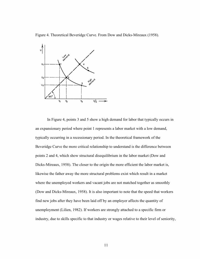
Figure 4. Theoretical Beveridge Curve. From Dow and Dicks-Mireaux (1958).

In Figure 4, points 3 and 5 show a high demand for labor that typically occurs in

an expansionary period where point 1 represents a labor market with a low demand,

typically occurring in a recessionary period. In the theoretical framework of the

Beveridge Curve the more critical relationship to understand is the difference between

points 2 and 4, which show structural disequilibrium in the labor market (Dow and

Dicks-Mireaux, 1958). The closer to the origin the more efficient the labor market is,

likewise the father away the more structural problems exist which result in a market

where the unemployed workers and vacant jobs are not matched together as smoothly

(Dow and Dicks-Mireaux, 1958). It is also important to note that the speed that workers

find new jobs after they have been laid off by an employer affects the quantity of

unemployment (Lilien, 1982). If workers are strongly attached to a specific firm or

industry, due to skills specific to that industry or wages relative to their level of seniority,

12

they are more reluctant to search for employment in other sectors. Ultimately, slowing

down the process of labor adjustment to sectoral shifts (Lilien, 1982).

Similarly, Hansen (1970) plots a Beveridge curve using vacancies derived from

Figure 3 and unemployment data. Unlike Dow and Dicks-Mireaux (1958), Hansen (1970)

places unemployment on the horizontal axis and vacancies on the vertical, but the

theoretical framework remains unchanged.

Figure 5. Theoretical Beveridge Curve. From Hansen (1970).

Hansen (1970) estimates the equation of the Beveridge curve in Figure 6 to be:

(9) 𝑣 = ℎ >S; ℎ > 0

The coefficient h is a measure of structural disequilibrium in the labor market, or the

‘maladjustment’ that Dow and Dicks-Mireaux (1958) discuss (Hansen, 1970). As h

increases the Beveridge curve shifts out and represents a less efficient labor market,

matching the theory of the movement from point 2 to point 4 in Figure 4 (Dow and

13

Dicks-Mireaux, 1958). The inverse relationship between unemployment and vacancies

shows that the “relationship between job openings and jobseekers has been shown to

have fundamental implications for the efficiency of the matching process that generates

employment relationships, and for the nature of shocks that drive fluctuations in the labor

market” (Elsby et al., 2015).

Empirical analysis has been done in multiple countries such as Great Britain

(Dow and Dicks-Mireaux, 1958), Australia (Hagger, 1970), and the United states

(Abraham, 1987; Blanchard and Diamond, 1989), that confirm the theory of cyclical and

structural changes to the Beveridge Curve presented in Figures 4 and 5.

Abraham (1987) and Blanchard and Diamond (1989) observed a labor market in

the United States where the matching process between unemployed workers and job

vacancies was worsening over time and an excess supply of labor resulting from

structural disequilibrium. These findings suggest that there are outside factors such as the

skill level of the workers available, the age of the workers available, and geographical

restrictions that are impacting the supply and demand for labor and causing inefficiencies

more than they have before.

An Approach to Labor Market Efficiency Analysis: The Matching Function

The matching function presented in this body of literature allows for the analysis

of the relationship between unemployment, vacancies, and new hires in a functional

form. Part of this analysis includes recognizing inefficiencies, or mismatch, in the labor

market as it reveals frictions in otherwise conventional models but typically does not

explicitly reference the source of the friction. (Petrongolo and Pissarides, 2001).

14

Mismatch as an empirical concept “measures the degree of heterogeneity in the labor

market across a number of dimensions, usually restricted to skills, industrial sector, and

location” (Petrongolo and Pissarides, 2001).

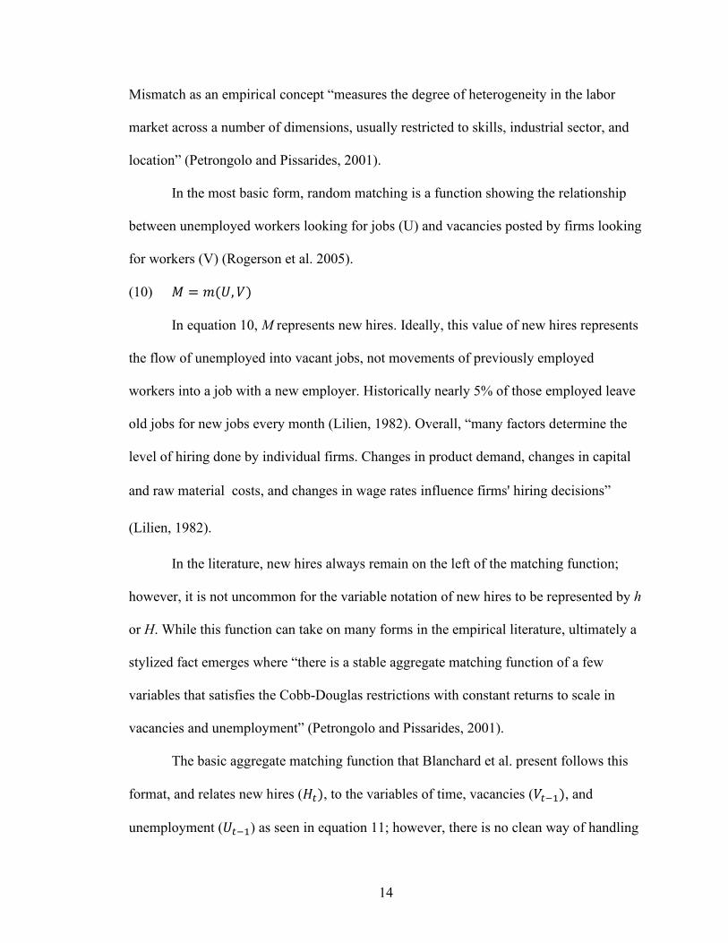
In the most basic form, random matching is a function showing the relationship

between unemployed workers looking for jobs (U) and vacancies posted by firms looking

for workers (V) (Rogerson et al. 2005).

(10) 𝑀 = 𝑚(𝑈, 𝑉)

In equation 10, M represents new hires. Ideally, this value of new hires represents

the flow of unemployed into vacant jobs, not movements of previously employed

workers into a job with a new employer. Historically nearly 5% of those employed leave

old jobs for new jobs every month (Lilien, 1982). Overall, “many factors determine the

level of hiring done by individual firms. Changes in product demand, changes in capital

and raw materialcosts, and changes in wage rates influence firms' hiring decisions”

(Lilien, 1982).

In the literature, new hires always remain on the left of the matching function;

however, it is not uncommon for the variable notation of new hires to be represented by h

or H. While this function can take on many forms in the empirical literature, ultimately a

stylized fact emerges where “there is a stable aggregate matching function of a few

variables that satisfies the Cobb-Douglas restrictions with constant returns to scale in

vacancies and unemployment” (Petrongolo and Pissarides, 2001).

The basic aggregate matching function that Blanchard et al. present follows this

format, and relates new hires (𝐻#), to the variables of time, vacancies (𝑉#?>), and

unemployment (𝑈#?>) as seen in equation 11; however, there is no clean way of handling

15

time and the basic specification is a continuous time model with discrete time data

(Blanchard et al., 1989).

(11) ln(𝐻#) = 𝑎' + 𝑎>𝑡𝑖𝑚𝑒 + 𝑎^ ln(𝑉#?>) + 𝑎_ ln(𝑈#?>) + 𝜖#

“The new hires number for time t corresponds roughly, however, to the integral of the

flow from the middle of month (t - 1) to the middle of month t. The vacancy number for

time t is the integral of the stocks of help-wanted ads over month” (Blanchard et al.,

1989).

The form of Equation 11 is incredibly useful as it is a Cobb-Douglas form; but,

taking a regression in the log form to solve for the parameters will result in parameters

that represent elasticities. This provides a great amount of insight on the dynamics of the

job-matching process in a labor market. Blanchard et al. (1989) estimate these models

and find that both unemployment and vacancies are significant in the hiring process

which poses a contrast to macroeconomic models that often assume only the demand side

determines the rate of hiring.

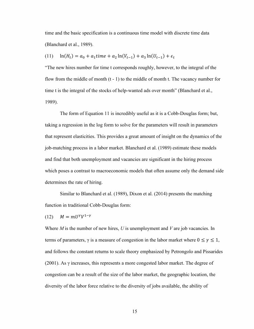
Similar to Blanchard et al. (1989), Dixon et al. (2014) presents the matching

function in traditional Cobb-Douglas form:

(12) 𝑀 = 𝑚𝑈a𝑉>?a

Where M is the number of new hires, U is unemployment and V are job vacancies. In

terms of parameters, γ is a measure of congestion in the labor market where0 ≤ 𝛾 ≤ 1,

and follows the constant returns to scale theory emphasized by Petrongolo and Pissarides

(2001). As γ increases, this represents a more congested labor market. The degree of

congestion can be a result of the size of the labor market, the geographic location, the

diversity of the labor force relative to the diversity of jobs available, the ability of

16

‘outsiders’ to compete with ‘insiders’, and the number of employed seeking job-to-job

movements (Dixon et al., 2014).

Dixon et al. (2014) does well converting the matching function into an equation

that is representative of the Beveridge curve in a clear mathematical manipulation of

Equation 12. Accounting for the size of the labor force in Equation 12, the matching

function can be re-written as:

(13) def= 𝑚( g

ef)a( h

ef)>?a

In this form, it becomes easier to see how the matching function and the Beveridge curve

are related. Using equation 13, Dixon et al. (2014) bring in the concept of the finding

rate, g; which is equal todef

. Now, by manipulating the matching function we find the

Beveridge curve relating gef

and hef

is:

(14) gef= (i

j)kl( hef)m(kml)

l

The graphical representation of Equation 14 is shown in Figure 6 (Dixon et al., 2014).

Figure 6. Theoretical Beveridge Curve. From Dixon et al. (2014).

17

An important thing to note about Equation 14 is that g, the finding rate, varies

with the business cycle. This leads to the intercept in Figure 4 also varying over the

business cycle as it is dependent on both the finding rate (g) and the efficiency of

matching (m) (Dixon et al., 2014). Conceptually, shifts in the Beveridge Curve represent

“how competently the unemployed search for work, how well-suited employers believe

the unemployed are for the available vacancies, and the degree of mismatch between the

skills of the unemployed and the requirements of employers” (Dixon et al. 2014). This is

crucial because analyzing the Beveridge Curve for a specific region gives us the ability to

observe how efficient the labor market is in terms of job search. In Figure 4, the

equilibrium unemployment rate is represented by the 45º line where gef= h

ef, or more

simply as𝑢 = 𝑣.

The matching function can also be useful for looking at flow dynamics in

unemployment and vacancies (Blanchard et al., 1989). Blanchard et al. (1989) presents

the equations of motion where basic labor market flow identities are combined with the

matching function to yield a system of equations that represent the behavior of the labor

market. The first basic identity is:

(15) 𝐿 = 𝐸 + 𝑈

Where L represents the labor force, E is the number of employed workers, and U is the

number of unemployed workers. The second identity in their introductory model is:

(16) 𝐾 = 𝐹 + 𝑉 + 𝐼

Where K is the total number of jobs, F is the number of filled jobs, V is the number of

vacancies, and I is the number of idle jobs, which represents jobs that are unfilled, but no

vacancies are posted. “We think of each of the K jobs in the economy as producing, if

18

filled a gross (of wages) revenue of either 1 or 0. Profitability for each job follows a

Markov process in continuous time. A productive job becomes unproductive with a flow

probability of 𝜋'. An unproductive job becomes productive with flow probability

𝜋>”(Blanchard et al. 1989).

The final piece of information needed to introduce the equations of motion is that

workers quit their jobs at an exogenous rate represented by the constant q. It is to be

noted that a quit is different from a job termination as a quit is connected to the posting of

a new vacancy and a termination is not. Blanchard et al. (1989) models the behavior of

the labor market as a system of two differential equations3:

(17) sts#= 𝛼𝑚(𝑈, 𝑉) − 𝑞𝐸 −𝜋'𝐸

(18) shs#= −𝛼𝑚(𝑈, 𝑉) + 𝑞𝐸 + 𝜋>𝐼 −𝜋'𝑉

Equation 17 gives the flow of employment while equation 18 gives the flow of vacancies.

Then, using identities provided in previous equations, this system can be rewritten as a

system of unemployment in vacancies.

(19) sgs#= −𝛼𝑚(𝑈, 𝑉) +(𝑞 + 𝜋')(𝐿 − 𝑈)

(20) shs#= −𝛼𝑚(𝑈, 𝑉) +(𝑞 − 𝜋>)(𝐿 − 𝑈) +𝜋>𝐾 −(𝜋' + 𝜋>)𝑉

In equations 19 and 20, the negative matching function shows that an increase in new

hires will decrease the level of vacancies and unemployment; but, there exists additional

influences on the changes in vacancies and unemployment besides what is captured in the

matching function. Therefore, the theory follows that the matching function is a

3Blanchard et al. (1989) defines the matching function as: ℎ = 𝛼𝑚(𝑈, 𝑉). Where h represents new hires and a is a scale parameter. Changes in the parameter are intended to capture changes in the geographic region, skill characteristics, and/or search behavior that differ over workers and new vacancies.

19

significant part of labor market flows but alone does not capture the entire dynamics of a

labor market (Blanchard et al., 1989).

Empirical Applications in the United States

The applications of Beveridge curve theory can be incredibly useful in the

comparison between labor markets and the evaluation of a labor market’s performance

over time. In the United States, many empirical studies on the Beveridge curve were done

in the 1980’s with major works from Blanchard and Diamond (1989) and Abraham

(1983, 1987) where there is discussion of the importance of the vacancy and

unemployment analysis as well as an in-depth discussion of data is presented in the case

of the United States. Abraham (1983) takes the vacancy rate data from the JOLTS (Job

Openings and Labor Turnover Survey) from the Bureau of Labor Statistics and adjusts it

by correcting the downward bias, then compares those vacancy numbers to the

unemployment rates from the BLS supplied Current Population Survey. Ultimately, her

findings are that there are approximately 2.5 people unemployed to every 1 vacancy

available, showing deficient demand for labor in the late 1960’s and especially in the

1970’s. In terms of policy implications, Abraham (1983) claims her result “strongly

suggests that measures such as training programs or increased job service funding

designed to improve the process whereby unemployed workers are matched with

available jobs” (Abraham, 1983).

Abraham and Wachter (1987) reinforced the evidence of growing structural

unemployment beginning in the 1970’s but instead of using the JOLTS data she uses the

Conference Board’s Help-Wanted Index. The index is essentially vacancy information

20

gathered from counting help-wanted advertisements placed in newspapers in fifty-one

large U.S. cities, which as of 1974 the cities represented accounted for 49% of the total

nonagricultural employment in the continental United States. After adjusting the Help-

Wanted Index to better represent the United States as a whole, Abraham (1987) found

that the relationship between the unemployment rate and vacancy rate had shifted over

the time she was observing as is clear in Figure 7.

Figure 7. The Adjusted Normalized Help-Wanted Index and Unemployment 1960-1985.

From Abraham and Wachter (1987)

The arguments for the cause of this shift are due to numerous factors such as the

rapid growth of the labor market during this time, a change in the demographic of the

labor market, increases in the quit rate, or that the younger generation of baby-boomers

21

are not searching for work as intensely as the previous generations. Overall, Abraham

(1987) concludes that by “comparing the adjusted help-wanted index with unemployment

rates over time shows that vacant jobs and unemployed workers are now matched with

one another less smoothly than they used to be, in the sense that the vacancy rate

associated with any given unemployment rate is significantly higher than in the past”

(Abraham and Wachter, 1987). Blanchard and Diamond (1989) confirm Abraham’s

findings of the shift in the Beveridge curve and conclude that job creation and destruction

due to aggregate activity shocks during the postwar period also effect the matching of

unemployed workers and vacant jobs.

Since the great recession, empirical literature on the Beveridge curve has become

more popular again as there has been evidence that the United States Beveridge curve has

shifted back out (Diamond, 2011; Sahin et al., 2013; Abraham, 2015). The shift in the

Beveridge curve is a consequence of firms hiring fewer workers than one would expect

when looking at historical trends, thus this is interpreted as an increase in frictions in the

labor market, or a decrease in the matching efficiency (Sahin et al., 2013). Sahin et al.

(2013) believes the reason for this lies in the reason for the crash, the housing market

because of the shifts in the composition of labor demand. The demand for workers in

occupations with low labor turnover, such as medical care and engineering, was

increasing while there were disproportionate layoffs and thus a decrease in demand for

occupations with high labor turnover, such as construction (Sahin et al., 2013).

Similarly, Abraham (2015) argues that skill mismatch, that can be shown through

the Beveridge curve, is affecting the economic recovery in the United States from the

recession. In the event of a large influx, or ‘shock’, of workers who have construction

22

skillsets into unemployment, there becomes a disequilibrium between the skillsets of the

unemployed and the jobs vacant. Abraham (2015) also adds that during recovery periods

from a deep recession, “employers may tend to be less aggressive about filling their job

openings” and hold out for better employees, thus creating a shift of the empirical

Beveridge curve especially if the pool of unemployed workers already have a higher level

of skill mismatch (Abraham, 2015). Diamond (2011) makes a key point in that whether

or not a person is considered qualified for a job depends on the state of the labor market.

In a weaker labor market, during a recovery period for example, a firm may be less likely

to hire someone who does not perfectly fit the job description. However, in a stronger,

tighter, labor market the firm is more willing to bring on that same worker and provide

training (Diamond, 2011). In Abraham’s paper, she concludes by asking the question of

whether or not the skill mismatch is a structural problem or a cyclical problem. But,

regardless, the recovery period has been slower and “the belief that employers’ inability

to recruit domestic workers has become a pressing constraint on economic growth has the

potential to shape policy” (Abraham, 2015).

23

DATA AND METHODOLOGY

Methodology From the literature review, it becomes clear that labor markets are not

homogenous and imperfect information exists for both the firms and workers, therefore

inefficiencies exist. The focus of this thesis is to analyze the efficiency of the labor

market through a joint framework. First, through the Beveridge Curve and second

through an estimation of the Matching Function. The Beveridge Curve, as noted earlier,

is a graphical representation of the relationship between the unemployment rate and the

job vacancy rate. Traditionally, the curve is plotted with unemployment on the vertical

axis and vacancies on the horizontal; conversely, empirical studies in the United States

(see for example; Blanchard et al.1989; Diamond and Sahin 2014; Pater 2017) display the

vacancies on the vertical and unemployment on the horizontal. In this thesis it was

decided, for the purpose of consistency, to use the format from previous US empirical

work.

The Matching Function is an analytical foundation drawn from the Beveridge

curve and shows the relationship between the number of new hires in relation to the

numbers of people unemployed and the number of jobs vacant. “For given levels of

supply and demand, and when workers are perfectly suited to the jobs offered and there is

no imperfection in the available information, the number of hires is equal to the minimum

of job-seekers and job vacancies, and the labor market functions efficiently” (Cahuc and

Zylberberg, 2004 pg. 518). But frictions do exist, and therefore it is important to be able

24

to model these frictions to get a deeper understanding of the efficiency of the labor

market in terms of matching the unemployed with vacant jobs.

The Approach of this Thesis

This thesis uses the approach of Dixon et al. 2014 which presents a Cobb-Douglas

equation that relates the number of new hires (M) to the number of unemployed (U) and

the number of job vacancies (V). The equation is written as:

(21) 𝑀 = 𝑚𝑈a𝑉>?a

Where m represents the efficiency of matching and γ is an elasticity measure (Blanchard

and Diamond, 1989) which represents congestion in the labor market. Traditionally, the

matching function exhibits constant returns to scale (Petrongolo and Pissarides, 2001);

therefore, the value of 𝛾 exists between 0 and 1 and represents congestion in the labor

market. If γ = 0 there is complete congestion, while if γ =1 there is no congestion.

Externalities arise if there are more people searching for work and thus the chances for

someone else to be matched with another person’s potential employer increases (Dixon et

al., 2014). In other words, γ also measures the elasticity of matches with respect to the

number of people unemployed. Often the empirical elasticity on unemployment is

between 0.5 and 0.7, with fluctuations in this range being a result of congestion effects

(Petrongolo and Pissarides, 2001).

To find γ, the log of the unemployment rate is regressed on the log of the vacancy

rate using an Ordinary Least Squares (OLS) method. Valletta (2005) uses this approach

in his econometric model and Blanchard and Diamond (1989) also use OLS in some of

their models of the matching function.

25

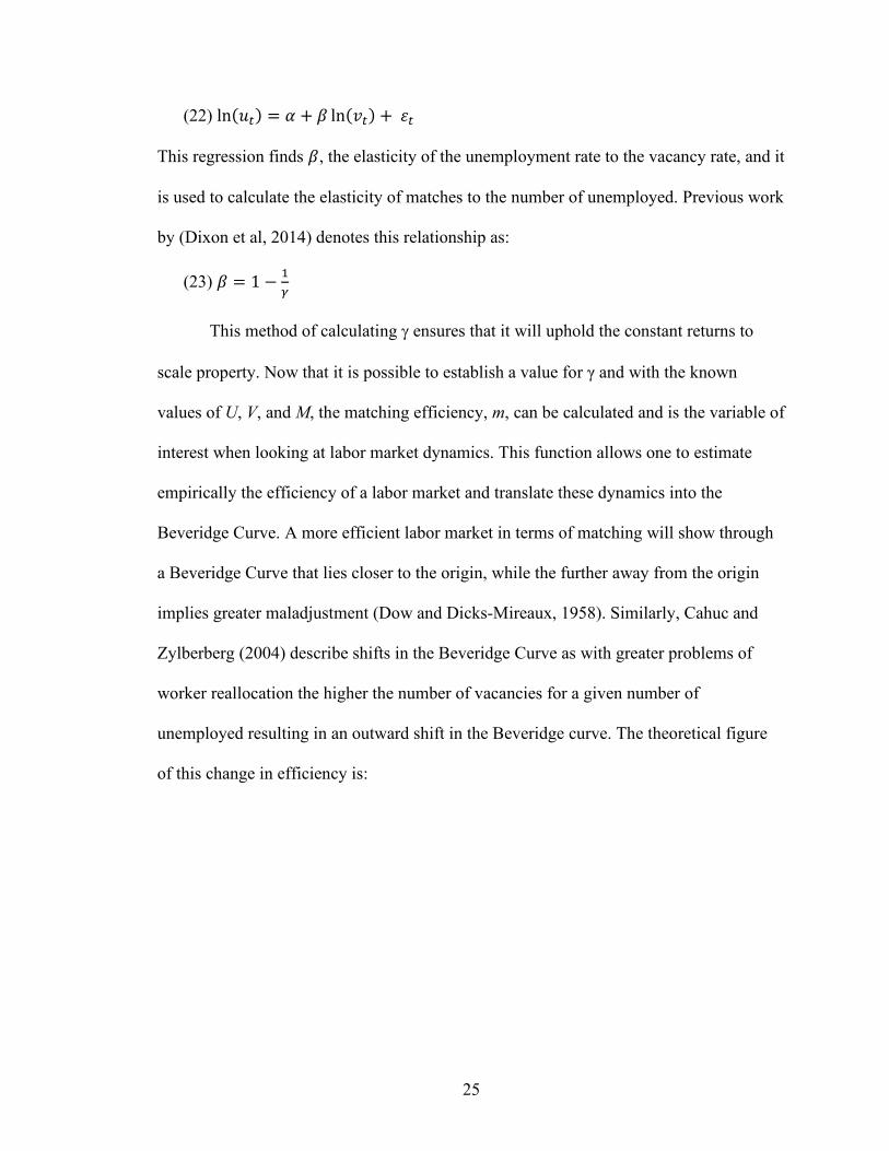
(22) ln(𝑢#) = 𝛼 + 𝛽 ln(𝑣#) +𝜀#

This regression finds 𝛽, the elasticity of the unemployment rate to the vacancy rate, and it

is used to calculate the elasticity of matches to the number of unemployed. Previous work

by (Dixon et al, 2014) denotes this relationship as:

(23) 𝛽 = 1 − >a

This method of calculating g ensures that it will uphold the constant returns to

scale property. Now that it is possible to establish a value for γ and with the known

values of U, V, and M, the matching efficiency, m, can be calculated and is the variable of

interest when looking at labor market dynamics. This function allows one to estimate

empirically the efficiency of a labor market and translate these dynamics into the

Beveridge Curve. A more efficient labor market in terms of matching will show through

a Beveridge Curve that lies closer to the origin, while the further away from the origin

implies greater maladjustment (Dow and Dicks-Mireaux, 1958). Similarly, Cahuc and

Zylberberg (2004) describe shifts in the Beveridge Curve as with greater problems of

worker reallocation the higher the number of vacancies for a given number of

unemployed resulting in an outward shift in the Beveridge curve. The theoretical figure

of this change in efficiency is:

26

Figure 8. Change in the Beveridge Curve. From Cahuc and Zylberberg (2004).

Where BC’ represents a less efficient labor market than BC; so, for a given number of

jobs vacant BC will have fewer workers unemployed than BC’.

By creating a Beveridge Curve and Matching Function for Maine and the United

States, the efficiencies of the labor markets in each region over time and the efficiencies

relative to each other can be compared using a quantitative approach.

Data

A common limitation that is faced in this research is the availability of data.

Across the literature, the measure for unemployment has been consistent and easy to find.

In terms of vacancies, up until recently it was very common for economists to make their

own indexes for a measure of vacancies due to the fact that the pool of data was either

calculated from job advertisements in limited cities or small surveys. Many others have

either gone through the Conference Board’s Help Wanted Index or the JOLTS from the

27

Bureau of Labor Statistics or combined the two. Overall, consistency is important and

recognizing the trends in the values of the data compared to one another. In early

literature, the comparison between unemployment and vacancies across regions is above

all an ordinal analysis rather than a cardinal one (Dow and Dicks-Mireaux, 1958). Data

advances have helped improve the precision of vacancies, particularly noticeable from

2005 onwards.

For the data used in this thesis, a primary source is the Bureau of Labor Statistics,

specifically their Current Population Survey (CPS) and Local Area Unemployment

Statistics (LAUS). These sources are used to obtain seasonally and non-seasonally

adjusted4 monthly unemployment and labor force data at the state and national level. The

exact values will vary between data sources as some are survey based while others

contain data reported by firms. Throughout the research close attention has been paid to

the source of each value and data consistence across each equation’s inputs has been

paramount. In terms of GDP data used throughout this thesis, the source is the Bureau of

Economic Analysis Real GDP in 2009 chained dollars.

Vacancies data was extracted using the Conference Board’s Help Wanted Index

(HWI) and extracted the monthly Total Ads from January 2006 through December 2016

for the state and national-level. The HWI is widely used in the Beveridge Curve literature

for vacancies in the United States. In past literature (Blanchard and Diamond 1989,

Abraham 1987), the vacancy data was presented as an index which then was adjusted.

However, a more accurate value is the real number of job vacancies. It is critical to have

a value of vacancies that is comparable to the value of unemployment for calculating

4 In the literature both seasonally and non-seasonally adjusted measures are used.

28

significant parameters found in the matching function. The technique used in this thesis

was the one used in Dixon et al. (2014). This author uses vacancy data in terms of

persons which are then converted to a rate by dividing by the labor force in the same way

unemployment is. Thus, both rates are comparable, and the numerators dominate the

volatility.

For new hires at the state and national level data is used from the U.S. Census

Bureau, Center for Economic Studies Quarterly Workforce Indicators. The value

extracted was the quarterly New Hires (Stable) which estimate the number of workers

who started a job that they had not held within the past year and the new hire lasted at

least a full quarter with the given employer. Jobs are counted as a stable hire in the first

quarter of employment that existed for a full quarter. For example, if a worker was hired

in the middle of the first quarter of a year, they would not be considered a stable hire until

the end of the second quarter of that year. This value was chosen to be the most accurate

representation of new hires to use in the matching function as it does not include workers

who were promoted within the same firm. Using the stable value instead of the raw value

also helps confirm that these are hires that are made with the intention of retention. There

is still a likelihood that these values are an overestimate to the actual number of new hires

per quarter. That being said they still provide a robust estimate of the actual figure for

comparison over time and at different aggregate levels, for example the state of Maine

compared to the United States.

Having new hires data limited to quarterly, the other variables were transformed

from months to quarters. While unemployment data is published quarterly, the vacancy

data is not; therefore, a transformation is made for unemployment as well as vacancy data

29

from months to quarters by doing a simple average between the three months that make

up each quarter. This ensures an additional degree of consistency between vacancies and

unemployment which is necessary as these variables are directly compared in nearly

every process of the research. For all data collected the overall time period of January

2006 thru December 2016 is used as it is available from every source. In addition, this

period encompasses an economy that experienced a severe recession, a recovery period,

and eventually the beginning of an expansion.

Table of Variables

For simplification, Table 1 presented below lists the variables primarily used in

this thesis. For each variable the name, the notation, and the source or basic calculation is

included.

Table 1. Critical Variables

Variable Name Variable Notation Source/Calculation Unemployment U Bureau of Labor Statistics Vacancies V Conference Board HWI Labor Force LF Bureau of Labor Statistics New Hires H U.S. Census Bureau Unemployment Rate u (U/LF) Vacancy Rate v (V/LF) Output/GDP GDP Bureau of Economic Analysis

30

Theoretical Beveridge Curve

As discussed in the literature review, Dow and Dicks-Mireaux (1958) present a

theoretical Beveridge Curve that highlights different levels of maladjustment as well as

periods of excess demand compared to excess supply. This figure is incredibly useful in

Beveridge Curve analysis; however, it is presented with unemployment on the vertical

axis and vacancies on the horizontal which is the opposite of how the Beveridge curve is

presented in this thesis and typically presented in literature discussing the United States’

Beveridge curve. Therefore, for simplicity, Figure 9 shows the theoretical framework of

the positioning of the Beveridge curve with vacancy rates on the vertical axis and

unemployment rates on the horizontal axis.

Figure 9. Theoretical Beveridge Curve

31

The 45º line where the unemployment rate equals the vacancy rate represents an

equilibrium condition, meaning there is an equal amount of jobs open to the number of

people looking for work. On the first Beveridge curve, 𝐵𝐶> shown in blue, (Point 2)

represents an equilibrium. For the second Beveridge curve, 𝐵𝐶^ shown in orange, (Point

4) represents an equilibrium. Although, just because both points 2 and 4 exist in

equilibrium conditions does not reflect that they are equally efficient labor market

outcomes. The further the curve is shifted out from the origin, the more structural

problems exist in theory. Thus, under this condition, 𝐵𝐶> is a healthier labor market than

𝐵𝐶^.

While shifts represent structural changes in the labor market, movements along a

Beveridge curve represent cyclical changes. During instances of high unemployment and

low vacancies there are more people looking for jobs than firms looking to hire, so there

is an excess supply of labor. 𝐵𝐶^ (Point 3) represents this scenario. During periods of

low unemployment and high vacancies there are more firms looking for workers than

workers looking for employment, therefore there is an excess demand of labor. 𝐵𝐶>

(Point 1) represents this scenario. An excess supply of labor is more likely to occur

during a recessionary period and an excess demand for labor is more likely to occur

during an expansionary period. Both an excess supply and excess demand can have

negative consequences to the efficiency of a labor market. The labor market’s degree of

sensitivity can be affected by the underlying structural problems that exist. For example,

an excess demand for labor 𝐵𝐶^ could have more of a negative impact on the efficiency

than an excess supply for labor 𝐵𝐶> due to the fact that 𝐵𝐶^ theoretically has more

structural problems than 𝐵𝐶>.

32

EMPIRICAL FINDINGS

Maine’s Beveridge Curve and Labor Market Efficiency

Maine’s Beveridge curve is shown below in Figure 10 with monthly vacancy and

unemployment rates from January 2006 through December 2016 plotted.

Figure 10. Maine Beveridge Curve

The sharp shift out from the origin and followed by movement the right on

Maine’s Beveridge curve reflects the period of the great recession. The furthermost point

to the right corresponds to the month of January 2010. After this, the Beveridge curve

begins to shift back to the left, showing a recovery process, but at a higher level of

maladjustment signaling a weaker labor market as discussed in the literature (Dow and

0.00%

1.00%

2.00%

3.00%

4.00%

5.00%

6.00%

0.00% 1.00% 2.00% 3.00% 4.00% 5.00% 6.00% 7.00% 8.00% 9.00%

Vac

ancy

Rat

e

Unemployment Rate

Maine Beveridge Curve January 2006 - December 2016

2006

2016

2009

33

Dicks-Mireaux, 1958) and the theoretical Beveridge curve created for this thesis shown

in figure 9.

In order to develop further understanding of the position of the Beveridge curve,

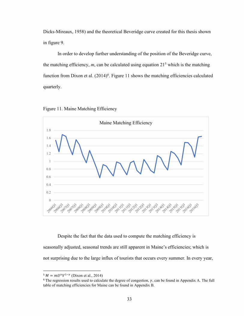
the matching efficiency, m, can be calculated using equation 215 which is the matching

function from Dixon et al. (2014)6. Figure 11 shows the matching efficiencies calculated

quarterly.

Figure 11. Maine Matching Efficiency

Despite the fact that the data used to compute the matching efficiency is

seasonally adjusted, seasonal trends are still apparent in Maine’s efficiencies; which is

not surprising due to the large influx of tourists that occurs every summer. In every year,

5 𝑀 = 𝑚𝑈a𝑉>?a (Dixon et al., 2014) 6 The regression results used to calculate the degree of congestion, 𝛾, can be found in Appendix A. The full table of matching efficiencies for Maine can be found in Appendix B.

0

0.2

0.4

0.6

0.8

1

1.2

1.4

1.6

1.8

2006

Q1

2006

Q3

2007

Q1

2007

Q3

2008

Q1

2008

Q3

2009

Q1

2009

Q3

2010

Q1

2010

Q3

2011

Q1

2011

Q3

2012

Q1

2012

Q3

2013

Q1

2013

Q3

2014

Q1

2014

Q3

2015

Q1

2015

Q3

2016

Q1

2016

Q3

Maine Matching Efficiency

34

the second quarter is consistently the quarter with the lowest efficiencies annually, and

the third quarter the highest. Beyond the seasonal effects that remain, there is also a clear

decline and recovery period cause be the recession observed with the matching

efficiency.

The efficiency drops 53.6% from the second quarter of 2006 to the second quarter

of 2009. In terms of annual averages, compared to 2006 the 2009, 2010, 2011, and 2012

matching efficiencies were 47.5%, 46.2%, 44.2%, and 44.3% lower respectively. The

2016 matching efficiency, while much healthier than the years before, is still lower than

the 2006 average. This analysis shows how the labor market in Maine has been slow to

recovery from the recession. Despite unemployment levels being around 4%, the

Beveridge curve remained shifted out for many years suggesting structural problems in

the labor market.

For a clearer understanding, figure 12 plots the Beveridge curve for Maine and

highlights the matching efficiencies that correspond with critical changes in the curve.

35

Figure 12. Maine Beveridge Curve and Matching Efficiency

From the first quarter of 2006 the Beveridge Curve for Maine began shifting out,

signaling a labor market that was becoming less efficient. Just how inefficient the market

has become can be captured utilizing the matching efficiency calculation discussed in the

methodology. From the first quarter of 2006 to the second quarter of 2009 the efficiency

has decreased by 62.33%. This movement to the right would suggest a labor market

experiencing a significant excess in labor supply. By looking at the matching efficiencies

as the curve moves to the right, this is exactly the story that is being told. The furthermost

point to the right lines up with the lowest matching efficiency that Maine experienced in

the time observed; 0.582 in the second quarter of 2009. After this point, the recovery

from the recession can be observed in the leftward movement of Maine’s Beveridge

Curve, but the fact that the curve is still shifted out compared to where it started in 2006

0.00%

1.00%

2.00%

3.00%

4.00%

5.00%

6.00%

0.00% 1.00% 2.00% 3.00% 4.00% 5.00% 6.00% 7.00% 8.00% 9.00%

Vac

anci

es

Unemployment

Maine Beveridge Curve and Matching Efficiency

2Q 2009

2Q 2008

3Q 2016

3Q 2014

1Q 2006

Change: -37.41%

Change: -39.81%

Change: 115.8%

Change: 29.78%

36

shows a relatively less efficient labor market. More recent data points to an improvement

of efficiency. Looking at the final quarter of 2015, the Beveridge Curve began to shift

back inward, with the matching efficiency increasing by 16% in 2016 alone

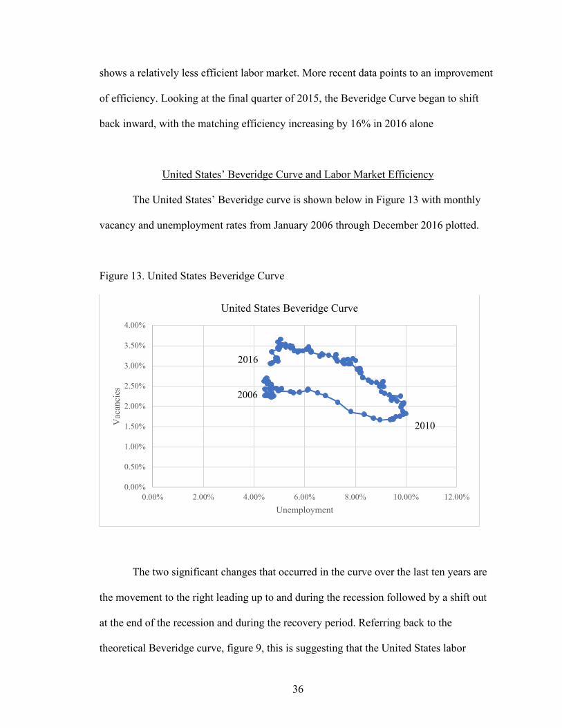
United States’ Beveridge Curve and Labor Market Efficiency

The United States’ Beveridge curve is shown below in Figure 13 with monthly

vacancy and unemployment rates from January 2006 through December 2016 plotted.

Figure 13. United States Beveridge Curve

The two significant changes that occurred in the curve over the last ten years are

the movement to the right leading up to and during the recession followed by a shift out

at the end of the recession and during the recovery period. Referring back to the

theoretical Beveridge curve, figure 9, this is suggesting that the United States labor

0.00%

0.50%

1.00%

1.50%

2.00%

2.50%

3.00%

3.50%

4.00%

0.00% 2.00% 4.00% 6.00% 8.00% 10.00% 12.00%

Vac

anci

es

Unemployment

United States Beveridge Curve

2016

2006

2010

37

market experienced a time of excess supply of labor along with potential structural issues.

These findings agree with those of Abraham (2015) and Sahin et al. (2013) as discussed

in the Literature Review; both argue that a structural problem that could be occurring is

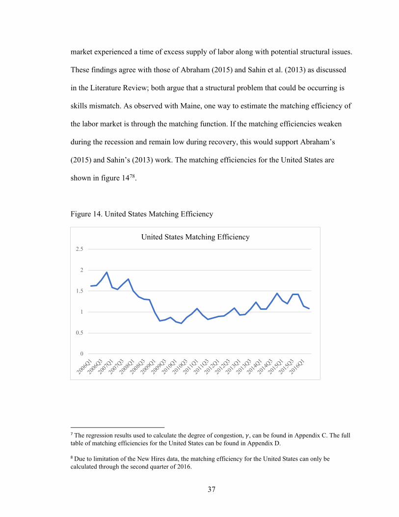
skills mismatch. As observed with Maine, one way to estimate the matching efficiency of

the labor market is through the matching function. If the matching efficiencies weaken

during the recession and remain low during recovery, this would support Abraham’s

(2015) and Sahin’s (2013) work. The matching efficiencies for the United States are

shown in figure 1478.

Figure 14. United States Matching Efficiency

7 The regression results used to calculate the degree of congestion, 𝛾, can be found in Appendix C. The full table of matching efficiencies for the United States can be found in Appendix D. 8 Due to limitation of the New Hires data, the matching efficiency for the United States can only be calculated through the second quarter of 2016.

0

0.5

1

1.5

2

2.5

2006

Q1

2006

Q3

2007

Q1

2007

Q3

2008

Q1

2008

Q3

2009

Q1

2009

Q3

2010

Q1

2010

Q3

2011

Q1

2011

Q3

2012

Q1

2012

Q3

2013

Q1

2013

Q3

2014

Q1

2014

Q3

2015

Q1

2015

Q3

2016

Q1

United States Matching Efficiency

38

The United States does not have the same seasonal changes in the efficiencies as

Maine does, but the large decline in efficiency due to the recession is present. The lowest

matching efficiency for the United States occurred in the first quarter of 2010 and was a

52.4% decline from the first quarter of 2006. The true problem that is unfolding for the

United States is that the labor market is not recovering in terms of efficiency, causing the

Beveridge curve to remain shifted out despite lower unemployment figures. Also, even

though the efficiencies appear to be rising again, the average for the first two quarters of

2016 is only 34% better than the annual average in 2009 and is 36% worse than the 2006

annual average. A question that arises from this trend is whether or not the slow recovery

is simply slow recovery, or if it is a transformation into a new normal for the labor

market. Plotting the Beveridge curve and highlighting the matching efficiency during

critical changes allows for a summarized interpretation of what is going on and is shown

in figure 15.

39

Figure 15. United States Beveridge Curve and Matching Efficiency

For the most part, the matching efficiencies related to movements in the

Beveridge curve follow the theory. In times of excess supply when the Beveridge curve

moves to the right, the efficiency is lower. As the curve moves back to the left, efficiency

rises again but because it has shifted out from the recession showing potential structural

issues, the matching efficiency is less than before. However, there is some discrepancy at

the end. In 2015 and 2016 the United States’ Beveridge Curve shifted back down, which

would correspond with a more efficient labor market, but instead the matching efficiency

decreased by 23.56%. Although, regardless of any inward movement, the Beveridge

Curve in 2015 and 2016 is still considerably shifted out compared to prior to the

recession and this fact is clear in the matching efficiencies.

0.00%

0.50%

1.00%

1.50%

2.00%

2.50%

3.00%

3.50%

4.00%

0.00% 2.00% 4.00% 6.00% 8.00% 10.00% 12.00%

Vac

anci

es

Unemployment

United States Beveridge Curve and Matching Efficiency

Q2 2010Q4 2006

Q2 2016

Q3 2015

Change: 95.06%

Change: -62.73%

Change: -23.56%

40

A Case Study on Output and the Labor Market Efficiency: A VectorAutoRegression

To observe whether output, measured in this case as Real GDP, and the matching

efficiency have a direct effect on one another, a Vector Autoregressive Model was

utilized for one and two period lags. It is important to note some of the data in this model

differs from the data used previously. The method of calculating the efficiencies

remained the same but the data for new hires and vacancies was taken from JOLTS, the

Job Openings and Labor Turnover Survey. Due to the fact that it spans over a longer time

period, 2001-2017, another recessionary period is captured. A limitation of the data its

geographical availability. Currently JOLTS is only available at a national level, therefore

for the purposes of this case study the focus will just be on the US economy.

The VAR model with two variables and two lags is presented in equations 24 and

25 below.

(24) 𝑥# = 𝛼' + 𝛼>𝑥#?> + 𝛼^𝑥#?^ + 𝛼_𝑦#?> + 𝛼z𝑦#?^ + 𝜖>#

(25)𝑦# = 𝛽' + β>𝑥#?> + β^𝑥#?^ + β_𝑦#?> + βz𝑦#?^ + 𝜖^#

The variable corresponding with the matching efficiency is 𝑥#. The actual value used for

𝑥# is the difference between the matching efficiency, which exists between 0 and 1, and

1. Essentially, the closeness to perfectly efficient. The variable corresponding with output

is 𝑦#. GDP is measured in billions of chained 2009 dollars and extracted from the Bureau

of Economic Analysis. A second difference of GDP was taken for stationarity purposes.

The important results from the VAR are shown in Table 2.

41

Table 2. VAR Results from Stata

oneminusmatch Coef. Std. Err. z P>z [95%Conf Interval] oneminusmatch L1. 1.02341 0.1222832 8.37 0 0.783739 1.26308 L2. -0.140960 0.1195177 -1.18 0.238 -0.375211 0.093289

seconddifgdp L1. 0.000126 0.0000772 1.63 0.103 -0.000025 0.000277 L2. 0.000123 0.0000749 1.65 0.099 -0.000023 0.000270

_cons 0.041242 0.0193222 2.13 0.033 0.003372 0.079113

The statistically significant result is that if the matching efficiency becomes one

standard deviation closer to fully efficient, where 𝑚 = 1, then this creates a $123 million

increase in output. Therefore, the hypothesis that the labor market efficiency influences

output is correct. To have a better visual of this relationship, figure 16 shows the impulse

response function. Given this is an unrestricted VAR, a cholesky decomposition is relied

on to construct the impulse response function.

Figure 16. Impulse Response Function from Stata

42

DISCUSSION OF FINDINGS

Direct Comparison and Contrast of the Beveridge Curve and Matching Efficiency for Maine and the United States

Throughout the analysis thus far, Maine and the United States have been observed

separately. The Beveridge Curve and Matching Function have been used as a way to

analyze labor market dynamics; and, now that the dynamics of Maine and the dynamics

of the United States are better understood, the comparison between the two can be made

to tell an even deeper story. It is important to note that Maine is aggregated into the

United States and that the trends that are occurring in Maine impact the United States;

even if the impact is very small.

Figure 17 shows the Beveridge Curve of the United States (blue) and Maine

(green) overlaid on one another.

43

Figure 17. The Beveridge Curve.

The first major difference between the two is the fact that Maine’s Beveridge

Curve shifted out significantly before the recession; which, according to Beveridge Curve

theory, shows a structural problem that the United States as a whole did not experience.

But, both Maine’s and the United States’ Beveridge Curve moved to the right during the

recession, representing excess labor supply as shown in Figure 9. This matches theory as

during recessions unemployment is high and firms are less willing to hire, resulting in an

excess supply of labor in the market.

In terms of recovery, Maine and the United States follow a similar pattern of a

movement back toward the left; however, a deviation occurs in 2015 where Maine’s

curve begins to shift back toward the origin, showing signs of a strengthening labor

market while the United States stays shifted out on a curve that theoretically shows the

0.00%

1.00%

2.00%

3.00%

4.00%

5.00%

6.00%

0.00% 2.00% 4.00% 6.00% 8.00% 10.00% 12.00%

Vac

ancy

Rat

e

Unemployment Rate

The Beveridge CurveComparison of Maine and the United States January 2006 -

December 2016

USA Maine

Jan 2006

Dec 2016

Jan 2010

44

structural problems that were potentially created from the recession. It is also interesting

to look at the slope and positioning of the Beveridge curves relative to each other.

Maine’s curve is steeper and further to the left, meaning that overall Maine experiences

periods of high vacancies and excess demand for labor. Whereas the United States’ curve

has a flatter slope, possibly indicating that higher unemployment and excess supply is

more of a problem for the labor market. Looking at the nature of these labor markets, this

dynamic makes sense. The United States is much bigger, therefore as a whole there are

an abundance of workers that the firms can choose from, making the selection easier for

the firm and creating a more difficult process for the worker; especially around the time

of a recession. For Maine, a small state with an aging population and a large amount of

out migration, the pool of workers for firms to choose from is limited. There are often

circumstances where the worker that fits the job description simply doesn’t exist in the

boundaries of the state; and, if there are not enough incentives for a worker to relocate to

where the job is, the position will remain vacant.

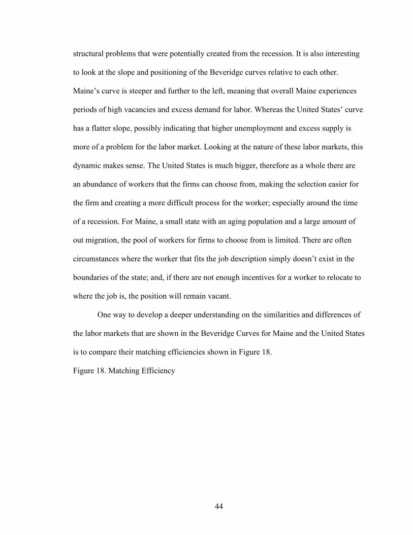
One way to develop a deeper understanding on the similarities and differences of

the labor markets that are shown in the Beveridge Curves for Maine and the United States

is to compare their matching efficiencies shown in Figure 18.

Figure 18. Matching Efficiency

45

According to the matching efficiencies, before the recession the United States’

labor market was much more efficient than Maine’s; theoretically implying that Maine

was undergoing more structural inefficiencies in their labor market, corresponding with

the sharp shift out in the Beveridge Curve. Both efficiencies experienced a dramatic drop

as a result of the recession, but what is interesting is that throughout the recovery process

the efficiencies remained relatively the same between the two regions. What is shocking

is that one might assume that the United States would have a better recovery in the labor

market due to the size and nature of the economy, but the Matching Function and the

Beveridge Curve show that this is not necessarily the case. In fact, Maine’s matching

efficiency was higher than the United States’ every third quarter after 2009. As discussed

in the Findings section, Maine’s matching efficiency has a much more seasonal trend

than the United States. This makes sense looking at the nature of Maine’s economy as it

is highly impacted by the summer tourist season.

0.25

0.45

0.65

0.85

1.05

1.25

1.45

1.65

1.85

2.05

2.25

2006

Q1

2006

Q3

2007

Q1

2007

Q3

2008

Q1

2008

Q3

2009

Q1

2009

Q3

2010

Q1

2010

Q3

2011

Q1

2011

Q3

2012

Q1

2012

Q3

2013

Q1

2013

Q3

2014

Q1

2014

Q3

2015

Q1

2015

Q3

2016

Q1

Mat

chin

g Ef

ficie

ncy

Matching EfficiencyComparison of Maine and the United States, Q1 2006 - Q2 2016

Maine USA

46

A critical observation that potentially has a serious impact is that since the third

quarter of 2015, Maine’s matching efficiency has been higher than the United States.

Ultimately, the results are claiming that Maine’s labor market is currently more efficient

than the United States. This could be due to multiple factors; such as labor force

participation, automation in the labor market, and the skill requirements of the jobs that

are vacant will all affect the labor market dynamics of these two regions that differ

dramatically in terms of size and structure.

Potential Causes for the Behavior of the Matching Efficiency in Maine

and the United States

One factor for why the matching efficiency in Maine exceeds the United States as

seen in figure 18 is the labor force participation. Figure 19 from the Maine Department of

Labor shows a comparison of Maine’s labor force participation rate to the United States.

Figure 19. Labor Force Participation Rate of Maine and the United States (From Maine

Department of Labor)

Both the United States and Maine experienced a significant decrease in their labor

force participation; however, it occurred at different times. The United States experienced

a steady decrease since 2006, while Maine experienced a decrease around the time of the

47

recession, then remained about the same from 2010 though the middle of 2013. After

2013, Maine’s labor force participation took a dramatic decrease and was down to the

level of the United States in 2015. This could be a potential reason why Maine’s

efficiency is higher as people were leaving the labor force, in turn making unemployment

figures lower while vacancies remained the same, pulling Maine’s labor market out of a

period of excess supply and into a period of excess demand.

Another potential reason is the differences in the advancement in technology for

Maine compared to the United States. While artificial intelligence has not taken over and

lead to the crisis of mass unemployment, there is skill-biased technical change (SBTC).

Where “automation tends to replace less-educated workers performing routine tasks

while it creates new demand for more-educated workers performing more complex

analysis or engaging in social interactions and communication” (Holzer, 2017). This

could be an up and coming issue for the labor market of the United States and present

itself in the fact that the Beveridge Curve has remained shifted out, signaling a structural

change, and the matching efficiency has not increased significantly throughout the

recovery process. Maine, on the other hand, is likely not experiencing this to the same

degree and thus the labor market is not affected structurally by automation, yet.

Supporting this assumption, a 2017 study published in Forbes9 ranked Maine as the 10th

least innovative state which does not signal that Maine has a healthy economy overall,

despite a seemingly healthier labor market.

9 Bloom, L. B. (2017, October 03). The 10 Most (And 10 Least) Innovative States In The U.S. Retrieved March 30, 2018, from https://www.forbes.com/sites/laurabegleybloom/2017/03/28/the-10-most-and-10-least-innovative-states-in-the-u-s/#a14998910a64

48

A classic argument for the advancement of technology is the increase of

productivity, thus the increase of the change in GDP. Looking at the changes in GDP for

Maine and the United States over the last ten years as shown in Figure 20 will also

provide insight into whether or not this higher level of matching efficiency is occurring

simultaneously with a higher change in GDP over time.

Figure 20. Percent Change in Annual Real GDP10 for Maine and the United States

It is difficult to get a solid understanding of the output trend in Maine using

quarterly changes in GDP, therefore Figure 20 uses annual changes in real GDP. What is

interesting here is that the United States faced a larger percent decrease in GDP than

Maine in 2009 but had positive changes throughout the recovery process whereas Maine

faced three consecutive years where GDP declined during recovery. Also, Maine’s

10 Annual Real GDP data is obtained from the

-3

-2

-1

0

1

2

3

2006 2008 2010 2012 2014 2016

Perc

ent C

hang

e in

GD

P

Time

Percent Change in Annual Real GDP

Maine

United States

49

percent change in GDP was slightly above the United States from 2015 to 2016, lining up

with the time where Maine’s matching efficiency exceeded the United States’ as well.

To fully understand whether or not Maine’s matching efficiency was a cause for

the increased change in GDP there would have to be more econometric analysis.

However, the fact that Maine had three years of negative change while the United States

was positive does go along with the technological advancement story. Maine may have a

healthier labor market now but in terms of output growth, they have been behind for

almost all of the observations. So, the question arises whether or not Maine is falsely

efficient because they have filled jobs with lower contributions to output and are having a

more difficult time filling positions with high skill requirements. If this is the case, it will

become a problem because if Maine has little to no innovation because they will become

less and less of a competitor in the economy relative to other states.

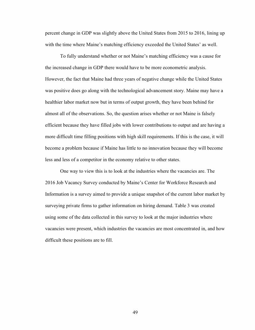
One way to view this is to look at the industries where the vacancies are. The

2016 Job Vacancy Survey conducted by Maine’s Center for Workforce Research and

Information is a survey aimed to provide a unique snapshot of the current labor market by

surveying private firms to gather information on hiring demand. Table 3 was created

using some of the data collected in this survey to look at the major industries where

vacancies were present, which industries the vacancies are most concentrated in, and how

difficult these positions are to fill.

50

Table 3. Vacancies by Industry in Maine (Modified from Maine Center for Workforce

Research)

The results from this survey are rather alarming. Nearly 36% of all vacancies in

the state of Maine are in Healthcare and Social Assistance. Not only is that a large

percentage, but it also is an industry where there appears to be a shortage of workers

because 78% of firms find it difficult to fill these vacancies. In this industry, registered

nurses appear to be most in demand with an average of 505 job openings per year based

on Maine’s 2024 Job Outlook report. In fact, registered nurses are highest in demand for

jobs across all sectors and they require a Bachelor’s degree or higher for education. A

Industry Vacancies Difficult to Fill* Healthcare and Social Assistance 35.74% 78% Retail Trade 16.42% 63% Accommodation and Food Services 12.14% 81% Administrative and Waste Services 9.49% 70% Manufacturing 5.76% 80% Construction 4.66% 93% Professional Scientific and Technical Services 3.24% 69% Transportation, Warehousing and Utilities 2.79% 91% Other Services 2.28% 88% Financial Services 2.08% 47% Wholesale Trade 1.49% 76% Arts, Entertainment and Recreation 1.26% 36% Private Education Services 1.01% 79% Management of Companies 0.85% 43% Information 0.75% 65% Natural Resources 0.06% 62%

*Share of vacancies with affirmative responses divided by total responses, excluding unspecified or blank fields.

51

potential reason why healthcare jobs are in such high demand is for the aging population.

Also, besides the fact that these jobs are difficult to fill, filling them will likely not

increase innovation or productivity in Maine’s economy. Therefore, while the matching

efficiency for Maine is better than the United States, it still is not signaling a healthy

labor market.

52

CONCLUSION

In conclusion, this thesis set out to understand labor market efficiency in the

United States and in Maine. Addressing the first research objective, the VAR model

results supports the contention that an increase in the matching efficiency leads to an

increase in GDP; however, a structured modelling approach could be adopted in future

research. A structural VAR would be appropriate in the future or panel models that

incorporates of all of the states.

Addressing the second research objective; the findings show that the estimated

efficiency of the labor markets of both Maine and the United States are worse post-

recovery than they were prior to the recession; especially in the case of the United States.

This was shown through the theoretical implications of the Beveridge curves shifting as

well as the estimated efficiencies remaining lower. The literature often looks to these

issues in the labor market as being a result of structural problems.

A structural problem that could exist in the United States and Maine are skill

mismatch. This occurs when the vacant jobs require different skills, specifically those

that require higher levels of training, than what is available in the pool of unemployed

workers. This skill mismatch could be amplified by other structural changes such as

automation. Also, the aging population could be a cause of inefficiencies as well as an

older labor force having more retirees per year, thus shrinking the pool of workers to

choose from. A particular policy implication of interest to increase efficiency is more

flexible immigration laws. Whether it be high or low skilled labor, increasing the size of

the pool of workers for firms to choose from could improve efficiency in places of excess

53

demand for labor; which Maine is currently experiencing quite intensely. As stated in the

Discussion of Findings, Maine’s labor market efficiency appears to have recovered much

better than the United States. But, a conflict for Maine is that the vacancies that are open

are difficult to fill. Beyond that, they are primarily in nursing and social assistance;

meaning that they will likely not increase output in the same way that filling a vacancy in

an innovative field would.

Future research on this topic will consist of empirically testing the different

structural problems that could be occurring, as well as better understanding the impact of

congestion on labor market efficiencies.

54

WORKS CITED

Abraham, K. G. (1983). Structural / Frictional vs. Deficient Demand Unemployment: Some New Evidence. American Economics Review, 73(4), 708–724.

Abraham, K. G. (2015). Is skill mismatch impeding U.S. economic recovery? Industrial

and Labor Relations Review, 68(2), 291–313. https://doi.org/10.1177/0019793914564962

Abraham, K. G., & Katz, L. F. (1984). Cyclical Unemployment: Sectoral Shifts or

Aggregate Disturbances? Journal of Political Economy, 94(3), 507–522. Abraham, K. G., & Wachter, M. (1987). Help-Wanted Advertising, Job Vacancies, and

Unemployment. Source: Brookings Papers on Economic Activity, 1987(1), 207–248. Retrieved from http://www.jstor.org/stable/2534516

Bellman, R. (1955). BOTTLENECK PROBLEMS, FUNCTIONAL EQUATIONS, AND

DYNAMIC PROGRAMMING. Econometrica, 23(1), 73–87. Retrieved from http://www.jstor.org.prxy4.ursus.maine.edu/stable/pdf/1905582.pdf?refreqid=excelsior:0cdf5fcf90139cec7a86e8dfa6ced47d

Blanchard, O. J., Diamond, P., Hall, R. E., & Yellen, J. (1989). The Beveridge Curve.

Brookings Papers on Economic Activity, 1989(1), 1–76. Blanchflower, D. G., & Oswald, A. J. (1994). The Wage Curve. Massachusetts Institute

of Technology. Bleakley, H., & Fuhrer, J. C. (1997). Shifts in the Beveridge Curve, Job Matching, and

Labor Market Dynamics. New England Economics Review, September, 3–19. Booth, A. L. (2014). Wage Determination and Imperfect Competition. Labour

Economics, 30, 53–58. https://doi.org/10.1016/j.labeco.2014.06.010 Burgess, S., & Profit, S. (2001). Externalities in the matching of workers and firms in

Britain. Labour Economics, 8(3), 313–333. https://doi.org/10.1016/S0927-5371(01)00036-7

Cahuc, P., & Zylberberg, A. (2004). Labor Economics. Cambridge, Massachusetts: MIT

Press Diamond, P. (2011). Unemployment , Vacancies , Wages †. American Economic Review,

101, 1045–1072.

55

Dixon, R., Lim, G. C., & Freebairn, J. (2014). Regional Beveridge Curves: A Latent Variable Approach. Regional Studies, 48(2), 254–269. https://doi.org/10.1080/00343404.2011.644238

Doughtery, C. (2011). Slow Growth Stirs Fears of Recession. Retrieved February 4,

2018, from https://www.wsj.com/articles/SB10001424053111904800304576475811201857064?mod=searchresults&page=1&pos=15

Dow, J. C. R., & Dicks-Mireaux, L. A. (1958). The Excess Demand for Labour. Oxford

Economic Papers, 10(1), 1–33. Elsby, M. W. L., Michaels, R., & Ratner, D. (2015). The Beveridge Curve : A Survey.

Journal of Economic Literarure, 53(3), 571–630. https://doi.org/10.1257/jel.53.3.571

Graham, G. (2015). Summit on Aging reveals economic vulnerability of Maine seniors -

Portland Press Herald. Retrieved March 20, 2018, from https://www.pressherald.com/2015/09/15/maine-summit-on-aging-tackles-issues-facing-state-as-population-ages/

Hansen, B. (1970). Excess Demand, Unemployment, Vacancies, and Wages. The

Quarterly Journal of Economics, 84(1), 1–23. Harry J. Holzer. (2017). Will robots make job training (and workers) obsolete?

Workforce development in an automating labor market. Retrieved March 30, 2018, from https://www.brookings.edu/research/will-robots-make-job-training-and-workers-obsolete-workforce-development-in-an-automating-labor-market/

Hobijn, B., & Şahin, A. (2013). Beveridge Curve Shifts across Countries since the Great

Recession. IMF Economic Review, 61(4), 566–600. https://doi.org/10.1057/imfer.2013.18

Jackman, R., & Roper, S. (1987). Structural Unemployment. Oxford Bulletin of

Economics & Statistics. Kajuth, F. (2017). A benchmark for wage growth through the lens of the Beveridge

curve. Applied Economics Letters, 25(7), 487–492. https://doi.org/10.1080/13504851.2017.1340561

Lilien, D. M. (1982). Sectoral Shifts and Cyclical Unemployment. American Economics

Association, 90(4), 777–793. Oswald, A. J. (1993). Efficient contracts are on the labour demand curve: Theory and

facts. Labour Economics, 1(1), 85–113. https://doi.org/10.1016/0927-5371(93)90007-5

56

Petrongolo, B., & Pissarides, C. A. (2001). Looking into the Black Box: A Survey of the Matching Function. Journal of Economic Literature, 39(2), 390–431. https://doi.org/10.1257/jel.39.2.390

Rogerson, R., Shimer, R., & Wright, R. (2004). Search-Theoretic Models of the Labor

Market: A Survey. Retrieved from http://www.nber.org.prxy4.ursus.maine.edu/papers/w10655.pdf

Shimer, R. (2005). The Cyclical Behavior of Equilibrium Unemployment and Vacancies.

American Economic Review, 95(1), 25–49. Valletta, R. (2005). Why has the U.S. Beveridge Curve Shifted Back? New Evidence

Using Regional Data. At Last, a Proper Recovery. (2015, February). The Economist. Retrieved from

https://www.economist.com/news/united-states/21643196-all-sorts-americans-are-feeling-more-prosperous-last-proper-recovery

57

APPENDICES

58

APPENDIX A: SOLVING FOR THE DEGREE OF CONGESTION IN MAINE

Table 1 shows the regression results of the estimation of equation 1 from Dixon et al.

(2014).

(1) ln(𝑢#) = 𝛼 + 𝛽 ln(𝑣#) +𝜀#

Table 1. OLS Regression Results from Stata: Maine

ln(u) Coef. Std. Err. t P>t [95% Conf. Interval] ln(v) -0.468638 0.073175 -6.4 0.000 -0.6134 -0.3238 _cons -4.500557 0.260595 -17.27 0.000 -5.0161 -3.9851

The parameter of interest is 𝛽 which is equal to −0.46836. Using the identity shown in

equation 2 from Dixon et al. (2014), the degree of congestion 𝛾 can be calculated.

(2) 𝛽 = 1 − >a

The result for the degree of congestion is that 𝛾 = 0.6809.

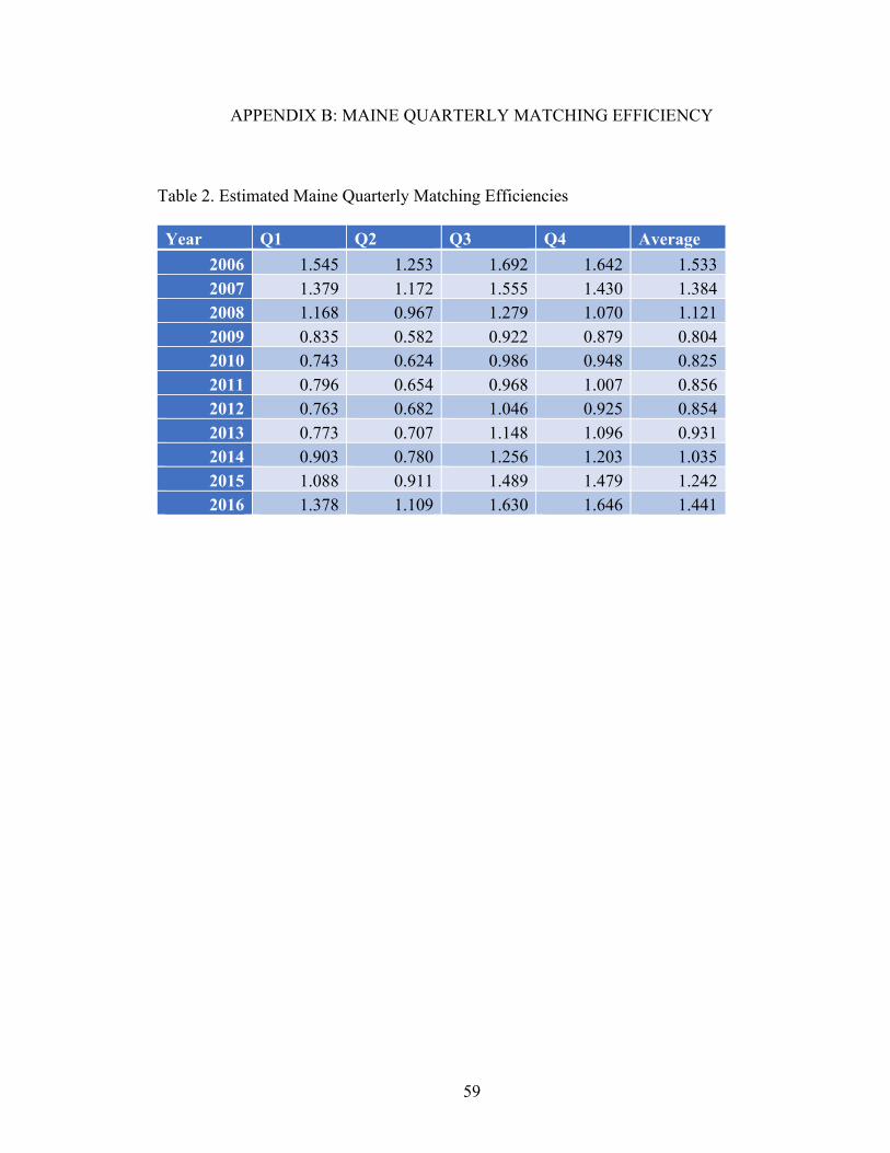
59

APPENDIX B: MAINE QUARTERLY MATCHING EFFICIENCY

Table 2. Estimated Maine Quarterly Matching Efficiencies

Year Q1 Q2 Q3 Q4 Average 2006 1.545 1.253 1.692 1.642 1.533 2007 1.379 1.172 1.555 1.430 1.384 2008 1.168 0.967 1.279 1.070 1.121 2009 0.835 0.582 0.922 0.879 0.804 2010 0.743 0.624 0.986 0.948 0.825 2011 0.796 0.654 0.968 1.007 0.856 2012 0.763 0.682 1.046 0.925 0.854 2013 0.773 0.707 1.148 1.096 0.931 2014 0.903 0.780 1.256 1.203 1.035 2015 1.088 0.911 1.489 1.479 1.242 2016 1.378 1.109 1.630 1.646 1.441

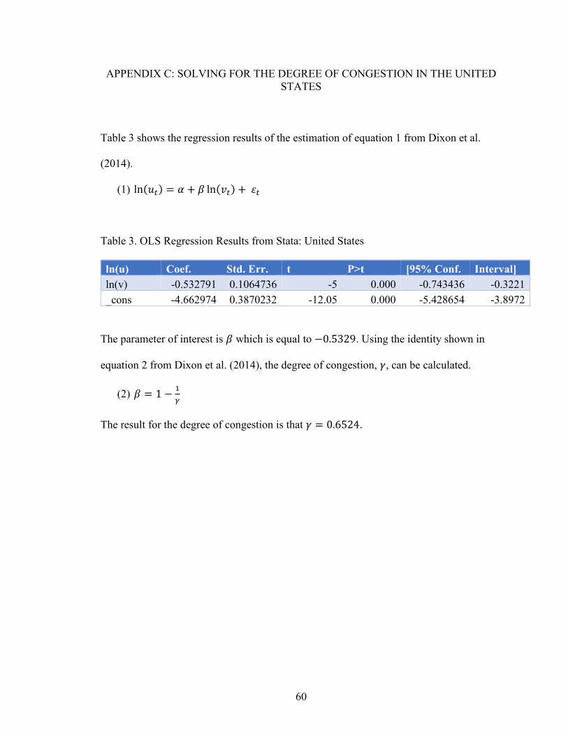
60

APPENDIX C: SOLVING FOR THE DEGREE OF CONGESTION IN THE UNITED STATES

Table 3 shows the regression results of the estimation of equation 1 from Dixon et al.

(2014).

(1) ln(𝑢#) = 𝛼 + 𝛽 ln(𝑣#) +𝜀#

Table 3. OLS Regression Results from Stata: United States

ln(u) Coef. Std. Err. t P>t [95% Conf. Interval] ln(v) -0.532791 0.1064736 -5 0.000 -0.743436 -0.3221 _cons -4.662974 0.3870232 -12.05 0.000 -5.428654 -3.8972

The parameter of interest is 𝛽 which is equal to −0.5329. Using the identity shown in

equation 2 from Dixon et al. (2014), the degree of congestion, 𝛾, can be calculated.

(2) 𝛽 = 1 − >a

The result for the degree of congestion is that 𝛾 = 0.6524.

61

APPENDIX D: UNITED STATES QUARTERLY MATCHING EFFICIENCY

Table 4. Estimated United States Quarterly Matching Efficiencies

Year Q1 Q2 Q3 Q4 Average 2006 1.625 1.635 1.760 1.956 1.744 2007 1.586 1.542 1.673 1.790 1.648 2008 1.503 1.363 1.306 1.298 1.368 2009 0.993 0.791 0.818 0.874 0.869 2010 0.773 0.729 0.872 0.957 0.833 2011 1.086 0.927 0.823 0.857 0.924 2012 0.890 0.905 0.992 1.092 0.970 2013 0.929 0.945 1.069 1.232 1.044 2014 1.077 1.076 1.243 1.451 1.212 2015 1.269 1.206 1.422 1.428 1.331 2016 1.146 1.087 * * 1.117

* Not all data used to estimate the matching efficiency is available at the U.S. Level in

Quarters 3 and 4 of 2016.

62

AUTHOR’S BIOGRAPHY

Sarah M. Welch was raised in Center Lovell, Maine and graduated from Fryeburg

Academy in 2014. In addition to her major in Financial Economics, she has a minor in

Mathematics. Throughout her time at the University of Maine she worked as both a

research assistant and a teaching assistant for the School of Economics. She is a member

of All Maine Women, a senior traditions society on campus, and SPIFFY, a student run

investment portfolio. In Spring 2016 Sarah studied abroad in San Sebastian, Spain.

Sarah is the Class of 2018 recipient of the Ryan Dana Wright Memorial Award as the top

graduating senior in the School of Economics. Upon graduation, she will remain at the

University of Maine pursuing an M.S. in Economics through an accelerated 4+1 program

and graduate in May 2019.