the analysis of large-scale turbulence characteristics in ... · through the north sangihe ridge,...
TRANSCRIPT

Ocean Sci 8 615ndash631 2012wwwocean-scinet86152012doi105194os-8-615-2012copy Author(s) 2012 CC Attribution 30 License
Ocean Science
The analysis of large-scale turbulence characteristics in theIndonesian seas derived from a regional model based on thePrinceton Ocean Model
K OrsquoDriscoll 1 and V Kamenkovich2
1Institute of Oceanography Centre for Marine and Atmospheric Sciences University of Hamburg Bundesstrasse 5320146 Hamburg Germany2Department of Marine Science The University of Southern Mississippi Stennis Space Center MS 39529 USA now at Environmental Engineering Research Centre School of Planning Architecture amp Civil EngineeringQueenrsquos University Belfast UK
Correspondence toK OrsquoDriscoll (kieranodriscollqubacuk)
Received 6 December 2011 ndash Published in Ocean Sci Discuss 16 January 2012Revised 13 July 2012 ndash Accepted 16 July 2012 ndash Published 15 August 2012
Abstract Turbulence characteristics in the Indonesian season the horizontal scale of order of 100 km were calculatedwith a regional model of the Indonesian seas circulation inthe area based on the Princeton Ocean Model (POM) As iswell known the POM incorporates the MellorndashYamada tur-bulence closure scheme The calculated characteristics aretwice the turbulence kinetic energy per unit massq2 theturbulence master scale` mixing coefficients of momen-tum KM and temperature and salinityKH etc The ana-lyzed turbulence has been generated essentially by the shearof large-scale ocean currents and by the large-scale wind tur-bulence We focused on the analysis of turbulence aroundimportant topographic features such as the Lifamatola Sillthe North Sangihe Ridge the Dewakang Sill and the Northand South Halmahera Sea Sills In general the structure ofturbulence characteristics in these regions turned out to besimilar For this reason we have carried out a detailed anal-ysis of the Lifamatola Sill region because dynamically thisregion is very important and some estimates of mixing coef-ficients in this area are available
Briefly the main results are as follows The distribution ofq2 is quite adequately reproduced by the model To the northof the Lifamatola Sill (in the Maluku Sea) and to the southof the Sill (in the Seram Sea) large values ofq2 occur inthe deep layer extending several hundred meters above thebottom The observed increase ofq2 near the very bottom is
probably due to the increase of velocity shear and the cor-responding shear production ofq2 very close to the bottomThe turbulence master scale` was found to be constant inthe main depth of the ocean while` rapidly decreases closeto the bottom as one would expect However in deep pro-files away from the sill the effect of topography results inthe` structure being unreasonably complicated as one movestowards the bottom Values of 15 to 20times 10minus4 m2 sminus1 wereobtained forKM andKH in deep water in the vicinity of theLifamatola Sill These estimates agree well with basin-scaleaveraged values of 133times 10minus4 m2 sminus1 found diagnosticallyfor KH in the deep Banda and Seram Seas (Gordon et al2003) and a value of 90times 10minus4 m2 sminus1 found diagnosticallyfor KH for the deep Banda Sea system (van Aken et al1988) The somewhat higher simulated values can be ex-plained by the presence of steep topography around the sill
1 Introduction
We investigate the distribution of turbulence characteristicswith horizontal scale on the order of 100 km in the deeplayers of the Indonesian seas calculated with a regionalmodel of the Indonesian seas circulation The model is basedon the Princeton Ocean Model (POM) incorporating theMellorndashYamada turbulence closure scheme The POM is
Published by Copernicus Publications on behalf of the European Geosciences Union
616 K OrsquoDriscoll and V Kamenkovich Large-scale turbulence characteristics in the Indonesian seas
widely used in modeling the ocean circulation in variousregions of the World Ocean (seehttpwwwaosprincetoneduWWWPUBLIChtdocspomfor POM details) POMoutput provides both dynamical (depth-integrated and 3-Dvelocities temperature salinity and sea surface height) andturbulence characteristics (kinetic energy and master scale ofturbulence mixing coefficients of momentum temperatureand salinity etc) As a rule the analysis of POM results con-cerning the 3-D circulation has been restricted to the studyof the distribution of dynamical characteristics and in a fewpapers only features of turbulence characteristics have beenintrinsically analyzed (see egEzer 2000 Oey et al 1985Cummins 2000 Wijesekera et al 2003 andEzer and Mel-lor 2004) We think that the study of such features is essen-tial to understanding the dynamics of the ocean circulationas well
We found a consistent distribution of turbulence character-istics on the scale of order of 100 km for the entire Indone-sian seas region However the interaction of the large-scaleturbulence with shear flow around basic topographic featuresin the area appears to be of primary interest To illustrate thisinteraction we first provide sections of distributions of twicethe turbulence kinetic energy (per unit mass)q2 which willbe called in what follows simply turbulence kinetic energyand the coefficient of vertical mixing of momentumKM through the North Sangihe Ridge the Dewakang Sill thesills surrounding the Halmahera Sea (specifically the northand south sills) and the Lifamatola Sill (see Fig 1 for modeldomain and section locations) In general the structure turbu-lence characteristics in these regions turned out to be similarSo we decided to focus our detailed analysis on the Lifama-tola region from the southern Maluku Sea (north of the sill)to the Seram Sea (south of the sill) because dynamically thisregion is very important and some estimates of mixing coef-ficients there are available
The Lifamatola Sill is the deepest connection between thePacific Ocean and the interior Indonesian seas the Banda Seaand the Flores Sea and is the main source of deep water tothe Seram and Banda Seas (see egGordon 2005 van Akenet al 1988 2009 andOrsquoDriscoll and Kamenkovich 2009)The deep flow across the Lifamatola Sill is one of the majorcomponents of the Indonesian Throughflow (ITF) which isa key element of the World Ocean thermohaline circulationsystem or ocean conveyor belt (see egGordon 2005 fordetails)
To the best of our knowledge there have been only a fewdirect measurements of turbulence characteristics in the In-donesian seas area We can refer to the pioneering paper ofStommel and Fedorov(1967) who discovered microstruc-ture in temperature and salinity profiles from STD recordersnear Timor and Mindanao and detailed microstructure mea-surements made byAlford et al (1999) in the Banda Seanear 100 m depth over a 2-week period Unfortunately thesedata refer to small-scale turbulence and cannot be used forthe comparison with our calculations So we can rely only
on estimates of basin-scale coefficients of vertical mixing inthe Banda and Seram Seas derived from diagnostic calcula-tions byGordon et al(2003) van Aken et al(1988) andvan Aken et al(1991) based on the 1-D temperature equa-tion suggested byMunk (1966)
To avoid confusion we would like to stress that this pa-per is not intended to analyze the internal structure of turbu-lence In this paper we analyze the characteristics of verticalturbulence provided by MellorndashYamadarsquos scheme of parame-terization It is well known that all turbulence characteristicsare chaotically pulsated both spatially and temporally Whattypes of fluid motions are responsible for these pulsationsHorizontal mixing is parameterized by Smagorinskyrsquos for-mula which takes into account sub-grid scale eddies Thespecifics of these eddies are not elaborated upon This for-mula is widely used in atmospheric and ocean modeling andis considered to be very effective We focus on the analysis ofvertical turbulent mixing in deep layers of the ocean includ-ing the bottom boundary layer The analysis is based essen-tially on the consideration of the turbulence kinetic energyequation From the standpoint of this equation we considerturbulence that is essentially generated by the shear of large-scale ocean currents and by the large-scale wind turbulenceSo our focus is on turbulence associated with basin-scalemotions in the Indonesian seas This is the main reason whywe call the analyzed turbulence large-scale turbulence Theeffect of shear is balanced by the work of buoyancy forcesdissipation of the energy vertical and horizontal diffusionand vertical and horizontal advection The contribution oflee waves into the shaping ofq2 is not considered explic-itly because they occur at a much smaller scales order of100 m The analysis of such motions usually requires a non-hydrostatic model very detailed bottom topography and hor-izontal grid spacing on the order of 10 m (see egXing andDavies 2006 2007) The effect of internal waves is recog-nized separately but parameterized in the POM very crudelyby the introduction of background mixing It is worth not-ing here that currently there are no general cirulation models(GCMs) that are able to simulate simultaneously large-scalefeatures of the circulation and such motions as small-scaleeddies filaments coming off eddies internal waves or leewaves The study of such motions is extremely importantfrom the standpoint of the internal structure of turbulencebut all known GCMs are using some kind of parameteriza-tion for such motions This does not mean that characteristicsof turbulence provided by GCMs are of no interest For ex-ample the simple Munk model based on the 1-D temperatureequation is used by many researchers to obtain an estimate ofbasin-scale turbulence mixing
We stress that mixing coefficientsKM (momentum) andKH (temperature and salinity) were not specified a prioribut calculated within the POM Because the large-scale cur-rents and temperature and salinity distributions have beenadequately described by our model we argue that the esti-mate of mixing coefficientsKM andKH is also reasonable
Ocean Sci 8 615ndash631 2012 wwwocean-scinet86152012
K OrsquoDriscoll and V Kamenkovich Large-scale turbulence characteristics in the Indonesian seas 617
Fig 1 The model domain location along with names of important topographic features and open ports The
model domain was rotated relative to lines of constant Lat - Lon so that the Indian Ocean port was located on
the JADE August 1989 CTD transect between northwestern Australia and Bali The model(xy) domain ranges
betweeni and j values of 1 to 250 respectively (seeij values along model domain edge) Model domain
corners in Lat - Lon values are as follows SW20S 118E SE13S 142E NE 11N 135E and NW
4N 111E The 4 open ports are shown as bold lines along the edge of the model domain The depth in
the grey (dotted) region is less than 100 m However the greyregion in the Indian Ocean in the southwestern
corner of the model domain is greater than 100 m but has been excluded from the model integration to facilitate
the Indian Ocean open port The red lines show locations of the sections through the North Sangihe Ridge
(1-2) the Dewakang Sill (3-4) the Lifamatola Sill (5-6) and the Halmahera Sea (7-8) discussed in Section 3
The thick black line through the Lifamatola Sill in the North-South direction shows the location of the profiles
discussed in Section 4
23
Fig 1 The model domain location along with names of important topographic features and open ports The model domain was rotatedrelative to lines of constant latndashlong so that the Indian Ocean port was located on the JADE (Java-Australia Dynamics Experiment) Au-gust 1989 CTD (conductivity temperature depth) transect between northwestern Australia and Bali The model(xy)domain ranges betweeni andj values of 1 to 250 (seeij values along model domain edge) Model domain corners in latndashlong values are as follows SW 20 S118 E SE 13 S 142 E NE 11 N 135 E and NW 4 N 111 E The 4 open ports are shown as bold lines along the edge of the modeldomain The depth in the grey (dotted) region is less than 100 m However the grey region in the Indian Ocean in the southwestern cornerof the model domain is greater than 100 m but has been excluded from the model integration to facilitate the Indian Ocean open port Thered lines show locations of the sections through the North Sangihe Ridge (1ndash2) the Dewakang Sill (3ndash4) the Lifamatola Sill (5ndash6) and theHalmahera Sea (7ndash8) discussed in Sect 3 The thick black line through the Lifamatola Sill in the northndashsouth direction shows the locationof the profiles discussed in Sect 4
Otherwise we would not obtain an adequate description ofcurrents and temperature and salinity distributions becausevalues ofKM and KH directly impact those distributionsUltimately all indirect methods of estimating mixing coef-ficients are based on the assumption of the existence of closerelationships between distributions of dynamical and mix-ing characteristics Therefore it is important to stress that allempirical constants in the MellorndashYamada scheme are fixedand do not depend on the case considered It is important tostress also that the validity of the MellorndashYamada schemehas been successfully tested for a wide variety of engineeringand geophysical flows (seeMellor and Yamada 1982) It isworth noting here that the validity of our estimate of mixingcoefficients was supported also by the comparison of themwith coefficients estimated byGordon et al(2003) andvan
Aken et al(1988) The regional model of the Indonesian seascirculation allowed us to learn a lot about the distributionof dynamical characteristics (currents temperature and salin-ity) in the region We think that our estimates of large-scaleturbulence characteristics are useful as well Unfortunatelywe have no directly measured data to support this statementHowever we also have nodirector indirectestimates againstit Our conclusion on the adequacy of estimated turbulencecharacteristics is based also on results of the analysis of theircompatibility with some general principles
We will start with a brief description of our model andbasic equations for determining turbulence characteristics(Sect 2) Then in Sect 3 we discuss results of the analy-sis of turbulence characteristics around the basic topographicfeatures mentioned above and in Sect 4 we discuss in detail
wwwocean-scinet86152012 Ocean Sci 8 615ndash631 2012
618 K OrsquoDriscoll and V Kamenkovich Large-scale turbulence characteristics in the Indonesian seas
q and ` distributions and mixing coefficientsKM and KHin the area of the Lifamatola Strait Concluding remarks areoutlined in Sect 4
2 Model description
For a full model description seeOrsquoDriscoll and Ka-menkovich (2009) The model domain Fig 1 extendsthroughout the Indonesian seas region and has 250times 250grid cells in the horizontal identified in Fig 1 byi andj The model has horizontal resolution ofsim 10 km in bothi-and j -horizontal directions which is sufficient to resolveall major topographic features in the region The ETOPO5data base was used in our calculation of smoothed topogra-phy Important localized topographic features such as sillswere smoothed following the recommendations of the POMsuch that the basic structure of the sill was retained whilethe bottom slope concerning the pressure gradient problemassociated with theσ coordinate system was not an issueThe model has four open ports to simulate the impact ofmajor currents entering and exiting the region The orthog-onal curvilinear coordinate system used in the POM hasbeen rotated relative to the latitudendashlongitude system so thatthe open port in the Indian Ocean region (IO port) lies onthe transect line extending from Java to northwest Australiaalong which observations were made (see egFieux et al1994 Sprintall et al 2000) There are three open ports in thePacific region the Mindanao Current port in the north (MCport) the New Guinea Coastal Current port (NGCC port) justto the north of New GuineaIrian Jaya and the North Equato-rial Counter Current port (NECC port) in the east (port loca-tions are shown in Fig 1) By and large Pacific waters enterthe model domain through the MC and NGCC ports and exitpartially through the NECC port Part of the Pacific watersenter the Indonesian seas area and cross through the regionbefore exiting the model domain in the Indian Ocean throughthe IO port This is the Indonesian Throughflow (ITF) Thegrey (dotted) regions in Fig 1 are shallow (depth is less than100 m) and are considered as land However the depth inthe grey region in the Indian Ocean in the southwestern cor-ner of the model domain is greater than 100 m but has beenexcluded from the model integration to facilitate the IndianOcean open port There are 29σ levels in the vertical so thatimportant features of the vertical structure of temperature andsalinity are properly resolved over all types of topography
At the open ports normal depth-averaged velocities arespecified based on the prescribed total transport and assumedsimple distributions of this velocity across the port For thenormal velocity in 3-D motion Orlanskirsquos condition withnudging was employed (seeMarchesiello et al 2001) Tan-gential velocity is zero for both the 2-D and 3-D motionPOM recommended boundary conditions are used at closedboundaries Because of various restrictions eg the NGCCcrossing the equator and the grid spacing of Levitus climatol-
ogy (Conkright et al 2002) it was not possible to calculategeostrophic velocities at the open ports from available ob-servations and climatology Therefore as an alternative weused published observations and some modeling results todetermine typical port normal velocities and total port trans-ports A detailed analysis of observational data for all portsand calculation of port normal velocities and correspondingtransports was performed It was supposed that such an ap-proach is more reliable than the use of results from a globalocean GCM
At the sea surface boundary the Adjusted SouthamptonOceanography Centre (SOC) surface flux climatology (Gristand Josey 2003) is used in the calculation of surface heatflux which is equal to the sum of long wave radiation la-tent heat (evaporation) and sensible heat fluxes Since theflux of fresh water at the surface in the Indonesian seas isvery poorly known sea surface salinity is specified from Lev-itus climatology (Conkright et al 2002) In the near surfaceand deep ocean (sub-thermocline water) a very weak nudg-ing of T andS to climatology was introduced to account formixing processes not correctly parameterized in the modelMonthly climatological winds are taken from the Compre-hensive Ocean-Atmosphere Data Set (COADS) analyzed byda Silva et al(1994) and are calculated at every internaltime step
Tides have not been directly included in the model How-ever additional friction has been incorporated into the mo-mentum equations as a proxy for important tidal frictionin the vicinity of some passages and sills The approach israther crude but tides somehow needed to be taken into ac-count Otherwise due to western intensification for exam-ple we obtained overly strong flows through certain pas-sages and straits A similar approach was taken bySchilleret al (1998) The direct incorporation of tides is a separatedifficult problem
It is generally accepted now that a background diffusivityof 10minus5 m2 sminus1 is added to the coefficients of vertical mixingto represent mixing processes not modeled by the MellorndashYamada scheme (eg internal waves) see egEzer(2000)
It was shown that the developed regional model adequatelydescribed the circulation in the Indonesian seas (OrsquoDriscolland Kamenkovich 2009 Kamenkovich et al 2009 Rosen-field et al 2010) We list principal results here First wehave shown that basic features of temperature and salinitydistributions along with the current pattern with scale of or-der of 100 km were reproduced reasonably well We demon-strated a satisfactory agreement of simulated transports withtransports observed during the INSTANT program Secondit was proved that the pressure difference between the Pa-cific and Indian Ocean is not a major factor determining thetotal transport of the ITF All factors influencing this totaltransport were revealed and their roles were clarified Thirdwe managed to disclose the path of South Pacific Water en-tering the Indonesian seas region as a branch of the NewGuinea Coastal Current We have shown that this water flows
Ocean Sci 8 615ndash631 2012 wwwocean-scinet86152012
K OrsquoDriscoll and V Kamenkovich Large-scale turbulence characteristics in the Indonesian seas 619
around Halmahera island and then enters the region throughthe Maluku Sea and across the Lifamatola Strait
The developed model uses the MellorndashYamada schemeto describe turbulence characteristics The scheme has beensuccesssfully applied to various regions of the World OceanAlthough we did not find published results of direct compar-ison of turbulence characteristics simulated by the POM (in-corporating the MellorndashYamada scheme of closure) with cor-responding observed characteristics there are many resultsof modeling such phenomena the structure of which dependssignificantly on the chosen scheme of closure For exampleEzer(2005) studying results of modeling near the DenmarkStraits bottom dense overflow came to the conclusion thatthe ldquoMellorndashYamada scheme represents the subgrid-scalemixing very wellrdquo Similarly Ezer and Weatherly(1990)studying pools of cold water flowing on the bottom of theocean in the High Energy Benthic Boundary Layer Exper-iment region in the North Atlantic concluded that bottomturbulence and boundary-layer dynamics were simulated ad-equately The POM uses Smagorinskyrsquos scheme to parame-terize sub-grid scale horizontal diffusion of momentum andscalar characteristics
For completeness of outline we write out the basic rela-tions of the MellorndashYamada turbulence closure scheme (seeMellor 2004) Coefficients of vertical mixing of momentumKM and vertical mixing of salt and temperatureKH are rep-resented by
KM = SMq` KH = SHq` (1)
We remind the reader thatq2 is twice the kinetic energy ofturbulence (per unit mass) and` is a master scale of turbu-lenceSM andSH are nondimensional characteristics depend-ing on the Richardson numberRi
Ri = minus`2
q2N2 (2)
whereN is the local buoyancy frequency For calculation ofSM andSH the following empirical formulas are used
SH =A2[1minus 6(A1B1)stf]
1minus [(3A2B2stf) + 18A1A2]Ri(3)
and
SM =A1[1minus 3C1 minus 6(A1B1)stf] + (18A2
1 + 9A1A2)Ri
1minus 9A1A2Ri (4)
Here ldquostfrdquo is a function ofRi It is introduced to describethe effect of stratification
stf(Ri) =
10 Ri ge 010minus 09(RiRic)
32 Ric lt Ri lt 001 Ri le Ric
(5)
Also A1 = 092 B1 = 166 A2 = 074 B2 = 101 andC1 = 008Ric is the critical value ofRi andRic = minus60
Two equations are formulated to determineq2 andq2` in
xyandσ coordinatesσ =z minus η
H + η whereH is the depth of
the ocean andη is sea surface height Theq2 equation is
partq2D
partt+
partuq2D
partx+
partvq2D
party+
partωq2
partσ
=part
partσ
Kq
D
partq2
partσ+
2KM
D
[(partu
partσ
)2
+
(partv
partσ
)2]
minus2DKHN2minus
2Dq3
B1lstf+
part
partx
(HAH
partq2
partx
)
+part
party
(HAH
partq2
party
) (6)
whereu andv are zonal and meridional velocities respec-tively ω is the ldquoverticalrdquo velocity in the POM (essentiallyit is the difference between the particle velocity normal tothe surfaceσ = const and the velocity with which the surfaceσ = const is moving)D = H+η Kq is the coefficient of ver-tical diffusion ofq2 whereKq = 041KH andAH = 02AM whereAM is the coefficient of horizontal diffusion of mo-mentum calculated from Smagorinskyrsquos formula The firstterm on the right-hand side (RHS) of Eq (6) is the verticaldiffusion the second term is the production of turbulence ki-netic energy (TKE) due to vertical shear the third term is thework (per unit time) of buoyancy forces the fourth term isthe dissipation of TKE and the fifth term is the horizontaldiffusion ofq2
It is useful to write out the difference form of Eq (6) Firstwe integrate this equation over the grid cell with areaSg andreplace these integrals withSg multiplied by the integrandtaken at the center of the cell The superscriptn denotes thevalue of characteristic at time momenttn = n1 where1t isthe time step Dividing all terms of the equation onSgD
(n+1)
yields(q2)(n+1)
minusD(nminus1)
D(n+1)
(q2)(nminus1)
21t+
1
D(n+1)Sg
([sum of horizontal advective fluxes
of q2minus D
]+
partωq2
partσSg
)(n)
=1
(D(n+1))2
part
partσK(n)q
(partq2
partσ
)(n+1)+
2K(n)M
(D(n+1))2
[(partu
partσ
)2
+
(partv
partσ
)2](n)
minus2K(n)H N2(n)
minus2q(nminus1)
B1l(nminus1)stf(n)(q2)(n+1)
+
1
D(n+1)Sg
(sum of horizontal diffusion fluxes ofq2)(nminus1) (7)
The q2 equation is used in many turbulence clo-sure schemes by invoking different parameterizations of
wwwocean-scinet86152012 Ocean Sci 8 615ndash631 2012
620 K OrsquoDriscoll and V Kamenkovich Large-scale turbulence characteristics in the Indonesian seas
diffusion production and dissipation of turbulence energyThe q2` equation is utilized in the MellorndashYamada schemeonly (see a discussion inBurchard 2001) This equation isas follows
partq2`D
partt
partuq2`D
partx+
partvq2`D
party+
partωq2`
partσ
=part
partσ
Kq
D
partq2`
partσ+ E1`
KM
D
[(partu
partσ
)2
+
(partv
partσ
)2]
minusE1 minus D`KHN2minus
Dq3
B1Wstf+
part
partx
(HAH
partq2`
partx
)
+part
party
(HAH
partq2`
party
) (8)
where E1 = 18 E2 = 133 andW is the so-called wallproximity function
W = 1+ E2
[`
κ(|z minus η|
minus1+ |z + H |
minus1)
]2
(9)
whereκ is von Karmanrsquos constant The physical meaningof the separate terms on the RHS of Eq (8) is the same asthe corresponding terms of Eq (6) The difference form ofEq (8) is as follows(q2`
)(n+1)minus
D(nminus1)
D(n+1)
(q2`
)(nminus1)
21t+
1
D(n+1)Sg
([sum of horizontal advective
fluxes ofq2`D]+
partωq2`
partσSg
)(n)
=
1
(D(n+1))2
part
partσ
K(n)q
(partq2`
partσ
)(n+1)+ E1`
(n)
K(n)M
(D(n+1))2
[(partu
partσ
)2
+
(partv
partσ
)2](n)
minus
E1`(n)K
(n)H N2(n)
minusq(nminus1)
B1`(nminus1)W (n)stf(n)(q2`)(n+1)
+
1
D(n+1)Sg
(sum of horizontal diffusion
fluxes ofq2`)(nminus1)
(10)
The vertical boundary conditions forq2 andq2` at the sur-face are respectively
q2= B
231
radic(τx
ρ0
)2
+
(τy
ρ0
)2
q2` = 0 at z = 0 (11)
whereτx andτy are the components of the wind stress andρ0 is the mean density The corresponding boundary condi-
tions at the bottom are
q2= B
231 C2
z (u2+ v2) q2` = 0 at z = minusH (12)
whereCz is the so-called drag coefficient calculated in themodel by using the so-called law of the wall The horizontalboundary conditions are
q2= ε q2` = ε at horizontal boundaries (13)
whereε has been set to 10minus10 The SI international system isused for dimensions of all variables considered
3 Analysis of turbulence characteristics around basictopographic features
The results are taken from the 1 August during the SouthEastern Monsoon (SEM) after 15 yr of model integration
By and large very large values of turbulence kinetic en-ergy q2 and coefficients of vertical mixingKM and KHare found in deep water around topographic features such assills in the upper mixed layer and in the vicinity of strongcurrents in the thermoclineq2 and mixing coefficients re-duce to POM background values in the interior of the oceanaway from topographic features The turbulence kinetic en-ergyq2 basically determines mixing coefficients especiallyin the interior of the ocean where the length scale` is almostconstant Values ofq2 and mixing coefficients are greatestadjacent to the sills but patterns are complicated and per-haps noisy Maximum values ofq2 aresim 10minus3ndash10minus2 m2 sminus2Values are large especially along sloping topography andthese large values can extend for significant distances inboth upstream and downstream directions In the interior ofthe ocean away from topographic featuresq2 is reducedto less than 10minus8 m2 sminus2 Maximum values ofKM andKHare sim 10minus1ndash5times 10minus1 m2 sminus1 at the sills and along slopingtopography and can be as large assim 5times 10minus4 m2 sminus1 forsignificant distances downstream and upstream of the sillsIn the thermoclineq2 and coefficients of vertical turbulentmixing are generally small but increase noticeably wherecurrents are known to be strong with maximum values ofq2
sim 5times 10minus3 m2 sminus2 andKM sim 10minus2 m2 sminus1 In the uppermixed layer (UML) large values ofq2 and coefficients ofvertical turbulent mixing are generally confined to the up-per 50 m with maximum values ofq2
sim 10minus3 m2 sminus2 andKMandKH sim 10minus2 m2 sminus1 The scale is generally small in theboundary layers and large and almost constant in the interior(on the order of 100 m)
Figure 1 shows the locations of sections presented for dis-cussion The results of estimation are shown in Figs 2 to5 We focus on 4 important passages through complex to-pography the sill through the North Sangihe Ridge the De-wakang Sill the Lifamatola Sill and the Halmahera Sea Val-ues ofq2 andKM are given for each section The full setof results includingKH ` SM andSH have been given inOrsquoDriscoll (2007)
Ocean Sci 8 615ndash631 2012 wwwocean-scinet86152012
K OrsquoDriscoll and V Kamenkovich Large-scale turbulence characteristics in the Indonesian seas 621
Fig 2 Sections of (a)q2(m2s2) and (b)KM (m2s) through the sill in the North Sangihe Ridge Locations
of points 1 and 2 at the top of the figures are given in Figure 1
24
Fig 2 Sections of (a)q2(m2s2) and (b)KM (m2s) through the sill in the North Sangihe Ridge Locations
of points 1 and 2 at the top of the figures are given in Figure 1
24
Fig 2 Sections of(a) q2(m2 sminus2) and (b) KM (m2 sminus1) throughthe sill in the North Sangihe Ridge Locations of points 1 and 2 atthe top of the figures are given in Fig 1
Fig 3 Sections of (a)q2(m2s2) and (b)KM (m2s) through the Dewakang Sill Locations of points 3 and 4
at the top of the figures are given in Figure 1
25
Fig 3 Sections of (a)q2(m2s2) and (b)KM (m2s) through the Dewakang Sill Locations of points 3 and 4
at the top of the figures are given in Figure 1
25
Fig 3 Sections of(a)q2(m2 sminus2) and(b) KM (m2 sminus1) through theDewakang Sill Locations of points 3 and 4 at the top of the figuresare given in Fig 1
Through the sill in the North Sangihe Ridge and down-stream into the Sulawesi Sea values ofq2 in the vicin-ity of bottom topography aresim 10minus3 m2 sminus2 or greater(Fig 2a) The entire Karakelong Basin below the depth ofthe Sangihe Ridge to the west and the Karakelong Ridgeto the east showsq2 greater than 2times 10minus4 m2 sminus2 Mov-ing away from topography values ofq2 generally greaterthan 2times10minus4 m2 sminus2 extend 150ndash200 km downstream of theNorth Sangihe Ridge and into the Sulawesi Basin Upstreamof the Karakelong Ridge in the Pacific Oceanq2 generally
Fig 4 Sections of (a)q2(m2s2) and (b)KM (m2s) through the Lifamatola Sill Locations of points 5 and 6
at the top of the figures are given in Figure 1
26
Fig 4 Sections of (a)q2(m2s2) and (b)KM (m2s) through the Lifamatola Sill Locations of points 5 and 6
at the top of the figures are given in Figure 1
26
Fig 4 Sections of(a)q2(m2 sminus2) and(b) KM (m2 sminus1) through theLifamatola Sill Locations of points 5 and 6 at the top of the figuresare given in Fig 1
Fig 5 Sections of (a)q2(m2s2) and (b)KM (m2s) across the Halmahera Sea Locations of points 7 and 8
at the top of the figures are given in Figure 1
27
Fig 5 Sections of (a)q2(m2s2) and (b)KM (m2s) across the Halmahera Sea Locations of points 7 and 8
at the top of the figures are given in Figure 1
27
Fig 5 Sections of(a) q2(m2 sminus2) and(b) KM (m2 sminus1) across theHalmahera Sea Locations of points 7 and 8 at the top of the figuresare given in Fig 1
becomes small within 100 km of the sloping topography Inthe thermocline abovesim 1000 m values of 10minus8 m2 sminus2 orless are seen except around the Karakelong Basin and Ridgewhere maximum values ofsim 2times 10minus3 m2 sminus2 are found inthe upper 300 m In the upper mixed layer (UML) values ofsim 2times 10minus4 m2 sminus2 are confined to the upper 50 m
The spatial pattern inKM (Fig 2b) andKH (not shown)is very similar toq2 Near sloping topography values ofKM are sim 10minus2 m2 sminus1 and often increase to 10minus1 to 5times
10minus1 m2 sminus1 at the downstream slopeKM values aresim 5times
wwwocean-scinet86152012 Ocean Sci 8 615ndash631 2012
622 K OrsquoDriscoll and V Kamenkovich Large-scale turbulence characteristics in the Indonesian seas
10minus3ndash10minus1 m2 sminus1 in the Karakelong Basin Moving awayfrom topography values ofKM sim 5times 10minus4 m2 sminus1 are seendownstream of the North Sangihe Sill into the Sulawesi Seadecreasing to the POM background value of 2times10minus5 m2 sminus1
200 km downstreamKM is small in the thermocline exceptnear the Karakelong Basin and Ridge where values reach10minus2 m2 sminus1 between 200 and 300 m
Through the Dewakang Sillq2 values of 10minus4 m2 sminus2
or greater are seen in the vicinity of the sill (Fig 3a)These values extend to 200 m above the sill increasing to5times 10minus3 m2 sminus2 or more along the passage between the silland the Flores Sea Values are generally small along slopingtopography Higher values ofq2 extend through the watercolumn over the Dewakang Sill Away from topography val-ues are reduced tosim 10minus8 m2 sminus2 Values in the UML aresim 5times 10minus4 m2 sminus2
The pattern inKM andKH (not shown) is very similar toq2 Maximum values ofKM aresim 5times 10minus3 to 10minus2 m2 sminus1
downstream of the sill into the Flores Sea (Fig 3b) Diffusiv-ities are not very large along the upstream and downstreamslopes and rapidly decrease to background values
The section through the Lifamatola Passage (Fig 4) ex-tends from the South Maluku Sea (Batjan Basin) acrossthe Seram Sea into the North Banda Sea In deep waterdownslope and downstream of the Lifamatola Sillq2 val-ues ofsim 5times 10minus5 m2 sminus2 are seen (Fig 4a) These valuesextend through the Seram Sea and into the North BandaSea reaching 5times 10minus4 m2 sminus2 in patches Upstream in theMaluku Sea large values are seen on the slope and valuesof q2 gt 5times10minus5 m2 sminus2 are seen over a substantial area nearthe bottom of the basin Values are small above sill depth Inthe UML q2 is sim 10minus3 m2 sminus2
The pattern in bothKM andKH (not shown) is similar toq2 KM values of 5times 10minus2 m2 sminus1 (Fig 4b) extend immedi-ately downstream of the Lifamatola Sill to the North BandaSea with values as high as 10minus1 m2 sminus1 seen in patchesLarge values are also seen in the Maluku Sea upstream ofthe sill Values are small above sill depth In the UML valuesreach 10minus2 m2 sminus1
The Halmahera Sea section extends from the PacificOcean to the Seram Sea The largest values ofq2 of sim
5times 10minus3 m2 sminus2ndash10minus2 m2 sminus2 are seen at the North Halma-hera Sill in the upper 200 m and generally extend acrossthe Halmahera Sea to the southern sill where values areslightly less (Fig 5b) Below sill depthq2 is sim 10minus4 m2 sminus2
or more throughout the Halmahera Basin Downstream ofthe south sill along the slope in the Seram Sea values aresim 10minus5 m2 sminus2 or greater and can reach 5times 10minus4 m2 sminus2Large values are also seen on the upstream slope in the Pa-cific Ocean Away from topographyq2 is generally small Inthe UML q2 is sim 10minus3 m2 sminus2
Patterns inKM andKH (not shown) are very similar toq2KM is largest in the Halmahera Basin where values aresim 5times
10minus3 to 10minus1 m2 sminus1 or more (Fig 5b) In the upper 200 mKM is sim 5times 10minus3ndash10minus2 m2 sminus1 at the Northern Halmahera
Fig 6 (a) u-velocities inms at the section through the sill in the North Sangihe Ridge from east (right) to
west (left) see Figs 1 and 2 for location (b)v-velocities inms at the section through the Lifamatola Passage
(at i= 138) from north (South Maluku Sea leftj= 154) to south (Seram Sea rightj= 146) see Fig 1 forij
coordinates and section location (thick black line) The five vertical lines in (b) show the locations of profiles
presented and discussed in Section 4 of the paper The distance referred to on the abscissa is essentially the
distance across the sill from the Maluku Sea in the north to the Seram Sea in the south The actual sill is located
at the shallowest point in the section(sim 70 km)
28
Fig 6 (a) u velocities in m sminus1 at the section through the sill inthe North Sangihe Ridge from east (right) to west (left) see Figs 1and 2 for location(b) v velocities in m sminus1 at the section throughthe Lifamatola Passage (ati = 138) from north (South Maluku Sealeft j = 154) to south (Seram Sea rightj = 146) see Fig 1 forijcoordinates and section location (thick black line) The five verticallines in (b) show the locations of profiles presented and discussedin Sect 4 of the paper The distance referred to on the abscissa isessentially the distance across the sill from the Maluku Sea in thenorth to the Seram Sea in the south The actual sill is located at theshallowest point in the section(sim 70 km)
Sill andsim 10minus3 m2 sminus1 at the Southern Halmahera SillKMis generally greater than 5times 10minus4 m2 sminus1 along the down-stream slopeKM is sim 10minus3 in the upper mixed layer
Our model results show that vertically sheared flows aremainly responsible for the large values ofq2 and conse-quentlyKM This is seen at topographic features and in thethermocline in regions of known strong current Figure 6shows the shear flows seen around the North Sangihe Ridgeand Lifamatola Strait areas At the sill in the North SangiheRidge the strongly sheared flow accounts for the turbulenceat the sill (Fig 6a) and causes this water to mix with warmerwater above it thereby setting up a baroclinic pressure gradi-ent and ensuring the continued overflow across the sill Thevelocity shear along the downstream slope allows water toenter the deep Sulawesi Sea Thus the relatively warm wa-ter of the deep Sulawesi basin as observed byGordon et al(2003)A similar set of processes occurs at the LifamatilaSill allowing relatively warm water to penetrate the deeperSeram Sea (Fig 6b)OrsquoDriscoll and Kamenkovich(2009)found that a very steep temperature gradient exists in
Ocean Sci 8 615ndash631 2012 wwwocean-scinet86152012
K OrsquoDriscoll and V Kamenkovich Large-scale turbulence characteristics in the Indonesian seas 623
minus01 0 01 02 03 04 05
1200
1400
1600
1800
2000
2200
2400
2600
v
de
pth
(m
)
i=138 j=154
i=138 j=152
i=138 j=150
i=138 j=148
i=138 j=146
Fig 7 Profiles of v-component of velocity [ms] at the section through the Lifamatola Passage (i=138) from
north (j=154 left) to south (j=146 right) thick black line in Fig 1 Profiles are offset for clarity for j=154
offset is 00 ms for j=152 offset is 01 ms for j=150 offset is 02 ms for j=148 offset is 03 ms for j=146
offset is 04 ms See Fig 1 for ij coordinates and Fig 6b for profile locations Vertical and horizontal lines are
shown for convenience
29
Fig 7 Profiles ofv component of velocity [m sminus1] at the sectionthrough the Lifamatola Passage (i = 138) from north (j = 154 left)to south (j = 146 right) represented as a thick black line in Fig 1Profiles are offset for clarity forj = 154 offset is 00 m sminus1 forj = 152 offset is 01 m sminus1 for j = 150 offset is 02 m sminus1 forj = 148 offset is 03 m sminus1 for j = 146 offset is 04 m sminus1 See Fig1 for i andj coordinates and Fig 6b for profile locations Verticaland horizontal lines are shown for convenience
the downstrean direction across the Lifamatola SillPolzinet al (1996) observed similar processes that accompany thespreading of Antarctic Bottom Water at the Romanche frac-ture zone in the equatorial Atlantic Ocean
In the thermocline strong shear flows are found aroundthe North Sangihe Ridge region (Fig 6a) in the MindanaoCurrent These shear flows result in large values ofq2 andcoefficients of vertical turbulent mixing (Fig 2) and the sig-nature of NPW is transformed by mixing reducing the ther-moclineSmax signature while increasing the subthermoclineSmin signature of North Pacific Intermediate Water
4 Detailed analysis of turbulence characteristics aroundthe Lifamatola Sill
First consider Fig 6b again which gives a vertical sec-tion of v velocities through the Lifamatola Sill and showsa southward flow extending from below 1200 m to the bot-tom through the sill Model simulated deep water transportsacross the sill below 1200 m are in good agreement withthose given byvan Aken et al(1988) who calculated a deepsouthward transport ofsim15 Sv from a current mooring de-ployed between January and March 1985 while model deepsouthward transport was approximately 14 Sv in February(Kamenkovich et al 2009) In the same papervan Akenet al(1988) estimated an annual deep transport of the orderof 1 Sv in good agreement with the model (seeKamenkovich
et al 2009) However later onvan Aken et al(2009) cal-culated a long-term mean deep transport of 24ndash25 Sv for34 months between 2004 and 2006 from a mooring contain-ing current meters and ADCPs at the sill as part of the IN-STANT program (seeSprintall et al 2004) The authors invan Aken et al(2009) state that the reduced transport esti-mated invan Aken et al(1988) is due partly to the shorterobservation period and partly to the smaller thickness of theoverflow layer estimated from linear extrapolation So someuncertainty remains in estimating deep transport through theLifamatola Strait The simulated structure of the velocityprofile is in very good agreement with that observed byvanAken et al(1988) All models have some tuning parame-ters to make numerical values compatible with observationsTherefore we argue that the comparison of structures of thevelocity profiles is more important than that of some numer-ical values At the sill southward velocities increase withdepth to a maximum value of over 015 m sminus1 at sim 1700 mModel velocities across the sill are in good agreement withthose ofBroecker et al(1986) who found mean velocitiesof sim 20 cm sminus1 just above the sill over a 28 day period inAugustndashSeptember 1976 However they are less than thosemeasured byvan Aken et al(1988) who found mean ve-locities of 61 cm sminus1 at 60 m above the bottom in JanuaryndashMarch 1985 andvan Aken et al(2009) who found max-imum velocities of 65 cm sminus1 at sim 70 m above the bottomSimulatedv velocities are also southward below sill depthnorth and south of the sill to a depth ofsim 2400 m Veloc-ity is northward belowsim 2400 m both north and south of thesill A weak northward current is seen to extend from 1200 minto the thermocline across the entire section Note that allmodel results presented are from the 15 August after 15 yr ofmodel run
v velocity profiles through the sill below 1200 m are shownin detail in Fig 7 It is seen that the southward current atthe sill (middle (3rd) profilebull) extends from 1300 m tothe bottom and maximum velocity is seen at about 1700 mor deeper below which velocity rapidly decreases The ob-served mean profile shows southward flow across the sillat 129 clockwise from north and into the Seram Sea Thispractically coincides with they component of model flowacross the sill since the model domain is rotated anti-clockwise relative to northndashsouth see Fig 1 The profile tothe south of the sill (4th profile) is similar to that at the sillbut the southward current is deeper because of the greaterdepth and reaches a greater maximum velocity of almost020 m sminus1 just above the bottom Moving into deeper wa-ter both south and north the southward (negative) current isnot as strong as at the sill but extends to deeper than 2000 min all cases Currents are strongly northward (positive) belowsim 2400 m at the deepest profiles (1st and 5th profiles) ex-tending through the lower 200ndash300 m of the water columnNote also the rapid change of velocity (decrease in magni-tude) just above the bottom in all profiles which is due to the
wwwocean-scinet86152012 Ocean Sci 8 615ndash631 2012
624 K OrsquoDriscoll and V Kamenkovich Large-scale turbulence characteristics in the Indonesian seas
minus10 minus5 0 5
1200
1400
1600
1800
2000
2200
2400
2600
q2 (log 10)
de
pth
(m
)
i=138 j=154
i=138 j=152
i=138 j=150
i=138 j=148
i=138 j=146
Fig 8 Profiles ofq2[m2s2] twice the turbulence kinetic energy (TKE) through the Lifamatola Passage (i
= 138) from north (j = 154) to south (j= 146) Decimal logarithmic scale is used along the horizontal axis
Profiles are offset for clarity forj = 154 offset = 0 forj = 152 offset = 2 (orq2 is multiplied by102) for j
= 150 offset = 4 (orq2 is multiplied by104) for j = 148 offset = 6 (orq2 is multiplied by106) for j = 146
offset = 8 (orq2 is multiplied by108) See Fig 1 forij coordinates See Fig 6b for profile location through
sill Vertical and horizontal lines are shown for convenience
30
Fig 8 Profiles ofq2(m2 sminus2) twice the turbulence kinetic en-ergy (TKE) through the Lifamatola Passage (i = 138) from north(j = 154) to south (j = 146) Decimal logarithmic scale is used alongthe horizontal axis Profiles are offset for clarity forj = 154 off-set = 0 for j = 152 offset = 2 (orq2 is multiplied by 102) forj = 150 offset = 4 (orq2 is multiplied by 104) for j = 148 off-set = 6 (orq2 is multiplied by 106) for j = 146 offset = 8 (orq2
is multiplied by 108) See Fig 1 forij coordinates See Fig 6b forprofile location through sill Vertical and horizontal lines are shownfor convenience
bottom boundary condition used in the POM
Km
partv
partz= Cz(u
2+ v2)12v at z = minusH (14)
From Eq (14) it follows that if v(minusH) gt 0 thenpartv
partz(minusH) gt 0 (1st and 5th profiles) ifv(minusH) lt 0 then
partv
partz(minusH) lt 0 (3rd and 4th profiles) In the case of the 2nd
profilev(minusH) is close to zero This rapid change in velocityis present in the observed profile (seevan Aken et al 2009Fig 3) which suggests that the bottom boundary conditionEq (14) is quite adequate
We analyzed vertical profiles of turbulence characteristicsat five locations across the sill Profiles ofq2 are shown inFig 8 At the sill (3rd profilebull) large values ofq2 are con-fined to the very bottom of the water column above whichvalues are rapidly reduced and are set to the model back-ground value of 10minus9 m2 sminus2 A similar profile is seen to thesouth of the sill (4th profile) This feature is also seen inthe other three profiles However in addition at these threeprofiles (1st 2nd 5th) large values ofq2 extend upward forseveral hundred meters above the bottom between 1900ndash2600 m in the 1st profile (+) 1900ndash2100 m in the 2nd pro-file () and 2000ndash2500 m in the 5th profile (times) Above this
0 50 100 150 200 250
1200
1400
1600
1800
2000
2200
2400
2600
l
de
pth
(m
)
i=138 j=154
i=138 j=152
i=138 j=150
i=138 j=148
i=138 j=146
Fig 9 Turbulence length scaleℓ[m] for the five profiles considered
31
Fig 9 Turbulence length scale`[m] for the five profiles consid-ered
layerq2 are also small and are set to the model backgroundvalue The increase inq2 above the bottom (1st 2nd and5th profiles) is reasonable because the intensity of turbulenceshould first increase as one moves downwards and then de-crease at the very bottom However due to the increase ofvelocity shear at the very bottom and ensuing shear produc-tion of q2 the pronounced increase inq2 values occurs nearthe very bottom (see Table 1)
Profiles ofq2` (not shown) are very similar toq2 profiles(Fig 8) except close to the bottom boundary The analogousstructures of Eqs (7) and (10) explain this similarity whilethe difference in bottom boundary conditions Eq (12) ex-plains the additional rapid change (decrease) ofq2` near thebottom Yet the real question is whether the distribution of` that is determined by distributions ofq2 andq2` is reason-able (see Fig 9)
How areq2 andq2` generated To answer this questionwe estimated separately all terms in Eqs (7) and (10) to re-veal the leading terms (see Tables 1 and 2) It is worth not-ing that these tables are calculated only for thoseσ levelsfor which q2 andq2` are greater than 10minus9 the point be-ing that if q2 andq2` calculated from Eqs (7) and (10) areless than this value the POM replaces them with 10minus9 inthe SI system Therefore the analysis of contributions ofdifferent terms in Eqs (7) and (10) at these levels is mean-ingless Tables 1 and 2 give estimates of the separate termsin Eqs (7) and (10) at the same 5 profiles across the sillfrom the bottomσ(kb) wherekb = 29 up to a depth of 08times water column depthσ(kb minus 6) Recalling that valuesof σ range from 0 at the surface tominus1 at the ocean bot-tom we chose the followingσ valuesσ(kb minus 6) =minus080σ(kbminus5) =minus088σ(kbminus4) =minus094σ(kbminus3) =minus09922
Ocean Sci 8 615ndash631 2012 wwwocean-scinet86152012
K OrsquoDriscoll and V Kamenkovich Large-scale turbulence characteristics in the Indonesian seas 625
Table 1Near bottom values of different terms of theq2 Eq (7) at 5 points (location indices are given) across the Lifamatola Sill as followsrate of time difference (td) 3-D advection (ad) shear production (sp) work of buoyancy forces (bp) dissipation (dp) vertical diffusion (vd)and horizontal diffusion (hd) and the difference between the left-hand side and right-hand side of Eq (7) (resid) where resid = td + ad - (vd +sp + bp + dp + hd) Leading terms are indicated by bold All units in m2 sminus3
σ td ad sp bp dp vd hd resid
(a) i = 138 j = 154σ(kb minus 6) minus90endash11 29endash11 26endash13 minus18endash11 minus16endash11 25endash13 minus27endash11 minus14endash15σ(kb minus 5) minus20endash10 minus37endash12 18endash10 minus72endash11 minus31endash10 29endash12 minus11endash11 95endash16σ(kb minus 4) minus63endash10 minus36endash10 38endash10 minus32endash10 minus15endash9 minus73endash12 47endash10 minus37endash15σ(kb minus 3) 22endash10 50endash11 14endash12 minus80endash12 minus44endash16 64endash12 27endash10 67endash17σ(kb minus 2) 67endash10 minus43endash10 54endash13 minus28endash11 minus13endash15 69endash11 19endash10 minus54endash17σ(kb minus 1) 51endash10 minus38endash10 29endash8 minus34endash10 -31-e-8 18endash9 92endash11 21endash15
(b) i = 138 j = 152σ(kb minus 4) minus15endash10 24endash10 27endash11 minus11endash10 minus13endash10 minus29endash13 31endash10 minus57endash15σ(kb minus 3) minus36endash11 11endash10 14endash11 minus48endash11 minus43endash11 minus74endash13 15endash10 minus12endash14σ(kb minus 1) 18endash12 11e-10 83e-12 minus90e-11 minus68e-18 78e-11 12e-10 minus18e-13
(c) i = 138 j = 150σ(kb minus 1) 54endash9 13endash9 32endash7 minus12endash9 minus32endash7 46endash9 67endash11 minus80endash12
(d) i = 138 j = 148σ(kb minus 2) 16endash10 25endash10 21endash9 minus16endash9 minus40endash9 36endash9 31endash10 minus65endash14σ(kb minus 1) 73endash9 10endash9 15endash6 minus98endash10 minus15endash6 minus76endash10 minus16endash10 16endash13
(e) i = 138 j = 146σ(kb minus 6) 55endash11 minus94endash11 13endash13 minus52endash11 minus12endash16 51endash14 11endash11 minus56endash17σ(kb minus 5) minus20endash12 minus24endash10 12endash11 minus10endash10 minus93endash11 69endash14 minus62endash11 18endash15σ(kb minus 4) minus75endash11 61endash11 54endash10 minus18endash10 -30endash10 minus54endash13 minus79endash11 minus15endash15σ(kb minus 2) 58endash11 minus44endash10 17endash9 minus20endash10 minus20endash9 minus17endash10 25endash10 minus49endash12σ(kb minus 1) 10endash13 minus14e-1-0 21endash9 minus56endash12 minus27endash9 20endash10 27endash10 minus33endash16
σ(kb minus 2) =minus09961σ(kb minus 1) = minus09994 The relativelylarge number ofσ levels close to the bottom allows for areasonable description of a bottom boundary layer
Table 1 shows that at all 5 profiles except the 2nd shearproduction ofq2 and its dissipation are leading factors at lev-els very close to the bottom (due to increased velocity gradi-ent at these levels see Fig 7) At other levels such a balanceof terms in Eq (7) is not observed There are levels and pro-files at which any and all terms in Eq (7) can be importantNevertheless it is worth noting that the vertical diffusion ofq2 is important at one level of the 2nd 4th and 5th profilesonly while horizontal diffusion is important at more levels(especially in profiles 1 and 2) The work of buoyancy forcesis basically unimportant at profile 1 only
It is appropriate to discuss now profiles of shear production(Fig 10) the work of buoyancy forces (Fig 11) and dissipa-tion of q2 (Fig 12) For shear production we see first thatvalues increase as one moves downwards towards the bot-tom then decrease above the bottom before finally increas-ing substantially very close to the bottom (except profile 2)which is certainly due to the increase in velocity shear closeto the bottom (Fig 7) Notice that velocity shear is small atprofile 2 Note also in Fig 7 there is very little shear justabove the bottom points particularly in profiles 1 and 2 This
minus15 minus12 minus9 minus6 minus3 0
1200
1400
1600
1800
2000
2200
2400
2600
shear production (log 10)
de
pth
(m
)
i=138 j=154
i=138 j=152
i=138 j=150
i=138 j=148
i=138 j=146
Fig 10 Profiles of sp[m2s3] ie shear production ofq2 Note that profiles are offset as in Fig 8
32
Fig 10 Profiles of sp (m2 sminus3) ie shear production ofq2 Notethat profiles are offset as in Fig 8
wwwocean-scinet86152012 Ocean Sci 8 615ndash631 2012
626 K OrsquoDriscoll and V Kamenkovich Large-scale turbulence characteristics in the Indonesian seas
Table 2Same as Table 1 but forq2`
σ td ad sp bp dp vd hd resid
(a) i = 138 j = 154σ(kb minus 6) minus46endash9 36endash9 17endash11 minus12endash9 minus74endash10 11endash11 minus18endash9 minus87endash15σ(kb minus 5) -96endash9 49endash9 11endash8 minus42endash9 minus14endash8 87endash11 minus58endash10 minus17endash13σ(kb minus 4) -22endash8 minus11endash8 16endash8 minus13endash8 minus60endash8 minus27endash10 19endash8 minus89endash13σ(kb minus 1) minus58endash11 minus28endash10 12endash8 minus14endash10 minus12endash8 minus38endash10 96endash11 minus21endash11
(b) i = 138 j = 152σ(kb minus 4) -35endash9 10endash8 11endash9 minus40endash9 minus54endash9 minus14endash11 13endash8 minus17endash14σ(kb minus 3) minus32endash11 minus67endash10 19endash10 minus65endash10 minus22endash9 minus80endash13 18endash9 minus28endash12
(c) i = 138 j = 150σ(kb minus 1) 92endash10 43endash10 12endash8 minus33endash10 minus81endash8 minus29endash9 30endash11 minus16endash9
(d) i = 138 j = 148σ(kb minus 2) 21endash11 75endash10 13endash9 minus99endash10 minus15endash9 12endash9 71endash10 minus98endash12σ(kb minus 1) 15endash9 39endash10 48endash7 minus31endash10 minus45endash7 minus15endash8 minus41endash11 minus27endash11
(e) i = 138 j = 146σ(kb minus 5) 21endash9 -97endash9 54endash10 minus44endash9 minus29endash9 17endash12 minus29endash9 minus60endash14σ(kb minus 4) 20endash10 33endash9 21endash8 minus67endash9 minus11endash8 minus22endash11 minus28endash9 minus75endash14σ(kb minus 2) 14endash10 minus13endash9 45endash9 minus53endash10 minus51endash9 minus61endash10 76endash10 minus24endash10σ(kb minus 1) 11endash11 39endash10 93endash10 minus25endash12 minus18endash9 60endash10 12endash10 minus52endash12
minus12 minus11 minus10 minus9 minus8 minus7 minus6 minus5 minus4 minus3 minus2
1200
1400
1600
1800
2000
2200
2400
2600
modulus work of buoyancy forces (log 10)
de
pth
(m
)
i=138 j=154
i=138 j=152
i=138 j=150
i=138 j=148
i=138 j=146
Fig 11 Profiles of bp ie modulus of work of buoyancy forces or modulus of buoyancy production[m2s3]
Note that values of bp are always negative Profiles are offset as in Fig 8
33
Fig 11 Profiles of bp ie modulus of work of buoyancy forces ormodulus of buoyancy production (m2 sminus3) Note that values of bpare always negative Profiles are offset as in Fig 8
lack of shear combined with the little or no shear at thesedepths in theu component of velocity (not shown) explainsthe reduction in shear production here The work of buoy-ancy forces is the product of buoyancy frequencyN2 withthe mixing coefficientKH (Eq 6) Values decrease grad-ually from 1200 m down through the water column How-ever there is an increase in values of profiles 1 (between
minus20 minus18 minus16 minus14 minus12 minus10 minus8 minus6 minus4 minus2 0
1200
1400
1600
1800
2000
2200
2400
2600
dissipation (log 10)
de
pth
(m
)
i=138 j=154
i=138 j=152
i=138 j=150
i=138 j=148
i=138 j=146
Fig 12 Profiles of dp[m2s3] ie dissipation ofq2 Profiles are offset as in Fig 8
34
Fig 12 Profiles of dp (m2 sminus3) ie dissipation ofq2 Profiles areoffset as in Fig 8
2100ndash2500 m) 2 (between 1900ndash2100 m) 4 (between 1700ndash1900 m) and 5 (between 2000ndash2400 m) Values for all pro-files increase rapidly just above the bottom In the regionof gradually decreasing values buoyancy frequency also de-creases gradually (not shown) whileKH is essentially con-stant (Fig 14) The increase in the work of buoyancy forcesabove the bottom in profiles 1 2 and 5 is due to the increasein q2 and the subsequent increase inKH while the increase in
Ocean Sci 8 615ndash631 2012 wwwocean-scinet86152012
K OrsquoDriscoll and V Kamenkovich Large-scale turbulence characteristics in the Indonesian seas 627
minus6 minus4 minus2 0 2 4 6
1200
1400
1600
1800
2000
2200
2400
2600
log10
KM
de
pth
(m
)
i=138 j=154
i=138 j=152
i=138 j=150
i=138 j=148
i=138 j=146
Fig 13 Profiles of the coefficient of vertical diffusion of momentum KM [m2s] Profiles are offset as in Fig
8
35
Fig 13 Profiles of the coefficient of vertical diffusion of momen-tumKM (m2 sminus1) Profiles are offset as in Fig 8
profile 4 is due to the increase inN2 The increase in magni-tude of dissipation close to the bottom is due to the combinedeffect of increasedq2 with decreased while the increasejust above this is due to the combined effect of decreasedq2
with increased Consider now profiles of the turbulence length scale`
From a general standpoint we should expect to see constantvalues in the main depth of the ocean with a gradual de-crease as one moves toward the bottom In fact in Fig 9constant values are seen at all profiles in the main depth ofthe ocean away from the effect of bottom topography butthe structure of at profiles 1 2 and 5 is unreasonably com-plicated when one moves toward the bottom It is difficult tofind any physical arguments to explain the rapid increase of`
below the decrease seen in these profiles We can ascribe thisbehavior to the rather complicated structure ofq2` in theseprofiles provided by Eq (10) which is also difficult to ex-plain with physical arguments We think that the procedurefor calculation of suggested by the POM does not providethe adequate behavior of` within the bottom boundary layerHowever taking into account the adequate reproduction ofdynamical characteristics we argue that some inconsisten-cies in the calculation of and connected with character-istics eg the Richardson number etc do not influence thedynamic characteristics substantially
Profiles of magnitude of buoyancy frequency squaredN2
(not shown) show that values decrease slowly as we movedown below 1200 m as expected in the open ocean How-ever profile 1 shows values increasing notably between 2300and 2600 m This is due to strengthening stratification thereas shown inOrsquoDriscoll and Kamenkovich(2009) ( their Fig13 profile C and Fig 24θndashS diagram) and as previously ob-
served byvan Aken et al(1988) their Fig 7θndashS diagram)Rapid changes ofN2 close to the bottom are probably due tosome drawbacks of the POM algorithm for calculation ofN2
in the deep oceanProfiles of the modulus of the Richardson number|Ri|
(see Eq 2) (not shown) exhibit some rapid changes close tothe bottom In profiles 1 and 5 a rapid increase just abovethe bottom followed by a rapid decrease is due to the com-bination of rapidly increasing and decreasing` with rapidlydecreasing and increasingq2 respectively and is also seenin profile 2 to a lesser extent
Finally profiles of mixing coefficientsKM and KH areprovided in Figs 13 and 14 respectively (see Eq 1) Atthe very bottom = 0 due to the model bottom boundarycondition andKM andKH have model background valuesonly Above the bottomKM and KH are large for a verythin layer becauseq SM and SH are large and is non-zero Above this againKM andKH are briefly small in thetwo deepest profiles which is explained by small values ofq and SM and SH Using the diagnostic method ofMunk(1966) Gordon et al(2003) calculated a basin-scale aver-agedKH of 133times 10minus4 m2 sminus1 from deep temperature pro-files for the Banda and Seram Seas whilevan Aken et al(1988) calculated a value of 90times 10minus4 m2 sminus1 for KH forthe deep Banda Sea system We calculated values of 15 to20times 10minus4 m2 sminus1 for KM andKH for deep water in the vicin-ity of the Lifamatola Sill The somewhat higher simulatedvalues relative to diagnostic estimates can be explained bythe presence of complicated topography around the sill Weremind the reader that in the main depth of the ocean belowthe thermocline vertical mixing is small and a backgroundvalue of 10minus5 m2 sminus1 for KM andKH is generally acceptedWe can also refer to other data Based on radon profilesand deep silicate distributionBerger et al(1988) andvanBennekom(1988) respectively found mixing coefficientsas high as 2times 10minus1 m2 sminus1 in the deep Banda Sea Otherstudies support our results of large turbulence energy andcoefficients of vertical turbulent mixing around topographyThe analysis of the Faeroe Bank Channel overflow showsturbulent mixing coefficients with values of 10minus3 m2 sminus1 to10minus2 m2 sminus1 see egSaunders(1990) Duncan et al(2003)Mauritzen et al(2001) Mauritzen et al(2001) also foundthat strong mixing extends downstream at the Faeroe BankChannel overflow while mixing is more abrupt over theDenmark Strait overflow Using the MellorndashYamada turbu-lence scheme in an idealized sloping basinMellor and Wang(1996) found mixing coefficients between 5times 10minus2 m2 sminus1
and 10minus1 m2 sminus1 in a layer extending 500 m off the bottomalong sloping topography
In conclusion we would like to remind the reader thatall calculated characteristics refer to the middle of AugustModel forcing was specified such that maximum and mini-mum transports occur in August and February respectivelyHowever the analysis showed only very small seasonal vari-ations of turbulence characteristics in the deep ocean For
wwwocean-scinet86152012 Ocean Sci 8 615ndash631 2012
628 K OrsquoDriscoll and V Kamenkovich Large-scale turbulence characteristics in the Indonesian seas
minus6 minus4 minus2 0 2 4 6
1200
1400
1600
1800
2000
2200
2400
2600
log10
KH
de
pth
(m
)
i=138 j=154
i=138 j=152
i=138 j=150
i=138 j=148
i=138 j=146
Fig 14 Profiles of the coefficient of vertical diffusion of temperature or salinityKH [m2s] Profiles are offset
as in Fig 8
36
Fig 14 Profiles of the coefficient of vertical diffusion of tempera-ture and salinityKH(m2 sminus1) Profiles are offset as in Fig 8
illustration we provide Table 3 where August February andannual mean values of q2 are presented for the deep layersin the vicinity of the Lifamatola Sill Thus August valuesof turbulence characteristics are quite representative for allmonths of the year
5 Summary and concluding remarks
The distribution of large-scale turbulence characteristics inthe Indonesian seas region on the horizontal scale of order of100 km calculated with a regional model have been inves-tigated The model is based on the Princeton Ocean Model(POM) incorporating the MellorndashYamada turbulence closurescheme We stress that vertical mixing coefficientsKM (mo-mentum) andKH (temperature and salinity) were not speci-fied a priori but calculated within the POM along with twicethe turbulence kinetic energy (per unit mass)q2which wehave simply called turbulence kinetic energy master lengthscale and the Richardson number etc As has been shownin several papers the incorporation of the MellorndashYamadaclosure scheme in the POM gives a reasonable descriptionof turbulence characteristics of the same scale as dynamicalcharacteristics see for exampleEzer(2000) It is appropri-ate to stress that the MellorndashYamada scheme was success-fully tested on a wide variety of engineering and geophysicalflows (Mellor and Yamada 1982) By and large the analy-sis of POM results has generally been restricted to the dis-tribution of dynamical characteristics We think the study ofconsistent turbulence characteristics is also essential to un-derstanding the ocean dynamics
To avoid confusion we would like to stress that this pa-per is not intended to analyze the internal structure of tur-
bulence Our aim was to analyze vertical turbulent mixing indeep layers of the ocean including the bottom boundary layerprovided by the MellorndashYamada scheme of parameterizationThe analysis is based essentially on the consideration of theturbulence kinetic energy equation From the standpoint ofthis equation we consider turbulence that is generated bythe shear of large-scale ocean currents and by the large-scalewind turbulence So our focus is on turbulence associatedwith basin-scale motions in the Indonesian seas This is themain reason why we refer to the analyzed turbulence as large-scale turbulence The effect of shear is balanced by the workof buoyancy forces dissipation of the energy vertical andhorizontal diffusion and vertical and horizontal advectionThe contribution of small-scale motions (eg lee waves) intothe shaping ofq2 is not considered explicitly For exam-ple the lee waves occur at much smaller scales order of100 m The analysis of such motions usually requires a non-hydrostatic model very detailed bottom topography and hor-izontal grid spacing on the order of 10 m (see egXing andDavies 2006andXing and Davies 2007) The effect of inter-nal waves is recognized separately but parameterized in thePOM very crudely by the introduction of background mix-ing It is worth noting here that currently there are no GCMsthat are able to simulate simultaneously large-scale featuresof the circulation and such motions as small-scale eddies thefilaments coming off eddies internal waves or lee waves Thestudy of such motions is extremely important from the stand-point of the internal structure of turbulence but all knownGCMs parameterize such motions This does not mean thatcharacteristics of turbulence provided by GCMs are of no in-terest For example the simple Munk model based on the 1-Dtemperature equation is used by many researchers to obtainan estimate of basin-scale turbulence mixing
The regional model of the Indonesian seas circulation ex-tends throughout the entire Indonesian seas region Thereare 250times 250 grid cells in the horizontal with resolution ofsim 10 km and 29σ levels in the vertical All major topo-graphic features in the region are resolved The model hasfour open ports to simulate the impact of major currents en-tering and exiting the region 3 in the Pacific for the Min-danao Current New Guinea Coastal Current and North Equa-torial Counter Current and 1 in the Indian Ocean throughwhich the ITF exits the model domain POM recommendedboundary conditions are used at closed boundaries At thesurface heat flux is calculated from surface flux climatologyand wind stress is calculated from monthly climatologicalwinds
The model allowed us to learn a lot about the distribu-tion of dynamical characteristics (currents temperature andsalinity) in the Indonesian seas We think that our estimatesof large-scale turbulence characteristics are useful as wellIn addition to the comparison with diagnostic estimates ofmixing coefficients byGordon et al(2003) van Aken et al(1988) andvan Aken et al(1991) our conclusion on ade-quacy of estimated turbulence characteristics is based also
Ocean Sci 8 615ndash631 2012 wwwocean-scinet86152012
K OrsquoDriscoll and V Kamenkovich Large-scale turbulence characteristics in the Indonesian seas 629
Table 3Near bottom values ofq2 in August February and annual mean at 3 points across the Lifamatola Sill All units inm2 sminus3
j = 154 j = 150 j = 146
q2Aug q2
Feb q2Ann Mean q2
Aug q2Feb q2
Ann Mean q2Aug q2
Feb q2Ann Mean
σ(kb minus 6) 21e-5 20e-5 21e-5 11e-9 11e-9 11e-9 11e-9 11e-9 11e-9σ(kb minus 5) 31e-5 31e-5 31e-5 11e-9 11e-9 11e-9 52e-5 40e-5 46e-5σ(kb minus 4) 72e-5 74e-5 73e-5 11e-9 11e-9 11e-9 10e-4 68e-5 84e-5σ(kb minus 3) 11e-9 11e-9 11e-9 11e-9 11e-9 11e-9 11e-9 11e-9 11e-9σ(kb minus 2) 11e-9 11e-9 11e-9 11e-9 11e-9 11e-9 13e-5 17e-5 15e-5σ(kb minus 1) 24e-5 21e-5 23e-5 82e-5 10e-4 91e-5 50e-6 74e-6 62e-6
on results of the analysis of their compatibility with somegeneral principles
We found a consistent distribution of turbulence character-istics on the scale of order of 100 km for the entire Indone-sian seas region However the interaction of the large-scaleturbulence with shear flow around basic topographic featuresin the area appears to be of primary interest The analysis ofturbulence characteristics in the vicinty of basic topographicfeatures such as the North Sangihe Ridge the DewakangSill the sills surrounding the Halmahera Sea (specifically thenorth and south sills) and the Lifamatola Sill revealed verylarge values of turbulence kinetic energyq2 and coefficientsof vertical mixingKM andKH in deep water around thesetopographic featuresq2 and mixing coefficients reduce toPOM background values in the interior of the ocean awayfrom topographic features and outside the upper mixed layerand the vicinity of strong currents in the thermocline The tur-bulence kinetic energyq2 basically determines mixing coef-ficients especially in the interior of the ocean where the scale` is almost constant By and large the structure of turbulencecharacteristics in these regions turned out to be similar Be-cause of these results and since the Lifamatola Strait is veryimportant dynamcially and some estimates of mixing coef-ficients are available there we decided to focus our detailedanalysis of turbulence characteristics around the LifamatolaSill
Model simulated deep water transports across the Lifama-tola Sill are in good agreement with those estimated byvanAken et al (1988) but are somewhat less than those esti-mated byvan Aken et al(2009) Simulated velocities show asouthward flow extending from below 1200 m to the bottomthrough the sill The structure of the simulated velocity pro-file at the sill is in very good agreement with that observedby van Aken et al(2009) which shows a southward flowextending from below 1200 m to the bottom We argue thatthe comparison of structures of velocity profiles is more im-portant than that of separate values Southward velocities in-crease with depth to a maximum value of over 015 m sminus1 atsim 1700 m Model velocities across the sill are in very goodagreement with those ofBroecker et al(1986) but are lessthan those measured byvan Aken et al(1988) andvan Akenet al (2009) Note that some uncertainty remains in esti-
mating deep transport through the Lifamatola Strait Mov-ing away from the sill and into deeper waters both north andsouth these southward currents extend to a depth of almost2400 m below which strong simulated current reversals areseen in both the southern Maluku and Seram Seas A notablerapid change in velocity magnitude near the bottom due tothe POM bottom boundary condition is seen in all profiles
The distribution ofq2 is quite adequately reproduced bythe model The structure ofq2 shows that to the north ofthe Lifamatola Sill (in the Maluku Sea) and to the south ofthe Sill (in the Seram Sea) large values ofq2 occur in thedeep layer extending several hundred meters above the bot-tom Above this layerq2 values are small and are set to themodel background value This increase inq2 above the bot-tom is reasonable because the intensity of turbulence shouldfirst increase when one moves downwards and then decreaseat the very bottom The pronounced increase ofq2 near thevery bottom is probably due to the increase of velocity shearand the corresponding shear production ofq2 very close tothe bottom
Since the turbulence length scale` in the MellorndashYamadaclosure scheme is calculated from the solutions to both theq2
andq2` equations we estimated all terms in these equationsseparately to reveal the leading factors In 4 of the 5 profilesanalyzed a balance exists between shear production ofq2
and its dissipation close to the bottom due to increased ve-locity gradient Notably there areσ levels at which any andall terms can be important vertical diffusion is important atoneσ level only while horizontal diffusion is important atmore levels and the work of buoyancy forces is unimpor-tant at 1 profile only The same features are seen for theq2`
profilesShear production values increase as one moves towards
the bottom and decrease above the bottom due to a reductionin shear before increasing rapidly just above the bottom dueto increased shear The work of buoyancy force values de-crease gradually as one moves down through the water col-umn Away from the sill in deeper water increased valuesare seen for a depth of several hundred meters above the bot-tom due to an increase in the mixing coefficientKH beforedecreasing again as the bottom is approached
wwwocean-scinet86152012 Ocean Sci 8 615ndash631 2012
630 K OrsquoDriscoll and V Kamenkovich Large-scale turbulence characteristics in the Indonesian seas
For turbulence length scale` constant values are seen inthe main depth of the ocean which rapidly decrease closeto the bottom as one would expect However in deep pro-files away from the sill the effect of topography results inthe structure being unreasonably complicated as one movestowards the bottom Since it is difficult to find any physicalarguments to explain this rapid increase of` we doubt thatis reproduced near the bottom adequately by the model con-sidered Nevertheless this inconsistency does not influencethe dynamical characteristics substantially
Using the diagnostic method ofMunk (1966) Gordonet al (2003) calculated a basin-scale averaged deep waterKH of 133times 10minus4 m2 sminus1 from temperature profiles for theBanda and Seram Seas whilevan Aken et al(1988) calcu-lated a value of 90times10minus4 m2 sminus1 for KH for the deep BandaSea system We calculated values of 15 to 20times 10minus4 m2 sminus1
for KM andKH for deep water in the vicinity of the Lifam-atola Sill The somewhat higher simulated values can beexplained by the presence of steep topography around thesill We remind the reader that in the main depth of theocean below the thermocline vertical mixing is small anda background value of 10minus5 m2 sminus1 for KM andKH is gen-erally accepted We can also refer to other data that supportour results of large coefficients of vertical turbulent mixingaround topography Based on radon profiles and deep sil-icate distributionBerger et al(1988) and van Bennekom(1988) respectively found mixing coefficients as high as2times 10minus1 m2 sminus1 in the deep Banda Sea The analysis ofthe Faeroe Bank Channel overflow showed turbulence mix-ing coefficients with values of 10minus3 m2 sminus1 to 10minus2 m2 sminus1see egSaunders(1990) Duncan et al(2003) and Mau-ritzen et al(2001) Mauritzen et al(2001) also found thatstrong mixing extends downstream of the Faeroe Bank Chan-nel overflow while mixing is more abrupt over the Den-mark Strait overflow In an idealized sloping basinMel-lor and Wang(1996) found mixing coefficients between5times 10minus2 m2 sminus1 and 10minus1 m2 sminus1 along sloping topographyin a layer extending 500 m off the bottom
AcknowledgementsK OrsquoDriscoll would like to thank the NavalOceanographic Office for supporting his graduate educationV Kamenkovich gratefully acknowledges support from the Na-tional Science Foundation through grants OCE 96-33470 and OCE01-18200
Edited by A Schiller
References
Alford M Gregg M and Ilyas M Diapycnal mixing in theBanda Sea results of the first microstructure measurements inthe Indonesian throughflow Geophys Res Lett 26 2741ndash27441999
Berger G Bennekom A V and Kloosterhuis H Radon profilesin theIndonesian archipelago Neth J Sea Res 22 395ndash4021988
Broecker W S Patzert W C Toggweiler J R and StuiverM Hydrography chemistry and radioisotopes in the southeastAsian waters J Geophys Res 91 14345ndash14354 1986
Burchard H On theq2` Equation by Mellor and Yamada (1982)J Phys Oceanogr 31 1377ndash1387 2001
Conkright M E Locarnini R A Garcia H E OrsquoBrien T DBoyer T P Stephens C and Antonov J World Ocean At-las 2001 Objective Analyses Data Statistics and Figures Cd-rom documentation National Oceanographic Data Center SilverSpring MD 2002
Cummins P Stratified flow over topography time-dependent com-parisons between model solutions and observations Dynam At-mos Oceans 33 43ndash72 2000
da Silva A M Young C C and Levitus S Atlas of SurfaceMarine Data 1994 Volume 2 Anomalies of Directly ObservedQuantities NOAA Atlas NESDIS 7 US Department of Com-merce NOAA NESDIS 1994
Duncan L Bryden H L and Cunningham S A Friction andmixing in the Faroe Bank Channel outflow Oceanol Acta 26473ndash486 2003
Ezer T On the seasonal mixed layer simulated by a basin-scaleocean model and the Mellor-Yamada turbulence scheme J Geo-phys Res 105 16843ndash16855 2000
Ezer T Entrainment diapycnal mixing and transport in three-dimensional bottom gravity current simulations using the Mellor-Yamada turbulence scheme Oc Mod 9 151ndash168 2005
Ezer T and Mellor G A generalized coordinate ocean model anda comparison of the bottom boundary layer dynamics in terrain-following and z-level grids Oc Mod 6 379ndash403 2004
Ezer T and Weatherly G L A numerical study of the interactionbetween a deep cold jet and the bottom boundary layer of theocean J Phys Oceanogr 20 801ndash816 1990
Fieux M Andrie C Delecluse P Ilahude A G KartavtseffA Mantisi F Molcard R and Swallow J C Measurementswithin the Pacific-Indian oceans throughflow region Deep-SeaRes I 41 1091ndash1130 1994
Gordon A L Oceanography of the Indonesian Seas and TheirThroughflow Oceanography 18 14ndash27 2005
Gordon A L Giulivi C F and Ilahude A G Deep topographicbarriers within the Indonesian seas Deep-Sea Res II 50 2205ndash2228 2003
Grist J P and Josey S A Inverse analysis adjustment of the SOCair-sea flux climatology using ocean heat transport constraints JClimate 20 3274ndash3295 2003
Kamenkovich V M OrsquoDriscoll K T A and Nechaev D Dy-namics of the Indonesian Seas Part II ndash The role of pressurehead J Mar Res 67 159ndash184 2009
Marchesiello P McWilliams J M and Shchepetkin A Openboundary conditions for log-term integration of regional oceanicmodels Oc Mod 3 1ndash20 2001
Mauritzen C Price J Sanford T and Torres D Circulation andmixing in the Faeroese Channels Deep-Sea Res II 52 883ndash9132001
Mellor G L Users Giude for a three-dimensional primitive equa-tion numerical ocean model Tech rep Program in Atmosphericand Oceanic Sciences Princeton University 2004
Ocean Sci 8 615ndash631 2012 wwwocean-scinet86152012
K OrsquoDriscoll and V Kamenkovich Large-scale turbulence characteristics in the Indonesian seas 631
Mellor G L and Wang X Pressure Compensation and the BottomBoundary Layer J Phys Oceanogr 26 2214ndash2222 1996
Mellor G L and Yamada T Development of a turbulence clo-sure model for geophysical fluid problems Rev Geophys SpacePhys 20 851ndash875 1982
Munk W H Abyssal Recipes Deep-Sea Res 13 707ndash730 1966OrsquoDriscoll K T A A regional model of the Indonesian Seas cir-
culation Phd dissertation Department of Marine Science TheUniversity of Southern Mississippi 2007
OrsquoDriscoll K T A and Kamenkovich V M Dynamics of theIndonesian seas circulation Part I ndash The influence of bottom to-pography on temperature and salinity distributions J Mar Res67 119ndash157 2009
Oey L Y Mellor G L and Hires R I A three-dimensionalsimulation of the Hudson-Raritan estuary Part I Description ofthe model and model simulations J Phys Oceanogr 15 1676ndash1692 1985
Polzin K L Speer K G Toole J M and Schmitt R W In-tense mixing of Antarctic Bottom Water in the equatorial AtlanticOcean Nature 380 54ndash57 1996
Rosenfield D Kamenkovich V OrsquoDriscoll K and Sprintall JValidation of a regional Indonesian seas model based on a com-parison between model and INSTANT transports Dyns AtmOc 50 313ndash330 2010
Saunders P Cold outflow from the Faeroe Bank Channel J PhysOceanogr 20 29ndash43 1990
Schiller A Godfrey J S McIntosh P C Meyers G and Wijf-fels S E Seasonal Near-Surface Dynamics and Thermodynam-ics of the Indian ocean and Indonesian Throughflow in a GlobalOcean General Circulation Model J Phys Oceanogr 28 2288ndash2312 1998
Sprintall J Gordon A Molcard R Ilahude G Bray N Chere-skin T Cresswell G Feng M Ffield A Fieux M HautalaS Luick J Meyers G Potemra J Susanto D and WijffelsS The Indonesian Throughflow Past Present and Future Moni-toring Proceedings from the Sustained Observations for Climateof the Indian Ocean Workshop Perth Australia Technical re-port IOCCLIVAR 2000
Sprintall J Wijffels S Gordon A L Ffield A Molcard R Su-santo R D Soesilo I Sopaheluwakan J Surachman Y andvan Aken H INSTANT A new international array to measurethe Indonesian Throughflow Eos 85 369ndash376 2004
Stommel H and Fedorov K N Small scale structure in tempera-ture and salinity near Timor and Mindanao Tellus 19 306ndash3241967
van Aken H M Punjanan J and Saimima S Physical aspectsof the flushing of the East Indonesian basins Neth J Sea Res22 315ndash339 1988
van Aken H M Bennekom A J V Mook W G and PostmaH Application of Munkrsquos abyssal recipes to tracer distributionsin the deep waters of the southern Banda basin OceanologicaActa 14 151ndash162 1991
van Aken H M Brodjonegoro I S and Jaya I The deep-watermotion through the Lifamatola Passage and its contribution to theIndonesian throughflow Deep-Sea Res I 56 1203ndash1216 2009
van Bennekom A Deep-water transit times in the eastern Indone-sian basins calculated from dissolved silica in deep and intersti-tial waters NethJ Sea Res 22 341ndash354 1988
Wijesekera H W Allen J S and Newberger P A Modelingstudy of turbulent mixing over the continental shelf compari-son of turbulent closure schemes J Geophys Res 108 1ndash25doi1010292001JC001234 2003
Xing J and Davies A M Influence of stratification and topogra-phy upon internal wave spectra in the region of sills GeophysRes Lett 33 1ndash5doi1010292006GL028092 2006
Xing J and Davies A M On the importance of non-hydrostaticprocesses in determining tidally induced mixing in sill regionsCont Shelf Res 27 2162ndash2185 2007
wwwocean-scinet86152012 Ocean Sci 8 615ndash631 2012
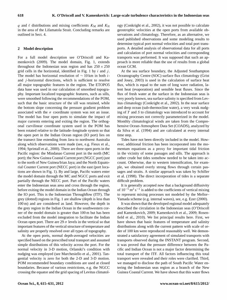
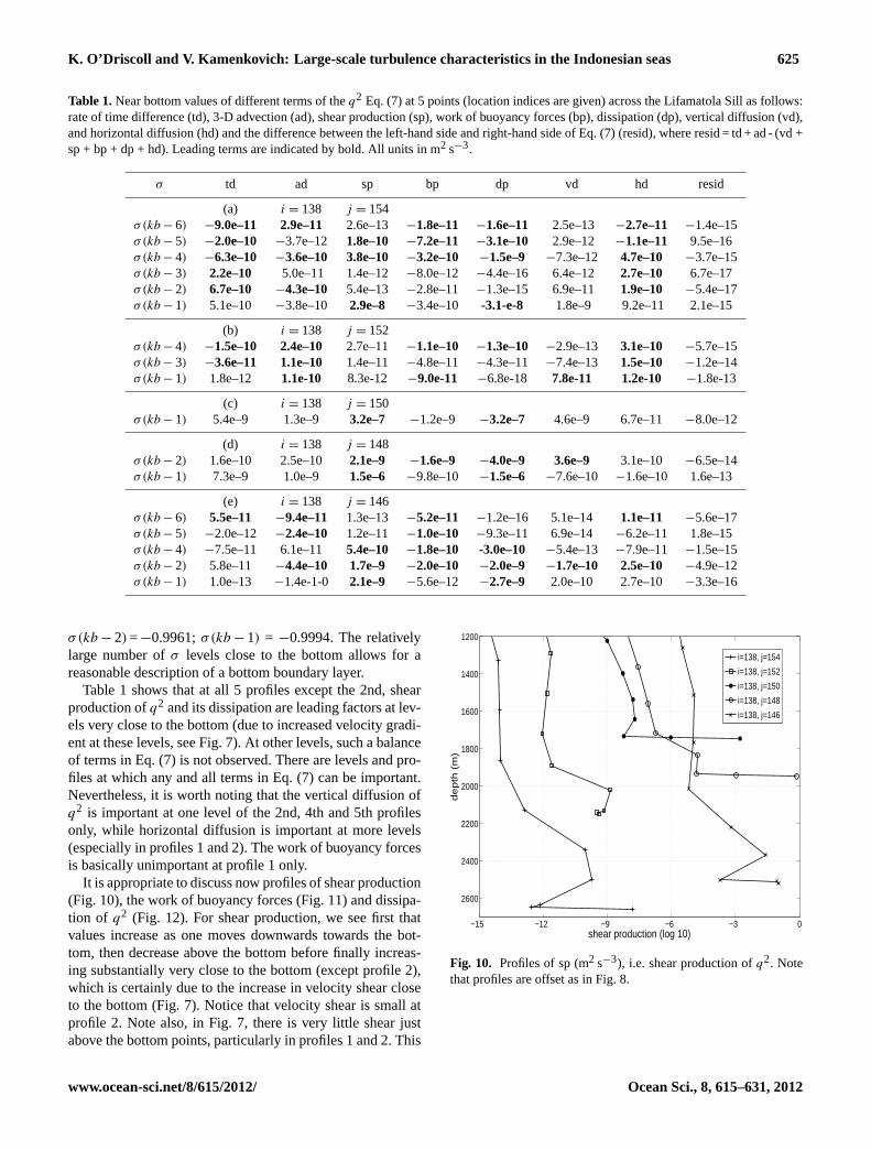
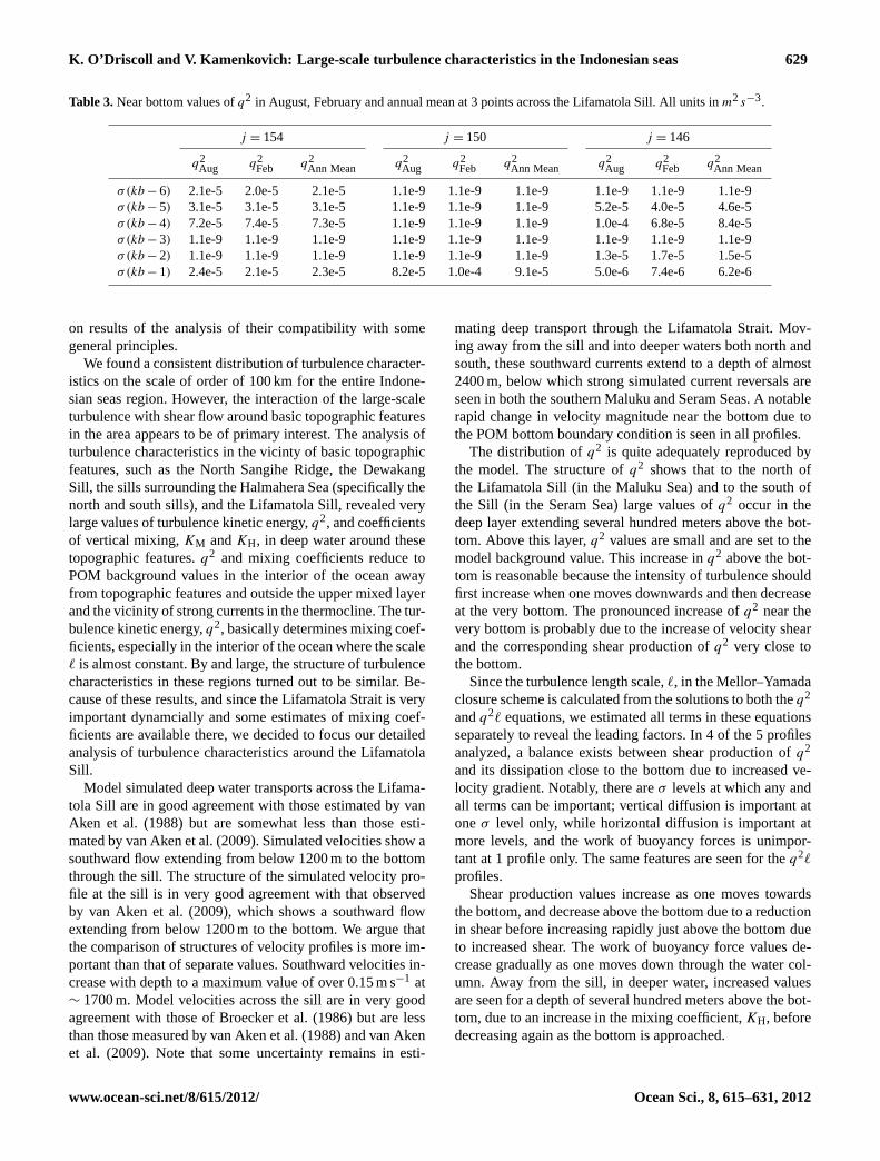