the analysis of thermal power stations and their...
TRANSCRIPT

The Analysis of Thermal Power Stations and their Interaction with the Power System
using Simulator Test Methods
Jan Andersson
Technical Report No. 294Department of Electrical Power Engineering
1996

School of Electrical and Computer Engineering
CHALMERS UNIVERSITY OF TECHNOLOGY
Göteborg, Sweden
Technical Report No. 294
ISSN 0346–718X
The Analysis of Thermal Power Stations and
their Interaction with the Power System
using Simulator Test Methods
by
Jan Andersson
Submitted to the School of Electrical and Computer Engineering,
Chalmers University of Technology,
in partial fulfilment of the requirements for the degree of
Doctor of Philosophy
Department of Electric Power Engineering,
Division of Electrical Power Systems
Göteborg, September 1996
GOTEBORG
CH
AL
ME
RSTEKNISKAHOG
SKO
LA

CHALMERS TEKNISKA HÖGSKOLA
Institutionen för Elkraftteknik, avdelningen för Elkraftsystem
S–412 96 GÖTEBORG, Sweden
ISBN 91–7197–388-5
Chalmers Bibliotek
ReproService
Göteborg, november 1996
To Elvie, Carleen andmy parents.

List of abbreviations and symbols
BFK load shedding (In Swedish BelastningsFrånKoppling)
BTK load reconnection (In Swedish: BelastningsTillKoppling)
DUBA automatic restoration equipment (In Swedish: DriftUppByggnad-sAutomatik)
EBK power shedding (In Swedish: EffektBortKoppling)
EHV Extra High Voltage
HV High Voltage
HVDC High Voltage Direct Current
hrs. hours
PID Proportional Integrating Derivative
PSS/E Power System Simulator for Engineering
ROBO rotating disconnection of load (In Swedish: ROterande BOrt- koppling)
SVC Static Var Compensator
α
firing angle [degrees]
α
s
steady state active load voltage dependence
α
t
transient active load voltage dependence
γ
extinction angle [degrees]
∆
f stationary frequency fault [Hz]
∆
P active power peak [pu]
∆
P mismatch between mechanical and electrical power [MW]
∆
P
0
connected single load at nominal frequency [MW]
∆
P
G
increase of generator production [MW]
∆
P
L
load decrease due to frequency decrease [MW]
τ
1
,
τ
2
time constants for cooling down of a house [hours]
ω
angular velocity [rad/s]
ω
0
pre-disturbance angular velocity [rad/s]

A, B constants associated with the cooling down of a house
a
0
, a
1
, a
2
parameters for the load frequency dependence
Ep0-Ep3’ operating modes of the hydro turbine governor
f system frequency [Hz]
f
0
reference value of system frequency [Hz]
H
n
unit inertia [s]
I
d
dc current [kA]
J
n
moment of inertia [kgm
2
]
k load frequency dependence [pu/Hz]
k
1
load frequency dependency in the system [MW/Hz]
L
c
commutation inductance [H]
L
d
inductance at the dc side of a HVDC station [H]
L
s
short circuit inductance [H]
L
t
transformer inductance [H]
n
p
exponential load frequency dependency
P proportional regulation [pu]
P active power consumption [MW, pu]
P
tot
total system load [MW]
P
0
total load before load connection [MW]
P
0
active power consumption at pre-fault voltage [pu]
P
r
active power recovery [pu]
Q reactive power production [MVAr]
R permanent droop [pu]
S total static gain [MW/Hz]
S
G
static gain from the generators [MW/Hz]
S
L
”static gain” from the load [MW/Hz]
S
n
rated generator power [MVA]
S
s
short circuit power [MVA]

T
G
servo time constant [s]
T
i
inside house temperature [°C]
T
i0
pre-outage inside house temperature [°C]
T
o
outside temperature [°C]
T
pr
active load recovery time constant [s]
T
r
integrating time constant [s]
U
1
, U
2
line voltage at the feeding and the receiving end [pu]
U
di
dc voltage over the line [kV]
U phase to phase voltage [kV]
u commutation angle [degrees]
V supplying voltage [pu]
V
0
pre-fault value of the supplying voltage [pu]
W
k
kinetic energy [MWs]
Y
ekv
, Z
ekv
parameters for the line equivalent circuit [
Ω
/phase]
X
L
, X
π
parameters for the simplified line equivalent circuit [
Ω
/phase]
X
s
series capacitor [
Ω
/phase]

Abstract
This thesis describes a new method of testing power stations withregard to their frequency control behaviour and analyses resultsobtained using this new method.
The test concept is based on that the power station unit to be testedremains synchronized onto its normal strong network, whereas the fre-quency control behaviour is set up to be that of the conditions if theunit was working on a much smaller network, using a computer basedsimulator system and feeding simulated control signals to the input ofthe units frequency control system. For preliminary tests or for testingconditions that could be hazardous to test on a real unit, the system canalso be connected to a power station simulator simulating the unit,where such a simulator is available.
The method has been tested extensively, first on a power station simu-lator and then in field tests against three different real power stationunits at the Stenungsund power station, Stenungsund, Sweden.
Based on these tests models are developed for the turbine systems, thesteam systems, the frequency control systems and other vital systemsof a thermal power plant. It analyses how the expected response of thistype of a unit would be under different conditions,e.g. island operationand gives tools and recommendations for testing of such power plantswith this method.
A certain analysis is also done with regard to the ability of a thermalpower station of the type tested to be responsible for the frequencycontrol of a small island network, if such operation should becomenecessary. It concludes that these possibilities are perhaps better thenwhat would be generally expected. In certain cases such a thermalpower station can even outperform hydroelectric units when it comesto the ability to exercise frequency control.
This project has been a research project at the Department of ElectricPower Engineering at Chalmers University of Technology, Gothen-burg, Sweden, sponsored by the Swedish National grid authority, Sven-ska Kraftnät, before 1992 by Vattenfall. It has earlier been presented ina licentiate thesis in January 1994 [2] and in a report presented at theMEPS conference, Wroclaw, Poland in September 1996.
Keywords
: network simulator, frequency control, island operation,thermal power station, turbine model

Acknowledgements
I would like to thank my supervisor, professor Bertil Stenborg, for hisassistance throughout this project and for his interest in it, as well asfor many helpful comments.
Special thanks should also be given to Svenska Kraftnät, who throughtheir support made this project possible and especially to Mr. KennethWalve, who initiated this project and who has been very helpful andencouraging through the same.
I would also like to thank the staff and management at the Stenungsundpower station and especially the manager of operations Hugo Holm,who have been very cooperative and whose cooperation and helpful-ness have been most essential to the completion of this project.
In addition I would like to thank the staff at the Department of ElectricPower Engineering for general assistance in different ways and espe-cially professor Jaap Daalder for valuable comments.

Contents
Abstract 1
Acknowledgements 3
Contents 5
Chapter 1 Introduction 1
Chapter 2 Background and previous work within this project 5
2.1 Measurements regarding the auxiliaries. ...............................................62.2 Simulator construction and design .........................................................82.3 Software on the interface computer .....................................................102.4 Software on the supervising computer .................................................112.5 The power station interface ..................................................................132.6 Measuring system ................................................................................14
Chapter 3 Measurements and simulations at the Stenungsund power station 17
Chapter 4 Turbine system models 33
4.1 The Stenungsund power station ...........................................................344.2 Basic steam cycle models ....................................................................374.3 Steam source pressure, constant or not ................................................374.4 Steam temperature, constant or not ......................................................394.5 The intercept valves and control system ..............................................444.6 The condenser system ..........................................................................474.7 A simplified steam cycle model ...........................................................484.8 Power/steam consumed by the feedwater system ................................504.9 High pressure turbine response ............................................................564.10 Effects of the steam lines ...................................................................584.11 The control valve and the control valve limiter .................................694.12 The frequency control system ............................................................744.13 The importance of the feedback variable ...........................................794.14 Control system dead time ...................................................................82
Chapter 5 Boiler system models 85
5.1 Is there a need for a boiler model? .......................................................855.2 Manufacturers limits ............................................................................865.3 Sliding pressure operation ....................................................................875.4 A general boiler model .........................................................................88

5.5 Long term tests and models ................................................................. 91
Chapter 6 Composite models of entire power plants 93
6.1 Units in valve control mode with sufficient steam storage capacity ... 936.2 Including the feedwater system ........................................................... 966.3 Simplified models ............................................................................... 99
Chapter 7 Auxiliary systems of the power station 103
7.1 The feedwater system ........................................................................ 1037.2 Fuel system ........................................................................................ 1107.3 Combustion airflow control .............................................................. 112
Chapter 8 Island operation. Problems, prerequesites and operating recommendations 115
8.1 Moment of inertia considerations ...................................................... 1168.2 The importance of the droop value ................................................... 1178.3 Load distribution based on the speed of response ............................. 1208.4 Mixed sources of production ............................................................. 1218.5 Operating recommendations ............................................................. 125
Chapter 9 Recommended test procedures for testing power plants 127
9.1 Connecting a unit for testing ............................................................. 1279.2 Security considerations ..................................................................... 1299.3 Data needed for a test ........................................................................ 1339.4 Basic step response tests ................................................................... 1359.5 Steam storage versus boiler response test ......................................... 1369.6 Parallel operation test ........................................................................ 1379.7 Time constant test .............................................................................. 1389.8 Power System Stabilizer test ............................................................. 1389.9 Tests on a planned network ............................................................... 1399.10 Load shedding tests ......................................................................... 141
Chapter 10 Future work 143
Chapter 11 Conclusions 145
References 147
Appendix ASpecific results for the Stenungsund power station 149
Appendix B

Measurement system, detailed description 155
Appendix C The power station interface 161

Introduction
1
Chapter 1 Introduction
Many power stations are operated in a mode where their frequencycontrol systems are not active, as these units are operated with a fairlylarge governor deadband, which makes them insensitive to normal fre-quency variations and which leaves the task of frequency control toother stations on the network. However situations can well be antici-pated where it becomes a necessity to activate the frequency controlsystems of such power stations in order to maintain the security of thenetwork. In particular this will be the case if the network, intentionallyor accidentally, is subdivided into islands in such a way that the powerstations performing the normal frequency control are separated fromthose that are operated with a deadband. In such a situation the securityof the network in some such islands will depend entirely on whether ornot the power stations that normally use deadband operation are able tosuddenly have their frequency control systems put into an active modeand thus assume the responsibility for maintaining the network fre-quency.
It is easy to imagine that a need to rely on the behaviour of a systemthat has never been tested for such operation would mean a low level ofsecurity and leave much up to chance. It is therefore necessary that thebehaviour of the power stations under such circumstances can be testedand verified as part of the proper planning for emergencies that is anintegral part of network security. However such tests are difficult tomake without that the test would in itself be a threat to network secu-rity. To actually divide the network into islands and run a test would becostly and involve taking large risks.
To rely entirely on computer simulations using standard power stationmodels and industry standard simulation programs, such as PSS/E orSimpow, is not a sufficient way of testing in order to obtain a reliableforecast as to how the system will behave in island operation either.There are too many uncertain factors regarding the behaviour of thepower station units themselves and there is also the big problem thatthe
theoretical
behaviour of the power station is all that can beaccounted for. This is a considerable limitation compared to an actualfield test, which will also detect all the factors that deviate from theplanned or modelled behaviour: settings on control systems may bedifferent from what the specifications were, the systems may have adifferent behaviour due to the aging of components or similar and also

Chapter 1: Introduction
2
the way that the plant is operated by the station operators may influ-ence the result to a large extent.
It is a well known fact from power systems all over the world that ifsuch a special operating situation occurs it is quite often that the situa-tion can not be handled properly, sometimes with an outage as a directresult. A typical example was when the Danish island Zealand was dis-connected from the main nordic power grid as a result of a networkvoltage collapse in Sweden. The danish power stations suddenly had totake over the frequency control of the island network and large fre-quency and voltage swings occurred. Only through several correctiveoperator interventions could the system be made to survive. Similarly,a recent test with island operation in the Ätran valley in Swedenresulted in a blackout, as the frequency control system, that had notbeen tested for this purpose, failed to maintain stability, leading to alarge frequency drop, followed by disconnection. These are just two ofmany cases that illustrate the need for a reliable method of testing thefrequency control systems and the behaviour of entire power stationswith regard to frequency control and island operation.
Previously the only available test method has been to actually dividethe power system up so that the unit to be tested gets its own island net-work to supply. This will surely be a good test of the unit in question,as it is a 100% realistic island operation, but it also means a considera-ble calculated risk that there may be large frequency oscillations withinthat island network or in the worst case a complete blackout. Takingsuch risks in order to perform the tests in question may in some casesbe justified, but is very often completely unacceptable. A typical casewhere this can never be done is the Stenungsund power station, northof Gothenburg, Sweden. Here the local loads consist mainly of anumber of petro-chemical industries that are all very sensitive to anynetwork disturbances and that all of them suffer very high costs if theprocess is interrupted and has to be restarted again. Not only will manyhours of production be lost, in addition virtually all chemicals that arein the process have to be dumped and burned, with both high costs andimpact on the environment as well. In such a network the idea of actu-ally disconnecting from the main power grid is unrealistic and suchtests would never be accepted.
An opposite approach of just isolating the unit to be tested and letting itrun in in-house operation is not realistic either. In house load is verylow and reasonably constant and offers no realistic test environment.To build an artificial, controllable load would of course be one

Introduction
3
approach, but the cost of building such a load, capable of burning offthe full power of the generator of the power station unit to be tested,often several hundred MW, would be extremely high, in addition tothat the tests would be very expensive to perform as all the producedpower would be dumped.
What is needed is instead a method that allows for the testing of thepower station units while they remain synchronized onto the main gridbut where it is still possible to get a good tests of how they wouldbehave if they were in active frequency control mode and responsiblefor the frequency control of a limited-size island type power network.
In order to develop a safe test method a project has been conducted atChalmers University of Technology, with the support of the Swedishnational grid authority Svenska Kraftnät, up to 1992 by Vattenfall. Theproject has been aimed at developing a test method where the fre-quency control characteristics of a power station unit can be tested bythe use of a simulator while the unit remains connected to the normalnetwork, and where e.g. the behaviour of the unit during island opera-tion can be tested without any need for actually dividing up the net-work.
The project has included simulations, measurements, field tests as wellas developing and building the simulator system. It has also included alarge amount of computer software development.
This test method, where the control signal is simulated but where theunit to be tested remains synchronized onto the normal, strong networkis a new approach, that as far as is known to the author, has never beenused before anywhere in the world.
Most of the diagrams presented in this report are from tests on actualpower station units, in operation. Where tests have been made against apower station simulator it is explicitly stated.

Chapter 1: Introduction
4

Background and previous work within this project
5
Chapter 2 Background and previous work within
this project
The simulator is based on the fact that there is in most cases no inter-change of information between the power station and the network,except the information that is given by the network itself in terms of itsvoltage level and its frequency at the point of delivery. The status of thenetwork is recorded by the voltage and frequency control systems,whereas the generator itself will deliver its output in a like mannerregardless of frequency variations; at least within the frequency limitsthat can be accepted on a network in operation. There can of course besecondary effects of frequency variations due to frequency dependen-cies of the auxiliary systems of the power station, but these effects arenormally quite limited and are normally quite effectively counteractedby internal control systems. Hydro power units have few auxilliarysys-tems, but thermal power stations have several; such as the feedwatersystem, fuel system, firing fans etc.
Figure 2.1 Basic principle of the simulator system.
If the effects on the auxiliary systems due to variations in frequencycan be said to be very small, within the range of frequencies that can be
Power station
Main generator
Auxiliaries
Simulatorsystem
Variablefrequency
Normalnetwork
Fixed frequency(normal network)
Output power
G
M
Controlsystem
Output power

Chapter 2: Background and previous work within this project
6
anticipated, then a simulator can be built by using a setup as indicatedin . In this case the simulated frequency is used only to supply a signalto the control systems and we will then need just a few watts, whereasthe main generator as well as the auxiliary systems of the power stationremain connected to the normal network. In order to use this concept itis important to verify that the effects of frequency variations, at leastwithin the range of frequency variations that can be anticipated or tol-erated, onto the power station unit through the auxiliaries can beneglected. If this would not be the case this concept of a simulatorcould not be used. Therefore one of the first tasks within this projecthad to be to try to estimate the effects of reasonably sized frequencydeviations unto the auxiliary systems.
2.1 Measurements regarding the auxiliaries.
When estimating the effects onto the auxiliaries one must take intoaccount that frequency deviations during system emergencies can besubstantially beyond the size of such variations during normal undis-turbed operation. However, the goal of preparing for e.g. island opera-tion is to obtain an operation that is at least reasonably stable and thatprovides for a fairly stable network frequency. In particular unstableoperation where the frequency oscillates up and down even duringfairly constant network load must clearly be avoided. Whereas normalfrequency deviations in e.g. the Swedish national grid normally staybelow 0.1 Hz on a continuous basis, deviations in island operationcould maybe be allowed to oscillate in the range of ± 0.25 Hz or so. Ifvery large frequency oscillations, say ±1 Hz or more, were to occur ona more or less continuous basis the operation must be said to be cum-bersome and sensitive loads may experience serious disturbances. Theexact limits will have to be set for each planning case on an individualbasis, depending on the type of loads that are connected to the networkin question. In most cases a much larger deviation can be tolerated as aslow drift in frequency compared to the case where the frequencyoscillates. If the frequency drifts up or down slowly even a deviation ofa couple of Hz can be tolerated for most types of loads.
The ideal way to verify the effects of frequency change on the auxiliarysystems would have been to vary the network frequency while the sta-tion was in operation and then make measurements on the various aux-iliary systems in question. That could not be done by in-houseoperation, as then it would be impossible to separate the cause from the

Background and previous work within this project
7
effect, and to alter the main network frequency just to perform thesemeasurements is of course not feasible.
There are however natural frequency changes on the network all thetime. Most these are fairly slow and quite subtle changes that are just aresult of the normal frequency regulation and such changes are not suf-ficient when it comes to verifying he behaviour of the auxiliaries. How-ever, there are also certain changes that are of a more drastic nature.These are the result of sudden loss of a major generating unit and if theunit in question is e.g. a major nuclear generating station then theeffects are quite noticeable. They often show a frequency drop of 0.4 to0.6 Hz under a few seconds, until the networks responds to the change.
Frequency changes of this type are almost always due to the loss of anuclear generating unit. The 12 nuclear power plants that are in opera-tion in Sweden show operating statistics such that around 10 such casesper year would be typical; i.e. one case every month. By simply mak-ing measurements of all critical system parameters of a thermal powerplant in actual normal operation it would therefore be possible tosooner or later trap such an event and get recordings of the actualbehaviour of the auxiliary systems.
Measurements of this nature has been performed on units 2,3 and 4 atthe Stenungsund power plant. On a couple of occasions frequency dipsof the kind described above were observed. These involved a frequencydrop of about 0.2 Hz and no effects of significance in were observed onthe auxiliaries. A typical recording (Figure 2.2), made on unit 4 of theStenungsund power station, shows the network frequency, the genera-tor output, the combustion airflow and the total fuel flow to the burners.
In the case listed above the frequency dip was about 0.2 Hz which withan static droop of say 5%, taken as an average of the generator unitsthat perform the frequency control duties of the network at the time,would correspond to a load-change equal to about 8% of the rated out-put power of these units. That is a substantial change and more thanwhat could be expected in most island operating situations.
A report to the IERE workshop on power system simulators 1992 [1]shows a study where tests have been made with very large network dis-turbances with regard to the interaction on the auxiliary systems of thepower plant. Here frequency oscillations as large as 2.3 Hz are testedand effects onto the auxiliaries are simulated. Part is this is verifiedthrough field measurements. Even during the very large perturbations

Chapter 2: Background and previous work within this project
8
tested in this report the effects of network frequency changes unto theauxiliaries were found to be quite limited.
Figure 2.2 Behaviour of unit 3, Stenungsund, when subjected to a frequencydip.
The Stenungsund power station is equipped with triple superheatersplus a reheater. This design is generally known to be more sensitive todisturbances than a once-through system, but on the other hand theunits are equipped with relatively large steam dome volumes, whichvery clearly increases their suitability for any type of operation where afast reaction to a load or frequency change is required.
2.2 Simulator construction and design
Once it had been established that the effects due to the frequencydependency of the auxiliaries could be neglected for these testing pur-poses it was possible to build a simulator system that allows for thetesting of a power station unit in the manner desired; i.e. that one can
generator output power (MW)
fuel flow rate (kg/s)
combustion airflow (m3/s)
network frequency (Hz)
0 10 20 30 40 50 60 70 80 90 100 110 120 130 140 sTime
49.8
549
.80
49.9
549
.90
50.0
550
.00
50.1
550
.10
50.2
0
025
5075
100
175
150
125
200
225
250
275
300
05
1015
200
100
200
300
400
m3/skg/s MWHz

Background and previous work within this project
9
simulate its behaviour during special operating conditions while actu-ally the unit remains synchronized onto the normal network.
The system designed consisted of three interconnected computer sys-tems with some associated hardware that allowed it to be tied to thepower station. One of the three system allows for interaction with theoperator running the simulation and does some basic calculations aswell, one system runs the power station interface and collects measure-ment data to be logged during the test. The third system allows for agraphic network status display during the simulation. If the data is tobe analysed after the tests rather than checked on line this third systemcan be dispensed with. However, in cases where a simulation of thiskind is used in order to train operators on how to handle emergencyoperating procedures then such a display system can be highly valua-ble. A basic block diagram of the simulator system is shown in Figure2.3.
Figure 2.3 Basic simulator design.
Eth
erne
t LA
N
Power stationcontrol system
Power stationinterface unit
Station operatorinterface unit
Interface control computer (386-40, MS-DOS)
Hard disk formeasurement data storage
Graphics display computer(486-33, MS-DOS)
Large screenCRT display
HP 9000/345UNIX computer
Main operatorconsole
Central hard disk

Chapter 2: Background and previous work within this project
10
The design as it was when the first real tests started in 1992. Since thenthere have been upgrades and improvements, in particular with regardto the safety of operation and with regard to keeping the computer sys-tems up to modern standards. In todays design the 386-40 computerhas been upgraded to a 486DX100-4 and the 486-33 has beenupgraded to a Pentium-75 computer.
2.3 Software on the interface computer
The most important software routines actually reside in the power sta-tion interface computer which is part of the simulator system. Theseroutines are responsible for all measurements (except network fre-quency and voltage), as well as calculating the swing equation and run-ning all connections to the power station unit and also controls thegeneration of the output control signal that is fed to the frequency con-trol system of the unit. The programming language for this softwarepackage is C, as the interface card drivers could only be delivered inthis language. These routines are also responsible for the log-keeping,in that all measured values as well as all actions taken by the simulatorsystem are continuously recorded onto the hard disk of this computer.The interface computer communicates with the main unix computersystem via an Ethernet LAN connection and via a special parallel inter-face. The latter was not found to be a real necessity and most measure-ments were done using only the LAN connection.
The interface and measurement systems are designed to complete threeto five simulation cycles per second. As most processes involved haveat least two to three seconds time constants this was deemed sufficient.Tests were done with much faster updates (20 per second) (possibleonly if some log data is discarded) and this showed no noticeable dif-ferences in the patterns recorded. In addition such fast measurementspeeds generate enormous amount of log data and data handling andstorage becomes a problem for any measurements that extend oversome period of time.
The interface computer system also calculates automatic load shed-ding, which is set up in accordance with the standard setup for theSwedish national grid system, allowing for the shedding of up to 50%of the total load in five steps of 10% each, where each step has two dif-ferent activation frequencies, one with a short time constant and onewith a longer. The automatic load reconnection system is also mod-

Background and previous work within this project
11
elled here and works with a reconnection frequency plus a time delayfor each step.
In addition to these duties the interface computer performs a largenumber of security and supervisory tasks to ensure that the simulationwill not put the unit under test into any potentially hazardous situation.A more detailed description of the security situation is found in Section9.2.
The software also includes basic load models. These are discussed fur-ther in Section 9.9.
A basic block diagram of the software residing on the interface compu-ter is shown in Figure 2.4.
Figure 2.4 Block diagram of the operation of the simulator system.
2.4 Software on the supervising computer
The software running on the unix computer serves three purposes:supervising and controlling the simulation process, allowing for aproper operator interface to the operator running the simulation andmaking basic network calculations, primarily load flow to allow fornetworks beyond the size of a single node representing the generatorbus.
Send data tosupervisor
Enter data/commandfrom supervisor
Measure data.Log to file.
analog inputs
Load models
Loadshedding/
reconnection
Calculatefrequency
Checksecurity
Generatecontrol signal
Supervisingcomputer
Initializesystem
to the frequencycontrol system

Chapter 2: Background and previous work within this project
12
The routines handling supervising and control, as well as operatorinterface, are written in HP Basic and runs separately from the otherroutines. They allow the operator to monitor the process and to makechanges, like changing the load level or the total moment of inertiapresent in the system, while the simulation is in process. Pertinent data,such as the current frequency of the simulated network and the currentpower station unit output are displayed to the operator on a continuousbasis.
These routines do also include automatic security routines that checkpertinent data against limits that are set prior to the start of the simula-tion. If any such limit is exceeded the simulation is automatically ter-minated. These security routines are described more in detail inSection 9.2.
The network representation routines are all written in FORTRAN andserve to update the simulated network on a continuous basis. In thecase of a minimal network, i.e. only the generator bus with a a loadconnected to it, these routines can be dispensed with, but if the networkis large enough so that losses within it have to be taken into account orif other power stations that are part of the frequency control of the net-work are included then these routines are required.
Figure 2.5 Software on the supervising computer; block diagram.
Load flowprogram
HVDC controlprogram
Load sheddingprogram
Communicationprogram
Power station controlprogram
Simulator operatorinterface
Simulator supervisorprogram
Securityroutines

Background and previous work within this project
13
The load flow routines allow the operator to define a local networkwith up to 120 nodes and to specify load conditions and control criteriafor these. Load models of different types can be used.There are rou-tines for load shedding and for HVDC emergency power controlschemes. Also the frequency and voltage control criteria for all partici-pating power stations can be entered. For a further description of thenetwork representation part see Section 9.9.
There are also communications routines that allow for communicationin between the different computer systems that form the simulator sys-tem.
2.5 The power station interface
The power station interface was initially designed with units three andfour at the Stenungsund power station in mind, but has later on beenupgraded so that the system can be easily adapted to various types offrequency control systems and thus used for testing of many differentpower plants.
The frequency control systems of power stations can have mainly twoinput sources: either they use the network (generator voltage) fre-quency directly or they use the turbine speed, using some kind of speedtransducer or a tacho generator, fitted directly to the turbine axis). Thelatter principle is more common, but there is no problem in fitting asimulator to either type, as long as there is an electric signal involved.Very old systems sometimes use a direct-acting mechanical governorsystem, with e.g. a centrifugal type regulator directly linked to the con-trol valves etc. Such systems can not easily be adapted for use with thesimulator system.
The interface system can be set to deliver different types of signals,depending on the control system that it is connected to:
1 an AC signal with a nominal frequency of 50 Hz and with an outputup to 100 V, corresponding to what is delivered from a normalgenerator voltage PT.
2 an AC signal with a nominal frequency of 100, 200 or 400 Hz,corresponding to a normal output from a tacho generator.

Chapter 2: Background and previous work within this project
14
3 a DC signal in the range –15 V to +15 V, corresponding to theoutput of common type analog discriminators, commonly used inolder turbine systems.
4 a DC signal in the range –10 V to +10 V, corresponding to the signallevel in control systems using analog electronic circuitry, such asTurbitrol or similar.
5 a digital signal with almost any given specification, delivered on anRS-232C port, suited for feeding to computerized control systems.
The large variety of signals available allow for the simulator to be usedagainst almost all power stations, except as mentioned above that ifwill not work on systems old enough to have purely mechanical turbinecontrol systems.
A block diagram of the interface system is shown in Figure 2.6.
Figure 2.6 Power station interface unit.
2.6 Measuring system
The simulation process itself requires only one input signal, which isthe generator output power. However, in order for it to be possible to
D/A Converter
Filters
Isolationamplifier
DC output signal
Signalgenerator
Filters
Poweramplifier
AC output signal
D/A Converter
Computer
Amplitude control

Background and previous work within this project
15
correctly analyse the results of a test it is vital that a number of theprocess parameters will be recorded continuously during the test.Exactly which parameters that are the most important ones will varywith the type of power station and the construction of its control sys-tems. In some cases there may also be design constraints in that certainparameters of interest are not available for measurement at the installa-tion in question. As a general guideline one can say that the followingquantities are highly interesting:
1 unit generator output power (an absolute must in order for asimulation to be possible)
2 high pressure steam flow
3 control valve position
4 combustion airflow
5 dome pressure (if dome type boiler) or steam pressure at boiler head
6 fuel flow (total fuel input to boiler)
7 feedwater flow
8 boiler or dome water level
Many other quantities can be of interest, depending on the local condi-tions and on tests to be made.
Temperatures at various points in the process can be of interest, butunfortunately these are normally not available except in the case wherethe long term dynamics of the unit are of interest. The reason for this isthat the industry standard type temperature transducers, pt100 ele-ments, are very slow and usually show a response time in the order ofone minute or more, making their output of no value for short termdynamics studies, where the time span involved is in the order of sec-onds.
All quantities are measured once for every simulator cycle; i.e. three tofive times per second. All data is recorded on the system hard disk forfurther analysis after the test. The only quantity used by the simulationis the output power, however certain other quantities, such as the domelevel, are monitored by the simulator security system in order to ensurea safe operation. For further details about this see Section 9.2.
All measurement connections are done via isolation amplifiers so thatthere is no risk of causing interference to the plants control system by

Chapter 2: Background and previous work within this project
16
introducing ground loops or by interconnecting systems with differentsignal ground potential.
Some input channels require level shifting, filtering or current to volt-age conversion.
Figure 2.7 Measuring system.
Isolationamplifiers
Level shifters,filters & currentto voltage conv.
16 channelmultiplexer
A/D Converter Computer
Hard disk

Measurements and simulations at the Stenungsund power station
17
Chapter 3 Measurements and simulations at the Stenungsund power station
The Stenungsund power station, at Stenungsund, some 50 km north ofGothenburg, Sweden, has been used as the test and reference stationfor this work. The station is a traditional oil heated thermal power sta-tion. It was designed and built in the 1960s, first with just two units,shortly afterwards completed with two more. It is located by the seaand uses a once-through sea water cooled condenser. It was primarilydesigned as a peak load station and hence the steam data are moderate.Due to a national power shortage it was used extensively during thefirst few years, until the introduction of nuclear power into the Swedishpower system made the station revert to peak load use only.
The total output power is about 820 MW, with 150 MW each on units 1and 2 and 260 MW each for units 3 and 4. The two larger units werethe ones primarily used for this project and this was primarily becauseof the existence of a power station simulator for these. The power sta-tion simulator was built in 1985 as an operator training simulator. Asthe station is used for peak load service only and as the power situationin Sweden has been such that plenty of power has been available untilvery recently, there were very few times when the station was in opera-tion and hence a problem came up with the training of the operators.Earlier this was solved by starting the station now and then just fortraining purposes, but the high prices of fuel oil made this system tooexpensive and instead a simulator, using a full-scale model of the realcontrol panel, was built.
Even though this simulator was built for the purpose of training opera-tors it models the physical processes of the power station units quitewell. The simulator is built to model units 3 and 4 (these two are iden-tical with the exception of that one of them has a cyclone system forreducing the dust emissions). The simulator proved very valuable forthe purpose of developing this simulator system and it also allowed forthe safe testing of many special operating conditions that for securityreasons could never be tested against the real units.
The Stenungsund power station uses a special kind of turbine designthat is further described in Chapter 4. These turbines have compara-tively low moment of inertia compared to their output power and arelight as far as its dynamic behaviour is concerned. This is of course a

Chapter 3: Measurements and simulations at the Stenungsund power
18
drawback if such a unit is the only one supplying power to a smallisland network.
The moment of inertia must always be compared to the rated power ofthe unit in order to get an indication of whether the figure is low orhigh. For this reason one uses the H value, which is defined as:
(3.1)
and
(3.2)
where Wkin is the kinetic energy stored in the unit when it is runningat its rated speed
Sn is the rated output of the unit (normally in MVA)
J is the moment of inertia (normally in kgm2)
ωn is the angular speed of the unit when it is running at itsnominal frequency
The unit for H is strictly speaking MWs/MVA, but it is normally listedas s, which is the same if the specification is taken for a power factor of1 (MVA=MW). H is normally referred to as the constant of inertia.
Most thermal power stations have H values somewhere in the range of3 to 10. Units 3 and 4 at Stenungsund have H=3.6, whereas units 1 and2 have an exceptionally low value of 2.2. This means that units 1 and 2provide little stability if they are alone on a network.
When the simulator was developed it was first tested extensivelyagainst the power station simulator. After this tests were run against theactual units. Tests have been run against units 1, 3 and 4. The tests wererun as step-wise load changes when the unit under test was simulatedas being alone responsible for the frequency control of an island net-work of a given size. The moment of inertia of the system was varied tosimulate different network situations.
In order not to get the units into any uncontrollable situation each testwas done starting with a higher moment of inertia, corresponding toseveral units being on line, and then moment of inertia was reduced so
HWkin
Sn------------=
Wkin12--- J ωn
2⋅ ⋅=

Measurements and simulations at the Stenungsund power station
19
that the final testing was always done with a moment of inertia equal tothat of the single unit under test, corresponding to the situation that thisunit is the only one on line.
During the tests the units were synchronized onto the normal networkwhereas a smaller network was simulated and the corresponding con-trol signal was fed to the frequency control system of the unit. The unitoutput power and the frequency of the simulated network wererecorded continuously along with several different process parameters.
During the last series of tests run on unit 4 measurement circuitry wasconnected so the output power of the high pressure turbine assemblyand the medium pressure assembly were measured separately, whichallowed for a much more detailed analysis of the turbine system. Also,the positions of the turbine control valve and the control valve limiterwere recorded accurately for these tests. During the earlier tests thesequantities were also recorded, but due to signal noise problem theserecordings were less accurate. For the final tests filters were developedthat filtered the signal so that it could be accurately recorded.
The first test run against unit number 1 is shown in Figures 3.1 and 3.2.The recordings shows the situation where step load changes wereapplied to a simulated island network having the four units at Stenung-sund on line but with only unit one being responsible for the frequencycontrol. The unit behaves quite well in this situation and the networkfrequency is maintained within quite tight limits and without any majoroscillations, but it should be noted that the test was done at a very lowpower level.
In either case there is a quite considerable overshoot but after that theunit settles quite well and there is no major standing oscillation. Unfor-tunately the duration of the power reduction was a bit too short at thisearly test, but the well damped behaviour of the curve shows clearlythat there is a reasonable margin to the units stability limit, at least atthis very low power level.
This series of tests run against unit 1 at Stenungsund were the firstcomplete tests on an actual unit and for security reasons they were allperformed at a very low power level, in order to minimize the costs andtrouble involved if the tests should lead to a trip of the unit.

Chapter 3: Measurements and simulations at the Stenungsund power
20
Figure 3.1 Stenungsund; unit 1; load reduction from 15 MW to 10 MW.J value corresponds to all four units at Stenungsund.
Figure 3.2 Stenungsund; unit 1; load increase from 10 MW to 15 MW.J value as above.

Measurements and simulations at the Stenungsund power station
21
The units response to a step load increase in the simulated network isshown below. The moment of inertia (J-value) is the same as for thetest above, namely that of all four units at the Stenungsund power sta-tion.
The following recordings (Figures 3.3 and 3.4) shows the same tests,but with the moment of inertia of the system reduced to that of unit 1only, corresponding to the situation that this unit is the only one deliv-ering power to a small island network. Here the unit response is verydifferent, with large oscillations that are not damped but remain stand-ing, and this in spite of the low power level. In most cases the behav-iour can expected to be better at low power levels, as the moment ofinertia is then larger compared to the power that the unit is actuallyrunning. An oscillatory behaviour of this kind is clearly undesirableand continuous operation with standing oscillations can not be toler-ated. It is obvious that there is a need for improvements to its frequencycontrol capability if this unit alone should be capable of supplyingpower to a small island network.
As mentioned earlier units 1 and 2 have exceptionally low H valuesand it is therefore not surprising that problems can arise when one ofthese units is left alone on a network. The moment of inertia present issimply insufficient to get a stable operating frequency, at least with thecontrol settings that the unit had at the time of testing.
The governor droop (permanent droop) during these tests was about4%, which is fairly low. This is the present controller setting for unit 1and its low value is likely to be a further main contributing factor,along with the low moment of inertia, to the unstable behaviour of theunit. Several tests have shown, as is further discussed in Section 8.2,that the lower the droop value the more problems arise with regard toobtaining a stable operation. On the other hand too high a droop valuelead to other problems, as is also mentioned later on.
This example also shows that obtaining an quantitative estimate of theability of a power station unit to undertake the task of frequency con-trol of a limited network can be done very easily with this method.There is no need for elaborate network simulations, at least not at theinitial stage. In a border-line case one may need more sophisticatedtesting, but if the unit can not pass this simple test then it is obviousthat further investigations are required if the unit is expected to under-take this type of duty.
Figure 3.3 shows a typical load reduction response (reduction of theload in the simulated island network) and 3.4 shows a load increase.

Chapter 3: Measurements and simulations at the Stenungsund power
22
Figure 3.3 Unit 1; load reduction response (reduction of the load in thesimulated island network). Load goes from 25 MW to 15 MW. Jvalue is that of unit 1 alone.
Figure 3.4 Unit 1; load increase from 15 to 20 MW.

Measurements and simulations at the Stenungsund power station
23
Units 1 and 2 have a more modern turbine control system design com-pared to units 3 and 4. The original equipment was replaced and theequipment now in use is of the 4th generation as defined Section 4.12.
The next series of test shown here are from unit 3 at the Stenungsundpower station, running a fairly low load of about 25-50 MW. The testsequence used was similar to that mentioned above, with step-wiseload changes up and down, first with a moment on inertia correspond-ing to all units at Stenungsund, then with a lower value correspondingto this single unit only. This is a recording from the test with an operat-ing situation where all four units are on line, with Figure 3.5 showing astep load reduction and Figure 3.6 a load increase.
We can see that the unit manages to respond quite well to thesechanges and that a new operating point is found quite soon and withoutany excessive oscillation.
Next a series of step-wise load changes with the moment of inertiaequal to the single unit only (Figures 3.7 and 3.8). Note that the gover-nor droop was here set to 4%, which was the original setting for theunits at Stenungsund, same as for the tests above.
There are certain oscillations, but these are still quite manageable, eventhough the damping is fairly poor. This test ran a low power level andthe test was later on repeated at a somewhat higher load. Same as withthe above test, it was first run for a high moment of inertia and then forthat of the single unit. The first test, with four units on line in the simu-lated network, behaves very well, with a soft settling to each new loadlevel.
Fig. 3.9 shows a step power reduction and Figure 3.10 a step increase.
If we look at the second series of load changes, with a moment of iner-tia corresponding to that of unit 3 alone, the situation raises certainquestions that are of concern when considering the units ability tooperate on an island network as the only unit on line.
As for the previous tests, Figure 3.11 shows a step load reductionresponse whereas the diagram in Figure 3.12 shows the response to astep load increase.

Chapter 3: Measurements and simulations at the Stenungsund power
24
Figure 3.5 Unit 3; step load reduction; 40 MW to 30 MW. J value set to thatof all four units.
Figure 3.6 Unit 3; load increase; 30 MW to 45 MW. J value as above.

Measurements and simulations at the Stenungsund power station
25
Figure 3.7 Unit 3; load reduction; 50 MW to 25 MW. J value of unit 3 only.
Figure 3.8 Unit 3; load increase; 25 MW to 50 MW. J value as above.

Chapter 3: Measurements and simulations at the Stenungsund power
26
Figure 3.9 Unit 3; load reduction; 100 MW to 95 MW. J value correspondsto all four units.
Figure 3.10 Unit 3; load increase; 95 MW to 100 MW. J value as above.

Measurements and simulations at the Stenungsund power station
27
Figure 3.11 Unit 3; load reduction; 100 MW to 80 MW. J value of unit 3 only.
Figure 3.12 Unit 3; load increase; 80 MW to 100 MW. J value as above.

Chapter 3: Measurements and simulations at the Stenungsund power
28
We can see that the unit still responds quite well, but that there is now aconsiderable overshoot which indicates that the system is not very welldamped. There are also oscillations, with a period in the range of 8–9 s.They are clearly damped for these tests and these oscillations shownwould not present any security problem for the unit, but the oscillatingand poorly damped response raised questions as to whether the unitwould truly be stable if subjected either to a larger disturbance or whenoperating at a higher power level. A special test was made that intro-duced a somewhat larger power oscillation and this showed a very slowdamping and also these oscillations were of such a nature that they pre-sented a problem for the feedwater system. This test is shown in Figure3.13.
Figure 3.13 Unit 3; test with added disturbance. J value of unit 3 only.
Considering that the actual ratio of moment of inertia to output powerwould be reduced to less than half if the unit operated on full powerone must here question the operating security for such a condition.
These series of tests on unit 3 were the only one where the interceptcontrol was actually connected to the simulator interface, so that incase the simulated conditions would warrant it the intercept valves

Measurements and simulations at the Stenungsund power station
29
would also be activated. However, there were no intercept activations,not even when the special test described above was done.
The last set of tests against one of the actual units was run in february1996 on unit 4. These tests was set up to allow separate measurementsfor the power from the two turbine assemblies and filters had also beenadded to allow for a correct recording of the positions of the controlvalve and of the limiter for the same. The governor droop was now setto 8%. This higher setting gave a smoother response and the unitresponded extremely well to all the step load changes that were made.The response was quite good even with the moment of inertia reducedto that of the single unit only.
First a sample from the tests with the moment of inertia equal to that ofthe four units (Figures 3.14 and 3.15).
Similar tests but with the moment of inertia set to that of unit 4 alone(Figures 3.16 and 3.17).
A special test was made also here in that a step signal was applied tothe unit corresponding to a brief but very significant load reduction(Figure 3.18). This test gave a rapid closing of the control valve fromabout 45% down to about 20% and hence gave good data regarding therate of response and the time delays for the turbine systems. For a fur-ther discussion of this see Chapter 4.
In addition to these tests that were performed on actual units, synchro-nized onto the network, there has also been a large number of testsusing the Stenungsund power station simulator. Some of these testwere done in the first part of this project and are further discussed in[2]. Other tests were done at a later stage; either to test the behaviourcertain specific subsystems of the power station or to test long termdynamics that could not be tested on an actual unit due to availabilityconstraints. Certain more drastic tests that for security reasons couldnot be done on an actual unit (situations involving a large risk of trip-ping the unit) were also performed using the simulator.
The tests using the power station simulator are mentioned under theirrespective subsections in the following and not listed here.

Chapter 3: Measurements and simulations at the Stenungsund power
30
Figure 3.14 Unit 4; load reduction; 144 MW to 125 MW. J value correspondsto all four units.
Figure 3.15 Unit 4; load increase; 124 MW to 135 MW. J value as above.

Measurements and simulations at the Stenungsund power station
31
Figure 3.16 Unit 4; load reduction; 144 MW to 120 MW. J value of unit 4only.
Figure 3.17 Unit 4; load increase; 124 MW to 144 MW. J value as above.

Chapter 3: Measurements and simulations at the Stenungsund power
32
Figure 3.18 Rapid power reduction test; unit 4.
It should be noted that whereas the simulated network frequencyunderwent substantial changes the frequency of the real networkremained unchanged. This can be clearly seen in Figure 3.13 where thereal network frequency is also plotted. It can be clearly seen that thelatter remains constant even when the unit undergoes large outputpower oscillations. This is a natural consequence of the fact that thenetwork that the unit is synchronized onto is very large (the combinedNordic power system), so the changes introduced by the unit under thetest will be negligible.
The real network frequency was recorded during all the tests made, butin order not to degrade the readability of the graphs it has not beenplotted except in Figure 3.13. The variations of the real frequency werein all test cases very small and of the typical random variation type thatoccurs on the network at all times.

Turbine system models
33
Chapter 4 Turbine system models
The modelling of the steam cycle of a thermal power plant as a wholeis quite complex as there are several interconnected systems, each withits own dynamics and with its own associated control systems. Themost important ones are the boiler system, the fuel and burner system,the combustion process, the turbine system, the generator system andthe feedwater system.
To create a composite model where all these systems are properlyaccounted for can hardly be done without that the model gets so com-plex that its usefulness for proper simulations and for understandingthe processes involved gets lost. It is therefore highly necessary todivide the process up into these different systems and to study themone by one. Luckily there are in most cases time frame differences thatoften allow this to be done without sacrificing too much of the accu-racy.
A reasonable approach is to start with a composite crude block modelof a thermal power plant. This block model is then so general that itcan be made to fit any conventional thermal power plant.
Figure 4.1 A thermal power station and its interaction with the powernetwork. General block diagram.
The various control paths can be very different depending on the con-struction of the plant and on the control mode that is in use. On plantsthat operate in true sliding pressure mode, i.e. where the steam pressurevaries with the output power rather than being regulated to a certain
Feedwatersystem
Boilersystem
Steam controlvalve
Turbinesystem
Air fansystem
Combustionprocess
Fuelsystem
Generatorsystem
frequencycontrol system
Powersystem
Mechanicalpower
PoweroutputNetwork
frequency

Chapter 4: Turbine system models
34
value, the steam control valve, and its associated control path from thefrequency control system, can be eliminated, as the valve typicallyremains fully open all the time and the frequency/output power controlis exercised entirely by controlling the fuel flow and the combustion.Plants that implement this to 100% have a sluggish response to demandchanges and are in most cases not suitable for assuming the responsi-bility of network frequency control in an island network of limited size.In such a small network all changes are quite rapid and a fast responseis essential. In practice most plants that are run using sliding pressurewill not do this all out; at the very least the control valve is used toreduce the power output in case of a sudden increase in frequency.
The fuel system control is indicated as coming from the frequency con-trol system in the figure above, but in most cases it does so indirectlyvia either the steam pressure, the steam flow, or usually by a combina-tion of these two
4.1 The Stenungsund power station
As a base for this study we have used the Stenungsund power station.This station is of a quite common design, typical for condensing, oil-fired power stations built in the 1960’s. In more modern installationsthe basic design often remains the same, but in the quest for higher andhigher over all efficiency the steam data of modern plants have beenpushed much higher, as better steel alloys allow for higher steam tem-peratures and pressures.
The Stenungsund power station has units with three superheaters plus areheater and with turbine systems consisting of both a high pressure(HP) turbine, a medium pressure (MP) turbine and low pressure (LP)turbines. In general this can be said to be the most complex type of aconventional thermal, condensing power plant, as each step in thesteam chain adds another time delay and thus adds to the complexity ofits control model. Simple plants with only one turbine stage will alsohave simpler control equivalents. Back-pressure stations get someadditional complications, as the heat production control and the heatload are factors that have to be taken into account when considering theresponse of such a plant, but this type of stations are basically beyondthe scope of this study.
The design at Stenungsund is a bit special in that there is no one com-mon turbine shaft. Instead there are four generators per unit, two per

Turbine system models
35
turbine assembly. One turbine assembly holds the high pressure turbineplus two low pressure turbines (axial type), the other assembly holdsthe medium pressure turbine plus again two low pressure turbines. Thefact that these assemblies are separate made the station extra suitablefor this type of a study as that allows for separate measurement of thepower output from the two turbine assemblies, and thus for an estima-tion of the power delivered by each turbine stage, something which isnot possible on stations using one common turbine shaft.
The reason for having two separate generators for each turbine assem-bly is that the turbines at Stenungsund are of a very special design.Instead of having one fixed sets of vanes and one set of moving vanesthis design uses two sets of moving vanes that move in opposite direc-tion. One generator is connected to each set of vanes. Thus each tur-bine assembly has two axes, with no other connection between themthen the synchronizing torque of the generators. See Figure 4.3. Thisdesign, by Stal Laval, Sweden, had very many difficulties with it ini-tially, causing expensive breakdowns and loss of production. For thisreason this design was no longer used. However, after the initial prob-lems had been overcome the Stenungsund turbines have proven veryreliable and as of today their reliability and performance is excellent.
Figure 4.2 Stenungsunds power station, units 3 & 4, overview.
Boiler
Steam
Chain of superheaters
SH 1 SH2 SH3
Main control valve
High pressure turbine
Reheater
Intercept valves
Mediumpressure
Low pressureturbines (4 units)
Condenser
Low pressurepreheatersFeedwater
Feedwater High
preheaters
Pump turbine
turbine
tank
dome
pump
Electric feedwater pump (backup)
pressure
(main)
Used during startup or low poweroperation only

Chapter 4: Turbine system models
36
Figure 4.3 DURAX turbine unit, Stenungsunds power station.
radi
al tu
rbin
eax
ial t
urbi
ne
gene
rato
r turn
ing
gear
axia
l tur
bine
gene
rato
r
turn
ing
gear

Turbine system models
37
4.2 Basic steam cycle models
In order to reduce the circuitry that has to be taken into account whendesigning a model of a thermal power plant unit it is important toascertain whether or not the steam pressure at the source, i.e. at theboiler or the steam generator depending on the plant design, can besaid to be constant when the plant is subjected to a load change. If itcan it considerably simplifies the modelling, as that means that theactual boiler system with all its associated circuits can be eliminated.
An important consideration is what time frame that we are considering.Most frequency oscillations and similar in island operation mode orother limited network structure are in the range of seconds.
A block diagram for a steam/turbine system of the kind used for thisstudy is shown in Figure 4.4.
Figure 4.4 Basic block diagram of the steam cycle.
4.3 Steam source pressure, constant or not
In a short term perspective (less than say 15 s) the boiler system andthe combustion system can be eliminated out of the main control loopfor all plants having a reasonable steam storage value. In such a casethe steam pressure at the outlet from the boiler can be said to remainconstant when the unit undergoes fast perturbations. This can be shownclearly on the recordings from the tests at the Stenungsund station,where no significant changes in dome pressure could be recorded dur-ing the oscillations that occurred when the system was subjected to asudden load change. E.g. in Figure 4.5 the maximum pressure oscilla-
Feedwatersystem
Boiler
Steamdome
Pre-heaters& econo-
mizer
Super-heaters
Condenser
Frequencycontrolsystem
Maincontrolvalve
LPturbine
HPturbine
MPturbine
Interceptvalves
Reheater

Chapter 4: Turbine system models
38
tion is approximately 1.2% for an output power swing of 30%. This isnatural as there are two large time constants; each of them larger thenthe typical period time of the oscillations:
1. the dome storage time constant, given by the dome volume inrelation to the maximum steam flow.
2. the boiler time constant, basically being the delay from the pointwhen the supply of fuel is increased to that the correspondinggenerated heat has travelled through the boiler tubes or walls andcan be transferred into additional steam generation, or vice versa incase of a reduction in power.
The tests made at the Stenungsund power station were mainly madewith a short term response in mind and the main system of interest willthen be the turbine system, along with its associated control valves, andof course the frequency control system itself.
In power plants of this design, with a large steam dome storage thesteam pressure out of the steam dome can be said to be constant forshort term purposes. This is clearly supported by the tests made at Ste-nungsund. Figure 4.5 shows the dome pressure as recorded during aseries of quite violent perturbations with regard to the steam flow andthe output power:
Figure 4.5 Steam pressure variations during stepwise load changes, unit 3.

Turbine system models
39
The fact that the dome pressure remains fairly constant does howevernot mean that the inlet pressure as presented to the main control valveis constant. In between these points we have the chain of superheatersand the main HP steam line. These have pressure drops that depend onthe steam flow rate, even though these pressure drops should be quitelimited for a well designed unit, as all such pressure drops representsystem losses and thus a lower efficiency. Also, the steam line intro-duces a time delay when it comes to rapid changes in steam flow. Thesuperheaters also influence the temperature of the steam and thus itsenergy content. The picture is further complicated by the fact that eachsuperheater normally has its own temperature control system withassociated spray nozzles. These systems are designed to prevent exces-sively high steam temperatures and to regulate the steam temperatureto optimal values. This is further discussed below.
4.4 Steam temperature, constant or not
To make any assertions regarding any possible changes of temperatureis much harder. The steam temperature was measured during some oftest, at three different points immediately following superheater 1,superheater 2 and superheater 3. However it was not possible to meas-ure these in such a way that one can conclude that the steam tempera-tures showed no variations. The reason for this is that the only availablemeans of measuring the temperatures was to use the temperature trans-ducers that are present in the steam system and that e.g. controls thespray systems that regulate the steam temperature. These are industrystandard pt-100 transducers mounted in mounting wells. This meansthat they are slow to respond and as opposed to the pressure transduc-ers that are just about instantaneous the temperature transducers havevery long response times.
Recordings done on the actual units show no temperature variationsduring any of the short time changes that were introduced. A typicalrecording from a test on unit 3 at Stenungsund is shown in Figure 4.6.A quite large perturbation passes without that any temperature changescan be noticed.
These temperature recordings from an actual unit in operation stand incontrast to the recordings done using the power station simulator. Onrecordings done against the simulator quite large variations in the tem-peratures following superheaters 2 and 3 can be seen whenever there

Chapter 4: Turbine system models
40
are substantial variations of the steam flow rate. A typical case isshown in Figure 4.7, where one can see that the temperature of thesteam following superheaters two and three vary considerably as theprocess oscillates.
Figure 4.6 Steam temperatures during stepwise load changes, unit 3.
Figure 4.7 Simulator test. Steam temp. during output power oscillations.
steam temp. after superheater 3
steam temp. after superheater 2
steam temp. after superheater 1
oC
Times

Turbine system models
41
It seems very probable that there are actual changes in temperature asthe steam flow rate changes, as the steam flow rate transfers into thesteam velocity rate through the superheaters and hence into the amountof heat transfer that will take place in the superheaters. There are, aspreviously mentioned, temperature control systems that are designed tokeep the steam temperature constant, but these are not fast enough tohave any effect for fast changes (for a further discussion of the spraysystems see Chapter 5 where the boiler system is discussed).
To determine as to whether or not these changes in temperature are ofsufficient magnitude to have to be included in the steam/turbine modelone has to rely on calculations. Measurements will be of virtually novalue due to the long time constants of the standard transducers, as thefollowing calculations show:
The time constants of the pt100 transducers combined with the mount-ing wells are listed as 180 s for the units used here. This time constantis specified for 63% response, measured on the full temperature rangeof 350 to 600 degrees. Exactly what fraction of the response that wouldbe necessary in order to notice a change would of course depend on thetemperature change as such.
For the response of a transducer of this type we have the formula:
(4.1)
where: Tt = transducer output at time t after a step change intemperatureTA = actual temperature after the step changeTP= temperature before the step changetc = transducer time constant
In this testcase it is reasonable to expect two temperature changes: firsta temperature increase when the steam flow rate drops (at a given pres-sure the output power of the unit is approximately proportional to thesteam flow rate and hence a reduction in output power must be corre-lated to a similar drop in steam flow rate) as the firing is not reducedinstantaneously in spite of the lower flow rate. Once that the firing isreduced a temperature reduction could be anticipated.
For the first of the possible temperature changes mentioned above wehave a reasonably well defined time limit: from that the output power
Tt TA TP TA–( ) e
ttc----–
⋅+=

Chapter 4: Turbine system models
42
(and the steam flow rate) drops until there is a corresponding reductionof the firing (fuel flow rate) there is a period of approximately 6 s. Ourmeasurement resolution is about 0.5%, but with some noise present thesmallest temperature change we could detect would most likely be inthe range of 1%. For such a small change and such a short period oftime (6 s compared to 180 s) the formula of (4.1) can be reduced to:
(4.2)
where: ∆TM = recorded temperature change
∆TA = actual change in temperature
∆t = period of time that the change is applied
With a transducer time constant of 180 s the formula above gives us alimit of detection of approximately 30% of the full range, i.e. 75degrees. This would be the minimum temperature change over the 6 speriod of time that we would at all be able to detect.
The total temperature increase of the steam when passing the super-heaters is in this particular case about 39 degrees for superheater 2 and42 degrees for superheater 3 as measured for this specific testcase. Thechange through superheater 1 can not be read from these measure-ments, as there was no recording of the temperature before superheater1, but if the temperature increase across superheater 1 is estimated tobe on level with those of the two other superheaters we get a total tem-perature increase in the order 120 degrees across the entire line ofsuperheaters.
The heat transfer in the superheaters is governed by the heat transferequation, which in this case becomes a system of coupled differentialequations with the temperature difference between the fire side and thesteam side and the flow rates of the steam and of the exhaust fumes asthe prime variables. Taking an extreme worst case and linearizing thisequation as to depend primarily on the steam flow rate we get:
(4.3)
where: ∆Ts = the increase of the steam temperature when passing thesuperheater
∆TM ∆TA 1 e
∆ttc-----–
–
⋅=
∆TS TE TS–( ) CQ----⋅=

Turbine system models
43
TE = the temperature of the exhaust fumes heating thesuperheatersTS = the steam temperature inside the superheater (assumedconstant in this rough linearization, which is approximatelytrue if ∆TS is small compared to (TE-TS)
C is a proportionality constant.Q is the steam flow rate
In the test case shown above the reduction of the steam flow rate wasabout 20%. This reduction should then lead to an increase in ∆TS.Actually also TS will increase, especially for the last two superheaters,and this would counteract the change of ∆T, but estimating a worst casewe can neglect this fact.
We then get, assuming TE and C to remain constant, that ∆T shouldincrease by 20% when the flow rate is reduced. Calculating over thewhole chain of superheaters based on the total ∆T prior to the changeof 120 degrees we would then get a new ∆T of about 144 degrees. Thisis an increase of only 24 degrees and clearly less then the level ofdetection as calculated above.
If there is such a change of temperature then what effect that have onthe turbine output power? The power generated by a steam turbine canbe written as:
(4.4)
where P is the turbine output power
HI is the enthalpy of the steam at the inlet port
HO is the enthalpy of the steam at the output port
QS is the steam flow rate
η is the turbine efficiency
The enthalpy of superheated steam depends on two variables: thesteam pressure and the steam temperature. The exact relationship isnon-linear, but an approximate calculation can be made using a lineari-zation. This is done in two steps: first one calculates the dry-lineenthalpy at the temperature and pressure in question and then an extrafactor is added due to the fact that the steam is superheated.
P HI HO–( ) QS η⋅ ⋅=
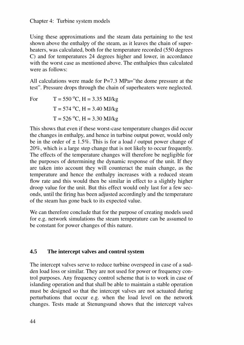
Chapter 4: Turbine system models
44
Using these approximations and the steam data pertaining to the testshown above the enthalpy of the steam, as it leaves the chain of super-heaters, was calculated, both for the temperature recorded (550 degreesC) and for temperatures 24 degrees higher and lower, in accordancewith the worst case as mentioned above. The enthalpies thus calculatedwere as follows:
All calculations were made for P=7.3 MPa=”the dome pressure at thetest”. Pressure drops through the chain of superheaters were neglected.
For T = 550 oC, H = 3.35 MJ/kg
T = 574 oC, H = 3.40 MJ/kg
T = 526 oC, H = 3.30 MJ/kg
This shows that even if these worst-case temperature changes did occurthe changes in enthalpy, and hence in turbine output power, would onlybe in the order of ± 1.5%. This is for a load / output power change of20%, which is a large step change that is not likely to occur frequently.The effects of the temperature changes will therefore be negligible forthe purposes of determining the dynamic response of the unit. If theyare taken into account they will counteract the main change, as thetemperature and hence the enthalpy increases with a reduced steamflow rate and this would then be similar in effect to a slightly higherdroop value for the unit. But this effect would only last for a few sec-onds, until the firing has been adjusted accordingly and the temperatureof the steam has gone back to its expected value.
We can therefore conclude that for the purpose of creating models usedfor e.g. network simulations the steam temperature can be assumed tobe constant for power changes of this nature.
4.5 The intercept valves and control system
The intercept valves serve to reduce turbine overspeed in case of a sud-den load loss or similar. They are not used for power or frequency con-trol purposes. Any frequency control scheme that is to work in case ofislanding operation and that shall be able to maintain a stable operationmust be designed so that the intercept valves are not actuated duringperturbations that occur e.g. when the load level on the networkchanges. Tests made at Stenungsund shows that the intercept valves

Turbine system models
45
were not actuated even during very large power output oscillations. Seediagram in Figure 4.8.
Another reason for omitting the intercept valves and their control sys-tem from the models used is that operation where the intercept valvestry to accomplish some kind of frequency control can never be toler-ated. The intercept valves are to serve as ”emergency brakes” for theturbine system only and neither their design nor their place in thesteam cycle allow for any continuous regulator service.
Figure 4.8 Unit 3. Intecept valve behaviour during a large output poweroscillation.
All tests made against the Stenungsund power station simulator showthat extremely unstable operation does occur IF the setpoints and theoscillations are such that the intercept valves are really trying to takepart in regulating the output power. This situation can occur if the staticdroop of the frequency control system is set to such a high value that asudden load reduction will correspond to a frequency increase suchthat the turbine speed moves into the activation area of the interceptvalves. In such a case we get a very unstable power regulation and theunit is not likely to be able to remain on line for very long. A typicalsuch case is shown in Figure 4.9, which is a run against the Stenung-
025
5075
100
125
150
MW
100
7550
250
%
5 10 15 s
Time
intercept valve position
generator power
0

Chapter 4: Turbine system models
46
sund power station simulator. It shows a case where 8% static droop isused and where has first been an initial load reduction, bring the fre-quency up to approximately 51 Hz. When a second load reduction,from 110 MW to 50 MW, comes, the frequency (and hence the turbinespeed) increases that much that the intercept valve starts closing andcontinues to close/open for each swing in frequency. As a result theoperation becomes extremely unstable, to an extent that such operationcould never be tolerated.
Intercept valve control is usually exercised by a control circuit that issensitive both to the absolute speed (rpm) of the turbine and to the rateof increase of the speed (positive derivative). The latter function isdesigned mainly to trap a condition where the turbine is acceleratingrapidly due to a load-loss condition and its settings are normally suchthat it will not be activated by normal network load changes and theircorresponding changes in frequency. The absolute speed sensing willhowever actuate the intercept valves as soon as the speed (=frequency)goes above a certain set limit, regardless of what caused the system toget to this condition and this effect must therefore be considered so thatthe system is not inadvertently driven into a speed region where theintercept system becomes active.
Figure 4.9 Simulator run. Intercept valve gets activated.

Turbine system models
47
The restraint that the intercept valves should be left out of the fre-quency control process sets a limit for how much governor static droopthat can be tolerated, when compared to the maximum uncompensated(meaning that there has been no operator power setpoint changes) loadchanges that are to be handled.
The maximum allowable static droop setting, compared to the maxi-mum sustainable uncompensated (meaning that there has been nooperator intervention by power setpoint changes) load reduction can becalculated thus:
By the definition of static droop:
(4.5)
where: K = static governor droop∆f = resulting frequency deviation from a load change = ∆PPn= nominal power rating of the unitf0= nominal network frequency
From this we get the maximum allowable droop as:
(4.6)
where: Kmax = maximum allowable static governor droopfi = activation frequency for the intercept valve controllerf0= nominal network frequencyPn= nominal power rating of the unit∆P= maximum load decrease that must be handled withoutoperator intervention
4.6 The condenser system
The condenser system can normally be represented as having constantpressure (=vacuum) and almost constant temperature. This is certainlytrue for all once-through water cooled condensers, as the variations intemperature of the sea or river water during a perturbation will cer-tainly be negligible. For air cooled systems corrections for changes incooling may be necessary, especially if the condensers are of the forced
K∆ffn------
Pn
∆P-------⋅=
Kmax
fI f0–
f0---------------
Pn
∆P-------⋅=

Chapter 4: Turbine system models
48
air or evaporative type with some kind of temperature control systemof its own. The same applies of course to an even greater extent forplants of the counter-pressure type. Here it will be necessary to modelthe behaviour of the counter-pressure and heat-exchanger part of theprocess in order to get a correct model.
4.7 A simplified steam cycle model
Under the assumptions made above (constant dome pressure, constantcondenser pressure and temperature and no intercept valve interaction)the model of the steam and turbine system can be simplified as shownin Figure 4.10.
Figure 4.10 Simplified steam cycle block diagram.
There is however one matter that complicates the modelling of thesteam cycle and that is the fact that steam is extracted at points inbetween for various purposes. Most of these steam extractions are rela-tively small and reasonably constant, as is the case for steam taken tothe pre-heaters or for running the vacuum ejectors that keeps up thecondenser vacuum. However there is in the case of the Stenungsundpower station one large steam extraction and that is for the pump tur-bine for the feedwater system.
The feedwater system in these units is run by a pump turbine thatextracts steam from the main cycle. In normal operation this steam is
Superheater &steam line delay
Condenser
Frequencycontrolsystem
Maincontrolvalve
LPturbine
HPturbine
MPturbine
Reheater
Constantpressure
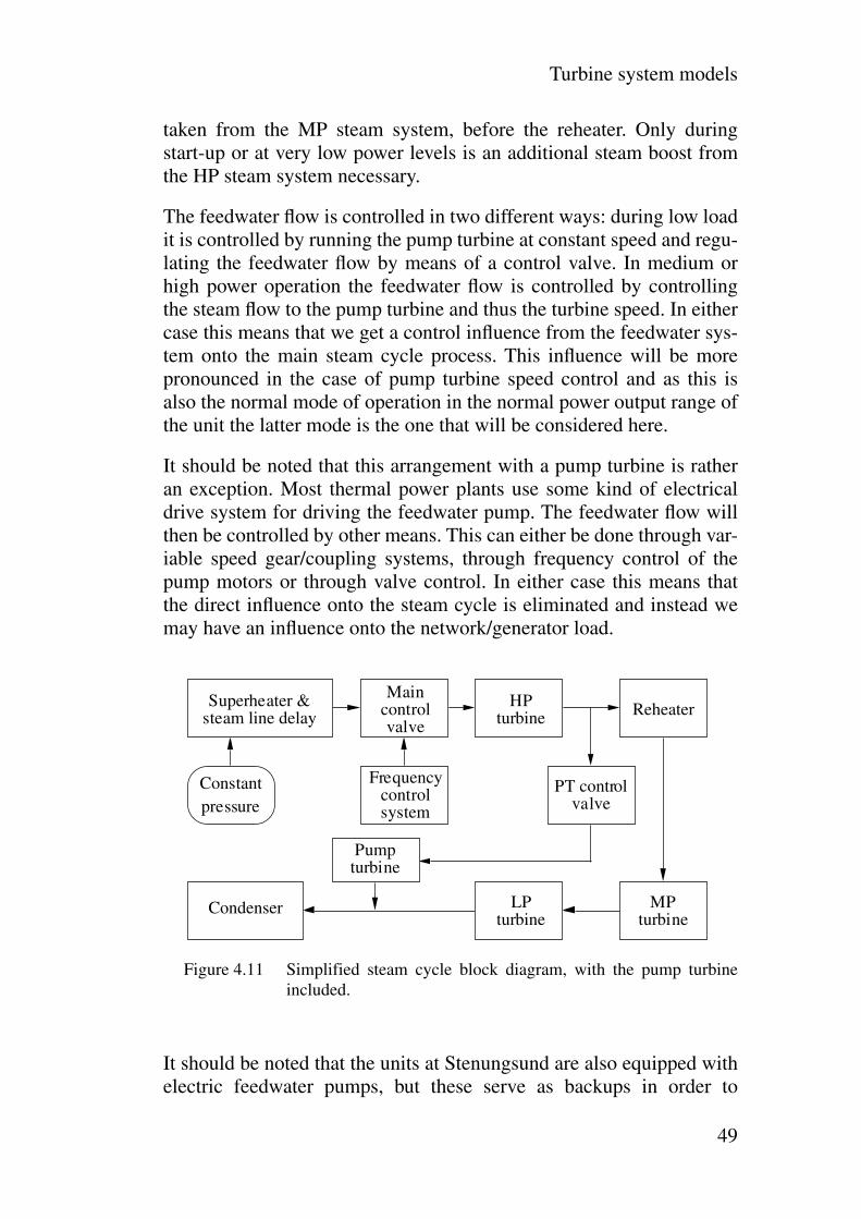
Turbine system models
49
taken from the MP steam system, before the reheater. Only duringstart-up or at very low power levels is an additional steam boost fromthe HP steam system necessary.
The feedwater flow is controlled in two different ways: during low loadit is controlled by running the pump turbine at constant speed and regu-lating the feedwater flow by means of a control valve. In medium orhigh power operation the feedwater flow is controlled by controllingthe steam flow to the pump turbine and thus the turbine speed. In eithercase this means that we get a control influence from the feedwater sys-tem onto the main steam cycle process. This influence will be morepronounced in the case of pump turbine speed control and as this isalso the normal mode of operation in the normal power output range ofthe unit the latter mode is the one that will be considered here.
It should be noted that this arrangement with a pump turbine is ratheran exception. Most thermal power plants use some kind of electricaldrive system for driving the feedwater pump. The feedwater flow willthen be controlled by other means. This can either be done through var-iable speed gear/coupling systems, through frequency control of thepump motors or through valve control. In either case this means thatthe direct influence onto the steam cycle is eliminated and instead wemay have an influence onto the network/generator load.
Figure 4.11 Simplified steam cycle block diagram, with the pump turbineincluded.
It should be noted that the units at Stenungsund are also equipped withelectric feedwater pumps, but these serve as backups in order to
Superheater &steam line delay
Condenser
Frequencycontrolsystem
Maincontrolvalve
LPturbine
HPturbine
MPturbine
Reheater
Constantpressure
PT controlvalve
Pumpturbine

Chapter 4: Turbine system models
50
increase the plant availability only. Their capacity is lower than that ofthe pumps driven by the pump turbines and hence a reduction in outputpower is required when operating with the electric feedwater pumps.For units 3 and 4 this means a reduction from 260 MW to 170 MW asthe maximum output power.
For a power plant of the type used at Stenungsund a simplified steamcycle block diagram will thus be as shown in Figure 4.11.
4.8 Power/steam consumed by the feedwater system
In order to allow for further simplifications we must try to estimate theamount of steam drawn to the pump turbine, as compared to the mainsteam flow. The data used refer to Stenungsund, units 3 and 4, but sim-ilar calculations can of course be made for other units or stations hav-ing the same kind of arrangement with a pump turbine, driven from themedium pressure steam.
The output power of the pump turbine is about 6.3 MW. In order tocompare with the generator output power we must reduce the gener-ated power by a certain coefficient in order to get the output power ofthe medium and low pressure stages of the main turbine only. Nor-mally these stages account for about 70% of the generated outputpower. With a nominal power of the unit being 260 MW, the power ofthe medium and low pressure stages will be about 182 MW. Thismeans that the steam extraction to the pump turbine will be in the orderof:
(4.7)
Thus the maximum steam extraction to the pump turbine is in the rangeof 3.5% when compared to power output of the two turbine stages thatare parallel to the pump turbine. If compared to the total unit output thesame figure gets about 2.4%. This is a fairly typical figure: most ther-mal power plants have a total power load from the auxiliary systems ofabout 4 to 6% of the plants output power, and the feedwater pump is byfar the largest auxiliary; typically accounting for about half of the aux-iliary power consumption.
αPp
Pn------ 6.3
182--------- 0.0346= = =

Turbine system models
51
For a fairly crude model this steam extraction can be neglected whenconsidering a control model for the turbine system. It is however possi-ble to go one step further and include this factor as well. The advantageis of course increased accuracy, but the cost in complicating the settingup of a model and of obtaining the necessary data from a particularplant do outweigh the advantages. The main reason for this is that thesteam extraction is linked to the feedwater control system, which con-trols the pump turbine. Therefore, in order to get a correct representa-tion of the behaviour of this system when dynamic response isconsidered one has to include the entire dynamics of the feedwatercontrol system, as well as the dynamics of the pump turbine and thefeedwater pump. Because of this the cruder model, where the steamextraction to the feedwater pump is neglected, will be used in the fur-ther analysis. However, before leaving this topic there will be a minoranalysis as to how an extra correction for the steam extraction to thepump turbine can be made.
For any centrifugal pump the power consumed when pumping liquidcan be written as:
(4.8)
where: P is the power consumed by the pumpη is the pump efficiencyp is the pressure difference inlet to outletQ is the flow rate of the liquid
If the efficiency can be assumed to be constant (on a real pump it is notreally constant but varies somewhat with the operating point of thepump, but as we are then considering a second order effect on a steamextraction that is only in the order of 3.5% to start with this effect canbe neglected here) then the power used can thus be said to be propor-tional to the flow rate Q.
In order for the boiler to maintain a correct water level (steam domelevel) the feedwater flow rate must always be made to balance with thesteam flow rate out from the boiler; i.e. the same number of kg/s ofwater must be pumped back into the boiler as the number of kg/s that isleaving it via the high pressure steam line. If this fails the dome levelchanges and quite soon a situation will occur that will trig first an alertand then if the situation gets worse a total trip of the unit. The reasonfor this is that operation with an incorrect dome water level is poten-tially hazardous for the plant: a low level may mean that some boilersurfaces run dry, thus leading to destruction through overheating, and a
P η p Q⋅ ⋅=

Chapter 4: Turbine system models
52
high level can lead to water being passed on the chain of superheatersand to the turbine, possibly causing turbine damage and also reductionof life expectancy for vital components due to rapid changes in temper-ature.
As already stated the dome pressure is assumed to be constant whenanalysing the units behaviour with regard to short term response. Thismeans that the output of the high pressure turbine is almost directlyproportional to the steam flow rate of the high pressure steam line. Thisassumes that the backpressure (pressure at the main discharge port ofthe turbine) for the high pressure turbine can be said to be reasonablyconstant, but this is normally the case.
The direct correspondance between steam flow rate and high pressureturbine output can be seen in all the measurements made and Figure4.12 shows a quite typical case, where unit 4 at the Stenungsund powerstation is subjected to three changes in load level, first down, then upand then again down.
Figure 4.12 Unit 4, HP steam flow and HP turbine power during step loadchanges.
Thus, if the feedwater system was absolutely ideal (zero response time,absolutely correct tracking at all times etc.) the power used by the feed-

Turbine system models
53
water system would be in direct proportion to the power of the highpressure turbine. This is however not the case with any real feedwatersystem. The number one deviation is that there is a significant timedelay in the system, due to the response time of the control system aswell as the delays caused by valve set times, steam travel and expan-sion time etc. This leads to that the feedwater flow will approximatelytrack the high pressure steam flow (and thus the high pressure turbineoutput power) with a certain, system dependant time delay. This can beshown clearly in Figure 4.13, which shows the performance of thefeedwater system during the test shown above (recorded at the sametest and showing the same time frame).
One can see that the feedwater system is tracking the changes in theHP steam flow with a time delay in the range of 8 to 10 s, with an ini-tial dead time of about 1 s before the system responds at all.
Figure 4.13 Unit 4, feedwater and steam flow during the test above.
However, more striking is the fact that whereas the feedwater system istracking the steam flow it does not do so to the full extent; instead itleaves a difference up or down. This can easily be understood when thecontrol circuit for the feedwater system is studied (Figure 4.14).

Chapter 4: Turbine system models
54
Figure 4.14 Stenungsund power station, units 3&4, feedwater control system.
Obviously the feedwater control depends not only on the steam flowrate but also on the current dome level, compared to the set point valueof the same. This is of course necessary as the tracking of the steamflow can never be a perfect match and even if it was additional com-pensation would be required as water can leave or enter the system byother means: a small quantity of water is constantly drawn from thebottom of the steam dome, and sometimes from other parts of the sys-tem as well, in order to reduce the amount of impurities in the boilerwater. On the other hand fresh water is added to compensate for anylosses.
The above means that a control model taking the effects of the steamused by the pump turbine is very difficult to construct and to get accu-rate. One can fairly easily model the steam flow dependent part, but thelevel dependant control depends on the history of the case, i.e. how theoperation has been PRIOR to the disturbance that we want to check theresponse to. There are really only three ways to deal with this:
1. to model the entire feedwater control system, complete with anintegrating part representing the flow differences integrated by thesystem volume.
2. to use a simplified model where the dome level is assumed to becorrect (i.e. equal to its set point value) prior to the situation that onewants to test. In such a case a simple representation of the feedwatersystem will do, typically involving only the steam flow rate as thecontrolling variable.
+
–+
++
–
Dome level set point
Dome level
HP steam level
Feedwater flow
Signal to pump
turbine controller

Turbine system models
55
Figure 4.15 Simple turbine system model with steam-driven feedwater pumpaccounted for. C1 is a proportionality constant linking the HPsteam flow to the HP turbine power. This constant will depend onthe current dome pressure. C2 is a proportionality constant linkingthe required feedwater pump power to the feedwater flow. Alsothis constant has a depends directly on the dome pressure, as thepump power required is roughly proportional to the pumppressure, which must balance the dome pressure. T1 is the timedelay of the feedwater system and its control system.
3. To use a much simpler model, neglect the time delay involved andsimply reduce the output power of the medium and low pressureturbines by a set figure calculated based on the power data of thefeedwater pump an the MP and LP turbines; in this case 3.5%. Thiswill normally give sufficient accuracy and gets around many of themodelling problems that come up if the feedwater system has to beincluded in the main turbine model. This approach is therefore usedin the following.
Figure 4.16 Simple model where an electric feedwater pump is used.
The above discussions have been based on a feedwater pump driven bya pump turbine, but a very similar reasoning will apply to the more
HP turbine power HP steam flow
MP + LP turbine power
feedwater
C1 C2 T1
-+
++
total unit output
pump power
HP turbine HP steam
MP + LP turbine power
feedwaterpump power
C1 C2 T1
-
+++
Totaleffectiveunitoutput
power flow

Chapter 4: Turbine system models
56
common case where the feedwater pump is driven by an electric motor.In this case there is no steam extraction for this purpose, but the motorpresents a load on the network and thus on the generator and the resultbecomes the same, except that the pump power should, for the case thatis described under 2. above, instead be subtracted from the total power:
Note that the output here is the effective output, taken as the generatoroutput minus the power consumed by the feedwater pump motor.
4.9 High pressure turbine response
The high pressure turbine responds extremely fast to any changes ofthe control valve position. As the control valve is normally locatedright next to the turbine inlet port there are no time delays pertaining tosteam line lengths or system volumes involved and the response ishence almost instantaneous.
A typical recording (Figure 4.17) shows how the high pressure turbineassembly responds to a step change in the control valve position withinless then half a second. The response at the ”bottom” is slowed downsomewhat by the fact that there are also two axial low pressure turbinesin the HP assembly; if the output of the HP radial stage could be meas-ured separately the response would be even more distinct.
If the downramp part is enlarged one can see that the response is actu-ally extremely fast, as can be seen on the diagram in Figure 4.18.
From this diagram can be seen that the high pressure turbine assemblypower tracks the position of the control valve within a fraction of a sec-ond, the time shift being less then 0.1 s.
Another interesting effect can also be clearly seen: there is a kind ofback-lash effect in that the power oscillates up for a very brief moment,following the initial drop. This can not be explained by the behaviourof the valve, as the valve position recording, which is measureddirectly from the valve position potentiometer, shows no such oscilla-tory motion or bounce effect. The explanation must instead come fromthe steam dynamics of the high pressure steam line and be due to apressure variation in the steam line. This is further discussed in the nextparagraph which addresses the dynamic effects of the steam lines.

Turbine system models
57
Figure 4.17 Unit 4; HP turbine response related to the control valve position.
Figure 4.18 Enlargement of the downramp in Figure 4.17 with the HP steamflow plotted.

Chapter 4: Turbine system models
58
4.10 Effects of the steam lines
The main steam lines are of considerable length and cross-section anddo thus hold a considerable amount of steam. This steam is in motionand forms a dynamic system. Primarily three effects of the steam linescan be expected:
1. A pressure drop, which according to the laws of kinematics isproportional to the square of the steam velocity.
2. A time delay which relates to the length of each line compared to itssteam velocity.
3. An induction effect in that it tries to resist all changes in steamvelocity / steam flow: if the flow is increased rapidly it takes timeand power to accelerate the steam and if it is reduced suddenly themomentum of the steam tries to keep the motion up.
As for the pressure drop this is of prime interest if one is investigatingthe overall efficiency of a plant at the design stage, but it is also ofinterest with regard to the dynamic response of the plant. Though all itmeans in steady-state operation is a slightly (very slightly if the systemis properly dimensioned) reduced output power, especially at full loadwhere the steam flow is at maximum, it can give rise to certaindynamic effects that will be discussed in the following, as it can lead tochanges in the admission pressure present at the inlet port of the con-trol valve.
The time delay is of little interest with regard to the dynamic responseif we are considering the high pressure steam line. The reason for thisis that the main control valve is not located at the beginning of the linebut at the very end, in immediate proximity of the turbine admissionport. This is done exactly in order to minimize the time delay causedby the HP steam line. The distance between the main control valve andthe admission port can of course not be made equal to zero for designreasons, but it is kept very low, as the valve is usually located rightalong the side of the turbine.
The above applies to the high pressure steam line only. When it comesto the medium pressure steam lines the length becomes significant ashere there is no control valve at the end. There are the intercept valves,but as mentioned earlier these should normally always be open whenwe have some kind of operation that is at least reasonably stable.Instead the steam inlet control to this system is simply exercised by the

Turbine system models
59
high pressure system: what ever steam that comes out of the high pres-sure turbine outlet port will, with associated time delays, travel throughthe medium pressure steam lines back to the boiler, through thereheater and then through the steam lines again back to the turbine sys-tem, to enter into the medium pressure turbine. This long path of travel,plus that the steam will not even be available to the medium pressuresystem until it has expanded its way through the high pressure turbine,means that the response of the medium pressure system to any changesin the control valve settings will be considerably delayed. A similardelay will apply as the steam moves on to the low pressure turbines,but this delay is much shorter as there is no reheater involved and thesteam lines are much shorter as they do not go back to the boiler butinstead they just transfer the steam from one part of the turbine systemto another.
As mentioned in Chapter 3 it has not been possible to separate themeasured power from the medium and the low pressure systems.Instead the two systems have been considered as one thermodynamicsystem and the time delay that has been established as a part of themodel refers to this combined system as related to the high pressuresystem.
For the case of the Stenungsund power station, unit 4,the time delayhas been measured for various types of sudden load changes and typi-cal cases are shown below, Figure 4.19 showing a step increase of thenetwork load and Figure 4.20 a step reduction.
Describing the system as a first order system and defining a time con-stant as per the normally used definition that the change in the outputvariable should be complete to 63% one can determine this time con-stant for the steam system delay from the high pressure system to thecombined medium and low pressure system. This figure will have aslight uncertainty in it, in that the input in the form of the change of theposition of the control valve is not a real step change. Due to the factthat the control valve can only move with a finite speed, plus that thefrequency control system has some damping/delay built into it, thisinput will always be a gradual change rather then a step function. Dueto the fact that the control valve is normally built so that it closes muchfaster than what it opens the two cases, increasing or decreasing power,will have to be treated differently.

Chapter 4: Turbine system models
60
Figure 4.19 Unit 4; turbine responses during a power increase.
Figure 4.20 Unit 4; turbine responses during a power reduction.

Turbine system models
61
Taking the case in Figure 4.20 the time constant for the closing of thecontrol valve, defined as above as the 63% limit, is about 0.7 s. This isin the range of 7 times the corresponding time constant of the MP/LPturbine system, and it is a reasonable estimation to regard the input sig-nal as a step function, in which case the turbine time constant can bemeasured to approximately 5.2 s. However observing the curve one cansee that this time consists of two parts: a dead-time of approximately0.7 s and a time constant for the consequent change of approximately4.5 s.
For the case of the power increase as shown in Figure 4.19 it is harderto get a correct estimation of the MP/LP turbine time constant. Thecontrol valve moves slower and the approximation used above is nowless correct. The slower motion of the control valve will naturally slowdown the final response. On the other hand the control valve motionshows a larger overshoot in this case and that tends to act the oppositeway. The larger overshoot is a natural consequence of the fact that thevalve moves slower on opening then on closing, as the control valveposition is used as the feedback loop controlling the valve position. Ifone does not compensate for any of the above the time constant asmeasured for the power reduction case will be 4.2 s, which can asabove be divided into a dead-time of 0.7 s plus a first time system timeconstant of approximately 3.5 s. The turbine seems to respond some-what faster on increase then on decrease. The most plausible explana-tion is that in the case of the power reduction there is a slight additionexpansion time for the steam trapped inside the turbine whereas for theincrease the steam will hit the vanes with less delay. However, an anal-ysis of several test cases show variations in the order of one second,primarily due to difficulties in getting a correct assessment of the timeconstant when the input signal is not a perfect step function. Thereforea cruder estimation, using the same time constant for increase anddecrease will be used in the following.The fact that the dead-time issimilar in the two cases is natural, as this consists of mere travel timefor the steam pressure wave through the high pressure system and thereheater plus the associated steam lines. The MP and LP systems willnot be affected by a change in the control valve position until this pres-sure wave reaches the inlet port of the MP turbine. Note that the factthat this wave has reached the system is only the beginning of thechange process, for the actual bulk of the steam to do the same takeslonger and as a result the first order time constant is considerablylonger.

Chapter 4: Turbine system models
62
An extra factor to be considered is of course the actions of the controlvalve limiter. This one will be discussed in the following and is ofcourse of prime importance when it comes to determining how the unitcan respond to a very fast increase of the load.
As for the dynamic effects of the steam in motion this can be clearlyseen only in cases where there is a very sudden and fairly substantialchange in the steam flow rate. The two cases of a sudden reduction andof power increase must be treated separately as there are two somewhatdifferent phenomena that occur. The first case to be considered is thepower reduction, where the dynamic effects are most obvious.
Figures 4.21 and 4.22 show the behaviour of unit 4 at the Stenungsundpower station when subjected to a step-wise load reduction in the sim-ulated network (simulated island operation, real unit under test). Theload reduction is the same in both cases. The difference is that in Fig-ure 4.21 the total moment of inertia of the system has been set equal tothe total for all four units at Stenungsund, assuming that they are allon-line, but that only unit 4 is responsible for the frequency control; theother units being operated with an active governor dead-band, whereasin Figure 4.22 the moment of intertia has been set to that of unit 4alone; thus assuming that this one is the only unit on the island net-work. In the case of all four units the changes become slower and nodynamic effects of the kind described above can be noticed, neither onthe power reduction nor on the. In the case of the single machine how-ever, the changes are rapid enough to produce a significant dynamiceffect, clearly noticeable as on oscillation of the high pressure turbineassembly output power right after the drastic reduction. Note that thereis no corresponding oscillation of the control valve position. Thisshows clearly that we are dealing with a steam dynamics phenomenaand not with some kind of unstable controller action. Network loadversus generator oscillations are automatically ruled out as during thetest the unit was, as is normal for this test method, synchronized ontothe normal, strong network. Also, the latter is ruled out by the fact thatthe oscillations are clearly visible on the steam flow curve, whichwould not be the case if they were network induced.
The same dynamic effect is seen more clearly in Figure 4.23, where thesame unit was subjected to a faster and more drastic power reductionby the sudden injection of a larger control signal. Here one can seevery clearly that following the initial power drop there is a markedincrease in power and in the steam flow and this without that the con-trol valve bounces back in any way.

Turbine system models
63
Figure 4.21 Unit 4; system responses to a load reduction. High J value.
Figure 4.22 Unit 4; system responses to a load reduction. Low J value.

Chapter 4: Turbine system models
64
Figure 4.23 Step power reduction response.
The extra “boost” of the power and steam flow is caused by a pressurebuildup across the control valve. When the steam is in rapid motionand the valve quickly closes, the momentum of the steam tries to keepup the steam velocity and as a result the steam is compressed on the upside of the valve. At the same time the same effect causes a drop in thepressure on the down side of the valve. The result is an increased dif-ferential pressure across the valve and hence and increased steam flow.The same effect will arise whenever a rapid flow of a liquid or a gas issuddenly interrupted by an obstacle, in this case a closed control valve.A simple figure (4.24) below with a fluid moving in a pipe illustratesthe effect.
Figure 4.24 Dynamic effects when the flow of a fluid is suddenly restricted.
fluid velocity
pressure buildup reduced pressure
suddenly inserted obstacle

Turbine system models
65
The dynamic pressure effect acts as a pressure wave that travels backand forth in the system. E.g. it will bounce in between any two pointswhere the characteristics of the steam flow path changes in a majorway. It seems plausible that the main such bouncing effect will be inthe high pressure steam line; i.e. between the control valve and the lastsuperheater, superheater three in this case. The recording above clearlyshows this oscillatory behaviour.
This dynamic effect is undesirable in several ways. One is that anyoscillatory changes of the turbine power means an increased mechani-cal load onto the turbine shafts. In power stations with long turbineshafts, which is common for stations having a one-all turbine shaft,there is always a risk that if such oscillations are close in frequency tothe natural mechanical resonance frequency of the shaft/turbine systemthese oscillations can grow much larger than anticipated and in extremecases there can be a risk of fractioning the shaft assembly.
Another drawback resulting from this dynamic effect is that we get apower boost at a time when we do not want it; that is when we havehad an overfrequency and thus a sudden reduction in power. Havingthis extra power boost will just drive the frequency still a little higher.
The third problem with this dynamic behaviour is that we may getproblems with the auxiliary systems, in particular with the feedwatersystem. In virtually all thermal power stations the steam flow is used asa variable controlling the feedwater system. Often a derivative action isincluded in this controller so that any increase in steam flow automati-cally will lead to an increase in feedwater. In a case like that of Figure4.23 this is an incorrect action. We have just had a drastic reduction inpower and we do not want an increase in the feedwater flow at thispoint. Oscillations in the steam flow can therefore lead to oscillationsin the dome level, as a result of that the feedwater controller can nothandle the oscillating situation properly. If the dome level oscillates toomuch this can lead to a total trip of the unit. This problem is discussedfurther in Chapter 7.
What has been said above about the feedwater system also applies tothe firing fan control system. Here we often have a dependency onchanges of the steam flow so that we can get incorrect action in caseslike this. Also this is discussed further in Chapter 7.
The dynamic oscillations of this kind should normally not be includedin a turbine model as such, as they do not occur in normal operation
Chapter 4: Turbine system models
66
where steam flow changes are less rapid. Instead it should be thoughtof in the design of the control system for the control valve that oneshould try to eliminate or at least minimize these oscillations. Withmodern, computerized control systems this should be fully possible,e.g. by including software that will detect a rate of change above a cer-tain value that is considered critical with regard to such oscillations andthen take appropriate action, e.g. by moving the control valve in anoptimized fashion. The oscillations in this case have a period time ofabout 0.8 s in this case (this time is of course different for every instal-lation and will depend on pipe lengths and cross-sections etc.).Thecontrol valve moves in a fraction of a second (closing time 0.2 s asspecified for full range for this unit) and is thus fast enough so that itcan be controlled in an intelligent manner in order to minimize theseoscillations.
When the power is instead rapidly increased, corresponding to a rapidopening of the control valve, we get two dynamic effects. One is theabove effect in reverse, in that due to the change of momentuminvolved in increasing the steam velocity it takes finite time, as no mat-ter can be accelerated instantaneously. This merely leads to a slowingdown of the process, plus that we also here get a pressure wave thattravels in the system and can cause various difficulties. In this casethese are however of little actual concern, as the control valve opensslower than it closes and thus it is rare that we get a flow increase thatis rapid enough to cause any sizeable oscillations.There is however oneadditional dynamic effect that is involved in this situation. This is dueto a change in steam pressure at the inlet point of the turbine system.We have earlier concluded that the dome pressure can be regarded asconstant for short term changes, but this applies to the dome pressureand not to the pressure present at the inlet port of the control valve. Inbetween we have the chain of superheaters plus the high pressuresteam line and we have some losses (=pressure drops) as the steampasses through these. These pressure losses are by the laws of gas kine-matics proportional to the square of the steam velocity:
(4.9)
where: ∆p is the pressure drop
v is the steam velocity
C is a proportional constant.
∆p C v2⋅=

Turbine system models
67
The steam velocity is given by:
(4.10)
where: Q is the steam flow rate
A is the cross-section of the pipe etc. at a given point
v is the steam velocity at that same point
As the cross-section does not change in time we get:
(4.11)
where: C2 is a new constant
As the steam flow increases with an increase of power we get onincreased pressure drop through the systems and hence a lower pres-sure present at the control valve input port, the latter being:
(4.12)
where: pinput is the pressure at the input port of the control valve
pdome is the dome pressure
The result is that when we get an increase of the steam flow (i.e. thecontrol valve opens) we get a reduction in the input pressure. Thisreduction is small, as minimal losses must always be a design objectiveand hence the cross-section so chosen that this drop is kept low, but notcompletely insignificant. But when the valve has just opened this effectis not applied instantaneously, as the high pressure steam line acts as areservoir and the pressure will therefore be kept high for a very shortwhile, until the effect of the pressure drop is noticeable. This leads toan extra power boost for a very brief moment following the opening ofthe valve. This effect can be noticed in the recording in Figure 4.25,from unit 4 at the Stenungsund power station. Note there is no over-shoot in the motion of the control valve, but that we get what looks likean overshoot effect on the steam flow and hence on the power output.
This dynamic effect is not insignificant. In the case above it representsan extra power boost with a top amplitude of about 3 MW. As theapplied load increase was 15 MW it represents 20% of the increase and
v QA----=
∆p CQA----
2⋅ C2 Q
2⋅= =
pinput pdome ∆p– pdome C2 Q2⋅( )–= =

Chapter 4: Turbine system models
68
it has a pulse duration of about 1 s. If a detailed model is to be made ofthe unit, e.g. to study possibly oscillatory behaviour in island opera-tion, in a critical case, it may be necessary to model the same. This canbe done, as the steam flow rate, the flow resistance of the superheaterand of the steam lines, as well as the volume (=storage capacity) of thesteam lines, are all known quantities. In order to get a simple modelthat can be used for more normal studies of networks in emergencyoperation and similar this effect can however be neglected, due to itsshort duration.
Figure 4.25 Unit 4; system response as the control valve opening increases.
As mentioned earlier all oscillations are negative from the point of thestresses presented unto the mechanical systems. This effect is howevera one-swing phenomena and should not be able to cause any majorproblems. From the network point of view this effect is instead a posi-tive one, as it produces an extra power boost at a time when power isneeded; i.e. when there has just been a load increase and a correspond-ing drop in frequency.

Turbine system models
69
4.11 The control valve and the control valve limiter
The control valve itself has a valve characteristic that is not quite linearif one considers its entire operating range, but in the mid-range, whereit is normally used for any operation that involves frequency controland that is at least reasonably stable it can be assumed to be linear.Also, a compensation for the main non-linearities of the valve is nor-mally included in the control system. However its actuator is normallyasymmetric, in that it is designed to close the valve faster then it canopen. Several different designs are possible here; either consisting ofone main valve that can be operated at different speeds or one governorcontrol valve plus a fast-acting extra shutdown valve, or as an in-between a valve where there are two actuators, one fast and one slow,connected to the same valve.
The normal mode of operation is the slow mode. This is by no meansslow e.g. compared to say the vane controllers of hydroelectric powerstations, which are way much slower. However, even though this modeis relatively fast by comparison, it is normally not fast enough for theextreme situations, such as a sudden load-loss at full power. In such asituation the valves must be closed extremely fast to prevent the turbinefrom reaching overspeed. A typical design is shown in Figure 4.26.
Figure 4.26 Steam control valve.
If fast operation is obtained by a separate valve or by a separate extraactuator on the main valve, then this usually employs heavy springs to
fast closing valve fast closing valve
normal control valveset of slide valves
actuator shaft
inlet inlet
outlets

Chapter 4: Turbine system models
70
close the valve and a corresponding opening of the same is thereforeextremely slow compared to its closing time. This fast closing shouldonly be actuated in cases where there is an immediate problem withoverspeed (such as a load-loss condition). This mode does not have tobe modelled as part of the turbine model, as it should not be activatedin normal operation, even on a very unstable and oscillating network. Ifit is activated then there is normally no way back, as opening it again istoo slow, so in such a case the unit will have to be tripped from the net-work, re-started and re-synchronized.
The control valve limiter has to be given special attention in caseswhere there are large perturbations on the network. Most power sta-tions have some kind of limiter, however the designs vary. The purposeof the limiter is primarily to prevent excessive step increases of thevalve position and hence of the steam flow, as this could lead to dam-ages. On older systems (such as units 1 & 2 at the Stenungsund) thislimiter is completely manual and is set by the station operators to asuitable value a bit above the current point of operation, whereas moremodern systems (e.g. units 3 & 4 at Stenungsund) have some kind ofautomatic tracking, so that the limiter runs itself, moving with thechanges of the power and allowing for slow changes while still block-ing rapid and large increases.
Several tests run against the power station simulator at Stenungsundshow clearly that the ability of the power station to exercise frequencycontrol, without excessive oscillations of both power and of frequency,deteriorates considerably if the station comes into an oscillating modeto the extent that the limiter gets activated. This is natural, as suddenlywe have slowed down one side of the regulating process, in thatincreases can only take place slowly, whereas decreases can still befast. It must therefore be one objective in obtaining a well functioningisland operation mode that one can operate the station in such a way sothat the control valve limiter is not at all taking part in the process.Note that for normal load increases, which for a network of limited sizehave been estimated at a maximum of 5% of the load the system is notat all active, as the normal tracking margin is in the range of 10%.
The recordings below, from Stenungsund unit 4, shows the behaviourof the limiter and the control valve when the unit was subjected to aseries of step load changes. In Figure 4.27 a network with all four unitsat Stenungsund on line was considered, and as a result the totalmoment of inertia was high enough to slow down the changes enough

Turbine system models
71
to keep up with the rate of change of the tracking limiter and as a resultthe limiter never became active.
Figure 4.27 Unit 4; control valve limiter behaviour during a load increase witha high J value.
Figure 4.28 on the other hand shows a test case where the correspond-ing simulated island network has no generator other then that of unit 4on line. The moment of inertia is now smaller and as a result allchanges get more rapid. Still, it takes a fairly large power change to forits control valve to get into contact with the limiter. In two cases thishas occurred and as expected the shape of the curve is altered in thesecases and it can be concluded that this the limiter had a significantinfluence on the process. In these cases the load increase was equal toabout 8 and 15% of the output power (thus somewhat beyond expectednormal load fluctuations) and the limiter became active but only for ashort time. It did in this case not result in any problem in maintainingthe network frequency, but for a complete model for the case thateffects of large disturbances are to be studied, then the limiter must bepart of the model. These models will of course be very different for dif-ferent power stations, due to the wide scope of designs in this field, sothe models stated below apply to the Stenungsund station only. They

Chapter 4: Turbine system models
72
can of course also be applied to other stations with the same type ofcontrol systems.
Figure 4.28 Unit 4; control valve limiter behaviour during load changes. LowJ value.
Figure 4.29 shows the second step increase from Figure 4.28, wherethe limiter had the greatest impact. Studying the response from the twoturbine assemblies one can see the action of the limiter.
As can be clearly seen the limiter prevents the control valve from open-ing as fast as it would do if no limit was imposed. As a result the powerincrease from the turbines is also slowed down. The high pressure sys-tem, which normally would respond within a fraction of a second, nowreaches its maximum power after about 6 s, and the medium pressuresystem after about 17 s, counting from the time of the load change,which is equal to the time when the frequency of the simulated networkstarts changing. As a result it takes quite long before the system finallyrestores the network frequency to the new operating point (=previousfrequency minus the difference caused by the static droop).

Turbine system models
73
Figure 4.29 Unit 4; detail of the second step increase in Figure 4.28.
A control valve limiter of the type used for units 3 and 4 at Stenung-sund uses one sole input parameter: the control valve position and italso acts on (limits) exactly the actuator signal controlling that samevalve position. There is also a manual mode, where the limiter is con-trolled by the operators by giving increase/decrease signals, but theautomatic tracking mode is the normal mode of operation. The timeconstant for this particular installation is 50 s and the normal trackingmargin is 10%, giving a control model as in Figure 4.30.
Figure 4.30 Tracking control valve limiter.
valve opening requestfrom the control system
1Tv s
valve actuatorposition
150 s
manual control
+
+0.10
0
valve pos.limit

Chapter 4: Turbine system models
74
4.12 The frequency control system
The frequency control system itself is of course of prime importancewhen it comes to the units ability to maintain proper operating fre-quency. There are very many design concepts for these systems and thesystem used at Stenungsund, units 3 and 4, which will be the base forthe discussion below does only represent one such design. The samedesign concept in the sense of the control blocks involved is howeverfound in virtually any governor system.
Basically there are five generations of frequency control equipment inuse in different power stations throughout the world:
1st generation, used up to the 1930s, had completely mechanical gov-ernors, with centrifugal controllers as the frequency sensing elementand purely mechanical or hydraulic control elements. These systemsoffered no more than a basic setting of a couple of main variables, suchas the frequency set point and the governor droop. It should be notedthat very many of these systems are still in active duty and they areoften remarkably reliable, mainly due to their simple design and thehigh degree of mechanical perfection that was used in manufacturingthem.
2nd generation used electrical controllers, but with no electronic partsin it, amplification by rotating amplifiers or transductors, only in rarecases with vacuum tubes and similar. These systems are now in mostcases replaced by more modern ones, as lack of both spare parts andstaff with the required technical knowledge of these systems make ithard to maintain them. Their overall reliability is usually actually lowerthen for the older 1st generation systems.
3rd generation used electronic control systems, with transistors andother solid-state devices, sometimes with transductor amplifiers orsimilar for the more high-powered parts of the systems. Also these sys-tems are now getting obsolete and are being replaced by more modernones. This is often easily feasible as the systems are designed for lowlevel electrical control and it is often possible to keep the costly partsand just replace the electronics with modern systems.
4th generation used linear integrated circuits, primarily operationamplifiers and allowed for a more exact and sophisticated control ofthe behaviour of the systems. Many such systems are in operation andas this technology has as of yet no maintenance or spare components
Turbine system models
75
problems there are so far no compelling reasons for replacing/modern-izing it, unless it is done as a part of a general upgrade of the whole sta-tion or the entire control equipment.
5th generation is the state of the art today, with digital, computerizedcontrol systems. These allow for tailoring the control characteristics invirtually any way that the designer wants and allow for easy ways ofadding several different control modes, so that e.g. the system can,automatically or by operator command, switch to a different set of con-trol variables if certain unstability criteria with regard to the network,such as frequency variations beyond set limits, are met. A drawbackwith this generation is that the extremely fast development in the fieldof microcomputers make the systems obsolete quite fast and it is there-fore highly unlikely that these systems will attain anywhere near thelifespan of the older control systems.
The test / simulator system designed within this research project can beapplied to all cathegories of control systems, except the 1st generation.As the latter has no electrical input for the frequency there is no waythat the system can be fed a simulated control signal and hence thebasic idea of this technique can not be applied.
A block diagram for the frequency control systems of units 3 and 4 atthe Stenungsund power station is shown in Figure 4.31. This controlequipment can be said to belong to the third generation as describedabove. Units 1 and 2 at Stenungsund have more modern control sys-tems, belonging to generation four as above.
Two of the systems shown in Figure 4.31 can for modelling purposesnormally be eliminated. This applies to the dome pressure turbine con-trol and the system for controlled shutdown. As for the linearizer thiscan sometimes be eliminated, but if an accurate model is to be obtainedit must be included.
The purpose of the linearizer is to compensate for the fact that if thecontrol valve is opened only to a small percentage of its full openingthe effect of a certain change of its position is greater then if we makethe same change in a situation where the valve is already open to alarger extent. This is a consequence of the laws of kinematics and italso involves a certain compensation for non-linearities of the controlvalve itself. Sometimes this block is therefore referred to as a controlvalve non-linearity compensation.

Chapter 4: Turbine system models
76
Figure 4.31 Frequency control system, Units 3 & 4, Stenungsund powerstation.
In the case of units 3 and 4 at Stenungsund the linearizer is modelled tohave the characteristics shown in Figure 4.32.
Figure 4.32 Model curve for the non-linearity compensation of units 3 & 4 atStenungsund.
The linearizer can be removed from the model by simply assuming thatthe valve together with the behaviour of the steam form a system that islinear. After all, what we are interested in is the actual amount of steam
main control valve
control valveactuator
frequency set point
frequency(from turbinetachometer)
–
+
speed / powerset point
limitersystem
(see sec.4.10)
linearizer
Min.select
–+
–+
1droop
dome pressureturbine control
system forcontrolledshutdown
C2
1+ C1. T1 . s1+T1
.s
0.0HP steam line
controlvalveposition
1T2
. s
45 % 100 %
0.77
0.90
valve position
feedback signal multiplier
00
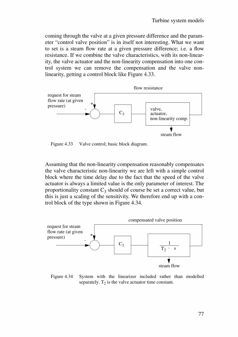
Turbine system models
77
coming through the valve at a given pressure difference and the param-eter “control valve position” is in itself not interesting. What we wantto set is a steam flow rate at a given pressure difference; i.e. a flowresistance. If we combine the valve characteristics, with its non-linear-ity, the valve actuator and the non-linearity compensation into one con-trol system we can remove the compensation and the valve non-linearity, getting a control block like Figure 4.33.
Figure 4.33 Valve control; basic block diagram.
Assuming that the non-linearity compensation reasonably compensatesthe valve characteristic non-linearity we are left with a simple controlblock where the time delay due to the fact that the speed of the valveactuator is always a limited value is the only parameter of interest. Theproportionality constant C3 should of course be set a correct value, butthis is just a scaling of the sensitivity. We therefore end up with a con-trol block of the type shown in Figure 4.34.
Figure 4.34 System with the linearizer included rather than modelledseparately. T2 is the valve actuator time constant.
C3valve,actuator,non-linearity comp.
flow resistance
steam flow
+-
request for steamflow rate (at givenpressure)
C3
compensated valve position
steam flow
+-
request for steamflow rate (at givenpressure)
1T2
. s

Chapter 4: Turbine system models
78
Note though that in the case of the Stenungsund units 3 & 4 this simpli-fication will lead to another complication. This is because the settingvalue used for the tracking control valve limiter uses the “raw” controlvalve position as its input. If we will use the simplification describedabove we must therefore apply a compensation to the limiter controlcircuit, as otherwise we get an incorrect value for the margin betweenthe current valve position and the limiter, as this margin is for steady-state operation set to 10% of the actual control valve position. Sowhereas the linearizer can be neglected for crude models it must still bekept in the circuit if a detailed and highly accurate model of units withthis design should be made.
The dome pressure turbine control system is designed to prevent exces-sive pressure drop in a situation where the frequency control systemdemands more power, and hence more steam, than what the boiler cansupply at that given moment. In a situation like this the dome pressureturbine control system will become active and will reduce the outputpower in order to preserve steam so that the steam pressure of the domecan be held to an acceptable level. When this system is activated ittakes over control from the frequency control system and the unit dropsout as far as performing frequency control goes. Clearly, if thismachine is the only one on line this means that we can no longer main-tain the network frequency and hence the frequency will drop. Thereare then only two ways that the network can be returned to a controlla-ble situation: either the boiler manages to respond so that it delivers thesteam required, hence rising the dome pressure and de-activating thedome pressure turbine control system, or the load is reduced throughload shedding to such a level that the steam available allows the unit tofind a new stable point of operation.
From this can be concluded that for modelling the power station as apart of setting up a functioning island operation network this systemcan be eliminated. The operation must always be such that a reasonablemargin is maintained with regard to the minimum required dome pres-sure and hence the boiler system must be taken into account in order todetermine as to whether this puts restraints on the possible conditionsof operation. For a further discussion of this see Chapter 5, where theboiler system and its behaviour is discussed. For now, we conclude thatthis system need not be included in the turbine / steam system model,as it should never become active.
The systems for controlled shutdown should also remain inactive dur-ing any acceptable operating conditions. These systems are activated

Turbine system models
79
by some of the various protection systems of the power station andreduce the power in order to obtain safe operating conditions when thesecurity situation so require. In the case of the Stenungsund station,units 3 and 4, there are two levels of controlled shutdown or powerreduction. One is reduction to a minimum steam flow as required forthe cooling of the turbine, the other is reduction to 50% of the ratedpower. As an example a controlled shutdown can be ordered if the fuelto power differential protection is activated; i.e. if the amount of fuelinjected does not stand in a reasonable relation to the output power ofthe unit at the time. This protection is to protect against bad fuel oil,primarily against large amounts of water in the oil. In such a case thereis no immediate danger and hence no need for tripping the unit, butinstead a controlled shutdown will be ordered. Several other protectionsystems give the same kind of response.
As these systems are part of the unit protection they should obviouslynot in any way interfere with normal operation of the unit. If they areactivated they take over the control of the output power from the fre-quency control system and should this unit be the only one on line atthe time it will, short of possible operator intervention, lead to the trip-ping of the unit and a blackout on the network. Again we have a situa-tion where a condition that can not be tolerated in operation does notneed to be modelled, as if we get to this condition it is normally too lateto save the system anyhow. There is an exception to this and that is thatunder certain circumstances the fuel to power differential can be trig-gered if we have extreme power reductions; i.e. drastic disconnectionof load on the network. Test against the power station simulator at Ste-nungsund showed that e.g. a sudden load reduction from 250 MW to100 MW could trigger this circuit. In such a case operation can berestored by the operators, who can override or reset the controlled shut-down. It is however still not meaningful to model these systems as theonly way out of an ordered shutdown, other then a unit trip, is by oper-ator intervention and the behaviour of the operators, their alertness etc.can not be modelled in any case.
4.13 The importance of the feedback variable
A design factor that must be considered is what feedback variable thatis used in the second level control loop that controls the unit outputpower to a desired level. In the case of the units 3 & 4 at Stenungsund

Chapter 4: Turbine system models
80
this quantity is, as shown above, the control valve position. This has thedrawback that one has to introduce a linearizer to get a more linearbehaviour, but otherwise the use of the valve position for feedback isan excellent choice, as the valve position is not at all under any directinfluence of any possible events in the power network. We get a secondlevel control system of the type shown in Figure 4.35.
Figure 4.35 Control valve position used as the feedback variable.
If we instead use the electrical output power as our feedback variablewe get a control circuit of the type shown in Figure 4.36.
Figure 4.36 Generator output power used as the feedback variable.
It would be tempting to think of the system shown in Figure 4.36 as thepreferred system, as we get the true electrical power output from thegenerator as our real output variable, and hence no compensation forthe non-linearity of the control valves or of the steam behaviour isrequired. There is however a very serious drawback that will considera-bly degrade the performance of such a system. This comes from thefact that the actual generator output is not just a function of the condi-tions internal to the power station unit in questions but depends on con-ditions in the network as well. Consider the following situation:
C
control valve position
+-
request for
control valveactuator
an outputpower level
C
generator output power
+-
request for
actuator & control
responsevalve turbine
an outputpower level

Turbine system models
81
Assume that we suddenly get a load increase due to that another uniton the network is tripped. This means that more power must besupplied from the unit we consider. Initially the frequency does notchange, as the frequency can not change instantaneously. Insteadpower is derived from the momentum of the rotating generator/turbine system. The feedback loop rightly senses this as an increasein the generator power and hence orders the valve controller toreduce the valve opening, i.e. reduce the output power, whereaswhat we actually need is the opposite. Only after the networkfrequency has dropped enough for the frequency deviation signal tooverride the initial order to reduce the power will the control valveonce again be opened and more power delivered. This means thatduring the initial, often critical, phase of a disturbance of this typewe get a control action that is the opposite of the desired one.
Figure 4.37 System behaviour when a unit on the network trips for a controlsystem using the generator output power as the feedback variable.
In spite of these drawbacks this design is commonly used, mainly forthe simplicity of design, as the output power from the generator is aquantity that is easy to measure and as mentioned above one avoids theneed for non-linearity compensations etc. During stable network oper-ating conditions these systems work fine, but in an island operation sit-uation where drastic changes in the network conditions are more likelythe drawbacks with possible incorrect controller action will becomeobvious.
frequency set point
network frequencynot initially changed
+
–
speed/powerset point
+-
-+1
droop1+ C1. T . s
1+T .s
generatoroutputpower
generatorturbinesystem
other generating
unitnetworkloadunit is tripped
no initial changein this signal
will increase when otherunit is tripped

Chapter 4: Turbine system models
82
In order to avoid this type of incorrect controller action the feedbackvariable in the governor valve control loop should be a quantity that isnot affected by changes in the network. The control valve position isone such choice. The steam flow rate could be another useful alterna-tive.
4.14 Control system dead time
A certain dead time from the time that the control signal (=frequency)was applied to the system until there was any response (change of con-trol valve position) was observed in the frequency control system dur-ing the tests made. Such a dead time would of course be systemdependant and could vary considerably from one installation toanother. The exact origin of the dead time could not be established, butit seems likely that mechanical delays in relays and in the valve actua-tor would be the main components in this. A typical recording (Figure4.38) shows the size of the dead time. Its size could only be estimated,as its duration is of the same order as the simulator updating sequenceand hence as the time in between samples.
In the test shown above the dead time is in the order of 0.2 s. In adetailed model used for testing the behaviour of a particular power sta-tion unit in a critical situation it should be modelled, but for more gen-eral network behaviour simulations the time is too short to besignificant. As one has a time constant for the medium and low pres-sure systems of several seconds these time delays will take precedence.
There is however one situation where this dead time is really one of themain time factors and that is if we have a power station unit with only ahigh pressure turbine. As shown earlier in Section 4.9 the response ofthe high pressure turbine itself is extremely fast and hence any deadtime in its control system becomes very significant if the high pressureunit is the only turbine on line. This may be the case if the power sta-tion is a very old one, one designed for emergency power productiononly or one where steam is extracted for district or industrial heatingapplications. All other power stations normally have at least two, oftenthree turbine systems, as using a single high pressure turbine systemwill lead to a low overall efficiency and hence high operating costs. In asingle stage design the unit can be made to respond extremely fast toany changes, should this be desired. If so, any dead time involved is ofprime importance and must clearly be part of any model of such a unit.

Turbine system models
83
Figure 4.38 Unit 4; system dead-time on power increase.
Using the simulator in its present form for normal simulations will notgive an exact figure for the control system deadtime, due to the com-paratively low sampling rate. However, the same equipment can beused for a special test in order to determine this dead time and this testprocedure is described in Chapter 9.
This control circuit dead time has a significance also for the design ofthe frequency control system and hence it enters into the control sys-tem models in an indirect way as well. Considering that the dead timeis almost certainly located in the valve actuator mechanisms and theassociated control relays etc. (almost certainly the case as the fre-quency control system as such is purely electronic and electronic cir-cuits may well have time delays but not a dead time, at least not of thisorder, unless such a dead time has been designed into the circuitry onpurpose), then it puts a limitation on the speed at which the inner con-trol loop that controls the control valve position can operate. This innerloop will be of the form shown in Figure 4.39.

Chapter 4: Turbine system models
84
Figure 4.39 Inner control loop.
General control theory shows that a system of this kind becomes unsta-ble and possibly self-oscillating if the dead time T3 is not considerablysmaller than the integrating response time T2. The latter is mainlymade up of the time delay caused by the fact that the control valveservo motor moves with a finite speed, but if this time delay would notbe sufficient additional integrating delay (or a valve speed reduction,which would be the equivalent as for as the control response is con-cerned) would have to be added in order to guarantee the stability ofthe control system.
As for units 3 and 4 at Stenungsund the actuator time delay T2 isaccording to the specifications of the units in the order of 1 s, andhence a dead time in the order of 0.2 s should be acceptable.
main control valve
control valveactuator
limitersystem
(see sec.4.10)
linearizer
–
C2
0.0HP steam line
controlvalveposition
1T2
. s
+ dead timeT3
incomingcontrolsignal(desired valve position)

Boiler system models
85
Chapter 5 Boiler system models
5.1 Is there a need for a boiler model?
There are numerous different boiler and power station designs and thisproject is not at its present stage meant to be an exhaustive investiga-tion of all these. The main focus has been on thermal power stations ofdesigns similar to the Stenungsund power station, that is where there isa substantial steam storage due to a well sized steam dome and wherethe primary control of the units output power, and hence the frequencycontrol if the frequency control system is active, is accomplished byusing the control valve and where the boiler systems just follow alongto keep the dome pressure constant.
As shown in Section 4.3 the dome pressure can be assumed to be con-stant when the short term dynamic behaviour of the unit is considered.This actually means that once that one has established that the boilersystem is able to regulate the steam pressure accordingly, includingkeeping it from dropping when the unit takes on an increased load,then there is really no need to model the boiler system at all. It will bethe turbine system and its associated control systems that will give theresponse characteristics of the unit and this virtually regardless of whathappens with regard to the boiler, as long as the steam pressure require-ments can be met.
In order to establish whether or not the above holds true for a particularpower station certain tests can be made, as is described in chapter 9. Itis also fully possible to calculate this based on the design data of thepower station if the following data is known:
1. steam storage capacity.
2. approximate response time of the boiler system, counting from thatan order to increase the firing is given until the extra amount ofsteam generated is available to the turbine system.
3. steam demand per unit power output; i.e. how much steam that isrequired in order to generate a certain amount of power. This figurewill depend on the steam pressure and of the efficiency of theturbine and generator.

Chapter 5: Boiler system models
86
4. network pre-requisites; mainly the questions of how big a loadincrease that the station should be able to handle over a specifiedperiod of time.
5. operating pressure margin; i.e. how much above the minimumoperating pressure at the given power (minimum pressure= controlvalve 100% open) that the dome pressure is kept.
5.2 Manufacturers limits
Note that the above will only help in determining as whether or not thepower station is able to keep the steam pressure constant, or rising ifrequired, in order to keep up with an increased demand for outputpower. Even if this is the case this may not always be allowed. Theboiler manufacturer will always give certain limits for the allowedpower increase over a specified period of time. These limits are toensure that the boiler itself is not subjected to excessive strain due torapid changes in pressure or temperature. Exceeding such limits maymean a risk for the system: metal fatigue can in the long run lead tobreakages or cracks can form, also in a shorter time perspective. Espe-cially welded joints and similar may be sensitive to this.
If one is considering emergency operation and operation in very rarecases where the availability of the power is the prime concern one maywell be able to operate the station above the manufacturers limits men-tioned above. It may lead to a reduced life-span of certain components,but given the very few times that the station will be subjected to suchoperation this can often be tolerated. However, one can not totally dis-regard the limits; exceeding them grossly may have more immediatepenalties that also affects the availability of the power station at thatcritical time: should a boiler tube burst then the unit will have to beshut down; no matter how urgently needed on the network that it is.
The constraints imposed by the manufacturers limits can usually beoverridden by the operators in some way. On older type control sys-tems, such as the ones in use at the Stenungsund power station, there isno connection between the actual system and these constraints at all. Itis then left to the station operators to keep track of what rates ofincrease etc. that are allowed and to run their station accordingly. Onmodern control systems with computerized control some of these lim-its may have been programmed into the system so that the control sys-
Boiler system models
87
tem will enforce the limits automatically. Even when this is the case itis usually possible for the operators to temporarily suspend this func-tion so that manual judgement can be made as for how much that canbe allowed in each individual case.
5.3 Sliding pressure operation
Many thermal power stations operate in sliding pressure operation, thatis the control valve is kept fully open and the output power of the unitis regulated by controlling the steam pressure at the point of steam gen-eration. This is done by controlling the firing; i.e. by regulating theamount of fuel that is supplied to the boiler.
Sliding pressure operation gives a somewhat higher overall efficiencyin most cases, as when valve control is used there are inevitably lossesinvolved. However valve control gives a considerably faster response.Opening the control valve is a fast way of responding to a loadincrease, whereas in the case of sliding pressure operation the amountof fuel has to be increased, the extra heat generated has to transferthrough the boiler surfaces and more steam has to be generated beforethere is any increase in the output of the turbines. This usually meansresponse times in the order of ten of seconds or more. Units that havebeen designed for fast response may achieve response times down to10 to 15 s, but for many power stations using sliding pressure operationthe response time is in the order of minutes.This is often the case forunits that fire solid fuels. If there is to be an increase in the fuel supplythis may involve the milling or liquifying of coal or the moving of largeamounts of solid substances by conveyor belts and similar, and allthese processes do take time. There are designs where e.g. the millingof coal can be regulated in such a way that fairly short response timescan be achieved, but the response of such a fast unit will still be muchslower than for a unit operating with valve control, where the responsetime is order of a fraction of a second for the high pressure turbines anda few seconds for the medium and low pressure systems.
As further discussed in Chapter 8, island operation on small networksrequires that the power station can respond very fast to any changes ofthe load on the network. The exact response time allowed will varyconsiderably depending on the size of the network and the size of loadperturbations on it, but in most cases response within a few seconds isrequired if the frequency is to be kept within acceptable limits. Plants

Chapter 5: Boiler system models
88
in true sliding pressure operation are generally not capable of this.Sliding pressure operation units are designed for base load production,normally with governor dead-band operation. If such a unit is to takeon the task of regulating the network frequency in a small island net-work its mode of operation must be changed into valve control mode.Almost all power stations, including those specifically designed forsliding pressure operation, are capable of this.
5.4 A general boiler model
A very general boiler model can be built considering the main subsys-tems that make that are of importance with regard to the steam outputof a boiler. In the following it will be assumed that the power stationunder discussion is a station that is burning liquid fuel (oil) or gas (nat-ural gas or similar). Plants burning solid fuels have additional subsys-tems for the handling and possibly processing of the fuel prior tocombustion and will not be dealt with here. This general boiler systemmodel will then be of the form shown in Figure 5.1.
Figure 5.1 Boiler and associated systems.
High pressurepre-heaters
Steamgeneration
Steam accumu-lator (dome)
Super-heaters
Feedwater pumps
Boilerheat transfer
Reheater Spraysystems
Low pressurepre-heaters
Combustionprocess
Recirculationfans
Steam temp.control
Firing fans Burners
Feedwatertank
Exhaustfans
Fuelsystem
Water from condenser
Heat flow
Steam to turbines
Controlsystems

Boiler system models
89
Together all these systems, sub-systems and controls form a compli-cated web that can not easily be translated into a simple control model.However, for the purpose of network modelling, most of these systemscan be neglected, as their influence on the behaviour of the power sta-tion with regard to network control is non-existent or small enough notto need to be taken into consideration.
Before going into details about different subsystems it should be notedthat it is normally only the capacity to respond to a sudden increase indemand, i.e. in output power, that has to be verified. If the situation isthe opposite, a reduction in output power, we never have any boilerproblems as far as the network response goes. Even units and powerstations that normally run in full sliding pressure mode with their con-trol valves 100% open can in such a case always reduce the outputpower by partially closing the control valve, until the effects of changesin the fuel systems have reduced the steam production to such a levelthat the system can again run with a fully open control valve. If theresponse of the fuel system is slow we may have an overtemperatureproblem that may have the potential to trip the unit, but short of that itwill not have any major effects on the output.
First of all, all subsystems that are designed to keep the combustioncorrect can be eliminated. The systems that belong to this cathegory arethe firing fans, the exhaust fans, the recirculation fans, the burners andall the control systems associated with these systems. All these systemsare primarily controlled by the amount of fuel that enters the processand each has its own control system in order to keep e.g. the fuel/airratio or the furnace pressure at correct levels. Assuming that they man-age to do so correctly they will have no influence on the dynamicbehaviour of the plant in relation to the network. It is the amount offuel that will determine the heat available for making steam, providedthat the conditions for correct combustion can be maintained. Diver-sions in e.g. air rates could have a small influence due to changes in thespecific heat output from the fuel burned (changes in the combustionefficiency) but this will then be a small secondary effect only.
It should be noted that whereas there is no immediate influence fromthese systems unto the output power these systems are still highlyimportant in a situation with large perturbations, as they have thepotential capacity to trip the unit off line if they are unable to properlyhandle the rapid changes that may occur. The influence of these sys-tems from that point of view is discussed further in Chapter 7.
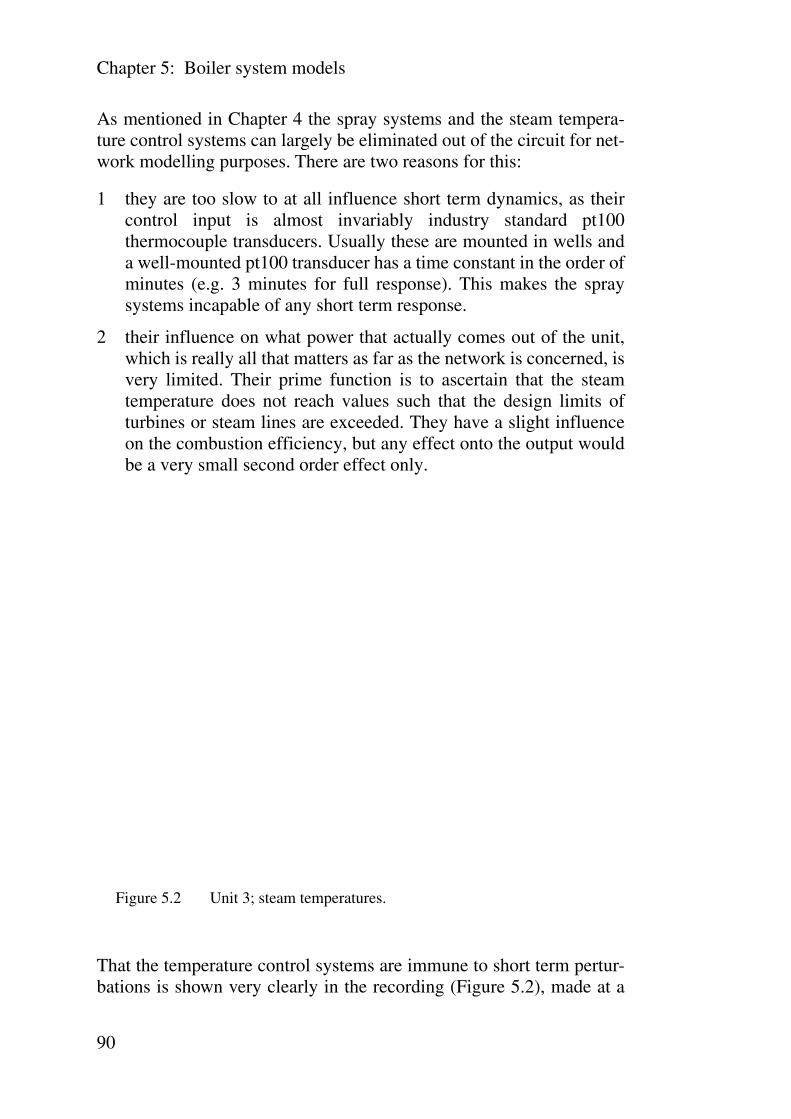
Chapter 5: Boiler system models
90
As mentioned in Chapter 4 the spray systems and the steam tempera-ture control systems can largely be eliminated out of the circuit for net-work modelling purposes. There are two reasons for this:
1 they are too slow to at all influence short term dynamics, as theircontrol input is almost invariably industry standard pt100thermocouple transducers. Usually these are mounted in wells anda well-mounted pt100 transducer has a time constant in the order ofminutes (e.g. 3 minutes for full response). This makes the spraysystems incapable of any short term response.
2 their influence on what power that actually comes out of the unit,which is really all that matters as far as the network is concerned, isvery limited. Their prime function is to ascertain that the steamtemperature does not reach values such that the design limits ofturbines or steam lines are exceeded. They have a slight influenceon the combustion efficiency, but any effect onto the output wouldbe a very small second order effect only.
Figure 5.2 Unit 3; steam temperatures.
That the temperature control systems are immune to short term pertur-bations is shown very clearly in the recording (Figure 5.2), made at a

Boiler system models
91
test on unit 3 at Stenungsund. Note that the temperatures were recordedusing the same pt100 temperature transducers as are used for the con-trol of the spray systems. This means that the recordings are identicalto the values used for the temperature control but not necessarily reflectthe true steam temperatures during the perturbation. If there were anyfast temperature changes these would have gone unnoticed.
It is obvious that the spray systems are not the ones responsible for anylack of temperature variations, as the temperature inputs that are theirinput control signals never change and thus these systems can take noaction.
5.5 Long term tests and models
Long term tests have not been performed within this project. There aretwo reasons for this: for power stations like the one at Stenungsund,with large steam storage volumes and valve control operation, longterm models are far less important as compared to the short termbehaviour, and also the units have not been available for such tests dueto their low usage. Stenungsund is primarily a backup/peak load stationand is in operation only a few days per year.
For other types of power stations, such as drum type boiler units, orany thermal power plants operating in sliding pressure mode, the longterm response is however highly interesting. As a continuation of thisproject it is therefore desirable that long term tests on such units can beperformed as well. Certain such tests can possibly also be done as sim-ulations against power station simulator units.
Certain long term models have been presented by E. Cheres [3]. Thesemodels are specifically designed for drum type boilers.

Chapter 5: Boiler system models
92

Composite models of entire power plants
93
Chapter 6 Composite models of entire power plants
This chapter deals with composite control models that can be substi-tuted for thermal power plants in network control studies and similar.The modelling is limited to units burning liquid or gaseous fuels, as thetests done as a part of this project gives no reference for models forplants burning solid fuels, where the response time of devices such ascoal milling or liquifying equipment, fuel conveyor systems have to betaken into account in case that the unit is operating in a sliding pressuremode. If however the unit operates in valve control mode with a suffi-ciently large steam accumulator and a sufficient pressure margin thenthese models will also be valid for units burning solid fuels, as theresponse time of the fuel cycle equipment will then be of no impor-tance with regard to the network behaviour of the unit.
Different level models will be discussed in the following, as the needvaries widely depending on what the model is to be used for. For manynetwork studies a very simple representation of the behaviour of apower station can be used, while certain special studies may require avery detailed and accurate model.
6.1 Units in valve control mode with sufficient steam storagecapacity
If it has been established, either through calculations as mentioned inChapter 5 or through measurements as discussed in Chapter 9, that fora specific unit the steam pressure can be kept up to its required valueeven when the unit taken on a load increase, i.e. that the steam storagecapacity is equal to or exceeds the boiler response time so that there isno pressure drop, then the boiler system and its associated subsystemscan be completely disregarded as far as the network response of theunit goes and only the turbine systems their associated control circuitryneed to be taken into account.
A simple model for this type of a unit will therefore be of the formshown in Figure 6.1.

Chapter 6: Composite models of entire power plants
94
Figure 6.1 Simple power plant model.
Some of these systems can clearly be seen in a typical response record-ing (Figure 6.2), this one being from a test of unit 4 at Stenungsund.
Figure 6.2 Unit 4; system response during a load increase. Note: Thisdiagram serves to illustrate the combination of events when theload is increased but does not, due to the gradual motion of thecontrol valve, allow for an exact determination of the responsetimes involved. For an indepth discussion, see Chapter 4.
Controlvalve limiter
Main controlvalve
Valve actuatordeadtime
Frequencycontrol system
Steamdome
Reheater +steamline delay
HP turbineresponse
MP+LP turbineresponse
Network frequency
Out
put p
ower

Composite models of entire power plants
95
Note that the fact that we have a control valve limiter makes theresponse of the power station unsymmetric: we have a limiter that canslow down the response to a load increase, but there is no correspond-ing limiter when the load is reduced. All other main components give amore or less symmetric response, with similar response characteristicswhether the load changes up or down. That the limiter in certain situa-tions have a considerable influence on the response of the unit isclearly shown by the example above. However, if we have a networksituation where the load changes that can be anticipated are not largeenough compared to the output power the control valve may never getinto contact with the limiter. This would for the system used at Ste-nungsund mean load changes less than 10% of the current outputpower. In such a situation the limiter can be eliminated out of the cir-cuit.
We have to make a distinction at this point as to which feedback varia-ble that is used. The choice of the feedback variable is, as was pointedout in Section 4.13, that important in influencing the response of theunit, especially when it comes to the initial response to a disturbance,that the same model can not be used for units that have a difference atthis point.
For a power station unit with a construction similar to that of the unitsat Stenungsund; i.e. where the feedback variable used is the controlvalve position and where a linearizer is used in the circuit control dia-gram for the model in Figure 6.1 gets the form shown in Figure 6.3.
In this model there are three input variables, whose values must bedecided on before the model is used for a simulation of some kind: 1)the steam pressure setting; which determines the power output for acertain valve opening and also gives the margin available in case ofoscillations etc. 2) the speed/power set point, which is normally opera-tor controlled and therefore normally constant in a short time perspec-tive and 3) actual network frequency, which in most studies of this kindwill be the input variable that we want to study the response to.
Note that any time delays in the high pressure turbine are neglected;i.e. the high pressure turbine output is modelled as instantly followingthe control valve position (for a given steam pressure).

Chapter 6: Composite models of entire power plants
96
Figure 6.3 Power plant model, neglecting the feedwater system powerconsumption. T1 is the time constant of the frequency controller.T2 is the time constant of the valve actuator. T3 is the deadtime ofthe valve actuator system. T4 is the time constant of the controlvalve limiter control system. TR is the deadtime of the reheaterand the medium pressure steam lines. TML is the time constant ofthe medium and low pressure turbine systems, including reheater and steam lines. C1, C2 are amplification factors. CH andCML are the amplification factors of the high pressure and themedium+ low pressure turbines respectively. These constantsgive the power ratio between the turbines.
6.2 Including the feedwater system
The model shown in Figure 6.3 can be extended to include the feedwa-ter system, or rather the power that is consumed by the feedwater sys-tem. This is the only aspect of the feedwater system that we need to
Steampressure Main control
valve actuator
1T2 · s
1T4 · s +
+
Control valve characteristics
Linearizer
T3
0.10
Valve actuatordeadtime
C2
–+
+Speed/power
set point–
1droop
T1 · s
1+T1 · s1+C1 ·
– Frequencyset point
+
Network frequency
TR
Deadtime
CML
1+TML · s
CHOutput
power

Composite models of entire power plants
97
consider here, as that is the only aspect in which this system influencesthe power output. The issue as to whether in a certain situation thefeedwater system may cause the unit to be tripped off the network isdealt with in Chapter 7. There are three main cases to be dealt withhere: 1) feedwater pump driven by a pump turbine, extracting steamfrom the medium pressure circuit; 2) feedwater pump driven by anelectric motor, with speed control through variable speed; 3) systemswith valve control of the feedwater flow. For a further discussion ofthese systems see Chapter 7.
Figure 6.4 Model including feedwater system power drain. Feedwatersystem powered by pump turbine using steam extracted from themedium pressure system. TF is the time delay of the feedwatersystem, including controller, pump turbine or electric motor,pump and water system. CF is a proportionality constant thatdepends on the amount of power used by the feedwater system.This constant is steam pressure dependant. In the case of valvecontrolled system this constant will have to be replaced by thepump characteristics, see above.
Steampressure Main control
valve actuator
1T2 · s
1T4 · s +
+
Control valve characteristics
Linearizer
T3
0.10
Valve actuatordeadtime
C2
–+
+Speed/power
set point–
1droop
T1 · s
1+T1 · s1+C1 ·
– Frequencyset point
+
Network frequency
TR
Deadtime
CML
1+TML · s
CHOutput
power
TF
Feedwatersystem delay
CF
+–
HP
stea
m f
low

Chapter 6: Composite models of entire power plants
98
Systems type 2) and 3) leads to the same block model, with the follow-ing differences: for units type 3) the time constant TF will be consider-ably shorter and CF will no longer be a simple proportionality constant,as the dependency of the power consumed on the feedwater flow willnow include the pump characteristics; i.e. how the power load of thepump will vary with the feedwater flow. Figure 6.5 shows a system oftype 2) as this kind is considerably more common than the valve con-trolled units.
With a simplified model of the feedwater system these different feed-water systems can be included in the power plant model as shown inFigures 6.4 and 6.5 respectively.
Figure 6.5 Model including feedwater system power drain. Feedwatersystem powered by electric motor with variable speed controlsystem.
Steampressure Main control
valve actuator
1T2 · s
1T4 · s +
+
Control valve characteristics
Linearizer
T3
0.10
Valve actuatordeadtime
C2
–+
+Speed/power
set point–
1droop
T1 · s
1+T1 · s1+C1 ·
– Frequencyset point
+
Network frequency
TR
Deadtime
CML
1+TML · s
CH
Outputpower
TF
Feedwatersystem delay
CF
+–
HP
stea
m f
low

Composite models of entire power plants
99
6.3 Simplified models
In most cases sudden load increases will not exceed 10%. The exactrepresentation of the control valve limiter may therefore be less impor-tant. If we eliminate the linearizer and the control valve characteristics,as these are basically set to equal out, as indicated in Section 4.12, weget a certain error in the signal controlling the control valve limiter, butwe get a much simpler model, and this one should be sufficient formost cases.
If we furthermore can conclude that most network load changes aregradual rather than instantaneous steps, then the deadtime of the con-trol valve actuator in the model can be eliminated. This one is verysmall: the control valve actuator deadtime is in the order of 0.2 to 0.3 s.This should be compared to the natural oscillation period times for thecase that the system becomes oscillatory. This time will of course varywith the moment of inertia of all machines that are synchronized ontothe network at each given time: the higher the moment of inertia thelonger the period of the oscillations. But even in the most extreme case,a single unit of the type like units 1 and 2 at Stenungsund, taking intoaccount that these units with their H value of just 2.2 are extremelylight machines, the oscillation period is in the order of 4 to 5 s and theactuator deadtime will then be in the order of 5% of the cycle time,which means it is not significant for the nature of the oscillations. It isof course, as mentioned in Section 4.14 highly important when one islooking at the inner control loop that is controlling the valve position,as here the cycle time is in the order of 1 s, but this is a control systemdesign problem and not relevant when it comes to the behaviour of theunit versus the network.
One must here assume that the inner control loop in this type of a cir-cuit, with its relationship between the actuator deadtime and the speedof the actuator, plus any integrating time delay that may have beenadded, is designed in such a manner that it is not self-oscillatory; i.e.any kind of order for a certain valve position must be executed withoutthat it gives rise to an oscillatory response.
A further simplification can be done by ignoring the reheater deadtimeTR and instead compensating for this by a small increase of themedium/low pressure turbine time constant TML.
Considering that the influence of the feedwater system is limited to afew percent this system is not represented in the simplified models.

Chapter 6: Composite models of entire power plants
100
With these simplifications we get a model of the type shown in Figure6.6.
Figure 6.6 Simplified power plant model.
A further simplification can be made IF the cases to be studied are suchthat there is no likeliness of the control valve limiter being activated.This will basically apply to all cases where no momentary powerincreases beyond a certain limit, usually about 10%, are to be expectedin the case that is to be studied. In such a case the limiter system canalso be eliminated. In cases where it is actually limiting the controlvalves motion the influence of the limiter can clearly not be ignored,but bearing in mind that in most networks the step load increases thatcan be expected tend to be below 5% this is a simplification that can bemade quite often.
Steampressure Main control
valve actuator
1T2 · s
1T4 · s +
+0.10
C2
–+
+Speed/power
set point–
1droop
T1 · s
1+T1 · s1+C1 ·
– Frequencyset point
+
Network frequency
CML
1+TML · s
CHOutput
power

Composite models of entire power plants
101
For this case we get a model of the type shown in Figure 6.7.
Figure 6.7 Simplified power plant model, no control valve limiter.
Steampressure Main control
valve actuator
1T2 · s
C2
–+
+Speed/power
set point–
1droop
T1 · s
1+T1 · s1+C1 ·
– Frequencyset point
+
Network frequency
CML
1+TML · s
CHOutput
power

Chapter 6: Composite models of entire power plants
102

Auxiliary systems of the power station
103
Chapter 7 Auxiliary systems of the power station
All power stations need certain auxiliary systems. In thermal powerstations these systems are quite extensive and of several differentkinds. The most important ones are the feedwater system, the fuel sys-tem and the firing fans. All these have a very direct influence on theboiler operation and a serious malfunction of any of these will mostlikely trip the boiler. Other systems may have a less direct position inthe chain leading to power output from the unit but are never the lessimportant; such as the condenser evacuation systems and the turbinelubrication system. There are also certain systems that are not at allpart of the power production units but that are still necessary in order toallow for proper operation of the power station; e.g. ventilation systemsto keep the temperature inside the station down to acceptable levels,environmental protection systems to make sure that the station com-plies with allowed operating limits for emissions etc.
In the case of a severe network disturbance or in a situation where thepower station is running in island operation on a small network thesedifferent systems may respond in different ways that may in somecases be less desirable. Where there is a marked influence of a particu-lar auxiliary system on the output power of the unit to the extent thatthe system has to be included in a network model of the power stationthen this has been dealt with in Chapters 4, 5 and 6. That aspect willtherefore not be in focus in this chapter. Instead there is another aspectwhich will have to be considered: can the auxiliary systems keep upwith e.g. large and rapid changes of the output power of the unit with-out that there is a risk that the entire unit trips due to the shortcomingof an auxiliary system. Almost all the auxiliary systems have the poten-tial to trip the unit if things go radically wrong and this risk must there-fore be investigated if one wants to get a correct picture of the ability ofa certain unit to operate under disturbed network conditions or in islandoperation mode on a small network.
7.1 The feedwater system
The feedwater system is the most high powered of all the auxiliary sys-tems and also the one that is likely to be the main restriction as for asthe auxiliary systems go when it comes to the ability of the unit towithstand perturbations. The proper operation of this system is abso-

Chapter 7: Auxiliary systems of the power station
104
lutely vital to the operation of the unit. The feedwater system must becontrolled in such a fashion that the amount of feedwater pressed intothe boiler at all times matches the amount of water leaving the boiler,either as steam or as water if any drains are used (most boilers are oper-ated with a certain small drain from the bottom of the steam dome inorder to reduce the amount of impurities present in the steam and in thewater). If this balance can not be kept up accurately then the waterlevel of the boiler system and the steam dome will change. If thesechanges go outside of certain quite tight limits the boiler, and hence theentire unit, is tripped.
Many different designs are possible when it comes to the feedwatercontrol. The oldest kind is to use valve control on the feedwater itself;just regulate the flow by controlling the valve, whereas the feedwaterpumps run at full speed all the time. This control mode does allow forquite fast response in the case of disturbances or rapid changes of theoutput power of the unit, but is clearly uneconomical, as the feedwaterpumps have to be run at full power at all times, whether the actuallydemand for feedwater would require that amount of pump power ornot. This means higher losses and increased costs. As the feedwatersystem, as was mentioned above, is very high powered these costs maybe quite substantial. It is normal for the feedwater pumps to consumein the order of three to five percent of the output power of the unit andthis is high enough to make economical operation of the feedwater sys-tem an important issue.
Another mode of control is used in stations like the one at Stenung-sund, where the feedwater pumps are steam powered, with their ownpump turbines. In this case the feedwater flow rate can be controlled byvalve controlling the steam flow rate to the pump turbines and hencethe speed of the turbines and the pumps. This type of valve controlshow considerably lower losses but it has the drawback that there is anadditional delay built into the system: if there is a change in thedemand for feedwater both the control valve and the pump turbines andthe pumps themselves have to respond and the response time is there-fore comparatively long. Later on in this section we will look at the dif-ficulties that this can lead to.
If the feedwater pumps are driven by electric motors rather then bysteam turbines then there are basically three ways of controlling thefeedwater flow: the old way with a valve directly on the feedwater,pump speed control by the means of a variable coupling and pumpspeed control by means of controlling the electric motors themselves,

Auxiliary systems of the power station
105
either by the use of DC drives or by the use of frequency converters.The former is expensive, as DC motor systems are expensive both topurchase and to operate. The latter is a promising method that maywell be more commonly used as the price of the necessary frequencyconverters is gradually going down. So far this method have not beenused much, due to the high price of the converters.
The variable coupling method is in common use and allows for a rea-sonable economy. There are losses involved, but these are clearly lowerthen for valve feedwater control. The response is unfortunately notvery fast, as just in the case with the steam turbine pump systems, thepump has to be regulated first and only after that will we see any con-trol influence unto the feedwater flow rate itself. The response time willtherefore be similar in order to that of the pump turbines with steamvalve control. Due to its common use this type of feedwater control isthe one used for most power station models, including the IEEE stand-ard models.
The various types of feedwater systems are shown in Figure 7.1-7.5.
Figure 7.1 Basic valve control.
Figure 7.2 Pump turbine with turbine speed control.
M
to boilerpumpfeedwater
electric motor(no speed control)
controlvalve
to boilerpumpfeedwater
steam input
steam control valve
pump turbine

Chapter 7: Auxiliary systems of the power station
106
Figure 7.3 Electric drive with variable speed coupling.
Figure 7.4 DC motor drive system.
Figure 7.5 Variable frequency drive system.
The Stenungsund power station is equipped with steam turbine drivenfeedwater pumps and the feedwater is for low power operation control-led by a valve and for medium and high power by controlling the speedof the pump turbine, using a steam control valve. Electric feedwater
M
to boilerpumpfeedwater
electric motor(no speed control)
variablecoupling
M
to boilerpumpfeedwater
DC motor
SCRrectifier
M
to boilerpumpfeedwater
AC motor
Frequencyconverter

Auxiliary systems of the power station
107
pumps are available as backups. These are used only if the pump tur-bine or its pump is for some reason not available and operation usingthe backup pump does not allow for running the units at full power.E.g. for units 3 and 4 the power has to be reduced from 260 MW to 160MW in such a case. If the electric pumps are in use feedwater control isachieved by a control valve on the feedwater line.
As for the feedwater control system there are many different designs aswell, but the basic principle of operation tends to be the same. The sys-tem shown below is for the units at Stenungsund, but similar types ofsystems are used almost universally. The steam flow rate of the highpressure steam line is the main control variable for this system. Thesecond variable is the dome level, as was briefly discussed in Chapter4. The control system outlay is shown in Figure 7.6.
Figure 7.6 Stenungsund power station, Units 3 & 4, Feedwater controlsystem.
When the different tests were done on the units at Stenungsund thefeedwater system mostly responded reasonably well, but there was amarked delay which could cause trouble if the perturbations during asevere network disturbance got serious enough, or if the unit duringisland operation on a very small network should come into an oscilla-tory mode with large variations in the output power.
The problem involved comes from the time delay between the changeof the HP steam flow rate and the actual change of the feedwater flowrate. This delay turned out to be of the same order as the period ofoscillations that could sometimes occur when the unit was operating ona network all alone; i.e. with only the moment of inertia of the unititself present on the network. In such a case the feedwater system could
+
–+
++
–
Dome level set point
Dome level
HP steam level
Feedwater flow
Signal to pump
turbine controller
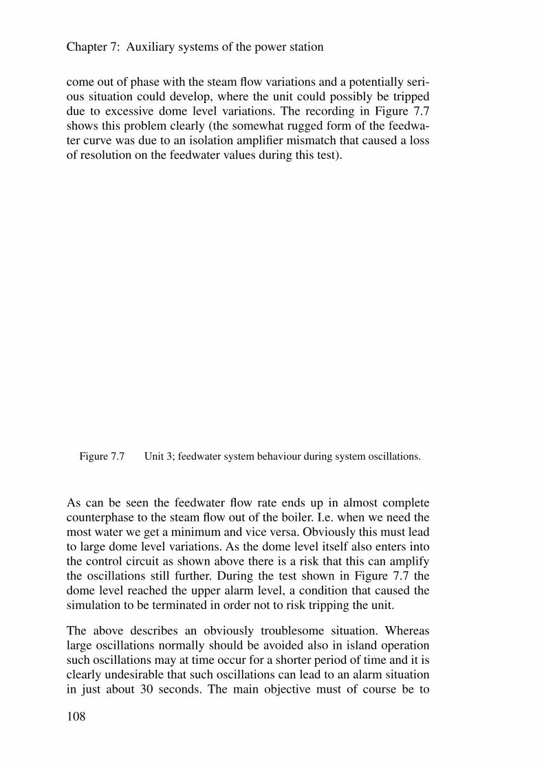
Chapter 7: Auxiliary systems of the power station
108
come out of phase with the steam flow variations and a potentially seri-ous situation could develop, where the unit could possibly be trippeddue to excessive dome level variations. The recording in Figure 7.7shows this problem clearly (the somewhat rugged form of the feedwa-ter curve was due to an isolation amplifier mismatch that caused a lossof resolution on the feedwater values during this test).
Figure 7.7 Unit 3; feedwater system behaviour during system oscillations.
As can be seen the feedwater flow rate ends up in almost completecounterphase to the steam flow out of the boiler. I.e. when we need themost water we get a minimum and vice versa. Obviously this must leadto large dome level variations. As the dome level itself also enters intothe control circuit as shown above there is a risk that this can amplifythe oscillations still further. During the test shown in Figure 7.7 thedome level reached the upper alarm level, a condition that caused thesimulation to be terminated in order not to risk tripping the unit.
The above describes an obviously troublesome situation. Whereaslarge oscillations normally should be avoided also in island operationsuch oscillations may at time occur for a shorter period of time and it isclearly undesirable that such oscillations can lead to an alarm situationin just about 30 seconds. The main objective must of course be to

Auxiliary systems of the power station
109
adjust the main frequency control system parameters in such a way thatany such oscillations are damped much more rapidly, but a higher levelof tolerance against oscillations on the part of the feedwater systemwould also be of a clear advantage.
An obvious way of getting the feedwater system to better track thesteam flow would of course be to speed up the response of the feedwa-ter system. This is however very difficult to do. The response time ismostly a function of the physical design of the systems and whereas itmay be possible to have this in mind when constructing a new powerstation it can not be made as a retrofit, at least not without excessivecosts. The only parameters we can control will therefore normally bethe settings of the feedwater controller: the balance between the influ-ence of the steam flow versus that of the dome level and the normalcontroller settings such as gain and integration time. One can of coursealso add a reasonable portion of derivative action, but this must be donewith great care, as too much derivative action is likely to make the con-trol system unstable. Another option is, unless the unit normally usesvalve control, to temporarily switch to such a mode when the unitundertakes tasks like island operation on a small network.
Virtually all units do have a control valve, also if the prime mode ofcontrol is something else than valve control. The reason for this is thata feedwater pump system can not operate at very low speeds. The pres-sure generated drops by the square of the pump speed and would for avery slow-running pump be too low to overcome the boiler pressure, inaddition to that speed controlled pumps often show tendencies of insta-bility if the speed gets too low. Normally a pump of this type is notoperated below approximately half of its rated speed, and for lowpower operation there is always a control valve fitted. Provided thatone has verified that the pump system and the valve can stand this itcould be possible to switch to valve control mode manually when theunit is operated in extreme operation modes where the feedwater con-trol may need to respond faster than what it does normally. Such achange of control mode will of course be at the expense of efficiency,but that is hardly a prime consideration during emergency operationwhere the main matter is to make sure that the unit survives on the net-work.

Chapter 7: Auxiliary systems of the power station
110
7.2 Fuel system
The fuel system response characteristics are usually of importance onlyfor units running in sliding pressure operation or for units where thesteam storage capacity is comparatively low so that a fast response onthe part of the fuel control system and the boiler is required in order totake on a load increase without a drop in the boiler steam pressure. Incertain situations there can however be a risk of resonance phenomenadue to the inherent control loop delays and in such cases a furtherinvestigation may be necessary.
In the case of sliding pressure operation the response time is usually,even with the fastest of fuel control systems, too slow to allow the unitto perform frequency control duties on a very small network. Typicaltime constants are in the order of several hundred seconds, which inturn requires either a fairly large network or that there are other, faster,units on the network that can take care of the necessary fast initialresponse in the case of a large change of the network load.
For units operating in sliding pressure mode the fuel control is inte-grated into the output power control system; i.e. the frequency controlsystem if the unit is performing frequency control. For other units thereare usually three basic control modes that can be used for fuel control:dome pressure regulation, power output tracking and manual control(fixed firing). Dome pressure regulation is a quite safe and basic form.In this case there is hardly any risk of resonance problems and the con-trol system should, if correctly designed, be stable under all operatingconditions. The drawback is a somewhat slower response: the systemwill not respond to a load change until there has been an actual changeof the dome pressure, and as a result there would be constant up/downvariations of the dome pressure, which causes increased wear and riskfor metal fatigue. Instead most systems are designed to also track theoutput power, so that the firing is adjusted immediately when the out-put power is changed. This means a faster response, but also a certainrisk for instability or resonance.The control system will basically bedesigned as in Figure 7.8.

Auxiliary systems of the power station
111
Figure 7.8 Basic fuel control system based on steam flow and dome pressure.
The tests run at the Stenungsund power station showed that the fuelcontrol system tracked the steam flow, and hence the power output,quite well, though with a delay in the order of 6 seconds. A typicalresponse is shown in Figure 7.9. As can be seen there are considerableoscillations at one point and such oscillations could be observed at sev-eral times, always following a reduction of the fuel rate. It seems toindicate some kind of instability in the fuel control system that couldwarrant further investigation.
An oscillation in the fuel supply rate is undesirable from several pointsof view. One is that it produces unnecessary thermal/mechanical strainon the boiler as the temperature varies. Another one is that it may leadto improper combustion and increased emissions. One should note thatdue to the time delay of the firing fan system the air supply to the com-bustion does not vary when the fuel supply oscillates in this manner.That must inevitably lead to that some of this combustion is done at anon-optimum fuel/air mix ratio and hence to a degradation of the com-bustion.
It should be noted that the developed test method with step-wise loadchanges is very suitable for detecting these kind of problems. No spe-cial test was made to check the fuel system, instead the above could be
–+
Dome pressureset point
Dome pressure
HP steamflow
Pressure deviation
To fuel control valves
C1 · sPressure tendency
C2
Steam/fuel ratio set point
+
+
–
–

Chapter 7: Auxiliary systems of the power station
112
observed when analysing the results from a general test run of the unitconnected to the simulator system. As all main control systems get ver-ified at the same time valuable time is saved when it comes to the needfor using the actual unit for testing.
Figure 7.9 Fuel system response.
7.3 Combustion airflow control
The combustion airflow control is directly linked to the fuel controlsystem. In most cases it is based on a ratio air to fuel, but certain otherinput signals may be added as well. In the case of the Stenungsundpower station, units 3 and 4, there is a special connection to the steamflow rate, which will add extra air in case of a steam flow increase. Thereason for this is to avoid incomplete combustion due to a shortage ofair if there is an increase in the steam flow: the increased steam flowwill soon be followed by an increase in the fuel flow rate and if the air-flow is not increased accordingly we get a combustion with a shortageof air and hence a black puff of smoke may be discharged to the envi-ronment. By letting the steam flow influence the airflow one can ascer-tain that the increase of the airflow comes a little ahead of the increased
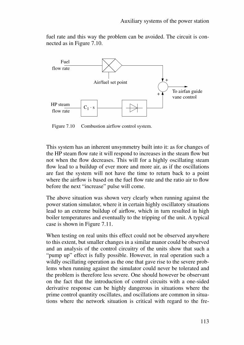
Auxiliary systems of the power station
113
fuel rate and this way the problem can be avoided. The circuit is con-nected as in Figure 7.10.
Figure 7.10 Combustion airflow control system.
This system has an inherent unsymmetry built into it: as for changes ofthe HP steam flow rate it will respond to increases in the steam flow butnot when the flow decreases. This will for a highly oscillating steamflow lead to a buildup of ever more and more air, as if the oscillationsare fast the system will not have the time to return back to a pointwhere the airflow is based on the fuel flow rate and the ratio air to flowbefore the next “increase” pulse will come.
The above situation was shown very clearly when running against thepower station simulator, where it in certain highly oscillatory situationslead to an extreme buildup of airflow, which in turn resulted in highboiler temperatures and eventually to the tripping of the unit. A typicalcase is shown in Figure 7.11.
When testing on real units this effect could not be observed anywhereto this extent, but smaller changes in a similar manor could be observedand an analysis of the control circuitry of the units show that such a“pump up” effect is fully possible. However, in real operation such awildly oscillating operation as the one that gave rise to the severe prob-lems when running against the simulator could never be tolerated andthe problem is therefore less severe. One should however be observanton the fact that the introduction of control circuits with a one-sidedderivative response can be highly dangerous in situations where theprime control quantity oscillates, and oscillations are common in situa-tions where the network situation is critical with regard to the fre-
HP steamflow rate
To airfan guide vane control
C1 · s
Air/fuel set point +
+
Fuelflow rate

Chapter 7: Auxiliary systems of the power station
114
quency control capability of the units responsible for maintaining thenetwork frequency.
Figure 7.11 Simulator run with large oscillations and automatic fan controlincreasing the combustion airflow out of control.
Load shedding
Network frequency
Output power
% MW Hz
300
200
5251
50
010
2030
4050
6070
8090
100
100
0
4948
0 50 100 150 200 sTime
m3/s%1 %2
400
300
200
100
0
100
8060
2015
105
0-5
-10
-15
-20
4020
0
0 50 100Time
150 200 s
Combustion airflow
Air fan guide vane position(scale 2)
air controller deviation(scale 1)
unit is tripped dueto high superheatertemperature

Island operation. Problems, prerequesites and operating recommenda-
115
Chapter 8 Island operation. Problems, prerequesites and operating recommendations
Island operation is normally used to refer to a situation where a nor-mally interconnected larger network has been subdivided into smallernetworks that operate as autonomous islands, with no connection inbetween these islands. Networks that are designed to be operated sepa-rately, like on a group of real physical islands are not included in thisterminology, although some of the problems would be identical. How-ever, this latter situation is normally easier to manage, as all controlsystems would then be specifically designed for this kind of a system.
A power station running on a larger interconnected network can end upin island operation in basically two ways. One is intentionally if thenetwork has crashed for some reason and there are such problems (e.g.serious damage to main network components) that the main networkcan not be brought up again within a reasonable amount of time. Insuch a situation one may decide that one has to start up island systemswherever possible in order to be able to resume deliveries to as manycustomers as possible. The other possible way is that in interconnectednetwork inadvertently breaks up into smaller islands as a result of seri-ous faults on the network; like the tripping of main transmission linesor interties, loss of synchronism between different parts of the networketc.
There are several different problems that can cause serious difficultieswhen a power network is forced into island operation. The most seriousones are linked to maintaining correct network frequency and in regu-lating the network voltage. Especially the frequency can be cumber-some, as the total moment of inertia in the system is quite small andany imbalance between the power produced and the power consumedby the loads will therefore quickly lead to a shift in network frequency.In addition the power stations available for frequency control purposesmay not be very well suited for frequency control; either because oftheir design or because control system settings are only optimized foroperation on the interconnected network. In many cases these stationsnever perform any frequency control duties at all in normal operationand hence the frequency control systems are not properly tested and thestations operators are also neither trained for it or experienced in thismode of operation.

Chapter 8: Island operation. Problems, prerequesites and operating
116
As shown in Chapter 3 the total moment of inertia is of great impor-tance when it comes to the behaviour of a power plant when it is inisland operation. The higher the moment of inertia, the better the stabil-ity and the smaller the oscillations and frequency deviations that occurwhen there are transients. This effect is an obvious result of the swingequation that governs the dynamic behaviour of the network:
(8.1)
where: J is the total moment of inertia present in the system
ω is the angular velocity of the system
∆P is the difference at the given time between the total powerproduced within the network and the power consumed(including system losses)
As the frequency of the network is directly proportional to ω:
(8.2)
where: f is the network frequency; we see that the rate at which thefrequency will change for a given change in the load P isdirectly proportional to the total moment of inertia J.
8.1 Moment of inertia considerations
As shown in Chapter 3 the difference of e.g. running a single unit andthat of running four units (all units at the Stenungsund station) is suffi-cient to make the difference between smooth operation and a moreoscillatory behaviour.
The moment of inertia of a certain power station unit is a designparameter and can of course not be altered afterwards by any reasona-ble measures. However, one can influence the moment of inertiapresent on the network by the strategy used in dispatching of the units.Taking again the Stenungsund power station as an example; if the sta-tion is to supply a total of 200 MW to a small local island network thiscan be done using a single unit, if one of the two larger units is used(260 MW capacity each). However, the same power can also be deliv-ered by both these units operating in parallel at 100 MW each. In the
tdd 1
2--- J ω2⋅ ⋅
∆P=
ω 2 π f⋅ ⋅=
Island operation. Problems, prerequesites and operating recommenda-
117
latter case the moment of inertia is twice as high and this will then givea significant improvement to the stability of the network. It will meansomewhat higher costs, as the efficiency of a power station unit is usu-ally somewhat less at operation down as low as below 50% of its ratedcapacity, plus that it is likely that more operators will be needed inorder to run the two units, but cost efficiency is hardly a main concernin an emergency situation where the survival of the network is thenumber one consideration.
It is a major advantage of the test and simulation method developedwithin this project that the behaviour of a power station unit in opera-tion on networks with different levels of moment of inertia can veryeasily be tested. The J value can even be changed by a simple com-mand in the middle of a simulation and it is thus easy to verify howmuch moment of inertia that is required in order to obtain a stableoperation with regard to the network frequency control.
8.2 The importance of the droop value
An other parameter of main concern is the droop. The droop is in thepower industry perhaps mainly thought of as a control deviation that isnecessary in order to distribute the load changes in correct proportionsunto different units that operate in parallel on the same network. This isbecause the load changes are distributed in inverse proportion to thedroop of the units. Thus, if a unit has a low droop value it will be takingon a large proportion of load changes on the network. On the otherhand, a unit with a high droop value will be less active when it comesto participating in the network frequency control, in that its response tochanges of frequency will be much smaller. With very low droop val-ues successful parallel operation becomes impossible, as the slightestchange in frequency will produce large changes in output power andeven differences in frequency set points will have severe influences. Asimple figure can illustrate this far the case of only two units operatingonto the same island network.
Figure 8.1 shows how two units in parallel respond to a load increase inthe network. As can be seen unit 2 has a lower droop (lower inclinationof the frequency/power curve) and will take on a larger part of thepower increase than will unit 1.
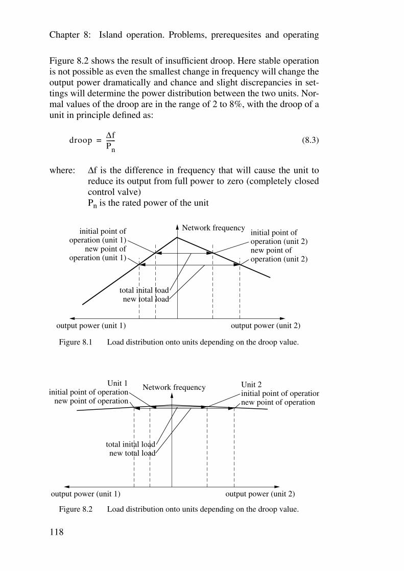
Chapter 8: Island operation. Problems, prerequesites and operating
118
Figure 8.2 shows the result of insufficient droop. Here stable operationis not possible as even the smallest change in frequency will change theoutput power dramatically and chance and slight discrepancies in set-tings will determine the power distribution between the two units. Nor-mal values of the droop are in the range of 2 to 8%, with the droop of aunit in principle defined as:
(8.3)
where: ∆f is the difference in frequency that will cause the unit toreduce its output from full power to zero (completely closedcontrol valve)Pn is the rated power of the unit
Figure 8.1 Load distribution onto units depending on the droop value.
Figure 8.2 Load distribution onto units depending on the droop value.
droop ∆fPn------=
Network frequency
output power (unit 2)output power (unit 1)
initial point ofoperation (unit 1)
new point ofoperation (unit 1)
total inital loadnew total load
initial point ofoperation (unit 2)new point ofoperation (unit 2)
Network frequency
output power (unit 2)output power (unit 1)
Unit 1initial point of operation
new point of operation
total inital loadnew total load
Unit 2initial point of operationnew point of operation

Island operation. Problems, prerequesites and operating recommenda-
119
The droop value does however for very small networks also haveanother impact than on the load distribution, namely on the control sta-bility of the unit and on its tendency to oscillate before settling to a newload level when the network is subjected to a sudden load change.Comparisons between the tests at the Stenungsund power station onunit 4 with 8% droop and unit 3 with 4% droop, as shown in Chapter 3,show clearly that the operation becomes much more stable and theresponse much less oscillatory when a higher droop setting is used.This is natural, as the droop actually enters into the control loop as anamplification factor and higher amplification factors will normally leadto more accurate but less stable control, with an oscillatory response, orin the extreme case with amplification factors way beyond the allowa-ble, to a self-oscillating behaviour. A very simple control loop for theunit and the network can be thought of as in Figure 8.3.
Figure 8.3 Frequency regulation control loop.
The above shows that in the case of island operation higher droop val-ues may be desired, as compared to normal network operation. Thiswill prevent oscillations and will provide for a smoother regulation.This will of course be at the expense of frequency correctness, but thisshould hardly be a main concern in an emergency operating situation,where absolute frequency correctness is hard to achieve anyhow andwhere problems with e.g. synchronous clocks must be considered ofsecondary importance only. Most industrial and domestic loads canhandle frequency variations of up to ±5% without any major change intheir mode of operation and this gives very free limits compared to the
+–
PID-circuit turbinecontroller front end
1droop
Valve positioncontrol loop
Turbinesystem response
Network response(swing equation)
NetworkloadPower balance
offset
Valve position
Power output
Net
wor
k fr
eque
ncy

Chapter 8: Island operation. Problems, prerequesites and operating
120
extreme accurateness that is normally kept when it comes to maintain-ing the network frequency.
However, there are other factors that also set an upper limit for thedroop value. One such factor, which was mentioned in Chapter 4, isthat with a high droop value we get a lower value of the load reductionthat the unit can handle without that the intercept valves are activated.This must clearly be avoided and either the droop value has to be keptlow enough to prevent operation of the intercept valves, or the stationoperators must closely monitor the load changes and adjust thespeed/power settings accordingly, so that the point of operation used bythe automatic frequency control system is close enough to the nominalfrequency to prevent this. Note that the latter possibility exists only ifeither one power station is alone on the network or if there is a wellplanned and properly functioning central load dispatch centre that canundertake to coordinate different units on the network in this respect(secondary frequency control schemes).
8.3 Load distribution based on the speed of response
If we go by the droop value of the units that are on line in a small islandnetwork it should be easy to predict how a change of the load levelwould be distributed between the different units. However, one mustbear in mind that the droop value as a measure for the distribution ofthe load is only valid once that all units have reached a new equilibriumstate. Before that happens it will be the speed of response of the differ-ent units and not the droop that will be the key factor in determininghow the load is distributed. If different types of production units are online on the network then there may well be very substantial differencesin the speed of response and this can definitely not be ignored when thebehaviour of the network is discussed. As an example, a unit with ahigh droop value but a very fast response will initially take on muchmore than its share when a load increase hits the system. Eventually,when the other slower units catch up, it will then return down to theload level that is determined by the droop value of the units.
This fact may mean that a unit with a fast response will get more loadthan what it can handle, at least for a short period of time. In this kindof a situation the control valve limiter is highly important. It serves toprevent the unit from taking on more load than allowable, but oneshould note that this is of course done at the expense of frequency cor-
Island operation. Problems, prerequesites and operating recommenda-
121
rectness: it will clearly take longer for the system to get out of the fre-quency dip that a sudden load increase creates as compared to if therewas no limiter and the fast unit would be allowed to take on a higherload right away.
8.4 Mixed sources of production
If the production resources available on a small island network are ofdifferent types; e.g. thermal and hydro power or thermal units withvalve control plus units with sliding pressure operation then it is clearlyhighly important to take this into account when planning for such anisland operation mode. The very different speeds of response will, asindicated above, be of great importance when it comes to the instanta-neous load distribution and this can prove both a problem and a condi-tion that can be used to advantage.
It is generally believed in the power industry that if hydro power isavailable for frequency control purposes then that should be given thattask whereas thermal units should only be used for frequency controlwhen there is no other alternative. This may perhaps not always betrue. It is undoubtedly so that hydro electric power stations are veryreliable for control purposes and that they are also very rugged, in thatit is possible to change the output power up or down without concernfor temperature gradients, risk for a reduction of component lifespanetc., and in a normal network with a reasonably large moment of inertiathe frequency can be kept very accurately at the desired value using thehydro units governor systems. However, hydro units have one draw-back that is normally not thought of: they are fairly slow compared tothe control characteristics of the steam turbine systems. In a very smallnetwork, where there is only very limited moment of inertia availableand where the frequency changes very rapidly in case of a sudden loadchange this may be highly important.
As the tests made within this project show thermal power units can beextremely fast. The the control valve moves in fractions of a secondand the high pressure system responds almost instantaneously. Forhydro units the response is much slower. It takes several seconds forthe guide vane control system to move the vanes, water has to be accel-erated etc. In some cases extremely slow governor systems have to beused because of the hydraulic conditions; this is the case where suddenincreases in the flow of water could lead to severe erosion of riverbanks

Chapter 8: Island operation. Problems, prerequesites and operating
122
and similar. In such cases the restrictions of the allowed rate ofincrease of the water flow and hence of the power output may be verystringent.
With a suitable mix of units and suitable control settings it should befully possible to use this to achieve a more optimized frequency controlof an island network. Suppose for instance that we have a thermal unitplus a hydro unit as the two sole supplier to the network. If we set theresponse of the thermal unit as fast as possible (no additional inten-tional delays, apart from what is required in order to make internal con-trol loops stable etc.) and give that unit a large droop setting and givethe hydro unit a much lower droop setting we will get the followingresponse to a load increase: the thermal unit will respond almostinstantaneously. Provided that the unit has a reasonable steam storage,either through a dome or in the steam generators, then there is no needto wait for an increase in the firing. After a number of seconds thehydro unit will respond. As it has a lower droop value it will take on thebulk of the load increase and relieve the thermal unit of any substantialchange in the firing and thus of additional strain and wear on the boilersystems. We then get the very fast response of the steam turbine systemand at the same time the rugged reliability of the hydro system.
A typical example is shown in the two simulations shown in Figures8.4 and 8.5. These are simulations that were done using the models dis-cussed in Chapter 6. Two sources of production were considered. Oneis a 300 MW unit of a type similar to the large units at Stenungsund,nominal power of 300 MW, time constants similar to those of the Ste-nungsund units (4.5 s reheater/steam line delay) and using the simpli-fied model of Figure 6.6. The other unit is assumed to be a slow hydrounit, with a governor motion time constant of 25 s, using the samemodel but with the medium/low pressure part taken out, as we nowhave only one turbine, namely the water turbine.
In the first simulation the thermal unit was given a droop of 8% and thehydro unit 2%. Normally this would mean that a greater portion of theload would be taken care of by the hydro unit, but because of the differ-ence in the speed of response the thermal unit helps out more than itsshare initially. The test is for a step load increase from 200 MW to 220MW on the network, with just these two units being on the networkand with an assumed total moment of inertia of 0.045 . 106 kgm2,which should be a fairly normal value for this type of a combination.

Island operation. Problems, prerequesites and operating recommenda-
123
The frequency is rapidly restored and the network does not receive anymajor disturbance. We see here that the thermal unit takes on a largerportion of the load for a period of about 5 s, until the slower hydro unitcatches up and allows for the thermal unit to reduce its output. Itshould be noted that this kind of a power boost can be done withoutany additional thermal stress onto the thermal unit, as with proper con-trol settings there is no need to increase the firing for this extra boost,as the steam stored in the dome or the steam generators will for mostdesigns of thermal units be sufficient.
Figure 8.4 Thermal and a hydro unit sharing the responsability for thefrequency control.
If instead we run the same simulation, with the same controller set-tings, but with what would be a more conventional dispatch strategy:the thermal unit running a fixed base load and the hydro unit alonebeing responsible for the frequency control, we get a totally differentresponse. The frequency dip on the network gets far more severe and inaddition we have large oscillations that are only slowly damped. Thecontroller settings were in this case not optimized for the hydro unitand with another set of control system settings these oscillations couldmaybe be prevented or reduced, but the large initial frequency dip
49.0
50.0
51.0
025
5075
100
125
150
175
025
5075
Hz MWMW
output power, thermal unit
output power, hydro unit
network frequency
0 5 10 15 20 sTime

Chapter 8: Island operation. Problems, prerequesites and operating
124
could not. It is a direct consequence of the slow response of the unitresponsible for maintaining the frequency. (note that the time scale isdifferent from that of Figure 8.4).
The above example shows clearly that when it comes to island opera-tion on a limited network each case has to be studied carefully andwithout prejudices with regard to one kind of power stations being gen-erally more suited for frequency control purposes compared to another.
Figure 8.5 As in Figure 8.4 but with the thermal unit running with constantpower.
If island operation in accordance with the principles mentioned aboveof a certain area is being planned as part of e.g. making up emergencypower distribution plans then the test method developed in this projectis an excellent tool to test and verify the operation. The simulator sys-tem can then be connected to the thermal unit and the hydro units canbe included in the network description that is fed to the simulator sys-tem prior to a test. As the hydro units due to their simplicity can fairlyeasily be modelled quite accurately this is a quite easy way of testingthe cooperation between the different units and making certain e.g. thatthere are no stability problems in the system e.g. as a result of thecooperation of control systems with completely different characteris-tics.
49.0
50.0
51.0
025
5075
100
125
150
175
025
5075
Hz MWMW
output power, thermal unit
output power, hydro unit
network frequency
0 5 10 15 20 sTime
25 30 35 40 45 50

Island operation. Problems, prerequesites and operating recommenda-
125
8.5 Operating recommendations
Obviously the operating recommendations will be quite different foroperation on an island network, as compared to operating on a large,normal one.
One clear difference is that the trade-off between control reliability andthe economy of operation will be very different in an emergency situa-tion where supplying power to the network is the main and almost theonly concern. A typical consequence of this is to maintain a higherdome pressure compared to the point of operation than what wouldnormally be used. Keeping a higher steam pressure means a larger mar-gin in case of perturbations or sudden load increases, but also meanshigher losses and a somewhat lower overall efficiency.
Another such consequence is that one must operate the units, at leastthose responsible for the frequency control, with a lower output power.This serves to achieve stable operation and to ascertain that there isenough additional power available in the case of a sudden load increaseor if a unit of production is tripped. As pointed out earlier it can e.g. bebetter to run two 250 MW units at 100 MW each rather then running200 MW on one unit.
If control stability of the fuel control is a problem it may be moreadvantageous to change to manual fuel control in a situation of thistype.
Certain protection systems may also need to be changed. A typicalexample is the fuel/output power differential protection system thatsome units are fitted with. Such systems are designed to operate in caseof e.g. excessive amounts of water in the fuel or similar, but they arenot vital to the safety of the unit and there is always an inherent riskthat they can trip the unit if there are large perturbations. This hap-pened several times when running tests against the Stenungsund powerstation simulator. It may therefore be recommendable to set systemslike these to signal only (no tripping) for emergency operation on smallisland networks, where large perturbations are more likely then whenthe unit is in normal operation.
It may be tempting to put many of these suggestions into the program-ming for a computer controlled control system. A special set of settingsfor emergency operation can then be set up and the switching to suchemergency operation can then be done at the touch of a button or even

Chapter 8: Island operation. Problems, prerequesites and operating
126
automatically upon certain network behaviour conditions. This may bequite recommendable but it should be done with due caution, so that itdoes not put severe restraints on what the station operators can do man-ually. Emergencies are always unpredictable and the way a certainemergency will develop can not always be accurately predicted. Stationoperators with a long experience often know every part of the behav-iour of their station very well and can often find ways to improvisetheir way through situations that were not thought of when the auto-matic control system was programmed. A possibility for the operatorsto do certain things manually in the case of emergency may often bethe difference between being able to handle an extreme and unforeseensituation and getting tripped off the network.

Recommended test procedures for testing power plants
127
Chapter 9 Recommended test procedures for testing power plants
The test system and method that has been developed within this projectallow for the testing of power station units, e.g. with regard to theirbehaviour in island operation, while they are still synchronized ontothe normal network. In order to use these possibilities to their fullcapacity any tests that are run should be carefully planned so that max-imum information can be extracted from the results. This is of courseespecially true for units that are only rarely in operation and where theavailability of the unit for testing may be a major limitation.
9.1 Connecting a unit for testing
Before a unit can be tested using this method one must of course makesure that proper connections to the unit can be made. There are onlytwo connections that are absolutely required if a test of this kind shouldbe possible: an output signal from the unit which is a measure of thetotal electric power (active power) that is being delivered to the net-work and an input signal to the unit that takes the place of the normalnetwork frequency input that is supplied to the frequency control sys-tem.
The output power measurement is normally the easiest one to connect.In most cases there is some signal transducer that outputs a signal pro-portional to the output power, often on a 0–20, 0–50 or 4–20 mA cur-rent loop base. Such a signal can easily be transferred, normally via anisolation amplifier in order to maintain galvanic separation, to themeasurement system of the simulator. For some older units the outputpower may not be directly available, as the meter that shows the outputpower is directly connected to the PTs and the CTs of the unit. In sucha case a separate transducer may have to be mounted for the tests.
The input to the frequency control system may have to be done in dif-ferent ways depending on how the frequency control system of the unitis constructed. The most common is for older units that the signal usedcomes from a tachometer generator connected directly to the turbineshaft. This signal is then normally converted to a DC signal in someway. On older units this is done using discriminator circuitry, on newer

Chapter 9: Recommended test procedures for testing power plants
128
ones through various electronic circuits. This signal chain can then beinterrupted in different ways in order to allow for an external signal tobe input. In some cases this can be done very easily as some turbinecontrollers are fitted with a separate test input.
More modern units may often have speed transducers rather then tachogenerators as their speed input source. These are often built for output-ting a low level DC signal that can be easily intercepted. Some of themost modern constructions use digital transducers, in which case thetransfer of information must be done by computer communicationmeans.
Figure 9.1 AC connection.
Figure 9.2 DC connections.
G
tacho generator
changeoverrelay
frequencycontrol system
simulator
AC signal
G
tacho generator
changeoverrelay
frequencycontrol system
simulator
AC signal
discriminatoror f/v converter
DC signal, e.g. -10 - +10 V
changeoverrelay
frequencycontrol system
simulator
DC signal
speedtransducer
a)
b)

Recommended test procedures for testing power plants
129
Figure 9.3 Digital connection.
Where connection to a low level DC input or a digital input can bemade this is always preferable, as using AC input usually means ahigher risk of noise entering the circuits and it may also lead to anincorrect action by circuits sensitive to the rate of change of the net-work frequency. When the simulator system has completed one cycle itwill update the frequency. If one uses an AC connection this will takeplace momentarily, whereas for a DC signal a smoothing RC filter caneasily be applied so that the sudden change is turned into a gradual one.The time constant of such an RC filter should then be of the same orderas the time between simulator updates (cycle time).
A connection to a power station unit can either be done as an auxiliarycontrol signal input, if the turbine control system is equipped with one,or via a changeover relay that switches between normal operation andsignal input from the simulator. If the latter approach is used the relaychosen should be of a reliable type for security reasons and all wiringto/from it be made in such ways that there is no risk that the signals areaccidentally disconnected from the control system. A return to normaloperation must always be possible in a reliable manner; i.e. when thecontrol voltage from the simulator interface unit is removed the systemMUST reconnect the turbine control input to its normal source. A mal-function in this respect could leave the unit void of turbine control.
9.2 Security considerations
Before any tests can be made the security situation must be analysed.There are basically three aspects of security with regard to tests of thisnature: 1) avoiding any negative consequences to the network; 2)avoiding the risk of tripping the unit; 3) avoiding any situation that
controlcomputer
frequencycontrol system
simulator
digital signal
speedtransducer

Chapter 9: Recommended test procedures for testing power plants
130
could possibly result in damage to the unit. These will be discussedseparately below.
As for the risk of negative consequences to the network these risks aresmall as long as only the frequency control system of the unit undertest is put under the influence of the simulator system and not the volt-age control system. In virtually all cases the main network that the unitis phased in to is of sufficient strength so that variations in outputpower of a few tens of MWs can not in any way seriously influence thereal network frequency. The moment of inertia of a combined nationalpower system is large enough to prevent this and in addition the fre-quency control systems of the power stations that are responsible formaintaining the network frequency will quickly counteract anychanges. If however the station is working on a smaller network wherethe influence on the network frequency can not be said to be negligible,then a separate analysis has to made, where the total moment on inertiaof the network is compared to the power step changes that will be madeand thus the frequency deviations that this can cause can be calculated.If these changes are slow enough so that the regulating power stationson the network can counteract them effectively then there is no prob-lem.
As for the risk of tripping the unit this risk is more of a problem,though it can be fairly effectively counteracted by proper test proce-dures. The simulator system has built in safeguards that will interruptthe simulation if certain key parameters, such as network frequency,dome level, superheater temperatures etc. go outside of set limits thesimulation will immediately be interrupted. By setting these limitstight enough one can make sure that the risk of tripping the unit is min-imal. Nevertheless one can never ascertain that a unit trip is totallyimpossible, and all testing of this nature should therefore be doneunder such network conditions that a unit trip does not cause havoc onthe network. In other words, there should always be enough powerreserve available on the network to make up for the power lost in thecase of a unit trip, without the need for any load shedding or similar.
When it comes to the risk of somehow damaging the unit this is ofcourse far more serious than what a unit trip would be and one must beassured that any such risks are minimized to an extent that they arealmost non-existent.
Provided that the unit is fitted with normal correct protection systemsthere should exist no risk that matters like oscillations leading to e.g.extreme dome levels or extreme combustion zone air pressures or simi-

Recommended test procedures for testing power plants
131
lar could cause any damage to the unit. Just like in normal operation allpotentially hazardous operating conditions will lead to either automaticcountermeasures or if that fails a unit trip. The only extra security prob-lem that can be added by the test procedure is therefore one that is aresult of the fact that the frequency control system does not take itsinput signal from its normal source but from the simulator system, viathe power station interface unit. This means that if there is a change ofthe network frequency then this will pass unnoticed by the unit. If theunit normally operates with a dead-band on the frequency control sys-tem, then this system will in normal operation still become active if thefrequency would suddenly fall outside of the dead-band limits. If it isconnected to the simulator this will not automatically happen. The dan-ger here lies in the case of a load-loss condition: if the power stationloses its connection to the power network, e.g. through a line fault thatjust happen to come during a test with the simulator, then the turbinewould spin up to overspeed if no preventive measures were taken. Tur-bine overspeed can mean a serious risk of causing damage to the tur-bine and to the generator.
In order to eliminate this danger the simulator system has to have pro-tective circuitry that will automatically terminate the simulation in thecase of a load-loss condition or similar. In practice, any serious devia-tion from the normal network frequency is an indication on which anysimulation in progress should immediately be terminated. A networkfrequency deviation of more than say 0.5 Hz indicates either a load-loss condition (disconnection from the main network) or a major dis-turbance on the network. In either case the simulation should be termi-nated immediately and the control passed back to the normalfrequency/turbine control system.
Due to the extreme importance of this protection it should consist oftwo independent circuits that both monitor the network frequency, orthe turbine speed which really is the same quantity as long as the unit issynchronized onto the network, and that each of them can instantly ter-minate the simulation if operation out of bounds is indicated.
Another security matter to be considered is of course what could hap-pen if there is a problem, such as a computer getting stuck or malfunc-tioning, within the simulator system while a simulation is in progress.First of all, this is not a very serious condition, as the units normal pro-tection systems are still active and would trip the unit if conditions gotunsafe. Also, the simulator operator has continuous display of how the

Chapter 9: Recommended test procedures for testing power plants
132
simulation is progressing, and can interrupt the simulation immediatelyif something unexpected would happen.
Nevertheless the simulator system has been fitted with internal self-testsystems to make sure that e.g. a stuck computer is rapidly detected andthe simulation then terminated. The UNIX server computer and the PCresponsible for controlling the power station interface unit both checkeach other. If either of them would detect that there is a system mal-function, then the simulation would be terminated. Also, there is anindependent system in hardware that will check either computer everythree seconds and that will also terminate the simulation if a fault con-dition is detected.
Figure 9.4 Simulator security systems.
Hardware security unit
Supervisingcomputerwatchdog
Interfacecomputerwatchdog
Networkfrequency
limits
Interface computer
Networkfrequency
limits
Simulatedfrequency
limits
Domelevellimits
Interceptvalvecheck
Supervising computer
Interfacecomputerwatchdog
Interfacecommunication
check
Interrupt
simulation
OR
OR
OROR

Recommended test procedures for testing power plants
133
A separate circuit checks that the intercept valve is not activated duringlonger than at the most 5 s. Running for more than approximately 10 swith a closed intercept valve can lead to a unit trip.
The different security systems are indicated in Figure 9.4.
9.3 Data needed for a test
Certain data both for the unit to be tested and for the planned islandnetwork for which the unit is to be tested will have to be acquiredbefore a test can be done.
For the unit to be tested the main data that are required will be thoseneeded to fit the control signal to the unit (e.g. in the case of a DC con-nection, what voltage out should correspond to what frequency, what isthe proportionality factor etc.), the various limits that need to be sup-plied to the security system of the simulator and the moment of inertiaof the unit.
The control signal values can normally easily be found in the docu-mentation of the units turbine control system. These values are thenprogrammed into the PC that controls the power station interface unit.Typical values would be something like:
a) for an AC connection:
If the frequency control system uses the generator voltagefrequency then the relationship between control signal and thenetwork frequency is simply one to one. If instead a 400 Hztachometer generator, then the interface output must be set to 400Hz and a proportionality factor of 8 entered.
b) for a DC connection:
–10 to + 10 V may correspond e.g. to 45 to 55 Hz, sometimesinversely. These data need to be entered so that a correct controlsignal can be calculated.
c) for a digital connection:
If the signal is supplied to a control system computer then this isusually done by an RS232C serial interface link. Data needed willthen include the baud rate, 7 or 8 bit code, parity, number of stopbits etc. The data form (real, integer, etc.) will have to match as well.
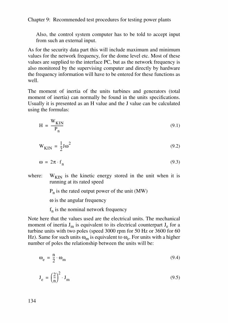
Chapter 9: Recommended test procedures for testing power plants
134
Also, the control system computer has to be told to accept inputfrom such an external input.
As for the security data part this will include maximum and minimumvalues for the network frequency, for the dome level etc. Most of thesevalues are supplied to the interface PC, but as the network frequency isalso monitored by the supervising computer and directly by hardwarethe frequency information will have to be entered for these functions aswell.
The moment of inertia of the units turbines and generators (totalmoment of inertia) can normally be found in the units specifications.Usually it is presented as an H value and the J value can be calculatedusing the formulas:
(9.1)
(9.2)
(9.3)
where: WKIN is the kinetic energy stored in the unit when it isrunning at its rated speed
Pn is the rated output power of the unit (MW)
ω is the angular frequency
fn is the nominal network frequency
Note here that the values used are the electrical units. The mechanicalmoment of inertia Jm is equivalent to its electrical counterpart Je for aturbine units with two poles (speed 3000 rpm for 50 Hz or 3600 for 60Hz). Same for such units ωm is equivalent to ωe. For units with a highernumber of poles the relationship between the units will be:
(9.4)
(9.5)
HWKIN
Pn---------------=
WKIN12---Jω2
=
ω 2π fn⋅=
ωen2--- ωm⋅=
Je2n---
2Jm⋅=

Recommended test procedures for testing power plants
135
where: n is the number of poles of the unit
As for information about the network that the unit may be workingonto in an emergency situation the following information is needed:
1. expected maximum step load change on the network
2. load level of the unit to be tested while in island operation
3. if other units are active on the simulated network one must have datafor their moment of inertia and, if they do take part in the frequencycontrol of the network, what model that should be used to simulatethem and what the time constants and droop values that theirsystems have.
9.4 Basic step response tests
A step response test similar to what is shown in Chapter 3 is not onlythe simplest test to perform but also the one that is the easiest to evalu-ate. If a slower rate of change of the load level of the simulated net-work is used then it becomes harder to determine time constants andharder to separate different effects from each other. Therefore e.g.ramp load changes would give less information.
As mentioned in Chapter 3 it is recommended with regard to securitythat the first tests are done with a fairly high value for the total momentof inertia present on the network (high J value). This gives a smootheroperation and large oscillations are far less likely. If such a test passesin a well behaved manner then one can easily repeat the test with lowerJ values. The lowest value that is meaningful to test is of course that ofthe unit under test. This is then equivalent to that this unit is the soleone supplying power to the island network and that no additionalmoment of inertia is present; e.g. large synchronous machines on theload side.
The size of the power step should for security reasons first be quitesmall. Then if the behaviour of the unit is stable and no problems areobserved one can test with larger steps. The maximum step size is setby what can be considered safe for the unit, with regard to thermal andmechanical stress. Steps of up to 10% of the rated power of the unitshould never present a problem in this respect, and for most types ofunits up to 20% would be safe as well.

Chapter 9: Recommended test procedures for testing power plants
136
For the basic step response tests it is always assumed that the unitunder test is the only one that performs any frequency control duties onthe network. Other units on the network are assumed to be operating inconstant power mode and their only presence in the simulation is thatthey contribute power (=reduce the load of the tested unit) and momentof inertia (increase the J value).
These tests are made with the simulator in its normal mode; i.e. with aclosed control loop where the simulator simulates the network andfeeds the frequency information back to the unit under test. This closedloop means that the test is made with a considerably higher level ofsecurity than if one would be using open loop test methods, whereerrors will have no way of correcting themselves.
9.5 Steam storage versus boiler response test
If one of the objectives of the test is to be able to build a control modelof the unit that is being tested then a test should be made to determinewhether or not there is a need for a boiler model for the unit in ques-tion. The determining factor here is whether or not the steam storagecapacity of the steam dome or the steam generators, or of the boileritself, depending on design, is large enough compared to the speed ofresponse of the boiler. If the steam storage capacity is large enough inthis respect the steam pressure at the point of delivery can for shortterm dynamics be assumed to be constant and there is then no need forcreating a boiler model.
This test should be done as follows: the unit is run at a power level sim-ilar to what would be the case if the unit is used for island operation.The measuring system must be connected so that the steam pressure atthe point of delivery from the boiler (dome pressure if the unit has asteam dome) is recorded. A step increase of the load in the simulatednetwork is then done. The step should be similar to the largest step loadchange that one can anticipate on the simulated island network. A valueof 10% of the current load should normally be sufficient. The higherload should be maintained for a period of time well beyond the timeconstant of the boiler system. If this is not known a time of 5 to 10 min-utes could be used.
Evaluating this test is quite simple. If the steam pressure at the end ofthe test is the same or slightly higher than what it was just before the

Recommended test procedures for testing power plants
137
step increase was applied, then there is no need for modelling theboiler. Obviously the firing control system and the boiler manage tokeep the pressure up also when the load increases.
If the pressure drops continuously during the test then the boiler sys-tem shows no response to the increased output power and the reasonfor this must be checked up. Either the system is in a manual controlmode and the operators failed to react or there is some technical mal-function, or some unit protection system has been activated. In the lat-ter case one will notice this easily, as the power output will also fail torespond to the load increase and the simulated network frequency willdrop rapidly.
Should however the steam pressure first drop in a significant mannerand then increase then the boiler response is obviously slower than thetime constant given by the steam storage and there may well be a needfor modelling the boiler and the fuel control system if a correct modelof the behaviour of the unit shall be made.
9.6 Parallel operation test
If one wants to test how the unit would behave in island operationworking parallel with other units that also take part in the frequencycontrol of the network, then these tests should be made in accordancewith the operating plans for such emergency operation. The other unitsshould be entered into the simulator with their models and their fre-quency control systems should be modelled with correct time constantsand droop values. Simple step load changes within the simulated net-work will then show the response of the different units. This result willbe only approximate for all but the tested unit, as the models used arequite crude ones, but as it is primarily the unit under test that we wantto have the operation characteristics of this will most of the time besufficient.
Note that this type of test will only give the response characteristics ofthe power stations with regard to their output power. This simulatorsystem, at least at its present state, does not take into account electro-mechanical oscillations between different units that could occur due totheir coupling through the network. The network is assumed to be stiffin this respect. Such oscillations are normally faster than the oscilla-tions that come from the frequency control process, the former having
Chapter 9: Recommended test procedures for testing power plants
138
typically a period of 1–2 s, the latter having 7–15 s or more. Networkoscillations due to the network coupling can be studied with commer-cial network simulation programs, such as Simpow or PSS/E.
9.7 Time constant test
The time constant of the high pressure turbine system and the dead-times of the same system and of the medium/low pressure systems, aswell as the control valve deadtime, are so short that the normal stepresponse tests will not give accurate information about them, as thesimulator cycle time is of the same order as these time constants. Usingthe same equipment one can however make a special test to determinethese with greater accuracy.
For this test the system is not running as a closed simulator controlloop but as an open circuit. A suitable value of the step signal to beapplied to the control input of the unit must first be determined basedon the basic step response tests mentioned above. This step of the out-put value is then applied to the unit for a few seconds. After this thesimulator returns to its normal operation.
As the simulator works in an open loop fashion during this test and alsodoes not need to communicate with the supervising computer, themeasurement speed can be increased considerably. Instead of onemeasurement per normal cycle in its normal mode (about 0.2 s) therecan be one measurement approximately every 20 ms, which is enoughin order to get a correct value of the short time constants of the system.
Note that since this test is made with an open loop, one has to be muchmore careful with the selection of the size of the disturbance; as thereis no selfcorrecting mechanism in action.
9.8 Power System Stabilizer test
If the unit to be tested is equipped with a Power System Stabilizer(PSS) then this one should be turned off during the initial tests. Thereason for this is that the PSS works through the voltage control systemand tries to stabilize the operation of the unit (minimize electrody-namic oscillations between this unit and other units on the network).

Recommended test procedures for testing power plants
139
This may mean that if there are oscillations of the output power duringthe tests, as is quite likely when the unit is tested for small values forthe moment of inertia, then there will be substantial changes in the out-put voltage. This is usually undesirable and often unacceptable.
Changes in the active power output of a unit that is synchronized onto alarge power system will have very small effects as far as the network isconcerned. The frequency is always the same in different parts of thenetwork, unless there are very large perturbations, something which atest of this type can not induce, and there is no need to worry aboutlocal effects on the network. With changes in the reactive power out-put, as the action of the PSS would lead to, it is quite different. Suchchanges translate immediately into local voltage variations and if thepower station is located in an area where the loads are sensitive to suchvariations then such operation will clearly not be allowed.
In addition, testing with the PSS active may not always give the infor-mation that we want primarily. As the PSS responds to a type of oscil-lations that we have not included in the simulator system, as thenetwork is not modelled in such a way that inter-machine oscillationscan be represented, the actions of the PSS will in most cases not be typ-ical for the way it would act in a real situation.
If one wants to test the behaviour of the PSS during a series of teststhen this should be done towards the end, when the approximate behav-iour of the unit with different load changes and J values is known rea-sonably well. A suitable combination of step size and J value shouldthen be chosen so that the resulting oscillations are quite small and thusthe actions of the PSS are limited. Before such a test one should makean assessment of how much voltage variations that can be tolerated inthe local area.
9.9 Tests on a planned network
If the power station is planned to be a part of a particular network setupfor emergency island operation then its behaviour in such a case can betested in a more direct way. The simulator system that was developedcontains load and network models that can be set to resemble theplanned network and thus give a more direct indication of how the unitto be tested can handle the situation.

Chapter 9: Recommended test procedures for testing power plants
140
If a test like this is to be made one needs more data; primarily a fulldescription of the network and a reasonable assumption as to the char-acteristics of the loads. After these have been entered the simulator per-forms a basic load-flow calculation, to get a start-up condition, andafter that the tests are done in the same manner as for the basic stepresponse tests described in Section 9.4. The difference is that we nowget a full network response, rather then just the response of one loadseemingly connected directly to the unit generator.
The network is described through a matrix representation. The programwill build an admittance matrix of the system, based on supplied datafor lines, transformers and shunts, add units of production and loadsand runs a load-flow calculation.
The load model used is a quite simple one, where the loads are dividedup into three parts: a constant load with no dependence on frequency(typical for e.g.electric heating), a load which is proportional to the fre-quency (typical for electric motors running against a constant torque)and a load which is proportional to the frequency to the power of three(typical for motors that run pumps and fans):
(9.6)
where: P = total load power
P0 = load that does not depend on frequency
P1 = load that is proportional to the frequency
P2 = load that is proportional to the frequency to the power ofthree
f = network frequency
fn = nominal network frequency
Tests run against the power station simulator indicate that the behav-iour of the power station with regard to frequency control characteris-tics are more critical when the load is constant, as compared to when itdepends on frequency. This is natural, as any dependence on the fre-quency means that the load is to some extent part of the frequency con-trol: when there is a shortage of power production the frequency willdrop and if the loads then drop as well it will relieve the situation, andvice versa if there is too large a production.
P P0 P1ffn-----⋅ P2
ffn-----
3⋅+ +=

Recommended test procedures for testing power plants
141
With the above in mind and also considering that it is generally hard toknow beforehand the load characteristics of the loads on a plannedemergency network, it may be safe to use only constant load for thesetests, unless one has clear figures showing that a major portion of theload to be handled in such a situation is highly frequency dependant, inwhich case this dependence should of course be modelled.
For a further description of the system used in the simulator to describethe network, see [2], where these systems are discussed in detail.
9.10 Load shedding tests
As the simulator has a load shedding model included in its networkdescription it is also possible to perform tests against a load sheddingsystem, to test under which circumstances that it will get activated andwhat influence it will have on the system and on the unit under test.
The setup is the same as for the tests described above and a load shed-ding test can either be done in combination with a basic step responsetest as described in Section 9.4 or as a part of a more complete networktest as described in Section 9.9.
To perform such a test the load is increased to beyond what the unit canrespond to. This can be in two ways: either as a direct step increase, inwhich case the problem will primarily not be that the unit can notdeliver the power needed but merely that it can often not do so fastenough, which will then trigger a load shedding, which will relieve thesystem situation, or the load can be gradually increased, pushing theunit towards what it is capable of responding to. The latter case cangenerally be thought of as less interesting, as the situation that we endup in that case is one where the outcome depends less on the automaticcontrol systems of the unit and more on the station operators and thenetwork dispatchers.
The load shedding system of the simulator consists of five steps of loadshedding. For each step two time limits and two activation frequenciesare set. The higher frequency limit will activate the step with a longertime delay, whereas a much shorter delay will be used if the lower limitis reached.

Chapter 9: Recommended test procedures for testing power plants
142
Corresponding to the load shedding there is a also an automatic loadreconnection system. If the network frequency has been restored tonormal for a set period of time the loads will gradually be reconnected.

Future work
143
Chapter 10 Future work
There is a potential to develop this test method still further and to beable to build more correct models of different power station units usingthis method.
Accuracy can be increased by the use of faster computer systems andfaster methods for the interchange of information between the differentparts of the simulator system. In addition the simulator system can bedeveloped into a commercial testing tool by developing a version thatis easily portable, based on a lap top computer system, and that canthus easily be brought to any unit that one wants to test.
The power station interface unit can also be improved, making it muchmore portable and making it able to connect to a broader range of tur-bine control systems.
Improvements can also be made to the security systems. These systemsare today developed far enough so that the risks of damage to the unitunder test can be said to be eliminated, but by improving these systemso that they can use computer prediction methods to determine whatwill happen next in the simulation process the risk of tripping the unitcan be still further reduced.
In addition to the hardware and security routine improvements men-tioned above there are also many possibilities for further improvementsto the software. Including any kind of inter-machine oscillations in thespecifications was considered to be impossible when this project wasstarted. It may still be, but with the extremely fast development of com-puters it should soon be possible to achieve enough processing capac-ity so that this kind of a simulator can also be built.
The software should also be structured and documented so that it canbe part of a commercial class software package. At the moment it isdocumented only in preliminary form; a documentation that is kept atthe Department of Electric Power Engineering at Chalmers.
As for the tests done within this project many more such tests shouldbe made with different types of power stations in order to be able tobuild models for different designs of power plant units. In order to beable to make long term models it is also necessary that such tests canbe made over longer period of time. During this project the availabilityof the power station for testing has been quite limited and such testscould therefore not be made.

Chapter 10: Future work
144

Conclusions
145
Chapter 11 Conclusions
The simulator testing method that has been developed in this project,where a simulator system is connected to the frequency control systemof the unit to be tested while the unit itself remains synchronized ontothe main network, is well suited for a variety of tests of a power stationunit. It is a simple and reliable way of testing the behaviour of the fre-quency control system and of other vital parts of the unit in particularwhen it comes to determining how the unit would respond if it wasused for island operation on a very limited network. The method hasthe potential to be developed into a standard test method for tests ofthis nature.
Tests made in this project show that thermal power plants with valvecontrol mode and with sufficient steam storage capacity are well suitedto be used for frequency control purposes. They have a very fastresponse to network load changes and with proper settings there shouldbe no major problems in using them in this fashion.
The widespread idea that thermal power plants are far less suited forfrequency control purposes as compared to hydro-electric units whichis well rooted in Sweden, as Sweden has always had a situation wherehydro power has been available in sufficient amounts to take care of allfrequency control duties, may not always be true. While hydro-electricunits are sturdy and reliable their speed can in most cases not comparewith thermal units of the types tested in this project.
In island operation it is essential to consider the moment of inertia onthe network, as well as the droop values of the frequency control sys-tems of the units responsible for the frequency control of the network.Both dispatch plans and controller settings may need to be modifiedcompared to what is used in normal operation on the main intercon-nected network.
Simple models can be built in order to model the dynamic behaviour ofthis cathegory of thermal power plants. For many purposes such mod-els may be fully sufficient.

Chapter 11: Conclusions
146

147
References
[1] Denegri G.B., Marconato R., Morini A., Pinceti P., Scarpellini P:,“Influence of the Auxiliary Systems Behaviour on Thermal Power PlantsResponse Following Large Perturbations”, IERE Workshop on “Newissues in Power System Simulation”, Caen, France, March 30-31, 1992.
[2] Andersson J., “Development of a Method of Analyzing the ControlCharacteristics of Thermal Power Plants and their Interaction with PowerSystems”, Technical report No. 161 L, Department of Electrical PowerSystems, Chalmers University of Technology, Gothenburg, Sweden, 1993,ISBN 91-7032-901-X
[3] Cheres E., “Small and Medium Size Drum Boiler Models Suitable forLong Term Dynamic Response”, IEEE Transactions on EnergyConversion, Vol.5, No.4, December1990.
[4] Andersson J., Stenborg B., “Simulator Methods for the Testing of theFrequency Control Behavior of Power Plants”, MEPS Modern ElectricPower Systems conference, Wroclaw, Poland, Sept.25-27, 1996.
[5] Jonsson S., Olefjord S., “Modellering av värmekraftverk”, Diploma ThesisNo.91/92:04, Department of Electrical Power Systems, ChalmersUniversity of Technology, Gothenburg, Sweden, 1991 (in Swedish).
[6] “Kartläggning av kraftstationernas effektresponsegenskaper vid snabbfrekvensändring i det synkrona Nordelnätet”, NOSY-report 3/1988 (inSwedish).
[7] Karsten Munkholm Larsen, “Momentan effektreserve i et ødriftsystem”,Lyngby, Denmark, July 1991 (in Danish).

148

149
Appendix A Specific results for the Stenungsund power station
The Stenungsund power station was used as a test object for thisproject for several reasons. One is that it was suitably located, beingone of the few conventional thermal power stations in Sweden. It isalso, with the exception of the turbines, of a quite conventional andinternationally very common design with an oil fired boiler, threesuperheaters, a high pressure turbine, a reheater, plus medium- and lowpressure turbines.
Apart from these general reasons for the choice of the Stenungsundpower station as the test object there was another important reason aswell: the station is located in a strategic position in case of emergencyoperation of the Swedish national network and it is therefore of primeinterest the study as whether e.g. island operation on a local network ispossible or not.
The results presented in this appendix are therefore results that areworth considering e.g. when making operating and discharge plans forthe local area around the Stenungsund power station.
Island operation using the Stenungsund power station,background
The Stenungsund power station is located in a strategic position, rea-sonably near Gothenburg, the second biggest city in Sweden. With its800 MW of total power it is by far not only the largest conventionalthermal power station of the region but also the largest station of anytype with exception of the nuclear power station at Ringhals, south ofGothenburg. The latter has four reactors with a combined output ofabout 3000 MW, but for security reasons it is unlikely that this or anynuclear generating station can be used in emergency situations.
The Stenungsund station is also built to be very well protected also inthe case of war or similar, as it is completely enclosed inside a moun-tain.
150
Another special circumstance that makes the Stenungsund stationinteresting as far as emergency planning goes is the fact that it is con-nected to the regional 130 kV network rather then to the Swedishnational transmission grid (400 kV), as is the case with e.g. the Ring-hals units. This means that if there is an emergency situation such thatthe 400 kV system is not available then the Stenungsund station willstill be able to deliver power, and it will then be the only station of itssize in the region. Power can in such a situation not be transferred fromother regions e.g. from hydroelectric units in the north of Sweden orfrom Norway, as without the 400 kV system the required transmissioncapacity is not available.
Situations where the 400 kV system is unavailable for a fairly longperiod of time can well be anticipated. Such situations could arise frommajor line faults, e.g. following hurricanes or other natural disasters,major transformer faults for main 400/130 kV transformers etc., plus ofcourse several situations that could arise in the case of war or sabotage.
In such a situation the Stenungsund power station would most likely bethe only large power station that would be able to supply power towestern Sweden. Other stations that would be likely to count on wouldbe the hydroelectric units at Olidan (130 MW) and Hajom (150 MW),plus a few smaller units. A special problem arises from the fact that theStenungsund station depends on external supplies for start-up as it hasno local emergency generator large enough to handle this. Thereforepower has to be transferred from either Olidan or Hajom. A direct 130kV line runs between these location so this start operation should notbe a major problem. However, if a local start power generator was to beadded to the Stenungsund plant it would add to its emergency capacityin this respect.
Moment of inertia
The Stenungsund units are, as mentioned earlier in this report, “light”units, i.e. they have unusually low H values. This is especially the casewith units 1 & 2, whose H value of 2.2 is extremely low. This is a cleardrawback in island operation and as the tests discussed in chapter 3clearly shows these units are likely to show a very unstable and oscil-lating behaviour if such a unit is left as the only machine on line in anisland system. A typical such oscillating behaviour is shown in the testseries below, which shows a series of step load changes applied to unit

151
1, in a situation corresponding to this one being the only unit on line.One should note here that these oscillations behaviour comes in spiteof the fact that the power level is low. A higher load level will generallycause the situation to deteriorate, as the ratio between the power pro-duced and the kinetic energy stored in the rotating machine is reduced.The kinetic energy depends only on the moment of inertia and thespeed of the unit and neither of these will increase with the powerlevel.
Figure A.1 Stenungsund, unit 1; power oscillations following a loadreduction.
If all four units at Stenungsund are in operation and there is most likelysome contributions to the moment of inertia from the participatinghydro power stations as well, then the combined moment of inertia getshigh enough so that the stability of the operation should not be a prob-lem.
As pointed out earlier it may be advantageous to use a higher numberof units than may be required by the load level simply to keep themoment of inertia up. For a load of 200 MW two units running at 100MW each are likely to give more stability than one unit at 200 MW,assuming that units 3 and 4 are used.
generator power
simulated frequency
152
Frequency control strategy
There are different frequency control strategies that can be used in asituation where Stenungsund and e.g. the units at Trollhättan (Olidanand Hajom) are to supply a local island network. Due to its speed ofresponse it may well be advantageous to use the Stenungsund units forfrequency control also when the hydro units are available. A schemewhere the hydro units operate with a lower droop but a slower responseand a thermal unit with higher droop but faster response may wellprove to provide the best frequency regulation.
However, it may not be recommended that all four units at Stenung-sund participate in the frequency control. There are two reasons forthis: one is that unless one has specifically tested such operation withtwo or more units in parallel one can not be certain that oscillationsbetween the two units will occur when there are sudden load levelchanges. The other reason is that a unit should not be run at or nearmaximum load in order to be suitable for frequency control. But in anisland operation situation all power that can possibly be delivered maywell be needed. In such a case the maximum yield will result from adispatch situation where three of the units are run at constant power,with the frequency control system deadband active, most likely fullrated power, and one unit at a lower level so that it will exhibit optimalfrequency control behaviour.
Special operating recommendations
Certain adjustments and changes may be required in an islanding situa-tion. One such adjustment could be to increase the droop value in orderto get a more stable operation and a better load distribution versus thehydro units, at the expense of course of the frequency accuracy.
Also the fuel/electric output differential protection system should prob-ably be set to signal only to prevent this system from incorrectly trip-ping the unit when there are large perturbations of the system;something which is far more likely on a small system.
Furthermore, several simulations have shown that keeping a good mar-gin with regard to the dome pressure is essential for stable operation.Normally one does not want to keep the dome pressure much higherthan required, as this translates into a lower overall efficiency andhence less economic operation. However, stability of operation must in

153
an emergency situation be given priority over efficiency and hence theunit should be operated with a somewhat higher dome pressure thanwhat would otherwise be used for the power level at which the unit isoperating. It seems preferable to keep the control valve opening in therange of 40 to 60%, as in this range the units have a quite sturdy andstable operation, provided that the moment of inertia of the system issufficiently high to aid in the damping of oscillations that may occur.
The feedwater system
The feedwater system appears to be the most critical system withregard to oscillations and island operation. At least this is the case forunits 3 and 4; for units 1 & 2 it is not possible to come to any conclu-sions regarding the behaviour of the feedwater system from the verylimited tests made on these units.
As pointed out in Chapter 7 the feedwater control system has timedelays that have a very unfortunate relationship to the time constant ofthe unit and power system oscillations as they occur if the unit is on itsown on the system. This means a highly increased risk of tripping theunit if oscillations occur.
The feedwater system time delays are for the most part built into thesystem; i.e. they consist of system time constants that can not bealtered without a major rebuilding of the system. Modifications madeto the control system itself may offer some improvements but these cannot be expected to be very radical. The main object of any suchchanges would be to speed up the response of the feedwater system tochanges in the high pressure steam flow rate. If the system could haveits response time reduced to about 60% of its present value the problemwould most likely be solved. This is however beyond what can beexpected from simple adjustments to the feedwater controller.
In a situation where the unit is alone on an island system and there is aproblem with oscillations then it may be well worth considering run-ning the feedwater system on manual control only. This will of courserequire the constant attention of the operators, but at least it will pre-vent the system from coming into counterphase with the steam flow inits attempts to follow the oscillating steam flow rate. If several units areon the network the moment of inertia is sufficient to slow the oscilla-tions down enough so that the feedwater system can follow the power /steam rate oscillations correctly.

154

155
Appendix B Measurement system, detailed description
Figure B.1 Measuring system, block diagram.
isolationamplifiers
16 channelmultiplexer A/D converter
computer
hard disk
source selectswitches
current tovoltageconverters
voltagedividers
current loopinputs
DC voltageinputs
AC voltage(potentiometer)inputs
rectifiers
RC filters
interfaceLANSupervisingcomputer
universalcounter
digitalmultimeter
transformer
from generatorbus CT
IEE
E-4
88 b
us

156
The measurement system consists of a PC A/D system with certain sig-nal processing systems. It is adapted so that it can be fitted to all signallevels that are commonly in use in power stations, e.g. 0 - 10 V DC, 0 -1 V DC, 0 - 20 mA, 0 - 50 mA,0 - 100 mA and 4 - 20 mA. All connec-tions are done via isolation amplifiers so that there will be no galvanicconnections and no ground loops between the measurement systemand the systems of the power station. The system also allows for digitalinput signals, e.g. to monitor alarm signals and similar. The same sys-tem also has digital output ports as well as D/A converters that are usedto generate signals that are fed to the power station and to the opera-tors, but these are discussed in Appendix C.
The A/D converters
There are 16 analog input channels that are A/D converted on a BostonTechnology PC30 general purpose measurement card. The card isinserted directly into the ISA bus of the PC that controls the power sta-tion interface.
The A/D converters are 12 bit converters, which gives a resolution ofapproximately + - 0.25%. Their input range can be set either to 0 - 10 VDC or to -10 - +10 V DC. The second range was normally used, exceptwhere a second A/D card was used for some special tests. This secondcard was then set to 0 - 10 V.
The converters are capable of a sampling rate of up to 30 kHz, butwhen the system is used as a simulator the measurement rate is limitedto one measurement per simulator cycle (i.e. every 0.2 s). Unfortu-nately this rate is limited by the data transfer rate between the differentcomputers making up the simulator.
Data from the A/D converters is fed to the computer over the bus as astream of 2 byte integers. This allows for a faster data transfer rate thenif floating point representation was to be used. It also highly reducesthe data storage requirements for the data. Very large datasets are gen-erated if longer tests are run, because of the many channels recorded.These values are stored in their integer form and conversion to floatingpoint will not be done until when the values are to be plotted during theevaluation at a later time.

157
The system is somewhat sensitive to the PC setup and the type of PCused. It was found that in certain cases the input channel multiplexercould come out of sequence with the controlling program. This is unac-ceptable as it means incorrect input to the simulation process. Fortu-nately this never happened on a sudden, random basis; instead certainPC combinations worked fine, others did not.
It should be noted that the original software drivers delivered with thePC30 card were extremely sensitive and too unreliable to be trusted foran application of this kind where 100% reliability is a necessity. Theversion tested was the FORTRAN language version, and when usingthese the system would sometimes just freeze or it would deliver com-pletely incorrect values. Much work was spent trying to solve theseproblems, but finally it was concluded that this driver package couldnot be used for this purpose if the simulator was to show a high degreeof reliability.
Instead of the original drivers a software package from Techsell, Stock-holm, was used. These drivers were considerably more reliable butunfortunately not available in Fortran. Instead all code running on thepower station interface computer had to be re-written in the C lan-guage. This was a quite large job, but the difference in reliability madeit worth it.
Measurement system front end inputs
All signals fed to the A/D converters have to be properly conditionedfirst. This is necessary in order to adapt the system to the transducers ofthe power station and in order to minimize noise on the signals and alsoin order to ascertain that all critical parts of the system have sufficientimmunity to the high level of electrical interference present in a powerstation.
In order to allow for using the simulator on different units and at differ-ent power stations it was also necessary to design the system so that avariety of input signals could be used. Acceptable input includes cur-rent loops of different values and DC signals at different levels. Forcertain signals, such as the generator voltage, the network frequencyand positions for valves and limiters AC signals can also be used.
158
All signals are fed via isolation amplifiers. This ascertains that therewill be no ground loops between the simulator and the control systemsof the power station. For most channels an integrated isolation ampli-fier chip, ISO 122 (Burr Brown). This amplifier provides an excellentlinearity (non-linearity less than 0.008% FSR), high speed (bandwidth50 kHz) and a high isolation voltage (1500 V) so that the integrity ofthe system will be guaranteed even in the event of large transients,“spikes” or similar on the input lines. A total of 12 such amplifierswere built. Each channel has its own dual power supply, which mini-mizes cross-talk and eliminates the risk of circuit to circuit flashovers.
The isolation amplifier has a normal input voltage range of -10 to +10V DC. Where lower levels were measured another amplifier was used,which had a 0 to 1 V DC input range.This input level was also used forrecording signals based on 0 to 20 mA, 0 to 50 mA or 0 to 100 mA cur-rent loops, using 50,20 and 10 ohms series resistors.
Most modern power station transducers or signal converters use aninterface based on a 4 to 20 mA current loop. For these a converterbased on the RCV 420 KP (Burr-Brown) IC. This chip has a very highaccuracy, with a non-linearity of 0.0002% (typical value) and also avery fast response (1.5 V/µS, typ.). Each of the ISO 122-based isola-tion amplifiers was fitted with such a converter so that the input rangecan be chosen as either -10 to + 10 V DC or 4 to 20 mA.
The transducers that translate the position of the control valve, the con-trol valve limiter and the intercept valve at the Stenungsund power sta-tion are based on potentiometer circuits that give an AC signal of up toapproximately 25 V. These signals were rectified using a diode bridgeand then attenuated to a 0 to 10 V DC range. An RC filter circuit with atime constant of about 0.1 s was added to produce a smooth DC signal.The signals were then fed to isolation amplifiers before being sent tothe A/D converters.
Frequency measurements
A precise and accurate way of measuring the network frequency isessential to the system. These frequency measurements are not as suchused during the simulation but monitoring the network frequency isvital to the operation of the security systems. The main reason for ter-minating a simulation prematurely is that the network frequency devi-

159
ates from its normal value. This would then indicate either a load losscondition or that there is a major disturbance on the power network. Ineither case the simulation has to be terminated and the unit switchedover to normal operation immediately. Failure to do so could in thecase of load loss lead to turbine overspeed and in the case of a networkdisturbance to that the disturbance is aggravated.
The prime frequency measurements are made using a Hewlett-PackardHP 5328A universal counter, which is connected via an IEEE-488measurement bus to the supervising computer. The data is then trans-ferred via the file I/O communication to the interface computer whereit is logged to the data file.Input to the universal counter is taken fromthe generator voltage: the output from one of the generator bus CTs isfed to a transformer that will reduce it to appr. 4 V AC which is thenfed to the counter.
A backup frequency measurement channel is set up by measuring thenormal output of the frequency sensing parts of the frequency controlsystem. This signal is, via an isolation amplifier, fed to an A/D con-verter and measured just like any process parameter. The decision as towhether it is out of bounds or not is made by the interface computer, sothat this vital checkup will function even if there should be a communi-cations problem between the interface computer and the supervisingcomputer. In the event of a problem with the interface computer thesupervising computer will in any case terminate the simulation; using aspecial relay link set up for this purpose.
The universal counter is operated in time period mode and measuresthe average period time of ten periods of the AC voltage. Thus a meas-urement is obtained at an interval of approximate 0.2 s and a highdegree of accuracy is achieved.
Generator voltage measurements
The generator voltage is continuously measured by a Hewlett-PackardHP 34401A multimeter, connected to one of the generator bus CTs anddelivering its output via an IEEE-488 interface to the supervising com-puter, for transfer to the interface computer and recording onto the logfile there. Measurements are made at a rate of one per second.

160

161
Appendix C The power station interface
The interface to the actual power station was considerably more com-plicated than the interface to the power station simulator. It consists ofseveral different units, even though they were all built into one box.
The station interface is controlled by a PC that is dedicated to this pur-pose. The actual interface to the computer is via a Boston TechnologyPC-30 multipurpose measurement and control card. The card isinserted into the PC and communicates with it via the PC bus.
The PC-30 card has 16 channels for A/D input, 2 channels for D/A out-put of 12 bits each, 2 channels for D/A of 8 bits each, three 16 bitcounters that can be set under program control and three digital I/Oports of 8 bits each.
The A/D channels are used for the measurement system as described inAppendix B.
In order for the simulations to be possible it was of course necessary todevelop a way of feeding a false control signal to the frequency controlsystem of the power station, and in the case of a voltage simulation alsoa voltage signal.
The frequency control system of units 3 and 4 at the Stenungsundpower station consists of a tachometer generator on the turbine axisand various control circuits. A simplified block diagram is shown inFigure C.1.
The first approach for supplying a simulated signal to the system wasto build a computer controlled power signal generator, able to generatea 400 Hz sine signal at 110 V level just like the tachometer generator.The frequency could then be accurately controlled by the computer andit was thought that this would be a true representation of the tachome-ter signal.A further description of the signal generator is found in [2].
The above approach failed. Several tests showed that the output signalfrom the discriminator circuit was very different when it was fed fromthe simulator and its signal generator as opposed to its normal opera-tion when the signal comes from the tachometer generator. The reasonfor this was that whereas the frequency of the tachometer generator
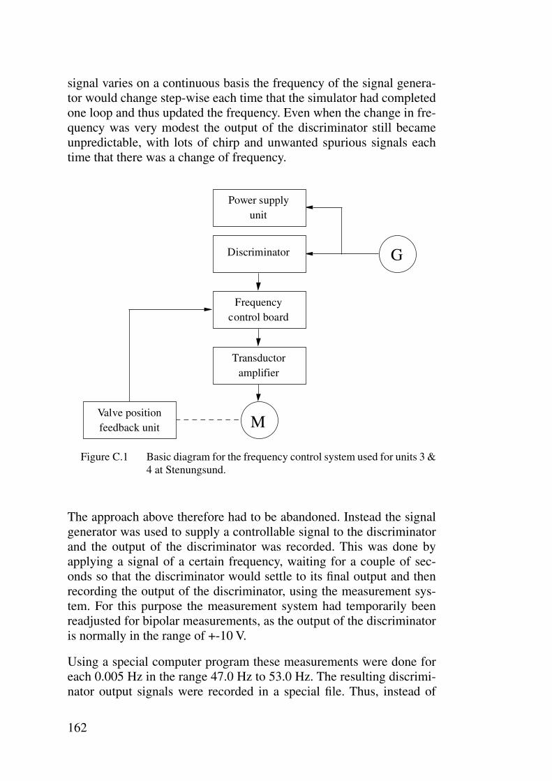
162
signal varies on a continuous basis the frequency of the signal genera-tor would change step-wise each time that the simulator had completedone loop and thus updated the frequency. Even when the change in fre-quency was very modest the output of the discriminator still becameunpredictable, with lots of chirp and unwanted spurious signals eachtime that there was a change of frequency.
Figure C.1 Basic diagram for the frequency control system used for units 3 &4 at Stenungsund.
The approach above therefore had to be abandoned. Instead the signalgenerator was used to supply a controllable signal to the discriminatorand the output of the discriminator was recorded. This was done byapplying a signal of a certain frequency, waiting for a couple of sec-onds so that the discriminator would settle to its final output and thenrecording the output of the discriminator, using the measurement sys-tem. For this purpose the measurement system had temporarily beenreadjusted for bipolar measurements, as the output of the discriminatoris normally in the range of +-10 V.
Using a special computer program these measurements were done foreach 0.005 Hz in the range 47.0 Hz to 53.0 Hz. The resulting discrimi-nator output signals were recorded in a special file. Thus, instead of
Power supplyunit
Discriminator G
Frequencycontrol board
Transductoramplifier
Valve positionfeedback unit M
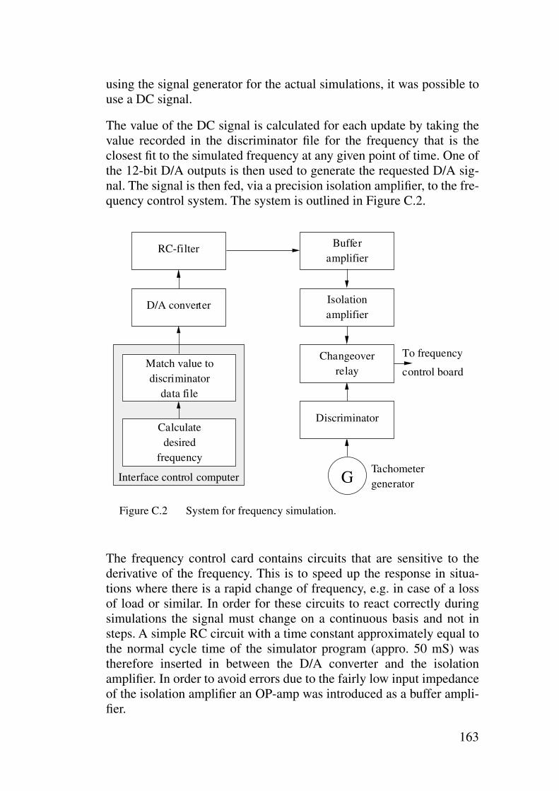
163
using the signal generator for the actual simulations, it was possible touse a DC signal.
The value of the DC signal is calculated for each update by taking thevalue recorded in the discriminator file for the frequency that is theclosest fit to the simulated frequency at any given point of time. One ofthe 12-bit D/A outputs is then used to generate the requested D/A sig-nal. The signal is then fed, via a precision isolation amplifier, to the fre-quency control system. The system is outlined in Figure C.2.
Figure C.2 System for frequency simulation.
The frequency control card contains circuits that are sensitive to thederivative of the frequency. This is to speed up the response in situa-tions where there is a rapid change of frequency, e.g. in case of a lossof load or similar. In order for these circuits to react correctly duringsimulations the signal must change on a continuous basis and not insteps. A simple RC circuit with a time constant approximately equal tothe normal cycle time of the simulator program (appro. 50 mS) wastherefore inserted in between the D/A converter and the isolationamplifier. In order to avoid errors due to the fairly low input impedanceof the isolation amplifier an OP-amp was introduced as a buffer ampli-fier.
Bufferamplifier
Discriminator
Isolationamplifier
Changeoverrelay
RC-filter
G
D/A converter
Calculatedesired
frequency
Match value todiscriminator
data file
Interface control computer
To frequency
control board
Tachometergenerator
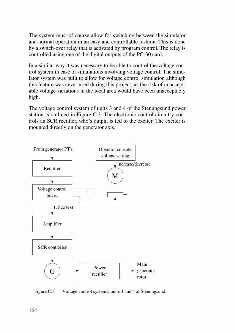
164
The system must of course allow for switching between the simulatorand normal operation in an easy and controllable fashion. This is doneby a switch-over relay that is activated by program control. The relay iscontrolled using one of the digital outputs of the PC-30 card.
In a similar way it was necessary to be able to control the voltage con-trol system in case of simulations involving voltage control. The simu-lator system was built to allow for voltage control simulation althoughthis feature was never used during this project, as the risk of unaccept-able voltage variations in the local area would have been unacceptablyhigh.
The voltage control system of units 3 and 4 of the Stenungsund powerstation is outlined in Figure C.3. The electronic control circuitry con-trols an SCR rectifier, who’s output is fed to the exciter. The exciter ismounted directly on the generator axis.
Figure C.3 Voltage control systems, units 3 and 4 at Stenungsund.
Rectifier
Voltage controlboard
M
Amplifier
SCR controller
PowerrectifierG
From generator PT's
Maingeneratorrotor
Operator consolevoltage setting
increase/decrease
1. See text

165
One approach would have been to simply take over the control signalfrom the voltage control system (point 1 in Figure C.3) and to supplythat from the interface via a D/A converter. This approach was howeverconsidered too risky, as if for some reason the simulator did notrespond correctly to any changes in voltage then the voltage wouldbecome uncontrollable and hazardous situations could occur in twoways: one could be the generation of overvoltages, even though theprotection systems would of course disconnect the generator in case ofexcessive voltages; another and more likely risk would be that the gen-erator would under such circumstances influence the voltage to the sur-rounding actual power network in such a way that it could creteproblems for power consumers. This would be particularly undesirableat Stenungsund, as several petro-chemical industries in the area arevery sensitive to voltage variations.
Instead it was decided that the correct way of controlling the voltagewas to control the actual request value, normally set by the voltagepotentiometer, and then let the normal control system handle the volt-age control in the normal fashion. In this case there would be no haz-ards involved if the computer system should get stuck or similar; thevoltage would just settle to its new value.
Just as for the frequency control system it was found proper to intro-duce an RC circuit so that the control inflicted on the system would becontinuous rather then step-wise; even though there is no circuit in thevoltage control system that uses the voltage derivative in any way.
The voltage request signal is generated by one of the 8-bit D/A con-verters, as the 12-bit ones had already been assigned to the signal gen-erator and to the disciminator output simulator circuit. In order to allowfor a good resolution a fixed voltage of an adjustable value (adjustedmanually via a potentiometer) was added to the signal, so that theentire 8-bit range of the D/A converter could be used for controllingthe voltage within the limits that it could possibly vary within.
A changeover relay, controlled via one of the digital I/O lines of thePC-30 card, switches between simulator mode and normal operation.
The final design of the voltage control system of the simulator is shownin Figure C.4.
The interface unit also contains the circuitry that is required for drivingthe power station operator interface unit. This unit allows the operatorsto monitor the progress of the simulation and also to immediately ter-minate the simulation, should that become necessary.

166
Figure C.4 Voltage simulation circuit.
During the tests performed at the Stenungsund power station it wasfound that various kinds of interference or transients could sometimesenter the circuits. This could result in that certain measured valueswere completely in error and this in turn could lead to incorrect actionby the simulator.
In order to prevent these problems from presenting a risk for malfunc-tion certain precautions had to be taken. Some were implemented inhardware; e.g. by adding decoupling capacitors and RC or LC filters tocertain connections within the interface unit. Other measures wereincluded in the software; like automatic rejection of unreasonable val-ues and double or triple checks that e.g. a certain command has beenreceived before any action is taken on the same.
D/A converter
Isolationamplifier
RC-circuit
Power amplifier
M
To voltagecontrol board
Changeoverrelay
Motor potentiometer foroperator voltage control

161
Bibliography
Adibi M., Kafka R., ”Power System Restoration Issues”, IEEE Computer Applica-tions in Power, April 1991, pp. 19-24.
Bargiotas D., Birdwell J., ”Residential Air Conditioner Dynamic Model for Direct Load Control”, IEEE Transactions on Power Delivery, Vol. 3, No. 4, October 1988, pp. 2119-2126.
Chong C., Malhami P., ”Statistical Synthesis of Physically Based Load Models with Applications to Cold Load Pickup”, IEEE Transactions on Power Apparatus and Systems, Vol. PAS-103, No. 7, July 1984, pp. 1621-1628.
CIGRÉ Study Committee 38, Working Group 02 Task Force No. 2, ”Modelling and Simulation of Black Start and Restoration of Electric Power Systems”, Electra, No. 147, April 1993, pp. 21-42.
CIGRÉ Study Committee 38, Working Group 02 Task Force No. 2, ”Modelling and Simulation of Black Start and Restoration of an Electric Power System Results of a Questionnaire”, Electra, No. 131 pp. 154-168.
CIGRÉ Study Committee 38, Working Group 06 Task Force No. 4, ”A Survey of Expert Systems for Power System Restoration”, Electra No. 150, October 1993, pp. 87-105.
Delfino B., Invernizzi M., Morini A., ”Knowledge-Based Restoration Guidlines”, IEEE Computer Applications in Power, July 1992, pp. 54-59.
Fountas N., Hatziargyriou N., Orfanogiannis C., Tasoulis A., ”Interactive Long-Term Simulation for Power System Restoration Planning”, IEEE/PES, Baltimore, USA, January 1996.
IEEE Committee Report, Adibi M., Adamski G., Jenkins R., Gill P., ” Nuclear Plant Requirements During Power System Restoration”, IEEE Transactions on Power Systems, Vol. 10, No. 3, August 1995, pp. 1486-1491.
IEEE Committee Report, Adibi M., Alexander R., Avramovic B., ”Overvoltage Control During Restoration”, IEEE Transactions on Power Systems, Vol. 7, No. 4, November 1992, pp. 1464-1470, IEEE/PES 1992 Winter Meeting, New York, Jan-uary 26-30, 1992.
IEEE Committee Report, Adibi M., Borkoski J., Kafka R., ”Analytical Tool Requirements for Power System Restoration”, IEEE Transactions on Power Sys-tems, Vol. 9, No. 3, August 1994, pp. 1582-1591.

162
IEEE Committee Report, Adibi M., Fink L., Andrews C., Arsanjani F., Lanier M., Miller J., Volkmann T., Wrubel J., ”Special Considerations in Power System Resto-ration”, IEEE Transactions on Power Systems, Vol. 7, No. 4, November 1992, pp. 1419-1427.
IEEE Committee Report, Adibi M., Fink L., Giri J., Kirschen D., Shahidehpour S., Zaborszky J., ”New Approaches in Power System restoration”, IEEE Transactions on Power Systems, Vol. 7, No. 4, November 1992, pp. 1428-1434.
IEEE Committee Report, Adibi M., Kafka R., Milanicz D., ”Expert System Requirements for Power System Restoration”, IEEE Transactions on Power Sys-tems, Vol. 9, No. 3, August 1994, pp. 1592-1600.
IEEE Committee Report, Adibi M., Milanicz D., ”Protective System Issues During Restoration”, IEEE Transactions on Power Systems, Vol. 10, No. 3, August 1995, pp. 1492-1497.
IEEE Committee Report, Cooper M. et al., ”Bulk Power System Restoration Train-ing Techniques”, IEEE Transactions on Power Systems, Vol. 8, No. 1, February 1993, pp. 191-197.
IEEE Committee Report, Forrest D., Albrecht P., Allan R., Bhavaraju M., Billinton R., Landgren G., McCoy M., Reppen N., ”Proposed Terms for Reporting and Ana-lyzing Outages of Electrical Transmission and Distribution Facilities”, IEEE Transactions on Power Apparatus and Systems, Vol. PAS-104, No. 2, February 1985, pp. 337-348.
IEEE Committee Report, Johnson W., Prabhakara F., Torri J., Niessink T., Gates J., Stovall J., Whitmire C., Mills L., Rodrigue J., ”System Restoration - Deploying the Plan”, IEEE Transactions on Power Apparatus and Systems, Vol. PAS-101, No. 11 November 1982, pp. 4623-4271.
IEEE Committee Report, Nielsen K., Adibi M., Barrie D., Cooper M., Heussner K., Robertson M., Scheidt J., Scheurer D., ”System Operations Challenges”, IEEE Transactions on Power Systems, Vol. 3, No. 1, February 1988, pp. 118-126.
IEEE Committee Report, Wunderlich S., Adibi M., Fischl R., Nwankpa C., ”An Approach to Standing Phase Angle Reduction”, IEEE Transactions on Power Sys-tems, Vol. 9, No. 1, February 1994, pp. 470-478.
Ihara S., Schweppe F., ”Physically Based Modelling of Cold Load Pickup”, IEEE Transactions on Power Apparatus and Systems, Vol. PAS-100, No. 9, September 1981, pp. 4142-4150.
Kafka R., Penders D., Bouchey S., ”Role of Interactive and Control Computers in the Development of a System Restoration Plan”, IEEE Transactions on Power Apparatus and Systems, Vol. PAS-101, No. 1, January 1982, pp. 43-52.

163
Kirschen D., Volkmann T., ”Guiding a Power System Restoration with an Expert System”, IEEE Transactions on Power Systems, Vol. 6, No. 2, May 1991, pp. 558-566.
Knight U, ”A Note on Strategy of Restoration”, Electra No. 114, pp. 108-111.
Knight U., ”System Restoration Following a Major Disturbance”, Electra, No. 106, pp. 34-61.
Kojima Y., Warashina S., Kato M., Watanabe H., ”The Development of Power Sys-tem Restoration Method for a Bulk Power System by Applying Knowledge Engi-neering Techniques”, IEEE Transactions on Power Systems, Vol. 4, No. 3, August 1989, pp. 1228-1235.
Kojima Y., Warashina S., Nakamura S., Matsumoto K., ”Development of a Guid-ance Method for Power System Restoration”, IEEE Transactions on Power Sys-tems, Vol. 4, No. 3, August 1989, pp. 1219-1227.
Lang W., Anderson M., Fannin D., ”An Analytical Method for Quantifying the Electrical Space Heating Component of a Cold Load Pick Up”, IEEE Transaction on Power Apparatus and Systems, Vol. PAS-101, No. 4, April 1982, pp. 924-932.
Laurent J., Malhame R., ”A Physically-Based Computer Model of Aggregate Elec-tric Water Heating Loads”, IEEE Transactions on Power Systems, Vol. 9, No. 3, August 1994, pp. 1209-1217.
Lindstrom R., ”Simulation and Field Tests of the Black Start of a Large Coal-Fired Generating Station Utilizing Small Remote Hydro Generation”, IEEE Transactions on Power Systems, Vol. 5, No. 1, February 1990, pp. 162-168.
Liu C., Lee S., Venkata S., ”An Expert System Operational Aid for Restoration and Loss Reduction of Distribution Systems”, IEEE Transactions on Power Systems, Vol. 3, No. 2, May 1988, pp. 619-626.
Liu C., Liou K., Chu R., Holen A., ”Generation Capability Dispatch for Bulk Power System Restoration: A Knowledge-Based Approach”, IEEE Transaction on Power Systems, Vol. 8, No. 1, February 1993, pp. 316-325.
Maeland A., ”Operator Assistance Using Knowledge-Based Technology for Power System Restoration”, Third Symposium on Expert Systems Application to Power systems, April 1-5, 1991, Tokyo-Kobe, Japan.
Mariani E., Mastroianni F., Romano V., ”Field Experiences in Reenergization of Electrical Networks from Thermal and Hydro Units”, IEEE Transactions on Power Apparatus and Systems, Vol. PAS-103, No. 7, July 1984, pp. 1707-1713.

164
Matsumoto K., Sakaguchi T., Kafka R., Adibi M., ”Knowledge-Based Systems as Operational Aids in Power System Restoration”, Proceedings of the IEEE, Vol. 80, No. 5, May 1992, pp. 689-696.
McDonald J., Bruning A., Mahieu W., ”Cold Load Pickup”, IEEE Transactions on Power Apparatus and Systems, Vol. PAS-98, No. 4, July/August 1979, pp. 1384-1386.
Mondon E., Heilbronn B., Harmand Y., Paillet O., Fargier H., ”An Aid for Network Restoration After a Local Disturbance”, IEEE Transactions on Power Systems, Vol. 7, No. 2, May 1992, pp. 850-855.
Morelato A., Monticelli A., ”Heuristic Search Approch to Distribution System Res-toration”, IEEE Transactions on Power Delivery, Vol. 4, No. 4, October 1989, pp. 2235-2241.
Morin G., ”Service Restoration Following a Major Failure on the Hydro-Qubec Power System”, IEEE Transactions on Power Delivery, Vol. PWRD-2, No. 2, April 1987, pp. 454-462.
Mortensen R., Haggerty K., ”Dynamics of Heating and Cooling Loads: Models, Simulation, and Actual Utility Data”, IEEE Transactions on Power Systems, Vol. 5, No. 1, February 1990, pp. 243-249.
Nadira R., Dy Liacco T., Loparo K., ”A Hierarchical Interactive Approach to Elec-tric Power System Restoration”, IEEE Transactions on Power Systems, Vol. 7, No. 3, August 1992, pp. 1123-1131.
Nehrir M., Dolan P., Gerez V., Jameson W., ”Development and Validation of a Physically-Based Computer Model for Predicting Winter Electric Heating Loads”, IEEE Transaction on Power Systems, Vol. 10, No. 1 February 1995, pp. 266-272.
Oliver B., Rose D., ”Practices on Black Start of Power Stations”, Electra, No. 121, pp. 78-85.
Ross H., Zhu N., Giri J., Kindel B., ”An AGC Implementation for System Island-ing and Restoration Conditions”, IEEE Transactions on Power Systems, Vol. 9, No. 3 , August 1994, pp. 1399-1410.
Shah S., Shahidehpour S., ”A Heuristic Approach to Load Shedding Scheme”, IEEE Transactions on Power Systems, Vol. 4, No. 4, October 1989, pp. 1421-1429.
Shimakura K., Inagaki J., Matsunoki Y., Ito M., Fukui S., Hori S., ”A Knowledge-Based Method for Making Restoration Plan of Bulk Power System”, IEEE Trans-actions on Power Systems, Vol. 7, No. 2, May 1992, pp. 914-920.
165
Shimakura Y., Inagaki J., Fukui S., Hori S., ”Knowledge-Based Approach for the Determination of Restorative Operation Procedures for Bulk Power Systems”, Electrical Power & Energy Systems, Vol. 16, No. 3, 1994, pp. 183-190.
Shultz R., Mason G., ”Blackstart Utilization of Remote Combustion Turbines, Analytical Analysis and Field Test”, IEEE Transaction on Power Apparatus and Systems, Vol. PAS-103, No. 8, August 1984, pp. 2186-2191.
Smith J., Connor D., Bose A., Burton E., ”Development of Operator Training Cur-ricula Using the Instructional Systems Development Approach”, IEEE Transac-tions on Power Apparatus and Systems, Vol. PAS-104, No. 12, December 1985, pp. 3446-3452.
Walve K., ”Modelling of Power System Components at Severe Disturbances”, CIGRÉ Report 38-18, Paris, August 27-September 4, 1986.
Wu F., Monticelli A., ”Analytical Tools for Power System Restoration - Concep-tual Design”, IEEE Transactions on Power Systems, Vol. 3, No. 1, pp. 10-16.
Yolcu M., Zaber Z., Birenbaum L., Granek S., ”Adaption of the Simplex Algorithm to Modelling of Cold Load Pickup of a Large Secondary Network Distribution System”, IEEE Transactions on Power Apparatus and Systems, Vol. PAS-102, No. 7 , July 1983, pp. 2064-2068.

166