the analytic hierarchy process (ahp) for decision … the analytic hierarchy process (ahp) for...
TRANSCRIPT

1
The Analytic HierarchyProcess (AHP)
for Decision MakingBy Thomas Saaty
Decision Making involvessetting priorities and the AHPis the methodology for doingthat.
Real Life Problems Exhibit:
Strong Pressures and Weakened Resources
Complex Issues - Sometimes There are No “Right” Answers
Vested Interests
Conflicting Values

2
Most Decision Problems are Multicriteria
• Maximize profits• Satisfy customer demands• Maximize employee satisfaction• Satisfy shareholders• Minimize costs of production• Satisfy government regulations• Minimize taxes• Maximize bonuses
Decision Making
Decision making today is a science. People have hard decisions to make and they need help because many lives may be involved, the survival of the business depends on making the right decision, or because future success and diversification must survive competition and surprises presented by the future.

3
WHAT KIND AND WHAT AMOUNT OFKNOWLEDGE TO MAKE DECISIONS
Some people say
• What is the use of learning about decision making? Life is so complicated that the factors which go into a decision are beyond our ability to identify and use them effectively.
I say that is not true.
•We have had considerable experience in the past thirty years to structure and prioritize thousands of decisions in all walks of life. We no longer think that there is a mystery to making good decisions.
• Decision Making involves all kinds of tradeoffs among intangibles. To make careful tradeoffs we need to measure things because a bad may be much more intense than a good and the problem is not simply exchanging one for the other but they must be measured quantitatively and swapped.
• One of the major problems that we have had to solve has been how to evaluate a decision based on its benefits, costs, opportunities, and risks. We deal with each of these four merits separately and then combine them for the overall decision.
THE GOODS THE BADS AND THE INTANGIBLES

4
3 Kinds of Decisionsa) Instantaneous and personal like what restaurant to eat at and what kind of rice cereal to buy; b) Personal but allowing a little time like which job to choose and what house to buy or car to drive; c) Long term decisions and any decisions that involve planning and resource allocation and more significantly group decision making.
We can use the AHP and ANP as they are. Personal decisions need to be automated with data and judgments by different types of people so every individual can identify with one of these groups whose judgments for the criteria he would use and which uses the rating approach for all the possible alternatives in the world so one can quickly choose what he prefers after identifying with that type of people. A chip needs to be installed for this purpose for example in a cellular phone.
Knowledge is Not in the NumbersIsabel Garuti is an environmental researcher whose father-in-law is a master chef in Santiago, Chile. He owns a well known Italian restaurant called Valerio. He is recognized as the best cook in Santiago. Isabel had eaten a favorite dish risotto ai funghi, rice with mushrooms, many times and loved it so much that she wanted to learn to cook it herself for her husband, Valerio’s son, Claudio. So she armed herself with a pencil and paper, went to the restaurant and begged Valerio to spell out the details of the recipe in an easy way for her. He said it was very easy. When he revealed how much was needed for each ingredient, he said you use a little of this and a handful of that. When it is O.K. it is O.K. and it smells good. No matter how hard she tried to translate his comments to numbers, neither she nor he could do it. She could not replicate his dish. Valerio knew what he knew well. It was registered in his mind, this could not be written down and communicated to someone else. An unintelligent observer would claim that he did not know how to cook, because if he did, he should be able to communicate it to others. But he could and is one of the best.

5
Valerio can say, “Put more of this than of that, don’t stir so much,” and so on. That is how he cooks his meals - by following his instincts, not formalized logically and precisely. The question is: How does he synthesize what he knows?
Knowing Less, Understanding More
You don’t need to know everything to get to the answer.
Expert after expert missed the revolutionary significance of what Darwin had collected.Darwin, who knew less, somehow understood more.

6
An elderly couple looking for a town to which theymight retire found Summerland, in Santa BarbaraCounty, California, where a sign post read:
SummerlandPopulation 3001Feet Above Sea Level 208Year Established 1870
Total 5079
“Let’s settle here where there is a sense of humor,” saidthe wife; and they did.
Aren’t Numbers Numbers?We have the habit to crunch numbers
whatever they are
Do Numbers Have an Objective Meaning?Butter: 1, 2,…, 10 lbs.; 1,2,…, 100 tons
Sheep: 2 sheep (1 big, 1 little)
Temperature: 30 degrees Fahrenheit to New Yorker, Kenyan, Eskimo
Since we deal with Non-Unique Scales such as [lbs., kgs], [yds, meters], [Fahr., Celsius] and such scales cannot be combined, we needthe idea of PRIORITY.
PRIORITY becomes an abstract unit valid across all scales.
A priority scale based on preference is the AHP way to standardize non-unique scales in order to combine multiple criteria.

7
Nonmonotonic Relative Nature of Absolute Scales
Good forpreserving food
Bad for preserving food
Good for preserving food
Bad forcomfort
Good forcomfort
Bad forcomfort
100
0
Temperature
OBJECTIVITY!?
Bias in upbring: objectivity is agreed upon subjectivity. We interpret and shape the world in our own image. We pass it along as fact. In the end it is all obsoleted by the next generation.
Logic breaks down: Russell-Whitehead Principia; Gödel’s Undecidability Proof.
Intuition breaks down: circle around earth; milk and coffee.
How do we manage?

8
Making a Decision
Widget B is cheaper than Widget A
Widget A is better than Widget B
Which Widget would you choose?
Basic Decision Problem
Criteria: Low Cost > Operating Cost > Style
Car: A B BV V V
Alternatives: B A A
Suppose the criteria are preferred in the order shown and thecars are preferred as shown for each criterion. Which carshould be chosen? It is desirable to know the strengths of preferences for tradeoffs.

9
To understand the world we assume that:
We can describe it
We can define relations between its parts and
We can apply judgment to relate theparts according to
a goal or purpose that wehave in mind.
GOAL
CRITERIA
ALTERNATIVES
Hierarchic
Thinking
10
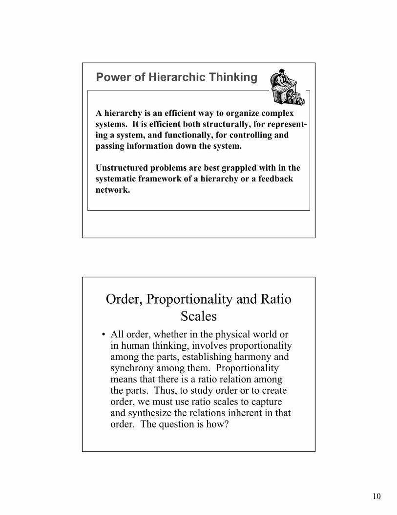
Power of Hierarchic Thinking
A hierarchy is an efficient way to organize complexsystems. It is efficient both structurally, for represent-ing a system, and functionally, for controlling and passing information down the system.
Unstructured problems are best grappled with in the systematic framework of a hierarchy or a feedbacknetwork.
Order, Proportionality and Ratio Scales
• All order, whether in the physical world or in human thinking, involves proportionality among the parts, establishing harmony and synchrony among them. Proportionality means that there is a ratio relation among the parts. Thus, to study order or to create order, we must use ratio scales to capture and synthesize the relations inherent in that order. The question is how?

11
Relative MeasurementThe Process of Prioritization
In relative measurement a preference, judgmentis expressed on each pair of elements with respect to a common property they share.
In practice this means that a pair of elementsin a level of the hierarchy are compared with respect to parent elements to which they relate in the level above.
If, for example, we are comparing two applesaccording to weight we ask:
• Which apple is bigger?
• How much bigger is the larger than the smaller apple?Use the smaller as the unit and estimate how many more times bigger is the larger one.
• The apples must be relatively close (homogeneous) if we hope to make an accurate estimate.
Relative Measurement (cont.)

12
•The Smaller apple then has the reciprocal value when compared with the larger one. There is no way to escape this sort of reciprocal comparison when developing judgments•If the elements being compared are not all homogeneous, they areplaced into homogeneous groups of gradually increasing relative sizes (homogeneous clusters of homogeneous elements). • Judgments are made on the elements in one group of small elements, and a “pivot” element is borrowed and placed in the next larger group and its elements are compared. This use of pivot elements enables one to successively merge the measurements of all the elements. Thus homogeneity serves to enhance the accuracy of measurement.
Relative Measurement (cont.)
Comparison MatrixGiven: Three apples of different sizes.
SizeComparison Apple A Apple B Apple C
Apple A S1/S1 S1/S2 S1/S3
Apple B S2 / S1 S2 / S2 S2 / S3
Apple C S3 / S1 S3 / S2 S3 / S3
Apple A Apple B Apple C
We Assess Their Relative Sizes By Forming Ratios

13
Pairwise ComparisonsSize
Apple A Apple B Apple C
SizeComparison
Apple A Apple B Apple C
Apple A 1 2 6 6/10 A
Apple B 1/2 1 3 3/10 B
Apple C 1/6 1/3 1 1/10 C
When the judgments are consistent, as they are here, any normalized column gives the priorities.
ResultingPriority Eigenvector
Relative Sizeof Apple
Pairwise Comparisons using Judgments and the Derived Priorities
Nicer ambience comparisons
Paris London New York
Normalized Total
0.5815
0.3090
0.1095
1
0.5328
0.1888
Paris
London
New York
1
1
1
2 5
31/2
1/5 1/3

14
Pairwise Comparisons using Judgments and the Derived Priorities
1
0.4297
0.1780
0.6220
0.2673
0.1107
1 3 7
1/3 1 5
1/7 1/5 1
TotalNormalized
B. Clinton M. Tatcher G. Bush
Politician comparisons
B. Clinton
M. Tatcher
G. Bush
In scoring one guesses at numbers to assign to things and when one normalizes, everything falls between zero and one and can look respectable because if we know the ordinal ranking of things, then assigning them comparable numbers yields decimals that have the appropriate order and also differ by a little from each other and lie between zero and one, it sounds fantastic despite guessing at the numbers.Paired comparisons is a scientific process in which the smaller or lesser element serves as the unit and the larger or greater one is estimated as a multiple of that unit. Although one can say that here too we have guessing but it is very different because we know what we are supposed to do and not just pull a number out of a hat. Therefore one would expect better answers from paired comparisons. If the person making the comparisons knows nothing about the elements being compared, his outcome would be just as poor as the other. But if he does know the elements well, one would expect very good results.
SCORING AND PAIRED COMPARISONS

15
When the judgments are consistent, we have two ways to get the answer:
1. By adding any column and dividing each entry by the total, that is by normalizing the column, any column gives the same result. A quick test of consistency if all the columns give the same answer.
2. By adding the rows and normalizing the result.
When the judgments are inconsistent we have two ways to get the answer:
1. An approximate way: By normalizing each column, forming the row sums and then normalizing the result.
2. The exact way: By raising the matrix to powers and normalizing its row sums
Consistency
In this example Apple B is 3 times larger than Apple C. We can obtain this value directly from the comparisons of Apple A with Apples B & C as 6/2 = 3. But if we were to use judgment we may have guessed it as 4. In that case we would have been inconsistent.
Now guessing it as 4 is not as bad as guessing it as 5 or more. The farther we are from the true value the more inconsistent we are. The AHP provides a theory for checking the inconsistency throughout the matrix and allowing a certain level of overall inconsistency but not more.

16
• Consistency itself is a necessary condition for a better understanding of relations in the world but it is not sufficient. For example we could judge all three of the apples to be the same size and we would be perfectly consistent, but very wrong.
• We also need to improve our validity by using redundantinformation.
• It is fortunate that the mind is not programmed to be alwaysconsistent. Otherwise, it could not integrate new informationby changing old relations.
Consistency (cont.)
Consistency (cont.)
Because the world of experience is vast and we deal with it in pieces according to whatever goals concern us at the time, our judgments can never be perfectly precise.
It may be impossible to make a consistent set of judgments on some pieces that make them fit exactly with another consistent set of judgments on other related pieces. So we may neither be able to be perfectly consistent nor want to be.
We must allow for a modicum of inconsistency. This explanation is the basis of fuzziness in knowledge. To capture this kind of fuzziness one needs ratio scales.
Fuzzy Sets have accurately identified the nature of inconsistency in measurement but has not made the link with ratio scales to make that measurement even more precise and grounded in a sound unified theory of ratio scales. Fuzzy Sets needs the AHP!

17
How Much Inconsistency to Tolerate?• Inconsistency arises from the need for redundancy. • Redundancy improves the validity of the information about the real world.• Inconsistency is important for modifying our consistent understanding, but it must not be too large
to make information seem chaotic.• Yet inconsistency cannot be negligible; otherwise, we would be like robots unable to change our
minds.• Mathematically the measurement of consistency should allow for inconsistency of no more than
one order of magnitude smaller than consistency. Thus, an inconsistency of no more than 10% can be tolerated.
• This would allow variations in the measurement of the elements being compared without destroying their identity.
• As a result the number of elements compared must be small, i.e. seven plus or minus two. Being homogeneous they would then each receive about ten to 15 percent of the total relative value in the vector of priorities.
• A small inconsistency would change that value by a small amount and their true relative value would still be sufficiently large to preserve that value.
• Note that if the number of elements in a comparison is large, for example 100, each would receive a 1% relative value and the small inconsistency of 1% in its measurement would change its value to 2% which is far from its true value of 1%.
Consistency (cont.)
Comparison of Intangibles
The same procedure as we use for size can be used to compare things with intangible properties. For example, we could also compare the apples for:
• TASTE• AROMA• RIPENESS

18
The Analytic Hierarchy Process (AHP)is the Method of Prioritization
• AHP captures priorities from paired comparison judgments of the• elements of the decision with respect to each of their parent criteria.
• Paired comparison judgments can be arranged in a matrix.
• Priorities are derived from the matrix as its principal eigenvector,• which defines a ratio scale. Thus, the eigenvector is an intrinsic • concept of a correct prioritization process. It also allows for the • measurement of inconsistency in judgment.
• Priorities derived this way satisfy the property of a ratio scale• just like pounds and yards do.
Decision MakingWe need to prioritize both tangible and intangible criteria:
♦ In most decisions, intangibles such as• political factors and• social factors
take precedence over tangibles such as• economic factors and• technical factors
♦ It is not the precision of measurement on a particular factorthat determines the validity of a decision, but the importancewe attach to the factors involved.
♦ How do we assign importance to all the factors and synthesizethis diverse information to make the best decision?

19
Verbal Expressions for Making Pairwise Comparison Judgments
Equal importance
Moderate importance of one over another
Strong or essential importance
Very strong or demonstrated importance
Extreme importance
1 Equal importance
3 Moderate importance of one over another
5 Strong or essential importance
7 Very strong or demonstrated importance
9 Extreme importance
2,4,6,8 Intermediate values
Use Reciprocals for Inverse Comparisons
Fundamental Scale of Absolute NumbersCorresponding to Verbal Comparisons
20
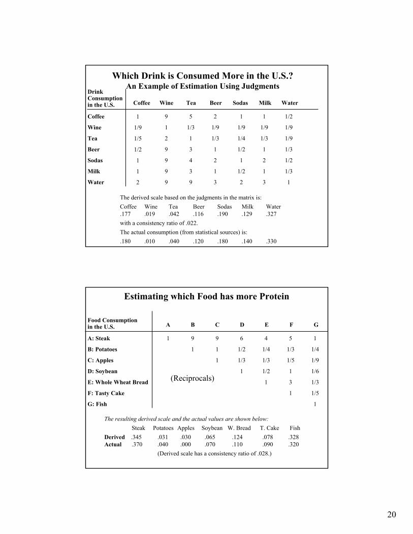
Which Drink is Consumed More in the U.S.?An Example of Estimation Using Judgments
Coffee Wine Tea Beer Sodas Milk Water
DrinkConsumptionin the U.S.
Coffee
Wine
Tea
Beer
Sodas
Milk
Water
1
1/9
1/5
1/2
1
1
2
9
1
2
9
9
9
9
5
1/3
1
3
4
3
9
2
1/9
1/3
1
2
1
3
1
1/9
1/4
1/2
1
1/2
2
1
1/9
1/3
1
2
1
3
1/2
1/9
1/9
1/3
1/2
1/3
1
The derived scale based on the judgments in the matrix is:Coffee Wine Tea Beer Sodas Milk Water.177 .019 .042 .116 .190 .129 .327with a consistency ratio of .022.The actual consumption (from statistical sources) is:.180 .010 .040 .120 .180 .140 .330
Estimating which Food has more Protein
A B C D E F GFood Consumptionin the U.S.
A: Steak
B: Potatoes
C: Apples
D: Soybean
E: Whole Wheat Bread
F: Tasty Cake
G: Fish
1 9
1
9
1
1
6
1/2
1/3
1
4
1/4
1/3
1/2
1
5
1/3
1/5
1
3
1
1
1/4
1/9
1/6
1/3
1/5
1
The resulting derived scale and the actual values are shown below:Steak Potatoes Apples Soybean W. Bread T. Cake Fish
Derived .345 .031 .030 .065 .124 .078 .328Actual .370 .040 .000 .070 .110 .090 .320
(Derived scale has a consistency ratio of .028.)
(Reciprocals)

21
Weight Radio Typewriter Large Attache
Case
Projector Small Attache
Eigenvector Actual Relative Weights
Radio 1 1/5 1/3 1/4 4 0.09 0.10Typewriter 5 1 2 2 8 0.40 0.39
Large Attache Case
3 1/2 1 1/2 4 0.18 0.20
Projector 4 1/2 2 1 7 0.29 0.27Small Attache Case
1/4 1/8 1/4 1/7 1 0.04 0.04
WEIGHT COMPARISONS
Comparison of Distances
from Philadelphia
Cairo Tokyo Chicago San Francisco
London Montreal Eigen-vector
Distance to Philadelphia in miles
Relative Distance
Cairo 1 1/2 8 3 3 7 0.263 5,729 0.278Tokyo 3 1 9 3 3 9 0.397 7,449 0.361Chicago 1/8 1/9 1 1/6 1/5 2 0.033 660 0.032San Francisco
1/3 1/3 6 1 1/3 6 0.116 2,732 0.132
London 1/3 1/3 5 3 1 6 0.164 3,658 0.177Montreal 1/7 1/9 1/2 1/6 1/6 1 0.027 400 0.019
DISTANCE COMPARISONS

22
F1
F2
F3
Fig.1 : L1 = 9 , H1 = 1P = 20
L1
H1
Fig.2: L2 = 8 , H2 = 2P = 20
Fig.3 : L3 = 7 , H3 = 3P = 20
L2
L3
H2
H3
F4Fig.4 : L4 = 6 , H4 = 4P = 20H4
L4
Perimeter Problem
2046F4
2037F3
2028F2
2019F1
PerimeterWidthLength
All Four Figures have the same Perimeter
.25
.25
.25
.25
Relative

23
Nagy Airline Market Share Model
Model Actual
(Yr 2000)
American 23.9 24.0
United 18.7 19.7
Delta 18.0 18.0
Northwest 11.4 12.4
Continental 9.3 10.0
US Airways 7.5 7.1
Southwest 5.9 6.4
Amer.West 4.4 2.9

24
14.613.01,032,000TESS
20.922.51,778,951BCP
64.564.55,104,000TELESP
7,914,051Total
RelativeShare(Model)
RelativeShare(Income)
Income

25
Comparación Modelo ANP v/s Realidad Actual.
ANP Results Actual Results
Asociación Chilena de Seguridad (ACHS) 52,0 % 52,6 %
Mutual de Seguridad 35,5 % 34,8 %
Instituto Seguros del Trabajo (IST) 12,5 % 12,6 %
Total 100,0 % 100,0 %
otas:
) El “Actual Results”, se obtiene a partir del número de trabajadores actualmente afiliados a las diferentes mutuales (privadas), que administran

26
Extending the 1-9 Scale to 1- ∞
•The 1-9 AHP scale does not limit us if we know how to use clustering of similar objects in each group and use the largest element in a group as the smallest one in the next one. It serves as a pivot to connect the two.
•We then compare the elements in each group on the 1-9 scale get the priorities, then divide by the weight of the pivot in that group and multiply by its weight from the previous group. We can then combine all the groups measurements as in the following example comparing a very small cherry tomato with a very large watermelon.
.07 .28 .65Cherry Tomato Small Green Tomato Lime
.08 .22 .70Lime
1=.08.08
.65 1=.65
Grapefruit
2.75=.08.22
.65 2.75=1.79
Honeydew
8.75=.08.70
.65 8.75=5.69
.10 .30 .60Honeydew
1=.10.10
5.69 1=5.69
Sugar Baby Watermelon
3=.10.30
5.69 3=17.07
Oblong Watermelon
6=.10.60
5.69 6=34.14This means that 34.14/.07 = 487.7 cherry tomatoes are equal to the oblong watermelon

27
53
Clustering & ComparisonColor
How intensely more green is X than Y relative to its size?
Honeydew Unripe Grapefruit Unripe Cherry Tomato
Unripe Cherry Tomato Oblong Watermelon Small Green Tomato
Small Green Tomato Sugar Baby Watermelon Large Lime
GoalSatisfaction with School
Learning Friends School Vocational College MusicLife Training Prep. Classes
SchoolA
SchoolC
SchoolB

28
School Selection
L F SL VT CP MCLearning 1 4 3 1 3 4 .32
Friends 1/4 1 7 3 1/5 1 .14
School Life 1/3 1/7 1 1/5 1/5 1/6 .03
Vocational Trng. 1 1/3 5 1 1 1/3 .13
College Prep. 1/3 5 5 1 1 3 .24
Music Classes 1/4 1 6 3 1/3 1 .14
Weights
Comparison of Schools with Respectto the Six Characteristics
LearningA B C
Priorities
A 1 1/3 1/2 .16
B 3 1 3 .59
C 2 1/3 1 .25
FriendsA B C
Priorities
A 1 1 1 .33
B 1 1 1 .33
C 1 1 1 .33
School LifeA B C
Priorities
A 1 5 1 .45
B 1/5 1 1/5 .09
C 1 5 1 .46
Vocational Trng.A B C
Priorities
A 1 9 7 .77
B 1/9 1 1/5 .05
C 1/7 5 1 .17
College Prep.A B C
Priorities
A 1 1/2 1 .25
B 2 1 2 .50
C 1 1/2 1 .25
Music ClassesA B C
Priorities
A 1 6 4 .69
B 1/6 1 1/3 .09
C 1/4 3 1 .22
29
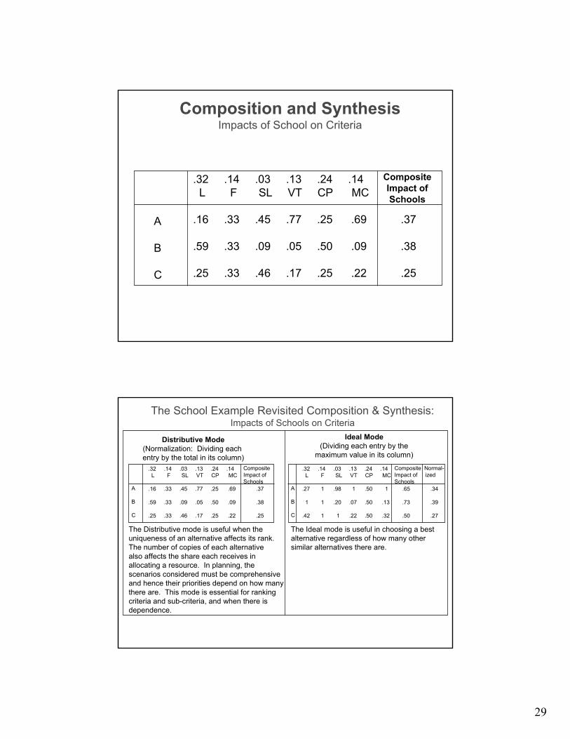
Composition and SynthesisImpacts of School on Criteria
CompositeImpact ofSchools
A
B
C
.32 .14 .03 .13 .24 .14L F SL VT CP MC
.16 .33 .45 .77 .25 .69 .37
.59 .33 .09 .05 .50 .09 .38
.25 .33 .46 .17 .25 .22 .25
The School Example Revisited Composition & Synthesis:Impacts of Schools on Criteria
Distributive Mode(Normalization: Dividing each entry by the total in its column)
A
B
C
.32 .14 .03 .13 .24 .14L F SL VT CP MC
.16 .33 .45 .77 .25 .69 .37
.59 .33 .09 .05 .50 .09 .38
.25 .33 .46 .17 .25 .22 .25
CompositeImpact ofSchools
A
B
C
.32 .14 .03 .13 .24 .14L F SL VT CP MC
.27 1 .98 1 .50 1 .65 .34
1 1 .20 .07 .50 .13 .73 .39
.42 1 1 .22 .50 .32 .50 .27
Composite Normal-Impact of izedSchools
Ideal Mode(Dividing each entry by the
maximum value in its column)
The Distributive mode is useful when theuniqueness of an alternative affects its rank. The number of copies of each alternativealso affects the share each receives inallocating a resource. In planning, the scenarios considered must be comprehensiveand hence their priorities depend on how manythere are. This mode is essential for rankingcriteria and sub-criteria, and when there isdependence.
The Ideal mode is useful in choosing a bestalternative regardless of how many other similar alternatives there are.

30
GOAL
Evaluating Employees for Raises
Dependability(0.075)
Education(0.200)
Experience(0.048)
Quality(0.360)
Attitude(0.082)
Leadership(0.235)
Outstanding(0.48) .48/.48 = 1
Very Good(0.28) .28/.48 = .58
Good(0.16) .16/.48 = .33
Below Avg.(0.05) .05/.48 = .10
Unsatisfactory(0.03) .03/.48 = .06
Outstanding(0.54)
Above Avg.(0.23)
Average(0.14)
Below Avg.(0.06)
Unsatisfactory(0.03)
Doctorate(0.59) .59/.59 =1
Masters(0.25).25/.59 =.43Bachelor(0.11) etc.
High School(0.05)
>15 years(0.61)
6-15 years(0.25)
3-5 years(0.10)
1-2 years(0.04)
Excellent(0.64)
Very Good(0.21)
Good(0.11)
Poor(0.04)
Enthused(0.63)
Above Avg.(0.23)
Average(0.10)
Negative(0.04)
Final Step in Absolute MeasurementRate each employee for dependability, education, experience, quality of work, attitude toward job, and leadership abilities.
Esselman, T.Peters, T.Hayat, F.Becker, L.Adams, V.Kelly, S.Joseph, M.Tobias, K.Washington, S.O’Shea, K.Williams, E.Golden, B.
Outstand Doctorate >15 years Excellent Enthused Outstand 1.000 0.153Outstand Masters >15 years Excellent Enthused Abv. Avg. 0.752 0.115Outstand Masters >15 years V. Good Enthused Outstand 0.641 0.098Outstand Bachelor 6-15 years Excellent Abv. Avg. Average 0.580 0.089Good Bachelor 1-2 years Excellent Enthused Average 0.564 0.086Good Bachelor 3-5 years Excellent Average Average 0.517 0.079Blw Avg. Hi School 3-5 years Excellent Average Average 0.467 0.071Outstand Masters 3-5 years V. Good Enthused Abv. Avg. 0.466 0.071V. Good Masters 3-5 years V. Good Enthused Abv. Avg. 0.435 0.066Outstand Hi School >15 years V. Good Enthused Average 0.397 0.061Outstand Masters 1-2 years V. Good Abv. Avg. Average 0.368 0.056V. Good Bachelor .15 years V. Good Average Abv. Avg. 0.354 0.054
Dependability Education Experience Quality Attitude Leadership Total Normalized0.0746 0.2004 0.0482 0.3604 0.0816 0.2348
The total score is the sum of the weighted scores of the ratings. The money for raises is allocated according to the normalized total score. Inpractice different jobs need different hierarchies.

31

32

33
A Complete Hierarchy to Level of ObjectivesAt what level should the Dam be kept: Full or Half-Full
Financial Political Env’t Protection Social Protection
Congress Dept. of Interior Courts State Lobbies
Clout Legal PositionPotentialFinancialLoss
Irreversibilityof the Env’t
Archeo-logical Problems
CurrentFinancial Resources
Farmers Recreationists Power Users Environmentalists
Irrigation Flood Control Flat Dam White Dam Cheap Power ProtectEnvironment
Half-Full Dam Full Dam
Focus:
DecisionCriteria:
DecisionMakers:
Factors:
Groups Affected:
Objectives:
Alternatives:

34
Protect rights and maintain high Incentive to make and sell products in China (0.696)
Rule of Law Bring China to responsible free-trading 0.206)
Help trade deficit with China (0.098)
BENEFITS
Yes 0.729 No 0.271
$ Billion Tariffs make Chinese productsmore expensive (0.094)
Retaliation(0.280)
Being locked out of big infrastructurebuying: power stations, airports (0.626)
COSTS
Yes 0.787 No 0.213
Long Term negative competition(0.683)
Effect on human rights and other issues (0.200)
Harder to justify China joining WTO(0.117)
RISKS
Yes 0.597 No 0.403
Result: Benefits
Costs x Risks; YES
.729
.787 x .597= 1.55 NO
.271
.213 x .403= 3.16
Should U.S. Sanction China? (Feb. 26, 1995)
YesNo
.80
.20YesNo
.60
.40YesNo
.50
.50
YesNo
.70
.30YesNo
.90
.10YesNo
.75
.25
YesNo
.70
.30YesNo
.30
.70YesNo
.50
.50
8
7
6
5
4
3
2
1
Ben
efits
/Cos
ts*R
isks
Experiments
0 6 18 30 42 54 66 78 90 102 114 126 138 150 162 174 186 198 210
No
Yes
..
......
...........
......
......
.... . .

35
Flexibility Independence Growth Challenge Commitment Humor Intelligence
Psychological Physical Socio-Cultural Philosophical Aesthetic
Communication& Problem Solving
Family & Children
Temper
Security
Affection
Loyalty
Food
Shelter
Sex
Sociability
Finance
Understanding
World View
Theology
Housekeeping
Sense of Beauty& Intelligence
Campbell Graham McGuire Faucet
Whom to Marry - A Compatible Spouse
Marry Not MarryCASE 1:
CASE 2:
Value of Yen/Dollar Exchange : Rate in 90 Days
Relative InterestRate.423
Forward ExchangeRate Biases
.023
Official ExchangeMarket Intervention
.164
Relative Degree of Confi-dence in U.S. Economy
.103
Size/Direction of U.S.Current Account
Balance .252
Past Behavior ofExchange Rate
.035
FederalReserveMonetary
Policy.294
Size ofFederalDeficit
.032
Bank ofJapan
MonetaryPolicy.097
ForwardRate
Premium/Discount
.007
Size ofForward
RateDifferential
.016
Consistent
.137
Erratic
.027
RelativeInflationRates
.019
Relative Real
Growth
.008
RelativePoliticalStability
.032
Size of Deficit
orSurplus
.032
AnticipatedChanges
.221
Relevant
.004
Irrelevant
.031
Tighter.191
Steady.082
Easier.021
Contract.002
No Chng..009
Expand.021
Tighter.007
Steady.027
Easier.063
High.002
Medium.002
Low.002
Premium.008
Discount.008
Strong.026
Mod..100
Weak.011
Strong.009
Mod..009
Weak.009
Higher.013
Equal.006
Lower.001
More.048
Equal.003
Lower.003
More.048
Equal.022
Less.006
Large.016
Small.016
Decr..090
No Chng..106
Incr..025
High.001
Med..001
Low.001
High.010
Med..010
Low.010
Probable Impact of Each Fourth Level Factor
119.99 119.99- 134.11- 148.23- 162.35and below 134.11 148.23 162.35 and above
SharpDecline0.1330
ModerateDecline0.2940
NoChange0.2640
ModerateIncrease0.2280
SharpIncrease0.0820
Expected Value is 139.90 yen/$
36
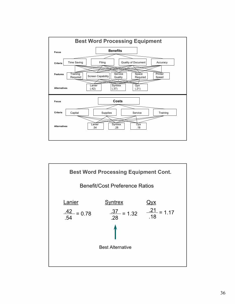
Time Saving Filing Quality of Document Accuracy
TrainingRequired Screen Capability
ServiceQuality
SpaceRequired
PrinterSpeed
Benefits
Lanier(.42)
Syntrex(.37)
Qyx(.21)
Focus
Criteria
Features
Alternatives
Capital Supplies Service Training
Lanier.54
Syntrex.28
Oyx.18
CostsFocus
Criteria
Alternatives
Best Word Processing Equipment
Best Word Processing Equipment Cont.
Benefit/Cost Preference Ratios
Lanier Syntrex Qyx
.42
.54.37.28
.21
.18= 0.78 = 1.32 = 1.17
Best Alternative

37
Group Decision Makingand the
Geometric MeanSuppose two people compare two apples and provide the judgments for the larger over the smaller, 4 and 3 respectively. So the judgments about the smaller relative to the larger are 1/4 and 1/3.
Arithmetic mean4 + 3 = 7
1/7 ≠ 1/4 + 1/3 = 7/12
Geometric mean√ 4 x 3 = 3.46
1/ √ 4 x 3 = √ 1/4 x 1/3 = 1/ √ 4 x 3 = 1/3.46
That the Geometric Mean is the unique way to combine group judgments is a theorem in mathematics.

38
0.05
0.47
0.10
0.15 0.24
ASSIGNING NUMBERS vs.PAIRED COMPARISONS
• A number assigned directly to an object is at best an ordinal and cannot be justified.
• When we compare two objects or ideas we use the smaller as a unit and estimate the larger as a multiple of that unit.

39
• If the objects are homogeneous and if we have knowledge and experience, paired comparisons actually derive measurements that are likely to be close and that indicate magnitude on a ratio scale.
PROBLEMS OF UTILITY THEORY
1. Utility theory is normative; it pre-scribes technically how “rational behavior” should be rather than looking at how people behave in making decisions.
2. Utility theory regards a criterion as important if it has alternatives well spread on it. Later it adopted AHP prioritization of criteria.

40
3. Alternatives are measured on an interval scale. Interval scale numbers can’t be added or multiplied and are useless in resource allocation and dependence and feedback decisions.
4. Utility theory can only deal with a two-level structures if it is to use interval scales throughout.
5. Alternatives are rated one at a time on standards, and are never compared directly with each other.
6. It’s implementation relies on the concept of lotteries (changed to value functions) which are difficult to apply to real life situations.
7. Until the AHP showed how to do it, utility theory could not cope precisely with intangible criteria.
8. Utility theory has paradoxes.(Allais showed people don’t work

41
WHY IS AHP EASY TO USE?• It does not take for granted the measurements on scales, but asks that scale values be interpreted according to the objectives of the problem.
• It relies on elaborate hierarchic structures to represent decision prob-lems and is able to handle problems of risk, conflict, and prediction.
• It can be used to make direct resource allocation, benefit/cost analysis, resolve conflicts, design and optimize systems.
• It is an approach that describes how good decisions are made rather than prescribes how they should be made.

42
WHY THE AHP IS POWERFUL IN CORPORATE PLANNING
1. Breaks down criteria into manage-able components.
2. Leads a group into making a specific decision for consensus or tradeoff.
3. Provides opportunity to examine disagreements and stimulate discussion and opinion.
4. Offers opportunity to change criteria, modify judgments.
5. Forces one to face the entire problem at once.
6. Offers an actual measurement system. It enables one to estimate relative magnitudes and derive ratio scale priorities accurately.

43
7. It organizes, prioritizes and synthesizes complexity within a rational framework.
8. Interprets experience in a relevant way without reliance on a black box technique like a utility function.
9. Makes it possible to deal with conflicts in perception and in judgment.
w
w
n=
w
w
ww
ww
ww
ww
A
A
AA
n
1
n
1
n
n
1
n
n
1
1
1
n
1
n1
MM
K
MM
K
M
K
A w = n w

44
Theorem: A positive n by n matrix has the ratio formA = (wi/wj) , i,j = 1,...,n, if, and only if, it is consistent.
Theorem: The matrix of ratios A = (wi/wj) is consistent if and only if n is its principal eigenvalueand Aw = nw. Further, w > 0 is unique to within a multiplicative constant.
A is consistent if its entries satisfy the conditionajk = aik/aij.
Theorem: w is the principal eigenvector of a positive matrix A if and only if Ee = λ maxe.
When A is inconsistent we write aij = (wi/wj)εij , E = (εij), eT
= (1,…,1)
When the matrix A is inconsistent we have:
Theorem: λ max ≥ n
Proof: Using aji = 1/aij, and Aw = λ maxw, we have
λmax- n = (1/n) ∑ [δ 2 ij / (1+ δ ij )] ≥ 0
1≤i≤ j ≤n
where aij = (1+ δ ij )(wi / wj) , δ ij > -1

45
w = w a ijij
n
1 =j λmax∑
1 = wi
n
1=i∑
aji=1/ aij
w(s) = dt w(t)t)K(s, b
a
λmax∫
w(s)= t)w(t)dtK(s, b
a∫λ
1 = w(s)dsb
a∫
46
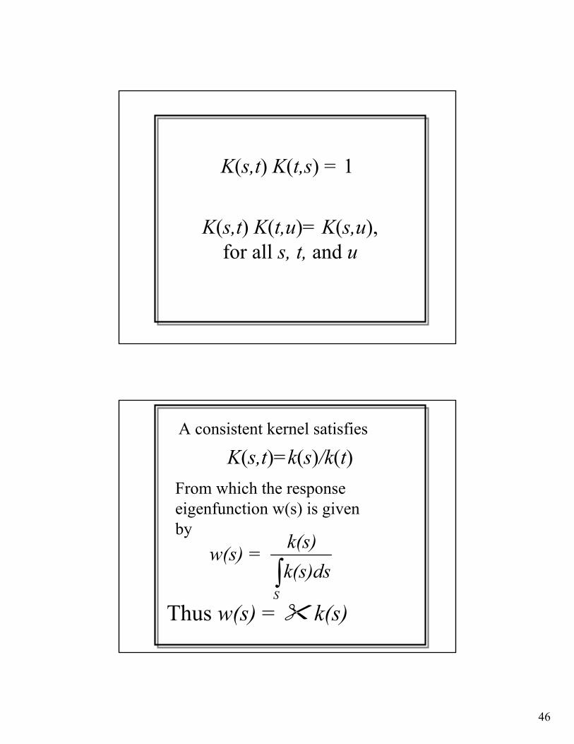
K(s,t) K(t,s) = 1
K(s,t) K(t,u)= K(s,u), for all s, t, and u
A consistent kernel satisfies
K(s,t)=k(s)/k(t)
k(s)dsk(s) = w(s)
S∫
Thus w(s) = k(s)
From which the response eigenfunction w(s) is givenby
47
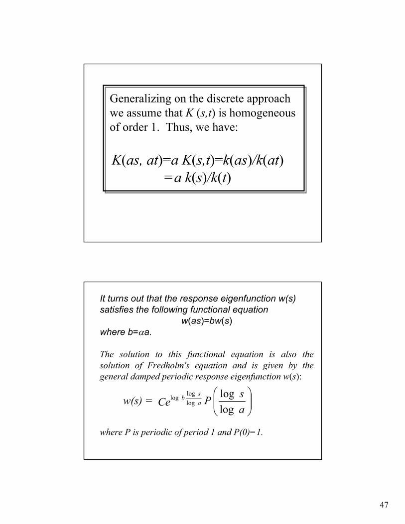
K(as, at)=a K(s,t)=k(as)/k(at)=a k(s)/k(t)
Generalizing on the discrete approach we assume that K (s,t) is homogeneous of order 1. Thus, we have:
It turns out that the response eigenfunction w(s) satisfies the following functional equation
w(as)=bw(s)where b=αa.
The solution to this functional equation is also the solution of Fredholm’s equation and is given by the general damped periodic response eigenfunction w(s):
where P is periodic of period 1 and P(0)=1.
a
s P Ce = w(s) a s b
loglog
logloglog

48
The well-known Weber Fechner logarithmic law of response to stimuli can be obtained as a first order approximation to our eigenfunction:
v(u)=C1 e-βu P(u) ≈ C2 log s+ C3
where P(u) is periodic of period 1, u=log s/log a and log ab -β, β>0.
0a b,+ s a = M ≠log
r)+(1s=sss+s=s+s=s0
0000001
∆∆
The integer valued scale can be derived from the Weber-Fechner Law as follows
α 20
201112 s)r+(1s = r)+(1s = s+s = s ≡∆
2,...) 1, 0, = (n s = s = s n01-nn αα
α s -s = n 0n
log)log(log

49
M1 = a log α, M2 = 2a log α,... , Mn = na log α.
We take the ratios Mi/ M1 , i=1,…,n of the responses:
thus obtaining the integer values of the Fundamental scale of the AHP: 1, 2, …,n.
98
The next step is to provide a framework to represent synthesis of derived scales in the case of feedback.

50
99
The Analytic Network Process (ANP)for Decision Making and Forecasting
with Dependence and Feedback• With feedback the alternatives depend on the criteria as
in a hierarchy but may also depend on each other.
• The criteria themselves can depend on the alternativesand on each other as well.
• Feedback improves the priorities derived from judgments and makes prediction much more accurate.
100
Linear Hierarchy
component,cluster(Level)
element
A loop indicates that eachelement depends only on itself.
Goal
Subcriteria
Criteria
Alternatives
51
101
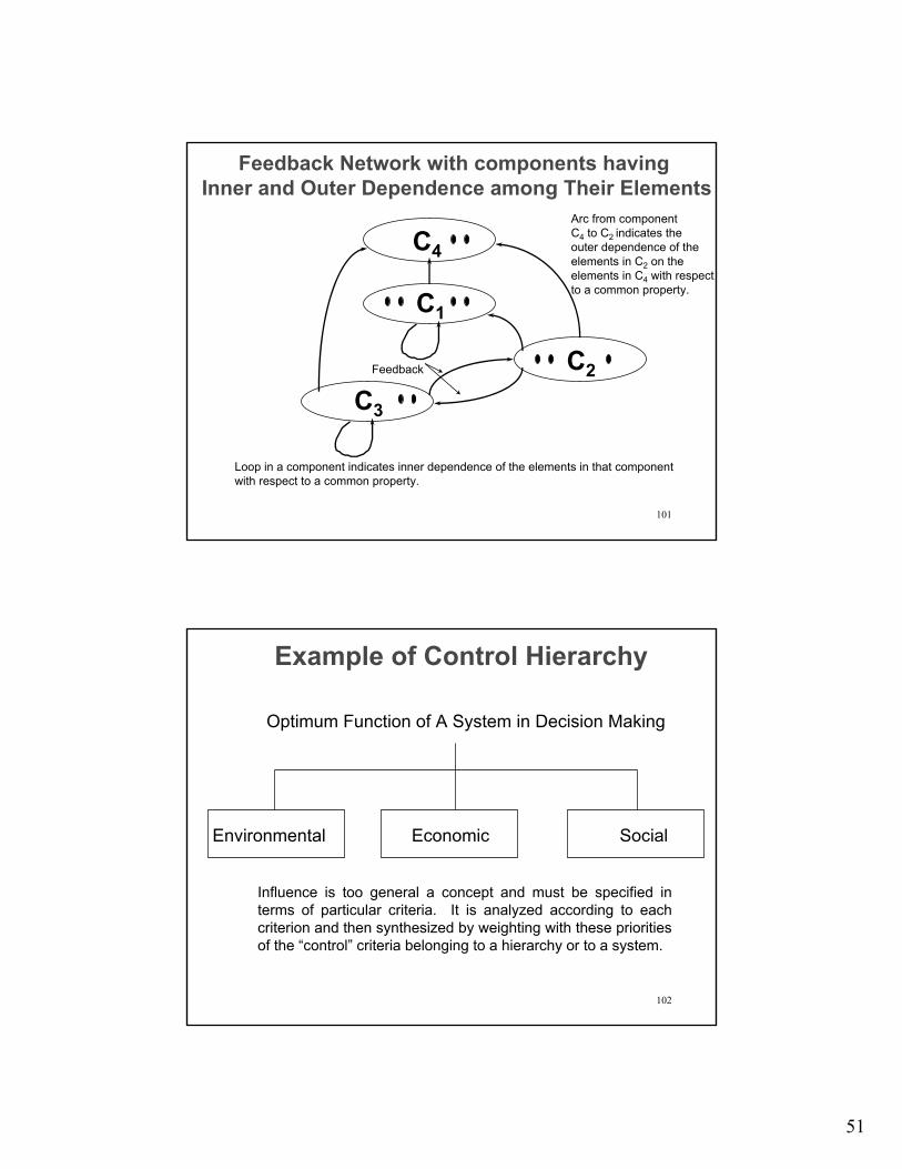
Feedback Network with components having Inner and Outer Dependence among Their Elements
C4
C1
C2
C3
Feedback
Loop in a component indicates inner dependence of the elements in that componentwith respect to a common property.
Arc from componentC4 to C2 indicates theouter dependence of the elements in C2 on theelements in C4 with respectto a common property.
102
Example of Control Hierarchy
Optimum Function of A System in Decision Making
Environmental Economic Social
Influence is too general a concept and must be specified in terms of particular criteria. It is analyzed according to each criterion and then synthesized by weighting with these priorities of the “control” criteria belonging to a hierarchy or to a system.

52
103
Networks and the SupermatrixC1 C2 CN
e11e12 e1n1e21e22 e2n2
eN1eN2 eNnN
W11 W12 W1N
W21 W22 W2N
WN1 WN2 WNN
W =
C1
C2
CN
e11e12
e1n1e21e22
e2n2eN1eN2
eNuN
104
where
Wi1 Wi1 Wi1
Wij =
(j1) (j2) (jnj)
(j1) (j2) (jnj)Wi2 Wi2 Wi2
WiniWini
Wini
(j1) (j2) (jnj)

53
Predicted Turnaround Date of U.S. Economy from April 2001
106
Supermatrix of a Hierarchy
0 0 0 0 0 0
W21 0 0 0 0 0W =
Wn-1, n-2 0 00 0 0 0 Wn, n-1 I
0 W32 0 0 0 0
0 0 0

54
107
Wk=
Wn,n-1 Wn-1,n-2 W32 W21 Wn,n-1 Wn-1,n-2 W32
for k n
Wn,n-1 Wn-1,n-2 Wn,n-1 I
00
0
00
0
00
0
00
0
00
0
… ...
Hierarchic Synthesis
108
The Management of a Water Reservoir
Here we are faced with the decision to choose one of the possibilities of maintaining the water level in a dam at: Low (L), Medium (M) or High (H) depending on the relative importance of Flood Control (F), Recreation (R) and the generation of Hydroelectric Power (E) respectively for the three levels. The first set of three matrices gives the prioritization of the alternatives with respect to the criteria and the second set, those of the criteria in terms of the alternatives.

55
109
A Feedback System with Two Components
Flood Recreation Hydro-Control Electric
Power
Low Intermediate HighLevel Level Level
110
1) Which level is best for flood control?
3) Which level is best for power generation?
2) Which level is best for recreation?
Flood Control
Low Med HighLowMediumHigh
Eigenvector
Consistency Ratio = .107
1 5 7 .7221/5 1 4 .2051/7 1/4 1 .073
Low Med HighLowMediumHigh
Eigenvector
Consistency Ratio = .056
1 1/7 1/5 .0727 1 3 .6495 1/3 1 .279
Recreation
Low Med HighLowMediumHigh
Eigenvector
Consistency Ratio = .101
1 1/5 1/9 .0585 1 1/5 .2079 5 1 .735
Power Generation

56
111
1) At Low Level, which attribute is satisfied best?
2) At Intermediate Level, which attribute is satisfied best?
3) At High Level, which attribute is satisfied best?
Low Level DamF R E Eigenvector
Flood Control 1 3 5 .637Recreation 1/3 1 3 .258Hydro-Electric 1/5 1/3 1 .105
PowerConsistency Ratio = .033
Intermediate Level DamF R E Eigenvector
Flood Control 1 1/3 1 .200Recreation 3 1 3 .600Hydro-Electric 1 1/3 1 .200
PowerConsistency Ratio = .000
High Level DamF R E Eigenvector
Flood Control 1 1/5 1/9 .060Recreation 5 1 1/4 .231Hydro-Electric 9 4 1 .709
PowerConsistency Ratio = .061
112
Hamburger ModelEstimating Market Share of Wendy’s, Burger King and McDonald’s
with respect to the single economic control criterion

57
113
Local: Menu Cleanliness
Speed Service Location Price Reputation
TakeOut
Portion Taste Nutrition
Frequency
Promotion
Creativity
Wendy’s BurgerKing
McDon-ald’s
Menu Item 0.0000 0.0000 0.0000 0.0000 0.0000 0.0000 0.1930 0.0000 0.0000 0.0000 0.0000 0.3110 0.1670 0.1350 0.1570 0.0510 0.1590Cleanliness 0.6370 0.0000 0.0000 0.5190 0.0000 0.0000 0.2390 0.0000 0.0000 0.0000 0.0000 0.0000 0.0000 0.0000 0.2760 0.1100 0.3330Speed 0.1940 0.7500 0.0000 0.2850 0.0000 0.0000 0.0830 0.2900 0.0000 0.0000 0.0000 0.0000 0.0000 0.0000 0.0640 0.1400 0.0480Service 0.0000 0.0780 0.1880 0.0000 0.0000 0.0000 0.0450 0.0550 0.0000 0.0000 0.0000 0.0000 0.0000 0.0000 0.0650 0.1430 0.0240Location 0.0530 0.1710 0.0000 0.0980 0.0000 0.5000 0.2640 0.6550 0.0000 0.0000 0.0000 0.1960 0.0000 0.7100 0.1420 0.2240 0.1070Price 0.1170 0.0000 0.0000 0.0000 0.0000 0.0000 0.0620 0.0000 0.8570 0.0000 0.0000 0.0000 0.8330 0.0000 0.0300 0.2390 0.0330Reputation 0.0000 0.0000 0.0810 0.0980 0.0000 0.0000 0.0570 0.0000 0.0000 0.0000 0.0000 0.4930 0.0000 0.1550 0.2070 0.0420 0.2230Take-Out 0.0000 0.0000 0.7310 0.0000 0.0000 0.5000 0.0570 0.0000 0.1430 0.0000 0.0000 0.0000 0.0000 0.0000 0.0590 0.0510 0.0740Portion 0.2290 0.0000 0.0000 0.0000 0.0000 0.8330 0.2800 0.0000 0.0000 0.0000 0.0000 0.0000 0.0000 0.0000 0.0940 0.6490 0.5280Taste 0.6960 0.0000 0.0000 0.0000 0.0000 0.0000 0.6270 0.0000 0.0000 0.0000 0.0000 0.0000 0.0000 0.0000 0.2800 0.0720 0.1400Nutrition 0.0750 0.0000 0.0000 0.0000 0.0000 0.1670 0.0940 0.0000 0.0000 0.0000 0.0000 0.0000 0.0000 0.0000 0.6270 0.2790 0.3320Frequency 0.7500 0.0000 0.0000 0.0000 0.0000 0.1670 0.5500 0.0000 0.0000 0.0000 0.0000 0.0000 0.6670 0.8750 0.6490 0.7090 0.6610Promotion 0.1710 0.0000 0.0000 0.0000 0.0000 0.8330 0.3680 0.0000 0.0000 0.0000 0.0000 0.5000 0.0000 0.1250 0.0720 0.1130 0.1310Creativity 0.0780 0.0000 0.0000 0.0000 0.0000 0.0000 0.0820 0.0000 0.0000 0.0000 0.0000 0.5000 0.3330 0.0000 0.2790 0.1790 0.2080Wendy's 0.3110 0.5000 0.0990 0.5280 0.0950 0.0950 0.1010 0.1960 0.2760 0.6050 0.5940 0.0880 0.0880 0.1170 0.0000 0.1670 0.2000Burger King 0.1960 0.2500 0.3640 0.1400 0.2500 0.2500 0.2260 0.3110 0.1280 0.1050 0.1570 0.1950 0.1950 0.2680 0.2500 0.0000 0.8000McDonald’s 0.4930 0.2500 0.5370 0.3330 0.6550 0.6550 0.6740 0.4940 0.5950 0.2910 0.2490 0.7170 0.7170 0.6140 0.7500 0.8330 0.0000
Hamburger Model Supermatrix
Cluster: Quality Advertising Competition OtherQuality 0.000 0.000 0.066 0.066Advertising 0.000 0.622 0.533 0.607Competition 0.500 0.247 0.215 0.129Other 0.500 0.131 0.187 0.198
Cluster Priorities Matrix
Other
Q
AdComp
Other Quality CompetitionAdvertising
114
Weighted SupermatrixWeighted: Menu Cleanli
nessSpeed Service Location Price Reputa
tionTakeOut
Portion Taste Nutrition
Frequency
Promotion
Creativity
Wendy’s BurgerKing
McDon-ald’s
Menu Item 0.0000 0.0000 0.0000 0.0000 0.0000 0.0000 0.0382 0.0000 0.0000 0.0000 0.0000 0.0407 0.0219 0.0177 0.0293 0.0095 0.0297Cleanliness 0.1262 0.0000 0.0000 0.3141 0.0000 0.0000 0.0473 0.0000 0.0000 0.0000 0.0000 0.0000 0.0000 0.0000 0.0516 0.0205 0.0622Speed 0.0384 0.4544 0.0000 0.1725 0.0000 0.0000 0.0164 0.1755 0.0000 0.0000 0.0000 0.0000 0.0000 0.0000 0.0120 0.0261 0.0090Service 0.0000 0.0473 0.1138 0.0000 0.0000 0.0000 0.0089 0.0333 0.0000 0.0000 0.0000 0.0000 0.0000 0.0000 0.0121 0.0267 0.0045Location 0.0105 0.1036 0.0000 0.0593 0.0000 0.0990 0.0523 0.3964 0.0000 0.0000 0.0000 0.0257 0.0000 0.0930 0.0265 0.0418 0.0200Price 0.0232 0.0000 0.0000 0.0000 0.0000 0.0000 0.0123 0.0000 0.4287 0.0000 0.0000 0.0000 0.1091 0.0000 0.0056 0.0446 0.0062Reputation 0.0000 0.0000 0.0490 0.0593 0.0000 0.0000 0.0113 0.0000 0.0000 0.0000 0.0000 0.0646 0.0000 0.0203 0.0387 0.0078 0.0417Take-Out 0.0000 0.0000 0.4426 0.0000 0.0000 0.0990 0.0113 0.0000 0.0715 0.0000 0.0000 0.0000 0.0000 0.0000 0.0110 0.0095 0.0138Portion 0.0151 0.0000 0.0000 0.0000 0.0000 0.0550 0.0185 0.0000 0.0000 0.0000 0.0000 0.0000 0.0000 0.0000 0.0062 0.0428 0.0348Taste 0.0460 0.0000 0.0000 0.0000 0.0000 0.0000 0.0414 0.0000 0.0000 0.0000 0.0000 0.0000 0.0000 0.0000 0.0185 0.0047 0.0092Nutrition 0.0050 0.0000 0.0000 0.0000 0.0000 0.0110 0.0062 0.0000 0.0000 0.0000 0.0000 0.0000 0.0000 0.0000 0.0413 0.0184 0.0219Frequency 0.4554 0.0000 0.0000 0.0000 0.0000 0.1014 0.3338 0.0000 0.0000 0.0000 0.0000 0.0000 0.4149 0.5444 0.3455 0.3773 0.3519Promotion 0.1038 0.0000 0.0000 0.0000 0.0000 0.5056 0.2233 0.0000 0.0000 0.0000 0.0000 0.3110 0.0000 0.0778 0.0383 0.0601 0.0697Creativity 0.0474 0.0000 0.0000 0.0000 0.0000 0.0000 0.0498 0.0000 0.0000 0.0000 0.0000 0.3110 0.2071 0.0000 0.1485 0.0953 0.1107Wendy's 0.0401 0.1974 0.0391 0.2082 0.0950 0.0123 0.0130 0.0773 0.1381 0.6044 0.5940 0.0217 0.0217 0.0289 0.0000 0.0359 0.0429Burger King 0.0253 0.0987 0.1436 0.0552 0.2500 0.0323 0.0291 0.1226 0.0640 0.1049 0.1570 0.0482 0.0482 0.0662 0.0537 0.0000 0.1718McDonald ‘s 0.0636 0.0987 0.2118 0.1313 0.6550 0.0845 0.0869 0.1948 0.2976 0.2907 0.2490 0.1771 0.1771 0.1517 0.1611 0.1788 0.0000
Synthesized:Global
Menu Cleanliness
Speed Service Location Price Reputation
TakeOut
Portion Taste Nutrition
Frequency
Promotion
Creativity
Wendy’s BurgerKing
McDon-ald’s
Menu Item 0.0234 0.0234 0.0234 0.0234 0.0234 0.0234 0.0234 0.0234 0.0234 0.0234 0.0234 0.0234 0.0234 0.0234 0.0234 0.0234 0.0234Cleanliness 0.0203 0.0203 0.0203 0.0203 0.0203 0.0203 0.0203 0.0203 0.0203 0.0203 0.0203 0.0203 0.0203 0.0203 0.0203 0.0203 0.0203Speed 0.0185 0.0185 0.0185 0.0185 0.0185 0.0185 0.0185 0.0185 0.0185 0.0185 0.0185 0.0185 0.0185 0.0185 0.0185 0.0185 0.0185Service 0.0072 0.0072 0.0072 0.0072 0.0072 0.0072 0.0072 0.0072 0.0072 0.0072 0.0072 0.0072 0.0072 0.0072 0.0072 0.0072 0.0072Location 0.0397 0.0397 0.0397 0.0397 0.0397 0.0397 0.0397 0.0397 0.0397 0.0397 0.0397 0.0397 0.0397 0.0397 0.0397 0.0397 0.0397Price 0.0244 0.0244 0.0244 0.0244 0.0244 0.0244 0.0244 0.0244 0.0244 0.0244 0.0244 0.0244 0.0244 0.0244 0.0244 0.0244 0.0244Reputation 0.0296 0.0296 0.0296 0.0296 0.0296 0.0296 0.0296 0.0296 0.0296 0.0296 0.0296 0.0296 0.0296 0.0296 0.0296 0.0296 0.0296Take-Out 0.0152 0.0152 0.0152 0.0152 0.0152 0.0152 0.0152 0.0152 0.0152 0.0152 0.0152 0.0152 0.0152 0.0152 0.0152 0.0152 0.0152Portion 0.0114 0.0114 0.0114 0.0114 0.0114 0.0114 0.0114 0.0114 0.0114 0.0114 0.0114 0.0114 0.0114 0.0114 0.0114 0.0114 0.0114Taste 0.0049 0.0049 0.0049 0.0049 0.0049 0.0049 0.0049 0.0049 0.0049 0.0049 0.0049 0.0049 0.0049 0.0049 0.0049 0.0049 0.0049Nutrition 0.0073 0.0073 0.0073 0.0073 0.0073 0.0073 0.0073 0.0073 0.0073 0.0073 0.0073 0.0073 0.0073 0.0073 0.0073 0.0073 0.0073Frequency 0.2518 0.2518 0.2518 0.2518 0.2518 0.2518 0.2518 0.2518 0.2518 0.2518 0.2518 0.2518 0.2518 0.2518 0.2518 0.2518 0.2518Promotion 0.1279 0.1279 0.1279 0.1279 0.1279 0.1279 0.1279 0.1279 0.1279 0.1279 0.1279 0.1279 0.1279 0.1279 0.1279 0.1279 0.1279Creativity 0.1388 0.1388 0.1388 0.1388 0.1388 0.1388 0.1388 0.1388 0.1388 0.1388 0.1388 0.1388 0.1388 0.1388 0.1388 0.1388 0.1388Wendy's 0.0435 0.0435 0.0435 0.0435 0.0435 0.0435 0.0435 0.0435 0.0435 0.0435 0.0435 0.0435 0.0435 0.0435 0.0435 0.0435 0.0435Burger King 0.0784 0.0784 0.0784 0.0784 0.0784 0.0784 0.0784 0.0784 0.0784 0.0784 0.0784 0.0784 0.0784 0.0784 0.0784 0.0784 0.0784McDonald’s 0.1579 0.1579 0.1579 0.1579 0.1579 0.1579 0.1579 0.1579 0.1579 0.1579 0.1579 0.1579 0.1579 0.1579 0.1579 0.1579 0.1579
{
Limiting Supermatrix
Relative local weights: Wendy’s= 0.156, Burger King =0.281, and McDonald’s=0.566

58
115
Hamburger ModelSynthesized Local:
Other Menu Item 0.132Cleanliness 0.115Speed 0.104Service 0.040Location 0.224Price 0.138Reputation 0.167Take-Out 0.086
Quality Portion 0.494Taste 0.214Nutrition 0.316
Advertising Frequency 0.485Promotion 0.246Creativity 0.267
Competition Wendy’s 0.156Burger King 0.281McDonald’s 0.566
Synthesized Local Cont’d:
Simple Hierarchy Complex Hierarchy Feedback Actual(Three Level) (Several Levels) Network Market
ShareWendy’s 0.3055 0.1884 0.156 0.1320Burger King 0.2305 0.2689 0.281 0.2857McDonald’s 0.4640 0.5427 0.566 0.5823
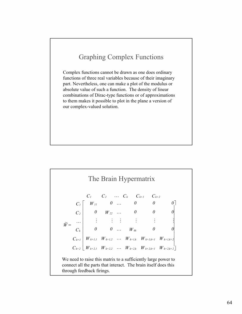
The Brain HypermatrixOrder, Proportionality and Ratio Scales
All order, whether in the physical world or in human thinking, involves proportionality among the parts, to establish harmony and synchrony among them in order to produce the whole. Proportionality means that there is a ratio relation among the parts. Thus, to study order or to create order, we must use ratio scales to capture and synthesize the relations inherent in that order. The question is how? We note that our perceptions of reality are miniaturized in our brains. We control the outside environment, which is much larger than the images we have of it, in a very precise way. This needs proportionality between what our brains perceive and how we interact with the outside world.

59
The Brain Hypermatrix and its Complex Valued Entries
The firings of a neuron are electrical signals. They have both a magnitude and a direction (a modulus and an argument) and are representable in the complex domain. We cannot do them justice by representing them with a real variable. Thus the mathematics of the brain must involve complex variables. The synthesis of signals requires proportionality among them. Such propor-tionality can be represented by a functional equation with a complex argument. Its solution represents the firings of a neuron and is what we want.
Generalizing on the real variable case involving Fredholm’s equation of the second kind we begin with the basic proportionality functional equation:
w( az) = b w(z)whose general solution with a, b and z complex is given by:
w(z) = C b(log z / log a) P(log z / log a)
where P is an arbitrary multi-valued periodic function of period 1.
The Brain Hypermatrix and its Complex Valued Eigenfunction Entries

60
x) - (b)+n(2
i x)-(b) + n(2 + |b|a(
x)-(b) + n(2’aa )(1/2 = n
-
θπδθπ
θππ
∑∞
∞ loglog
whose Fourier transform is given by:
where is the Dirac delta function. In the real situation, the Fourier series is finite as the number of synapses and spines on a dendrite are finite.
x) - (b)+n(2 θπδ
There are three cases to consider in the solution of the functional equation w(az)=bw(z).1) That of real solutions;2) That of complex solutions;3) That of complex analytic solutions.

61
Here is a sketch of how the complex solution is derived. We choose the values of w arbitrarily in the ring between circles around 0 of radii 1(incl.) and |a| (excl.). We designate it by W(z). Thus w(z)=W(z) for 1 ≤ |z| < |a|. By the equation itself, w(z) = w(z/a) b = W(z/a) b for
|a| ≤ |z| < |a|2, w(z) = w(z/a) b = w(z/a2) b2 = W(z/a2) b2
for |a|2 ≤ |z| < |a|3, and so on (also w(z) = w(az)/b = W(az) b-1 for 1/|a| ≤|z| < 1 etc.). Thus the general complex solution of w(az)=bw(z) is given by w(z) = W(z/an) bn for |a|n ≤ |z| < |a|n+1 where W(z) is arbitrary for 1 ≤|z| < |a|. From, |a|n ≤ |z| we have, n = [ log |z| / log |a| ] where
[ x ] is the integer closest to x from below. Here logarithms of real values are taken, so there are no multiple values to be concerned about. But then the solution becomes
w(z) = W( z/ a[ log |z| / log |a| ]) b[ log |z| / log |a| ],
with W arbitrary on the ring 1 ≤ |z| < |a|
Weierstrass’ trigonometric approximation theorem: Any complex-valued continuous function f(x) with period 2π can be approximated uniformly by a sequence of trigonometric polynomials of the form Σ cn einx .
n
A function is called a periodic testing function if it is periodicand infinitely smooth. The space of all periodic testing functions with a fixed common period T is a linear space.A distribution f is said to be periodic if there exists a positivenumber T such that f(t) = f(t-T) for all T. This means thatfor every testing function φ (f(t), φ(t)) = ( f(t-T), φ(t)) .
Sobolev considered a Banach space of functions that are bothLebesgues integrable of class p≥ 1 and differentiable up to a certain order l and under certain conditions on p and l,also continuous.

62
Werner (1970) has shown that(1) Every f(x) ε C[a,b] has a best [T-norm] approximation in En.(2) If the best approximation to f(x) ε C[a,b] in En also belongsto En
0 , then it is the unique best approximation. n
A set of functions of the form ∑ ck fk (x), where ck, k=1,…,n, k=1
are arbitrary reals and n=1,2,…, is dense in C[a,b], if the set of functions {f (x)} is closed in C[a,b], i.e., all its limit points belongto C[a,b]. Muntz proved that the set {s αk },, αk≥0,k=1,2,…} is closed in C[a,b] if and only if ∑ (1/ αk) diverges. Let t=-logs, it follows that the set e-β
kt , βk ≥0, k=1,2,…} is closed in C[0,∞] if and only if
∑ (1/ βk) diverges. It can be shown that the set of products { s αk e-β
kt } is also closed in C[0,∞] with the same two conditions.
Thus finite linear combinations of these functions are dense in C[0,∞].
The justification for the use of the gamma-like response functions { s αk e-β
kt }is partly theoretical and partly empirical.
With the basic assumption that the decay of depolarizationbetween impinging subthreshold impulses is negligible, the distribution of neuronal firing intervals in spontaneous activityhas been approximated by the gamma distribution. If the decay is not negligible as we assume in our work, then onecan decompose the approximation into sums of exponentials as follows: n
En0 = {f(x) | f(x)=∑ cj e λj
x ,, cj ,, λj ε R}j=1
However En0 is not closed under the Tchebycheff or T-norm
||f(x)|| = max | f(x) |x
and hence a best approximation need not exist.
63
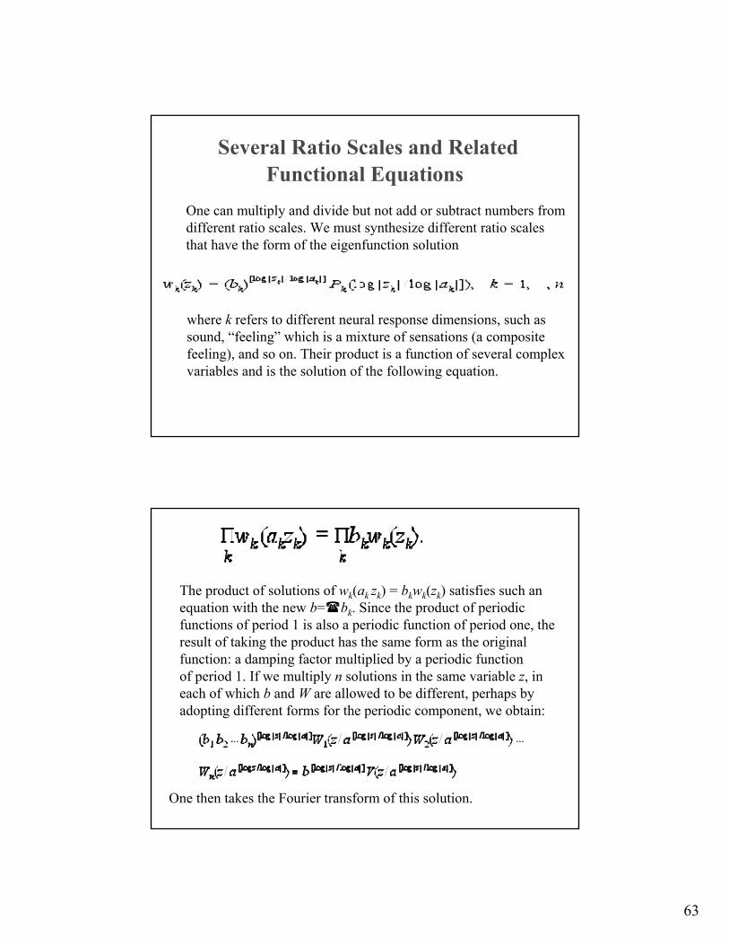
Several Ratio Scales and Related Functional Equations
One can multiply and divide but not add or subtract numbers fromdifferent ratio scales. We must synthesize different ratio scales that have the form of the eigenfunction solution
where k refers to different neural response dimensions, such as sound, “feeling” which is a mixture of sensations (a composite feeling), and so on. Their product is a function of several complex variables and is the solution of the following equation.
The product of solutions of wk(ak zk) = bkwk(zk) satisfies such an equation with the new b= bk. Since the product of periodic functions of period 1 is also a periodic function of period one, the result of taking the product has the same form as the original function: a damping factor multiplied by a periodic function of period 1. If we multiply n solutions in the same variable z, in each of which b and W are allowed to be different, perhaps by adopting different forms for the periodic component, we obtain:
One then takes the Fourier transform of this solution.
64
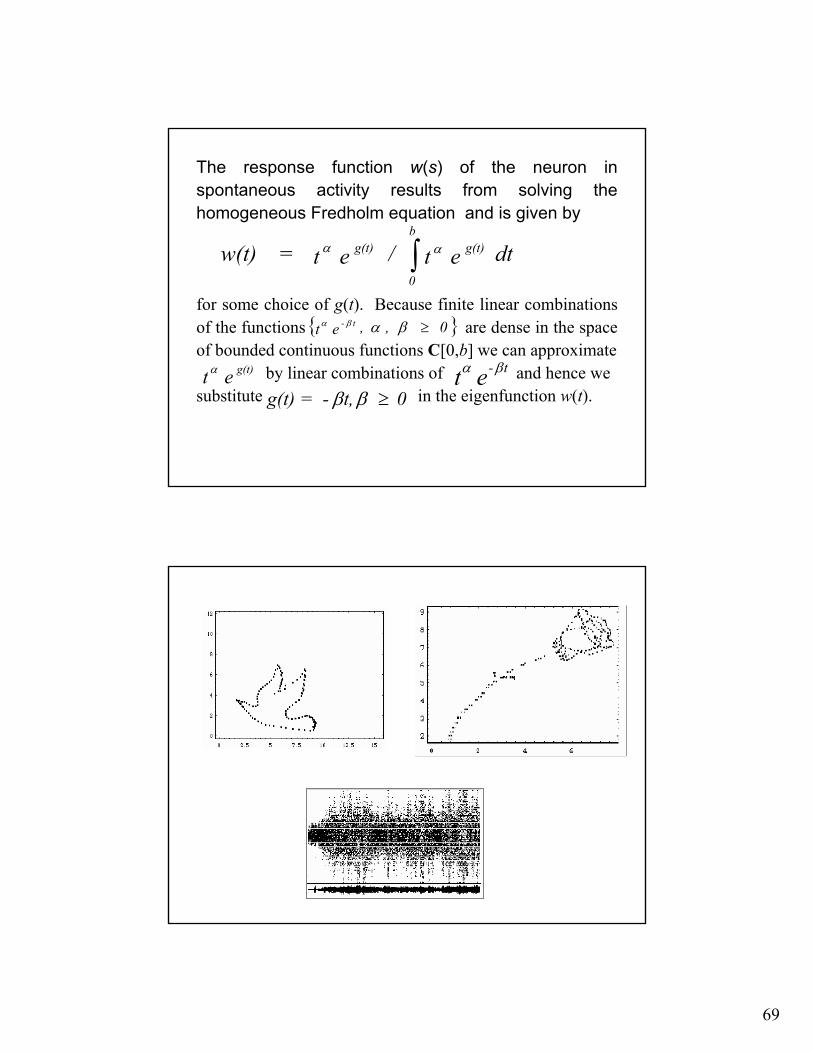
Graphing Complex Functions
Complex functions cannot be drawn as one does ordinaryfunctions of three real variables because of their imaginarypart. Nevertheless, one can make a plot of the modulus or absolute value of such a function. The density of linear combinations of Dirac-type functions or of approximations to them makes it possible to plot in the plane a version of our complex-valued solution.
WWWWW
WWWWW
00W00
000W0
0000W
C
C
C
C
C
= W
C C C C C
2+k2,+k1+k2,+kk2,+k2,2+k2,1+k
2+k1,+k1+k1,+kk1,+k1,2+k1,1+k
kk
22
11
2+k
1+k
k
2
1
2+k1+kk21
K
K
K
MMMMMM
K
K
K
K
~
The Brain Hypermatrix
We need to raise this matrix to a sufficiently large power toconnect all the parts that interact. The brain itself does thisthrough feedback firings.

65
Rods
Cones
Horizontal Cells
Bipolar Cells
Amacrine Cells
Rod
s
Con
es
Hor
izon
tal
Bip
olar
Am
acrin
e
EYEHierarchy
EYEHierarchy
Ganglion Cells(optic nerve)
Gan
glio
n
Layer 1
LATERAL GENICULATEHierarchy
CORTEXHierarchy
(Four types of neurons: Simple, Complex, Hypercomplex,
Higher-order hypercomplex)
LATERALGENICULATE
Hierarchy
CORTEXHierarchy
(Four types of neurons: Simple,
Complex, Hypercomplex,
Higher-order hypercomplex)
Layer 2
Layer 3
Layer 4
Layer 5
Layer 6
Layer 1
Layer 2
Layer 3
Layer 4
Layer 5
Layer 6
Laye
r 1
Laye
r 2
Laye
r 3
Laye
r 4
Laye
r 5
Laye
r 6
Laye
r 1
Laye
r 2
Laye
r 3
Laye
r 4
Laye
r 5
Laye
r 6
Ret
ina
Retina

66
• Since our solution is a product of two factors, the inverse transform can be obtained as the convolution of two functions, the inverse Fourier transform of each of which corresponds to just one of the factors.
• Now the inverse Fourier transform of is given by
Also because of the above discussion on Fourier series, we have
• whose inverse Fourier transform is:
22
)/2(ξβ
βπ+
ue β−
iku
kk euP πα 2)( ∑
∞
−∞=
=
)2( kk
k πξδα −∑∞
−∞=
• Now the product of the transforms of the two functions is equal to the Fourier transform of the convolution of the two functions themselves which we just obtained by taking their individual inverse transforms.
• We have, to within a multiplicative constant:
• We have already mentioned that this solution is general and is applicable to phenomena requiring relative measurement through ratio scales. Consider the case where
∑∫∑∞
−∞=
+∞
∞−
∞
−∞= −+=
−+−
kk
kk kx
dk 2222 )2()()2(
πββαξ
ξχββπξδα
))(2/1(2/cos)( 2/2/ πππ iuiu eeuuP −+==

67
• Bruce W. Knight adopts the same kind of expression for finding the frequency response to a small fluctuation and more generally using instead. The inverse Fourier transform of is given by: 0,2/cos)( >= − βπβ uCeuw u
−+
+
++
22
22
211
211
2ξ
πβξ
πβ
πβc
π2/iue
• When the constants in the denominator are small relative to we have which we believe is why optics, gravitation (Newton) and electric (Coulomb) forces act according to inverse square laws. This is the same law of nature in which an object responding to a force field must decide to follow that law by comparing infinitesimal successive states through which it passes. If the stimulus is constant, the exponential factor in the general response solution given in the last chapter is constant, and the solution in this particular case would be periodic of period one. When the distance is very small, the result varies inversely with the parameter >0.
ξ 21 /ξc
βξ

68
• The brain generally miniaturizes its perceptions into what may be regarded as a model of what happens outside. To control the environment there needs to be proportionality between the measurements represented in the miniaturized models that arise from the firings of our neurons, and the actual measurements in the real world. Thus our response to stimuli must satisfy the fundamental functional equation F(ax) = bF(x). In other words, our interpretation of a stimulus as registered by the firing of our neurons is proportional to what it would be if it were not filtered through the brain.
w(z)=zln b/ln a P(ln z/ln a) whose space-time Fourier transform is a combination of Dirac distributions. Our solution of Fredholm's equation here is given as the Fourier transform,
)P( Ce = dx e F(x) = )f( xi2-+
-
ωω βωωπ∫∞
∞
69
dtet / et = w(t) g(t)b
0
g(t) αα ∫
The response function w(s) of the neuron in spontaneous activity results from solving the homogeneous Fredholm equation and is given by
for some choice of g(t). Because finite linear combinations of the functions are dense in the space of bounded continuous functions C[0,b] we can approximate
by linear combinations of and hence we substitute in the eigenfunction w(t).
{ }0 , ,et t- ≥βαβα
et g(t)α et t-βα
0 t,- = g(t) ≥ββ