the application of qualification testing, field … · aerospace report no. atr-2005(7796)-1 the...

AEROSPACE REPORT NO. ATR-2005(7796)-1

The Application of Qualification Testing, Field Testing, and Accelerated Testing for Estimating Long-Term Durability of Composite Materials for Caltrans Applications 25 February 2005 Prepared by G. L. STECKEL and G. F. HAWKINS Space Materials Laboratory Laboratory Operations Prepared for STATE OF CALIFORNIA DEPARTMENT OF TRANSPORTATION Sacramento, CA 94273 Contract No. 59A0188 Engineering and Technology Group PUBLIC RELEASE IS AUTHORIZED EL SEGUNDO, CALIFORNIA

LABORATORY OPERATIONS

The Aerospace Corporation functions as an “architect-engineer” for national security programs, specializing in advanced military space systems. The Corporation's Laboratory Operations supports the effective and timely development and operation of national security systems through scientific research and the application of advanced technology. Vital to the success of the Corporation is the technical staff’s wide-ranging expertise and its ability to stay abreast of new technological developments and program support issues associated with rapidly evolving space systems. Contributing capabilities are provided by these individual organizations:

Electronics and Photonics Laboratory: Microelectronics, VLSI reliability, failure analysis, solid-state device physics, compound semiconductors, radiation effects, infrared and CCD detector devices, data storage and display technologies; lasers and electro-optics, solid-state laser design, micro-optics, optical communications, and fiber-optic sensors; atomic frequency standards, applied laser spectroscopy, laser chemistry, atmospheric propagation and beam control, LIDAR/LADAR remote sensing; solar cell and array testing and evaluation, battery electrochemistry, battery testing and evaluation. Space Materials Laboratory: Evaluation and characterizations of new materials and processing techniques: metals, alloys, ceramics, polymers, thin films, and composites; development of advanced deposition processes; nondestructive evaluation, component failure analysis and reliability; structural mechanics, fracture mechanics, and stress corrosion; analysis and evaluation of materials at cryogenic and elevated temperatures; launch vehicle fluid mechanics, heat transfer and flight dynamics; aerothermodynamics; chemical and electric propulsion; environmental chemistry; combustion processes; space environment effects on materials, hardening and vulnerability assessment; contamination, thermal and structural control; lubrication and surface phenomena. Microelectromechanical systems (MEMS) for space applications; laser micromachining; laser-surface physical and chemical interactions; micropropulsion; micro- and nanosatellite mission analysis; intelligent microinstruments for monitoring space and launch system environments. Space Science Applications Laboratory: Magnetospheric, auroral and cosmic-ray physics, wave-particle interactions, magnetospheric plasma waves; atmospheric and ionospheric physics, density and composition of the upper atmosphere, remote sensing using atmospheric radiation; solar physics, infrared astronomy, infrared signature analysis; infrared surveillance, imaging and remote sensing; multispectral and hyperspectral sensor development; data analysis and algorithm development; applications of multispectral and hyperspectral imagery to defense, civil space, commercial, and environmental missions; effects of solar activity, magnetic storms and nuclear explosions on the Earth’s atmosphere, ionosphere and magnetosphere; effects of electromagnetic and particulate radiations on space systems; space instrumentation, design, fabrication and test; environmental chemistry, trace detection; atmospheric chemical reactions, atmospheric optics, light scattering, state-specific chemical reactions, and radiative signatures of missile plumes.

1. REPORT NO.

CA/ES-ATR-2005-7796-12. GOVERNMENT ACCESSION NO. 3. RECIPIENT’S CATALOG NO.

4. TITLE AND SUBTITLE

The Application of Qualification Testing, Field Testing, andAccelerated Testing for Estimating Long-Term Durability ofComposite Materials for Caltrans Applications

5. REPORT DATE

25 February 2005

6. PERFORMING ORGANIZATION CODE

7. AUTHOR(S)

G. L. Steckel and G. F. Hawkins8. PERFORMING ORGANIZATION REPORT NO.

ATR-2005(7796)-1

9. PERFORMING ORGANIZATION NAME AND ADDRESS

The Aerospace CorporationP.O. Box 92957Los Angeles CA 90009

10. WORK UNIT NO.

11. CONTRACT OR GRANT NO.

59A0188

12. SPONSORING AGENCY NAME AND ADDRESS

State of CaliforniaDepartment of TransportationSacramento, CA. 94273-0001

13. TYPE OF REPORT & PERIOD COVERED

Final Report

14. 14. SPONSORING AGENCY CODE

15. SUPPLEMENTARY NOTES

16. ABSTRACT

Caltrans has begun utilizing composite materials in several bridge applications. Formal procedures for the evaluationand qualification of composite casings for seismic retrofit of bridge columns were adopted in 1995 and are being appliedby Caltrans to all structural applications of composite materials. Environmental durability testing to ensure the long-term integrity of composite structures is an integral part of the qualification process. The Aerospace Corporation sup-ported Caltrans in the development of qualiication requirements and test procedures, and conducted durability testing oncandidate systems for the composite casings for seismic retrofit application. More recently, Caltrans contracted withAerospace to perform qualification durability testing on composite materials used in the construction of the King’sStormwater Bridge and to conduct research activities related to the durability of composites for infrastructure applica-tions. Research areas included a field durability study conducted at the Yolo Causeway to help define the field environ-ment, and to compare durability in the field environment with the results of the qualification test program. A short-coming of the qualification program was the inability to make long-term (30−50 yr) tensile strength projections from therelatively short-term (1.14 yr) exposure data for those systemsthat showed susceptibility in moist environments. Post-exposure tensile strength data from accelerated exposures at an elevated temperature and significantly longer term (6.3yr) laboratory exposures under the qualification conditions were combined with the qualification test data to developexpressions for making long-term tensile strength projections under service conditions.

17. KEY WORDS

Composites, Infrastructure, Seismic Retrofit,Durability

18. DISTRIBUTION STATEMENT

No Restrictions. This document is availablethrough the National Technical InformationService, Springfield, VA 22161

19. SECURITY CLASSIF. (OF THIS REPORT)

Unclassified

20. SECURITY CLASSIF. (OF THIS PAGE)

Unclassified

21. NO. OF PAGES

89

22. PRICE

AEROSPACE REPORT NO. ATR-2005(7796)-1

THE APPLICATION OF QUALIFICATION TESTING, FIELD TESTING, AND ACCELERATED TESTING FOR ESTIMATING LONG-TERM

DURABILITY OF COMPOSITE MATERIALS FOR CALTRANS APPLICATIONS

Prepared by

G. L. STECKEL and G. F. HAWKINS Space Materials Laboratory

Laboratory Operations

25 February 2005

Engineering and Technology Group THE AEROSPACE CORPORATION

El Segundo, CA 90245-4691

Prepared for

STATE OF CALIFORNIA DEPARTMENT OF TRANSPORTATION

Sacramento, CA 94273

Contract No. 59A0188

PUBLIC RELEASE IS AUTHORIZED

Abstract

Caltrans has begun utilizing composite materials in several bridge applications, including girders and decks on new bridges, replacement decks and seismic retrofit of columns on old bridges, and for general structural reinforcement. Formal procedures for the evaluation and qualification of composite casings for seismic retrofit of bridge columns were adopted in 1995 and are being applied by Caltrans to all structural applications of composite materials. Environmental durability testing to ensure the long-term integrity of composite structures is an integral part of the qualification process. The Aerospace Corporation supported Caltrans in the development of quali-fication requirements and test procedures, and conducted durability testing on candi-date systems for the composite casings for seismic retrofit application. More recently, Caltrans contracted with Aerospace to perform qualification durability test-ing on composite materials used in the construction of the King’s Stormwater Bridge and to conduct research activities related to the environmental durability of compos-ites for infrastructure applications. Research areas included a field durability study conducted at the Yolo Causeway to help define the field environment through humidity, pH, and temperature sensors, and to compare durability in the field envi-ronment with the results of the qualification test program. A shortcoming of the qualification durability test program was the inability to make long-term (30−50 yr) tensile strength projections from the relatively short-term (1.14 yr) laboratory expo-sure data for those systems, chiefly E-glass-reinforced composites, that showed sus-ceptibility in moist environments. Post-exposure tensile strength data from acceler-ated exposures at an elevated temperature and significantly longer term (6.3 yr) labo-ratory exposures under the qualification conditions were combined with the qualifi-cation test data to develop expressions for making long-term tensile strength projec-tions under service conditions.

iii

Acknowledgments

The authors wish to acknowledge the support of the following individuals:

• Li-Hong Sheng (Caltrans) for program guidance throughout this effort

• Ben Nelson for monitoring environmental exposures and conducting ten-sile tests and lap shear strength tests

• Bruce Weiller for selection and validation of sensors for field environ-ment monitoring

• Paul Chaffee for construction of waterproof sensor chambers

• Ben Nelson, George Panos, and Oscar Esquivel for mounting composite panels and sensors on columns at the Yolo Causeway

• Jack Shaffer for editing and preparing this report for publication

iv

Note

The SEH 51/Tyfo S E-glass/epoxy composite panels studied in this program were submitted in 1996 to Caltrans for evaluation under the Seismic Retrofit of Bridge Columns Program. At that time, the material was marketed by Hexcel-Fyfe under a joint venture between Hexcel Corporation and Fyfe Company. The material is currently marketed separately by Fyfe Co. as SEH 51/Tyfo S and by Hexcel Corp. as Hex 3R Wrap 107/Hex 3R Epoxy 300. Therefore, all data in this report for SEH 51/Tyfo S also applies to Hex 3R Wrap 107/Hex 3R Epoxy 300.

All trademarks, service marks, and trade names are the property of their respective owners.

v

Contents

1. Durability of Composites for the King’s Stormwater Bridge............................................... 1

1.1 Introduction................................................................................................................. 1

1.2 Experimental Procedures ............................................................................................ 2

1.2.1 Environmental Exposures .............................................................................. 2

1.2.2 Carbon/Epoxy Girder Composite System...................................................... 5

1.2.3 E-glass/Epoxy Vinyl Ester Bridge Deck Composite System......................... 6

1.2.4 Material Property Measurements................................................................... 8

1.3 Results and Discussion for the Carbon/Epoxy Girder Composite .............................. 11

1.3.1 Physical Appearance and Optical Microscopy .............................................. 11

1.3.2 Baseline Properties from Control Panels ....................................................... 12

1.3.3 Effects of Environmental Exposures on Mechanical and Physical Properties 18

1.4 Results and Discussion for the E-glass/Epoxy Vinyl Ester Deck-Reinforcement Composite and Bonded Assemblies............................................................................ 21

1.4.1 Physical Appearance and Optical Microscopy .............................................. 21

1.4.2 Baseline Properties from Control Panels ....................................................... 23

1.4.3 Baseline Lap Shear Strength from Bonded Assemblies ................................ 26

1.4.4 Effects of Environmental Exposures on Mechanical and Physical Properties 27

1.5 Summary and Conclusions ......................................................................................... 32

2. Durability of Composites Exposed to the Yolo Causeway Environment............................. 35

2.1 Introduction................................................................................................................. 35

2.2 Materials and Field Exposure Procedures................................................................... 36

2.3 Testing Procedures...................................................................................................... 39

2.4 Results and Discussion ............................................................................................... 40


3. Environmental Monitoring of Composite Casings at the Yolo Causeway ........................... 51

3.1 Introduction and Background ..................................................................................... 51

vi

3.2 Temperature/Relative Humidity Sensors and Data Acquisition ................................. 51

3.3 Sensor Mounting......................................................................................................... 52



4. Long-Term Durability of E-glass/Polymer Composites ....................................................... 60

4.1 Introduction and Background ..................................................................................... 61

4.2 Experimental Procedures ............................................................................................ 61



References ...................................................................................................................................... 70

Appendix 1—Tabulated Data for Individual Tensile, SBSS, and Hardness Measurements for the Kings Stormwater Bridge Carbon/Epoxy Girder Composite....................... 73

Appendix 2—Tabulated Data for Individual Tensile, Hardness, and Bondline LSS Measurements for the Kings Stormwater Bridge E-glass/Epoxy Vinyl Ester Deck-Reinforcement Composite .......................................................... 83

Figures

1.1. Photograph of MMC pultruded bridge deck sections........................................................ 1

1.2. Photograph of ATK flat panels and ring segments. .......................................................... 5

1.3. Photograph of MMC bonded assembly and LSS samples. ............................................... 7

1.4. Drawing for preparation of single lap shear samples from bonded composite panel assemblies.......................................................................................................................... 10

1.5. Micrograph of cross section normal to axial direction of carbon/epoxy ring segment exposed to freeze/thaw exposure. ................................................................ 12

1.6. Micrograph of cross section normal to fiber direction of carbon/epoxy Panel No. A03-1M after 10,000 h alkali exposure. ........................................................... 12

1.7. Micrograph of cross section normal to fiber direction of carbon/epoxy Panel No. A03-2M after weathering exposure. ................................................................. 13

vii

1.8. Young’s modulus of carbon/epoxy panels as function of panel fiber content. ................. 14

1.9. Young’s modulus of carbon/epoxy panels as function of panel thickness. ....................... 15

1.10. Stress-strain curve for carbon/epoxy Control Sample No. A01-2M8. .............................. 15

1.11. Moisture absorption curves for 10,000-h carbon/epoxy panels and ring segments. ......... 19

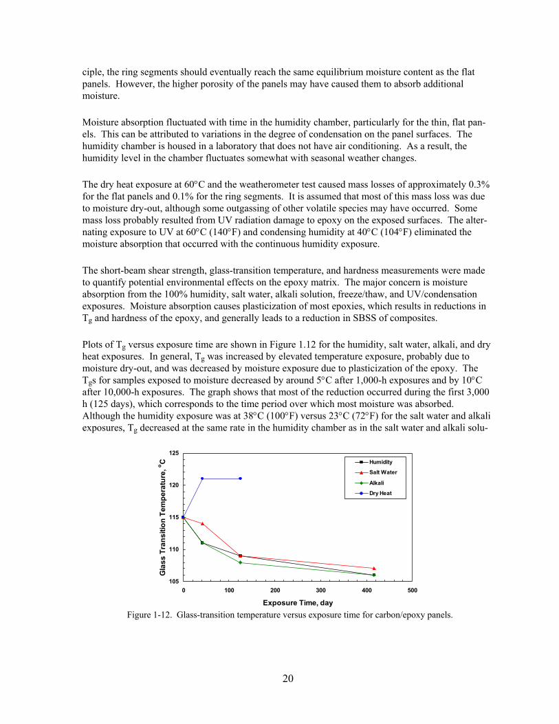
1-12. Glass-transition temperature versus exposure time for carbon/epoxy panels. .................. 20

1.13. Micrograph of cross section normal to 0° direction of E-glass/epoxy vinyl ester control panel. ................................................................................................... 22

1.14. Micrograph of cross section normal to 0° direction of bonded assembly exposed to freeze/thaw exposure....................................................................................... 23

1.15. Stress-strain curve for E-glass/epoxy vinyl ester Control Sample No. C4-1. ................... 25

1.16. Photograph of fractured tensile samples from E-glass/epoxy vinyl ester control panels. . 25

1.17. Stress-strain curve for web section of Duraspan 766 pultrusion. .................................. 25

1.18. Moisture absorption curves for fiberglass panels and bonded assemblies. ....................... 28

1.19. Loss modulus versus temperature for E-glass/epoxy vinyl ester control and exposure panels........................................................................................................... 30

1.20. Young’s modulus versus Tg for E-glass/epoxy vinyl ester control and exposure panels. . 30

1.21. Examples of failure modes exhibited by bonded assembly LSS samples. ........................ 31

2.1. Anti-bending fixture for single-lap shear testing............................................................... 40

2.2. Photographs of Fyfe Co. SCH 41/Tyfo S Carbon/Epoxy panels taken at beginning (left) and after 1-yr field exposure ...................................................... 41

2.3. Photographs of Myers Technologies, Inc. E-glass/Polyester/MOR-AD-695-28 Adhesive-bonded assemblies taken at beginning (left) and after 1-yr field exposure. ...................... 41

2.4. Photographs of Mitsubishi Chemical Co. carbon/epoxy Panel No. M2-2L22A after 4-yr field exposure. ................................................................................................... 42

2.5. Optical micrographs of Master Builders, Inc. laboratory control panel and 2-yr Yolo Causeway exposure panel. ................................................................................................ 44

2.6. Fracture surfaces of LSS samples from Myers Technologies, Inc. bonded assemblies. ... 48

3.1. Schematic diagram of sensor attachment to a composite overwrapped column. .............. 52

3.2. Temperature and relative humidity for the casing middle on Bent 178 Column 8. .......... 55

viii

3.3. Typical temperature and relative humidity data from the casing top on Bent 177 Column 7 during five days in the summer of 1999....................................... 55

3.4. Temperature and relative humidity data from the casing middle on Bent 178 Column 3 and Column 8. .............................................................................. 56

3.5. 31-day running average relative humidity and temperature for all six sensors. ................ 57

4.1. Retained tensile strength versus Log of exposure time in 100% humidity or salt water for SEH 51/Tyfo S. ..................................................................................... 63

4.2. Retained tensile strength versus Log of exposure time in 100% humidity or salt water for E-glass/vinyl ester. .................................................................................. 64

4.3. Retained tensile strength versus Log of exposure time in 100% humidity or salt water for E-glass/polyester. .................................................................................... 65

4.4. Retained tensile strength as a function of exposure time at 23, 38, and 70°C for SEH 51/Tyfo S......................................................................................................................... 68

4.5. Predicted retained tensile strength as a function of exposure time and temperature for SEH 51/Tyfo S........................................................................................................... 68

Tables

1.1. Environmental Durability Test Matrix .............................................................................. 3

1.2. Identification Numbers of ATK Panels and Ring Segments ............................................. 6

1.3. Identification Numbers of MMC Panels and Bonded Assemblies.................................... 8

1.4. Fiber Content and Thickness of Carbon/Epoxy Panels ..................................................... 14

1.5. Normalized Tensile Properties for Carbon/Epoxy Control Panels.................................... 16

1.6. Short Beam Shear Strength for Carbon/Epoxy Control Ring Segments ........................... 17

1.7 Mechanical and Physical Properties of Carbon/Epoxy Composites after Environmental Exposures ......................................................................................... 18

1.8. Tensile Properties for E-glass/Epoxy Vinyl Ester Control Panels .................................... 23

1.9. Tensile Properties for E-glass/Epoxy Vinyl Ester in 90° Direction .................................. 24

1.10. Tensile Properties for Web Section of Duraspan 766 Pultrusion .................................. 25

ix

1.11. LSS Data for Pultrusion/Hand-Lay-up Bonded Assemblies. ............................................ 26

1.12. Mechanical and Physical Properties of E-glass/Epoxy Vinyl Ester after Environmental Exposures ......................................................................................... 28

1.13. LSS Data for Bonded Assemblies After Environmental Exposures ................................. 31

2.1. List of Composite Materials for Yolo Causeway Field Durability Study ......................... 36

2.2. Glass-Fiber-Reinforced Composite Panels........................................................................ 38

2.3. Carbon-Fiber-Reinforced Composite Panels..................................................................... 38

2.4. Mechanical and Physical Properties of Carbon-Fiber-Reinforced Composites ................ 42

4.1. Tensile Properties of SEH 51/Tyfo S after 2,363-day Exposures ................................... 63

4.2. Tensile Properties of E-glass/Vinyl Ester after 2,363-day Exposures............................... 64

4.3. Tensile Properties of E-glass/Polyester after 2,363-day Exposures .................................. 65

4.4. Curve Fit Parameters for Long Term Tensile Strength Predictions .................................. 66

4.5. SEH 51/Tyfo S Tensile Strength Following Deionized Water Exposure at 70°C .......... 67

x

1. Durability of Composites for the King’s Stormwater Bridge

1.1 Introduction The Kings Stormwater Bridge on State Route 86 near the Salton Sea was constructed using concrete-filled carbon/epoxy tubes as girders and an E-glass/polyester/vinyl ester bridge deck. Specifications for the girders and bridge deck, the results of load tests on the bridge, and the results of preliminary durability testing on the girders and deck have been reported by the Division of Structural Engineer-ing, University of California, San Diego (UCSD).1–4 Caltrans requested complete environmental durability testing on the girder and bridge deck materials to be performed by The Aerospace Corpo-ration following the test matrix and test procedures developed for the Seismic Retrofit of Bridge Col-umns Program.5

The carbon/epoxy girders were fabricated by Alliant Techsystems Incorporated (ATK), Bacchus Works, Magna, Utah, by a wet filament winding process. Twelve thousand filament tows of Hex-celTM Corporation’s AS4D carbon fibers were used to reinforce EPONTM 826 epoxy resin with EPI-CURETM 9551 curing agent. EPONTM 826 and EPI-CURETM 9551 are manufactured by Resolution Performance Products, Houston, Texas. The lay-up, starting from the inner wall surface, is one layer of carbon fiber fabric/902/±10/902/±102/902/±102/902/±10/903. Each 90° hoop layer is 0.010 in. (0.25 mm) thick, and each set of ±10° helical plies is 0.040 in. (1.02 mm) thick. Thus, the tubes have a total hoop reinforcement thickness of 0.11 in. (2.79 mm) and a total helical reinforcement thickness of 0.24 in. (6.10 mm). The total wall thickness, including the inner fabric layer, is 0.43 in. (0.89 cm). The carbon/epoxy girders are 32 ft (9.75 m) long and have an inside diameter of 13.5 in. (34.3 cm). They are filled with concrete during the bridge construction process.

The bridge deck materials were fabricated by Martin Marietta Composites, Incorporated (MMC), Raleigh, North Carolina. The deck, MMC’s DuraspanTM 766 modular design, is constructed from interlocking dual-cell sections of pultruded E-glass/Isophthalic polyester composite. Short pieces of a pair of typical pultruded sections are shown in Figure 1.1. The deck sections are reinforced with

Figure 1.1. Photograph of MMC pultruded bridge deck sections.

1

E-glass tows, mats, and fabrics that are supplied by Johnson Industries, BTI. Isophthalic polyester resin (Aropol 7334T-15), supplied by Ashland Chemicals, is the composite matrix. In the pultrusion process, the fiberglass is wetted with polyester resin and pulled through heated dies, which compact and cure the reinforced resin into the precise bridge deck cross section. Deck sections are assembled by bonding the pultruded sections together using a structural urethane adhesive.

For the Kings Stormwater Bridge, the deck was further reinforced by E-glass/epoxy vinyl ester panels that were applied to the upper and lower surfaces of the assembled deck. The flat panels were fabri-cated by hand lay-up procedures using three plies of a triaxial fabric that was also used for the pul-truded deck sections. Each layer of fabric has a [0(50%)/±45(50%)] lay-up. The overall orientation of the plies in the panels is [(0/±45)/(90/±45)/(0/±45)]. The vinyl ester resin was DERAKANE 411-370 manufactured by Dow Chemical Company. The panels were laid up on the assembled deck using wet lay-up procedures with the 0° direction of the panels coincident with the pultrusion direction and with 0° sides of the panels facing outward. Reinhold Industries’ ATPRIME-2 urethane primer was applied to the deck surface prior to the lamination to enhance bonding between the E-glass/Isophthalic polyester deck and E-glass/epoxy vinyl ester reinforcement panels.

The original test plan was to perform environmental durability testing on the carbon/epoxy girder material, the E-glass/Isophthalic polyester pultrusion material, the E-glass/epoxy vinyl ester panels, and the bond between the reinforcement panels and bridge deck. However, Caltrans determined that the reinforcement panels carry significantly higher loads than the pultruded material. Therefore, the pultruded material was omitted from the durability test matrix.

Environmental exposures included 100% humidity at 38°C (100°F), immersion in salt water, immer-sion in an alkali solution, alternating ultraviolet light/condensation, dry heat at 60°C (140°F), a freeze/thaw test, and immersion in diesel fuel. The effects of the environmental exposures were quantified by measurements of the composite panel mass, tensile modulus, tensile strength, tensile failure strain, interlaminar shear strength, and glass-transition temperature. Lap shear strength meas-urements were made on bonded assemblies of the pultruded deck and reinforcement panels to deter-mine the environmental resistance of the adhesive bond. Property measurements were made after exposure intervals of 1,000, 3,000, and 10,000 h (41.7, 125, and 417 days) to allow estimates of deg-radation over the projected service life.

1.2 Experimental Procedures

1.2.1 Environmental Exposures The test matrix of environmental durability exposure conditions required by Caltrans is given in Table 1.1. The carbon/epoxy girder material and E-glass/vinyl ester deck material were subjected to these environmental exposures for the times or numbers of cycles indicated. Each composite panel or bonded assembly was subjected to one exposure condition. Thus, the individual effects of each expo-sure condition were evaluated. Synergism between the different exposures was not evaluated except as indicated in the ultraviolet/condensation and freeze/thaw exposures. Natural or climatic exposures include: water resistance, salt water resistance, weathering resistance, and a cyclic freeze/thaw test. Additional exposures include four hours in diesel fuel to evaluate the effects of a fuel spill following a vehicular accident and an alkali solution exposure to evaluate long-term compatibility between con-

2

crete and the composite systems. The bonded assemblies were not subjected to the UV/condensation or diesel fuel exposures since the adhesive is not exposed to direct sunlight or short-term fuel spills.

For water resistance, 100% humidity at 38°C (100°F) was selected as an accelerated test. This expo-sure is considered more severe than an immersion test at ambient temperature because the elevated temperature increases water absorption and chemical reaction rates, and the high-humidity exposure allows for atmospheric reactions that would not occur in an immersion test. The humidity exposure was performed following the procedures of ASTM D 2247.6 The composite panels were mounted on racks in the humidity chamber and held in a vertical position. The humidity chamber was set up to provide condensation on the panel surfaces.

An immersion test was selected for salt water resistance to test the effects of prolonged immersion in ocean water. Substitute ocean water prepared following ASTM D 11417 was used for the salt water resistance exposure. The composite panels were immersed in 10 liters of substitute ocean water that was maintained in a 36-liter, closed polypropylene container having the approximate inside dimen-sions of 20 x 14 x 6 in. (50 x 35 x 15 cm). All test panels for a given composite system were exposed in a single container, but separate containers were used for different systems. The test panels rested on the bottom of the containers in a horizontal position with adequate gaps between panels to main-tain chemical equilibrium throughout the liquid bath.

The 60°C (140°F) exposure was selected as the maximum exposure temperature anticipated in serv-ice. At the elevated temperature, it was anticipated that any degradation would occur rapidly. There-fore, the maximum exposure time was limited to 3,000 h (125 days). The exposure was carried out following ASTM D 30458 with the panels resting on horizontal racks in a forced-draft circulating air furnace. All composite systems were exposed in the same furnace with a separate rack for each sys-tem.

A standard ultraviolet (UV) resistance test (ASTM G539) was used to simulate weathering effects with alternating exposures to UV and condensing humidity. One side of the composite panels was exposed to cyclic exposures of fluorescent UV light at 60°C (140°F) for 4 h followed by water condensation at 40°C (104°F) for 4 h. Total exposure was for 100 cycles, corresponding to 400-h exposures to UV

Table 1.1. Environmental Durability Test Matrix

Environmental Durability Test

Test Conditions

Test Duration

Water Resistance 100% Humidity At 38°C 1,000, 3,000, & 10,000 h

Salt Water Resistance Immersion At 23°C 1,000, 3,000, & 10,000 h

Alkali Resistance Immersion In CaCO3 pH = 9.5 & 23°C

1,000, 3,000, & 10,000 h

Dry Heat Resistance Furnace At 60°C 1,000 & 3,000 h

Fuel Resistance Immersion At 23°C 4 h

Weathering Resistance Cycle Between UV At 60°C & Condensate At 40°C

4 h per Condition, 100 Cycles

Freeze/Thaw Resistance Cycle Between 100% Humidity At 38°C & Freezer At -18°C

24 h per Cycle, 20 Cycles

3

light and to condensation. This test was intended to simulate the deterioration caused by water as rain or dew and the UV energy in sunlight.

The freeze/thaw test was developed to determine the effects on the composite systems of freezing following significant water absorption. The panels were maintained in the humidity chamber at 100% humidity and 38°C (100°F) for a minimum of two weeks prior to the initial exposure to the freezer at –18°C (0°F). Typically, the panels were placed in the freezer at the beginning of the workday and returned to the humidity chamber at the end of the day. Thus, each 24-h cycle included approxi-mately 9 h in the freezer and 15 h in the humidity chamber. It was anticipated that any effects of the freeze-thaw exposure would become apparent after a few cycles, and the test was performed for only 20 cycles. However, it was recognized that the effects could become more pronounced with addi-tional cycling. Therefore, allowance was made to perform additional freeze/thaw cycles on any com-posite systems showing susceptibility to this exposure.

The alkali resistance test was performed to determine any effect on composite overwraps from the high alkalinity of concrete columns. This is an important test because it is well known that unpro-tected glass fibers10,11 and many organic resins12 are severely degraded in alkaline solutions. A satu-rated solution of calcium carbonate, CaCO3, in water having a pH of 9.5 was selected for this expo-sure. The selection was originally made for the seismic retrofit of bridge columns application in which columns requiring retrofit are at least 20 years old. Concrete reacts with the atmosphere to form CaCO3, and it was anticipated that this would be the appropriate alkaline solution exposure for that application. However, for the King’s Stormwater Channel Bridge application, the carbon/epoxy girders are filled with fresh concrete, which has a much higher alkalinity (pH ≥ 14).13 Therefore, a higher pH exposure may have been more appropriate for the carbon/epoxy composite system. Cal-trans directed Aerospace to use the standard procedure that was developed for the seismic retrofit application in order to allow comparisons with the database established from the earlier program. However, UCSD performed additional alkali resistance testing at a higher pH level.4 The alkaline and diesel fuel exposures were performed in the same type of container and followed the same immersion procedures as described above for the salt water resistance exposure.

The exposure panels were approximately 12 x 12 in. (30 x 30 cm) and had thicknesses that ranged from approximately 0.07 in. (1.8 mm) for the carbon/epoxy system to 0.40 in. (1.0 cm) for the E-glass/vinyl ester reinforcement panels. The bridge composite components have minimal exposure of edges to the environment. Therefore, edge protection was allowed along all four edges of the expo-sure panels. The edges of all carbon/epoxy test articles were sealed with EPONTM 826/EPI-CURETM 9551 by ATK. The edges of the Martin Marietta Composites bridge deck test articles were sealed with a polyester resin by Aerospace personnel. Although protective coatings were applied to all composite components on the Kings Stormwater Bridge, durability testing was performed on bare, unprotected panels. A single panel was exposed to each environmental condition for each required duration. Thus, a total of 14 panels were required for the environmental durability test matrix. An additional four panels were required for establishing baseline material properties. For the adhesive durability study, 12 exposure bonded assemblies and four control assemblies were required.

4

1.2.2 Carbon/Epoxy Girder Composite System ATK fabricated flat panels and cylinders of the AS4D-12K/EPONTM 826-EPI-CURETM 9551 car-bon/epoxy system for durability testing. The flat panels had a unidirectional lay-up and were fabri-cated by wet-filament winding around a special mandrel designed to produce 12.5-in. long by 30-in. wide panels. Four layers of resin-impregnated fiber were wound around the mandrel giving a panel thickness of 0.057−0.077 in. (1.5−1.9 mm). After winding, the panels were oven cured and then removed from the mandrel. Each 30-in.-wide panel was machined into three 10-in.-wide panels, which were identified by their location on the mandrel, AFT, MID, or FWD. ATK supplied 23 of the 12.5 by 10 in. panels, which were machined from eight of the larger, wound panels, to Aerospace for durability testing. The flat panels were used for determining the effects of the environmental expo-sures on tensile properties, hardness, matrix glass-transition temperature, and moisture content.

For interlaminar shear strength tests, ATK cut 3-in. long by 3-in. wide ring segments from filament-wound shells that were fabricated for testing at UCSD. The shells had an internal diameter of 13.5 in., a thickness of approximately 0.425 in, and a length of 32 ft, with an additional 12-in. length at the end for material characterization. The ring segments were prepared from this 12-in. test section. The shells had the same lay-up as that given above for the carbon/epoxy girders. ATK supplied 39 ring segments, 26 from one shell and 13 from a second shell.

Photographs of typical flat panels and ring segments are shown in Figure 1.2. The panel surface that was in contact with the mandrel was very smooth and had a lined appearance showing the fiber direc-tion of the inner ply. This is demonstrated by the larger panel in the figure. The outer surface, shown by the smaller panel in the photograph, had a very rough, resin-rich surface from a fabric peel-ply that was removed after the panels were cured. The ring segments also had a rough surface on the outside diameter from a peel-ply. The ring segments had a very smooth inner surface as demonstrated by three short-beam shear strength (SBSS) samples shown in the figure. The SBSS samples also show the fabric layer that was applied on the inner surface of the shells.

The identification numbers supplied by ATK for the individual panel and ring segments used in the durability tests are given in Table 1.2. Aerospace used shortened versions of the ATK identification

Smooth Panel Surface Contacting Mandrel

Outer RoughPanel Surface

Outside SurfaceOf Ring Segment

SBSS Samples

Smooth Panel Surface Contacting Mandrel

Outer RoughPanel Surface

Outside SurfaceOf Ring Segment

SBSS Samples Figure 1.2. Photograph of ATK flat panels and ring segments.

5

Table 1.2. Identification Numbers of ATK Panels and Ring Segments

ATK Identification Aerospace Identification

Environmental Exposure Flat Panels Rings Flat Panels Rings

Control USU-FP-01-2-MID 1-5 A01-2M A1-5 Control USU-FP-01-4-FWD 1-15 A01-4F A1-15 Control USU-FP-03-2-AFT 1-12 A03-2A A1-12 Control USU-FP-03-3-MID 1-18 A03-3M A1-18

100% Humidity/38oC 1,000 h USU-FP-01-1-FWD 1-1 A01-1F A1-1 3,000 h USU-FP-01-1-MID 1-2 A01-1M A1-2 10,000 h USU-FP-01-1-AFT 1-3 A01-1A A1-3

Salt Water 1,000 h USU-FP-01-3-FWD 1-6 A01-3F A1-6 3,000 h USU-FP-01-3-MID 1-7 A01-3M A1-7 10,000 h USU-FP-01-3-AFT 1-8 A01-3A A1-8

pH 9.5 CaCO3 Solution 1,000 h USU-FP-03-1-AFT 1-9 A03-1A A1-9 3,000 h USU-FP-03-1-FWD 1-10 A03-1F A1-10 10,000 h USU-FP-03-1-MID 1-11 A03-1M A1-11

Dry Heat at 60oC 1,000 h USU-FP-01-4-MID 1-13 A01-4M A1-13 3,000 h USU-FP-01-4-AFT 1-14 A01-4A A1-14

20 Freeze/Thaw Cycles USU-FP-01-2-FWD 1-4 A01-2F A1-4 UV/Condensation, 100 Cycles USU-FP-03-2-MID 1-17 A03-2M A1-17 Diesel Fuel, 4 h USU-FP-01-2-AFT 1-16 A01-2A A1-16

numbers preceded by the letter A to indicate that the materials were from ATK. The environmental exposures were started on April 19, 2000 and were completed on June 9, 2001.

1.2.3 E-glass/Epoxy Vinyl Ester Bridge Deck Composite System MMC provided 15 pieces of DuraspanTM 766 pultruded deck sections approximately 15 in. (38 cm) long in July 2000. The pultrusions were fabricated by Glasforms, Incorporated, San Jose, CA, to MMC specifications. Glasforms is the vendor that pultruded the deck sections for the Kings Storm-water Bridge. Five of these deck sections were cut up by Aerospace personnel to separate the upper and lower deck surfaces from the internal web and interlocking surfaces. The ten 15 x 8 in. (38 x 20 cm) deck surfaces were sent to ACME Fiberglass, Incorporated, Hayward, CA, for fabrication of the bonded assemblies required for the adhesive durability study. The hand lay-up E-glass/epoxy vinyl ester reinforcement was applied to the deck surface panels using the same procedures used for the Kings Stormwater Bridge. ACME Composites also provided twenty-four 12 x 12 in. (30 x 30 cm) flat panels of the hand lay-up composite for durability testing. The test articles were received in April 2002.

6

A photograph of an as-received bonded assembly and two lap shear strength samples is shown in Fig-ure 1.3. Each bonded assembly was cut into two 7.5-in.-long pieces, and all four edges were sealed. The resulting pieces for durability exposures were labeled 1A, 1B, 1C, 1D, 2A, 2B, 2C, 2D, 3A, 3B, 3C, 3D, 4A, 4B, 4C, 4D, 5A, 5B, 5C, and 5D. The pieces were identified by the pultruded sections (numbered 1 through 5) from which they originated. For example, Pieces 1A and 1B were cut from one bonded assembly that was fabricated using a surface panel from Pultruded Section No. 1 and Pieces 1C and 1D were cut from the other surface panel from Pultruded Section No. 1. Lap shear strength samples were machined from the bonded assemblies following the environmental exposures. Details of the LSS samples are given in Subsection 1.2.4.

The orientation of the E-glass/epoxy vinyl ester panels was not marked on the as-received panels. Therefore, an area on one edge of each panel was lightly sanded such that the fabric orientation could be determined. The 0° direction, the direction in which post-exposure tensile properties would be measured, was marked for each panel. There were no identification markings on the as-received pan-els, and 18 panels were selected at random for the durability study. All four edges on the panels were sealed prior to exposure.

The identification numbers for the panels and bonded assemblies used in the durability tests are given in Table 1.3. The environmental exposures for the composite panels and bonded assemblies were started on May 8, 2002. The 10,000-h exposures were completed on June 29, 2003 for the composite panels. Caltrans and Aerospace agreed to expose the bonded assemblies past the normal 10,000-h exposure period and to conduct interim tests at different time intervals. The bonded assemblies were tested after 2,000- and 5,000-h interim exposures. The humidity, salt water, and alkali solution expo-sures were terminated on November 17, 2003 after 12,910-h exposures.

Pultrusion SurfacePanel

Hand Lay-upPanel

Lap Shear StrengthSamples

Pultrusion SurfacePanel

Hand Lay-upPanel

Lap Shear StrengthSamples

Figure 1.3. Photograph of MMC bonded assembly and LSS samples.

7

Table 1.3. Identification Numbers of MMC Panels and Bonded Assemblies

Aerospace Identification

Environmental Exposure Flat Panels Bonded

Assemblies

Control MMHW-C1 MMBA-4B Control MMHW-C3 MMBA-1D Control MMHW-C4 MMBA-5B Control MMHW-C5 MMBA-3D

100% Humidity/38oC 1,000 or 2,000 h MMHW-H1K MMBA-1C 3,000 or 5,000 h MMHW-H3K MMBA-1A 10,000 or 12,910 h MMHW-H10K MMBA-1B

Salt Water 1,000 or 2,000 h MMHW-SW1K MMBA-2C 3,000 or 5,000 h MMHW-SW3K MMBA-2A 10,000 or 12,910 h MMHW-SW10K MMBA-2B

pH 9.5 CaCO3 Solution 1,000 or 2,000 h MMHW-A1K MMBA-3C 3,000 or 5,000 h MMHW-A3K MMBA-3A 10,000 or 12,910 h MMHW-A10K MMBA-3B

Dry Heat at 60oC 1,000 or 2,000 h MMHW-140-1K MMBA-2D 3,000 or 5,000 h MMHW-140-3K MMBA-5A

20 Freeze/Thaw Cycles MMHW-F/T MMBA-4A UV/Condensation, 100 Cycles MMHW-DF Diesel Fuel, 4 h MMHW-UV

1.2.4 Material Property Measurements The effects of the environmental exposures on the composite materials were determined from meas-urements of tensile properties (Young’s modulus, ultimate tensile strength, and strain to failure), interlaminar shear strength, and Shore D hardness of the composite and glass-transition temperature (Tg) of the resin matrix. Optical microscopy was also performed on polished cross sections of selected panels.

Property measurements on exposed panels were compared to baseline values determined for four unexposed panels for each composite system. Multiple panels were used for characterizing baseline properties in order to quantify panel-to-panel variations. Otherwise, misinterpretation of the effects of the environmental exposures on material properties could result. One control panel was tested along with each of the three exposure periods (1,000, 3,000, or 10,000 h), and the fourth control panel was tested before the exposures were initiated. By following this procedure, any effects of time after processing on properties could be monitored. It also served as a check to ensure that accurate prop-erty measurements were made on the exposure panels. It is important to note that the environmental durability of each system is being evaluated based upon a comparison with the baseline properties for that system.

8

Mass measurements were made on each panel before and after the environmental exposures and peri-odically throughout the 10,000-h (417-day) exposures. The primary purpose of these measurements was to monitor moisture absorption during the humidity, salt water, alkali solution, freeze/thaw, ultraviolet/condensation exposures, and moisture dry-out from the oven exposure. These measure-ments are very important for determining the time to reach equilibrium in each environment for establishing any relationship between moisture content and property changes, and for predicting long-term effects.

Following exposure, the composite panels were sectioned using a water-cooled diamond cut-off wheel to give a 10 x 6 in. (25.4 x 15.2 cm) area for the preparation of five tensile samples and a 0.5-in. (1.3 cm) wide strip for one Tg sample. The area for tensile samples was cut out with the length parallel to the 0° direction of the composite lay-ups. Approximately 50% of the panel area remained in case additional tests were required. Six SBSS samples 2.0 in. (5.1 cm) long by 0.25 in. (0.64 cm) wide were cut from the carbon/epoxy ring segments. The SBSS samples were cut with the length parallel to the hoop direction of the ring segments. All property tests were performed within seven days after the panels were removed from the exposure environments. Maintaining this schedule was particularly important for panels exposed to the various moisture absorption environments in order to minimize moisture dry-out prior to testing. All panels were maintained in sealed plastic bags to minimize moisture dry-out rates.

Uniaxial tensile tests were performed using straight-sided, tabbed samples following sample prepara-tion and test procedures specified in ASTM D 3039.14 G10 fiberglass/epoxy grip tabs 0.063 in. (0.16 cm) thick and 2.0 in. (5.1-cm) long with a 7° taper were bonded across both ends on each side of the panel section for tensile samples. The grip tabs were bonded using Loctite Aerospace Hysol EA 9394 adhesive for the carbon/epoxy panels and Hysol EA9359.3 for the E-glass/vinyl ester panels. Both adhesive systems were cured at ambient temperature. The adhesive was allowed to cure for a mini-mum of two days before five tensile samples were cut from the tabbed panel section using a water-cooled diamond cut-off wheel. The tensile samples were 0.5 in. (1.3 cm) wide for the carbon/epoxy system and 1.0 in. (2.5 cm) the E-glass/epoxy vinyl ester system. Wider samples were required for the latter system because of the multi-oriented fabric lay-up. The grip tabs were allowed to cure a minimum of five days prior to tensile testing. Tensile testing was performed using an Instron Univer-sal Testing Machine having wedge grips. Strain was measured throughout the test using a 2.0-in. (5.1-cm) gage length, clip-on extensometer. Samples were loaded to failure at a constant crosshead rate of 0.2 in./min (0.51 cm/min), giving an approximate strain rate of 0.0017 s−1. Load and strain were recorded with a strip chart recorder and a computer data acquisition system. Young’s modulus was calculated by a least-squares analysis of the stress-strain curve over the strain range from 0 to 0.50%.

Hardness measurements were made on each composite panel using a Shore D durometer. A total of six measurements were made on each panel. All hardness measurements were made on the smooth, mandrel side of the panels for both composite systems. The average and standard deviation for the six measurements were reported.

Apparent interlaminar shear strength measurements were made by the short-beam shear method fol-lowing ASTM D 2344.15 SBSS is determined by subjecting short beams of the composite material to three-point bending conditions that induce an interlaminar shear failure. ASTM D 2344 recommends

9

support span/composite thickness ratios of 4:1 and length/thickness ratios of 6:1 for carbon fiber-reinforced composites. The thickness of the ring segments varied from 0.41 to 0.44 in. (1.0 to 1.1 cm), and the support span was set at 1.39 in. (3.53 cm). Therefore, the support span/thickness ratio was approximately 3.3:1, and the length/thickness ratio was approximately 4.7:1. The ASTM-recommended diameters for the support pins and nose pin of 0.125 in. (0.32 cm) and 0.25 in. (0.64 cm), respectively, were used. It was concluded from preliminary testing that interlaminar shear fail-ures could not be induced in the E-glass/epoxy vinyl ester panels by the SBSS method. Thus, SBSS testing was not performed on this system. However, if severe reductions in interlaminar shear strength of the composite were an issue, it would be determined from the adhesive lap shear strength tests that were conducted for the bridge deck materials.

For the preparation of single lap shear samples, the Martin Marietta Composites bonded assemblies were cut parallel to the pultrusion direction with the diamond cut-off wheel into five 6 x 1.0 in. (15 x 2.5 cm) strips. The pultruded panel and hand lay-up panels were cut along locations A and B as shown in Figure 1.4 to form the lap shear area. Thus, the lap shear samples had a 0.5 in. (1.3 cm) long single-lap configuration. Two lap shear samples were shown above in Figure 1.3. The lap shear testing was performed in an Instron Universal Testing Machine at a crosshead rate of 0.1 in./min (0.25 cm/min).

Lap Area 1.00 x 0.50

A

B

Pultrusion & hand-lay-up composite laminates

B

A

1.00 Bond Line

2.75

3.25

6.00

Cut Composite Laminates Along Lines A & B After Exposure To Form Lap Area

Figure 1.4. Drawing for preparation of single lap shear samples from bonded composite panel assemblies.

10

Tg of the composite matrix was determined using a Rheometrics Dynamic Mechanical Analyzer (DMA). The Rheometrics DMA subjects a 2.0 x 0.5 in. (5.1 x 1.3 cm) sample to cyclic torsional deformations and quantifies the material response by measuring the shear modulus, G’, the shear loss modulus, G”, and the lag angle between the applied stress and resulting strain, tan δ, as functions of temperature. Plots of any of these three parameters versus temperature can be used to determine Tg. In this program, the G” curve was used because it usually gives a sharp peak at the transition, making it easier to determine Tg than for the tan δ or G’ curves.

Cross sections perpendicular to the in-plane 0° and 90° directions were mounted and polished for one control panel and for the weatherometer, freeze/thaw, and 10,000-h humidity, alkali, and salt water exposure panels for both composite systems. Cross sections of the bonded assemblies were prepared for one control assembly and for the freeze/thaw exposure. Optical microscopy was performed using a Wild Heerbrugg M400 macrocamera for magnifications up to 30x and a Nikon EPIPHOT-TM met-allograph for magnifications ≥50x.

Much more detailed descriptions of the procedures employed in conducting the environmental expo-sures and mechanical and physical property tests are given in Ref. 5.

1.3 Results and Discussion for the Carbon/Epoxy Girder Composite

1.3.1 Physical Appearance and Optical Microscopy Changes in the physical appearance of the exposure panels were monitored throughout the exposure duration. The only environment that had any significant effects on physical appearance was the ultraviolet radiation of the weatherometer exposure. The ultraviolet radiation severely degraded epoxy on the surface of the exposure side of the panels. This resulted in chalking and yellowing of the exposed surface. It will be shown that this only affected a very thin surface layer of epoxy, and there were no changes in bulk mechanical or physical properties. Furthermore, the carbon/epoxy shells on the King’s Stormwater Bridge have a protective coating, which should prevent UV degrada-tion of the surface.

Cross sections perpendicular to the in-plane 0° and 90° directions were mounted and polished for one control panel and for the weatherometer, freeze/thaw, and 10,000-h humidity, alkali, and salt water exposure panels for the flat panels and ring segments. The cross sections were evaluated by optical microscopy to determine any microstructural changes such as epoxy matrix microcracking, fiber/matrix separation, or interlaminar delaminations arising from the environmental exposures. The as-processed microstructure was studied to evaluate the degree of epoxy matrix infiltration into the fiber bundles and fiber-matrix distribution, and to estimate the porosity content.

A cross section normal to the axial direction is shown in Figure 1.5 for Ring Segment No. 1-4, which was exposed to 20 freeze/thaw cycles. The micrograph, which shows the inner 8 layers of the 24-ply lay-up, is representative of the microstructure for all ring segments that were cross sectioned. Excellent infiltration of the EPONTM 826/EPI-CURETM 9551 epoxy resin into the AS4D carbon-fiber tows and a uniform fiber-matrix distribution were achieved. Optical microscopy showed that the ring segments had relatively low porosity that was clearly within the specified requirement of ≤5 vol%.1

11

ID Surface

Radial Direction

Hoo

p D

irect

ion

±10° Plies 90° Plies Fabric Ply

ID Surface

Radial Direction

Hoo

p D

irect

ion

Radial Direction

Hoo

p D

irect

ion

±10° Plies 90° Plies Fabric Ply

Figure 1.5. Micrograph of cross section normal to axial direction of carbon/epoxy ring segment

exposed to freeze/thaw exposure.

Optical microscopy gave no indications of any microcracking, delaminations, fiber-matrix separation, or any other damage from the environmental exposures of the flat panels and ring segments.

Figures 1.6 and 1.7 show cross sections normal to the fiber direction for flat panels exposed to the alkali solution and UV/condensation weathering test, respectively. It is evident from these figures that the flat panels had significantly higher porosity than the ring segments. In addition, the fiber-matrix distribution was not as uniform for the flat panels. These characteristics are not unusual for filament-wound flat panels. Tow tension is not transferred to wound composites as efficiently for flat mandrels as for cylindrical mandrels, so less compaction is achieved. Reduced compaction leads to higher porosity and reduced uniformity. It was apparent from the optical micrographs that there were significant variations in fiber content among the different panels and between different locations on any given panel.

1.3.2 Baseline Properties from Control Panels The average Young’s modulus measured for the control panels varied by nearly 15% from 12.4 ± 0.3 msi for Panel No. A01-2M to 14.0 ± 0.5 msi for Panel No. A03-2A. There were also large variations in panel thickness, from 0.073 in. for Panel No. A01-2M to 0.062 in. for Panel No. A03-2A. Similar scatter was observed for the exposure panels, and even higher scatter was noted for the tensile strength. It was apparent that large variations in properties were being measured due to panel-to-

Transverse Direction

Thic

knes

s


Thic

knes

s


Thic

knes

s

Figure 1.6. Micrograph of cross section normal to fiber direction of

carbon/epoxy Panel No. A03-1M after 10,000 h alkali exposure.

12


Thic

knes

s


Thic

knes

s


Thic

knes

s

Figure 1.7. Micrograph of cross section normal to fiber direction of car-

bon/epoxy Panel No. A03-2M after weathering exposure.

panel variations in fiber content arising from the nonuniform microstructure of the flat panels. Stan-dard practice for unidirectional composite materials is to normalize the tensile properties to a fixed fiber content, usually 60 vol %. This allows property comparisons to be made between panels on an equivalent fiber content basis. In the present case, it was essential to normalize the data in order to make valid comparisons between the control panels and exposure panels. It was therefore concluded that fiber content measurements were needed for all 18 flat panels.

Fiber content measurements were made by the matrix digestion technique specified by ASTM D 3171.16 The test method consists of dissolving the resin portion of a weighed composite sample in hot nitric acid. The residue is filtered, washed, dried, and weighed. The weight percent of fiber can then be converted to volume percent if the densities of the fiber, matrix, and composite are known. Measurement of the composite density also allows for calculation of the void volume (porosity) per-cent. For the Alliant carbon/epoxy panels, one sample approximately 1.75 x 0.5 in. (4.5 x 1.3 cm) was cut from each panel for fiber content measurements.

The results of the fiber content measurements are presented in Table 1.4. The table includes the aver-age thickness as determined from measurements on the five tensile samples for each panel. The fiber content varied from 40.7 to 51.9 vol %, while the thickness varied from 0.057 to 0.077 in. (1.45 to 1.96 mm). It was anticipated that the fiber content would decrease as the thickness increased. This was anticipated because the amount of fiber laid down by the filament winding process is well con-trolled, but the amount of resin is more difficult to control. Therefore, the volume of fiber laid down within any area on the mandrel should be relatively constant, but the volume of resin will vary. Thus, as the resin volume increases, the thickness must increase and fiber volume percent must decrease. Although there was a correlation between the fiber content and thickness for many panels, some pan-els exhibited large deviations from the expected behavior. For example, Panel No. A01-4M had the highest measured fiber content, but also had the greatest thickness.

13

Table 1.4. Fiber Content and Thickness of Carbon/Epoxy Panels Sample

No. Dry Mass

(g) Density (g/cm3)

Fiber Mass (g)

Resin Mass (g)

Fiber Content (vol.%)

Resin Content (vol.%)

Porosity (vol.%)

Panel Thickness (in.)

A01-4F 0.9749 1.38 0.5568 0.4181 43.7 49.2 7.0 0.072

A01-2M 1.5703 1.37 0.8787 0.6916 42.7 50.4 7.0 0.073

A03-2A 1.4566 1.41 0.9302 0.5264 49.9 42.3 7.8 0.062

A03-3M 1.7754 1.39 1.0943 0.6811 47.7 44.5 7.8 0.068

A01-2F 1.5113 1.42 0.9216 0.5897 48.3 46.3 5.4 0.064

A01-1F 1.5540 1.36 0.8711 0.6829 42.5 49.9 7.6 0.073

A01-1M 1.5619 1.41 0.9608 0.6011 48.0 45.1 6.9 0.076

A01-1A 1.8864 1.43 1.1995 0.6869 50.5 43.4 6.0 0.075

A01-3F 1.5261 1.37 0.8484 0.6777 42.3 50.7 7.0 0.070

A01-3M 1.6796 1.39 1.0132 0.6664 46.6 46.0 7.3 0.073

A01-3A 1.5271 1.42 0.9497 0.5774 48.9 44.6 6.5 0.070

A03-1A 1.3282 1.40 0.8237 0.5045 48.1 44.2 7.8 0.058

A03-1F 1.4907 1.41 0.9683 0.5224 50.8 41.1 8.0 0.057

A03-1M 1.5929 1.42 1.0433 0.5496 51.5 40.7 7.8 0.061

A01-4M 1.9435 1.35 1.0437 0.8998 40.1 51.9 7.9 0.077

A01-4A 1.5573 1.40 0.9457 0.6116 47.3 45.9 6.7 0.068

A01-2A 1.5450 1.41 0.9204 0.6246 46.5 47.4 6.1 0.076

A03-2M 1.4873 1.42 0.9583 0.5290 50.9 42.1 6.9 0.061

Due to the poor correlation between panel thickness and fiber content, it was decided to plot the Young’s modulus data as a function of the fiber content (Figure 1.8) and as a function of the tensile sample thickness (Figure 1.9). The plot that most closely followed a linear relationship would then be used for normalizing the modulus and tensile strength data. Although Young’s modulus generally increased as the fiber content increased, there was considerable scatter in the data. The modulus

10

11

12

13

14

15

16

17

18

40.0 42.0 44.0 46.0 48.0 50.0 52.0

Fiber Content, vol.%

Youn

g's

Mod

ulus

, msi

Control Panels

Exposure Panels

Figure 1.8. Young’s modulus of carbon/epoxy panels as function of

panel fiber content.

14

10

11

12

13

14

15

16

17

18

0.055 0.060 0.065 0.070 0.075 0.080

Tensile Sample Thickness, in

Youn

g's

Mod

ulus

, msi

Control Panels

Exposure Panels

Figure 1.9. Young’s modulus of carbon/epoxy panels as function

of panel thickness.

showed a much stronger correlation with the tensile sample thickness. In retrospect, these results are not surprising since the thickness measurements were made on the same samples as the modulus measurements, while the fiber content measurements were made on samples from different locations on the panels. It is apparent that in many cases the measured fiber content was not representative of the tensile samples. It was concluded that the sample thickness should be used to normalize the ten-sile data. All tensile data were normalized to the average thickness of the 18 panels, which was 0.070 in. (1.78 mm).

A typical stress-strain curve for the AS4D/EPONTM 826/EPI-CURETM 9551 system is shown in Figure 1.10. The unidirectional composites have essentially linear curves up to the failure stress. The tensile data for the four control panels are presented in Table 1.5. This table includes the measured modulus and strength values along with normalized values. The Young’s modulus and tensile strength for each sample were normalized to a thickness of 0.070 in. (1.78 mm). The average modulus and

0

50

100

150

200

250

0 0.005 0.01 0.015 0.02

Strain, in/in

Stre

ss, k

si

DataModulus Line

Panel No. AO1-2MSample No. 8

E = 12.4 msiUTS = 212 ksiFailure Strain = 1.63%

Figure 1.10. Stress-strain curve for carbon/epoxy Control Sample No. A01-2M8.

15

Table 1.5. Normalized Tensile Properties for Carbon/Epoxy Control Panels

Sample No.

Young's Modulus

(msi)

Normalized Modulus

(msi)

Tensile Strength

(ksi)

Normalized Strength

(ksi)

Failure Strain

(%)

CONTROL: Panel A01-2M A01-2M6 12.3 12.7 198 204 1.54 A01-2M7 12.9 13.3 213 219 1.54 A01-2M8 12.4 12.9 212 221 1.63 A01-2M9 12.0 12.5 199 208 1.61

A01-2M10 12.3 12.8 192 200 1.50

Average 12.4 12.8 203 210 1.56 St. Dev. 0.3 0.3 9 9 0.05

CONTROL: Panel A03-3M A03-3M1 14.4 13.8 197 189 1.35 A03-3M2 14.3 13.9 203 197 1.37 A03-3M3 14.1 13.7 206 200 1.44 A03-3M4 14.4 14.2 201 198 1.38 A03-3M5 13.5 13.1 198 192 1.45

Average 14.1 13.7 201 195 1.40 St. Dev. 0.4 0.4 4 5 0.04

CONTROL: Panel A01-4F A01-4F1 13.1 13.5 176 181 1.35 A01-4F2 13.0 13.2 181 184 1.44 A01-4F3 12.8 13.1 170 174 1.38 A01-4F4 13.6 13.9 179 183 1.35 A01-4F5 13.4 13.7 189 193 1.37

Average 13.2 13.5 179 183 1.38 St. Dev. 0.3 0.3 7 7 0.04

CONTROL: Panel A03-2A A03-2A1 14.8 13.3 178 160 1.17 A03-2A2 13.9 12.3 171 151 1.19 A03-2A3 13.5 12.0 155 137 1.11 A03-2A4 13.6 12.0 157 139 1.10 A03-2A5 14.3 12.9 156 140 1.05

Average 14.0 12.5 163 146 1.12 St. Dev. 0.5 0.6 10 10 0.06

Average for Control Panels

Average 13.4 13.1 187 184 1.37 St. Dev. 0.8 0.6 18 26 0.17

16

strength and standard deviation were then determined for the five tensile samples tested for each panel. The average normalized modulus for the four control panels was 13.1 ± 0.6 msi. Thus, the coefficient of variation (standard deviation/average) was less than 5%. The tensile strength data were less consistent with an average of 184 ± 26 ksi for a coefficient of variation of nearly 15%. It is apparent that control Panel No. A03-2A had a significantly lower normalized tensile strength and failure strain than the other panels. There were no apparent differences in microstructure or fracture behavior between this panel and the other control panels. No cause for the low strength was determined.

The SBSS data for the control panels are given in Table 1.6. The average SBSS varied from 3.8 to 4.2 ksi for the different control ring segments. Thus, ring segment-to-ring segment variations were on the order of 10%. The average SBSS for the four control ring segments was 4.0 ± 0.3 ksi, giving a coefficient of variation of 7.5%. Low scatter for the SBSS data is consistent with the optical micro-scopy results, which indicated similar, uniform microstructures for the different ring segments.

Table 1.6. Short Beam Shear Strength for Carbon/Epoxy Control Ring Segments

Sample No. Width (in.) Thickness (in.) Load (lb) SBSS (ksi)

CONTROL: Ring A1-5 A1-5A 0.283 0.434 760 4.6 A1-5B 0.276 0.427 642 4.1 A1-5C 0.278 0.430 620 3.9 A1-5D 0.279 0.444 690 4.2 A1-5E 0.282 0.431 740 4.6 A1-5F 0.282 0.433 664 4.1

Average 4.2 St. Dev. 0.3





17

Sample No. Width (in.) Thickness (in.) Load (lb) SBSS (ksi)



Average for Control Rings Average 4.0 St. Dev. 0.3

1.3.3 Effects of Environmental Exposures on Mechanical and Physical Properties The effects of the environmental exposures on the mechanical and physical properties of the AS4D/EPONTM 826/EPI-CURETM 9551 carbon/epoxy system are summarized in Table 1.7. The table is a listing of the average tensile properties, glass-transition temperature, and hardness for the flat panels; the average SBSS for the ring segments; and weight change for the panels and ring seg-ments. The standard deviations for the average properties are also given. The increase in mass for wet environments or mass loss in dry environments is attributed to moisture adsorption or dry-out, respectively. Detailed data for the individual tensile tests, short-beam shear strength tests, and hard-ness measurements are given in Appendix 1.

Table 1.7 Mechanical and Physical Properties of Carbon/Epoxy Composites after Environmental Exposures

Environmental Exposure

Young's Modulus

(Msi)

Tensile Strength

(ksi) Failure

Strain (%)SBSS (Ksi)

Matrix Tg (oC)

Hardness (Shore D)

Weight Change (Panels/

Rings) (%)

Control 13.1 + 0.6 184 + 26 1.37 + 0.17 4.0 + 0.3 118, 114, 116, 113 90 + 3

100% Humidity/38oC 1,000 h 13.2 + 0.5 194 + 10 1.44 + 0.10 4.2 + 0.2 111 90 + 3 0.69/0.06 3,000 h 13.8 + 0.3 202 + 7 1.48 + 0.05 4.3 + 0.3 109 92 + 3 0.61/0.22 10,000 h 12.6 + 0.2 184 + 5 1.41 + 0.04 4.4 + 0.3 106 88 + 4 1.03/0.33

Salt Water 1,000 h 12.9 + 0.3 194 + 10 1.45 + 0.06 4.1 + 0.3 114 89 + 3 1.02/0.11 3,000 h 13.8 + 0.1 182 + 6 1.32 + 0.03 4.2 + 0.2 109 93 + 2 1.22/0.22 10,000 h 12.7 + 0.3 171 + 8 1.30 + 0.05 4.4 + 0.2 107 87 + 4 2.05/0.33

pH 9.5 CaCO3 Solution 1,000 h 12.7 + 0.5 182 + 6 1.39 + 0.08 4.1 + 0.3 111 91 + 2 0.56/0.11 3,000 h 13.5 + 0.5 161 + 12 1.22 + 0.04 4.3 + 0.3 108 91 + 3 1.25/0.22 10,000 h 13.0 + 0.4 190 + 13 1.39 + 0.09 4.7 + 0.3 106 88 + 3 1.44/0.40

Dry Heat at 60oC

1,000 h 12.9 + 0.4 197 + 15 1.45 + 0.10 4.5 + 0.2 121 90 + 2 -0.30/-0.11 3,000 h 13.9 + 0.1 204 + 7 1.45 + 0.04 4.2 + 0.3 121 93 + 1 -0.34/-0.11

18

Environmental Exposure (Msi) (ksi) Strain (%) (Ksi) (oC) (Shore D) Rings) (%)

Young's Modulus

Tensile Strength Failure SBSS Matrix Tg Hardness

Weight Change (Panels/

20 Freeze/Thaw Cycles 13.0 + 0.4 194 + 15 1.42 + 0.06 3.9 + 0.4 107 90 + 3 0.50/0.33

UV/Condensation, 100 Cycles 12.9 + 0.4 190 + 8 1.44 + 0.08 4.2 + 0.3 123 89 + 5 -0.53/-0.11

Diesel Fuel, 4 h 13.6 + 0.1 187 + 11 1.37 + 0.07 4.2 + 0.4 115 90 + 3 0.00/0.01

A review of tensile property data in Table 1.7 indicates that Young’s modulus was not affected by any of the environmental exposure conditions. Young’s modulus of the exposed panels was always ≥95% of the average modulus for the control panels. The average tensile strength and failure strain values were at least as high as for the control panels for all exposures except 10,000 h in salt water and 3,000 h in the alkali solution. The relatively low strength properties for the latter panel can immediately be dismissed as being due to panel-to-panel variations because much higher strength values were obtained following the 10,000 h of alkali exposure. It is improbable that the tensile strength and failure strain would be decreased after a 3,000-h exposure and then recover during 7,000 h of additional exposure. The lower than average strength for the 10,000-h salt water panel may also be due to the statistical variations between panels. As shown in Table 1.5, one of the control panels (No. A03-2A) had significantly lower tensile strength and failure strain than any of the exposure pan-els. It is concluded that none of the environmental exposures had a noticeable effect on the tensile properties of the carbon/epoxy composite system.

Table 1.7 shows that the carbon/epoxy system had positive weight changes, attributed to moisture absorption, after the humidity, salt water, alkali, and freeze/thaw exposures. Moisture absorption is plotted as a function of exposure time for the 10,000-h panels and ring segments in Figure 1.11. The moisture absorption curves show that approximately 50% of the total moisture absorption occurred in the first 25 days for the flat panels and in the first 80 days for the much thicker ring segments. Equi-librium was reached in approximately 80 days for the flat panels and was approached in approxi mately 170 days for the ring segments. However, as the data in Table 1.7 indicates, the moisture content of the ring segments was still increasing at the end of the 10,000-h exposure period. In prin-

0.0

0.5

1.0

1.5

2.0

2.5

3.0

0 50 100 150 200 250 300 350 400 450Exposure Time, day

Moi

stur

e A

bsor

ptio

n, w

t. %

Humidity, Panel Salt Water, Panel

Alkali, Panel Humidity, Ring

Salt Water, Ring Alkali, Ring

Figure 1.11. Moisture absorption curves for 10,000-h carbon/epoxy panels and ring segments.

19

ciple, the ring segments should eventually reach the same equilibrium moisture content as the flat panels. However, the higher porosity of the panels may have caused them to absorb additional moisture.

Moisture absorption fluctuated with time in the humidity chamber, particularly for the thin, flat pan-els. This can be attributed to variations in the degree of condensation on the panel surfaces. The humidity chamber is housed in a laboratory that does not have air conditioning. As a result, the humidity level in the chamber fluctuates somewhat with seasonal weather changes.

The dry heat exposure at 60°C and the weatherometer test caused mass losses of approximately 0.3% for the flat panels and 0.1% for the ring segments. It is assumed that most of this mass loss was due to moisture dry-out, although some outgassing of other volatile species may have occurred. Some mass loss probably resulted from UV radiation damage to epoxy on the exposed surfaces. The alter-nating exposure to UV at 60°C (140°F) and condensing humidity at 40°C (104°F) eliminated the moisture absorption that occurred with the continuous humidity exposure.

The short-beam shear strength, glass-transition temperature, and hardness measurements were made to quantify potential environmental effects on the epoxy matrix. The major concern is moisture absorption from the 100% humidity, salt water, alkali solution, freeze/thaw, and UV/condensation exposures. Moisture absorption causes plasticization of most epoxies, which results in reductions in Tg and hardness of the epoxy, and generally leads to a reduction in SBSS of composites.

Plots of Tg versus exposure time are shown in Figure 1.12 for the humidity, salt water, alkali, and dry heat exposures. In general, Tg was increased by elevated temperature exposure, probably due to moisture dry-out, and was decreased by moisture exposure due to plasticization of the epoxy. The Tgs for samples exposed to moisture decreased by around 5°C after 1,000-h exposures and by 10°C after 10,000-h exposures. The graph shows that most of the reduction occurred during the first 3,000 h (125 days), which corresponds to the time period over which most moisture was absorbed. Although the humidity exposure was at 38°C (100°F) versus 23°C (72°F) for the salt water and alkali exposures, Tg decreased at the same rate in the humidity chamber as in the salt water and alkali solu-

105

110

115

120

125

0 100 200 300 400 500

Exposure Time, day

Gla

ss T

rans

ition

Tem

pera

ture

, o C Humidity

Salt Water

Alkali

Dry Heat

Figure 1-12. Glass-transition temperature versus exposure time for carbon/epoxy panels.

20

tions. Tg increased by approximately 5°C after 1,000 h in dry heat at 60°C (140°F), but showed no additional increase after 3,000 h. This is probably due to the fact that complete dry-out occurred during the first 1,000 h, as indicated by the mass loss data. Similar Tg changes were measured for the dry heat and weathering exposures.

The short-beam shear strength is the only mechanical property measured that might be expected to change for carbon/epoxy composites due to the environmental exposures. Moisture absorption fre-quently causes a reduction in SBSS due to plasticization of composite matrix.5 However, for the AS4D/EPONTM 826/EPI-CURETM 9551 system, no significant changes in SBSS were measured for any environmental exposure. In view of the changes in Tg, one might expect some reduction in SBSS from the humidity, salt water, and alkali exposures. However, it must be noted that Tg measurements were made on the flat panels, which absorbed significantly more moisture than the ring segments used for the SBSS measurements. The fact that the ring segments had much lower moisture absorp-tion than the flat panels and had no changes in SBSS is a positive result. The ring segments are the same thickness as the carbon/epoxy shells used on the King’s Stormwater Bridge. Therefore, the ring segments are more representative of the field application than are the flat panels.

The diesel fuel exposure did not have any degrading effects. No changes in tensile properties, short-beam shear strength, or glass-transition temperature were observed.

The data in Table 1.7 do not show any significant variations in Shore D hardness for any exposure conditions. Hardness measurements were included in the program in an effort to measure the soften-ing resulting from plasticization of some polymer matrices due to moisture absorption. However, Shore D hardness measured with a durometer was not affected by any exposure for any of the com-posite systems tested to date. Durometer hardness measurements for composites are dominated by the reinforcement unless the sample has a thick layer of resin on the surface. None of the systems studied had a thick resin layer on the panel surfaces. Therefore, since the hardness of carbon or E-glass fibers is probably not affected by the exposure conditions studied in this program, it is not sur-prising that no changes in Shore D hardness were measured.

The flat panels exposed to the environmental durability test are approximately one-fifth the thickness of the carbon/epoxy shells on the King’s Stormwater Bridge. This contributed to the conservative approach of the durability test program. The fact that no significant property changes occurred for the thin, flat panels supports the conclusion that carbon/epoxy shells can be expected to perform through-out the life of the bridge without any adverse environmental degradation.

1.4 Results and Discussion for the E-glass/Epoxy Vinyl Ester Deck-Reinforcement Composite and Bonded Assemblies

1.4.1 Physical Appearance and Optical Microscopy The only environment that had any significant effects on physical appearance was the ultraviolet radiation of the weatherometer exposure. The ultraviolet radiation severely degraded epoxy vinyl ester matrix on the surface of the exposure side of the panels. This resulted in chalking and yellowing of the exposed surface. Only a very thin surface layer of resin was affected, and there were no changes in bulk mechanical or physical properties. Furthermore, the composite deck on the King’s

21

Stormwater Bridge will have a 0.375-in. (0.95-cm) layer of polymer concrete covering the upper sur-face, which will shield the reinforcement panels from UV radiation.

Cross sections perpendicular to the in-plane 0° and 90° directions were mounted and polished for one control panel and for the weatherometer, freeze/thaw, and 10,000-h humidity, alkali, and salt water exposure panels. One control sample and one freeze/thaw sample for the bonded assemblies were also cross sectioned. The cross sections were evaluated by optical microscopy to determine any microstructural changes such as matrix microcracking, fiber/matrix separation, or interlaminar delaminations arising from the environmental exposures. The as-processed microstructure was stud-ied to evaluate the degree of matrix infiltration into the fiber bundles, fiber-matrix distribution, and to estimate the porosity content.

A cross section normal to the 0° direction is shown in Figure 1.13 for a control panel. The micro-graph, which shows the full thickness of the 11-ply lay-up, is representative of the microstructure for all hand-lay-up panels that were cross sectioned. The smooth surface corresponds to the surface that would face outward on the bridge deck. Excellent infiltration of the DERAKANE 411-370 epoxy vinyl ester resin into the E-glass fiber tows and a uniform fiber-matrix distribution were achieved. Although the panels had isolated areas with relatively large voids, the overall void content was low.

Figure 1.14 shows a cross section normal to the 0° direction for the bonded assembly that was exposed to 20 freeze/thaw cycles. The micrograph extends from the E-glass/polyester pultruded sec-tion, across the bond line, and into the E-glass/epoxy vinyl ester hand-lay-up composite. It is appar-ent from this figure, and was also demonstrated by microscopy of other bonded assemblies, that the pultruded section had higher porosity than the hand lay-up composite. This cross section and the other cross sections demonstrated complete bonding between the pultrusion and hand lay-up compos-ites. Optical microscopy gave no indications of any microcracking, delaminations, fiber-matrix sepa-ration or any other damage from the environmental exposures of the hand lay-up panels and bonded assemblies.

Smoo

th S

urfa

ce

045-4590Mat

Rou

gh S

urfa

ce

45-45045-45Mat

Smoo

th S

urfa

ce

045-4590Mat

Smoo

th S

urfa

ce

045-4590Mat

Rou

gh S

urfa

ce

45-45045-45Mat

Rou

gh S

urfa

ce

45-45045-45Mat

Figure 1.13. Micrograph of cross section normal to 0° direction of E-glass/epoxy

vinyl ester control panel.

22

Pultrusion Hand Lay-up Reinforcement

200 µm

Pultrusion Hand Lay-up ReinforcementPultrusion Hand Lay-up Reinforcement

200 µm200 µm

Figure 1.14. Micrograph of cross section normal to 0° direction of bonded

assembly exposed to freeze/thaw exposure.

1.4.2 Baseline Properties from Control Panels The Young’s modulus, tensile strength, and failure strain data from the four control panels of the E-glass/epoxy vinyl ester hand-lay-up system are presented in Table 1.8. The tensile properties were extremely consistent for each panel and among the four panels. The coefficient of variation was less than 8% for the average Young’s modulus (1.60 ± 0.08 msi), tensile strength (20.3 ± 1.4 ksi), and failure strain (1.77 ± 0.14 %). The relatively low Young’s modulus and tensile strength are not sur-prising since the lay-up has 50% of the fibers at ±45°, 16.7% at 90°, and only 33.3% at 0°. The lami-nate is designed to have near quasi-isotropic properties. This was verified when one control panel (No. C2) was inadvertently tested in the 90° direction rather than the 0° direction. The average prop-erties for this panel, presented in Table 1.9, were a Young’s modulus of 1.09 msi, a tensile strength of 23.3 ksi, and a failure strain of 3.1%. Since it was tested in the wrong direction, Panel No. C2 was not used as a control. It was replaced by Panel No. 5.

Table 1.8. Tensile Properties for E-glass/Epoxy Vinyl Ester Control Panels

Sample No.

Young's Modulus (msi)

Tensile Strength (ksi)

Failure Strain (%)

CONTROL: Panel No. C1 C1-1 1.72 23.5 1.94 C1-2 1.56 21.9 1.83 C1-3 1.52 22.3 2.04 C1-4 1.70 22.0 1.74 C1-5 1.51 21.1 1.81

Average 1.60 22.2 1.87 St. Dev. 0.10 0.9 0.12


Average 1.59 19.7 1.65 St. Dev. 0.05 0.7 0.13

CONTROL: Panel No. C3 C3-1 1.64 20.0 1.88

23

Sample No.



Failure Strain (%)

C3-2 1.64 18.9 1.75 C3-3 1.64 17.5 1.64 C3-4 1.72 20.0 1.76 C3-5 1.68 19.2 1.66

Average 1.66 19.1 1.74 St. Dev. 0.04 1.0 0.10


Average 1.55 20.4 1.82 St. Dev. 0.06 0.9 0.13

Average for Control Panels

Average 1.60 20.3 1.77 St. Dev. 0.08 1.4 0.14

Table 1.9. Tensile Properties for E-glass/Epoxy Vinyl Ester in 90° Direction

Sample No.



Failure Strain (%)

C2-1 1.10 22.5 2.88 C2-2 1.09 25.5 3.83 C2-3 1.13 23.2 3.07 C2-4 1.10 22.4 2.93 C2-5 1.03 23.1 3.20

Average 1.09 23.3 3.18 St. Dev. 0.04 1.3 0.38

A typical stress-strain curve for the hand-lay-up panels is shown in Figure 1.15. The stress-strain curve is linear up to approximately 0.5%, but deviates from linearity at higher strain. This type of behavior is expected due to the high percentage of ±45° fibers in the lay-up. Failure occurs by tensile overload of the fibers in the 0° layers and matrix failure for the ±45° and 90° plies. Typical tensile sample fracture surfaces are shown in Figure 1.16. The masking tape on the samples was used to prevent slippage of the extensometer used for strain measurements. The location of the tape shows that fracture occurred within the gage section.

Although durability testing was not performed on the DuraspanTM 766 E-glass/Isophthalic polyester pultruded sections, tensile tests were performed on one panel extracted from a pultrusion. The panel was cut from the web wall and was tested in the pultrusion direction, which corresponds to the 0° direction for the hand lay-up when applied to the deck. The tensile properties of the DuraspanTM 766 web section are summarized in Table 1.10, and a typical stress-strain curve is shown in Figure 1.17. The web laminate has 66% of the plies at ±45° and 34% at 0°.2 The pultrusion web section is expected to have higher tensile properties than the hand-lay-up panels since the 90° plies in the hand

24

0

5

10

15

20

25

0.0 0.5 1.0 1.5 2.0

Tensile Strain, %

Tens

ile S

tress

, ksi

C4-1 Data

Modulus Line

Figure 1.15. Stress-strain curve for E-glass/epoxy vinyl ester Control Sample No. C4-1.

Figure 1.16. Photograph of fractured tensile samples from E-glass/epoxy vinyl

ester control panels.

Table 1.10. Tensile Properties for Web Section of Duraspan 766 Pultrusion Sample No. Young's Modulus,

msi Tensile Strength,

ksi Failure Strain,

%

MM1 3.77 58.9 1.40 MM2 3.44 59.1 1.70 MM3 3.50 58.1 1.68 MM4 3.54 57.6 1.64 MM5 3.41 57.4 1.75

AVERAGE 3.53 58.2 1.63 ST. DEV. 0.13 0.7 0.12

0

10

20

30

40

50

60

0 0.005 0.01 0.015 0.02

Tensile Strain, in/in

Tens

ile S

tress

, ksi

MM3 Data

Modulus Line

E = 3.50 msiUTS = 58.1 ksiFailure Strain = 1.68%

Figure 1.17. Stress-strain curve for web section of Duraspan 766 pultrusion.

25

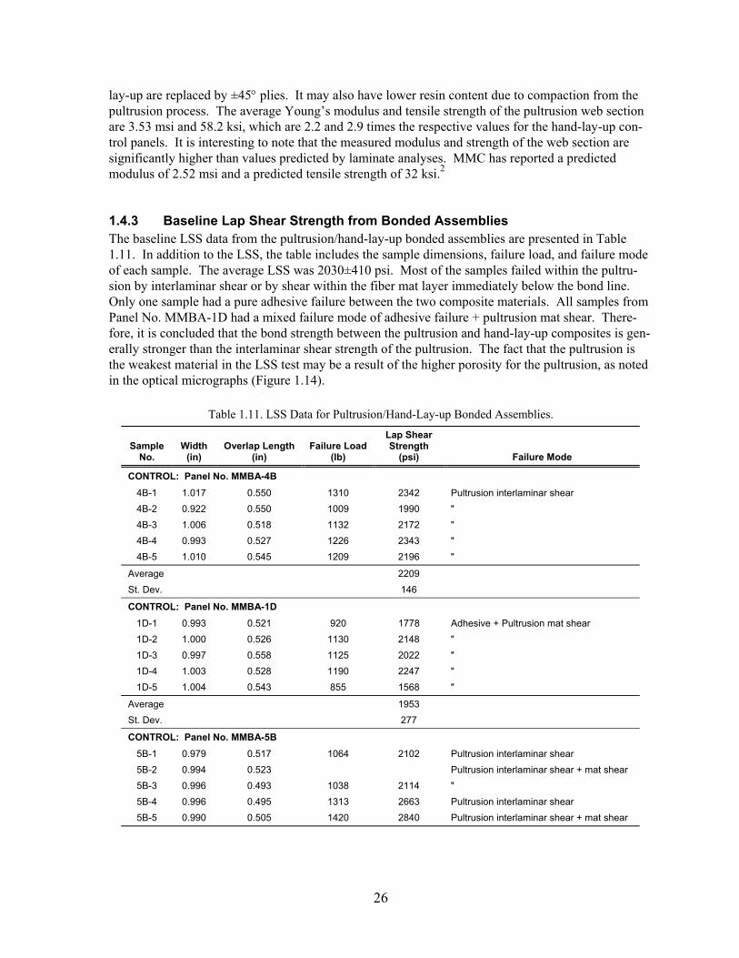
lay-up are replaced by ±45° plies. It may also have lower resin content due to compaction from the pultrusion process. The average Young’s modulus and tensile strength of the pultrusion web section are 3.53 msi and 58.2 ksi, which are 2.2 and 2.9 times the respective values for the hand-lay-up con-trol panels. It is interesting to note that the measured modulus and strength of the web section are significantly higher than values predicted by laminate analyses. MMC has reported a predicted modulus of 2.52 msi and a predicted tensile strength of 32 ksi.2

1.4.3 Baseline Lap Shear Strength from Bonded Assemblies The baseline LSS data from the pultrusion/hand-lay-up bonded assemblies are presented in Table 1.11. In addition to the LSS, the table includes the sample dimensions, failure load, and failure mode of each sample. The average LSS was 2030±410 psi. Most of the samples failed within the pultru-sion by interlaminar shear or by shear within the fiber mat layer immediately below the bond line. Only one sample had a pure adhesive failure between the two composite materials. All samples from Panel No. MMBA-1D had a mixed failure mode of adhesive failure + pultrusion mat shear. There-fore, it is concluded that the bond strength between the pultrusion and hand-lay-up composites is gen-erally stronger than the interlaminar shear strength of the pultrusion. The fact that the pultrusion is the weakest material in the LSS test may be a result of the higher porosity for the pultrusion, as noted in the optical micrographs (Figure 1.14).

Table 1.11. LSS Data for Pultrusion/Hand-Lay-up Bonded Assemblies.

Sample No.

Width (in)

Overlap Length (in)

Failure Load (lb)

Lap Shear Strength

(psi) Failure Mode

CONTROL: Panel No. MMBA-4B 4B-1 1.017 0.550 1310 2342 Pultrusion interlaminar shear 4B-2 0.922 0.550 1009 1990 " 4B-3 1.006 0.518 1132 2172 " 4B-4 0.993 0.527 1226 2343 " 4B-5 1.010 0.545 1209 2196 "

Average 2209 St. Dev. 146

CONTROL: Panel No. MMBA-1D 1D-1 0.993 0.521 920 1778 Adhesive + Pultrusion mat shear 1D-2 1.000 0.526 1130 2148 " 1D-3 0.997 0.558 1125 2022 " 1D-4 1.003 0.528 1190 2247 " 1D-5 1.004 0.543 855 1568 "


CONTROL: Panel No. MMBA-5B 5B-1 0.979 0.517 1064 2102 Pultrusion interlaminar shear 5B-2 0.994 0.523 Pultrusion interlaminar shear + mat shear 5B-3 0.996 0.493 1038 2114 " 5B-4 0.996 0.495 1313 2663 Pultrusion interlaminar shear 5B-5 0.990 0.505 1420 2840 Pultrusion interlaminar shear + mat shear

26

Sample No.

Width (in)

Overlap Length (in)

Failure Load (lb)

Lap Shear Strength

(psi) Failure Mode


CONTROL: Panel No. MMBA-3D 3D-1 0.991 0.489 810 1671 Adhesive 3D-2 1.000 0.510 979 Pultrusion interlaminar shear 3D-3 0.993 0.523 884 1702 Pultrusion mat shear 3D-4 0.989 0.541 759 1419 Pultrusion mat shear 3D-5 0.996 0.528 675 1284 Adhesive + Pultrusion mat shear


Average for All 4 Bonded Assemblies 2033 St. Dev. 407

1.4.4 Effects of Environmental Exposures on Mechanical and Physical Properties

1.4.4.1 E-glass/Epoxy Vinyl Ester Deck-Reinforcement Composite Panels The effects of the environmental exposures on the mechanical and physical properties of the E-glass/epoxy vinyl ester hand-lay-up system are summarized in Table 1.12. The table is a listing of the average tensile properties, glass-transition temperature, and hardness for the flat panels. Weight change data are given for the bonded assemblies as well as for the panels. The standard deviations for the average properties are also given. Detailed data for the individual tensile tests and hardness measurements are given in Appendix 2.

Moisture absorption is plotted as a function of exposure time for the 10,000-h panels and for the 12,910-h bonded assemblies in Figure 1.18. The curves show that the initial moisture absorption rates were higher for the panels than for the bonded assemblies, which were over twice the thickness of the panels. The relative rates for the different environments were consistent for the panels and bonded assemblies. In both cases, the highest rates were in the humidity chamber due to the higher temperature, and the lowest rates were in salt water. Initially, the curves followed normal Fick’s Law diffusion behavior with rapid initial moisture absorption followed by diminishing absorption rates as the equilibrium moisture content was approached. However, the moisture absorption rates subse-quently increased at exposure times between 167 and 333 days for the panels and between 333 and 417 days for the bonded assemblies. This type of behavior has been reported in the literature and was attributed to moisture saturation of the composite matrix followed by additional absorption within voids or other defects.17 The curves suggest that the panels may have reached the equilibrium moisture content at around 0.4−0.5%. Moisture content was still increasing at the end of the exposure periods for the thicker bonded assemblies. It is interesting to note that the bonded assemblies in the salt water and humidity exposures absorbed more moisture than the flat panels. This may indicate that the equilibrium moisture content for the Isophthalic polyester matrix of the pultrusion is higher than that for the epoxy vinyl ester matrix of the reinforcement panels. It may also be a consequence of the higher porosity within the pultrusion. Moisture can collect within voids, giving higher than normal moisture absorption.

27

Table 1.12. Mechanical and Physical Properties of E-glass/Epoxy Vinyl Ester after Environmental Exposures

Environmental Exposure

Young's Modulus

(msi)

Tensile Strength

(ksi) Failure Strain

(%) Matrix Tg (oC)

Hardness (Shore D)

Weight Change(Panels/BA)1

(%)

Control 1.60 + 0.08 20.3 + 1.4 1.77 + 0.14 87, 88, 88, 88 90 + 3

100% Humidity/38oC 1,000 h 1.60 + 0.09 21.4 + 0.6 1.85 + 0.10 95 88 + 2 0.20/0.18 3,000 h 1.68 + 0.13 17.8 + 0.7 1.56 + 0.11 103 88 + 1 0.31/0.29 10,000 h 1.46 + 0.06 16.1 + 0.3 1.37 + 0.07 102 89 + 2 0.40/0.55

Salt Water 1,000 h 1.48 + 0.04 19.1 + 0.7 1.80 + 0.16 90 89 + 1 0.13/0.20 3,000 h 1.76 + 0.14 18.6 + 0.9 1.63 + 0.17 98 90 + 2 0.21/0.33 10,000 h 1.50 + 0.10 21.6 + 1.3 1.95 + 0.12 88 87 + 2 0.36/0.58

pH 9.5 CaCO3 Solution 1,000 h 1.52 + 0.10 21.0 + 0.7 1.74 + 0.10 92 90 + 1 0.20/0.19 3,000 h 1.53 + 0.02 18.6 + 1.6 1.58 + 0.21 92 90 + 2 0.36/0.25 10,000 h 1.57 + 0.07 19.6 + 0.9 1.70 + 0.14 92 88 + 1 0.49/0.30

Dry Heat at 60oC 1,000 h 1.64 + 0.07 24.4 + 0.8 2.12 + 0.14 109 89 + 1 -0.09/-0.10 3,000 h 1.85 + 0.07 20.0 + 0.8 1.75 + 0.21 111 91 + 3 -0.09/-0.14

20 Freeze/Thaw Cycles 1.69 + 0.09 18.4 + 0.8 1.67 + 0.23 103 90 + 2 0.25

Diesel Fuel, 4 h 1.58 + 0.04 20.6 + 0.7 1.80 + 0.14 90 89 + 3 0

Weathering, ASTM G 53 1.66 + 0.06 20.9 + 1.0 1.74 + 0.06 102 92 + 1 -1.45 1 Weight change data for Bonded Assemblies (BA) are for 2,000, 5,000 and 12,910 h.

Young’s modulus following all exposure conditions was at least 90% of the average modulus for the control panels. Thus, it is concluded that the environmental exposures did not significantly degrade the modulus of the E-glass/epoxy vinyl ester composites. However, there may have been some deg-

0

0.1

0.2

0.3

0.4

0.5

0.6

0.7

0 100 200 300 400 500 600

Exposure Time, day

Moi

stur

e A

bsor

ptio

n, w

t%

Humidity, Panel Salt Water, Panel

Alkali, Panel Humidity, Assembly

Salt Water, Assembly Alkali, Assembly

Figure 1.18. Moisture absorption curves for fiberglass panels and bonded assemblies.

28

radation in moist environments. The 1,000- and 10,000-h salt water exposures had slightly lower than average modulus values, as did all three exposure periods in the pH 9.5 alkali solution. It is clear that any degradation that occurred in the alkali solution was not progressive since the modulus did not decrease with increasing exposure duration. Modulus reductions in the salt water and alkali expo-sures are believed to be due to plasticization of the epoxy vinyl ester matrix from moisture absorption. The modulus of the composite is somewhat sensitive to the matrix modulus due to the high fraction of off-axis (±45° and 90°) plies in the lay-up. Plasticization of the matrix also decreases the glass-transition temperature, and this issue will be discussed further below, along with a discussion of the Tg data.

The lowest average modulus measured for any exposure or control panel was 1.46 msi for the 10,000-h humidity exposure. In this case, the effect may have been progressive since no modulus reduction was observed for the 1,000- or 3,000-h exposures. Furthermore, the panels exposed to 3,000 and 10,000 h in the humidity chamber were the only panels to show significant reductions in tensile strength and failure strain. Tensile strength was reduced by 12% to 17.8 ksi after 3,000 h and by 21% to 16.1 ksi after 10,000 h. Similar reductions were measured for failure strain. These were statisti-cally meaningful reductions. The panels exposed to humidity for 3,000 and 10,000 h were the only exposure panels to have tensile strength and failure strain scatter bands (average strength ± standard deviation) that did not overlap with the scatter band for the four control panels. The strength reduc-tion for the humidity exposure is believed to be due to moisture attack of the E-glass fibers. The sus-ceptibility of E-glass fibers to strength reductions in moist environments is well documented.10,17 It is not surprising that strength reductions were measured for the humidity exposure, but not for the salt water and alkali exposures. It was demonstrated in the seismic retrofit of bridge columns durability test program that the humidity exposure at 38°C (100°F) is an accelerated test relative to the salt water and alkali exposures at 23°C (73°F).5 Similar results were measured for other E-glass/polyester and E-glass/vinyl ester composites in the seismic retrofit program.

The Tg data for the four control panels were very consistent, showing a variation of only 1°C (2°F) between 87 and 88°C (189 and 190°F). This indicates that the matrix is very stable at laboratory temperature since the first control panel was tested along with the 1,000-h exposure panels on July 9, 2002, while the last control panel was tested along with the 10,000-h exposures on August 6, 2003. The panels exposed to diesel fuel, salt water, or the alkali solution at 23°C (73°F) had no significant change in Tg. All of the exposures that involved elevated temperatures, the humidity chamber at 38°C (100°F), dry heat at 60°C (140°F), and the alternating humidity at 40°C (104°F), plus UV at 60°C (140°F) exposure caused increases in Tg. These results suggest that the epoxy vinyl ester resin was not fully cured at room temperature, and the elevated temperatures further advanced the cure state. This is further demonstrated by a comparison of the loss modulus versus temperature plots in Figure 1.19. The loss modulus curve for Control Sample No. 2 was nonsymmetrical with a peak at 88°C (190°F) and a shoulder at approximately 110°C (230°F). The curves for the samples exposed to the humidity chamber for 3,000 h and dry heat for 1,000 h are more symmetrical with narrow peaks that are shifted to higher temperatures. These curve changes are all indicative of cure advancement from the elevated temperature exposures.

A plot of Young’s modulus as a function of Tg is shown in Figure 1.20 for the E-glass/epoxy vinyl ester panels. The plot shows a general tendency for the composite modulus to increase as the cure state of the matrix advanced and Tg increased. The salt water and alkali solution exposures at 23°C

29

0

10

20

30

40

50

60

70

0 20 40 60 80 100 120 140 160 180 200

Temperature, oC

Loss

Mod

ulus

, ksi

Control C2

Dry Heat, 1000 h

Humidity, 3000 h

88oC 103oC

109oC

Figure 1.19. Loss modulus versus temperature for E-glass/epoxy vinyl ester control and exposure panels.

1.4

1.5

1.6

1.7

1.8

1.9

80 90 100 110 120

Glass Transition Temperature, oC

Youn

jg's

Mod

ulus

, msi

Control Panels

Moisture at 23CHumidity at 100F

Dry Heat at 60CHumidity at 38C/UV at 60C

Figure 1.20. Young’s modulus versus Tg for E-glass/epoxy vinyl

ester control and exposure panels.

(73°F) caused a decrease in modulus due to matrix plasticization even though there was either no change or just a slight increase in Tg. The panel exposed to salt water for 3,000 h deviated from this behavior in that it had a significantly higher modulus and Tg than the control panels. It is probable that this panel was inadvertently exposed to heat, probably sunlight, at some time. This most likely occurred during fabrication, shipping, or storage prior to the salt water exposure.

The panel exposed to the humidity chamber for 10,000 h was the only panel that deviated signifi-cantly from the correlation between Young’s modulus and Tg. This observation further supports the supposition that the E-glass fibers were attached by the 10,000-h humidity exposure. Thus, the modulus change for this panel was due to a different mechanism than that for the other panels.

It must be emphasized that the humidity exposure is an accelerated test and is much more severe than the environment at the King’s Stormwater Bridge location. High temperatures and low humidity during the summer will undoubtedly advance the cure state of the epoxy vinyl ester to a more stable

30

condition than the control panels. Little moisture absorption is expected due to the normally dry con-ditions and the thick layer of polymer concrete on the bridge deck surface. It should also be noted that the panel subjected to the weathering test showed no signs of modulus or strength degradation.

1.4.4.2 Pultrusion/Reinforcement Panel Bonded Assemblies The LSS data for the bonded assemblies subjected to the environmental exposures are tabulated in Table 1.13. The average LSS and standard deviation for the five tests for each exposure condition are given. The most frequent failure mode for the five tests for each exposure condition is also included in the table. A photograph showing examples of the different failure modes is shown in Figure 1.21. Detailed data for the individual LSS tests are given in Appendix 2.

Table 1.13. LSS Data for Bonded Assemblies After Environmental Exposures Environmental Exposure Lap Shear Strength (psi) Dominant Failure Mode

Control 2030 + 410 Pultrusion interlaminar shear 100% Humidity/38oC 2,000 h 1590 + 200 Pultrusion interlaminar shear + mat shear 5,000 h 2490 + 590 Pultrusion interlaminar shear 12,910 h 2270 + 150 Pultrusion interlaminar shear + mat shear Salt Water 2,000 h 2110 + 290 Adhesive + Pultrusion mat shear 5,000 h 2090 + 290 Pultrusion interlaminar shear + mat shear 12,910 h 2020 + 230 Pultrusion interlaminar shear + mat shear pH 9.5 CaCO3 Solution 2,000 h 2060 + 480 Adhesive + Pultrusion mat shear 5,000 h 2030 + 340 Pultrusion interlaminar shear + mat shear 12,910 h 2100 + 150 Pultrusion interlaminar shear Dry Heat at 60oC 2,000 h 2010 + 360 Adhesive + Pultrusion mat shear 5,000 h 1960 + 520 Pultrusion interlaminar shear 20 Freeze/Thaw Cycles 2280 + 170 Pultrusion interlaminar shear

Hand Lay-up Surface Pultrusion Surface

Adhesive + Hand Lay-up Mat Shear

Adhesive + Pultrusion Mat Shear

Hand Lay-up Interlaminar Shear

Pultrusion Interlaminar Shear

Pultrusion Mat Shear

2,000 h in Alkali Solution

Control

2,000 h at 140°F

12,910 h in Humidity at 100°F

12,910 h in Salt Water

Hand Lay-up Surface Pultrusion Surface

Adhesive + Hand Lay-up Mat Shear

Adhesive + Pultrusion Mat Shear

Hand Lay-up Interlaminar Shear

Pultrusion Interlaminar Shear

Pultrusion Mat Shear

2,000 h in Alkali Solution

Control

2,000 h at 140°F

12,910 h in Humidity at 100°F

12,910 h in Salt Water

Figure 1.21. Examples of failure modes exhibited by bonded assembly LSS samples.

31

The bonded assembly exposed to 100% humidity at 38° (100°F) for 2,000 h was the only exposure assembly with an average LSS that was less than 95% of the average LSS for the control assemblies. Although the average LSS for this exposure was 20% lower than the average LSS for the control assemblies, it was actually higher than the average LSS for one of the four control assemblies (see Table 1.11). Furthermore, the LSS was significantly higher following the 5,000-h and 12,910-h humidity exposures. Thus, it was concluded that the relatively low average LSS for the 2,000-h humidity exposure was probably due to variability between the bonded assemblies rather than any effects from the exposure environment. It was concluded that no significant degradation in LSS occurred for any of the environmental exposures.

Like the control bonded assemblies, most of the exposure bonded assemblies failed by interlaminar shear within the pultrusion. The bonded assemblies subjected to 2,000-h exposures to salt water, alkali solution, and dry heat all failed at the bond line and within the pultrusion mat layer. However, there was no reduction in LSS, and the samples subjected to longer exposures in these environments all failed within the pultrusion. Thus, there is no evidence that any of the exposures weakened the bond between the pultrusion and hand lay-up.

1.5 Summary and Conclusions The following conclusions were reached from environmental durability testing on AS4D-12K/EPON 826-EPICURE 9551 carbon/epoxy system used for girders on the King’s Stormwater Bridge.

TM

TM

1. The environmental exposures included in this test program did not cause any changes in physical appearance or microstructure to unidirectional panels or ring segments of the AS4D-12K/EPON 826-EPICURE 9551 system. TM

2. The average normalized tensile properties of unidirectional panels of the AS4D-12K/EPON 826-EPICURE 9551 system were: Young’s modulus = 13.1 ± 0.6 msi, ten-sile strength = 184 ± 26 ksi, and failure strain = 1.37 ± 0.17%. Tensile properties were not affected by any of the environmental exposures.

TM TM

3. Unidirectional panels of the AS4D-12K/EPON 826-EPICURE 9551 system absorbed 1−2 wt% moisture during exposure to 100% humidity at 38°C, salt water, or pH 9.5 alkali solution. The equilibrium moisture content was reached after approximately 80 days in each environment.

TM

4. The average epoxy matrix glass-transition temperature for unidirectional panels of the AS4D-12K/EPON 826-EPICURE 9551 system is 115 ± 2°C. T decreased to approximately 106°C following prolonged exposure to moisture in the humidity chamber, salt water, and alkali solution. T increased to approximately 121°C due to moisture dry-out during the dry heat exposure at 60°C and UV exposure of the weathering test. These small changes in T do not affect structural performance at bridge service temperatures.

TM TMg

TM

TM

gg

5. Ring segments from an AS4D-12K/EPON 826-EPICURETM 9551 girder absorbed 0.33−0.40 wt% moisture during exposure to 100% humidity at 38°C, salt water, or pH 9.5 alkali solution. The equilibrium moisture content was reached after approximately 170 days in each environment. The lower apparent equilibrium moisture content for the ring segments than for the unidirectional panels may be due to higher porosity in the panels.

TM

32

6. The average short-beam shear strength of ring segments of the AS4D-12K/EPONTM 826-EPICURETM 9551 is 4.0 ± 0.3 ksi. SBSS was not affected by any of the environmental exposures.

The following conclusions were reached from environmental durability testing on E-glass/DERAKANE 411-370 epoxy vinyl ester panels used to reinforce the bridge deck on the King’s Stormwater Bridge.

1. The environmental exposures included in this test program did not cause any changes in physical appearance or microstructure to panels or of the E-glass/DERAKANE 411-370 epoxy vinyl ester system.

2. The average tensile properties of the E-glass/DERAKANE 411-370 epoxy vinyl ester panels are: Young’s modulus = 1.60 ± 0.08 msi, tensile strength = 20.3 ± 1.4 ksi, and failure strain = 1.77 ± 0.14%. 100% humidity at 38°C was the only environmental exposure to have any significant effects on tensile properties. After 3,000 h in the humidity chamber, the tensile strength and failure strain were reduced by 12%. After 10,000 h, the tensile strength and fail-ure strain were reduced by 20%, and Young’s modulus was reduced by 10%.

3. E-glass/DERAKANE 411-370 epoxy vinyl ester panels absorbed 0.36−0.50 wt% moisture during 10,000-h exposures to 100% humidity at 38°C, salt water, or pH 9.5 alkali solution.

4. The average matrix glass-transition temperature for the as-processed E-glass/DERAKANE 411-370 epoxy vinyl ester panels was 88°C. Apparently, the panels were not fully cured at room temperature because Tg increased after exposure to the humidity chamber at 38°C, dry heat at 60°C, or to UV radiation at 60°C. Tg increased to 110°C for the 1,000- and 3,000-h dry heat exposures.

The following conclusions were reached from environmental durability testing on the bond between E-glass/DERAKANE 411-370 epoxy vinyl ester reinforcement panels and the E-glass/Aropol 7334T-15 Isophthalic polyester bridge deck used on the King’s Stormwater Bridge.

1. Optical microscopy demonstrated that a continuous bond was achieved between E-glass/DERAKANE 411-370 epoxy vinyl ester reinforcement panels and the E-glass/Aropol 7334T-15 Isophthalic polyester bridge deck material. The environmental exposures included in this test program did not cause any changes in physical appearance or microstructure of the bonded assemblies.

2. Bonded assemblies of the reinforcement panels with the pultruded bridge deck had an aver-age lap shear strength of 2030 ± 410 psi. The predominant failure mode was interlaminar shear within the E-glass/Aropol 7334T-15 Isophthalic polyester pultrusion. No significant degradation in LSS or change in failure mode occurred for any environmental exposure.

33

This page intentionally blank.

34

2. Durability of Composites Exposed to the Yolo Causeway Environment

2.1 Introduction In the late winter of 1997, Caltrans initiated a contract (#03379604) with Benco Contracting and Engineering to perform a seismic retrofit on the Interstate 80 Yolo Causeway. The retrofit consisted of constructing new concrete piles at every fourth bent, enclosing existing pile extensions with a composite case, and closing a longitudinal joint at the Tule Canal. The encasement of the concrete columns with composite materials was awarded to the Myers Technologies Business unit of C. C. Myers, Inc. and commenced in the summer of 1998, concluding in October, 1998.

The Yolo Causeway is the portion of I-80, just west of Sacramento that traverses an Estuary at the Tule Canal. It is just over 3 mi. long, a third of which is an earthen berm. The two bridges (22-0044W and 22-0045E) that constitute the remainder of the Causeway consist of six lanes of traffic (3EB & 3WB). The two outer lanes of the EB and WB original freeway are each supported with six 15-in.-dia columns (for a total of 12) that were retrofitted with composite cases. The newer inner lanes of the freeway are each supported with four octagonal columns, which were not encased. A total of more than 3,500 columns were retrofitted.

The composite encasement used to retrofit the pile extensions was a custom fiberglass fabric impreg-nated with a vinyl ester resin and pre-cured in the factory. The impregnated fabric was formed into cylindrical shells matching the column diameter. The shells were cured, slit lengthwise, and deliv-ered to the worksite. They were then bonded to the columns using an ambient-temperature cure, two-component adhesive. A height of 4 ft of each column was retrofitted using four concentric shells per column, with the slit offset on each successive layer.

The Yolo Causeway seismic retrofit project offered a unique opportunity to perform field studies to quantify the precise environment that composite casings see in service and to determine the durability of the composite materials in a field environment. During the winter months, all of the retrofit sec-tions are under water as the estuary is flooded. But in the summertime, the casings are subjected to hot, dry weather. Therefore, the Yolo Causeway represents one of the most severe environments that the composite casings will be subjected to in service in California.

In 1998, The Aerospace Corporation initiated an FHWA/Caltrans-sponsored project to perform a durability study on composite panels mounted on Yolo Causeway bridge columns, to monitor the local environment (temperature, humidity, and column pH) at the composite casing bond line, and to apply nondestructive testing techniques to detect bond line flaws and monitor flaw growth with time.19 The project was completed in 2001, but the durability study and environment monitoring were continued under the current Caltrans contract. Updated results are presented in this section and Section 3.

35

2.2 Materials and Field Exposure Procedures Flat panels of eight different composite systems supplied by six manufacturers are being exposed at the Yolo Causeway in a field study of environmental durability. The different systems and the num-ber of exposure panels for each system are given in Table 2.1. For most composite systems, the pan-els are from the same material lots that were used for laboratory durability testing conducted by The Aerospace Corporation as part of the Caltrans qualification program for composites for seismic retro-fit of bridge columns. Therefore, the material lots are well characterized, and the results of the field durability study can be compared with the results of the laboratory study. The effects of the environ-mental exposures are being determined from glass-transition temperature measurements, mass meas-urements, optical microscopy of cross sections, and tensile tests conducted in the fiber direction to determine Young’s modulus, ultimate tensile strength, and failure strain.

The test matrix also includes six bonded assemblies (MTA1-MTA6 in Table 2.1). Each bonded assembly consists of two 12 x 6 in. (30 x 15 cm) E-glass/Polyester panels bonded together with a polyurethane adhesive. These assemblies are being used for lap shear tests to determine the durability of the adhesive. Glass-transition temperature is also being measured for the adhesive.

Six separate panels are being exposed to the Yolo Causeway environment for six composite systems, and four panels are being exposed for the other three systems. The panels were mounted on octago-nal columns under the bridge. The general procedure was to attach all test panels for a given com-posite system to a single column. Furthermore, two panels were attached, one above the other, on one face of the octagonal column. Therefore, those systems with four test panels were placed on two faces of a column and those systems with six test panels were placed on three faces of a column. In most cases, the panels were placed on the south, southwest, and west faces of the column. This was done to protect the panels from impact damage from objects carried by wintertime water currents. The top of the upper panel was approximately 60 in. (150 cm) above ground level, and the top of the lower panel was approximately 47 in. (119 cm) above ground level.

In order to attach the panels to the columns, a 0.328 in-dia (0.833 cm-dia) hole was drilled through each panel on the centerline approximately 0.6 in. (1.5 cm) from each end. A polyethylene insert having an outside diameter of 0.312 in. (0.793 cm) and inside diameter of 0.260 in. (0.660 cm) was bonded in the hole. A polyurethane sealant was used to bond the inserts into the panels in order to

Table 2.1. List of Composite Materials for Yolo Causeway Field Durability Study Material Supplier System Type Composite System Panel Numbers

Master Builders Inc. Carbon/Epoxy CF130/MBrace Epoxy T3-2L13A & B, T3-2L24A & B, T3-2L25A & B

Mitsubishi Chemical Co. Carbon/Epoxy Replark 30/L700S-LS M2-2L13A & B, M2-2L21A & B, M2-2L22A & B

Xxsys Technologies, Inc. Carbon/Epoxy Akzo/Epon 828 X-P2C10A & B, X-P2C12A & B Fyfe Company Carbon/Epoxy SCH 41/Tyfo S HF-3I1 & 2, HF-3K1 & 2, HF-3M1 & 2 Fyfe Company E-glass/Epoxy SEH 51/Tyfo S HF-2I1 & 2, HF-2K1 & 2, HF-2M1 & 2 Fyfe Company Fiberglass/Epoxy SEH 51S/Tyfo S FG2I1 & 2, FG2J1 & 2 Hardcore Composites E-glass/Vinyl Ester E-glass/Vinyl Ester HD-P32A & B, HD-P34A & B Myers Technologies E-glass/Polyester E-glass/Polyester MT1 - MT6

Myers Technologies Adhesive Lap Shear Assemblies

E-glass/Polyester/ MOR-AD-695-28 Adhesive MTA1 - MTA6

36

seal the walls of the drilled holes to prevent water from wicking into the panels through exposed fiber ends. Two 0.156 in-dia (0.396 cm-dia) holes were drilled into the column for the attachment of each panel using 3/16 x 1.25 in. (0.476 x 3.18 cm) concrete screws. The composite panel inserts had a minimum length of 0.25 in. (0.64 cm). Therefore, the maximum penetration of the screws into the column did not exceed 1.0 in. (2.5 cm).

The panels were mounted on a total of nine columns to accommodate the full matrix of materials given in Table 2.1. There are three octagonal columns per bent. The octagonal columns are located in the middle of each bent between six circular columns on the north end and six circular columns on the south end. The circular columns, which support the original eastbound and westbound bridges, required seismic retrofit. The octagonal columns support the central expansion that was added between the original bridges and did not require seismic retrofit. The panels were mounted on all three octagonal columns on each of three bents, Bent Nos. 177, 178, and 179. For each bent, the octagonal columns were identified by their relative positions, north, center, or south.

The panels were mounted under the bridge on October 29, 1998. For those systems having six pan-els, one panel was removed for property measurements on September 5, 2000, and the second panel was to be removed in early spring 2001 as soon as the location was accessible after the water receded. The third and fourth panels were scheduled for removed in the fall of 2002 and spring of 2003, respectively. The fifth and sixth panels will be removed in the spring and fall, respectively, of 2008. The philosophy behind removing the panels for property measurements in the spring and fall is to make comparisons between panels with maximum moisture absorption (spring removal) and those that have dried-out over the hot, dry summer months. Panels are being removed in the spring and fall after approximately 2-, 4-, and 10-yr exposures. For those systems with four test panels, removal was planned for the spring and fall after 2 or 4 yr and after 10 yr.

The individual panels for each system are listed in Tables 2.2 and 2.3. The glass-fiber-reinforced systems are given in Table 2.2, while the carbon-fiber-reinforced systems are given in Table 2.3. The tables include the specific mounting location for each panel, the scheduled retrieval date, and the ini-tial mass. The actual retrieval date and final mass are given for those panels that have been retrieved. The planned retrieval dates are given by the month and year, while the actual retrieval dates are given by the month, day, and year.

Note that the panels originally scheduled for May 01 or May 03 retrieval were not retrieved. Unfor-tunately, the water level at the site during the 2000−2001 and 2002−2003 winter seasons was lower than normal so that the panels were not submerged. Therefore, the panels were not removed in the spring of 2001 or spring of 2003. The May 01 panels will be retrieved following the next winter having a water level sufficient to submerge the panels. New retrieval dates for the May 03 panels will be scheduled after the May 01 panels are retrieved and tested.

It should also be noted that mass was not monitored for the MT and MTA panels provided by Myers Technologies (Table 2.2). These panels were provided immediately before mounting. The inserts were bonded into the panels in the field. A balance was not available for initial mass measurements.

37

Table 2.2. Glass-Fiber-Reinforced Composite Panels Panel Location on Yolo Causeway Bridge Retrieval Initial Final

Number Bent No. Column Side Position Date Mass (g) Mass (g) HF-2I1 177 Center W Bottom May-08 323.36 HF-2I2 177 Center W Top Sep-08 325.24 HF-2K1 177 Center SW Top 11/14/02 332.11 332.02 HF-2K2 177 Center SW Bottom May-03 328.75 HF-2M1 177 Center S Top May-01 331.85 HF-2M2 177 Center S Bottom 9/5/2000 322.12 322.60 FG2I1 178 South W Top May-08 233.84 FG2I2 178 South W Bottom Sep-08 240.48 FG2J1 178 South S Top May-01 237.53 FG2J2 178 South S Bottom 9/5/2000 226.35 226.60 HD-P32A 179 North W Bottom May-08 233.96 HD-P32B 179 North W Top Sep-08 237.09 HD-P34A 179 North SW Top 11/14/02 233.59 233.25 HD-P34B 179 North SW Bottom May-03 237.61 MT1 179 Center S Bottom 9/5/2000 NA 202.80 MT2 179 Center S Top May-01 NA MT3 179 Center SW Bottom May-08 NA MT4 179 Center SW Top 11/14/02 NA NA MT5 179 Center W Bottom May-03 NA MT6 179 Center W Top Sep-08 NA MTA1 179 South S Bottom 9/5/2000 NA 422.50 MTA2 179 South S Top May-01 NA MTA3 179 South SW Bottom May-08 NA MTA4 179 South SW Top 11/14/02 NA NA MTA5 179 South W Bottom May-03 NA MTA6 179 South W Top Sep-08 NA

Table 2.3. Carbon-Fiber-Reinforced Composite Panels Panel Location on Yolo Causeway Bridge Retrieval Initial Final

Number Bent No. Column Side Position Date Mass (g) Mass (g) T3-2L13A 178 Center SW Top 11/14/02 76.87 76.63 T3-2L13B 178 Center SW Bottom May-03 78.48 T3-2L24A 178 Center S Top May-01 75.37 T3-2L24B 178 Center S Bottom 9/5/2000 74.72 74.90 T3-2L25A 178 Center W Top May-08 72.73 T3-2L25B 178 Center W Bottom Sep-08 68.83 M2-2L13A 177 North S Bottom 9/5/2000 89.65 89.3* M2-2L13B 177 North S Top May-01 84.20 M2-2L21A 177 North NW Top May-08 81.74 M2-2L21B 177 North W Top Sep-08 74.18 M2-2L22A 177 North SW Top 11/14/02 82.42 82.10 M2-2L22B 177 North W Bottom May-03 81.34 X-P2C10A 178 North W Top Sep-08 178.20 X-P2C10B 178 North W Bottom May-08 186.58 X-P2C12A 178 North SW Top May-01 191.54 X-P2C12B 178 North SW Bottom 9/5/2000 181.47 181.55 HF-3I1 177 South S Bottom 9/5/2000 155.49 155.70 HF-3I2 177 South S Top May-01 148.11 HF-3K1 177 South SW Top 11/14/02 155.36 154.95 HF-3K2 177 South SW Bottom May-03 153.56 HF-3M1 177 South W Top May-08 160.50 HF-3M2 177 South W Bottom Sep-08 163.69

*Insert pulled out

38

2.3 Testing Procedures The effects of the environmental exposures are being determined from matrix glass-transition tem-perature measurements, Tg, mass measurements, optical microscopy of cross sections, and tensile tests conducted in the fiber direction to determine Young’s modulus, ultimate tensile strength, and failure strain. Single-lap shear strength measurements are being made to determine any changes in the bond strength of the adhesive. Pre-exposure and post-exposure photographs are being taken to monitor changes in physical appearance.

Pre-exposure photographs were taken immediately after mounting the panels on the columns. Addi-tional field photographs were taken in September 1999 after one year of exposure and will be repeated periodically throughout the 10-yr exposure period. After the panels are removed from the columns and returned to the laboratory, they are being cleaned in tap water using a soft brush. After cleaning, additional photographs are taken to document any changes in physical appearance.

As noted above, a polyurethane sealant was used to bond the mounting inserts into the panels in order to seal the walls of the drilled holes to prevent water from wicking into the panels through exposed fiber ends. The sealant was also used to prevent wicking along any machined or saw-cut panels edges. Pre-exposure mass measurements were made after the polyurethane sealant cured at ambient temperature. Post-exposure mass measurements are being made after the panels are cleaned and dried.

Following mass measurements, the panels are being sectioned using a water-cooled diamond cut-off wheel to give a 10 x 6 in. (25 x 15 cm) area for the preparation of five tensile samples and a 0.5-in. (1.3 cm) wide strip for one Tg sample. The tensile and Tg samples are cut out with the sample length parallel to the primary fiber direction.

The sample preparation and testing procedures discussed in Subsection 1.2.4 for tensile testing and composite Tg measurements were used for the field durability study. Differential scanning calorime-try (DSC) using a TA Instruments Model No. 2910 DSC was used to measure Tg for the adhesive in the Myers Technologies, Inc. bonded assemblies. Approximately 5 mg of adhesive was scraped from the bond line of the bonded assemblies for analysis. Heat flow was measured during heating at 5°C/min (9°F/min) over the temperature of –60 to 100°C (–50 to 212°F). Tg was determined from plots of heat flow versus temperature following standard procedures.20

For the preparation of single-lap shear samples, the Myers Technologies, Inc. bonded assemblies are cut parallel to the fiber direction with the diamond cut-off wheel into five 6 x 1.0 in. (15 x 2.5 cm) strips. The two composite adherrends are cut along locations A and B as shown in Figure 1.4 (Subsec-tion 1.2.4) to form the lap shear area. Thus, the lap shear samples have a 0.5-in. (1.3-cm) long single-lap configuration. It is pointed out in ASTM D 4896,21 “Standard Guide for Use of Adhesive-Bonded Single Lap-Joint Specimen Test Results,” that the true shear stress of an adhesive joint can not be easily determined using single-lap specimens. The major problem is that the bending moment inher-ent in single-lap specimens induces tensile stresses normal to the plane of the bond line at the ends of the overlap and a nonuniform shear stress distribution in the adhesive. Thus, the measured shear stress at failure is lower than the true shear strength of the joint. This is not an issue for the thick composite adherrends used for MMC-bonded assemblies, but is for the thin composite adherrends in

39

the Myers Technologies, Inc. bonded assemblies. Therefore, the steel fixture shown in Figure 2.1 is used to reduce bending of the composite adherrends. The overlap area of the sample is centered within the 2-in. (5.1-cm) long fixture so that bending stresses on the adherrends are resisted by the steel plates at positions approximately 0.75 in. (1.9 cm) outside the overlap area. During installation, the screws are tightened only to the point at which the clamping force is sufficient to prevent the steel fixture from sliding down the sample under the force of gravity. Thus, high compressive normal stresses on the adhesive bond line are avoided. The fixture eliminates failures due to peeling stresses. The lap shear testing is performed in an Instron Universal Testing Machine at a crosshead rate of 0.1 in/min (0.25 cm/min).

2.4 Results and Discussion Comparative photographs taken immediately after mounting the panels on the columns in October 1998 and after the first year of exposure in September 1999 are shown in Figures 2.2 and 2.3 for one carbon-fiber-reinforced system and one glass-fiber-reinforced system. The effects of wintertime flooding and subsequent drying are evident by cracking of the soil around the columns in the one-year photographs. The panels were obviously soiled from the one-year exposure. Sample identification numbers were obscured or removed from several panels, particularly the E-glass/polyester panels fab-ricated by Myers Technologies, Inc. However, there was no evidence of physical damage to any of the composite panels following the first year of exposure. The photographs in Figures 2.2 and 2.3 are representative of composite systems fielded in the experiment. Photographs for all nine systems are documented elsewhere.19

The first set of panels was removed from the columns on September 5, 2000 after a 2-yr exposure to the Yolo Causeway environment. This set included one panel for all composite systems except the Hardcore Composites E-glass/vinyl ester system. The second set of panels was removed from the columns on November 14, 2002 after a 4-yr exposure. This set included one panel for all composite systems except the Fyfe Company SEH 51S/Tyfo S fiberglass/epoxy system and the Xxsys Tech-nologies, Inc. Akzo/Epon 828 carbon/epoxy system. The specific panels removed are identified in Tables 2.2 and 2.3. All of the remaining panels were inspected when the 2-yr and 4-yr panels were retrieved. None of the panels showed any evidence of physical damage.

Figure 2.1. Anti-bending fixture for single-lap shear testing.

40

Figure 2.2. Photographs of Fyfe Co. SCH 41/Tyfo S Carbon/Epoxy panels taken at

beginning (left) and after 1-yr field exposure

Figure 2.3. Photographs of Myers Technologies, Inc. E-glass/Polyester/MOR-AD-

695-28 Adhesive-bonded assemblies taken at beginning (left) and after 1-yr field exposure.

The retrieved panels were returned to the laboratory for cleaning, further inspection, and mechanical and physical property measurements. Visual inspection following brush cleaning in tap water gave no indications of any changes in physical appearance for any of the composite systems. Photographs (Figure 2.4) of the as-retrieved and cleaned 4-yr panels for the Mitsubishi Chemical Co. Replark

41

Inside Clean Outside Clean

Inside, As-Retrieved Outside, As-Retrieved

Inside Clean Outside CleanInside CleanInside Clean Outside CleanOutside Clean

Inside, As-Retrieved Outside, As-RetrievedInside, As-RetrievedInside, As-Retrieved Outside, As-RetrievedOutside, As-Retrieved

Figure 2.4. Photographs of Mitsubishi Chemical Co. carbon/epoxy

Panel No. M2-2L22A after 4-yr field exposure.

30/L700S-LS carbon/epoxy system are typical of all exposure panels. Considerable dirt and debris covered the outside and inside (against column) surfaces of the panels from submersion in the murky flood waters. However, cleaning restored the original appearance of all panels.

The tensile properties, matrix glass-transition temperature, and moisture absorption for the carbon-fiber-reinforced composites are given in Table 2.4. The data for the 2- and 4-yr Yolo Causeway exposure are compared to average values for four control (baseline) panels and the results of a 1.1-yr

Table 2.4. Mechanical and Physical Properties of Carbon-Fiber-Reinforced Composites

Composite System Exposure Conditions


Tensile Strength

(ksi

Failure Strain

(%) Matrix Tg

(oC)

Moisture Absorption

(%)

Fyfe Company SCH 41/Tyfo S Epoxy Control 9.15 + 0.27 136 + 9 1.44 + 0.11 68 2 yr at Yolo 9.78 + 0.39 144 + 7 1.48 + 0.12 68 0.14 4 yr at Yolo 9.35 + 0.39 138 + 7 1.43 + 0.10 70 -0.26 1.1 yr in Alkali Solution 9.50 + 0.28 144 + 6 1.45 + 0.06 64 1.28

Master Builders, Inc. CF130 (T700)/MBrace Epoxy Control 32.8 + 1.8 636 + 27 1.75 + 0.09 69 2 yr at Yolo 33.7 + 0.7 536 + 29 1.50 + 0.08 67 0.24 4 yr at Yolo 32.6 + 1.6 572 + 43 1.58 + 0.13 67 -0.31 1.1 yr in Alkali Solution 33.1 + 1.5 615 + 39 1.70 + 0.12 62 1.31

Mitsubishi Chemical Corp. Replark 30 (T700)/L700S-LS Epoxy Control 33.6 + 1.2 605 + 35 1.65 + 0.10 64 2 yr at Yolo 33.3 + 1.2 599 + 52 1.67 + 0.12 64 No Data 4 yr at Yolo 33.9 + 1.4 605 + 18 1.65 + 0.05 65 -0.39 1.1 yr in Alkali Solution 32.7 + 0.7 595 + 58 1.64 + 0.11 61 1.78 Xxsys Akzo/Epon 828 Epoxy Control 28.5 + 0.9 356 + 31 1.24 + 0.11 64 2 yr at Yolo 30.1 + 0.6 375 + 10 1.24 + 0.05 64 0.04 1.1 yr in Alkali Solution 26.3 + 0.6 381 + 11 1.42 + 0.04 52 0.96

42

(10,000-h) exposure to a pH 9.5 alkali solution. The control and alkali exposure data are from the laboratory qualification test program. The most severe exposures in the qualification program were 1.1 yr in 100% humidity at 38°C (100°F), 1.1 yr in salt water at room temperature, and 1.1 yr in the alkali solution at room temperature. None of these exposures had any significant effects on the ten-sile properties of any of the carbon/epoxy composite systems. However, the salt water and alkali exposures tended to have the most significant effect on Tg. Therefore, the alkali exposure was selected as being representative of the most severe exposures from the laboratory testing. The tensile properties shown in the table for the Yolo and alkali exposures are average values for five samples, while those for the control are average values for 20 samples. Standard deviations are also given. The Tg values are the averages for four samples from four different panels for the control condition and single samples for the Yolo and alkali exposures.

It is assumed that any changes in mass resulting from the exposure are due to moisture absorption or moisture dry-out. The 2-year panels all had small increases in mass, while the 4-year panels had small decreases. This is consistent with the fact that the panels were submerged in flood waters the first two winters, but were not submerged the third and fourth winters. Similar results were obtained for the glass-fiber-reinforced composites.

It should be noted that the tensile properties for the Master Builders, Inc., Mitsubishi Chemical Corp., and Xxsys Technologies, Inc. composites were calculated based on the know fiber area of the tensile samples. Therefore, the tensile properties are representative of the fiber properties in the fabricated composites. This is the standard method of calculating tensile properties used by Master Builders, Inc. and Mitsubishi Chemical Corp. Master Builders and Mitsubishi both use high-strength T700 carbon fibers. Therefore, it is not surprising that the Master Builders, Inc. CF130/MBraceTM epoxy and Mitsubishi Chemical Corp. Replark 30/L700S-LS systems had similar tensile properties. Xxsys Technologies, Inc. used a slightly lower modulus and significantly lower strength fiber; hence, the lower properties for their system. The tensile properties for the Fyfe Co. SCH 41/Tyfo S system are calculated using a standard thickness of 0.041 in./ply, which is similar to the actual per ply thickness of the composite. Thus, the SCH 41/Tyfo S properties are essentially based on the composite area and are, therefore, much lower than those for the other three carbon fiber systems, which were based on the fiber area only.

As the data in Table 2.4 demonstrate, the 1.1-year exposure in the alkali solution had no effects on the tensile properties of the carbon-fiber-reinforced systems. And as noted above, none of the laboratory exposures had a significant effect on the tensile properties of these systems. Therefore, no changes in tensile properties were anticipated from the 2-yr or 4-yr Yolo Causeway exposures. The anticipated results were obtained for the Fyfe Co., Mitsubishi Chemical Corp., and Xxsys Technologies, Inc. systems. However, the Master Builders, Inc. system had a 15% reduction in tensile strength and fail-ure strain relative to the control properties for the 2-yr panel and a 10% reduction in these properties for the 4-yr panel. We believe that this is an anomalous effect. The two-ply CF130/MBraceTM epoxy panels exposed at Yolo Causeway were 0.059 in. (0.150 cm) thick for the 2-yr exposure and 0.055 in. (0.140 cm) thick for the 4-yr exposure. The 18 panels tested in the laboratory environmental durabil-ity program were within the 0.038−0.048 in. (0.097−0.122 cm) thickness range. Optical micrographs presented in Figure 2.5 show that the higher thickness values for the Yolo panels were due to excess epoxy resin between the two layers of carbon fibers. This thick band of epoxy could affect load sharing between the two layers of fibers, thereby reducing tensile strength. In addition, the 2-yr and

43

Laboratory Control Panel

0.047 in.

2-yr Yolo Causeway Exposure Panel

0.060 in.

Closed Pores Planar Voids

Laboratory Control Panel

0.047 in.

2-yr Yolo Causeway Exposure Panel

0.060 in.

Closed Pores Planar Voids

Figure 2.5. Optical micrographs of Master Builders, Inc. laboratory control panel

and 2-yr Yolo Causeway exposure panel.

4-yr exposure panels had planar voids within epoxy-impregnated fiber plies, while the control panel had only closed pores. These large planar voids caused delaminations during tensile testing and probably reduced the tensile strength. Previous studies have shown that this system is susceptible to reduced tensile strength from delamination failures.22

The data in Table 2.4 show that the 2- and 4-yr Yolo Causeway exposures had no effects on Tg for the epoxy matrix of any of the four systems. The most frequent cause of reductions in Tg from envi-ronmental exposures is from moisture absorption, as demonstrated by the 1.1-year alkali exposure. In the present case, the Yolo Causeway panels were retrieved in the fall after being exposed to hot, dry weather throughout the summer. Thus, the moisture content was very low. In the future, panels will be removed in the spring immediately after the water level subsides. These panels should have the maximum absorbed moisture content, and thus the lowest Tg for the Yolo Causeway site.

The tensile properties, matrix glass-transition temperature, and moisture absorption for the glass-fiber-reinforced composites are given in Table 2.5. Glass fibers are susceptible to strength degrada-tion in moist environments, which was demonstrated in the laboratory durability testing. Strength degradation was particularly evident from the 100% humidity exposure at 38°C (100°F), especially for the SEH 51/Tyfo S and SEH 51S/Tyfo S systems. Therefore, the data in Table 2.5 includes 1.1-year data for the alkali solution and humidity exposures from the laboratory qualification test pro-gram for comparison with results for the 2- and 4-yr Yolo Causeway exposures.

The tensile properties for the SEH 51/Tyfo S and SEH 51S/Tyfo S systems are calculated using a standard thickness of 0.040 in./ply (0.102 cm/ply), which is similar to the actual per ply thickness of the composite. The tensile properties for the Myers Technologies, Inc. E-glass/Polyester system and Hardcore Composites E-glass/Vinyl Ester system are calculated using the actual sample area. Thus, the four glass-fiber-reinforced systems have similar tensile properties. The Fyfe Co. composites are reinforced by an unbalanced fabric, while the Hardcore Composites and Myers Technologies, Inc. systems are primarily reinforced by unidirectional fibers. As a result, the Fyfe Co. systems have lower Young’s moduli and higher failure strains than the Hardcore Composites and Myers Technolo-gies, Inc. composites.

44

Table 2.5. Mechanical and Physical Properties of Glass Fiber-Reinforced Composite Panels

Composite System Exposure Conditions

Young's Modulus

(msi)

Tensile Strength

(ksi) Failure

Strain (%) Matrix Tg

(oC)

Moisture Absorption

(%)

Fyfe Company SEH 51/Tyfo S

Control 3.96 + 0.13 80.5 + 5.1 2.10 + 0.18 66 2 yr at Yolo 4.13 + 0.14 79.9 + 2.8 2.03 + 0.03 68 0.15 4 yr at Yolo 4.00 + 0.11 80.1 + 1.8 2.06 + 0.07 68 -0.03 1.1 yr in Alkali Solution 3.88 + 0.06 62.4 + 2.5 1.63 + 0.08 64 0.88

1.1 yr in Humidity/38oC 3.93 + 0.18 51.4 + 2.1 1.31 + 0.08 73 1.09

Fyfe Company SEH 51S/Tyfo S

Control 5.03 + 0.12 111 + 3 2.56 + 0.13 74 2 yr at Yolo 5.15 + 0.06 110 + 1 2.45 + 0.08 72 0.11 1.1 yr in Alkali Solution 4.90 + 0.17 94 + 3 2.06 + 0.08 65 1.11

1.1 yr in Humidity/38oC 4.66 + 0.07 75 + 5 1.68 + 0.12 72 1.23

Myers Technologies, Inc. E-Glass/Polyester

Control 5.29 + 0.21 93 + 12 1.83 + 0.19 119 2 yr at Yolo 5.84 + 0.18 96 + 5 1.72 + 0.05 116 No Data 4 yr at Yolo 6.08 + 0.19 102 + 4 1.85 + 0.09 118 No Data 1.1 yr in Alkali Solution 5.20 + 0.11 82 + 4 1.67 + 0.10 88 0.30

1.1 yr in Humidity/38oC 5.45 + 0.23 86 + 7 1.61 + 0.08 113 0.20

Hardcore Composites E-Glass/Vinyl Ester

Control 5.30 + 0.35 108 + 13 2.19 + 0.30 113 4 yr at Yolo 5.18 + 0.44 126 + 14 2.51 + 0.11 110 -0.15 1.1 yr in Alkali Solution 5.20 + 0.21 90 + 6 1.78 + 0.20 109 0.40

1.1 yr in Humidity/38oC 4.85 + 0.31 93 + 12 1.98 + 0.18 109 0.16

The primary difference between the SEH 51/Tyfo S and SEH 51S/Tyfo S systems is the glass fibers. The SEH 51 fabric has E-glass fibers while the SEH 51S fabric has Owens Corning’s Advan-tex fiber. The Advantex fiber is a boron-free fiber developed by Owens Corning as a replacement for E-glass fibers. The mechanical properties of Advantex fibers are similar to those for E-glass fibers. In the present case, the SEH 51S/Tyfo S composite was 30% stronger than the SEH 51/Tyfo S composite. However, this is misleading since the SEH 51/Tyfo S composite tested in this program had lower tensile strength than typical SEH 51/Tyfo S composite lots.

The SEH 51/Tyfo S and SEH 51S/Tyfo S systems behaved similarly in the laboratory study. Nei-ther system was significantly affected by the 0.1- or 0.3-yr alkali solution exposures, but the tensile strength of both systems was degraded by over 15% following the 1.1-yr alkali exposure. In the humidity exposure at 38°C (100°F), both systems had a progressive decrease in tensile strength with exposure time. After 1.1 yr in the humidity chamber, the tensile strength of both systems was degraded by over 30%. The Myers Technologies, Inc. and Hardcore Composites systems were also degraded following the 1.1-yr exposures in the humidity chamber and alkali solution. However, the degradation was much smaller, around 10−15%.

45

The results for the 2- and 4-yr Yolo Causeway exposures were favorable since none of the four glass-fiber-reinforced systems showed any strength degradation. The total time that the 2-yr panels were submerged under water was determined from the output of humidity and temperature sensors applied to the columns (Section 3). The panels were submerged for approximately two months, from late February to late March, 1999 and 2000. During those periods, the column temperature was approxi-mately 50°F (10°C). Therefore, the total time under water at the Yolo Causeway (~0.15 yr) was less than the 0.3 yr laboratory exposure to the alkali solution. Furthermore, the temperature was much lower, which decreases the degradation rate. Therefore, the fact that none of the glass-fiber-reinforced systems showed any degradation after the 2-yr Yolo exposure is consistent with the labo-ratory results.

None of the glass-fiber-reinforced systems showed any significant changes in the matrix Tg after the 2- or 4-yr Yolo exposures. As for the carbon-fiber-reinforced systems, this observation is consistent with the fact that there was very little moisture absorption at the time that the panels were retrieved.

The lap shear strength and adhesive Tg results for the Myers Technologies, Inc. E-glass/polyester panels bonded together with MOR-AD-695-28 polyurethane adhesive are presented in Table 2.6. The dominant failure mode and relative porosity within the adhesive are also included in the table. The failure mode and relative porosity were determined by viewing the LSS fracture surfaces at a magni-fication of 10x with a stereo microscope. Myers Technologies, Inc. supplied seven bonded assem-blies for the Yolo Causeway field durability study. Six bonded assemblies were mounted on the col-umns, and one was maintained in The Aerospace Corporation Composites Laboratory as a control panel. The bonded assemblies were fabricated in September 1998 at the time that Myers Technolo-gies, Inc. was completing the Yolo Causeway seismic retrofit project. The bonded assemblies for the field durability study were fabricated following the same procedures that were used for preparing test panels for acceptance testing of the adhesive lots used in retrofit project. The Aerospace Corporation performed lap shear strength acceptance testing for six adhesive lots. The results from these tests are presented in the table along with the Yolo Causeway field durability study results to provide addi-tional baseline data.

Unfortunately, Myers Technologies, Inc. made a significant change in their fabrication process that invalidated the laboratory environmental durability test results. Initially, the E-glass/polyester com-posites were fabricated using a release film, which gave the composites a very smooth surface. Dur-ing environmental durability qualification testing, it was determined that the lap shear strength was only around 200 psi with the smooth composite surfaces. Myers Technologies, Inc. subsequently incorporated a woven peel ply into the composite fabrication process. The woven peel ply provides a very rough surface, which increased the lap shear strength to over 1000 psi. Shortly after incorporat-ing the woven peel ply into their process, Myers Technologies, Inc. provided two bonded assemblies to Aerospace for evaluation. One assembly, No. BP/10-1, was sectioned into four 6 x 4 in. (15 x 10 cm) sub-assemblies with one used for baseline testing and the other three placed into the humidity chamber on July 15, 1998. Part No. BP/10-1A was removed for testing after approximately 3,150 h (0.36 yr), and Part No. BP/10-1B was removed for testing along with the 2-yr Yolo Causeway panel. Part No. BP/10-1B was in the humidity chamber for 18,140 h (2.1 yr). Part No. BP/10-1C was left in the humidity chamber until November 2003, a 5.3-yr exposure period. Five lap shear samples 0.75 in. (1.9 cm) wide were tested for each subassembly. The data for this laboratory durability study are also included in Table 2.6.

46

Table 2.6. Lap Shear Strength of Polyurethane Adhesive Bonded Assemblies

Adhesive Assembly Set and Exposure Conditions

Lap Shear Strength

(psi) Failure Mode

Estimated Adhesive Porosity

Adhesive Tg (oC)

Yolo Causeway Field Durability Study 1 Control Assembly 2060 + 140 Adhesive Low 22 2 yr at Yolo 780 + 100 Cohesive High 22 4 yr at Yolo 830 + 60 Cohesive High 23

Yolo Causeway Seismic Retrofit Project Adhesive Acceptance Testing Assembly No. A8B16 1730 + 360 Mixed Mode High 25 Assembly No. A8B18 1510 + 140 Adhesive High Assembly No. A13B15 1370 + 90 Cohesive High Assembly No. A6B8 1690 + 180 Cohesive High Assembly No. A12B14 1200 + 140 Cohesive High Assembly No. A14B14 1730 + 130 Cohesive High

Limited Laboratory Durability Study 1 Control Assembly 1190 + 140 Adhesive Moderate 10

0.36 yr in Humidity/38°C 1460 + 50 Adhesive Moderate 13

2.1 yr in Humidity/38°C 900 + 40 Adhesive High 10

5.3 yr in Humidity/38°C 1060 + 160 Mixed Mode High

Expanded Laboratory Durability Study Assembly No. A13B15: 3 yr Lab. Exposure 1270 Mixed Mode High 21 Assembly No. A13B15: 3 yr Lab. Exposure + 0.11 yr (1000 hr) in Deionized Water

890 + 30 Mixed Mode High 23

Assembly No. A12B14: 5.8 yr Lab. Exposure 1420 + 270 Mixed Mode High Assembly No. A12B14: 3 yr Lab. Exposure + 2.8 yr (24,670 hr) in Deionized Water

1640 + 190 Adhesive Moderate

Yolo Durability Control Assembly: 0.28 yr (2500 hr) in Deionized Water

2150 + 170 Composite Shear + Adhesive

Low

Yolo Durability Control Assembly: 2.8 yr (24,670 hr) in Deionized Water

2200 + 200 Adhesive Low

The results for the field durability study show a 60% reduction in lap shear strength for the 2-yr and 4-yr exposures relative to the control assembly. Typical fracture surfaces shown in Figure 2.6 dem-onstrate that the control samples exhibited an adhesive failure mode with very low porosity, while the 2-yr and 4-yr exposure samples exhibited cohesive failures within the adhesive layer with high porosity. Tg of the MOR-AD-695-28 adhesive was 22 or 23°C (72 or 73°F) for the control and expo-sure assemblies. The results of the field durability study are inconclusive because it is impossible to determine whether the LSS reduction and changes in failure mode for the Yolo Causeway exposure samples are due to environmental effects or due to the high porosity in the adhesive layer.

The LSS data show a high degree of variability between the six Yolo Causeway seismic retrofit acceptance assemblies. Furthermore, some of these baseline assemblies failed predominantly in an adhesive mode, while others failed in a cohesive mode or a mixture of the two modes. All of the acceptance assemblies had relatively high porosity in the adhesive layer. It is interesting to note that the average LSS values of the acceptance panels were 330−860 psi lower than the average LSS for the Yolo Causeway control assembly, but were also 400−930 psi higher than the average LSS for the

47

Control: Adhesive Failure, Low Porosity

End

1: A

dhes

ive

End

2: B

are

Com

posi

te

2-yr Yolo Exposure: Cohesive Failure, High Porosity

End

2: P

orou

s Ad

hesi

ve

End

1: P

orou

s Ad

hesi

ve


End

1: A

dhes

ive

End

2: B

are

Com

posi

te


End

1: A

dhes

ive

End

2: B

are

Com

posi

te


End

2: P

orou

s Ad

hesi

ve

End

1: P

orou

s Ad

hesi

ve


End

2: P

orou

s Ad

hesi

ve

End

1: P

orou

s Ad

hesi

ve

Figure 2.6. Fracture surfaces of LSS samples from Myers Technologies, Inc. bonded assemblies.

2-yr and 4-yr exposure assemblies. Although these results clearly demonstrate that porosity dramati-cally reduces LSS, they also indicate that the Yolo Causeway environment may have caused addi-tional reductions in LSS. Thus, no definitive conclusion could be reached from these results.

The results for the laboratory humidity exposure were also inconclusive. In this case, the results were clouded by the fact that the glass-transition temperature of the adhesive in the bonded assembly (~10°C (~50°F)) was much lower than typical values of >21°C (70°F). Thus, the adhesive did not reach its normal cure state. This could be due to any of several causes, such as improper mixing, out-of-date material, or exposure to low temperatures during cure. Nevertheless, the LSS for the control samples (1190 ± 140 psi) was well above the minimum requirement of 800 psi for the Yolo Cause-way seismic retrofit project. After exposure to 100% humidity at 38°C (100°F) for 0.36 yr, the LSS increased by approximately 20%, and Tg increased from 10 to 13°C (50 to 55°F). These effects may be due to additional cure of the adhesive due to the elevated temperature in the humidity chamber. However, after exposure in the humidity chamber for 2.1 yr, the LSS decreased from 1460 to 900 psi (38% reduction), and Tg decreased back to 10°C (50°F). In addition, these samples had higher poros-ity, and the failure mode reverted from adhesive failures to cohesive failures. Finally, the samples exposed to the humidity chamber for 5.3 yr had an average LSS of 1060 ± 160 psi, which overlaps with the LSS scatterband for the control samples. Thus, the long-term humidity exposure, which is believed to be more severe for the adhesive than the Yolo Causeway environment, apparently did not degrade the adhesive LSS. However, the relevance of the data is uncertain due to the low initial Tg of the adhesive.

In view of these uncertainties, it was decided to perform additional laboratory durability studies using the Yolo Causeway control assemblies and remaining material from the Yolo Causeway adhesive acceptance testing assemblies. Shortly after testing the 2-yr Yolo Causeway samples, remaining material from acceptance assemblies A13B15 and A12B14 and a section from the Yolo Causeway control panel were submerged in a bath of deionized water at laboratory temperature. After 1,000 h (0.11 yr), three samples from Assembly No. A13B15 were tested along with one control sample. The LSS of the control sample was within the scatterband for the initial acceptance test data, but the LSS for the exposure samples was reduced by 35%. Adhesive porosity was high for all samples from Assembly No. A13B15, and there was no reduction in Tg from the water exposure. Three exposure samples from Assembly No. A12B14 were tested after 2.8 yr along with two control samples. In this case, one of the control samples and all three exposure samples had 25% higher LSS than the original acceptance data. However, they also had lower porosity. Finally, three samples from the Yolo Causeway durability study control assembly were tested after 2,500 hr (0.28 yr) in deionized water,

48

and four samples were tested after a 2.8-yr exposure. The LSS of all of these samples was within or greater than the scatterband for the control samples.

The contradictory results of these studies make it difficult to reach any conclusions regarding the durability of the adhesive bond. The water exposure data for the Yolo Causeway durability study control assembly suggests a high degree of moisture resistance for a high-quality bond with very low porosity in the adhesive layer. When porosity is present within the adhesive layer, which is usually the case for the Myers Technologies, Inc. process, the durability of the bond appears to be more unpredictable. It may well be that the durability depends upon the extent that moisture is able to penetrate the porous adhesive. Perhaps the most important observation is that the LSS of the 2-yr Yolo Causeway exposed assembly was slightly below the 800 psi requirement, and the LSS of the 4-yr exposure assemble was slightly above the requirement. It is important to continue the field dura-bility study on the remaining composite panels and bonded assemblies.

2.5 Summary and Conclusions The following conclusions were reached from 2- and 4-yr exposures to the Yolo Causeway environ-ment for four carbon-fiber-reinforced and four glass-fiber-reinforced composite systems.

1. Visual observations and comparisons of pre-exposure and post-exposure photographs gave no indications of any changes in physical appearance for any of the composite panels.

2. Pre-exposure and post-exposure mass measurements indicated that the moisture content of the composite panels did not vary significantly at the time of retrieval from the initial values.

3. Matrix glass-transition temperature for the exposed panels did not change significantly relative to baseline data for control samples.

4. There were no significant changes in Young’s modulus, tensile strength, or failure strain for any of the eight composite systems due to the Yolo Causeway exposure.

The following conclusions were reached from the Yolo Causeway field study and various laboratory studies on the environmental durability of the MOR-AD-695-28 polyurethane adhesive used to bond Myers Technologies, Inc. E-glass/polyester composite shells.

1. The glass-transition temperature of the MOR-AD-695-28 adhesive was not affected by 2- or 4-yr exposures to the Yolo Causeway environment or by a 0.11-yr immersion in deionized water.

2. The lap shear strength, failure mode, and environmental durability of Myers Technologies, Inc. bonded assemblies were greatly influenced by the degree of porosity within the MOR-AD-695-28 adhesive. When the porosity was low, the lap shear strength was >2,000 psi and the dominant failure mode was adhesive failure between the E-glass/polyester composite and adhesive layer. With low porosity, the lap shear strength was not degraded by a 2.8-yr immersion in deionized water. When the porosity was high, the lap shear strength was more

49

scattered (~800−1500 psi) and the failure mode was cohesive within the adhesive layer or a mixture of cohesive and adhesive failure modes. With high porosity, there were some indi-cations that the lap shear strength was susceptible to degradation due to water exposure.

3. Regardless of the porosity level and environmental exposure, the Myers Technologies, Inc. bonded assemblies generally had lap shear strengths ≥800 psi, the minimum LSS requirement for the Yolo Causeway seismic retrofit project. It is important to continue the filed durability study to ensure that the bonded assemblies continue to maintain the required LSS.

50

3. Environmental Monitoring of Composite Casings at the Yolo Causeway

3.1 Introduction and Background Adhesives need to perform for many years. Laboratories attempt accelerated tests to predict the use-ful lifetime of materials with tests performed in a reasonable time. The accelerated test methods involve exposing the materials to high temperatures and humidity. Mechanical tests are performed on these samples, and the results are compared to control samples that have been kept in a benign envi-ronment. To extrapolate the test results and predict the material’s lifetime, the conditions of the actual environment need to be determined. In addition, actual field condition monitoring verifies that the accelerated methodology was not benign or too severe.

The relative humidity (RH), temperature, and pH were measured underneath the composite, at the bond line between the adhesive and the concrete. The humidity and temperature were monitored hourly using a sensor and a data recorder that was downloaded every year. The pH was only meas-ured every one to two yr because it does not exhibit large day-to-day variations.

3.2 Temperature/Relative Humidity Sensors and Data Acquisition Onset Computer Corporation of Bourne, MA manufactured the sensors chosen to measure the tem-perature and relative humidity (HOBO Pro series). These battery-powered sensors can store up to 65,000 data points over a period of three years. The sensors were programmed to acquire temperature and humidity data every hour. They have the specifications listed in Table 3.1.

The response of the RH sensor used in these loggers varies not only with RH but also with tempera-ture. To display properly compensated RH values, the software takes the temperature data logged simultaneously with the uncompensated RH data and determines an RH adjustment factor. At 70°F, this adjustment factor is zero. At temperatures other than 70°F, the adjustment factor is added or sub-tracted to the uncompensated RH reading, dependent on whether the temperature is above or below 70°F. The result is the final compensated RH value.

Table 3.1. Specifications for Temperature/Humidity Sensors Specification Temperature Relative Humidity

Range -22 to 158°F 0 to 100% RH

Accuracy 0.7°F 3%

Resolution 0.5°F Drift 1% per yr Response Time <30 min <30 min in still air

Note: Relative Humidity is the ratio of the existing amount of water vapor in the air at a given temperature to the maximum amount that the air can hold at that temperature.

51

3.3 Sensor Mounting The sensors were mounted in sections of 3-1/2-in.-dia (8.89 cm-dia) PVC pipe (See Figure 3.1). The front of the sensor was in a small volume of air that would be exposed to the column concrete. The back of the sensor was mounted to a plate to make the data output port accessible by removing the watertight cover.

A PVC plug with a 1-in.-dia (2.5 cm-dia) hole in the center was bonded inside the end of the PVC pipe that mated with the composite casing. This end of the assembly was machined to a curvature that matched the curvature of the composite casing. During installation, a 1-in.-dia (2.5 cm-dia) hole was drilled in the composite overwrap using a core drill to expose the underlying concrete. The PVC pipe containing the sensor was bonded to the composite such that the sensor volume was directly over the hole in the composite. Miller Stephenson 907 ambient-temperature-curing epoxy adhesive was used to form a watertight bond between the PVC pipe and composite casing.

In this manner, the sensor measures the temperature and humidity of the air enclosed by the PVC pipe. This volume of air is directly exposed to the concrete. As the moisture in the concrete changes, the relative humidity in the enclosed volume of air changes correspondingly with a small time lag. The humidity and temperature data were taken each hour and stored in the sensor’s memory. The data were downloaded from the memory once every 1−2 yr by removing the back cover and con-necting a computer to the data output port. After the data were downloaded, the sensory memory was cleared and the sensor was programmed to continue acquiring data.

Seven temperature/humidity sensors were attached to the columns. As indicated in Table 3.2, six sensors were located on two adjacent bents, Bent Nos. 177 and 178, the same bents that were used for mounting the durability study panels. The round columns supporting the original freeway lanes were numbered 1−12 from south to north. Two sensors were mounted on each of two columns near the middle of the bridge (Bent 177 Column 7 and Bent 178 Column 8), while one sensor was mounted on each of two columns at the north (Bent 178 Column 12) and south (Bent 178 Column 3) sides of the bridge. All sensors on Bent Nos. 177 and 178 were mounted on the south side of the columns. The sensor mounted on Column No. 3 was exposed to direct wintertime sunlight, while the other columns

3.5 in. Dia. PVC PipeWith End Plugs

Adhesively Bonded toComposite Overwrap

Composite Overwrap1 in. Dia. Access Hole

Drilled Through Composite toExpose Sensor to Concrete

Concrete Column

Humidity and Temperature Sensor

Watertight Cover

Data Output Port3.5 in. Dia. PVC Pipe

With End PlugsAdhesively Bonded toComposite Overwrap

Composite Overwrap1 in. Dia. Access Hole

Drilled Through Composite toExpose Sensor to Concrete

Concrete Column

Humidity and Temperature Sensor

Watertight Cover

Data Output Port

Figure 3.1. Schematic diagram of sensor attachment to a composite overwrapped column.

52

Table 3.2. Bent and Column Locations for Temperature/Humidity Sensors Sensor Serial No. Bent No. Column No. Comments

230412 177 7 Near Casing Top 213671 177 7 Near Casing Middle 230411 178 8 Near Casing Top 213676 178 8 Near Casing Middle 213668 178 12 Near Casing Middle 213670 178 3 Near Casing Middle 213677 229 5 Near Casing Bottom, Large Debond

at Casing/Concrete Interface

were always shaded. None of the sensors saw direct sunlight in the summertime. For the columns that had two sensors, one sensor was located near the top of the composite casing and the other was located near the middle. These locations were selected to determine whether there was a gradient in temperature and humidity along the length of the casings. All other sensors were located near the middle of the casings. Finally, one sensor was located on a casing (Bent No. 229 Column No. 5) that had a large debond at the casing/concrete interface. The sensor was located directly over the debonded area. This sensor was located on the NW side of the column.

It was demonstrated in a previous study5 that the pH on the surface of concrete columns rapidly decreases from ≥14 to ≤9 as the concrete reacts with the environment. When the surface of the con-crete is sanded, as is done during the application of composite casings, fresh concrete with a higher pH is exposed. Once a composite casing is bonded to this surface, it is not known whether the casing protects the concrete from the atmosphere, maintaining a high pH, or if the pH diminishes with time like an unprotected concrete surface. Therefore, a number of columns were instrumented with pH cups for periodically measuring the concrete pH immediately under the composite casing.

The ph cups were standard Swagelock elbow fittings with a 1/4-in. (0.64-cm) pipe thread on one end and a female fitting for a 3/8-in.-dia (0.95 cm-dia) tube on the other end. A standard Swagelock cap was placed over the tube fitting. During installation, a 7/16-in.-dia (1.11 cm-dia) hole was drilled through the composite casing into the surface of the concrete column. The hole was threaded with a 1/4-in. pipe-thread (0.64-cm) tap for installation of the Swagelock fitting. The fitting was bonded to the threaded composite casing using Miller-Stephenson 907 epoxy adhesive. Measurements were made by removing the cap, filling the fitting and cavity with deionized water, and replacing the cap. Previous experience had shown that the water equilibrates with the concrete surface very rapidly so that accurate pH measurements can be made on the water within 1 hour. Initial pH measurements were made on October 29, 1998 using a battery-powered pH meter. However, it was determined that this degree of accuracy was not required and subsequent measurements on September 5, 2000 and November 4, 2002 were made using color-coded pH strips.

3.4 Results and Discussion The locations of the pH cups and results of the pH measurements are given in Table 3.3. A total of 12 pH cups were mounted on 10 different columns. The cups were located at a variety of bridge loca-tions (Bent Nos. 3 to 280 and Column Nos. 1 to 12) and were placed near the top, middle, and bottom of the composite jackets. Initial pH ranged from 6.9 to 9.8 with four measurements between 8.0 and

53

Table 3.3. Results of Concrete pH Measurements Under Composite Casings Bent No.

Column No.

Distance from Top of Casing (in.) Initial pH 10/29/98 pH 9/5/00 pH 11/14/02

3 11 1.5 8.3 7.5 7.0 51 5 4.0 8.6 7.5 7.0 51 5 1.8 7.8 7.0 7.0 71 4 17.5 8.9 111 11 16.0 9.3 8.0 7.0 177 6 5.0 9.6 7.5 7.0 180 4 14.0 9.8 7.5 7.0 182 7 11.0 9.7 8.0 7.5 202 12 3.0 9.4 9.0 7.0 234 1 9.5 6.9 7.5 7.0 280 4 7.0 9.8 7.5 7.0 280 4 21.0 8.0 7.5 7.0

8.9 and six between 9.0 and 9.8. These values were consistent with previous measurements on sanded, aged concrete.5 After 2 yr, the pH had decreased to 7−7.5 for 8 of the 12 cup locations, was 8 for two locations, and was 9 for one location. One cup could not be filled with water, indicating that a delamination had developed within the casing or between the casing and column. After 4 yr, the pH was 7 for 10 of the 11 remaining cups and 7.5 for the other cup. Thus, the pH of the concrete imme-diately under the composite casing had reached a neutral pH within 4 yr after installation of the casings.

Hourly data of the relative humidity and temperature at the bond line area of the Yolo columns were taken from October 27, 1998 to September 5, 2000. After downloading the data, an operating error was made when restarting the sensors, and no data were acquired from September 5, 2000 until November 14, 2002. On the latter date, the sensors were restarted, and data were taken until June 20, 2003. Thus, data were taken for a 2-yr period, followed by a 2-yr period in which no data were taken, and a final 7-month period in which additional data were taken. Data were successfully acquired on six of the seven sensors. No data were acquired from the sensor on Bent No. 229 Column No. 5, the column that had a delamination between the casing and column. Apparently, the delamination extended to the end of casing so that water was able to flow through the delamination into the PVC sensor cavity. Water flowed out of the sensor cavity when the watertight cover was removed. The sensor was no longer functional.

Plots of temperature and relative humidity as functions of time are shown in Figure 3.2 for the sensor located in the middle of the composite casing on Bent 178 Column 8. The temperature data show the anticipated daily night-to-day variations and were colder in the winter and warmer in the summer. In late winter/early spring, the area is flooded, and the composite casings and sensors are under water. This is evident in both the temperature and the humidity data because the day-to-night variation was much smaller during the period of flooding. The water stayed a relatively constant 51°F, especially in February of 2000 when the water level was higher than in 1999 or 2003.

The temperature rising and falling on a daily basis is expected. What requires further explanation is the concomitant rise and fall of the humidity measured by the sensors. As shown in Figure 3.1, the sensors are contained in a volume that is completely sealed, and (after an initial settling time) the only

54

0

20

40

60

80

100

Oct-98 Apr-99 Oct-99 Apr-00 Oct-00 Apr-01 Oct-01 Apr-02 Oct-02 Apr-03

Date

Tem

pera

ture

, o F

40

60

80

100

120

Rel

ativ

e H

umid

ity,

%

TemperatureRel. Humidity

Figure 3.2. Temperature and relative humidity for the casing middle on Bent 178 Column 8.

cause of humidity changes is from water vapor being absorbed or released by the concrete. It is not feasible that the amount of water contained in the concrete changes hourly, the apparent relative humidity changes must be due to another cause.

To answer this issue it is enlightening to look more closely at the humidity data. Temperature and humidity data taken over a five-day period in the summer of 1999 are shown in Figure 3.3. The graph shows both the absolute humidity in g/m3 and the relative humidity in %. It is apparent that the absolute humidity is in phase with the temperature, while the relative humidity is out of phase with the temperature. The relative humidity is falling when the temperature is rising. To make sure these data are consistent, all of the sensors were studied at different dates, and they all showed the same effect throughout the data acquisition period.

These results can be understood by considering how the temperature affects the moisture content in the gas in the sensor volume. If the volume was completely sealed and no moisture could come from

20

30

40

50

60

70

80

90

100

14-Jul-99 15-Jul-99 16-Jul-99 17-Jul-99 18-Jul-99 19-Jul-99Date

Tem

pera

ture

, o F

0

10

20

30

40

50

60

70

80

Hum

idit

y, g

/m3 o

r %

Temperature Rel. Humidity Absolute Humidity

Figure 3.3. Typical temperature and relative humidity data from the casing top

on Bent 177 Column 7 during five days in the summer of 1999. The labeled dates indicate midnight at the beginning of each day.

55

the concrete, then the absolute humidity, which is a direct measure of the moisture content, would be fixed. But the relative humidity, which is the ratio of the absolute humidity to the saturation moisture content at the air temperature, would still change with temperature. Since warm air holds more moisture than cold air, when the amount of moisture is fixed, the relative humidity decreases as the temperature increases.

For our case, the absolute humidity in the volume can change as water vapor flows between the con-crete column and the sensor volume. Let’s assume that the small surface area of the column in con-tact with the sensor volume is in thermal equilibrium with the gas and that the moisture content of the concrete surface remains in equilibrium with the adjacent concrete volume. Under these conditions, the absolute humidity in the sensor volume will increase with temperature because the equilibrium partial pressure of the fixed moisture content in the concrete increases with temperature. Qualita-tively, the measured data follows this behavior. However, this does not necessarily imply that the sensor volume is in equilibrium with the concrete. It simply means that the absolute humidity changes are consistent with an effort to maintain thermodynamic equilibrium. The sensor data are not sufficient to determine the extent to which equilibrium is approached.

Even though the absolute humidity in the sensor volume increased with temperature, the relative humidity decreased. This indicates that the magnitude of the moisture concentration increase for a given temperature change was less than the amount that the saturation concentration increases for that temperature change.

Data for the first two years from all six sensors were presented in Reference 19 and will not be repeated here. The plots in Figure 3.2 are representative of those for five of the six sensors for which data were obtained. The exception was the sensor located on Bent 178 Column 3, the column that was exposed to direct sunlight during the winter months. The sensor data for Bent 178 Column 3 are plotted in Figure 3.4 along with the data from Figure 3.2 for Bent 178 Column 8. The data clearly show higher daily peak temperatures for the Column 3 sensor due to direct sunlight from October to February for each of the three years. The direct sunlight also affected the relative humidity within the sensor volume. During periods of direct sunlight, the relatively humidity increased significantly for Column 3, but showed little change, aside from daily fluctuations, for the shaded Column 8. During

0

20

40

60

80

100

Oct-98 Apr-99 Oct-99 Apr-00 Oct-00 Apr-01 Oct-01 Apr-02 Oct-02 Apr-03Date

Tem

pera

ture

, o F

40

60

80

100

120

140

Rel

ativ

e H

umid

ity,

%

Temperature Column 3Temperature Column 8Rel. Humidity Column 3Rel. Humidity Column 8

Figure 3.4. Temperature and relative humidity data from the casing middle on

Bent 178 Column 3 and Column 8.

56

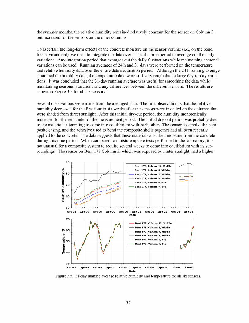
the summer months, the relative humidity remained relatively constant for the sensor on Column 3, but increased for the sensors on the other columns.

To ascertain the long-term effects of the concrete moisture on the sensor volume (i.e., on the bond line environment), we need to integrate the data over a specific time period to average out the daily variations. Any integration period that averages out the daily fluctuations while maintaining seasonal variations can be used. Running averages of 24 h and 31 days were performed on the temperature and relative humidity data over the entire data acquisition period. Although the 24 h running average smoothed the humidity data, the temperature data were still very rough due to large day-to-day varia-tions. It was concluded that the 31-day running average was useful for smoothing the data while maintaining seasonal variations and any differences between the different sensors. The results are shown in Figure 3.5 for all six sensors.

Several observations were made from the averaged data. The first observation is that the relative humidity decreased for the first four to six weeks after the sensors were installed on the columns that were shaded from direct sunlight. After this initial dry-out period, the humidity monotonically increased for the remainder of the measurement period. The initial dry-out period was probably due to the materials attempting to come into equilibrium with each other. The sensor assembly, the com-posite casing, and the adhesive used to bond the composite shells together had all been recently applied to the concrete. The data suggests that these materials absorbed moisture from the concrete during this time period. When compared to moisture uptake tests performed in the laboratory, it is not unusual for a composite system to require several weeks to come into equilibrium with its sur-roundings. The sensor on Bent 178 Column 3, which was exposed to winter sunlight, had a higher

50

60

70

80

90


Rel

ativ

e H

umid

ity,

%

Bent 178, Column 12, MiddleBent 178, Column 3, MiddleBent 177, Column 7, MiddleBent 178, Column 8, MiddleBent 178, Column 8, TopBent 177, Column 7, Top

.

35

45

55

65

75


Tem

pera

ture

, o F

Bent 178, Column 12, MiddleBent 178, Column 3, MiddleBent 177, Column 7, MiddleBent 178, Column 8, MiddleBent 178, Column 8, TopBent 177, Column 7, Top

Figure 3.5. 31-day running average relative humidity and temperature for all six sensors.

57

initial relative humidity and did not show the initial dry-out period. The higher daytime temperatures allowed more rapid moisture diffusion into the composite casing and adhesive on this column. Apparently, the composite and adhesive had already absorbed sufficient moisture to complete the dry-out period before the sensor was installed.

The averaged data accentuates the seasonal differences between the shaded columns and the sunlit column. The temperature data clearly shows a higher average temperature on the latter column from October to February of each year. During this period, the relative humidity increased more rapidly for this column than for the shaded columns. From April to October, the sensor on Column 3 showed no change in relative humidity, suggesting that equilibrium had been reached between the concrete and casing system. Meanwhile, the relative humidity continued to increase throughout the summer for the other columns.

It is interesting to note that the relative humidity showed little change for any of the sensors during the period of December 1999 through January 2000. All of the composite casings may have finally reached equilibrium with the concrete at that time. Then in early February 2000, the area was flooded, and another long period of moisture transfer from the concrete to the sensor volume was ini-tiated. The relative humidity continued to increase for the shaded columns until data acquisition was suspended on September 5, 2000. When the sensors were restarted on November 15, 2002, the aver-age relative humidity was approximately 5% higher than the September 2000 values, but showed no significant increase during the final data acquisition period. In fact, all six sensors indicated a small decrease in relative humidity during the final six weeks. It appears that equilibrium may have been reached for all four columns during the period between September 2000 and November 2002.

The average temperature data show remarkable consistency for the five sensors that were always shaded. Although there were clear differences in the absolute value of the relative humidity on these sensors, they displayed consistent seasonal humidity changes. The actual spread in the average rela-tive humidity among these sensors was typically around 6% at any given time. The reported accuracy of the relative humidity measurement is ±3%. Thus, within the measurement accuracy, the five sen-sors on the shaded columns had the same relative humidity at any given time. At the end of the sec-ond data acquisition period, when the sensor volumes appeared to be in equilibrium with the columns, the average relative humidity for the five sensors was 76 ± 2%.

The sensor on Bent 178 Column 3 had relative humidity values that were approximately 10% higher than the other sensors throughout the data acquisition periods. Although the different behavior of the data for this sensor with time can be explained by the fact that it was exposed to wintertime sunlight, it does not seem plausible that final, assumed equilibrium relative humidity should be any higher for this column than the shaded columns. Therefore, the final average relative humidity for this sensor, 88%, is considered questionable.

The sensor data has implications on the durability testing of composites for infrastructure applica-tions. Composite casings and adhesive bonds need to perform for many years. Laboratories attempt to predict the useful lifetime of materials using accelerated methods to perform tests in a reasonable time. The accelerated test methods involve exposing the materials to high temperatures and humidity, such as the 100% humidity at 100°F exposure specified in the Caltrans qualification program. To

58

extrapolate the test results and predict the material’s lifetime, the conditions of the actual environment need to be determined. In addition, actual field condition monitoring determines whether the acceler-ated methodology is either benign or too severe. This data shows that the current durability humidity tests are certainly not too severe. The composite material and the bondlines on the Yolo columns are being continuously subjected to 75% relative humidity at temperatures that frequently reach 90°F during the summer. The accelerated testing procedures need to be reviewed in light of this data.

3.5 Summary and Conclusions The following conclusions were reached from the pH, temperature, and humidity data taken at the concrete surface below the composite casings at the Yolo Causeway.

1. The pH of the concrete surface following surface preparation procedures, such as sanding, for the installation of composite casings was in the range between 8.0 and 10.0.

2. The pH of the concrete surface below the composite casing decreased to 7.5 to 8.0 one year after casing installation and to a neutral value of 7.0 two years after installation.

3. HOBO pro series temperature and humidity sensors manufactured by Onset Computer Corpo-ration were successfully used for monitoring the temperature and humidity at the concrete column/composite casing interface for a period up to three years at the Yolo Causeway.

4. A period in excess of two years after composite casing installation was required for the moisture content of the concrete column to reach equilibrium with the composite casing and adhesive system. The average relative humidity at apparent equilibrium was approximately 75%.

59


60

4. Long-Term Durability of E-glass/Polymer Composites

4.1 Introduction and Background Environmental durability testing was completed on three E-glass/polymer composite systems as part of the Caltrans Seismic Retrofit of Bridge Columns Program.5 The composite systems included the SEH 51/Tyfo S E-glass/epoxy system manufactured by Fyfe Co., the E-glass/polyester system manufactured by Myers Technologies, Inc., and the E-glass/vinyl ester system manufactured by Hardcore Composites. All three of theses systems demonstrated a susceptibility to moist environ-ments, which caused reductions in tensile strength. As discussed in Subsection 1.2.1, the moist envi-ronments include 100% humidity at 38°C (100°F) and immersion in salt water and pH 9.5 alkali solutions at 23°C (72°F). Property measurements were made after exposure times of 41.7, 125, and 417 days with the intent of using the data to make estimates of property degradation over the pro-jected service life. Unfortunately, in most cases, the E-glass-reinforced systems showed little evi-dence of degradation after the 41.7 and 125 day exposures, but had significant degradation following the 417 day exposure. Therefore, the data were insufficient for making long-term estimates of the tensile strength reductions. The issue was particularly important for the SEH 51/Tyfo S system because the strength reductions were much higher (up to 35%), and the strength was not recovered when the composite was allowed to dry-out. For the E-glass/polyester and E-glass/vinyl ester sys-tems, the strength reductions were <20%, and the strength was fully recovered when the composites were allowed to dry-out.

Two approaches were taken to address this issue. First, the composite panels subjected to the envi-ronmental exposures were intentionally cut-out significantly larger than the area of material required for post-exposure property measurements. Thus, excess materials were available to address any unanticipated issues. The excess materials for the three E-glass/polymer systems from the 417-day exposures were returned to the humidity chamber and salt water bath for longer term exposures. Ten-sile properties were measured after total exposure times of 2,363 days (6.47 yr).

The second approach was applied to the SEH 51/Tyfo S system. Several extra panels of the material lot used for durability testing remained in the laboratory. These panels were used to conduct addi-tional, accelerated durability testing. Four panels were immersed in deionized water at 70°C (158°F) for various times and the tensile strength was measured. The data from these exposures were com-bined with the 23°C (72°F) and 38°C (100°F) data from the original test matrix to develop a method-ology for predicting long-term strength reductions in moist environments as a function of exposure temperature.

4.2 Experimental Procedures The excess materials from the 417-day exposures were returned to the humidity chamber and salt water bath on July 20, 1998. They were removed for testing on November 17, 2003 for a total expo-sure period of 2,363 days. The materials were tabbed, cut into tensile samples, and tensile tested fol-

61

lowing the procedures given in Subsection 1.2.4. The pieces from the SEH 51/Tyfo S panels were 2.5 in. (6.4 cm) wide, which was sufficient to prepare four 0.5-in. (1.3-cm) wide tensile samples for each exposure condition. The pieces from the E-glass/polyester and E-glass/vinyl ester panels were at least 3.75 in. (9.5 cm) wide. Five 0.5-in. (1.3-cm) wide tensile samples were tested for each exposure condition for these composite systems.

For the accelerated durability testing, four SEH 51/Tyfo S panels, approximately 10 x 5 in. (25 x 13 cm) were prepared for the deionized water exposure. The panel edges were sealed with the same polyurethane adhesive that was used for the Yolo Causeway panels (Subsection 2.2). For these tests, the grip tabs were bonded onto to the panels before the exposures, rather than following the usual procedure of bonding the tabs after exposure. This allowed five tensile samples to be cut out from the panels and tested immediately after removal from the deionized water bath. The tensile samples were 0.75 in. (1.9 cm) wide.

The exposures were conducted by submerging the panels in deionized water in an aluminum baking pan approximately 14 in. long x 8 in. wide x 2 in. deep (36 x 20 x 5 cm) with an aluminum lid. The aluminum pan was placed on a hot plate to heat the deionized water to 70°C (158°F). The hot plate was plugged into a proportional controller with a control thermocouple sandwiched between the pan and hot plate. A second thermocouple was inserted into the water bath through a small hole in the aluminum lid. The setting of the controller was adjusted to maintain a water temperature of 70±2°C (158±4°F). The output of the thermocouple submerged in the water bath was monitored with a com-puter data acquisition system to ensure that the specified temperature was maintained. Water evapo-rated at a rate of approximately 400 ml/day (0.2 in. (0.5 cm) depth) and was replenished at least every 3rd day so that the panels were always completely submerged. The panels were removed from the water bath after 5.0 days (Panel No. 1K2), 17.0 days (Panel No. 1O2), 34.9 days (Panel No. 1K1), and 187 days (Panel No. 1O1).

4.3 Results and Discussion The tensile properties of the SEH 51/Tyfo S, E-glass/vinyl ester, and E-glass/polyester composites following the 2,363-day exposures in the humidity chamber and salt water bath are presented in Tables 4.1−4.3. The tables also include data for the control samples and 41.7-, 125-, and 417-day exposures from qualification testing.5 Semi-logarithmic plots of tensile strength versus Log exposure time are presented in Figures 4.1−4.3. For these plots, the tensile strength was normalized relative to the average tensile strength of the control samples.

The average Young’s modulus for all three composite systems following the 2,363-day exposures was essentially equal to the average modulus of the control samples. These results are consistent with those obtained for the shorter exposure periods. Therefore, the current results verify the conclusion from the qualification program that Young’s modulus for these composite systems is not affected by long-term exposures to moist environments.

Figure 4.1 shows that the tensile strength versus Log exposure time plots were linear for the salt water and humidity exposures for the SEH 51/Tyfo S system. The 100% humidity at 38°C (100°F) expo-sure caused significant strength reductions after only 41.7 days, while the salt water and alkali expo-sures at 23°C (72°F) did not cause any reduction until >125 days. However, once the degradation

62

Table 4.1. Tensile Properties of SEH 51/Tyfo S after 2,363-day Exposures Exposure Condition

or Sample No. Young's Modulus

(msi) Tensile Strength


(%)

2,363 days in 100% Humidity at 38oC HF-1E9 4.07 35.6 0.90 HF-1E10 4.22 40.5 0.98 HF-1E11 3.60 43.6 1.22 HF-1E12 3.94 43.2 1.10

Average 3.96 40.7 1.05 St. Dev. 0.26 3.7 0.14

2,363 days in Salt Water at 38oC HF-1H6 3.85 39.5 1.02 HF-1H7 3.97 45.6 1.17 HF-1H8 3.86 45.2 1.18 HF-1H9 4.10 45.9 1.12

Average 3.95 44.1 1.12 St. Dev. 0.12 3.0 0.07

Average Data from Durability Test Program Control 3.96 + 0.13 80.5 + 5.1 2.10 + 0.18 Humidity, 41.7 days 4.04 + 0.13 71.6 + 2.8 1.82 + 0.08 Humidity, 125 days 3.94 + 0.10 67.9 + 1.9 1.77 + 0.05 Humidity, 417 days 3.93 + 0.18 51.4 + 2.1 1.31 + 0.08 Salt Water, 41.7 days 4.03 + 0.09 80.8 + 2.2 2.07 + 0.06 Salt Water, 125 days 4.02 + 0.04 81.7 + 1.2 2.09 + 0.03 Salt Water, 417 days 4.09 + 0.07 66.0 + 1.9 1.64 + 0.04

0.0

0.1

0.2

0.3

0.4

0.5

0.6

0.7

0.8

0.9

1.0

1 10 100 1000 10000 100000

Exposure Time, day

Nor

mal

ized

Ten

sile

Str

engt

h HumiditySalt WaterAlkaliHumidity Curve FitSalt Water Curve Fit

Figure 4.1. Retained tensile strength versus Log of exposure time in 100% humidity or salt

water for SEH 51/Tyfo S.

63

Table 4.2. Tensile Properties of E-glass/Vinyl Ester after 2,363-day Exposures Exposure Condition




(%)

2,363 days in 100% Humidity at 38oC HD-P10I 5.21 75.4 1.40 HD-P10J 4.99 80.1 1.62 HD-P10K 4.56 76.8 1.67 HD-P10L 6.01 97.6 1.70 HD-P10M 5.51 93.4 1.27

Average 5.26 84.7 1.53 St. Dev. 0.55 10.2 0.19

2,363 days in Salt Water at 38oC HD-P11I 5.42 84.1 1.57 HD-P11J 6.31 89.1 1.42 HD-P11K 6.16 104.0 1.71 HD-P11L 4.34 73.9 1.66 HD-P11M 4.19 67.9 1.60

Average 5.28 83.8 1.59 St. Dev. 0.99 14.0 0.11

Average Data from Durability Test Program Control 5.30 + 0.35 108 + 13 2.19 + 0.30 Humidity, 41.7 days 5.02 + 0.13 106 + 10 2.20 + 0.19 Humidity, 125 days 5.07 + 0.12 106 + 4 2.21 + 0.16 Humidity, 417 days 4.85 + 0.31 93 + 12 1.98 + 0.18 Salt Water, 41.7 days 4.94 + 0.35 107 + 8 2.30 + 0.13 Salt Water, 125 days 4.90 + 0.14 104 + 6 2.26 + 0.14 Salt Water, 417 days 4.94 + 0.22 87 + 7 1.86 + 0.17

0.0

0.1

0.2

0.3

0.4

0.5

0.6

0.7

0.8

0.9

1.0

1 10 100 1000 10000 100000

Exposure Time, day

Nor

mal

ized

Ten

sile

Str

engt

h

HumiditySalt WaterAlkaliHumidity Curve FitSalt Water Curve Fit


water for E-glass/vinyl ester.

64

Table 4.3. Tensile Properties of E-glass/Polyester after 2,363-day Exposures Exposure Condition




(%)

2,363 days in 100% Humidity at 38oC FP16C6 5.41 86.0 1.61 FP16C7 5.05 76.6 1.51 FP16C8 5.21 65.5 1.30 FP16C9 5.08 78.1 1.54 FP16C10 4.98 76.7 1.54

Average 5.15 76.6 1.50 St. Dev. 0.17 7.3 0.12

2,363 days in Salt Water at 38oC FP39D6 5.19 85.9 1.68 FP39D7 5.08 87.0 1.70 FP39D8 5.14 81.7 1.60 FP39D9 5.27 83.3 1.64 FP39D10 5.17 91.4 1.77

Average 5.17 85.9 1.68 St. Dev. 0.07 3.7 0.06

Average Data from Durability Test Program Control 5.29 + 0.21 93 + 12 1.83 + 0.19 Humidity, 41.7 days 5.65 + 0.28 92 + 9 1.75 + 0.18 Humidity, 125 days 5.54 + 0.09 101 + 2 1.96 + 0.08 Humidity, 417 days 5.45 + 0.23 86 + 7 1.61 + 0.08 Salt Water, 41.7 days 5.75 + 0.21 106 + 3 1.98 + 0.08 Salt Water, 125 days 5.69 + 0.16 98 + 3 1.83 + 0.07 Salt Water, 417 days 5.29 + 0.14 93 + 1 1.82 + 0.05

0.0

0.1

0.2

0.3

0.4

0.5

0.6

0.7

0.8

0.9

1.0

1 10 100 1000 10000 100000

Exposure Time, day

Nor

mal

ized

Ten

sile

Str

engt

h

Humidity

Salt Water

Alkali

Humidity Curve Fit

Salt Water Curve Fit


water for E-glass/polyester.

65

initiated in salt water, it proceeded rapidly so that the strength reduction was approximately 50% of the control strength following the 2,363-day exposure in either the humidity chamber or salt water.

Vinyl ester and polyester matrices absorb much less water than the Tyfo S epoxy matrix, which greatly enhances the resistance of E-glass/vinyl ester and E-glass/polyester composites to strength reductions in moist environments. Neither of these systems had strength reductions >10% for expo-sure times <417 days. Furthermore, strength reductions in the 100% humidity at 38°C (100°F) envi-ronment were no greater than those in the salt water or alkali solutions at 23°C (72°F). The retained strength was >75% for both of these systems after 2,363 days in either environment. It should be noted that for the E-glass/polyester system the average tensile strength after 125 days in the humidity chamber and after 41.7 days in the salt water bath were over 10% higher than the average for the control samples. For this system, the tensile strength was normalized to these higher strength values for the plots in Figure 4.3.

Least-squares analyses of the humidity and salt water exposure data were performed to generate the curve fit lines included in Figures 4.1−4.3. Least-squares curve fit parameters for the equation NTS = A + B{Log(t)}, where NTS is the normalized tensile strength, t is the exposure time in days, and A and B are the curve fit parameters, can be used to make long-term strength predictions. The curve fit parameters are presented in Table 4.4 along with normalized strength predictions for 30-yr and 50-yr service lives. For the SEH 51/Tyfo S system the retained strength is 30−35% of the original strength after 30 yr and 20−30% after 50 yr. The slope of the curves is much lower for the E-glass/vinyl ester and E-glass/polyester composites so that these systems have predicted strengths after 50 yr that are similar to those after 30 yr. After 30 or 50 yr, the retained strength is approximately 65% of the original strength for the E-glass/vinyl ester system and approximately 70% for the E-glass/polyester system.

The results of the tensile strength measurements following the exposures in deionized water at 70°C (158°F) for the SEH 51/Tyfo S system are presented in Table 4.5. As expected, the degradation was more rapid at 70°C (158°F) than at the lower temperatures. The tensile strength was reduced by 22% after only 17 days and 49% after 35 days at 70°C (158°F) versus 11% after 41.7 days in 100% humidity at 38°C (100°F). No differences in physical appearance or failure mode were observed fol-lowing the 70°C (158°F) exposure in deionized water as compared to the humidity, salt water, and alkali solution exposures. Therefore, it was concluded that the 70°C (158°F) exposure in deionized water was a valid accelerated test.

Table 4.4. Curve Fit Parameters for Long Term Tensile Strength Predictions Composite System

Environment Intercept,

A Slope,

B Time Range

(day) NTS at 30 yr NTS at 50 yr

Fyfe Co. SEH 51/Tyfo S 100% Humidity at 38oC 1.29 -0.236 >42 0.34 0.28 Salt Water at 23oC 1.78 -0.366 >125 0.30 0.22

Hardcore Composites E-Glass/Vinyl Ester 100% Humidity at 38oC 1.29 -0.152 >125 0.68 0.64 Salt Water at 23oC 1.23 -0.140 >125 0.66 0.63

Myers Technologies, Inc. E-Glass/Polyester 100% Humidity at 38oC 1.15 -0.109 >42 0.71 0.69 Salt Water at 23oC 1.16 -0.105 >42 0.74 0.71

66

Table 4.5. SEH 51/Tyfo S Tensile Strength Following Deionized Water Exposure at 70°C

Sample No. Exposure Time

(Day) Tensile Strength

(ksi) NTS

HF-1K2A 5.0 70.3 HF-1K2B 5.0 74.8 HF-1K2C 5.0 79.9 HF-1K2D 5.0 74.4 HF-1K2E 5.0 77.3 HF-1O2A 17.0 62.6 HF-102B 17.0 62.8 HF-1O2C 17.0 65.4 HF-1O2D 17.0 61.3 HF-1O2E 17.0 61.4 HF-1K1A 34.9 41.4 HF-1K1B 34.9 40.4 HF-1K1C 34.9 40.4 HF-1K1D 34.9 40.9 HF-1K1E 34.9 41.5 HF-1O1A 187.0 37.5 HF-101B 187.0 39.9 HF-1O1C 187.0 41.6 HF-1O1D 187.0 42.5 HF-1O1E 187.0 40.6 Average for 5.0 days 75.3 0.94 Average for 17.0 days 62.7 0.78 Average for 34.9 days 40.9 0.51 Average for 187 days 40.4 0.50 Control Average 80.5 1.00

The accelerated data were combined with the data from the qualification testing for the humidity, salt water, and alkali solution exposures to develop Arrhenius expressions for relating residual strength to exposure time and temperature in moist environments. Analysis procedures published by Litherland, et al.10 were followed. The first step in the analysis was to make Log-Log plots of the normalized tensile strength versus exposure time for each exposure temperature, i.e., 23°C (72°F) for salt water and alkali solutions, 38°C (100°F) for the humidity chamber, and 70°C (158°F) for deionized water. These plots are shown in Figure 4.4. The next step was to perform least-squares analyses of the data at each temperature as shown in the figure. These expressions were used to calculate the exposure time required to degrade the strength to several specific levels, NTS = 0.85, 0.70, 0.55, 0.40, 0.32, and 0.25, at each of the three temperatures. Log exposure time was then plotted as a function of 1/T for each strength level in Figure 4.5, where T is the absolute temperature. Finally, a least-squares analysis was performed on the calculated data points in Figure 4.5 to establish a relationship between Log exposure time and 1/T for each NTS level. The six linear curves in Figure 4.5 can be used to estimate the remaining tensile strength at the end of life for a given service temperature in a moist environment.

67

0.1

1.0

1 10 100 1000 10000

Exposure Time, day

Nor

mal

ized

Ten

sile

Str

engt

h

38C Data23C Data70C Data40C Curve Fit23C Curve Fit70C Curve Fit

Figure 4.4. Retained tensile strength as a function of exposure time at 23, 38, and 70°C

for SEH 51/Tyfo S.

1

10

100

1000

10000

100000

1000000

0.0028 0.0030 0.0032 0.0034 0.0036

(Temperature)-1, K-1

Expo

sure

Tim

e, d

ay

NTS = 0.85 = 68.4 ksi NTS = 0.70 = 56.4 ksi NTS = 0.55 = 44.3 ksiNTS = 0.40 = 32.2 ksi NTS = 0.32 = 25.8 ksi NTS = 0.25 = 20.1 ksi0.85 Curve Fit 0.70 Curve Fit 0.55 Curve Fit0.40 Curve Fit 0.32 Curve Fit 0.25 Curve Fit

50 yr Service Life

Figure 4.5. Predicted retained tensile strength as a function of exposure time and temperature

for SEH 51/Tyfo S.

A line was drawn across Figure 4.5 at a service life of 50 yr. The estimated tensile strength after 50 yr is approximately 40% of the initial strength at 23°C (72°F) and approximately 32% at 38°C (100°F). These values are higher, particularly at 23°C (72°F), than the respective values of 22% and 28% calculated using the more simplistic approach presented in Figure 4.1. The curves in Figure 4.5 probably give better estimates because of the more rigorous approach, which better utilizes all of the available data.

68

4.4 Summary and Conclusions The following conclusions were reached from long term durability testing of Fyfe Co. SEH 51/Tyfo S, Hardcore Composites E-glass/vinyl ester, and Myers Technologies, Inc. E-glass/polyester compos-ites in moist environments.

1. Young’s modulus was not affected for any of the E-glass/polymer composites by 2,363-day exposures to 100% humidity at 38°C (100°F) or salt water at 23°C (72°F).

2. The tensile strength of the SEH 51/Tyfo S system was reduced by approximately 50% after 2,363 days in either 100% humidity at 38°C (100°F) or salt water at 23°C (72°F).

3. The tensile strength of the E-glass/vinyl ester and E-glass/polyester composite systems was reduced by <25% after 2,363 days in 100% humidity at 38°C (100°F) or salt water at 23°C (72°F).

4. Plots of normalized tensile strength versus Log exposure time followed a linear relationship for the three E-glass/polymer systems and can be used to make tensile strength predictions for long-term service.

The following conclusions were reached for accelerated durability testing of Fyfe Co. SEH 51/Tyfo S in deionized water at 70°C (158°F) and the use of accelerated data for making long-term strength predictions in moist environments.

1. No changes in tensile test failure mode or physical appearance occurred for SEH 51/Tyfo S exposed to deionized water at 70°C (158°F) versus exposures to 100% humidity at 38°C (100°F) or salt water at 23°C (72°F). It was therefore concluded that exposure to deionized water at 70°C (158°F) is a valid accelerated test.

2. Arrhenius plots can be used to combine durability data from exposures in deionized water at 70°C (158°F), 100% humidity at 38°C (100°F), and alkali or salt water at 23°C (72°F) to make long-term strength predictions for SEH 51/Tyfo S.

3. Projected tensile strength for SEH 51/Tyfo S after 50-yr exposure to moist environments is ~40% of the initial strength for exposure at 23°C (72°F) and ~32% of the initial strength for exposure at 38°C (100°F).

69

References

1. F. Seible, V. M. Karbhari, G. Hegemier, R. Burgueno, A. Davol, and L. Zhao, “Carbon/Epoxy Shell Fabrication Specifications for the Kings Stormwater Channel Bridge,” University of Cali-fornia, San Diego Report No. TR-98/10 (1998).

2. F. Seible, V. M. Karbhari, G. Hegemier, L. Zhao, and R. Burgueno, “PMC Deck System Fabri-cation Specifications for the Kings Stormwater Channel Bridge,” University of California, San Diego Report No. TR-98/09 (1998).

3. L. Zhao, V. M. Karbhari, and F. Seible, “Results of Test of the Kings Stormwater Channel Bridge Under Power Loads,” University of California, San Diego Report No. TR-2001/05 (2001).

4. L. Wu and V. M. Karbhari, “11300 Hour Exposure Durability Results for Materials from the Kings Stormwater Channel Bridge Components,” University of California, San Diego Report No. TR-2001/16 (2001).

5. G. L. Steckel, G. F. Hawkins, and J. L. Bauer, Jr., “Qualifications for Seismic Retrofitting of Bridge Columns Using Composites, Volume 1: Composite Properties Characterization,” The Aerospace Corporation Report No. ATR-99(7595)-1 (1999).

6. “Standard Practice for Testing Water Resistance of Coatings in 100% Relative Humidity,” ASTM D 2247, Annual Book of ASTM Standards, Vol. 6.01, pp. 291-294 (1995).

7. “Standard Specification for Substitute Ocean Water,” ASTM D 1141, Annual Book of ASTM Standards, Vol. 11.02, pp. 27-28 (1995).

8. “Standard Practice for Heat Aging of Plastics Without Load,” ASTM D 3045, Annual Book of ASTM Standards, Vol. 8.02, pp. 248-252 (1995).

9. “Standard Practice for Operating Light- and Water-Exposure Apparatus (Fluorescent UV-Condensation Type) for Exposure of Nonmetallic Materials,” ASTM G 53, Annual Book of ASTM Standards, Vol. 14.02, pp. 1203-1211 (1995).

10. K. L. Litherland, D. R. Oakley, and B. A. Proctor, “The Use of Accelerated Aging Procedures to Predict the Long Term Strength of GRC Composites,” Cement and Concrete Research, Vol. 11, pp. 455-466 (1991).

11. V. T. Yilmaz, E. E. Lachowski, and F. P. Glasser, “Chemical and Microstructural Changes at Alkali-Resistant Glass Fiber-Cement Interfaces,” Journal of American Ceramic Society, ACS, Vol. 74, No. 12, pp. 3054-3060 (1991).

12. R. B. Seymour, “Influence of Long-Term Environmental Factors on Properties,” in Engineered Materials Handbook Volume 2: Engineering Plastics, ASM International, pp. 423-432 (1988).

70

13. B. Tremper, “Hardened Concrete: Corrosion of Reinforcing Steel,” in Significance of Tests and Properties of Concrete and Concrete Making Materials, ASTM STP 169-A, ASTM, pp. 220-229 (1966).

14. “Standard Test Method for Tensile Properties of Polymer Matrix Composite Materials,” ASTM D 3039, Annual Book of ASTM Standards, Vol. 15.03, pp. 114-123 (1995).

15. “Standard Test Method for Apparent Interlaminar Shear Strength of Parallel Fiber Composites by Short-Beam Method,” ASTM D 2344, Annual Book of ASTM Standards, Vol. 15.03, pp. 43-45 (1995).

16. “Standard Test Method for Fiber Content of Resin-Matrix Composites by Matrix Digestion,” ASTM D 2177, Annual Book of ASTM Standards, Vol. 15.03, pp. 110-112 (1999).

17. B. L. Lee and M. W. Holl, “Effects of Moisture and Thermal Cycling on In-Plane Shear Properties of Graphite Fiber Reinforced Cyanate Ester Resin Composites,” Composite Parts, Vol. 27A, No. 11, pp. 1015-1022 (1996).

18. C. Bank, T. R. Gentry, A. Barkatt, L. Prian, F. Wang, and S. R. Mangla, “Accelerated Aging of Pultruded Glass/Vinylester Rods,” in H. Saadatmanesh and M. R. Ehsani, eds., Fiber Compos-ites in Infrastructure, Proceedings of Second International Conference on Composites in Infra-structure, Vol II, 422-437 (1998).

19. “Standard Test Method for Differential Scanning Calorimetry,” ASTM D 3018, Annual Book of ASTM Standards, Vol. 15.03, pp. 114-123 (1995).

20. “Standard Guide for Use of Adhesive-Bonded Single Lap-Joint Specimen Test Results,” ASTM D 4896, Annual Book of ASTM Standards, Vol. 15.03, pp. 114-123 (1995).

21. G. F. Hawkins, G. L. Steckel, J. P. Nokes, and J. L. Bauer, “In-Field Monitoring of the Durabil-ity of Composite Materials,” The Aerospace Corporation Report No. ATR-2001(7595)-1 (2001).

H. S. Kliger and G. L. Steckel, “FORCA Tow Sheet Material Qualification: Practical Aspects of Field and Laboratory Testing,” SAMPE Journal, Vol. 33, No. 4, pp. 68-71 (July-August

1997).

71


72

Appendix 1—Tabulated Data for Individual Tensile, SBSS, and Hardness Measurements for the Kings Stormwater Bridge Carbon/Epoxy Girder Composite

73

Table A1.1. Tensile Properties of Carbon/Epoxy Girder Composite 1,000-h Panels Sample No. Young's

Modulus, msi

Normalized Modulus,

msi

Tensile Strength,

ksi

Normalized Strength,

ksi

Failure Strain, %

1000 hr in 100% HUMIDITY/100oF: Panel A01-1F

A01-1F6 12.3 13.0 194 205 1.52 A01-1F7 12.0 12.7 191 202 1.54 A01-1F8 12.4 12.9 179 187 1.37 A01-1F9 13.5 14.1 175 183 1.31

A01-1F10 12.8 13.3 187 194 1.44 Average 12.6 13.2 185 194 1.44 St. Dev. 0.6 0.5 8 10 0.10 1000 hr in SALT WATER: Panel A01-3F

A01-3F6 13.3 13.4 205 206 1.49 A01-3F7 12.8 12.8 194 194 1.49 A01-3F8 12.8 12.8 201 201 1.51 A01-3F9 12.7 12.7 189 189 1.41

A01-3F10 12.8 12.8 181 181 1.37 Average 12.9 12.9 194 194 1.45 St. Dev. 0.2 0.3 10 10 0.06 1000 hr in pH 9.5 ALKALI SOLUTION: Panel A03-1A

A03-1A6 15.5 12.8 218 181 1.38 A03-1A7 15.9 13.2 216 179 1.31 A03-1A8 15.7 13.1 229 191 1.42 A03-1A9 15.2 12.6 214 177 1.31

A03-1A10 14.5 12.0 218 181 1.52 Average 15.4 12.7 219 182 1.39 St. Dev. 0.5 0.5 6 6 0.09 1000 hr at 140oF: Panel A01-4M

A01-4M6 11.7 13.0 158 176 1.29 A01-4M7 11.3 12.4 175 193 1.46 A01-4M8 11.7 12.8 188 205 1.50 A01-4M9 12.2 13.5 195 216 1.54

A01-4M10 11.7 12.8 180 197 1.48 Average 11.7 12.9 179 197 1.45 St. Dev. 0.3 0.4 14 15 0.10

74

Table A1.2. Tensile Properties of Carbon/Epoxy Girder Composite 3,000-h Panels Young's Modulus,

msi

Normalized Modulus,

msi

Tensile Strength,

ksi


ksi

Failure Strain,

%

3000 hr in 100% HUMIDITY/100 F: Panel A01-1M o

A01-1M1 12.6 13.7 188 204 A01-1M2 12.3 13.4 181 198 1.43

13.0 14.1 191 207 1.44 A01-1M4 12.9 14.1 210 1.48 A01-1M5 12.4 13.5 178 193 1.49

Average 12.6 13.8 186 202 1.48 St. Dev. 0.3 6 7 0.05 3000 hr in SALT WATER: Panel A01-3M

Sample No.

1.56

A01-1M3 192

0.3

A01-3M1 13.2 13.8 172 179 1.31 A01-3M2 13.3 13.8 166 173 1.28 A01-3M3 13.2 13.8 177 185 1.32 A01-3M4 13.3 13.9 178 186 1.32

13.2 13.8 181 189 1.36 Average 13.2 13.8 175 182 1.32 St. Dev. 0.1 0.0 6 6 0.03 3000 hr in pH 9.5 ALKALI SOLUTION: Panel A03-1F

A03-1F1 17.7 13.9 207 163 1.20 A03-1F2 16.8 13.7 198 161 1.20 A03-1F3 15.5 12.8 172 143 1.16 A03-1F4 16.0 13.3 198 164 1.27 A03-1F5 16.8 14.0 209 175 1.25

Average 16.6 13.5 197 161 1.22 St. Dev. 0.8 0.5 15 12 0.04 3000 hr at 140oF: Panel A01-4A

A01-4A1 14.9 13.9 224 210 1.48 A01-4A2 14.6 14.0 219 210 1.47 A01-4A3 14.4 14.0 207 201 1.45 A01-4A4 14.1 13.9 208 205 1.46 A01-4A5 13.5 13.7 191 194 1.39

Average 14.3 13.9 210 204 1.45 St. Dev. 0.5 0.1 13 7 0.04

A01-3M5

75

Table A1.3. Tensile Properties of Carbon/Epoxy Girder Composite 10,000-h Panels Sample No. Young's

Modulus, msi

Normalized Modulus,

msi

Tensile Strength,

ksi


ksi

Failure Strain,

%

10,000 hr in 100% HUMIDITY/100oF: Panel A01-1A

A01-1A1 11.5 12.5 172 187 1.47 A01-1A2 11.5 12.5 162 176 1.37 A01-1A3 12.1 13.0 175 188 1.39 A01-1A4 11.8 12.6 176 189 1.43 A01-1A5 11.7 12.5 171 183 1.39

Average 11.7 12.6 171 184 1.41 St. Dev. 0.2 0.2 6 5 0.04 10,000 hr in SALT WATER: Panel A01-3A

A01-3A1 13.5 12.9 182 174 1.31 A01-3A2 13.0 12.8 174 172 1.27 A01-3A3 13.3 13.1 183 180 1.32 A01-3A4 12.2 12.4 156 158 1.23 A01-3A5 12.2 12.4 168 170 1.37

Average 12.8 12.7 173 171 1.30 St. Dev. 0.6 0.3 11 8 0.05 10,000 hr in pH 9.5 ALKALI SOLUTION: Panel A03-1M

A03-1M1 14.7 12.8 206 180 1.32 A03-1M2 15.2 13.0 208 178 1.30 A03-1M3 14.3 12.5 213 186 1.39 A03-1M4 15.4 13.6 224 198 1.41 A03-1M5 14.8 12.9 239 208 1.54

Average 14.9 13.0 218 190 1.39 St. Dev. 0.4 0.4 14 13 0.09

76

Table A1.4. Tensile Properties of Carbon/Epoxy Girder Composite Exposure Panels Sample No. Young's

Modulus, msi

Normalized Modulus,

msi

Tensile Strength,

ksi


ksi

Failure Strain,

%

20 FREEZE/THAW CYCLES: Panel AO-2F AO1-2F1 14.7 13.4 208 190 1.37 AO1-2F2 226 207 1.40 AO1-2F3 13.6 12.4 186 170 1.36 AO1-2F4 14.1 12.9 217 198 1.48 AO1-2F5 14.5 13.3 223 204 1.50

Average 14.2 13.0 212 194 1.42 St. Dev. 0.5 0.4 16 15 0.06 4 hr in DIESEL FUEL: Panel AO1-2A

AO1-2A1 12.3 13.5 170 187 1.38 AO1-2A2 12.5 13.6 181 197 1.38 AO1-2A3 12.6 13.7 157 170 1.28 AO1-2A4 12.4 13.5 182 198 1.47 AO1-2A5 12.5 13.6 171 186 1.35

Average 12.5 13.6 172 187 1.37 St. Dev. 0.1 0.1 10 11 0.07 UV/CONDENSATION FOR 100 CYCLES: Panel AO3-2M

AO3-2M1 15.4 13.2 223 191 1.41 AO3-2M2 14.4 12.5 203 177 1.35 AO3-2M3 14.8 12.9 224 195 1.49 AO3-2M4 15.6 13.4 226 194 1.39 AO3-2M5 14.1 12.3 222 193 1.54

Average 14.9 12.9 220 190 1.44 St. Dev. 0.6 0.4 9 8 0.08

77

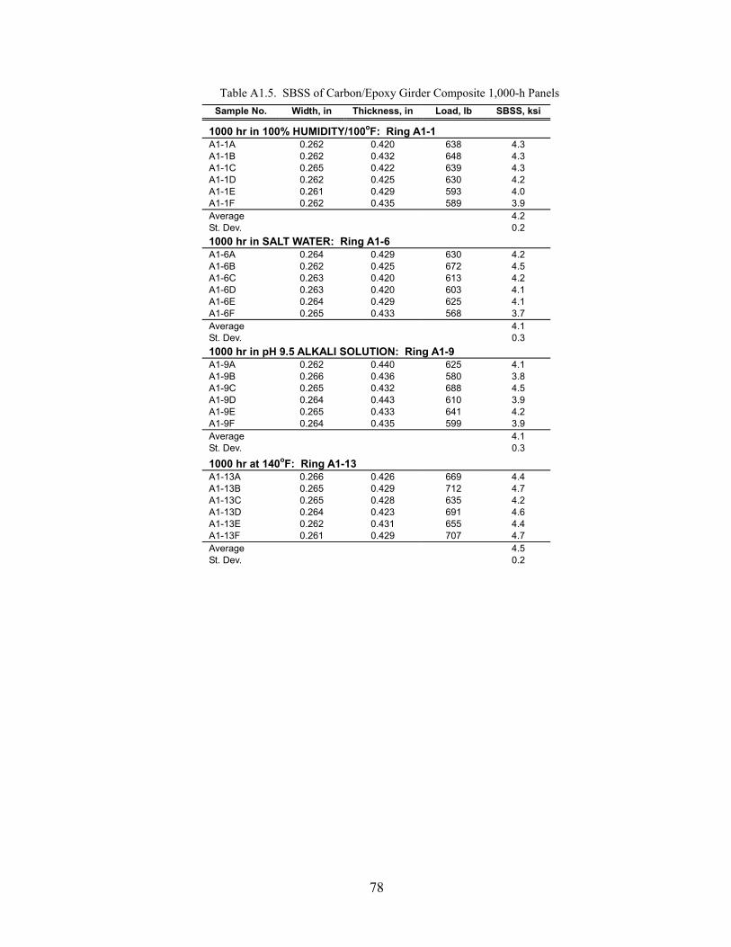
Table A1.5. SBSS of Carbon/Epoxy Girder Composite 1,000-h Panels Sample No. Width, in Thickness, in Load, lb SBSS, ksi

1000 hr in 100% HUMIDITY/100oF: Ring A1-1 A1-1A 0.262 0.420 638 4.3 A1-1B 0.262 0.432 648 4.3 A1-1C 0.265 0.422 639 4.3 A1-1D 0.262 0.425 630 4.2 A1-1E 0.261 0.429 593 4.0 A1-1F 0.262 0.435 589 3.9 Average 4.2 St. Dev. 0.2 1000 hr in SALT WATER: Ring A1-6 A1-6A 0.264 0.429 630 4.2 A1-6B 0.262 0.425 672 4.5 A1-6C 0.263 0.420 613 4.2 A1-6D 0.263 0.420 603 4.1 A1-6E 0.264 0.429 625 4.1 A1-6F 0.265 0.433 568 3.7 Average 4.1 St. Dev. 0.3 1000 hr in pH 9.5 ALKALI SOLUTION: Ring A1-9 A1-9A 0.262 0.440 625 4.1 A1-9B 0.266 0.436 580 3.8 A1-9C 0.265 0.432 688 4.5 A1-9D 0.264 0.443 610 3.9 A1-9E 0.265 0.433 641 4.2 A1-9F 0.264 0.435 599 3.9 Average 4.1 St. Dev. 0.3 1000 hr at 140oF: Ring A1-13 A1-13A 0.266 0.426 669 4.4 A1-13B 0.265 0.429 712 4.7 A1-13C 0.265 0.428 635 4.2 A1-13D 0.264 0.423 691 4.6 A1-13E 0.262 0.431 655 4.4 A1-13F 0.261 0.429 707 4.7 Average 4.5 St. Dev. 0.2

78


3000 hr in 100% HUMIDITY/100oF: Ring A1-2 A1-2A 0.267 0.426 606 4.0 A1-2B 0.271 0.422 639 4.2 A1-2C 0.269 0.429 654 4.3 A1-2D 0.271 0.428 727 4.7 A1-2E 0.272 0.427 693 4.5 A1-2F 0.269 0.436 638 4.1 Average 4.3 St. Dev. 0.3 3000 hr in SALT WATER: Ring A1-7 A1-7A 0.265 0.431 638 4.2 A1-7B 0.267 0.430 608 4.0 A1-7C 0.263 0.441 672 4.3 A1-7D 0.268 0.430 688 4.5 A1-7E 0.262 0.425 643 4.3 A1-7F 0.274 0.427 649 4.2 Average 4.2 St. Dev. 0.2 3000 hr in pH 9.5 ALKALI SOLUTION: Ring A1-10 A1-10A 0.273 0.425 613 3.9 A1-10B 0.256 0.438 570 4.3 A1-10C 0.271 0.425 669 4.3 A1-10D 0.271 0.421 644 4.8 A1-10E 0.271 0.424 670 4.5 A1-10F 0.257 0.431 608 4.3 Average 4.3 St. Dev. 0.3 3000 hr at 140oF: Ring A1-14 A1-14A 0.270 0.426 670 4.4 A1-14B 0.268 0.426 664 4.4 A1-14C 0.268 0.426 636 4.2 A1-14D 0.269 0.425 620 4.1 A1-14E 0.267 0.427 700 4.6 A1-14F 0.272 0.428 600 3.9 Average 4.2 St. Dev. 0.3

79


10,000 hr in 100% HUMIDITY/100oF: Ring A1-3 A1-3A 0.281 0.439 713 4.3 A1-3B 0.279 0.438 776 4.8 A1-3C 0.281 0.438 708

Average

4.3 A1-3D 0.279 0.438 674 4.1 A1-3E 0.282 0.432 696 4.3 A1-3F 0.281 0.436 790 4.8

4.4 St. Dev. 0.3 10,000 hr in SALT WATER: Ring A1-8 A1-8A 0.283 0.426 678 4.2 A1-8B 0.282 0.431 746 4.6 A1-8C 0.283 0.420 701 4.4 A1-8E 0.281 0.430 720 4.5 A1-8F 0.279 0.425 653 4.1 A1-8G 0.279 0.428 680 4.3 Average 4.4 St. Dev. 0.2 10,000 hr in pH 9.5 ALKALI SOLUTION: Ring A1-11 A1-11A 0.270 0.421 620 4.7 A1-11B 0.272 0.431 664 5.0 A1-11C 0.276 0.426 762 4.5 A1-11D 0.270 0.423 638 4.4 A1-11E 0.273 0.423 660 4.5 A1-11F 0.273 0.430 651 5.0 Average 4.7 St. Dev. 0.3

80

Table A1.8. SBSS of Carbon/Epoxy Girder Composite Exposure Panels Sample No. Width, in Thickness, in Load, lb SBSS, ksi

20 FREEZE/THAW CYCLES: Ring A1-4 A1-4A 0.262 0.435 560 3.7 A1-4B 0.258 0.430 550 3.7 A1-4C 0.256 0.434 514 3.5 A1-4D 0.259 0.435 558 3.7 A1-4E 0.256 0.438 641 4.3 A1-4F 0.255 0.436 670 4.5 Average 3.9 St. Dev.

508

0.4 4 hr in DIESEL FUEL: Ring A1-16 A1-16B 0.248 0.429 3.6 A1-16C 0.252 0.432 575 4.0 A1-16D 0.246 0.422 610 4.4 A1-16E 0.252

0.251

0.432 672 4.6 A1-16F 0.250 0.427 613 4.3 A1-16G 0.427 639 4.5 Average 4.2 St. Dev. 0.4 UV CONDENSATION for 100 CYCLES: Ring A1-17 A1-17A 0.279 0.443 700 4.2

0.424 636 4.0 A1-17C 634 4.0 A1-17D 0.278 705 4.4 A1-17E 0.277 0.438 670 4.1 A1-17F 0.265 0.422 702 4.7 Average 4.2 St. Dev. 0.3

A1-17B 0.281 0.281 0.427

0.434

81

Table A1.9. Hardness of Carbon/Epoxy Girder Composite Panels CONTROL PANELS 100% HUMIDITY/100 F 1000 Hr 3000 Hr 10,000 Hr A01-2M A03-3M A01-4F A03-2A A01-1F A01-1M A01-1A 92 90 91 91 94 94 90 92 90 93 84 94 95 87 92 91 95 94 91 92 90 86 90 90 90 87 92 91

85 92 94 82 88 85 90 86 92 93 90 87 94 81

Average 89 91 93 89 90 92 88 St. Dev. 3 1 2 5 3 4 4 Cum. Avg. 90 St. Dev. 3

DRY HEAT AT 140 F FREEZE/THAW SALT WATER 1000 Hr 3000 Hr 20 Cycles 1000 Hr 3000 Hr 10,000 Hr A01-4M A01-4A A01-2F A01-3F A01-3M A01-3A 88 94 94 92 95 90 92 94 92 90 93 82 93 94 93 92 91 91 88 92 86 85 92 87 88 92 90 84 93 83 88 91 86 89

Average 90 93 90 88 91

89 93 87 St. Dev. 2 1 3 3 2 4

pH 9.5 ALKALI SOLUTION DIESEL FUEL UV/COND. 1000 Hr 3000 Hr 10,000 Hr 4 Hr 800

Cycles A03-1A A03-1F A03-1M A01-2A A01-2A 93 93 88 87 95 All on 89 86 85 92 92 Exposure 94 92 90 93 90 Side 90 89 93 86 80 91 93 84 90 91 90 93 90 92 87

Average 91 91 88 90 89 St. Dev. 2 3 3 3 5

82

Appendix 2—Tabulated Data for Individual Tensile, Hardness, and Bondline LSS Measurements for the Kings Stormwater Bridge E-glass/Epoxy Vinyl Ester Deck-Reinforcement Composite

83

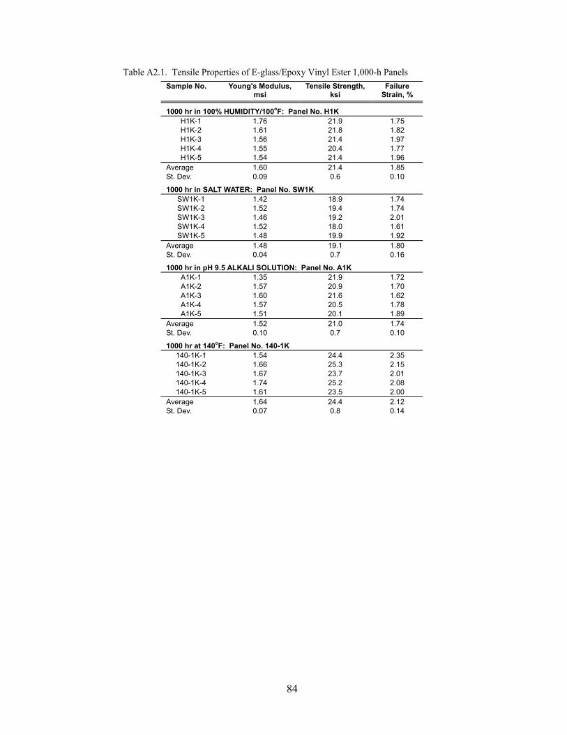
Table A2.1. Tensile Properties of E-glass/Epoxy Vinyl Ester 1,000-h Panels Sample No. Young's Modulus,


ksi Failure

Strain, %

1000 hr in 100% HUMIDITY/100oF: Panel No. H1K

H1K-1 1.76 21.9 1.75 H1K-2 1.61 21.8 1.82 H1K-3 1.56 21.4 1.97 H1K-4 1.55 20.4 1.77 H1K-5 1.54 21.4 1.96

Average 1.60 21.4 1.85 St. Dev. 0.09 0.6 0.10

1000 hr in SALT WATER: Panel No. SW1K SW1K-1 1.42 18.9 1.74 SW1K-2 1.52 19.4 1.74 SW1K-3 1.46 19.2 2.01 SW1K-4 1.52 18.0 1.61 SW1K-5 1.48

1.48 19.9 1.92

Average 19.1 1.80 St. Dev. 0.04

1.72

0.7 0.16

1000 hr in pH 9.5 ALKALI SOLUTION: Panel No. A1K A1K-1 1.35 21.9 A1K-2 1.57 20.9 1.70

1.62 1.78

A1K-5 1.51

A1K-3 1.60 21.6 A1K-4 1.57 20.5

20.1 1.89 Average 1.52 21.0 1.74 St. Dev. 0.10 0.7 0.10

1000 hr at 140oF: Panel No. 140-1K 140-1K-1 1.54 24.4 2.35 140-1K-2 1.66 25.3 2.15 140-1K-3 1.67 23.7 2.01 140-1K-4 1.74 25.2 2.08 140-1K-5 1.61 23.5 2.00

Average 1.64 24.4 2.12 0.07 0.8 0.14 St. Dev.

84



ksi Failure

Strain, %

3000 hr in 100% HUMIDITY/100oF: Panel No. H3K

H3K-1 1.48 16.7 1.38 H3K-2 1.64 18.7 1.59 H3K-3 1.68 18.0 1.65 H3K-4 1.80 17.9 1.53 H3K-5 1.80 17.9 1.63

Average 1.68 17.8 1.56 St. Dev. 0.13 0.7 0.11

3000 hr in SALT WATER: Panel No. SW3K SW3K-1 1.84 20.2 1.80 SW3K-2 1.84 18.7 1.47 SW3K-3 1.60 17.9 1.61 SW3K-4 18.3 SW3K-5 18.1

Average 1.76 18.6 1.63 St. Dev. 0.14 0.9 0.17

3000 hr in pH 9.5 ALKALI SOLUTION: Panel No. A3K A3K-1 A3K-2 1.51 20.3 1.79 A3K-3 1.55 19.4 1.71 A3K-4 1.55 16.8 1.34 A3K-5 1.51 17.8 1.48

Average 1.53 18.6 1.58 St. Dev. 0.02 1.6 0.21

3000 hr at 140oF: Panel No. 140-3K 140-3K-1 1.92 20.8 1.67 140-3K-2 1.80 20.0 1.65 140-3K-3 1.92 20.6 1.73 140-3K-4 1.80 19.2 2.11 140-3K-5 1.80 19.2 1.59

Average 1.85 20.0 1.75 St. Dev. 0.07 0.8 0.21

85



ksi Failure

Strain, %

10,000 hr in 100% HUMIDITY/100oF: Panel No. H10K

H10K-1 1.45 16.5 1.42 H10K-2 1.36 15.7 1.44 H10K-3 1.49 16.0 H10K-4 1.47

1.28 16.0 1.36

H10K-5 1.53 16.1 1.33 Average 1.46 16.1 1.37 St. Dev. 0.06 0.3 0.07

10,000 hr in SALT WATER: Panel No. SW10K SW10K-1 1.61 23.8 2.04 SW10K-2 1.57 21.3 1.75 SW10K-3 1.48 21.6 1.98 SW10K-4 1.48 21.2 2.03 SW10K-5 1.35

Average 1.50 20.3 1.94 21.6 1.95 1.3 0.12

A10K-1 1.60 20.1 1.70 A10K-2 1.58 20.4 1.90

20.0 1.77

18.2

A10K-3 1.57 A10K-4 1.63 19.3 1.54 A10K-5 1.45 1.60

Average 1.57 19.6 1.70 St. Dev. 0.07 0.9 0.14

St. Dev. 0.10

10,000 hr in pH 9.5 ALKALI SOLUTION: Panel No. A10K

Table A2.4. Tensile Properties of E-glass/Epoxy Vinyl Ester Exposure Panels

Sample No. Young's Modulus, Failure Strain, % msi

Tensile Strength, ksi

20 Freeze/Thaw Cycles: Panel No. F/T

1.72 17.9 1.51 17.2 1.38

F/T-3 1.64 19.1 1.74 F/T-4 19.0 1.72 F/T-5 18.8 1.99

Average 1.69 18.4 1.67 St. Dev. 0.09 0.8 0.23

4 hr in Diesel Fuel: Panel No. DF DF-1 1.54 21.5 2.00 DF-2 1.56 20.7

20.0 21.0 19.7

1.81 DF-3 1.61 1.72 DF-4 1.56 1.86 DF-5 1.64 1.63

Average 1.58 20.6 1.80 St. Dev. 0.04 0.7 0.14

800 UV/CONDENSATION CYCLES: Panel No. UV UV-1 1.68 21.6 1.77 UV-2 1.59 20.6 1.79 UV-3 1.64 19.4 1.64 UV-4 1.75 22.0 1.73 UV-5 1.62 21.0 1.75

Average 1.66 20.9 1.74 St. Dev. 0.06 1.0 0.06

F/T-1 F/T-2 1.80

1.60

86

Table A2.5. Hardness Data for E-glass/Epoxy Vinyl Ester Panels CONTROL PANELS 100% HUMIDITY/100 F 1,000 h 3,000 h 10,000 h

C1 C2 C3 C4 H1000 H3000 H10000 84 96 90 89 86 90 88 92 93 90 88 92 92 86 89 90 85 88 88 87 86 88 87

90 87 90 93 89 90 88 86 89 88 89 93 91 92 88 87 89

Average 89 89 91 90 88 88 89 St. Dev. 3 2 3 2 2 1 2 Cum. Avg. 90 St. Dev. 3

3,000 h

DRY HEAT AT 140 F FREEZE/THAW SALT WATER 1,000 h 3,000 h 20 CYCLE 1,000 h 10,000 h 140-1000 140-3000 F/T S1000 S3000 S10000 89 94 92 90 90 90 89 92 88 87 87 87 90 92 91 87

86

91 87 90 91 87 90 90 89 90 84 91 90 91 88 93 90 89 88 85

Average 89 91 90 89 90 87 St. Dev. 1 3 2 1

2 2

pH 9.5 ALKALI SOLUTION DIESEL FUEL ASTM G 53 1,000 h 3,000 h 10,000 h 4 h 100 CYCLES A1000 A3000 A10000 UV 90 89 90 87 92 Back Side 90 91 89 87 91 Back Side 90 90 87 84 91 Back Side 89 86 87 94 94 Back Side 92 90 89 90 90 Back Side 91 91 88 92 92 Back Side

Average 90 90 88 89 92 St. Dev. 1 2 1 3 1

90 90

87

Table A2.6. LSS Data for 2,000-h Bonded Assemblies

Sample No. Width, in

Overlap Length, in

Failure Load, lb

Lap Shear Strength, psi Failure Mode

2000 hr in 100% HUMIDITY/100oF: Panel No. MMBA-1C

1C-1 1.040 0.569 1080 1825 Adhesive + Pultrusion mat shear 1C-2 0.983 0.550 960 1776 " 1C-3 0.995 0.556 845 1527 Pultrusion interlaminar shear 1C-4 0.970 0.297 415 1441 Adhesive + Pultrusion mat shear 1C-5 0.894 0.563 700 1391 Pultrusion interlaminar shear


2000 hr in SALT WATER: Panel No. MMBA-2C 2C-1 0.986 0.498 900 1833 Adhesive + Pultrusion mat shear 2C-2 0.987 0.514 1080 2129 " 2C-3 0.996 0.491 1190 2433 " 2C-4 0.988 0.496 1155 2357 " 2C-5 0.981 0.502 885 1797 "


2000 hr in pH 9.5 ALKALI SOLUTION: Panel No. MMBA-3C 3C-1 0.991 0.527 925 1771 Adhesive 3C-2 0.985 0.523 1075 2087 Pultrusion interlaminar shear 3C-3 1.004 0.535 1090 2029 Adhesive + Pultrusion mat shear 3C-4 1.006 0.220 630 2847 " 3C-5 0.996 0.491 775 1585 "


2000 hr at 140oF: Panel No. MMBA-2D 2D-1 0.982 0.432 630 1485 Adhesive + Pultrusion mat shear 2D-2 0.972 0.422 860 2097 " 2D-3 0.987 0.463 1100 2407 " 2D-4 0.965 0.490 880 1861 Hand Lay-up interlaminar shear 2D-5 0.980 0.425 925 2221 Adhesive + Pultrusion mat shear


88



Overlap Length, in

Failure Load, lb


5000 hr in 100% HUMIDITY/100oF: Panel No. MMBA-1A

1A-1 0.987 0.376 1117 3010 Pultrusion interlaminar shear

1A-2 0.993 0.384 394 1033 Bad test, misalignment with tensile axis

1A-3 0.986 0.426 552 1314 " 1A-4 0.989 0.468 474 1024 " 1A-5 0.989 0.488 1165 2414 Pultrusion interlaminar shear 1A-7 0.743 0.432 545 1698 " 1A-8 0.753 0.425 909 2840 "


5000 hr in SALT WATER: Panel No. MMBA-2A 2A-1 0.985 0.398 632 1612 Pultrusion mat shear

2A-2 0.988 0.438 893 2064 Pultrusion interlaminar shear + mat shear

2A-3 0.991 0.446 969 2192 Pultrusion interlaminar shear 2A-4 0.996 0.463 1060 2299 Pultrusion mat shear 2A-5 0.991 0.443 1010 2301 Pultrusion interlaminar shear


5000 hr in pH 9.5 ALKALI SOLUTION: Panel No. MMBA-3A 3A-1 0.971 0.421 867 2121 Pultrusion interlaminar shear 3A-2 0.980 0.448 626 1426 " 3A-3 0.981 0.425 874 2096 Pultrusion mat shear

3A-4 0.993 0.451 1002 2237 Pultrusion interlaminar shear + mat shear

3A-5 0.988 0.490 1086 2243 Pultrusion interlaminar shear Average 2025 St. Dev. 341

5000 hr at 140oF: Panel No. MMBA-5A 5A-1 0.989 0.495 1248 2549 Pultrusion interlaminar shear 5A-2 0.997 0.481 940 1960 " 5A-3 0.997 0.480 733 1532 " 5A-4 0.987 0.496 664 1356 " 5A-5 0.995 0.529 1258 2390 "


89

90



Overlap Length, in

Failure Load, lb


12,910 hr in 100% HUMIDITY/100oF: Panel No. MMBA-1B

1B-1 0.962 0.472 1112 2449 Pultrusion interlaminar shear + mat shear

1B-2 0.966 0.470 1093 2407 " 1B-3 0.965 0.483 1000 2145 " 1B-4 0.954 0.463 935 2117 " 1B-5 0.962 0.459 977 2213 Pultrusion interlaminar shear


12,910 hr in SALT WATER: Panel No. MMBA-2B 2B-1 0.989 0.572 969 1713 Pultrusion mat shear 2B-2 0.994 0.540 993 1850 " 2B-3 0.998 0.544 1126 2074 Pultrusion interlaminar shear

2B-4 0.990 0.517 1150 2247 Pultrusion interlaminar shear + mat shear

2B-5 0.992 0.502 1098 2205 Pultrusion mat shear Average 2018 St. Dev. 230

12,910 hr in pH 9.5 ALKALI SOLUTION: Panel No. MMBA-3B 3B-1 0.956 0.463 989 2234 Pultrusion interlaminar shear 3B-2 0.966 0.458 895 2023 " 3B-3 0.971 0.497 1089 2257 " 3B-4 0.972 0.485 892 1892 " 3B-5 0.967 0.480 967 2083 "


Table A2.9. LSS Data for Freeze/Thaw Bonded Assembly


Overlap Length, in

Failure Load, lb


20 Freeze/Thaw Cycles: Panel No. MMBA-4A 4A-1 Pultrusion interlaminar shear 4A-2 0.986 0.547 1175 2179 " 4A-3 0.989 0.535 1165 2202 " 4A-4 0.992 0.475 1040 2207 " 4A-5 0.991 0.483 1215 2538 "


the application of qualification testing, field … · aerospace report no. atr-2005(7796)-1 the...

Documents