THE APPLICATION OF SHADING MASKS IN BUILDING SIMULATION

Dr. Andrew Marsh Welsh School of Architecture, Cardiff University, Cardiff, UK

& Square One research, Australia www.squ1.com andrew@squ1.com

ABSTRACT

Calculating the dynamic effects of surface overshadowing is a major part of most thermal analysis engines. It also represents a significant overhead in the analysis process yet, once a run is complete, this information is usually lost and must be entirely recalculated before the next run. However, detailed overshadowing for specific surfaces is valuable information to the designer. It is also useful for many other forms of building performance analysis such as detailed shading design, material selection, daylighting, right-to-light and even solar-access calculations.

This paper proposes the widespread use of pre-calculated shading masks in thermal analysis engines. It discusses why this is important, the different techniques for calculating and storing these masks as well as the benefits and disadvantages of different methods. A comparison of both the accuracy and computational overhead of different sky-subdivision techniques is also presented. More importantly, it shows that complex effects such as solar reflection and incidence effects can be accommodated within the masks themselves and how they can also be used in the calculation of average daylight factors, glare potential, radiant exchange and even internal surface solar tracking.

INTRODUCTION Incident solar radiation (insolation) on external surfaces is a major influence on a building’s overall performance, impacting on internal comfort, energy use, lighting and even general amenity. The accurate calculation of insolation is fundamental to thermal simulation tools and a whole range of different techniques have been developed for this purpose. However, within these differences often lie problems of access and inflexibility.

In many tools, the calculation of detailed shading effects is computationally expensive, requiring that each shading device be explicitly defined and a whole range of cached data generated for each surface within the model. This cached data is then discarded at the end of the analysis run.

From a designer’s perspective, detailed shading data for each surface in a model represents a wealth of potential design information. If visualised in an appropriate way - mapped over a sun-path diagram for example - it can immediately show exactly when a surface is in shade, by what and for how long. This in itself can form the basis of many important design decisions.

However, none of the major freely available thermal analysis tools such as EnergyPlus (Crawley et.al. 2004) allow access to this detailed information, other than through some simplified summary data or single time-specific values. Also, because the calculations are usually done internally in each tool, the effect of complex shading devices must be approximated or modelled abstractly using the often quite limited techniques and geometric primitives the tool provides. This lack of modelling control, coupled with the inability to view in detail what the final effect is, often means that shading is treated quite cursorily in many instances.

This paper proposes the use of shading masks as a solution to these problems. As described later, shading masks allow for detailed shading information to be stored between runs and should ideally be done in a format that other tools can view, edit or even generate. Using shading information this way has the following potential benefits:

%

100

90

80

70

60

50

40

30

20

10

0

N15°

30°

45°

60°

75°

90°

105°

120°

135°

150°

165°180°

195°

210°

225°

240°

255°

270°

285°

300°

315°

330°

345°

10°

20°

30°

40°

50°

60°

70°

80°

4

5

6

7

8

910111213

1415

16

17

18

19

20

1st Jan

1st Feb

1st M ar

1st Apr

1st M ay

1st Jun1st Ju l

1st Aug

1st Sep

1st Oc t

1st N ov

1st D ec

Stereographic Diagram Loc ation: 51.4°, 0.0°

Ob j 6589 Orienta tion: -90 .3°, 0 .0° Sun Position: -167.4°, 27.0° H SA: -77.1°

VSA: 66.3°

T ime: 12:30 D ate: 22nd Oc t (295)

Perc entage Shad ing: 0 %

BR E VSC: 20.7%Ov erc ast Sk y Fac tor: 20 .7%

U niform Sk y Fac tor: 20 .7%

Figure 1 An example shading mask generated for an overshadowed window in London mapped

over a sun-path diagram.

Ninth International IBPSA Conference Montréal, Canada

August 15-18, 2005

- 725 -

• Shading masks need recalculation only when the actual building or site geometry changes. The same masks can be used for any orientation, calculation period, location and, if reflection data is not stored directly, are even tolerant of changes in material and surface properties.

• Complex shading situations that may not be easily modelled within one particular analysis tool could easily be generated within another and applied to relatively simple surfaces with the same effect.

• Where complex CAD models of the site are available, there would be no need to modify and import this into the analysis tool itself, thereby significantly reducing the overheads and complexity of the analysis model. With the right shading masks, the same (if not greater) accuracy could be achieved, resulting in much simpler and faster thermal models.

• Being able to visualise and even create the shading input means the designer knows exactly what the calculation is based on, making it easier to track down anomalous results and control the level of detail to their own specific requirements.

• Future tools could support multiple shading masks representing different environmental conditions. These could then be applied to objects at different times during a calculation to accurately simulate dynamic events such as deciduous vegetation or complex moveable shading devices.

With computational analysis fast becoming an important part of the entire design process, not just as a final validation tool, the flexibility to control, store and view this kind of information is increasingly important. Also, in performance-driven design processes and parametric analysis, the same model may be run many thousands of times so any reduction in calculation time through the caching of shading data is vitally important.

SHADING MASKS A shading mask is simply a mechanism for recording which parts of the sky are visible from a particular point in the model and which are not. For any given set of obstructions, this information can be overlaid on a sun-path diagram to show when in the year the point is in shade or not.

Whilst this diagram can be generated by projecting obstructing surfaces back towards the point from which the mask is generated, and drawing a series of

transformed polygons (as shown in Figure 2 – left side), it is more useful for numerical analysis to divide the sky into discrete segments and simply store shading values for each one (as shown in Figure 2 – right side). Once segmented in this way, information can be obtained quickly by simply referencing all or parts of the mask directly.

A major benefit of using the sky segment approach is that each segment can store quite complex data. As shown above, the shading mask for a single point is hard edged - it is either in shade or not. However, a shading mask for a planar surface is usually soft-edged as the surface may only be partially in shade at a particular time.

One of the simplest ways of determining the partial shading of a surface is to sample it as a series of distributed points and average the results into a single mask. This way each segment can be used to store fractional obstruction values or a shading percentage.

Figure 3 shows how the shading percentage for any sky segment can be calculated by spraying rays out from a number of sample points on a surface and then determining the percentage that were obstructed by surrounding objects. If this is done for all sky segments, an image of the occlusion of the sky from that surface can be generated, shown here as the soft-edged shading mask to the right of Figure 3.

Figure 2 Example shading masks for window centre, showing shading polygons (left) and the sky

dome divided into discrete segments (right).

Figure 3 Shading masks for planar surfaces must

store fractional shading information.

- 726 -

Instantaneous Insolation

The calculation of insolation on a surface involves several steps, including both geometric occlusion and the solution of many trigonometric equations which are quite processor intensive. Whilst the shading mask is a useful means of caching occlusion data so that it does not need to be recalculated many times, it has the additional benefit of eliminating a significant number of trigonometric functions in each analysis, resulting in a further reduction in calculation times.

Insolation depends on the angle of incidence at which radiation strikes each surface, calculated using the cosine law in which radiation arriving normal to the surface has a greater effect than that arriving at grazing incidence. Thus, for the direct solar component, the angle between the position of the Sun and each surface’s normal must be known at each time-step. For hourly calculations over the whole year this will require as many as 4380 solutions for each object in the model (sunrise to sunset) – many more for sub-hourly time-steps.

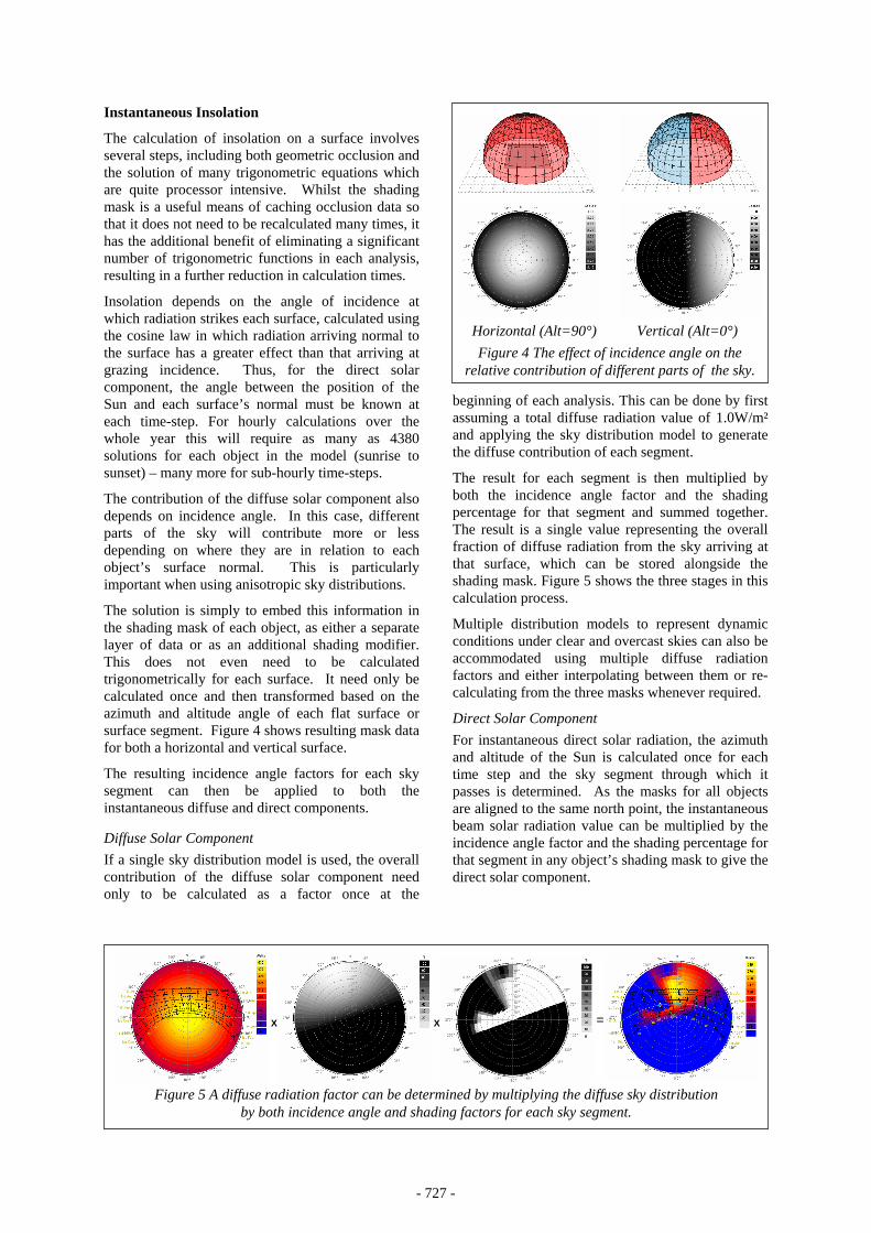
The contribution of the diffuse solar component also depends on incidence angle. In this case, different parts of the sky will contribute more or less depending on where they are in relation to each object’s surface normal. This is particularly important when using anisotropic sky distributions.

The solution is simply to embed this information in the shading mask of each object, as either a separate layer of data or as an additional shading modifier. This does not even need to be calculated trigonometrically for each surface. It need only be calculated once and then transformed based on the azimuth and altitude angle of each flat surface or surface segment. Figure 4 shows resulting mask data for both a horizontal and vertical surface.

The resulting incidence angle factors for each sky segment can then be applied to both the instantaneous diffuse and direct components.

Diffuse Solar Component If a single sky distribution model is used, the overall contribution of the diffuse solar component need only to be calculated as a factor once at the

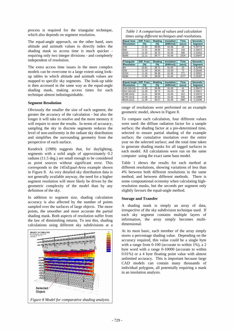
beginning of each analysis. This can be done by first assuming a total diffuse radiation value of 1.0W/m² and applying the sky distribution model to generate the diffuse contribution of each segment.

The result for each segment is then multiplied by both the incidence angle factor and the shading percentage for that segment and summed together. The result is a single value representing the overall fraction of diffuse radiation from the sky arriving at that surface, which can be stored alongside the shading mask. Figure 5 shows the three stages in this calculation process.

Multiple distribution models to represent dynamic conditions under clear and overcast skies can also be accommodated using multiple diffuse radiation factors and either interpolating between them or re-calculating from the three masks whenever required.

Direct Solar Component For instantaneous direct solar radiation, the azimuth and altitude of the Sun is calculated once for each time step and the sky segment through which it passes is determined. As the masks for all objects are aligned to the same north point, the instantaneous beam solar radiation value can be multiplied by the incidence angle factor and the shading percentage for that segment in any object’s shading mask to give the direct solar component.

Horizontal (Alt=90°) Vertical (Alt=0°) Figure 4 The effect of incidence angle on the

relative contribution of different parts of the sky.

X X =

Figure 5 A diffuse radiation factor can be determined by multiplying the diffuse sky distribution by both incidence angle and shading factors for each sky segment.

- 727 -

Cumulative Insolation

Whilst not usually required in a thermal analysis calculation, it can often be useful to know the total solar collection on a surface over an extended time period. This can be achieved very simply using the same technique, but this time with a cumulative sky generated by aggregating the total solar radiation passing through each sky segment over the chosen calculation period.

To generate a cumulative sky, each hourly or sub-hourly diffuse sky distribution is summed for each segment over the calculation period. At the same time, the Sun position at each time-step is used to determine the sky segment to which the beam radiation is added. Because all the geometric analysis is already embedded in the masks themselves, a single cumulative sky array can be used to very quickly calculate and display the relative solar exposure over all objects in even the most complex model. As this involves simple multiplication of data arrays, this can even be done in close to real time.

An example of such a cumulative sky distribution is shown in the left-most image in Figure 6. In this case, taken over the entire year, the direct component clearly dominates the resulting cumulative sky distribution.

PRACTICAL CONSIDERATIONS

Sky Subdivision

There are many ways to subdivide the sky dome into discrete segments. Some seek to achieve a roughly equal-area (solid angle) for each segments whilst others apply a simpler latitude/longitude or equal-angle approach. Figure 7 shows some examples of different techniques as well as how the resolution can vary.

The methods used to generate these different subdivisions have been widely published (White, et. al. 1998, Tregenza, 1995 and Wenninger, 1999) so will not be covered here. However, given that it is possible to weight each sky segment by its relative area compared to all others, it is not actually necessary that each segment be of even close to equivalent size. It is therefore more practical

considerations that will influence the choice of technique.

Access Times

Once the shading mask for a surface has been pre-calculated, it’s data must be accessed many times during the analysis process, typically once per time-step. As previously discussed, this can be 4380 or more times for each object in an annual calculation. Thus, the processor time spent accessing the shading mask is an important consideration as different techniques vary significantly.

For equal-area techniques, the procedure for finding the right segment index given an altitude and azimuth for the Sun involves an iterative solution in which the number of step depends on the segment resolution (Tregenza, 1995). A similarly complex

145 x Equal-Area 580 x Equal-Area

256 x Triangular 1024 x Triangular

324 x Equal-Angle (10°) 1296 x Equal-Angle (5°)

Figure 7 Some examples of different sky subdivision techniques.

X X =

Figure 6 Total solar collection can be calculated using a cumulative sky, in which solar radiation through each segment is aggregated over time and then multiplied by incidence angle and shading factors.

- 728 -

process is required for the triangular technique, which also depends on segment resolution.

The equal-angle approach, on the other hand, uses altitude and azimuth values to directly index the shading mask so access time is much quicker - requiring only two integer divisions - and completely independent of resolution.

The extra access time issues in the more complex models can be overcome to a large extent using look-up tables in which altitude and azimuth values are mapped to specific sky segments. The look-up table is then accessed in the same way as the equal-angle shading mask, making access times for each technique almost indistinguishable.

Segment Resolution

Obviously the smaller the size of each segment, the greater the accuracy of the calculation - but also the longer it will take to resolve and the more memory it will require to store the results. In terms of accuracy, sampling the sky in discrete segments reduces the level of non-uniformity in the radiant sky distribution and simplifies the surrounding geometry from the perspective of each surface.

Kendrick (1989) suggests that, for daylighting, segments with a solid angle of approximately 0.2 radians (11.5 deg.) are small enough to be considered as point sources without significant error. This corresponds to the 145xEqual-Area example shown in Figure 8. As very detailed sky distribution data is not generally available anyway, the need for a higher segment resolution will more likely be driven by the geometric complexity of the model than by any definition of the sky.

In addition to segment size, shading calculation accuracy is also affected by the number of points sampled over the surfaces of large objects. The more points, the smoother and more accurate the partial shading mask. Both aspects of resolution suffer from the law of diminishing returns. To test this, shading calculations using different sky subdivisions at a

range of resolutions were performed on an example geometric model, shown in Figure 8.

To compare each calculation, four different values were used: the diffuse radiation factor for a sample surface; the shading factor at a pre-determined time, selected to ensure partial shading of the example surface; the cumulative insolation over the entire year on the selected surface; and the total time taken to generate shading masks for all tagged surfaces in each model. All calculations were run on the same computer using the exact same base model.

Table 1 shows the results for each method at different resolutions, showing variations of less than 4% between both different resolutions in the same method, and between different methods. There is some computational economy when calculating high-resolution masks, but the seconds per segment only slightly favours the equal-angle method.

Storage and Transfer

A shading mask is simply an array of data, irrespective of the sky subdivision technique used. If each sky segment contains multiple layers of information, the array simply becomes multi-dimensional.

At its most basic, each member of the array simply stores a percentage shading value. Depending on the accuracy required, this value could be a single byte with a range from 0-100 (accurate to within 1%), a 2 byte word with a range 0-10000 (accurate to within 0.01%) or a 4 byte floating point value with almost unlimited accuracy. This is important because large CAD models can contain many thousands of individual polygons, all potentially requiring a mask in an insolation analysis.

Figure 8 Model for comparative shading analysis.

Table 1 A comparison of values and calculation times using different techniques and resolutions.

Equal Area Diff. Fract. Shading Insolation Time Seconds /Resolution (%) (%) (kWh/m2) (secs) Segment145 11.33 38.83 61.65 43 0.29773580 11.31 38.85 61.65 156 0.268732320 11.45 38.70 61.65 586 0.252639280 11.11 38.77 61.65 2324 0.25047

Triangular Diff. Fract. Shading Insolation Time Seconds /Resolution (%) (%) (kWh/m2) (secs) Segment64 10.91 38.71 61.65 20 0.31456256 11.33 38.94 61.65 72 0.281651024 11.34 38.48 61.65 271 0.265014096 11.05 38.69 61.65 1077 0.26287

Equal-Angle Diff. Fract. Shading Insolation Time Seconds /Resolution (%) (%) (kWh/m2) (secs) Segment144 (15x15) 11.30 38.89 61.65 41 0.28472324 (10x10) 11.28 38.75 61.65 83 0.256171296 (5x5) 11.41 38.65 61.65 312 0.240742700 (4x3) 11.06 38.54 61.65 645 0.238898100 (2x2) 11.09 38.57 61.65 1887 0.23296

- 729 -

Table 2 The number of bytes required to store shading masks of different resolutions & accuracy.

Bytes 145 580 2320 92801 145 580 2320 92802 290 1160 4640 185604 580 2320 9280 37120

Sky Segments

Table 2 shows the rapid increase in memory size required to store shading masks with different segment resolutions and accuracies. At its highest level, this can be as much as 37 kilobytes per mask layer per object. For a 1,000 object model, this equates to 37 megabytes, compared to just 145 kilobytes for the lowest resolution and accuracy.

When used internally within an analysis tool, the exact storage method is not particularly important as machine memory is usually more than sufficient. However, if used by external tools, the format in which they are stored does become important.

Here too there is a trade-off. The aim is obviously for a flexible and universally accessible format - preferably human readable - which can accomm-odate the many different sky subdivision, resolution and accuracy options. The use of an XML schema for example would simplify the development of viewers or editors and offer just such a universal and readable format.

However, the requirement to include a validating XML parser would add a significant overhead to those analysis tools that must read and write many thousands of masks during a single calculation run. Moreover, a flexible and readable XML format would add a significant number of extra characters to the file which, when storing many thousands of masks, would greatly increase the amount of storage space required. Much of this could be overcome using file compression, however this defeats the very purpose of using a text-based format.

When considering shading as design information, the designer is usually only interested in a relatively small number of surfaces (assuming that most of the objects in the model form the surrounding urban environment that actually does the shading). This suggests that the requirement is really two-fold - in that there is a need for:

- a flexible transfer format for single or small numbers of individual masks, selectively accessed by the user for editing or email, and

- a long-term, optimised and high-volume format for storing large numbers of masks for access during calculations.

Typically long-term, high-volume formats are determined by each tool’s individual requirements, are stored locally (usually alongside the actual

model) and are not flexible in terms of the types of shading masks they can store. However, once a suitably flexible XML schema is developed, it would be possible to develop a compatible database table format with the same field structure.

Masks could then be stored in a central database for access by many different tools. This would eliminate much of the storage overhead of the XML format whilst providing a fast searchable method that is shareable amongst groups of analysts and designers. With the right set of SQL search criteria, it would also be possible for any member of the team to identify surfaces above or below particular exposure limits, etc, from the database alone.

As a result, work is currently underway on both the development of a flexible XML schema for exchanging shading mask data and a compatible but optimised SQL table format for more efficient storage and access to this data.

OTHER DESIGN APPLICATIONS

In addition to accelerating thermal calculations, shading masks have many other uses. Figure 1 not only shows how shading masks can be visualised, but also shows how values such as sky components (overcast sky) and sky factors (uniform sky) can be determined directly from the shading information (shown as text in the bottom-right corner). If the appropriate room properties are known, each window’s shading mask can be used to accurately calculate average daylight factor values (Tregenza, 1995, Algorithm 2.12) and even mean vertical obstruction angles.

By layering additional data in each sky segment, the application of shading masks can be extended further to include the following.

Reflected Solar Radiation Within a shading mask it is also possible to accommodate the effects of specular reflection off surfaces in the surrounding environment. This can be done by spawning reflected rays at each intersection with an obstructing surface, and then tracing each ray until finally unobstructed. At this point the sky segment through which the final spawned ray passes is calculated from the altitude and azimuth of the ray, as shown in Figure 9. The value contributed by each reflected ray to that sky segment is determined by multiplying the reflectance and specularity values of each surface struck, and then dividing the result by the total number of sampled rays generated over the surface of the original object being shaded. The final values of each ray are summed within each sky segment intersected. This means that it is theoretically possible for the fractional value in a particular sky segment to be greater than one. This can occur when

- 730 -

many obstructions focus specular reflections at the same point, effectively magnifying the solar intensity there.

Diffuse reflections are slightly more complex to accommodate. In addition to shading data, a direct reference to the obstructing surface(s) for each sky segment can also be stored. This works best when dealing with single point masks as there is only ever one obstructing object in each direction. In the case of large surfaces it is certainly possible to store multiple objects and the fraction of rays hit, however this has not been attempted or investigated at this stage.

This means that the shading mask can effectively store dynamic information related to each surrounding object. Thus, using their own shading masks, it is possible to calculate the instantaneous incident radiation on every surface in the model, and then perform a second iteration in which object references in each mask are used to determine the radiant exchange between surfaces. This is a well known process used in radiosity-based lighting analysis tools - the shading mask simply serving again as storage for calculated data.

Internal Solar Tracking

Shading masks can also be used to easily track solar radiation through windows and appertures and onto the internal surfaces within a space. To do this, masks are generated from both sides of all building surfaces, even those that are completely internal. Most of the rays sprayed on the internal side will be obstructed by the surfaces that form the envelope of each space, however some will escape out through windows and appertures. Thus, it is possible to determine the percentage in shade for each internal surface for any particular time and, based on its surface area, the effective area exposed to the Sun. Figure 10 shows an example shading mask for a floor object with windows on the north and east facades.

The instantaneous insolation on internal surfaces is found by summing the direct and diffuse solar gains through all of the windows and appertures in the space, and dividing the result by the total effective

exposed area. Given that the shading mask already accounts for incidence angle and external obstruction, as well as the transparencies and shading coefficients of each apperture, the result is a W/m2 value that can be multiplied by the effective exposed area of each surface to give the instantaneous insolation.

This information can then be used, along with the material properties of each surface, to determine how much of the insolation is absorbed into the fabric and how much becomes an instantaneous space load. By dividing internal surfaces up into smaller sub-surfaces, it is also possible to determine the exact location of Sun-patches and to more accurately calculate the spatial distribution of surface temperatures for detailed radiant temperature analysis.

Mean Radiant Temperatures

If object references are included in the shading masks for a grid of analysis points distributed within a space, it is then possible to dynamically calculate mean radiant conditions at each point based on the changing surface temperature of surrounding objects. Used in conjunction with the internal solar tracking capability and subdivided surfaces, this can yield a highly accurate and dynamic simulation of spatial comfort.

Such a system has been implemented as part of this work to calculate the distribution of mean radiant temperatures based on the proximity of objects to each point on an analysis grid. In this case, each shading mask segment stores the object index of each obstruction in each direction and its distance from the point. In the example shown in Figure 11, hourly surface temperatures for a whole day can be stored for each object, allowing time-based recalculations to be performed fast enough for the distribution to be animated dynamically.

Figure 9 It is also possible to calculate and store

reflected solar radiation in a shading mask.

Figure 10 An example shading mask for an internal floor surface with windows along the northern and

eastern facades.

- 731 -

Dynamic Shading Conditions

With the increasing use of operable shading devices and solar controls linked to building management systems, many analysts require the ability to model dynamic shading conditions. The use of shading masks makes this a relatively simple process whereby a schedule can be used to transition between shading masks at different times of the year or even different hours of the day.

Most thermal analysis tools already use schedules to change single parameter values, either in discrete steps or as fractional interpolations between two extremes. This same approach can be applied to shading masks. If a separate indexed list of shading masks is kept, then the schedule could either switch the index assigned to any object at any time, or interpolate between shading values stored in two different masks, as shown in Figure 12.

CONCLUSION The concept of the shading mask is certainly not new. In fact most thermal analysis tools already include many aspects of their implementation. However, the bulk of the shading data these tools generate is inaccessible and too readily discarded. This paper has shown that the use of shading masks and the ability to share them between tools can have significant potential benefits.

These benefits are not solely in terms of calculation speed, though this is an important concern. The extra information and insight offered to designers and the modelling flexibility shading masks provide are equally if not more important.

REFERENCES Crawley, D.B., Lawrie, L.K., Pedersen, C.O.,

Winkelmann, F.C. 2004, EnergyPlus: New, Capable and Linked. Proceedings of the World Renewable Energy Congress VIII, August 29-September 3 2004, Denver, Colorado, USA.

Kendrick, J.D. (Ed.), 1989. Guide to recommended practice of daylight measurement. Commission Internationale de l'Eclairage, Vienna.

Tregenza, P.R., Sharples, S. 1995, IEA Task 21, Subtask C2 - New Daylight Algorithms, (http://eande.lbl.gov/Task21/BRE-ETSU/contents.html).

Wenninger, M., 1999. Spherical Models, Dover Publications, Mineola, NY (USA).

White D.; Kimerling A.J.; Sahr K.; Song L., 1998. Comparing area and shape distortion on polyhedral-based recursive partitions of the sphere, International Journal of Geographical Information Science, vol. 12, no. 8.

Figure 11 Shading masks can be modified to include object proximity data for dynamic radiant

temperature and comfort calculations.

Figure 12 The effect of dynamic shading devices

and deciduous vegetation on object shading masks.

- 732 -