the application of stochastic mesh method in bsdes
TRANSCRIPT

THE APPLICATION OF STOCHASTIC MESH METHOD IN BSDES
XIA HAOYANG(B.S. & B.A., Beijing Normal University)
A THESIS SUBMITTEDFOR THE DEGREE OF MASTER OF SCIENCE
DEPARTMENT OF MATHEMATICSNATIONAL UNIVERSITY OF SINGAPORE
2015

Declaration
I hereby declare that this thesis is my original work and it has been written by me in itsentirety. I have duly acknowledged all the sources of information which have been used in
the thesis.
This thesis has also not been submitted for any degree in any university previously.
October 25, 2015
i

Contents
1 Introduction 1
2 Stochastic mesh method in American option pricing 3
2.1 Estimators . . . . . . . . . . . . . . . . . . . . . . . . . . . . . . . . . . . . . . . . . . 4
2.1.1 Mesh estimator . . . . . . . . . . . . . . . . . . . . . . . . . . . . . . . . . . . 4
2.1.2 Path estimator . . . . . . . . . . . . . . . . . . . . . . . . . . . . . . . . . . . 6
2.1.3 Average estimator . . . . . . . . . . . . . . . . . . . . . . . . . . . . . . . . . 7
2.2 Weights . . . . . . . . . . . . . . . . . . . . . . . . . . . . . . . . . . . . . . . . . . . 8
2.2.1 Likelihood ratio weights . . . . . . . . . . . . . . . . . . . . . . . . . . . . . . 8
2.2.2 Optimized weights . . . . . . . . . . . . . . . . . . . . . . . . . . . . . . . . . 10
3 Stochastic mesh method in BSDEs 12
3.1 Introduction . . . . . . . . . . . . . . . . . . . . . . . . . . . . . . . . . . . . . . . . . 12
3.2 Existence and Uniqueness . . . . . . . . . . . . . . . . . . . . . . . . . . . . . . . . . 14
3.3 Deduction of the driver . . . . . . . . . . . . . . . . . . . . . . . . . . . . . . . . . . 14
3.3.1 In Black-Scholes model . . . . . . . . . . . . . . . . . . . . . . . . . . . . . . 14
3.3.2 In the model with different interest rates . . . . . . . . . . . . . . . . . . . . . 16
3.4 Recursion in BSDEs . . . . . . . . . . . . . . . . . . . . . . . . . . . . . . . . . . . . 17
3.4.1 Linear BSDEs . . . . . . . . . . . . . . . . . . . . . . . . . . . . . . . . . . . 18
3.4.2 Non-linear BSDEs . . . . . . . . . . . . . . . . . . . . . . . . . . . . . . . . . 19
4 Results 21
4.1 In American option pricing . . . . . . . . . . . . . . . . . . . . . . . . . . . . . . . . 21
4.1.1 One-dimensional example . . . . . . . . . . . . . . . . . . . . . . . . . . . . . 21
4.1.2 Geometric average of multiple underlying assets . . . . . . . . . . . . . . . . . 24
4.1.3 Maximum of multiple underlying assets . . . . . . . . . . . . . . . . . . . . . 25
4.2 In BSDEs . . . . . . . . . . . . . . . . . . . . . . . . . . . . . . . . . . . . . . . . . . 26
4.2.1 One-dimensional option pricing expamples . . . . . . . . . . . . . . . . . . . . 26
4.2.2 Geometric average of multiple underlying assets . . . . . . . . . . . . . . . . . 31
4.2.3 Maximum of multiple underlying assets . . . . . . . . . . . . . . . . . . . . . 32
4.2.4 Some more examples . . . . . . . . . . . . . . . . . . . . . . . . . . . . . . . . 33
ii

Abstract
We study the application of stochastic mesh method in BSDEs. We start with the review of
stochastic mesh method in American option pricing. Then we introduce BSDEs briefly, and by
deducing the drivers and recursion in BSDEs, finally we apply stochastic mesh method to BSDEs.
Numerical results are presented, of stochastic mesh method in both American option pricing and
BSDEs.
iii

1 Introduction
In practice, Monte-Carlo methods are usually designed to solve problems, which involve conditional
expectations of the form:
fu = E [g(St)|Fu]
where St could be some processes, of which g is the function, with t ≥ u. And stochastic mesh
method is one of those, which can solve both the conditional expectations and general opti-
mal stopping problems. The most important way to construct the mesh is shown in Figure 1,
which is originally introduced by Broadie and Glasserman (2004). Firstly, we simulate m inde-
pendent paths of the Markovian chain X1, X2, · · · , Xm and each path Xj contains n time steps
X0j , X1j , · · · , Xij , Xi+1,j , · · · , Xn−1,j , where we denote X0j = X0, fixed for all j. Then, we ‘ignore’
the relationships of the nodes next to each other, i.e. ‘forget’ which node at time step i generates
that at time step i+ 1 in each path. And finally, we interconnect all the nodes at consecutive time
steps for the backward induction.1
Figure 1: Independent path construction
1Glasserman, P. (2004). Monte Carlo Methods in Financial Engineering. Springer.
1

It is known that no arbitrage implies the price of an American option, Vt, satisfies the following
dynamic programming:
Vt = maxE[e−rdtVt+dt|Ft
], ht
with terminal condition VT = hT , where ht is the payoff function at time t. Besides, American
option pricing is also connected to an optimal stopping problem, so it is natural to apply stochastic
mesh method to solve American option pricing problem, especially with discrete exercise oppor-
tunities2, as at particular points, immediate exercises are calculated and the continuation values
are estimated. Compared with others in American option pricing, like random tree method by
Broadie and Glasserman (1997), stochastic mesh method uses values from all nodes at time step
i+ 1, rather than just those, which are successors of the current node, when valuing the option at
a node at time step i. Thus it avoids the exponential growth characteristic when number of time
steps is increasing, but reduces it into the linear. This is crucial, particularly in high-dimensional
case of American option pricing.
An important issue of the stochastic mesh method is to determine the connection between the
nodes at consecutive time steps, the weights. The selection of weights is closely related to the sam-
pling of the nodes, as the independent path construction above just provides us one (but never the
only one) of the mechanisms, where likelihood ratio weights are applied by Broadie and Glasser-
man (2004). There are also many others, see, for example, Broadie, Glasserman and Ha (2000)
for optimized weights, which avoid the need for the transition density by choosing weights through
a constrained optimization problem; Liu and Hong (2009) for binocular weights, which condition
on values from nodes at both time steps i − 1 and i + 1. To enhance the method, Avramidis and
Hyden (1999) propose efficiency improvements, such as bias reduction and importance sampling;
Broadie and Yamamoto (2003) use a fast Gauss transform to accelerate backward induction calcu-
lations. Moreover, Avramidis and Matzinger (2004) show the convergence of the stochastic mesh
estimators.
The notion of backward stochastic differential equations 3 is firstly introduced by Bismut (1973),
for the linear case.4 Pardoux and Peng (1990, 1992) generalize it and show the connection between
BSDEs and parabolic PDEs5, as well as prove the existence and uniqueness of the adapted solutions,
under proper conditions. The solution of BSDEs typically consists of a pair of adapted process
(Yt, Zt), satisfying the following equation:
−dYt = f(t, Yt, Zt)dt− ZtdBt
with terminal condition YT = ξT , where Bt is Brownian motion and f is a function of t, Yt, Zt,
called the driver. These equations are very useful in financial area, see, for example, El. Karoui,
Peng and Quenez (1997) for derivative pricing; Peng (2003) for dynamic risk measures; El. Karoui,
Hamadene and Matoussi (2008) for stochastic control, among others. Besides, BSDEs are more
robust to fit in uncertainties of different probability models, compared with the theory of derivative
pricing studied by Black and Scholes (1973) and Merton (1973, 1991), which itself could also be
expressed in terms of BSDEs.
2Also known as Bermudan option.3Abbreviated as BSDEs.4El Karoui, N., Hamadene, S. and Matoussi, A. (2008). Backward stochastic differential equations and applica-
tions. Springer.5Parabolic partial differential equations.
2

As the cases of PDEs and SDEs6, a general problem remained for BSDEs is that they are not
likely to be solved in analytical formulae. To deal with this, a lot of researches have been proposed
to solve BSDEs numerically, particularly in derivative pricing during the decades. Ma, Protter
and Yong (1994) show the four step scheme and present the explicit relations among the forward
and backward components of the adapted solution of FBSDEs7; a discrete time approximation
is provided by Bouchard and Touzi (2004) and a regression-based Monte Carlo method is also
used by Gobet, Lemor and Warin (2005) to solve the conditional expectations; Bally et al. (2001,
2003) suggest a quantization technique for the solution of reflected BSDEs; besides, those kinds of
equations have been applied to solve American option pricing problems by Gobet et al. (2005).
Moreover, Peng et al. (2010) develop a parallel algorithm for the BSDEs with application to
derivative pricing as well.
However most, if not all, of those methods have not taken advantages of stochastic mesh method
when studying BSDEs in derivative pricing. In other words, the exponential growth with respect
to the number of time steps might lead to an inefficiency as n ≥ 5 or in high-dimensional case of,
for instance, option pricing. Besides, there are certain problems that have hardly been solved by
other methods but can be dealt with easily when applying stochastic mesh to BSDEs. So in this
dissertation, we apply stochastic mesh method to BSDEs in some examples to show how they work
efficiently together in option pricing. We present numerical results of both one dimensional and
high-dimensional cases.
This dissertation is organized as follows. In Section 2, we review the stochastic mesh method in
American option pricing, which is mainly the original work of Broadie and Glasserman (2004). In
Section 3, we introduce some basic knowledge of BSDEs, and elaborate the application of stochastic
mesh method in BSDEs. In Section 4, we present results qualifying the performance of the method
in some examples.
2 Stochastic mesh method in American option pricing
In reviewing the method in American option pricing, we mainly follow Broadie and Glasserman
(2004). As shown in Figure 2, where we divide time T by ∆t as T = (n − 1)∆t 8 and denote the
weight between Xij at time step i and Xi+1,k at time step i + 1 by W ijk, the method generates a
stochastic mesh of m independent paths within n time steps under several conditions:
(1) X0, · · · , Xi−1 and Xi+1, · · · , Xn−1 are independent conditionally upon Xi, where Xi =
(Xi1, · · · , Xim), represents all nodes at time step i;
(2) for 1 ≤ j, k ≤ m, W ijk is a deterministic function of Xi and Xi+1;
(3)∀i = 1, · · · , n− 2 and ∀j = 1, · · · ,m, W ijk satisfies
e−r∆tm∑k=1
E[W ijkVi+1(Xi+1,k)|Xi] = Ci(Xij), (2.1)
where Ci(Xij) represents the continuation value at node Xij at time step i.9
6Stochastic differential equations.7Forward-backward stochastic differential equations.8Here n is the number of time steps of each path, the same as in introduction.9The continuation value of an American option with finite number of exercise opportunities, in state x at time t,
is defined by Ct(x) = E[Vt+dt(Xt+dt)|Xt = x], and it denotes the value of holding rather than exercising the option.
3

Figure 2: Nodes of the mesh
Example For the detail of the construction of paths and nodes, we take the independent paths
of geometric Brownian motion as an example. Suppose under risk-neutral probability, the process
of underlying asset satisfies:
dSt = rStdt+ σStdBt
by Ito, we can easily obtain that
St = S0e(r− 1
2σ2)t+σBt
and
St+∆t = Ste(r− 1
2σ2)∆t+σ(Bt+∆t−Bt). (2.2)
Since we know Bt+∆t − Bt ∼ N(0,∆t) and the value of r, σ,∆t and S0, for each path we can
simulate nodes forwardly up to nth time step.Then we repeat the same process to simulate m paths
independently10 , thus to finish the construction.
2.1 Estimators
2.1.1 Mesh estimator
As the backward induction can be utilized, we now introduce the mesh (high) estimator of the
option value. The mesh estimator is defined recursively as follows:
For (n− 1)∆t = T ,
Vn−1,j = hn−1(Xn−1,j)
where hi(Xij) is the payoff function of Xij at ith time step.
For 0 < i < n− 1,
Vij = max
e−r∆t
m∑k=1
W ijkVi+1,k, hi(Xij)
(2.3)
for certain weights W ijk.
For i = 0,
V0 = e−r∆t1
m
m∑k=1
V1k.
10Note that each path constructed as this way is a Markov chain.
4

Lemma 1. 11(High biased) The mesh estimator V0 defined as above is biased high.
Proof We have already known, at the terminal time step,
Vn−1,j = hn−1(Xn−1,j) = Vn−1(Xn−1,j),
for j = 1, · · · ,m. Then suppose for some 0 ≤ i < n− 1,
E[Vi+1,j |Xi+1] ≥ Vi+1(Xi+1,j)
holds for j = 1, · · · ,m. We now consider Vij at time step i.
First of all, by using Jensen’s inequality, from (2.3) we could obtain:
E[Vij |Xi] = E
[max
e−r∆t
m∑k=1
W ijkVi+1,k, hi(Xij)
∣∣∣∣∣Xi
]
≥ max
E
[e−r∆t
m∑k=1
W ijkVi+1,k
∣∣∣∣∣Xi
], hi(Xij)
(2.4)
Now, we are investigating the conditional expectation of the right hand side above. By further
conditioning on Xi+1, it can be deduced as:
E
[e−r∆t
m∑k=1
W ijkVi+1,k
∣∣∣∣∣Xi, Xi+1
]= e−r∆t
m∑k=1
W ijkE
[Vi+1,k
∣∣∣Xi+1
]≥ e−r∆t
m∑k=1
W ijkVi+1(Xi+1,k)
Then by taking conditional expectation (r.w.t. Xi) on both hand sides of the inequality above,
from (2.1) we get:
E
[e−r∆t
m∑k=1
W ijkVi+1,k
∣∣∣∣∣Xi
]≥ E
[e−r∆t
m∑k=1
W ijkVi+1(Xi+1,k)
∣∣∣∣∣Xi
]= Ci(Xij)
Plug this inequality back into (2.4) and we can easily obtain:
E[Vij |Xi] ≥ max
E
[e−r∆t
m∑k=1
W ijkVi+1,k
∣∣∣∣∣Xi
], hi(Xij)
≥ max Ci(Xij), hi(Xij)= Vi(Xij)
Thus we complete the induction and finish the proof.
QED
11Broadie, M. and Glasserman P. (2004). A stochastic mesh method for pricing high-dimensional American options.
Journal of Computational Finance. So as Lemma 2.
5

From the induction, we find that the conditions on mesh are requisite when we use mesh estima-
tors Vij to simulate the true values Vi(Xij). Broadie and Glasserman (2004) prove the convergence
of the mesh estimator when X0, · · · , Xn−1 are independent of each other, Xi1, · · · , Xim are i.i.d.
for each i, and each weight W ijk is a function only of Xij at time step i and Xi+1,k at time step
i+ 1. Avramidis and Matzinger (2004) derive an upper bound on the error of the mesh estimator
for a dependence case under the same conditions on mesh as well.
2.1.2 Path estimator
We now introduce a low biased estimator, to define which Broadie and Glasserman (2004) use a
stopping rule as follows:
First of all, the same nodes of mesh are constructed as shown in Figure 2 and the weight W ijk
is extended from Xi1, · · · , Xim to all points in the state space at time step i, denoted by W ik(x) as
that between the state x at time step i and node Xi+1,k at time step i+ 1. To make it compatible
to the extant result, we assume W ik(Xij) = W i
jk. By this extension of weight function, we define a
continuation value at state x at time step i as:
Ci(x) = e−r∆tm∑k=1
W ik(x)Vi+1,k (2.5)
where Vij is calculated as (2.3). So for the extant paths, Ci(Xij) coincides with the continuation
value estimated by mesh at node Xij , for j = 1, · · · ,m.
With the mesh fixed, we simulate a new path of Markovian chain, independent from the original
m ones as shown in Figure 3. We define the stopping time τ as
τ = mini : Ci(Xi,m+1) ≤ hi(Xi,m+1)
which is the first time step that the immediate exercise value is greater than continuation value.
So with the definition of the stopping rule, the path estimator is
V = e−rτhτ (Xτ ,m+1).
Figure 3: A new path besides the original m paths
6

Lemma 2. (Low biased) The path estimator V defined as above is biased low.
Proof As introduced, the price of American option Vt is the solution to an optimal stopping
problem, i.e.
Vt = supτ∈S[t,T ]
E[e−r(τ−t)hτ
∣∣∣Ft]where S[t, T ] is the set of stopping time between t and T . Thus the lemma is proved, indeed, since
no policy can be better than the optimal one.
QED
We then repeat the same process to generate m′ paths independently, with each following the
same stopping rule defined above, so we can calculate an average low estimator conditional on the
mesh. With the independence assumption of the construction of nodes in the mesh, Broadie and
Glasserman (2004) give conditions, under which the low estimator is asymptotically unbiased, i.e.
E[V ]→ V0(X0), as m→∞.
2.1.3 Average estimator
With the independent replications of high and low estimators, we can calculate the sample mean
and standard deviation, then form a confidence interval of each estimator. By combining the lower
bound of low estimator and upper bound of high estimator, we can thus get a so-called interval
estimator. However, there is another way to produce a more accurate value by blending those two
techniques rather than simply keep the two sources of bias, called the average estimator, which is
defined by Avramidis and Hyden (1999) as follows:
Again, we first construct the same nodes of mesh of m independent paths within n time steps,
as shown in Figure 2 and calculate the immediate exercise function hi, estimators Vij as in the
cases of mesh and path estimators, and estimated continuation function Ci12. Then we obviate
the influence of one of nodes at time step i + 1, say, Xi+1,k on the node Xij at time step i, and
calculate the new estimated continuation value C−ki . For the next step, we make two criteria: (1)
if C−ki (Xij) ≤ hi(Xij), we take the value hi(Xij) as our estimator V kij at node Xij ; (2) otherwise,
we take the continuation value Cki (Xij) as V kij , which is obtained by only considering the influence
of Xi+1,k on Xij . By making k over all 1, · · · ,m, we then define:
Vij =1
m
m∑k=1
V kij .
Lemma 3. 13(Low biased) The estimators Vij defined as above is biased low for all i, j.
Proof See Avramidis and Hyden (1999).
QED
By combining the low estimator Vij and the preciously calculated high estimator Vij , we define
the average estimator at node Xij as:
Vij =1
2(Vij + Vij) (2.6)
12Ci(x) = e−r∆t∑mk=1 W
ik(x)Vi+1,k, where the definition of Vi+1,k comes from the induction, which we will illustrate
soon.13Avramidis, A. N. and Hyden, P. (1999). Efficiency improvements for pricing American options with a stochastic
mesh. Proceedings of the 31st conference on Winter simulation: Simulation — a bridge to the future.
7

Then by applying backward induction, we obtain the average estimator V0 of V0. This procedure
takes advantages of both high and low estimators, alternating between two and taking average.
2.2 Weights
In this part, we discuss how to define weights W ijk that satisfy conditions on mesh. This is a very
important issue in stochastic mesh method, since by calculating the weights, we can simulate the
conditional expectations in the continuation functions of American option pricing, which indeed,
is one of the main reasons we propose this method. Here we basically talk about likelihood ratio
weights by Broadie and Glasserman (2004) and optimized weights by Broadie, Glasserman and Ha
(2000).
2.2.1 Likelihood ratio weights
To begin with, the transition densities f1, · · · , fn−1 between the states of Markov chain X0, · · · , Xn−1
(if exist) are defined as follows:
P[Xi ∈ A|Xi−1 = x] =
∫Afi(x, y)dy
for Xi ∈ Rm, where i = 1, · · · , n − 1, and A ⊆ Rm. And the marginal densities of X1, · · · , Xn−1
are defined by induction:
For the marginal density of X1,
l1(·) = f1(X0, ·).
For the marginal density of Xi, i = 2, · · · , n− 1,
li(y) =
∫li−1(x)fi(x, y)dx.
We denote g1, · · · , gn−1 as mesh density functions, from which X1, · · · , Xn−1 are generated as
i.i.d. samples. Then the likelihood ratio weights W ijk between Xij at time step i and Xi+1,k at time
step i+ 1 are defined by:
W ijk =
fi+1(Xij , Xi+1,k)
m · gi+1(Xi+1,k). (2.7)
The choice of the densities gi is crucial to the practical success of the mesh method, for example,
if we choose the marginal density functions as our mesh density functions, i.e. to set gi = li, Broadie
and Glasserman (2004) show that this choice can lead to a trouble that the variance of estimators
grows exponentially w.r.t. the number of time steps. However, they provide a better choice by
using average density function:
gi+1(·) =1
m
m∑j=1
fi+1(Xij , ·)
i.e. the average of the transition densities out of the nodes at time step i. Then the corresponding
likelihood ratio weight is:
W ijk =
fi+1(Xij , Xi+1,k)∑mj=1 fi+1(Xij , Xi+1,k)
, (2.8)
which also implies:m∑j=1
W ijk = 1.
8

This property is interesting, as the likelihood ratio weights out of nodes at time step i sum to 1.
Using the average density function corresponds to generating m independent paths, and then
‘forgetting’ the path to which each sampled node belongs at time step i = 0, · · · , n− 1. Moreover,
the average density converges to marginal density:
1
m
m∑j=1
fi+1(Xij , ·)→ li+1(·),
as m→∞.
Example As an illustration, we are going to consider the case of geometric Brownian motion.
First of all, let us deduce the transition density. Consider the process in risk-neutral case:
dSt = rStdt+ σStdBt,
so that
St = S0e(r− 1
2σ2)t+σBt
which has lognormal distribution. By letting X∆t = (r− 12σ
2)∆t+σ∆Bt, where ∆Bt = Bt+∆t−Bt,we then get
St+∆t = SteX∆t
thus,
P[St+∆t ≤ y|St] = P[X∆t ≤ ln(y
St)]
= P[∆Bt√
∆t≤
ln( ySt )− (r − 12σ
2)∆t
σ√
∆t]
=
∫ ln(ySt
)−(r− 12σ
2)∆t
σ√
∆t
−∞
1√2πe−
x2
2 dx
=
∫ ln( ySt
)
−∞
1√2πe− 1
2(z−(r− 1
2σ2)∆t
σ√
∆t)2 1
σ√
∆tdz (z = (r − 1
2σ2)∆t+ σ
√∆tx)
=
∫ y
−∞
1√2πe− 1
2(
ln( aSt
)−(r− 12σ
2)∆t
σ√
∆t)2 1
aσ√
∆tda (a = Ste
z)
Since a = Stez = Ste
(r− 12σ2)∆t+σ
√∆tx, has the same distribution as St+∆t, then the transition
density from St to St+∆t is
f(St, St+∆t) =1
St+∆tσ√
∆tφ(
ln(St+∆t
St)− (r − 1
2σ2)∆t
σ√
∆t) (2.9)
where φ is the normal probability density function.
So if applied in the mesh of m independent paths within n time steps constructed as before, we
can write the transition density function as:
fi+1(Xij , Xi+1,k) =1
Xi+1,kσ√
∆tφ(
ln(Xi+1,k
Xij)− (r − 1
2σ2)∆t
σ√
∆t), (2.10)
9

then the corresponding likelihood ratio weight is:
W ijk =
1Xi+1,kσ
√∆tφ(
ln(Xi+1,kXij
)−(r− 12σ2)∆t
σ√
∆t)
∑mj=1
1Xi+1,kσ
√∆tφ(
ln(Xi+1,kXij
)−(r− 12σ2)∆t
σ√
∆t)
. (2.11)
2.2.2 Optimized weights
Now, we are going to extend the method from its original work to a more general setting where
we do not need to know the transition density but choose the mesh weights through a constrained
optimization problem, which is also proposed by Broadie and Glasserman (2000). Innovatively,
they introduced two criteria for use in the optimization, which are maximum entropy and least
square. And the constraints they impose make sure that the mesh value of some basic quantities
could match its theoretical values. Generally speaking, the number of constrains is much smaller
than that of weights, so that the problem is underdetermined.
The maximum entropy weights wij aim to maximize
L = L0 + λ0(∑j
wij − 1) +∑k,j
λk(Bkj − bk)wij
where L0 = −∑M
j=1wij log(wij) is the entropy criterion, λk’s are Lagrange multipliers and B is a
K×M matrix, b is a K-dimensional vector, which give us K linear constraints14 at each node i by
M∑j=1
Bkjwij = bk
where k = 1, · · · ,K.15
Under first order condition, we could obtain
∂L
∂wij= −(log(wij) + 1) + λ0 +
∑k
λk(Bkj − bk) = 0
∂L
∂λ0=∑j
wij = 1
then
wij = exp(λ0 +∑k
λk(Bkj − bk)− 1)
and
e1−λ0 =∑j
exp(∑k
λk(Bkj − bk))
thus
wij =exp(
∑k λk(Bkj − bk))∑
j exp(∑
k λk(Bkj − bk)).
14Such as ‘natural’ constraints: commensurate with first and higher order moments for the process of underlying
asset, which we will describe in detail later.15There is also an intuitive constrain:
∑j wij = 1 .
10

So finally, if the matrix B and vector b are known, by solving the Lagrange multiplies, we could
work out the maximum entropy weights.
Although wij could be guaranteed to be nonnegative(obviously), we yet choose to use the second
criteria—least square in our case, which is far easier in computation. By Taylor expansion
− log(w) = 1− w + o(w),
we approximate the L0 in maximum entropy criterion via simply replacing − log(w) by (1 − w),
which leave us to deal with an equivalent problem by choosing weights through a least square
criterion of minimizing∑
j w2ij . By solving first order equation and others, we find that the weights
vector wi = (wi1, · · · , wiM ) at each node i, could be expressed w.r.t the matrix B and vector b as
wi = B>(BB>)−1b. (2.12)
This gives the direct answer of weights wij by knowing the parameter B and b, which also provides
us the advantage of computing speed compared with the original maximum entropy, although the
non-negativity is no longer ensured.
Example Now we introduce the ‘natural’ constraints, which make sure that the weights wij will
match first and higher order moments for the process of underlying asset. For example, in the 1st
order moment case, where under risk-neutral probability, the process of underlying asset satisfies
geometric Brownian motion:
dSt = rStdt+ σStdBt,
we know
E[St+∆t|St] = E[Ster∆t+σ∆Bt |St]
= Ster∆t+ 1
2σ2∆t.
As an approximation of the conditional expectation, we assume:
E[St+∆t|St] =M∑j=1
wijSt+∆t(j)
so to let wij match moment conditions, we obtain
M∑j=1
wijSt+∆t(j) = Ster∆t+ 1
2σ2∆t.
In the same way, we write out the cases of 2nd to 4th order moments as follows:
M∑j=1
wijS2t+∆t(j) = S2
t (i)e2r∆t+ 12
(2σ)2∆t,
M∑j=1
wijS3t+∆t(j) = S3
t (i)e3r∆t+ 12
(3σ)2∆t,
M∑j=1
wijS4t+∆t(j) = S4
t (i)e4r∆t+ 12
(4σ)2∆t.
11

Thus we obtain the parameters B and b for the node i at time t as
(B)k,j = Skt+4t(j)
bk = Skt (i)ekr∆t+12
(kσ)2∆t
where k = 1, · · · , 4, or equivalently,
B =
St+∆t(1) · · · St+∆t(j) · · · St+∆t(M)
S2t+∆t(1) · · · S2
t+∆t(j) · · · S2t+∆t(M)
S3t+∆t(1) · · · S3
t+∆t(j) · · · S3t+∆t(M)
S4t+∆t(1) · · · S4
t+∆t(j) · · · S4t+∆t(M)
4×M
b =
St(i)e
r∆t+ 12σ2∆t
S2t (i)e2r∆t+ 1
2(2σ)2∆t
S3t (i)e3r∆t+ 1
2(3σ)2∆t
S4t (i)e4r∆t+ 1
2(4σ)2∆t
4×1
By using the formula (2.12), we can easily get the solution of the weights.
If applied in the mesh of m independent paths within n time steps as we constructed, the
optimized weights between Xij at time step i and every node Xi+1,1, · · · , Xi+1,m at time step i+ 1,
can be written out as:
(W ij1, · · · ,W i
jm) = B>(BB>)−1b, (2.13)
where
B =
Xi+1,1 · · · Xi+1,k · · · Xi+1,m
X2i+1,1 · · · X2
i+1,k · · · X2i+1,m
X3i+1,1 · · · X3
i+1,k · · · X3i+1,m
X4i+1,1 · · · X4
i+1,k · · · X4i+1,m
,
and
b =
Xije
r∆t+ 12σ2∆t
X2ije
2r∆t+ 12
(2σ)2∆t
X3ije
3r∆t+ 12
(3σ)2∆t
X4ije
4r∆t+ 12
(4σ)2∆t
.
Thus by following the same process at each time step i, we then obtain all the optimized weights.
3 Stochastic mesh method in BSDEs
3.1 Introduction
The introduction of BSDEs starts from the motivation: characterize the solution of an PDE by
solving an SDE.
The semi-linear parabolic PDEs we are interested in is as follows:
∂tu(t, x) + Lu(t, x) + f(t, x, u(t, x), Dxu(t, x)) = 0 (3.1)
12

where L is the action of the infinitesimal generator of stochastic process St on C2-functions:
dSt = b(St)dt+ σ(St)dBt
and
Lϕ(x) =
d∑i=1
bi(x)∂iϕ(x) +
d∑i,j=1
aij(t, x)∂i,jϕ(x)
where ai,j = 12(σσT )i,j
Under certain proper conditions, equation (3.1) has a solution u. Now, let us derive the SDE
by describing the dynamics of Yt := u(t, St).
By Ito,
dYt = du(t, St)
= ∂tu(t, St)dt+Dxu(t, St)dSt +1
2D2x,xu(t, St)d[S, S]2t
= ∂tu(t, St)dt+Dxu(t, St)(b(St)dt+ σ(St)dBt) +1
2D2x,xu(t, St)σσ
Tdt
= (∂tu(t, St) +Dxu(t, St)b(St) +1
2D2x,xu(t, St)σσ
T )dt+Dxu(t, St)σ(St)dBt
= (∂tu(t, St) + Lu(t, St))dt+Dxu(t, St)σ(St)dBt
= −f(t, St, u(t, St), Dxu(t, St))dt+Dxu(t, St)σ(St)dBt
Thus we obtain that
dYt = −f(t, St, u(t, St), Dxu(t, St))dt+Dxu(t, St)σ(St)dBt
If u solves this equation (3.1), for Yt = u(t, St), Zt = Dxu(t, St)σ(St), we get:
dYt = −f(t, St, Yt, Zt)dt+ ZtdBt. (3.2)
A solution of this equation (3.2) consists of a pair of process (Y, Z).
Consider (3.2) as a backward equation, where we know: YT = ξT , Then for the case f ≡ 0,
Yt = E[Yt|Ft]
= E[ξT −∫ T
tZsdBs|Ft]
= E[ξT |Ft]
So Yt is a martingale. If the filtration is generated by Brownian motion Bt, then by martingale
representation property, there exists a unique predictable process Z, s.t. Yt = Y0 +∫ t
0 ZsdBs, which
yields
Yt = YT −∫ T
tZsdBs = ξT −
∫ T
tZsdBs.
Through this investigation, we obtain an expression of BSDEs, which leads to our next section
to talk about the existence and uniqueness of the solution of BSDEs, where we mainly follow the
notation from El Karoui et al. (1997).
13

3.2 Existence and Uniqueness
Let (Ω,F ,P) be a probability space on which a d-dimensional Brownian motion B = (Bt)t≤T is
defined. Let (Ft)t≤T be the completion of σBs : 0 ≤ s ≤ t. Let us define the following spaces:
Pn the set of Rn-valued, Ft-adapted processes on Ω× [0, T ].
L2n(Ft) = η : Ft −measurable random Rn − valued variable s.t. E[|η|2] <∞.S2n(0, T ) = ϕ ∈ Pnwith continuous paths, s.t. E[supt≤T |ϕt|2] <∞ .
H2n(0, T ) = Z ∈ Pn s.t. E[
∫ T0 |Zs|
2ds] <∞.H1n(0, T ) = Z ∈ Pn s.t. E[(
∫ T0 |Zs|
2ds)12 ] <∞.
Definition 1. 16 Let ξT ∈ L2m(Ft) be a Rm-valued terminal condition and let f be Rm-valued,
Pm ⊗ B(Rm × Rm×d)-measurable. A solution for the m - dimensional BSDE associated with
parameters (f, ξT ) is a pair of adapted processes (Y, Z) := (Yt, Zt)t≤T with values in Rm ⊗ Rm×ds.t.
Y ∈ S2m, Z ∈ H2
m×d
−dYt = f(t, Yt, Zt)dt− ZtdBt, YT = ξT .
f is called the driver and ξ the terminal value of the BSDE.
Theorem 1. 17(Pardoux and Peng) Under the standard assumption as follows:
(i) (f(t, 0, 0))t≤T ∈ H2m
(ii) f is uniformly Lipschitz with respect to (y, z): there exists a constant C ≥ 0 s.t.
∀(y, y′ , z, z′) |f(t, x, y, z)− f(t, x, y′, z′)| ≤ C(|y − y′ |+ |z − z′ |), dt⊗ dP a.s.
then there exists a unique solution (Y, Z) of the BSDE with parameters (f, ξT ).
Proof See Pardoux and Peng (1990).
QED
3.3 Deduction of the driver
An explicit form of the driver is very critical when solving BSDEs either analytically or numerically
(as can be seen in later content). With the basic preliminaries above, we can deduce the driver of
BSDEs now. Here we present two examples.
3.3.1 In Black-Scholes model
First, we deduce the driver when the process St satisfies Black-Scholes model. Suppose the dynamics
of an underlying asset are given by geometric Brownian motion:
dSt = µStdt+ σStdBt
where µ and σ is constant, Bt is standard Brownian motion. An agent has the money market
account:
dβt = rβtdt
16El Karoui, N., Hamadene, S. and Matoussi, A. (2008). Backward stochastic differential equations and applica-
tions. Springer.17El Karoui, N., Hamadene, S. and Matoussi, A. (2008). Backward stochastic differential equations and applica-
tions. Springer.
14

where r is risk-free rate.
By self-financing condition, the wealth process Yt of the agent satisfies:
dYt = atdSt + btdβt
where at, bt are both processes.
We then denote Yt = w(t, St) , where YT = w(T, ST ) is the terminal condition. By Ito,
dYt =∂w
∂t(t, x)dt+
∂w
∂x(t, x)dSt +
1
2
∂2w
∂x2(t, x)d[S, S]t
=∂w
∂tdt+
∂w
∂xµStdt+
∂w
∂xσStdBt +
1
2
∂2w
∂x2σ2S2
t dt
= (∂w
∂t+∂w
∂xµSt +
1
2
∂2w
∂x2σ2S2
t )dt+∂w
∂xσStdBt
As we have already known, the self-financing condition implies:
dYt = (atµSt + btrβt)dt+ atσStdBt,
then Doob-Meyer decomposition theorem yields:
atµSt + btrβt =∂w
∂t+∂w
∂xµSt +
1
2
∂2w
∂x2σ2S2
t
atσSt =∂w
∂xσSt
thus we obtain:
at =∂w
∂x
bt =Yt − ∂w
∂xSt
βt
Now, we can rewrite Yt as in BSDE:
YT = Yt +
∫ T
tdYu
= Yt +
∫ T
t
∂w
∂xdSu +
∫ T
t
Yu − ∂w∂xSu
βudβu
= Yt +
∫ T
t(∂w
∂xµSu + rYu −
∂w
∂xrSu)du+
∫ T
t
∂w
∂xσSudBu
= Yt +
∫ T
t(∂w
∂x(µ− r)Su + rYu)du+
∫ T
t
∂w
∂xσSudBu
where YT = w(T, ST ).
Thus we obtain:
Yt = YT +
∫ T
tf(u, Yu, Zu)du−
∫ T
tZudBu
which can be also expressed in the differential form:
−dYt = f(t, Yt, Zt)dt− ZtdBt
15

where
f(t, Yt, Zt) =r − µσ
Zt − rYt (3.3)
with Zt = ∂w∂x σSt.
Example In the case of European option pricing, we suppose that the agent wish to buy an
European call option at time t, with the payoff function hT = (ST −K)+. So no arbitrage implies
that the price of European call option at time t should satisfy:
−dYt = (r − µσ
Zt − rYt)dt− ZtdBt
with terminal condition:
YT = (ST −K)+.
3.3.2 In the model with different interest rates
Then, we deduce the driver when there are different interest rates. Similarly, suppose the dynamics
of an underlying asset satisfy geometric Brownian motion:
dSt = µStdt+ σStdBt.
Now, the agent has two money market accounts:
dαt = Rαtdt
dβt = rβtdt
where R, r represent borrowing and lending rates respectively, with the assumption R > r. Then
by self-financing condition, the wealth process Yt satisfies:
dYt = atdSt + (Yt − atSt
βt)+dβt − (
Yt − atStαt
)−dαt
where at is a process.
We then denote Yt = w(t, St) with its terminal case YT = w(T, ST ). By Ito, together with
self-financing condition, we obtain:
dYt = (∂w
∂t+∂w
∂xµSt +
1
2
∂2w
∂x2σ2S2
t )dt+∂w
∂xσStdBt,
then
dYt = (atµSt + (Yt − atSt)+r − (Yt − atSt)−R)dt+ atσStdBt.
Thus by Doob-Meyer decomposition theorem, we get at = ∂w∂x , and we can rewrite Yt as in
BSDE:
YT = Yt +
∫ T
tdYu
= Yt +
∫ T
t(∂w
∂xµSu + (Yu −
∂w
∂xSu)+r − (Yu −
∂w
∂xSu)−R)du+
∫ T
t
∂w
∂xσSudBu
= Yt +
∫ T
t(∂w
∂xµSu + (Yu −
∂w
∂xSu)r + (Yu −
∂w
∂xSu)−r − (Yu −
∂w
∂xSu)−R)du+
∫ T
t
∂w
∂xσSudBu
= Yt +
∫ T
t(∂w
∂x(µ− r)Su + rYu − (Yu −
∂w
∂xSu)−(R− r))du+
∫ T
t
∂w
∂xσSudBu
( or = Yt +
∫ T
t(∂w
∂x(µ−R)Su +RYu − (Yu −
∂w
∂xSu)+(R− r))du+
∫ T
t
∂w
∂xσSudBu )
16

where YT = w(T, ST ).
So we obtain:
Yt = YT +
∫ T
tf(u, Yu, Zu)du−
∫ T
tZudBu
which can be also expressed in the differential form:
−dYt = f(t, Yt, Zt)dt− ZtdBt
where
f(t, Yt, Zt) =r − µσ
Zt − rYt + (Yt −Ztσ
)−(R− r)
=R− µσ
Zt −RYt + (Yt −Ztσ
)+(R− r)
(3.4)
with Zt = ∂w∂x σSt.
Example Again, in this case of European option pricing with final payoff hT = (ST − K)+ at
time T , the price of European call option at time t should satisfy:
−dYt = (r − µσ
Zt − rYt + (Yt −Ztσ
)−(R− r))dt− ZtdBt
= (R− µσ
Zt −RYt + (Yt −Ztσ
)+(R− r))dt− ZtdBt
with terminal condition:
YT = (ST −K)+.
3.4 Recursion in BSDEs
With the drivers deducted, now we apply stochastic mesh method to BSDEs. First of all, we change
the BSDEs in a numerical setting to obtain the recursion in BSDEs as follows:
As summarised above18,
−dYt = f(t, Yt, Zt)dt− ZtdBt (3.5)
with YT = ξT , where dYt = Yt+dt − Yt, then we can obtain:
Yt = Yt+dt +
∫ t+dt
tf(t, Yt, Zt)ds−
∫ t+dt
tZsdBs.
Now, let us take conditional expectation of Ft on both sides of the equation and then change
”d” to ”∆”, numerically,
E[Yt|Ft] = E[Yt+∆t|Ft] + E[f(t, Yt, Zt)∆t|Ft]
=⇒Yt = E[Yt+∆t|Ft] + f(t, Yt, Zt)∆t (3.6)
18See (3.2).
17

Then, multiplying dBt to both sides of equation (3.5) yields:
−dYtdBt = f(t, Yt, Zt)dtdBt − Ztd[B,B]t
Again, by taking conditional expectation on Ft and changing ”d” to ”∆”, we get:
E[(Yt − Yt+∆t)∆Bt|Ft] = E[−Zt∆t|Ft]
i.e.
E[−Yt+∆t∆Bt|Ft] = −Zt∆t
=⇒Zt =
1
∆tE[Yt+∆t∆Bt|Ft] (3.7)
where ∆Bt = Bt+∆t −Bt.Combine (3.6) and (3.7), then we obtain the recursion. With the terminal condition YT = ξT
known, by choosing the weights to simulate the conditional expectations of both equations and
doing backward induction as in the dynamic programming of American option pricing through
stochastic mesh method, we can solve the BSDEs. We take examples as illustration.
3.4.1 Linear BSDEs
For general Linear BSDE, f(t, Yt, Zt) = φt + αtYt + γtZt. Then by (3.6),
Yt = E[Yt+∆t|Ft] + (φt + αtYt + γtZt)∆t
=⇒Zt =
1
∆tE[Yt+∆t∆Bt|Ft] (3.8)
Yt =1
1− αt∆t(E[Yt+∆t|Ft] + φt∆t+ γtZt∆t) (3.9)
So if we can know the terminal condition of YT and solve the condition expectations of both
(3.8) and (3.9), by doing backward induction, we can solve the pair (Y,Z).
Example In a special case of European option pricing, we suppose under risk-neutral probability,
the process of underlying asset is given by:
dSt = rStdt+ σStdBt
where r is risk-free rate and σ is constant, and agent’s money market account is:
dβt = rβtdt.
We denote Yt = w(t, St) as our wealth process, where YT = w(T, ST ) = (ST −K)+ is the final
payoff as in call option case. By the deduction of the driver in Black-Scholes model, i.e. (3.3), we
can obtain: f(t, Yt, Zt) = −rYt and then rewrite it as in BSDE:
Y0 = YT +
∫ T
0(−rYs)ds−
∫ T
0ZsdBs
YT = (ST −K)+
18

where Zt = ∂w∂x (t, St)σSt.
Then we get its recursion in this special case.
=⇒Zt =
1
∆tE[Yt+∆t∆Bt|Ft]
Yt =1
1 + r∆tE[Yt+∆t|Ft]
If applied in the mesh of m independent paths within n time steps19 as we constructed, by
choosing weights W ijk from the mesh , we can rewrite the recursion at node j at time step i as:
Zij =1
∆t
m∑k=1
W ijkYi+1,k(Bi+1,k −Bij) (3.10)
Yij =1
1 + r∆t
m∑k=1
W ijkYi+1,k (3.11)
where Bij is the value of standard Brownian motion at node j at time step i.20
3.4.2 Non-linear BSDEs
For other BSDEs, we can by no means follow the same steps as in the LBSDEs case to put a single
Yt on the left hand side of the equation and the expression Yt+∆t (without Yt) on the right hand
side of it. However, there are still a lot of applications of other BSDEs in finance, like American
option pricing via RBSDEs21 by Gobet et al. (2005). Here we provide another simple example of
non-linear BSDEs in finance.
Example Suppose we have an underlying asset, satisfying the geometric Brownian motion:
dSt = µStdt+ σStdBt
And there are two constants R and r representing the borrowing and lending interest rates respec-
tively, where R > r. By our previous results, i.e. (3.4), we obtain the driver of BSDE in this
setting as f(t, y, z) = −(yr + zθ − (y − zσ )−(R − r)) , where θ = µ−r
σ . And we can also rewrite it
as (non-linear) BSDE:
Y0 = YT +
∫ T
0−(Ysr + Zsθ − (Ys −
Zsσ
)−(R− r))ds−∫ T
0ZsdBs
YT = (ST −K)+
where θ = µ−rσ .
Then we get its recursion.
=⇒Zt =
1
∆tE[Yt+∆t∆Bt|Ft]
19Here the number of time steps n no longer represents the number of exercise dates but the simply the number of
times we operate calculation of recursion.20Note: Zij is actually not involved in the computation of Yt in this special case.21Reflected backward differential equations.
19

Yt = E[Yt+∆t|Ft]− Ytr∆t− Ztθ∆t+ (Yt −Ztσ
)−(R− r)∆t
Note: The assumption that R > r is remarkable, otherwise the BSDE (or recursion) of this non-
linear case will collapse immediately to the linear case if R = r as we showed in previous content.
Since it is a non-linear BSDE (or recursion), we can no longer use the same method to solve it
numerically as linear BSDE, however, we provide two ways to deal with it as follows:
• (Implicit) In our case mainly to deal with the function (Yt − Ztσ )−(R − r)∆t, we can create
a criterion as follows: First, we suppose Yt − Ztσ < 0, then we rewrite its recursion for Yt as
Yt =1
1 + r∆t− (R− r)∆t
E[Yt+∆t|Ft]− Ztθ∆t−
Ztσ
(R− r)∆t,
thus in which way we can calculate the value of Yt. Second, we use the value of Yt to make
a comparison with Ztσ : if Yt − Zt
σ < 0 still holds, we just valuate Yt with the calculated
value; otherwise, we should reject the calculated value and then by making the assumption
(Yt − Ztσ )− = 0, valuate Yt with
Yt =1
1 + r∆tE[Yt+∆t|Ft]− Ztθ∆t .
• (Explicit) Instead of creating a criterion, we simply replace Yt of the non-linear (or even
whole) part of the driver with Yt+∆t as an estimation, which is also quite intuitive since
Yt+∆t → Yt as ∆t→ 0. This gives us a new recursion which can be solved immediately:
Yt =1
1 + r∆t
E[Yt+∆t|Ft]− Ztθ∆t+ (Yt+∆t −
Ztσ
)−(R− r)∆t
( or Yt = E[Yt+∆t|Ft]− Yt+∆tr∆t− Ztθ∆t+ (Yt+∆t −Ztσ
)−(R− r)∆t ).
Remark : In more general cases of non-linear BSDEs, we can also use the explicit way rather than
create criteria (implicitly) to deal with the recursion, by simply replacing Yt with Yt+∆t of the
non-linear part.
If applied in the mesh of m independent paths within n time steps constructed as before, by
choosing weights W ijk from the mesh , we can rewrite the recursion at node j at time step i as:
Zij =1
∆t
m∑k=1
W ijkYi+1,k(Bi+1,k −Bij) (3.12)
which is the same as (3.10), where Bij is the value of standard Brownian motion at node j at time
step i. However,
Yij =1
1 + r∆t
[m∑k=1
W ijkYi+1,k − Zijθ∆t+ (Yi+1,j −
Zijσ
)−(R− r)∆t
](3.13)
( or Yij =m∑k=1
W ijkYi+1,k − Yi+1,jr∆t− Zijθ∆t+ (Yi+1,j −
Zijσ
)−(R− r)∆t ). (3.14)
20

4 Results
Now we present several numerical results to illustrate stochastic mesh method in both American
option pricing and BSDEs.
4.1 In American option pricing
4.1.1 One-dimensional example
In order to show how stochastic mesh method works, firstly we repeat the similar example by
Broadie, Glasserman and Ha (2000) to price a one-dimensional American call option as a test,
since it could be compared with a known solution by binomial tree method. For each estimator
below, we repeat the calculation for nor times, denoted by a vector ~a, then we compute the empirical
mean and standard deviation to form a 95% confident interval as:
[mean(~a)− 1.96 · std(~a)/√
nor,mean(~a) + 1.96 · std(~a)/√
nor].
Suppose a one-dimensional Black-Scholes model under risk-neutral probability with parameters22
r σ δ T S0 K
0.1 0.2 0.05 1 100 100
and final payoff function of an American option: VT = (ST − K)+ . The results of mesh (high)
estimator using weights both from transition densities and from optimization are shown in Table
123. From the table, we note that results with weights from optimization are more time consuming
than those with weights from transition densities under same conditions. The approaching of the
mesh estimator with its 95% confidence interval is also shown in Figure 4, in both two methods as
the number of mesh increases, from which we conclude that stochastic mesh method works very
well in American option pricing with the weights chosen from both ways.
22The parameter δ denotes the continuous yield dividend factor, which does not violate our deductions in examples
we presented in previous content, if we simply replace r with r − δ.23The − and + in the table, represent the lower and upper bound of the 95% confident interval respectively, for
estimators with each number of paths.
21

# of repeat: 25 # of time steps: 6
via transition density (42.577 s)
# of paths mean - +
50 11.7205 11.1930 12.2480
100 11.0053 10.4912 11.5195
200 10.4187 10.0870 10.7503
400 10.0450 9.8196 10.2704
800 10.2125 10.0311 10.3940
1600 10.0731 9.9915 10.1548
via optimization (162.478 s)
# of paths mean - +
50 9.8709 9.5973 10.1445
100 10.0872 9.8282 10.3462
200 9.8918 9.7572 10.0265
400 10.0234 9.9108 10.1360
800 10.0617 9.9757 10.1478
1600 10.0513 9.9677 10.1349
BIN. TREE AME CALL PRICE: 10.053692508920713
Table 1: Results of mesh estimator in one-dimensional American option pricing
Figure 4: Approaching of mesh estimator by different weights and binomial tree
The results of path (low) estimator and average estimator using weights from transition densities
are also shown in Table 2 and Table 3 respectively. From Table 2, compared with the results of
Table 1, we find that the path estimator is less biased than mesh estimator, but it takes much more
22

time than the latter one. However, the average estimator is more accurate than any of the other
two estimators, but its time consumption is between mesh and path estimators since it blends the
characteristics of both estimators as can be seen in Table 3.
# of repeat: 25 # of time steps: 6
via transition density (209400.090 s)
# of paths (m/m′) mean - +
50/500 9.4758 9.2787 9.6729
100/1000 9.7544 9.5919 9.9169
200/2000 9.7649 9.6375 9.8923
400/4000 9.8589 9.7585 9.9592
800/8000 9.8630 9.8088 9.9172
1600/16000 9.8702 9.8222 9.9182
BIN. TREE AME CALL PRICE: 10.053692508920713
Table 2: Results of path estimator in one-dimensional American option pricing
# of repeat: 25 # of time steps: 6
via transition density (4459.615 s)
# of paths mean - +
50 9.6891 9.0032 10.3750
100 10.0480 9.6170 10.4791
200 9.6226 9.1454 10.0998
400 9.8839 9.5104 10.2574
800 9.8076 9.6170 9.9982
1600 9.9526 9.8345 10.0707
BIN. TREE AME CALL PRICE: 10.053692508920713
Table 3: Results of average estimator in one-dimensional American option pricing
Combining the results from all above, the approaching of three estimators using weights from
transition densities is shown in Figure 5.
23

Figure 5: Approaching of three estimators by weights from transition density and binomial tree
4.1.2 Geometric average of multiple underlying assets
Next, we give numerical results of pricing an American geometric average option on 7 independent
underlying assets, which are also presented by Broadie and Glasserman (2004), where the problem
could be reduced to a single dimension to obtain an accurate answer by binomial tree method,
thus could also provide us a test of algorithms in multi-dimensional cases. Here we consider a call
option and each of the 7 independent assets is identically modeled as geometric Brownian motion
under risk-neutral probability with parameters24
r σ δ T D K
0.03 0.4 0.05 1 7 100
and the final payoff function: VT = (7
√∏7d=1 S
(d)T − K)+. Accordingly, by the independence of
the 7 underlying assets, the transition density from one (7-dimensional) node to another is as the
product of one dimensional densities, then from (2.10), we obtain:
fi+1(Xij , Xi+1,k) =
7∏d=1
1
X(d)i+1,kσ
√∆t
φ(
ln(X
(d)i+1,k
X(d)ij
)− (r − 12σ
2)∆t
σ√
∆t)
where Xij = (X(1)ij , X
(2)ij , · · · , X
(7)ij ) at time step i and Xi+1,k = (X
(1)i+1,k, X
(2)i+1,k, · · · , X
(7)i+1,k) at time
step i + 1. The results of mesh estimator using weights from transition densities with different
initial values and number of time steps are shown in Table 4.
24The parameter D denotes the dimension.
24

# of repeat: 25
S0 = 90
# of time steps: 4 (293.747 s) # of time steps: 6 (452.646 s) # of time steps: 8 (566.174 s)
# of paths mean - + mean - + mean - +
50 0.9658 0.8150 1.1166 1.0895 0.8833 1.2957 1.2961 1.0697 1.5225
100 0.9807 0.8665 1.0948 0.9137 0.7993 1.0281 1.1796 1.0603 1.2988
200 0.8861 0.8088 0.9634 1.0664 0.9870 1.1459 1.1068 0.9957 1.2180
400 0.8354 0.7762 0.8946 1.0488 0.9840 1.1137 1.1157 1.0607 1.1707
800 0.8158 0.7801 0.8514 0.9997 0.9621 1.0373 1.1107 1.0694 1.1520
1600 0.8247 0.8023 0.8471 0.9498 0.9279 0.9717 1.0864 1.0545 1.1184
BIN. TREE AME CALL PRICE: 0.761
S0 = 100
# of time steps: 4 (285.675 s) # of time steps: 6 (454.981 s) # of time steps: 8 (556.159 s)
# of paths mean - + mean - + mean - +
50 4.1503 3.7816 4.5190 4.6592 4.2419 5.0765 5.3759 5.0389 5.7130
100 3.7468 3.4938 3.9999 4.6118 4.3511 4.8725 4.9529 4.6670 5.2389
200 3.6331 3.4212 3.8450 4.5487 4.3791 4.7182 4.8993 4.6449 5.1536
400 3.4647 3.3614 3.5680 4.2671 4.1445 4.3897 4.8822 4.7282 5.0362
800 3.4253 3.3445 3.5060 4.1533 4.0613 4.2454 4.6781 4.5729 4.7832
1600 3.3338 3.2855 3.3821 3.9499 3.8881 4.0118 4.4627 4.3892 4.5363
BIN. TREE AME CALL PRICE: 3.270
S0 = 110
# of time steps: 4 (292.912 s) # of time steps: 6 (445.394 s) # of time steps: 8 (557.037 s)
# of paths mean - + mean - + mean - +
50 10.7675 10.2293 11.3057 12.2434 11.6557 12.8310 13.7896 13.1735 14.4058
100 9.7591 9.3973 10.1208 12.1251 11.7418 12.5083 13.9677 13.5557 14.3796
200 9.8885 9.6410 10.1359 11.7953 11.5329 12.0577 13.6119 13.3116 13.9121
400 9.3339 9.1293 9.5384 11.2289 11.0398 11.4180 12.7890 12.5953 12.9826
800 9.1460 9.0583 9.2337 10.7223 10.6145 10.8302 12.1793 12.0390 12.3196
1600 8.9063 8.8079 9.0047 10.2400 10.1528 10.3272 11.4677 11.3671 11.5683
BIN. TREE AME CALL PRICE: 10.000
Table 4: Results of mesh estimator in 7-dimensional American geometric average option pricing
From the table, we note that the results are basically matched with those of binomial tree,
and the time consumption is nearly linear with respect to the number of time steps. However, the
accuracy of our results is far from satisfactory, since to which the number of time steps disturbs
remarkably in our algorithms, which also means there needs further research for adjustments or
enhancements as presented by Broadie and Glasserman (2004).
4.1.3 Maximum of multiple underlying assets
Similarly, we consider an American maximum option on 5 independent underlying assets, of which
each is identically modeled as geometric Brownian motion under risk-neutral probability with pa-
rameters
r σ δ T D S0 K
0.05 0.2 0.1 3 5 100 100
25
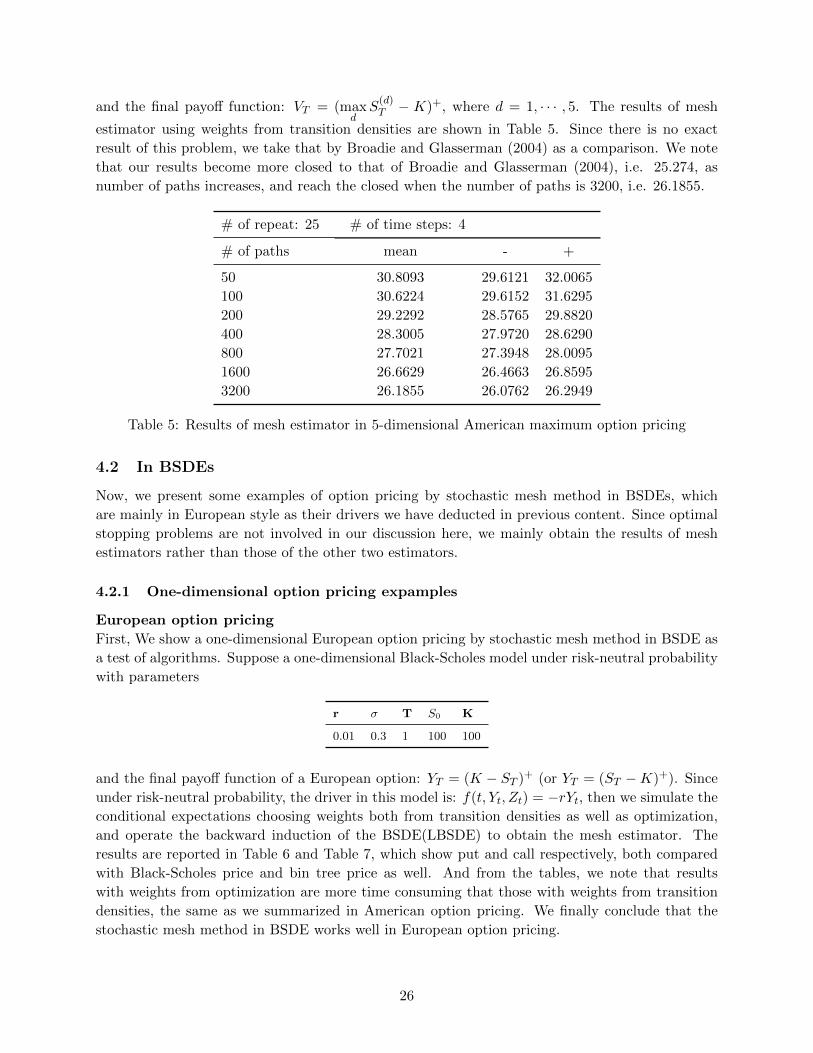
and the final payoff function: VT = (maxdS
(d)T − K)+, where d = 1, · · · , 5. The results of mesh
estimator using weights from transition densities are shown in Table 5. Since there is no exact
result of this problem, we take that by Broadie and Glasserman (2004) as a comparison. We note
that our results become more closed to that of Broadie and Glasserman (2004), i.e. 25.274, as
number of paths increases, and reach the closed when the number of paths is 3200, i.e. 26.1855.
# of repeat: 25 # of time steps: 4
# of paths mean - +
50 30.8093 29.6121 32.0065
100 30.6224 29.6152 31.6295
200 29.2292 28.5765 29.8820
400 28.3005 27.9720 28.6290
800 27.7021 27.3948 28.0095
1600 26.6629 26.4663 26.8595
3200 26.1855 26.0762 26.2949
Table 5: Results of mesh estimator in 5-dimensional American maximum option pricing
4.2 In BSDEs
Now, we present some examples of option pricing by stochastic mesh method in BSDEs, which
are mainly in European style as their drivers we have deducted in previous content. Since optimal
stopping problems are not involved in our discussion here, we mainly obtain the results of mesh
estimators rather than those of the other two estimators.
4.2.1 One-dimensional option pricing expamples
European option pricing
First, We show a one-dimensional European option pricing by stochastic mesh method in BSDE as
a test of algorithms. Suppose a one-dimensional Black-Scholes model under risk-neutral probability
with parameters
r σ T S0 K
0.01 0.3 1 100 100
and the final payoff function of a European option: YT = (K − ST )+ (or YT = (ST −K)+). Since
under risk-neutral probability, the driver in this model is: f(t, Yt, Zt) = −rYt, then we simulate the
conditional expectations choosing weights both from transition densities as well as optimization,
and operate the backward induction of the BSDE(LBSDE) to obtain the mesh estimator. The
results are reported in Table 6 and Table 7, which show put and call respectively, both compared
with Black-Scholes price and bin tree price as well. And from the tables, we note that results
with weights from optimization are more time consuming that those with weights from transition
densities, the same as we summarized in American option pricing. We finally conclude that the
stochastic mesh method in BSDE works well in European option pricing.
26

# of repeat: 250 # of time steps: 11
via transition density (966.120 s)
# of mesh mean - +
50 7.3377 7.1297 7.5456
100 7.1914 7.0514 7.3313
200 7.3183 7.225 7.4115
400 7.3239 7.2528 7.3949
800 7.3191 7.2682 7.37
1600 7.2967 7.2621 7.3313
via optimization (3269.783 s)
# of mesh mean - +
50 5.2054 4.9473 5.4635
100 6.1868 6.0345 6.3391
200 6.6665 6.5812 6.7518
400 6.909 6.854 6.9641
800 7.0696 7.0353 7.104
1600 7.0907 7.0686 7.1128
BIN. TREE EUR PUT PRICE: 7.412492924175051
BLACK-SCHOLES EUR PUT PRICE: 7.217875919378269
Table 6: Results of European put option pricing
27

# of repeat: 250 # of time steps: 11
via transition density (1008.034 s)
# of mesh mean - +
50 16.9271 16.5328 17.3214
100 16.9405 16.6713 17.2096
200 16.8508 16.6336 17.0679
400 16.7598 16.6087 16.911
800 16.8473 16.7414 16.9532
1600 16.9198 16.8453 16.9944
via optimization (3349.198 s)
# of mesh mean - +
50 15.5993 15.4091 15.7896
100 16.3935 16.2812 16.5059
200 16.4425 16.3642 16.5208
400 16.7464 16.6989 16.7939
800 16.7729 16.7387 16.807
1600 16.8104 16.7886 16.8322
BIN. TREE EUR CALL PRICE: 16.928751120579168
BLACK-SCHOLES EUR CALL PRICE: 16.734134115782318
Table 7: Results of European call option pricing
European option with different interest rates
We now consider a one dimensional Black-Scholes model with parameters
µ σ r R T S0 K
0.06 0.2 0.04 0.06 0.5 100 100
and payoff function of a European option: YT = (ST −K)+, where R and r represent the borrowing
and lending interest rates respectively. According to (3.4), the drivers of this model are:
f(t, Yt, Zt) =r − µσ
Zt − rYt + (Yt −Ztσ
)−(R− r)
=R− µσ
Zt −RYt + (Yt −Ztσ
)+(R− r).
Since it is non-linear, for the simplicity of calculation, we use the explicit way to solve it numer-
ically.25 Specifically, Y0 can be given by the Black-Scholes formula evaluated with interest rate
R.26 Then the results of mesh estimators under both drivers in (non-linear) BSDE are presented in
Table 8 and Table 9, compared with the Black-Scholes price. From the tables, we note that results
of both drivers match together.
25The same way as we use in the following content.26Gobet, E., Lemor, J.P. and Warin, X (2005). A regression-based Monte Carlo method to solve backward stochastic
differential equations. The Annals of Applied Probability .
28

# of repeat: 250 # of time steps: 6
via transition density
# of mesh mean - +
50 7.1310 6.9596 7.3023
100 7.1796 7.0611 7.2980
200 7.2116 7.1253 7.2979
400 7.1507 7.0885 7.2129
800 7.1503 7.1067 7.1939
1600 7.1501 7.1189 7.1812
via optimization
# of mesh mean - +
50 7.1755 7.1542 7.1969
100 7.1508 7.1376 7.1640
200 7.1791 7.1695 7.1887
400 7.1759 7.1696 7.1822
800 7.1806 7.1755 7.1856
1600 7.1824 7.1788 7.1860
BLACK-SCHOLES EUR CALL PRICE( with R): 7.15
Table 8: Results of European call option pricing with different interest rates under 1st driver
29

# of repeat: 250 # of time steps: 6
via transition density
# of mesh mean - +
50 7.1334 6.9562 7.3106
100 7.0978 6.9638 7.2318
200 7.1921 7.1087 7.2756
400 7.1212 7.0607 7.1816
800 7.1858 7.1446 7.2271
1600 7.1360 7.1053 7.1667
via optimization
# of mesh mean - +
50 7.1813 7.1605 7.2021
100 7.1577 7.1441 7.1713
200 7.1617 7.1518 7.1716
400 7.1811 7.1751 7.1871
800 7.1730 7.1680 7.1779
1600 7.1807 7.1773 7.1840
BLACK-SCHOLES EUR CALL PRICE( with R): 7.15
Table 9: Results of European call option pricing with different interest rates under 2nd driver
European combination with different interest rates
We again consider a one dimensional Black-Scholes model with parameters
µ σ r R T S0 K1 K2
0.05 0.2 0.01 0.06 0.25 100 95 105
and payoff function of a European option: YT = (ST − K1)+ − 2(ST − K2)+, where K1 and K2
are the strike prices, R and r represent the borrowing and lending interest rates respectively. The
drivers of the model are the same as those in prior example. Then the results of mesh estimators
under the 1st driver in (Non-Linear) BSDE are shown in Table 10, compared with the estimated
Black-Scholes price by Gobet et al. (2005).
30

# of repeat: 250 # of time steps: 6
via transition density
# of mesh mean - +
50 2.9568 2.8809 3.0327
100 2.9158 2.8618 2.9699
200 2.9035 2.8671 2.9399
400 2.9185 2.8940 2.9431
800 2.9192 2.9007 2.9377
1600 2.9245 2.9101 2.9388
via optimization
# of mesh mean - +
50 2.6433 2.5733 2.7134
100 2.8161 2.7767 2.8554
200 2.9051 2.8819 2.9283
400 2.9308 2.9137 2.9478
800 2.9524 2.9399 2.9649
1600 2.9644 2.9563 2.9726
ESTIMATED BS PRICE: 2.95
Table 10: Results of European call combination option pricing with different interest rates
4.2.2 Geometric average of multiple underlying assets
Next, we give an example of multi-dimensional case. Here we consider a European geometric average
call option on 7 independent assets, of which each is identically modeled as the same geometric
Brownian motion with parameters
r σ δ T D S0 K
0.03 0.4 0.05 1 7 100 100
and payoff function: YT = (7
√∏7d=1 S
(d)T −K)+. The driver of this model is also: f(t, Yt, Zt) = −rYt,
and the weights are chosen only from transition densities. Since the Brownian motion generated in
this example is 7-dimensional, which is actually formed by 7 independent one-dimensional Brownian
motions, then we take the average of them in our calculation of mesh estimator. The results are
presented in Table 11. As known in previous American geometric average option pricing, this
problem can be reduced to a single dimension one, where binomial tree method provides us an
accurate value27, i.e. 2.419.
27Broadie, M. and Glasserman P. (2004). A stochastic mesh method for pricing high-dimensional American options.
Journal of Computational Finance.
31

# of repeat: 25 S0 = 100
# of time steps: 4 (284.054 s) # of time steps: 6 (418.238 s) # of time steps: 8 (546.969 s)
# of paths mean - + mean - + mean - +
50 2.4659 2.0373 2.8944 2.4405 2.1534 2.7277 2.3497 2.0675 2.6319
100 2.3657 2.1851 2.5463 2.5171 2.2687 2.7655 2.3124 2.0424 2.5823
200 2.3718 2.2065 2.5370 2.3612 2.2302 2.4923 2.2760 2.1263 2.4258
400 2.4391 2.3117 2.5665 2.3713 2.2361 2.5065 2.4418 2.2958 2.5877
800 2.3671 2.2634 2.4709 2.3973 2.3081 2.4866 2.4571 2.3738 2.5405
1600 2.4460 2.3884 2.5035 2.3986 2.3369 2.4603 2.4191 2.3649 2.4734
BIN. TREE EUR CALL PRICE: 2.419
Table 11: Results of mesh estimator in 7-dimensional European geometric average option pricing
From the table, we note that in this example of European geometric average option pricing,
we succeed to avoid the disturbance of the number of time steps to our results, which happens in
previous American case. Besides, the time consumption is nearly linear with respect to the number
of time steps as well. Moreover, the accuracy here is also acceptable.
4.2.3 Maximum of multiple underlying assets
Similarly, we consider a European maximum call option on 5 independent underling assets, of which
each is identically modeled as geometric Brownian motion with parameters
r σ δ T D S0 K
0.05 0.2 0.1 3 5 100 100
and the final payoff function: YT = (maxdS
(d)T −K)+, where d = 1, · · · , 5. The driver of the model
is the same as prior one. This kind of option is priced by Johnson (1987), and we take the results
by Broadie and Glasserman (2004) as a comparison. The results of mesh estimator using weights
from transition densities are shown in Table 12.
# of repeat: 25 # of time steps: 4
# of paths mean - +
50 23.8665 22.6327 25.1003
100 25.0915 24.0018 26.1811
200 24.5982 23.8875 25.3088
400 24.2702 23.8931 24.6472
800 24.2186 23.8358 24.6014
1600 24.3495 24.1261 24.5729
3200 24.4619 24.3043 24.6194
B&G EUR CALL PRICE: 23.052
Table 12: Results of mesh estimator in 5-dimensional European maximum option pricing I
As mentioned in our previous discussion, the number of time steps n does not represent the
exercise dates but the number of times we operate the calculation of recursion of BSDE, so n = 4
32

might be too small to provide us accurate results, then the results of n = 8 with the same other
parameters are shown in Table 13, which are indeed more accurate.
# of repeat: 25 # of time steps: 8
# of paths mean - +
50 23.0482 21.7225 24.3739
100 23.6059 22.4657 24.7460
200 23.2390 22.4541 24.0240
400 23.9167 23.2676 24.5657
800 23.6582 23.3076 24.0088
1600 23.6666 23.4124 23.9208
3200 23.5832 23.4323 23.7340
B&G EUR CALL PRICE: 23.052
Table 13: Results of mesh estimator in 5-dimensional European maximum option pricing II
4.2.4 Some more examples
Now, we present several problems that can hardly been solved by other methods but can be dealt
with easily by applying stochastic mesh method to BSDEs.
Geometric average of multiple underlying assets with different interest rates
There is an example, which combines European call option with different interest rates and
geometric average of 7 independent underlying assets. Suppose each of the assets is identically
modeled by geometric Brownian motion with parameters
µ σ r R T D S0 K
0.06 0.2 0.04 0.06 0.5 7 100 100
and the final payoff function: YT = (7
√∏7d=1 S
(d)T −K)+, where R and r represent the borrowing
and lending interest rates respectively. From above, here we take the first driver of this model:
f(t, Yt, Zt) =r − µσ
Zt − rYt + (Yt −Ztσ
)−(R− r).
The results of mesh estimators using weights from transition densities in (non-linear) BSDE are
presented in Table 14.
33

# of repeat: 25 # of time steps: 6
# of paths mean - +
50 2.6725 2.4672 2.8779
100 2.5765 2.4581 2.6950
200 2.6629 2.5928 2.7330
400 2.7300 2.6693 2.7908
800 2.7053 2.6609 2.7497
1600 2.7184 2.6787 2.7580
Table 14: Results of 7-dimensional European geo-average option pricing with different interest rates
Maximum of multiple underlying assets with different interest rates
Similarly, we consider a European maximum call option with different interest rates on 5 in-
dependent underlying assets, of which each is identically modeled as geometric Brownian motion
with parameters
µ σ r R T D S0 K
0.06 0.2 0.04 0.06 0.5 5 100 100
and the final payoff function: YT = (maxdS
(d)T −K)+, where d = 1, · · · , 5, R and r represent the
borrowing and lending interest rates respectively. The driver of the model is the same as that
in prior example. Then the results of mesh estimators using weights from transition densities in
(non-linear) BSDE are presented in Table 15.
# of repeat: 25 # of time steps: 6
# of paths mean - +
50 19.3563 18.8002 19.9123
100 19.1840 18.6900 19.6780
200 19.6158 19.3000 19.9316
400 19.4089 19.2242 19.5937
800 19.2094 19.0375 19.3813
1600 19.2389 19.1526 19.3252
Table 15: Results of 5-dimensional European maximum option pricing with different interest rates
Geometric average combination of multiple underlying assets with different interest
rates
Finally, we consider a European geometric average call combination option on 7 independent
underlying assets, of which each is identically modeled as geometric Brownian motion with param-
eters
µ σ r R T D S0 K1 K2
0.05 0.2 0.01 0.06 0.25 7 100 95 105
34

and payoff function of a European option: YT = (7
√∏7d=1 S
(d)T − K1)+ − 2(
7
√∏7d=1 S
(d)T − K2)+,
where K1 and K2 are the strike prices, R and r represent the borrowing and lending interest rates
respectively. The driver of the model is also the same as prior one. Then the results of mesh
estimators in (non-linear) BSDE are shown in Table 16.
# of repeat: 25 # of time steps: 6
# of paths mean - +
50 4.8434 4.6878 4.9990
100 4.7504 4.6432 4.8576
200 4.6789 4.5952 4.7627
400 4.7198 4.6541 4.7855
800 4.6977 4.6648 4.7307
1600 4.6819 4.6569 4.7069
Table 16: Results of 7-d European geo-ave combination option pricing with different interest rates
ConclusionIn this dissertation we show the application of stochastic mesh method in BSDEs. We review the
origin of this method, which is developed for pricing American option. We introduce the BSDEs
and detail the process of deduction of drivers and recursion in BSDEs, where we finally apply
stochastic mesh method. Numerical results are also included to illustrate the performance of the
method in BSDEs of some examples, particularly, in derivative pricing. Although we are mainly
concerned with the European option problem, we can still go a bit further in future research for
the other types of option pricing to check the availability of this method in BSDEs, for example,
the American option pricing in reflected BSDEs as mentioned, of which we can obtain the results
directly by stochastic mesh method as well. Besides, there are a lot more fields we can apply
our method as long as we can solve the BSDEs, for instance, in complete markets, the Follmer-
Schweizer strategy is just given by the solution of a BSDE. Even on the efforts of previous research,
there are still quite a few parts that can be improved in the method. One possible way suggested
by Broadie is that we might try to reduce the connection between the node j at time step i and
all the nodes at time step i + 1 to that between the node j at time step i and some fixed (not
all) nodes at time step i + 1. This is remarkable, since it reduce the calculation effort quadratic
to the number of nodes at each time step into linear, but the definition of the weights need to be
concerned nevertheless.
35

References
Avramidis, A. N. and Hyden, P. (1999). Efficiency improvements for pricing American options
with a stochastic mesh. Proceedings of the 31st conference on Winter simulation: Simulation — a
bridge to the future 1, 344-350.
Avramidis, A. N. and Hyden, P. (1999). Efficient Simulation Techniques for Pricing American
Option. Unpublished manuscript.
Avramidis, A. N. and Matzinger H. (2004). Convergence of the stochastic mesh estimator for pric-
ing Bermudan options. Journal of Computational Finance 7(2), 73-91.
Bally, V. (1997). Approximation scheme for solutions of BSDE. Pitman Research Notes in Mathe-
matics Series 364, 177-191.
Bally, V. and Pages, G. (2003). A quantization algorithm for solving multidimensional discrete-
time optimal stopping problems. Bermoulli 9, 1003-1049.
Bally, V., Pages, G. and Printems, J. (2001). A stochastic quantization method for nonlinear prob-
lems. Monte Carlo Methods and Applications 7(1-2), 21-34.
Bismut, J.M. (1973). Conjugate Convex Functions in Optimal Stochastic Control. Journal of
Mathematical Analysis and Applications 44, 384-404.
Black, F. and Scholes, M. (1973). The pricing of options and corporate liabilities. Journal of
Political Economy 81, 637-654.
Bouchard, B. and Touzi, N. (2004). Discrete time approximation and Monte Carlo simulation of
backward stochastic differential equations. Stochastic Processes and their Applications 111, 175-
206.
Broadie, M. and Glasserman P. (1997). Pricing Amrican-style securities by simulation. Journal of
Economic Dynamics and Control 21, 1323-1352.
Broadie, M. and Glasserman P. (2004). A stochastic mesh method for pricing high-dimensional
American options. Journal of Computational Finance 7(4), 35-72.
Broadie, M., Glasserman P. and Ha, Z. (2000). Pricing American options by simulation using a
stochastic mesh with optimized weights. Probabilistic Constrained Optimization, 32-50.
Broadie, M. and Yamamoto, Y (2003). Application of the fast Gauss transform to option pricing.
Management Science 49(8), 1071-1088.
El Karoui, N., Peng, S. and Quenez, M.C. (1997). Backward Stochastic Differential Equations in
Finance. Mathematical Finance 7, 1-71.
36

El Karoui, N., Hamadene, S. and Matoussi, A. (2008). Backward stochastic differential equations
and applications. Springer 27, 267-320.
Follmer, H. and Schweizer, M. (1990). Hedging of contingent claims under incomplete information.
Applied Stochastic Analysis 5, 389-414.
Glasserman, P. (2004). Monte Carlo Methods in Financial Engineering. Springer.
Gobet, E., Lemor, J.P. and Warin, X (2005). A regression-based Monte Carlo method to solve
backward stochastic differential equations. The Annals of Applied Probability 15(3), 2172-2202.
Johnson, H. (1987). Options on the maximum or the minimum of several assets. Journal of Fi-
nancial and Quantitative Analysis 22(3), 277-283.
Ma, J., Protter, P. and Yong, J.M. (1994). Solving forward-backward stochastic differential equa-
tions explicitly – A four step scheme. Probability Theory Related Fields 98, 339-359.
Merton, R. (1973). Theory of Rational Option Pricing. Bell Journal of Economics and Manage-
ment Science 4, 141-183.
Merton, R. (1991). Continuous Time Finance. Basil Blackwell.
Pardoux, E. and Peng, S. (1990). Adapted Solution of a Backward Stochastic Differential Equation.
Systems & Control Letters 14, 55-61.
Pardoux, E. and Peng, S. (1992). Backward Stochastic Differential Equations and Quasilinear
Parabolic Partial Differential Equations. Lecture Notes in CIS 176, 200-217.
Peng, S. (2003). Dynamically consistent evaluations and expectations. Technical report, Institute
Mathematics, Shandong University.
Peng, Y., Gong, B., Liu, H. and Zhang, Y. (2010). Parallel computing for option pricing based
on the backward stochastic differential equation. High Performance Computing and Applications,
325-330.
37