the application of variable speed limits to arterial roads
TRANSCRIPT

University of Southern Queensland
The Application of Variable Speed Limits to
Arterial Roads for Improved Traffic Flow
A dissertation submitted by
Hamdi Abdulkareem Mohammed Al-Nuaimi
B.Sc. Eng., M.Sc. Eng.
For the award of
Doctor of Philosophy
2014


i
ABSTRACT
Traffic congestion problems continue to increase in large cities due to rapidly
increasing travel demand and a lack of transport infrastructure. Congestion causes
mobility and efficiency loss, safety reduction, increased fuel consumption and
excessive air pollution. A number of traffic management strategies have been
proposed and some are applied in cities, such as diverting traffic from peak periods
to off-peak periods using congestion pricing, reduced speed limits, coordinated
traffic signals along major arterial roads, or adding additional lanes where network
expansion is feasible. Among the many solutions to traffic congestion, operational
treatments for existing road networks provide more cost efficient traffic operation
due to their relatively low cost. This research looks to improve efficiency through the
application of Variable Speed Limits (VSLs). While VSLs have been used to
improve traffic conditions on congested motorways in terms of mobility, safety and
travel time, they are largely untested on signalized urban arterial roads.
Griffith Arterial Road (GAR) U20 was selected as the case study for the
research. GAR is part of the Brisbane Urban Corridor (BUC), and is approximately
11.5 km long and lies between the Gateway Motorway and the Ipswich Motorway.
The average daily traffic volume (ADT) is between 18,000 vehicles to 24,000
vehicles. The number of lanes at approaches to signalised intersection varies from 1
to 4.
In the context of this research, the study used STREAMS data and real world
data collected using six high definition (HD) video cameras to develop a VISSIM
model and to discern the effectiveness of applying VSL control. VISSIM is a time
step and a psycho-physical car following model developed to model urban traffic and
public transit operations. The VISSIM model was extensively calibrated and
validated with the empirical data collected regarding measure of effectiveness such
as traffic volumes, volume distribution, and saturated headway along the west bound
(WB) and eastbound (EB) directions. The simulated model allowed the testing of
different control strategies for VSL and Integrated Traffic Control System (ITCS)
under different scenarios and circumstances. It helped to contrast the traffic flow
parameters of invariant (no controlled speed) and VSL (controlled speed) conditions.
Multiple simulation runs were considered in the calibration and evaluation process.
The measures of effectiveness used to characterise the operational quality of
signalized intersections were delay, queue length, and number of stops. In addition,
flow, speed and density parameters were used to characterise the changes in traffic
performance for the arterial road.
This thesis investigates the application of VSLs for control of upstream traffic as a
proposed traffic control strategy on the GAR. The objective was to investigate how
dynamic VSL and signal control systems could be used in an integrated approach to
traffic management to improve the traffic efficiency, safety, and mobility of a
congested urban arterial road. The research indicates that the application of VSL
could improve the traffic performance and safety during the peak period. It helped to
maintain a planned continuous flow through coordinated intersections to avoid
congestion. Integrating VSL with other traffic congestion management (changing the
signal timings for the congested traffic) appeared effective in improving traffic
conditions and reducing total travel time on the GAR. The research highlighted some
important elements that could be used for the design and implementation of VSL
systems using intelligent transport systems.

ii

iii
Certification of Dissertation
I certify that the thoughts, experimental work, numerical outcomes and conclusions
reported in this dissertation are entirely my own efforts, except where otherwise
acknowledged. To the best of my knowledge, I also certify that the work presented in
this thesis is original, except where due references are made.
…………………………………….
/ / 2014
Signature of Candidature
Hamdi Abdulkareem Mohammed
Date
ENDORSEMENT
……………………………………
/ / 2014
Signature of Supervisor
Prof. Ron Ayers
Date
…………………………………...
/ / 2014
Signature of Supervisor
Prof. Frank Bullen Date
…………………………………….
/ / 2014
Signature of Supervisor
Dr. Kathirgamalingam Somasundaraswaran
Date


v
Acknowledgments
I would like to express my sincere gratefulness to Prof. Ron Ayers, my principal
supervisor, for his guidance, encouragement, persistence, patience and expert advice.
I would also like to thank my associated supervisor Prof. Frank Bullen for his expert
advice and valuable input to my research. It is my luck and great honour to be their
student. Without their guidance, I would not be able to complete this research. Also,
I am very thankful to my associated supervisor Dr. Kathirgamalingam, who provided
me with invaluable help and support.
I owe my deepest gratitude to the spirit of my father, who always in my heart and
dreams and to my mother, who without her pray, I wouldn’t reach this stage.
My admiration and respect go to my wonderful wife, Enas, who without her
support and encouragement I could not be able to finish my study. My thanks go to
my smart son, Diyar, to my beautiful daughter, Dima, to my little gorgeous
daughters Diane and Dania for their encouragement, patience and endless love
during my PhD study.
Many thanks go to my brothers, sisters and relatives for their inspiration and pray.
Great thanks and attitudes go to my brother, Husham Al-Nuaimi, for his infinite
support and encouragement during all the period of my life.
I would like to extend my thanks to the University of Southern Queensland (USQ)
and special thanks to Faculty of Civil Engineering and Surveying for their support
throughout my academic studies. I would also like to acknowledge all the staff
members of PTV vision in Brisbane and especially Dr. Julian Laufer and Dr. Mamun
Rahman for their cooperation and support during the course of this research.
Furthermore, great thanks go to the Department of Transport and Main Roads in
Queensland for their help in providing and collecting traffic data for the Griffith
Arterial Road.
I wish to express my sincerest gratitude to my sponsor Iraqi Government, and
special thanks go to the Iraqi Cultural Attaché in Canberra for providing the funding
required fulfilling this thesis during the period of the research. I wish to thank all
Iraqi friends and colleagues I have met, who have helped to provide encouragement,
guidance or made my life in Toowoomba an enjoyable experience.


vii
Associated Publication
Al-Nuaimi, H, Ayers, R & Somasundaraswaran, K (2013), ‘Modelling interrupted
flow conditions on an arterial road using VISSIM software’, proceeding paper
presented to 14th Road Engineering Association of Asia and Australasia Conference
(REAAA 2013): The Road Factor in Economic Transformation, 26-28 Mar 2013,
Kuala Lumpur, Malaysia.
Al-Nuaimi, H, Ayers, R & Somasundaraswaran, K (2012), ‘The effectiveness of
using variable speed limit on the performance of an interrupted flow’, proceeding
paper presented to IASTED International Conference on Engineering and Applied
Science (EAS 2012): Applications for the 21st Century, 27-29 Dec 2012, Colombo,
Sri Lanka.

viii

ix
Table of Content
List of Figures xiii
List of Tables xvii
List of Abbreviations xix
Chapter 1 Introduction
1.1 Background 1
1.2 Objectives of the study 1
1.3 Significance of the study 2
1.4 Study methodology 3
1.5 Thesis layout 4
Chapter 2 Literature Review
2.1 Introduction 5
2.2 The performance of signalised intersections 7
2.2.1 Delay 7
2.2.2 Vehicle queuing 10
2.2.3 Number of stops 13
2.3 Traffic control management strategies 15
2.3.1 Road pricing strategies 15
2.3.2 Constraint traffic flow strategy 17
2.3.3 Metering flow strategies 21
2.3.4 Variable speed limit Strategy (VSL) 25
2.4 The implementation of VSL on arterials 28
2.4.1 Coordination traffic system with no queued vehicles 28
2.4.2 Coordination traffic system with queued vehicles exist 29
2.4.3 Coordination traffic system with spill back exist 31
2.4.4 VSL and the performance of signalised intersection 33
2.4.5 VSL use when the queued vehicles consume the entire green interval 34
2.4.6 Applying VSL under spill back conditions 35
2.4.7 Using VSLs in urban areas 37
2.4.8 Mathematical approach of VSLs in urban areas 38
2.5 Summary 40
Chapter 3 Survey & Data Collection
3.1 Introduction 41
3.2 Selection of study area 42
3.3 Data Collection 45
3.3.1 QDTMR database 45

x
3.3.2 Field data 50
3.3.3 Field data processing 52
3.4 Floating car test 65
3.5 Summary 67
Chapter 4 Modelling the Griffith Arterial Road using VISSIM software
4.1 Introduction 69
4.2 VISSIM an overview 69
4.3 Development of VISSIM modelling 72
4.3.1 Physical road network & traffic signal timing 72
4.3.2 Coding traffic Data 72
4.3.3 Driving behaviour 72
4.4 Calibration and validation processes 72
4.4.1 VISSIM calibration 72
4.4.2 Validation criteria 75
4.5 Calibration and validation implications 76
4.5.1 Calibration results of mainstream flow 76
4.5.2 The variability of simulated flow at peak hour 78
4.5.3 Calibration results of flow distribution 79
4.5.4 Calibration results of saturated headway 81
4.6 Summary 83
Chapter 5 Description of Local Traffic Situation at Griffith Arterial Road
5.1 Introduction 85
5.2 The study site 85
5.3 Traffic flow description 86
5.3.1 Description of traffic flow in WB direction 86
5.3.2 Description of traffic flow in EB direction 95
5.4 Summary 105
Chapter 6 Evaluation of VSL Application to the Griffith Arterial Road
6.1 Introduction 107
6.2 Speed Limits management 107
6.3 Evaluation of Scenario 1 on the performance of intersection 2 109
6.3.1 Evaluation of average queue length 109
6.3.2 Evaluation of average delay parameter 110
6.3.3 Evaluation of average stopped delay 114
6.3.4 Evaluation of average number of stops 115
6.4 Evaluation of Scenario 1 on the performance of the congested link 117
6.4.1 Evaluation of average traffic flow 117
6.4.2 Evaluation of average speed 118

xi
6.4.3 Evaluation of average density 122
6.5 Evaluation of Scenario 2 on the performance of intersection 2 123
6.5.1 The influence of Scenario 2 on the intersection parameters 123
6.5.2 Evaluation of Scenario 2 on the performance of the congested link 126
6.6 Evaluation of Scenario 3 on the performance of intersection 2 129
6.6.1 The influence of Scenario 3 on the intersection parameters 129
6.6.2 Evaluation of Scenario 3 on the performance of the congested link 132
6.7 Evaluation of Scenario 4 on the performance of intersection 2 135
6.7.1 The influence of Scenario 4 on the intersection parameters 135
6.7.2 Evaluation of Scenario 4 on the performance of the congested link 138
6.8 Comparison and optimisation of VSL scenarios 141
6.8.1 Evaluation of effectiveness of VSL at busy Intersection 141
6.8.2 Evaluation of effectiveness of VSL on busy link 143
6.9 The influence of VSLs optimisation on the total travel time 145
6.10 Summary 146
Chapter 7 Evaluation of Signalised / VSL Integrated Traffic Control System
7.1 Introduction 149
7.2 Traffic scenario descriptions 149
7.2.1 Traffic Scenario 1 (ITCS 1) 149
7.2.2 Traffic Scenario 2 (ITCS 2) 150
7.3 The aim of ITCS 151
7.4 Evaluation procedure of ITCS 151
7.5 Results and discussions 152
7.5.1 Effect of ITCS 1 on the performance of Intersection 2 152
7.5.2 Evaluation of ITCS1 on the performance of macroscopic traffic flow
parameters 161
7.5.3 Evaluation of ITCS 2 on the performance of intersection 2 169
7.5.4 Evaluation of ITCS 2 on the performance of traffic flow parameters 179
7.6 Comparison of VSL applications and ITCS scenarios 187
7.7 Influence of ITCS on total travel time 191
7.8 Summary 192
Chapter 8 Summary and Conclusion
8.1 Main conclusions from this study 195
8.1.1 The impact of VSL and ITCS on intersection parameters 195
8.1.2 The impact of VSL and ITCS on macroscopic traffic characteristics 195
8.1.3 The impact of VSL and ITCS on TTT 196
8.2 The impact of VSL and ITCS on annual savings 196
8.3 Summary 197
8.4 Recommendations for future work 198

xii
References 199
Appendix A
A.1 Development of VISSIM modelling 209
A.1.1 Physical road network & traffic signal timing 209
A.1.2 Coding traffic data 211
A.1.3 Driving behaviour 213
A.2 Calibration process 217
A.2.1 Identification of the measure of effectiveness (MOE) 217
A.2.2 Initial iteration run 218
A.2.3 Error messages 218
A.2.4 Visual evaluation 219
A.2.5 Determination of the minimum number of runs 220
Appendix B Evaluation of VSL Applications on Intersection 6
B.1 Preface 225
B.2 VSL control management 225
B.3 Evaluation of scenario 1 227
B.3.1 Evaluation of intersection parameters 227
B.3.2 Evaluation of macroscopic traffic characteristics 230
B.4 Evaluation of Scenario 2 233
B.4.1 Evaluation of intersection parameters 233
B.4.2 Evaluation of macroscopic traffic characteristics 236
B.5 Evaluation of Scenario 3 239
B.5.1 Evaluation of intersection parameters 239
B.5.2 Evaluation of macroscopic traffic characteristics 234
B.6 Evaluation of Scenario 4 245
B.6.1 Evaluation of intersection parameters 245
B.6.2 Evaluation of macroscopic traffic characteristics 249
B.7 Comparison and optimisation of VSL scenarios 251
B.8 Evaluation of total travel time 252

xiii
List of Figures
Chapter 1 Figure title Page
Figure 1.1 Schematic illustration showing the scope of the current research 3
Figure 1.2 Study methodology 4
Chapter 2 Figure title Page
Figure 2.1 Delay components, Source: (TRB, 2000) 8
Figure 2.2 Traffic entering the restricted zone under electronic road pricing 16
Figure 2.3 Traffic entering the restricted zone under ERP, (1998) 17
Figure 2.4 The shape of MFD 20
Figure 2.5 Average vehicle travel time for different control modes 21
Figure 2.6 A general traffic network 22
Figure 2.7 Two cases: (a) without ramp metering control and (b) with ramp
metering control; grey areas indicate congestion zones 23
Figure 2.8 Spatial equity and mobility on Trunk Highway 169 24
Figure 2.9 Flow-density diagram versus VSLs. Where b=1, 0.8 and 0.6 26
Figure 2.10 (a) Potential VSL impact on under-critical mean speeds and (b) cross-
point of diagrams with and without VSL 27
Figure 2.11 Ideal offset 28
Figure 2.12 The effect of speed on the traffic operation 29
Figure 2.13 The effect of queued vehicles on the offset calculation 30
Figure 2.14 The operation of traffic flow under using normal offset 32
Figure 2.15 Equity offset process 32
Figure 2.16 VSL plan 33
Figure 2.17 Offset operation pre-speed limit initiation 34
Figure 2.18 Arrival flow under post- speed limit control 35
Figure 2.19 Schematic of using new spill back management 36
Figure 2.20 Bottleneck activation view of roadway without using VSLs 37
Figure 2.21 Schematic view of roadway traffic flow control using VSLs 37
Figure 2.22 Schematic view of traffic flow details 38
Figure 2.23 VSLs control algorithm 40
Chapter 3 Figure title Page
Figure 3.1 Survey design 42
Figure 3.2 U20 Griffith Arterial Road, Brisbane, Queensland (QLD), Australia 43
Figure 3.3 Study area layout 44
Figure 3.4 ADT for EB arterial links 46
Figure 3.5 Variation in traffic volumes at the EB direction 47
Figure 3.6 Variation in traffic volumes at the WB direction 47
Figure 3.7 Video camera locations 51
Figure 3.8 Snapshot photo for intersection 1 52
Figure 3.9 Virtual Dub snapshot for intersection 2 53
Figure 3.10 Traffic distribution at intersection 1 54
Figure 3.11 Variation of HV for intersection 1 55
Figure 3.12 Traffic variations at intersection 2 55
Figure 3.13 Variation of HV at intersection 2 56
Figure 3.14 Traffic variations at intersection 3 56
Figure 3.15 Variation of HV at intersection 3 57
Figure 3.16 Traffic variations at intersection 4 57
Figure 3.17 Variation of HV at intersection 4 58
Figure 3.18 Traffic variations at intersection 5 58
Figure 3.19 Variation of HV at intersection 5 59
Figure 3.20 Traffic variations at intersection 6 59

xiv
Figure 3.21 Variation of HV at intersection 6 60
Figure 3.22 Saturated headway at EB of intersection 2, first trial 61
Figure 3.23 Saturated headway at EB of intersection 2, second trial 61
Figure 3.24 Saturated headway at EB of intersection 2, first trial 62
Figure 3.25 Saturated headway at EB of intersection 2, second trial 62
Figure 3.26 Saturated headway at WB of intersection 2, first trial 62
Figure 3.27 Saturated headway at WB of intersection 2, second trial 63
Figure 3.28 Schematic of signal phases 65
Chapter 4 Figure title Page
Figure 4.1 Car following model by Wiedemann: Source PTV 2011 70
Figure 4.2 Calibration process 73
Figure 4.3 Coefficient of variation of simulated flow under high traffic volumes 79
Figure 4.4 Coefficient of variation of simulated flow versus field flow 79
Figure 4.5 Comparison of saturated headway for EB/TH 82
Figure 4.6 Comparison of saturated headway for EB/RT 82
Figure 4.7 Comparison of saturated headway for WB/TH 83
Chapter 5 Figure title Page
Figure 5.1 Study site 86
Figure 5.2 Speed-flow relationship for WB link of intersection 1 87
Figure 5.3 Speed variation for various survey days of STREAMS data 89
Figure 5.4 Speed-flow relationship for WB link at intersection 2 90
Figure 5.5 Speed variations for WB link at Intersection 2 92
Figure 5.6 Speed-flow relationship for WB link at intersection 3 93
Figure 5.7 Speed variations for the WB link at Intersection 3 94
Figure 5.8 Speed-flow relationships for the EB link at intersection 6 96
Figure 5.9 Speed variations for the EB link at Intersection 6 97
Figure 5.10 Speed-flow relationships for the EB link at intersection 5 98
Figure 5.11 Speed variations for the EB link at Intersection 5 100
Figure 5.12 Speed-flow relationships for the EB link at intersection 4 101
Figure 5.13 Speed variations for the EB link at Intersection 4 102
Figure 5.14 Speed-flow relationships for the EB link at intersection 3 104
Figure 5.15 Speed variations for the EB link at Intersection 3 105
Figure 5.16 Speed distributions in the WB and EB direction 106
Chapter 6 Figure title Page
Figure 6.1 Locations of controlled speed in the WB direction 108
Figure 6.2 Average queue length for Scenario 1 110
Figure 6.3 The efficiency of Scenario 1 on the average queue length 110
Figure 6.4 The trend of delay under applying scenario 1 111
Figure 6.5 Efficiency of scenario 1 on delay indicators 112
Figure 6.6 Annual time savings due to Scenario 1, VSL 113
Figure 6.7 The impact of scenario 1 on the average stopped delay 114
Figure 6.8 The efficiency of scenario 1 on stoped delay indicators 115
Figure 6.9 The application of scenario 1versus average number of stops 116
Figure 6.10 The efficiency of scenario 1 on the number of stops 116
Figure 6.11 Annual savings due to reduced rear-end collisions by Scenario 1, VSL 117
Figure 6.12 Link throughput before and after VSL application 118
Figure 6.13 The efficiency of scenario 1 on the throughput of the congested link 118
Figure 6.14 Average speed before and after VSL application 119
Figure 6.15 The efficiency of Scenario 1 on average speeds 119
Figure 6.16 Traffic density before and after VSLs application 122
Figure 6.17 The efficiency of Scenario 1 on the traffic density 122
Figure 6.18 The simulation of Scenario 2 along the WB direction of the main road 124

xv
Figure 6.19 The efficiency of scenario 2 on the signalised intersection
characteristics 126
Figure 6.20 The effect of Scenario 2 on the characteristics of congested link 127
Figure 6.21 The efficiency of Scenario 2 in terms of traffic macroscopic aspect 128
Figure 6.22 The parameters of signalised intersection 2 before and after Scenario 3 130
Figure 6.23 The efficiency of Scenario 3 on the signalised parameters 132
Figure 6.24 The macroscopic characteristics before/after the application of
Scenario 3 133
Figure 6.25 The efficiency of Scenario 3 on the characteristics of congested link 134
Figure 6.26 Signalised intersection parameters under application of Scenario 4 136
Figure 6.27 The efficiency of Scenario 4 on the performance of intersection 2 138
Figure 6.28 The application of Scenario 4 on the link traffic characteristics 139
Figure 6.29 The efficiency of Scenario 4 on the link traffic parameters 141
Figure 6.30 Optimum efficiency of traffic scenarios regarding the intersection
characteristics 142
Figure 6.31 Annual delay time cost before and after applying VSL scenarios 143
Figure 6.32 Optimum efficiency of traffic scenarios regarding the link
characteristics 144
Figure 6.33 Annual vehicle accessibility after applying VSL scenarios 145
Figure 6.34 TTT comparison under control/non-control condition 145
Chapter 7 Figure title Page
Figure 7.1 Flow chart for traffic Scenario 1 (ITCS1) 150
Figure 7.2 Flow chart for traffic Scenario 2 (ITCS2) 151
Figure 7.3 Average queue length before and after applying ITCS1, SCL (a) 152
Figure 7.4 Average queue length before and after applying ITCS1, SCL (b) 153
Figure 7.5 Efficiency of ITCS 1, SCL (a) on average queue length 154
Figure 7.6 Efficiency of ITCS 1, SCL (b) on average queue length 154
Figure 7.7 Average delay before and after applying ITCS 1, SCL (a) 155
Figure 7.8 Average delay before and after applying ITCS 1, SCL (b) 155
Figure 7.9 Efficiency of ITCS 1, SCL (a) on average delay 156
Figure 7.10 Efficiency of ITCS 1, SCL (b) on average delay 156
Figure 7.11 Average stopped delay before and after applying Scenario1, SCL (a) 157
Figure 7.12 Average stopped delay before and after applying ITCS 1, SCL (b) 158
Figure 7.13 Efficiency of ITCS 1, SCL (a) on average stopped delay 158
Figure 7.14 Efficiency of ITCS 1, SCL (b) on average stopped delay 159
Figure 7.15 Average number of stops before and after applying Scenario1, SCL (a) 159
Figure 7.16 Average number of stops before and after applying Scenario1, SCL
(b) 160
Figure 7.17 Efficiency of ITCS 1, SCL (a) on average number of stops 160
Figure 7.18 Efficiency of ITCS 1, SCL (b) on average number of stops 161
Figure 7.19 Average speed before and after applying Scenario1, SCL (a) 162
Figure 7.20 Average speed before and after applying Scenario1, SCL (b) 162
Figure 7.21 Efficiency of ITCS 1, SCL (a) on average speed 163
Figure 7.22 Efficiency of ITCS 1, SCL (b) on average speed 163
Figure 7.23 Average flow before and after applying Scenario1, SCL (a) 165
Figure 7.24 Average flow before and after applying Scenario1, SCL (b) 166
Figure 7.25 Efficiency of ITCS 1, SCL (a) on average flow 166
Figure 7.26 Efficiency of ITCS 1, SCL (b) on average flow 167
Figure 7.27 Annual vehicle accessibility after activating CS1 at SCL (b), ITCS1 167
Figure 7.28 Average density before and after applying Scenario1, SCL (a) 168
Figure 7.29 Average density before and after applying Scenario1, SCL (b) 168
Figure 7.30 Efficiency of ITCS 1, SCL (a) on average density 169
Figure 7.31 Efficiency of ITCS 1, SCL (b) on average density 169
Figure 7.32 Average queue length before and after applying ITCS 2, SCL (a) 170

xvi
Figure 7.33 Average queue length before and after applying ITCS 2, SCL (b) 170
Figure 7.34 The relationship between control speed locations and average queue 171
Figure 7.35 Efficiency of ITCS 2, SCL (a) on average queue 171
Figure 7.36 Efficiency of ITCS 2, SCL (b) on average queue 172
Figure 7.37 Average delay before and after applying ITCS 2, SCL (a) 172
Figure 7.38 Average delay before and after applying ITCS 2, SCL (b) 173
Figure 7.39 Efficiency of ITCS 2, SCL (a) on average delay 173
Figure 7.40 Efficiency of ITCS 2, SCL (b) on average delay 174
Figure 7.41 Average stopped delay before and after applying ITCS 2, SCL (a) 175
Figure 7.42 Average stopped delay before and after applying ITCS 2, SCL (b) 176
Figure 7.43 Efficiency of ITCS 2, SCL (a) on average stopped delay 176
Figure 7.44 Efficiency of ITCS 2, SCL (b) on average stopped delay 177
Figure 7.45 Average number of stops before and after applying ITCS 2, SCL (a) 177
Figure 7.46 Average number of stops before and after applying ITCS 2, SCL (b) 178
Figure 7.47 Efficiency of ITCS 2, SCL (a) on average number of stops 178
Figure 7.48 Efficiency of ITCS 2, SCL (b) on average number of stops 179
Figure 7.49 Average speed before and after applying ITCS 2, SCL (a) 180
Figure 7.50 Average speed before and after applying ITCS 2, SCL (b) 180
Figure 7.51 Efficiency of ITCS 2, SCL (a) on average speed 181
Figure 7.52 Efficiency of ITCS 2, SCL (b) on average speed 181
Figure 7.53 Average flow before and after applying ITCS 2, SCL (a) 183
Figure 7.54 Average flow before and after applying ITCS 2, SCL (b) 184
Figure 7.55 Efficiency of ITCS 2, SCL (a) on average flow 184
Figure 7.56 Efficiency of ITCS 2, SCL (b) on average flow 185
Figure 7.57 Average density before and after applying ITCS 2, SCL (a) 185
Figure 7.58 Average density before and after applying ITCS 2, SCL (b) 186
Figure 7.59 Efficiency of ITCS 2, SCL (a) on average density 186
Figure 7.60 Efficiency of ITCS 2, SCL (b) on average density 187
Figure 7.61 Optimum efficiency of various traffic scenarios 188
Figure 7.62 Maximum improvement at the approach link of intersection 2 190
Figure 7.63 Comparison between traffic base and ITCS scenarios regarding TTT 191
Figure 7.64 Maximum efficiency of ITCS regarding TTT 192
Appendix A Figure title Page
Figure A.1 VISSIM background image of the study area 209
Figure A.2 Signal control window for intersection 1 211
Figure A.3 VISSIM snapshot for such vehicle type 212
Figure A.4 Acceleration and deceleration functions 212
Figure A.5 Static routes distributions 213
Figure A.6 Links behaviour 215
Figure A.7 Calibration Process 219
Appendix B Figure title Page
Figure B.1 Locations of controlled speed towards the EB direction 225
Figure B.2 The simulation of scenario 1 before and after VSL application 228
Figure B.3 The efficiency of scenario 1 on the signalised intersection
characteristics 230
Figure B.4 The effect of Scenario 1 on the macroscopic traffic characteristics 231
Figure B.5 The efficiency of Scenario 1 in terms of macroscopic traffic aspect 233
Figure B.6 The simulation of scenario 2 before and after VSL application 234
Figure B.7 The efficiency of scenario 2 on the signalised intersection properties 236
Figure B.8 The macroscopic traffic parameters before and after VSL 237
Figure B.9 The efficiency of scenario 2 in terms of speed, flow, and density 239
Figure B.10 The simulation of Scenario 3 before and after VSL applications 241
Figure B.11 The efficiency of Scenario 3 on the intersection parameters 242

xvii
Figure B.12 The macroscopic traffic parameters before and after VSL 244
Figure B.13 The efficiency of Scenario 3 on speed, flow and density 245
Figure B.14 The evaluation of Scenario 4 in term of intersection properties 247
Figure B.15 The efficiency of Scenario 4 in terms of intersection parameters 248
Figure B.16 The influence of Scenario 4 on speed, flow, and density 250
Figure B.17 The efficiency of Scenario 4 on the intersection properties 251
Figure B.18 Optimum efficiency in term of the intersection characteristics 252
Figure B.19 Optimum efficiency in term of the link characteristics 252
Figure B.20 TTT comparison 253
Figure B.21 The efficiency of VSL application on the TTT 253
List of Tables
Chapter 2 Table title Page
Table 2.1 Motor vehicle LOS thresholds at signalized intersections 10
Chapter 3 Table title Page
Table 3.1 Intersection names 44
Table 3.2 Number of lanes 44
Table 3.3 ADT for two weeks survey 46
Table 3.4 Speed and flow normalisation values 49
Table 3.5 Video camera locations and manual traffic recording 51
Table 3.6 Signal timing plan of the selected area 64
Table 3.7 Travel time field data for EB 66
Table 3.8 Travel time data for WB 66
Table 3.9 Optimum signal offsets 67
Chapter 4 Table title Page
Table 4.1 Total simulated traffic volume (veh/h) for the EB direction 74
Table 4.2 Total simulated traffic volume (veh/h) for the WB direction 74
Table 4.3 Estimation of minimum required number of simulation runs for EB 75
Table 4.4 Estimation of minimum required number of simulation runs for WB 75
Table 4.5 Calibrating simulated flow versus field observed flow for Beatty EB 77
Table 4.6 Calibrating the simulated flow versus field observed flow for Beatty
NB 77
Table 4.7 Calibrating the simulated flow versus field observed flow for Mains
EB 78
Table 4.8 Statistic validation for VISSIM modelling 81
Table 4.9 Comparison of simulated capacity and field capacity 83
Chapter 6 Table title Page
Table 6.1 Identification of controlled speed for WB 108
Table 6.2 Control speed activation system 108
Table 6.3 VSLs Scenarios 109
Table 6.4 Annual time savings from Scenario 1 113
Table 6.5 Delay statistical descriptive 114
Table 6.6 Delay, One-Way ANOVA 114
Table 6.7 Probability of fatality at GAR before and after utilising VSL 120
Table 6.8 Speed statistical descriptive for part 1 120
Table 6.9 Speed, One-Way ANOVA for part 1 120
Table 6.10 Speed statistical descriptive for part 2 121
Table 6.11 Speed, One-Way ANOVA for part 2 121
Table 6.12 Savings in severity of crash costs at GAR using VSL 121

xviii
Table 6.13 The max efficiency of all proposed scenarios under each subcategory 141
Table 6.14 Annual delay time savings cost 143
Table 6.15 Probability of fatality and total annual saving in crash costs for GAR 144
Table 6.16 TTT cost after applying VSL 146
Chapter 7 Table title Page
Table 7.1 Annual delay time savings after using ITCS1 156
Table 7.2 Delay statistical descriptive 157
Table 7.3 Delay, One Way-ANOVA 157
Table 7.4 Maximum efficiency of ITCS 1 regarding intersection parameters 161
Table 7.5 Probability of fatality before and after using ITCS1 164
Table 7.6 Total annual savings in crash costs at GAR after applying ITCS1 164
Table 7.7 Speed statistical descriptive for part 1 164
Table 7.8 Speed, One-Way ANOVA for part 1 164
Table 7.9 Speed statistical descriptive for part 2 165
Table 7.10 Speed, One-Way ANOVA for part 2 165
Table 7.11 Maximum efficiency of ITCS 1 regarding link parameters 169
Table 7.12 Annual delay time savings cost after applying ITCS2, SCL (a) 174
Table 7.13 Delay statistical descriptive 174
Table 7.14 Delay, One-Way ANOVA 175
Table 7.15 Maximum efficiency of ITCS 2 for intersection parameters 179
Table 7.16 Probability of fatality at GAR before and after using ITCS2 181
Table 7.17 Total annual savings in crash costs a GAR after applying ITCS2 182
Table 7.18 Speed statistical descriptive for part 1 182
Table 7.19 Speed, One-Way ANOVA for part 1 182
Table 7.20 Speed statistical descriptive for part 2 183
Table 7.21 Speed, One-Way ANOVA for part 2 183
Table 7.22 Maximum efficiency of ITCS 2 regarding link parameters 187
Table 7.23 Maximum improvement due to VSL application and ITCS 188
Table 7.24 The annual savings in delay time for VSL and ITCS 189
Table 7.25 Maximum improvement regarding link parameters 189
Table 7.26 Maximum expected annual saving from VSL and ITCS application 190
Table 7.27 Total annual savings in crashes for BMA 190
Table 7.28 Maximum expected annual saving in TTT along GAR 191
Table 7.29 Total annual savings in TTT for BMA 192
Appendix A Table title Page
Table A.1 Modified look back distances for EB direction 216
Table A.2 Total simulated traffic volume for the EB lanes (veh/h) 222
Table A.3 Total simulated traffic volume for the WB lanes (veh/h) 222
Table A.4 Estimation of minimum required number of simulation runs for EB 223
Table A.5 Estimation of minimum required number of simulation runs for WB 224
Appendix B Table title Page
Table B.1 Identification of controlled speed for the EB lane 225
Table B.2 Speed control activation system 226
Table B.3 VSLs Scenarios 226

xix
List of Abbreviations
ABS Australian Bureau of Statistics
AD Australian Dollar
AIMSUN Advanced Interactive Microscopic Simulation for Urban and Non-
urban Networks
ALINEA Asservissement Lineaire d’Entree Autoroutiere
AMOC Advanced Motorway Optimal Control
ARE Absolute Relative Error
ATC Area Traffic Control
BMA Brisbane Metropolitan Area
BTRE Bureau of Transport and Regional Economics
CORSIM CORridor SIMulation
DTMR Department of Transport and Main Roads
EMME Equilibre Multimodal, Multimodal Equilibrium
EP Evening Period
FMS Freeway Management Systems
GAR Griffith Arterial Road
GEH Geoffrey E. Havers
HCM Highway capacity manual
HDC High Definition Cameras
HV Heavy Vehicle
ITCS Integrated traffic control system
LOS Level of Service
METANET Modèle d’Ecoulement du Trafic Autoroutier: NETwork
MFD Macroscopic Fundamental Diagram
MOE Measures of Effectiveness
MP Morning Period
MPC Model Predictive Control
MTFC Mainstream Traffic Flow Control
PARAMICS PARAllel MICroscopic Simulation
QDTMR Queensland Department of Transport and Main Roads QDTMR
QLD Queensland
RLC Red-Light Camera
RLR Red-Light Running
SATURN Simulation and Assignment of Traffic to Urban Road Networks
SCL Speed Control Limit
STREAMS Synergised Transport Resources Ensuring an Advance
Management System
TDM Travel Demand Management
TFL Transport for London
TH, RT, LT Through, Right turn, Left turn
TRANSYT TRAffic Network StudY Tool
TRB Transportation Research Board
TTT Total Travel Time
TU, WE, THU Tuesday, Wednesday, Thursday
VISSIM Verkehr In Städten-SIMulationsmodel
VMS Variable Message Sign
VSL Variable Speed Limit
VSMs Variable Speed Message signs

xx

Chapter 1 Introduction
1
1 CHAPTER ONE
Introduction
Background 1.1
Road traffic congestion is considered one of the most significant transportation
problems throughout the world due to its impact on both the environment and
economy. It typically occurs when traffic demand is close to or exceeds the available
volume capacity of the road network. Solving traffic congestion is complex as traffic
demand is not constant but varies according to season, day of the week, and the time
of day. In addition, capacity is not constant, as it can reduce due to inclement
weather, the presence of work zones, traffic incidents or other events. Increasing the
demand or decreasing the capacity of a road system may lead to problems for both
vehicle users and society. This congestion phenomenon commonly emerges in major
cities on heavily trafficked roads. Congestion has a negative impact on the efficiency
of the traffic system, safety, the environment (air contamination, fuel consumption),
and the quality of life (health problems, noise, frustration), (Bellemans et al., 2006,
Hongfeng et al., 2008).
Metropolitan vehicle travel in Australia is expected to continue to grow appreciably
over the next decade and a half. Australian Bureau of Statistics (ABS) (2013)
estimated there were 16.6 million vehicles registered in Australia in 2012 and that
passenger vehicles made up 76.4% of all registered vehicles. Motor vehicles
registered in Australia travelled an average of 14,000 kilometres per vehicle in 2012.
Bureau of Transport and Regional Economics (BTRE) ( 2007) estimated that in 2005
the total social costs of congestion in Australian capital cities was $9.4 billion. This
total was comprised of approximately $3.5 billion in private time (losses from trip
delay and travel time variability), $3.6 billion in business time costs (trip delay plus
variability), $1.2 billion in extra vehicle operating, and $1.1 billion in extra air
pollution damage costs. In the absence of improved congestion management, BTRE
(2007) estimated that the social costs of congestion would be increased to $20.4
billion by 2020.
This thesis investigates the possibility of using variable speed limits (VSLs) for
control of upstream traffic as a proposed traffic control strategy on the Griffith
Arterial Road (GAR) in Brisbane (Figure 3.2). The research investigates the
contribution of VSL to managing and operating existing transportation infrastructure
for the purpose of increasing efficiency, safety, and mobility, and improving the
environment by minimising delay, queue length, and number of stops, and increasing
flow and speed.
Objectives of the study 1.2
The aim of the research was to investigate how dynamic variable speed limits (VSL)
and signal control systems could be used in an integrated approach to traffic
management to improve the traffic efficiency, safety, and mobility of a congested
urban road network.
The study focused on the use of control impact of VSL on an urban arterial network
using a micro simulation platform. The optimum traffic control management was
determined by integrating the VSL with other traffic congestion management

Chapter 1 Introduction
2
strategies. Selecting the optimum traffic management strategies was based on the
consideration of several key parameters such as average delay, average stopped
delay, average queue, and number of stops.
Using the GAR as a case study, the main components of the research are:
1. To evaluate the real traffic behaviour on an urban arterial road, and develop a
VISSIM (Verkehr in Städten-Simulations) model based on data collected from
real traffic,
2. To investigate the effect of using VSL controls on the level of service (LOS) at
critical signalized intersections,
3. To explore the effect of using VSL controls on the performance of congested
arterial roads in terms of speed, flow, and density,
4. To investigate the influence of VSL controls on the traffic safety during the
congestion period,
5. To investigate the potential of integrating VSL control with other traffic
congestion management (increase the signal timings of critical intersection), and
6. To optimise and identify the appropriate traffic control using VSL and Integrated
traffic control system (ITCS).
Significance of the study 1.3
There are many definitions of an integrated traffic management system but in
general, they refer to the use of distributed computer architecture where intersection
control is utilised to optimise flow through an adaptive system.
This research moves to the next level through the application of VSL integrated with
an existing signalised intersection control within a link. This is depicted
schematically in Figure 1.1.
Most past research has been focused on using VSL applications on motorways for
improving the traffic efficiency and safety. Exploring the effectiveness of VSL
control on a signalised arterial road network has the potential to provide a new traffic
management technique for busy arterial roads. It is considered that the main benefits
of applying VSL to an urban arterial road will be to:
1. Enhance the performance of existing transportation infrastructure and reduce the
need to construct new roads or add lanes,
2. Provide cost effective options to the mobility problems by low-cost solutions,
3. Improve the traffic efficiency, safety , and mobility for urban arterial roads, and
4. Provide an environmental friendly approach to reduce vehicle total travel time
and consequently reduce overall fuel consumption and air pollution.

Chapter 1 Introduction
3
Figure 1.1 Schematic illustration showing the scope of the current research
Study methodology 1.4
The study methodology adopted may be depicted schematically as shown in
Figure 1.2.
Introduction Research gap
Review TDM strategies and the
performance of VSL on motorway
regarding traffic efficiency and safety
Investigation the efficiency of
VSL on urban arterial road
Collecting traffic data for selected urban arterial road
Field survey Road authority
Building VISSIM platform
Model calibration using real traffic data Model validation (GEH)
Replication the actual traffic behaviour for selected
urban arterial road
Investigation the effect of VSL as a
single application
Signalised intersection features
Delay, Queue, Stops
Arterial Link performance
Speed, Flow, Density
Investigation the effect of integrating
VSL & traffic control congestion
(ITCS)
Summary & discussion of the results Comparison between VSL & ITCS

Chapter 1 Introduction
4
Figure 1.2 Study methodology
Thesis layout 1.5
The thesis is presented in a series of integrated chapters. Chapter two reviews traffic
control management strategies used to alleviate or mitigate traffic congestion in
urban areas and explore the effect of an Intelligent Transport System (ITS) on traffic
performance of an interrupted flow. Chapter three provides details of the methods
that were used to collect field data. It also provides the reasons for selecting the
Griffith Arterial Road (GAR) in Brisbane as the case study area for the present
research. Chapter four provides an overview of VISSIM software, its use in traffic
modelling and describes the process of calibration and validation of the software.
Chapter five describes the local traffic situation for GAR under base line conditions.
Chapter six investigates the effect of using (only) VSL control on the performance of
GAR. Chapter seven investigates the improved efficiency obtained by integrating
VSL control with changes in the signal timings of congested intersections. Chapter
eight presents the conclusions and discusses possible extensions of the research.
1 • Reconnaissance
2 • Selection of study area
3 • Pilot survey
4 • Data collection
5 • VISSIM modelling
6 • Analysis of existing traffic conditions
7 • Evaluation of using VSL
8 • Optimisation of VSL scenarios
9 • Evaluation of integrating VSL application with
other congestion management tools
10 • Selection of optimal traffic operation
11 • Conclusions and recommendations

Chapter 2 Literature Review
5
2 CHAPTER TWO Literature Review
Introduction 2.1
Various traffic management strategies are frequently applied to deal with traffic in
busy arterial roads in urban areas. Despite these efforts, traffic congestion continues
to increase on arterial roads, particularly during peak periods. Traffic bottlenecks at
intersections are the main cause of congestion. Traffic congestion is a source of
immobility and efficiency loss, safety reduction, fuel consumption, excessive air
pollution, health problems, noise and frustration.
A number of traffic management strategies have been proposed for alleviating cities’
traffic congestions such as diverting traffic from peak-period to off-peak period,
using congestion pricing, constraint flow, reducing speed limits, coordinating traffic
lights along major arterials, actuated traffic signals, and adding additional lanes
where expanding the road network is feasible.
As a result of the continuous increase of traffic in central urban areas, traffic
congestion and delays are often experienced in the vicinity of intersections. This
negatively affects the arterial road network (Garber and Hoel, 2009). Under non-
saturated flow conditions (normal), traffic signals are designed to provide safe and
efficient traffic operation by reducing vehicle delays and the number of stops. By
contrast, in congested conditions, traffic queues and delays propagate from cycle to
cycle either due to insufficient green signal time allocations or because of blockages.
Excessive queues and spillbacks towards upstream flow may lead to gridlock in the
network resulting in serious degradation of the traffic system.
The most common solution for improving congestion at intersections is to manage
the traffic conflicts either by providing a fixed priority to some critical movements or
by alternating priorities by means of the traffic signal. Constructing or expanding a
road infrastructure is the obvious solution but often constrained due to the capital
finance, land use, time of construction, and the well-known phenomenon of induced
demand (Hansen and Huang, 1997, Mogridge, 1997, Parthasarathi et al., 2003).
Accordingly, reducing congestion in urban areas and improving mobility needs to
focus on better utilization of existing infrastructure (Geroliminis, 2007,
Hadiuzzaman et al., 2012). Maximising the system throughput in a congested area
has been a high priority for many researchers. Dai et al. (2013) reported that
improving the arterial road traffic efficiency and easing traffic congestion has
become the subject of urgent research. Appropriate traffic management requires a
well-developed and efficient road control system and the application of intelligent
transportation systems. Dynamic traffic control is one traffic solution that can be
applied for recurrent and non-recurrent congestion. It is a control method that caters
for variations of the traffic over time. Many dynamic traffic control strategies such as
road pricing, dynamic pricing, road space rationing, metering flow and variable
speed limit (VSL) have been proposed, aimed to improve the efficiency of existing
road network. Dynamic traffic control strategies, such as VSL control has been
widely used for motorway control for increasing traffic operation efficiency and
safety. However, to date VSL control has not been used on urban arterial roads for
managing adverse traffic conditions.

Chapter 2 Literature Review
6
Variable speed limits are commonly used to regulate traffic flow on motorways by
using variable speed message signs (VSMs). The original aim of VSMs was to
improve traffic safety by increasing driver compliance. This led to decreasing rear-
end collisions as reported by Zackor (1979) and Coleman et al. (1996). Smulders
(1992) and Harbord (1995) investigated the use of speed limits and explained how
speed limits had a homogenising effect on traffic flow during the peak periods.
Chien et al. (1997) and Lenz et al. (2001) focused on how variable speed limits could
reduce inbound traffic at bottlenecks, which avoided or alleviated traffic congestion.
Kohler (1974) found that when the headways in a chain of vehicles were below a
specific threshold, the chain became unstable.
Inhomogeneity in traffic flow can contribute to small perturbations in the flow which
might then cause congestion to occur. Inhomogeneity in traffic can arise due to
variations in speed between consecutive vehicles in one lane or different lanes, or
flow differences among the lanes.
VSL strategies can create a more uniform distribution of traffic density over freeway
links preventing the high traffic density that leads to breakdowns in traffic flow.
Alessandri et al. (2002) reported that VSL controls were able to prevent congestion
and improve flow using segment throughput as a measure of effectiveness, but that it
had little impact on the reduction of total travel time (TTT) in the network. Hegyi et
al. (2005) evaluated the impact of using VSL controls on the total travel time (TTT)
as a measure of effectiveness using a hypothetical network. Their results showed a
21% saving in TTT could be achieved when using a VSL control strategy. Kejun et
al. (2008) investigated the effect of VSL on a hypothetical 5 km work zone model.
The study did not find any significant improvement in TTT. Lee et al. (2006)
reported that VSL controls used in highly congested locations, reduced the potential
for crashes and increased the safety by 25%, but that they also increased TTT. This
finding was supported by Allaby et al. (2007). In contrast, Abdel-Aty et al. (2008)
found that VSLs achieved a significant reduction in crash potential during non-
congested periods, but had no significant influence during the congested periods.
VSL controls are widely used in European countries and the United States. The key
difference in the use of VSLs in those areas is enforcement, where within Europe
automated speed enforcement was used to achieve high driver compliance rates in
European countries. For example, Transport For London (TFL) (2004) reported a 9%
reduction in flow breakdown (escalating vehicles speed) and a 6% reduction in stop-
go driving conditions (reducing number of vehicle stops). The VSL applications
resulted in traffic headways becoming more uniformly distributed within the narrow
range of 0.8-1.5 seconds.
Papageorgiou et al. (2008) conducted an empirical evaluation of using VSL
strategies on Motorway 42 in the UK and found no clear evidence of improved
traffic flow. Carlson et al. (2010) evaluated VSL performance using AMOC
(Advanced Motorway Optimal Control) macroscopic software tool. The proposed
VSL control in the Amsterdam ring road A10, which is about 32 km long, resulted in
a 47% reduction in vehicle travel time. Jonkers et al. (2011) reported that traffic
safety had been improved substantially and it was possible to resolve traffic shock
waves by using lower speed limits. In addition, the researchers asserted that not all
shock waves could be resolved by applying a lower speed limit. Hadiuzzaman et al.
(2012) developed an analytical model to represent drivers’ response to updated speed
limits and macroscopic speed dynamical change with respect to changeable speed
limits. The study revealed that VSL controls were most effective during periods of

Chapter 2 Literature Review
7
congestion. Specifically, they found improvements in total travel time, total travel
distance, and total flow around 39%, 8%, and 5.5%, respectively.
In summary, inconsistent outcomes have been achieved by the application of VSL. It
should be noted that, almost all VSL evaluation studies have been concentrated on a
small number of links in the corridor. Moreover, those studies do not take into
consideration the effect of speed limit on the non-congested links in the evaluation
process. Most previous studies indicated that VSL applications were capable of
improving the travel time, but that it had little impact on the flow. The studies have
also showed consistent safety improvement by reducing speed variance or improving
speed homogenization.
This chapter presents a review of the important measures used to characterise the
operational quality of signalised intersections in terms of delay, queue length and
number of vehicle stops. It also presents a brief description of some of the traffic
control management strategies used to improve the performance of traffic flow in
urban cities. Given the importance of VSL in the research, the theory underpinning
the application of VSL in an interrupted flow condition is outlined.
The performance of signalised intersections 2.2
Traffic signals at intersections represent point (node) locations within urban arterial
road networks. At these point locations, the measures of operational quality or
effectiveness based on traffic speed and density are not relevant. Speed has no
meaning at a point, and density requires a section of some length for measurement.
The three measures of effectiveness commonly used to characterise the operational
quality of signalized intersections are delay, queue length, and number of stops. The
most common parameter used to describe traffic performance at a signalised
intersection is delay, with queue length and/or number of stops often used as a
secondary measure (Roess et al., 2004).
Delay 2.2.1
Delay at signalized intersections is associated with the time lost to a vehicle and/or
driver due to the presence of traffic signals, geometric design of the road and traffic
conditions (Darma et al., 2005). Delay is also defined as the difference in travel time
between when a vehicle is affected and unaffected by a controlled intersection under
ideal conditions. Ideal condition is when there is an absence of geometric delay, no
incidents, and when there are no other vehicles on the road Transportation Research
Board (TRB) (2000).
Several different parameters can be used to measure delay at an intersection. Each
parameter has a different purpose for transportation engineers. Control delay is the
portion of the total delay caused by a control device, either a traffic signal or a stop
sign. It is comprised of initial deceleration delay, queue move-up time, stopped
delay, and final acceleration delay (TRB, 2000). In the earlier versions of the
Highway Capacity Manual (Transportation Research Board (TRB), 1985), the
control delay included only the stopped time delay. Olszewski (1993) reported that
control delay time could be classified into three types, deceleration delay, stopped
delay and acceleration delay. Typically, stopped delay can be determined easily
being when the vehicle is fully immobilised (vehicle speed equals zero) however
some traffic regulations define stopped delay to include when the vehicle moves less
than the average pedestrian speed (1.2 m/s), for example in the Canadian model

Chapter 2 Literature Review
8
(Teply et al., 1995). While stopped delay is easier to measure, overall delay (control
delay) provides a better measure of the operational quality of a signalised
intersection. The delay caused by a decelerating or accelerating vehicle is
categorized as deceleration or acceleration delay. Several delay types used in the
HCM at a signalized intersection for a single vehicle approaching a red signal are
shown in Figure 2.1, (TRB, 2000).
Figure 2.1 Delay components, Source: (TRB, 2000)
In the figure, stopped delay for the vehicle includes only the time spent stopped at
the signal. It starts when the vehicle is fully immobilised and terminates when the
vehicle starts to accelerate. Approach delay comprises an additional lost time due to
the deceleration and acceleration. It is set up by extending the speed slope of the
approaching vehicle as if no signal existed and the departure slope after full speed is
achieved. Then the approach delay is the horizontal (time) difference between the
hypothetical and departure speed slope. Time in queue delay cannot be effectively
shown using one vehicle because it involves joining and departing a queue of several
vehicles.
In TRB (2000), the average delay per vehicle for a lane group is computed as follow:
2.1
with
(
)
[ ( )
] 2.2
[( ) √( )
] 2.3
( )
2.4
where,
d = average overall delay per vehicle (seconds/vehicles),
Vehicle trajectory with stop
1 2
4
3
Dis
tan
ce
Time
1 Stopped delay 2 Deceleration delay
3 Acceleration delay
4 Approach delay 5 Control delay
Vehicle trajectory without stop
5

Chapter 2 Literature Review
9
d1 = uniform delay (seconds/vehicles),
d2 = incremental, or random, delay (seconds/vehicles),
d3 = residual demand delay to account for over-saturation queues that may
have existed before the analysis period (seconds/vehicles),
PF = adjustment factor for the effect of the quality of progression in
coordinated systems,
C = traffic signal cycle time (seconds),
g = effective green time for lane group (seconds),
X = volume to capacity ratio of lane group,
c = capacity of lane group (vehicles/hour),
k = incremental delay factor dependent on signal controller setting (0.50 for
pretimed signals; vary between 0.04 to 0.50 for actuated controllers),
I = upstream filtering/metering adjustment factor (1.0 for an isolated
intersection),
T = evaluation time (hours),
P = proportion of vehicles arriving during the green interval,
fp = progression adjustment factor.
In this delay model the residual delay components d3 make use of vehicles instead of
passenger car units to quantify traffic flows. The period analysis T is reported in
hours instead of minutes, but this change is reflected in the use of a different
multiplication factor in each term involving the variable T. In Equation 2.3,
parameters k and I are introduced in the last term of the equation, and this term
reduces to 0.5 and 1.0 when the values associated with pre-timed traffic signal
control and an isolated intersection respectively.
Based on the delay formula in TRB (2000), VISSIM software is used to compute the
total delay every deci-second for every vehicle completing the travel time section by
subtracting the theoretical (ideal) travel time from the real travel time. The
theoretical travel time is the time that would be reached if there were no other
vehicles and no signal controls or other stops in the network. The total delay is
computed as the summation of all instantaneous delays along a link, for an entire
trip, and for an entire network, (Van Aerde and Rakha, 2007).
∑ ∑ [
( )
]
2.5
where,
D = the total delay incurred over entire trip,
di = the delay incurred during interval i,
Δt = the duration of interval,
u(t+iΔt) = the vehicle instantaneous speed in interval i,
uf = the expected free-flow speed of the facility on which the vehicle is
traveling, and N = the number of time intervals in a speed profile.
Another delay type experienced by vehicles at signalized intersections is geometric
delay. This delay is caused by the vehicle having to reduce its speed due to
geometric features, such as when an arterial road makes a sharp turn, causing
vehicles to slow, or the indirect route that a through vehicle must take through a
roundabout (Transportation Research Board (TRB), 2010). Luttinen and Nevala
(2002) defined the geometric delay as the time losses due to the intersection
geometry. It may be large for large turning vehicles due to slow manoeuvre required

Chapter 2 Literature Review
10
to maintain stability. Secondly, incident delay may cause an additional time lose due
to an incident condition. Thirdly, traffic delay may be caused by the interaction of
vehicles, as a result of drivers having to reduce their speed below the free flow speed
due to traffic conditions. Total delay of a vehicle is the sum of control, geometric,
incident, and traffic delay. Driver perception and reaction time variations to the
changes of traffic signal display at the start of green interval and during yellow
interval to mechanical constraints and to individual driver behaviour also contribute
to the traffic delay at signalized intersection. Most delay incurred at signalised
intersections is due to the traffic signal operation itself while only a fraction of the
entire delay is attributed to the time required by the driver to react to the traffic
signal changes which depends on the driver behaviour.
Average control delay is used as the basis for determining the level of service (LOS)
for a signalised intersection (TRB, 2000). Delay minimization is frequently used as a
primary optimization criterion when determining the operating parameters of traffic
signals at both isolated and coordinated signalized intersections. Intersection control
delay is generally computed as a weighted average of the average control delay for
all lane groups based on the volume within each lane group. Caution should be
exercised when evaluating an intersection based on a single value of control delay
because this is likely to over represent or under-represent operations for individual
lane groups. Table 2.1 (TRB, 2000) provides the criteria of LOS levels for a
signalised intersection. Six levels of service are assigned the letters A through F.
Each LOS represents a range of operating conditions, with LOS A representing the
best operating conditions and LOS F the worst. A higher delay experienced by
vehicles at signalised intersection is represented by a low LOS.
Table 2.1 Motor vehicle LOS thresholds at signalized intersections
LOS Control Delay per vehicle
(seconds per vehicle)
A ≤10
B > 10-20
C > 20-35
D > 35-55
E > 55-80
F > 80
Source: (TRB, 2010)
Vehicle queuing 2.2.2
Queue length is an important operational measure and a design consideration that
should be evaluated as part of all analyses of signalized intersections. It reflects how
far traffic backs up due to the presence of a traffic signal or a vehicle stopped in the
travel lane while waiting to make a turn. Operational problems can be created if
queues developed are longer than the designed storage length. Therefore, estimates
of vehicle queues are required to determine the amount of storage needed for turn
lanes and to determine whether spill over will occur at upstream facilities (such as
driveways, signalized or un-signalized intersections).

Chapter 2 Literature Review
11
Deterministic queuing analysis is one of the most commonly utilized approaches for
estimating queue lengths at the macroscopic level because it is relatively simple. In
this analysis, vehicles are assumed to queue vertically at the intersection stop line for
under-saturated and oversaturated conditions. When traffic demand is under
saturated, the estimates of maximum queue length at signalized intersections can be
computed using the following equation (TRB, 2000).
2.6
where,
r = red interval (seconds),
s = saturation flow rate (vehicles/second),
q = arrival flow rate (vehicles/second).
Alternatively, when traffic demand is oversaturated, a residual queue remains at the
end of the green interval. The difference between the arrival flow rate and the
capacity of a signalized intersection gives the residual queue of vehicles at the end of
a cycle. When the residual vehicles of a first cycle are known, the residual vehicles
of the last cycle can be determined as the residual vehicles of the first cycle
multiplied by the number of cycles (N). From the residual queue length at the end of
each cycle an approximate estimate of the maximum queue length for each cycle at
an oversaturated fixed-time signalized approach is calculated as indicated in the
following equations (TRB, 2000).
[ ( ) ] 2.7
[( )( ) ] 2.8
where,
Qres = residual queue length of end of each cycle (vehicles),
N = number of cycle,
q = arrival flow rate (vehicles/second),
r = red interval (seconds),
g = green interval (seconds),
s = saturation flow rate (vehicles/second), and
Qmax = approximate estimate of maximum queue length during a cycle
(vehicles).
Shock wave theory can also be used to estimate queue lengths at signalized
intersections. The main difference between shock wave and queuing analysis models
is in the way vehicles are assumed to queue at the intersection stop line. Shock wave
considers that vehicles are queued horizontally one behind each other. This means
that each vehicle occupies a physical space and allows the analysis to capture more
realistic queuing behaviour and to more realistically compute the extent of the queue.
The maximum extent of queue and maximum number of queued vehicles caused by
the fixed-time signalized intersection is shown as following respectively (TRB,
2000).
( ) ( ) 2.9
2.10
where,
q = arrival rate (vehicles/second),
s = saturation flow rate (vehicles/second),

Chapter 2 Literature Review
12
r = red interval (seconds),
kd = density of discharge flow (vehicles/kilometre),
kj = jam density (vehicles/kilometre),
ka = density of approach flow (vehicles/kilometre),
xm = distance of maximum extent queue (kilometres), and
NQ = number of vehicles in maximum queue (vehicles).
In the case of the VISSIM software, the user defines a queue according to the
maximum vehicle speed for the beginning of the queue (default is 5 km/hr), the
minimum vehicle speed at its end (default is 10 km/hr), and the maximum spacing
between vehicles (default is 20 metres). It allows the user to identify a queue counter
location. The distance to the farthest upstream point of any queue at this location is
calculated. If the queue backs up onto multiple links, the longest distance is
recorded. If the front of the queue begins to discharge, VISSIM keeps tracking to the
back of the queue until no queued vehicles remain between the queue counter
location and the current back of queue (Dowling, 2007). It is not the average of the
back of queues when the signals turn from red to green that is calculated but the
average queue of each time step, irrespective of signal head colour as indicated in the
following equation.
∑ ( )
2.11
where,
Qavg = average back of queue over analysis period (meters),
Q(i) = observed back of queue length (meters) at end of time step (i) and
I = total number of time steps in analysis period.
Approaches to signals that experience extensive queues are likely to also experience
more rear-end collisions (Rodegerdts et al., 2004). Wiles et al. (2005) stated that
queue growth for a particular intersection is more likely to affect arrival drivers than
departing drivers. Additionally, in many instances, multiple lanes were found to be
impacted due to driver behaviour seeking access to network. Although urban drivers
are generally aware of traffic conditions that are likely to be encountered in their
daily travels, they still can be surprised by abrupt and extensive queues. Drivers
unfamiliar with conditions might not be alert and be involved with or cause
collisions. All drivers are particularly vulnerable when poor road geometric
conditions coincide with queue build-up.
Yan et al. (2005) and Sugiyama and Nagatani (2012) indicated that rear-end crashes
are the most common accident type at signalized intersections. These crashes result
from a combination of lead-vehicle deceleration and inadequate deceleration by the
following vehicle. Driving during the peak periods results in smaller headways
between leading and following vehicles, which increases the possibility of rear-end
crashes. Khattak (2001) reported that a majority of the crashes (54.9%) occurred
during the peak hours of 7:00-9:00 a.m. and 3:00-6:00 p.m.
Wu et al. (2013) reported that speed limit reductions in conjunction with signal-
warning flashers appeared to be an effective safety measure when the speed-limit
reduction indicated to the driver is at least 16 km/h. Yang et al. (2013) discussed the
positive effect of using automated enforcement of red-light cameras (RLC) as a
measure of curbing red-light running (RLR) at signalized intersections with the aim
of enhancing traffic safety. Stevanovic et al. (2013) focused on optimizing signal
timings to increase surrogate measures of safety and thereby reduce risks of potential

Chapter 2 Literature Review
13
rear-end crashes. The estimated number of collisions at traffic signals was reduced
by 9%. A strong relationship between increase in cycle length and reduction of
vehicular conflicts was observed by the researchers.
Number of stops 2.2.3
The third important factor for evaluating the performance of traffic at signalised
intersections is the number of vehicle stops in the road segment approaching the
signalised intersection. This factor reflects how frequently drivers have to stop while
traveling along a roadway because of traffic signals, turning vehicles, pedestrian
area, and similar factors. Speed thresholds were often used to determine when a
vehicle is stopped. The only non-arbitrary speed threshold for this purpose is zero.
Practical considerations propose that simulation modelling that deals with stopping
would be more stable if a near-zero speed were used instead. Some simulation
modelling was applied (8 km/h) for determining number of stops when a vehicle has
“stopped”.
The accumulation of multiple stops poses more problems and usually depends on
random thresholds that vary among various intersection management tools. The
major problem with multiple stops is that after the first stop, later stops occur from a
lower speed and therefore have a less adverse influence on driver comfort, operating
costs, and safety. The estimated number of vehicle stops is important in safety
considerations, traffic operations, vehicle fuel consumption and emissions.
For signalised approaches, some models use the probability of stopping where the
maximum probability is 100% which means that the maximum number of stops is
1.0 on any approach. In other modelling algorithms subsequent stops are based on
the release from the stopped state when the vehicle reaches an arbitrary threshold
speed, often around 24 km/hr (TRB, 2010). Deterministic and simulation models are
common tools for estimating the number of stops, and most allow user-specified
values for the parameters that establish the start and end of a stop.
Many researchers (Webster, 1958); (Catling, 1977); (Cronje, 1983) have established
definitions to deal with this measure of performance. An important contribution was
by Webster (1958) who generated stop and delay relationships by simulating a one-
lane approach at an isolated signalized intersection. In particular, simulation results
have been a fundamental concept to developing traffic signal operating procedures
since the concept was first generated. The number of vehicle stops using queuing
analysis is computed as all vehicle arrivals when the traffic signal is red or when a
queue exists at the approach stop line. The number of stops per vehicle can be
calculated using the following equation.
( ) 2.12
where,
Ns = number of stops per vehicle (stops/vehicle),
s = saturation flow rate (vehicles/second),
C = cycle length (seconds),
q = arrival flow rate (vehicles/seconds),
r = red interval (seconds).
Webster and Cobbe (1966) developed the Webster formula for estimating the
number of stops under random vehicle arrival conditions. The number of vehicles
that are stopped at least once by the signal operation during the evaluation time can

Chapter 2 Literature Review
14
be derived with the assumption of a random arrival pattern as indicated in the
following equation.
( )
[ ( )]
2.13
where,
Ns = number of passenger car units stopped at least once during the
evaluation time,
kf = adjustment factor for the effect of the quality of progression from delay
formula,
q = arrival flow (passenger car unit/hour),
ge = effective green interval (seconds),
C = cycle length (seconds),
y = lane flow ratio; y = q / S capped at y ≤ 0.99, with
S = saturation flow (passenger car unit/hour),
te = evaluation time (minutes).
The formula was developed further for estimating the number of vehicle stops under
saturated conditions by Catling (1977) and Cronje (1983).
Catling (1977) used classical queuing theory to imitate oversaturated traffic
conditions and developed an estimation method for a full queue length that captured
the time-dependent nature of queues.
Cronje (1983) developed equations for estimating the queue length and number of
stops under a fixed-time signal operation. The models developed by Catling and
Cronje were used for both under and over-saturated traffic conditions.
[( )
( ) ] 2.14
where,
N = number of stops per cycle (stops/cycle),
q = average arrival rate (vehicles per second),
s = saturation flow rate (vehicles per second),
r = effective red interval (second),
( )
( ) 2.15
I = ratio of variance to the average of the arrivals per cycle,
= 1 for Poisson distribution,
( ) ( ) 2.16
( )( ) 2.17
g= effective red interval (second),
x = v/c ratio; degree of saturation,
v = traffic volume (veh/hr), and
c = road capacity (veh/hr).
The estimation of vehicle stops can be computed second by second as the ratio of the
instantaneous speed reduction to the free flow speed. A reduction in speed from free
flow speed to a speed of zero constitutes a full stop. A reduction in speed to a speed
equal to 25% of the free-speed constitutes 0.25 of a full stop. The sum of all partial
stops over the travel period constitutes the total number of stops as indicated in the
following equation.

Chapter 2 Literature Review
15
∑ ( ) ( )
( ) ( ) 2.18
where,
S = estimated partial stops,
ui , ui-1 = speed of vehicle at time i and time i-1 (kilometres/hour),
uf = free speed on travelled link (kilometres/hour).
VISSIM computes a vehicle stop when a vehicle changes its speed from any speed
greater than 0 to a speed of 0, that is when a vehicle comes to a standstill. The
approach does not account for partial stops. VISSIM also reports the number of stops
within the queue, which are defined as events when the vehicle enters the queue, that
is when its speed falls below the speed for the beginning of the queue (PTV, 2011).
Reducing the value of this measure of effectiveness reflects a significant increase in
efficiency of traffic flow and safety along an urban arterial road (Zhou et al., 2013);
(Factor et al., 2012); (He and Hou, 2012).
Traffic control management strategies 2.3
Many travel demand management (TDM) strategies to suppress traffic congestion in
cities have been proposed in the literature. The following sections present a brief
description of some of the strategies that have a large effect on traffic flow
performance in cities.
Road pricing strategies 2.3.1
Road pricing strategies have been implemented in many countries to reduce traffic
congestion. The objective of such a strategy is to alter the travellers’ behaviour, to
reduce congestion by charging them an amount of money for using a network during
specific periods (for example during “rush” hours). There are three main model
categories: Marginal-Cost Pricing Models, Bottleneck Models, and Cordon Models.
The theoretical background of the Marginal-Cost Pricing Model relies on all links
being tolled. Initial work was reported by Pigou (1912), Vickrey (1963), and later by
Beckmann (1967). If the charge postulated on each link in the network equals the
additional congestion cost on other car users, revenue is maximized. The Bottleneck
Model, otherwise known as the second-best toll model, was studied by Marchand
(1968) using a general equilibrium model for two routes where an untolled
alternative road was available parallel to a toll road in the network for a fixed time
period. The second-best pricing models are described in Arnott et al. (1990) and
McDonald (1995), where bottleneck tolls are charged on selected roads.
The Cordon Model utilised an area based pricing instead of toll charging on
individual segregated links. This method is applied in many countries to alleviate
traffic congestion in and around cities such as Singapore, Trondheim, Oslo,
Stockholm, and London. Transport For London (TFL) (2004) has implemented a
congestion pricing scheme in central London to reduce traffic congestion both
inbound and outbound in the control area and to improve other facilities such as bus
services, travel time reliability, and to make the distributions of goods and services
more convenient and sustainable. Inflow performance increased 30% in and around
the control zone. Recently, the same method has been used by Geroliminis and
Levinson (2009) to investigate the effect of cordon pricing and congestion pricing in
a dynamic way during a morning commute. The results of this study indicated that
these schemes can enhance mobility and significantly mitigate congestion in

Chapter 2 Literature Review
16
downtown areas. Hongfeng et al. (2008) explained that Singapore has long
experience in successfully implementing area tag licensing and roadway pricing
schemes as one of its major strategies to deal with traffic congestion. The initial
reduction in traffic flow entering the control area was 44% and declined further to
31% by 1988, despite an increase in employment of 30% and an increase in vehicle
ownership of 77% during the same period. Zhang and Yang (2004) investigated
cordon-based, second-best congestion pricing problems on road networks involving
optimal selection of toll levels and toll locations. The study revealed that the elastic-
demand traffic equilibrium constraint maximized social welfare. The same study
explained the impact of implementing different pricing scenarios on trips for various
lengths. Figure 2.2 shows the distribution of trip length for four cases: the marginal-
cost or first-best pricing, the single-layered and double-layered cordon pricing and
no toll pricing. The figure reflects the impacts of alternative pricing strategies on car
users travelling between various origin-destinations pairs related to different trip
lengths. Firstly, for trips of less than 10 min, there was an increase in demand after
presenting cordon pricing compared with the no tolling case while the demand
decreased respect to the marginal-cost pricing case. This was attributed by the
researchers to a simple fact that drivers try to avoid toll charges when the distance of
travel is short and do not cross over the toll cordon. Secondly, for trips between 10
and 35 min, the demand for no tolling charge increased rapidly in contrast with
cordon pricing scheme. The demand for single cordon pricing is slightly higher than
double- cordon pricing. This is because the cordon-based, second-best route
primarily affects medium length trips and makes demand drop. Finally, for trips
greater than 35 min, the demand after implementing the cordon-pricing plan
decreased compared with no toll case whereas it is higher for marginal cost pricing.
This reflects the fact that cordon pricing has limited effect on long distance travel
demand.
Figure 2.2 Traffic entering the restricted zone under electronic road pricing
Source: Zhang and Yang (2004)
Olszewski and Xie (2005) studied the effect of an Electronic Road Pricing (ERP)
scheme in Singapore where charges are placed on vehicles entering the central
business district (CBD) area using some motorways. Charges vary by time of day
and are periodically updated in order to maintain traffic flows within appropriate
levels. The study postulated a discrete choice based model of traveller’s response to
pricing. This is imposed at a single toll point that reflects changeable pricing during
the peak period. The authors confirmed that a variable pricing scheme is an effective
method of suppressing congestion. The change in travel behaviour is reflected when

Chapter 2 Literature Review
17
ERP is implemented on the road network. Such a variable pricing scheme creates a
good opportunity to investigate the relationship between issues relating to congestion
pricing. Luk and Hepburn (1993) studied the relationship between the elasticity of
traffic volume and ERP rates for different locations and time periods using the arc
formula. Figure 2.3 illustrates the effect of ERP on inbound flow over a time
interval. The formula is as follow:
( )
( ) 2.19
where,
Average traffic demand before and after the change and
Price before and after the change.
Figure 2.3 Traffic entering the restricted zone under ERP, (1998)
Source: Olszewski and Xie (2005)
There are many reports on using congestion pricing as a strategy to mitigating
congestion of cities. However, there are some negative attitudes exhibited by drivers
regarding this method. Verhoef et al. (1997) and Jones (1995) identified the concern
of drivers about penalties that how to pay for using urban roads. This study found
that drivers regarded themselves as victims of congestion and felt that they were not
responsible for it, and as such they should not have to pay for it. More details about
driver attitudes towards pricing congestion are found in Jones et al. (1991).
Hongfeng et al. (2008) investigated the public attitude towards policy instruments
for congestion mitigation in Shanghai. The study revealed that users had a negative
attitude towards traffic policies such as congestion pricing, higher parking charges in
congested areas and car restrictions.
Constraint traffic flow strategy 2.3.2
Control light devices have been used for decades to help solve traffic problems in
urban areas. This approach to traffic solution has been used for over 40 years
(Buchanan, 1963). Orski (1972) and Watson and Holland (1978) explained that the
best application forms of traffic restraint were obtained by using principles from
fundamental traffic theory. Traffic theory is based on the relationship between
average speed, road density, and traffic flow. This method was initially used
successfully in some older cities in Europe and then became popular for large

Chapter 2 Literature Review
18
metropolitan areas in developing countries. Wardrop (1953) studied the evolution of
macroscopic models in arterial roads, and extended the concept to involve general
road networks.
Smeed (1966) revealed that the maximum flow that could enter a city centre would
be a function for that city. Vehicles per unit time per unit width of road are normally
considered to represent the capacity of a road. Thomson (1967) pointed out that the
relationship between average speed and flow appeared to be a linear-decreasing
relationship (data collected refers to uncongested condition). This finding was based
on data collected from streets in the metropolitan London over many years.
Zahavi (1972) postulated that traffic volume behaved inversely to speed of traffic.
The study analysed the correlation between traffic volume and speed for different
cities in Great Britain and the United States of America by augmenting data related
to various regions of a city through the same time interval. This concept (Zahavi’s
theory) applies when traffic volume is low as the model is unable to cope with
overloaded traffic conditions if the volume is high. Therefore, these models are not
suitable to depict the peak period in a traffic jam.
Herman and Prigogine (1979) established a two-fluid model which explained the
macroscopic relations of vehicular traffic in megacities. The model proposed that
speed flow involves two categories. The first one deals with uninterrupted flow and
the second one deals with interrupted flow that results in internal conditions such as
congestion, stopping at traffic lights and slowing of traffic due to severe weather and
accidents. The model is presented as a basic function that illustrates the interaction
between average speed of moving vehicles ( ) and the fraction of moving vehicles
( ) as follows:
2.20
where is average maximum running speed and is a parameter that denoting the
performance of traffic services in the network. The factor refers to average speed
for a vehicle moving arbitrarily in the network without any interference from other
vehicles, only stopping due to the control devices. The model of the traffic network
is complex and so the representation of the model involves the geometry of curves
and surfaces. The fraction of stopped time for an individual vehicle running in the
network for a sufficient period of time will be equal to the average fraction of
stopped time for a group of vehicles during the same interval of time ( ). Consequently, the following relationship can be expressed in terms of mean travel
times, for example:
2.21
where and are the inverse of and respectively, and is the mean total
travel time (including stopped time ) per unit length.
Herman and Ardekani (1984) investigated and improved the concept of the two-fluid
model for data collected in Austin, Houston and various other urban areas of the
United States. The study was based on control vehicles following arbitrarily selected
cars in designated networks. Herman et al. (1988) studied the impact of using a fluid
model on travel behaviour and demonstrated that the two-fluid model is sensitive to
the car user’s behaviour. Mahmassani et al. (1987) studied the relationship of
fundamental traffic flow by simulation of a network and considering the three

Chapter 2 Literature Review
19
parameters speed, flow, and density. An additional relationship between average
fractions of stopped time for vehicles for the two-fluid model and the total network
accumulation of vehicles (density) were assumed to derive those relationships.
Rathi and Lieberman (1989) explained the effect of restrained traffic on the
performance of mobility within cities. The study utilised simulated traffic to prove
their hypothesis. They found that the use of metering control schemes on the external
approaches to cities had a crucial influence on improving the overall performance of
traffic in highly congested areas of New York CBD during peak periods.
Viegas (2001) stated that effective urban traffic management required a balance
between the quantity of traffic in an area and a stabilised level of control necessary
to maximize mobility. As an example, a novel traffic light operating system was
developed to be an active policy to manage high vehicular flow in Zurich. The
strategy is based on the concept that the flow towards overloaded areas should be
restricted whereas the flow towards under-utilized areas should be promoted.
Alleviating congestion in central areas is achieved by the metering of access to these
areas to maintain the movement of cars at a stabilized level. Red phase time was
increased on the perimeter of the city centre during rush hours for vehicles wanting
to directly travel to the core of the city. Another more recent example given by
Daganzo (2007) explained that the two-fluid model has one vague issue regarding its
validity under various origin-destination demands. The author presented a simple
and general model that could represent this state. The study proposed that travel
productivity (number of vehicle per length of road per unit time) under stable
conditions could be expressed as a function of the entire density (accumulation, n) of
the network without respect to disaggregate link data. This assumption was based on
two characteristics: (i) the network is homogeneously loaded and (ii) congestion is
uniformly distributed on the network. The following formula indicates this
phenomenon.
∑ ( ) (∑ ) ( ) 2.22
where is the travel production for a single link and is its accumulation.
The 1970 models presented a monotonic relationship between trip production and
accumulation as shown in Figure 2.4. The 2007 proposal identified a macroscopic
fundamental diagram (MFD) that identified three different stages of traffic flow in
the network, resembling traffic behaviour of an individual link: (a) uncongested state
when the number of vehicles used in the network are few (stage I), (b) congested
when the value of density (n) is large (stage III) and (c) capacity level when the
value of density (n) is in the range between the congested and uncongested states and
permits zone accumulation (stage II).

Chapter 2 Literature Review
20
Figure 2.4 The shape of MFD Source: Daganzo (2007)
The study revealed that car users would be exiting the network at rate ( ) ( ) if flow-density estimation was right, and drivers were to make trips for
random lengths with average . It was predicted that drivers naturally seek under-
used parts of a network. Therefore, the entrance and exit points of a neighbourhood
area should not disturb the movement of vehicles. This traffic condition could be
achieved by macroscopic modelling of the area as an individual neighbourhood
dynamic system (with queuing) and accumulation ( ) as a single state variable. This
depiction can be described dynamically according to the equation 2.23:
= ( ) ( ( )) for t ≥ 0 2.23
where ( ) is the input flow to the system.
In addition, Daganzo (2007) demonstrated that dynamic systems (with queuing) may
create a gridlock phenomenon in the network. To avoid this case, appropriate control
policies irrespective of demand data can be implemented if trend of flow can be
monitored. This policy could be readily understood by metering the input flow
towards the centre of the congested area and directing vehicles onto other paths if
applicable. The same model was successfully tested by Geroliminis (2007) using real
data collecting for Yokohama in Japan. Use of the model improved urban mobility
and relieved congestion in Yokohama.
However, although this strategy achieved satisfactory improvements in mobility
inside the urban areas, it created dense traffic outside the control district that lead to
worse levels of service in the controlled area. May (1986) previously reported that
restrained traffic would be unbeneficial, ineffective and have a negative impact on
business in the affected area. In addition, it would be unfair for certain groups in
society and it would be difficult to enforce the strategy on people who would not
benefit from the policy.
Pro
duct
ion
Accumulation

Chapter 2 Literature Review
21
Metering flow strategies 2.3.3
The concept of freeway on/off ramp metering is based on the application of
restrained traffic flow, on the periphery of an urban network. This technique can be
used to relieve traffic congestion in metropolitan areas, as mentioned in Rathi and
Lieberman (1989). Levinson et al. (2004) indicated that ramp meters were first used
in 1963 on the Eisenhower Expressway (I-290) in Chicago. The first implementation
was conducted by a police officer who was responsible for controlling the traffic
between an entrance ramp and the mainstream of the freeway by stopping traffic at
an entrance ramp and releasing vehicles at a predetermined rate in order to achieve
safer and smoother merging onto the freeways without interrupting the mainstream
flow. The concept of ramp metering has been deployed systematically in` developed
countries such as the United States of America, Canada, Australia, and the United
Kingdom.
Jin et al. (2009) developed a strategy to avoid congestion building up on a motorway
due to an off-ramp becoming congested. This was achieved by metering the level of
traffic services in the vicinity of motorway off-ramps on the normal street system.
The strategy also was used to eliminate vehicle collisions where the off-ramp traffic
joined the normal street system. The study focused on monitoring the traffic
conditions at the off-ramp relating to the traffic intensity and the performance index
for the surface street vehicles. The strategy optimized both traffic control signal split
and cycle length within the constraint that the off-ramp queue must be kept shorter
than the minimum permissible length. The average travel time was used to determine
the effectiveness of this system. The three control scenarios considered in evaluating
the travel time were no control, fixed-time signal timing, and an adaptive control
(optimized control). Figure 2.5 explains the vehicle travel time for the three control
modes. There were fewer differences in travel times for light traffic loads, whereas
the reduction in travel times became more significant upon using variable control for
heavy traffic loads. This was due to reduced off-ramp queue spill over onto the
motorway. There was a 10% improvement in average travel time using variable
control compared to using no control in the full simulation. The fixed signal timing
did not enhance the performance for high traffic volumes. This may have been due to
the fact that fixed timing lacks the ability to capture the temporary traffic variations.
Figure 2.5 Average vehicle travel time for different control modes
Source: Jin et al. (2009)

Chapter 2 Literature Review
22
Papageorgiou and Kotsialos (2000) explained why ramp metering could lead to a
significant improvement of traffic conditions on motorways. They asserted that the
traffic situation on a freeway resembles that on an urban street network prior to the
introduction of traffic lights where blocked links, congested intersections and
reduced safety occur. To understand the benefit of using ramp metering to alleviate
traffic congestion on freeways, assume that Figure 2.6 represents any traffic network
with demand emerging at several positions (usually at on ramp for a freeway
network) and exit flows resulting at several destinations (normally at off-ramp on
freeways).
Figure 2.6 A general traffic network
Source: Papageorgiou and Kotsialos (2000)
Obviously, the accumulated demand can be understood to be equal to accumulated
exit flows because in a simplistic model it is assumed no vehicles disappear and no
vehicles are generated in the network. If it is assumed that traffic demand and its
spatial and temporal distributions are independent of any control measures taken in
the network, the accumulated time can be calculated for all drivers to reach their
final destinations at the network exits. The total time spent by all drivers would be
expected to be longer because of the lack of suitable control measures that make
flows temporarily slower. As a result, any control strategy that is able to increase the
earlier exit flow of vehicles will lead to a minimization of the entire time spent in the
network. Simple mathematics were used to explore the significance of using this
concept of control measures. The study used a discrete time representation of traffic
variables with discrete time index and time interval . A traffic volume
or flow ( ) in vehicles per hour could be defined as the number of vehicles passing
a corresponding location during a specific time period [ ( ) ], divided by .
Figure 2.7 shows that the network receives demands ( ) in veh/h at its origin
and that total demand can be written as ( ) ( ) ( ) . The
study assumed that ( ) , is independent of any control measures
taken in the network. The exit flow is represented by ( ) at the network
destinations so the total exit flows will be ( ) ( ) ( ) .

Chapter 2 Literature Review
23
(a)
(b)
Figure 2.7 Two cases: (a) without ramp metering control and (b) with ramp metering control; grey areas indicate congestion zones.
Source: Papageorgiou and Kotsialos (2000)
The aim of the control measure is to minimize the total time spent in the network
during a time period where:
K
1k
s )k(NTT 2.24
Where, ( ) denoted the total number of vehicles in the network at time . Due to
conservation of vehicles, the value can be expressed as follows:
( ) ( ) [ ( ) ( )] and then the equation will be
1k
0k
)k(s)k(dT)0(N)k(N 2.25
Substituting Eq. 2.25 in Eq. 2.24, the general equation of total travel time will be as
follows:
K
1k
1k
0k
1k
0k
s )k(sT)k(dT)0(NTT 2.26
In equation 2.26, the first two terms in the square brackets of the equation are
independent of the control measures taken in the network; hence, the minimization
of total travel time spent is equivalent to maximization of the following value: 1 1
2 2
1 0 0
( ) ( ) ( )K K K
k k k
S T s k T K k s k
2.27
Thus minimization of is equivalent to maximization of the time weighted exit
flows. Maximisation will be achieved by using appropriate control measures that
ensure that the earlier the vehicles are able to exit the network the less time will have
been spent in the network. Two cases are considered in Figure 2.7 for a freeway on-
ramp (a) without metering control and (b) with metering control.
Let , and represent upstream freeway flow, ramp demand, and mainstream
outflow in presence of traffic congestion respectively, and be the freeway
capacity. It is well known that the capacity of freeway is usually higher by 5%-
10% than the outflow in cases of congestion, (Hegyi et al., 2005). As indicated
in Figure 2.7 (b) ramp metering may be used to maintain flow capacity in the
mainstream. The ramp metering will create a queue on the on-ramp but it leads to a
decrease in the total travel time spent in the mainstream including the ramp waiting
time. The enhancement in percentile of the entire time spent will be represented
by the following equation.

Chapter 2 Literature Review
24
2.28
As an example If (that means total demand is more than
freeway capacity by 20%), and (that means capacity drops 5%
because of the congestion condition), then according to equation 2.28, equals
20%. This demonstrates the importance of ramp metering. Levinson and Zhang
(2004) studied and analyzed situations with and without ramp metering for several
representative motorways during afternoon peak periods. The research revealed the
effect on seven parameters that indicate the performance of traffic conditions. The
parameters were mobility, equity, productivity, consumers’ surplus, accessibility,
travel time variation, and changes in travel demand. It was found that ramp metering
is generally useful for long trips rather than short trips. In general, they concluded
that metering is better than no ramp metering. Figure 2.8 illustrates the trends in the
change of mobility and equity with and without ramp metering. The figure
concentrated on the relationship between spatial equity and spatial mobility, which
showed worsening equity and mobility when the peak was reached. A trade-off
between mobility and spatial equity was evident. That means the metering-on case
had better mobility but worse spatial equity compared to the metering-off case. Lee
et al. (2006) tested the influence of ramp meters on safety. The research showed that
the crash rate increased when ramp metering was not used.
Figure 2.8 Spatial equity and mobility on Trunk Highway 169 Source: Levinson and Zhang (2004)
Generally, ramp metering has a significant impact when traffic volume is not too
light. From the viewpoint of agencies such as a freeway authority, traffic ramp
controls can be efficient if they take into account an appropriate control mechanism
that ensures the traffic entering the freeway does not produce an overflow or an
underflow condition. Overflow means that traffic flow is over the available utilized
road and where an accident or traffic congestion may occur. Underflow means that

Chapter 2 Literature Review
25
the freeway is underutilized, which is not cost beneficial in any analysis for the
construction of the freeway.
Hou et al. (2008) applied a new model to address the traffic accumulation dilemma
that occurs with ramp metering control in a macroscopic level freeway environment.
The model introduces iterative learning control that can effectively deal with this sort
of problem. The model is intended to develop a new locally actuated control
dependent on recurrent traffic conditions. Papageorgiou and Kotsialos (2000)
reported that this local control method is far easier to design and implement, and
proved to be as effective as more sophisticated coordinated approaches under
recurrent traffic conditions. Bellemans et al. (2006) studied the influence of ramp
metering on an actual motorway in Belgium during the morning rush hour. Two
types of controller were used to show the effect of using this method: a traditional
ALINEA (Asservissement Lineaire d’Entree Autoroutiere-French) controller and a
model predictive control (MPC) based ramp-metering controller. A comparison was
made between the two types of controllers to identify the effect of application of this
procedure on the service level of the freeway. The most significant finding to emerge
from this study was the reduction in total time spent on the metered ramps for the
MPC.
Ramp metering is usually affected by the capacity of the storage lane to
accommodate the number of vehicles. When the length of the ramp storage lane is
long enough to accommodate all waiting vehicles, the efficiency of ramp metering
will be high. Effective ramp metering needs to be supported by other traffic
management strategies to ensure the capacity of the storage lane is not exceeded (Chen
et al., 2001). Many strategies such as ramp metering coordination (Papamichail et al., 2010), route
guidance (Wang et al., 2006) and dynamic speed limit (Papageorgiou et al., 2008),
have been implemented to support and enhance the performance of traffic on the
freeway, by suppressing the traffic in the vicinity of on/off ramps, with or without
ramp metering. Each one of these strategies provides benefits in improving the
traffic condition on the freeway in conjunction with the use of ramp metering.
This literature review will focus on the strategy of Variable Speed Limit (VSL),
which has been shown to be promising area for further research.
Variable speed limit Strategy (VSL) 2.3.4
Variable speed limits have been widely used to regulate traffic flow speeds by using
variable message signs (VMS). The original aim was to improve traffic safety by
increasing driver compliance that subsequently leads to decreasing the potential for
collisions, as reported by Coleman et al. (1996). Carlson et al. (2010) proposed a
new traffic management tool to optimize mainstream traffic flow over large-scale
motorway networks. Their approach to optimization of traffic flow was based on the
concept of variable speed limits to match the mainstream traffic flow control
(MTFC) either as a stand-alone measure or in combination with ramp metering.
A previous study by Papageorgiou (1983), Lenz et al. (2001), Hegyi et al. (2003)
Carlson et al. (2010) which included MTFC for optimal integrated motorway
network traffic control demonstrated that traffic flow could potentially improve via
MTFC with or without ramp metering actions.
Hegyi et al. (2003) investigated the influence of shock waves that may appear on a
freeway due to sudden changes in traffic conditions. They studied the use of dynamic
speed limits to eliminate, or at least decrease, the impact of creating shock waves.

Chapter 2 Literature Review
26
The variable speed limits were connected with a model predictive control (MPC) to
optimise the coordination of variable speed limits in order to dissipate the occurrence
of shock waves in freeway traffic. Several methods have been used to model suitable
control laws for dynamic speed limit controls such as multi-layer control
(Papageorgiou, 1983), sliding model control (Lenz et al., 2001) and optimal control
(Alessandri et al., 2002, Di Febbraro et al., 2001).
Bertini et al. (2006) investigated the effect of variable speed limits and a car user
information system (overhead dynamic message signs) on traveller behaviour and
bottleneck creation and location. The speed limit and text messages were
periodically compared with actual variations in traffic on the segment of a German
autobahn. The analysis revealed a strong correlation between prior warning of traffic
congestion and effective management of traffic load. In other words when drivers
were previously warned of approaching a congested area, speed limits were
decreased before crossing into the congested area as a means of managing the traffic
load. Reduction of the speed limit to control dense traffic can maintain the traffic
flow at 30-40 km/hr in the congested area.
Zackor (1991) proposed a quantitative model to present the possible increase of the
critical occupancy (critical density) under the influence of VSLs. The model was
focused on avoiding or mitigating traffic flow breakdown by reducing the inbound
flow at bottlenecks using speed limit controls. The resulting change in capacity is
shown in Figure 2.9. In this figure, b represents the ratio of the applied VSLs to the
free flow speed, and denotes the no VSLs case.
Figure 2.9 Flow-density diagram versus VSLs. Where b=1, 0.8 and 0.6
correspond to no speed limit, VSL=0.8vf and 0.6vf respective Source: (Zackor, 1991)
Papageorgiou et al. (2008) found that variable speed limits decrease the slope of
flow-density diagram under critical conditions, shift the critical density to higher
values and enable higher flows at the same density value in over critical conditions.
The study was based on the criteria of (Zackor, 1991). The variation in capacity due
to using VSL controls was exploited to enhance the traffic flow efficiency on
freeways. Thorough understanding of VSL controls may achieve acceptable levels of
traffic safety and environmental improvements. Figure 2.10 depicts the correlation of
flow-density with and without VSLs.
Flo
w
Density

Chapter 2 Literature Review
27
Figure 2.10 (a) The relationship between flow and density under the impact of VSL and (b)
cross- point of diagrams with and without VSL Source: (Zackor, 1991)
Hegyi et al. (2005) discussed the optimal coordination of variable speed limits and
ramp metering on a freeway traffic network to minimize the total time spent in the
network. The study proposed a Model Predictive Control (MPC) system which
included the extension of METANET (Modèle d’Ecoulement du Trafic Autoroutier:
NETwork), (Kotsialos et al., 2002). In this VSL control model, the desired speed in
the relaxation term of the METANET represents the minimum value between the
fundamental diagram (speed-density relationship) and the displayed speed limit.
Carlson et al. (2010) extended the METANET model to incorporate the impact of
displayed VSL values on the traffic dynamics in a different way with the use of the
affine functions. The use of dynamic speed limits potentially decreased the
congestion period and resulted in traffic spending less time in the road network.
Lin et al. (2004) studied the effectiveness of variable speed limit controls on
highway work zone operations using two online algorithms. The aim of using the
two online algorithms was firstly to reduce the traffic queue preceding the work zone
area and secondly to maximize the entire throughput through the work zone. The
study showed that VSL models could produce a potential increase in both work zone
throughput and a reduction in vehicle delays. The study presented that VSL models
can produce a potential increase in both work zone throughput and reduction in
overall vehicle delays. Kwon et al. (2007) developed a practical method to reduce
traffic conflicts and to improve the efficiency of work zone operation. The method
proposed two stages of speed reduction accompanied with sending advisory speed
limit messages. The method operated so as to reduce the speed of the upstream flow
approaching the work zone area to the same speed as the downstream flow. It was
implemented for three weeks in Twin Cities, Minnesota in 2006. The method had the
efficiency of reducing the longitudinal speed variances along the work zone area.
The results showed that a 25-35% reduction in speed resulted in an approximately
7% increase of the entire downstream work zone throughput during a 6:00-7:00 am
period.
Retting and Cheung (2008) assessed the effect of increasing vehicle speeds on the
productivity of trips on motorways. Generally, the downstream area was
distinguished by low levels of service during peak hours (high traffic demand).
Escalating speeds towards the downstream area increased the number of vehicles and
reduced the performance for the area. This increase in speed created unbalanced
conditions in the flow rate, making the inbound flow rate much higher than the
Density
Flo
w
Density
Flo
w

Chapter 2 Literature Review
28
outbound flow rate. Consequently, traffic breakdown occurred due to degradation of
road capacity caused by lack of appropriate traffic control.
Hadiuzzaman et al. (2012) developed an analytical model involving the drivers’
reaction on freeway to updated dynamic speed signs and macroscopic speed
dynamical change with respect to changeable speed limits. The findings proved that
the application of a VSL strategy could create a uniform traffic distribution over
freeway links. In addition it was found that VSL controls may prevent high traffic
density that leads to traffic flow breakdown. This study demonstrated that VSL
control has the capability to delay the onset of congestion and to recover the desired
speed earlier than without it.
The implementation of VSL on arterials 2.4
One of the basic traffic solutions in mitigating congestion and maintaining the flow
in cities is using coordination system along signalised urban arterial roads. However,
this type of solution will not be able to make the traffic flow operates correctly under
such circumstances that is severe traffic congestion associated with short signalised
roads. The following sections outline the concepts of using coordination system
under the two conditions with and without VSL applications.
Signal coordination for arterial roads when no queue formation 2.4.1
Coordinated signalized intersections are used in large cities to maintain flow and
minimize the delay. The basic element required to coordinate the intersections is the
offset factor. The offset is used to organize the successive green phases in a way to
enable upstream traffic flow without a requirement stop at a signal. The offset can be
defined as the difference in time when both upstream and downstream intersections
turn green. Many parameters are considered in designating the offset including
length block, posted speed and the number of queued vehicles at the intersection.
The determination of the empirical offset is not an easy task in complicated traffic
conditions. Figure 2.11 represents the time space plot for a vehicle traversing
between two signalised intersections with no vehicles queued at the upstream traffic.
SDis
tanc
e
Time
L
Offset=L/S
Figure 2.11 Ideal offset
Source: TRB, 2000
Figure 2.11 shows that there was no vehicle queue at downstream signal. The signal
will turn green so to let the leader vehicle of a platoon traverse without stop. In this
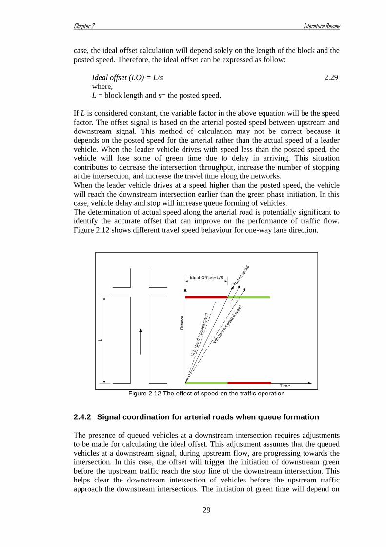
Chapter 2 Literature Review
29
case, the ideal offset calculation will depend solely on the length of the block and the
posted speed. Therefore, the ideal offset can be expressed as follow:
Ideal offset (I.O) = L/s 2.29
where,
L = block length and s= the posted speed.
If L is considered constant, the variable factor in the above equation will be the speed
factor. The offset signal is based on the arterial posted speed between upstream and
downstream signal. This method of calculation may not be correct because it
depends on the posted speed for the arterial rather than the actual speed of a leader
vehicle. When the leader vehicle drives with speed less than the posted speed, the
vehicle will lose some of green time due to delay in arriving. This situation
contributes to decrease the intersection throughput, increase the number of stopping
at the intersection, and increase the travel time along the networks.
When the leader vehicle drives at a speed higher than the posted speed, the vehicle
will reach the downstream intersection earlier than the green phase initiation. In this
case, vehicle delay and stop will increase queue forming of vehicles.
The determination of actual speed along the arterial road is potentially significant to
identify the accurate offset that can improve on the performance of traffic flow.
Figure 2.12 shows different travel speed behaviour for one-way lane direction.
Dist
ance
Time
L
Ideal Offset=L/S
Veh.
spee
d >
post
ed sp
eed
Veh.
spee
d <
post
ed sp
eed
Post
ed sp
eed
Figure 2.12 The effect of speed on the traffic operation
Signal coordination for arterial roads when queue formation 2.4.2
The presence of queued vehicles at a downstream intersection requires adjustments
to be made for calculating the ideal offset. This adjustment assumes that the queued
vehicles at a downstream signal, during upstream flow, are progressing towards the
intersection. In this case, the offset will trigger the initiation of downstream green
before the upstream traffic reach the stop line of the downstream intersection. This
helps clear the downstream intersection of vehicles before the upstream traffic
approach the downstream intersections. The initiation of green time will depend on

Chapter 2 Literature Review
30
how the number of queued vehicles and the service rate at the downstream
intersection. In order to discharge the queued vehicles, the time will be taken from
the green portion devoted for the upstream flow. Figure 2.13 demonstrates the
relationship between the offset estimation and the number of queued vehicles.
Dis
tanc
e
Time
L
Offset=L/s – ( Qh+l)
S=posted speed
Figure 2.13 The effect of queued vehicles on the offset calculation
Figure 2.13 shows that upstream traffic arriving loses green time due to the initiation
of the green signal earlier because of the presence of queued vehicles. This results in
reducing the number of vehicles able to pass through the intersection, increasing the
number of stops and increasing the total stopped delay. A new green time interval
exists due to this operation and can be estimated as follow:
Gn= Go- (Q*h + l) 2.30
where,
Gn = new effective green time,
Go = original effective green time,
Q = number of queued vehicles,
h = discharged headway and
l = start up lost time normally range between (2-4secs).
The capacity of downstream intersection will be impacted negatively as well due to
decreasing green time for upstream flow. Consequently, a reduced capacity can be
calculated as follows:
cd = (Gn / C) * S 2.31
where,
cd = reduced capacity of downstream intersection due to a queue existing,
Gn = new effective green time,

Chapter 2 Literature Review
31
C= cycle length and
S= saturation flow.
Since the capacity of intersection has decreased, the delay and number of stops per
vehicle will increase as well. The capacity and delay at downstream intersection can
be estimated as follows:
New Capacity = Original capacity – Reduced capacity
cn = (Go / C) * S – (Gn / C) / S 2.32
cn = (( Go- Gn) / C) * S 2.33
D = cn * h / 3600 2.34
where,
cn = new capacity due to the queued vehicles,
D = delay in term of number of vehicles, and
h = discharged headway.
The number of queued vehicles at the intersection can identify the performance of
platoon progression and the intersection throughput efficiency. The offset
calculations due to queued vehicles can be determined as follow:
Adjustment offset = Ideal offset - time required to clear the queued vehicles
Offsetadj = L/s – (Qh+l) 2.35
All the symbols in above equation have been defined earlier.
Signal coordination for arterial roads under oversaturated 2.4.3condition
The previous section focussed on the queued vehicles at the downstream intersection
under the condition that the queue doesn’t exceed the block length. When the queue
length propagates back and fills the entire block length of the arterial, in the case of a
short link, the network will block and the coordination of traffic signal loses its
purpose. Figure 2.14 shows that the entire green time at the downstream intersection
has been consumed by the queued vehicles. All new vehicles which approach the
intersection do so during the red phase. The side cross street is also impacted by this
operation because blockage of the intersection area.

Chapter 2 Literature Review
32
Dis
tan
ce
Time
L
Offset=L/s – ( Qh+l)
S=posted speed
Figure 2.14 The operation of traffic flow under using normal offset
Usually signal offsets switch the upstream intersection to green relative to the
downstream intersection. If the length block is filled with vehicles and the upstream
intersection is turned to green, the vehicles would be stacked at the upstream link
and block the network. Because of the upstream blockage, the cross street will also
probably be poorly utilised. In order to avoid this traffic condition, the signal at the
upstream intersection of the main street will turn red instead of green and grant the
cross street a fraction of green time. This type of control is called Equity Offset.
Figure 2.15 shows the traffic light system under those circumstances and the concept
of Equity Offset can be expressed in the following equations.
Dis
tan
ce
Time
L
Sacc =acceleration speed
of congested segment
gC
-L/S
Upstream signal turns red because the spill back (1)
Switch point(1,2)
Cross street turns green (2)
Figure 2.15 Equity offset process

Chapter 2 Literature Review
33
Equity offset (t equity) = g*C – L / sacc 2.36
where,
g = fraction green of main street,
C = upstream cycle length and
sacc= accelerated speed at congested link.
In Figure 2.15, the upstream signal switched red once vehicles at the upstream
intersection start moving. This is intended to flush out all the vehicles
accommodated at the congested section with an accelerated speed to reach about 16
ft/s which tries to ensure that no new vehicles enter the section. At the same time, a
green portion for upstream traffic in the main road is devoted to the cross street in
order to enhance the departure service and to avoid the probability of forming long
queue due to the intersection blockage by clearing the intersection.
VSL and the performance of signalised intersection 2.4.4
VSL has the potential to improve performance by using the speed of the upstream
platoon on the arterial road as a reference to match the initiation of green at the
downstream signal.
Success depends on using the actual variable speed instead of the fixed posted speed.
This procedure requires installation of variable speed signs at each intersection to
guide the drivers to follow a specific speed. The speed sign is linked to upstream
detectors and is synchronised with downstream detectors at each intersection. The
downstream detectors provide traffic information on how many queued vehicles
exist as information to the upstream detectors responsible for computing the desired
speed and subsequent display. Figure 2.16 shows the conceptual operation of VSL.
Figure 2.16 VSL plan
The new technique concentrates on the total time required to clear the downstream
intersection of queued vehicles and the time spent in traversed link. The outcome is
that a new speed will be calculated and displayed to control the upstream flow.
Downstream detectors
Speed signal
Traffic information
Desired speed Upstream detectors

Chapter 2 Literature Review
34
The ratio of length block to the total time spent is used to determine the desired
speed as shown in equation 2.38. The number of queued vehicles represents the main
factor in calculating the desired speed. If the number of queued vehicles is zero the
desired speed will equal the posted speed and the calculation will be as equation
2.29. When vehicles are queued, the speed of upstream traffic can be reduced to
allow clearing the queued vehicle without recalculating the new offset for the
upcoming traffic. The desired speed can be determined through the following
equations:
Total Time Spent = ideal time (ideal offset) + time needed to clear the queued
vehicles
TTS= (L/s) + (Q*h+l) 2.37
Desired Speed (DS) = L / TT 2.38
VSL use when the queued vehicles consume the entire green 2.4.5interval
Customarily, the spilt cycle for a long length block would be less than the spilt cycle
for short consecutive links. This procedure raises the efficiency of flow at short
lengths and reduces the effect of queue spill back towards the upstream intersection.
VSL focusses on keeping the offset calculation constant and controlling the speed of
vehicle through the arterial road. Figure 2.17 shows vehicles queued at the stop line
waiting the green signal which resulted in consuming the full green interval.
L
Ideal offset
S=posted speed
Delay
Delay
Queued vehicle occupy the full green portion
Downstream intersection
Upstream intersection
Figure 2.17 Offset operation pre-speed limit initiation
In this case, the arrival traffic will not able to pass the downstream intersection
during the cycle and vehicles will be forced to stop at the back of the queue or at the
start of the red signal. This traffic pattern can negatively influence the performance
of arterial roads by increasing the number of stops that then reduce the safety and
increase the queue length that may lead to breakdown the traffic flow.
In order to overcome such traffic situations, the speed of arrival traffic is managed
by the application of a speed less than the posted speed.
Figure 2.18 shows the trajectory of arrival flow towards the downstream intersection
under pre and post speed control.

Chapter 2 Literature Review
35
L
Ideal offset
S
Delay
Delay Downstream intersection
Upstream intersection
Scontrol
Arrival flow post- control
Arr
ival
flow
pre-
con
trol
Queued veh.
Figure 2.18 Arrival flow under post- speed limit control
The speed of arriving vehicles can be determined by the following equations:
tideal= L/s 2.39
tqueued veh= Qh+l 2.40
Scontrol = L/ (tideal + tqueued veh+ r) 2.41
where,
Scontrol = controlled speed that needed to manage the arrival flow,
r = fraction of upstream red signal and
L= length block.
Applying VSL under spill back conditions 2.4.6
The function of equity offset was discussed earlier, proposing a red signal for the
upstream flow and granting the green time for the side street when the spillback
spread towards the upstream intersection. This maintains arterial functionality when
the spillback occurs from the main street or cross street.
VSL can be used to achieve similar functionality but differs in the operation and
outcomes. The new concept proposes that vehicles within the through lanes at the
upstream intersection progressing towards the congested intersection should be
restricted using speed signal signs while the left and right turn lanes continue
working. The method may assist to ensure good traffic flow for both the main street
and side cross street. It should also, reduce or mitigate the effect of spillback on the
downstream intersection by controlling the upstream traffic.
This method may not affect the flow of side cross street and may eliminate the
likelihood of a queue propagating due to the main street backup. Figure 2.19
illustrates the mechanism of employing speed signal sign at upstream intersection.

Chapter 2 Literature Review
36
L
S=o
S=o
Mai
n s
tre
et
Cross street
L/Sacc
gC rC
S acc=
acc
eler
ated
spe
ed
on c
onge
sted
link
S
Upstream intersection
Downstream intersection
Posted speed
Figure 2.19 Schematic of using new spill back management
The following points can be taken from the figure above:
1. The offset at downstream intersection will not switch the green light at upstream
intersection to red signal as in normal offset (i.e. equity-offset function). The green
interval will retain a switch-on under condition of limit the speeds of through
movement towards the upstream traffic. The value of the speed limit will be based
on the length of queue at downstream intersection. In some traffic conditions, the
speed limit is set out to zero in order to prevent only the through movement and
allow the left turn movement.
2. The application of this method will retain the signal timing of cross street constant
and prevent right turn vehicles from the cross street entering the main road at this
congested period. Unlike the normal management that gives opportunity to the
cross street vehicles to turn into empty spaces for main road during the spillback
period.
The offset calculation for upstream intersection under spill back condition can be
determined as follow:
tequity = g*C – L / Sacc 2.42
tspeed technique = L / S + (r * C - (g * C – L / Sacc) 2.43
tspeed technique = L / S + r * C - tequity 2.44
where,
L= length block,
S= posted speed,
r = red portion of upstream intersection,
C = cycle length of upstream intersection and
Sacc= accelerated speed on the congested link.

Chapter 2 Literature Review
37
Using VSLs in urban areas 2.4.7
To understand the benefit of using the new approach, the congestions in
conventional traffic moving toward the urban area is briefly explained. Figure 2.20
represents a schematic drawing for a roadway operation-containing bottleneck
towards urban areas. The bottleneck is located where the flow capacity upstream
( )is higher than the flow capacity downstream (
) of the bottleneck
location. It can be seen from the figure that is the maximum flow that could
be maintained at the bottleneck situation if the arrival flow ( ) equal or less than
the . On the other hand, traffic congestion is formed when the arrival flow
( ) is higher than the . Thus, the congestion head is located at the bottleneck,
whereas the tail of the congestion is moving towards traffic upstream causing a net
gridlock. This traffic flow phenomena appears clearly during the peak periods, that is
when the traffic volume on the road is high.
Figure 2.20 Bottleneck activation view of roadway without using VSLs
Basically, the new approach is based on controlling the arrival traffic (qin) of
bottleneck using variable speed limits technique in order to form an optimal traffic
flow performance for travel demand. A local aspect for this approach is illustrated in
Figure 2.21.
Figure 2.21 Schematic view of roadway traffic flow control using VSLs
The bottleneck indicated in Figure 2.21 does not cause up stream congestion (and no
control strategy is needed) as long as ≤ . Once grows larger than the
bottleneck capacity , the bottleneck will be activated without any control
strategy as seen previously in Figure 2.20. The primary aim of the new approach is
to control the flow to be equalized to the bottleneck capacity. This can be
achieved by implementing the variable speed limits (VSLs) to control the amount of
trips on the main roads, i.e. decreasing the traffic volume by reducing vehicles’
𝐪𝐜𝐚𝐩𝐮𝐩𝐬𝐭𝐫𝐞𝐚𝐦
Active Bottleneck
qout≤qcap.down Congestion qin
Controlled Congestion
𝒒𝒄𝒂𝒑𝒅𝒐𝒘𝒏 𝒒𝒄𝒂𝒑
𝒖𝒑𝒔𝒕𝒓𝒆𝒂𝒎
Bottleneck
Flow control
qout
qc

Chapter 2 Literature Review
38
speed. A roadway congestion will be formed upstream of the roadway traffic flow
control location where vehicles approaching this area with relatively low speed
related to controlled upstream traffic . Traffic flow can be enhanced in the urban
areas by VSL and the reduction in the speed might result in decreasing the total
delay of the traffic. In other words, there will be an increase in the performance of
the traffic. Hegyi et al. (2005) found that the congestion after a breakdown has a
reduction in the outflow by about 5-10%. Consequently, any control strategy
improving the breakdown may attain 5-10% improvements in the outflow rate.
Mathematical approach of VSLs in urban areas 2.4.8
The macroscopic description of traffic flow implies the definition of adequate
variable expression the aggregate behaviour of traffic at certain times and locations.
The discrete time step is denoted by T in second where m is divided into
segments of equal length in meter as indicted in Figure 2.22. The traffic in each
segment of link m at discrete time is macroscopically
characterized via the following variables:
1. Traffic density ( ) (veh/km/lane), is the number of vehicles in segment of link m at time divided by and by the number of lanes,
2. Mean speed ( ) (km/h), is the mean speed of the vehicles included in
segment of link m at time , and
3. Traffic volume or flow ( ) (veh/h) is the number of vehicles leaving
segment of link m during the time period [ ( ) ] divided by T.
Figure 2.22 Schematic view of traffic flow details
Basically, the new model is based on the evaluation of total delay during any critical
periods with reference to the utilization VSLs. The simulation of this concept can be
conducted using VISSIM software. Usually, when the travel demand ( ) becomes
higher than the in the main roads, VSL can be applied to avoid forming the
bottleneck by forcing lower speeds (critical speed, ) in the critical section. The
critical speed value acts as a benchmark to organize the entire preceding traffic
towards the critical area via sending a variable signal message (VSM) at each
intersection. Generally, the speed will be decreased gradually over the whole road
until the critical speed that caused the bottleneck is reached. Therefore, the entire
delay created by this strategy which includes three stages, will be adopted to
compute the total delay of vehicles utilizing the roadway as below:
1. Compute the critical speed that leads to the formation of a bottleneck in a
segment i (critical segment).
Link m
i-1 in i
n-1
𝑞𝑚 𝑖

Chapter 2 Literature Review
39
2.45
where,
= critical speed that causes bottleneck at segment , = discharge rate for segment ,
= traffic demand for segment and
, = traffic density for out and in respectively, for segment
2. After determining the critical speed that causes bottleneck for segment , this
speed will be used to organize the inbound traffic on each of the other segments
preceding the segment i.
[ ] 2.46
[ ] 2.47
where,
controlled speed at segment i-1that close to critical segment,
= controlled speed at final segment on link m, and
= free flow speed for segment
3. After computing a new controlled speed value for each segment of link m,
delay can be estimated in three stages, as described below:
Stage1: Delays caused by reducing speed limit for links approaching critical
segment.
∑ (
-
) 2.48
where,
= entire approached delay due to reducing speed in each segments in sec, and
= length of each segment in meter.
Stage2: Delays due to acceleration of vehicles after the critical segment.
=( )
2.49
Where,
= delay from acceleration after passing critical segment,
= vehicle acceleration value (constant value),
= critical sped that causes bottleneck.
Stage3: Delays caused by stochastic queuing (delays due to waiting time in queue).
( ) 2.50
where,
= stochastic delay (hr).
Eventually, the total travel time estimation using VSL application includes three
components, delay from reducing speed limits in segments approaching the critical
segment ( ), delay from acceleration of vehicles after passing the critical
segment ( ) , and delay yielded from stochastic queuing ( ). This result
assumes that delay presented from traffic lights is constant, in order to facilitate
understanding the VSL module. This value will be compared with the base value of
delay without any control measures to reveal the improvement of using VSL on

Chapter 2 Literature Review
40
decreasing the delay during the peak period. Figure 2.23 shows a flow chart for the
VSL process.
Figure 2.23 VSLs control algorithm
Summary 2.5
From the extensive review of the literature, it has been concluded that the issue of
traffic congestion in urban areas remains a continuing problem and that much
research is ongoing. Previous studies of congestion in urban areas have involved
pricing, and transfer of congestion. Research has aimed of reducing the inlet traffic
towards the congested links during the peak period that result in maximising traffic
throughput, minimising delay and enhancing traffic safety. The available research on
Variable Speed Limit controls has shown their potential for reducing congestion on
motorways. However, VSLs has not been used on urban arterial road networks to
alleviate congestion, as an urban road network is a more complex control challenge
than a motorway. This research helps address that challenge.
Sensor
No
Yes, T=0, k=1
Displayer
Collect traffic data for upstream & downstream
Flow rate, density, speed
Compression between upstream & downstream
If in >
Compute initial controlled speed v r that causes
bottleneck
Compute optimal controlled speed for each
segment
Display controlled speeds at entrance of each
segment
K=2
Repeat steps for other
intervals

Chapter 3 Survey & Data Collection
41
3 CHAPTER THREE
Survey & Data Collection
Introduction 3.1
This chapter provides the rationale for selecting the Griffith Arterial Road (GAR) in
Brisbane as a case study area for the present research. It also explains in detail the
methods used to collect the relative traffic data.
Three sources of data were integrated to evaluate the traffic performance of the
selected area. First, Synergised Transport Resources Ensuring an Advance
Management System (STREAMS) data was obtained from the Queensland
Department of Transport and Main Roads (QDTMR). STREAMS is based on a
database of loop detector records. Second, field observations were conducted using
video cameras and manual counting to determine vehicle types (truck, bus, and car),
existing traffic volumes, traffic lane configuration and average headway at the
signalised intersections on the GAR. Virtual Dub Software (VDS) was used to
facilitate counting traffic volume and to precisely identify the traffic flow
configuration. Third, a floating car survey (FCS) along the study area was
implemented to estimate travel times on the arterial road. Based on estimated travel
time data and VISSIM (Verkehr in Städten-Simulations) software features, optimum
offsets between the signalised intersections were identified. Figure 3.1 illustrates the
design of the survey that was conducted in the study area. A full description of the
data collection, methods and traffic survey procedures are discussed in the following
sections.

Chapter 3 Survey & Data Collection
42
Figure 3.1 Survey design
Selection of study area 3.2
Griffith Arterial Road U20 is part of the Brisbane Urban Corridor (BUC), and is
approximately 11.5 km long and lies between the Gateway Motorway and the
Ipswich Motorway. It is part of the Australian National Land Transport Network.
The arterial road is under the jurisdiction of the Queensland Department of Transport
and Main Roads (QDTMR). The corridor consists of three main sections Granard
Rd, Riawena Rd, and Kessels Rd and involves several signalised intersections. These
are the intersections of Granard Rd - Beatty Rd, Granard Rd - Beaudesert Rd -
Riawena Rd, Riawena Rd - Perrin Place, Riawena Rd - Orange Grove Rd, Kessels
Rd - Troughton Rd, and Kessels Rd - Mains Rd. Figure 3.2 (a),(b) show the location
of U20 captured from Google earth website. Figure 3.3 shows the layout of the study
area and Table 3.1 provides the names of intersections along Griffith Arterial Road
U20. Table 3.2 shows the number of lanes at each approach of the intersection.
Study area selection
Pilot investigation
Data collection
STREAM database Field observation Floating car survey
Video cameras &
Manual counting Loop detectors Floating car test
Traffic data
Geometric data
Google earth &
Field measurements
Travel time Existing traffic volume
Traffic configuration
Vehicle class
Signal phases
Traffic volume for
main road only
Speed distribution

Chapter 3 Survey & Data Collection
43
(a)
(b)
Figure 3.2 U20 Griffith Arterial Road, Brisbane, Queensland (QLD), Australia
According to the field observations and QDTMR data, the eastbound (EB) and
westbound (WB) directions of this corridor experience heavy congestion during the
morning and evening peak traffic periods especially at the intersection of Granard Rd
- Beaudesert Rd - Riawena Rd and Kessels Rd - Mains Rd.
The average daily traffic volume count (ADT) for this corridor is approximately
18,000-24,000 vehicles. The distances between intersections varies and ranges from
0.4 km to 1.5 km. The two ends of the corridor have closely spaced signalised
intersection approximately 400m apart whereas in the middle section of the corridor
the intersections are approximately 1 km to 1.5 km apart. The speed limit varies
along the length of the road. The shorter links have speed limits of 60 km/hr and the
longer links have speed limits of 70-80 km/hr.
The number of lanes at approaches to the signalised intersections varies from 1 to 4.
In addition, the arterial links between the intersections have from 1 to 3 lanes in each
direction. Multiphase traffic signals control all intersections along U20, with a cycle
length 120-160 seconds during the daytime. The study area had high volumes of
heavy trucks (3% to 18%) during the survey period especially on the EB and WB
N
N
Brisbane

Chapter 3 Survey & Data Collection
44
lanes. This may be due to the adjoining land uses. The area is characterised by
multiple land uses including residential, heavy and light industry, retail and
commercial activities, and freight companies.
Figure 3.3 Study area layout
Table 3.1 Intersection names
Intersection
Number Intersecting Roads
Distance to next
intersection (m)
1 Granard Rd- Beatty Rd 400
2 Granard Rd - Beaudesert Rd - Riawena Rd 1015
3 Riawena Rd - Perrin Place 978
4 Riawena Rd - Orange Grove Rd 1062
5 Kessels Rd - Troughton Rd 1541
6 Kessels Rd - Mains Rd 639
Table 3.2 Number of lanes
Intersection
Number
Number of lanes at each approach
NB SB EB WB
TH RT TH RT TH RT TH RT
1 1*
1 1 1 3 1 2
1
2 3 1 3 1 2 2 3 1
3 0 2 0 0 2 1 2 0
4 2 0 2 1 3 1 3 0
5 1*
1 1 1*
3 1 3 1
6 3*
1 3*
1 3 1 3 1 * Refers to a shared TH/RT lane
Key characteristics that lead to the selection of Griffith Arterial Road U20 as a case
study are:
1. The availability of traffic data, provided from QDTMR assisted in understanding
the traffic situation along the road.
2. The strong support received from QDTMR to carry out the field traffic survey.
3. It is a major urban arterial road with periods of high congestion.
4. It has high daily traffic volumes.
5. The diversity of adjoining land use activities may have a negative effect on the
performance of proposed traffic scenarios for the road. This provides an
opportunity to examine the efficiency of any proposed traffic management
actions.
6. Short links with recurrent congestion (morning/evening peak) and long links with
high speeds occurring at the same times satisfied the traffic pattern requirements
for testing the proposed management plan.
6
5 4 3 2 1

Chapter 3 Survey & Data Collection
45
7. Traffic management strategies were already implemented at the site such as
adaptive traffic control and coordinated traffic systems however, some places still
experienced traffic degradation due to high traffic demand. New traffic
management strategies had the potential to alleviate the risk of traffic degradation.
Data Collection 3.3
Traffic data was collected from the study area on Wednesday, July 11, 2012 for the
peak period between 3:30 pm and 5:30 pm with the cooperation of QDTMR. Traffic
flow, traffic distribution, vehicle type and traffic headway were collected by using
high-resolution video cameras at each intersection. Public holidays and school
holiday were avoided. Data were collected from three sources as explained in the
following sections.
QDTMR database 3.3.1
Initially traffic data regarding the study area was collected from the Queensland
Department of Transport and Main Roads (QDTMR) database. QDTMR uses an
adaptive traffic control (ATC) system STREAMS, which is based on detector
records. For the GAR these detectors were placed on the main eastbound (EB) and
westbound (WB) traffic streams at a distance of 35-40 meters from the intersection
stop line. STREAMS data were collected for five days (Tue 7, Wed 8, Thu 9, Tue 14
& Wed 15 Sep 2010) from 07/09/2010, 12:00:00 am to 15/09/2010, 12:00:00 am.
Data was collected every 2 seconds and included traffic volume, expected cycle
length, posted speed, expected travel time and occupancy.
This data was used to select the appropriate day for the survey, identify the heaviest
peak traffic periods for morning and evening intervals and determine the speed
distribution along the road. These issues are discussed briefly in the following
sections.
3.3.1.1 Selection of survey day
In order to identify which day had the highest traffic volume, STREAMS data was
analysed to find the highest daily traffic over two weeks of data. This step is
important because the application of VSLs is recommended for use during
congestion periods and when the volume to capacity ratio (v/c) approaches 1,
otherwise the application will not be effective.
Table 3.3 shows the distribution of average daily traffic (ADT) along the EB arterial
road during five normal workdays. The EB direction includes five arterial links
(Beatty-Beaudesert link, Beaudesert-Perrin link, Perrin-Orange link, Orange-
Troughton link and Troughton-Mains link). In this table, Thursday and Wednesday
have the highest traffic counts followed by Tuesday. Thursday has one period of
high traffic volume while Wednesday has two periods of high traffic volume. Since
Wednesday has two high traffic volume periods and is close to Thursday traffic
volume it was selected as the traffic survey day.
Figure 3.4 shows the average daily traffic for five days. The link experienced only a
small variation in ADT over the five days indicating that it was operating with nearly
constant traffic demand during the survey period. Thursday’s data had the highest
ADT for all links followed by Wednesday and lastly Tuesday. Thursday and
Wednesday were chosen as the days on which to collect data.

Chapter 3 Survey & Data Collection
46
Table 3.3 ADT for two weeks survey
Link EB Direction
STREAMS data surveying
1 2 3 4 5
Tuesday
7th
Sep
2010
Wednesday
8th
Sep
2010
Thursday
9th
Sep
2010
Tuesday
14th
Sep
2010
Wednesday
15th
Sep
2010
1 Beatty-Beaudesert 9927 11174 11807 10553 11600
2 Beaudesert-Perrin 16727 17453 18146 17146 17757
3 Perrin-Orange 13255 14035 14429 13236 14461
4 Orange-Troughton 17305 17791 17920 16685 17677
5 Troughton-Mains 15061 16375 16846 15653 16580
ADT 14455 15366 15830 14655 15615
Figure 3.4 ADT for EB arterial links
3.3.1.2 Determination of peak periods
Because VSL was planned to be used to optimise traffic performance, it was
important to select the peak periods of traffic flow. In order to capture accurate
variations in traffic flow, count intervals of 15 minutes were used. This interval is
recognised as being the shortest interval for which a stable flow exists.
The data collected from the STREAMS database, calculated for each 2 seconds
interval, was aggregated for each 15-minute period. Normally two peak periods are
considered during the day, morning and evening. Figure 3.5 and Figure 3.6 show
hourly traffic volumes for the EB morning period (MP) and WB evening period (EP)
respectively. The EB traffic was investigated from 6:00 am to 12:00 pm and the WB
traffic was investigated from 12:00 pm to 7:00 pm.
Figure 3.5 shows that the morning peak starts at 7:30 am and continues to about
10:15 am. It is dominated by a large number of commuters going to work during this
period. In addition, the trend of volume variation is quite noticeable for the EB
morning period and the WB evening period. The links that contribute a high volume
to the EB direction showed less contribution to WB direction and vice versa. One of
the characteristics of the U20 route is that it is more of a circumferential route, rather
than a radial route. Therefore, peak hour traffic is not dominant in any one direction.
Figure 3.6 shows no clear WB evening peak. This occurs because the variation in
traffic volume is small for long periods. This may cause small variations in hourly
volume and less shift in travel behaviour where drivers try to travel during the off
peak period to avoid encountering the peak period. However, the evening peak
0
2000
4000
6000
8000
10000
12000
14000
16000
18000
20000
7TU 8WE 9THU 14TU 15WE
AD
T
Weekdays
Troughton To Mains Orange to Troughton
Perrin to Orange Beaudesrt to Perrin

Chapter 3 Survey & Data Collection
47
period is more concentrated and this concentration is mostly from 3:30 pm to 5:30
pm. It is dominated by commuters returning to their residences after their day’s
work. For study purposes, the evening period was selected as the primary data
collection and modelling period.
Figure 3.5 Variation in traffic volumes at the EB direction
Figure 3.6 Variation in traffic volumes at the WB direction
3.3.1.3 Performance indicators in STREAMS system
In this section, some of the performance indicators for the road network operations
are investigated. Usually, traffic performance data are collected a few times a year
using the same methods for data collection and analysis. In recent years researchers
have concluded that the limited amounts of survey data available are inadequate to
present a true picture of prevailing traffic situations especially for mega cities with
long peak traffic periods. Some jurisdictions have attempted measuring live traffic
flow characteristics for freeways and arterials. Such measurements are based on
using vehicle detectors in freeway management systems (FMS) and signal area
traffic control (ATC) systems to identify traffic performance. Five indicators have
been proposed to evaluate the performance of traffic conditions for both freeway and
arterial control systems. These indicators are however considered controversial by
0
50
100
150
200
6:0
0
6:1
5
6:3
0
6:4
5
7:0
0
7:1
5
7:3
0
7:4
5
8:0
0
8:1
5
8:3
0
8:4
5
9:0
0
9:1
5
9:3
0
9:4
5
10:0
0
10:1
5
10:3
0
10:4
5
11:0
0
11:1
5
11:3
0
11:4
5
12:0
0
Vo
lum
e (v
eh/h
r)
Time (AM)
Beatty-Beaudesert link MP(EB) Beaudesert-Perrin link MP(EB)Perrin-Orange link MP(EB) Orange-Troughton link MP(EB)Troughton-Mains link MP(EB)
0
50
100
150
200
250
12:1
5:0
0
12:4
5:0
0
1:1
5:0
0
1:4
5:0
0
2:1
5:0
0
2:4
5:0
0
3:1
5:0
0
3:4
5:0
0
4:1
5:0
0
4:4
5:0
0
5:1
5:0
0
5:4
5:0
0
6:1
5:0
0
6:4
5:0
0
Vo
lum
e (v
eh/h
r)
Time (PM)
Beaudesert-Beatty link EP(WB) Perrin-Beaudesert link EP(WB)
Orange-Perrin link EP(WB) Troughton-Orange link EP(WB)
Mains-Troughton link EP(WB)

Chapter 3 Survey & Data Collection
48
Troutbeck et al. (2007). A brief description and example calculations of these
indicators is provided in the following sections:
1. Traveller Efficiency (Travel Speed): This parameter indicates the traffic
congestion in terms of speed. On a freeway, spot speed of vehicles can be
determined using sensors such as loop or microwave detectors. On arterial roads, it
can be calculated using two methods, sensors and traffic signal systems. The spot
speed information provided from sensors does not indicate the actual speed along the
arterial road. This is because speeds vary along the arterial link and are significantly
affected by the signal timing and the quality of platoon progression.
Normally speed calculations will be determined from signal area traffic control
(ATC) by counting the inverse of travel time for vehicles that traverse the link.
Estimation of travel times from signal setting or ATC requires converting the travel
time to spatial speed in order to estimate the effect of signal settings on speeds. The
calculation of travel speed can be explained as follow, (Troutbeck et al, 2007):
, ,
, ,
( , , )i t d
i t d
LTS i t d
ATT
3.1
where,
TS(i,t,d) is travel speed on link i at time t and survey day d,
L is the length of link i and ATTi,t,d is the average travel time on link i at time t and day d.
In order to calculate the effect of flow on the speed of vehicles during the survey
period, the flow for each link along the network was considered in estimating the
average travel speed.
The average travel speed (ATS) for a network can be calculated as:
, ,
, ,
, , , ,
, ,
( )
( / ( , , ))
i i t d
i t d
i t d i t d
i t d
LV
ATSL V TS i t d
3.2
where, Vi,t,d is the flow on link i monitored in time t and day d.
2. Traveller Efficiency (variation from posted speeds): This parameter calculates
the deviation from the posted speed limits for the road network. The deviation in
travel speed can be computed as :
(%) ( )*100 /SpeedVariation PostedSpeed AverageSpeed PostedSpeed 3.3
The average speed can be determined from on the spot speeds on the freeway or as
the inverse of travel time obtained from the ACT on arterial roads.
3. Reliability (travel speed): This indicator measures the variation in speeds based
on the coefficient of variation (the standard deviation over the mean). It can be
displayed as the proportions of the road network experiencing different levels of
variability per unit time. Customarily, the travel times for arterial roads can be

Chapter 3 Survey & Data Collection
49
obtained from the signal settings of the ATC system and their reciprocals are utilised
to estimate the speed reliability. The traffic flow has various route destinations, so
the route variability can be determined as follow:
Route variability 1.44 / 100k k kRV SD T 3.4
Where Tk is the mean travel time on route k measured in units of min/km and the SDk
is the standard deviation of travel times on route k in (min/km).
1
N
n
nk
t
TN
3.5
2
1
( )
1
N
n k
nk
t T
SDN
3.6
where,
N= is the total number of travel time samples tn on route k.
1.44 = represents the calculation factor for 85% confidence interval.
The sample size for the calculation is usually 15 min for all surveys.
4. Traffic productivity: This indicator represents the product of speed and flow.
High traffic productivity can be achieved when the speed indicates free flow speed
and the flow reaches the traffic capacity. Low productivity occurs due to low traffic
flow and/or low speed. In addition, low productivity can be attributed to low traffic
demand and does not necessarily reflect poor performance for the road network. It is
shown as the proportion of a network at various levels of productivity over time. The
productivity can be illustrated as:
**100
*nom nom
speed flowproductivity
speed flow
100
if speed < speednom
if speed ≥ speednom
3.7
3.8
Where, speednom and flownom represent the normalisation speed and flow for the road
network before the productivity starts to decrease (traffic congestion).
Table 3.4 indicates the recommended normalisation values to identify optimal
conditions. The productivity of speed-flow equal to or greater than 100 indicates that
the network is operating at good level of service during the specified period.
Table 3.4 Speed and flow normalisation values
Parameters Arterial road Freeway
Normalisation speed 35 km/h 80 km/h
Normalisation flow 900 veh/h/lane 2000 veh/h/lane
Source: (Troutbeck et al. 2007)
To sum up, STREAMS data can be extracted from data detectors and is useful to
identify peak time-periods and the appropriate days for conducting field surveys of

Chapter 3 Survey & Data Collection
50
selected area. The present study used VISSIM software to analyse and investigate
the effectiveness of VSL application. This software requires a lot of traffic
information about the road network to execute the simulations correctly.
Data collected from detectors does not provide all the traffic data needed to test the
proposed traffic scenarios. Field data collection is necessary because:
1- STREAMS data were collected for only the EB and WB directions and no
data was collected for the intersecting SB and NB roads.
2- The traffic volumes counted by detectors represent the total volume travelling
in that link. There is no count of the number of vehicles turning at each
intersection.
3- Vehicle type (truck, car, bus) is not recorded within the detector database
and vehicle composition needs to be known to determine the percentage of
heavy vehicles (% HV).
4- The loop detectors database had some unrealistic traffic volumes which
suggested the readings were unreliable for traffic analysis.
For these reasons, additional field data were collected to overcome the unreliable
counter data and to complete the missing parts of the collected data.
The following sections discuss in details how the field data survey was conducted.
Field data 3.3.2
In order to gain accurate data about the traffic flow in the selected study area, manual
counting and video counting were used to supplement STREAMS data. The
procedures for collecting field data were as follows.
3.3.2.1 Pilot survey
Before undertaken the detailed survey in depth, a pilot survey of the selected study
area was performed to identify the best locations, the number of video cameras
needed and the number of observers required doing the manual counting. This step is
crucial to minimise errors that could be made during the production survey, and to
increase survey accuracy. The preliminary survey was conducted to determine:
1- The number of video cameras needed to conduct the survey and the number
of video cameras required to be available as standby in case of malfunction in
one of the cameras.
2- The time needed to install the video equipment on the site. A check was also
made on the battery capacity of cameras, to ensure the video recording could
be performed with no stoppages.
3- The number of persons needed to manage and control both the video
monitoring and perform the manual counting at each intersection.
4- Safe locations for positioning each video camera.
5- The appropriate safe working requirements needed to minimise the risk to the
survey staff.
3.3.2.2 Video cameras set up and manual counting distribution
Despite the recent advances in technology regarding traffic data collection, some
traffic data still needs to be collected manually. Situations requiring manual surveys
include short duration surveys or surveys focused on specific locations such as
signalised intersections. The data collection for this study required two types of

Chapter 3 Survey & Data Collection
51
surveying: manual counting conducted by hand counters, and video recording using
High Definition Cameras (HDC).
Six video cameras were deployed along Griffith Arterial Road (GAR) U20. One
camera was allocated for each intersection at a position which enabled coverage of
all the traffic movements at the intersection. Some of the intersections are very wide
and one camera was not capable of capturing all traffic movements at the
intersection. The data missing in the video recording were always found to be the
turning of vehicles. Therefore, manual counting during the video recording was
implemented for some left turning movements. Both methods of data survey were
used at intersections 2 and 5. Table 3.5 and Figure 3.7 outline the deployment of
video cameras and manual counting for the study area.
A group of 18 people conducted simultaneous counts along the route. The large
group were divided into two smaller groups: group number 1 was responsible for the
video processing where two persons were allocated to each camera; and group
number 2 was responsible for manually counting the missing left turn vehicles. Two
people were allocated to record each turning location.
Figure 3.7 Video camera locations
Table 3.5 Video camera locations and manual traffic recording
In order to ensure accurate data collection, instructions were given to each survey
group to start counting and videoing exactly at 3.30 pm and terminate processing at
5.30 pm. Video cameras and observers were positioned on site half an hour before
the survey period to ensure good data collection.
All camera types used in the area were Sony models with high definition (1980×
1080 pixels) and high capacity capable of sustaining videoing for more than two
hours. Each camera was mounted on a tripod at a height of 1.5 metres from the
Intersection
No. Intersection Name Video Camera No. Manual Counting
1 Granard Rd- Beatty Rd 1 None
2 Granard Rd - Beaudesert Rd -
Riawena Rd 2
Left turn for EB
and NB
direction
3 Riawena Rd - Perrin Place 3 None
4 Riawena Rd - Orange Grove Rd 4 None
5 Kessels Rd - Troughton Rd 5 Left turn for EB
6 Kessels Rd - Mains Rd 6 None
6
5 4
3
2
1
Ca1
Ca2 Ca3 Ca4 Ca5
Ca6

Chapter 3 Survey & Data Collection
52
ground. The video tapes of these intersections were used to get accurate volume
counts and vehicle classification along the road network.
Tally sheets were used to record the left turning movements for intersections 2 and 5
at 15 min intervals. Since two observers were available to do this task, each recorder
was responsible for counting either small vehicles or heavy vehicles. This process
reduced the counters’ errors by allowing them to concentrate on one vehicle type
instead of two. The road geometry for these turning movements comprised only one
travel lane. This made the situation for counting easy for the counters. Figure 3.8
shows a photo taken from the video recording for intersection 1. Video counts are
considered more accurate than manual or loop detector counts because:
1- Manual counts may become inaccurate due to human errors associated with
the counting process. Human counters may find it difficult to track more than
one vehicle at a time when several different vehicle movements are involved.
Also, some observers may not be able to count the movement of left on red
because the counters were focused on counting vehicles turning movements
for other directions.
2- Loop detectors are not necessarily accurate for counting high traffic volumes
under congested conditions. Loop detectors are governed by a threshold
value that establishes the presence of vehicles. Therefore, the accuracy of
counting traffic volume will be affected by this threshold.
3- The ability to replay the videotape (more than once) provides the opportunity
for increased accuracy from video counts because the human counter can
focus on a single movement and once finished can replay the video and count
other movements.
Figure 3.8 Snapshot photo for intersection 1
Field data processing 3.3.3
After videoing the traffic conditions along the study area, data processing is needed
to determine the traffic volumes, vehicle types, traffic distribution and discharge
headways at each individual intersection. The data processing was performed by
using video software as outlined in the following sections.

Chapter 3 Survey & Data Collection
53
3.3.3.1 Virtual dub video software
It is difficult to extract the traffic information precisely and directly from videotapes
because the speed of display is relatively high, making traffic counting
unmanageable. Therefore, Virtual Dub Version 1.6.15.0 was used to facilitate the
data processing (Brust et al., 2009). Virtual Dub software (VDS) is a video capture
and processing utility developed by Microsoft written in C++ language and
compatible with 32-bit and 64-bit Windows systems. It is designed to deal with
formats such as MP4, MOV, AVI, WMV, BMP and MPEG but not with Advanced
Video Codec High Definition (AVCHD) format. Cameras with high resolution store
the video file in AVCHD format therefore the video files obtained in this study
needed to be converted to a format to match with the VDS. The benefit of using
Virtual Dub is that it provides much more information than can be collected by
pneumatic road tube detectors as up to 50 frames per second can be taken. It also
provides more flexibility in processing data because the videotape can be stopped,
rewound and replayed if some details are missed. The drawback in using this
software is the large amount of time required and tediousness of the job. However,
the results are of greater accuracy. Figure 3.9 shows an image for intersection 2
captured by Virtual Dub software.
Figure 3.9 Virtual Dub snapshot for intersection 2
3.3.3.2 Field traffic volumes analysing
Traffic volumes were counted for 15-minute intervals for all the travel movements in
the selected study area of U20. Data was aggregated to vehicles per hour for the two-
hour survey. Vehicle class (Truck or car) were also recorded in order to determine
the percentage of heavy vehicles (HV) in the network. The percentage of heavy
vehicles fluctuated from link to link and from one intersection to another. This
variation is due to the demography of the network. The demography of the study
area is distinguished by commercial and industrial services. The percentage of heavy
vehicles varied from 3% to 18%. The highest level of HV was in the NB direction
for intersection 3 due to the large number of freight companies in the area around
this intersection.
Figure 3.10 shows the traffic volume distribution for the two-hour survey during the
evening peak for intersection 1. This volume was collected from the video record of

Chapter 3 Survey & Data Collection
54
camera 1. No manual counting was conducted at this site. The figure shows the EB
and WB directions have the highest volume during the evening period whereas the
NB and the SB directions have the lowest volume. This highlights that the EB and
the WB directions are the main roads while the others directions are considered
minor roads. The variation in traffic volume between EB and WB can be noticed
during the first hour of the survey and this variation disappeared during the second
hour when the two directions reached the same level of traffic volume. The variation
in volume from one interval to another is between 5% and 10% during the evening
peak. This shows that the intersection carries reasonable constant vehicular traffic
during this time. The signals at the intersection are set to operate on a pre-timed
setting during this period.
Figure 3.10 Traffic distribution at intersection 1
The traffic composition on the approaches to this intersection varied from approach
to approach and over time. Figure 3.11 indicates the variation of traffic composition
during the survey period for intersection 1. The rate of HV traffic changes from 4%
to 12% over the four approaches. The high percentages are for the WB and EB
directions during the first hour of survey (3.30-4.30 pm). During this period, HV
traffic had more affect on the performance of traffic flow than during the second
hour of the survey. The percentages of HV were 10% for the EB direction and 12%
for the WB direction during 3.30-4.30 pm and 6% for both directions during 4:30-
5:30 pm.
0
100
200
300
400
500
600
Vo
lum
e (v
eh/h
r)
PM Peak (min)
Intersection 1 EB WB SB NB

Chapter 3 Survey & Data Collection
55
Figure 3.11 Variation of HV for intersection 1
Figure 3.12 illustrates the variation in traffic volume at intersection 2. The traffic
flow for the EB and WB directions followed the same trend over the afternoon
period. This means the traffic volume was equal along these approaches during this
period. The EB and WB directions carried the highest volume in contrast to the SB
and NB directions at intersection 2. The NB and SB directions also carry a heavy
traffic volume during the time of the survey. The volume fluctuated between 300 and
500 vehicles per each 15 minutes. Traffic volumes for intersection 2 were more than
for intersection 1 in all four directions. This confirmed the classification of
intersection 2 as a major intersection by QDTMR.
Figure 3.12 Traffic variations at intersection 2
Figure 3.13 illustrates the distribution of HV at intersection 2. The profile of HV for
intersection 2 is similar to the profile for intersection 1 where the EB and WB lanes
have the highest level of HV traffic. The rate of HV traffic for 3.30-4.30 pm ranges
from 6% to 9% while the second hour experienced a decrease in the percentage of
HV for all the lanes from 4% to 7%.
0
2
4
6
8
10
12
14
EB WB NB SB
% H
V
Intersection approaches
% HV 3:30-4:30
% HV 4:30-5:30
0
100
200
300
400
500
600
Vo
lum
e (v
eh/h
r)
PM Peak (min)
Intersection 2
EB WB SB NB

Chapter 3 Survey & Data Collection
56
Figure 3.13 Variation of HV at intersection 2
Figure 3.14 shows the variation of traffic volume along three directions, EB, WB and
NB, for Perrin Place intersection (Intersection 3). Since the intersection includes
three directions of travel movement, it is considered a T- intersection design. The EB
and WB lanes had the highest traffic volumes during the evening period. The NB
direction had a low traffic volume. The reason for this is that the NB link does not
have other nodes feeding into it. The only traffic came from the buildings, freight
companies and car parks that surround this road.
Figure 3.14 Traffic variations at intersection 3
Many freight companies are located in the area around this intersection. This results
in an increased percentage of heavy vehicles especially on the NB approach of this
intersection. Figure 3.15 shows the statistical profile of HV for intersection 3. The
percentage of HV increased up to 18% during 3:30 to 4:30 pm and decreased to 12%
during 4:30 to 5:30 pm for the NB direction. This percentage was the highest in the
study area.
0
1
2
3
4
5
6
7
8
9
10
EB WB NB SB
% H
V
Intersection approaches
% HV 3:30-4:30
% HV 4:30-5:30
0
100
200
300
400
500
Vo
lum
e (v
eh/h
r)
PM Peak (min)
intersection 3 EB WB NB

Chapter 3 Survey & Data Collection
57
Figure 3.15 Variation of HV at intersection 3
Figure 3.16 illustrates the distribution of traffic volume for intersection 4 for the
two-hour survey. The high traffic volumes can be seen to have spread out along the
EB and the WB lanes whereas the NB and the SB lanes still have low traffic
volumes. The differences in traffic volume between the EB and the WB lanes were
30% for the first hour and 10% for the second hour. The EB lanes had a higher
volume than the WB lanes during the first hour. They had similar high volumes
during the second hour. The variation in volume between time intervals (15 min) for
all approaches was very small. This reflects the normal distribution of the traffic
flow in an urban area. Consequently, the period of congestion may be spread out for
longer on urban arterial roads.
Figure 3.16 Traffic variations at intersection 4
Figure 3.17 illustrates the variation in percentage of HV at intersection 4. HV
volume declined from 7% to 3% in the EB lanes during the second hour of the
survey. The SB lanes retained the same 4% during the survey period. Overall, the
percentage of heavy vehicles decreased for all approaches during the second hour of
the survey except in the SB direction.
0
2
4
6
8
10
12
14
16
18
20
EB WB NB
% H
V
Intersection approaches
% HV 3:30-4:30
% HV 4:30-5:30
0
100
200
300
400
500
Vo
lum
e (v
eh/h
r)
PM Peak (min)
Intersection 4 EB WB SB NB

Chapter 3 Survey & Data Collection
58
Figure 3.17 Variation of HV at intersection 4
The traffic distribution depicted in Figure 3.18 shows that the major traffic flow at
intersection 5 was on the EB and the WB directions and the minor traffic flow was in
for the SB and NB directions. The EB approach had a greater number of vehicles
during the first hour and then decreased during the second hour. The NB and SB
lanes had many fewer traffic movements than the EB and WB lanes.
Figure 3.18 Traffic variations at intersection 5
Figure 3.19 illustrates the variation of HV at intersection 5. HV travelling in the EB
direction decreased from 8% during the first hour to 3% in the second hour. Small
variation occurred in the WB lanes where HV traffic dropped just 1% from the first
hour to the second hour. This indicates that HV will continue to affect the
performance of WB lanes for longer than the EB lanes. The movement of HV in the
NB lanes showed little increase in the second hour where the percentage of HV
increased by only 1%. There were no changes in the percentage of HV in the SB
lanes during the second hour of the survey (4%).
0
1
2
3
4
5
6
7
8
EB WB NB SB
% H
V
Intersection approches
%HV 3:30-4:30
%HV 4:30-5:30
0
100
200
300
400
500
600
Vo
lum
e (v
eh/h
r)
PM Peak (min)
Intersection 5
EB WB SB NB

Chapter 3 Survey & Data Collection
59
Figure 3.19 Variation of HV at intersection 5
Figure 3.20 shows that the traffic volumes were high on the EB, WB and SB lanes
at intersection 6. The major traffic flow was EB and WB but at this intersection the
traffic volume for the SB lanes also recorded a high volume and is considered as a
major source of traffic flow. This is attributed to the SB lanes being connected to the
Brisbane motorway. The intersection experienced heavy traffic volumes on all
approaches during the survey period and this situation made it the most congested
intersection after intersection 2. Traffic volumes for the EB lanes were higher than
the WB lanes during the first hour of the survey.
Figure 3.20 Traffic variations at intersection 6
Figure 3.21 illustrates the distribution of HV at intersection 6 during the PM survey.
HV constituted the highest percent of the traffic volume in each direction during the
first hour (3-7%) and lower in the second hour (2-3%). The WB lanes had the
heaviest percentage of HV (5-7%) during the two hours of the survey and this may
affect the traffic efficiency for these lanes.
0
1
2
3
4
5
6
7
8
9
EB WB NB SB
% H
V
Intersection approaches
%HV 3:30-4:30
%HV 4:30-5:30
0
100
200
300
400
500
600
Vo
lum
e (v
eh/h
r)
PM Peak (min)
Intersection6 EB WB SB NB

Chapter 3 Survey & Data Collection
60
Figure 3.21 Variation of HV at intersection 6
The flow in the WB direction is the heaviest volume and the EB direction is the
second heaviest during the two-hour survey. These two directions had the major
traffic flow during the study and the NB and SB direction had the minor traffic flow.
Intersections 2 and 6 had heaviest traffic volume for all approaches during the two
hours of the survey.
3.3.3.3 Saturation headway identification
The advantage of video recording for traffic survey work is its ability to identify the
saturation rate at signalised intersections. The headway between vehicles during the
green interval is recorded using Virtual Dub software. The computation of headway
is based on the time that vehicles need to cross a reference line such as the stop line,
and clear the intersection. The headway for the first vehicle in the queue was
recorded as the time when the green interval started and ended when the rear bumper
of the vehicle crossed the reference line. For the remainder of vehicles, headway
was recorded once the rear bumper of each vehicle crossed the reference line.
Vehicle headways are measured in units of time, usually in seconds. In this study,
average headways were considered instead of maximum headways, as this is a more
realistic consideration during congested flow. The process was measured for
different cycle lengths during the same rush hour. The headway is computed for the
through movement and the right turn movement to detect differences in headway
values for both EB and WB directions.
Determination of saturated headway is very important in identifying the real capacity
of a signalised intersection during the peak traffic hours. As long as the headway
calculations are accurate, the identification of field-signalised capacity will also be
accurate. Figure 3.22 and Figure 3.23 show the variation of saturated headway for
different signal cycles in the EB lanes of intersection 2. These figures show that the
headway between the first four vehicles decreases and beyond the 4th
vehicle, the
headway fluctuates up and down. The first four vehicles have the highest headway at
the initiation of the green interval compared to others vehicles queued at the
intersection. This is due to the time taken to respond to the signal change and to the
mechanical characteristics of the vehicles. However, in the field many vehicles
showed higher headway values than the first four vehicles due to factors such as the
vehicle type, vehicle properties, and driver behaviour. Consequently, the average
0
1
2
3
4
5
6
7
8
EB WB NB SB
%
HV
Intersection approaches
%HV 3:30 -4:30 PM
%HV 4:30 -5:30 PM

Chapter 3 Survey & Data Collection
61
headway computed for different cycles is 2.1 sec for the EB lane through movements
and 1.96 sec for the EB lane right turn movements. Figure 3.24 and Figure 3.25
show the average headway for the EB right turn movements. Figure 3.26 and
Figure 3.27 show the average headway of WB through movements which were 1.98
sec. Overall it was found that, the average headway for all approaches is close to 2
sec. This means that the study area is operating under high traffic demand.
Figure 3.22 Saturated headway at EB of intersection 2, first trial
Figure 3.23 Saturated headway at EB of intersection 2, second trial
0
0.5
1
1.5
2
2.5
3
1 2 3 4 5 6 7 8 9 10 11 12 13
Hea
dw
ay (
sec)
Vehicles ID
EB/TH first trial
0.00
0.50
1.00
1.50
2.00
2.50
3.00
3.50
1 2 3 4 5 6 7 8 9 10 11 12 13
Hea
dw
ay (
sec)
Vehicles ID
EB/TH second trial

Chapter 3 Survey & Data Collection
62
Figure 3.24 Saturated headway at EB of intersection 2, first trial
Figure 3.25 Saturated headway at EB of intersection 2, second trial
Figure 3.26 Saturated headway at WB of intersection 2, first trial
0
0.5
1
1.5
2
2.5
3
1 2 3 4 5 6 7 8 9 10 11 12 13 14 15
Hea
dw
ay(s
ec)
Vehicles ID
EB/RT first trial
0
0.5
1
1.5
2
2.5
3
3.5
1 2 3 4 5 6 7 8 9 10 11 12 13 14 15 16
Hea
dw
ay,s
ec
Vehicles ID
EB/RT second trial
0.00
0.50
1.00
1.50
2.00
2.50
3.00
3.50
1 2 3 4 5 6 7 8 9 10 11 12 13 14 15
Hea
dw
ay (
sec)
Vehicles ID
WB/TH first trial

Chapter 3 Survey & Data Collection
63
Figure 3.27 Saturated headway at WB of intersection 2, second trial
3.3.3.4 Signal time setting and traffic phases
Data about the timing plan and signal phasing for the study area were required to
complete the traffic analysis. Videorecords and field observations were made to
obtain this data. Virtual Dub Software (VDS) was used to find the signal time setting
due to its accuracy in extracting the changes in traffic signal conditions for times less
than one second. The cycle length (C) for red intervals (R), all red periods (AR),
green intervals (G) and amber times (A) was recorded for six signalised intersections
as shown in Table 3.6. In addition, the phase signal plan for each intersection was
recorded by tracking vehicle traffic movements in each lane. This was performed by
viewing the videotape, recording the behaviour of each signal and then matching the
details with the field observations. Table 3.6 shows the signal-timing plan for all
intersections involved in the study. The timing plan for the through and right turn
movements were recorded for all intersections. The timing plan for the left turn
movement is not shown in this table either because the intersection doesn’t have a
left turn movement or the left turn is incorporated with the through movement
timing. For example when the left turn lane is shared with the through movement
phase and when left turn is permitted on the red signal.
All the investigated intersections have four approaches EB, WB, NB and SB except
intersection 3 which has three approaches. The cycle length over the survey period
varies at the intersections ranging from 120 sec to 160 sec. The biggest C for
intersection 3 was created in order to ensure the continuity of flow for vehicles
travelling along the EB and WB with fewer stops since the NB had low traffic
demand if compared to other 4-leg intersection design. Also, the cycle length at 3-leg
intersection design produces less delay to the traversed vehicles than the 4-leg
intersection design. The all red intervals detected for all intersections were 2 sec.
The blank spaces indicate that no movement was available for that direction. Some
right turn movements were also permitted such as in the WB lanes of intersection 1
and some others have protected-permitted turns such as in the EB lanes of
intersection 1 and 3. Signal timing and traffic phases are essential steps in modelling
a precise case study using VISSIM software. Therefore the data extracted from the
videotape was continuously checked with field observations to ensure its accuracy.
Figure 3.28 shows a simple schematic for the traffic operation system along the
studied area. Several traffic signal phases were created in the selected area to control
0
0.5
1
1.5
2
2.5
3
1 2 3 4 5 6 7 8 9 10 11 12 13 14
Hea
dw
ay (
sec)
Vehicles ID
WB/TH second trial

Chapter 3 Survey & Data Collection
64
and manage traffic movement. Intersections 1, 4 and 6 involved four traffic phases
whereas intersections 2 and 5 included five traffic phases and intersection 3 had only
three traffic phases. The solid arrows represent protected traffic movements while
the dashed arrows refer to permitted traffic movements. Some phases have dual
traffic operating controls for vehicle movements i.e. the right turn movement in the
EB lanes of intersection 1 has a protected right turn for phase number 1 and a
permitted right turn movement for the phase number 2. The right turn in the WB lane
for intersection 1 has a permitted control during the traffic signal operation. This
type of protected-permitted system can be implemented when high traffic volume
exists in the right turn lane. Permitted traffic operations can be applied when a low
traffic volume exists and is recommended for volumes less than 200 vehicles per
hour. Since vehicles in Australia are on the left hand side of the road, most left turn
movements on red are of the permitted type in order to relieve and mitigate the
traffic flow on the main arterial roads and the intersections.
Table 3.6 Signal timing plan of the selected area
Int. No. WB EB NB SB
Int.6 TH RT TH RT TH RT TH RT
G 47 13 47 13 27 27 47 47
A 4 4 4 4 4 4 4 4
R+AR 91 125 91 125 111 111 91 91
C 142 142 142 142 142 142 142 142
Int.5 TH RT TH RT TH RT TH RT
G 57 16 57 23 26 26 26 26
A 5 5 5 5 5 5 5 5
R+AR 78 119 78 112 109 109 109 109
C 140 140 140 140 140 140 140 140
Int.4 TH RT TH RT TH RT TH RT
G 51
71 13 33
55 19
A 5
5 5 5 5 5
R+AR 64
44 102 82
60 96
C 120
120 120 120
120 120
Int.3 TH RT TH RT TH
T-Intersection
G 120
139 16 10
A 5
5 5 5
R+AR 35
16 * 135
C 160
160 160 160
Int.2 TH RT TH RT TH RT TH RT
G 34 12 58 37 40 21 40 21
A 4 4 4 4 4 4 4 4
R+AR 112 134 88 109 106 125 106 125
C 150 150 150 150 150 150 150 150
Int.1 TH RT TH RT TH RT TH RT
G 74 * 95 37 16 16 12 12
A 4 * 4 4 4 4 4 4
R+AR 57 * 36 * 115 * 119 119
C 135 135 135 135 135 135 135 135
The sign “*” indicates the traffic movement was permitted when the intersection signal was red.

Chapter 3 Survey & Data Collection
65
Int.1/Phase 1 Int.1/Phase 2 Int.1/Phase 3 Int.1/Phase 4
Int.2/Phase 1 Int.2/Phase 2 Int.2/Phase 3 Int.2/Phase 4 Int.2/Phase 5
Int.3/Phase 1 Int.3/Phase 2 Int.3/Phase 3
Int.4/Phase 1 Int.4/Phase 2 Int.4/Phase 3 Int.4/Phase 4
Int.5/Phase 1 Int.5/Phase 2 Int.5/Phase 3 Int.5/Phase 4 Int.5/Phase 5
Int.6/Phase 1 Int.6/Phase 2 Int.6/Phase 3 Int.6/Phase 4
Figure 3.28 Schematic of signal phases
Floating car test 3.4
Travel time is an important parameter by which to identify the traffic flow
performance for main roads. In the present study, the EB and the WB directions
travel times were used to predict signal offsets between intersections. The link is the
distance between two consecutive intersections and this distance varies from one link
to another. In order to collect practical travel time data, a floating car technique was
N

Chapter 3 Survey & Data Collection
66
used. The length of the route investigated was 5 km which included a major
multilane arterial road and five signalised intersections. Checkpoints were located at
intersections at which travel times were counted. Checkpoint 1 for the EB direction
was at intersection 2 and checkpoint 5 was at intersection 6.
Travel time was recorded at each checkpoint while the vehicle travelled through each
link. It was measured with a stopwatch and delay times were recorded. Table 3.7 and
Table 3.8 show the data for 10 trials to determine the travel times along each link.
The total time stopped and the numbers of stops were recorded. The travel time
along each link can be calculated as the difference between cumulative times at two
successive checkpoints.
Table 3.7 Travel time field data for EB
Link (EB) Check
point
Cumulative
length (km)
Cumulative
travel time (min:sec)
Stopped
delay (sec)
No.of
stops
Travel
time (min:sec)
Notes
Beatty-
Beaudesert 1 0.4 0:23 0 0 0:23
Beaudesert-Perrin
2 1.415 1:50 88 1 1:27 stop due to signal
Perrin-Orange 3 2.393 2:40 0 0 0:50
Orange-
Troughton 4 3.455 4:33 44 1 1:53 stop due to signal
Troughton-Mains
5 4.996 6:06 0 0 1:33
Total Section 4.996
132 2 6:06
Table 3.8 Travel time data for WB
Link (WB) Check point
Cumulative
length
(km)
Cumulative
travel time
(min:sec)
Stopped
delay
(sec)
No.of stops
Travel time (min:sec)
Notes
Mains-Troughton
1 1.541 1:28 0 0 1:28
Troughton-
Orange 2 2.603 3:10 112 1 1:42 stop due to signal
Orange-Perrin
3 3.581 4:18 64 1 1:08 stop due to signal
Perrin-
Beaudesert 4 4.596 5:21 0 0 1:03
Beaudesert-
Beatty 5 4.996 6:04 0 0 0:43
Total Section 4.996
176 2 6:04
The data in Table 3.7 and Table 3.8 show the variation between the EB and WB
checkpoints. The highest travel time was evaluated according to the link length and
the delay in the link. For example, checkpoint 5 in the WB direction displayed a high
travel time in contrast with checkpoint 2, regardless of the delay caused by signal
operation. The length to checkpoint 5 is just 0.4 km and the travel time was 43 sec
without considering the delay, while the length for checkpoint 2 is 1 km and the
travel time was 102 sec including the delay. That means the time needed to approach
the link in checkpoint 2 is more than the time required to cross-checkpoint 5. The
time spent in crossing checkpoint 1 of the EB direction was approximately half the
travel time for checkpoint 5 of the WB direction under the same circumstances. The
delay of the WB direction was greater than the delay of the EB direction. The
differences in results are due to traffic signal timing, signal offsets between
intersections and the traffic volume.
The offset was empirically determined for the site. Field results were examined using
VISSIM to ensure correct offsets. The selected criteria were based on a compromise
between the empirical offset times and the intersections throughput. The optimum
offset was chosen as the point at which VISSIM output produced the best

Chapter 3 Survey & Data Collection
67
convergence with field intersection throughput. Table 3.9 shows the empirical offsets
determined for the selected study area.
Table 3.9 Optimum signal offsets
Intersection # 1 2 3 4 5 6
Optimum Offset 24 sec 35 sec 45 sec 50 sec 67 sec 58 sec
Summary 3.5
This chapter provided an overview of data collection procedures employed to obtain
the essential traffic data for the study area. Two approaches were followed to collect
the data needed for the study. The first approach used the traffic data provided from
QDTMR which is based on STREAMS. STREAMS data were used to determine the
most significant elements that influenced traffic performance. These elements are the
day of the field survey and identification of appropriate peak survey hours. The
elements are essential for implementing an accurate field survey. Moreover, traffic
volume variations over time for each individual link were also extracted from
STREAMS data.
However, since the collected data from STREAMS database merely represented the
EB and WB directions, Data for NB and SB directions were needed to fully analyse
the traffic situation for signalised intersections with VISSIM software.
Field data was collected from the study area using video cameras and manual
counting. Six high-resolution video cameras and a group of 18 people were used to
collect the survey data.
Virtual Dub Software (VDS) was used to count traffic volumes and to identify the
traffic flow configuration precisely. The drawback of using such software was the
time it consumed but the results were very accurate.
A floating car test was implemented to determine the travel time spent in each link
and to identify empirical optimum offsets along the main roads. A private vehicle
was used to measure the travel time along the study area and the results were
obtained from an average of 10 trials. VISSIM software was employed to verify the
optimum offsets between the signalised intersections.
For the sake of consistency, the current research has concentrated on data collected
from the field so as to provide an integrated view of the traffic operations during
peak survey hours. STREAMS data was used for verification and calibration
purposes.
The chapter reports extensive field data obtained from the physical survey which was
undertaken to augment the historical QDTMR. This exercise was essential as the
QDTMR lacked the comprehensive intersection flow details required for subsequent
model inputs. The QDTMR data were useful for planning purposes for the
implementation of the field survey.
The outcome from the data collection revealed reliable and accurate traffic data
studies for temporal distributions and intersection characteristics operation as input
into VISSIM.

Chapter 3 Survey & Data Collection
68

Chapter 4 Modelling the Griffith Arterial Road using VISSIM software
69
4 CHAPTER FOUR
Modelling the Griffith Arterial Road using VISSIM software
Introduction 4.1
This chapter provides an overview of VISSIM software and its use in traffic
modelling and its specific application in this research. The study uses VISSIM
microscopic software as a tool to carry out the traffic analysis. Accordingly, the
simulation model requires calibration and validation to accurately model the actual
traffic conditions. The calibration process is based on comparing results between
VISSIM output and real field data. The comparison process requires collection of
data for field parameters known as Measures of Effectiveness (MOE). The current
study investigated MOE such as traffic volumes, volume distribution, and saturated
headway along the WB and EB directions of the study area. Validation criteria were
used to determine whether VISSIM output was within acceptable levels or not. The
Geoffrey E. Havers (GEH) statistical procedure was used to evaluate the calibration
results (Gomes et al., 2004, Oketch and Carrick, 2005). Since VISSIM is stochastic
software (its output changes spontaneously with each simulation run), it is necessary
to determine the minimum number of simulation runs needed to achieve a set level
of accuracy.
VISSIM an overview 4.2
In order to control real world traffic flows, many models have been created to help
relieve or mitigate the effects of traffic congestion in urban areas, particularly for
interrupted flow conditions. The application of these models to real world conditions
is difficult due to the complexity of interrupted traffic flow. New technology has
made it possible to simulate and/or visualize traffic flow under different conditions
on road networks. Abdy and Hellinga (2008) reported that traffic simulation
programs such as TRANSYT-7F, EMME, SATURN, AIMSUN, PARAMICS, CORSIM, STREAM and VISSIM were the most popular software packages used in
simulating traffic systems.
VISSIM is a time step, stochastic behaviour model, developed initially in the 1970s
at the University of Karlsruhe, Germany, to model the urban public transportation
system. It was further refined in the 1990s to model freeway traffic behaviour and is
sold commercially by PTV AG, Karlsruhe, Germany throughout the world. The
software was calibrated with field research from the Technical University of
Karlsruhe, Germany. Planning Transport Verkekr (PTV) AG ( 2011) illustrated that
the psychophysical driver behaviour model used and developed by Wiedemann74
and 99 effectively represented traffic behaviour for urban arterial roads and
motorways respectively. Bloomberg and Dale (2000) explained that VISSIM
simulation consists of two main elements: a traffic simulator and a signal state
generator. The traffic simulator is responsible for modelling the movement of
vehicles, while the signal state generator is responsible for modelling the signal
decision status developed from detector information. It transfers the signal status
back to the traffic simulator. The primary concept of this model is based on speed

Chapter 4 Modelling the Griffith Arterial Road using VISSIM software
70
discrepancy between two successive vehicles. The driver of the slower moving
vehicle accelerates until he or she reaches their individual perception threshold
relative to the faster moving vehicle and vice versa. Drivers cannot precisely identify
the speed of the other vehicle and their speed will fall below the other vehicle's speed
until the driver starts to accelerate again after realising they are going slower than the
vehicle ahead of them. This result is an iterative process of acceleration and
deceleration. Laufer (2007) explained that the basic concept of the Wiedemann
model was based on a vehicle driver being in one of four driving modes:
1. Free driving mode: there is no noticeable effect of the preceding vehicles.
The driver accelerates to reach and maintain a certain desired speed. In
reality, speeds at free driving mode cannot be kept constant but oscillate
around the desired speed due to driver behaviour.
2. Approaching mode: the speed of the driver slows down to the lower speed
of a preceding vehicle. While approaching, the driver gradually decelerates
the vehicle until it reaches the desired safety distance. At this moment, the
difference in speed between the two consecutive vehicles is zero, that is two
consecutive vehicles are travelling at the same speed.
3. Following mode: the driver tracks the preceding vehicle without any
awareness of acceleration or deceleration. The driver tries to maintain the
safety distance between his vehicle and the preceding vehicle more or less
constant. Estimating this distance is based on the drivers’ behaviour so that
the speed difference oscillates round zero.
4. Braking mode: the driver applies medium to high deceleration if the distance
to the preceding vehicle falls below the desired safety distance. This driving
mode can take place if the preceding vehicle changes speed abruptly or in
cases where a third vehicle changes lanes in front of the driver.
Figure 4.1 shows the concept of car following model by Wiedemann.
Figure 4.1 Car following model by Wiedemann: Source PTV 2011
The “car following” model is one of three main models used during simulation. The
“discretionary lane change” model and “necessary lane change” model are the other
two types of models that are used. The lane change model is based on either a
driver’s reaction to their sensitivity to the adjacent vehicle or it is used in response to
asses future opportunities and requirements for each vehicle. Gap acceptance criteria
between adjacent vehicles are used to determine whether the drivers are able to
change lanes or not. Gap acceptance is the minimum gap required to commence and
Free mode
Approaching
Following
Braking

Chapter 4 Modelling the Griffith Arterial Road using VISSIM software
71
finish changing lanes safely. Vehicles presented with a gap greater than the gap
acceptance are able to change lanes.
A number of conditions are required to change lanes including the desire to change
lanes, favourable driving conditions in the adjacent lanes, and a suitable gap.
Lane change behaviour is classified into two types based on these conditions. First is
discretionary lane change behaviour which occurs when drivers intend to change
from slow lanes to fast lanes. Second, is necessary lane change behaviour which is
used to achieve the origin-destination path. More details about the concept of lane
change can be found in (Wiedemann and Reiter, 1992).
Parameters are imposed separately on each link in the network that leads to the
decision to change lanes. These are:
1. Look back distance: It defines the distance at which vehicles begin to
attempt to change lanes. At this distance, the driver is able to change lanes
successfully. The default value for lane change distance is 200.0 m. in
VISSIM.
2. Emergency stop distance: It defines the last possible position for a vehicle
to change lanes. At this position, the vehicle will stop to wait for an
opportunity to change lanes. The default value is 5 m in VISSIM.
The aggressiveness of a driver’s behaviour, which is characterised by accepting or
rejecting gaps, has a significant effect on lane change decision making. Parameters
such as the minimum and maximum deceleration values of trailing vehicles, and
reduction of the safety distance factor motivate acceptance or rejection of the
decision to change lanes. Reduction of the safety factor decreases the safe distance
between trailing and leading vehicles in the desired lanes as well as the safe distance
to the leading vehicle in the current lane. This factor is specified in VISSIM by a
default value of 0.6. That means that the safety distance has reduced by 40% during
the lane change. Reducing this factor indicates a more aggressive behaviour in
accepting shorter gaps. Lownes and Machemehl (2006) explained that this parameter
in the model played a significant role in affecting a wide variety of traffic measures.
Six different vehicle types can be modelled in VISSIM software: Car, HV, Bus,
Tram, Pedestrian and Bike. Each type has its own driving characteristics that are
responsible for simulating vehicles in the network.
In the current study, VISSIM was used to simulate the traffic system along Griffith
Arterial Road (GAR) for many reasons. VISSIM can simulate not only automobile
transport, but also interaction with pedestrians, cyclists and light rail. The priority
rules feature of VISSIM seems to allow complex modelling of join behaviour,
including friendly merging, diverging and weaving as it arises in the real world. The
availability of VAP (Vehicle Actuated Program) module provides more flexibility to
allow the organizer to skip phases, lengthen, and shorten phases as required. VISSIM
provides a lot of flexibility in network coding i.e. dynamic traffic assignment, code
complex signal systems, mimic some ITS features and implement dynamic speed
limit along the network. A 3-D visualisation model allowed the actual impacts
caused by the development to be physically observed. Evaluations can be obtained
for any time interval within the time frame of the simulation. Outputs can be easily
obtained via the evaluation toolbox in VISSIM, and then documented in the
designated evaluation files using Microsoft assess. From above, it is not apparent
that other simulation models are able to represent such features.

Chapter 4 Modelling the Griffith Arterial Road using VISSIM software
72
Development of VISSIM modelling 4.3
The aim of VISSIM modelling was to investigate and identify the traffic flow
problems of the GAR and to test proposed traffic management strategies to relieve
and mitigate traffic flow bottlenecks at congested intersections. In order to build an
effective microscopic simulation model for GAR, three main types of input are
required. These are the physical design of the road network, vehicle characteristics,
and driver behaviour. In the present study, the physical design and vehicle
characteristics are kept constant during the modelling. The third stage is varied
where it is necessary to replicate the actual traffic conditions along the network.
More details about these three stages are provided in Appendix A1.
Physical road network & traffic signal timing 4.3.1
The first step in constructing VISSIM is drawing the geometric design and layout of
the study area. This was done using the VISSIM interface screen. An accurate and
easy way to obtain the layout of the network was found to be by utilising Google-
Earth. The model is generated by tracing the image background using VISSIM links
and connectors. The lane width of the roadways was obtained from the aerial image
using the toolbox in Google-Earth or from field measurements.
Coding traffic Data 4.3.2
Traffic volume, vehicle composition, desired speed and vehicle distribution
parameters are needed to run the model simulation. Traffic flow can be inserted as a
time flow series. Hourly observed volume for each entrance point in the network is
used as input data in VISSIM. Also, a warm-up period of 600 sec was used when
starting simulations to fill the network with vehicles. In the present study, four
different vehicle types were modelled to reflect the actual traffic composition. Cars,
trucks, buses and motorcycles represent the mix of vehicle types that are observed in
field studies and thus executed in VISSIM.
Driving behaviour 4.3.3
The concept of “car following” and “lane change” models in VISSIM are set for two
types of driving behaviour based on Wiedeman (1974 and 1999). The first model
defined the traffic flow behaviour in urban areas whereas the second model used
freeway behaviour. The study utilised the Wiedeman (1974) driving behaviour
because it closely matched the driving behaviour of the selected area.
Calibration and validation processes 4.4
VISSIM calibration 4.4.1
An overview of VISSIM’s default parameters (provided in previous sections) is
included, as some of those parameters needed to be adjusted to match the model to
the site-specific traffic flow conditions. The adequacy of calibration is based on
validation statistics which measure the percentage of errors between simulated
results and field measurements. The modelling animation must also present realistic
scenarios. These factors should be achieved together in order to produce a well-

Chapter 4 Modelling the Griffith Arterial Road using VISSIM software
73
calibrated model. If initial VISSIM outputs are not qualitatively and quantitatively
compatible with the selected MOE, default parameters need to be changed. The
range of acceptance is affected by the validation criteria used to accept or to refuse
VISSIM results. Figure 4.2 shows the calibration process.
The following sections outline the calibration and validation processes. Further
information is provided in Appendix A 2.
Figure 4.2 Calibration process
4.4.1.1 Identification the measure of effectiveness (MOE)
Vehicle distribution at the signalised intersection, the total traffic volume along the
main road network and the headway departure at the main signalised intersections
are defined as MOEs. These parameters are compared to field observations. Since
VISSIM has the ability to depict the traffic operation visually, recurring congestion
in VISSIM can be corrected.
4.4.1.2 Initial iteration run
An initial iteration run is recommended to identify coding errors that could have
occurred during building of the VISSIM model and to reveal how much deviation
has occurred compared with the selected MOE. It is done by visually checking
whether the locations of the recurrent bottlenecks in the VISSIM simulation match
the congested links in the GAR.
4.4.1.3 Determination the minimum number of simulated run
In order to know the minimum number of runs needed to determine statistical
significance, performance parameters have to be defined, that is the standard
deviation, the standard level of confidence, and the confidence interval. In the
Code Network in VISSIM
Select the MOE
Initial RUN
Check results
Statistically and
Visually
End
Start
Rea
ssig
n p
aram
eter
s
OK
No

Chapter 4 Modelling the Griffith Arterial Road using VISSIM software
74
current study, a high level of confidence is 95 % has been applied. In order to
determine the minimum number of repetitions, the following equation was used:
(1 )% (1 ), 12* *N
SCI t
N 4.1
where,
CI (1-α) % = (1-α) % confidence interval for the true mean, where α equals the
probability of the true mean not lying within the confidence interval,
t (1- α), N-1 = Student’s t-statistic for the probability of a two-sided error
summing to α with N-1 degrees of freedom, where N equals the number of
repetitions and
S = standard deviation for the results model.
In order to obtain the initial standard deviation for traffic volume, five runs were
performed. The number of additional runs is determined based on the desired mean
value. An initial five runs with different random seeds were used to determine the
total simulated traffic volume among the signalised intersections for the EB and WB
directions. This preliminary estimation needs to be reconsidered later to check
whether additional runs are needed or not. The number of additional runs is
determined based on the desired mean value. Table 4.1 and Table 4.2 show the total
simulated volume for the mainstream flow for the EB and WB directions
respectively. Note the low standard deviation value for Intersection 1 in Table 4.1 is
due to the use of VISSIM default driving behaviour parameters for the whole
network as a first step.
Table 4.1 Total simulated traffic volume (veh/h) for the EB direction
#Run #Seed Int. 1 Int. 2 Int.3 Int.4 Int.5 Int.6
1 100 2089 1881 1510 1500 1743 1651
2 110 2090 1852 1522 1527 1716 1611
3 120 2090 1791 1452 1462 1722 1623
4 130 2090 1875 1537 1538 1764 1654
5 140 2090 1805 1515 1507 1755 1596
Standard deviation 0.45 40.84 32.49 29.30 20.68 25.19
Simulation average 2089.8 1840.8 1507.2 1506.8 1740 1627
Table 4.2 Total simulated traffic volume (veh/h) for the WB direction #Run #Seed Int. 1 Int. 2 Int.3 Int.4 Int.5 Int.6
1 100 1463 1221 1212 1109 988 1166
2 110 1583 1255 1235 1129 996 1180
3 120 1519 1254 1244 1122 1007 1222
4 130 1533 1307 1281 1189 1023 1300
5 140 1490 1212 1192 1089 1003 1229
Standard deviation 46.74 36.61 33.09 37.55 14.09 52.44
Simulation average 1517.6 1249.8 1232.8 1127.6 1003.4 1219.4
Table 4.3 shows that 5% of average simulations for the EB direction of the
Beaudesert intersection is 92 veh/h while the CI values for the five runs at a level of
95% confidence are above the threshold value (CI > 5% AVG). That means the
simulated results need more than five iterations to satisfy threshold accuracy criteria.
Equation 4.1 will be recalculated again to estimate the required number of runs for
this part of the network.

Chapter 4 Modelling the Griffith Arterial Road using VISSIM software
75
Table 4.3 Estimation of minimum required number of simulation runs for EB
Beatty (Int.1) Beaudesert (Int.2)
N t(0.05,N-1) CI 5 %AVG Run # N t(0.05,N-1) CI 5 %AVG Run #
2 12.71 8
104 2
2 12.71 734
92 > 5
3 4.3 2 3 4.3 202
4 3.18 1 4 3.18 129
5 2.78 1 5 2.78 101
Perrin (Int.3) Orange Grove (Int.4)
N t(0.05,N-1) CI 5 %AVG Run # N t(0.05,N-1) CI 5 %AVG Run #
2 12.71 584
75 > 5
2 12.71 526
75 5 3 4.3 161 3 4.3 145
4 3.18 103 4 3.18 93
5 2.78 80 5 2.78 72
Troughton (Int.5) Mains (Int.6)
N t(0.05,N-1) CI 5 %AVG Run # N t(0.05,N-1) CI 5 %AVG Run #
2 12.71 371
87 4
2 12.71 452
81 4 3 4.3 102 3 4.3 125
4 3.18 65 4 3 80
5 2.78 51 5 2 62
Table 4.4 shows the initial required number of simulation runs for the WB direction.
Five simulation runs are insufficient to achieve calibration results within the 95%
confidence interval. The process of finding the minimum number of repetitions aids
estimating how many ultimate calibration parameters are needed. For the purpose of
calibrating the whole network, 50 simulation runs were needed to meet the required
statistical confidence level.
Table 4.4 Estimation of minimum required number of simulation runs for WB
Mains WB Troughton WB
N t(0.05,N-1) CI 5 %AVG Run # N t(0.05,N-1) CI 5 %AVG Run #
2 12.71 943
61 > 5
Runs
2 12.71 253
50 4 Runs
3 4.3 260 3 4.3 70
4 3.18 167 4 3.18 45
5 2.78 130 5 2.78 35
Orange Grove WB Perrin WB
N t(0.05,N-1) CI 5 %AVG Run # N t(0.05,N-1) CI 5 %AVG Run #
2 12.71 675
56 > 5
Runs
2 12.71 595
62 > 5
Runs
3 4.3 186 3 4.3 164
4 3.18 119 4 3.18 105
5 2.78 93 5 2.78 82
Beaudesert WB Beatty WB
N t(0.05,N-1) CI 5 %AVG Run # N t(0.05,N-1) CI 5 %AVG Run #
2 12.71 658
62 > 5
Runs
2 12.71 840
76 > 5
Runs
3 4.3 182 3 4.3 232
4 3.18 116 4 3 149
5 2.78 91 5 2 116
Validation criteria 4.4.2
Since the calibration procedure is an iterative approach to compare the simulated
results with the field measurements, statistical validation is needed to accept or reject
the calibration processing under specific limitations. GEH statistics is widely used in
traffic departments for engineering, modelling and forecasting. The GEH formula is
employed to show the variation between the two sets of data, field data and

Chapter 4 Modelling the Griffith Arterial Road using VISSIM software
76
simulated result. This formula was determined in 1970s by Geoffrey E. Havers
(Chung and Choi, 2010). The mathematical procedure resembles a chi-squared test
but it is not used as a general statistic test because it is an empirical equation relevant
to traffic analysis. The formula and the validation criteria for this type are:
√( ) ( ( )) 4.2
Where S is the simulated result and F is the field data.
The goodness of fit indicators for GEH between two data sets can be classified
into three criteria as follows:
GEH < 5, Results can be considered to be a good fit.
5 < GEH < 10, Results may need more investigation.
GEH > 10, Results cannot be utilised because there is a problem in the selected
data.
Calibration and validation implications 4.5
Calibration results of mainstream flow 4.5.1
After establishing the calibration process using VISSIM default parameters, testing
is necessary to evaluate if they replicate real traffic conditions. If the default
parameters can predict the field measurements, further calibration is not required.
There is no single accepted procedure for managing the calibration and validation for
complex networks. The modeller can choose different ways of calibrating and
validating the model to provide acceptable and statistically significant results. Inlet
traffic flow is selected as one of the MOE parameters to compare field data to the
simulated results. During the calibration process, it was found that not all the default-
driving parameters represent situations in the study area. Some parameters required
adjustment to give acceptable results such that the absolute relative error (ARE) was
less than 5%. ARE can be defined as the difference between the simulated and the
field data.
ARE=ǀ ((F-S)/F) ×100ǀ 4.3
where all the variables were defined previously.
The percentage of ARE can be decreased by using more simulation model runs. The
most significant parameters that affect the volume of traffic flow are the saturated
parameters such as average standstill distance (ax), the additive part of the desired
safety distance (bx_add) and the multiplicative part of the desired safety distance
(bx_mult). These were used to adjust the simulated traffic flow. The calibrated
results were validated using GEH. The average value for both field and simulated
output data are considered in the validation process.
As shown in Table 4.5, the simulated flow as compared to the observed field flow
for the EB lane of the Beatty intersection were acceptable because the calculated
GEH value (0.48) was less than the acceptable value (GEH < 5). The results also
show that the ARE between the simulated flow and the observed flow is less than the
5% threshold. The outcome indicated that no further adjustments to driver behaviour
parameters were required for calibration.

Chapter 4 Modelling the Griffith Arterial Road using VISSIM software
77
Table 4.5 Calibrating simulated flow versus field observed flow for Beatty EB
Beatty EB Default
Adjustments
Average standstill distance (ax) 2
No Adjustments
Additive part of desired safety distance (bx_add) 2
Multiplicative part of desired safety distance (bx_mult) 3
Average Simulated Flow 2068
Average Field Observed Flow 2090
Absolute Relative Error (ARE) % 1.0
GEH 0.48
Table 4.6 shows the calibration process for the NB lane at the Beatty intersection. An
ARE of 7.1 (> 5) shows that the default driver behaviour parameters were not
suitable for achieving an acceptable level of modelling accuracy for this approach.
This means that the default parameters were successful in calibrating the EB lanes
but failed in calibrating the NB lanes at the Beatty intersection. The GEH value for
the default parameters is 1.62 which lies in the acceptable range (GEH < 5).
However, the default parameters need further calibration because the ARE does not
meet the recommended allowance for modelling error (ARE < 5%). The calibration should pass the validation criteria in order to accept the calibrating
process otherwise further alteration to the default parameters is required. Therefore,
three new adjusted driver parameters were selected to calibrate the simulated flow to
observed field flow. As can be seen from Table 4.6, altering only the parameter
(bx_mult) from 3 m in trial 1 (default) to 1 m in trial 2 produced an increase in
correlation between the simulated and the observed flow. The GEH for trial 1 was
1.62 and ARE was 7.1%. These values changed significantly for trial 2 where they
were 0.7 and 3.1% respectively. Trial 3 records produced still better results when the
value of (bx_add) was changed from 2 m to 1 m. It produced a GEH of 0.27 and an
ARE of 1.2%. This was the optimum calibration among the adjusted driver behaviour
parameter sets.
Table 4.6 Calibrating the simulated flow versus field observed flow for Beatty NB
In Table 4.7 the GEH values are satisfactory for all the proposed parameter sets but a
discrepancy occurs with the ARE results. Trial 4 achieved the required confidence
criteria by reducing the absolute relative error to 4.67%. The selected parameters in
Table 4.6 are not appropriate for conducting adequate calibration for the EB lanes at
the Mains intersection. Each intersection has its own traffic characteristics that
distinguish it from other intersections. The user is responsible for proposing suitable
Beatty NB Default Adjusted
Trial 1 2 3* 4
Average standstill distance (ax) 2 2 2 2
Additive part of desired safety distance (bx_add) 2 2 1 0.5
Multiplicative part of desired safety distance (bx_mult) 3 1 1 1
Average Simulated Flow 470 490 512.2 520
Average Field Observed Flow 506 506 506 506
Absolute Relative Error % 7.1 3.1 1.2 2.7
GEH 1.62 0.71 0.27 0.61
* Refers to the selected parameters

Chapter 4 Modelling the Griffith Arterial Road using VISSIM software
78
driver behaviour parameter to produce an acceptable level of confidence in the
model results.
Table 4.7 Calibrating the simulated flow versus field observed flow for Mains EB
Mains EB Default Adjusted
Trial 1 2 3 4*
Average standstill distance (ax) 2 2 2 2
Additive part of desired safety distance (bx_add) 2 1 1 0.5
Multiplicative part of desired safety distance (bx_mult) 3 1 0.5 0.5
Average Simulated Flow 1569 1611 1617 1654
Average Field Observed Flow 1735 1735 1735 1735
Absolute Relative Error % 9.5 7.1 6.8 4.67
GEH 4.08 3.03 2.88 2.68
* Refers to the selected parameters
In summary, these steps were followed to calibrate all the intersections along the
study area that involved NB, SB, EB, and WB traffic lanes. The results showed that
there is no correlation between the parameter sets and the degree of verification. That
means each set of parameters has its own characteristics and these could not be
accommodated with other links under the same prevailing conditions.
The variability of simulated flow at peak hour 4.5.2
The coefficient of variation (COV) (standard deviation divided by the mean)
measures the variability of flow during the peak hour (flow reaches capacity). Fifty
replications were run using VISSIM micro simulation during the peak survey time to
obtain the final result of estimated flow. The simulation used different random
number seeds and a constant traffic flow setting. Figure 4.3 shows the COV for the
simulated flow by VISSIM. The selected intersections at which the EB and WB flow
was analysed did not vary very much during the simulation. This means that as long
as the traffic flow is high (v/c ratio near 1), the mean space headway between
vehicles is small and the randomness in traffic flow is low. This results in a traffic
pattern with a close to uniform flow distribution. Moreover, the temporal headway
between vehicles is low when the traffic volume is high, and that in turn reduces the
standard deviation. Since the mean flow value under high traffic volume is large,
dividing the simulated standard deviation (a relatively low number) by the mean
flow value (high number) produces a low measure of variation (COV). Figure 4.3
shows that the COV for both EB and WB directions for all the intersections is low.
This is due to the high traffic volume. Figure 4.4 shows the percentage of COV for
simulated EB flow compare with EB field flow during the rush hour. Both lines
indicate a low COV %. The average variability in field data collection was 4.4% and
1.33% for the simulated data. The variability for both types of flow is low and less
than 5%.

Chapter 4 Modelling the Griffith Arterial Road using VISSIM software
79
Figure 4.3 Coefficient of variation of simulated flow under high traffic volumes
Figure 4.4 Coefficient of variation of simulated flow versus field flow
These results are consistent with findings such as those by Abdy and Hellinga
(2008), Sadek and Smith (2006), Dion et al. (2004). Traffic flow behaviour under
high traffic demand yields low COV values when using random number seeds and
constant traffic volumes.
Calibration results of flow distribution 4.5.3
The driver behaviour parameter sets that involve the variables: ax, bx_add, and
bx_mult are considered the major parameters used to set up the traffic flow
quantities. Other parameters such as the lane change parameters will effect the
operation of vehicle movement via VISSIM modelling such as vehicles overlapping,
unrealistic lane change manoeuvres, and vehicles disappearing during simulation.
The second MOE used to compare the simulated results with the field observed data
is the flow distribution at each intersection. This was carried out for all directions
along the GAR. In order to assess the calibration method for flow distribution, the
same procedure used in section 4.4.1 was used to calibrate the flow distribution
0
0.005
0.01
0.015
0.02
0.025
0.03
0.035
0.04
0.045
0.05
Beatty Beaudesert Perrin Orange Troughton Mains
CO
V
Intersection Names
EB direction WB direction
0
1
2
3
4
5
6
Beatty Beaudesert Perrin Orange Troughton Mains
CO
V %
Intersection Names
Simulated flow EB Field flow EB

Chapter 4 Modelling the Griffith Arterial Road using VISSIM software
80
factor. The results showed that no more adjustments were needed for the driver
behaviour parameter sets to calibrate the flow distribution except the statistical
verification. This was due to reasons such as the adequate calibration of the traffic
flow inlet, selection of appropriate lane change parameters (Section 4.2.4.2) and
suitable estimation of the number of runs. Statistical GEH requirements are based on
hourly volumes to conduct the analysis. Therefore, the field observed flow that was
collected for 15-minute intervals was converted to hourly volumes for the GEH
analysis. Flow distribution at the signalised intersections can be divided into through
movement (TH), left turn (LT) and right turn (RT) movements.
In the current study, detectors were located at downstream intersections to count the
total number of vehicles for each individual traffic movement. The number of
vehicles was aggregated when the traffic pattern had more than one lane. The
VISSIM model simulates for 3600s plus 600s for the warm up period. The simulated
results are considered for the period from 600s to 4200s, excluding the warm up
period.
Table 4.8 shows that the GEH results for GAR are below 5. This implies the
VISSIM model is well fitted for the GAR. In addition, the Absolute Relative Error
(ARE) values for the area are less than 5 %. This indicates the parameters in the
model are well matched with reality. Moreover, there is strong correlation between
the calibration of the entire flow and the calibration of the flow distribution at
signalised intersections. This means good calibration for the entire flow will result in
good calibration for the flow distribution.

Chapter 4 Modelling the Griffith Arterial Road using VISSIM software
81
Table 4.8 Statistic validation for VISSIM modelling
Name Dir. Move. ARE % GEH Name Dir. Move. ARE % GEH
Beatty
EB
TH 1.37 0.56
Orang Gr.
EB
TH 4.57 2.41
LT 4.62 0.28 LT 2.94 0.30
RT 1.25 0.25 RT 3.19 1.14
WB
TH 4.70 3.89 WB
TH 3.20 3.16
LT 2.32 1.56 LT 2.96 0.75
RT 2.00 0.84 NB
TH 3.58 1.35
NB
TH 0.50 0.06 LT 2.26 0.78
LT 2.88 1.92 SB
TH 4.33 1.04
RT 4.11 2.44 LT 2.0 0.63
SB
TH 1.10 0.12 RT 0.54 0.06
LT 1.67 0.25
Troughton
EB
TH 4.63 2.99
RT 1.85 0.20 LT 2.04 0.85
Beaudesert
EB
TH 3.81 1.33 RT 3.54 1.18
LT 1.85 0.73
WB
TH 2.25 2.17
RT 1.09 1.44 LT 2.73 1.22
WB
TH 4.44 3.49 RT 3.33 0.86
LT 1.88 0.56 NB
TH 5.00 0.47
RT 4.32 1.45 LT 1.46 0.21
NB
TH 1.17 0.34 RT 1.22 0.18
LT 3.16 1.12
SB
TH 1.63 0.20
RT 3.80 0.53 LT 2.44 0.16
SB
TH 4.56 1.83 RT 2.09 0.70
LT 3.13 0.38
Mains
EB
TH 3.11 2.64
RT 4.80 0.69 LT 2.84 1.40
Perrin
EB TH 2.74 1.07 RT 2.77 0.28
RT 1.15 0.83
WB
TH 4.60 1.25
WB TH 4.00 2.92 LT 1.40 0.24
LT 5.00 0.35 RT 4.20 0.63
NB LT 4.14 0.45
NB
TH 4.44 1.22
RT 1.22 0.09 LT 2.22 0.23
RT 4.41 1.16
SB
TH 3.52 1.23
LT 3.50 0.64
RT 3.00 0.45
Calibration results of saturated headway 4.5.4
The saturated headway was investigated for EB and WB lanes for the Beaudesert
intersection based on the previous calibration. The field-saturated headways (Chapter
3 Section 3.3.3.3) were 1.98s, 2.03s and 2.1s for WB through movements and EB
right turn and through movements respectively. The discharge headway for all
vehicles departing during a single cycle length in VISSIM was counted. The average
simulated discharge headways in VISSIM were 1.85s, 1.96s and 2s for the same
traffic movements as mentioned above. Figure 4.5, Figure 4.6 and Figure 4.7 show
the variability in discharge headways for simulated and field conditions. It appears
that the discharge headway for the field conditions is greater than the simulated
headway but generally follows the same pattern as the simulated headway. The
differences may be attributed to the headway calculation process that was used to
count the headway values for both conditions. The difference could also be related to
differences in vehicle characteristics (weight and power) between the real traffic and
simulated vehicles. This difference causes variation in acceleration and deceleration.

Chapter 4 Modelling the Griffith Arterial Road using VISSIM software
82
After calculating the average saturated headway for field and simulated conditions,
the traffic capacity was compared for both conditions.
Table 4.9 explains the variation in traffic capacities between the field data and
simulated results for the Beaudesert intersection. VISSIM results appear to be
consistent with field conditions because the GEH is less than 5 and the differences
are less than 10%. Accordingly, no further calibration was deemed necessary for the
proposed network.
Figure 4.5 Comparison of saturated headway for EB/TH
Figure 4.6 Comparison of saturated headway for EB/RT
0
0.5
1
1.5
2
2.5
3
1 2 3 4 5 6 7 8 9 10 11 12 13
Hea
dw
ay,s
ec
Vehicle ID
VISSIM Field
0
0.5
1
1.5
2
2.5
3
3.5
1 2 3 4 5 6 7 8 9 10 11 12 13
Hea
dw
ay,s
ec
Vehicle ID
VISSIM Field

Chapter 4 Modelling the Griffith Arterial Road using VISSIM software
83
Figure 4.7 Comparison of saturated headway for WB/TH
Table 4.9 Comparison of simulated capacity and field capacity
Headway(sec) Cap/lane (veh/hr) Diff % GEH
WB/TH Field 1.98 461 6.56 1.45
WB/TH VISSIM 1.85 493
EB/TH Field 2.1 663 4.76 1.25
EB/TH VISSIM 2 696
EB/RT Field 2.03 437 3.44 0.73
EB/RT VISSIM 1.96 453
Summary 4.6
This chapter has outlined a comprehensive methodology for building, calibrating and
validating a simulation model for an urban arterial road in Brisbane, Australia.
Constructing the simulated model was carried out using the links and connectors in
VISSIM. The study area for GAR was drawn by tracing the Google map after
scaling and saving it as VISSIM background. Field data was then used as input data
using the VISSIM toolbox. After completing the simulated modelling, calibration
and validation processes were needed to replicate the field traffic observations. Many
of the traffic parameters required calibrating due to their effect on the evaluation of
traffic performance.
The most significant parameters that were chosen to represent the measure of
effectiveness (MOE) in the current study were the traffic inlet, traffic distribution
and average saturated headway at signalised intersections. The observed recurrent
congestion at signalised intersections was used to calibrate the VISSIM model. The
accessibility of the VISSIM 3D mode contributed greatly to imitating the field
observations and replicating the unusual traffic behaviour of the drivers. The initial
run of the model had errors attributed either to the model construction process or to
traffic operations. The minimum required number of simulation runs required to
achieve consistency was based on an acceptance confidence interval of less than 5%
and acceptance errors of less than 5%. The capacity measurements allowed up to
10% error. Some VISSIM default parameters required modification to replicate
traffic reality. From the calibration process, it was found that the driver behaviour
parameters had a significant influence on the traffic flow capacities and the traffic
flow distribution.
0
0.5
1
1.5
2
2.5
3
1 2 3 4 5 6 7 8 9 10 11 12 13 14
Hea
dw
ay,s
ec
Vehicle ID
VISSIM Field

Chapter 4 Modelling the Griffith Arterial Road using VISSIM software
84
There were no unique driver parameters used to calibrate the whole network and
each link had its own parameters. Thus, in addition to the link default parameters,
five extra types of link parameters were created to control and replicate the real
traffic flows.
GEH statistics were used to validate the model and to decide whether the calibration
process achieved the required level of accuracy. Statistical criteria were based on
comparison of processes between observed data and the simulated results. The study
confirmed that VISSIM micro simulation software was appropriate for urban arterial
road studies involving complex interactions. The simulation model created was
capable of replicating the field situation with an accuracy of better than 90%.
The model now provides the foundation the investigation of the effectiveness of VSL
in mitigating traffic congestion on the GAR.

Chapter 5 Description of Local Traffic Situation at Griffith Arterial Road
85
5 CHAPTER FIVE
Description of Local Traffic Situation at Griffith Arterial Road
Introduction 5.1
Having considered the challenges of creating the software model for flow on GAR in
the previous chapter, the actual flow conditions are now considered.
Traffic flow can be defined to occur in two categories, uninterrupted flow and
interrupted flow. Uninterrupted flow has no external interruptions to the traffic
stream. This type of flow exists mainly on freeways, where there are no intersections
on the same grade, traffic signals or other interruptions to the flow. Interrupted flow
has permanent external interruptions to the traffic stream due to the design and
operation of the roadway. Traffic signals are the most frequent and significant
external interruption to traffic flow on urban arterial roads. Other fixed interruption
points include stop signs, yield signs, curb parking manoeuvre signs and other land
access operations. Temporary interruptions to normal flow occur by traffic incidents,
work zones, and inclement weather.
The traffic control system for the interrupted flow is considered more complex than
the uninterrupted flow. Traffic streams can be analysed by either a macroscopic
approach or a microscopic approach. In the macroscopic approach, the traffic stream
is described by the three elements of speed, flow and density. In the microscopic
approach, it is described by two variables, the spacing between vehicles and the
individual speed of vehicles.
This chapter outlines the macroscopic approach adopted for the interrupted flow of
the Griffith Arterial Road (GAR) in Brisbane. Understanding the physics of
congestion is a crucial step in proposing strategies to modify traffic congestion in
large cities.
The study site 5.2
The traffic situation on the WB and EB lanes of the GAR was investigated to
determine the physics of the congestion and to identify the congested intersections.
Speed-time variation in both directions was also recorded and plotted to provide a
better understanding of traffic performance. There was a large variation between the
posted speed and the average travel speed that indicated poor traffic performance and
contributed to long delays at downstream intersections.
The study concentrated on describing the traffic situation for the WB links at
intersection 1 (Beatty intersection) and the EB links at intersection 6 (Mains
intersection). The site includes six signalised intersections. There are different
numbers of links of varying length between the intersections (for more details, see
Chapter 3 Section 3.2). Figure 5.1 is a sketch of the GAR study site.

Chapter 5 Description of Local Traffic Situation at Griffith Arterial Road
86
Figure 5.1 Study site
Traffic flow description 5.3
Description of traffic flow in WB direction 5.3.1
This section provides details of speed-volume relationship and speed-time variation.
Details of volume-time were provided earlier in chapter 3.
5.3.1.1 Traffic flow in the link joining intersections 2 & 1
This section describes the pattern of traffic flow for the WB links at intersection 1.
Basic data was obtained from the STREAMS database. Speed-flow relationships
were plotted to describe the interrupted flow characteristics. Figure 5.2 (a), (b), (c)
shows scatter plots of speed and flow for different survey days. The results are
aggregated data for two or more lanes for each link because the detectors count the
traffic volume for all lanes rather than for each individual lane. Two traffic
conditions were observed; low traffic volume during off-peak conditions (100-550
veh/hr) and high traffic volume in peak periods conditions (> 550 veh/hr). Travel
speeds dropped gradually as the flow rate increased. For example, the travel speed
decreased from 60 km/hr (posted speed) to 10 km/hr as the flow rate increased from
100 veh/hr to 1700 veh/hr. Most travel in peak periods was less than 20 km/hr
associated with high traffic volumes as shown on the lower right part of the curves.
This indicated that the link suffered delays due to the low travel speed and high
traffic volumes. It was found that the optimum best fit curve for the speed-flow
relationship with a heavy traffic volume on a multi-lane road was an exponential
expression, as shown in Figure 5.2.
Riawena Rd
6
5
4 3 2
1

Chapter 5 Description of Local Traffic Situation at Griffith Arterial Road
87
(a)
(b)
(c)
Figure 5.2 Speed-flow relationship for WB link of intersection 1
y = 56.389e-9E-04x
R² = 0.8068
0
10
20
30
40
50
60
70
0 500 1000 1500 2000
Sp
eed
(km
/hr)
Flow per approach (veh/hr)
WB Intersection No.1, 08/09/10
y = 65.103e-0.001x
R² = 0.8725
0
10
20
30
40
50
60
70
0 500 1000 1500 2000
Sp
eed
(km
/hr)
Flow (veh/hr)
WB Intersection No. 1, 09/09/10
y = 58.66e-9E-04x
R² = 0.82
0
10
20
30
40
50
60
70
0 500 1000 1500 2000
Sp
eed
(km
/hr)
Flow (veh/hr)
WB intersection No.1,14/09/10
Speed decrease due
to congestion
Speed decrease due
to congestion
Speed decrease due
to congestion

Chapter 5 Description of Local Traffic Situation at Griffith Arterial Road
88
Figure 5.3 (a), (b) and (c) show the average travel speeds for the WB link of
intersection 1 from 12:00 am to 11:00 pm for three survey days (Tuesday,
Wednesday, and Thursday). The link encountered considerable slow periods during
the day. Slower speeds started in the early morning (6.30 am) and continued until
late afternoon (6.30 pm). The variation between the posted speed and the average
travel speed is a measure of the amount of delay for the vehicles travelling along
each link. The delay can be estimated for each individual vehicle by calculating, the
variation between the vehicle’s travel time and the travel time that the vehicle would
have experienced if it had travelled at the posted speed, as shown in Figure 5.3 a.
This delay can be a proxy for estimating the amount of disruption for upstream flow
by downstream congestion during any period of time.
The problem was clearly identified in this link and most of the delay was caused by
the low average speed (or the highest travel times). The reduction in speed may be
due to the following reasons:
1. The traffic demand along the link exceeded the road capacity,
2. The link joining intersection 2 and 1 is short (400 m), and it carried a high traffic
volume. This caused high interaction between moving vehicles through this
short link that resulted in increasing the traffic density and reducing the speed.
3. The traffic signal is not allocating sufficient time to discharge all the vehicles
entering the link during the red phase of the cycle.
4. The links further upstream from the congested intersection have relatively high
travel speeds of approximately 70-80 km/hr. This leads to increase flow prior to
the congested link, resulting in further congestion at the link and on the
subsequent link.
(a)
0
10
20
30
40
50
60
70
12
:00
:00
AM
1:2
6:5
0 A
M
2:5
9:3
4 A
M
4:1
3:0
6 A
M
5:1
9:1
2 A
M
6:1
2:3
0 A
M
7:2
2:3
0 A
M
8:3
2:3
0 A
M
9:4
2:3
0 A
M
10:5
1:3
0 A
M
12:2
4:5
0 P
M
1:3
4:5
0 P
M
3:2
2:1
0 P
M
4:3
6:3
0 P
M
5:5
0:4
8 P
M
6:5
6:0
2 P
M
7:5
1:1
4 P
M
8:4
6:1
4 P
M
9:4
2:5
0 P
M
10:3
8:5
0 P
M
11:3
7:1
6 P
M
Sp
eed
(km
/hr)
Time
WB Intersection No.1, 07/09/10
Delay
Posted speed
Travel speed

Chapter 5 Description of Local Traffic Situation at Griffith Arterial Road
89
(b)
(c)
Figure 5.3 Speed variation for various survey days of STREAMS data
5.3.1.2 Traffic flow in the link joining intersections 3 & 2
Figure 5.4 (a), (b), (c) illustrates the speed-flow relationship for the WB link at
intersection 2 for different survey days. The link is more than 1 km long. The figure
shows that the average travel speed dropped from 60 km/hr to 30 km/hr despite the
posted speed limit being 60 km/hr. This means that the link experienced delays due
to the drop in level of performance at intersection 2. This resulted in decreasing the
travel speed for a period of time. The average speed concentrated mostly on the
lower right part of the figure at approximately 35 km/hr and this was associated with
high traffic flow. The maximum flow reached 1600 veh/hr at an average speed of 35
km/hr.
0
10
20
30
40
50
60
70
12:0
0:0
0 A
M
1:2
9:3
4 A
M
3:0
2:5
0 A
M
4:1
1:3
6 A
M
5:1
2:1
6 A
M
6:0
3:1
0 A
M
7:1
3:1
0 A
M
8:2
3:1
0 A
M
9:3
3:1
0 A
M
10:4
2:1
0 A
M
12:0
3:5
0 P
M
1:2
0:5
0 P
M
2:3
0:5
0 P
M
3:4
1:2
8 P
M
4:5
6:3
0 P
M
6:1
1:2
8 P
M
7:1
1:1
6 P
M
8:0
5:5
8 P
M
9:0
1:1
0 P
M
10:0
3:0
4 P
M
11:0
1:2
0 P
M
Sp
eed
(km
/hr)
Time
WB Intersection No.1, 08/09/10
0
10
20
30
40
50
60
70
12:0
0:0
0 A
M
1:2
9:3
6 A
M
2:5
8:1
6 A
M
4:1
7:5
0 A
M
5:1
4:3
0 A
M
6:0
5:3
0 A
M
7:1
5:3
0 A
M
8:2
5:3
0 A
M
9:3
5:3
0 A
M
10:4
4:3
0 A
M
11:5
4:3
0 A
M
1:0
4:3
0 P
M
2:1
4:3
0 P
M
4:0
3:5
8 P
M
5:1
8:5
8 P
M
6:3
2:3
8 P
M
7:2
9:0
0 P
M
8:2
6:2
0 P
M
9:2
0:4
8 P
M
10:2
1:3
4 P
M
11:1
6:0
4 P
M
Sp
eed
,km
/hr
Time
WB Intersection No.1, 09/09/10

Chapter 5 Description of Local Traffic Situation at Griffith Arterial Road
90
(a)
(b)
(c)
Figure 5.4 Speed-flow relationship for WB link at intersection 2
The speed distribution for this link is shown in Figure 5.5 (a), (b), (c). It shows that
average speed dropped to 30 km/hr at about 6:00 am and continued fluctuating
0
10
20
30
40
50
60
70
0 500 1000 1500 2000
Sp
eed
(km
/h)
Flow (veh/hr)
WB Intersection No.2, 08/09/10
0
10
20
30
40
50
60
70
0 500 1000 1500 2000
Sp
eed
(km
/h)
Flow (veh/hr)
WB intersection No.2, 09/09/10
0
10
20
30
40
50
60
70
0 500 1000 1500 2000
Sp
eed
(km
/hr)
Flow (veh/hr)
WB Intersection No.2,14/09/10
Speed drop due to
congestion
Speed drop due to
congestion
Speed drop due to
congestion

Chapter 5 Description of Local Traffic Situation at Griffith Arterial Road
91
around this speed until nearly 6:00 pm. By comparing Figure 5.3 and Figure 5.5, the
following points can be seen.
1. Traffic speed dropped to less than 20 km/hr for the WB route at intersection 1
for a distance of 400m and the speed decreased to approximately 35 km/hr
for the WB route at intersection 2 for a distance of more than 1 km.
2. The congestion period is nearly the same for both links. For example, 6:00
am to 6:00 pm for each link.
3. The speeds of the WB link at intersection 2 recovered to the posted speed of
60 km/hr once the speed on the WB link at intersection 1 increased.
These observations indicate that the congested WB lanes of intersection 1 affected
the flow discharged from intersection 2 for a long period of time. This condition
caused a long queue and made intersection 2 vulnerable to traffic bottlenecks at any
time. These factors decreased the traffic performance and reduced safety.
Consequently, the traffic performance of the preceding links and intersections were
affected causing increased delay and disruption. This phenomenon made intersection
2 vulnerable to traffic bottlenecks at any time. To increase efficiency of this
intersection and its WB link it should be prevented from becoming congested due to
the traffic congestion situation at intersection 1.
(a)
(b)
0
10
20
30
40
50
60
70
12:0
0:0
0 A
M
12:4
4:5
4 A
M
1:3
5:5
4 A
M
2:2
6:5
4 A
M
3:1
3:2
4 A
M
3:5
8:2
4 A
M
4:4
1:5
4 A
M
5:2
7:3
8 A
M
6:2
1:4
2 A
M
7:2
9:2
2 A
M
8:3
7:0
2 A
M
9:4
4:4
2 A
M
10:5
2:5
4 A
M
12:0
0:3
4 P
M
3:0
9:3
6 P
M
4:1
8:5
8 P
M
5:3
1:2
8 P
M
6:4
0:0
0 P
M
7:3
3:1
0 P
M
8:2
6:2
0 P
M
9:1
9:3
0 P
M
10:1
2:4
0 P
M
10:5
9:5
4 P
M
11:4
3:2
4 P
M
Sp
eed
(km
/h)
Time
Speed-Time variation 07/09/10
0
10
20
30
40
50
60
70
12:0
0:0
0 A
M
12:5
0:5
4 A
M1
:37:2
4 A
M2
:31:2
4 A
M
3:2
2:2
4 A
M4
:08:5
4 A
M4
:53:5
4 A
M
5:4
2:3
8 A
M6
:45:0
2 A
M7
:55:0
2 A
M
9:0
5:0
2 A
M1
0:1
5:3
4 A
M1
1:2
5:3
4 A
M
12:5
4:1
6 P
M2
:04:1
4 P
M3
:14:1
4 P
M
4:2
6:2
8 P
M5
:41:2
8 P
M6
:49:1
0 P
M
7:4
4:1
0 P
M8
:39:1
0 P
M9
:34:0
8 P
M
10:2
9:1
0 P
M1
1:1
4:5
4 P
M
Sp
eed
, km
/h
Time
Speed- Time variation 08/09/10

Chapter 5 Description of Local Traffic Situation at Griffith Arterial Road
92
(c)
Figure 5.5 Speed variations for WB link at Intersection 2
5.3.1.3 Traffic flow in the link joining intersections 4 & 3
Figure 5.6 (a), (b), (c) shows the speed-flow relationship for the WB link at
intersection 3 for different survey days. The flow on this link was smooth and
demonstrated little variation in average travel speed even though the flow increased
and approached the posted speed of 80 km/h. This means that the traffic on this link
is not affected by the traffic at intersections 1 and 2. The speed-flow relationship
indicated that no traffic congestion occurred on this link under normal
circumstances.
(a)
0
10
20
30
40
50
60
70
12:0
0:0
0 A
M1
2:4
4:5
4 A
M1
:35:5
4 A
M2
:25:2
4 A
M3
:14:5
4 A
M3
:59:5
4 A
M4
:44:5
4 A
M5
:32:3
8 A
M6
:31:0
2 A
M7
:41:0
2 A
M8
:51:0
2 A
M1
0:0
1:3
6 A
M1
1:1
1:3
6 A
M1
2:2
1:3
4 P
M1
:31:3
6 P
M2
:41:3
4 P
M4
:26:2
8 P
M5
:41:2
8 P
M6
:49:1
0 P
M7
:44:1
0 P
M8
:39:1
0 P
M9
:34:1
0 P
M1
0:2
9:1
0 P
M1
1:1
4:5
4 P
M
Sp
eed
(km
/h)
Time
Speed-Time variation 09/09/10
0
10
20
30
40
50
60
70
80
90
0 500 1000 1500 2000
Sp
eed
(km
/h)
Flow (veh/hr)
WB Intersection3, 07/09/10

Chapter 5 Description of Local Traffic Situation at Griffith Arterial Road
93
(b)
(c)
Figure 5.6 Speed-flow relationship for WB link at intersection 3
The speed profile for this link is shown in Figure 5.7 (a), (b), (c). It shows that the
link had relatively high speeds which were close to the posted speed of 80 km/hr.
This indicates the traffic performance of this link was not affected by the traffic at
intersection 1. There was very little variation between the posted speed and average
travel speed meaning the drivers would not experience much delay. Intersection 3
had a high level of performance. The flow coming from this link travelled at a high
speed and contributed to the flow reaching intersection 2 before the existing traffic
had cleared intersection 2, (due to the congested situation at intersection 1). As a
result, the queue at intersection 2 increased causing further traffic congestion and
decreased safety. Intersection 2 will be at risk of traffic breakdown unless
appropriate traffic management is implemented that controls the upstream traffic.
0
10
20
30
40
50
60
70
80
90
0 200 400 600 800 1000 1200 1400 1600
Sp
eed
(km
/h)
Flow (veh/hr)
WB Intersection3, 08/09/10
0
10
20
30
40
50
60
70
80
90
0 500 1000 1500 2000
Sp
eed
(km
/h)
Flow (veh/hr)
WB Intersection3, 09/09/10

Chapter 5 Description of Local Traffic Situation at Griffith Arterial Road
94
(a)
(b)
(c)
Figure 5.7 Speed variations for the WB link at Intersection 3
0
10
20
30
40
50
60
70
80
90
4:0
1:2
0 A
M
5:4
5:4
0 A
M
6:2
9:0
0 A
M
7:1
3:2
0 A
M
8:0
0:1
0 A
M
8:4
4:2
2 A
M
9:3
3:3
8 A
M
10:2
4:0
4 A
M
10:5
9:4
0 A
M
11:3
3:4
2 A
M
12:3
0:0
0 P
M
1:0
7:4
6 P
M
2:1
5:3
0 P
M
3:0
2:1
0 P
M
3:4
8:4
8 P
M
4:3
3:1
0 P
M
5:1
2:5
2 P
M
5:5
5:0
4 P
M
6:4
8:0
2 P
M
7:3
6:2
2 P
M
8:1
1:1
2 P
M
8:4
1:3
0 P
M
9:1
8:3
2 P
M
9:4
5:0
4 P
M
Sp
eed
(km
/h)
Time
Speed-Time variation 07/09/10
0
10
20
30
40
50
60
70
80
90
4:0
1:2
2 A
M
5:5
7:0
2 A
M
6:5
7:1
4 A
M
7:4
1:3
0 A
M
8:2
5:5
6 A
M
9:1
4:4
2 A
M
10:0
0:0
2 A
M
10:3
9:5
8 A
M
11:1
7:3
8 A
M
12:0
1:4
0 P
M
12:5
3:4
4 P
M
1:4
9:4
2 P
M
2:3
4:0
8 P
M
3:2
5:4
4 P
M
4:0
7:4
4 P
M
4:5
8:5
2 P
M
5:5
0:1
0 P
M
6:4
3:0
2 P
M
7:3
4:5
6 P
M
8:1
2:1
4 P
M
8:3
3:3
6 P
M
9:0
9:2
8 P
M
9:4
5:0
4 P
M
Sp
eed
(km
/h)
Time
Speed-Time variation 08/09/10
0
10
20
30
40
50
60
70
80
90
4:0
1:2
6 A
M
5:4
2:2
2 A
M
6:3
8:2
6 A
M
7:3
0:1
0 A
M
8:1
1:4
0 A
M
8:5
1:2
0 A
M
9:3
3:4
6 A
M
10:1
2:0
0 A
M
10:4
5:4
0 A
M
11:2
1:4
0 A
M
12:0
5:3
8 P
M
12:4
4:0
8 P
M
1:2
1:4
0 P
M
2:0
2:0
0 P
M
2:4
1:3
0 P
M
3:5
6:1
0 P
M
4:3
8:1
0 P
M
5:2
0:0
8 P
M
6:0
2:1
0 P
M
6:5
0:5
2 P
M
7:4
6:5
0 P
M
8:2
3:0
2 P
M
9:0
1:2
2 P
M
9:4
8:0
2 P
M
Sp
eed
(km
/h)
Time
Speed-Time variation 09/09/10

Chapter 5 Description of Local Traffic Situation at Griffith Arterial Road
95
Description of traffic flow in EB direction 5.3.2
5.3.2.1 Traffic flow in the link joining intersections 5 & 6
Speed-flow relationships for this section are shown in Figure 5.8 (a), (b), (c) for the
survey days. Speed was 60 km/hr during the off-peak period and about 30 km/hr
during the peak flow in the heavily travelled eastbound direction. The speed reduced
as the flow increased in the link. This scatter plot shows the link started to
experience traffic congestion at an average speed of about 45 km/hr (600veh/hr)
during the peak hour period resulting in increased delay and safety risk.
(a)
(b)
0
10
20
30
40
50
60
70
0 500 1000 1500 2000
Sp
eed
(km
/h)
Flow (veh/hr)
EB Intersection 6, 07/09/10
0
10
20
30
40
50
60
70
0 500 1000 1500 2000
Sp
eed
(km
/h)
Flow (veh/hr)
EB Intersection 6, 08/09/10

Chapter 5 Description of Local Traffic Situation at Griffith Arterial Road
96
(c)
Figure 5.8 Speed-flow relationships for the EB link at intersection 6
Figure 5.9 (a), (b), (c) plots the speed variation from 12:00 am to 12:00 pm for
different survey days. The speed started decreasing at 5:15 am and continued at low
speed until around 5:17 pm. After this time, the speed started to recover to the posted
speed of 60 km/hr.
(a)
0
10
20
30
40
50
60
70
0 500 1000 1500 2000
Sp
eed
(km
/h)
Flow (veh/hr)
EB Intersection 6, 09/09/10
0
10
20
30
40
50
60
70
12:0
0:0
0 A
M
1:1
2:0
0 A
M
2:2
4:0
0 A
M
3:3
6:0
0 A
M
4:4
8:0
0 A
M
6:0
0:0
0 A
M
7:1
2:0
0 A
M
8:2
4:0
0 A
M
9:3
6:0
0 A
M
10:4
8:0
0 A
M
12:0
0:0
0 P
M
1:1
2:0
0 P
M
2:2
4:0
0 P
M
3:3
6:0
0 P
M
4:4
8:0
0 P
M
6:0
0:0
0 P
M
7:1
2:0
0 P
M
8:2
4:0
0 P
M
9:3
6:0
0 P
M
10:4
8:0
0 P
M
12:0
0:0
0 A
M
Sp
eed
(km
/h)
Time
Speed-Time variation 07/0 9/10

Chapter 5 Description of Local Traffic Situation at Griffith Arterial Road
97
(b)
(c)
Figure 5.9 Speed variations for the EB link at Intersection 6
5.3.2.2 Traffic flow in the link joining intersections 4 & 5
The speed-flow relationship indicated in Figure 5.10 (a), (b), (c) shows that the speed
decreased from a maximum of about 70 km/hr at off-peak periods to a minimum of
about 25 km/hr at peak periods.
0
10
20
30
40
50
60
70
12:0
0:0
0 A
M
1:1
2:0
0 A
M
2:2
4:0
0 A
M
3:3
6:0
0 A
M
4:4
8:0
0 A
M
6:0
0:0
0 A
M
7:1
2:0
0 A
M
8:2
4:0
0 A
M
9:3
6:0
0 A
M
10:4
8:0
0 A
M
12:0
0:0
0 P
M
1:1
2:0
0 P
M
2:2
4:0
0 P
M
3:3
6:0
0 P
M
4:4
8:0
0 P
M
6:0
0:0
0 P
M
7:1
2:0
0 P
M
8:2
4:0
0 P
M
9:3
6:0
0 P
M
10:4
8:0
0 P
M
12:0
0:0
0 A
M
Sp
eed
(km
/h)
Time
Speed-Time variation 08/09/10
0
10
20
30
40
50
60
70
12:0
0:0
0 A
M
1:1
2:0
0 A
M
2:2
4:0
0 A
M
3:3
6:0
0 A
M
4:4
8:0
0 A
M
6:0
0:0
0 A
M
7:1
2:0
0 A
M
8:2
4:0
0 A
M
9:3
6:0
0 A
M
10:4
8:0
0 A
M
12:0
0:0
0 P
M
1:1
2:0
0 P
M
2:2
4:0
0 P
M
3:3
6:0
0 P
M
4:4
8:0
0 P
M
6:0
0:0
0 P
M
7:1
2:0
0 P
M
8:2
4:0
0 P
M
9:3
6:0
0 P
M
10:4
8:0
0 P
M
12:0
0:0
0 A
M
Sp
eed
(km
/h)
Time
Speed-Time variation 09/09/10

Chapter 5 Description of Local Traffic Situation at Griffith Arterial Road
98
(a)
(b)
(c)
Figure 5.10 Speed-flow relationships for the EB link at intersection 5
Figure 5.11 (a), (b), (c) shows the speed variation for the different survey days. In
the early morning, the speed was almost constant at about 70 km/hr due to low traffic
0
10
20
30
40
50
60
70
80
0 500 1000 1500 2000
Sp
eed
(km
/hr)
Flow (veh/hr)
EB Intersection 5, 07/09/10
0
10
20
30
40
50
60
70
80
0 500 1000 1500 2000
Sp
eed
(km
/hr)
Flow (veh/hr)
EB Intersection 5, 09/09/10
0
10
20
30
40
50
60
70
80
0 500 1000 1500 2000
Sp
eed
(km
/hr)
Flow (veh/hr)
EB Intersection 5, 08/09/10

Chapter 5 Description of Local Traffic Situation at Griffith Arterial Road
99
volume as indicated at point 1 (Figure 5.11a). After about 5:00 am, the traffic
volume increased causing the speed to drop to about 25 km/hr by 9:00 am as shown
at point 2. After 9:00 am, the speed quickly increased to about 55 km/hr (Point 3),
and continued at around 45 km/hr until about 7:00 pm, as shown at point 4. The
speed then started to recover to the posted speed of 70 km/hr as a result of reduction
in traffic (Point 5).
(a)
(b)
0
10
20
30
40
50
60
70
80
12:0
0:0
0 A
M
1:1
2:0
0 A
M
2:2
4:0
0 A
M
3:3
6:0
0 A
M
4:4
8:0
0 A
M
6:0
0:0
0 A
M
7:1
2:0
0 A
M
8:2
4:0
0 A
M
9:3
6:0
0 A
M
10:4
8:0
0 A
M
12:0
0:0
0 P
M
1:1
2:0
0 P
M
2:2
4:0
0 P
M
3:3
6:0
0 P
M
4:4
8:0
0 P
M
6:0
0:0
0 P
M
7:1
2:0
0 P
M
8:2
4:0
0 P
M
9:3
6:0
0 P
M
10:4
8:0
0 P
M
12:0
0:0
0 A
M
Sp
eed
(km
/hr)
Time
Speed-Time variation 07/09/10
0
10
20
30
40
50
60
70
80
12:0
0:0
0 A
M
1:1
2:0
0 A
M
2:2
4:0
0 A
M
3:3
6:0
0 A
M
4:4
8:0
0 A
M
6:0
0:0
0 A
M
7:1
2:0
0 A
M
8:2
4:0
0 A
M
9:3
6:0
0 A
M
10:4
8:0
0 A
M
12:0
0:0
0 P
M
1:1
2:0
0 P
M
2:2
4:0
0 P
M
3:3
6:0
0 P
M
4:4
8:0
0 P
M
6:0
0:0
0 P
M
7:1
2:0
0 P
M
8:2
4:0
0 P
M
9:3
6:0
0 P
M
10:4
8:0
0 P
M
12:0
0:0
0 A
M
Sp
eed
(km
/hr)
Time
Speed-Time variation 08/09/10
1
2 3
4 5

Chapter 5 Description of Local Traffic Situation at Griffith Arterial Road
100
(c)
Figure 5.11 Speed variations for the EB link at Intersection 5
5.3.2.3 Traffic flow in the link joining intersections 3 & 4
The speed-flow relationship for this link showed relatively little reduction in travel
speed during the day. The minimum speed on this section was about 45 km/hr
whereas the speed in the previous section was 25 km/hr during the peak period. The
traffic performance was better than the traffic performance of the previous link.
Figure 5.12 (a), (b), (c) shows the speed-flow relationship for the link.
(a)
0
10
20
30
40
50
60
70
80
12:0
0:0
0 A
M
1:1
2:0
0 A
M
2:2
4:0
0 A
M
3:3
6:0
0 A
M
4:4
8:0
0 A
M
6:0
0:0
0 A
M
7:1
2:0
0 A
M
8:2
4:0
0 A
M
9:3
6:0
0 A
M
10:4
8:0
0 A
M
12:0
0:0
0 P
M
1:1
2:0
0 P
M
2:2
4:0
0 P
M
3:3
6:0
0 P
M
4:4
8:0
0 P
M
6:0
0:0
0 P
M
7:1
2:0
0 P
M
8:2
4:0
0 P
M
9:3
6:0
0 P
M
10:4
8:0
0 P
M
12:0
0:0
0 A
M
Sp
eed
(km
/hr)
Time
Speed-Time variation 09/09/10
0
10
20
30
40
50
60
70
80
0 500 1000 1500 2000
Sp
eed
(km
/hr)
Flow(veh/hr)
EB intersection 4, 07/09/10

Chapter 5 Description of Local Traffic Situation at Griffith Arterial Road
101
(b)
(c)
Figure 5.12 Speed-flow relationships for the EB link at intersection 4
Figure 5.13 (a), (b), (c) show the profile of speed during the day which gradually
decreased after 5:00 am to an average of 50 km/hr and this lasted until 5:00 pm. The
speed shows relatively low variation between the posted speed of 70 km/hr and the
average speed during the peak period. The disruption of the flow from intersection 4
was minor and the signal operation was acceptable. This link experienced smooth
flow and a low delay when contrasted with other links.
0
10
20
30
40
50
60
70
80
0 500 1000 1500 2000
Sp
eed
(km
/hr)
Flow(veh/hr)
EB intersection 4, 08/09/10
0
10
20
30
40
50
60
70
80
0 500 1000 1500 2000
Sp
eed
(km
/hr)
Flow (veh/hr)
EB Intersection 4, 09/09/10

Chapter 5 Description of Local Traffic Situation at Griffith Arterial Road
102
(a)
(b)
(c)
Figure 5.13 Speed variations for the EB link at Intersection 4
0
10
20
30
40
50
60
70
80
12:0
0:0
0 A
M
1:1
2:0
0 A
M
2:2
4:0
0 A
M
3:3
6:0
0 A
M
4:4
8:0
0 A
M
6:0
0:0
0 A
M
7:1
2:0
0 A
M
8:2
4:0
0 A
M
9:3
6:0
0 A
M
10:4
8:0
0 A
M
12:0
0:0
0 P
M
1:1
2:0
0 P
M
2:2
4:0
0 P
M
3:3
6:0
0 P
M
4:4
8:0
0 P
M
6:0
0:0
0 P
M
7:1
2:0
0 P
M
8:2
4:0
0 P
M
9:3
6:0
0 P
M
10:4
8:0
0 P
M
12:0
0:0
0 A
M
Sp
eed
(km
/hr)
Time
Speed-Time variation 07/09/10
0
10
20
30
40
50
60
70
80
12:0
0:0
0 A
M
1:1
2:0
0 A
M
2:2
4:0
0 A
M
3:3
6:0
0 A
M
4:4
8:0
0 A
M
6:0
0:0
0 A
M
7:1
2:0
0 A
M
8:2
4:0
0 A
M
9:3
6:0
0 A
M
10:4
8:0
0 A
M
12:0
0:0
0 P
M
1:1
2:0
0 P
M
2:2
4:0
0 P
M
3:3
6:0
0 P
M
4:4
8:0
0 P
M
6:0
0:0
0 P
M
7:1
2:0
0 P
M
8:2
4:0
0 P
M
9:3
6:0
0 P
M
10:4
8:0
0 P
M
12:0
0:0
0 A
M
Sp
eed
(km
/hr)
Time
Speed-Time variation 08/09/10
0
10
20
30
40
50
60
70
80
12:0
0:0
0 A
M
1:1
2:0
0 A
M
2:2
4:0
0 A
M
3:3
6:0
0 A
M
4:4
8:0
0 A
M
6:0
0:0
0 A
M
7:1
2:0
0 A
M
8:2
4:0
0 A
M
9:3
6:0
0 A
M
10:4
8:0
0 A
M
12:0
0:0
0 P
M
1:1
2:0
0 P
M
2:2
4:0
0 P
M
3:3
6:0
0 P
M
4:4
8:0
0 P
M
6:0
0:0
0 P
M
7:1
2:0
0 P
M
8:2
4:0
0 P
M
9:3
6:0
0 P
M
10:4
8:0
0 P
M
12:0
0:0
0 A
M
Sp
eed
(km
/hr)
Time
Speed-Time variation 09/09/10

Chapter 5 Description of Local Traffic Situation at Griffith Arterial Road
103
5.3.2.4 Traffic flow in the link joining intersections 2 &3
The speed-flow relationship for this link shows good consistent traffic performance
with the travel speed unaffected by increasing traffic volume during the day. The
speed remained nearly steady and close to the posted speed of 70 km/hr. The traffic
on this link travelled well and no congestion occurred. The link exhibited high traffic
performance when compared to other EB links. Figure 5.14 (a), (b), (c) show the
speed-flow relationship for different survey days.
(a)
(b)
0
10
20
30
40
50
60
70
80
0 300 600 900 1200 1500 1800
Sp
eed
(km
/hr)
Flow (veh/hr)
EB Intersection 3, 07/09/10
0
10
20
30
40
50
60
70
80
0 300 600 900 1200 1500
Sp
eed
(km
/hr)
Flow (veh/hr)
EB Intersection 3, 08/09/10

Chapter 5 Description of Local Traffic Situation at Griffith Arterial Road
104
(c)
Figure 5.14 Speed-flow relationships for the EB link at intersection 3
Figure 5.15 (a), (b), (c) shows the speed for the survey days. The figures show that
increasing traffic volumes did not disrupt travel speeds even during the peak hour
period. The speed was nearly constant at around 70 km/hr and the traffic along this
link did not experience much delay due to the high speed (short travel time) and low
disruption from intersection 3.
(a)
0
10
20
30
40
50
60
70
80
0 300 600 900 1200 1500 1800
Sp
eed
(km
/hr)
Flow (veh/hr)
EB Intersection 3, 09/09/10
0
10
20
30
40
50
60
70
80
4:0
4:4
8 A
M
5:1
6:4
8 A
M
6:2
8:4
8 A
M
7:4
0:4
8 A
M
8:5
2:4
8 A
M
10:0
4:4
8 A
M
11:1
6:4
8 A
M
12:2
8:4
8 P
M
1:4
0:4
8 P
M
2:5
2:4
8 P
M
4:0
4:4
8 P
M
5:1
6:4
8 P
M
6:2
8:4
8 P
M
7:4
0:4
8 P
M
8:5
2:4
8 P
M
10:0
4:4
8 P
M
Sp
eed
(km
/hr)
Time
Speed-Time variation 07/09/10

Chapter 5 Description of Local Traffic Situation at Griffith Arterial Road
105
(b)
(c)
Figure 5.15 Speed variations for the EB link at Intersection 3
Summary 5.4
The link joining interactions 5 and 6 experienced a high level of delay due to a low
speed of 30 km/hr when compared to preceding links in the same direction of flow.
The speeds for the links more distant from intersection 5 to 6 link increased.
Vehicles experienced long delays in the link between interaction 5 to 6 and short
delays in the links away from intersection 6. The speed was 40 km/hr for the link
joining intersections 4 and 5, 50 km/hr for the link joining intersections 3 and 4 and
70 km/hr for the link joining intersections 2 and 3.
Travel speed distribution along the WB and EB directions can be seen in
Figure 5.16. Four speed ranges appeared in the WB and EB directions during the
peak hour. Firstly, a speed of 30-40 km/hr occurred WB of intersections 1 and 2 and
EB of intersection 6. Secondly, a speed of 40-50 km/hr occurred WB of intersections
4, 5 and 6 and EB of intersections 1, 2 and 5. Thirdly, a speed of 50-60 km/hr
occurred EB of intersection 4. Fourthly, a speed of more than 60 km/hr occurred WB
and EB of intersection 3.
0
10
20
30
40
50
60
70
80
4:0
4:4
8 A
M
5:1
6:4
8 A
M
6:2
8:4
8 A
M
7:4
0:4
8 A
M
8:5
2:4
8 A
M
10:0
4:4
8 A
M
11:1
6:4
8 A
M
12:2
8:4
8 P
M
1:4
0:4
8 P
M
2:5
2:4
8 P
M
4:0
4:4
8 P
M
5:1
6:4
8 P
M
6:2
8:4
8 P
M
7:4
0:4
8 P
M
8:5
2:4
8 P
M
10:0
4:4
8 P
M
Sp
eed
(km
/hr)
Time
Speed-Time variation 09/09/10
0
10
20
30
40
50
60
70
80
4:0
4:4
8 A
M
5:1
6:4
8 A
M
6:2
8:4
8 A
M
7:4
0:4
8 A
M
8:5
2:4
8 A
M
10:0
4:4
8 A
M
11:1
6:4
8 A
M
12:2
8:4
8 P
M
1:4
0:4
8 P
M
2:5
2:4
8 P
M
4:0
4:4
8 P
M
5:1
6:4
8 P
M
6:2
8:4
8 P
M
7:4
0:4
8 P
M
8:5
2:4
8 P
M
10:0
4:4
8 P
M
Sp
eed
(km
/hr)
Time
Speed-Time variation 08/09/10

Chapter 5 Description of Local Traffic Situation at Griffith Arterial Road
106
Figure 5.16 Speed distributions in the WB and EB direction
Decreasing the speed of vehicles from the desired speed to a slow speed along the
link will contribute to increase travel time (i.e., delay). This delay will attribute to the
difference between speeds during the time interval (i.e., increase the difference
between speeds will result in more delay and vice versa). In addition, it will
contribute to increase traffic road density that may cause more interaction between
vehicles thereby reducing the traffic safety. Speed-flow relationships showed
evidence of different traffic performance situations along the WB and EB links and
speed-time profiles illustrated the location and duration of traffic congestion along
the study area. The speed-time profiles present a detailed description about the traffic
situation for all links. These profiles allow us to understand the amount of
congestion in the different links. They also assist the researcher in understanding the
physics of the congestion over these links. This is necessary to develop a traffic
solution to relieve or mitigate the traffic congestion.
Reduction in speed was caused mainly by interruption to flow by the intersections.
This interruption to the flow affected performance at the downstream intersections.
Measurement of the variation between the posted speed and average speed along the
links provides an estimate of the amount of delay and the level of performance.
The most critical areas were the WB link at intersection 2 and the EB link at
intersection 6. Their lower speeds need to be managed and controlled. The speeds for
the links away from intersections 2 and 6 increased gradually.
Uneven distribution of speed increased the flow towards the congested intersection
area. Consequently, the performance of the traffic flow, safety and mobility
decreased and the likelihood of traffic gridlock increased. Controlling traffic flow
during the busiest period is considered a major method for maintaining mobility, and
enhancing the level of service and the traffic safety. It is necessary to restrict flow
towards links which are already congested or under threat of suffering congestion by
applying preventive policies.
Riawena Rd
6
5 4 3 2 1
Speed 30-40
km/hr Speed 40-50
Km/hr Speed 50-60
Km/hr Speed
> 60 Km/hr

Chapter 6 Evaluation of VSL Application to the Griffith Arterial Road
107
6 CHAPTER SIX Evaluation of VSL Application to the
Griffith Arterial Road
Introduction 6.1
This chapter describes the application of VSL to the study area. The impacts of
signalised intersection indicators and traffic flow indicators on a congested segment
were investigated. The indicators were examined for both non-control (base
condition) and control conditions so as to evaluate the effectiveness of the
application of VSLs. The parameters used to evaluate intersection operation were the
average queue length, average delay, stopped delay and the average number of stops
per vehicle. Macroscopic traffic parameters such as average density, average travel
speed and average flow rate were used to explore the effectiveness of VSL. Analysis
of the base condition and the VSL scenarios were carried out using VISSIM micro-
software.
Speed Limits management 6.2
Two types of speed management models were implemented for the selected study
area, internal speed control (close to the congested segment) and external speed
control (far from the congested link). As detailed in Chapter 3, the WB lane of
intersection 2 and the EB lane of intersection 6 were considered critical intersections
(intersection 6 is discussed in detail in Appendix B). VSL was used to model
alleviation and enhancement of the traffic characteristics of those intersections in
terms of mobility and safety. The average speed, flow and density for the link
preceding the WB lanes of intersection 2 were also investigated by this application
during rush hour. Three speed ranges within the 30-60 km/hr speed ranges; 30-35,
40-45 and 48-58 km/hr, were applied to the WB lanes at the Beaudesert intersection
to control the upstream flow travelling towards the congested intersection. These
speed control limits were selected to be lower than the field speeds for the controlled
upstream links because the controlled speed limit would not be effective if they
exceeded the actual speed. In practice, traffic police and camera speed enforcement
can be utilised to raise the driver compliance. Figure 6.1 shows the location of
controlled speed (CS) zones along the WB direction. The aim of these control speeds
was to control the flow towards intersection 2. The locations of these control speeds
are identified in Table 6.1.

Chapter 6 Evaluation of VSL Application to the Griffith Arterial Road
108
Figure 6.1 Locations of controlled speed in the WB direction
Table 6.1 Identification of controlled speed for WB
Control speed (CS) # Location Distance (m) Type
1 Between intersection 4 & 3 710 Internal
2 Between intersection 6 & 5 1230 External
3 Between the WB traffic
inlet & intersection 6
1075 External
The controlled speed, proposed to manage the upstream flow towards the congested
area, was activated for four different periods during the rush hour as shown in
Table 6.2.
Table 6.2 Control speed activation system
Various VSL management strategies were applied to maintain and manage the traffic
flow in the WB lane of intersection 2 (Beaudesert intersection). Table 6.3 shows the
VSL scenarios proposed for application along the WB lane of Griffith arterial road
U20. As can be seen from Table 6.3 four scenarios were employed to evaluate the
Control Speed (CS) # Speed limits (km/hr) Activation time (sec)
1
30-35,40-45,48-58 600-4200(1)
30-35,40-45,48-58 1200-4200(2)
30-35,40-45,48-58 1800-4200(3)
30-35,40-45,48-58 2400-4200(4)
2
30-35,40-45,48-58 600-4200
30-35,40-45,48-58 1200-4200
30-35,40-45,48-58 1800-4200
30-35,40-45,48-58 2400-4200
3
30-35,40-45,48-58 600-4200
30-35,40-45,48-58 1200-4200
30-35,40-45,48-58 1800-4200
30-35,40-45,48-58 2400-4200 (1)
Refers to VSL was activated for one hour at the beginning of traffic congestion
excluded the warm up period (600 sec). (2)
Refers to VSL was activated for 50 minutes after 600 sec of the beginning of traffic
congestion excluded the warm up period. (3)
Refers to VSL was activated for 40 minutes after 1200 sec of the beginning of traffic
congestion excluded the warm up period. (4)
Refers to VSL was activated for 30 minutes after 1800 sec of the beginning of traffic
congestion excluded the warm up period.
6
5
4
3
2
1
Control Speed 1 (CS1)
Control Speed 2 (CS2)
Control Speed 3 (CS3)
(Critical intersection)

Chapter 6 Evaluation of VSL Application to the Griffith Arterial Road
109
performance of the WB lane of intersection 2 during the congested period. In
Scenario 1, control speed 1 (CS1) was ON while all other controls towards the
critical intersection were OFF. The scenario was tested for activation periods of
600s-4200s, 1200s-4200s, 1800s-4200s, and 2400s-4200s. The first period 600s-
4200s means control speed was immediately activated at the initiation of congestion.
The second period 1200s-4200s means the control speed was activated 1200s after
congestion started to form and so on for the other periods. Scenario 2 presumed that
CS1 and CS3 were OFF while CS2 was ON. This scenario was also tested for
different activation periods. Scenario 3 presumed that CS1 and CS2 were OFF and
CS3 was ON for different activation periods. Scenario 4 presumed that CS1 was
OFF and CS2 and CS3 were ON. In this scenario, CS2 was synchronised with CS3
during the whole of the activation period.
Table 6.3 VSLs Scenarios
Evaluation of Scenario 1 on the performance of 6.3intersection 2
As outlined in the previous section four different periods were tested to find the
impact of Scenario 1 on the WB lane at intersection 2. Average queue length,
average delay, average stopped delay and average number of stops were investigated
under control speeds and non-control speed. The intersection parameters were
analysed for the first scenario as follows:
Evaluation of average queue length 6.3.1
Table 6.2 shows that evaluation commenced after a minimum 600s because the
simulated results before this time were not considered in the evaluation (simulation
warm-up period). The model was run without implementing any traffic management
to represent the field traffic condition. At this stage, signalised intersection
characteristics and the macroscopic parameters were measured to represent the field
flow condition. The simulated results were measured over a one-hour calculation.
The average queue length was around 44 m under the free flow scenario (Figure 6.2).
After applying the first scenario (different control speeds Table 6.3), shortened
average queue length values were obtained. Speed activation periods of 600s-4200s,
and VSL ranges of 30-35, 40-45 and 48-58 km/hr reduced the queue length to 42 m,
39 m and 40 m respectively (Figure 6.2). For an activation period of 2400s-4200s,
the entire VSL range produced the same queue length of 39.5 m. The best reduction
in average queue length of 37m was achieved at a VSL range of 40-45 km/hr with a
speed activation time of 1800s-4200s.
Scenario # CS1 CS2 CS3
1 ON OFF OFF
2 OFF ON OFF
3 OFF OFF ON
4 OFF ON ON

Chapter 6 Evaluation of VSL Application to the Griffith Arterial Road
110
Figure 6.2 Average queue length for Scenario 1
The efficiency of VSLs on this parameter was calculated for each speed limit and
speed activation periods. The calculation is based on the variation between the base
condition and VSLs control. Figure 6.3 shows the variation in VSL efficiency for
Scenario 1. The highest efficiency of VSL (16%) occurred when the speed was
controlled between 40-45 km/hr with an activation control time of 1800s-4200s.
Control speeds of 48-58 km/hr recorded 15% efficiency and control speeds of 30-35
km/hr recorded 13% efficiency. Speed controls of 40-45 km/hr and 48-58 km/hr
yielded similar results due to synchronisation between the vehicle speeds upstream
and the signal operation system downstream.
Figure 6.3 The efficiency of Scenario 1 on the average queue length
Evaluation of average delay parameter 6.3.2
Average delay was measured for both base and control conditions. The base average
delay was 55 seconds per vehicle (no control). This means the LOS (Level of
Service) at the intersection 2 was operating at LOS E (Table 2.1).
Delay results obtained by applying Scenario 1 are shown in Figure 6.4. It shows that
VSL ranges of 40-45 and 48-58 km/hr have nearly the same effect on improving the
average delay for all speed activation times. A VSL range of 30-35 km/hr reduced
20
25
30
35
40
45
600-4200 1200-4200 1800-4200 2400-4200
Aver
age
queu
e (m
)
Period for activated speed control
Control speed 40-45 km/hr Control speed 48-58 km/hr
control speed 30-35 km/hr Base (non-control)
0
5
10
15
20
600-4200 1200-4200 1800-4200 2400-4200
Eff
ecti
vnes
s-Q
ueue
(%)
Period for activated speed control
Control speed 30-35 km/hr
Control speed 40-45 km/hr

Chapter 6 Evaluation of VSL Application to the Griffith Arterial Road
111
the delay times less than the other two speed limits. The maximum reduction was
achieved after applying speed control limits 40-45 km/hr for activation period of
1800s-4200s. The delay reduced from 55 seconds to 46 seconds resulted in
improving the LOS E to LOS D. All speed control limits improved the performance
at intersection 2 to LOS D but with different degrees of effectiveness. It can be seen
in Figure 6.4 that delay improvements for all types of VSL control became almost
constant when the control speed was activated for 2400s-4200s. This means delaying
the operation of VSLs after the initiation of congestion by more than a quarter of the
length of the congestion time yields a constant amount of improvements. This
limitation in improvement can be attributed to the traffic situation becoming so dense
as to reduce the variation in vehicle speeds to a constant speed threshold. Figure 6.4
also shows that Scenario 1 achieved the best outcome for a speed activation time of
1800s-4200s.
Figure 6.4 The trend of delay under applying scenario 1
The efficiency of Scenario 1 in terms of average delay was determined by finding the
change in delay results for both non-control and control situations, as shown in
Figure 6.5. This figure shows that the best efficiency was achieved at a speed
activation time of 1800s-4200s where 15%, 14% and 13% improvements were
attained from applying VSL ranges of 40-45, 48-48 and 30-35 km/hr respectively.
Delaying the application of VSL after the initiation of congestion was more
effective. This is because VSLs have more potential for reducing delay at higher
congestion levels. Similar findings have also been reported by Hadiuzzaman et al.
(2012), (Papageorgiou et al., 2008), and Jonkers et al. (2011).
30
35
40
45
50
55
60
600-4200 1200-4200 1800-4200 2400-4200
Avea
ge
del
ay (
sec/
veh
)
Period for activted speed control
Control speed 40-45 km/hr
Control speed 48-58 km/hr
Control speed 30-35 km/hr
Base (non-control)

Chapter 6 Evaluation of VSL Application to the Griffith Arterial Road
112
Figure 6.5 Efficiency of scenario 1 on delay indicators
The savings due to reduced delays were calculated using the difference between the
average delays per vehicle multiplied by the total intersection throughput for the base
conditions and the average delays per vehicle multiplied by the improved
intersection throughput for the control conditions. The process used the time savings
for the only evening peak hour. The result is then multiplied by the number of
weekdays per a year (240 days) and the delay time cost values to determine the total
annual cost savings.
The uncontrolled annual delay constituted 4,884 hours for average intersection
throughput of 1,332 veh/hr computed based on one evening peak hour. Imposing a
speed limit 40-45 km/hr reduced the annual delay time to 4,391 hours due to the
intersection throughput increasing from 1,332 to 1,432 veh/hr (Figure 6.12). The
reduced delay reduction saved 493 vehicle hours per year for travel on the WB of
intersection 2. Applying a vehicle delay time value of $10.6 per hour (Booz, 2003)
the savings would be roughly $5,226. Speed control limits of 30-35 and 48-58 km/hr
produced annual time savings of 427 and 460 hours corresponding to VSL
efficiencies of 13% and 14% respectively. Figure 6.6 shows the savings in hour/year
when applying Scenario 1. Table 6.4 summarises the effect of Scenario 1 on the
annual savings occurred by reducing the delay.
0
5
10
15
20
600-4200 1200-4200 1800-4200 2400-4200
Eff
ecti
ven
ess-
Del
ay (
%)
Period for activated speed control
Control speed 30-35 km/hr Control speed 40-45 km/hr
Control speed 48-58 km/hr

Chapter 6 Evaluation of VSL Application to the Griffith Arterial Road
113
Figure 6.6 Annual time savings due to Scenario 1, VSL
Table 6.4 Annual time savings from Scenario 1
Annual delay
time without
control
(Hour)
Scenario1
speed control limit
(km/hr)
Efficiency
(%)
Annual delay time savings
(Hour) ($AUD)
4,884
30-35 13 427 4,526
40-45 15 493 5,226
48-58 14 460 4,876
6.3.2.1 Statistical significant of delay results
To evaluate the influence of of VSL on delay time parameter for traffic signal, IBM
SPSS (International Business Machines, Software package and Service Solutions)
software was used. The method is based on the comparison of delay time models
using data before and after the implementation of the VSL. One-Way ANOVA
(Analysis of Variance) at 95% level of confidence were considered to estimate the
significant of employing VSL. Table 6.5 describes the variance in results for the base
condition and VSL. Table 6.6 indicates that VSL applications has statistically
significant impact on vehicle delay time results because the significant value for
ANOVA was less than the confidence interval (5%), that is 0.001(< 0.05).
390
400
410
420
430
440
450
460
470
480
490
500
30-35 40-45 48-58
427
493
460
An
nu
al d
elay
tim
e sa
vin
gs, H
ou
rs
Speed control limit, km/hr
Scenario 1

Chapter 6 Evaluation of VSL Application to the Griffith Arterial Road
114
Table 6.5 Delay statistical descriptive
Status
Number
of
samples
Mean Std.
Deviation
Std.
Error
95% Confidence
Interval for Mean Minimum Maximum
Lower
Bound
Upper
Bound
Base
Condition 30 54.94 9.04 1.65 51.56 58.32 35.86 72.14
VSL 30 46.63 9.10 1.66 43.23 50.03 29.30 60.00
Total 60 50.79 9.92 1.28 48.22 53.35 29.30 72.14
Table 6.6 Delay, One-Way ANOVA
Status Sum of Squares df Mean Square
F Sig.
Between Groups 1036.70 1 1036.70
12.58 .001 Within Groups 4777.56 58 82.372
Total 5814.26 59
Evaluation of average stopped delay 6.3.3
Figure 6.7 shows that activation of VSLs in the range of 30-35 km/hr at the initiation
of congestion is not recommended because it creates a higher delay when compared
with higher control speeds at the same activation time. The differences in delay-
controlled results were reduced for all VSL applications when traffic Scenario 1 was
launched 15 minutes after congestion started. This may be due to optimum
synchronisation between vehicle speeds upstream and the signal operation system
downstream. The similarity in delay output for all controlled speeds for this period
caused by the actual speed of the controlled link at CS1 being lower than the speed
limits of 40-45 km/hr and 48-58 km/hr and similar to the speed control range 30-35
km/hr. The average stopped delay dropped significantly from 45 second for the base
condition to 38 second for controlled speeds of 40-45 km/hr and 48-58 km/hr at an
activation time of 1800s-4200s.
Figure 6.7 The impact of scenario 1 on the average stopped delay
37
38
39
40
41
42
43
44
45
46
47
600-4200 1200-4200 1800-4200 2400-4200
Avea
ge
sto
pp
ed d
elay
(se
c/veh
)
Period for activated speed control
Control speed 40-45 km/hr Control speed 48-58 km/hr
Control speed 30-35 km/hr Base (non-control)

Chapter 6 Evaluation of VSL Application to the Griffith Arterial Road
115
The efficiency of VSLs is indicated in Figure 6.8. The highest percentage of
efficiency (15%) was achieved at a speed activation time of 1800s-4200s for speed
control limits of 40-45 and 48-58 km/hr.
Figure 6.8 The efficiency of scenario 1 on stoped delay indicators
Evaluation of average number of stops 6.3.4
The average number of stops in the WB lane of intersection 2 was investigated. The
change in the number of stops is a good indicator of traffic flow characteristics and
traffic safety issues. Reducing the number of stops reduces the likelihood of rear-end
collisions and may minimise delay at signalised intersections.
The total cost of all crashes per year in Australia is estimated at $20.64 billion
(Cairney, 2013). Turner et al. (2008) reported that 14% of all crashes occurred at
traffic signals in Queensland. Ogden and Newstead (1994) estimated that 21.8% of
the crashes at traffic signals occurred due to rear-end collisions. Rodegerdts et al.
(2004) stated that the most frequently occurring collision is a rear-end crash, which
represents 42% of all reported signalised intersection crashes.
The number of stops decreases as the average queue length decreases when VSLs are
applied. Figure 6.9 shows the results achieved for Scenario 1 at intersection 2, WB
lane. The most significant reduction was achieved with speed controls of 40-45 and
30-35 km/hr at two speed activation periods of 1200s and 1800s. A speed control of
48-58 km/hr produced the lowest reduction compared to the other two speed
controls. This was because vehicles at this threshold speed range formed a longer
queue than in the other two speed controls, thereby increasing the number of stops.
0
2
4
6
8
10
12
14
16
18
600-4200 1200-4200 1800-4200 2400-4200
Eff
ecti
ven
ess-
Sto
pp
ed d
elay
(%
)
Period for activated speed control
Control speed 30-35 km/hr Control speed 40-45 km/hr
Control speed 48-58 km/hr

Chapter 6 Evaluation of VSL Application to the Griffith Arterial Road
116
Figure 6.9 The application of scenario 1versus average number of stops
This traffic indicator was potentially affected by all VSL ranges as illustrated in
Figure 6.10. Scenario 1 immediately produced more than a 14% improvement at a
control speed of 40-45 km/hr if this was initiated at the formation of congestion. This
percentage increased to 18% at speed activation times of 1200s and remained
constant till 1800s. Control speeds of 30-35 km/hr were the second most effective in
reducing number of stop which ranged from 9% to 14%. Control speeds of 48-58
km/hr were the third most effective and achieved a 7% to 11% improvement.
Figure 6.10 The efficiency of scenario 1 on the number of stops
The annual savings in rear-end collisions was calculated by taking the percentage of
crashes at traffic signals in QLD multiplied by the total annual cost of crashes in
Australia. If the average rear-end collisions cost represents 35% of the cost of
collision at traffic signals in QLD. The result is then multiplied by the percentage of
improvement in number of stops (safety efficiency) to determine the total annual cost
savings due to rear-end crashes in QLD.
Generally, all VSL ranges enhanced traffic safety by reducing the average number of
stops up to a maximum of 18% during the evening peak hour. The estimated annual
cost of rear-end collisions is $1.011 billion for the base conditions (without control).
0.8
0.9
1
1.1
1.2
1.3
1.4
600-4200 1200-4200 1800-4200 2400-4200
Aver
age
num
ber
of
sto
ps
Period for activated speed control
Control speed 40-45 km/hr Control speed 48-58 km/hr
Control speed 30-35 km/hr Base (non-control)
4
6
8
10
12
14
16
18
20
22
600-4200 1200-4200 1800-4200 2400-4200
Eff
ecti
ven
ess-
Sto
ps
(%)
Period for activated speed control
Control speed 30-35 km/hr control speed 40-45 km/hr
control speed 48-58 km/hr

Chapter 6 Evaluation of VSL Application to the Griffith Arterial Road
117
Applying the speed control overall QLD may reduce the rear-end collisions cost. The
18% would amount to $182 million per year in savings in Queensland due to the use
VSL, of 40-45 km/hr. Speed control limits of 30-35 km/hr and 48-58 km/hr are
projected to return a savings of $141 million and $111 million based on a reduction
of 14% and 11% respectively in rear-end collisions. These values are shown in
Figure 6.11. It is recognised that the estimated savings are based at a state level and
involving extrapolation. The data is provided only as an example of the potential
savings possible through the application of VSL.
Figure 6.11 Annual savings due to reduced rear-end collisions by Scenario 1, VSL
Evaluation of Scenario 1 on the performance of the 6.4congested link
In this section, the traffic characteristics such as average density, average speed and
average traffic flow for the congested link (WB link of intersection 2) were
compared with and without the control strategy of Scenario 1. The parameters
investigated are outlined in this section.
Evaluation of average traffic flow 6.4.1
Figure 6.12 shows that the flow rate for the base situation was increased by about 7%
when VSLs were implemented. The throughput of the link was maximised from
1,332 veh/hr to 1,432 veh/hr for all proposed VSL ranges. There was little variation
in the link throughput for all conditions of Scenario 1. This can be attributed to the
limited capacity of the intersection that defined the discharge rate of the link.
0
20
40
60
80
100
120
140
160
180
200
40-45 km/hr 30-35 km/hr 48-58 km/hr
182m
141m
111m
Annual
sav
ings
in r
ear-
end
coll
isio
ns,
($m
illi
on)
VSL control

Chapter 6 Evaluation of VSL Application to the Griffith Arterial Road
118
Figure 6.12 Link throughput before and after VSL application
The efficiency of Scenario 1 was 7% for VSL range 30-35 km/hr and 7.4% for both
VSL ranges 40-45 and 48-58 km/hr (Figure 6.13). Slowing the upstream traffic using
VSLs succeeded in improving flow in the congested link. Since the speed control
was applied during the peak period and the road capacity was almost full, the
variation in efficiency due to VSL was negligible. Activating speed control (CS1) for
different time periods had a small effect on VSL efficiency. Improving the flow by
7% increased the vehicle accessibility by 24,000 vehicles per a year. Figure 6.13
shows the variation in flow efficiency for Scenario 1.
Figure 6.13 The efficiency of Scenario 1 on the throughput of the congested link
Evaluation of average speed 6.4.2
The variations in average travel speed for the WB direction of intersection 2 under
the base traffic condition (no control) and VSLs application (control) are given in
Figure 6.14. The speeds of the downstream link increased when VSLs were
employed for upstream traffic control. Figure 6.14 shows that the travel speed rose
from 39 km/hr to around 42 km/hr when VSLs were applied. The results can be
attributed to the VSL creating relatively uniform flow over the whole of the
1320
1340
1360
1380
1400
1420
1440
1460
600-4200 1200-4200 1800-4200 2400-4200
Flo
w (
veh
/hr)
Period for activated speed control
Control speed 30-35 km/hr control speed 40-45 km/hr
control speed 48-58 km/hr Base
6.9
7
7.1
7.2
7.3
7.4
7.5
600-4200 1200-4200 1800-4200 2400-4200
Eff
ecti
ven
ess-
Flo
w (
%)
Period for activated speed control
Control speed 30-35 km/hr control speed 40-45 km/hr
control speed 48-58 km/hr

Chapter 6 Evaluation of VSL Application to the Griffith Arterial Road
119
activation period, resulting in a nearly constant vehicle density and speed distribution
along the congested link.
Figure 6.14 Average speed before and after VSL application
The effect of VSL on the average speed efficiency is indicated in Figure 6.15. The
effect on efficiency for controlled speed ranges of 40-45 km/hr and 48-58 km/hr
were between 7.5% and 9%. The efficiency for control speed 30-35 km/hr was
between 6.5% and 8.5%. The low variation in speeds for the controlled link justified
the low throughput for the previous section where lower speeds produced lower
throughput compared to higher speeds.
Figure 6.15 The efficiency of Scenario 1 on average speeds
Improving the speed along the congested link contributed to increased speed
homogeneity and reduced speed deviation from the posted speed. The speed
deviation is the difference between the posted speed and average space speed in
km/hr. Reducing speed fluctuation along the congested link potenially reduce fatal
collisions. O'Day and Flora (1982) and (Joksch, 1993) found that the risk of a
vehicle driver being killed in a collision increased with increase in speed variation.
Table 6.7 shows that the probability of fatality at GAR reduced from 3.6% (without
38
39
40
41
42
43
44
45
600-4200 1200-4200 1800-4200 2400-4200
Aver
age
spee
d (
km
/hr)
Period for activated speed control
Control speed 30-35 km/hr control speed 40-45 km/hr
control speed 48-58 km/hr Base
5
5.5
6
6.5
7
7.5
8
8.5
9
9.5
600-4200 1200-4200 1800-4200 2400-4200
Eff
ecti
ven
ess-
Sp
eed
(%
)
Period for activated speed control
Control speed 30-35 km/hr control speed 40-45 km/hr
control speed 48-58 km/hr

Chapter 6 Evaluation of VSL Application to the Griffith Arterial Road
120
control) to 2.25% after employing VSL. This was because VSL reduced speed
devations along the congested link from 31 to 27.5 km/hr. Improving the speed along
the congested link by 3.5 km/hr reduced the probability of fatality by 1.35%.
Table 6.7 Probability of fatality at GAR before and after utilising VSL
Status Average
space speed
(km/hr)
Posted
speed
(km/hr)
Speed
deviation
(km/hr)
Probability
of Fatality*
(%)
Fatal
improvement
(%)
Base
condition 39 70 31 3.6
1.35
VSL 42.5 70 27.5 2.25
Probability of fatality= (Speed deviation/71)4. Source O'Day and Flora (1982)
6.4.2.1 Statistical significant of speed results
In order to evaluate the influence of of VSL on space speed parameter for the WB
link at intersection 2, the link was divided into two parts. Part 1 had low speed, short
distance (200m) and adjacent to the intersection area. Part 2 had relatively high
speed, and was a long distance (710m) away from the intersection area.
The method is based on the comparison of space speed models using data before and
after the implementation of the VSL for both parts. The number of samples was 30
and considered for every 600 seconds for before and after VSL. One-Way ANOVA
at 95% level of confidence were considered to estimate the significant of employing
VSL. Table 6.8 and Table 6.10 show the variance in speed results for part 1 and part
2 under the base condition and VSL. Table 6.9 and Table 6.11 show that VSL has a
statistically very significant impact on vehicle speeds. The significant value of
ANOVA was much more less than the confidence interval (5%) for both parts, that is
(.000 < 0.05).
Table 6.8 Speed statistical descriptive for part 1
Status
Number
of
reading
Mean Std.
Deviation
Std.
Error
95% Confidence
Interval for Mean Minimum Maximum
Lower
Bound
Upper
Bound
Base
condition 30 12.04 1.83 .33 11.36 12.73 8.90 16.35
VSL 30 14.02 2.19 .40 13.20 14.84 10.32 17.58
Total 60 13.03 2.23 .28 12.45 13.61 8.90 17.58
Table 6.9 Speed, One-Way ANOVA for part 1
Status Sum of Squares df Mean Square F-Statistic Sig.
Between Groups 58.541 1 58.54
14.31 .000 Within Groups 237.21 58 4.09
Total 295.75 59

Chapter 6 Evaluation of VSL Application to the Griffith Arterial Road
121
Table 6.10 Speed statistical descriptive for part 2
Status
Number
of
reading
Mean Std.
Deviation
Std.
Error
95% Confidence Interval
for Mean Minimum Maximum
Lower
Bound
Upper
Bound
Base
condition 30 65.96 .89 .16 65.63 66.30 64.32 68.22
VSL 30 70.87 .84 .15 70.55 71.18 69.15 73.53
Total 60 68.41 2.61 .33 67.74 69.09 64.32 73.53
Table 6.11 Speed, One-Way ANOVA for part 2
Status Sum of Squares df Mean Square F-Statistic Sig.
Between Groups 360.92 1 360.92
479.66 .000 Within Groups 43.64 58 .75
Total 404.56 59
6.4.2.2 Evaluation of savings in crash costs on the GAR
The available crash data for the GAR was obtained from the Department of
Transport and Main Roads (DTMR) for period 2006-2010. Severity of crash data
involved fatal, hospitalisation, medical treatment, minor injury and property damage
only. The crash data were solely considered for the peak hours (6:00-9:00a.m) and
(3:00-6:00p.m) in order to evaluate the impact of VSL during these periods. The
average cost of crashes of different severities were estimated from Cairney (2013).
The impact of 1.35% improvement on the estimated annual cost in severity of fatal
crashes has been assumed to apply to all crash types for the GAR during the peak
periods. Table 6.12 shows that if an improvement of 1.35% was achieved on the GAR
due to the use of speed control, the total annual saving in crash costs would be
around $82,000.
Table 6.12 Savings in severity of crash costs at GAR using VSL
Year Fatal Hospitalisation Medical Treatment
& Minor injury
Property
damage
2006 0 11 31 16
2007 1 14 19 9
2008 1 13 25 19
2009 1 14 27 17
2010 0 7 30 13
Average 0.6 11.8 26.4 14.8
Improve 1.35% 0.0081 0.1593 0.3564 0.1998
Cost/crash ($AUD) 3,083,000 307,500 17,000 11,500
Savings/year
($AUD) 24,972 48,985 6,059 2,298
Total annual savings ($AUD) 82,314

Chapter 6 Evaluation of VSL Application to the Griffith Arterial Road
122
Evaluation of average density 6.4.3
As explained in previous sections, the enhancements in travel speed and average link
throughput, obtained by applying the VSLs to the congested link, contributed to
maintaining the traffic density, with possibly a slight improvement. The application
of VSL maximises the speed and flow of the congested link without changing the
traffic density. In other words, VSLs maximise the road capacity by maintaining
traffic density nearly constant while the link flow rate is increased. Figure 6.16
shows there were no significant differences between the traffic density in the base
condition and the traffic density under VSL application. The average traffic density
was 34.2 veh/km before applying VSL and only changed slightly when the VSL
system was activated, ranging between 33.6 and 34.3 veh/km.
The effect of VSL on traffic density is illustrated in Figure 6.17. The figure shows
there were only slight improvements in reducing the base traffic density when using
VSL. The maximum enhancement in the traffic density was 1.5% for the activated
speed control period of 1800-4200s.
Figure 6.16 Traffic density before and after VSLs application
Figure 6.17 The efficiency of Scenario 1 on the traffic density
33
33.2
33.4
33.6
33.8
34
34.2
34.4
34.6
34.8
35
600-4200 1200-4200 1800-4200 2400-4200
Den
sity
(veh
/km
)
Period for activated speed control
Control speed 30-35 km/hr control speed 40-45 km/hr
control speed 48-58 km/hr Base
0
0.2
0.4
0.6
0.8
1
1.2
1.4
1.6
1.8
600-4200 1200-4200 1800-4200 2400-4200
Eff
ecti
ven
ess-
Den
sity
(%
)
Period for activated speed control
Control speed 30-35 km/hr control speed 40-45 km/hr
control speed 48-58 km/hr

Chapter 6 Evaluation of VSL Application to the Griffith Arterial Road
123
Evaluation of Scenario 2 on the performance of 6.5intersection 2
Scenario 2 involved activation of speed control (CS2) at different control speed
ranges and different activation periods during peak traffic. CS2 was placed on the
WB lane of the main road in approximately the middle of the network (4.2km). The
aim of this scenario was to investigate the impact of the position of the speed control
on the traffic characteristics of a congested intersection. Signalised intersection
indicators and traffic flow indicators are discussed to explain the effect of VSL
application on the performance of interrupted flow.
The influence of Scenario 2 on the intersection parameters 6.5.1
The effect of CS2 on the characteristics of intersection 2 were measured by the
average queue length, average delay, average stopped delay and average number of
stops as shown in Figure 6.18 (a), (b), (c), and (d). This figure shows the differences
between the performance of intersection 2 without speed control (base) and with
speed control, at various operating speeds and activation times. Activating VSL
during congested periods resulted in a significant improvement in the characteristics
of intersection 2 as seen in Figure 6.18. The base condition had the lowest traffic
performance (LOS E) when compared with VSL applications (LOS D) under all
proposed scenarios. Control speed ranges of 30-35 and 40-45 km/hr resulted in the
largest overall improvements compared to the base condition. CS2 had the most
effect when activated for 1800s-4200s at the control speed of 30-35 km/hr.
(a)
30
32
34
36
38
40
42
44
46
48
600-4200 1200-4200 1800-4200 2400-4200
Aver
age
queu
e (
m)
Period for activated speed control
Control speed 30-35 km/hr Control speed 40-45 km/hr
Control speed 48-58 km/hr Base

Chapter 6 Evaluation of VSL Application to the Griffith Arterial Road
124
(b)
(c)
(d)
Figure 6.18 The simulation of Scenario 2 along the WB direction of the main road
The efficiency of applying scenario 2 on the intersection indicators is shown in
Figure 6.19 (a), (b), (c), (d). The figure shows a 7% to 15% improvement in average
40
42
44
46
48
50
52
54
56
58
60
600-4200 1200-4200 1800-4200 2400-4200
Avea
ge
del
ay (
sec/
veh
)
Period for activated speed control
Control speed 30-35 km/hr Control speed 40-45 km/hr
Control speed 48-58 km/hr Base
35
37
39
41
43
45
47
600-4200 1200-4200 1800-4200 2400-4200
Avea
ge
sto
pp
ed d
elay
(se
c/veh
)
Period for activated speed control
Control speed 30-35 km/hr Control speed 40-45 km/hr
Control speed 48-58 km/hr Base
0.6
0.7
0.8
0.9
1
1.1
1.2
1.3
1.4
600-4200 1200-4200 1800-4200 2400-4200
Aver
age
num
ber
of
sto
ps
Period for activated speed control
Control speed 30-35 km/hr Control speed 40-45 km/hr
Control speed 48-58 km/hr Base

Chapter 6 Evaluation of VSL Application to the Griffith Arterial Road
125
queue length, 7% to 13% improvement in average delay, 7% to 14% improvement in
average stopped delay and 8% to 14% improvement in the average number of stops.
(a)
(b)
(c)
0
2
4
6
8
10
12
14
16
18
600-4200 1200-4200 1800-4200 2400-4200
Eff
ecti
ven
ess-
Queue
(%)
Period for activated speed control
Control speed 30-35 km/hr Control speed 40-45 km/hr
Control speed 48-58 km/hr
4
6
8
10
12
14
16
18
600-4200 1200-4200 1800-4200 2400-4200
Eff
ecti
ven
ess-
Del
ay (
%)
Period for activated speed control
Control speed 30-35 km/hr Control speed 40-45 km/hr
Control speed 48-58 km/hr
4
6
8
10
12
14
16
18
600-4200 1200-4200 1800-4200 2400-4200
Eff
ecti
ven
ess-
Sto
pp
ed d
elay
(%
)
Period for activated speed control
Control speed 30-35 km/hr Control speed 40-45 km/hr
Control speed 48-58 km/hr

Chapter 6 Evaluation of VSL Application to the Griffith Arterial Road
126
(d)
Figure 6.19 The efficiency of scenario 2 on the signalised intersection characteristics
Evaluation of Scenario 2 on the performance of the congested 6.5.2link
The second part in evaluating Scenario 2 was to examine the macroscopic
characteristics of traffic flow in terms of average travel speed, average flow and
average traffic density. Results were collected before and after activating VSLs to
evaluate any impact and the outcomes are shown in Figure 6.20 (a), (b), (c). Scenario
2 resulted in large improvements in both the average speed and average flow
compared with base line conditions. Traffic density was sustained in spite of the
average speed and flow rate increasing after applying Scenario 2. The traffic density
was not reduced significantly compared with base line condition.
(a)
4
6
8
10
12
14
16
18
600-4200 1200-4200 1800-4200 2400-4200
Eff
ecti
ven
ess-
Sto
ps(
%)
Period for activated speed control
Control speed 30-35 km/hr Control speed 40-45 km/hr
Control speed 48-58 km/hr
38
39
40
41
42
43
44
600-4200 1200-4200 1800-4200 2400-4200
Aver
age
Sp
eed
(km
/hr)
Period for activated speed control
Control speed 30-35 km/hr Control speed 40-45 km/hr
Control speed 48-58 km/hr Base

Chapter 6 Evaluation of VSL Application to the Griffith Arterial Road
127
(b)
(c)
Figure 6.20 The effect of Scenario 2 on the characteristics of congested link
Improvements in efficiency due to Scenario 2 are shown in Figure 6.21 (a), (b), (c).
There was a 7% to 8% increase in the average speed, a 5% to 7% increase in flow
productivity and a less than 3% enhancement in the traffic density. The results
confirm that VSL maintains and increases the average speed and average flow rate of
the congested link and also maintains and enhances the traffic density during the
period of congestion.
1230
1280
1330
1380
1430
1480
600-4200 1200-4200 1800-4200 2400-4200
Aver
age
Flo
w (
veh
/hr)
Period for activated speed control
Control speed 30-35 km/hr Control speed 40-45 km/hr
Control speed 48-58 km/hr Base
32.5
33
33.5
34
34.5
35
600-4200 1200-4200 1800-4200 2400-4200
Aver
age
Den
sity
(veh
/km
)
Period for activated speed control
Control speed 30-35 km/hr Control speed 40-45 km/hr
Control speed 48-58 km/hr Base

Chapter 6 Evaluation of VSL Application to the Griffith Arterial Road
128
(a)
(b)
(c)
Figure 6.21 The efficiency of Scenario 2 in terms of traffic macroscopic aspect
7
7.2
7.4
7.6
7.8
8
8.2
8.4
8.6
8.8
9
600-4200 1200-4200 1800-4200 2400-4200
Eff
ecti
ven
ess-
Sp
eed
(%
)
Period for activated speed control
Control speed 30-35 km/hr Control speed 40-45 km/hr
Control speed 48-58 km/hr
4
4.5
5
5.5
6
6.5
7
7.5
8
8.5
9
600-4200 1200-4200 1800-4200 2400-4200
Eff
ecti
ven
ess-
Flo
w (
%)
Period for activated speed control
Control speed 30-35 km/hr Control speed 40-45 km/hr
Control speed 48-58 km/hr
0
1
2
3
4
600-4200 1200-4200 1800-4200 2400-4200
Eff
ecti
ven
ess-
Den
sity
(%
)
Period for activated speed control
Control speed 30-35 km/hr Control speed 40-45 km/hr
Control speed 48-58 km/hr

Chapter 6 Evaluation of VSL Application to the Griffith Arterial Road
129
Evaluation of Scenario 3 on the performance of 6.6intersection 2
In the previous section, the influence of VSL position was investigated when the
speed control is positioned relatively far from the congested area. In Scenario 3, the
position of CS3 (at the WB entrance of the network (5.7km)) is placed further away
from intersection 2 than the position of CS2. The reason for doing this was to study
the effect of VSL when it was introduced far from the congested link. The traffic
characteristics were analysed before and after the application of Scenario 3. The
same previous traffic conditions were implemented.
The influence of Scenario 3 on the intersection parameters 6.6.1
Figure 6.22 (a), (b), (c), (d) shows the influence of Scenario 3 on the signalised
intersection parameters. These results show that applying VSL has a significant
impact on traffic at intersection 2 even though it was implemented further from the
congested intersection. However, the effect was less than for other scenarios.
Average queue length, average delay, average stopped delay and average number of
stops improved. For all cases, the base condition had the worst values. The variation
in improvement between the three VSL control speeds was very small. This can be
attributed to the proposed speed controls of 40-45 and 48-58 km/hr not being
matched to the actual speed of the links.
(a)
39
40
41
42
43
44
45
46
600-4200 1200-4200 1800-4200 2400-4200
Aver
age
queu
e (m
)
Period for activated speed control
Control speed 30-35 km/hr Control speed 40-45 km/hr
Control speed 48-58 km/hr Base

Chapter 6 Evaluation of VSL Application to the Griffith Arterial Road
130
(b)
(c)
(d)
Figure 6.22 The parameters of signalised intersection 2 before and after Scenario 3
The efficiency of Scenario 3 was determined from the above figures and plotted in
Figure 6.23 (a), (b), (c), (d). This shows that the efficiency of VSLs was less than in
49
50
51
52
53
54
55
56
57
58
600-4200 1200-4200 1800-4200 2400-4200
Aver
age
del
ay (
sec)
Period for activated speed control
Control speed 30-35 km/hr Control speed 40-45 km/hr
Control speed 48-58 km/hr Base
36
38
40
42
44
46
48
600-4200 1200-4200 1800-4200 2400-4200
Avea
ge
sto
pp
ed d
elay
(se
c/veh
)
Period for activated speed control
Control speed 30-35 km/hr Control speed 40-45 km/hr
Control speed 48-58 km/hr Base
1.02
1.04
1.06
1.08
1.1
1.12
1.14
1.16
1.18
1.2
1.22
600-4200 1200-4200 1800-4200 2400-4200
Aver
age
num
ber
of
sto
ps
Period for activated speed control
Control speed 30-35 km/hr Control speed 40-45 km/hr
Control speed 48-58 km/hr Base

Chapter 6 Evaluation of VSL Application to the Griffith Arterial Road
131
previous scenarios. This is evidence that the efficiency of VSL applications reduce
the further they are located away from the congestion source. It produced a
maximum efficiency (9%) for all parameters when it was activated for 1800s-4200s
and at a speed range of 40-45 km/hr.
(a)
(b)
5
6
7
8
9
10
11
600-4200 1200-4200 1800-4200 2400-4200
Eff
ecti
ven
ess-
Queue
(%)
Period for activated speed control
Control speed 30-35 km/hr Control speed 40-45 km/hr
Control speed 48-58 km/hr
6
6.5
7
7.5
8
8.5
9
9.5
10
10.5
11
600-4200 1200-4200 1800-4200 2400-4200
Eff
ecti
ven
ess-
Del
ay (
%)
Period for activated speed control
Control speed 30-35 km/hr Control speed 40-45 km/hr
Control speed 48-58 km/hr

Chapter 6 Evaluation of VSL Application to the Griffith Arterial Road
132
(c)
(d)
Figure 6.23 The efficiency of Scenario 3 on the signalised parameters
Evaluation of Scenario 3 on the performance of the congested 6.6.2link
Speed, flow and density for WB lane of intersection 2 under Scenario 3 were
investigated and the results are shown in Figure 6.24 (a), (b), (c). They show that
Scenario 3 produced significant improvements for speed and flow at all activation
periods. There were no large differences in traffic density before and after
application of Scenario 3. The results were nearly the same for all speed controls for
the reasons mentioned previously.
The efficiency of Scenario 3 was measured and plotted in Figure 6.25 (a), (b), (c).
Highest improvements were achieved in speed and flow which were around 6% to
8% and the lowest improvement was in traffic density which was less than 1%. The
efficiency of VSL on the traffic density was considered a positive result because it
maintained the traffic capacity and prevented the traffic congestion from becoming
worse with the increasing flow rate.
5
6
7
8
9
10
11
12
600-4200 1200-4200 1800-4200 2400-4200
Eff
ecti
ven
ess-
Sto
pp
ed d
elay
(%
)
Period for activated speed control
Control speed 30-35 km/hr Control speed 40-45 km/hr
Control speed 48-58 km/hr
0
2
4
6
8
10
12
14
600-4200 1200-4200 1800-4200 2400-4200
Eff
ecti
ven
ess-
Sto
ps
(%)
Period for activated speed control
Control speed 30-35 km/hr Control speed 40-45 km/hr
Control speed 48-58 km/hr

Chapter 6 Evaluation of VSL Application to the Griffith Arterial Road
133
(a)
(b)
(c)
Figure 6.24 The macroscopic characteristics before/after the application of Scenario 3
38
39
40
41
42
43
44
600-4200 1200-4200 1800-4200 2400-4200
Aver
age
Sp
eed
(km
/hr)
Period for activated speed control
Control speed 30-35 km/hr Control speed 40-45 km/hr
Control speed 48-58 km/hr Base
1310
1330
1350
1370
1390
1410
1430
1450
1470
600-4200 1200-4200 1800-4200 2400-4200
Flo
w (
veh
/hr)
Period for activated speed control
Control speed 30-35 km/hr Control speed 40-45 km/hr
Control speed 48-58 km/hr Base
33
33.2
33.4
33.6
33.8
34
34.2
34.4
34.6
34.8
35
600-4200 1200-4200 1800-4200 2400-4200
Den
sity
(veh
/km
)
Period for activated speed control
Control speed 30-35 km/hr Control speed 40-45 km/hr
Control speed 48-58 km/hr Base

Chapter 6 Evaluation of VSL Application to the Griffith Arterial Road
134
(a)
(b)
(c)
Figure 6.25 The efficiency of Scenario 3 on the characteristics of congested link
7
7.2
7.4
7.6
7.8
8
8.2
8.4
600-4200 1200-4200 1800-4200 2400-4200
Eff
ecti
ven
ess-
Sp
eed
(%
)
Period for activated speed control
Control speed 30-35 km/hr Control speed 40-45 km/hr
Control speed 48-58 km/hr
6
6.2
6.4
6.6
6.8
7
7.2
7.4
7.6
7.8
8
600-4200 1200-4200 1800-4200 2400-4200
Eff
ecti
ven
ess-
Flo
w (
%)
Period for activated speed control
Control speed 30-35 km/hr Control speed 40-45 km/hr
Control speed 48-58 km/hr
0
0.2
0.4
0.6
0.8
1
1.2
1.4
600-4200 1200-4200 1800-4200 2400-4200
Eff
ecti
ven
ess-
Den
sity
(%
)
Period for activated speed control
Control speed 30-35 km/hr Control speed 40-45 km/hr
Control speed 48-58 km/hr

Chapter 6 Evaluation of VSL Application to the Griffith Arterial Road
135
Evaluation of Scenario 4 on the performance of 6.7intersection 2
As explained in section 6.3, Scenario 4 involved activating SC2 and SC3
simultaneously. The aim of this scenario was to increase the speed control distance
and to study its influence on traffic characteristics. The operation of the control
system followed the same methods used in previous scenarios. This scenario
influences both the signalised intersection parameters and the arterial road
characteristics.
The influence of Scenario 4 on the intersection parameters 6.7.1
The effect of increasing the speed control distance is shown in Figure 6.26 (a). (b),
(c),(d). The outcome was a positive effect on the performance of intersection 2
because all the proposed speed controls at different levels of activation enhanced the
operation of intersection when compared with base line conditions. The figures also
show that a speed control range of 40-45 km/hr at an activation time starting from
600 seconds produced the best results. This can be attributed to synchronisation
between the proposed speed control and the operating system of traffic signals along
the main road. Increasing or decreasing the speed control ranges from 40-45 km/hr
generally produced lower traffic improvements. Raising the speed limits increased
the number of vehicles flowing towards intersection 2, resulting in increased
interaction between vehicles and increasing the queue length, number of stops, and
delay. Decreasing the speed increased vehicle platooning and thus increased
interaction between vehicles and reduced the synchronisation efficiency. This also
reduced the enhancements in terms of speed, flow and density.
(a)
36
38
40
42
44
46
600-4200 1200-4200 1800-4200 2400-4200
Aver
age
queu
e (m
)
Period for activated speed control
Control speed 30-35 km/hr Control speed 40-45 km/hr
Control speed 48-58 km/hr Base

Chapter 6 Evaluation of VSL Application to the Griffith Arterial Road
136
(b)
(c)
(d)
Figure 6.26 Signalised intersection parameters under application of Scenario 4
47
49
51
53
55
57
600-4200 1200-4200 1800-4200 2400-4200
Avea
ge
del
ay (
sec/
veh
)
Period for activated speed control
Control speed 30-35 km/hr Control speed 40-45 km/hr
Control speed 48-58 km/hr Base
38
39
40
41
42
43
44
45
46
47
48
600-4200 1200-4200 1800-4200 2400-4200
Avea
ge
sto
pp
ed d
elay
(se
c/veh
)
Period for activated speed control
Control speed 30-35 km/hr Control speed 40-45 km/hr
Control speed 48-58 km/hr Base
0.9
0.95
1
1.05
1.1
1.15
1.2
1.25
600-4200 1200-4200 1800-4200 2400-4200
Aver
age
num
ber
of
sto
ps
Period for activated speed control
Control speed 30-35 km/hr Control speed 40-45 km/hr
Control speed 48-58 km/hr Base

Chapter 6 Evaluation of VSL Application to the Griffith Arterial Road
137
The efficiency of Scenario 4 is shown in Figure 6.27 (a), (b), (c), (d). Activating
VSL at period 600s-4200s and at a speed limit of 40-45 km/hr produced the best
overall improvement of all intersection parameters. The maximum efficiency of all
intersection parameters due to VSL was approximately 14% and the lowest
improvement was 8%. The results indicate that using VSL during the peak hour
increases the performance of the intersection by reducing the average delay and
increases the traffic safety by reducing the queue length and the number of stops.
(a)
(b)
6
8
10
12
14
16
18
600-4200 1200-4200 1800-4200 2400-4200
Eff
ecti
ven
ess-
Queue
(%)
Period for activated speed control
Control speed 30-35 km/hr Control speed 40-45 km/hr
Control speed 48-58 km/hr
6
8
10
12
14
16
18
600-4200 1200-4200 1800-4200 2400-4200
Eff
ecti
ven
ess-
Del
ay (
%)
Period for activated speed control
Control speed 30-35 km/hr Control speed 40-45 km/hr
Control speed 48-58 km/hr

Chapter 6 Evaluation of VSL Application to the Griffith Arterial Road
138
(c)
(d)
Figure 6.27 the efficiency of Scenario 4 on the performance of intersection 2
Evaluation of Scenario 4 on the performance of the congested 6.7.2link
Scenario 4 had a positive effect by enhancing traffic performance of the congested
link as shown in Figure 6.28 (a), (b), (c). This figure shows that improvement in
speed was approximately constant throughout the application of the scenario. This
was due to the link having an increase in flow productivity and uniform traffic
density for all simulated cases. It can be noted that the high-speed control ranges
yielded a somewhat higher flow rate than the lower speed control ranges. This
behaviour may assist increasing traffic density for the high-speed control ranges
rather than the lower speed control ranges.
6
7
8
9
10
11
12
13
14
15
16
600-4200 1200-4200 1800-4200 2400-4200
Eff
ecti
ven
ess-
Sto
pp
ed d
elay
(%
)
Period for activated speed control
Control speed 30-35 km/hr Control speed 40-45 km/hr
Control speed 48-58 km/hr
6
8
10
12
14
16
18
600-4200 1200-4200 1800-4200 2400-4200
Eff
ecti
ven
ess-
Sto
ps(
%)
Period for activated speed control
Control speed 30-35 km/hr Control speed 40-45 km/hr
Control speed 48-58 km/hr

Chapter 6 Evaluation of VSL Application to the Griffith Arterial Road
139
(a)
(b)
(c)
Figure 6.28 The application of Scenario 4 on the link traffic characteristics
38
39
40
41
42
43
44
600-4200 1200-4200 1800-4200 2400-4200
Aver
age
Sp
eed
(km
/hr)
Period for activated speed control
Control speed 30-35 km/hr Control speed 40-45 km/hr
Control speed 48-58 km/hr Base
1320
1340
1360
1380
1400
1420
1440
1460
600-4200 1200-4200 1800-4200 2400-4200
Aver
age
Flo
w (
veh
/hr)
Period for activated speed control
Control speed 30-35 km/hr Control speed 40-45 km/hr
Control speed 48-58 km/hr Base
32
32.5
33
33.5
34
34.5
35
600-4200 1200-4200 1800-4200 2400-4200
Aver
age
Den
sity
(veh
/km
)
Period for activated speed control
Control speed 30-35 km/hr Control speed 40-45 km/hr
Control speed 48-58 km/hr Base

Chapter 6 Evaluation of VSL Application to the Griffith Arterial Road
140
The efficiency of Scenario 4 on the link parameters is shown in Figure 6.29 (a), (b),
(c). A 7-8% improvement in speed was achieved across the control ranges. An
approximate 7% improvement in flow occurred for both speed controls ranges of 40-
45 and 48-58 km/hr and a 4% improvement for the speed control range of 30-35
km/hr. Low levels of improvement also occurred in terms of traffic density where
3%, 1.5% and 0.5% improvement were achieved for speed control ranges of 30-35,
40-45 and 48-58 km/hr respectively.
(a)
(b)
6
6.5
7
7.5
8
8.5
9
600-4200 1200-4200 1800-4200 2400-4200
Eff
ecti
ven
ess-
Sp
eed
(%
)
Period for activated speed control
Control speed 30-35 km/hr Control speed 40-45 km/hr
Control speed 48-58 km/hr
4
5
6
7
8
9
10
600-4200 1200-4200 1800-4200 2400-4200
Eff
ecti
ven
ess-
Flo
w (
%)
Period for activated speed control
Control speed 30-35 km/hr Control speed 40-45 km/hr
Control speed 48-58 km/hr

Chapter 6 Evaluation of VSL Application to the Griffith Arterial Road
141
(c)
Figure 6.29 The efficiency of Scenario 4 on the link traffic parameters
Comparison and optimisation of VSL scenarios 6.8
Evaluation of effectiveness of VSL at busy Intersection 6.8.1
The four scenarios produced different results in managing the traffic situation at
intersection 2 during periods of congestion. Different outcomes were produced by
the variation of the speed control ranges, the position and the distance of speed
controls from intersection 2 and the activation time periods. Table 6.13 shows the
maximum selective efficiency of each scenario under their subcategories. The
shaded rows show the most suitable values for each scenario. For example in
Scenario 1, the speed control range of 40-45 km/hr was the best traffic management
strategy because it achieved the highest percentage of efficiency in terms of average
queue, average delay , average stopped delay and average number of stops. Selection
of the best traffic management for each scenario was based on the same criteria that
were used in Scenario 1. After identifying the maximum efficiency for each scenario,
optimising the selected scenarios was necessary to achieve an optimum traffic
operating system.
Table 6.13 The max efficiency of all proposed scenarios under each subcategory
Scenario
#
Speed
Status
Speed
ranges
(km/hr)
Activation
period
(sec)
% Eff.
Ave
Queue
% Eff.
Avg
Delay
% Eff.
Avg
Stops #
% Eff. Avg
Stopped
Delay
Close to
congested
link
30-35 1800 12.92 13.11 13.67 13.27
1 40-45 1800 15.92 15.13 17.9 14.97
48-58 1800 14.78 13.97 11.35 14.72
Relatively
far from
congested
link
30-35 1800 15.23 13.32 12.75 13.71
2 40-45 600 13.16 12.32 14.01 11.97
48-58 1200 9.93 9.84 10.15 9.87
Far from
congested
link
30-35 2400 8.85 8.86 9.89 8.67
3 40-45 1800 9.00 9.26 9.23 9.27
48-58 1200 8.97 9.09 10.09 8.91
Combine
2 & 3
30-35 1200 13.55 10.81 14.04 10.41
4 40-45 600 13.75 13.22 13.73 13.17
48-58 600 10.51 10.32 11.06 10.21
0
1
2
3
4
5
600-4200 1200-4200 1800-4200 2400-4200
Eff
ecti
ven
ess-
Den
sity
(%
)
Period for activated speed control
Control speed 30-35 km/hr Control speed 40-45 km/hr
Control speed 48-58 km/hr

Chapter 6 Evaluation of VSL Application to the Griffith Arterial Road
142
From the table above, a bar chart representing the maximum efficiency for each
proposed scenarios was created as in Figure 6.30. It shows that when Scenario 1 was
activated at 1800s-4200s, after the congestion started forming and a speed of 40-45
km/hr was imposed, it would produce optimum traffic characteristics for intersection
2. Scenarios 2 and 3 produced the second and third best performance for this
intersection. These results indicated that the position at which the speed control was
implemented had a large influence on traffic behaviour at intersection 2. When the
position of the speed control was close to the congested area (as in Scenario 1), the
VSL was highly efficient in developing a favourable traffic situation. This efficiency
decreased if the speed control was installed further away from the source of
congestion (Scenario 2 and 3). Scenario 4 involved synchronisation of Scenario 2
and 3, in other words increasing the distance of the speed control away from the
congested area. This scenario improved traffic management by increasing the traffic
efficiency of intersection 2 to a value close to the optimum efficiency (Scenario 2).
This finding led to a conclusion that increasing the distance of speed control further
from the congested area minimise the improvement for the traffic performance of the
congested intersection. The application of VSLs improved the efficiency of traffic
parameters at intersection 2 during the congestion period for all proposed scenarios.
The traffic performance (average delay and average stopped delay) at intersection 2
improved by about 9-15% by the implementing VSL system.
Figure 6.30 Maximum efficiency of traffic scenarios regarding the intersection characteristics
Figure 6.31 shows the annual cost of delay time for all vehicles traveling at
intersection 2 under base conditions (without control) and with VSLs (control). The
annual cost ($51,770) based on one peak hour period/day (evening peak), five
working days per week (240 days/year) and link throughput (1,332 veh/hr).
Scenario 1 achieved a maximum reduction in delay of 15%. This reduced the annual
cost of vehicle delay by $46,720 and reflected an increase of 7% (1,432 veh/hr) in
vehicles travelling through this intersection. This 15% reduction in delay amounts to
493 hours per year. Scenarios 2 and 4 achieved similar savings of $46,827 with a
VSL efficiency of 13%. This amounted to a combined savings of 483 hours.
Scenrio 3 reduced the annual cost of delay time to $46,933 reflecting a saving of 474
hours at a VSL efficiency of 9%. Evaluation of different VSL scenarios showed that
Scenario1 was better than the other scenarios. These results are summarised in
Table 6.14.
0
2
4
6
8
10
12
14
16
18
1 2 3 4
Op
tim
um
Eff
icie
ncy
%
Scenario Number
Ave Queue Avg Delay
Number of stops Stopped delay

Chapter 6 Evaluation of VSL Application to the Griffith Arterial Road
143
Figure 6.31 Annual delay time cost before and after applying VSL scenarios
Table 6.14 Annual delay time savings cost
Annual cost of delay time
without control
VSL
Scenarios
Max. delay
reduction
factor
(%)
Annual savings
in delay time
($AUD) (Hours) (Hours) ($AUD)
51,770 4,884
Scenario 1 15 493 5,226
Scenario 2 13 483 5,121
Scenario 3 9 474 5,021
Scenario 4 13 483 5,121
Evaluation of effectiveness of VSL on busy link 6.8.2
Optimisation of macroscopic traffic parameters for the congested link was based on
the optimum scenarios mentioned above. Figure 6.32 shows a steady improvement in
speed and flow parameters for the congested link for all VSL scenarios. The
optimum efficiency for speed and flow were 8-9% and 5-7% respectively.
Little fluctuation can be seen in the traffic density. This may because the link is
running near capacity which creates a constant spacing between vehicles, making the
flow more homogeneous. Another reason could be the accompanying increase in
speed and flow due to the VSL reducing the variation in vehicle traffic density
(traffic density is the flow to speed ratio) when compared with base line conditions.
A reduction in upstream traffic speed yielded a lower flow towards the downstream
traffic during the peak hour. Reducing the rate of flow may effect the traffic density
for the congested link. As long as the speed control limits increased towards the
congested link, the efficiency of traffic density at the affected link improved. The
optimum efficiency for the traffic density was 0.5-3%.
0
10000
20000
30000
40000
50000
60000
Base
annual
cost
Scenario1 Scenario2 Scenario3 Scenario4
51,770 46,720 46,827 46,933 46,827
Annual
del
ay c
ost
, $
(AU
D)
VSL scenarios

Chapter 6 Evaluation of VSL Application to the Griffith Arterial Road
144
Figure 6.32 Optimum efficiency of traffic scenarios regarding the link characteristics
As discussed in the previous section, reducing the speed variation along the
congested link contributed to an increase in speed homogeneity and reduced the
probability of fatality. The probability of fatality decreased from 3.6% to 2.25% after
applying Scenario1 and achieved an improvement of 1.35%. This 1.35% potentially
saved around $82,000 in total annual crash costs at the GAR during peak hours.
Table 6.15 shows the probability of fatality and its impact on the annual savings in
crash costs for the GAR for the VSL scenario.
Table 6.15 Probability of fatality and total annual saving in crash costs for GAR
VSL Base condition VSLs application
Scenario 1 Scenario 2 Scenario 3 Scenario 4 *Probability of
fatality (%) 3.6 2.25 2.44 2.56 2.48
Improve (%) 1.35 1.16 1.04 1.12
Sav
ing
s/y
r
($A
UD
)
Fatal 24,972 21,458 19,238 20,718
Hospitalisation 48,985 42,091 37,736 40,639
Medical treatment & minor
injury 6,059 5,206 4,668 5,027
Property damage 2,298 1,974 1,770 1,906
Total annual savings ($AUD) 82,314 70,729 63,412 68,290 *=(Speed deviation/71)4
Improvement in traffic flow contributed to an increase in the annual accessibility for
vehicles travelling along the congested link. Several enhancements for vehicle
accessibility were achieved by using VSL applications. The maximum annual
vehicle accessibility was 24,000 vehicles under VSL, Scenarios 1 and 3 while
Scenarios 2 and 4 recorded 17,143 and 23,000 vehicles respectively. Figure 6.33
shows the variation in annual vehicle accessibility under different VSL scenarios.
0
1
2
3
4
5
6
7
8
9
10
1 2 3 4
Op
tim
um
Eff
icie
ncy
%
Scenario Number
Speed Flow Density

Chapter 6 Evaluation of VSL Application to the Griffith Arterial Road
145
Figure 6.33 Annual vehicle accessibility after applying VSL scenarios
The influence of VSLs optimisation on the total travel 6.9time
The total travel time (TTT) along the WB lane with and without control was studied
in order to explore the influence of VSL application on TTT. TTT was considered
for all vehicles starting at the WB direction of the entrance link until exiting at
intersection 1. This is a distance of about (6.7 km). The VSL application created
different TTT results, depending on the scenario used as illustrated in Figure 6.34.
This figure shows that the TTT for the base condition was 598 seconds whereas the
use of various VSL scenarios resulted in TTTs of 580, 616, 576 and 597 seconds.
Variation in TTT was due to the speed control limit and the distance at which it was
applied in each scenario. Scenarios 1 and 3 reduced the TTT by 3.7%.
Figure 6.34 TTT comparison under control/non-control condition
For example under base condition during one peak hour there was a total of 1,542
veh/hr. At a mean travel time of 598 seconds per vehicle, this amounts to 61,474
0
5000
10000
15000
20000
25000
Scenario 1 Scenario 2 Scenario 3 Scenario 4
24,000
17,143
24,000 22,869
Annual
Veh
icle
acc
essi
bil
ty,
veh
/yea
r
VSLs appliction
550
560
570
580
590
600
610
620
Base 1 2 3 4
598
580
616
576
597
TT
T,s
ec
Scenario Number & Base condition

Chapter 6 Evaluation of VSL Application to the Griffith Arterial Road
146
hours per year of vehicle travel time. A maximum saving of 22 seconds per vehicle
travelling this link, a reduction of 3% may at first appear trivial, but amounts to a
large benefit when considering fuel of travel time saved. Based on the results from
one hour of VSL simulation during peak travel time it was estimated that 59, 212
hours per year of vehicle travel time was generated.
Travel time savings have a monetary value. This 3.7% reduction in travel time
translates to 2,261 hours of time saved per year for all vehicles traveling on WB
beginning at the inlet link of Mains intersection until exit the link of Beatty
intersection in the evening peak hour. The travel time cost value for vehicles in
Brisbane city during peak hour is $10.6 (Booz, 2003). Applying this value produced
a time savings estimated of $24,000.
Travel time savings can be calculated by taking the difference in average travel time
per vehicle for the base and control conditions. This difference was multiplied by the
total number of vehicles travelling along the link and by the total number of
weekdays per a year (240 days). The result was then multiplied by the travel time
value to determine the total annual travel time cost savings.
No more improvements, or negative results, were obtained by applying Scenarios 2
and 4. The reduction in the travel time for Scenarios 1 and 3 was approximately
equally due to the use of speed control ranges of 40-45 km/hr, controlled distances of
750-1075 metres and an activation time of 1800s-4200s. Scenario 2 caused an
increase in TTT because it constrained the flow by applying a speed control range of
30-35 km/hr, which was more restrictive than the other scenarios. In the case of
Scenario 4, the effect on TTT was minimal even though the speed control range was
40-45 km/hr. This was attributed to it being applied at nearly double the controlled
distance of the other scenarios. The 40-45 km/hr speed control was activated 600
seconds earlier than in the other cases. Table 6.16 shows the estimated annual time
and cost scenarios for applying VSLs.
Overall, VSL application has little impact on TTT due to the constrained speed limits
for non-congested links. These have a major effect on the final TTT calculation. The
best traffic system for the congestion period should take into consideration trade-offs
between improvement in traffic characteristics for the congested link and the total
travel time.
Table 6.16 TTT cost after applying VSL
TTT
without
control
(sec)
VSLs
application
TTT
(sec)
Efficiency
(%)
Vehicle
time saving
(sec)
Annual time saving
(hours/year) ($AUD)
598
Scenario 1 579 3.1 19 1,953 20,704 *Scenario
2 616 -3.0 -18 -1,850 -19,614
Scenario 3 576 3.7 22 2,262 23,972
Scenario 4 596 0.3 2 206 2,179 *(-) refer to increasing TTT and the annual cost
Summary 6.10
This chapter illustrated the potential impact of using VSL strategies on the
performance of GAR during the peak period under various conditions. Two sets of

Chapter 6 Evaluation of VSL Application to the Griffith Arterial Road
147
traffic characteristics were investigated for an arterial road. These were the
signalised intersection parameters and the macroscopic traffic stream parameters.
The signalised intersection parameters were defined in terms of average queue,
average delay, average stopped delay, and average number of stops. The
macroscopic traffic parameters were defined in terms of speed, flow and density.
Four VSL scenarios were used to examine the potential of applying VSL strategies
under various situations. All proposed scenarios improved traffic performance at
intersection 2 and enhanced the traffic safety along the congested urban arterial road.
The LOS improved from LOS E (base line condition) to LOS D (control) with
different savings in delay time for all VSL scenarios.
The position at which speed controls were implemented had a large effect on the
traffic performance at intersection 2. As long as the position of the speed control was
close to the congested area (as in Scenario 1), VSL application was highly efficient
in creating favourable traffic performance. The efficiency decreased the further the
speed control was installed away from intersection 2 (e.g. Scenario 2 and 3).
Scenario 1 achieved an optimum efficiency in traffic characteristics for intersection
2 if it was activated 1800s-4200s after the start of congestion and the speed control
was 40-45 km/hr. Traffic performance for intersection 2 improved by approximately
15%. For example during the peak hour considered total vehicles of 1,332 veh/hr
return 4,884 delay hours per year for one evening peak hour under the base
conditions. While the delay produced by VSL was 4,391 hours per year despite of
the throughput at intersection 2 optimised by 7% (1432 veh/hr). This delay reduction
(15%) saved a combined 493 hours per year for one evening peak hour simulation.
The travel time cost values for vehicle in Brisbane city during peak hour is $10.6
(Booz, 2003), which returned time savings roughly $AUD 5,226.
Generally, all VSL scenarios enhanced traffic safety on the GAR by reducing the
average number of stops up to a maximum of 18% during the peak hour. Applying
the speed control overall QLD may reduce the rear-end collisions cost from
$1.011billion to $829 million.
VSL scenarios achieved an approximately constant improvement in speed and flow.
The maximum improvement for speed and flow were 9% and 7% respectively.
Improving the speeds along the congested link contributes to increased speed
homogeneity and reduce vehicle speed variation from the posted speed. Reducing
speed variation reducted fatal traffic collisions.
The probability of fatality reduced from 3.6% (without control) to 2.25% after
employing VSL. This was because VSL reduced the vehicles speed variation from
31 to 27.5 km/hr. Reducing the speed variation along the congested link by 3.5
km/hr reduced the probability of fatality by 1.35%. This reduction saved $82,314 in
the total annual crash costs for the GAR after activating Scenario 1 of VSL.
Improved flow also contributed to an increase in annual accessibility for vehicles
travelling along the congested link. A 7% improvement in traffic flow increased
vehicle accessibility by 24,000 vehicles per a year. Little improvement was noticed
in traffic density. This was due to the link running at near capacity with limited
headway space between vehicles. This made the flow homogeneous. The maximum
improvement in traffic density was 3.5%.
In addition, the total travel time (TTT) for all vehicles traveling in WB, beginning at
the inlet link for the Mains intersection until exiting at the Beatty intersection was
studied. Scenarios 1 and 3 achieved an acceptable result in reducing the TTT by
3.7%. There was no improvement or a worsened situation was obtained by applying
Scenarios 2 and 4. This 3.7% travel time savings translated to 2,261 hours per year

Chapter 6 Evaluation of VSL Application to the Griffith Arterial Road
148
of travel time which return a savings in time of roughly $24,000. VSL application
had little impact on the TTT due to constrained speed limits for non-congested links.
IBM SPSS investigation found that VSL has a great significant impact on vehicle
delay time at traffic signal and vehicle speeds for a link close to or away from the
signalised intersection area during peak hour.

Chapter 7 Evaluation of Signalised / VSL Integrated Traffic Control System
149
7 CHAPTER SEVEN Evaluation of Signalised / VSL
Integrated Traffic Control System
Introduction 7.1
This chapter provides details on the study of integrating the VSL strategy with other
traffic congestion management strategies (changing the signal timings for the
congested traffic) into a single unified traffic control strategy. The integrated traffic
strategy was examined to determine its effectiveness in reducing the downstream
intersection congestion parameters of queue length, delay, stopped delay, and
number of stops during the evening period. Its effectiveness in enhancing traffic flow
characteristics in terms of speed, flow and density was also studied.
The total travel time before and after applying the control strategy along the
westbound direction was considered in the evaluation of the efficiency of this new
control system. Comparisons between traffic base line conditions (no-control) and
the new integrated strategy were made to evaluate its effectiveness.
Traffic scenario descriptions 7.2
The combination of VSL applications and changes in signal timing for congested
traffic is typically called an Integrated Traffic Control System (ITCS).
In the research, two traffic control scenarios were applied to manage the traffic
situation on the GAR. These are discussed in detail in the following sections.
Traffic Scenario 1 (ITCS 1) 7.2.1
ITCS 1 includes two types of traffic management, intersection management and
approach link management. Intersection management controls the operation of traffic
signals at congested intersections during the evening peak period, while approach
link management manages the upstream flow towards the congested intersections
during the same peak period. Since the network operated at peak periods, and the
cycle length for intersections 1 and 2 was relatively high, a reasonable increasing of
10 seconds and 20 seconds were added to the WB lanes in Scenarios 1 and 2
respectively to avoid forming an extra delay for other approaches.
This scenario (ITCS 1) increased the cycle length of intersections 1 and 2 by 10
seconds, and managed upstream traffic with two control speed limits (a and b).
Concurrently the upstream traffic flow was controlled by using speed control ranges
of 30-35 km/hr and 40-45 km/hr. The two speed control ranges were activated at
different locations on the road network and for various time periods. The locations of
the control speeds (CS) were illustrated in detail in Chapter 6, section (6.2). Three
control speeds CS1, CS2, and CS3 were placed along the WB lane at different
distances from intersection 2 so as to be close to, in the middle of and far from
intersection 2. The CS was activated for the four time periods of 600s-4200s, 1200s-
4200s, 1800s-4200s, and 2400s-4200s. VISSIM software was used to test the results
of applying the ITCS scenarios. Figure 7.1 shows the flow chart for ITCS 1.

Chapter 7 Evaluation of Signalised / VSL Integrated Traffic Control System
150
Figure 7.1 Flow chart for traffic Scenario 1 (ITCS1)
Traffic Scenario 2 (ITCS 2) 7.2.2
ITCS 2 closely resembles ITCS 1 in regard to its sequence but it is different in that it
increases the signal timing for the WB traffic lanes of intersection 1 and 2 by 20s
instead of 10s. The management of the approach link remained the same as ITCS 1.
Figure 7.2 depicts the flow chart for constructing ITCS 2.
1-Increase 10 seconds
Phase time for WB traffic at intersections 1, 2
Intersection management
Link management
a- Speed control, 30-35 km/hr b- Speed control, 40-45 km/hr
CS1
Speed control ranges
VISSIM Outputs
Activation periods (sec)
(600-4200, 1200-4200, 1800-4200, 2400-4200)
ITCS 1
CS2 CS3

Chapter 7 Evaluation of Signalised / VSL Integrated Traffic Control System
151
Figure 7.2 Flow chart for traffic Scenario 2 (ITCS2)
The aim of ITCS 7.3
The aim of using ITCS was to improve intersection performance in terms of queue
length, delay and stopped delay, and the number of stops, by changing the timing
signal plan for the congested intersections, and improving the macroscopic traffic
characteristics of the approach link to intersection 2 in terms of speed, flow, and
density. This was done by controlling the speed of upstream flow towards the
downstream intersections.
Evaluation procedure of ITCS 7.4
The evaluation is based on VISSIM outputs for the variation in traffic conditions
before and after implementing ITCS. It only considers the peak period because VSLs
have best potential for use during this period. Adverse traffic performance may result
2-Increase 10 second
Phase time for WB traffic at intersection 1, 2
Intersection management
Link management
a- Speed control, 30-35 km/hr b- Speed control, 40-45 km/hr
CS1
Speed control ranges
VISSIM Outputs
Activation periods (sec)
(600-4200, 1200-4200, 1800-4200, 2400-4200)
ITCS 2
CS2 CS3

Chapter 7 Evaluation of Signalised / VSL Integrated Traffic Control System
152
if VSL was used in off-peak period as reported by Heygi et al. (2005), Daganzo
(2007) and Carlison et al. (2009).
Two sets of parameters were used to measure the efficiency of using ITCS. These
were signalised intersection indicators and macroscopic traffic flow indicators. The
differences in each individual indicator were examined for both non-control and
control conditions. Total travel time (TTT) for vehicles that entered and exited the
WB direction of GAR was investigated for both no-control and control conditions.
Results and discussions 7.5
Effect of ITCS 1 on the performance of Intersection 2 7.5.1
Evaluation was based on the variation between two sets of traffic conditions before
and after applying ITCS on the WB lane at intersection 2. ITCS 1 has two-
operational parts. The first case SCL (a) with proposed a speed control limit (SCL)
of 30-35 km/hr and the second case SCL (b) with proposed a SCL of 40-45 km/hr
each for different activation periods. The following sections discuss in detail how the
traffic characteristics of intersection 2 were affected by ITCS 1.
7.5.1.1 Evaluation of average queue length
Figure 7.3 shows the impact of a SCL of 30-35 km/hr in ITCS 1 on the average
queue length at intersection 2. The base condition resulted in a longer queue length
than the other proposed sub- scenarios. The average queue length was affected by the
location of the control speed zone (CS) and the length for which the CS was
activated, i.e. CS1, CS2 and CS3 are all different. The queue length for each
activated control speed differs from other activated control speed periods. CS2
activated for (1800s-4200s) produced a shorter queue length than other control speed
locations. This means the location of CS2 at the mid distance from intersection 2 was
the optimum position to manage the queue parameter. All sub-categories of SCL 30-
35 km/hr produced acceptable reductions in queue length.
Figure 7.3 Average queue length before and after applying ITCS1, SCL (a)
Figure 7.4 shows the impact of Scenario 1 and a SCL of 40-45 km/hr on the
performance of queue length in the WB lane of intersection 2. The location of
control speed CS3 and CS2 had nearly the same effect on the reduction of queue
30
32
34
36
38
40
42
44
46
600-4200 1200-4200 1800-4200 2400-4200
Aver
age
queu
e (m
)
Period for activated speed control
Senario 1-a + CS1 Senario 1-a + CS2
Senario 1-a + CS3 Base

Chapter 7 Evaluation of Signalised / VSL Integrated Traffic Control System
153
length for all activation periods. All sub-categories of SCL 40-45 km/hr produced
approximately the same improvement in queue length when activated for 1800s-
4200s. This indicates the speed limit range of 40-45 km/hr produced a good
synchronisation between upstream traffic and the timing signal plan for downstream
intersections for all sub-scenarios.
Applying SCL (b) yielded less improvement than SCL (a) because the increased
speed of vehicles increased the number of vehicles moving towards the downstream
intersection. This resulted in longer queue lengths. The base condition produced a
44m queue length. SCL (a) and (b) of Scenario1 produced 35m and 37m queue
lengths, respectively.
Figure 7.4 Average queue length before and after applying ITCS1, SCL (b)
Figure 7.5 and Figure 7.6 show the efficiency of SCL (a) and SCL (b) of Scenario 1
on queue length. SCL (a) achieved the highest efficiency (20%) when CS2 was
activated for 1800-2400s. CS3 and CS1 produced efficiencies of 16% and 14%
respectively. In contrast to VSLs, SCL (a) reduced the queue length by 3% more
than by using VSL (17%). This difference is due to cycle length increments. The best
location for VSL was CS1 which is close to the downstream intersection but in case
of ITCS1 it was CS2 which is mid distance to the downstream intersection. The
change in the control speed location was necessary to provide extra time for vehicles
at the downstream intersection to clear before vehicles from the upstream flow
arrived.
30
32
34
36
38
40
42
44
46
600-4200 1200-4200 1800-4200 2400-4200
Aver
age
queu
e (m
)
Period for activated speed control
Senario 1-b + CS1 Senario 1-b + CS2
Senario 1-b+ CS3 Base

Chapter 7 Evaluation of Signalised / VSL Integrated Traffic Control System
154
Figure 7.5 Efficiency of ITCS 1, SCL (a) on average queue length
SCL (b) achieved 14% efficiency at CS3 and 13% at CS1 and CS2. CS3 recorded a
higher efficiency than other locations because increasing the speed of vehicles
required a greater control distance. This location provided the upstream vehicles
additional time to arrive downstream intersection and this minimised the interaction
with the downstream vehicles resulting in a shorter queue length. Utilising the speed
limit range of 40-45 km/hr at the link close to the downstream intersection reduced
the improvement for queue length.
Figure 7.6 Efficiency of ITCS 1, SCL (b) on average queue length
7.5.1.2 Evaluation of average delay parameter
Figure 7.7 and Figure 7.8 show the impact of ITCS 1 on average vehicle delay at
intersection 2. The delay was 55 seconds for the baseline situation (no-control). This
means the intersection was operated at level of service (LOS) E, (TRB, 2000). The
lowest delay, 44.5 seconds, incurred after activating SCL (a) at CS2 for 1800s-
4200s. All sub-categories of SCL (a) had a reduced delay parameter. This means the
LOS improved form E to D. The variation in reduction between scenarios was small
because the control speed locations were close to each other. The reduction in
0
5
10
15
20
25
600-4200 1200-4200 1800-4200 2400-4200
Eff
ecti
ven
ess-
Queue
(%)
Period for activated speed control
Senario 1-a + CS1 Senario 1-a + CS2
Senario 1-a + CS3
0
2
4
6
8
10
12
14
16
600-4200 1200-4200 1800-4200 2400-4200
Eff
ecti
ven
ess-
Queue
(%)
Period for activated speed control
Senario 1-b + CS1 Senario 1-b + CS2
Senario 1-b + CS3

Chapter 7 Evaluation of Signalised / VSL Integrated Traffic Control System
155
vehicle queue length achieved in previous section improved the performance of the
intersection through reducing the delay. This state support that a strong relationship
between the length of the queue and the delay of vehicles.
Figure 7.7 Average delay before and after applying ITCS 1, SCL (a)
Figure 7.8 shows the effect of SCL (b) on average delay. The delay was reduced
despite increasing the speed limit to 40-45 km/hr. The lowest delay (45.5s) was
incurred by CS2. This means the LOS at downstream intersections also improved to
LOS D. This control speed positions produced good synchronisation between the
upstream flow and operation of the downstream intersection.
Figure 7.8 Average delay before and after applying ITCS 1, SCL (b)
Figure 7.9 and Figure 7.10 show the efficiency of ITCS 1 with respect to average
delay factor. The maximum efficiency was 19% for SCL (a) and 17% for SCL (b).
This difference was related first to the reduction in queue length, second to the type
of speed limit, and third to the location of control speed along the WB route. By
contrast with VSL efficiency gain of 15%, SCL (a) produced a 4% better efficiency
and SCL (b) produced a 2% better efficiency than VSL application alone. This was
due to the speed activation period for VSL being longer (600s-4200s) than the
activation period for ITCS (1800s-4200s). ITCS1 was effective at improving the
delay parameter if it was activated 1800s after the congestion began forming.
30
35
40
45
50
55
60
600-4200 1200-4200 1800-4200 2400-4200
Aver
age
del
ay (
sec/
veh
)
Period for activated speed control
Senario 1-a + CS1 Senario 1-a + CS2
Senario 1-a + CS3 Base
30
35
40
45
50
55
60
600-4200 1200-4200 1800-4200 2400-4200
Avea
ge
del
ay (
sec/
veh
)
Period for activated speed control
Senario 1-b + CS1 Senario 1-b + CS2
Senario 1-b + CS3 Base

Chapter 7 Evaluation of Signalised / VSL Integrated Traffic Control System
156
Figure 7.9 Efficiency of ITCS 1, SCL (a) on average delay
Figure 7.10 Efficiency of ITCS 1, SCL (b) on average delay
The efficiencies obtained from using SCL (a) and (b), were a reduction in the annual
delay time for the current traffic situation from 4,884 hours to 4,248 hours and 4,344
hours per year respectively. These time savings of 636 and 540 hours per year and
returned savings of $6,742 and $5,724. Table 7.1 shows the savings produced by
ITCS1 at intersection 2 in the evening peak hour.
Table 7.1 Annual delay time savings after using ITCS1
Base condition
ITCS1
SCL (a) SCL (b)
Annual delay hours (hours) 4,884 4,248 4,344
Annual cost of delay (AUD) 51,770 45,029 46,046
Annual savings (hours) 636 540
Annual savings ($AUD) 6,742 5,724
7.5.1.2.1 Statistical significant of delay results
In order to evaluate statistically the significant of ITCS1 on vehicle delay time at
traffic signal, One-Way ANOVA at 95% level of confidence was used using IBM
0
5
10
15
20
25
600-4200 1200-4200 1800-4200 2400-4200
Eff
ecti
ven
ess-
Del
ay (
%)
Period for activated speed control
Senario 1-a + CS1 Senario 1-a + CS2
Senario 1-a + CS3
0
2
4
6
8
10
12
14
16
18
20
600-4200 1200-4200 1800-4200 2400-4200
Eff
ecti
ven
ess-
Del
ay (
%)
Period for activated speed control
Senario 1-b + CS1 Senario 1-b + CS2
Senario 1-b + CS3

Chapter 7 Evaluation of Signalised / VSL Integrated Traffic Control System
157
SPSS software. The method is based on the comparison of delay time models using
data before and after the implementation of the ITCS1.
Table 7.2 describes the variance in results for the base condition and ITCS1.
Table 7.3 indicates that VSL has very significant impact on vehicle delay time
because the significant value for ANOVA was much more less than confidence
interval (0.000 < 0.05).
Table 7.2 Delay statistical descriptive
Status N Mean Std.
Deviation
Std.
Error
95% Confidence
Interval for Mean Minimum Maximum
Lower
Bound
Upper
Bound
Base
condition 30 54.94 9.04 1.65 51.56 58.32 35.86 72.14
ITCS1 30 44.49 7.44 1.35 41.71 47.27 28.53 62.03
Total 60 49.72 9.75 1.25 47.20 52.24 28.53 72.14
Table 7.3 Delay, One Way-ANOVA
Status Sum of Squares df Mean Square F Sig.
Between Groups 1638.07 1 1638.07 23.88 .000
Within Groups 3977.10 58 68.57
Total 5615.18 59
7.5.1.3 Evaluation of average stopped delay
Figure 7.11 and Figure 7.12 show the impact of ITCS 1 on average stopped delay at
intersection 2. The average stopped delay was 45 seconds before applying ITCS1
and reduced considerably after its application. Figure 7.11 shows the impact of SCL
(a) on the average stopped delay factor. The maximum reduction in delay was 37.1
seconds when SCL (a) was activated at CS2 for 1800s-4200s. Despite CS2 reducing
the delay when it was activated at 1800 seconds, all sub-categories of SCL (a)
produced results that were very close to this minimum value.
Figure 7.11 Average stopped delay before and after applying Scenario1, SCL (a)
35
37
39
41
43
45
47
600-4200 1200-4200 1800-4200 2400-4200
Avea
ge
sto
pp
ed d
elay
(se
c/veh
)
Period for activated speed control
Senario 1-a + CS1 Senario 1-a + CS2
Senario 1-a + CS3 Base

Chapter 7 Evaluation of Signalised / VSL Integrated Traffic Control System
158
Figure 7.12 shows the impact of SCL (b) on the average stopped delay. This sub-
scenario had less effect on improving the average stopped delay compared to SCL
(a) because the speed control limit was changed from 30-35 km/hr to 40-45 km/hr.
The lower stopped delay was 38.5 seconds when CS2 was activated for 1800s-
4200s. Changing the SCLs increased the queue length at downstream intersections
and increased the interaction between vehicles. This reduced the effectiveness of this
sub-scenario.
Figure 7.12 Average stopped delay before and after applying ITCS 1, SCL (b)
The effect of this sub-scenario on the average stopped delay is shown in Figure 7.13
and Figure 7.14. The maximum efficiency reached 17% by SCL (a) and 14% for
SCL (b). In contrast with VSLs, SCL (a) was 2% better and SCL (b) was 1% worse.
The differences in the percentage of ITCS1 efficiency were because of the
differences in the speed control limit ranges. The speed limit of SCL (a) was lower
than the limit for SCL (b). This caused more restriction on the upstream flow and
reduced interaction between vehicles at the downstream intersection.
Figure 7.13 Efficiency of ITCS 1, SCL (a) on average stopped delay
35
37
39
41
43
45
47
600-4200 1200-4200 1800-4200 2400-4200
Avea
ge
sto
pp
ed d
elay
(se
c/veh
)
Period for activated speed control
Senario 1-b + CS1 Senario 1-b + CS2
Senario 1-b + CS3 Base
0
2
4
6
8
10
12
14
16
18
20
600-4200 1200-4200 1800-4200 2400-4200
Eff
ecti
ven
ess-
Sto
pp
ed d
elay
(%
)
Period for activated speed control
Senario 1-a + CS1 Senario 1-a + CS2
Senario 1-a + CS3

Chapter 7 Evaluation of Signalised / VSL Integrated Traffic Control System
159
Figure 7.14 Efficiency of ITCS 1, SCL (b) on average stopped delay
7.5.1.4 Evaluation of average number of stops
Figure 7.15 and Figure 7.16 show the impact of ITCS 1 on the average number of
stops. The base condition had the highest number of stops of approximately 1.16
during the evening peak period. ITCS1 minimised the number of stops to 0.91 and
0.93 using SCL (a) and (b) respectively. Reducing this number increased the traffic
safety at downstream intersections by reducing the braking of vehicles and the
probability of rear-end collisions as they approached the intersection. There was an
insignificant difference in results for SCL (a) and SCL (b) among all sub-scenarios.
Figure 7.15 Average number of stops before and after applying Scenario1, SCL (a)
0
2
4
6
8
10
12
14
16
600-4200 1200-4200 1800-4200 2400-4200
Eff
ecti
ven
ess-
Sto
pp
ed d
elay
(%
)
Period for activated speed control
Senario 1-b + CS1 Senario 1-b + CS2
Senario 1-b + CS3
0.8
0.85
0.9
0.95
1
1.05
1.1
1.15
1.2
600-4200 1200-4200 1800-4200 2400-4200
Aver
age
num
ber
of
sto
ps
Period for activated speed control
Senario 1-a + CS1 Senario 1-a + CS2Senario 1-a + CS3 Base

Chapter 7 Evaluation of Signalised / VSL Integrated Traffic Control System
160
Figure 7.16 Average number of stops before and after applying Scenario1, SCL (b)
Figure 7.17 and Figure 7.18 show the effect of ITCS 1 on the average number of
stops. SCL (a) decreased the number of stops by 21% and SCL (b) decreased them
by 19%. These results explain why increasing the speed limits produced less
improvement than reducing the speed limit. Increasing the speed limits increased the
flow towards the downstream intersection, increasing the deceleration and
acceleration between vehicles which resulted in more partial stops. In contrast with
VSLs, ITCS1 reduced the number of stops by 2-8%. This increased the traffic safety
by reducing the probability of vehicle collisions through the need to brake.
Table 7.4 indicates ITCS1 (among the four-traffic parameters) reduced the average
number of stops by 21% and the average delay by 19%. These findings support using
ITCS1 to raise the traffic safety and improve the level of services during peak
periods in the vicinity of intersections.
Figure 7.17 Efficiency of ITCS 1, SCL (a) on average number of stops
0.8
0.85
0.9
0.95
1
1.05
1.1
1.15
1.2
600-4200 1200-4200 1800-4200 2400-4200
Aver
age
num
ber
of
sto
ps
Period for activated speed control
Senario 1-b + CS1 Senario 1-b + CS2
Senario 1-b + CS3 Base
0
5
10
15
20
25
600-4200 1200-4200 1800-4200 2400-4200
Aver
age
num
ber
of
sto
ps
Eff
. %
Period for activated speed control
Senario 1-a + CS1 Senario 1-a + CS2
Senario 1-a + CS3

Chapter 7 Evaluation of Signalised / VSL Integrated Traffic Control System
161
Figure 7.18 Efficiency of ITCS 1, SCL (b) on average number of stops
Table 7.4 Maximum efficiency of ITCS 1 regarding intersection parameters
Efficiency Average
queue %
Average
delay %
Average
stopped delay %
Average number
of stops % ITCS 1
SCL (a) 20 19 17 21
SCL (b) 15 17 14 19
Evaluation of ITCS1 on the performance of macroscopic traffic 7.5.2flow parameters
The following section discusses the traffic flow characteristics of the WB link at
intersection 2 under base line conditions (no-control) and with ITCS1. The
macroscopic traffic flow parameters were speed, flow and density.
7.5.2.1 Evaluation of changes in average space speed
Figure 7.19 and Figure 7.20 show the influence of ITCS 1 on the average speed
parameter during the evening period for SCL (a) and (b) respectively. The average
speed was 39 km/hr for base line traffic conditions (no-control). After applying
ITCS1, the average speed increased from 39 km/hr to around 42 km/hr for all sub-
scenarios. These results provide further support for the use of ITCS1. It was able to
create a homogeneous traffic platoon with constant space headways which resulted
in more uniform speed distribution.
8
10
12
14
16
18
20
600-4200 1200-4200 1800-4200 2400-4200
Aver
age
num
ber
of
sto
ps
Eff
. %
Period for activated speed control
Senario 1-b + CS1 Senario 1-b + CS2
Senario 1-b + CS3

Chapter 7 Evaluation of Signalised / VSL Integrated Traffic Control System
162
Figure 7.19 Average speed before and after applying Scenario1, SCL (a)
Figure 7.20 Average speed before and after applying Scenario1, SCL (b)
Figure 7.21 and Figure 7.22 show the effect of ITCS 1 on average speed. The effect
of ITCS1 on congestion at intersection 2 was nearly constant in the range of 7-8%
for all sub-scenarios. This limited improvement occurred for peak hour traffic by
creating nearly uniform space headway. The location at which the control speed was
implemented did not effect the speed. It did have an effect on the signalised
intersection parameters. The location of the control speed made no difference
because the link was already experiencing a high traffic volume. The efficiency of
ITCS1 was almost the same as VSL. The similarity in results for both scenarios was
due to the limited capacity of the road and because the analysis was carried out
during the period of maximum congestion.
38.5
39
39.5
40
40.5
41
41.5
42
42.5
43
600-4200 1200-4200 1800-4200 2400-4200
Aver
age
spee
d (
km
/hr)
Period for activated speed control
Scenario 1-a + CS1 Scenario 1-a + CS2
Scenario 1-a + CS3 Base (no-control)
38.5
39
39.5
40
40.5
41
41.5
42
42.5
43
600-4200 1200-4200 1800-4200 2400-4200
Aver
age
spee
d (
km
/hr)
Period for activated speed control
Scenario 1-b + CS1 Scenario 1-b + CS2
Scenario 1-b + CS3 Base (no-control)

Chapter 7 Evaluation of Signalised / VSL Integrated Traffic Control System
163
Figure 7.21 Efficiency of ITCS 1, SCL (a) on average speed
Figure 7.22 Efficiency of ITCS 1, SCL (b) on average speed
7.5.2.1.1 Evaluation of savings in crash costs on the GAR
ITCS1 reduced the variation in speeds along the congested link and potentially
reduced the probability of fatalities during the congestion period. The reduction in
the rate of fatal collisions is attributed to better speed homogeneity and reduce
variation in speed. Table 7.5 shows the probability of fatality reduced from 3.6%
(without control) to 2.41% after employing ITCS1. The reason being that ITCS1
reduced the speed variation for the vehicles travelling along the congested link from
31 km/hr to 27.65 km/hr. The decrease in speed variation 3.35 km/hr reduced the
probability of fatality at GAR by 1.3%. Table 7.6 shows different severity of crash
data based on 2006-2010 for the GAR during peak hour. Applying ITCS1 reduced
the estimated costs to all crash types and returned savings approximatlly $79,000
per year.
0
1
2
3
4
5
6
7
8
9
10
600-4200 1200-4200 1800-4200 2400-4200
Eff
ecti
ven
ess-
Sp
eed
(%
)
Period for activated speed control
Scenario 1-a + CS1 Scenario 1-a + CS2
Scenario 1-a + CS3
0
1
2
3
4
5
6
7
8
9
600-4200 1200-4200 1800-4200 2400-4200
Eff
ecti
ven
ess-
Sp
eed
(%
)
Period for activated speed control
Scenario 1-b + CS1 Scenario 1-b + CS2
Scenario 1-b + CS3

Chapter 7 Evaluation of Signalised / VSL Integrated Traffic Control System
164
Table 7.5 Probability of fatality before and after using ITCS1
Status Average speed
(km/hr)
Posted
speed
(km/hr)
Speed
deviation
(km/hr)
Probability of
Fatality*
(%)
Improve
(%)
Base
condition 39 70 31 3.6
1.3
ITCS1 42.35 70 27.65 2.3
Probability of fatality= (Speed devaition/71)4
Table 7.6 Total annual savings in crash costs at GAR after applying ITCS1
Year Fatal Hospitalisation Medical treatment
& minor injury
Property
damage
2006 0 11 31 16
2007 1 14 19 9
2008 1 13 25 19
2009 1 14 27 17
2010 0 7 30 13
Average 0.6 11.8 26.4 14.8
Improve 1.3% 0.0078 0.1534 0.3432 0.1924
Cost/crash ($AUD) 3,083,000 307,500 17,000 11,500
Savings/year ($AUD) 24047.4 47170.5 5834.4 2212.6
Total annual savings ($AUD) 79,265
7.5.2.1.2 Statistical significant of speed results
In order to evaluate the significance of ITCS1 on speed parameter for the WB link at
intersection 2, using data before and after the implementation of the ITCS1 for both
parts was compared. One-Way ANOVA at 95% level of confidence considered to
estimate the significant of employing ITCS1. Table 7.7 and Table 7.9 show the
variance in speed results for part 1 and part 2 under the base condition and ITCS1.
Table 7.8 and Table 7.10 present that VSL statistically had significant impact on
vehicle speeds.
Table 7.7 Speed statistical descriptive for part 1
Status N Mean Std.
Deviation
Std.
Error
95% Confidence
Interval for Mean Minimum Maximum
Lower
Bound
Upper
Bound
Base
condition 30 12.04 1.83 .33 11.36 12.73 8.90 16.35
ITSC1 30 13.66 1.37 .25 13.15 14.17 10.19 16.66
Total 60 12.85 1.80 .23 12.39 13.32 8.90 16.66
Table 7.8 Speed, One-Way ANOVA for part 1
Status Sum of
Squares df Mean Square F Sig.
Between Groups 39.295 1 39.295 14.946 .000
Within Groups 152.492 58 2.629
Total 191.787 59

Chapter 7 Evaluation of Signalised / VSL Integrated Traffic Control System
165
Table 7.9 Speed statistical descriptive for part 2
Status N Mean Std.
Deviation
Std.
Error
95% Confidence
Interval for Mean Minimum Maximum
Lower
Bound
Upper
Bound
Base
Condition 30 65.96 .89334 .16310 65.63 66.30 64.32 68.22
ITCS1 30 71.04 1.148 .20 70.62 71.47 68.70 73.86
Total 60 68.50 2.75 .35610 67.79 69.22 64.32 73.86
Table 7.10 Speed, One-Way ANOVA for part 2
Status Sum of
Squares df Mean Square F Sig.
Between Groups 387.48 1 387.48 365.97 .000
Within Groups 61.40 58 1.05
Total 448.89 59
7.5.2.2 Evaluation of the changes in flow
Figure 7.23 and Figure 7.24 show the variation in flow before and after applying
SCL (a) and SCL (b) of ITCS 1 respectively. The flow along the congested link
before applying ITCS 1 was 1,332 veh/hr and improved after using ITCS1. After
applying SCL (a) at CS2, the flow was 1,398 veh/hr and 1420 veh/hr when SCL (a)
was implemented at CS1 and CS3. After applying SCL (b), the flow was 1,430
veh/hr at all control speed (CS) locations. This indicates that ITCS1 maximised
vehicle throughput during the evening peak period. Only small differences were
found in the flow profiles after using ITCS1. This is due to the limited road capacity
that constrained the improvement of flow rate during the peak period.
Figure 7.23 Average flow before and after applying Scenario1, SCL (a)
1320
1340
1360
1380
1400
1420
1440
600-4200 1200-4200 1800-4200 2400-4200
Aver
age
flo
w (
veh
/hr)
Period for activated speed control
Scenario 1-a + CS1 Scenario 1-a + CS2
Scenario 1-a + CS3 Base (no-control)

Chapter 7 Evaluation of Signalised / VSL Integrated Traffic Control System
166
Figure 7.24 Average flow before and after applying Scenario1, SCL (b)
Figure 7.25 and Figure 7.26 show the effect of ITCS 1 on average flow. The
maximum improvement from ITCS1 was 5-7% for all sub-scenarios. ITCS1 had a
similar effect to VSLs in improving the flow rate of the congested link (5-7%). One
of the issues that emerged from these findings was that increasing the cycle length by
10 seconds did not significantly influence the vehicle throughput during the peak
period. The large number of interactions between vehicles due to the high traffic
volume negated the small improvements in cycle length during the peak period.
Figure 7.25 Efficiency of ITCS 1, SCL (a) on average flow
1320
1340
1360
1380
1400
1420
1440
600-4200 1200-4200 1800-4200 2400-4200
Aver
age
flo
w (
veh
/hr)
Period for activated speed control
Scenario 1-b + CS1 Scenario 1-b + CS2
Scenario 1-b + CS3 Base (no-control)
0
1
2
3
4
5
6
7
8
600-4200 1200-4200 1800-4200 2400-4200
Eff
ecti
ven
ess-
Flo
w (
%)
Period for activated speed control
Scenario 1-a + CS1 Scenario 1-a + CS2
Scenario 1-a + CS3

Chapter 7 Evaluation of Signalised / VSL Integrated Traffic Control System
167
Figure 7.26 Efficiency of ITCS 1, SCL (b) on average flow
Figure 7.27 shows the effect of ITCS1, SCL (b) at control speed location 1 (CS1) on
the annual vehicle accessibility during the congestion period. The annual vehicle
accessibility increased by around 24,000 vehicles per year for all activation period.
Figure 7.27 Annual vehicle accessibility after activating CS1 at SCL (b), ITCS1
7.5.2.3 Evaluation of the changes in average density
Figure 7.28 and Figure 7.29 show the effect of ITCS 1 on average density for SCL
(a) and (b) respectively. The data show that the traffic density was maintained after
using ITCS1. All sub-scenarios of SCL (a) produced a lower density than the base
line condition as shown in Figure 7.28. There were no large differences between the
traffic density in the base line condition and the traffic density under ITCS1. The
average base line density was 34 veh/km, which was either reduced or similar after
using ITCS1 due to increased speed and flow. ITCS1 was able either to maintain the
traffic density with the same original value or to improve it, despite increasing both
speed and flow by 7-8%. There was a slight increase in traffic density over the
0
1
2
3
4
5
6
7
8
600-4200 1200-4200 1800-4200 2400-4200
Eff
ecti
ven
ess-
Flo
w (
%)
Period for activated speed control
Scenario 1-b + CS1 Scenario 1-b + CS2
Scenario 1-b + CS3
23000
23100
23200
23300
23400
23500
23600
23700
600-4200 1200-4200 1800-4200 2400-4200
23366
23478
23644
23562
Annual
veh
icle
acc
essi
bil
ity,v
eh
Activation period, sec
ITCS1, SCL(b), CS1

Chapter 7 Evaluation of Signalised / VSL Integrated Traffic Control System
168
original value for CS1 at SCL (b) due to unbalanced increments in the flow and
speed when it was activated.
Figure 7.28 Average density before and after applying Scenario1, SCL (a)
Figure 7.29 Average density before and after applying Scenario1, SCL (b)
Figure 7.30 and Figure 7.31 show the effect of ITCS 1 on average density for SCL
(a) and SCL (b) respectively. The maximum effect achieved by SCL (a) for ITCS1
was 3%. These findings were consistent with VSL findings and led to the conclusion
that traffic density was not enhanced by using either VSL applications or ITCS1.
This was considered to be due to the high traffic volume during the peak period.
Table 7.11 summarises the results of ITCS 1 for speed, flow, and density. The
maximum improvement was 9% in speed for SCL (a) with a modest improvement of
1% in density for SCL (b).
32
32.5
33
33.5
34
34.5
35
600-4200 1200-4200 1800-4200 2400-4200
Aver
age
den
sity
(veh
/km
)
Period for activated speed control
Scenario 1-a + CS1 Scenario 1-a + CS2
Scenario 1-a + CS3 Base (no-control)
32
32.5
33
33.5
34
34.5
35
600-4200 1200-4200 1800-4200 2400-4200
Aver
age
den
sity
(veh
/km
)
Period for activated speed control
Scenario 1-b + CS1 Scenario 1-b + CS2
Scenario 1-b + CS3 Base (no-control)

Chapter 7 Evaluation of Signalised / VSL Integrated Traffic Control System
169
Figure 7.30 Efficiency of ITCS 1, SCL (a) on average density
Figure 7.31 Efficiency of ITCS 1, SCL (b) on average density
Table 7.11 Maximum efficiency of ITCS 1 regarding link parameters
ITCS 1 Efficiency
Average speed % Average flow % Average density %
SCL (a) 9 7 3
SCL (b) 8 7 1
Evaluation of ITCS 2 on the performance of intersection 2 7.5.3
The following sections, evaluate the traffic characteristics of intersection 2 with
respect to ITCS2. The evaluation was based mainly on the variation in results
between the base condition and ITCS 2.
7.5.3.1 Evaluation of the variation in average queue length
Figure 7.32 and Figure 7.33 show the influence of ITCS 2 on the average queue
length before and after applying SCL (a) and (b) respectively. The initial queue
length was 44m. It decreased considerably after applying SCL (a) to 31-34m at
0
0.5
1
1.5
2
2.5
3
3.5
4
600-4200 1200-4200 1800-4200 2400-4200
Eff
ecti
ven
ess-
Den
sity
(%
)
Period for activated speed control
Scenario 1-a + CS1 Scenario 1-a + CS2
Scenario 1-a + CS3
-1
-0.5
0
0.5
1
1.5
600-4200 1200-4200 1800-4200 2400-4200
Eff
ecti
ven
ess-
Den
sity
(%
)
Period for activated speed control
Scenario 1-b + CS1 Scenario 1-b + CS2
Scenario 1-b + CS3

Chapter 7 Evaluation of Signalised / VSL Integrated Traffic Control System
170
control speed locations CS1 and CS2 for an activation time of 600 seconds and 1200
seconds respectively. The reduction in queue length was primarily due to the new
cycle length setting for the WB lane signal at intersection 2. Increasing the signal
timing by 20 seconds resulted in a considerable reduction in the queue length. The
queue profiles show that CS1 provided better traffic movement than other control
speed locations because it yielded a lower queue length. Activating the control speed
at 600s-4200s gave a longer time to harmonise the upstream traffic, hence inducing
smoother flow to correspond with the new timing threshold at the downstream
intersection. An inverse relationship was found between the location of the control
speed zone and the queue length as shown in Figure 7.34. This means the queue
length became long when the position of speed control was close to the source of
congestion. The queue length decreased after applying SCL (b) because the speed
control limits changed from (30-35) km/hr to (40-45) km/hr. Reducing the speed
limit caused overflow queues due to insufficient cycle time or capacity when the
increased demand arrived.
Figure 7.32 Average queue length before and after applying ITCS 2, SCL (a)
Figure 7.33 Average queue length before and after applying ITCS 2, SCL (b)
30
32
34
36
38
40
42
44
46
600-4200 1200-4200 1800-4200 2400-4200
Aver
age
queu
e (m
)
Period for activated speed control
Senario 2-a + CS1 Senario 2-a + CS2
Senario 2-a + CS3 Base
30
32
34
36
38
40
42
44
46
600-4200 1200-4200 1800-4200 2400-4200
Aver
age
queu
e (m
)
Period for activated speed control
Senario 2-b + CS1 Senario 2-b + CS2
Senario 2-b+ CS3 Base

Chapter 7 Evaluation of Signalised / VSL Integrated Traffic Control System
171
Figure 7.34 The relationship between control speed locations and average queue
The efficiency of ITCS 2 is shown in Figure 7.35 and Figure 7.36. The maximum
efficiency was 28% for SCL (a) and 24% for SCL (b) while the minimum efficiency
was 13% for both SCLs setting. ITCS 2 managed the traffic flow better than ITCS 1
by 8%.
Figure 7.35 Efficiency of ITCS 2, SCL (a) on average queue
30
31
32
33
34
35
36
37
38
39
CS1 CS2 CS3
Aver
age
queu
e le
ngth
(m
)
Control Speed Locations
0
5
10
15
20
25
30
600-4200 1200-4200 1800-4200 2400-4200
Eff
ecti
ven
ess-
Queue
(%)
Period for activated speed control
Senario 2-a + CS1 Senario 2-a + CS2
Senario 2-a + CS3

Chapter 7 Evaluation of Signalised / VSL Integrated Traffic Control System
172
Figure 7.36 Efficiency of ITCS 2, SCL (b) on average queue
7.5.3.2 Evaluation of the variation in average delay
Figure 7.37 and Figure 7.38 show the trend of delay before and after using ITCS 2
SCL (a) and SCL (b), respectively. The initial delay was 55 seconds and declined
significantly after applying ITCS2. SCL (a) at CS1 produced the highest level of
improvement for this parameter when SCL (a) was activated for 600s-4200s and
1200s-4200s. Up to 16 seconds was saved by activating SCL (a) at CS1. The LOS
improved at this intersection from LOS E to LOS D.
The time saving was due to a reduction in queue length during the same period and
there was a better match between CS1 and the new signal timing at the downstream
intersection. SCL (b) caused up to 3 seconds more delay than the delay caused by
SCL (a). The reduced delay due to VSL was 15% and reduced further after using
ITCS2 to 29%. The mean delay reduced from 46 seconds per vehicle using VSL to
39 seconds by ITCS2.
Figure 7.37 Average delay before and after applying ITCS 2, SCL (a)
0
5
10
15
20
25
30
600-4200 1200-4200 1800-4200 2400-4200
Eff
ecti
ven
ess-
Queue
(%)
Period for activated speed control
Senario 2-b + CS1 Senario 2-b + CS2
Senario 2-b + CS3
30
35
40
45
50
55
60
600-4200 1200-4200 1800-4200 2400-4200
Avea
ge
del
ay (
sec/
veh
)
Period for activated speed control
Senario 2-a + CS1 Senario 2-a + CS2
Senario 2-a + CS3 Base

Chapter 7 Evaluation of Signalised / VSL Integrated Traffic Control System
173
Figure 7.38 Average delay before and after applying ITCS 2, SCL (b)
Figure 7.39 and Figure 7.40 show the effect of ITCS 2 on the average delay at
intersection 2. SCL (a) reduced the delay 29% and SCL (b) reduced delay by 23%
which is 6% less than for SCL (a). The minimum improvement by ITCS 2 was 12%.
Figure 7.39 Efficiency of ITCS 2, SCL (a) on average delay
30
35
40
45
50
55
60
600-4200 1200-4200 1800-4200 2400-4200
Avea
ge
del
ay (
sec/
veh
)
Period for activated speed control
Senario 2-b + CS1 Senario 2-b + CS2
Senario 2-b + CS3 Base
0
5
10
15
20
25
30
35
600-4200 1200-4200 1800-4200 2400-4200
Eff
ecti
ven
ess-
Del
ay (
%)
Period for activated speed control
Senario 2-a + CS1 Senario 2-a + CS2
Senario 2-a + CS3
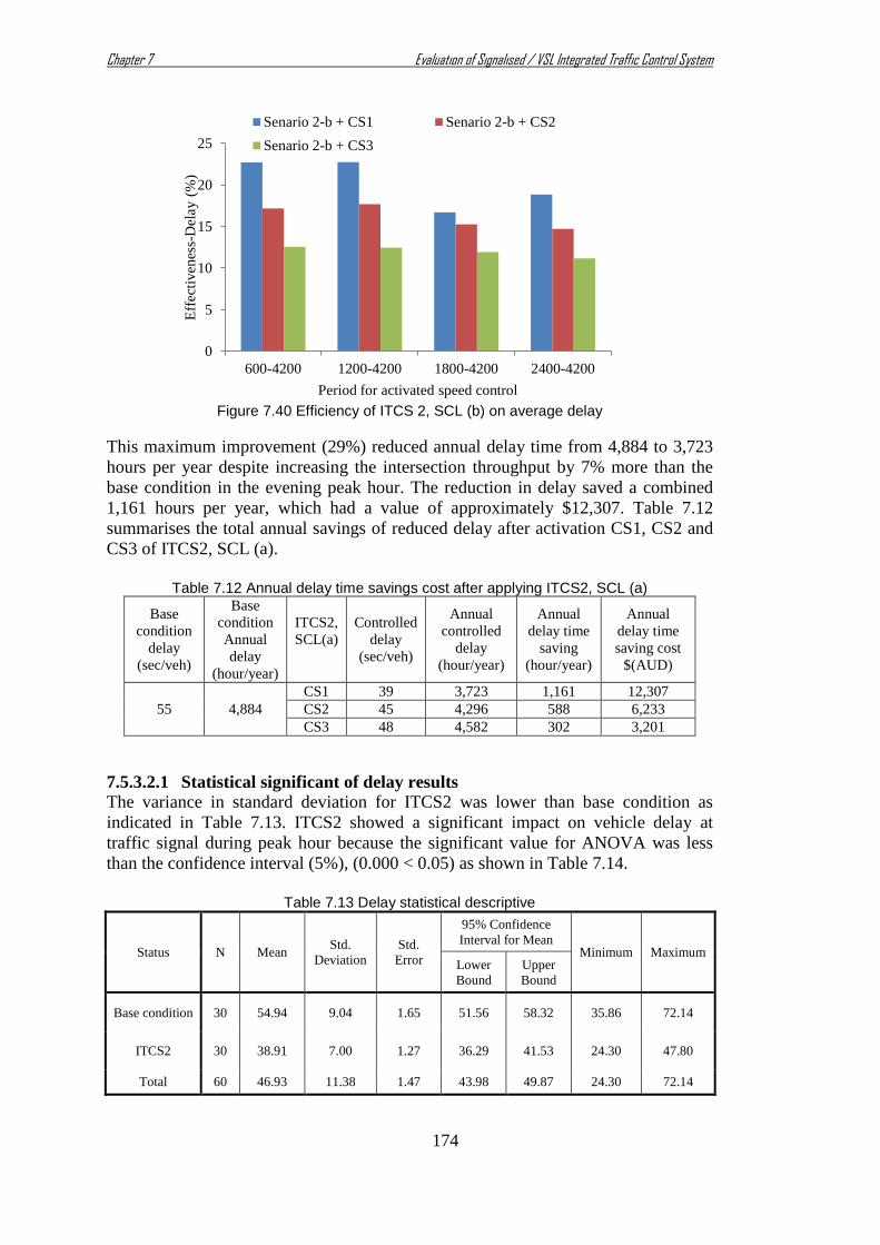
Chapter 7 Evaluation of Signalised / VSL Integrated Traffic Control System
174
Figure 7.40 Efficiency of ITCS 2, SCL (b) on average delay
This maximum improvement (29%) reduced annual delay time from 4,884 to 3,723
hours per year despite increasing the intersection throughput by 7% more than the
base condition in the evening peak hour. The reduction in delay saved a combined
1,161 hours per year, which had a value of approximately $12,307. Table 7.12
summarises the total annual savings of reduced delay after activation CS1, CS2 and
CS3 of ITCS2, SCL (a).
Table 7.12 Annual delay time savings cost after applying ITCS2, SCL (a)
Base
condition
delay
(sec/veh)
Base
condition
Annual
delay
(hour/year)
ITCS2,
SCL(a)
Controlled
delay
(sec/veh)
Annual
controlled
delay
(hour/year)
Annual
delay time
saving
(hour/year)
Annual
delay time
saving cost
$(AUD)
55
4,884
CS1 39 3,723 1,161 12,307
CS2 45 4,296 588 6,233
CS3 48 4,582 302 3,201
7.5.3.2.1 Statistical significant of delay results
The variance in standard deviation for ITCS2 was lower than base condition as
indicated in Table 7.13. ITCS2 showed a significant impact on vehicle delay at
traffic signal during peak hour because the significant value for ANOVA was less
than the confidence interval (5%), (0.000 < 0.05) as shown in Table 7.14.
Table 7.13 Delay statistical descriptive
Status N Mean Std.
Deviation
Std.
Error
95% Confidence
Interval for Mean Minimum Maximum
Lower
Bound
Upper
Bound
Base condition 30 54.94 9.04 1.65 51.56 58.32 35.86 72.14
ITCS2 30 38.91 7.00 1.27 36.29 41.53 24.30 47.80
Total 60 46.93 11.38 1.47 43.98 49.87 24.30 72.14
0
5
10
15
20
25
600-4200 1200-4200 1800-4200 2400-4200
Eff
ecti
ven
ess-
Del
ay (
%)
Period for activated speed control
Senario 2-b + CS1 Senario 2-b + CS2
Senario 2-b + CS3

Chapter 7 Evaluation of Signalised / VSL Integrated Traffic Control System
175
Table 7.14 Delay, One-Way ANOVA
Status Sum of Squares df Mean Square F Sig.
Between Groups 3856.08 1 3856.08 58.91 .000
Within Groups 3796.08 58 65.45
Total 7652.16 59
7.5.3.3 Evaluation of the variation in average stopped delay
Figure 7.41 and Figure 7.42 show the effect of ITCS 2 on average stopped delay at
intersection 2. The initial average stopped delay was 45 seconds. Similar to the
average delay indicator, stopped delay changed considerably by using SCL (a) of
ITCS 2. The average stopped delay declined from 45 seconds (non-control) to 31
seconds when SCL (a) was implemented at CS1 and launched 600s-4200s after at
the start of congestion and declined to 34 seconds when SCL (b) was implemented at
CS1 and launched at the same period.
The maximum reduction in stopped delay was achieved using SCL (a) because it
produced a reduced stopped delay. These results led to the conclusion that reducing
the speed limit increased arrival flow thereby the stopped delay was increased
accordingly. Positions CS2 and CS3 achieved a lower reduction than CS1 for the
average stopped parameter because they were located further away from the
downstream intersection. The main effect of ITCS 2 was due to the location of the
control speed zone and secondly due to the activation time period. Increasing the
speed control limits contributed to increasing the stopped delay because it increased
the number of vehicles and the queue length at the downstream intersection.
Figure 7.41 Average stopped delay before and after applying ITCS 2, SCL (a)
30
32
34
36
38
40
42
44
46
600-4200 1200-4200 1800-4200 2400-4200
Avea
ge
sto
pp
ed d
elay
(se
c/veh
)
Period for activated speed control
Senario 2-a + CS1 Senario 2-a + CS2
Senario 2-a + CS3 Base

Chapter 7 Evaluation of Signalised / VSL Integrated Traffic Control System
176
Figure 7.42 Average stopped delay before and after applying ITCS 2, SCL (b)
Figure 7.43 and Figure 7.44 show the effect of ITCS 2 on average stopped delay at
intersection 2. A maximum improvement of 30% was achieved by SCL (a). SCL (b)
achieved 24% improvement due to increasing the speed limit ranges from 30-35 to
40-45 km/hr.
Figure 7.43 Efficiency of ITCS 2, SCL (a) on average stopped delay
30
32
34
36
38
40
42
44
46
600-4200 1200-4200 1800-4200 2400-4200
Avea
ge
sto
pp
ed d
elay
(se
c/veh
)
Period for activated speed control
Senario 2-b + CS1 Senario 2-b + CS2
Senario 2-b + CS3 Base
0
5
10
15
20
25
30
35
600-4200 1200-4200 1800-4200 2400-4200
Eff
ecti
ven
ess-
Sto
pp
ed d
elay
(%
)
Period for activated speed control
Senario 2-a + CS1 Senario 2-a + CS2
Senario 2-a + CS3

Chapter 7 Evaluation of Signalised / VSL Integrated Traffic Control System
177
Figure 7.44 Efficiency of ITCS 2, SCL (b) on average stopped delay
7.5.3.4 Evaluation of the variation in average number of stops
Figure 7.45 and Figure 7.46 show the effect of ITCS 2 on the average number of
stops at intersection 2. The initial number of stops was 1.16 and this decreased
dramatically after applying SCL (a) and (b). Activating SCL (a) at CS1 decreased the
number of stops to 0.86 while activating SCL (b) at the same control speed location
reduced the number of stops to 0.95. The difference was caused by increasing the
speed control limits. Minimising the number and frequency of stops reduced the
acceleration and deceleration of vehicles which turn in reduced braking. These
factors assisted in improving the traffic safety in the vicinity of signalised
intersections during the congestion period. ITCS 2 improved this parameter more
than ITCS 1 due to the reduction in queue length at intersection 2. All sub-scenarios
of ITCS 2 showed a positive improvement in reducing the number of stops which
resulted in enhancing the traffic safety.
Figure 7.45 Average number of stops before and after applying ITCS 2, SCL (a)
0
5
10
15
20
25
30
600-4200 1200-4200 1800-4200 2400-4200
Eff
ecti
ven
ess-
Sto
pp
ed d
elay
(%
)
Period for activated speed control
Senario 2-b + CS1 Senario 2-b + CS2
Senario 2-b + CS3
0.8
0.85
0.9
0.95
1
1.05
1.1
1.15
1.2
600-4200 1200-4200 1800-4200 2400-4200
Aver
age
num
ber
of
sto
ps
Period for activated speed control
Senario 2-a + CS1 Senario 2-a + CS2
Senario 2-a + CS3 Base

Chapter 7 Evaluation of Signalised / VSL Integrated Traffic Control System
178
Figure 7.46 Average number of stops before and after applying ITCS 2, SCL (b)
Figure 7.47 and Figure 7.48 show the efficiency of ITCS 2 on the average number of
stops parameter at intersection 2. The maximum improvement was 27% due to SCL
(a) and approximately 19% due to apply SCL (b). Table 7.15 shows the effectiveness
of ITCS 2 on the performance of intersection 2 in terms of queue length, delay and
stopped delay, and number of stops. SCL (a) achieved the highest traffic
management efficiency at the intersection 2.
Figure 7.47 Efficiency of ITCS 2, SCL (a) on average number of stops
0.8
0.85
0.9
0.95
1
1.05
1.1
1.15
1.2
600-4200 1200-4200 1800-4200 2400-4200
Aver
age
num
ber
of
sto
ps
Period for activated speed control
Senario 2-b + CS1 Senario 2-b + CS2
Senario 2-b + CS3 Base
0
5
10
15
20
25
30
600-4200 1200-4200 1800-4200 2400-4200
Aver
age
num
ber
of
sto
ps
Eff
. %
Period for activated speed control
Senario 2-a + CS1 Senario 2-a + CS2Senario 2-a + CS3

Chapter 7 Evaluation of Signalised / VSL Integrated Traffic Control System
179
Figure 7.48 Efficiency of ITCS 2, SCL (b) on average number of stops
Table 7.15 Maximum efficiency of ITCS 2 for intersection parameters
Efficiency of
ITCS 2
Average
queue %
Average
delay %
Average
stopped delay %
Average number
of stops %
SCL (a) 28 29 30 27
SCL (b) 24 23 24 19
Evaluation of ITCS 2 on the performance of traffic flow 7.5.4parameters
In the following sections, macroscopic traffic flow characteristics of speed, flow and
density for the WB link at intersection 2 were estimated to investigate the effect of
ITCS 2 before and after applying ITCS2.
7.5.4.1 Evaluation the changes in average speed
Figure 7.49 and Figure 7.50 show the effect of ITCS 2 on average speed for SCL (a)
and (b) respectively. The initial speed was 39 km/hr and rose to 43 km/hr after
activating CS1 for SCL (a) for 600s-4200s. This produced only a small variation in
the speed profiles of all sub-scenarios. The flow was nearly constant and of a
uniform distribution because the analysis was carried out during the peak period.
Increasing the timing of the signal by 20s improved vehicles speed to 43 km/hr once
SCL (a) was implemented at CS1 and launched for 600s-4200s. The variation in
results for SCL (a) and SCL (b) was not significant (less than 1%) because both
SCLs only improved the speed of vehicles up to 43 km/hr.
0
2
4
6
8
10
12
14
16
18
20
600-4200 1200-4200 1800-4200 2400-4200
Aver
age
num
ber
of
sto
ps
Eff
. %
Period for activated speed control
Senario 2-b + CS1 Senario 2-b + CS2
Senario 2-b + CS3

Chapter 7 Evaluation of Signalised / VSL Integrated Traffic Control System
180
Figure 7.49 Average speed before and after applying ITCS 2, SCL (a)
Figure 7.50 Average speed before and after applying ITCS 2, SCL (b)
Figure 7.51 and Figure 7.52 show the improvement due to ITCS 2 on the average
speed for SCL (a) and (b) respectively. SCL (a) was approximately 8% to 11% better
while SCL (b) was approximately 8% to 10% better. This variation in improvement
was due to the difference in speed control range. In general, the improvement
increased from 8% to 9% for almost all control speed locations and for all speed
control periods. These results showed that using ITCS2 during the peak period
created a limited improvement in speed for all sub-scenarios.
36
37
38
39
40
41
42
43
44
600-4200 1200-4200 1800-4200 2400-4200
Aver
age
spee
d (
km
/hr)
Period for activated speed control
Scenario 2-a + CS1 Scenario 2-a + CS2
Scenario 2-a + CS3 Base (no-control)
36
37
38
39
40
41
42
43
44
600-4200 1200-4200 1800-4200 2400-4200
Aver
age
spee
d (
km
/hr)
Period for activated speed control
Scenario 2-b + CS1 Scenario 2-b + CS2
Scenario 2-b + CS3 Base (no-control)

Chapter 7 Evaluation of Signalised / VSL Integrated Traffic Control System
181
Figure 7.51 Efficiency of ITCS 2, SCL (a) on average speed
Figure 7.52 Efficiency of ITCS 2, SCL (b) on average speed
7.5.4.1.1 Evaluation of savings in crash costs on the GAR using ITCS2
ITCS2 reduced variation in the speed of vehicles travelling along the congested link.
This reduced the probability of fatality during the congestion period. Reducing speed
variation by 4.16 km/hr during congestion periods increased speed homogenity and
decreased the probability of fatality by 1.56%. Table 7.16 shows that the probability
of fatality for the current traffic situation decreased from 3.6% to 2.04% after
employing ITCS2 and improved the crash costs by 1.56%. Table 7.17 shows that if
ITCS2 was applied on the GAR, the total annual saving in fatality relate crash costs
would be $95,118.
Table 7.16 Probability of fatality at GAR before and after using ITCS2
Status Average speed
(km/hr)
Posted
speed
(km/hr)
Speed
deviation
(km/hr)
Probability of
Fatality*
(%)
Improve
(%)
Base
condition 39 70 31 3.6
1.56
ITCS2 43.16 70 26.84 2.04
Probability of fatality= (Speed devaition/71)4
0
2
4
6
8
10
12
600-4200 1200-4200 1800-4200 2400-4200
Eff
ecti
ven
ess-
Sp
eed
(%
)
Period for activated speed control
Scenario 2-a + CS1 Scenario 2-a + CS2
Scenario 2-a + CS3
7
7.5
8
8.5
9
9.5
10
600-4200 1200-4200 1800-4200 2400-4200
Eff
ecti
ven
ess-
Sp
eed
(%
)
Period for activated speed control
Scenario 2-b + CS1 Scenario 2-b + CS2
Scenario 2-b + CS3

Chapter 7 Evaluation of Signalised / VSL Integrated Traffic Control System
182
Table 7.17 Total annual savings in crash costs a GAR after applying ITCS2
Year Fatal Hospitalisation Medical treatment
& minor injury Property damage
2006 0 11 31 16
2007 1 14 19 9
2008 1 13 25 19
2009 1 14 27 17
2010 0 7 30 13
Average 0.6 11.8 26.4 14.8
Improve 1.56% 0.00936 0.18408 0.41184 0.23088
Cost/crash ($AUD) 3,083,000 307,500 17,000 11,500
Savings/year ($AUD) 28,857 56,605 7,001 2,655
Total annual savings ($AUD) 95,118
7.5.4.1.2 Statistical significant of speed results
The statistical variance of speed results under the base condition and ITCS2 were
non-significant for parts 1 and 2 as illustrated in Table 7.18 and Table 7.20. The
ITCS2 showed significant impact on vehicle speed results regardless of whether the
part was close to or away from the signalised intersection area. Table 7.19 and
Table 7.21 show that ITCS2 had a great significant impact on vehicle speed because
the significant value for ANOVA was less than the confidence interval (5%), (.000
<.05) for both parts.
Table 7.18 Speed statistical descriptive for part 1
Status N Mean Std.
Deviation
Std.
Error
95% Confidence
Interval for Mean Minimum Maximum
Lower
Bound
Upper
Bound
Base
condition 30 12.04 1.83 .33 11.36 12.73 8.90 16.35
ITCS2 30 15.88 3.17 .57 14.69 17.06 11.53 22.53
Total 60 13.96 3.21 .41 13.13 14.79 8.90 22.53
Table 7.19 Speed, One-Way ANOVA for part 1
Status Sum of Squares df Mean Square F Sig.
Between Groups 220.55 1 220.55 32.80 .000
Within Groups 389.95 58 6.72
Total 610.51 59

Chapter 7 Evaluation of Signalised / VSL Integrated Traffic Control System
183
Table 7.20 Speed statistical descriptive for part 2
Status N Mean Std.
Deviation
Std.
Error
95% Confidence
Interval for Mean Minimum Maximum
Lower
Bound
Upper
Bound
Base
condition 30 65.96 .89 .16 65.63 66.30 64.32 68.22
ITCS2 30 70.44 .72 .13 70.17 70.71 69.51 71.97
Total 60 68.20 2.39 .30 67.58 68.82 64.32 71.97
Table 7.21 Speed, One-Way ANOVA for part 2
Status Sum of Squares df Mean Square F Sig.
Between Groups 301.26 1 301.26 456.16 .000
Within Groups 38.30 58 .66
Total 339.57 59
7.5.4.2 Evaluation of the changes in flow
Figure 7.53 and Figure 7.54 show the effect of ITCS 2 on average flow for SCL (a)
and (b) respectively. The initial flow was 1332 veh/hr and this flow increased after
applying ITCS2. The variation in flow between all sub-scenarios was nearly constant
except for the flow produced by activating CS2 for SCL (a). The maximum flow
reached 1432 veh/hr for SCL (a) and (b). Changing the control speed locations did
not make a big difference in throughput at intersection 2 despite increasing the signal
timing for the WB lanes by 20 seconds. The reason was due to limited improvement
in the traffic density during the peak simulation period.
Figure 7.53 Average flow before and after applying ITCS 2, SCL (a)
1320
1340
1360
1380
1400
1420
1440
600-4200 1200-4200 1800-4200 2400-4200
Aver
age
flo
w (
veh
/hr)
Period for activated speed control
Scenario 2-a + CS1 Scenario 2-a + CS2
Scenario 2-a + CS3 Base (no-control)

Chapter 7 Evaluation of Signalised / VSL Integrated Traffic Control System
184
Figure 7.54 Average flow before and after applying ITCS 2, SCL (b)
Figure 7.55 and Figure 7.56 show the efficiency of ITCS 2 on average flow for SCL
(a) and (b) respectively. The efficiency of ITCS 2 was an almost constant 7% over
all sub-scenarios. By comparison with ITCS 2 and VSL applications, there were no
differences in the maximum efficiency of the flow between all traffic management
strategies. Scenario 2 (ITCS2) improved vehicle accessibility by about 24,000
vehicles per year. The improvement in vehicle accessibility was nearly constant for
VSL, ITCS1 and ITCS2 during the peak period.
Figure 7.55 Efficiency of ITCS 2, SCL (a) on average flow
1320
1340
1360
1380
1400
1420
1440
600-4200 1200-4200 1800-4200 2400-4200
Aver
age
flo
w (
veh
/hr)
Period for activated speed control
Scenario 2-b + CS1 Scenario 2-b + CS2
Scenario 2-b + CS3 Base (no-control)
0
1
2
3
4
5
6
7
8
600-4200 1200-4200 1800-4200 2400-4200
Eff
ecti
ven
ess-
Flo
w (
%)
Period for activated speed control
Scenario 2-a + CS1 Scenario 2-a + CS2
Scenario 2-a + CS3

Chapter 7 Evaluation of Signalised / VSL Integrated Traffic Control System
185
Figure 7.56 Efficiency of ITCS 2, SCL (b) on average flow
7.5.4.3 Evaluation of the changes in density
Figure 7.57 and Figure 7.58 show the effect of ITCS 2 on average density for SCL
(a) and (b) respectively. There was hardly small variation in traffic density before
and after using ITCS 2 due to a constant improvement in speed and flow. The initial
density was 34 veh/km which only dropped to 33 veh/km. This supported the finding
that ITCS was able to maintain the traffic density while maximising flow and speed
along the approach link at intersection 2.
Figure 7.57 Average density before and after applying ITCS 2, SCL (a)
6.2
6.4
6.6
6.8
7
7.2
7.4
7.6
600-4200 1200-4200 1800-4200 2400-4200
Eff
ecti
ven
ess-
Flo
w (
%)
Period for activated speed control
Scenario 2-b + CS1 Scenario 2-b + CS2
Scenario 2-b + CS3
32.2
32.4
32.6
32.8
33
33.2
33.4
33.6
33.8
34
34.2
34.4
600-4200 1200-4200 1800-4200 2400-4200
Aver
age
den
sity
(veh
/km
)
Period for activated speed control
Scenario 2-a + CS1 Scenario 2-a + CS2
Scenario 2-a + CS3 Base (no-control)

Chapter 7 Evaluation of Signalised / VSL Integrated Traffic Control System
186
Figure 7.58 Average density before and after applying ITCS 2, SCL (b)
Figure 7.59 and Figure 7.60 show the efficiency of ITCS 2 on average density for
SCL (a) and (b) respectively. The maximum efficiency was 3.5% for SCL (a) and
1% for SCL (b). The efficiency of SCL (b) was less than the efficiency of SCL (a)
because the speed control limits were changed from 30-35 km/hr to 40-45 km/hr.
This change increased the flow of vehicle arrivals and reduced the improvement due
to increased traffic density.
Figure 7.59 Efficiency of ITCS 2, SCL (a) on average density
33
33.2
33.4
33.6
33.8
34
34.2
34.4
600-4200 1200-4200 1800-4200 2400-4200
Aver
age
den
sity
(veh
/km
)
Period for activated speed control
Scenario 2-b + CS1 Scenario 2-b + CS2
Scenario 2-b + CS3 Base (no-control)
0
0.5
1
1.5
2
2.5
3
3.5
4
600-4200 1200-4200 1800-4200 2400-4200
Eff
ecti
ven
ess-
Den
sity
(%
)
Period for activated speed control
Scenario 2-a + CS1 Scenario 2-a + CS2
Scenario 2-a + CS3

Chapter 7 Evaluation of Signalised / VSL Integrated Traffic Control System
187
Figure 7.60 Efficiency of ITCS 2, SCL (b) on average density
Table 7.22 summarises the maximum efficiency of ITCS 2 on macroscopic traffic
flow parameters. The maximum improvement in speed was 10%, 7% for flow and
3.5 % for density. There is little difference between the data in Table 7.22 and
Table 7.11.
Table 7.22 Maximum efficiency of ITCS 2 regarding link parameters
Scenario 2
(ITCS2)
Maximum Efficiency %
Average speed Average flow Average density
SCL (a) 11 7 3.5
SCL (b) 9 7 2
Comparison of VSL applications and ITCS scenarios 7.6
This section discusses current (July 2013) traffic management on the GAR during
the evening peak period. A comparison was made between VSL alone and ITCS on
the flow situation to investigate which traffic management strategy was most
effective.
Four traffic parameters representing the main properties of the signalised
intersections were examined using both strategies. Both strategies produced
significant improvements in the performance of intersection 2 when contrasted with
baseline conditions during the congestion period. VSL achieved a 16% improvement
in average queue length while ITCS1 and ITCS2 achieved 20% and 28%
improvements respectively. ITCS1 produced a 4% increase over VSL and ITCS2
resulting in nearly double the improvement of VSL.
Both VSL and ITCS reduced the average delay at intersection 2. The average delay
was 55 seconds for the base line conditions and reduced to 46, 44.5 and 39 seconds
after applying VSL, ITCS1 and ITCS2 respectively. The LOS E for the baseline
condition improved to LOS D after implementing VSL and ITCS. The LOS D for
VSL control was similar to the LOS of ITCS despite there being 11 seconds
difference between both strategies. This was due to the standard specification for
motor vehicle LOS thresholds by TRB (2010). The maximum reduction in delay
time was 15% after using VSL control. After integrating VSL application, the
0
0.5
1
1.5
2
2.5
600-4200 1200-4200 1800-4200 2400-4200
Eff
ecti
ven
ess-
Den
sity
(%
)
Period for activated speed control
Scenario 2-b + CS1 Scenario 2-b + CS2
Scenario 2-b + CS3

Chapter 7 Evaluation of Signalised / VSL Integrated Traffic Control System
188
reduction in delay time increased to 19% and 29% after employing ITCS1 and
ITCS2 respectively.
All the proposed traffic management strategies were able to improve the level of
service at intersection 2 from LOS E to LOS D. Improving traffic conditions began
with the application of VSLs, continued with ITCS1, and reached a maximum
improvement with ITCS2. Figure 7.61 shows the variation in the percentage of
efficiency for three traffic scenarios, VSLs, ITCS1, and ITCS2 with four traffic
parameters at intersection 2. ITCS2 produced the highest improvement in traffic
management, ITCS1 produced the second most improvement, and VSLs produced
the third most improvement. This shows that, VSLs can produce high levels of
service at intersection 2 if they are combined with other traffic scenarios (ITCS 1 and
ITCS 2). Table 7.23 summarises the maximum improvements achieved by VSL and
ITCS strategies.
Figure 7.61 Optimum efficiency of various traffic scenarios
Table 7.23 Maximum improvement due to VSL application and ITCS
Intersection parameters % Efficiency
VSLs ITCS1 ITCS2
Average queue 16 20 28
Average delay 15 19 29
Average stopped delay 15 17 29
Average number of stops 18 21 27
The annual delay time for base conditions amounted to 4,884 hours computed in
evening peak hour. VSL, ITCS1 and ITCS2 reduced the annual delay time to 4,391,
4248 and 3,723 hours respectively despite the intersection throughput increasing
from 1,332 to 1,432 veh/hr. The reduction in delay by using VSL, ITCS1 and ITCS2
could save 493, 636 and 1,161 hours per year respectively for vehicles travelling on
the WB of intersection 2. Since the value of vehicle delay time in Brisbane during
peak hour is $10.6 (Booz, 2003) this amounts to a savings of approximately $5,226,
$6,742 and $12,307. Table 7.24 shows the annual savings by reducing delay time
after employing VSL and ITCS for all vehicles travelling on WB link of intersection
2.
0
5
10
15
20
25
30
VSLs ITCS 1 ITCS 2
% E
ffic
iency
Traffic scenario
Average queue
Average delay
Average sopped delay
Average number of stops

Chapter 7 Evaluation of Signalised / VSL Integrated Traffic Control System
189
Table 7.24 The annual savings in delay time for VSL and ITCS Base condition
Control
strategy
Max.
delay
reduction
(%)
Annual
delay time
saving
(hour)
Annual
delay time
savings
($AUD)
Annual
delay
time
(hour)
Annual
delay
time cost
($AUD)
Annual
delay time
(hour)
Annual
delay time
cost
($AUD)
4,884 51,770
VSL 15 4,391 46,545 493 5,226
ITCS1 19 4,248 45,029 636 6,742
ITCS2 29 3,723 39,464 1,161 12,307
In addition, all VSL ranges and ITCS scenarios enhanced traffic safety by reducing
the average number of stops and this reduced the likelihood of rear-end collisions.
The effect of these traffic management strategies varies from one scenario to
another. VSL reduced the average number of stops by 18% and this increased to
21% and 27% after applying ITCS1 and ITCS2 respectively.
The influence of applying VSL and ITCS on macroscopic traffic parameters (speed,
flow and density) for the congest link are shown in Table 7.25. All proposed
scenarios improved speed, flow and density by 3-11%. ITCS1 and ITCS2 did not
improve the performance parameters more than VSL except for the speed parameter
(11%) in the case of ITCS2. This was due to a small improvement in traffic density
(3.5%). This occurred because the link reached optimum capacity by using the VSL
strategy. It was also due to the traffic analysis being carried out during the peak hour
period. During this period, the space headways between vehicles were small, which
resulted in increasing the interaction between vehicles (high traffic density) thereby
constraining the speeds for vehicles.
Table 7.25 Maximum improvement regarding link parameters
Macroscopic parameters % Efficiency
VSLs ITCS1 ITCS2
Average speed 9 9 11
Average flow 7 7 7
Average density 3 3 3.5
ITCS was able to increase the efficiency of the signalised intersection but it was
unable to optimise the efficiency of macroscopic parameters beyond what was
achieved by VSL. Both VSL and ITCS increased flow by 7% and this indicated they
were able to increase mobility along the GAR during the peak hour and increase the
vehicle accessibility by about 24,000 vehicles per a year. Figure 7.62 shows a
constant improvement in efficiency for all proposed traffic scenarios at GAR for the
macroscopic parameters of speed, flow, and density.

Chapter 7 Evaluation of Signalised / VSL Integrated Traffic Control System
190
Figure 7.62 Maximum improvement at the approach link of intersection 2
Reducing the speed variations along the congested link during the peak hour reduced
the probability of fatality at the GAR. VSL and ITCS improve the risk of crashes at
the GAR by 1.35% and 1.56% respectively. These improvements decreased the total
annual costs to all crash types on the GAR and potentially saved around $82,000 and
$95,000 as shown in Table 7.26.
Table 7.26 Maximum expected annual saving from VSL and ITCS application
Status Improve
(%)
Annual saving in crash costs ($AUD) Total
annual
savings
($AUD) Fatal Hospitalisation
Medical
treatment &
minor
injury
Property
damage
VSL 1.35 24,972 48,985 6,059 2,298 82,314
ITCS1 1.30 24,047 47,171 5,834 2,213 79,265
ITCS2 1.56 28,857 56,605 7,001 2,655 95,118
The research investigated the effect of VSL and ITCS during peak hours on a
congested link in Brisbane city which is about 6.7 km long. The result from this
study was used to estimate the total saving from application of VSL and ITCS during
peak hours for Brisbane Metropolitan Area (BMA). The total length of arterial road
network in Brisbane is 469 km. Out of this, about 191 km (41%) of arterial roads are
congested (Department of Transport and Main Roads (TMR), 2010).
Table 7.27 shows that the total annual saving that can be expected from reducing
crashes in the congested arterials in Brisbane will be around $2,347,000, $2,260,000
and $ 2,712,000 due to the use of VSL, ITCS1 and ITCS2 respectively.
Table 7.27 Total annual savings in crashes for BMA
Severity of crash Annual saving in crash costs ($AUD)
VSL ITCS1 ITCS2
Fatal 711,888 685,519 822,640
Hospitalisation 1,396,438 1,344,726 1,613,665
Medical treatment & minor injury 172,727 166,313 199,581
Property damage 65,510 63,087 75,687
Total annual savings ($AUD 2,346,563 2,259,644 2,711,573
0
2
4
6
8
10
12
VSLs ITCS 1 ITCS 2
% E
ffic
iency
Traffic scenario
Average speed Average flow
Average density

Chapter 7 Evaluation of Signalised / VSL Integrated Traffic Control System
191
Influence of ITCS on total travel time 7.7
The effect of ITCS on total travel time (TTT) was investigated along the WB lanes
of GAR (6.7km). Speed control limits were used in evaluating total travel time. A
comparison between base line conditions (no-control) and ITCS scenarios was made
to find the effect of ITCS on total travel time.
Figure 7.63 shows that the base line conditions had higher TTT than all ITCS
scenarios. The base line total travel time was 598 seconds which reduced to 593,
572, 590, and 566 seconds by using ITCS 1 of SCL (a) and SCL (b), and ITCS 2 of
SCL (a) and SCL (b) respectively. SCL (a) of each scenario recorded a TTT higher
than SCL (b) because SCL (a) used a speed control limit of 30-35 km/hr and SCL (b)
used a speed control limit of 40-45 km/hr. SCL (a) achieved a high reduction in
delay and stopped delay at the signalised intersection but it achieved a smaller
reduction in TTT.
For example during the evening peak hour, the actual mean travel time for the WB
was 598 seconds with a total flow of 1,542 veh/hr. This TTT translated to 61,474
hours per a year which cost $651,629. ITCS2 generated 58,184 hours per year of
TTT for one peak hour simulation which cost $616,750. A maximum savings of 32
seconds, which is about 5.3% reduction in actual TTT, may firstly appear trivial, the
quantifiable benefits for a large volume of traffic can be substantial.
This 5.3% reduction in TTT amounted to 3,290 hours of travel time saved per year
for all vehicles traveling on WB direction in the evening peak hour. This produced a
savings of approximately $34,874. Table 7.28 indicates the variation in travel time
savings for VSL and ITCS.
Figure 7.63 Comparison between traffic base and ITCS scenarios regarding TTT
Table 7.28 Maximum expected annual saving in TTT along GAR
Base
condition
Annual delay
time
(hour/year)
Base
condition
Annual
TTT
$(AUD)
Control
strategy
% Max
TTT
reduction
Annual TTT
saving
(hours/year)
Annual TTT
saving cost
$(AD)
61,474 651,629
VSL 3.7 2,261 24,000
ITCS1 4.3 2,669 28,291
ITCS2 5.3 3,290 34,874
550
560
570
580
590
600
TT
T (
sec)
Base & ITCS scenarios

Chapter 7 Evaluation of Signalised / VSL Integrated Traffic Control System
192
The outcomes of VSL and ITCS throughput this research can be extended to
conclude all the congested arterials (191kms) in BMA. Table 7.29 shows that the
total annual saving that can be expected from reducing TTT in the congested
arterials in BMA will be around $696,000, $820,000 and $1,011,000 due to the use
of VSL, ITCS1 and ITCS2 respectively.
Table 7.29 Total annual savings in TTT for BMA
Traffic control strategy Annual TTT saving cost $(AD)
VSL 696,000
ITCS1 820,439
ITCS2 1,011,346
There is a trade-off in selecting the best ITCS scenario that can provide both high
performance and minimum TTT. Reducing speed limits can improve traffic
performance at signalised intersections but it also increases the TTT. Figure 7.64
shows that the maximum efficiency for ITCS scenarios for TTT was 5.3% and 4.3%
after using SCL (b) of ITCS2 and ITCS1 respectively. In contrast to VSL
applications, all ITCS scenarios achieved a positive reduction in TTT while some
VSLs scenarios increased TTT. ITCS minimised TTT by about 1.5% more than
VSLs.
Figure 7.64 Maximum efficiency of ITCS regarding TTT
Summary 7.8
This chapter investigated the efficiency of integrating two types of traffic control
systems, VSL applications and incremental changes to the cycle length of congested
traffic signals. The applications were tested for traffic management under two traffic
control scenarios on the GAR. Scenario 1 (ITCS1) was based on increasing the
signal timing for the WB lanes at intersections 1 and 2 by 10s, and managing the
upstream traffic with two speed control limits (SCLs), 30-35 km/hr and 40-45 km/hr
under different circumstances. Scenario 2 (ITCS2) was similar to Scenario 1 except
that the incremental increase in the signal timing was 20s.
Four traffic parameters covering the main performance properties of signalised
intersections were evaluated for the Integrated Traffic Control System (ITCS)
0
1
2
3
4
5
6
% E
ffic
iency
ITCS scenarios
TTT
Scenario 1-b Scenario 2-b Scenario 2-a Scenario 1-a

Chapter 7 Evaluation of Signalised / VSL Integrated Traffic Control System
193
scenarios. ITCS1 and ITCS2 improved the level of service at intersection 2 from
LOS E to LOS D despite there being a 5.5-second difference between both
strategies. This improvement in LOS enhanced the performance of the traffic signals
during the congestion period. The difference in results between ITCS1 and ITCS2
was due to the change in the signal timing. ITCS2 produced more improvement in all
signalised parameters than ITCS1. This means that VSL applications can produce
higher performance at intersection 2 when combined with other traffic scenarios
(ITCS1 and ITCS2).
A 20% improvement in average queue length, a 21% improvement in average
number of stops, a 19% improvement in average delay and 17% improvement in
average stopped delay were achieved by using ITCS1. A 28% improvement in
average queue length, a 27% improvement in average number of stops, a 29%
improvement in average delay and average stopped delay were achieved by using
ITCS2.
TTT decreased by 5.3% and 4.3% after employing ITCS1 and ITCS2. These results
reduced the cost of congestion by minimising the amount of delay and reducing the
travel time. At the same time, they improved the safety at traffic signals through
reducing rear-end collisions.
A maximum reduction in delay of 29% reduced the annual delay time from 4,884
hours to 3,723 hours despite increasing the intersection throughput by 7% in the
evening peak hour. The reduction in delay saved 1,161 hours per year, which valued
at approximately $12,307. This was more than twice the savings from using VSL.
A 27% reduction in the number of stops reduced the risk of rear-end collisions at
traffic signals. These results showed that using ITCS could enhance traffic safety in
the vicinity of intersection 2.
A constant increase in improvement was achieved for all proposed traffic scenarios
at GAR. All proposed scenarios improved speed, flow and density by 3-11%. ITCS1
and ITCS2 did not optimise the efficiency of link parameters more than the use of
VSL except for speed (11%) in the case of ITCS2. This was due to a small
improvement in traffic density (3.5%).
ITCS was able to increase the efficiency of the signalised intersection but it was
unable to optimise the efficiency of macroscopic parameters beyond what was
achieved by VSL. Both VSL and ITCS increased flow by 7% and this indicated they
were able to increase mobility along the GAR during the peak hour and increased the
annual vehicle accessibility by approximately 24,000 vehicles.
Due to the improvement in speed parameter from using ITCS, the probability of
fatality during the peak period was improved. A 9% decrease in speed variations
reduced the probability of fatality by approximately 1.35% while 11% enhancement
reduced the probability of fatality by around 1.56%. These improvements saved
annually $82,314-$95,118 in total estimated crash costs for the GAR during peak
hour.
The influence of the ITCS scenarios on TTT was investigated along the WB
direction of GAR. ITCS was able to reduce TTT by 5.3% at the most. For example,
during the evening peak hour, the actual mean travel time was 598 seconds for the
WB direction with total vehicle throughput of 1,542 veh/hr. This TTT translated to
61,474 hours per a year under uncontrolled conditions. A maximum saving of 32
seconds, which is about 5.3% reduction in actual vehicle travel time, may firstly
appear trivial at the high traffic volume but it can yield substantial benefits overall.
A savings of 58,184 hours per year was calculated from using ITCS for one peak
hour period. This 5.3% travel time savings translated to 3,290 hours of time saved

Chapter 7 Evaluation of Signalised / VSL Integrated Traffic Control System
194
per year for all vehicles traveling on the WB direction in the evening peak hour
which returned a TTT savings approximately $34,874.
The outcomes of VSL and ITCS can be extended to conclude the national level for
BMA in terms of crashes and TTT. The total estimated annual savings in crashes
was $2,347,000and $2,712,000 due to the use of VSL, and ITCS respectively. While
the total annual estimated savings in TTT was around $696,000 and $1,011,000.
All ITCS scenarios reduced TTT while some VSL scenarios increased TTT. ITCS
gave more than 1.5% improvement over VSL in TTT savings.
IBM SPSS proved that ITCS1 and ITCS2 had significant impact on vehicle delay
time at traffic signal and on vehicle speeds in a congested link regardless of whether
the link was close to or away from the intersection area.

CHAPTER EIGHT Summary and Conclusion
195
8 CHAPTER EIGHT Summary and Conclusion
Main conclusions from this study 8.1
The impact of VSL and ITCS on intersection parameters 8.1.1
The research investigated the application of Variable Speed limits (VSL) and its
incorporation into a new Integrated Traffic Control System (ITCS). Several traffic
control scenarios were used to estimate the effect of applying VSL control and ITCS.
The aim of the VSL control was to improve the level of service (LOS) and traffic
safety at downstream-signalised intersection. The key research outcomes were:
1. All VSL scenarios were useful for improving the traffic performance of
congested intersections from LOS E to LOS D.
2. VSL application improved the level of service during the peak hour by
reducing the overall delay and average stopped delay by approximately 15%.
3. VSL application improved the traffic safety during the peak hour by reducing
the average queue length and average number of stops by approximately
18%.
4. The position at which the speed control was implemented had a large impact
on the traffic performance of the downstream-congested intersections. VSLs
achieved greater efficiency the closer they were applied to the source of
congestion.
5. The efficiency of ITCS was based on the pre-emption time. The pre-emption
time for ITCS1 was small (10s) in contrast with ITCS2 where it was (20s).
The pre-emption times of ITCS1 and ITCS2 improved the level of service by
19% and 29% respectively. ITCS 2 was able to maximise the initial LOS to
the lower limit of LOS D and close to the upper limit of LOS C (35seconds).
6. ITCS1 and ITCS2 estimated the improvement of traffic safety by 21% and
27% respectively. VSLs applications can be more efficient when combined
with other traffic control strategies as shown for ITCS 1 and ITCS 2.
The impact of VSL and ITCS on macroscopic traffic 8.1.2characteristics
The effect of VSL and ITCS on macroscopic traffic characteristics (speed, flow, and
density) of a congested link were investigated for the peak traffic period. The same
signalised intersection scenarios were used in investigating the efficiency of both
VSL and ITCS. The aims of VSL control were to maximise the mobility (flow) and
travel speed, and to enhance or maintain the traffic density for the congested link
during the peak period. The aim of ITCS was to support the VSL operation during
the same peak period. The research outcomes were:
1. All scenarios of VSL and ITCS improve speed and flow and reduce density
by 3-9%.
2. ITCS1 and ITCS2 did not increase the efficiency of link parameters more
than the use of VSL except for speed (11%) in the case of ITCS2. This was

CHAPTER EIGHT Summary and Conclusion
196
due to only a small reduction in traffic density (3.5%) and the link reaching
its optimum capacity through the use of VSL (i.e. any other traffic scenario
could not improve this capacity).
3. ITCS increased the efficiency of the signalised intersection but it was not
able to maximise the efficiency of the link parameters more than the
efficiency achieved by VSL applications.
4. Both VSL and ITCS increased flow by 7% during the evening peak hour and
this indicated they were able to increase vehicle accessibility along the GAR
by 24,000 vehicles per year.
5. Statistical analysis showed that VSL and ITCS had a significant impact on
vehicle delay time at traffic signal and on vehicle speeds for a link close to or
away from the signalised intersection area during the peak hour.
The impact of VSL and ITCS on TTT 8.1.3
The third part of this work investigated the changes in total travel time (TTT) due to
VSL and ITCS. The TTT was considered for all west bound (WB) vehicles travelling
from intersection 6 to intersection 1. This is a distance of about 6.7 km. The
investigations lead to the following conclusions:
1. VSL and ITCS showed an acceptable reduction in TTT of 3.7% and 5.5%
respectively. Variation in improvements was due to different pre-emption
times for ITCS.
2. In comparison to VSL applications, all ITCS scenarios reduced TTT. Some
VSL scenarios increased TTT.
3. Overall, VSL and ITCS showed little impact on TTT due to the constrained
speed limits for non-congested links.
4. VSLs investigations on the east bound (EB) direction (Appendix B) showed
nearly the same positive results of WB direction for improving the
performance of intersection 6 and reducing TTT.
The impact of VSL and ITCS on annual savings 8.2
The research was able to estimate potential savings by using VSL and ITCS with
respect to congestion time savings and collision costs. The revenue was calculated
for one peak hour of control, with a five working day week. The vehicle delay time
value used for Brisbane during peak hour was $10.60 per hour (Booz, 2003).
1. The reduction in average delay time at WB of intersection 2 due to the use of
VSL, ITCS1 and ITCS2 was 493, 636 and 1,161 hours per year respectively.
This reduction in delay would save approximately $5,000, $7,000 and $12,000
respectively.
2. The reduction in TTT would be 2,261, 2,669 and 3,290 hours per year for all
vehicles traveling on WB direction of GAR due to the use of VSL, ITCS1 and
ITCS2 respectively. This would produce savings of approximately $24,000,
$28,000 and $35,000 respectively.
3. VSL application lowered the probability of fatalities along the congested link
by 1.35% while ITCS lowered the probability of fatality by 1.56%. These
improvements contributed significantly to reduce total estimated crash costs on
the GAR during peak hour of about $85,000 per year.

CHAPTER EIGHT Summary and Conclusion
197
4. Extrapolation shown that the total annual saving that can be expected from
reducing crashes in the congested arterials in Brisbane Metropolitan Area
(BMA) will be around $2,347,000, $2,260,000 and $2,712,000 due to the use
of VSL, ITCS1 and ITCS2 respectively. In addition to that, the total annual
savings estimated from decreasing TTT along the congested arterial roads in
BMA are about $696,000, $820,000 and $1,011,000 due to the use of VSL,
ITCS1 and ITCS2 respectively.
Summary 8.3
Urban traffic congestion is worsening globally with the ever-increasing urbanisation
and vehicle ownership. Long queues at intersections and blockage of traffic on urban
arterial roads have become routine during peak traffic hours and especially in the
vicinity of intersections. Traffic flow through signalised intersections and along
arterial roads is often interrupted and negatively affected by traffic congestion.
Congestion negatively influences people’s quality of life by increasing their travel
time, decreasing the performance of signalised intersection, decreasing mobility and
safety, increasing fuel consumption and contaminating the atmosphere, and creating
frustration.
Over the last three decades, the development of Intelligent Transport Systems (ITS)
has led to innovative new ways of managing and operating existing transportation
infrastructure. As part of ITS management strategies, Variable Speed Limits (VSL)
has been applied to improve the operation of congested motorways. Its application
has been intended to decrease the breakdown in traffic flow, reduce pollution and
increase the efficiency, reliability and safety of the road without needing major
physical changes to the road infrastructure. However, VSL does not appear to be
utilised to improve the operation of interrupted flow facilities such as occurs on
arterials, in terms of the level of service, safety and mobility.
Most of the control strategies that have been used to test the effectiveness of VSL
have been either theoretical studies or limited empirical evaluations. The number of
strategies required to validate efficiencies for a transportation system may be large
and field-testing would be prohibitively expensive. For this reason, microscopic
traffic simulation is a tool that is often used.
In this study VISSIM software was used to model a road network link and the
Griffith Arterial Road in Brisbane was selected as a case study area. The model used
data collected by the Queensland Department of Transport and Main Roads
(QDTMR) and data collected during the research by surveillance video cameras. The
model was developed to incorporate the road network and lane configurations, signal
timing and coordination, and vehicle and driver behaviour. One of the most difficult
tasks in the process was the calibration of saturation flow rate at each intersection to
represent actual conditions.
The GEH formula was employed to show the variation between the two sets of data,
field data and simulated result. One-Way ANOVA at 95% level of confidence was
applied to estimate the significant of employing VSL using IBM SPSS software.
The original hypothesis of the thesis was that VSL had potential to help alleviate
congestion and improve safety on urban arterial roads through its integration with
signalised control systems. The research has demonstrated through modelling using
the parameters obtained from QDTMR and extensive field work that VSL does have
great potential for traffic congestion relief on arterials and for associated savings
related to reduced travel time and crashes.

CHAPTER EIGHT Summary and Conclusion
198
Recommendations for future work 8.4
There is scope to extend the research finding to the arterial network level. Some of
the potential work possible to extend the research is outlined below:
1. VSL application can be employed in other Australian urbanised area and
other countries in order to mitigate traffic congestion.
2. This initial research on the application of VSL was undertaken for the peak
period. The impact of VSL on interrupted flow traffic performance during
off-peak periods could be investigated.
3. This investigation focused on WB and EB directional flows for GAR. The
research could be expanded to consider the effect of applying VSL on all four
directions of flow for intersections in the congested area.
4. VSL was combined with a single traffic control strategy (ITCS) in this study.
Further research could study the impact of VSL with other traffic control
strategies such as dynamic congestion pricing and adaptive control system.
5. The investigation did not consider the impact of VSL on public transport.
Further research could be undertaken to understand the impact of the
interaction between VSL and the efficiency of public transport.
6. The VSL application is implemented as a means of improving the traffic
conditions on urban arterial roads. The results indicate that VSL had a
significant impact on traffic conditions when drivers comply with variable
message signs. Further investigations may be needed to reveal the impact of
driver compliance on the effectiveness of VSL application.

References .
199
9 References
Abdel-Aty, M, Cunningham, RJ, Gayah, VV & Hsia, L 2008, Dynamic variable
speed limit strategies for real-time crash risk reduction on freeways,
Transportation Research Record, vol. 2078, pp. 108-116.
Abdy, ZR & Hellinga, BR 2008, Use of Microsimulation to Model Day-to-Day
Variability of Intersection Performance, Transportation Research Record,
vol. 2088, pp. 18-25.
Alessandri, A, di Febbraro, A, Ferrara, A & Punta, E 2002, Nonlinear optimization
for freeway control using variable-speed signaling, Vehicular Technology,
vol. 48, pp. 2042-2052.
Allaby, P, Hellinga, B & Bullock, M 2007, Variable speed limits: Safety and
operational impacts of a candidate control strategy for freeway applications,
Intelligent Transportation Systems, vol. 8, pp. 671-680.
Arnott, R, de Palma, A & Lindsey, R 1990, Departure time and route choice for the
morning commute, Transportation Research Part B, vol. 24, pp. 209-228.
Australian Bureau of Statistics (ABS) 2013, Survey of motor vehicle use, Canberra,
Australia.
Beckmann, M 1967, On Optimal Tolls for Highways, Tunnels, and Bridges
Proceedings of the Third International Symposium on the Theory of Traffic
Flow, New York, USA, pp. 331-341.
Bellemans, T, De Schutter, B & De Moor, B 2006, Model predictive control for
ramp metering of motorway traffic, Control Engineering Practice, vol. 14,
pp. 757-767.
Bertini, RL, Boice, S & Bogenberger, K 2006, Dynamics of variable speed limit
system surrounding bottleneck on german autobahn, Transportation
Research Record, vol. 1978, pp. 149-159.
Bloomberg, L & Dale, J 2000, Comparison of VISSIM and CORSIM traffic
simulation models on a congested network, Transportation Research Record,
vol. 1727, pp. 52-60.
Booz, AH 2003, Transport Demand Elasticities Study ACT, Canberra Department of
Urban Services.
Brust, H, Smolic, A, Mueller, K, Tech, G & Wiegand, T 2009, Mixed resolution
coding of stereoscopic video for mobile devices, The True Vision-Capture,
Transmission and Display of 3D Video, pp. 1-4.
Buchanan, C 1963, Traffic in towns, London UK, Penguin Books.

References .
200
Bureau of Transport and Regional Economics (BTRE) 2007, Estimating urban traffic
and congestion cost trends for Australian cities, Working Paper No.71.
Canberra, Australia.
Cairney, P 2013, Guide to Road Safety Part 1: Road Safety Overview, Australia,
Austroads, Sydney.
Carlson, RC, Papamichail, I, Papageorgiou, M & Messmer, A 2010, Optimal
motorway traffic flow control involving variable speed limits and ramp
metering, Transportation Science, vol. 44, pp. 238-253.
Catling, I 1977, A time-dependent approach to junction delays, Traffic Engineering
and Control, vol. 18, pp. 520-526.
Chen, C, Jia, Z & Varaiya, P 2001, Causes and cures of highway congestion, Control
Systems, vol. 21, pp. 26-32.
Chien, C, Zhang, Y & Ioannou, PA 1997, Traffic Density Control for Automated
Highway Systems, Automatica, vol. 33, pp. 1273-1285.
Chung, Y & Choi, K 2010, Dynamic Toll Concept to Assess Feasibility of High-
Occupancy Vehicle Lane on Kyungbu Freeway, South Korea, Transportation
Research Record, vol. 2178, pp. 162-169.
Coleman, J, Paniati, J, Cotton, R, Parker , M, Covey, R, Pena, H, Graham, D,
Robinson, M, MaClauley, J & Taylor, W 1996, FHWA study tour for speed
management and enforcement technology, US Department of Transportation,
Washington, DC.
Cronje, W 1983, Optimization model for isolated signalized traffic intersections,
Transportation Research Record, vol. 905, pp. 80-83.
Daganzo, CF 2007, Urban gridlock: macroscopic modeling and mitigation
approaches, Transportation Research Part B, vol. 41, pp. 49-62.
Dai, LL, Li, Y, Wang, YX & Liu, DB 2013, Application of Collaborative
Optimization Strategies for Traffic Control of Urban Arterial Intersection,
American Society of Civil Engineers, pp. 1031-1039.
Darma, Y, Karim, MR, Mohamad, J & Abdullah, S 2005, Control delay variability at
signalized intersection based on HCM method, Proceedings of the eastern
Asia society for Transportation Studies, vol. 5, pp. 945-958.
Department of Transport and Main Roads (TMR) 2010, South-east Queensland
travel time survey, TMR Modelling Data and Analysis Centre, Brisbane
QLD: http://www.tmr.qld.gov.au/Travel-and-transport/Road-and-traffic-
info/South-east-Queensland-travel-time-survey.aspx.

References .
201
Di Febbraro, A, Parisini, T, Sacone, S & Zoppoli, R 2001, Neural approximations
for feedback optimal control of freeway systems, Vehicular Technology, vol.
50, pp. 302-313.
Dion, F, Rakha, H & Kang, YS 2004, Comparison of delay estimates at under-
saturated and over-saturated pre-timed signalized intersections,
Transportation Research Part B, vol. 38, pp. 99-122.
Dowling, R 2007, Traffic Analysis Toolbox Volume VI: Definition, Interpretation,
and Calculation of Traffic Analysis Tools Measures of Effectiveness,
Washington, Department of Transportation Federal Highway Administration.
Factor, R, Prashker, JN & Mahalel, D 2012, The flashing green light paradox,
Transportation Research Part F, Traffic Psychology and Behaviour, vol. 15,
pp. 279-288.
Garber, NJ & Hoel, LA 2009, Traffic and Highway Engineering, USA, International
Thomson Publishing.
Geroliminis, N. 2007, Increasing mobility in cities by controlling overcrowding,
PhD thesis, University of California.
Geroliminis, N & Levinson, D 2009, Cordon pricing consistent with the physics of
overcrowding. In: H.K., W, Lam, SC & Wong, HKL (eds.), Transportation
and Traffic Theory 2009, Golden Jubilee, Netherland, Springer.
Gomes, G, May, A & Horowitz, R 2004, Congested freeway microsimulation model
using VISSIM, Transportation Research Record, vol. 1876, pp. 71-81.
Hadiuzzaman, M, Qiu, TZ & Lu, XY 2012, Variable Speed Limit Control Design for
Relieving Congestion Caused by Active Bottlenecks, Journal of
Transportation Engineering, vol. 139, pp. 358-370.
Hansen, M & Huang, Y 1997, Road supply and traffic in urban areas: a panel study,
Transportation Research A, vol. 31, pp. 205–218.
Harbord, B 1995, The application of SISTM to dynamic control on the
M25,Colloquium on Dynamic Control of Strategic Inter-Urban Road
Networks, London, UK The Institution of Engineering and Technology, pp.
1-5.
He, J & Hou, Z 2012, Ant colony algorithm for traffic signal timing optimization,
Advances in Engineering Software, vol. 43, pp. 14-18.
Hegyi, A, De Schutter, B & Hellendoorn, H 2005, Model predictive control for
optimal coordination of ramp metering and variable speed limits,
Transportation Research Part C, vol. 13, pp. 185-209.

References .
202
Hegyi, A, Schutter, BD & Hellendoorn, J 2003, Optimal coordination of variable
speed limits to suppress shock waves, Transportation Research Record, vol.
1852, pp. 167-174.
Herman, R & Ardekani, S 1984, Characterizing traffic conditions in urban areas,
Transportation Science, vol. 18, pp. 101-140.
Herman, R, Malakhoff, LA & Ardekani, SA 1988, Trip time-stop time studies of
extreme driver behaviors, Transportation Research Part A, vol. 22, pp. 427-
433.
Herman, R & Prigogine, I 1979, A two-fluid approach to town traffic, Science, vol.
204, pp. 148-151.
Hongfeng, C, Pu, X, Xiangzhao, F & Fen, L 2008, Public Attitudes Towards Policy
Instruments for Congestion Mitigation in Shanghai, Chinese Journal of
Population, vol. 6, pp. 40-47.
Hou, Z, Xu, J-X & Yan, J 2008, An iterative learning approach for density control of
freeway traffic flow via ramp metering, Transportation Research Part C, vol.
16, pp. 71-97.
Jin, S, Wang, D & Wang, L 2009, Traffic control strategy for a surface street on an
expressway-arterial corridor, Tsinghua Science & Technology, vol. 14, pp.
776-781.
Joksch, HC 1993, Velocity change and fatality risk in a crash: a rule of thumb,
Accident Analysis & Prevention, vol. 25, pp. 103-104.
Jones, B, Janssen, L & Mannering, F 1991, Analysis of the frequency and duration
of freeway accidents in Seattle, Accident Analysis & Prevention, vol. 23, pp.
239-255.
Jones, P 1995, Road pricing: The public viewpoint. In: Johansson, B & Mattson, L
(eds.), Road pricing: theory, empirical assessment and policy, Boston,
Kluwer.
Jonkers, E, Wilmink, I, Stoelhorst, H, Schreuder, M & Polderdijk, S 2011, Results of
field trials with dynamic speed limits in the Netherlands: improving
throughput and safety on the A12 freeway, Intelligent Transportation
Systems, Washington DC, USA, pp. 2168-2173.
Kejun, L, Meiping, Y, Jianlong, Z & Xiaoguang, Y 2008, Model predictive control
for variable speed limit in freeway work zone, Chinese Control Conference,
pp. 488-493.
Khattak, AJ 2001, Injury severity in multivehicle rear-end crashes, Transportation
Research Record, vol. 1746, pp. 59-68.

References .
203
Kohler, U 1974, Stability of vehicle platoons,Transportation and Traffic Theory,
University of New South Wales, Sydney, Australia Elsevier Publishing
Company, pp. 39-55.
Kotsialos, A, Papageorgiou, M, Diakaki, C, Pavlis, Y & Middelham, F 2002, Traffic
flow modeling of large-scale motorway networks using the macroscopic
modeling tool METANET, Intelligent Transportation Systems, vol. 3, pp.
282-292.
Kwon, E, Brannan, D, Shouman, K, Isackson, C & Arseneau, B 2007, Development
and Field Evaluation of Variable Advisory Speed Limit System for Work
Zones, Transportation Research Record, vol. 2015, pp. 12-18.
Laufer, J 2007, Freeway capacity, saturation flow and the car following behavioural
algorithm of the VISSIM microsimulation software,30th Australasian
Transport Research Forum, Melbourne, Australia, pp. 1-15.
Lee, C, Hellinga, B & Ozbay, K 2006, Quantifying effects of ramp metering on
freeway safety, Accident Analysis & Prevention, vol. 38, pp. 279-288.
Lenz, H, Sollacher, R & Lang, M 2001, Standing waves and the influence of speed
limits, space [km], vol. 518, pp. 1-5.
Levinson, D, Zhang, L, Das, S & Sheikh, A 2004, Measuring the Equity and
Efficiency of Ramp Meters, Minnesota: University of Minnesota, Department
of Civil Engineering.
Lin, P, Kang, K & Chang, G 2004, Exploring the effectiveness of variable speed
limit controls on highway work-zone operations, Journal of Intelligent
Transportation Systems, vol. 8, pp. 155-168.
Lownes, NE & Machemehl, RB 2006, VISSIM: a multi-parameter sensitivity
analysis, Simulation Conference, pp. 1406-1413.
Luk, J & Hepburn, S 1993, New review of Australian travel demand elasticities,
Victoria, Australia, Australian Road Research Board.
Luttinen, RT & Nevala, R 2002, Capacity and level of service of Finnish signalised
intersections, Helsinki, Finnish Road Administration.
Mahmassani, HS, Williams, J & Herman, R 1987, Performance of urban traffic
networks, The Tenth International on Transportation and Traffic Theory
Symposium, Cambridge, Massachusetts, Elsevier, pp. 78-88.
Marchand, M 1968, A note on optimal tolls in an imperfect environment,
Econometrica: Journal of the Econometric Society, vol. 36, pp. 575-581.
May, AD 1986, Traffic restraint: a review of the alternatives, Transportation
Research Part A, vol. 20, pp. 109-121.

References .
204
McDonald, JF 1995, Urban highway congestion, Transportation, vol. 22, pp. 353-
369.
Mogridge, MJH 1997, The self-defeating nature of urban road capacity policy : A
review of theories, disputes and available evidence, Transport Policy, vol. 4,
pp. 5-23.
O'Day, J & Flora, J 1982, Alternative measures of restraint system effectiveness:
interaction with crash severity factors, Society of Automotive Engineers,
Warrendale, pp. 1-6.
Ogden, KW & Newstead, SV 1994, Analysis of crash patterns at Victorian
signalised intersections: Monash University, Accident Research Centre.
Oketch, T & Carrick, M 2005, Calibration and validation of a micro-simulation
model in network analysis, Proceedings of the 84th
TRB Annual Meeting,
Washington DC, pp. 1-17.
Olszewski, P 1993, Overall delay, stopped delay, and stops at signalized
intersections, Journal of transportation engineering, vol. 119, pp. 835-852.
Olszewski, P & Xie, L 2005, Modelling the effects of road pricing on traffic in
Singapore, Transportation Research Part A, vol. 39, pp. 755-772.
Orski, C 1972, Car-Free Zones and Traffic Restraints: Tools of Environmental
Management, Highway Research Record, vol. 406, pp. 37-46.
Papageorgiou, M 1983, Applications of automatic control concepts to traffic flow
modeling and control, New York, Springer-Verlag.
Papageorgiou, M, Kosmatopoulos, E & Papamichail, I 2008, Effects of variable
speed limits on motorway traffic flow, Transportation Research Record, vol.
2047, pp. 37-48.
Papageorgiou, M & Kotsialos, A 2000, Freeway ramp metering: An overview,
Intelligent Transportation Systems, Dearborn, pp. 228-239.
Papamichail, I, Kotsialos, A, Margonis, I & Papageorgiou, M 2010, Coordinated
ramp metering for freeway networks–A model-predictive hierarchical control
approach, Transportation Research Part C, vol. 18, pp. 311-331.
Parthasarathi, P, Levinson, D & Karamalaputi, R 2003, Induced demand: a
microscopic perspective, Urban Studies, vol. 40, pp. 1335.
Pigou, A 1912, Wealth and Welfare, London: Macmillan.
Planning Transport Verkekr (PTV) AG 2011, User’s Manual, 5.3, Karlsruhe,
Germany.

References .
205
Rathi, A & Lieberman, E 1989, Effectiveness of traffic restraint for a congested
urban network: A simulation study, Urban Traffic Systems and Operations,
vol. 1232, pp. 95-102.
Retting, R & Cheung, I 2008, Traffic speeds associated with implementation of 80
mph speed limits on West Texas rural interstates, Journal of Safety Research,
vol. 39, pp. 529-534.
Rodegerdts, LA, Nevers, B, Robinson, B, Ringert, J, Koonce, P, Bansen, J, Nguyen,
T, McGill, J, Stewart, D & Suggett, J 2004, Signalized intersections:
informational guide, USA: Federal Highway Administration.
Roess, RP, Prassas, ES & McShane, WR 2004, Traffic engineering, Pearson/Prentice
Hall.
Sadek, AW & Smith, MC 2006, Challenges Calibrating Large-Scale Microscopic
Simulation Model of Diverse Urban, Suburban, and Rural Network: Practical
Guide, Transportation Research Board 85th
Annual Meeting, Washington
DC, pp. 1-19.
Smeed, R 1966, Road capacity of city centers, Traffic Engineering and Control, vol.
8, pp. 455-458.
Smulders, S 1992, Control by variable speed signs: The Dutch Experiment,
International Conference on Road Traffic Monitoring and Control London,
Institution of Electrical Engineers, pp. 99-103.
Stevanovic, A, Stevanovic, J & Kergaye, C 2013, Optimization of traffic signal
timings based on surrogate measures of safety, Transportation Research Part
C, vol. 32, pp. 159-178.
Sugiyama, N & Nagatani, T 2012, Multiple-vehicle collision induced by a sudden
stop in traffic flow, Physics Letters A, vol. 376, pp. 1803-1806.
Teply, S, Allingham, D, Richardson, D & Stephenson, B 1995, Canadian capacity
guide for signalized intersections, Canada, Institute of Transportation
Engineers.
Thomson, J 1967, Speeds and Flows of Traffic in Central London, Traffic
Engineering and Control, vol. 8, pp. 721–725.
Transport For London (TFL) 2004, Congestion Charging Central London-Impacts
Monitoring, Second Annual Report. London:
www.tfl.gov.uk/tfl/cclondon/ccmonitoring-2nd-report.shtml.
Transportation Research Board (TRB) 1985, Highway Capacity Manual 1985,
National Research Council, Washington DC.
Transportation Research Board (TRB) 2000, Highway Capacity Manual 2000,
National Research Council, Washington DC.

References .
206
Transportation Research Board (TRB) 2010, Highway Capacity Manual 2010,
National Research Council, Washington DC.
Troutbeck, R, Su, M & Luk, J 2007, National Performance Indicators for Network
Operations, Sydney, Australia.
Turner, S, Turner, B & Wood, G 2008, Accident prediction models for traffic
signals,ARRB Conference, Adelaide, South Australia, Australia, pp. 1-15.
Van Aerde, M & Rakha, H 2007, INTEGRATION © Release 2.30 for Windows:
User's Guide Volume I: Fundamental Model Features, Van Aerde & Assoc.,
Ltd., Blacksburg.
Verhoef, E, Nijkamp, P & Rietveld, P 1997, The social feasibility of road pricing: a
case study for the Randstad area, Journal of Transport Economics and
Policy, vol. 31, pp. 255-276.
Vickrey, W 1963, Pricing and Resource Allocation in Transportation and Public
Utilities: Pricing in Urban and Suburban Transport, American Economic
Review, vol. 53, pp. 452-465.
Viegas, JM 2001, Making urban road pricing acceptable and effective: searching for
quality and equity in urban mobility, Transport Policy, vol. 8, pp. 289-294.
Wang, Y, Papageorgiou, M, Sarros, G & Knibbe, WJ 2006, Feedback route guidance
applied to a large-scale express ring road, Transportation Research Record,
vol. 1965, pp. 79-88.
Wardrop, J 1953, Some theoretical aspects of road traffic research, vol. 4, pp. 72-73.
Watson, P & Holland, E 1978, Relieving traffic congestion: the Singapore area
license scheme, Staff Working Paper No. 281, Washington DC, World Bank.
Webster, FV 1958, Traffic signal settings, Road Research Laboratory, London:
Road Res, Tech.
Webster, FV & Cobbe, BM 1966, Traffic signals, London, Her Majestyás Stationery
Office.
Wiedemann, R & Reiter, U 1992, Microscopic traffic simulation: the simulation
system MISSION, background and actual state, Project ICARUS (V1052)
Final Report, Brussels, vol. 2, pp. 1-15.
Wiles, PB, Cooner, SA, Rathod, Y & Wallace, DG 2005, Advance Warning of
Stopped Traffic on Freeways: Field Studies of Congestion Warning Signs,
Austin, Texas Transportation Institute.

References .
207
Wu, Z, Sharma, A, Mannering, FL & Wang, S 2013, Safety impacts of signal-
warning flashers and speed control at high-speed signalized intersections,
Accident Analysis & Prevention, vol. 54, pp. 90-98.
Yan, X, Radwan, E & Abdel-Aty, M 2005, Characteristics of rear-end accidents at
signalized intersections using multiple logistic regression model, Accident
Analysis & Prevention, vol. 37, pp. 983-995.
Yang, Q, Han, LD & Cherry, CR 2013, Some measures for sustaining red-light
camera programs and their negative impacts, Transport Policy, vol. 29, pp.
192-198.
Zackor, H 1979, Self-sufficient control of speed on freeways, International
Symposium on Traffic Control Systems, vol. 2, pp. 226-249.
Zackor, H 1991, Speed limitation on freeways: Traffic-responsive strategies:
Pergamon Press, Oxford, United Kingdom.
Zahavi, Y 1972, Traffic performance evaluation of road networks by the α-
relationship, Traffic Engineering and Control, vol. 14, pp. 228-231.
Zhang, X & Yang, H 2004, The optimal cordon-based network congestion pricing
problem, Transportation Research Part B, vol. 38, pp. 517-537.
Zhou, S, Sun, J, Li, K & Yang, X 2013, Development of a Root Cause Degree
Procedure for measuring intersection safety factors, Safety Science, vol. 51,
pp. 257-266.

References .
208

APPENDIX A .
209
A. APPENDIX A
A.1 Development of VISSIM modelling
The aim of VISSIM modelling is to investigate the traffic problems of the GAR and
test proposed traffic management strategies that could relieve and mitigate flow at
congested intersections. In order to build a microscopic simulation model for GAR,
three types of data are required; physical design of the road network, definition of
vehicle characteristics, and knowledge of driver behaviour. In the present study, the
first two data sets are kept constant during the model building. The third category of
data is varied where it is necessary to replicate the actual traffic conditions along the
network.
A.1.1 Physical road network & traffic signal timing
The first step in constructing a VISSIM model is drawing the geometric design of
the study area. This was done using the VISSIM interface screen. An accurate and
easy way to obtain the layout of the network is by utilising Google-Earth, where an
unscaled aerial image can be taken of the selected study area and saved in the same
directory as the VISSIM files. Secondly, the image is uploaded as a background
screen for the VISSIM window. Thirdly, the image is scaled by following VISSIM
guidelines to match the actual measurements. Eventually, the scaled map is saved in
the same directory as the VISSIM files to avoid repeating the steps (more details can
be found in the VISSIM (2011). Figure A.1 depicts the aerial image layout of the
study area. The geometric design of the whole network, including lane
configurations and intersection locations, are setup by tracing the image background
using VISSIM links and connectors. The lane width of roadways can be obtained
from the aerial image using the Google-Earth toolbox or from field measurements.
Figure A.1 VISSIM background image of the study area
Intersection 2
Intersection 1 Intersection 3
Intersection 4
Intersection 5
Intersection 6

APPENDIX A .
210
Links area segments of any selected length of uniform roadway (same number of
lanes of the same width. Connectors are used to join segments. The following points
should be considered when creating VISSIM links and connectors:
1. Link type: By default, links have four driving behaviour classifications (urban,
freeway, footpath, or cycle path) and one of these behaviours should be assigned
to each link. Since the study area is focused on an urban area, the links were
allocated as urban (Wiedemann 1974). In addition, the number of lanes and their
width should be defined during the link design stage.
2. The lane change distance and the emergency stop distance needs to be defined for
each connector. In order to replicate actual traffic flow, appropriate distances are
used to control the traffic flow and the capacity of intersections.
3. Priority is assigned for merging lanes and for permitted signal operations.
4. Areas of reduced speed are modelled for the left and right turn movements at each
intersection as well as for curves along the road network.
5. Options for conflict areas can also be assigned at intersections to avoid blocking
by vehicles when an oversaturated condition occurs.
The next stage, after modelling the road network, is modelling the traffic signals. Six
isolated signalised intersections were created using the traffic control signal and
signal head tool. Since the research was focused only on the congested period, the
traffic signal behaviour was fairly close to a fixed timing plan. The signal timing
information and the traffic phase configuration were collected from the surveillance
videos taken along the studied area. In VISSIM, signalized intersections can be
created in different ways such as by built-in fixed-time control including the VISSIG
add-on or by using various external signal control logic add-on software such as
Econolite ASC/3, LISA+OMTC, SCATS, COOT, Vehicle-Actuated Signal Control
(VAP) , and Ring Barrier Controller (RBC). Based on the selected control logic,
VISSIM can simulate up to 125 signal groups per signal controller. It can also
distinguish between signal groups and signal heads.
In VISSIM, a signal group is associated with each signal head that belong to an
external control signal. All signal heads of the same group exhibit the same signal
status at all times. For the present study, a separate signal group was formed for each
individual signal head, in order to control the flow at each intersection. Signal heads
were created for each travel lane at the location of the signal stop line. The signal
group identifies the flow direction at each intersection (e.g., through movement, left
and right turn). Sometimes one signal group shared more than one signal head if they
have the same traffic characteristics in the same signal control. This occurs when two
lanes had the same flow directions (two through lanes). In order to create the signal-
timing plan, details about the cycle length and offset for each signal control need to
be entered in the signal program. Information about how long each signal group is
green, red, amber, and all red should be allocated via the signal program window.
The cycle length and the offset time is also entered in his window. Figure A.2
illustrates the signal control window for intersection 1.
Some of the traffic movements have special traffic phases such as permitted or
protected-permitted right turn. Since a pre-timed signal system doesn’t have this
operation, signal priority with signal head is used to imply the extra options in a
fixed timing plan.

APPENDIX A .
211
Figure A.2 Signal control window for intersection 1
A.1.2 Coding traffic data
Traffic volume, vehicle composition, desired speed and vehicle distribution
parameters are required for model simulation. Traffic flow can be inserted as a time
flow series. Observed hourly volume was used in VISSIM for each entrance point in
the network. Also, a warm-up period of 600 sec was considered for simulation
execution to fill the network with vehicles. the results for this period were excluded
from the analysis. VISSIM has the ability to model a variety of vehicle types that
reflect the diversity of vehicles in practice. Vehicle composition comprises a list of
one or more vehicle types. A flow percentage and a speed distribution are assigned
to each of these vehicle types. Four different vehicle types were modelled to reflect
the actual traffic compositions in the present study. Cars, trucks, buses and
motorcycles represent the mix of vehicles observed in practice and executed in
VISSIM. The first two types comprise the major input flow in creating the model
whereas buses and motorcycles represent minor input flows because their numbers
were very small during the survey period. The default characteristics contained in
VISSIM for each vehicle type are:
1. Static parameter: this section identifies the length, width and occupancy of
each vehicle type where the user is able to adjust the relative values except the
vehicle’s length which is considered constant. The present study used VISSIM
default static parameter values. Figure A.3 illustrates the vehicle type
classifications for the selected area.

APPENDIX A .
212
Figure A.3 VISSIM snapshot for such vehicle type
2. Function characteristics: In this section, minimum and maximum
acceleration and deceleration for each type of vehicle can be assigned and
adjusted to reflect the actual behaviour of drivers. VISSIM has default values for
each function and this option was used in the current study. Figure A.4 (a) and (b)
shows the deceleration and acceleration properties for car vehicle type.
(a) (b)
Figure A.4 Acceleration and deceleration functions
3. Vehicle distribution: This parameter defines the speed distribution, weight
and power of each type of vehicle. The user also can adjust these values and insert
new values. In the current study, the default values for the weight and power
distribution remained invariant. Since there are different link speeds along the
road network, various speed distributions were created based on each link speed
value. The actual desired speeds are varied from 60 km/h to 80 km/hr. Since the
most urbanised links are equipped with speed cameras, drivers may be more
compliant with the speed limit in these links. Because drivers are used to driving
5 to 10 km/h less than the actual speed in urban area, the desired speed
distribution was based on these thresholds.

APPENDIX A .
213
For example, if the speed limit was 80 km/h for such a link, the desired speed
distribution was set from 70 to 80 km/h.
The vehicle inputs from the previous step were used to spread traffic out along the
road network. In VISSIM, a route represents the path of vehicles through a group of
links and connectors. Route decisions can be assigned via two options, a static route
and a dynamic assignment route. Static assignment routes are required for at least
two points, the start point and the finish point at which the flow percentage or exact
volume can be identified for each defined destination. Sometimes, one point route
decision has more than one route destination, resembling a tree with several
branches.
Dynamic assignment routes include multiple origin-destination matrices based on an
iterative process. In this case, the drivers select their routes according to the travel
cost among a group of route destinations for several simulations, not only for one
simulation. The present study used the static assignment route to distribute the traffic
flow along the study area.
When it starts, the static route generates a defined route decision point which is
placed at the start of the origin link for the route. Then each route decision must be
followed by at least one defined destination during the simulation process. Simulated
time can be allocated and vehicle classes can be assigned for each signal route
decision. Figure A.5 shows an example of the static route created at the NB lane for
Beatty intersection.
Figure A.5 Static routes distributions
A.1.3 Driving behaviour
The concept of “car following” and the “lane change” models in VISSIM are set for
two types of driving behaviour based on Wiedeman 1974 and 1999. The first model
defines traffic flow behaviour in urban area whereas the second model defines traffic
flow on freeways. The study utilised the patterns defined by Wiedeman 1974
because they matched the driving behaviour observed in the study area. In VISSIM a
wide range of parameters can be used to set up both the “car following” and “lane
change” models.

APPENDIX A .
214
Some of these may be modified by experienced users to change the basic rules of
driver behaviour. Modified parameters drastically affect vehicle interactions, which
in turn changes the simulation results. Driving behaviour can be selected through
selection of the type of link behaviour. By default, five link types are predefined.
There are four behaviour sub categories influencing the psychophysical “car-
following” model. These are; following behaviour, lane change behaviour, lateral
behaviour, and signal control behaviour. Each sub-category is associated with a set
of parameters that controls the driving of the simulated vehicles along the road
network. There is no correlation expected between vehicle type and driver
behaviour.
In some cases, the initial execution of the model may exhibit correct traffic
movement along the road network but not necessarily reflect the correct real
measurements such as the number of vehicles for each lane at signalised
intersections and the intersection throughput. The first execution of the model aims
to determine the preliminary performance level that enables the user to understand
whether the model matches the observed data or needs further calibration of the
current driving behaviour parameter sets.
For study purposes, the car following behaviour, lane change parameters and signal
control behaviour were considered so as to model an exclusive interrupted flow.
A.1.3.1 The car following behaviour
The default parameters did not match the field volume distribution along the network
and did not reflect the discharged traffic movements (through, left and right
movements) at signalised intersections. This section will be governed by a set of
parameters that organise the flow of vehicles across the road network. These are:
1. Look ahead distance: This defines the distance that a driver can see forward
in order to react to other vehicles, either in front or to his side (within the same
link). The minimum default value is set to zero whereas the maximum value can
be 250 m. The study used the default setting.
2. Observed vehicle: This factor affects how well drivers in the network can
predict other vehicle’s movements and react accordingly. By default, four
vehicles are set to influence this element. The study used two observed vehicles in
order to increase the possibility of lane change and to speed up the simulation run.
Selecting higher values for this factor may slow down the simulation run and
reduce the possibility of changing lane particularly when the traffic volume is
high.
3. Look back distance: This defines the distance that a driver can see
backwards in order to react to other drivers behind him (within the same link).
The minimum default value is set to zero whereas the maximum value is set to
150 m. The study used the default settings.
4. Average standstill distance (ax): This represents the average desired
distance between stopped cars with a variation of ± 1 m and normal distribution
around 0.0 m with a standard deviation of 0.3 m.
5. Safety distance: It is the distance between two vehicles traversing through
the link .The additive part of the desired safety distance (bx_add) is set to 2 m, the
multiplicative part of desired safety distance (bx_mult) is set to 3 m, and both
affect the computation of the safety distance as shown in the following formula.

APPENDIX A .
215
A.1
where (d ) is the standstill distance and
( ) √ A.2
where
v: is the vehicle speed [m/s]
z:is a value of range [0,1] which is normal distributed around 0.5 with a
standard deviation of 0.15.
These parameters have a major influence on the safety distance and thus affect the
saturation flow rate. By changing the default parameters, various saturation flows
can be produced. In the present study, the default parameters were decreased to
match the actual field capacity. Defining the saturation flow in VISSIM is not
governed by a single value but rather it requires testing a set of driving behaviour
parameters that yield the actual saturation flow. This step is done by trial and error.
Since each link has its own geometric design and its own traffic characteristics,
several types of links were created to replicate real behaviour over the study area as
shown in Figure A.6.
Figure A.6 Links behaviour
A.1.3.2 The lane change parameters
In VISSIM 2011, there are two types of lane change setting and each type is
governed by a set of parameters:
1. Necessary lane change (in order to reach the next connector of a route): This
parameter is explained in the previous section and is mainly based on the
maximum acceptable deceleration for the leading vehicle and the trailing
vehicle on the new lane. It depends on the distance to the emergency stop
position of the next connector of the route. The present study used the
VISSIM default values for acceptable deceleration to change lanes. The other
two parameters (look back distance and emergency stop distance) that define
the connector properties were changed to match the habits of the drivers in

APPENDIX A .
216
the study area. The default, “look back distance” is 200 m but the study used
a higher distance, primarily to capture the actual driver behaviour. Since the
study was conducted during a congested period, it meant the road network
was under high traffic demand, and the drivers were not able to change lanes
within 200 m. Therefore, they were stopped at the emergency stop distance
waiting for an opportunity to change lanes. The reasons could be that the
spaces between vehicles was insufficient due to the high traffic volume, the
distance between two successive signals being short, and the proportion of
vehicles wanting to turn left/right being large. The initial simulation using the
default values yielded a lot of vehicles trying to change lanes within the
signalised area. This impedes the upstream flow and reduces the overall
traffic flow performance which in turn leads to creating unrealistic traffic
behaviour.
In order to overcome this situation the emergency stopping distance was increased to
prevent vehicles interacting downstream of signalised intersections. The solution was
successful where there was low traffic demand, a long distance between signals and
a low percentage of turning vehicles. The second most popular solution which is
used, is to increase the look back distance. Large distances lead to unrealistic
interactions between vehicles far from the signal area. The study used different
values in order to adjust the look back distances individually for each link allowing
vehicles sufficient space to change lanes. Table A.1 shows a list of adjusted look-
back distances for the mainstream links.
Table A.1 Modified look back distances for EB direction
Intersection
No. Direction
TH
look-back
RT
look-back
LT
look-back
1 EB 350 400 600
2 EB 250 1000 250
3 EB 600 1500 -
4 EB 250 250 500
5 EB 250 1600 1200
6 EB 800 1500 1500
2. Free lane change: This parameter allowed vehicles to overtake in any travel
lane. VISSIM periodically checks the desired safety distance for the vehicles
intending to change lanes based on their speed and the speed of the trailing
vehicle in the new lane. In addition to the parameters above, there are some
other parameters that influence on the decision to change lanes which are:
a. Waiting time before diffusion: This defines the maximum amount
of time a vehicle can wait at the emergency stop position waiting for a gap
to change lanes in order to stay in its route. Vehicles that not able to change
lanes within this period will disappear from the network (diffusion) and an
error file will be written explaining the time and location of the removal.
The default value is 60s. The study used values of 20-40s instead of the
default value for some mainstream links. This setting was adjusted to
minimise the waiting time for vehicles stopped at emergency stop locations
so as to reduce obstacles for the upstream traffic. This in turn minimises
detrimental effects on intersection throughput and total travel time.
Normally not many vehicles are deleted in contrast to the total flow. This

APPENDIX A .
217
solution is only recommended as a last stage resort after adjusting the look-
back distances for all affected vehicles.
b. Safety distance reduction factor: The factor of 0.6 is specified in
VISSIM by default. It means the safety distance is reduced by 40 % during
lane changes. The current research reduced the value of this factor by 0.1 to
0.3 in order to increase the driver’s opportunity for lane change further from
the emergency stopping distance. This condition assumes a more aggressive
driver behaviour by accepting shorter gaps in which to change lanes.
c. Maximum deceleration for cooperative braking: This factor has
been set by default (-3 m/s2) to harmonise vehicle deceleration during
braking. Since the network layout consists of short links with high traffic
demand, the vehicles will not have sufficient space to change lanes. For that
reason, and in order to facilitate vehicles changing lanes smoothly, the
current study increased the deceleration braking for the trailing vehicle to
between -6 to -9 m/s2 to allow a leading vehicle to change from an adjacent
lane into the trailing lane. A higher value indicates more braking and thus
an increased probability of changing lanes.
A.1.3.3 Signal control behaviour
This parameter is responsible for simulating vehicle behaviour in front of a signal
control showing red or amber. There are two options set in VISSIM 2011, a
continuous check model and a one-decision model. The continuous check model is
the default option. The user can select Go (same as green) or Stop (same as red) to
make the driving behaviour match the habits or rules of a particular country or
region. In the case of the continuous check option, if the drivers are not able to stop
safely at the stop line during the amber signal, vehicles will continue to progress
through the intersection. In the case of the one-decision option, the drivers make
their decision whether they stop or continue through the intersection based on a
calculated probability. In other words, vehicles may continue through the amber light
even though vehicles could stop within a safe distance, or vehicles may stop even
though drivers could continue safely. The current study used the first option (a
continuous check model) because it matched with the traffic rules in Australia.
A.2 Calibration process
The calibration process was divided into several steps. Firstly, GAR was coded in
VISSIM and measures of effectiveness were selected to conduct the comparison.
Secondly, an initial evaluation was conducted using VISSIM’s default parameter
values to identify unrealistic recurrent congestion. Thirdly, if VISSIM outputs were
not compatible with real conditions for the selected measure of effectiveness, an
examination of the key parameters was undertaken and calibration parameters were
changed. Fourthly, determination of the minimum number of runs required to satisfy
the statistical significance criteria.
A.2.1 Identification of the measure of effectiveness (MOE)
Vehicle distribution at signalised intersections, the total traffic demand along the
main road network and the headway departure of the main signalised intersections
are calibrated by comparison with field observation. Since VISSIM software has the

APPENDIX A .
218
ability to depict traffic operation visually, recurring congestion in VISSIM can be
calibrated using this feature. Recurring congestion was observed during the survey
at:
1. The link joining Beaudesert intersection and Beatty intersection in the WB
lane.
2. The link joining Troughton intersection and Mains intersection in the EB
lane.
3. The NB lane of the Mains intersection.
A.2.2 Initial iteration run
After coding the road network in VISSIM and selecting the measure of effectiveness
(MOE) for the study area, the simulation should be tested with the default driver
behaviour parameters using multiple runs associated with different seed numbers.
This is recommended to identify potential errors that can occur during building the
model. It also reveals how much deviation occurs in contrast to the selected MOE.
The visual model output is checked to see whether the position of the recurrent
bottlenecks in VISSIM simulation match or consistent with the defined congested
links in reality. Five multiple runs with different random seeds were implemented
initially. In addition, the initial run is crucial to identifying the minimum number of
repetitions required to reach the prescribed level of accuracy.
A.2.3 Error messages
Customarily, error messages are written during the initial simulation execution to
notify the user. Most of these errors are related to VISSIM network coding or to the
VISSIM link capacity. Examples are a routing decision that is placed too close to the
start of a connector or capacity problems resulting in a queue outside the network at
the end of the defined time interval. Some of these errors can be solved either by
changing the location of physical facilities or by changing the driving behaviour
parameters if there is a link capacity problem. The user needs to solve the warning
messages and repeat the simulation execution until all error messages disappear. If
the VISSIM outputs are not compatible qualitatively with the MOE, default
parameters need to be reassigned. The range of acceptance is limited by the
validation criteria used to accept or to refuse the VISSIM results. Figure A.7
illustrates the main calibration steps.

APPENDIX A .
219
Figure A.7 Calibration Process
A.2.4 Visual evaluation
The purpose of using the 3D mode is to represent the field conditions as closely as
possible. The model cannot be considered calibrated if the animations are unrealistic.
For example, a parameter set may be statistically acceptable but the animations may
not reflect reality. The user should reject such a model.
Animation in the model showed recurrent congestion at locations in which there was
no congestion in reality such as in the eastbound lanes at intersection 3 and the
northbound lanes at intersection 5. There were two causes for this; firstly, the signal
offset was set incorrectly during the designation of the signal control. Most vehicles
arrive at the intersection at the beginning of the red interval and this contributes to
propagating a long queue of vehicles over the time interval. This was overcome by
adjusting the signal offset for that direction. Secondly, blockage of a left/right turn
lane by the through traffic in the case of a share laned configuration may hinder the
progress of the exiting vehicles. Several adjustments were applied to the routing
decision detectors to correct this condition.
Some unrealistic driver behaviour appeared near the approaches to intersections and
at locations where two links or connectors overlapped, i.e. drivers may not always
respond to the traffic signal and continue driving even when a signal turns red. This
occurs because the signal ahead is setup in the connector boundary that connects two
links rather than in the link boundary. Changing the position of the signal ahead to
inside the link boundary solved the problem.
In the case of saturated conditions, vehicles on the main road may block the
intersection due to a long propagating queue. This obstructs the flow of the minor
road. Nevertheless, vehicles wanting to travel on the minor road continue through the
intersection even though it may be filled with queued vehicles. To overcome this, a
Code Network in VISSIM
Select the MOE
Initial RUN
Check results
Statistically and
Visually
End
Start
Rea
ssig
n p
aram
eter
s
OK
No

APPENDIX A .
220
conflict area mode is utilised to manage the traffic movement at the intersection.
Priory rules apply to all situations where vehicles on different links and connectors
can recognize each other.
A.2.5 Determination of the minimum number of runs
After eliminating most of the physical errors that appear in the initial runs, the user
needs to determine the minimum number of runs required to meet the prescribed
level of statistical significance. Conceptually, the micro simulation tools employ
different random seeds to attempt to replicate and anticipate local traffic conditions.
The number assigned by the random seeds affects realization of the stochastic
quantities in VISSIM, such as inlet flows and vehicle capabilities. If the model is run
with a constant random seed number, the same sequence of random numbers, and all
model inputs remain unchanged, it will yield the same results. Changing the seed
number changes the stochastic behaviour of simulated vehicles and produces
different final simulation results.
Traffic engineers and simulation users usually perform several model runs for each
set of traffic conditions (each with a different random number seed) in order to
replicate the randomness experienced in reality. The results are averaged with the
expectation that the mean imitates the average conditions found in the field.
In order to know the minimum number of runs to prove statistical significance, the
statistical parameters have to be defined, i.e. the standard deviation, the standard
level of confidence, and the desired length of the confidence interval. However, the
standard deviation and the mean value cannot be obtained directly until after
executing the simulation. For that reason, initial runs are required to estimate these
parameters. The estimated results utilise an initial statistical parameter to identify the
required number of simulation runs. The VISSIM output that represents the selected
MOE parameters (traffic volumes, volume distributions, saturated headway) is be
calibrated against actual traffic conditions. The following steps represent the
hierarchical determination of the number of simulation runs required.
A.2.5.1 Initial estimation of standard deviation
Since the study area was primarily coded by VISSIM for research purposes, initial
runs were implemented to estimate the standard deviation for traffic volume. The
following equation was used to calculate the preliminary standard deviation.
2( )
1
x xS
N
A.3
where,
S = standard deviation for a selected MOE,
x= each value in the simulated data,
x◦= mean value of the simulated MOE output and
N= number of runs
In order to obtain the initial standard deviation for traffic volume, five runs were
performed. This preliminary estimation needs to be redone later to check whether
additional runs are needed or not. The number of additional runs is determined based
on the desired mean value.

APPENDIX A .
221
A.2.5.2 Identification of desired confidence level
The confidence level is used to indicate the reliability of estimated data. This
reliability is based on the probability that the actual mean lies within a specified
range of values. The common level of confidence used in micro simulation
calibration is 90 % or 95 %. If the user intends to use higher levels of confidence,
more runs are required. The present study used a 95% level of confidence.
A.2.5.3 Determination of confidence interval
A confidence interval (CI) is an interval estimate of simulated results within which
the actual mean value should lie in order to be accepted or refused. Factors that
affect the confidence interval size are the size of the sample, the confidence level,
and the variability of the results. Normally a larger sample size will produce a better-
simulated estimate of results. Confidence intervals are determined from the variance
of the estimated output. If the results have a significant variance, a bigger range may
be recommended. In the current research, the range of the confidence interval is
approximately 95 % and an accepted error is less than 5 % from the actual mean
value.
A.2.5.4 Estimation of minimum runs required
As explained earlier, the user cannot determine the number of runs in advance unless
they know a mean or other statistical value. Therefore, an initial set of runs was
executed to find the mean and the standard deviation as a first step. Five simulation
runs with different seed number was executed as a first step in the present research.
In the second step, the user needs to identify the critical value of the t-distribution at
a significance level (α) with the number of degrees of freedom. The third step
identifies the accepted error that is specified as a percentage of the actual mean
value. In order to determine the minimum number of repetitions, the following
equation is used:
(1 )% (1 ), 12* *N
SCI t
N A.4
where
CI (1-α) % = (1-α) % confidence interval for the true mean, where α equals the
probability of the true mean not lying within the confidence interval,
t (1- α), N-1 = Student’s t-statistic for the probability of a two-sided error
summing to α with N-1 degrees of freedom, where N equals the number of
repetitions and
S = standard deviation for the model results.
An initial five runs with different random seeds were used to determine the total
simulated traffic volume among the signalised intersections for EB and WB lanes.
Table A.2 and Table A.3 show the total simulated volume for the mainstream flow
for EB and WB lanes respectively.

APPENDIX A .
222
Table A.2 Total simulated traffic volume for the EB lanes (veh/h)
#Run #Seed Int. 1 Int. 2 Int.3 Int.4 Int.5 Int.6
1 100 2089 1881 1510 1500 1743 1651
2 110 2090 1852 1522 1527 1716 1611
3 120 2090 1791 1452 1462 1722 1623
4 130 2090 1875 1537 1538 1764 1654
5 140 2090 1805 1515 1507 1755 1596
Standard deviation 0.45 40.84 32.49 29.30 20.68 25.19
Simulation average 2089.8 1840.8 1507.2 1506.8 1740 1627
Table A.3 Total simulated traffic volume for the WB lanes (veh/h)
#Run #Seed Int. 1 Int. 2 Int.3 Int.4 Int.5 Int.6
1 100 1463 1221 1212 1109 988 1166
2 110 1583 1255 1235 1129 996 1180
3 120 1519 1254 1244 1122 1007 1222
4 130 1533 1307 1281 1189 1023 1300
5 140 1490 1212 1192 1089 1003 1229
Standard deviation 46.74 36.61 33.09 37.55 14.09 52.44
Simulation average 1517.6 1249.8 1232.8 1127.6 1003.4 1219.4
According to the initial simulation runs, the mean and standard deviation of the total
travel demand for the EB and the WB lanes was counted. The calculation of standard
deviation was based on equation A.1. After calculating this, the required number of
simulation runs were calculated. A sample of calculation can be explained as
following for the EB lanes of the Beatty and Beaudesert intersections:
Sample calculation one: EB lanes of the Beatty intersection.
Initial number of runs = 5, Level of confidence = 95%, α = 1- 0.95 = 0.05.
t (1- α), N-1 = t(1-0.05/2),5-1 = 2.78
x◦=2089.8 2( )
1
x xS
N
= 0.45
In order to obtain the minimum required number of simulation runs, the confidence
interval should be computed for each simulation run using equation A.2. Then
simple comparison between the desired confident interval, which is specified by 5%
of the average simulation, and the confidence interval (CI), is needed to identify the
required number of runs. As indicated in Table A.4 the iterative process of
simulation yields different numbers for CI because it depends on the value of N and
the t-statistic value, both of which are changeable for each run. If the value of CI for
a particular number of runs is less than or equal to the value of 5% of the average
simulation, this will be the minimum number of runs required for the simulation. The
calculation of CI starts with number 2 because there is no t-test value for run number
1 (the number of degrees of freedom will be zero). For example, run number 2 for
the EB lane of the Beatty intersection yielded a CI value of 8 meanwhile the average
simulation for this iterative process is 104 veh/h. That means the minimum required
number of simulation runs for this part of the network is 2.
Sample calculation two: EB lanes of Beaudesert intersection.
Initial number of runs = 5, Level of confidence = 95%, α = 1-0.95 = 0.05.
t (1- α), N-1 = t(1-0.05/2),5-1 = 2.78
x◦=1840.8

APPENDIX A .
223
2( )
1
x xS
N
= 40.84
Table A.4 shows that 5% of the average simulation for the EB lane of Beaudesert
intersection is 92 veh/h while all the CI values for the five runs, at a level of
confidence of 95%, are above the threshold value (CI > 5 % AVG). This means the
simulated results need more than five iterations to satisfy the threshold accuracy
level. Thus, equation A.2 was used again to estimate the required number of runs for
this part of network. Most the EB lanes in Table 4.3 required less than five runs
except the EB lanes for the Beaudesert and Perrin intersections which required more
than five runs.
Table A.4 Estimation of minimum required number of simulation runs for EB
Beatty Beaudesert
N t(0.05,N-1) CI 5 %AVG Run # N t(0.05,N-1) CI 5 %AVG Run #
2 12.71 8
104 2
2 12.71 734
92 > 5
3 4.3 2 3 4.3 202
4 3.18 1 4 3.18 129
5 2.78 1 5 2.78 101
Perrin Orange Grove
N t(0.05,N-1) CI 5 %AVG Run # N t(0.05,N-1) CI 5 %AVG Run #
2 12.71 584
75 > 5
2 12.71 526
75 5 3 4.3 161 3 4.3 145
4 3.18 103 4 3.18 93
5 2.78 80 5 2.78 72
Troughton Mains
N t(0.05,N-1) CI 5 %AVG Run # N t(0.05,N-1) CI 5 %AVG Run #
2 12.71 371
87 4
2 12.71 452
81 4 3 4.3 102 3 4.3 125
4 3.18 65 4 3 80
5 2.78 51 5 2 62
Table A.5 shows the number of simulation runs initial required for the WB lanes. As
can be seen from this table, five simulation runs are insufficient to achieve
calibration results within a 95% confidence interval and a 5% significance level. The
process of finding the minimum number of repetitions is merely an aid until the
ultimate calibration parameters are planned. Therefore, equation A.2 was used again
to determine the final set of parameter values which produce the best calibration. The
study area has six signalised intersections with four approaches (NB, SB, EB, and
WB) except intersection 3 which has three approaches. Each approach was
investigated independently in order to identify the relevant number of runs required.
Table 4.3 and Table 4.4 showed that there is variation in determining the minimum
number of simulation runs along the EB and WB lanes. Some links achieve the
threshold criteria using 2, 4 or 5 runs and others need more simulation runs to
achieve the threshold criteria. This was caused by the stochastic behaviour of traffic
flow and the flow distribution that causes a high standard deviation. This drastically
affects the required number of runs. In addition, the study concentrated only on the
peak hours (volume reached the capacity). This caused an increase in variation
thereby requiring more runs. The current study used the maximum number of
estimated simulation runs along the road network because the calibration of the
network required different numbers of simulation runs due to variation in the traffic

APPENDIX A .
224
flow characteristics and the physical layout. For purpose of calibrating the whole
network, 50 simulation runs were executed to meet the statistical requirements.
Table A.5 Estimation of minimum required number of simulation runs for WB
Mains WB Troughton WB
N t(0.05,N-1) CI 5 %AVG Run # N t(0.05,N-1) CI 5 %AVG Run #
2 12.71 943
61 > 5
Runs
2 12.71 253
50 4 Runs
3 4.3 260 3 4.3 70
4 3.18 167 4 3.18 45
5 2.78 130 5 2.78 35
Orange Grove WB Perrin WB
N t(0.05,N-1) CI 5 %AVG Run # N t(0.05,N-1) CI 5 %AVG Run #
2 12.71 675
56 > 5
Runs
2 12.71 595
62 > 5
Runs
3 4.3 186 3 4.3 164
4 3.18 119 4 3.18 105
5 2.78 93 5 2.78 82
Beaudesert WB Beatty WB
N t(0.05,N-1) CI 5 %AVG Run # N t(0.05,N-1) CI 5 %AVG Run #
2 12.71 658
62 > 5
Runs
2 12.71 840
76 > 5
Runs
3 4.3 182 3 4.3 232
4 3.18 116 4 3 149
5 2.78 91 5 2 116

APPENDIX B Evaluation of VSL Applications on Intersection 6
225
B. APPENDIX B
EvaluationofVSLApplicationsonIntersection6
B.1 Preface
This appendix illustrates the effect of using VSL control on the performance of
intersection 6 during the peak hour. Signalised intersection indicators and traffic
flow indicators for the EB direction were studied during this period. Average queue
length, average delay, stopped delay and the average numbers of stops were tested
before and after applying VSL. Additionally average travel speed, average flow and
average density were evaluated for the congested segment.
B.2 VSL control management
Three speed limit ranges 30-35, 40-45 and 48-58 km/hr were applied along the EB
lanes at intersection 6. The aim of these control speeds was to control the flow
towards intersection 6 during the peak hour. The locations of these control (CS)
speeds are identified in Table B.1 and shown in Figure B.1.
Table B.1 Identification of controlled speed for the EB lane
Control Speed
(CS) # Location
Controlled
Distance (m)
Distance from
intersection 6 (m)
5 Between intersection 4 & 5 1050 2600
6 Between intersection 2 & 3 986 4592
7 Between the EB traffic inlet &
intersection 1 998 5993
8 Between intersection 3 & 4 707 3586
Figure B.1 Locations of controlled speed towards the EB direction
Riawena Rd
6
5
4 3 2
1
(CS6)
Control Speed 5 (CS5)
Control Speed 6 (CS6)
Control Speed 7 (CS7)
Control Speed 8 (CS8)

APPENDIX B Evaluation of VSL Applications on Intersection 6
226
The control speeds were activated for four different time periods during the rush
hour to find out how they affected VSL efficiency. Table B.2 indicates the activation
time for all controlled speed.
Table B.2 Speed control activation system
Various VSL management strategies were applied over the EB direction of Griffith
arterial road U20 to find out which scenario was the most efficient at improving the
mobility and safety at intersection 6 (Mains intersection). Table B.3 shows the VSL
scenarios that were proposed along the EB direction of Griffith arterial road U20. In
Scenario number 1, control speed 5 (CS5) was ON while all other controls towards
the critical intersection were OFF. The scenario was tested for different activation
periods such as 600s-4200s, 1200s-4200s, 1800s-4200s, and 2400s-4200s. The first
period 600s-4200s means speed control was immediately activated at the initiation of
congestion. The second period 1200s-4200s means the control speed was activated
1200s after congestion started to form and so on for the other periods. Scenario
number 2 had control speed numbers 5, 7 and 8 OFF while speed control 6 was ON.
This scenario also was tested for different activation periods. Scenario number 3 had
control speeds 5, 6 and 8 OFF and control speed 7 ON for different activation
periods. Scenario number 4 had control speeds 5 and 7 OFF and control speeds 6 and
8 ON. In this scenario, speed control 6 was synchronised with control speed 8 during
the whole activation period.
Table B.3 VSLs Scenarios
Control Speed (CS) # Speed limits (km/hr) Activation time (sec)
5
(30-35),(40-45),(48-58) (600-4200)
(30-35),(40-45),(48-58) (1200-4200)
(30-35),(40-45),(48-58) (1800-4200)
(30-35),(40-45),(48-58) (2400-4200)
6
(30-35),(40-45),(48-58) (600-4200)
(30-35),(40-45),(48-58) (1200-4200)
(30-35),(40-45),(48-58) (1800-4200)
(30-35),(40-45),(48-58) (2400-4200)
7
(30-35),(40-45),(48-58) (600-4200)
(30-35),(40-45),(48-58) (1200-4200)
(30-35),(40-45),(48-58) (1800-4200)
(30-35),(40-45),(48-58) (2400-4200)
8
(30-35),(40-45),(48-58) (600-4200)
(30-35),(40-45),(48-58) (1200-4200)
(30-35),(40-45),(48-58) (1800-4200)
(30-35),(40-45),(48-58) (2400-4200)
Scenario # Controlled Speed (CS) #
CS5 CS6 CS7 CS8
1 ON OFF OFF OFF
2 OFF ON OFF OFF
3 OFF OFF ON OFF
4 OFF ON OFF ON

APPENDIX B Evaluation of VSL Applications on Intersection 6
227
B.3 Evaluation of scenario 1
B.3.1 Evaluation of intersection parameters
The effect of SC5 on the characteristics of intersection 6 were measured by the
average queue length, average delay, average stopped delay and average number of
stops as shown in Figure B.2 (a), (b), (c), and (d). This figure shows the differences
between the performance of intersection 6 without speed control (base line
condition) and with various speed controls and activation times. Activating VSL
during congested periods resulted in a significant improvement in the traffic
performance of intersection 6 because the base line condition had the lowest traffic
performance when compared with VSL applications under all proposed scenarios.
Control speed ranges of 30-35 and 40-45 km/hr resulted in the largest improvement
compared to the base line condition. Activation of CS5 at different time periods
during the peak hour make little variation in the level of improvement for all
intersection parameters. This may be due to the proposed speed limit ranges of 40-45
and 48-58 km/hr being less than the field speed of the link joining intersections 4 and
5 and close to the speed limit range of 30-35 km/hr. CS5 had the most effect when
activated for 600-4200s.
(a)
41
43
45
47
49
51
0 600 1200 1800 2400 3000
Aver
age
queu
e (m
)
Period for activated speed control
control speed 30-35 km/hr control speed 40-45 km/hrcontrol speed 48-58 km/hr Base (non-control)

APPENDIX B Evaluation of VSL Applications on Intersection 6
228
(b)
(c)
(d)
Figure B.2 The simulation of scenario 1 before and after VSL application
1
1.02
1.04
1.06
1.08
1.1
1.12
1.14
1.16
1.18
1.2
0 600 1200 1800 2400 3000
Aver
age
num
ber
of
sto
ps
Period for activated speed control
control speed 30-35 km/hr control speed 40-45 km/hrcontrol speed 48-58 km/hr Base (non-control)
57
59
61
63
65
67
69
0 600 1200 1800 2400 3000
Avea
ge
del
ay (
sec/
veh
)
Period for activated speed control
control speed 30-35 km/hr control speed 40-45 km/hrcontrol speed 48-58 km/hr Base (non-control)
49
50
51
52
53
54
55
56
57
58
0 600 1200 1800 2400 3000
Avea
ge
sto
pp
ed d
elay
(se
c/veh
)
Period for activated speed control
control speed 30-35 km/hr control speed 40-45 km/hrcontrol speed 48-58 km/hr Base (non-control)

APPENDIX B Evaluation of VSL Applications on Intersection 6
229
The effect of applying scenario 1 on intersection performance indicators is shown in
Figure B.3 (a), (b), (c), (d). The figure shows a 9-11 % improvement in average
queue length and 8-10 % improvement in average number of stops, average delay,
and average stopped delay. Scenario 1 achieved the highest level of traffic operation
when SC5 was activated at the start of congestion (600s-4200s) with a speed limit
range of 30-35 km/hr. These results may be due to CS5 being close to the critical
intersection. This required more activation time and more constraint of the upstream
speed when compared with other sub-scenarios.
(a)
(b)
4
5
6
7
8
9
10
11
12
600 1200 1800 2400
Eff
ecti
ven
ess-
Queue
(%)
Period for activated speed control
control speed 30-35 km/hr control speed 40-45 km/hr
control speed 48-58 km/hr
4
5
6
7
8
9
10
11
600 1200 1800 2400
Eff
ecti
ven
ess-
Sto
pp
ed d
elay
(%
)
Period for activated speed control
control speed 30-35 km/hr control speed 40-45 km/hr
control speed 48-58 km/hr

APPENDIX B Evaluation of VSL Applications on Intersection 6
230
(c)
(d)
Figure B.3 The efficiency of scenario 1 on the signalised intersection characteristics
B.3.2 Evaluation of macroscopic traffic characteristics
The second part in evaluating Scenario 1 was to examine the macroscopic
characteristics of traffic flow in terms of average travel speed, average flow and
average traffic density. Figure B.4 (a), (b) and (c) show the impact of scenario 1 for
several situations. The figures show that scenario 1 resulted in large improvements in
the average speed and average flow compared with base line conditions. Traffic
density was sustained in spite of average speed and flow rate increasing after
applying Scenario 1. Various VSL activation times did not produce much difference
in results. This was because they were applied during the peak hour when all
variables were nearly constant such as the flow. The control speed limits used were
close to the field speed over the peak hour.
4
5
6
7
8
9
10
11
600 1200 1800 2400
Eff
ecti
ven
ess-
Del
ay (
%)
Period for activated speed control
control speed 30-35 km/hr control speed 40-45 km/hr
control speed 48-58 km/hr
4
5
6
7
8
9
10
11
600 1200 1800 2400
Eff
ecti
ven
ess-
Sto
pp
ed d
elay
(%
)
Period for activated speed control
control speed 30-35 km/hr control speed 40-45 km/hr
control speed 48-58 km/hr

APPENDIX B Evaluation of VSL Applications on Intersection 6
231
(a)
(b)
(c)
Figure B.4 The effect of Scenario 1 on the macroscopic traffic characteristics
37
38
39
40
41
42
43
600-4200 1200-4200 1800-4200 2400-4200
Aver
age
spee
d (
km
/hr)
Period for activated speed control
control speed 30-35 km/hr control speed 40-45 km/hr
control speed 48-58 km/hr Base (non-control)
1460
1480
1500
1520
1540
1560
1580
1600
1620
1640
1660
600-4200 1200-4200 1800-4200 2400-4200
Aver
age
flo
w (
veh
/hr)
Period for activated speed control
control speed 30-35 km/hr control speed 40-45 km/hr
control speed 48-58 km/hr Base (non-control)
39
39.2
39.4
39.6
39.8
40
40.2
40.4
40.6
40.8
41
600-4200 1200-4200 1800-4200 2400-4200
Aver
age
den
sity
(veh
/km
)
Period for activated speed control
control speed 30-35 km/hr control speed 40-45 km/hr
control speed 48-58 km/hr Base (non-control)

APPENDIX B Evaluation of VSL Applications on Intersection 6
232
Improvements in efficiency due to scenario 1 are shown in Figure B.5 (a), (b), (c).
There was a 7-9 % increase in the average speed, 6-8 % increase in flow productivity
and 0-2 % enhancement in traffic density. The negative results refer to increase in
traffic density due to the speed limit ranges of 40-45 and 48-58 km/hr resulting in
increased flow thereby increasing traffic density.
The results show that VSL increases the average speed and average flow rate of the
congested link and also maintains and enhances the traffic density during the
congestion period. All proposed VSL scenarios produced an enhancement (less than
9 %) in speed and flow and (less than 2 %) in traffic density.
(a)
(b)
4
5
6
7
8
9
10
600-4200 1200-4200 1800-4200 2400-4200
Eff
ecti
ven
ess-
Sp
eed
(%
)
Period for activated speed control
control speed 30-35 km/hr control speed 40-45 km/hr
control speed 48-58 km/hr
4
5
6
7
8
9
10
600-4200 1200-4200 1800-4200 2400-4200
Eff
ecti
ven
ess-
Flo
w (
%)
Period for activated speed control
control speed 30-35 km/hr control speed 40-45 km/hr
control speed 48-58 km/hr

APPENDIX B Evaluation of VSL Applications on Intersection 6
233
(c)
Figure B.5 The efficiency of Scenario 1 in terms of macroscopic traffic aspect
B.4 Evaluation of Scenario 2
B.4.1 Evaluation of intersection parameters
In Scenario 2, the position of CS6 is located distance from SC5. This was done to
find out the effect of VSL when introduced far from the congested link. Figure B.6
(a), (b), (c), and (d) show the changes in the properties of intersection 6 before and
after applying VSL. All intersection parameters (queue length, number of stops,
delay, and stopped delay) were improved after applying VSL. The base line
condition was the worst scenario.
(a)
-0.5
0
0.5
1
1.5
2
600-4200 1200-4200 1800-4200 2400-4200
Eff
ecti
ven
ess-
Den
sity
(%
)
Period for activated speed control
control speed 30-35 km/hr control speed 40-45 km/hr
control speed 48-58 km/hr
41
42
43
44
45
46
47
48
49
50
600-4200 1200-4200 1800-4200 2400-4200
Aver
age
queu
e (m
)
Period for activated speed control
control speed 30-35 km/hr control speed 40-45 km/hr
control speed 48-58 km/hr Base (non-control)

APPENDIX B Evaluation of VSL Applications on Intersection 6
234
(b)
(c)
(d)
Figure B.6 The simulation of scenario 2 before and after VSL application
0.9
0.95
1
1.05
1.1
1.15
1.2
600-4200 1200-4200 1800-4200 2400-4200
Aver
age
num
ber
of
sto
ps
Period for activated speed control
control speed 30-35 km/hr control speed 40-45 km/hr
control speed 48-58 km/hr Base (non-control)
55
57
59
61
63
65
67
600-4200 1200-4200 1800-4200 2400-4200
Avea
ge
del
ay (
sec/
veh
)
Period for activated speed control
control speed 30-35 km/hr control speed 40-45 km/hr
control speed 48-58 km/hr Base (non-control)
46
48
50
52
54
56
58
600-4200 1200-4200 1800-4200 2400-4200
Avea
ge
sto
pp
ed d
elay
(se
c/veh
)
Period for activated speed control
control speed 30-35 km/hr control speed 40-45 km/hr
control speed 48-58 km/hr Base (non-control)

APPENDIX B Evaluation of VSL Applications on Intersection 6
235
The improvements in efficiency due to scenario 2 are shown in Figure B.7 (a), (b),
(c), (d). These include a 7-11% improvement in average queue length, 4-11%
improvement in average number of stops, 7-9% improvement in average delay, and
average stopped delay. The reduction in queue length and number of stops increased
traffic safety by 11%. It also contributed to raising the level of service at the
intersection by 9% due to the reduction in delay and stopped delay.
(a)
(b)
4
5
6
7
8
9
10
11
600-4200 1200-4200 1800-4200 2400-4200
Eff
ecti
ven
ess-
Queue
(%)
Period for activated speed control
control speed 30-35 km/hr control speed 40-45 km/hr
control speed 48-58 km/hr
0
2
4
6
8
10
12
600-4200 1200-4200 1800-4200 2400-4200
Aver
age
num
ber
of
sto
ps
Eff
. %
Period for activated speed control
control speed 30-35 km/hr control speed 40-45 km/hr
control speed 48-58 km/hr

APPENDIX B Evaluation of VSL Applications on Intersection 6
236
(c)
(d)
Figure B.7 The efficiency of scenario 2 on the signalised intersection properties
B.4.2 Evaluation of macroscopic traffic characteristics
The macroscopic traffic characteristics for the EB direction of intersection 6 under
Scenario 2 were investigated and the results are shown in Figure B.8 (a), (b), (c).
Speed and flow parameters improved after applying VSL. Travel speed increased
from 38 to 41 km/hr and flow increased from 1522 to 1636 veh/hr by using VSL.
Traffic density showed little change after applying VSL. In some cases, traffic
density showed some increase due to increasing flow and speed for all proposed
speed limits and activation times.
0
2
4
6
8
10
600-4200 1200-4200 1800-4200 2400-4200
Eff
ecti
ven
ess-
Del
ay (
%)
Period for activated speed control
control speed 30-35 km/hr control speed 40-45 km/hr
control speed 48-58 km/hr
0
2
4
6
8
10
600-4200 1200-4200 1800-4200 2400-4200
Eff
ecti
ven
ess-
Sto
pp
ed d
elay
(%
)
Period for activated speed control
control speed 30-35 km/hr control speed 40-45 km/hr
control speed 48-58 km/hr

APPENDIX B Evaluation of VSL Applications on Intersection 6
237
(a)
(b)
(c)
Figure B.8 The macroscopic traffic parameters before and after VSL
37
38
39
40
41
42
43
600-4200 1200-4200 1800-4200 2400-4200
Aver
age
spee
d (
km
/hr)
Period for activated speed control
control speed 30-35 km/hr control speed 40-45 km/hr
control speed 48-58 km/hr Base (non-control)
1460
1480
1500
1520
1540
1560
1580
1600
1620
1640
1660
600-4200 1200-4200 1800-4200 2400-4200
Aver
age
flo
w (
veh
/hr)
Period for activated speed control
control speed 30-35 km/hr control speed 40-45 km/hr
control speed 48-58 km/hr Base (non-control)
39
39.2
39.4
39.6
39.8
40
40.2
40.4
40.6
40.8
41
600-4200 1200-4200 1800-4200 2400-4200
Aver
age
den
sity
(veh
/km
)
Period for activated speed control
control speed 30-35 km/hr control speed 40-45 km/hr
control speed 48-58 km/hr Base (non-control)

APPENDIX B Evaluation of VSL Applications on Intersection 6
238
The efficiency of Scenario 2 was measured and plotted in Figure B.9 (a), (b), (c).
Highest improvements were achieved in speed which was around 7-9%. Around 7%
improvement was achieved in flow and the lowest improvement was in traffic
density which was less than 1%. The negative efficiency in the traffic density graph
refers to increase in traffic density and the positive efficiency refers to a reduction in
traffic density. The efficiency of VSL on the traffic density was considered a positive
result because it maintained the road capacity and prevented the traffic congestion
from getting worse due to the increasing flow rate.
(a)
(b)
4
5
6
7
8
9
10
600-4200 1200-4200 1800-4200 2400-4200
Eff
ecti
ven
ess-
Sp
eed
(%
))
Period for activated speed control
control speed 30-35 km/hr control speed 40-45 km/hr
control speed 48-58 km/hr
4
5
6
7
8
600-4200 1200-4200 1800-4200 2400-4200
Eff
ecti
ven
ess-
Flo
w (
%))
Period for activated speed control
control speed 30-35 km/hr control speed 40-45 km/hr
control speed 48-58 km/hr

APPENDIX B Evaluation of VSL Applications on Intersection 6
239
(c)
Figure B.9 The efficiency of scenario 2 in terms of speed, flow, and density
B.5 Evaluation of Scenario 3
B.5.1 Evaluation of intersection parameters
Scenario 3 investigated the impact of VSL when CS7 was located at the inlet to the
EB direction 5993 m further away from intersection 6. The effect of this scenario on
the intersection properties is shown in Figure B.10 (a), (b), (c), (d). The figures show
that VSL applications still had a positive influence on the intersection properties. All
the sub-categories of Scenario 3 produced a high level of control when compared to
the base line condition. VSL improved all signalised intersection properties by
reducing the waiting time and the queue length at the intersection. These results led
to the conclusion that VSL are able to enhance the level of service by minimising
delay and stopped delay and raising the traffic safety by minimising the length of the
queue and the number of stops during the peak hour. The variation in improvement
between the three VSL control speeds was very small. The reasons for this were
mentioned previously.
-0.6
-0.4
-0.2
0
0.2
0.4
0.6
0.8
1
600-4200 1200-4200 1800-4200 2400-4200
Eff
ecti
ven
ess-
Den
sity
(%
))
Period for activated speed control
control speed 30-35 km/hr control speed 40-45 km/hr
control speed 48-58 km/hr

APPENDIX B Evaluation of VSL Applications on Intersection 6
240
(a)
(b)
(c)
40
42
44
46
48
600-4200 1200-4200 1800-4200 2400-4200
Aver
age
queu
e (m
)
Period for activated speed control
control speed 30-35 km/hr control speed 40-45 km/hr
control speed 48-58 km/hr Base (non-control)
53
55
57
59
61
63
65
67
69
600-4200 1200-4200 1800-4200 2400-4200
Avea
ge
del
ay (
sec/
veh
)
Period for activated speed control
control speed 30-35 km/hr control speed 40-45 km/hr
control speed 48-58 km/hr Base (non-control)
46
48
50
52
54
56
58
600-4200 1200-4200 1800-4200 2400-4200
Avea
ge
sto
pp
ed d
elay
(se
c/veh
)
Period for activated speed control
control speed 30-35 km/hr control speed 40-45 km/hr
control speed 48-58 km/hr Base (non-control)

APPENDIX B Evaluation of VSL Applications on Intersection 6
241
(d)
Figure B.10 The simulation of Scenario 3 before and after VSL applications
Figure B.11 (a), (b), (c), (d) show the effect of Scenario 3 on the intersection
parameters. It shows that all proposed scenarios produced acceptance level of
improvement in all intersection properties. At an activation period of 600-4200s the
control speed limit range of 48-58 km/hr produced significant improvements when
compared to others speed limit ranges in the same period. This is because the control
speed (CS7) was installed far from the controlled intersection, VSLs were activated
for a long period which produced low speed limits, and these resulted in suitable
synchronising of vehicle speeds upstream of the signal operating system. At an
activation periods of 1200-4200s and 1800-4200s, the best control speed limits were
40-45 km/hr and 30-35 km/hr respectively. This led to the conclusion that if the
position of VSL control was further away from the controlled intersection and it was
implemented for a long activation time, lower constraints to the control speed are
needed to obtain better traffic management. A 9-12% improvement in average queue
length, 8-12% improvement in average number of stops, and an 8-10% improvement
in average delay and stopped delay were achieved using Scenario 3.
(a)
0.9
0.95
1
1.05
1.1
1.15
1.2
600-4200 1200-4200 1800-4200 2400-4200
Aver
age
num
ber
of
sto
ps
Period for activated speed control
control speed 30-35 km/hr control speed 40-45 km/hr
control speed 48-58 km/hr Base (non-control)
4
5
6
7
8
9
10
11
12
600-4200 1200-4200 1800-4200 2400-4200
Eff
ecti
ven
ess-
Queue
(%)
Period for activated speed control
control speed 30-35 km/hr control speed 40-45 km/hr
control speed 48-58 km/hr

APPENDIX B Evaluation of VSL Applications on Intersection 6
242
(b)
(c)
(d)
Figure B.11 The efficiency of Scenario 3 on the intersection parameters
4
5
6
7
8
9
10
11
12
600-4200 1200-4200 1800-4200 2400-4200
Aver
age
num
ber
of
sto
ps
Eff
. %
Period for activated speed control
control speed 30-35 km/hr control speed 40-45 km/hr
control speed 48-58 km/hr
4
5
6
7
8
9
10
11
600-4200 1200-4200 1800-4200 2400-4200
Eff
ecti
ven
ess-
Del
ay (
%)
Period for activated speed control
control speed 30-35 km/hr control speed 40-45 km/hr
control speed 48-58 km/hr
4
5
6
7
8
9
10
11
600-4200 1200-4200 1800-4200 2400-4200
Eff
ecti
ven
ess-
Sto
pp
ed d
elay
(%
)
Period for activated speed control
control speed 30-35 km/hr control speed 40-45 km/hr
control speed 48-58 km/hr

APPENDIX B Evaluation of VSL Applications on Intersection 6
243
B.5.2 Evaluation of macroscopic traffic characteristics
Figure B.12 (a), (b), (c) shows the influence of scenario 3 on speed, flow and density
for the congested link. The figures show positive result because all the traffic
parameters improved after using VSL control. The base line condition resulted in
poorer traffic management when compared with the application of VSL. Speed
increased from 38 km/hr to 41 km/hr, the throughput of the link escalated from 1,523
veh/hr to 1,629 km/hr, and the traffic density was maintained during the congestion
period in spite of increase in flow.
(a)
(b)
37
38
39
40
41
42
43
600-4200 1200-4200 1800-4200 2400-4200
Aver
age
spee
d (
km
/hr)
Period for activated speed control
control speed 30-35 km/hr control speed 40-45 km/hr
control speed 48-58 km/hr Base (non-control)
1500
1520
1540
1560
1580
1600
1620
1640
1660
600-4200 1200-4200 1800-4200 2400-4200
Aver
age
flo
w (
veh
/hr)
Period for activated speed control
control speed 30-35 km/hr control speed 40-45 km/hr
control speed 48-58 km/hr Base (non-control)

APPENDIX B Evaluation of VSL Applications on Intersection 6
244
(c)
Figure B.12 The macroscopic traffic parameters before and after VSL
The efficiency of Scenario 3 is shown in Figure B.13 (a), (b), (c). All sub-categories
of Scenario 3 achieved a similar improvement because the limited capacity of the
road and the analysis being carried out during the period of maximum congestion.
The improvement was about 9% in travel speed, 7% in flow and less than 2% in
traffic density.
(a)
39
39.2
39.4
39.6
39.8
40
40.2
40.4
40.6
40.8
41
600-4200 1200-4200 1800-4200 2400-4200
Aver
age
den
sity
(veh
/km
)
Period for activated speed control
control speed 30-35 km/hr control speed 40-45 km/hr
control speed 48-58 km/hr Base (non-control)
4
5
6
7
8
9
10
11
12
600-4200 1200-4200 1800-4200 2400-4200
Eff
ecti
ven
ess-
Sp
eed
(%
))
Period for activated speed control
control speed 30-35 km/hr control speed 40-45 km/hr
control speed 48-58 km/hr

APPENDIX B Evaluation of VSL Applications on Intersection 6
245
(b)
(c)
Figure B.13 The efficiency of Scenario 3 on speed, flow and density
B.6 Evaluation of Scenario 4
B.6.1 Evaluation of intersection parameters
Scenario 4 was applied to test the effect of increasing the control speed distance on
the performance parameters for intersection 6. The effect of this variable is shown in
Figure B.14 (a), (b), (c) and (d). It shows that Scenario 4 produced favourable
reduction in average queue length, number of stops, delay and stopped delay when
compared to the base line condition. Scenario 4 raised the level of service by
reducing vehicle delay and enhancing traffic safety through reducing rear-end
collisions.
4
5
6
7
8
9
10
11
12
600-4200 1200-4200 1800-4200 2400-4200
Eff
ecti
ven
ess-
Flo
w (
%))
Period for activated speed control
control speed 30-35 km/hr control speed 40-45 km/hr
control speed 48-58 km/hr
0
0.5
1
1.5
2
600-4200 1200-4200 1800-4200 2400-4200
Eff
ecti
ven
ess-
Den
sity
(%
))
Period for activated speed control
control speed 30-35 km/hr control speed 40-45 km/hr
control speed 48-58 km/hr

APPENDIX B Evaluation of VSL Applications on Intersection 6
246
(a)
(b)
(c)
38
40
42
44
46
48
50
52
600-4200 1200-4200 1800-4200 2400-4200
Aver
age
queu
e (m
)
Period for activated speed control
control speed 30-35 km/hr control speed 40-45 km/hr
control speed 48-58 km/hr Base (non-control)
0.9
0.95
1
1.05
1.1
1.15
1.2
600-4200 1200-4200 1800-4200 2400-4200
Aver
age
num
ber
of
sto
ps
Period for activated speed control
control speed 30-35 km/hr control speed 40-45 km/hr
control speed 48-58 km/hr Base (non-control)
53
55
57
59
61
63
65
67
69
600-4200 1200-4200 1800-4200 2400-4200
Avea
ge
del
ay (
sec/
veh
)
Period for activated speed control
control speed 30-35 km/hr control speed 40-45 km/hr
control speed 48-58 km/hr Base (non-control)

APPENDIX B Evaluation of VSL Applications on Intersection 6
247
(d)
Figure B.14 The evaluation of Scenario 4 in term of intersection properties
The efficiency of Scenario 4 is shown in Figure B.15 (a), (b), (c), (d). This figure
shows that all control speed limits of Scenario 4 achieved a good traffic management
for the GAR through the peak hour period. Since the control distance was increased,
a control speed limit range of 30-35 km/hr with an activation period of 2400- 4200s
produced the best intersection properties (15% improvement in average queue
length, 13% improvement in average number of stops, about 11% improvement in
delay and stopped delay).
(a)
44
46
48
50
52
54
56
58
600-4200 1200-4200 1800-4200 2400-4200
Avea
ge
sto
pp
ed d
elay
(se
c/veh
)
Period for activated speed control
control speed 30-35 km/hr control speed 40-45 km/hr
control speed 48-58 km/hr Base (non-control)
4
6
8
10
12
14
16
600-4200 1200-4200 1800-4200 2400-4200
Eff
ecti
ven
ess-
Queue
(%)
Period for activated speed control
control speed 30-35 km/hr control speed 40-45 km/hr
control speed 48-58 km/hr

APPENDIX B Evaluation of VSL Applications on Intersection 6
248
(b)
(c)
(d)
Figure B.15 The efficiency of Scenario 4 in terms of intersection parameters
4
5
6
7
8
9
10
11
12
13
600-4200 1200-4200 1800-4200 2400-4200
Eff
ecti
ven
ess-
Nu
mb
er o
f st
op
s (%
)
Period for activated speed control
control speed 30-35 km/hr control speed 40-45 km/hr
control speed 48-58 km/hr
4
5
6
7
8
9
10
11
600-4200 1200-4200 1800-4200 2400-4200
Eff
ecti
ven
ess-
Del
ay (
%)
Period for activated speed control
control speed 30-35 km/hr control speed 40-45 km/hr
control speed 48-58 km/hr
4
5
6
7
8
9
10
11
600-4200 1200-4200 1800-4200 2400-4200
Eff
ecti
ven
ess-
Sto
pp
ed d
elay
(%
)
Period for activated speed control
control speed 30-35 km/hr control speed 40-45 km/hr
control speed 48-58 km/hr

APPENDIX B Evaluation of VSL Applications on Intersection 6
249
B.6.2 Evaluation of macroscopic traffic characteristics
Figure B.16 (a), (b), (c) shows the influence of Scenario 4 on the macroscopic traffic
parameters for the congested link. It shows that speed, flow, and density were
improved after applying VSL. The speed and flow were increased and the traffic
density was reduced after using VSL.
(a)
(b)
37
38
39
40
41
42
43
600-4200 1200-4200 1800-4200 2400-4200
Aver
age
spee
d (
km
/hr)
Period for activated speed control
control speed 30-35 km/hr control speed 40-45 km/hr
control speed 48-58 km/hr Base (non-control)
1480
1500
1520
1540
1560
1580
1600
1620
600-4200 1200-4200 1800-4200 2400-4200
Aver
age
flo
w (
veh
/hr)
Period for activated speed control
control speed 30-35 km/hr control speed 40-45 km/hr
control speed 48-58 km/hr Base (non-control)

APPENDIX B Evaluation of VSL Applications on Intersection 6
250
(c)
Figure B.16 The influence of Scenario 4 on speed, flow, and density
Figure B.17 shows the efficiency of Scenario 4 on the speed, flow, and density of the
congested link. A 7-10% improvement in average travel speed, about 5%
improvement in average flow and about 4% improvement in average traffic density
were achieved by using VSL.
(a)
37
37.5
38
38.5
39
39.5
40
40.5
41
600-4200 1200-4200 1800-4200 2400-4200
Aver
age
den
sity
(veh
/km
)
Period for activated speed control
control speed 30-35 km/hr control speed 40-45 km/hr
control speed 48-58 km/hr Base (non-control)
4
5
6
7
8
9
10
11
12
600-4200 1200-4200 1800-4200 2400-4200
Eff
ecti
ven
ess-
spee
d (
%))
Period for activated speed control
control speed 30-35 km/hr control speed 40-45 km/hr
control speed 48-58 km/hr

APPENDIX B Evaluation of VSL Applications on Intersection 6
251
(b)
(c)
Figure B.17 The efficiency of Scenario 4 on the intersection properties
B.7 Comparison and optimisation of VSL scenarios
The maximum efficiency for each proposed scenario is shown in Figure B.18 and
Figure B.19. Figure B.18 shows that the efficiency of VSL under different scenarios
produced significant improvement for intersection 6 in terms of queue length,
number of stops, delay and stopped delay. The most appropriate traffic operating
system was produced by Scenario 4 because the high traffic volume required more
flow constraint than could be achieved by increasing the control distance. Also
traffic volume has a great influence on the performance of VSL applications and this
performance is reduced when the traffic volume increases and vice versa. For
example, the performance of VSL in the WB direction (Figure 5.28) was higher than
the performance in the EB direction because the traffic volume in the WB direction
(1332 veh/hr) was lower than the traffic volume in the EB direction (1523veh/hr).
The maximum improvement was 15% in average queue length, 13% in average
number of stops, and 11% in average delay and average stopped delay for Scenario
0
2
4
6
600-4200 1200-4200 1800-4200 2400-4200
Eff
ecti
ven
ess-
Flo
w (
%))
Period for activated speed control
control speed 30-35 km/hr control speed 40-45 km/hr
control speed 48-58 km/hr
0
0.5
1
1.5
2
2.5
3
3.5
4
4.5
5
600-4200 1200-4200 1800-4200 2400-4200
Eff
ecti
ven
ess-
Den
sity
(%
))
Period for activated speed control
control speed 30-35 km/hr control speed 40-45 km/hr
control speed 48-58 km/hr

APPENDIX B Evaluation of VSL Applications on Intersection 6
252
4. These results show a 13-15% increase in traffic safety and an 11% enhancement in
service at the intersection.
Figure B.18 Optimum efficiency in term of the intersection characteristics
Figure B.19 shows the maximum efficiency in term of macroscopic traffic
parameters under different scenarios. It shows a steady improvement in speed and
flow for all VSL scenarios. The optimum efficiency for speed and flow were 8-10 %
and 5-7 % respectively. The maximum efficiency for traffic density was less than 4
%. The similarity in results between the scenarios may due to the limited capacity of
the road and the analysis being carried out during the period of maximum
congestion.
Figure B.19 Optimum efficiency in term of the link characteristics
B.8 Evaluation of total travel time
The total travel time (TTT) in the EB direction, with and without control, was
studied in order to explore the influence of VSL application on TTT. TTT was
0
2
4
6
8
10
12
14
16
1 2 3 4
Op
tim
um
Eff
icie
ncy
%
Scenario Number
Ave queue Avg delayNumber of stops Stopped delay
0
1
2
3
4
5
6
7
8
9
10
1 2 3 4
Op
tim
um
Eff
icie
ncy
%
Scenario Number
Speed Flow Density

APPENDIX B Evaluation of VSL Applications on Intersection 6
253
considered for all vehicles starting at the entrance link in the EB direction until
exiting at intersection 6. This is a distance of about 6.7 km. Figure B.20 shows that
the TTT for the base condition (no-speed control) was 570 seconds whereas the use
of various VSL scenarios produced TTTs of 587, 550, 548 and 560 seconds.
Variation in TTT was due to the speed control limit and its applied distance for each
scenario. The efficiency of VSL application on TTT is shown in Figure B.21.
Scenarios 2, 3 and 4 reduced the TTT by 3%, 4% and 2% respectively. No
improvement or negative results were obtained by applying Scenario 1. Scenario 1
caused an increase in TTT because it constrained the flow by applying a speed
control range of 30-35 km/hr which was slower than the other scenarios. Also, the
speed control was activated for 600-4200s which was earlier than in the other cases.
Nevertheless, VSL application has little impact on TTT due to the constrained speed
limits for non-congested links. These have a major effect on the final TTT
calculation. The best traffic system for the congestion period should trade-offs
between improvement in traffic characteristic and the total travel time.
Figure B.20 TTT comparison
Figure B.21 The efficiency of VSL application on the TTT
520
530
540
550
560
570
580
590
Base 1 2 3 4
TT
T (
sec)
Base & Scenario Number
-4
-3
-2
-1
0
1
2
3
4
5
1 2 3 4Eff
icie
ncy
%
Senario Number
TTT