the arithmetic of quaternion algebras
TRANSCRIPT


Preface
Goal
In the response to receiving the 1996 Steele Prize for Lifetime Achievement [Ste96],Shimura describes a lecture given by Eichler:
[T]he fact that Eichler started with quaternion algebras determined hiscourse thereafter, which was vastly successful. In a lecture he gave inTokyo he drew a hexagon on the blackboard and called its vertices clock-wise as follows: automorphic forms, modular forms, quadratic forms,quaternion algebras, Riemann surfaces, and algebraic functions.
This book is an attempt to fill in the hexagon sketched by Eichler and to augmentit further with the vertices and edges that represent the work of many algebraists,geometers, and number theorists in the last 50 years.
Quaternion algebras sit prominently at the intersection of many mathematicalsubjects. They capture essential features of noncommutative ring theory, number the-ory, K-theory, group theory, geometric topology, Lie theory, functions of a complexvariable, spectral theory of Riemannian manifolds, arithmetic geometry, representa-tion theory, the Langlands program—and the list goes on. Quaternion algebras areespecially fruitful to study because they often reflect some of the general aspects ofthese subjects, while at the same time they remain amenable to concrete argumenta-tion.
With this in mind, we have two goals in writing this text. First, we hope to in-troduce a large subset of the above topics to graduate students interested in algebra,geometry, and number theory. We assume that students have been exposed to somealgebraic number theory (e.g., quadratic fields), commutative algebra (e.g., moduletheory, localization, and tensor products), as well as the basics of linear algebra,topology, and complex analysis. For certain sections, further experience with objectsin arithmetic geometry, such as elliptic curves, is useful; however, we have endeav-ored to present the material in a way that is motivated and full of rich interconnections
i

ii
and examples, so that the reader will be encouraged to review any prerequisites withthese examples in mind and solidify their understanding in this way. At the moment,one can find introductions for aspects of quaternion algebras taken individually, butthere is no text that brings them together in one place and that draws the connectionsbetween them; we have tried to fill this gap. Second, we have written this text forresearchers in these areas: we have collected results otherwise scattered in the liter-ature, provide some clarifications and corrections and complete proofs in the hopesthat this text will provide a convenient reference in the future.
In order to combine these features, we have opted for an organizational patternthat is “horizontal” rather than “vertical”: the text has many chapters, each represent-ing a different slice of the theory. Each chapter could be used in a (long) seminarafternoon or could fill a few hours of a semester course. To the extent possible,we have tried to make the chapters stand on their own (with explicit references toresults used from previous chapters) so that they can be read based on the reader’sinterests—hopefully the interdependence of the material will draw the reader in moredeeply! The introductory section of each chapter contains motivation and a summaryof the results contained therein, and we often restrict the level of generality and makesimplifying hypotheses so that the main ideas are made plain. Hopefully the readerwho is new to the subject will find these helpful as way to dive in.
This book has three other features. First, as is becoming more common thesedays, paragraphs are numbered when they contain results that are referenced lateron; we have opted not to put these always in a labelled environment (definition, theo-rem, proof, etc.) to facilitate the expositional flow of ideas, while at the same time wewished to remain precise about where and how results are used. Second, we have in-cluded in each chapter a section on “extensions and further reading”, where we haveindicated some of the ways in which the author’s (personal) choice of presentationof the material naturally connects with the rest of the mathematical landscape. Ourgeneral rule (except the historical expository in Chapter 1) has been to cite specificresults and proofs in the text where they occur, but to otherwise exercise restraintuntil this final section where we give tangential remarks, more general results, ad-ditional references, etc. Finally, in many chapters we have also included a sectionon algorithmic aspects, for those who want to pursue the computational side of thetheory. And as usual, each section also contains a number of exercises at the end,ranging from checking basic facts used in a proof to more difficult problems thatstretch the reader. For many of these exercises, there are hints at the end of the book;for any result that is used later, a complete argument is given.
iii
Acknowledgements
This book began as notes from a course offered at McGill University in the Winter2010 semester, entitled Computational Aspects of Quaternion Algebras and ShimuraCurves. I would like to thank the members of my Math 727 class for their invaluablediscussions and corrections: Dylan Attwell-Duval, Xander Faber, Luis Finotti, An-drew Fiori, Cameron Franc, Adam Logan, Marc Masdeu, Jungbae Nam, Aurel Page,Jim Parks, Victoria de Quehen, Rishikesh, Shahab Shahabi, and Luiz Takei. Thiscourse was part of the special thematic semester Number Theory as Applied and Ex-perimental Science organized by Henri Darmon, Eyal Goren, Andrew Granville, andMike Rubinstein at the Centre de Recherche Mathematiques (CRM) in Montreal,Quebec, and the extended visit was made possible by the generosity of DominicoGrasso, dean of the College of Engineering and Mathematical Sciences, and JimBurgmeier, chair of the Department of Mathematics and Statistics, at the Universityof Vermont. With gratitude, I acknowledge their support.
The writing continued while the author was on sabbatical at the University of Cal-ifornia, Berkeley, sponsored by Ken Ribet. Several students attended these lecturesand gave helpful feedback: Watson Ladd, Andrew Niles, Shelly Manber, EugeniaRosu, Emmanuel Tsukerman, Victoria Wood, and Alex Youcis. My sabbatical fromDartmouth College for the Fall 2013 and Winter 2014 quarters was made possible bythe efforts of Associate Dean David Kotz, and I thank him for his support. Furtherprogress on the text was made in preparation for a minicourse on Brandt modules aspart of Minicourses on Algebraic and Explicit Methods in Number Theory, organizedby Cecile Armana and Christophe Delaunay at the Laboratoire de Mathematiques deBesancon in Salins-les-Bains, France.
It is somehow fitting that I would find myself composing this text while a facultymember at Dartmouth College, as the story of the quaternions has even woven itsway into the history of mathematics at Dartmouth. The only mathematical output bya Dartmouth professor in the 19th century was by Arthur Sherburne Hardy, Ph.D.,the author of an 1881 text on quaternions entitled Elements of quaternions [Har1881].Brown describes it as “an adequate, if not inspiring text. It was something for Dart-mouth to offer a course in such an abstruse field, and the course was actually given afew times when a student and an instructor could be found simultaneously” [Bro61,p. 2]. On that note, many thanks go the participants in my Math 125 Quaternion al-gebras class at Dartmouth in Spring 2014: Daryl Deford, Tim Dwyer, Zeb Engberg,Michael Firrisa, Jeff Hein, Nathan McNew, Jacob Richey, Tom Shemanske, ScottSmedinghoff, and David Webb. (I can only hope that this book will receive betterreviews!)
Many thanks go to the others who offered helpful comments and corrections:France Dacar, Ariyan Javanpeykar, BoGwang Jeon, Chan-Ho Kim, Chao Li, Ben-

iv
jamin Linowitz, Nicole Sutherland, Joe Quinn, and Jiangwei Xue. The errors andomissions that remain are, of course, my own.
I am profoundly grateful to those who offered their encouragement at varioustimes during the writing of this book: Srinath Baba, Chantal David, Matthew Green-berg and Kristina Loeschner, David Michaels, and my mother Connie Voight. Thankyou all! Finally, I would like to offer my deepest gratitude to my partner BrianKennedy—this book would not have been possible without his patience and endur-ing support.
To do
[[Sections that are incomplete, or comments that need to be followed up on, arein red.]]

Contents
Contents v
I Algebra 1
1 Introduction 31.1 Hamilton’s quaternions . . . . . . . . . . . . . . . . . . . . . . . . 31.2 Algebra after the quaternions . . . . . . . . . . . . . . . . . . . . . 81.3 Modern theory . . . . . . . . . . . . . . . . . . . . . . . . . . . . 111.4 Extensions and further reading . . . . . . . . . . . . . . . . . . . . 13Exercises . . . . . . . . . . . . . . . . . . . . . . . . . . . . . . . . . . 13
2 Beginnings 152.1 Conventions . . . . . . . . . . . . . . . . . . . . . . . . . . . . . . 152.2 Quaternion algebras . . . . . . . . . . . . . . . . . . . . . . . . . . 152.3 Rotations . . . . . . . . . . . . . . . . . . . . . . . . . . . . . . . 182.4 Extensions and further reading . . . . . . . . . . . . . . . . . . . . 23Exercises . . . . . . . . . . . . . . . . . . . . . . . . . . . . . . . . . . 23
3 Involutions 273.1 Conjugation . . . . . . . . . . . . . . . . . . . . . . . . . . . . . . 273.2 Involutions . . . . . . . . . . . . . . . . . . . . . . . . . . . . . . 283.3 Reduced trace and reduced norm . . . . . . . . . . . . . . . . . . . 303.4 Uniqueness and degree . . . . . . . . . . . . . . . . . . . . . . . . 313.5 Quaternion algebras . . . . . . . . . . . . . . . . . . . . . . . . . . 323.6 Extensions and further reading . . . . . . . . . . . . . . . . . . . . 343.7 Algorithmic aspects . . . . . . . . . . . . . . . . . . . . . . . . . . 35Exercises . . . . . . . . . . . . . . . . . . . . . . . . . . . . . . . . . . 37
4 Quadratic forms 41
v

vi CONTENTS
4.1 Norm form . . . . . . . . . . . . . . . . . . . . . . . . . . . . . . 414.2 Definitions . . . . . . . . . . . . . . . . . . . . . . . . . . . . . . . 434.3 Nonsingular standard involutions . . . . . . . . . . . . . . . . . . . 474.4 Isomorphism classes of quaternion algebras . . . . . . . . . . . . . 484.5 Splitting . . . . . . . . . . . . . . . . . . . . . . . . . . . . . . . . 504.6 Conics . . . . . . . . . . . . . . . . . . . . . . . . . . . . . . . . . 534.7 Hilbert symbol . . . . . . . . . . . . . . . . . . . . . . . . . . . . 544.8 Orthogonal groups . . . . . . . . . . . . . . . . . . . . . . . . . . 544.9 Equivalence of categories . . . . . . . . . . . . . . . . . . . . . . . 564.10 Extensions and further reading . . . . . . . . . . . . . . . . . . . . 564.11 Algorithmic aspects . . . . . . . . . . . . . . . . . . . . . . . . . . 57Exercises . . . . . . . . . . . . . . . . . . . . . . . . . . . . . . . . . . 57
5 Quaternion algebras in characteristic 2 615.1 Separability and another symbol . . . . . . . . . . . . . . . . . . . 615.2 Characteristic 2 . . . . . . . . . . . . . . . . . . . . . . . . . . . . 625.3 Quadratic forms and characteristic 2 . . . . . . . . . . . . . . . . . 635.4 Extensions and further reading . . . . . . . . . . . . . . . . . . . . 67Exercises . . . . . . . . . . . . . . . . . . . . . . . . . . . . . . . . . . 67
6 Simple algebras 696.1 The “simplest” algebras . . . . . . . . . . . . . . . . . . . . . . . . 696.2 Simple modules . . . . . . . . . . . . . . . . . . . . . . . . . . . . 726.3 Semisimple modules and the Wedderburn–Artin theorem . . . . . . 746.4 Central simple algebras . . . . . . . . . . . . . . . . . . . . . . . . 776.5 Quaternion algebras . . . . . . . . . . . . . . . . . . . . . . . . . . 796.6 Skolem–Noether . . . . . . . . . . . . . . . . . . . . . . . . . . . 806.7 Reduced trace and norm . . . . . . . . . . . . . . . . . . . . . . . 826.8 Separable algebras . . . . . . . . . . . . . . . . . . . . . . . . . . 836.9 Extensions and further reading . . . . . . . . . . . . . . . . . . . . 84Exercises . . . . . . . . . . . . . . . . . . . . . . . . . . . . . . . . . . 85
7 Simple algebras and involutions 897.1 The Brauer group and involutions . . . . . . . . . . . . . . . . . . 897.2 Biquaternion algebras . . . . . . . . . . . . . . . . . . . . . . . . . 907.3 Brauer group . . . . . . . . . . . . . . . . . . . . . . . . . . . . . 917.4 Positive involutions . . . . . . . . . . . . . . . . . . . . . . . . . . 927.5 Endomorphism algebras of abelian varieties . . . . . . . . . . . . . 937.6 Extensions and further reading . . . . . . . . . . . . . . . . . . . . 95Exercises . . . . . . . . . . . . . . . . . . . . . . . . . . . . . . . . . . 96

CONTENTS vii
8 Orders 978.1 Integral structures . . . . . . . . . . . . . . . . . . . . . . . . . . . 978.2 Lattices . . . . . . . . . . . . . . . . . . . . . . . . . . . . . . . . 978.3 Orders . . . . . . . . . . . . . . . . . . . . . . . . . . . . . . . . . 988.4 Separable orders . . . . . . . . . . . . . . . . . . . . . . . . . . . . 1008.5 Orders in a matrix ring . . . . . . . . . . . . . . . . . . . . . . . . 1018.6 Quadratic forms . . . . . . . . . . . . . . . . . . . . . . . . . . . . 1028.7 Extensions and further reading . . . . . . . . . . . . . . . . . . . . 103Exercises . . . . . . . . . . . . . . . . . . . . . . . . . . . . . . . . . . 103
II Algebraic number theory 105
9 The Hurwitz order 1079.1 The Hurwitz order . . . . . . . . . . . . . . . . . . . . . . . . . . . 1079.2 Hurwitz units and finite subgroups of the Hamiltonians . . . . . . . 1089.3 Euclidean algorithm, sums of four squares . . . . . . . . . . . . . . 1109.4 Sums of three squares . . . . . . . . . . . . . . . . . . . . . . . . . 1129.5 Extensions and further reading . . . . . . . . . . . . . . . . . . . . 112Exercises . . . . . . . . . . . . . . . . . . . . . . . . . . . . . . . . . . 112
10 Quaternion algebras over local fields 11510.1 Local quaternion algebras . . . . . . . . . . . . . . . . . . . . . . . 11510.2 Local fields . . . . . . . . . . . . . . . . . . . . . . . . . . . . . . 11710.3 Unique division ring, first proof . . . . . . . . . . . . . . . . . . . 12110.4 Local Hilbert symbol . . . . . . . . . . . . . . . . . . . . . . . . . 12310.5 Unique division ring, second proof . . . . . . . . . . . . . . . . . . 12510.6 Topology . . . . . . . . . . . . . . . . . . . . . . . . . . . . . . . 13010.7 Splitting fields . . . . . . . . . . . . . . . . . . . . . . . . . . . . . 13110.8 Extensions and further reading . . . . . . . . . . . . . . . . . . . . 13210.9 Algorithmic aspects . . . . . . . . . . . . . . . . . . . . . . . . . . 132Exercises . . . . . . . . . . . . . . . . . . . . . . . . . . . . . . . . . . 132
11 Quaternion algebras over global fields 13511.1 Ramification . . . . . . . . . . . . . . . . . . . . . . . . . . . . . . 13511.2 Hilbert reciprocity over the rationals . . . . . . . . . . . . . . . . . 13711.3 Hasse–Minkowski theorem over the rationals . . . . . . . . . . . . 14011.4 Global fields . . . . . . . . . . . . . . . . . . . . . . . . . . . . . . 14311.5 Ramification and discriminant . . . . . . . . . . . . . . . . . . . . 14611.6 Quaternion algebras over global fields . . . . . . . . . . . . . . . . 147

viii CONTENTS
11.7 Hasse–Minkowski theorem . . . . . . . . . . . . . . . . . . . . . . 14911.8 Representative quaternion algebras . . . . . . . . . . . . . . . . . . 14911.9 Extensions and further reading . . . . . . . . . . . . . . . . . . . . 14911.10Algorithmic aspects . . . . . . . . . . . . . . . . . . . . . . . . . . 150Exercises . . . . . . . . . . . . . . . . . . . . . . . . . . . . . . . . . . 150
12 Lattices and localization 15312.1 Localization of integral lattices . . . . . . . . . . . . . . . . . . . . 15312.2 Localizations . . . . . . . . . . . . . . . . . . . . . . . . . . . . . 15312.3 Bits of commutative algebra and Dedekind domains . . . . . . . . . 15512.4 Lattices and localization . . . . . . . . . . . . . . . . . . . . . . . 15612.5 Adelic completions . . . . . . . . . . . . . . . . . . . . . . . . . . 15712.6 Extensions and further reading . . . . . . . . . . . . . . . . . . . . 15712.7 Exercises . . . . . . . . . . . . . . . . . . . . . . . . . . . . . . . 157
13 Discriminants 15913.1 Discriminantal notions . . . . . . . . . . . . . . . . . . . . . . . . 15913.2 Discriminant . . . . . . . . . . . . . . . . . . . . . . . . . . . . . 16013.3 Reduced discriminant . . . . . . . . . . . . . . . . . . . . . . . . . 16313.4 Extensions and further reading . . . . . . . . . . . . . . . . . . . . 165Exercises . . . . . . . . . . . . . . . . . . . . . . . . . . . . . . . . . . 165
14 Quaternion ideals over Dedekind domains 16714.1 Ideals and modules . . . . . . . . . . . . . . . . . . . . . . . . . . 16714.2 Locally principal lattices . . . . . . . . . . . . . . . . . . . . . . . 17014.3 Compatible lattices . . . . . . . . . . . . . . . . . . . . . . . . . . 17114.4 Invertible lattices . . . . . . . . . . . . . . . . . . . . . . . . . . . 17314.5 Invertibility with a standard involution . . . . . . . . . . . . . . . . 17614.6 Projective and proper modules . . . . . . . . . . . . . . . . . . . . 17814.7 One-sided invertibility . . . . . . . . . . . . . . . . . . . . . . . . 18114.8 Extensions and further reading . . . . . . . . . . . . . . . . . . . . 182Exercises . . . . . . . . . . . . . . . . . . . . . . . . . . . . . . . . . . 183
15 Classes of quaternion ideals 18715.1 Composition laws and ideal multiplication . . . . . . . . . . . . . . 18715.2 Two-sided ideals . . . . . . . . . . . . . . . . . . . . . . . . . . . 19015.3 One-sided ideals . . . . . . . . . . . . . . . . . . . . . . . . . . . . 19015.4 Minkowski theory . . . . . . . . . . . . . . . . . . . . . . . . . . . 19215.5 Extensions and further reading . . . . . . . . . . . . . . . . . . . . 194Exercises . . . . . . . . . . . . . . . . . . . . . . . . . . . . . . . . . . 195

CONTENTS ix
16 Quaternion orders over Dedekind domains 19716.1 Classifying orders . . . . . . . . . . . . . . . . . . . . . . . . . . . 19716.2 Quadratic modules over rings . . . . . . . . . . . . . . . . . . . . . 20116.3 Connection with ternary quadratic forms . . . . . . . . . . . . . . . 20316.4 Hereditary orders . . . . . . . . . . . . . . . . . . . . . . . . . . . 20516.5 Eichler orders . . . . . . . . . . . . . . . . . . . . . . . . . . . . . 20616.6 Gorenstein orders . . . . . . . . . . . . . . . . . . . . . . . . . . . 20616.7 Different . . . . . . . . . . . . . . . . . . . . . . . . . . . . . . . . 20716.8 Other orders . . . . . . . . . . . . . . . . . . . . . . . . . . . . . . 20816.9 Extensions and further reading . . . . . . . . . . . . . . . . . . . . 208Exercises . . . . . . . . . . . . . . . . . . . . . . . . . . . . . . . . . . 209
17 Quaternion orders over local PIDs 21117.1 Eichler symbol . . . . . . . . . . . . . . . . . . . . . . . . . . . . 21117.2 Odd characteristic . . . . . . . . . . . . . . . . . . . . . . . . . . . 21217.3 Even characteristic . . . . . . . . . . . . . . . . . . . . . . . . . . 21317.4 Extensions and further reading . . . . . . . . . . . . . . . . . . . . 213Exercises . . . . . . . . . . . . . . . . . . . . . . . . . . . . . . . . . . 213
18 Zeta functions and the mass formula 21518.1 Zeta functions of quadratic fields . . . . . . . . . . . . . . . . . . . 21518.2 Imaginary quadratic class number formula . . . . . . . . . . . . . . 21718.3 Eichler mass formula over the rationals . . . . . . . . . . . . . . . 22118.4 Analytic class number formula . . . . . . . . . . . . . . . . . . . . 22318.5 Zeta functions of quaternion algebras . . . . . . . . . . . . . . . . . 22518.6 Class number 1 problem . . . . . . . . . . . . . . . . . . . . . . . 23018.7 Zeta functions over function fields . . . . . . . . . . . . . . . . . . 23118.8 Extensions and further reading . . . . . . . . . . . . . . . . . . . . 231Exercises . . . . . . . . . . . . . . . . . . . . . . . . . . . . . . . . . . 232
19 Adelic framework 23519.1 Adeles and ideles . . . . . . . . . . . . . . . . . . . . . . . . . . . 23519.2 Adeles . . . . . . . . . . . . . . . . . . . . . . . . . . . . . . . . . 23519.3 Ideles . . . . . . . . . . . . . . . . . . . . . . . . . . . . . . . . . 23619.4 Idelic class field theory . . . . . . . . . . . . . . . . . . . . . . . . 23819.5 Adelic dictionary . . . . . . . . . . . . . . . . . . . . . . . . . . . 23919.6 Norms . . . . . . . . . . . . . . . . . . . . . . . . . . . . . . . . . 24119.7 Extensions and further reading . . . . . . . . . . . . . . . . . . . . 242Exercises . . . . . . . . . . . . . . . . . . . . . . . . . . . . . . . . . . 243

x CONTENTS
20 Strong approximation 24720.1 Strong approximation . . . . . . . . . . . . . . . . . . . . . . . . . 24720.2 Maps between class sets . . . . . . . . . . . . . . . . . . . . . . . 25120.3 Extensions and further reading . . . . . . . . . . . . . . . . . . . . 252Exercises . . . . . . . . . . . . . . . . . . . . . . . . . . . . . . . . . . 252
21 Unit groups 25321.1 Quaternion unit groups . . . . . . . . . . . . . . . . . . . . . . . . 25321.2 Structure of units . . . . . . . . . . . . . . . . . . . . . . . . . . . 25521.3 Units in definite quaternion orders . . . . . . . . . . . . . . . . . . 25621.4 Explicit definite unit groups . . . . . . . . . . . . . . . . . . . . . . 25821.5 Extensions and further reading . . . . . . . . . . . . . . . . . . . . 258Exercises . . . . . . . . . . . . . . . . . . . . . . . . . . . . . . . . . . 258
22 Picard groups 25922.1 Locally free class groups . . . . . . . . . . . . . . . . . . . . . . . 25922.2 Cancellation . . . . . . . . . . . . . . . . . . . . . . . . . . . . . . 26022.3 Extensions and further reading . . . . . . . . . . . . . . . . . . . . 261Exercises . . . . . . . . . . . . . . . . . . . . . . . . . . . . . . . . . . 261
III Arithmetic geometry 263
23 Geometry 26523.1 Arithmetic groups . . . . . . . . . . . . . . . . . . . . . . . . . . . 26523.2 Fuchsian groups . . . . . . . . . . . . . . . . . . . . . . . . . . . . 26623.3 Kleinian groups . . . . . . . . . . . . . . . . . . . . . . . . . . . . 26823.4 Arithmetic groups, revisited . . . . . . . . . . . . . . . . . . . . . 26823.5 Orthogonal group . . . . . . . . . . . . . . . . . . . . . . . . . . . 26923.6 Extensions and further reading . . . . . . . . . . . . . . . . . . . . 269Exercises . . . . . . . . . . . . . . . . . . . . . . . . . . . . . . . . . . 269
24 Fuchsian and Kleinian groups: examples 27124.1 Triangle groups . . . . . . . . . . . . . . . . . . . . . . . . . . . . 271
25 Embedding numbers 27325.1 Representation numbers . . . . . . . . . . . . . . . . . . . . . . . . 27325.2 Selectivity . . . . . . . . . . . . . . . . . . . . . . . . . . . . . . . 27325.3 Isospectral, nonisometric orbifolds . . . . . . . . . . . . . . . . . . 27325.4 Extensions and further reading . . . . . . . . . . . . . . . . . . . . 273Exercises . . . . . . . . . . . . . . . . . . . . . . . . . . . . . . . . . . 273

CONTENTS xi
26 Formalism of Shimura varieties 27526.1 Modular curves . . . . . . . . . . . . . . . . . . . . . . . . . . . . 27526.2 Modular forms . . . . . . . . . . . . . . . . . . . . . . . . . . . . 27726.3 Global embeddings . . . . . . . . . . . . . . . . . . . . . . . . . . 27726.4 Extensions and further reading . . . . . . . . . . . . . . . . . . . . 277Exercises . . . . . . . . . . . . . . . . . . . . . . . . . . . . . . . . . . 277
27 Definite quaternion algebras 27927.1 Class numbers . . . . . . . . . . . . . . . . . . . . . . . . . . . . . 27927.2 Two-sided ideals . . . . . . . . . . . . . . . . . . . . . . . . . . . 27927.3 Theta functions . . . . . . . . . . . . . . . . . . . . . . . . . . . . 27927.4 Brandt matrices . . . . . . . . . . . . . . . . . . . . . . . . . . . . 27927.5 Jacquet-Langlands correspondence . . . . . . . . . . . . . . . . . . 27927.6 Relationship to elliptic curves . . . . . . . . . . . . . . . . . . . . 27927.7 Ramanujan graphs . . . . . . . . . . . . . . . . . . . . . . . . . . 28427.8 Extensions and further reading . . . . . . . . . . . . . . . . . . . . 284Exercises . . . . . . . . . . . . . . . . . . . . . . . . . . . . . . . . . . 284
28 Drinfeld modules and function fields 28528.1 Extensions and further reading . . . . . . . . . . . . . . . . . . . . 285Exercises . . . . . . . . . . . . . . . . . . . . . . . . . . . . . . . . . . 285
IV Concluding material 287
29 Other topics 28929.1 Quaternionic polynomial rings . . . . . . . . . . . . . . . . . . . . 28929.2 Matrix rings over quaternion rings . . . . . . . . . . . . . . . . . . 28929.3 Unitary groups and Hermitian forms . . . . . . . . . . . . . . . . . 28929.4 Unit groups of integral group rings . . . . . . . . . . . . . . . . . . 28929.5 Representation theory of quaternion algebras . . . . . . . . . . . . 28929.6 Quaternion rings and Azumaya algebras . . . . . . . . . . . . . . . 28929.7 Octonions and composition algebras . . . . . . . . . . . . . . . . . 28929.8 Lie theory . . . . . . . . . . . . . . . . . . . . . . . . . . . . . . . 289
A Hints and solutions to selected exercises 291
B Orders of small class number 297
Bibliography 299


Part I
Algebra
1


Chapter 1
Introduction
In this chapter, we give an overview of the topics contained in this book. We followthe historical arc of quaternion algebras and see in broad stroke how they have im-pacted the development of many areas of mathematics. This account is selective andis mostly culled from existing historical surveys; two very nice surveys of quaternionalgebras and their impact on the development of algebra are those by Lam [Lam03]and Lewis [Lew06].
1.1 Hamilton’s quaternions
In perhaps the most famous act of mathematical vandalism, on October 16, 1843, SirWilliam Rowan Hamilton carved the following equations into the Brougham Bridge(now Broomebridge) in Dublin:
i2 = j2 = k2 = i jk = −1. (1.1.1)
His discovery of these multiplication laws was a defining moment in the history ofalgebra.
For at least ten years, Hamilton had been attempting to model three-dimensionalspace with a structure like the complex numbers, whose addition and multiplica-tion model two-dimensional space. Just like the complex numbers had a “real” and“imaginary” part, so too did Hamilton hope to find an algebraic system whose ele-ments had a “real” and two-dimensional “imaginary” part. His son William EdwardHamilton, while still very young, would pester his father [Ham67, p. xv]: “Well,papa, can you multiply triplets?” To which Hamilton would reply, with a sad shakeof the head, “No, I can only add and subtract them.” (For a history of the “multiplyingtriplets” problem—the nonexistence of division algebra over the reals of dimension3—see May [May66, p. 290].)
3

4 CHAPTER 1. INTRODUCTION
Figure 1.1: Sir William Rowan Hamilton (1805–1865)
Then, on this dramatic day in 1843, Hamilton’s had a flash of insight [Ham67,p. xx–xxvi]:
On the 16th day of [October]—which happened to be a Monday, anda Council day of the Royal Irish Academy—I was walking in to attendand preside, and your mother was walking with me, along the RoyalCanal, to which she had perhaps driven; and although she talked withme now and then, yet an under-current of thought was going on in mymind, which gave at last a result, whereof it is not too much to say thatI felt at once the importance. An electric circuit seemed to close; anda spark flashed forth, the herald (as I foresaw, immediately) of manylong years to come of definitely directed thought and work, by myself ifspared, and at all events on the part of others, if I should even be allowedto live long enough distinctly to communicate the discovery. Nor couldI resist the impulse—unphilosophical as it may have been—to cut with

1.1. HAMILTON’S QUATERNIONS 5
a knife on a stone of Brougham Bridge, as we passed it, the fundamentalformula with the symbols, i, j, k; namely,
i2 = j2 = k2 = i jk = −1
which contains the Solution of the Problem.
In this moment, Hamilton realized that he needed a fourth dimension, and so hecoined the term quaternions for the real space spanned by the elements 1, i, j, k, sub-ject to his multiplication laws 1.1.1. He presented this theory to the Royal IrishAcademy in a paper entitled “On a new Species of Imaginary Quantities connectedwith a theory of Quaternions” [Ham1843]. For more, there are several extensive, de-tailed accounts of this history of quaternions [Dic19, vdW76]. Although his carvingshave long since worn away, a plaque on the bridge now commemorates this histori-cally significant event. This magnificent story remains in the popular consciousness,and to commemorate Hamilton’s discovery of the quaternions, there is an annual“Hamilton walk” in Dublin [OCa10].
Although Hamilton was undoubtedly responsible for advancing the theory ofquaternion algebras, there are several precursors to his discovery that bear mention-ing. First, the quaternion multiplication laws are already implicitly present in thefour-square identity of Leonhard Euler:
(a21 + a2
2 + a23 + a2
4)(b21 + b2
2 + b23 + b2
4) = c21 + c2
2 + c23 + c2
4 =
(a1b1 − a2b2 − a3b3 − a4b4)2 + (a1b2 + a2b1 + a3b4 − a4b3)2
+ (a1b3 − a2b4 + a3b1 + a4b2)2 + (a1b4 + a2b3 − a3b2 + a4b1)2.
(1.1.2)
Indeed, the multiplication law in the quaternion reads precisely
(a1 + a2i + a3 j + a4k)(b1 + b2i + b3 j + b4k) = c1 + c2i + c3 j + c4k.
It was perhaps Carl Friedrich Gauss who first observed this connection. In a notedated around 1819 [Gau00], he interpreted the formula (1.1.2) as a way of composingreal quadruples: to the quadruples (a1, a2, a3, a4) and (b1, b2, b3, b4) in R4, he definedthe composite tuple (c1, c2, c3, c4) and noted the noncommutativity of this operation.Gauss elected not to publish these findings, as he was afraid of the unwelcome re-ception that the idea might receive. (In letters to De Morgan [Grav1885, Grav1889,p. 330, p. 490], Hamilton attacks the allegation that Gauss had discovered quater-nions first.) Finally, Olinde Rodrigues (1795–1851) (of the Rodrigues formula forLegendre polynomials) gave a formula for the angle and axis of a rotation in R3 ob-tained from two successive rotations—essentially giving a different parametrizationof the quaternions—but had left mathematics for banking long before the publica-tion of his paper [Rod1840]. The story of Rodrigues and the quaternions is given by

6 CHAPTER 1. INTRODUCTION
Altmann [Alt89] and Pujol [Puj12] and the fuller story of his life by Altmann–Ortiz[AO05].
In any case, the quaternions consumed the rest of Hamilton’s academic life andresulted in the publication of two treatises [Ham1853, Ham1866] (see also the re-view [Ham1899]). Hamilton’s writing over these years became increasingly obscure,and many found his books to be impenetrable. Nevertheless, many physicists usedquaternions extensively and for a long time in the mid-19th century, quaternions werean essential notion in physics. Hamilton endeavored to set quaternions as the stan-dard notion for vector operations in physics as an alternative to the more general dotproduct and cross product introduced in 1881 by Willard Gibbs (1839–1903), build-ing on remarkable but largely ignored work of Hermann Grassmann (1809–1877)[Gras1862]. The two are related by the beautiful equality
vw = v · w + v× w (1.1.3)
for v, w ∈ Ri + R j + Rk, relating quaternionic multiplication to dot and cross prod-ucts. This rivalry between physical notation flared into a war in the latter part of the19th century between the ‘quaternionists’ and the ‘vectorists’, and for some the pref-erence of one system versus the other became an almost partisan split. On the side ofquaternions, James Clerk Maxwell (1831–1879) (responsible for the equations whichdescribe electromagnetic fields) wrote [Max1869, p. 226]:
The invention of the calculus of quaternions is a step towards the knowl-edge of quantities related to space which can only be compared, for itsimportance, with the invention of triple coordinates by Descartes. Theideas of this calculus, as distinguished from its operations and symbols,are fitted to be of the greatest use in all parts of science.
And Peter Tait (1831–1901), one of Hamilton’s students, wrote in 1890 [Tai1890]:
Even Prof. Willard Gibbs must be ranked as one the retarders of quater-nions progress, in virtue of his pamphlet on Vector Analysis, a sort ofhermaphrodite monster, compounded of the notation of Hamilton andGrassman.
On the vectorist side, Lord Kelvin (a.k.a. William Thomson, who formulated of thelaws of thermodynamics), said in an 1892 letter to R. B. Hayward about his textbookin algebra (quoted in Thompson [Tho10, p. 1070]):
Quaternions came from Hamilton after his really good work had beendone; and, though beautifully ingenious, have been an unmixed evil tothose who have touched them in any way, including Clerk Maxwell.

1.1. HAMILTON’S QUATERNIONS 7
160 BLBHENTS OF QUATBRNIOliS. (BOOK. U.
the law of i, j, A agree with usual and algebraic law: namely~ in the A11ociative Property of Multiplication ; or in the property that the new symbols always obey the a1sociative .formula ( comp. 9 ),
'.«A ... '" .~. whichever of them. may be substituted for c, for "• and for :\ ; in virtue of which equality of values we may omit tlte point, in any such symbol of a terMry product (whether of equal or of unequal factoni), and write it simply as c«A. In particular we have thus,
i jl: D i o i - i'l - - J ;
or briefly, ij.A=l:./e-l:'=-1;
ij.4=-1. We may, therefore, by 182, establish the following important Formula:
I"'J-i' ... "' = ijk .. - 1 ; (A) to which we shall occasionally refer, as to "Formula A," and which we shall find to contain (virtually) an the laws of the •ymbou ijk, and therefore to be a •u.fficient symbolical basil for the whole Calculu1 of Quaternioru :• because it will be shown that every quaternion can be reduced to the Quadrinomial Form,
q=w+i~+j!J+kz,
where w, ~. y, z compose a '1Jitem of four scalars, while i, j, l are the BIUDe tlcree rirfkt versor1 as above.
(1.) A direct proof of the equation, ijl =-1, may be derived from thedeftDitlODs of the symbols in Art. 181. In fact, we have only to remember that thoee deftnl
tions were- to give,
• Thia formula (A),., .. accordingly made the bcui• of that Calculns In the lint communication on the subject, by tbe preeent writer, to the Royal lriah Aeademy in 1848 ; and the !etten, i, j, I, coatinued to be, for some time, the ore~, pHtlliGr .,.. hl• of the c:aleulus In question. But it was gradually found to be nsefa1 to Incorporate with these a few other aotatiolu (auch as K and U, &c.), for rep~ntlag OportJtitnU 011 QuleMiiOfl•. It was aleo thought to be Instructive to eetablilh the priAeiplu or that Calculus, on a more !lft't11Mcal (or leu exeluaively ·~ f'*"datiora tban at first ; which was accordingly af'lerwards done, in the volume entitled: L«nru 011 QruJtmaiou (Dublin, 1858); and I• again attempted in the pre· eent work, although with many dilfereneea In the adopted plara of expoeltion1 and in the applictJtioro• brought forward, or suppreaeed.
DUtized by Coogle Figure 1.2: A page from Hamilton’s Elements of quaternions

8 CHAPTER 1. INTRODUCTION
Ultimately, the superiority of vector notation carried the day, and only certain usefulfragments of Hamilton’s quaternionic notation remain in modern usage. For moreon the history of quaternionic and vector calculus, see Crowe [Cro64] and Simons[Sim10].
The debut of the quaternions by Hamilton was met with some resistance in themathematical world: it proposed a system of “numbers” that did not satisfy the usualcommutative rule of multiplication. Quaternions predated the notion of matrices,introduced in 1855 by Arthur Cayley (1821-1895). Hamilton’s bold proposal of anoncommutative multiplication law was the harbinger of an array of algebraic struc-tures. In the words of J.J. Sylvester [Syl1883, pp. 271–272]:
In Quaternions (which, as will presently be seen, are but the simplest or-der of matrices viewed under a particular aspect) the example had beengiven of Algebra released from the yoke of the commutative principleof multiplication—an emancipation somewhat akin to Lobachevsky’sof Geometry from Euclid’s noted empirical axiom; and later on, thePeirces, father and son (but subsequently to 1858) had prefigured theuniversalization of Hamilton’s theory, and had emitted an opinion to theeffect that probably all systems of algebraical symbols subject to theassociative law of multiplication would be eventually found to be iden-tical with linear transformations of schemata susceptible of matriculaterepresentation.
Indeed, with the introduction of the quaternions the floodgates of algebraic possi-bilities had been opened. See Happel [Hap80] for the early development of algebrafollowing Hamilton’s quaternions.
1.2 Algebra after the quaternions
Soon after he discovered his quaternions, Hamilton sent a letter [Ham1844] describ-ing them to his friend John T. Graves (1806-1870). Graves replied on October 26,1843, with his complements, but added:
There is still something in the system which gravels me. I have not yetany clear views as to the extent to which we are at liberty arbitrarilyto create imaginaries, and to endow them with supernatural properties.. . . If with your alchemy you can make three pounds of gold, why shouldyou stop there?
Following this line of inquiry, on December 26, 1843, Graves wrote to Hamilton thathe had successfully generalized quaternions to the “octaves”, now called octonions

1.2. ALGEBRA AFTER THE QUATERNIONS 9
O, an algebra in eight dimensions, with which he was able to prove that the product oftwo sums of eight perfect squares is another sum of eight perfect squares, a formulageneralizing (1.1.2). In fact, Hamilton first invented the term associative in 1844,around the time of his correspondence with Graves. Unfortunately for Graves, theoctonions were discovered independently and published already in 1845 by Cayley[Cay1845], who often is credited for their discovery. (Even worse, the eight squaresidentity was also previously discovered by C. F. Degen.) For a more complete ac-count of this story and the relationships between quaternions and octonions, see thesurvey article by Baez [Bae02], the article by van der Blij[vdB60], and the book byConway–Smith [CS03].
In this way, Cayley was able to reinterpret the quaternions as arising from a dou-bling process, also called the Cayley–Dickson construction, which starting from Rproduces C then H then O, taking the ordered, commutative, associative algebra Rand progressively deleting one adjective at a time. So algebras were first studied overthe real and complex numbers and were accordingly called hypercomplex numbersin the late 19th and early 20th century. And this theory flourished. In 1878, FerdinandFrobenius (1849–1917) proved that the only finite-dimensional division associativealgebras over R are R, C, and H [Fro1878]. (This result was also proven indepen-dently by C.S. Peirce, the son of Benjamin Peirce, below.) (Much later, work bytopologists culminated in the theorem of Bott–Milnor [BM58] and Kervaire [Ker58]:the only finite-dimensional division (not-necessarily- associative) algebras have di-mensions 1, 2, 4, 8. As a consequence, the sphere Sn−1 = {x ∈ Rn : ‖x‖2 = 1} has atrivial tangent bundle only when n = 1, 2, 4, 8.)
In another attempt to seek a generalization of the quaternions to higher dimen-sion, William Clifford (1845–1879) developed a way to build algebras from quadraticforms in 1876 [Cli1878]. Clifford constructed what we now call a Clifford algebraassociated to V = Rn; it is an algebra of dimension 2n containing V with multiplica-tion induced from the relation x2 = −‖x‖2 for all x ∈ V . We have C(R1) = C andC(R2) = H, so the Hamilton quaternions arise as a Clifford algebra, but C(R3) is notthe octonions. Nevertheless, the theory of Clifford algebras is tightly connected tothe theory of normed division algebras. For more on the history of Clifford algebras,see Diek–Kantowski [DK95].
The study of division algebras gradually evolved, including work by BenjaminPeirce [Pei1882] originating from 1870 on linear associative algebra; therein, heprovides a decomposition of an algebra relative to an idempotent. The notion of asimple algebra had been found and developed around this time by Elie Cartan (1869–1951). But it was Joseph Henry Maclagan Wedderburn (1882–1948) who was thefirst to find meaning in the structure of simple algebras over an arbitrary field, inmany ways leading the way forward. The jewel of his 1908 paper [Wed08] is stillfoundational in the structure theory of algebras: a simple algebra (finite-dimensional

10 CHAPTER 1. INTRODUCTION
over a field) is isomorphic to the matrix ring over a division ring. Wedderburn alsoproved that a finite division ring is a field, a result that like his structure theoremhas inspired much mathematics. For more on the legacy of Wedderburn, see Artin[Art50].
Around this time, other types of algebras over the real numbers were also beinginvestigated, the most significant of which were Lie algebras. In the seminal workof Sophus Lie (1842–1899), group actions on manifolds were understood by lookingat this action infinitessimally; one thereby obtains a Lie algebra of vector fields thatdetermines the local group action. The simplest nontrivial example of a Lie algebrais the cross product of two vectors, related to quaternion multiplication in (1.1.3): itdefines, in fact, give a binary operation on R3, but now
i× i = j× j = k × k = 0.
The Lie algebra “linearizes” the group action and is therefore more accessible. Wil-helm Killing (1847–1923) initiated the study of the classification of Lie algebras in aseries of papers [Kil1888], and this work was completed by Cartan. For more on thisstory, see Hawkins [Haw00].
The first definition of an algebra over an arbitrary field seems to have been givenby Leonard E. Dickson (1874–1954) [Dic03] (even though at first he still called theresulting object a system of complex numbers and later adopting the name (linear)algebra). In the early 1900s, Dickson developed this theory further and in particularwas the first to consider quaternion algebras over a general field. First, he consid-ered algebras in which every element satisfies a quadratic equation [Dic12], lead-ing to multiplication laws for what he later called a generalized quaternion algebra[Dic14, Dic23]. Today, we no longer employ the adjective “generalized”, and we canreinterpret this vein of Dickson’s work as showing that every 4-dimensional centralsimple algebra is a quaternion algebra (over a field F with char F , 2).
At this time, Dickson [Dic19] (giving also a complete history) wrote on earlierwork of Hurwitz from 1888 [Hur1888], who asked for generalizations of the compo-sition laws arising from sum of squares laws like that of Euler (1.1.2) for four squaresand Cayley for eight squares: for which n does there exist an identity
(a21 + · · · + a2
n)(b21 + · · · + b2
n) = c21 + · · · + c2
n
with ci bilinear in x and y? He showed they only exist for n = 1, 2, 4, 8 variables (soin particular, there is no formula expressing the product of two sums of 16 squares asthe sum of 16 squares), the result being tied back to his theory of algebras.
Biquaternion (Albert) algebras. A. Adrian Albert.Class field theory Hasse principle (1920s), class field theory, Noether, arithmetic
of hypercomplex number systems. Cyclic algebras, cyclic cross product.
1.3. MODERN THEORY 11
As “twisted forms” of 2 × 2-matrices, quaternion algebras in many ways arelike “noncommutative quadratic field extensions”, and just as the quadratic fieldsQ(√
d) are wonderously rich, so too are their noncommutative analogues. In thisway, quaternion algebras provide a natural place to do noncommutative algebraicnumber theory. A more general study would look at central simple algebras (seeReiner).
Fuchsian groups The quotient gives rise to a Riemann surface. Riemann.Hypergeometric functions also give examples. Fuchs and his differential equa-
tions.After all, how do you get discrete groups? Start with real matrices, go to rational
matrices, then to integral matrices, then make a group. Allow yourself entries in anumber field, consider the algebra generated, take integral elements, make the group.When is this discrete? Something like 4-dimensional object gives you quaternionalgebras.
Modular forms. The basic example being the group SL2(Z). Quaternion algebrasgive rise therefore to objects of interest in geometry and low-dimensional topology.Classical modular forms.
discovered by Deuring.Especially Jacobi and the sums of 4 squares, something that also can be seen us-
ing quaternion algebras. How often is an integer a sum of squares, or more generally,represented by a quadratic form in 4 variables? The generating function is a modularform.
Automorphic forms. Then discovery by Poincare “when he was walking on acliff,” apparently in 1886, as he reminisced in his Science et Methode. Holomor-phic (complex analytic) functions that are invariant with respect to these groups arevery interesting to study (“automorphic functions”). Set of matrices that preserve aquadratic form.
Soon after, this was followed by Fricke and Klein, who were interested in sub-groups of PGL2(R) that act discretely on the upper half-plane, such as the groupgenerated by the matrices(
0 1−1 0
)and
( √2 1 +
√3
1−√
3√
2
).
They still used the language of quadratic forms? In this way, quaternion algebras areuseful in group theory.
Then other groups, Hilbert modular forms.
1.3 Modern theory
Composition laws Picking up again, work of Brandt.

12 CHAPTER 1. INTRODUCTION
Hecke operators, the basis problem, and the trace formula
Then Eichler: theory of Hecke operators in the 1950s. Selberg and trace formula.Basis problem.
Modularity and elliptic curves
Work of Shimura: find examples of zeta functions that could be given. Theory ofcomplex multiplication and modularity of elliptic curves. Galois representations
Abelian varieties. Quaternion algebras arise also as the endomorphism rings ofelliptic curves, and indeed they are the only noncommutative endomorphism algebrasof simple abelian varieties over fields by Albert’s classification. So that justifies therestudy already. The Rosati involution figures prominently in this classification.
Algebras with involution
Composition algebras. Algebras with involutions: Knus, etc. Connects back toLie theory.
Riemannian manifolds
Back to Riemann surfaces. Vigneras.Three-dimensional groups, arithmetic, some results.Algorithmic aspects. Computations and algorithms can be done; this gives mod-
ular symbols, Brandt matrices, and their generalizations.Today, quaternions have seen a revival in computer modeling and animation as
well as in attitude control of aircraft and spacecraft [Han06]. A rotation in R3 aboutan axis through the origin can be represented by a 3 × 3 orthogonal matrix withdeterminant 1. However, the matrix representation is redundant, as there are onlyfour degrees of freedom in such a rotation (three for the axis and one for the angle).Moreover, to compose two rotations requires the product of the two correspondingmatrices, which requires 27 multiplications and 18 additions in R. Quaternions,on the other hand, represent this rotation with a 4-tuple, and multiplication of twoquaternions takes only 16 multiplications and 12 additions in R. (What about Eulerangles?)
In physics, quaternions yield elegant expression for the Lorentz transformations,the basis of the modern theory of relativity. Originally Hamilton’s motivation, so wehave come full circle (with many loops in between). There has been renewed interestby topologists in understanding quaternionic manifolds and by physicists who seeka quaternionic quantum physics, and some physicists still hope they will obtain adeeper understanding of physical principles in terms of quaternions.
And so although much of Hamilton’s quaternionic physics fell out of favor longago, we have somehow come full circle in our elongated historical arc. The enduringrole of quaternion algebras as a progenitor of a vast range of mathematics promisesa rewarding ride for years to come.

1.4. EXTENSIONS AND FURTHER READING 13
1.4 Extensions and further reading
1.4.1. There are three main biographies written about the life of William RowanHamilton, a man sometimes referred to as “Ireland’s greatest mathematician”, byGraves [Grav1882, Grav1885, Grav1889] in three volumes, Hankins [Han80], andO’Donnell [O’Do83]. Numerous other shorter biographies have been written [Lan67,OCa00].
1.4.2. If B is an R-algebra of dimension 3, then either B is commutative or B isisomorphic to the subring of upper triangular matrices in M2(R) (and consequentlyhas a standard involution; see Chapter 3). A similar statement holds for free R-algebras of rank 3 over a (commutative) domain R; see Levin [Lev13].
1.4.3. [[Ways to visualize the spin group [HFK94].]]
Exercises
1.1. Hamilton originally sought an associative multiplication law on B = R + Ri +
R j � R3 where i2 = −1, so in particular C ⊂ B. Show that this is impossible.
1.2. Hamilton sought a multiplication ∗ : R3 × R3 → R3 that preserves length:
‖v‖2‖w‖2 = ‖v ∗ w‖2
for v, w ∈ R3. Expanding out in terms of coordinates, such a multiplicationwould imply that the product of the sum of three squares over R is again thesum of three squares in R. (Such a law holds for the sum of two squares,corresponding to the multiplication law in R2 � C: we have
(x2 + y2)(u2 + v2) = (xu− yv)2 + (xv + yu)2.)
However, show that such a formula for three squares is impossible, as it wouldimply an identity in the polynomial ring in 6 variables over Z. [Hint: Find anatural number that is the product of two sums of three squares which is notitself the sum of three squares.]
1.3. Show that there is no way to give R3 the structure of a ring (with 1) in whichmultiplication distributes over scalar multiplication by R and every nonzeroelement has a (two-sided) inverse, as follows.
a) Suppose otherwise, and R3 = D is equipped with a multiplication law.Show that every x ∈ D satisfies a polynomial of degree at most 3 withcoefficients in R.

14 CHAPTER 1. INTRODUCTION
b) By consideration of irreducible factors, show that every x ∈ D satisfies a(minimal) polynomial of degree 1.
c) Derive a contradiction from the fact that every nonzero element has a(two-sided) inverse.

Chapter 2
Beginnings
In this chapter, we define quaternion algebras over fields by giving a multiplicationtable, following Hamilton; we then consider the classical application of understand-ing rotations in R3.
2.1 Conventions
Throughout this chapter, let F be a field with char F , 2; the case char F = 2 isconsidered in detail in Chapter 5.
We assume throughout the text (unless otherwise stated) that all rings are asso-ciative, not necessarily commutative, with 1, and that ring homomorphisms preserve1. An algebra over the field F is a ring B equipped with a homomorphism F → Bsuch that the image of F lies in the center of B. If B is not the zero ring, then this mapis necessarily injective and we identify F with its image. Equivalently, an F-algebrais an F-vector space that is also compatibly a ring.
A homomorphism of F-algebras is a ring homomorphism which restricts to theidentity on F. An F-algebra homomorphism is necessarily F-linear. The dimen-sion dimF B of an F-algebra B is its dimension as an F-vector space. If B is anF-algebra then we denote by EndF(B) the endomorphism ring of all F-linear homo-morphisms B → B (where ring multiplication is given by functional composition)and by AutF(B) the automorphism group of all F-algebra isomorphisms B ∼−→ B.
2.2 Quaternion algebras
In this section, we define quaternion algebras by giving a set of generators and rela-tions.
15

16 CHAPTER 2. BEGINNINGS
Definition 2.2.1. An algebra B over F (with char F , 2) is a quaternion algebra ifthere is an F-basis 1, i, j, k for B such that
i2 = a, j2 = b, and k = i j = − ji (2.2.2)
for some a, b ∈ F×.
The multiplication table for a quaternion algebra B is determined by the multi-plication rules (2.2.2): for example, we have that
k2 = (i j)2 = (i j)(i j) = i( ji) j = i(−i j) j = −ab
and j(i j) = (−i j) j = −bi. This multiplication table is associative (Exercise 2.1), andwe have dimF B = 4.
It will be useful to have a symbol for quaternion algebras. For a, b ∈ F×, we
define(a, b
F
)to be the algebra over F with basis 1, i, j, k subject to the multiplication
rules 2.2.2. Thus an F-algebra B is a quaternion algebra over F if and only if B is
isomorphic (as an F-algebra) to(a, b
F
)for some a, b.
The map which interchanges i and j gives an isomorphism(a, b
F
)�
(b, aF
), so
Definition 2.2.1 is symmetric in a, b. (See also Exercise 2.4.)If K ⊇ F is a field extension of F, then we have a canonical isomorphism(a, b
F
)⊗F K �
(a, bK
)so Definition 2.2.1 is functorial in F (with respect to inclusion of fields).
Example 2.2.3. TheR-algebraH =
(−1,−1R
)is the ring of quaternions over the real
numbers, discovered by Hamilton; we call H the ring of Hamiltonians.
Example 2.2.4. The ring M2(F) of 2× 2-matrices with coefficients in F is a quater-
nion algebra over F: indeed, there is an isomorphism(1, 1
F
)∼−→ M2(F) of F-algebras
induced by
i 7→(1 00 −1
), j 7→
(0 11 0
).
Indeed, if F = F is algebraically closed and B is a quaternion algebra over F,then necessarily B � M2(F) (Exercise 2.4).

2.2. QUATERNION ALGEBRAS 17
A quaternion algebra B is generated by the elements i, j by definition (2.2.2).However, exhibiting an algebra by generators and relations can be subtle, as the di-mension of such an algebra is not a priori clear. But working with presentations isquite useful, so we consider the following lemma.
Lemma 2.2.5. An F-algebra B is a quaternion algebra if and only if there existgenerators i, j ∈ B (as an F-algebra) satisfying
i2 = a, j2 = b, and i j = − ji (2.2.6)
with a, b ∈ F×.
In other words, once the relations (2.2.6) are satisfied for generators i, j, thenautomatically B has dimension 4 as an F-vector space.
Proof. It is necessary and sufficient to prove that the elements 1, i, j, i j are linearlyindependent. So suppose that t + xi + y j + zi j = 0 with t, x, y, z ∈ F not all zero. Themap i 7→ −i (and j 7→ j) is an automorphism of B as an F-algebra, since it preservesthe relations 2.2.6. Applying this automorphism, we obtain t − xi + y j − zi j = 0,and adding we get 2(t + y j) = 0. Since char F , 2, this gives t + y j = 0. If y , 0,then j ∈ F so lies in the center, contradicting i j = − ji; so y = 0. In a similar way,the automorphism j 7→ − j yields t + xi = 0 so x = 0, and their composition givest + zi j = 0 so z = 0. Thus t = 0 as well.
Accordingly, we will call elements i, j ∈ B satisfying (2.2.6) standard generatorsfor a quaternion algebra B.
Remark 2.2.7. Invertibility of both a and b in F is needed for Lemma 2.2.5: thecommutative algebra B = F[i, j]/(i, j)2 is generated by the elements i, j that satisfyi2 = j2 = i j = − ji = 0 but B is not a quaternion algebra.
2.2.8. Every quaternion algebra B =
(a, bF
)can be viewed as a subalgebra of 2 × 2-
matrices, as follows.Let
K = F[i] = F ⊕ Fi � F[x]/(x2 − a)
be the (commutative) F-algebra generated by i. Suppose that K is a field: thenK � F(
√a) is a quadratic field extension of F. (We relax this assumption be-
low; alternatively, replace “vector space” with “free module” in the argument thatfollows.)
The algebra B has the structure of a left K-vector space of dimension 2, withbasis 1, j: explicitly, we have
α = t + xi + y j + zi j = (t + xi) + (y + zi) j ∈ K ⊕ K j

18 CHAPTER 2. BEGINNINGS
for all α ∈ B. We then define the right regular representation over K
ρ : B→ EndK(B)
α 7→ ρα
by mapping an element α ∈ B to the map ρα given by right multiplication by α. Eachmap ρα is indeed a K-linear endomorphism in B (considered as a left K-vector space)by associativity in B: we have
(wβ)ρα = (wβ)α = w(βα) = w(β)ρα
for all α, β ∈ B and w ∈ K. Note here that we adopt the convention that endomor-phisms act on the right, so ρα · ρβ means first ρα then ρβ. A similar argument showsthat ρ is further an F-algebra homomorphism.
In the basis 1, j we have EndK(B) � M2(K), and ρ is given by
i 7→ ρi =
(i 00 −i
), j 7→ ρ j =
(0 1b 0
). (2.2.9)
By our convention, the matrices above act on row vectors on the right.The map ρ is injective (ρ is a faithful representation) since ρα = 0 implies ρα(1) =
α = 0.In particular, we have that
B �
{(t + xi y + zi
b(y− zi) t − xi
): t, x, y, z ∈ F
}⊂ M2(K). (2.2.10)
Now—even if K is not a field—we verify by definition that the F-subalgebra gener-ated by the matrices ρi, ρ j in (2.2.9) is a quaternion algebra using Lemma 2.2.5, sothat the isomorphism (2.2.10) holds in all cases.
Here, B acts on rows on the right; if instead, one wishes to have B act on the lefton columns, give B the structure of a right K-vector space and use the left regularrepresentation instead.
This is not the only way to embed B as a subalgebra of 2×2-matrices; indeed, the“splitting” of quaternion algebras in this way is a theme that will reappear throughoutthis text.
2.3 Rotations
From Paragraph 2.2.8, we see that the Hamiltonians H have the structure of a leftC-vector space with basis 1, j; the right regular representation (2.2.10) then yields an

2.3. ROTATIONS 19
R-algebra embedding
ρ : H ↪→ EndC(H) � M2(C)
t + xi + y j + zi j 7→(
t + xi y + zi−(y− zi) t − xi
)=
(u v
−v u
) (2.3.1)
where u = t + xi and v = y + zi and denotes complex conjugation. Note that
det(
u v
−v u
)= |u|2 + |v|2 = t2 + x2 + y2 + z2.
It follows that H× = H \ {0} and the subgroup of unit Hamiltonians
H×1 = {t + xi + y j + zk ∈ H : t2 + x2 + y2 + z2 = 1},
which as a set is identified with the 3-sphere in R4, is isomorphic as a group to
H×1 � SU(2) =
{(u v
−v u
)∈ M2(C) : |u|2 + |v|2 = 1
}= {A ∈ SL2(C) : A∗ = A−1}= {A ∈ SL2(C) : JA = AJ}
where A∗ = At
is the complex conjugate transpose of A and J =
(0 −11 0
).
To conclude this chapter, we return to Hamilton’s original design: quaternionsmodel rotations in 3-dimensional space. This development is important not only his-torically important but it also previews many aspects of the general theory of quater-nion algebras over fields.
Definition 2.3.2. α ∈ H is real if α ∈ R and pure (or imaginary ) if α ∈ Ri+R j+Ri j.
Therefore, just like over the complex numbers, every element of H is the sumof its real part and its pure (imaginary) part. And just like complex conjugation, wedefine a conjugation map
: H→ Hα = t + (xi + y j + zk) 7→ α = t − (xi + y j + zk)
(2.3.3)
by negating the imaginary part. We compute that
α + α = 2t and αα = ‖α‖2 = t2 + x2 + y2 + z2.
20 CHAPTER 2. BEGINNINGS
The conjugate transpose map on M2(C) restricts to conjugation on the image of H in2.3.1. Thus the elements of H which are Hermitian matrices are the scalar matricesand those that are skew-Hermitian are exactly the pure quaternions. The conjugationmap is the subject of the next chapter (Chapter 3), and we discuss it more generallythere.
LetH0 = {v = xi + y j + zk ∈ H : x, y, z ∈ R} ∈ R3
be the set of pure Hamiltonians, the three-dimensional real space on which the (unit)Hamiltonians will act by rotations. For v ∈ H0 � R3, we have
‖v‖2 = x2 + y2 + z2 = det(ρ(v)), (2.3.4)
and from (2.3.1), we have
H0 = {v ∈ H : Tr(ρ(v)) = v + v = 0}.
Consequently for v ∈ H0 we again see that v = −v.The set H0 is not closed under multiplication: if v, w ∈ H0 we have
vw = −v · w + v× w (2.3.5)
where v · w is the dot product on R3 and v× w is the cross product on R3, defined asthe determinant
v× w =
∣∣∣∣∣∣∣∣∣i j kv1 v2 v3w1 w2 w3
∣∣∣∣∣∣∣∣∣where v = v1i + v2 j + v3k and w = w1i + w2 j + w3k, so
v · w = v1w1 + v2w2 + v3w3
andv× w = (v2w3 − v3w2)i + (v3w1 − v1w3) j + (v1w2 − v2w1)k.
The formula (2.3.5) is striking: it contains three different kinds of multiplications!
2.3.6. The following statements follow directly from (2.3.5).
(a) If v, w ∈ H0, then vw ∈ H0 if and only if v, w are orthogonal.
(b) v2 = −‖v‖2 ∈ R for all v ∈ H0.
(c) wv = −vw if v, w ∈ H0 are orthogonal.
2.3. ROTATIONS 21
The group H×1 acts on our three-dimensional space H0 (on the left) by conjuga-tion:
H×1 � H0 → H0 � R3
v 7→ αvα−1;(2.3.7)
indeed, Tr(ρ(αvα−1)) = Tr(ρ(v)) = 0 by properties of the trace, so αvα−1 ∈ H0. Or,we have
H0 = {v ∈ H : v2 ≤ 0}
and this latter set is visibly stable under conjugation. The representation (2.3.7) iscalled the adjoint representation.
Let α ∈ H×1 \ {±1}. Then there exists θ ∈ R such that
α = t + xi + y j + zk = cos θ + (sin θ)I(α) (2.3.8)
and ‖I(α)‖ = 1: we take θ = cos−1 t and
I(α) =xi + y j + zk|sin θ|
,
since otherwise α = ±1. We call I(α) as in (2.3.8) the axis of α.
Remark 2.3.9. In analogy with Euler’s formula, we can write (2.3.8) as
α = exp(I(α)θ).
Proposition 2.3.10. H×1 acts by rotation on R3 via conjugation: specifically, α actsby rotation through the angle 2θ about the axis I(α).
Proof. Let α ∈ H×1 \ {±1}. Then for all v ∈ H0, we have
‖αvα−1‖2 = ‖v‖2
by (2.3.4), so at least α acts by an orthogonal matrix
O(3) = {A ∈ M3(R) : AAt = 1}.
Let 0 , j′ ∈ H0 be a unit vector orthogonal to i′ = I(α). Then (i′)2 = ( j′)2 = −1by 2.3.6(b) and j′i′ = −i′ j′ by 2.3.6(c), so (applying an automorphism of H) withoutloss of generality we may assume that I(α) = i and j′ = j.
Thus α = t + xi with t2 + x2 = cos2 θ + sin2 θ = 1, and α−1 = t − xi. We have
αiα−1 = i

22 CHAPTER 2. BEGINNINGS
(computing in C), and
α jα−1 = (t + xi) j(t − xi) = (t + xi)(t + xi) j
= ((t2 − x2) + 2txi) j = (cos 2θ) j + (sin 2θ)k
by the double angle formula. Consequently,
αkα−1 = i(α jα−1) = (− sin 2θ) j + (cos 2θ)k
so the matrix of α in the basis 1, i, j is
A =
1 0 00 cos 2θ sin 2θ0 − sin 2θ cos 2θ
,a (counterclockwise) rotation (determinant 1) through the angle 2θ about i as desired.
Corollary 2.3.11. We have an exact sequence
1→ {±1} → H×1 → SO(3)→ 1
whereSO(3) = {A ∈ M3(R) : AAt = AtA = 1 and det(A) = 1}
is the group of rotations of R3.
In particular, since S3 � SU(2) � H×1 we have SO(3) � SU(2)/{±1} � RP3 istopologically real projective space.
Proof. The map H×1 → SO(3) is surjective, since every element of SO(3) is rotationabout some axis. If α belongs to the kernel, then α = cos θ + (sin θ)I(α) must havesin θ = 0 so α = ±1.
2.3.12. We conclude with one final observation, returning to the formula (2.3.5).There is another way to mix the dot product and cross product in H: we define thescalar triple product
H×H×H→ R(u, v, w) 7→ u · (v× w).
(2.3.13)
Amusingly, this gives a way to “multiply” triples of triples: in fact, the map (2.3.13)is an alternating, trilinear form (Exercise 2.14). If u, v, w ∈ H0, then the scalar tripleproduct is a determinant
u · (v× w) =
∣∣∣∣∣∣∣∣∣u1 u2 u3v1 v2 v3w1 w2 w3
∣∣∣∣∣∣∣∣∣

2.4. EXTENSIONS AND FURTHER READING 23
so |u · (v× w)| is the volume of a parallelepiped in R3 whose sides are given byu, v, w.
2.4 Extensions and further reading
2.4.1. The main reference for quaternion algebras, which can serve as companions tothe material in this book is the book by Vigneras [Vig80]. Maclachlan–Reid [MR03]also gives an overview of the subject with an eye toward the manifestation of quater-nion algebras in the theory of Fuchsian and Kleinian groups.
An overview of the subject of associative algebras is given by Pierce [Pie82].
2.4.2. The matrix representation of H ⊗R C in section 2.3, and its connections tounitary matrices, is still used in phisics. In the embedding with
i 7→(i 00 −i
), j 7→
(0 1−1 0
), k 7→
(0 ii 0
)whose images are unitary matrices, we multiply by i to obtain Hermitian matrices
σz =
(1 00 −1
), σy =
(0 −ii 0
), σz =
(0 11 0
)which are the famous Pauli spin matrices. [[cites]].
Exercises
Let F be a field with char F , 2.
2.1. Show that a (not necessarily associative) F-algebra is associative if and only ifthe associative law holds on a basis, and thereby check that the multiplicationtable implied by (2.2.2) is associative.
2.2. Show that if B is an F-algebra generated by i, j ∈ B and 1, i, j are linearlydependent, then B is commutative.
2.3. Verify directly that the map(1, 1
F
)∼−→ M2(F) in Example 2.2.4 is an isomor-
phism of F-algebras.
2.4. Let a, b ∈ F×.
a) Show that(a, b
F
)�
(a,−abF
)�
(b,−abF
).

24 CHAPTER 2. BEGINNINGS
b) Show that if c, d ∈ F× then(a, b
F
)�
(ac2, bd2
F
). Conclude that if
F×/F×2 is finite, then there are only finitely many isomorphism classesof quaternion algebras over F, and in particular that if F×2 = F× then
there is only one isomorphism class(1, 1
F
)� M2(F).
c) Let B be a quaternion algebra over F. Show that B⊗F F � M2(F), whereF is an algebraic closure of F.
d) Refine part (c) as follows. A field K ⊇ F is a splitting field for B ifB⊗F K � M2(K). Show that B has a splitting field K with [K : F] ≤ 2.
2.5. Recall that a division ring is a ring R in which every nonzero element has a(two-sided) inverse, i.e., R \ {0} is a group under multiplication.
Show that if B is a division quaternion algebra over R then B � H.
2.6. Use the quaternion algebra B =
(−1,−1F
), multiplicativity of the determinant,
and the left regular representation (2.2.10) to show that if two elements of Fcan be written as the sum of four squares, then so too can their product (adiscovery of Euler in 1748).
2.7. Let B be an F-algebra. The center of B is
Z(B) = {α ∈ B : αβ = βα for all β ∈ B}.
We say B is central if Z(B) = F. Show that if B is a quaternion algebra overF, then B is central.
2.8. Prove the following partial generalization of Exercise 2.4(c). Let B be a finite-dimensional algebra over F.
a) Show that every element α ∈ B satisfies a unique monic polynomial ofsmallest degree with coefficients in F.
b) Suppose that B = D is a division algebra (cf. Exercise exc:BdivHH).Show that the minimal polynomial of α ∈ D is irreducible over F. Con-clude that if F = F is algebraically closed, then D = F.
2.9. Show explicitly that every quaternion algebra B over F is isomorphic to a sub-algebra of M4(F) via the right regular representation over F. With respect toa suitable such embedding for B = H, show that the quaternionic conjugationmap α 7→ α is the matrix transpose, and the matrix determinant is the squareof the norm ‖α‖2 = αα.

2.4. EXTENSIONS AND FURTHER READING 25
2.10. In Corollary 2.3.11, we showed that SU(2) � H×1 has a 2-to-1 map to SO(3),where H×1 acts on H0 � R3 by conjugation: quaternions model rotations inthree-dimensional space, with a little bit of spin. They also do so in four-dimensional space, as follows.
a) Show that the map
(H×1 ×H×1 ) � H→ H � R4
x 7→ αxβ−1 (2.4.3)
defines a (left) action of H×1 ×H×1 on H � R4, giving a group homomor-
phismφ : H×1 ×H
×1 → O(4).
b) Show that φ surjects onto SO(4) < O(4). [Hint: If A ∈ SO(4) fixes 1 ∈ H,then A restricted toH0 is a rotation and so is given by conjugation. Moregenerally, if A · 1 = α, consider x 7→ α−1Ax.]
c) Show that the kernel of φ is ±1, so we have an exact sequence
1→ {±1} → SU(2)× SU(2)→ SO(4)→ 1.
2.11. a) Show that the rotation ρ(u, θ) : R3 → R3 counterclockwise by the angle2θ about the axis u ∈ R3 � H0 is given by conjugation by the quaternionα = cos(θ/2) + (sin(θ/2))u.
b) Prove Rodrigues’s rotation formula:
ρ(u, θ; v) = (cos θ)v + (sin θ)(u× v) + (1− cos θ)(u · v)u.
2.12. [[Do Hamilton’s rotation bit with B = M2(R) instead of B = H.]]
2.13. Let B be a quaternion algebra and let M2(B) be the ring of 2× 2-matrices overB. (Be careful in the definition of matrix multiplication: B is noncommuta-tive!)
a) By an explicit formula, show that M2(B) has a determinant map det :M2(B)→ F that is multiplicative and left-B-multilinear in the rows of B.
b) Find a matrix A ∈ M2(H) that is invertible (i.e., having a two-sided in-verse) but has det(A) = 0. Then find such an A with the further propertythat its transpose is not invertible but has nonzero determinant.
Moral: be careful with matrix rings over noncommutative rings! [[Check, com-pare with Dieudonne determinant, and give formula.]]
2.14. Verify that the map (2.3.13) is a trilinear, alternating form on H.


Chapter 3
Involutions
In this chapter, we define the standard involution (also called conjugation) on aquaternion algebra. In this way, we characterize division quaternion algebras as non-commutative division rings equipped with a standard involution.
3.1 Conjugation
The conjugation map (2.3.3) defined on the HamiltoniansH arises naturally from thenotion of real and imaginary parts, which Hamilton argued have a physical interpre-tation. This involution played an essential role, and it has a natural generalization to
a quaternion algebra B =
(a, bF
)over a field F with char F , 2: we define
: B→ B
α = t + xi + y j + zi j 7→ α = t − (xi + y j + zi j)
Multiplying out, we can then verify directly in analogy that
‖α‖2 = αα = t2 − ax2 − by2 + abz2 ∈ F.
The way in which the cross terms cancel, because the basis elements i, j, i j skewcommute, is an enchanting calculation to perform every time!
But this definition seems to depend on a basis: it is not intrinsically defined.What properties characterize it? Is it unique? We are looking for a good definitionof conjugation : B → B on an F-algebra B: we will call such a map a standardinvolution.
The involutions we consider should have the basic linearity properties: they areF-linear (with 1 = 1) and have order 2 as an F-linear map. An involution should also
27

28 CHAPTER 3. INVOLUTIONS
respect the multiplication structure on B, but we should not require that it be an F-algebra isomorphism: instead, like the inverse map reverses order of multiplication,we ask that αβ = β α for all α ∈ B. Finally, we want the standard involution to giverise to a trace and norm (a measure of size), which is to say, we want α + α ∈ F andαα = αα ∈ F for all α ∈ B. The precise (minimal) definition is given in Definition3.2.1. These properties are rigid: if an algebra B has a standard involution, then it isnecessarily unique (Corollary 3.4.3).
The existence of a standard involution on B implies that every element of B sat-isfies a quadratic equation: by direct substitution, we see that α ∈ B is a root of thepolynomial x2 − tx + n ∈ F[x] where t = α + α and n = αα, since then
α2 − (α + α)α + αα = 0
identically. This is already a strong condition on B: we say that B has degree 2 ifevery element α ∈ B satisfies a (monic) polynomial in F[x] of degree 2 and, to avoidtrivialities, that B , F.
The main result of this section is that a division F-algebra of degree 2 over a fieldF with char F , 2 is either a quadratic field extension of F or a division quaternionalgebra over F. As a consequence, a noncommutative division algebra with a stan-dard involution is a quaternion algebra (and conversely). This gives our first intrinsiccharacterization of (division) quaternion algebras, when char F , 2.
3.2 Involutions
Throughout this chapter, let B be an F-algebra. For the moment, we allow F to be ofarbitrary characteristic.
We begin by defining involutions on B.
Definition 3.2.1. An involution : B→ B is an F-linear map which satisfies:
(i) 1 = 1;
(ii) α = α for all α ∈ B; and
(iii) αβ = β α for all α, β ∈ B (the map is an anti-automorphism).
3.2.2. If Bop denotes the opposite algebra of B, so that Bop = B as abelian groupsbut with multiplication α ·op β = β ·α, then one can equivalently define an involutionto be an F-algebra isomorphism B→ Bop whose underlying F-linear map has orderat most 2.

3.2. INVOLUTIONS 29
Remark 3.2.3. What we have defined to be an involution is known in other contextsas an involution of the first kind. An involution of the second kind is a mapwhich acts nontrivially when restricted to F, and hence is not F-linear; although theseinvolutions are interesting in other contexts, they will not figure in our discussion, asone can always consider such an algebra over the fixed field of the involution.
Definition 3.2.4. An involution is standard if αα ∈ F for all α ∈ B.
3.2.5. If is a standard involution, so that αα ∈ F for all α ∈ B, then
(α + 1)(α + 1) = (α + 1)(α + 1) = αα + α + α + 1 ∈ F
and hence α + α ∈ F for all α ∈ B as well. It then also follows that αα = αα, since
(α + α)α = α(α + α).
Example 3.2.6. The R-algebra C has a standard involution, namely, complex conju-gation.
Example 3.2.7. The adjoint map
A =
(a bc d
)7→ A† =
(d −b−c a
)is a standard involution on M2(F) since AA† = ad − bc = det A ∈ F.
Matrix transpose is an involution on Mn(F) but is a standard involution only ifn = 1.
3.2.8. Suppose char F , 2 and let B =
(a, bF
)be a quaternion algebra. Then the map
: B→ B
α = t + xi + y j + zi j 7→ α = 2t − α = t − xi− y j− zi j
defines a standard involution on B. The map is F-linear with 1 = 1 and α = α, soproperties (i) and (ii) hold. By F-linearity, it is enough to check property (iii) on abasis (Exercise 3.1), and we verify e.g. that
i j = −i j = ji = (− j)(−i) = j i
(Exercise 3.2). Finally, the involution is standard because
(t + xi + y j + zi j)(t − xi− y j− zi j) = t2 − ax2 − by2 + abz2 ∈ F. (3.2.9)

30 CHAPTER 3. INVOLUTIONS
3.3 Reduced trace and reduced norm
Let : B→ B be a standard involution on B. We define the reduced trace on B by
trd : B→ F
α 7→ trd(α) = α + α
and similarly the reduced norm
nrd : B→ F
α 7→ nrd(α) = αα.
Example 3.3.1. For B = M2(F), equipped with the adjoint map as a standard involu-tion as in Example 3.2.7, the reduced trace is the usual matrix trace and the reducednorm is the determinant.
3.3.2. The reduced trace trd is an F-linear map, since this is true for the standardinvolution:
trd(α + β) = (α + β) + (α + β) = (α + α) + (β + β) = trd(α) + trd(β)
for α, β ∈ B. The reduced norm nrd is multiplicative, since
nrd(αβ) = (αβ)(αβ) = αββα = α nrd(β)α = nrd(α) nrd(β)
for all α, β ∈ B.
Lemma 3.3.3. If B is not the zero ring, then α ∈ B is a unit (has a two-sided inverse)if and only if nrd(α) , 0.
Proof. Exercise 3.4.
Lemma 3.3.4. For all α, β ∈ B, we have trd(βα) = trd(αβ).
Proof. We have
trd(αβ) = trd(α(trd(β)− β)) = trd(α) trd(β)− trd(αβ)
and yet
trd(αβ) = trd(αβ) = trd(βα) = trd(α) trd(β)− trd(βα)
so trd(αβ) = trd(βα).

3.4. UNIQUENESS AND DEGREE 31
Remark 3.3.5. The maps trd and nrd are called reduced for the following reason.Let A be a finite-dimensional F-algebra, and consider the right regular represen-
tation ρ : A ↪→ EndF(A) given by right-multiplication in A (cf. Paragraph 2.2.8). Wethen have a trace map Tr : A → F and norm map N : A → F given by mappingα ∈ B to the trace and determinant of the endomorphism ρ(α).
Now when A = M2(F), a direct calculation (Exercise 3.10) reveals that
Tr(α) = 2 trd(α) and N(α) = nrd(α)2 for all α ∈ A
whence the name reduced.
3.3.6. Sinceα2 − (α + α)α + αα = 0 (3.3.7)
identically we see that α ∈ B is a root of the polynomial
x2 − trd(α)x + nrd(α) ∈ F[x] (3.3.8)
which we call the reduced characteristic polynomial of α. (We might call this state-ment the reduced Cayley-Hamilton theorem for an algebra with standard involution.)
3.4 Uniqueness and degree
An F-algebra K with dimF K = 2 is called a quadratic algebra.
Lemma 3.4.1. Let K be a quadratic F-algebra. Then K is commutative and has aunique standard involution.
Proof. Let α ∈ K \ F. Then K = F⊕ Fα = F[α], so in particular K is commutative.Then α2 = tα − n for unique t, n ∈ F, since 1, α is a basis for K, and consequentlyK � F[x]/(x2 − tx + n).
Now if : K → K is any standard involution, then from (3.3.7) and uniquenesswe have t = α + α (and n = αα), and so any involution must have α = t − α. Andindeed, the map α 7→ t−α extends to a unique involution of B because t−α is also aroot of x2− tx+n (and so (i)–(iii) hold in Definition 3.2.1), and it is standard becauseα(t − α) = n ∈ F.
Remark 3.4.2. If K is a separable field extension of F, then the standard involutionis just the nontrivial element of Gal(K/F).
Corollary 3.4.3. If B has a standard involution, then this involution is unique.
32 CHAPTER 3. INVOLUTIONS
Proof. For any α ∈ B\F, we have from (3.3.7) that dimF F[α] = 2, so the restrictionof the standard involution to F[α] is unique. Therefore the standard involution on Bis itself unique.
We have seen that the equation (3.3.7), implying that if B has a standard involu-tion then every α ∈ B satisfies a quadratic equation, has figured prominently in theabove proofs. To further clarify the relationship between these two notions, we makethe following definition.
Definition 3.4.4. The degree of B is the smallest integer m ∈ Z≥1 such that everyelement α ∈ B satisfies a monic polynomial f (x) ∈ F[x] of degree m, if such aninteger exists.
If B has finite dimension n = dimF B < ∞, then every element of F satisfies apolynomial of degree at most n: if α ∈ B then the elements 1, α, . . . , αn are linearlydependent over F. Consequently, every finite-dimensional F-algebra has a well-defined degree.
Example 3.4.5. If B has degree 1, then B = F. If B has a standard involution, theneither B = F or B has degree 2 by (3.3.8).
3.5 Quaternion algebras
We are now ready to characterize algebras of degree 2.
Theorem 3.5.1. Suppose char F , 2 and let B be a division F-algebra. Then B hasdegree at most 2 if and only if one of the following hold:
(i) B = F;
(ii) B = K is a quadratic field extension of F; or
(iii) B is a division quaternion algebra over F.
Proof. From Example 3.4.5, we may assume B , F and B has degree 2.Let i ∈ B \ F. Then F[i] = K is a (commutative) quadratic F-subalgebra of the
division ring B, so K = F(i) is a field. If K = B, we are done. Completing the square(since char F , 2), we may suppose that i2 = a ∈ F×.
Let φ : B→ B be the map given by conjugation by i, i.e., φ(x) = i−1xi = a−1ixi.Then φ is a K-linear endomorphism of B, thought of as a (left) K-vector space, and

3.5. QUATERNION ALGEBRAS 33
φ2 is the identity on B. Therefore φ is diagonalizable, so we may decompose B =
B+ ⊕ B− into eigenspaces for φ: explicitly, we can always write
α =α + φ(α)
2+α− φ(α)
2∈ B+ ⊕ B−.
We now prove dimK B+ = 1. Let α ∈ B+. Then L = F(α, i) is a field. Sincechar F , 2, and L is a compositum of quadratic extensions of F, the primitive elementtheorem implies that L = F(β) for some β ∈ L. But by hypothesis β satisfies aquadratic equation so dimF L = 2 and hence L = K. (For an alternative direct proofof this claim, see Exercise 3.8.)
Next, we prove that dimK B− = 1. If 0 , j ∈ B− then i−1 ji = − j, so i = − j−1i jand hence all elements of B− conjugate i to −i. Thus if 0 , j1, j2 ∈ B− then j1 j2centralizes i so j1 j2 ∈ B+ = K. Thus any two nonzero elements of B− are indeedK-multiples of each other.
Finally, let j ∈ B− \ {0}, so ji = −i j. Both j and i−1 ji = − j satisfy the sameminimal polynomial of degree 2 and belong to F( j), so we must have j2 = b ∈ F×
and B is a quaternion algebra.
Remark 3.5.2. We need not assume in Theorem 3.5.1 that B is finite-dimensional;somehow, it is a consequence, and every division algebra over F (with char F , 2)of degree≤ 2 is finite-dimensional. By contrast, any boolean ring (see Exercise 3.9),has degree 2 as an F2-algebra, and there are such rings of infinite dimension overF2—such algebras are quite far from being division rings, of course.
Corollary 3.5.3. Let B be a division F-algebra with char F , 2. Then B has degreeat most 2 if and only if B has a standard involution.
Proof. In each of the cases (i)–(iii), B has a standard involution.
Recall that an F-algebra B is central if the center Z(B) = {α ∈ B : αβ =
βα for all β ∈ B} is Z(B) = F.
Corollary 3.5.4. Let B be a division F-algebra with char F , 2. Then B is a quater-nion algebra if and only if B is noncommutative and has degree 2 if and only if B iscentral and has degree 2.
An F-algebra B is algebraic if every α ∈ B is algebraic over F (satisfies a poly-nomial with coefficients in F). If dimF B = n < ∞, then B is algebraic since forevery α ∈ B the elements 1, α, . . . , αn are linearly dependent over F.
Corollary 3.5.5 (Frobenius). Let B be an algebraic division algebra over R. Theneither B = R, B � C, or B � H.

34 CHAPTER 3. INVOLUTIONS
Proof. If α ∈ B \ R then R(α) � C, so α satisfies a polynomial of degree 2. Thus ifB , R then B has degree 2 and so either B � C or B is a division quaternion algebraover R, and hence B � H by Exercise 2.5.
Example 3.5.6. Division algebras over R of infinite dimension abound. Transcen-dental field extensions of R, for example R(x) or R((x)), are examples of infinite-dimensional division algebras over R. The free algebra in two (noncommuting) vari-ables is a subring of a division ring B with center R.
3.6 Extensions and further reading
3.6.1. The consideration of algebras by degree was initiated by Dickson [Dic12]in the early 1900s. Dickson considered algebras in which every element satisfies aquadratic equation over a field F with char F , 2, exhibited a diagonalized basis forsuch an algebra, and considered when such an algebra can be a division algebra.
3.6.2. Algebras with involutions come from quadratic forms. More precisely, thereis a bijection between the set of isomorphism classes of finite-dimensional simpleF-algebras equipped with a F-linear involution and the set of similarity classes ofnonsingular quadratic forms on finite-dimensional F-vector spaces. More generally,for involutions that act nontrivially on the base field, one looks at Hermitian forms.Consequently, we have three broad types of involutions on central simple algebras,depending on the associated quadratic or Hermitian form: orthogonal, symplectic andunitary. Consequently, algebras with involutions can be classified by the invariantsof the associated form.
Associated with every quadratic form there is a central simple algebra with in-volution. In this way the theory of quadratic forms belongs to the theory of algebraswith involution, which in turn is a part of the theory of linear algebraic groups.
3.6.3. Lam
3.6.4. The standard involution is also called conjugation on B, but in some circum-stances this can be confused with conjugation by an element in B×. The terminologystandard is employed because conjugation on a quaternion algebra is the “standard”example of such an involution.
Because of Corollary 3.4.3, a standard involution is often also called the canon-ical involution; however, there are other circumstances where involutions can bedefined canonically that are not standard (like the map induced by g 7→ g−1 on thegroup ring F[G]), so we resist this terminology.

3.7. ALGORITHMIC ASPECTS 35
3.6.5. The proof of Theorem 3.5.1 has a bit of history, discussed by van Praag [vPr02](along with several proofs). Moore [1, Theorem 14.4] in 1915 studied algebra ofmatrices over skew fields and in particular the role of involutions, and gives an ele-mentary proof of this theorem (with the assumption char F , 2). Dieudonne [Die48,Die53] gave another proof that relies on structure theory for finite-dimensional divi-sion algebras.
Albert proved that a central simple algebra A over F admits an (F-linear) in-volution if and only if A is isomorphic to its opposite algebra Aop. This is furtherequivalent to A having order at most 2 in the Brauer group Br(F). Albert proved thata central simple algebra of dimension 16 with an involution is a biquaternion algebra.
3.6.6. Algebras with involution play an important role in analysis, for example,
3.6.7. The statement of Corollary 3.5.3 holds more generally (even if B is not neces-sarily a division ring). Let B be an F-algebra with char F , 2. Then B has a standardinvolution if and only if B has degree at most 2 [Voi11b]. However, this is no longertrue in characteristic 2 (Exercise 3.9).
3.7 Algorithmic aspects
In this section, we exhibit an algorithm to determine if an algebra has a standardinvolution (and, if so, to give it explicitly as a linear map).
First, some definitions.
Definition 3.7.1. A field F is computable if F comes equipped with a way of encod-ing elements of F in bits (i.e. the elements of F are recursively enumerable, allowingrepetitions) along with deterministic algorithms to perform field operations in R (ad-dition, subtraction, multiplication, and division by a nonzero element) and to test ifx = 0 ∈ F; a field is polynomial-time computable if these algorithms run in polyno-mial time (in the bit size of the input).
For precise definitions and a thorough survey of the subject of computable ringswe refer to Stoltenberg-Hansen and Tucker [SHT99] and the references containedtherein.
Example 3.7.2. A field that is finitely generated over its prime ring is computable bythe theory of Grobner bases [vzGG03].
Let B be a F-algebra with dimF B = n and basis e1, e2, . . . , en as an F-vectorspace and suppose e1 = 1. A multiplication table for B is a system of n3 elements

36 CHAPTER 3. INVOLUTIONS
(ci jk)i, j,k=1,...,n of F, called structure constants , such that multiplication in B is givenby
eie j =
n∑k=1
ci jkek
for i, j ∈ {1, . . . , n}.An F-algebra B is represented in bits by a multiplication table and elements of B
are represented in the basis ei. Note that basis elements in B can be multiplied directlyby the multiplication table but multiplication of arbitrary elements in B requires O(n3)arithmetic operations (additions and multiplications) in F; in either case, note theoutput is of polynomial size in the input for fixed B.
We now exhibit an algorithm to test if an F-algebra B (of dimension n) has astandard involution [Voi13, §2].
First, we note that if B has a standard involution : B→ B, then this involutionand hence also the reduced trace and norm can be computed efficiently. Indeed, let{ei}i be a basis for B; then trd(ei) ∈ F is simply the coefficient of ei in e2
i , and soei = trd(ei)−ei for each i can be precomputed for B; one recovers the involution on Bfor an arbitrary element of B by F-linearity. Therefore the involution and the reducedtrace can be computed using O(n) arithmetic operations in F and the reduced normusing O(n2) operations in F.
Algorithm 3.7.3. Let B be an F-algebra given by a multiplication table in the basise1, . . . , en with e1 = 1. This algorithm returns true if and only if B has a standardinvolution.
1. For i = 2, . . . , n, let ti ∈ F be the coefficient of ei in e2i , and let ni = e2
i − tiei.If some ni < F, return false.
2. For i = 2, . . . , n and j = i + 1, . . . , n, let ni j = (ei + e j)2 − (ti + t j)(ei + e j). Ifsome ni j < F, return false. Otherwise, return true.
Proof of correctness. Let F[x] = F[x1, . . . , xn] be the polynomial ring over F in nvariables, and let BF[x] = B ⊗F F[x]. Let ξ = x1 + x2e2 + · · · + xnen ∈ BF[x], anddefine
tξ =
n∑i=1
tixi
and
nξ =
n∑i=1
nix2i +
∑1≤i< j≤n
(ni j − ni − n j)xix j.

3.7. ALGORITHMIC ASPECTS 37
Let
ξ2 − tξξ + nξ =
n∑i=1
ci(x1, . . . , xn)ei
with ci(x) ∈ F[x]. Each ci(x) is a homogeneous polynomial of degree 2. The algo-rithm then verifies that ci(x) = 0 for x ∈ {ei}i∪{ei + e j}i, j, and this implies that eachci(x) vanishes identically. Therefore, the specialization of the map ξ 7→ ξ = tξ − ξ isthe unique standard involution on B.
3.7.4. Algorithm 3.7.3 requires O(n) arithmetic operations in F, since e2i can be
computed directly from the multiplication table and hence (ei + e j)2 = e2i + eie j +
e jei + e2j can be computed using O(4n) = O(n) operations.
Exercises
3.1. Let B be a F-algebra and let : B→ B be an F-linear map with 1 = 1. Showthat is an involution if and only if (ii)–(iii) in Definition 3.2.1 hold for a basisof B (as an F-vector space).
3.2. Verify that the map in Example 3.2.8 is a standard involution.
3.3. Determine the standard involution on K = F × F.
3.4. Let B be an F-algebra with a standard involution. Show that 0 , x ∈ B is aleft zerodivisor if and only if x is a right zerodivisor if and only if nrd(x) = 0.In particular, if B is not the zero ring, then α ∈ B is (left and right) invertibleif and only if nrd(α) , 0.
3.5. Let G be a finite group. Show that the F-linear map induced by g 7→ g−1
for g ∈ G is an involution on the group ring F[G] =⊕
g∈G Fg. Under whatconditions is this map a standard involution?
3.6. Show that B = Mn(F) has a standard involution if and only if n ≤ 2.
3.7. In this exercise, we examine when the identity map yields a standard involutionon an F-algebra B.
a) Show that if char F , 2, then x ∈ B satisfies x = x if and only x ∈ F.
b) Suppose that dimF B < ∞. Show that the identity map is a standardinvolution on B if and only if (i) B = F or (ii) char F = 2 and B isa quotient of the commutative ring F[x1, . . . , xn]/(x2
1 − a1, . . . , x2n − an)
with ai ∈ F.

38 CHAPTER 3. INVOLUTIONS
3.8. Suppose char F , 2. Let K be a field of degree 2 over F, i.e., suppose thatevery element of K \ F satisfies a quadratic polynomial. Show directly that Kis a quadratic field extension of F.
3.9. In this exercise, we explore further the relationship between algebras of degree2 and those with standard involutions (Paragraph 3.6.7).
a) Suppose char F , 2 and let B be a finite-dimensional F-algebra. Showthat B has a standard involution if and only if degF B ≤ 2.
b) Let F = F2 and let B be a Boolean ring, a ring such that x2 = x for allx ∈ B. (Verify that 2 = 0 in B, so B is indeed an F2-algebra.) Prove thatB does not have a standard involution unless B = F2 or B = F2 × F2, butnevertheless any Boolean ring has degree at most 2.
3.10. Let B = Mn(F), and consider the map ρ : B ↪→ EndF(B) given by right-multiplication in B. Show that for all A ∈ Mn(F), the characteristic polynomialof ρ(A) is the nth power of the characteristic polynomial of A. Conclude whenn = 2 that Tr(A) = 2 trd(A) and N(A) = nrd(M)2.
3.11. Let V be an F-vector space and let t : V → F be an F-linear map. LetB = F⊕V and define the binary operation x ·y = t(x)y for x, y ∈ V . Show that· induces a multiplication on B, and that the map x 7→ x = t(x) − x for x ∈ Vinduces a standard involution on B. Such an algebra is called an exceptionalalgebra [GL09, Voi11b]. Conclude that there exists a central F-algebra B witha standard involution in any dimension n = dimF B.
3.12. In this exercise, we mimic the proof of Theorem 3.5.1 to prove that a quater-nion algebra over a finite field is not a division ring, a special case of Wedder-burn’s theorem.
Let B be a division quaternion algebra over F = Fq with q odd. Show thatfor any i ∈ B \ F that the centralizer C(i) = {x ∈ B× : ix = xi} is given byC(i) = F(i)×. Conclude that any noncentral conjugacy class in B× has orderq2 +1. Derive a contradiction from the class equation q4−1 = q−1+k(q2 +1)(where k ∈ Z).
This argument can be generalized in a natural way to prove Wedderburn’s the-orem in full: see Schue [Schu88], for example.
3.13. Derive Euler’s identity (1.1.2) that the product of the sum of four squares isagain the sum of four squares as follows. Let F = Q(x1, . . . , x4, y1, . . . , y4)be a function field over Q in 8 variables and consider the quaternion algebra

3.7. ALGORITHMIC ASPECTS 39
(−1,−1F
). Show (by “universal formula”) that if R is any commutative ring
and x, y ∈ R are the sum of four squares in R, then xy is the sum of foursquares in R.
3.14. Suppose char F , 2. For an F-algebra B, let
V(B) = {α ∈ B \ F : α2 ∈ F} ∪ {0}.
Let B be a division ring. Show that V(B) is a vector space (closed under addi-tion) if and only if B = F or B = K is a quadratic field extension of F or B isa quaternion algebra over F. (Conclude that V(B) is a vector space if and onlyif B has a standard involution.)


Chapter 4
Quadratic forms
Quaternion algebras, as algebras equipped with a standard involution, are intrinsi-cally related to quadratic forms. We explore this connection in this section.
4.1 Norm form
Let F be a field with char F , 2 and let B =
(a, bF
)be a quaternion algebra over
F. We have seen (3.2.8) that B has a unique standard involution and consequently areduced norm map, with
nrd(t + xi + y j + zk) = t2 − ax2 − by2 + abz2 (4.1.1)
for t, x, y, z ∈ F. The reduced norm therefore defines a quadratic form, a homo-geneous polynomial of degree 2 in F[t, x, y, z], with respect to the basis 1, i, j, k. Itshould come as no surprise, then, that the structure of the quaternion algebra B isrelated to properties of the quadratic form nrd.
A quadratic form (since char F , 2) can be diagonalized by a change of basis,and such a form is nonsingular (or nondegenerate) if the product of these diagonalentries is nonzero. The reduced norm quadratic form (4.1.1) is already diagonal inthe basis 1, i, j, k, and it is nonsingular because a, b , 0.
More generally, we have seen that any algebra with a standard involution has aquadratic form nrd. We will show (Theorem 4.3.1) that this form is nonsingular ifand only if B is one of the following: F, a reduced quadratic algebra, or a quaternionalgebra. This gives another way of characterizing quaternion algebras more generalthan Theorem 3.5.1: they are noncommutative algebras with a nonsingular standardinvolution.
Implicitly, we are trying to compare the categories of quaternion algebras andquadratic forms. From that point of view, the quadratic form (4.1.1) is a bit too big:
41

42 CHAPTER 4. QUADRATIC FORMS
after all, we know what it does when restricted to F. The form carries the same dataas when it is restricted to the orthogonal complement of F: this space is
B0 = {α ∈ B : trd(α) = 0}
and is spanned by i, j, i j. The quadratic form then becomes
nrd(xi + y j + zk) = −ax2 − by2 + abz2
for x, y, z ∈ F. The discriminant of such a diagonal form is just the square class ofthe product of the diagonal entries (−a)(−b)(ab) = 1 ∈ F×/F×2.
We might now try to classify quaternion algebras over F up to isomorphism interms of this quadratic form. As it turns out, one needs to consider maps on quadraticforms coming from not just an invertible change of basis (an isometry ) but allowingalso scaling of the quadratic form by a nonzero element of F. Then (Theorem 4.4.5)the map B 7→ nrd |B0 gives a bijection
{ Quaternion algebras over Fup to isomorphism
}←→
Nonsingular ternary
quadratic spaces over Fup to similarity
.The similarity class of a nonsingular ternary quadratic form also cuts out a uniqueplane conic C ⊆ P2, so one also has a bijection between isomorphism classes ofquaternion algebras over F and isomorphism classes of conics over F.
The problem of classifying quaternion algebras over F is now rephrased in termsof quadratic forms, and consequently the answer depends in an intrinsic way of thefield F. In this vein, the most basic question we can ask about a quaternion algebraB is if it is isomorphic to the matrix ring B � M2(F): if so, we say that B is split overF. Every quaternion algebra over C (or an algebraically closed field) is split, and a
quaternion algebra(a, bR
)is split if and only if a > 0 or b > 0. Ultimately, we will
find six equivalent ways (Theorem 4.5.5) to check if a quaternion algebra B is split;in the language of quadratic forms, B is split if and only if the quadratic form nrd |B0
is isotropic, meaning it represents 0 nontrivially (there exists α ∈ B0 \ {0} such thatnrd(α) = 0).
In later chapters, we will consider this problem as we gradually increase the“arithmetic complexity” of the field F. We have our answer already for F = R,C;the answer becomes more complex as we move to a finite field F = Fq, then tononarchimedean local fields (such as p-adic fields), and finally to global fields.
Before concluding this introductory section, we make one final connection to thetheory of quadratic forms. In Section 2.3, we say that the unit Hamiltonians H×1act on the pure Hamiltonians H0 (Section 2.3) by rotations: the Euclidean quadratic

4.2. DEFINITIONS 43
form is preserved by conjugation. This generalizes in a natural way to an arbitraryfield, and so we can understand the group that preserves a ternary (or quaternary)form in terms of the unit group of a quaternion algebra (Proposition 4.8.6).
4.2 Definitions
In this section, we give a brief summary of some basic definitions and notation in thetheory of quadratic forms over fields.
Definition 4.2.1. A quadratic form Q is a map Q : V → F on an F-vector space Vsatisfying:
(i) Q(ax) = a2Q(x) for all a ∈ F and x ∈ V; and
(ii) The map T : V × V → F defined by
T (x, y) = Q(x + y)− Q(x)− Q(y)
is F-bilinear.
We call the pair (V,Q) a quadratic space and T the associated bilinear form.
We will often abbreviate (V,Q) by simply V .
Definition 4.2.2. A similarity of quadratic forms Q : V → F and Q′ : V ′ → F is anF-linear isomorphism f : V → V ′ and u ∈ F× such that Q(x) = uQ′( f (x)) for allx ∈ V , i.e., such that the diagram
VQ //
fo��
F
o u��
V ′Q′ // F
commutes.An isometry of quadratic forms (or isomorphism of quadratic spaces) is a simi-
larity with u = 1; we write in this case Q � Q′.
Remark 4.2.3. A similarity allows isomorphisms of the target F (as a one-dimensionalF-vector space). The notion of “isometry” comes from the connection with measur-ing lengths, when working with the usual Euclidean norm form on a vector spaceover R: similarity allows these lengths to scale uniformly.

44 CHAPTER 4. QUADRATIC FORMS
If Q is a quadratic form then the associated bilinear form T satisfies T (x, y) =
T (y, x) for all x, y ∈ V , i.e., T is symmetric. Conversely, given a symmetric bilinearform T , if char F , 2 then the map Q : V → F defined by Q(x) = T (x, x)/2 is aquadratic form whose associated bilinear form is T , and so there is an equivalence ofcategories between quadratic forms and symmetric bilinear forms over F.
Definition 4.2.4. A symmetric bilinear form T : V×V → F is nondegenerate if forall 0 , x ∈ V , the linear functional Tx : V → F by Tx(y) = T (x, y) is nonzero.
A quadratic form Q (or quadratic space V) is nondegenerate (or nonsingular orregular ) if the associated bilinear form T is nondegenerate.
A quadratic space is nondegenerate if and only if the map V → Hom(V, F) givenby x 7→ (y 7→ T (x, y)) is injective (and hence an isomorphism if dimF V <∞).
4.2.5. Let B be an algebra over F with a standard involution. Then nrd : B→ F is aquadratic form on B. We have nrd(ax) = a2α for all α ∈ B, and the map T given by
T (α, β) = (α + β)(α + β)− αα− ββ = αβ + βα = αβ + αβ = trd(αβ) (4.2.6)
for α, β ∈ B is indeed bilinear.In particular, we have T (1, α) = trd(α) and
αβ + βα = trd(β)α + trd(α)β− T (α, β). (4.2.7)
If nrd is nonsingular, then we say the standard involution on B is nonsingular.
From now on, let Q : V → F be a quadratic form with n = dimF V <∞.If Q : V → F is a quadratic form, then a basis e1, . . . , en for V gives an isomor-
phism V � Fn in which Q can be written
Q(x) = Q(x1e1 + · · · + xnen) =∑
i
Q(ei)x2i +
∑i< j
T (ei, e j)xix j.
Let e1, . . . , en ∈ V . We define
d(e1, . . . , en) = det(T (ei, e j))i, j
where (T (ei, e j))i, j ∈ Mn(F) is the (symmetric) matrix whose (i, j)th entry is equalto T (ei, e j), called the Gram matrix of the quadratic form. If A ∈ Mn(F) is a matrixsuch that Aei = e′i, then
d(e′1, . . . , e′n) = det(T (Aei, Ae j))i, j = det(A)2 det(T (ei, e j))i, j
= det(A)2d(e1, . . . , en).(4.2.8)

4.2. DEFINITIONS 45
If n is odd, then working with a generic quadratic form t11x21 + · · · + tnnx2
n overthe field Q(t11, . . . , tnn) with ti j transcendental, we find that d(e1, . . . , en) is divisibleby 2 as an element of Z[t11, . . . , tnn]; let d/2 denote this polynomial divided by 2.
Definition 4.2.9. The discriminant disc(Q) ∈ F/F×2 of Q is
disc(Q) =
d(e1, . . . , en) ∈ F/F×2, if n is even;(d/2)(e1, . . . , en) ∈ F/F×2, if n is odd;
where e1, . . . , en is any basis for V .
In odd dimension, the discriminant is sometimes called the half-discriminant .The discriminant is well defined by (4.2.8). In particular, note that Q is nonsingu-
lar if and only if disc(Q) ∈ F×/F×2 (Exercise 4.1). When it will cause no confusion,we will represent the class of the discriminant in F/F×2 simply by a representativeelement in F.
Let T : V × V → F be the symmetric bilinear form associated to Q.
Definition 4.2.10. We say that x ∈ V is orthogonal to y ∈ V (with respect to Q) ifT (x, y) = 0.
Since T is symmetric, x is orthogonal to y if and only if y is orthogonal to x forx, y ∈ V , and so we simply say x, y are orthogonal. If S ⊆ V is a subset, we write
S⊥ = {x ∈ V : T (v, x) = 0 for all v ∈ S }
for the subspace of V which is orthogonal to (the span of) S .
4.2.11. If B is an F-algebra with a standard involution (cf. Paragraph 4.2.5), then α, βare orthogonal with respect to nrd if and only if
trd(αβ) = αβ + βα = 0.
Let Q : V → F and Q′ : V ′ → F be quadratic forms. We define the orthogonalsum Q ⊥ Q′ on V ⊕ V ′, with associated bilinear pairing T ⊥ T ′, by the conditions
(T ⊥ T ′)(x + x′, y + y′) = T (x, y) + T (x′, y′)
(Q ⊥ Q′)(x + x′) = Q(x) + Q(x′)
for all x, y ∈ V and x′, y′ ∈ V ′; the latter follows from the former when char F , 2.By definition, V ′ ⊆ V⊥ (and V ⊆ (V ′)⊥). We similarly define the tensor productQ⊗ Q′ on V ⊗ V ′ by
(T ⊗ T ′)(x⊗ x′, y⊗ y′) = T (x, y)T ′(x′, y′)
(Q⊗ Q′)(x⊗ x′) = Q(x)Q(x′).

46 CHAPTER 4. QUADRATIC FORMS
4.2.12. To some extent, one can often restrict to the case where a quadratic form Qis nondegenerate by splitting off the radical, as follows. We define the radical to be
rad(Q) = V⊥ ∩ {v ∈ V : Q(v) = 0}.
If char F , 2, then any v ∈ V⊥ has Q(v) = T (v, v)/2 = 0, so the second term isunnecessary. The map Q on V⊥ is an additive map (Q(v + w) = Q(v) + Q(w)), sowe could also write the radical as ker Q|V⊥ (the kernel taken as an abelian group).Consequently, we have rad(Q) ⊂ V is an F-subspace, so completing a basis we canwrite V = rad(Q) ⊥ W—the direct sum is an orthogonal direct sum by definition ofthe radical. Now Q|rad(Q) is identically zero and Q|W is nondegenerate.
We now define several quadratic forms on Fn. For a ∈ F, the quadratic formQ(x) = ax2 on F is denoted 〈a〉; for a1, . . . , an ∈ F, we abbreviate
〈a1〉 ⊥ · · · ⊥ 〈an〉 = 〈a1, . . . , an〉
for the quadratic form on Fn.The following result is a standard application of orthogonalization (Exercise 4.2)
and can be proven by induction. Here is the first time where we assume that char F ,
2.
Lemma 4.2.13. Suppose char F , 2, and let Q : V → F be a quadratic form withdimF V <∞. Then there exists a basis of V such that Q � 〈a1, . . . , an〉 with ai ∈ F.
A form presented with a basis as in Lemma 4.2.13 is called normalized (or diag-onal). For the modifications required when char F = 2, we refer to Chapter 5.
Example 4.2.14. A normalized quadratic form 〈a1, . . . , an〉 has discriminant d =
a1 · · · an ∈ F/F×2 and hence is nonsingular if and only if a1 · · · an , 0 (Exercise4.1).
Example 4.2.15. Let B =
(a, bF
)be a quaternion algebra. Then by Paragraph 3.2.8,
the quadratic form nrd : B → F is normalized with respect to the basis 1, i, j, i j.Indeed, we have
nrd � 〈1,−a,−b, ab〉 � 〈1,−a〉 ⊗ 〈1,−b〉.
To conclude, we state and prove an important foundational result, due to Witt.
Proposition 4.2.16 (Witt cancellation). Let Q � Q′ be nondegenerate quadraticforms such that Q � Q1 ⊥ Q2 and Q′ � Q1 ⊥ Q′2. Then Q2 � Q′2.
Proof. Induction on the number of variables.

4.3. NONSINGULAR STANDARD INVOLUTIONS 47
4.3 Nonsingular standard involutions
In this section, we follow Theorem 3.5.1 with a characterization of quaternion alge-bras beyond division algebras by the nonsingularity of the standard involution (seeParagraph 4.2.5).
Theorem 4.3.1. Suppose char F , 2 and let B be an F-algebra. Then B has anonsingular standard involution if and only if one of the following holds:
(i) B = F;
(ii) B = K is a quadratic F-algebra with either K a field or K � F × F; or
(iii) B is a quaternion algebra over F.
By Exercise 3.11, there exist F-algebras with standard involution having arbitrarydimension, so it is remarkable that the additional requirement that the standard invo-lution be nonsingular gives such a tidy result. Case (ii) in Theorem 4.3.1 is equivalentto requiring that K be a quadratic F-algebra that is reduced (has no nonzero nilpotentelements).
Proof. If B = F, then the standard involution is the identity and nrd is nonsingular. IfdimF K = 2, then after completing the square we have K � F[x]/(x2 − a) and in thebasis 1, x we have nrd � 〈1, a〉. By Example 4.2.14, nrd is nonsingular if and only ifa ∈ F× if and only if K is a quadratic field extension of F or K � F × F.
So suppose that dimF B > 2. Let 1, i, j be a part of a normalized basis for B withrespect to the quadratic form nrd. Then we have T (1, i) = trd(i) = 0, so i2 = a ∈ F×,since nrd is nonsingular. Note in particular that i = −i. Similarly we have j2 = b ∈F×, and by (4.2.7) we have trd(i j) = i j + ji = 0. We have T (1, i j) = trd(i j) = 0,and T (i j, i) = trd(i(i j)) = a trd( j) = 0 and similarly T (i j, j) = 0, so i j ∈ {1, i, j}⊥.If i j = 0 then i(i j) = a j = 0 so j = 0, a contradiction. Since nrd is nonsingular, itfollows then that the set 1, i, j, i j is linearly independent.
Therefore, the subalgebra A of B generated by i, j satisfies A �(a, b
F
), so if
dimF B = 4 we are done. So let k ∈ A⊥, so in particular trd(k) = 0 and k2 = c ∈ F×.Thus k ∈ B×, with k−1 = c−1k. By Paragraph 4.2.11 we have kα = αk for any α ∈ Asince k = −k. But then
k(i j) = (i j)k = j ik = jki = k( ji). (4.3.2)
But k ∈ B× so i j = ji = −i j, and this is a contradiction.
Corollary 4.3.3. Let B be an F-algebra with char F , 2. Then B is a quaternion al-gebra if and only if B is noncommutative and has a nonsingular standard involution.

48 CHAPTER 4. QUADRATIC FORMS
4.4 Isomorphism classes of quaternion algebras
In Section 2.3, we found that the unit Hamiltonians act by conjugation on the purequaternions H0 � R3 as rotations, preserving the standard inner product. In this sec-tion, we return to the theme suggested by this line of inquiry for a general quaternionalgebra, and we characterize isomorphism classes of quaternion algebras as isometryclasses of ternary quadratic forms.
Let B be a quaternion algebra over F.
Definition 4.4.1. α ∈ B is scalar if α ∈ F and pure if trd(α) = 0.
4.4.2. LetB0 = {α ∈ B : trd(α) = 0} = {1}⊥
be the F-vector space of pure elements of B. The standard involution restricted to B0
is given by α 7→ −α for α ∈ B0. For B =
(a, bF
), we have B0 = Fi⊕ F j⊕ Fi j and in
this basisnrd |B0 � 〈−a,−b, ab〉 (4.4.3)
so that disc(nrd |B0) = (ab)2 = 1 ∈ F×/F×2.
Proposition 4.4.4. Let A and B be quaternion algebras over F. Then the followingare equivalent.
(i) A � B as F-algebras;
(ii) A � B as quadratic spaces; and
(iii) A0 � B0 as quadratic spaces.
Proof. The implication (i)⇒ (ii) follows from the fact that the standard involution onan algebra is unique and the reduced norm is determined by this standard involution,so the reduced norm on A corresponds to the reduced norm on B. The implication(ii)⇒ (iii) follows since A0 and B0 are defined as the spaces orthogonal to 1 and soare preserved by an isometry of quadratic spaces.
So finally we prove (iii)⇒ (i). Let f : A0 → B0 be an isomorphism of quadraticspaces. Then f extends in the natural way to an F-linear map f : A→ B by mapping1 7→ 1. We need to show that f is a homomorphism (hence isomorphism) of F-
algebras. Suppose A �(a, b
F
). Then we have nrd( f (i)) = nrd(i) = −a and
nrd( f (i)) = f (i) f (i) = − f (i)2

4.4. ISOMORPHISM CLASSES OF QUATERNION ALGEBRAS 49
so f (i)2 = a. Similarly we have f ( j)2 = b. Finally, we have ji = −i j since i, jare orthogonal (as in the proof of Theorem 4.3.1), but then f (i), f ( j) are orthogonalas well and so f ( j) f (i) = − f (i) f ( j). [[Redefine f (i j) = f (i) f ( j) to obtain a ring
homomorphism.]] Together, these imply that B �(a, b
F
)� A.
Theorem 4.4.5. Let F be a field with char F , 2. Then the map B 7→ nrd |B0 yields abijection
{Quaternion algebras over Fup to isomorphism
}←→
Nonsingular ternary quadratic spacesover F with discriminant 1 ∈ F×/F×2
up to isometry
←→
Nonsingular ternary
quadratic spaces over Fup to similarity
that is functorial with respect to F.
By the expression functorial with respect to F, we simply mean that this bijectionrespects (is compatible with) field extensions. Explicitly, if F ↪→ F′ is an inclusionof fields, and B is a quaternion algebra associated to the ternary quadratic spaceQ : B0 → F, then B′ = B⊗F F′ is associated to the extension B0 ⊗F F′ → F′ to F′;this boils down to the fact that (B′)0 = (B⊗F F′)0 = B0 ⊗F F′.
Proof. The association B 7→ nrd |B0 gives a well-defined functor from quaternionalgebras to nonsingular ternary quadratic spaces with discriminant 1, by Paragraph4.4.2; the map sends isomorphisms to isometries and vice versa by Proposition 4.4.4.To conclude, show that the functor is essentially surjective. Let V be a nonsingularternary quadratic space with discriminant 1 ∈ F×2. Choose a normalized basis forV , so that Q � 〈−a,−b, c〉 with a, b, c ∈ F×. We have disc(Q) = abc ∈ F×2, sorescaling the third basis vector we may assume c = ab. We then associate to V the
isomorphism class of the quaternion algebra(a, b
F
). The result follows.
For the second equivalence, we examine the natural map from isometry classesto similarity classes. Every ternary quadratic form (indeed, any quadratic form inodd dimension) is similar to a unique isometry class of quadratic forms with trivialdiscriminant: if Q = 〈a, b, c〉 with a, b, c ∈ F×, then
Q = 〈a, b, c〉 ∼ (abc)〈a, b, c〉 = 〈a2bc, ab2c, abc2〉 � 〈bc, ac, ab〉
and disc(〈bc, ac, ab〉) = (abc)2 = 1 ∈ F×/F×2. Therefore the map is essentially sur-jective, and a similarity between quadratic spaces yields an isometry of the associatedspaces with trivial discriminant.

50 CHAPTER 4. QUADRATIC FORMS
Remark 4.4.6. In fact, Proposition 4.4.4 and Theorem 4.4.5 can be understood moreconceptually via the Clifford algebra of a quadratic form (Exercise 4.5); the inversefunctor is called the even Clifford functor. See Paragraph 4.10.2.
Corollary 4.4.7. There is a functorial bijection between the set of isomorphismclasses of quaternion algebras over F and the set of nonsingular ternary quadraticspaces over F.
Therefore, the problem of classifying quaternion algebras depends on the theoryof quadratic forms over that field. As fields increase in arithmetic complexity, thelatter becomes increasingly difficult.
4.5 Splitting
With Proposition 4.4.4 in hand, we are now ready to characterize the matrix ring anddivision rings among quaternion algebras.
Let Q : V → F be a quadratic form. We say that Q represents an element a ∈ Fif there exists x ∈ V such that Q(x) = a.
Definition 4.5.1. Q (or V) is isotropic if Q represents 0 nontrivially (there exists0 , x ∈ V such that Q(x) = 0) and otherwise Q is anisotropic.
Definition 4.5.2. A quadratic form Q is a hyperbolic plane if Q � H where H :F2 → F is defined by H(x, y) = xy.
When char F , 2, a hyperbolic plane is isometric to the form 〈1,−1〉. Clearly, ahyperbolic plane H represents every element of F; we say H is universal.
Lemma 4.5.3. Suppose Q is nonsingular. Then Q is isotropic if and only if Q � H ⊥Q′ with H a hyperbolic plane.
Proof. Exercise 4.4.
Lemma 4.5.4. Suppose Q is nonsingular and let a ∈ F×. Then the following areequivalent.
(i) Q represents a;
(ii) Q � 〈a〉 ⊥ Q′;
(iii) 〈−a〉Q is isotropic.

4.5. SPLITTING 51
Proof. For (i) ⇒ (ii), we take Q′ = Q|W and W = {v}⊥ ⊂ V . For (ii) ⇒ (iii), wenote that 〈−a〉 ⊥ Q � 〈a,−a〉 ⊥ Q′ is isotropic. For (iii)⇒ (i), suppose Q(v) = ax2
with v ∈ V and x ∈ F. If x = 0, then Q is isotropic, so by Lemma 4.5.3 represents a;if x , 0, then by homogeneity Q(v/x) = a and again Q represents a.
From now on, we assume that char F , 2.
Theorem 4.5.5. Let B =
(a, bF
)be a quaternion algebra over F (with char F , 2).
Then the following are equivalent:
(i) B �(1, 1
F
)� M2(F);
(ii) B is not a division ring;
(iii) The quadratic form nrd is isotropic;
(iv) The quadratic form nrd |B0 is isotropic;
(v) The binary form 〈a, b〉 represents 1; and
(vi) b ∈ NK/F(K×) where K = F[i].
In (vi), if K is not a field then K � F × F and NK/F(K×) = nrd(K×) = F×.
Proof. The isomorphism(1, 1
F
)� M2(F) in (i) follows from Example 2.2.4. The
implication (i)⇒ (ii) is clear. The equivalence (ii)⇔ (iii) follows from the fact thatα ∈ B× if and only if nrd(α) ∈ F× (Exercise 3.4).
We now prove (iii)⇒ (iv). Let 0 , α ∈ B be such that nrd(α) = 0. If trd(α) = 0,then we are done. Otherwise, we have trd(α) , 0. Let β be orthogonal to 1, α, so thattrd(αβ) = 0. We cannot have both αβ = 0 and αβ = (trd(α) − α)β = 0, so we mayassume αβ , 0. But then nrd(αβ) = nrd(α) nrd(β) = 0 as desired.
To complete the equivalence of the first four we prove (iv) ⇒ (i). Let β ∈ B0
satisfy nrd(β) = 0. Since nrd |B0 is nonsingular, there exists 0 , α ∈ B0 such thattrd(αβ) , 0. Therefore, the restriction of nrd to Fα⊕Fβ is nonsingular and isotropic.By Lemma 4.5.3, we conclude there exists a basis for B0 such that nrd � 〈1,−1〉 ⊥〈c〉 = 〈1,−1, c〉; but disc(nrd |B0) = −c = 1 ∈ F×/F×2 by Paragraph 4.4.2 so
rescaling we may assume c = −1. But then by Proposition 4.4.4 we have B �(1, 1
F
).
Now we show (iv)⇒ (v). For α ∈ B0, we have
nrd(α) = nrd(xi + y j + zi j) = −ax2 − by2 + abz2

52 CHAPTER 4. QUADRATIC FORMS
as in Paragraph 4.4.2. Suppose nrd(α) = 0. If z = 0, then the binary form 〈a, b〉 isisotropic so is a hyperbolic plane by Lemma 4.5.3 and thus represents 1. If z , 0then
a( xaz
)2+ b
( ybz
)2= 1.
Next we prove (v)⇒ (vi). If a ∈ F×2 then K � F×F and NK/F(K×) = F× 3 b.If a < F×2, then given ax2 + by2 = 1 we must have y , 0 so(
1y
)2
− a(
xy
)2
= NK/F
(1− x
√a
y
)= b.
To conclude, we prove (vi) ⇒ (iii). If b = NK/F(K×) = x2 − ay2, then α =
x + yi + j , 0 has nrd(α) = x2 − ay2 − b = 0.
We give a name to the equivalent conditions in Theorem 4.5.5.
Definition 4.5.6. A quaternion algebra B over F is split if B � M2(F). A field Kcontaining F is a splitting field for B if B⊗F K is split.
Lemma 4.5.7. Let K ⊃ F be a quadratic extension of fields with char F , 2. Then Kis a splitting field for B if and only if there is an injective F-algebra homomorphismK ↪→ B.
Proof. First, suppose ι : K ↪→ B. We may assume that K = F(√
d) with d ∈ F×.Let µ = ι(
√d). Then 1⊗
√d − µ⊗ 1 is a zerodivisor in B⊗F K:
(1⊗√
d − µ⊗ 1)(1⊗√
d + µ⊗ 1) = 1⊗√
d2 − µ2 ⊗ 1 = 1⊗ d − d ⊗ 1 = 0.
By Theorem 4.5.5, we have B⊗F K � M2(K).Conversely, suppose B ⊗F K � M2(K). Consider the standard involution on K,
which we denote for emphasis by σ. Then σ acts as an F-linear involution on B⊗F Kby σ(α⊗ a) = α⊗ σ(a), and so σ(α⊗ a) = α⊗ a if and only if a ∈ F.
If B � M2(F) already, then any quadratic field K embeds in B (take a matrixin rational normal form) and indeed B ⊗F K � M2(K) for any K. So by Theorem4.5.5, we may suppose B is a division ring. Let K = F(
√d). We have B ⊗F K �
M2(K) if and only if 〈−a,−b, ab〉 is isotropic over K, which is to say there existx, y, z, u, v, w ∈ F such that
− a(x + u√
d)2 − b(y + v√
d)2 + ab(z + w√
d)2 = 0. (4.5.8)
Let α = xi + y j + zi j and β = ui + v j + wi j. Then trd(α) = trd(β) = 0. Expansionof (4.5.8) (Exercise 4.15) shows that α is orthogonal to β, so trd(αβ) = 0, and that

4.6. CONICS 53
nrd(α) + d nrd(β) = 0. Since B is a division ring, if nrd(β) = c = 0 then β = 0so nrd(α) = 0 as well and α = 0, a contradiction. So nrd(β) , 0, and the elementγ = αβ−1 = c−1αβ ∈ B has nrd(γ) = −d and trd(γ) = c−1 trd(αβ) = 0 so γ2 = d asdesired.
4.6 Conics
Following Theorem 4.4.5, we are led to consider the zero locus of the quadratic formnrd |B0 up to scaling; this gives a geometric way to view the precedings results.
Definition 4.6.1. A conic C ⊂ P2 over F is a nonsingular projective plane curve ofdegree 2. Two conics C,C′ are isomorphic over F if there exists a linear change ofvariables f ∈ PGL3(F) such that f (C) = C′.
If we identify
P(B0) = (B0 \ {(0, 0, 0)}/F×
with the points of the projective plane P2(F) over F, then the vanishing locus C =
V(nrd |B0) of nrd |B0 defines a conic over F: here, nonsingularity of the quadraticform implies nonsingularity of the associated plane curve (Exercise 4.12). As above,if we take the basis i, j, i j for B0, then the conic C is defined by the vanishing of theequation nrd(xi + y j + zi j) = −ax2 − by2 + abz2 = 0.
The following corollary is then simply a rephrasing of Theorem 4.4.5.
Corollary 4.6.2. The map B 7→ C = V(nrd |B0) yields a bijection{Quaternion algebras over Fup to isomorphism
}←→
{ Conics over Fup to isomorphism
}that is functorial with respect to F.
Theorem 4.5.5 also extends to this context.
Theorem 4.6.3. The following are equivalent:
(i) B � M2(F);
(vii) The conic C associated to B has an F-rational point.

54 CHAPTER 4. QUADRATIC FORMS
4.7 Hilbert symbol
Theorem 4.5.5(v) is called Hilbert’s criterion for the splitting of a quaternion algebra:
the quaternion algebra(a, b
F
)is split if and only if the Hilbert equation ax2 +by2 = 1
has a solution with x, y ∈ F.
Definition 4.7.1. We define the Hilbert symbol
F× × F× → {±1}(a, b) 7→ (a, b)F
by the condition that (a, b)F = 1 if and only if the quaternion algebra(a, b
F
)is split.
The similarity between the symbols (a, b)F and(a, b
F
)is intentional. The Hilbert
symbol is in fact well defined as a map F×/F×2 × F×/F×2 → {±1} by Exercise2.4.
Lemma 4.7.2. Let a ∈ F×. Then the following statements hold:
(a) (1, a)F = (a,−a)F = 1.
(b) (a, 1− a)F = 1 if a , 1.
Proof. For (a), the Hilbert equation x2 + ay2 = 1 has the obvious solution (x, y) =
(1, 0). And 〈a,−a〉 is isotropic (taking (x, y) = (1, 1)) so is a hyperbolic plane sorepresents 1, as in the proof of Theorem 4.5.5, or we argue
(a,−a)F = (a, a2)F = (a, 1)F = (1, a)F = 1
by Exercise 2.4. Finally, part (c): we have (a, 1− a)F = 1 since ax2 + (1− a)y2 = 1has the solution (x, y) = (1, 1).
The study of symbols like the Hilbert symbol leads naturally to the definition ofK2 of a field (see Paragraph 4.10.5).
4.8 Orthogonal groups
In this section, we revisit the original motivation of Hamilton (Section 2.3) in a moregeneral context, relating quaternions to the orthogonal group of a quadratic form.
Let Q be a nonsingular quadratic form on the finite-dimensional F-vector spaceV .

4.8. ORTHOGONAL GROUPS 55
Definition 4.8.1. The orthogonal group of Q is the group of isometries of Q, i.e.,
O(Q) = { f ∈ AutF(V) : Q( f (x)) = Q(x) for all x ∈ V}.
One can understand this orthogonal group quite concretely as follows. Choose abasis e1, . . . , en for V � Fn and let A = (T (ei, e j))i, j=1,...,n be the Gram matrix of Qwith respect to this basis, so that
Q(x) = xtAx and T (x, y) = xtAy.
Then AutF(V) � GLn(F), and so M ∈ GLn(F) belongs to O(Q) if and only if
Q(Mx) = (Mx)tA(Mx) = xt MtAMx = xtAx = Q(x)
for all x ∈ V � Fn, so
O(Q) = {M ∈ GLn(F) : MtAM = A}. (4.8.2)
There is a natural mapdet : O(Q)→ F×;
the image of det is img det = {±1} by (4.8.2).
Definition 4.8.3. An isometry f ∈ O(Q) is special if it has det f = 1. The specialorthogonal group of Q is the group of special isometries of Q:
SO(Q) = ker det = { f ∈ O(Q) : det( f ) = 1}.
The subgroup SO(Q) ≤ O(Q) is a (normal) subgroup of index 2.
Example 4.8.4. If V = Rn and Q is the usual norm on V , then
O(Q) = O(n) = {A ∈ GLn(R) : AAt = 1}
and SO(Q) is the usual group of rotations of V . In particular, SO(2) � S1 is the circlegroup.
In general, the structure of the orthogonal group of a quadratic form can be quiteinteresting and complicated. However, a classical theorem of Cartan and Dieudonneat least tells us that the orthogonal group is generated by reflections, as follows.
Theorem 4.8.5 (Cartan–Dieudonne). Let (V,Q) be a nonsingular quadratic spacewith dimF V = n. Then every isometry f ∈ O(Q) is a product of at most n reflections.

56 CHAPTER 4. QUADRATIC FORMS
Let B0 = {x ∈ B : trd(B) = 0}. Then we have a (left) action B× � B0 defined byx 7→ αxα−1, since trd(αxα−1) = trd(x) = 0. Moreover, let Q0 = nrd |B0 is the restric-tion of the reduced norm to B0 then B× acts by isometries, since by multiplicativity
nrd(αxα−1) = nrd(x)
for all α ∈ B and x ∈ B0. The kernel of the action is given by those α ∈ B× withαxα−1 = x for all x ∈ B0, and this implies that α ∈ F×.
Proposition 4.8.6. The sequences
1→ F× → B× → SO(Q0)→ 1
is exact. If nrd(B×) ⊆ F×2, then the sequence
1→ {±1} → B×1 → SO(Q0)→ 1
is exact.
Example 4.8.7. If B � M2(F), then nrd = det, so det0 � 〈1,−1,−1〉 and PGL2(F) �SO(〈1,−1,−1〉).
If F = R and B = H, then det(H) = R>0 = R×2, and the second exact sequenceis Hamilton’s (Section 2.3).
4.9 Equivalence of categories
Definition 4.9.1. A quadratic space is oriented with a choice of isomorphism
i : det(V) =∧n(V)→ F,
and a similarity or isometry is oriented if [[finish]].
One can beef up the set-theoretic bijection to a full equivalence of categories byputting in an orientation.
4.10 Extensions and further reading
4.10.1. The terminology isotropic is as least as old as Eichler [Eic53, p. 3], and goesperhaps back to Witt. The word can be used to mean “having properties that areidentical in all directions”, and so the motivation for this language probably comesfrom physics: the second fundamental form associated to a parametrized surfacez = f (x, y) in R3 is a quadratic form, and (roughly speaking) this quadratic formdefines the curvature at a given point. In this sense, if the quadratic form vanishes,then the curvature is zero, and indeed things look the same in all directions.

4.11. ALGORITHMIC ASPECTS 57
4.10.2. Proposition 4.4.4 is just about the even Clifford algebra.
4.10.3. Lemma 4.5.7 requires a calculation; but for a general central simple algebra,there is no short proof, since one only knows in the hard direction that B is Brauerequivalent to an algebra where K embeds.
4.10.4. Brauer-Severi varieties.
4.10.5. Algebraic K-theory (K for the German “Klasse”, following Grothendieck[Kar10]), in its various formulations, seeks to understand certain functors from ringsto abelian groups. For a field F, the lower K-groups are trivial: K0 = {1} andK1(F) = F×; however, by a theorem of Matsumoto [Mat69], the group K2(F) is theuniversal domain for symbols over F:
K2(F) = F× ⊗Z F×/〈a⊗ (1− a) : a , 0, 1〉.
The map a ⊗ b 7→ (a, b)F extends to a map K2(F) → {±1}, a Steinberg symbol, ahomomorphism from K2(F) to a multiplicative abelian group. The higher K-groupsare related to deeper arithmetic of commutative rings. For an introduction, see Weibel[Wei13].
4.11 Algorithmic aspects
Diagonalization of quadratic forms, making the equivalences algorithmic.Recognizing quaternion algebras.
Exercises
4.1. Show that a quadratic form Q on a finite-dimensional space is nonsingular ifand only if it has nonzero discriminant d(Q) ∈ F×/F×2.
4.2. Prove that every (finite-dimensional) quadratic space has a normalized basis(Lemma 4.2.13).
4.3. Let B be a quaternion algebra over F. Let N : B → F and ∆ : B → F bedefined by N(x) = trd(x2) and ∆(x) = trd(x)2 − 4 nrd(x). Show that N,∆ arequadratic forms on B, describe their associated bilinear forms, and compute anormalized form (and basis) for each.
4.4. Prove Lemma 4.5.3: if V is a nonsingular quadratic space that is isotropic, thenV contains a hyperbolic plane.

58 CHAPTER 4. QUADRATIC FORMS
4.5. Let Q : V → F be a nonsingular ternary quadratic form. In this exercise, weconstruct directly the even Clifford algebra of Q and show that it is a quaternionalgebra. This gives another proof of the results of section 4.4.
Let M be the F-vector space F ⊕ (V ⊗ V) and let C be the quotient of M bythe subspace of elements x⊗ x− Q(x) for x ∈ V .
a) Show that the relation x⊗ y + y⊗ x = T (x, y) holds in B for all x, y ∈ V .Conclude that dimF C = 4.
b) Show that ⊗ yields a multiplication law on C. [Hint: Choose a normal-ized basis for V.] We call C the even Clifford algebra of Q.
c) Show that the map x⊗y 7→ T (x, y)− x⊗y defines a nonsingular standardinvolution on C. (In particular, note that if T (x, y) = 0 then the involutionis x⊗ y 7→ y⊗ x.) Conclude that C is a quaternion algebra over F.
4.6. Let Q : V → F be quadratic form with dimF V = n < ∞. A subspaceW ⊆ V is totally isotropic if Q|W = 0 is identically zero. The Witt index ofa quadratic form ν(V) = ν(Q) is the maximal dimension of a totally isotropicsubspace.
a) Show that if ν(V) = m then 2m ≤ n.
b) [[Isotropy of Pfister forms]].
c) Suppose that Q is an isotropic Pfister form. Let W ⊂ V be a subspaceof dimension n − 1. Show that Q|W is isotropic, giving another proof ofTheorem 4.5.5 (iii)⇒ (iv).
4.7. Recall Remark 3.3.5. Let B be a finite-dimensional F-algebra (not necessarilya quaternion algebra), and let Tr : B→ F be the (right) algebra trace.
a) Show that the map B→ F defined by x 7→ Tr(x2) is a quadratic form onB; this form is called the (right) trace form on B.
b) Compute the trace form of A× B and A⊗F B in terms of the trace formof A and B.
c) Show that if K/F is a finite inseparable field extension (with [K : F] <∞) then the trace form on K (as an F-algebra) is identically zero. On theother hand, show that if K/F is a finite separable field extension (withchar F , 2) then the trace form is nonsingular.
d) Compute the trace form on Q(√
5) and Q(α) where α = 2 cos(2π/7), sothat α3 + α2 − 2α− 1 = 0.

4.11. ALGORITHMIC ASPECTS 59
4.8. Show that the reduced norm is the unique nonzero quadratic form Q on B thatis multiplicative , i.e., Q(αβ) = Q(α)Q(β) for all α, β ∈ B.
4.9. Use Theorem 4.5.5(vi) to give another proof that there is no division quaternionalgebra B over a finite field F = Fq (with q odd).
4.10. Let a, b, c ∈ F×. Show that(a, bF
)⊗F
(a, cF
)� D⊗F
(c,−cF
)� M2(D)
where D =
(a, bcF
).
4.11. Show that (−1, 10)Q = 1.
4.12. Show that if Q is a nonsingular quadratic form on a vector space V withdimF V = n, then the equation Q(x) = 0 defines a nonsingular projectivevariety in Pn of degree 2, called a quadric.
4.13. Show that (−2,−3Q
)�
(−1,−1Q
)but that
(−2,−5Q
)�
(−1,−1Q
)(cf. Lam [Lam05, Examples III.2.12–13]). [Hint: In the first case, show thatthe quadratic forms are isometric directly; in the second case, note that thequadratic form 〈2, 5, 10〉 represents 7 but 〈1, 1, 1〉 does not.]
4.14. Let p be prime. Show that(−1, pQ
)� M2(Q) if and only if p = 2 or p ≡ 1
(mod 4).
4.15. Expand (4.5.8) and prove that if α = xi + y j + zi j and β = ui + v j + wi j, then αis orthogonal to β, so trd(αβ) = 0, and that nrd(α) + d nrd(β) = 0.
4.16. Let a ∈ Q× \Q×2.
a) Show that there are infinitely many distinct isomorphism classes of con-ics x2 − ay2 = bz2 for b ∈ Q×.
b) Show that
limX→∞
#{p < X : p prime, x2 − ay2 = pz2 has no Q-rational points}#{p < X : p prime}
=12.

60 CHAPTER 4. QUADRATIC FORMS
c) Generalize (b) to all integers.
d) What is the probability that a random conic in P2, ordered by height, hasa rational point? What is the probability that a random quaternion algebra(a, bQ
)with a, b ∈ Q× is split?

Chapter 5
Quaternion algebras incharacteristic 2
In this chapter, we extend the results from the previous three chapters to the neglectedcase where the base field has characteristic 2. Throughout this chapter, let F be a fieldwith algebraic closure F.
5.1 Separability and another symbol
To get warmed up, we give a different notation (symbol) for quaternion algebras thatholds in any characteristic and which is convenient for many purposes.
Let B be a commutative, finite-dimensional algebra over F. We say B is separableif
B⊗F F � F × · · · × F.
If B � F[x]/( f (x)) with f (x) ∈ F[x], then B is separable if and only if f has distinctroots in F.
5.1.1. If char F , 2, a quadratic F-algebra K is separable if and only if K �
F[x]/(x2 − a) with a , 0 if and only if K is a field or K � F × F.
5.1.2. If char F = 2, then a quadratic F-algebra K is separable if and only if K �
F[x]/(x2 + x + a) for some a ∈ F, and any quadratic algebra of the form K =
F[x]/(x2 + a) with a ∈ F is not separable.
Now the more general more general notation.
61

62 CHAPTER 5. QUATERNION ALGEBRAS IN CHARACTERISTIC 2
5.1.3. Let K be a separable quadratic F-algebra, and let b ∈ F×. We denote by(K, bF
)= K + K j
the F-algebra with basis 1, j as a left K-vector space and with the multiplication rulesj2 = b and jα = α j for α ∈ K, where is the standard involution on K. (Since K isseparable over F, the standard involution is the nontrivial element of Gal(K/F).)
From Paragraph 5.1.1, we see that(K, b
F
)is a quaternion algebra over F if char F ,
2; we will show this also holds in characteristic 2 and so gives a characteristic-freeway to define quaternion algebras.
In using this symbol, we are breaking the symmetry between the standard gener-ators i, j, but otherwise have not changed anything about the definition.
5.2 Characteristic 2
From the previous section, we now see how to define quaternion algebras in charac-teristic 2. Throughout this section, suppose that char F = 2.
Definition 5.2.1. An algebra B over F (with char F = 2) is a quaternion algebra ifthere exists an F-basis 1, i, j, k for B such that
i2 + i = a, j2 = b, and k = i j = j(i + 1) (5.2.2)
with a ∈ F and b ∈ F×.
Just as when char F , 2, we find that the multiplication table for a quaternion
algebra B is determined by the rules (5.2.2). We denote by[a, b
F
)the F-algebra with
basis 1, i, j, i j subject to the multiplication rules (5.2.2). The algebra[a, b
F
)is not
symmetric in a, b (explaining the choice of notation), but it is still functorial in thefield F.
If we let K = F[i] � F[x]/(x2 + x + a), then[a, bF
)�
(K, bF
)and our notation extends that of Section 5.1.
Example 5.2.3. The ring M2(F) of 2 × 2-matrices with coefficients in F is again a
quaternion algebra over F: indeed, we have an isomorphism[1, 1
F
)∼−→ M2(F) with
i 7→(0 11 1
), j 7→
(0 11 0
).

5.3. QUADRATIC FORMS AND CHARACTERISTIC 2 63
The following result can be proven in a similar way as Lemma 2.2.5.
Lemma 5.2.4. An F-algebra B is a quaternion algebra if and only if there existgenerators i, j ∈ B satisfying
i2 + i = a, j2 = b, and i j = j(i + 1). (5.2.5)
5.2.6. Let B =
[a, bF
)be a quaternion algebra over F. Then B has a standard involu-
tion given by
α = t + xi + y j + zi j 7→ α = x + α = (t + x) + xi + y j + zi j
since
(t + xi + y j + zi j)((t + x) + xi + y j + zi j) = t2 + tx + ax2 + by2 + byz + abz2 ∈ F.
Consequently, one has a reduced trace and reduced norm on B as in Chapter 3.
We now state a version of Theorem 3.5.1 in characteristic 2; the proof is similarand is left as an exercise.
Theorem 5.2.7. Let B be a division F-algebra with a standard involution which isnot the identity. Then either B is a separable quadratic field extension of F or B is aquaternion algebra over F.
Proof. Exercise 5.5.
5.3 Quadratic forms and characteristic 2
We now turn to the theory of quadratic forms in characteristic 2. Here, we haveT (x, x) = 2Q(x) = 0, so there is no longer an equivalence between quadratic formsand symmetric bilinear forms—the former is the more “fundamental” object. Todefine normalized forms, we will also have need of the following form: for a, b ∈ F,we define Q(x, y) = ax2 + axy + by2 on F2 and abbreviate Q = [a, b].
Lemma 5.3.1. Let Q : V → F be a quadratic form with dimF V < ∞. Then thereexists a basis of V such that
Q � [a1, b1] ⊥ · · · ⊥ [am, bm] ⊥ 〈c1, . . . , cn〉
with ai, bi, c j ∈ F; morevoer, Q is nonsingular if and only if a1 · · · am , 0 and
(dimF V is even and n = 0) or (dimF V is odd and n = 1).

64 CHAPTER 5. QUATERNION ALGEBRAS IN CHARACTERISTIC 2
Proof. Exercise 5.6.
Example 5.3.2. Let B =
[a, bF
)be a quaternion algebra. Then 1, i, j, i j is a normal-
ized basis for B, indeed we have
nrd � [1, a] ⊥ [b, ab] � [1, a]⊗ 〈1, b〉,
and consequently nrd is nonsingular.
We now consider the characterization of quaternion algebras as those equippedwith a nonsingular standard involution (Theorem 4.3.1).
Proposition 5.3.3. Let B be an F-algebra (with char F = 2). Then B has a nonsin-gular standard involution if and only if B is a separable quadratic F-algebra or B isa quaternion algebra over F.
Proof. If B = F, then the standard involution is the identity but it is not nonsingular,as trd(1) = 2 = 0.
If dimF B = 2, then B = K has a unique standard involution (Lemma 3.4.1). ByParagraph 5.1.2, we see that the involution is nonsingular if and only if K is separable.
So suppose dimF B > 2. Since B has a nonsingular standard involution, thereexists an element i ∈ B such that T (i, 1) = trd(i) , 0. We have i < F since trd(F) =
{0}. Rescaling we may assume trd(i) = 1, whence i2 = i + a for some a ∈ F, andnrd |F+Fi = [1, a]. We have begun the proof of Lemma 5.3.1, and 1, i is part of anormalized basis, in this special case.
By nondegeneracy, there exists j ∈ {1, i}⊥ such that nrd( j) = b , 0. Thustrd( j) = 0 so j = j and j2 = b ∈ F×. Furthermore, we have
0 = trd(i j) = i j + ji = i j + j(i + 1)
so i j = j(i + 1). Therefore i, j generate an F-subalgebra A �[a, b
F
).
The conclusion of the proof follows exactly as in (4.3.2): if k ∈ {1, i, j, i j}⊥ thenk(i j) = k( ji), a contradiction.
Next, we characterize isomorphism classes of quaternion algebras in characteris-tic 2 in the language of quadratic forms.
Let B be a quaternion algebra over F. We again define
B0 = {α ∈ B : trd(α) = 0} = {1}⊥.
But now B0 = F ⊕ F j⊕ Fi j and in this basis we have
nrd |B0 � 〈1〉 ⊥ [b, ab].

5.3. QUADRATIC FORMS AND CHARACTERISTIC 2 65
with discriminantdisc(nrd |B0) = b2 = 1 ∈ F×/F×2, (5.3.4)
recalling that in odd dimension, the discriminant is halved (Definition 4.2.9).
Theorem 5.3.5. The maps B 7→ nrd |B0 7→ V(nrd |B0) yield equivalences of cate-gories
{Quaternion algebras over Fup to isomorphism
}←→
Nonsingular ternary
quadratic forms over Fwith discriminant 1 ∈ F×/F×2
up to isometry
←→
Nonsingular ternary
quadratic forms over Fup to similarity
←→
{ Conics over Fup to isomorphism
}Proof. We extend the proof of Proposition 4.4.4 to char F = 2. Let f : A0 → B0 be
an isomorphism of quadratic spaces. Let A �[a, b
F
). Extend f to an F-linear map
A → B by mapping i 7→ b−1 f (i j) f ( j). The map f preserves 1: it maps F to F byExercise 5.8, since F = (B0)⊥ = (A0)⊥, and 1 = nrd(1) = nrd( f (1)) = f (1)2 sof (1) = 1. We have f ( j)2 = nrd( f ( j)) = nrd( j) = b as before, since j, i j ∈ A0. Thus
1 = trd(i) = b−1 trd((i j) j) = b−1T (i j, j) =
= b−1T ( f (i j), f ( j)) = trd(b−1 f (i j) f ( j)) = trd( f (i))
and similarly nrd( f (i)) = nrd(i) = a, so we have f (i)2 + f (i) + a = 0. Finally,f (i) f ( j) = f ( j)( f (i) + 1) by Exercise 5.9. So the map f is an isomorphism of quater-nion algebras. This map is surjective since
To show the map is surjective, let V be a nonsingular ternary quadratic space withdiscriminant 1 ∈ F×2. Then Q � 〈u〉 ⊥ [b, c] for some u, b ∈ F× and c ∈ F. Scalingby u shows that Q ∼ 〈1〉 ⊥ [bu−1, cu−1], and this arises from the quaternion algebra[a, bu−1
F
)with a = ucb−1.
The rest of the equivalence follows as in the proof of Theorem 4.4.5.
We now turn to identifying the matrix ring in characteristic 2.
Definition 5.3.6. A quadratic form H : V → F is a hyperbolic plane if H � [1, 0],i.e., H(x, y) = x2 + xy = x(x + y).
As in Lemma 4.5.3, we have the following result.

66 CHAPTER 5. QUATERNION ALGEBRAS IN CHARACTERISTIC 2
Lemma 5.3.7. If Q is nonsingular and isotropic then Q � H ⊥ Q′ with H a hyper-bolic plane.
We may again characterize division quaternion algebras by examination of thereduced norm as a quadratic form as in Theorems 4.5.5 and 4.6.3.
Theorem 5.3.8. Let B =
[a, bF
)(with char F = 2). Then the following are equivalent:
(i) B �[1, 1
F
)� M2(F);
(ii) B is not a division ring;
(iii) The quadratic form nrd is isotropic;
(iv) The quadratic form nrd |B0 is isotropic;
(v) The binary form [1, a] represents b;
(vi) b ∈ NK/F(K×) where K = F[i]; and
(vii) The conic C = V(nrd |B0) ⊂ P2 has an F-rational point.
Proof. Only condition (v) requires significant modification in the case char F = 2;see Exercise 5.7.
Analogous to section 4.7, one can define a symbol [a, b)F for the splitting ofquaternion algebras in characteristic 2. This symbol is no longer called the Hilbert
symbol, but there is still an analogue of the Hilbert equation, namely[a, b
F
)is split
if and only if bx2 + bxy + aby2 = 1 has a solution with x, y ∈ F.
Lemma 5.3.9. Let K ⊃ F be a quadratic extension of fields. Then K is a splittingfield for B if and only if there is an injective F-algebra homomorphism K ↪→ B.
Proof. If ι : K ↪→ B and K = F(α), then 1⊗α− ι(α)⊗ 1 is a zerodivisor in B⊗F K,with
(1⊗ α− ι(α)⊗ 1)(1⊗ α− ι(α)⊗ 1
)= 0 (5.3.10)
by Exercise 5.10.Conversely, let K = F(α) and suppose B⊗F K � M2(K). Without loss of gener-
ality, we may assume that B =
[a, bF
)is a division ring. By Theorem 5.3.8(v), tthere
exist x, y, z, u, v, w ∈ F not all zero such that
(x + uα)2 + b(y + vα)2 + b(y + vα)(z + wα) + ab(z + wα)2 = 0 (5.3.11)

5.4. EXTENSIONS AND FURTHER READING 67
so
(u2 + bv2 + bvw + abw2)α2 + (vz + wy)bα + (x2 + by2 + byz + abz2) = 0. (5.3.12)
Let β = x+y j+zi j and γ = u+v j+wi j. Then γ ∈ B×, since γ = 0 implies nrd(β) = 0and yet B is a division ring. But then the element
µ = βγ−1 = (u2 + uv + av2 + bw2)−1β(v + γ)
satisfies the same equation as (5.3.12), so the embedding α 7→ µ gives an embeddingK ↪→ B.
5.4 Extensions and further reading
Exercises
5.1. Give a version of the primitive element theorem as follows. Let B be a commu-tative F-algebra with dimF B > char F. Show that B � F[x]/( f (x)) for somef (x) ∈ F[x].
5.2. Let B be a quaternion algebra over F with char F , 2, and let K ⊆ B bea separable quadratic F-algebra. Show that there exists b ∈ F× such that
B �(K, b
F
)(as in Paragraph 5.1.3).
5.3. Let K be a separable quadratic F-algebra and let u, binF×. Show that(K, b
F
)�(K, ub
F
)if and only if u ∈ nrd(K×) = NK/F(K×).
5.4. Let char F = 2 and let a ∈ F and b ∈ F×.
a) Show that[a, b
F
)�
[a, abF
)if a , 0.
b) Show that if t ∈ F a,nd u ∈ F×, then[a, b
F
)�
[a + (t + t2), bu2
F
).
5.5. Let char F = 2 and let B be a division F-algebra with a standard involution.Prove that either the standard involution is the identity (and so B is classifiedby Exercise 3.7), or that the conclusion of Theorem 3.5.1 holds for B: namely,that either B = K is a separable quadratic field extension of F or that B isa quaternion algebra over F. [Hint: Replace conjugation by i by the mapφ(x) = ix + xi, and show that φ2 = φ. Then diagonalize and proceed as in thecase char F , 2.]

68 CHAPTER 5. QUATERNION ALGEBRAS IN CHARACTERISTIC 2
5.6. Prove Lemma 5.3.1, that every quadratic form over F with char F = 2 has anormalized basis.
5.7. Prove Theorem 5.3.8.
5.8. Let B be a quaternion algebra over F (with F of arbitrary characteristic). Showthat F = (B0)⊥.
5.9. Let A, B be quaternion algebras over F with char F = 2, let f : A0 → B0
be an isometry, and define f (i) = f (i j) f ( j) nrd( j)−1. Show that f (i) f ( j) =
f ( j)( f (i) + 1), as in the proof of Theorem 5.3.5.
5.10. Verify (5.3.10).
5.11. Prove Wedderburn’s theorem the following special case: a finite quaternionring of even cardinality is not a division ring. [Hint: See Exercise 3.12.]

Chapter 6
Simple algebras
6.1 The “simplest” algebras
In this chapter, we return to the characterization of quaternion algebras. We initiallydefined quaternion algebras in terms of generators and relations in Chapter 2; in thechapters that followed, we showed that quaternion algebras are equivalently noncom-mutative algebras with a nonsingular standard involution. Here, we pursue anotherapproach, and characterize quaternion algebras in a different way.
Consider now the “simplest” sorts of algebras. Field extensions are perhaps thesimplest kinds of algebras, studied in a first course in abstract algebra. Division ringsare closest to fields—they just lack commutativity—but miss the matrix rings. So welook for a concept that includes them both.
Like the primes among the integers or the finite simple groups among finitegroups, it is natural to seek algebras that cannot be “broken down” any further. Ac-cordingly, we say that a ring B is simple if it has nontrivial two-sided ideals, i.e., theonly two-sided ideals are {0} and B. To show the power of this notion, consider this:if φ : B → A is a ring homomorphism and B is simple, then φ is either injective orthe zero map (since ker φ ⊆ B is a two-sided ideal).
A division ring is simple, since every element is a unit so every ideal (left, right,or two-sided) is trivial. In particular, a field is a simple ring, and in fact, a commuta-tive ring is simple if and only if it is a field. The matrix ring Mn(F) over a field F isalso simple, something that can be checked directly by multiplying by matrix units(Exercise 6.4).
Moreover, quaternion algebras are simple. The shortest proof of this statement,given what we have done so far, is to employ Theorems 4.5.5 and 5.3.8: a quaternionalgebra B over F is either isomorphic to M2(F) or is a division ring, and in eithercase is simple. One can also prove this directly (Exercise 6.1).
69

70 CHAPTER 6. SIMPLE ALGEBRAS
Although the primes are quite mysterious and the classification of finite simplegroups is a monumental achievement in group theory, the situation for algebras isquite simple, indeed!
Theorem 6.1.1 (Wedderburn–Artin). Let F be a field and B be a finite-dimensionalF-algebra. Then B is simple if and only if B � Mn(D) where n ≥ 1 and D is afinite-dimensional division F-algebra.
A corollary of this theorem is another characterization of quaternion algebras.Recall that an F-algebra B is central if the center of B is F. Quaternion algebras arecentral (Exercise 2.7).
Corollary 6.1.2. Let B be an F-algebra. Then the following are equivalent:
(i) B is a quaternion algebra;
(ii) B⊗F F � M2(F), where F is an algebraic closure of F; and
(iii) B is a central simple algebra of dimension dimF B = 4.
Moreover, a central simple algebra B of dimension dimF B = 4 is either a divisionalgebra or has B � M2(F).
This corollary has the neat consequence that a division algebra B over F is aquaternion algebra over F if and only if it is central of dimension dimF B = 4.
For the reader in a hurry, we now give a proof of this corollary without invokingthe Wedderburn–Artin theorem, previewing some of the ideas that go into it.
Proof of Corollary. The statement (i)⇒ (ii) was proven in Exercise 2.4(c).To prove (ii)⇒ (iii), suppose B is an algebra with B = B ⊗F F � M2(F). The
F-algebra B is central simple, from above. Thus Z(B) = Z(B) ∩ F = F. And if I is atwo-sided ideal of B then I = I ⊗F F is a two-sided ideal of B, so I = {0} or I = Bis trivial, whence I = I ∩ F is trivial.
Finally, we prove (iii)⇒ (i). Let B a central simple F-algebra of dimension 4. IfB is a division algebra we are done; so suppose not. Then B has a nontrivial left ideal,generated by a nonunit, and let {0} ( I ( B be a nontrivial left ideal with 0 < m =
dimF I minimal. Then we have a nonzero homomorphism B → EndF(I) � Mm(F)which is injective, since B is simple. By dimensions, we cannot have m = 1 and ifm = 2, then B � M2(F). So suppose m = 3. Then by minimality, every nontrivialleft ideal of B has dimension 3. But for any α ∈ B, we have that Iα is a left ideal, sothe left ideal I ∩ Iα is either {0} or I; in either case, Iα ⊆ I, so I is a right ideal aswell. But this contradicts the fact that B is simple.

6.1. THE “SIMPLEST” ALGEBRAS 71
The Wedderburn–Artin theorem is an important structural result used through-out mathematics, so we give in this chapter a reasonably self-contained account ofits proof. More generally, it will be convenient to work with semisimple algebras,which for the purposes of this introduction can be thought of as finite direct productsof simple algebras. Indeed, when treating ideals of an algebra we would be remissif we did not discuss more generally modules over the algebra, and the notions ofsimple and semisimple module are natural concepts in linear algebra and represen-tation theory: a semisimple module is one that is a direct sum of simple modules(“completely reducible”), analogous to a semisimple operator where every invariantsubspace has an invariant complement (e.g., a diagonalizable matrix).
The second important result in this chapter is a theorem that concerns the simplesubalgebras of a simple algebra.
Theorem 6.1.3 (Skolem–Noether). Let A, B be simple F-algebras and suppose thatB is central. Suppose that f , g : A→ B are homomorphisms. Then there exists β ∈ Bsuch that f (α) = β−1g(α)β for all α ∈ A.
Corollary 6.1.4. Every F-algebra automorphism of a simple F-algebra B is inner,i.e., AutF(B) � B×/F×.
Just as above, for our quaternionic purposes, we can give a direct proof.
Corollary 6.1.5. Let B be a quaternion algebra over F and let K1,K2 ⊂ B bequadratic subfields. Suppose that φ : K1
∼−→ K2 is an isomorphism of F-algebras.Then φ lifts to an inner automorphism of B, i.e., there exists β ∈ B such thatK2 = β−1K1β.
Proof. We have K1 = F[α1] � F[x]/(x2 − tx + n), where α1 ∈ B and t, n ∈ F. Letα2 = φ(α1) ∈ K2 ⊆ B. We want to find β ∈ B× such that βα1 = α2β.
In the special case B � M2(F), then α1, α2 ∈ M2(F) satisfy the same irreduciblecharacteristic polynomial, so by the theory of rational canonical forms, we have α2 =
β−1αβ where β ∈ B× � GL2(F).In general, the set
{β ∈ B : βα1 = α2β}
is an F-vector subspace of B. We have B ⊗F F � M2(F), so there exists a nonzeroβ ∈ B⊗F F that will do; but by linear algebra, this means that there exists a nonzeroβ ∈ B with the desired property. If B � M2(F) then B is a division ring, so β ∈ B×,and we are done.

72 CHAPTER 6. SIMPLE ALGEBRAS
6.2 Simple modules
Throughout this chapter, let B be a finite-dimensional F-algebra.To understand the algebra B, we look at its representations. A representation of
B (over F) is a vector space V over F together with an F-algebra homomorphismB → EndF(V). Equivalently, a representation is given by a left (or right) B-moduleV: this is almost a tautology. Although one can define infinite-dimensional represen-tations, they will not interest us here, and we assume throughout that dimF V < ∞,or equivalently that V is a finitely generated (left or right) B-module. If we choose abasis for V , we obtain an isomorphism EndF(V) � Mn(F) where n = dimF V , so arepresentation is just a homomorphic way of thinking of the algebra B as an algebraof matrices.
Example 6.2.1. The space of column vectors Fn is a left Mn(F)-module; the spaceof row vectors is a right Mn(F)-module.
Example 6.2.2. B is itself a left B-module, giving rise to the left regular representa-tion B→ EndF(B) (cf. Paragraph 2.2.8 and Remark 3.3.5).
Example 6.2.3. Let G be a finite group. Then a representation of F[G] (is the sameas an F[G]-module which) is the same as a homomorphism G → GL(V), where V isan F-vector space (Exercise 3.5).
Definition 6.2.4. Let V be a left B-module. Then V is simple (or irreducible) ifV , {0} and the only B-submodules of V are {0} and V .
We say V is indecomposable if V cannot be written as V = V1⊕V2 with Vi , {0}for i = 1, 2.
A simple module is indecomposable, but the converse need not hold, and this isa central point of difficulty in understanding representations.
Example 6.2.5. If B =
{(a b0 c
): a, b, c ∈ F
}⊆ M2(F), then the space V = F2 of
column vectors is not simple, since the subspace spanned by(10
)is a B-submodule;
nevertheless, V is indecomposable (Exercise 6.3).
The importance of simple modules is analogous to that of simple groups. Indeed,arguing by induction on the dimension of V , we have the following lemma analogousto the Jordan–Holder theorem on composition series.
Lemma 6.2.6. A (finite-dimensional) left B-module V admits a filtration
V = V0 ) V1 ) V2 ) · · · ) Vr = {0}

6.2. SIMPLE MODULES 73
such that Vi/Vi+1 is simple for each i.
This filtration is not unique, but up to isomorphism and permutation, the quotientsVi/Vi+1 are unique.
Having defined the notion of simplicity for modules, we now consider simplicityof the algebra B.
Definition 6.2.7. An F-algebra B is simple if the only two-sided ideals of B are {0}and B.
Equivalently, B is simple if and only if any F-algebra (or even ring) homomor-phism B→ A is either injective or the zero map.
Remark 6.2.8. The two notions of simplicity are related as follows: B is simple as analgebra if and only if it is simple as a left and right B-module.
Example 6.2.9. A division F-algebra D is simple. In fact, the F-algebra Mn(D) issimple for any division F-algebra D (Exercise 6.4), so in particular Mn(F) is simple.
Example 6.2.10. Let F be an algebraic closure of F. If B ⊗F F is simple, then Bis simple. Indeed, the association I 7→ I ⊗F F is an injective map from the set oftwo-sided ideals of B to the set of two-sided ideals of B⊗F F.
6.2.11. If B is a quaternion algebra over F, then B is simple. By Exercise 2.7, wehave B⊗F F � M2(F), which is simple by Example 6.2.9, so B is simple by Example6.2.10.
Example 6.2.9 shows that algebras of the form Mn(D) with D a division F-algebra yield a large class of simple F-algebras. In fact, these are all such algebras,a fact we will now prove. First, a few preliminary results.
Lemma 6.2.12 (Schur). Let B be an F-algebra. Let V1,V2 be simple B-modules.Then any homomorphism φ : V1 → V2 of B-modules is either zero or an isomor-phism.
Proof. We have that ker φ and img φ are B-submodules of V1 and V2, respectively, soeither φ = 0 or ker φ = 0 and img φ = V2, hence V1 � V2.
Corollary 6.2.13. If V is a simple B-module, then EndB(V) is a division ring.
6.2.14. Let B be an F-algebra and consider B as a left B-module. Then we have amap
ρ : Bop ∼−→ EndB(B)
α 7→ (ρα : β 7→ βα),

74 CHAPTER 6. SIMPLE ALGEBRAS
where Bop is the opposite algebra of B (Paragraph 3.2.2).The map ρ is injective since ρα = 0 implies ρα(1) = α = 0; it is also surjective,
since if φ ∈ EndB(B) then letting α = φ(1) we have φ(β) = βφ(1) = βα for all β ∈ B.Finally, it is an F-algebra homomorphism, since
ραβ(µ) = µ(αβ) = (µα)β = (ρβ ◦ ρα)(µ),
and therefore ρ is an isomorphism of F-algebras.One lesson here is that a left module has endomorphisms that act naturally on the
right; but the more common convention is that endomorphisms also act on the left,so in order to make this compatible, the opposite algebra intervenes.
6.2.15. Many theorems of linear algebra hold equally well over division rings as theydo over fields, as long as one is careful about the direction of scalar multiplication.For example, let D be a division F-algebra and let V be a left D-module. ThenV � Dn is free, and choice of basis for V gives an isomorphism EndD(V) � Mn(Dop).When n = 1, this becomes EndD(D) � Dop, as in Paragraph 6.2.14.
Lemma 6.2.16. Let B be a (finite-dimensional) simple F-algebra. Then there existsa simple left B-module which is unique up to isomorphism.
Proof. Since B is finite-dimensional over F, there is a nonzero left ideal I of B ofminimal dimension, and such an ideal I is necessarily simple. Moreover, if ν ∈ I isnonzero then Bν = I, since Bν ⊆ I is nonzero and I is simple. Let I = Bν with ν ∈ I.
Now let V be any simple B-module; we will show I � V as B-modules. Since Bis simple, the natural map B→ EndF(V) is injective (since it is nonzero). Therefore,there exists x ∈ V such that νx , 0, so Ix , {0}. Thus, the map I → V by β 7→ βx isa nonzero B-module homomorphism, so it is an isomorphism by Schur’s lemma.
Example 6.2.17. The unique simple left Mn(F)-module (up to isomorphism) is thespace Fn of column vectors (Example 6.2.1).
6.3 Semisimple modules and the Wedderburn–Artintheorem
We continue our assumptions that B is a finite-dimensional F-algebra and a B-moduleV is finite-dimensional.
Definition 6.3.1. A B-module V is semisimple (or completely reducible) if V =⊕i Vi is a (finite) direct sum of simple B-modules Vi.B is a semisimple F-algebra if B is semisimple as a left B-module.

6.3. SEMISIMPLE MODULES AND THE WEDDERBURN–ARTIN THEOREM75
Remark 6.3.2. More precisely, we have defined the notion of left semisimple andcould equally well define right semisimple; below we will see that these two notionsare the same.
Example 6.3.3. If B = F, then simple F-modules are one-dimensional vector spaces,and as F is simple these are the only ones. Every F-vector space has a basis and sois the direct sum of one-dimensional subspaces, so every F-module is semisimple.
Example 6.3.4. A finite-dimensional commutative F-algebra B is semisimple if andonly if B is the product of field extensions of F, i.e., B � K1 × · · · × Kr with Ki ⊇ Fa finite extension of fields.
Lemma 6.3.5. The following statements hold.
(a) A B-module V is semisimple if and only if it is the sum of simple B-modules.
(b) A submodule or a quotient module of a semisimple B-module is semisimple.
(c) If B is a semisimple F-algebra, then every B-module is semisimple.
Proof. For (a), let V =∑
i Vi be the sum of simple B-modules. Since V is finite-dimensional, we can rewrite it as an irredundant finite sum; and then since each Vi issimple, the intersection of any two distinct summands is {0}, so the sum is direct.
For (b), let W ⊆ V be a submodule of the semisimple B-module V . Every0 , x ∈ W is contained in a simple B-submodule of W by minimality, so W =
∑i Wi
is a sum of simple B-modules. The result now follows from (a) for submodules. Forquotient modules, suppose φ : V → Z is a surjective B-module homomorphism; thenφ−1(Z) ⊆ V is a B-submodule, so φ−1(Z) =
∑i Wi is a sum of simple B-modules,
and hence by Schur’s lemma Z =∑
i φ(Wi) is semisimple.For (c), let V be a B-module. Since V is finitely generated as a B-module, there
is a surjective B-module homomorphism Br → V for some r ≥ 1. Since Br issemisimple, so too is V by (b).
Lemma 6.3.6. If B is a simple F-algebra, then B is a semisimple F-algebra.
Proof. Let I ⊆ B be a minimal nonzero left ideal, the unique simple left B-module upto isomorphism as in Lemma 6.2.16. For all α ∈ B, the left ideal Iα is a homomorphicimage of I, so by Schur’s lemma, either Iα = {0} or Iα is simple. Let A =
∑α Iα.
Then A is a nonzero two-sided ideal of B, so since B is simple, we have A = B. ThusB is the sum of simple B-modules, so the result follows from Lemma 6.3.5(a).
Corollary 6.3.7. A (finite) direct product of simple F-algebras is a semisimple F-algebra.
76 CHAPTER 6. SIMPLE ALGEBRAS
Proof. If B � B1 × · · · × Br with each Bi simple, then by Lemma 6.3.6, each Bi is issemisimple so Bi =
⊕j Ii j is the direct sum of simple Bi-modules Ii j. Each Ii j has
the natural structure of a B-module (extending by zero), and with this structure it issimple, so B =
⊕i, j Ii j is semisimple.
The converse of Corollary 6.3.7 is true and is proven as Corollary 6.3.12, a con-sequence of the Wedderburn–Artin theorem.
In analogy to Paragraph 6.2.15, we have the following corollary.
Corollary 6.3.8. Let B be a simple F-algebra and let V be a left B-module. ThenV � I⊕n for some n ≥ 1, where I is a simple left B-module. In particular, two leftB-modules V1,V2 are isomorphic if and only if dimF V1 = dimF V2.
Proof. Since B is simple, B is semisimple by Lemma 6.3.6, so V is semisimple byLemma 6.3.5. But by Lemma 6.2.16, there is a unique simple left B-module I, andthe result follows.
In other words, this corollary says that if B is simple then every left B-module Vhas a left basis over B; if we define the rank of a left B-module V to be cardinalityof this basis (the integer n such that V � I⊕n as in Corollary 6.3.8), then two suchmodules are isomorphic if and only if they have the same rank.
We now come to the main result of this chapter.
Theorem 6.3.9 (Wedderburn–Artin). Let B be a finite-dimensional F-algebra. ThenB is semisimple if and only if there exist integers n1, . . . , nr and division algebrasD1, . . . ,Dr such that
B � Mn1(D1)× · · · ×Mnr (Dr).
In such a decomposition, the integers n1, . . . , nr are unique up to permutation andonce these integers are fixed, the division rings D1, . . . ,Dr are unique up to isomor-phism.
Proof. If B �∏
i Mni(Di), then each factor Mni(Di) is a simple F-algebra by Example6.2.9, so by Corollary 6.3.7, B is semisimple.
So suppose B is semisimple. Then we can write B as a left B-module as thedirect sum B � I⊕n1
1 ⊕ · · · ⊕ I⊕nrr of simple B-modules I1, . . . , Ir, grouped up to
isomorphism. We have EndB(B) � Bop by Paragraph 6.2.14. By Schur’s lemma, wehave
EndB(B) �⊕
i
EndB(I⊕nii
);
by Paragraph 6.2.15, we have
EndB(I⊕nii
)� Mni(Di)

6.4. CENTRAL SIMPLE ALGEBRAS 77
where Di = EndB(Ii) is a division ring. So
B � EndB(B)op � Mn1(Dop1 )× · · · ×Mnr (D
opr ).
The statements about uniqueness are then clear.
Corollary 6.3.10. Let B be a simple F-algebra. Then B � Mn(D) for a uniquelydetermined integer n ∈ Z≥1 and division algebra D, unique up to isomorphism.
Example 6.3.11. Let B be a division F-algebra. Then V = B is a simple B-module,and in Corollary 6.3.10 we have D = EndB(B) = Bop, and the Wedderburn–Artinisomorphism is just B � M1((Bop)op).
Corollary 6.3.12. An F-algebra B is semisimple if and only if B is the direct productof simple F-algebras.
Proof. Immediate from the Wedderburn–Artin theorem, as each factor Mni(Di) issimple.
6.4 Central simple algebras
Definition 6.4.1. An F-algebra B is central if the center of B is equal to F, i.e.,Z(B) = {α ∈ B : αβ = βα for all α ∈ B} = F.
Remark 6.4.2. If the F-algebra B has center Z(B) = K, then B is a K-algebra—this istrue even if K is not a field, but we have considered so far only algebras over fields.Aside from this caveat, every algebra is a central algebra over its center.
Example 6.4.3. By Corollary 6.3.10, the center Z(B) of a simple F-algebra B is afield, since Z(Mn(D)) = Z(D) (Exercise 6.4).
The category of central simple algebras is closed under tensor product, as follows.
Proposition 6.4.4. Let A, B be F-algebras and suppose that B is central.
(a) The center of A⊗F B is Z(A) ⊆ A⊗F B.
(b) Suppose that A, B are simple. Then A⊗F B is simple.
Proof. First, centrality in part (a). Suppose that γ =∑
i αi ⊗ βi ∈ Z(A⊗ B). Withoutloss of generality, we may assume that αi are linearly independent over F. Then by
78 CHAPTER 6. SIMPLE ALGEBRAS
properties of tensor products, the elements βi ∈ B are unique. But then for all β ∈ Bwe have
∑i
(αi ⊗ ββi) = (1⊗ β)
∑i
αi ⊗ βi
=
∑i
αi ⊗ βi
(1⊗ β) =∑
i
(αi ⊗ βiβ)
so ββi = βiβ for each i; thus βi = bi ∈ Z(B) = F. Hence
γ =∑
i
αi ⊗ bi =∑
i
αibi ⊗ 1 =
∑i
αibi
⊗ 1;
since α ⊗ 1 also commutes with γ for all α ∈ B, we have∑
i αibi ∈ Z(A). Thusγ ∈ Z(A)⊗ F = Z(A).
Next, simplicity in part (b). Let I be a nontrivial two-sided ideal in A ⊗ B, andlet γ =
∑mi=1 αi ⊗ βi ∈ I \ {0}. Without loss of generality, we may assume β1 , 0.
Then since B is simple, we have Bβ1B = B, so multiplying on the left and right byelements of B ⊆ A⊗ B, we may assume further that β1 = 1. Let γ ∈ I \ {0} be suchan element that is minimal with respect to m; then in particular the elements βi arelinearly independent over F. Now for each β ∈ B, we have
(1⊗ β)γ − γ(1⊗ β) =
m∑i=2
(αi ⊗ (ββi − βiβ)) ∈ I;
but by minimality of m, the right-hand side is zero, so ββi = βiβ for all i. Henceβi ∈ Z(B) = F for all i and as above γ = α⊗ 1 for some 0 , α ∈ A. But then
I ⊇ (A⊗ 1)(α⊗ 1)(A⊗ 1) = (AαA)⊗ 1 = A⊗ 1
since A is simple, so I ⊇ (A⊗ 1)(1⊗ B) = A⊗ B, and thus I = A⊗ B and A⊗ B issimple.
Lemma 6.4.5. If B is a central simple algebra, then so too is Bop, and B ⊗F Bop �
EndF(B).
Proof. Define φ : B⊗F Bop → EndF(B) by φ(µ) = αµβ for α, β, µ ∈ B. Then just asin Paragraph 6.2.14, φ is a nonzero F-algebra homomorphism. By Proposition 6.4.4,B ⊗F Bop is simple, so φ is injective. Since dimF(B ⊗F Bop) = dimF EndF(B) =
(dimF B)2, φ is an isomorphism.
6.5. QUATERNION ALGEBRAS 79
6.5 Quaternion algebras
Having the set the stage, we are now ready to prove the following final characteriza-tions of quaternion algebras.
Proposition 6.5.1. Let B be an F-algebra. Then the following are equivalent.
(i) B is a quaternion algebra;
(ii) B is a central simple F-algebra with dimF B = 4;
(iii) B is a central semisimple F-algebra with dimF B = 4; and
(iv) B⊗F F � M2(F), where F is an algebraic closure of F.
Proof. First, (i)⇒ (ii): if B is a quaternion algebra, then B is central simple (Para-graph 6.2.11).
The equivalence (ii) ⇔ (iii) follows from the Wedderburn–Artin theorem: wehave
1 = dim Z(B) =
r∑i=1
dimF Z(Di) ≥ r
so r = 1.Next we prove (ii)⇒ (iv). If B is central simple, then B⊗F F is a central simple
F-algebra by Proposition 6.4.4. But by Exercise 2.8, the only division F-algebra isF, so by the Wedderburn–Artin theorem we have B⊗F F � Mn(F); by dimensions,we have n = 2.
It remains to prove (iv)⇒ (i). So suppose B ⊗F F � M2(F). Then B is simpleby Example 6.2.10 and dimF B = 4. By the Wedderburn–Artin theorem (Corollary6.3.10), we have B � Mn(D) with n ∈ Z≥1 and D a division ring. So 4 = dimF B =
n2 dimF D so either n = 2 so B � M2(F) and we are done, or n = 1 and B is a divisionring.
In this latter case, the result will follow from Theorem 3.5.1 (and Theorem 5.2.7for the case char F = 2) if we show that B has degree 2. But for any α ∈ B we havethat α ∈ B⊗F F � M2(F) satisfies its characteristic polynomial of degree 2, so that1, α, α2 are linearly dependent over F and hence linearly dependent over F, by linearalgebra.
Inspired by the proof of this result, we reconsider and reprove the splitting crite-rion considered in the previous section.
Proposition 6.5.2. Let B be a quaternion algebra over F. Then the following areequivalent:

80 CHAPTER 6. SIMPLE ALGEBRAS
(i) B � M2(F);
(ii) B is not a division ring;
(iii) There exists 0 , ε ∈ B such that ε2 = 0;
(iv) B has a nontrivial left ideal I ⊆ B;
Proof. The equivalence (i)⇔ (ii) follows from the Wedderburn–Artin theorem (alsoproved in Theorems 4.5.5 and 5.3.8). The implications (i)⇒ (iii)⇒ (ii) and (i)⇒(iv)⇒ (ii) are clear.
6.5.3. We showed in Lemma 6.2.16 that a simple algebra B has a unique simple leftB-module I up to isomorphism, obtained as a minimal nonzero left ideal. If B is aquaternion algebra, this simple module I can be readily identified using the aboveproposition. If B is a division ring, then necessarily I = B. Otherwise, we haveB � M2(F), and then dimF I = 2; indeed, the map B → EndF(I) given by leftmultiplication is then an isomorphism.
6.6 Skolem–Noether
We conclude this chapter with a fundamental result that characterizes the automor-phisms of a simple algebra—and much more.
Theorem 6.6.1 (Skolem–Noether). Let A, B be simple F-algebras and suppose thatB is central. Suppose that f , g : A→ B are homomorphisms. Then there exists β ∈ Bsuch that f (α) = β−1g(α)β for all α ∈ A.
Proof. By Corollary 6.3.10, we have B � EndD(V) � Mn(Dop) where V is a simpleB-module and D = EndB(V) is a central F-algebra. Now the maps f , g give V thestructure of an A-module in two ways. The A-module structure commutes with theD-module structure since B � EndD(V). So V has two A⊗F D-module structures viaf and g.
By Proposition 6.4.4, since D is central over F, we have that A⊗F D is a simple F-algebra. By Corollary 6.3.8 and a dimension count, the two A⊗F D-module structureson V are isomorphic. Thus, there exists an isomorphism β : V → V of A ⊗F D-modules; i.e. we have β( f (α)x) = g(α)β(x) for all α ∈ A and x ∈ V , and β(δx) =
δβ(x) for all δ ∈ D and x ∈ V . We have β ∈ EndD(V) � B and so we can writeβ f (α)β−1 = g(α) for all α ∈ A, as claimed.
Corollary 6.6.2. If A1, A2 are simple F-subalgebras of a central simple F-algebraB and φ : A1
∼−→ A2 is an isomorphism of F-algebras, then φ extends to an innerautomorphism of B.
6.6. SKOLEM–NOETHER 81
Corollary 6.6.3. The group of F-algebra automorphisms of a central simple algebraB is AutF(B) � B×/F×.
As a consequence, for example, we get that AutF(Mn(F)) = PGLn(F).
Definition 6.6.4. Let A be an F-subalgebra of B. Let
C(A) = CB(A) = {β ∈ B : αβ = βα for all α ∈ A}
be the centralizer of A (in B).
Note that C(A) is an F-subalgebra of B.
Lemma 6.6.5. Let B be a central simple F-algebra and let A ⊆ B a simple F-subalgebra. Then the following statements hold:
(a) CB(A) is a simple F-algebra.
(b) dimF B = dimF A · dimF CB(A).
(c) CB(CB(A)) = A.
Part (c) of this lemma is called the double centralizer property.
Proof. First, part (a). We interpret the centralizer as arising from certain kinds ofendomorphisms. We have that B is a left A⊗Bop module by the action (α⊗β)·µ = αµβ
for α⊗ β ∈ A⊗ Bop and µ ∈ B. We claim that
CB(A) = EndA⊗Bop(B). (6.6.6)
Indeed, any φ ∈ EndA⊗Bop(B) is left multiplication by an element of B: if γ = φ(1),then φ(µ) = φ(1)µ = γµ by 1⊗ Bop-linearity. Now the equality
γα = φ(α) = αφ(1) = αγ
shows that multiplication by γ is A ⊗ 1-linear if and only if γ ∈ CB(A), proving(6.6.6).
By Proposition 6.4.4, the algebra A ⊗ Bop is simple. By the Wedderburn–Artintheorem, we have A⊗ Bop � Mn(D) for some n ≥ 1 and division F-algebra D. SinceMn(D) is simple, its unique left D-module is V = Dn, and EndMn(D)(V) � Dop. Inparticular, we have B � Vr for some r ≥ 1 as an A⊗ Bop-module. So
CB(A) = EndA⊗Bop(B) � EndMn(D)(Vr) � Mr(EndMn(D)(V)) � Mr(Dop).
Thus CB(A) is simple.

82 CHAPTER 6. SIMPLE ALGEBRAS
For part (b), we have
dimF CB(A) = dimF Mr(Dop) = r2 dimF D
anddimF(A⊗ Bop) = dimF A · dimF B = n2 dimF D
anddimF B = dimF Vr = r dimF Dn = rn dimF D
so dimF A · dimF CB(A) = rn dimF D = dimF B.Finally, part (c) follows from the fact (a) and (b), giving
dimF B = dimF CB(A) · dimF CB(CB(A)) = dimF A · dimF CB(A)
so dimF A = dimF CB(CB(A)) and A ⊆ CB(CB(A)) so equality holds.
Example 6.6.7. We always have the two extremes A = F and A = B, with CB(F) = Band CB(B) = F, accordingly.
Corollary 6.6.8. Let B be a central simple F-algebra and let K be a maximal sub-field. Then [B : F] = [K : F]2.
Proof. If K is maximal, then CB(K) = K, so [B : F] = [K : F]2.
6.7 Reduced trace and norm
In this last section, we consider notions of reduced trace and reduced norm in thecontext of semisimple algebras.
6.7.1. Let B be a simple algebra over F, and let Fsep denote a separable closure ofF. By Exercise 6.12, we have an F-algebra homomorphism
ι : B ↪→ B⊗F Fsep � Mn(Fsep)
for some n ≥ 1. By the Skolem-Noether theorem (Theorem 6.6.1), if ι′ is anothersuch homomorphism, then there exists M ∈ GLn(Fsep) such that ι′(α) = Mι(α)M−1,so the characteristic polynomial of ι(α) is independent of the choice of ι. We definethe reduced characteristic polynomial of α ∈ B to be the characteristic polynomialof ι(α) as an element of Fsep[T ] and similarly the reduced trace and reduced normof α to be the trace and determinant of ι(α) as elements of Fsep.
In fact, the reduced characteristic polynomial descends to F, as follows. Theabsolute Galois group GF = Gal(Fsep/F) acts on B⊗F Fsep � Mn(Fsep) by
σ(α⊗ a) = α⊗ σ(a)

6.8. SEPARABLE ALGEBRAS 83
for σ ∈ GF , α ∈ B, and a ∈ Fsep. For σ ∈ GF , we define σι : B ↪→ B ⊗F Fsep
by (σι)(α) = σ(ι(α)). Just as ι is an F-algebra homomorphism, so too is σι, exactlybecause σ ∈ GF fixes F. By the preceding paragraph, therefore, the characteristicpolynomial of ι(α) and (σι)(α) = σ(ι(α)) are the same. And if
f (α; T ) = det(T − ι(α)) = T n + an−1T n−1 + · · · + a0
is the reduced characteristic polynomial of ι(α), then the reduced characteristic poly-nomial of (σι)(α) is
σf (α; T ) = det(T − σ(ι(α))) = T n + σ(an−1)T n−1 + · · · + σ(a0).
And then since f (α; T ) = σf (α; T ) for all σ ∈ GF , by Galois theory, we havef (α; T ) ∈ F[T ]. Therefore, the reduced norm and reduced trace also belong to F.
6.7.2. We extend this definition to semisimple algebras B by writing B � B1×· · ·×Br
where each Bi is simple, and defining the reduced characteristic polynomial to be theproduct of the reduced characteristic polynomials on each simple direct factor Bi.This is well-defined by the uniqueness statement in the Wedderburn–Artin theorem(Theorem 6.3.9).
More conceptually, we can reinterpret this as follows. Let Vi be the unique simpleleft Bi ⊗F Fsep-module and let V =
⊕i Vi; then V is the unique minimal faithful
(semisimple) left B ⊗F Fsep-module, up to isomorphism. We have a map B ↪→EndFsep(V), so we may accordingly define the reduced characteristic polynomial inthis way, and argue as in Paragraph 6.7.1.
6.8 Separable algebras
For a (finite-dimensional) F-algebra, the notions of simple and semisimple are sensi-tive to the base field F in the sense that these properties need not hold after extendingthe base field. Indeed, let K ⊇ F be a finite extension of fields, so K is a simpleF-algebra. Then K ⊗F F is simple only when K = F and is semisimple if and onlyif K ⊗F F � F × · · · × F, i.e., K is separable over F.
It is important to have a notion which is stable under base change, as follows.
Definition 6.8.1. Let B be a finite-dimensional F-algebra. We say that B is a separa-ble F-algebra if B is semisimple and Z(B) is the product of separable field extensionsof F.
By the Wedderburn–Artin theorem, for a semisimple algebra B we have
B � Mn1(D1)× · · · ×Mnr (Dr),

84 CHAPTER 6. SIMPLE ALGEBRAS
so by Example 6.4.3 we have
Z(B) � Z(D1)× · · · × Z(Dr),
and B is separable if and only if Z(Di) is separable for each i = 1, . . . , r. Like beingcentral, the notion of separability depends on the base field F.
Lemma 6.8.2. A finite-dimensional simple F-algebra is a separable algebra over itscenter K.
Proof. The center of B is a field K = Z(B) and as a K-algebra, the center Z(B) = Kis certainly separable over K. (Or use Proposition 6.4.4 and (iii) below.)
The notion of separability in this context is incredibly robust and useful.
Theorem 6.8.3. Let B be a finite-dimensional F-algebra. Then the following areequivalent:
(i) B is separable;
(ii) There exists a finite separable field extension K of F such that B ⊗F K �
Mn1(K)× · · · × Mnr (K) for integers n1, . . . , nr ≥ 1;
(iii) For every extension K ⊇ F of fields, the K-algebra B⊗F K is semisimple; and
(iv) The reduced trace gives rise to a nondegenerate pairing
B× B→ F
(α, β) 7→ trd(αβ).
In particular by (iii), B is a separable F-algebra if and only if B⊗F K is a separableK-algebra for all field extensions K ⊇ F.
For this reason, a separable F-algebra is sometimes called absolutely semisimple.For more, see Reiner [Rei03, Section 7c] or Pierce [Pie82, Chapter 10].
6.9 Extensions and further reading
6.9.1. Basic references for this section include Lam [Lam01, §2–3] and Farb–Dennis[FD93, Part I]. An elementary approach to the Weddernburn–Artin theorem is givenby Bresar [Bre10].

6.9. EXTENSIONS AND FURTHER READING 85
6.9.2. Theorem 6.3.9 as it is stated was originally proven by Wedderburn [Wed08],and so is sometimes called Wedderburn’s theorem. However, this term may alsoapply to the theorem of Wedderburn that a finite division ring is a field; and Artingeneralized Theorem 6.3.9 to rings where the ascending and descending chain con-dition holds for left ideals [Art26], so we follow the common convention by referringto Theorem 6.3.9 as the Wedderburn–Artin theorem.
6.9.3. Doing linear algebra with semisimple modules mirrors very closely linear al-gebra over a field. We have already seen that every submodule and quotient moduleof a semisimple module is again semisimple. Moreover, every module homomor-phism V → W with V semisimple splits, and every submodule of a semisimplemodule is a direct summand. In particular, a semisimple module is projective, andevery module over a semisimple algebra is projective.
We have barely scratched the surface of this theory and we refer to [[cites]] forfurther reference.
6.9.4. Among central simple algebras over a field, quaternion algebras have an es-pecially nice presentation because of the quadratic norm form can be diagonalized(normalized, in characteristic 2). More generally, one may look at algebras with asimilarly nice presentation, as follows. [[Cyclic algebras]]
Exercises
6.1. Prove that a quaternion algebra B =
(a, bF
)with char F , 2 is simple, as
follows.
a) Let I be a nontrivial two-sided ideal. Show that if ε ∈ I, then ε2 = 0.
b) Show that there exists α ∈ B such that trd(α) = 0 and trd(εα) , 0.
c) Considering εα + αε, derive a contradiction (cf. (4.2.7)).
Modify this argument to show that an algebra B =
[a, bF
)is simple when
char F = 2.
6.2. Let B be a quaternion algebra. Exhibit an explicit isomorphism B ⊗F B ∼−→M4(F) (see Exercise 2.9).
6.3. Let B =
{(a b0 c
): a, b, c ∈ F
}⊆ M2(F), and V = F2 be the left B-module of
column vectors. Show that B is indecomposable, but not simple (cf. Example6.2.5).
86 CHAPTER 6. SIMPLE ALGEBRAS
6.4. a) Let D be a division F-algebra. Prove that Mn(D) is a simple F-algebrawith center Z(D) for all n ≥ 1. [Hint: Let Ei j be the matrix with 1 inthe i jth entry and zeros in all other entries. Show that EkiME j` = mi jEk`
where mi j is the i jth entry of M.]
b) More generally, let R be a ring (associative with 1, but potentially non-commutative). Show that Z(Mn(R)) = Z(R) and that any two-sided idealof Mn(R) is of the form Mn(I) ⊆ Mn(R) where I is a two-sided ideal ofR.
6.5. Generalize the statement of Proposition 6.4.4(a) as follows. Let A, B be F-algebras, and let A′ ⊆ A and B′ ⊆ B be F-subalgebras. Prove that CA⊗B(A′ ⊗B′) = CA(A′)⊗CB(B′).
6.6. Let G , {1} be a finite group. Show that the augmentation ideal, the two-sided ideal generated by g− 1 for g ∈ G, is a nontrivial ideal, and hence F[G]is not simple as an F-algebra. (However, F[G] is semisimple if and only ifchar F is coprime to #G: this is Maschke’s theorem [Lam01, Theorem 6.1].)
6.7. Let B be an F-algebra, and let F be an algebraic closure of F. Show that B issimple if and only if B⊗F F is simple.
6.8. Let D be a (finite-dimensional) division algebra over F. Show that D = F.Conclude that if B is a simple algebra over F, then B � Mn(F) for some n ≥ 1and hence is central.
6.9. Show that if B is a semisimple F-algebra, then so is Mn(B) for any n ∈ Z≥1.
6.10. A nil ideal of a ring B is a (two-sided) ideal I ⊆ B such that In = (0) for somen ∈ Z>0.
Let B be a central (finite-dimensional) F-algebra with standard involution withB , F. Show that B is a quaternion algebra if and only if the largest nil idealof B is (0). [Hint: Suppose 0 , e ∈ B satisfies e2 = 0. Show that e generates anil ideal if and only if trd(ex) = 0 for all x ∈ B.]
[[Relate nil ideal to semisimple.]]
6.11. Give an example of (finite-dimensional) simple algebras A, B over a field Fsuch that A⊗F B is not simple. Same with not semisimple.
6.12. In Exercise 6.8, we saw that if D is a (finite-dimensional) division algebra overF then D ⊗F F � Mn(F) for some n ≥ 1. In this exercise, we show the sameis true if we consider the separable closure.

6.9. EXTENSIONS AND FURTHER READING 87
Let D be a finite-dimensional central division algebra over a separably closedfield F, i.e. F contains a root of all separable polynomials with coefficients inF. Suppose char F = p.
a) Prove that dimF D is divisible by p.
b) Show that the minimal polynomial of each nonzero d ∈ D has the formxpe − a for some a ∈ F.
c) Choose an isomorphism φ : D ⊗F F → Mn(F). Show that the trace ofφ(x⊗ 1) = 0 for all x ∈ D.
d) Prove that D does not exist.
6.13. Use the Skolem–Noether theorem to give another proof that if K ⊂ B is a
separable quadratic F-algebra then B �(K, b
F
)for some b ∈ F×.
6.14. Give an alternate direct proof of Corollary 6.6.3. [Hint: Use the fact that thereis a unique simple left B-module.]
6.15. Let B =
(a, bF
)be a quaternion algebra, and let K = F[i]. Show that the
subgroup of Aut(B) that fixes K ⊆ B is isomorphic to the group
K×/F× ∪ j(K×/F×).
Show that the subgroup of Aut(B) that restricts to the identity on K is isomor-phic to K×/F×.
6.16. Use the Skolem–Noether theorem and the fact that a finite group cannot bewritten as the union of the conjugates of a proper subgroup to prove Wedder-burn’s theorem: a finite division ring is a field.
6.17. Show that every ring automorphism of H is inner. (Compare this with auto-morphisms of C!)


Chapter 7
Simple algebras and involutions
7.1 The Brauer group and involutions
Cyclic algebras. But are all central division algebras cyclic? No, and to get anexample, it is enough to take a tensor product of quaternion algebras: these are bi-quaternion algebras, and the theory of Albert.
More generally, the set of isomorphism classes of central simple algebras isclosed under tensor product; if we think that the matrix ring is something that isno more complicated than the ring that it is over, it is natural to introduce an equiva-lence relation on central simple algebras that identifies a division ring with the matrixring (of any rank) over this division ring. This set of such equivalence classes thenbecomes a group under tensor product, known as the Brauer group. Large subject;over fields, the tensor products of quaternion algebras are elements of order at most2 in the Brauer group.
An important application of the theory of semisimple algebras is in the structureof endomorphism algebras of abelian varieties. For example, supersingular ellipticcurves. Instead of a standard involution, we consider positive involutions; the Rosatiinvolution is a positive involution on the endomorphism algebra of an abelian variety,and it is a consequence that this algebra (over Q) is semisimple! Weil classifiedsimple algebras with positive involution, and these come very close to the theory ofquaternion algebras.
We’ve seen quaternion algebras characterized in several different ways: possess-ing a standard involution is a strong condition indeed. In many contexts, we have asimple algebra with an involution of another kind; we see the consequences of thatin this section.
First, we consider tensor products of quaternion algebras: the standard involutionon each factor gives an involution, and the decomposition of this according to the
89

90 CHAPTER 7. SIMPLE ALGEBRAS AND INVOLUTIONS
Wedderburn–Artin theorem says something about quadratic forms.Once we see that tensor products are interesting to study, we make a group out
of (classes of) central simple algebras: this is the Brauer group, and the quaternionalgebras generate the 2-torsion.
Finally, we consider positive involutions, which arise naturally in the study ofendomorphism algebras of abelian varieties. It turns out that quaternion algebrasagain figure prominently.
These sections are not essential for the rest of the text.
7.2 Biquaternion algebras
Something about the Brauer group here, and quaternion algebras are elements oforder 2.
Work of Albert [Alb72] and the Albert form.Let A, B be quaternion algebras over F. The tensor product A ⊗ B is a cen-
tral simple algebra over F of dimension 16 called a biquaternion algebra. By theWedderburn–Artin theorem, we have one of the following possibilities for this alge-bra:
(i) A⊗ B is a division algebra;
(ii) A⊗ B � M4(F);
(iii) A � M2(D) where D is a quaternion division algebra over F.
We may prefer to combine the last two and just say that A ⊗ B � M2(C) where C isa quaternion algebra over F, since M2(M2(F)) � M4(F).
There is an algebraic way to see what happens.
Proposition 7.2.1. The following are equivalent:
(i) A⊗F B is not a division algebra;
(ii) A, B have a common quadratic splitting field;
(iii) There exists a quadratic field extension K/F that can be F-embedded in bothA and B.
Proof. Lam gives the proof in his textbook. Characteristic 2 argument by Lam[Lam02], so you can add “separable”.

7.3. BRAUER GROUP 91
There is also a quadratic forms approach. We define the Albert form of the
biquaternion algebra A ⊗ B is Q nrd |A0 ⊥ nrd |B0 . If char F , 2 and A �(a, b
F
)and
B �(c, d
F
)then the Albert form is Q = 〈−a,−b, ab,−c,−d, cd〉.
Proposition 7.2.2. Let A⊗ B be a biquaternion algebra with Albert form Q. Then
A⊗ B is not a division algebra ⇔ Q is isotropic
and
A⊗ B � M4(F) ⇔ Q � H ⊥ H ⊥ H
where H is a hyperbolic plane.
[[Is this still OK in characteristic 2?]]For the fields of interest in this book (finite fields, local fields, global fields), a
biquaternion algebra is never a division algebra. But biquaternion division algebrasexist: let F = C(x, y, z, w) be a rational function field in 4 variables and take A =( x, y
F
)and B =
(z, wF
). (Exercise.)
Implications for testing if two quaternion algebras are isomorphic.
7.3 Brauer group
The set of division algebras over F is indeed interesting to study, encoding deepinformation about the field F. This set can be given the structure of a group asfollows: if D,D′ are division F-algebras, then D ⊗F D′ � Mn(D′′) for a uniquedivision F-algebra D′′ up to F-algebra isomorphism, so we could try to define D ⊕D′ = D′′, by taking the “division ring” part.
To make this work, recall that every simple F-algebra is the matrix ring over adivision ring, by the Wedderburn–Artin theorem (Theorem 6.3.9). So let CSA(F) bethe set of isomorphism classes of central simple F-algebras. The binary operation oftensor product on CSA(F) is commutative and F is the identity, but for dimensionreasons, only F has an inverse. So we define an equivalence relation ∼ on this set:
A ∼ A′ if Mn′(A) � Mn(A′) for some n, n′ ≥ 1. (7.3.1)
In particular, A ∼ Mn(A) for all A ∈ CSA(F) as needed above.
Lemma 7.3.2. The set of equivalence classes of central simple F-algebras under theequivalence relation ∼ has the structure of an abelian group.

92 CHAPTER 7. SIMPLE ALGEBRAS AND INVOLUTIONS
Proof. Tensor product is compatible with this definition (Exercise 7.2). If dimF A =
n and Aop is the opposite algebra of A (Paragraph 3.2.2) then the map
A⊗F Aop → EndF(A) � Mn(F)
α⊗ β 7→ (µ 7→ αµβ)
is a nonzero homomorphism of F-algebras, so since A⊗F Aop is simple it is injective,and since dimF A ⊗F Aop = n2 = dimF Mn(F) it is an isomorphism, and so [A]−1 =
[Aop] provides an inverse to [A].
So we make the following definition.
Definition 7.3.3. The Brauer group of F is the set Br(F) of equivalence classes ofcentral simple F-algebras under the equivalence relation ∼ defined in (7.3.1).
Let B be a division quaternion algebra over F. Then the standard involution givesan isomorphism B ∼−→ Bop, and hence in Br(F) we have [B]−1 = [B] and so [B] is anelement of order at most 2. It follows that biquaternion algebras, or more generallytensor products of quaternion algebras, are also elements of order at most 2 in Br(F).
7.4 Positive involutions
Our interest in involutions in Chapter 3 began with an observation of Hamilton: theproduct of a nonzero element with its involute inH is a positive real number (its norm,or square length). We then proved that such the existence of a such an involutioncharacterizes quaternion algebras in an essential way. However, one may want torelax this setup and instead consider when the product of an nonzero element with itsinvolute merely has positve trace.
Throughout this section, let B be a finite-dimensionalR-algebra. Recall that thereis a trace map Tr : B→ R given by the trace of right multiplication.
Definition 7.4.1. An involution ∗ : B → B is positive if Tr(αα∗) > 0 for all α ∈B \ {0}.
Example 7.4.2. The standard involution on R, C, andH are positive involutions, butthe standard involution on M2(R) is not, since if α ∈ M2(R) then Tr(αα) = 4 det(α)takes on all values in R.
7.4.3. Let D be one of R, C, or H. Let B = Mn(D). The standard involution on Dextends to an involution on B, acting on coordinates.

7.5. ENDOMORPHISM ALGEBRAS OF ABELIAN VARIETIES 93
Then the conjugate transpose map α 7→ α∗ = αt for α ∈ B is a positive involutionon B. Indeed, if α = (ai j)i, j=1,...,n then
Tr(αα∗) = n Tr(αα∗) = n‖α‖2 = nn∑
i, j=1
nrd(ai j)
is the Frobenius norm on B. , e.g., if D = R then Tr(αα∗) =∑
i, j a2i j > 0 for α , 0.
We will soon see that essentially all positive involutions are given in Paragraph7.4.3. First, we reduce to the case where B is a semisimple algebra.
Lemma 7.4.4. Suppose that B admits a positive involution. Then B is semisimple.
Proof. Let α ∈ rad B. Since J = rad B is nilpotent, there exists n such that Jn , {0}but Jn+1 = {0}. Let α ∈ J be such that αn , 0 but αn+1 = 0. We have J∗ = J, soαnα∗ = 0 so Tr(αn(αn)∗) = Tr(0) = 0, contradicting that ∗ is positive.
An
Theorem 7.4.5 (Weil). Let B be a simple R-algebra with a positive involution † :B→ B. Then there exists an element µ ∈ B× with µ2 ∈ R>0, such that
α† = µ−1α∗µ
and ∗ is the conjugate transpose involution.
The element µ in Theorem 7.4.5 is unique up to multiplication by F∗, by theSkolem–Noether theorem.
7.5 Endomorphism algebras of abelian varieties
We conclude this section with an application that may be skipped on a first read-ing: we characterize endomorphism algebras of (simple) abelian varieties in terms ofalgebras with involutions.
Let k be a field with algebraic closure k. A variety over k is a geometrically in-tegral separated scheme of finite type over k. An abelian variety is a proper groupvariety, i.e., a group in the category of varieties over k. An abelian variety is pro-jective and commutative, and any abelian variety over C is isomorphic to Cg/Λ forsome g ≥ 0 and discrete subgroup Λ ⊂ Cg satisfying Λ � Z2g. An abelian variety Ais simple if A has no abelian subvariety other than {0} and A.
An isogeny is a surjective homomorphism α : A → A′ of abelian varieties suchthat dim A = dim A′ with finite kernel ker(α) ⊆ A.
Let A be an abelian variety over an algebraically closed field k = k.

94 CHAPTER 7. SIMPLE ALGEBRAS AND INVOLUTIONS
Lemma 7.5.1. A is isogenous to the product
An11 × · · · × Anr
r
where A1, . . . , Ar are simple, pairwise nonisogenous, abelian subvarieties of A andn1, . . . , nr ∈ Z>0.
Let End(A) be the ring of endomorphisms of A. It follows from Lemma 7.5.1 that
End(A)⊗Z Q �r∏
i=1
Mni(Di)
where Di = End(Ai)⊗Z Q. So from now on, we may suppose that A is simple; thenD = End(A)⊗Q is a division algebra, hence simple.
We will need just three properties of the endomorphism algebra D. The first twoproperties are basic.
Proposition 7.5.2. D = End(A)⊗Q is a finite-dimensional division algebra over Qthat admits an involution † : D→ D.
The same method of proof as Theorem 3.5.1 applies in this case.
Lemma 7.5.3. Let D be a division algebra over Q that admits an involution †. Sup-pose that the fixed subspace Then there is a unique subfield F ⊆ Z(D) such that oneof the three posibilities holds:
(i) D = F is a field and † is the identity;
(ii) D = K is a quadratic field extension of F and † is the standard involution; or
(iii) D is a division quaternion algebra over F.
Proof. LetD〈†〉 = {α ∈ D : α† = α}
be the subspace of D where † acts by the identity, and let F = D〈†〉 ∩ Z(D). Then Dis an F-algebra and † is an involution of D as an F-algebra.
Since † is an involution, we can diagonalize and write D = D+⊕D− where † actsas the identity on D+ and acts as −1 on D−.
Diagonalizing, we can write D = D+ ⊕ D− where. Then D〈†〉 is a subfield ofD, since fixed subfield of †. Then (αα†)† = (α†)†α† = αα† by the properties of aninvolution, so αα† ∈ F.
7.6. EXTENSIONS AND FURTHER READING 95
Definition 7.5.4. An involution ∗ : B → B of a finite-dimensional Q-algebra B ispositive if the map
B→ Qα 7→ Tr(αα∗)
is a positive definite quadratic form on B, i.e., Tr(αα∗) > 0 for all α ∈ B \ {0}.
The involution † : D→ D is called the Rosati involution , and it arises from theexistence of the dual isogeny. (It depends on a choice of polarization , an isogenyφ : A→ A∨.)
We now use the results of this chapter to explicitly characterize the algebras Dthat can occur as endomorphism algebras of simple abelian varieties over an alge-braically closed field, using Proposition 7.5.2.
First, we relate the existence of a positive involution to a standard involution.
Proposition 7.5.5. There exists µ ∈ D
Remark 7.5.6. The Rosati involution depends on a choice of polarization, and theimplicit claim in Proposition 7.5.2 is that A (up to isogeny) has a polarization suchthat the Rosati involution is the standard involution.
Proposition 7.5.7. We have one of four possibilities for D.
Type I. D = F is a totally real field, and the Rosati involution
Type II. D is a division quaternion algebra over a totally real field F that is totallyindefinite
7.6 Extensions and further reading
7.6.1. Merkurjev in 1981 proved that any division algebra with an involution isBrauer equivalent to a tensor product of quaternion algebras, i.e., if D is a divisionF-algebra with (not necessarily standard) involution, then there exists n ∈ Z≥1 suchthat Mn(D) is isomorphic to a tensor product of quaternion algebras. His theorem,more properly, says that the natural map K2(F)→ Br(F)[2] is an isomorphism.
7.6.2. The notion of positive involution was introduced by Weil.

96 CHAPTER 7. SIMPLE ALGEBRAS AND INVOLUTIONS
Exercises
7.1. Let G be a finite group. Show that the map induced by g 7→ g−1 for g ∈ Gdefines an positive involution on R[G]. Similarly, show that this map com-posed with coordinatewise complex conjugation defines a positive involutionon C[G] (as an R-algebra).
7.2. Show that if ∼ is the equivalence relation (7.3.1) on CSA(F), then ∼ is com-patible with tensor product, i.e., if A, A′ ∈ CSA(F) and A′ ∼ A′′ ∈ CSA(F)then A⊗ A′ ∼ A⊗ A′′.
7.3. Let K/F be a finite extension of global fields. Show that the set of isomorphismclasses of plane conics over F such that X×F K � P1
K is infinite, and the samefor X ×F K � P1
K . (Compare Exercise 4.16.)
[[Examples of domains arising as coordinate rings of varieties.]]

Chapter 8
Orders
8.1 Integral structures
Inside the rational numbers Q are the integers Z; inside a number field is its ring ofintegers. What happens if we concern ourselves with a notion of integrality for pos-sibly noncommutative algebras? In this chapter, we consider some basic questionsof this nature that work without hypothesis on the field.
First we have to understand the linear algebra aspects: these are modules insidea vector space. Then the algebra structure is a multiplication law on this lattice, andis called an order because something.
Some properties of orders can be deduced from the commutative case: ordersstill consist of integral elements, satisfying a monic polynomial with coefficients inZ.
The matrix ring over a field are endomorphisms of a vector space; the ordersin a matrix ring should look like endomorphisms of a lattice (perhaps with extrastructure).
Do some examples over Z.
8.2 Lattices
Throughout this chapter, let R be a noetherian domain with field of fractions F. Toavoid trivialities, we assume R , F.
Definition 8.2.1. Let V be a finite-dimensional F-vector space. An R-lattice of V isa finitely generated R-submodule M ⊆ V with MF = V .
Remark 8.2.2. Other authors omit the second condition in the definition of an R-lattice and say that I is full if MF = V . We will not encounter R-lattices that are not
97

98 CHAPTER 8. ORDERS
full (and when we do, we call them finitely generated R-submodules), so we avoidthis added nomenclature.
By definition, an R-lattice contains a basis of V , and it can be thought of anR-submodule that “allows bounded denominators”, as follows.
Lemma 8.2.3. Let M be an R-lattice. Then for any y ∈ V, there exists 0 , r ∈ Rsuch that ry ∈ M. Moreover, if J is a finitely generated R-submodule of V, then thereexists 0 , r ∈ R such that rJ ⊆ M, and J is an R-lattice if and only if there exists0 , r ∈ R such that rM ⊆ J ⊆ r−1M.
Proof. Since FM = V , the R-lattice M contains an F-basis x1, . . . , xn for V , so inparticular M ⊃ Rx1 ⊕ · · · ⊕ Rxn. Writing y ∈ V in the basis x1, . . . , xn, clearingdenominators we see that there exists 0 , r ∈ R such that rx ∈ M.
For the second statement, let yi be a set of R-module generators for J; then thereexist ri ∈ R such that riyi ∈ M hence 0 , r =
∏i ri satisfies rJ ⊆ M, so J ⊆ r−1M.
Repeating this argument with M interchanged with J and taking the product of thetwo, we have the result.
8.3 Orders
Let B be an F-algebra.
Definition 8.3.1. An R-order O ⊆ B is an R-lattice that is also a subring of B.
In particular, if O is an R-order then we insist that 1 ∈ O.
8.3.2. An R-algebra is a ring O equipped with an embedding R ↪→ O whose imagelies in the center ofO. An R-orderO is an R-algebra, and ifO is an R-algebra that isfinitely generated as an R-module, then O is an R-order of B = O ⊗R F.
Example 8.3.3. The matrix algebra Mn(F) has the R-order Mn(R). The subringR[G] =
⊕g
Rg is an R-order in the group ring F[G].
Example 8.3.4. Let a, b ∈ R \ {0} and consider the quaternion algebra B =
(a, bF
).
Then O = R⊕ Ri⊕ R j⊕ Ri j is an R-order.
Let I ⊆ B be an R-lattice in the F-algebra B.
8.3.5. An important construction of orders comes as follows. Define the set
OL(I) = {α ∈ B : αI ⊆ I}.

8.3. ORDERS 99
Then OL(I) is an R-submodule of B which is a ring. We show it is also an R-lattice.For any α ∈ B, by Lemma 8.2.3 there exists 0 , r ∈ R such that r(αI) ⊆ I, henceOL(I)F = B. Also by this lemma, there exists 0 , s ∈ R such that s = s · 1 ∈ I; thusOL(I)s ⊆ I soOL(I) ⊆ s−1I. Since R is noetherian and s−1I is an R-lattice so finitelygenerated, we conclude that OL(I) is finitely generated and is thus an R-lattice.
It follows that every F-algebra B has an R-order, since if B =⊕
i Fαi thenI =
⊕i Rαi is an R-lattice.
Definition 8.3.6. The order
OL(I) = {α ∈ B : αI ⊆ I}
is called the left order of I. We similarly define the right order of I by
OR(I) = {α ∈ B : Iα ⊆ I}.
Orders are composed of integral elements, defined as follows. If α ∈ B, wedenote by R[α] =
∑d Rαd the (commutative) R-subalgebra of B generated by α.
Definition 8.3.7. An element α ∈ B is integral over R if α satisfies a monic polyno-mial with coefficients in R.
Lemma 8.3.8. For α ∈ B, the following are equivalent:
(i) α is integral over R;
(ii) R[α] is a finitely generated R-module;
(iii) α is contained in a subring A which is a finitely generated R-module.
Proof. If α ∈ B is integral and is a root of f (x) = xn + an−1xn−1 + · · · + a0 ∈ R[x],then obviously R[α] = R+Rα+ · · ·+Rαn−1. Conversely, if R[α] is finitely generated,then α satisfies the characteristic polynomial of left multiplication by α on a basis forB consisting of elements of O. This proves (i)⇔ (ii).
For the final equivalence, we see that (ii)⇒ (iii) is immediate, and for the con-verse, if O ⊆ B is an R-order, then every α ∈ O is integral over R, since R[α] is asubmodule of O so (since R is noetherian) R[α] is finitely generated.
Corollary 8.3.9. If O is an R-order, then every α ∈ O is integral over R.
We say R is integrally closed (in F) if any α ∈ F integral over R has α ∈ R.Inside the field F, the set of elements integral over R (the integral closure of R in
F) forms a ring: if α, β are integral over R then α+β and αβ are integral since they liein R[α, β] which is a finitely generated submodule of F. This ring is itself integrallyclosed.

100 CHAPTER 8. ORDERS
Lemma 8.3.10. Suppose that R is integrally closed. Then α ∈ B is integral over R ifand only if the minimal polynomial of α over F has coefficients in R.
Proof. Let f (x) ∈ R[x] be a monic polynomial that α satisfies, and let g(x) ∈ F[x]be the minimal polynomial of α. Let K be a splitting field for g(x), and let α1, . . . , αn
be the roots of g(x) in K. Since g(x) | f (x), each such αi is integral over R, and the setof elements in K integral over R forms a ring, so each coefficient of g is integral overR and belongs to F; but since R is integrally closed, these coefficients must belong toR, so g(x) ∈ R[x].
Corollary 8.3.11. If B is an F-algebra with a standard involution, and R is integrallyclosed, then α ∈ B is integral over R if and only if trd(α), nrd(α) ∈ R.
The integral closure of R in F is the largest ring containing integral elements.Accordingly, we make the following more general definition.
Definition 8.3.12. An R-order is maximal if it is not properly contained in anotherR-order.
If B is a commutative F-algebra and R is integrally closed in F, then the inte-gral closure S of R in K is integrally closed and therefore S is a maximal R-orderin K. However, if B is noncommutative, then the set of elements in B integral overR is no longer necessarily itself a ring, and so the theory of maximal orders is morecomplicated. (This may seem counterintuitive at first, but certain aspects of the non-commutative situation are indeed quite different!)
Example 8.3.13. Let B = M2(Q) and let α =
(0 1/20 0
)and β =
(0 0
1/2 0
). Then
α2 = β2 = 0, so α, β are integral over R = Z, but α+β is not integral since nrd(α+β) =
−1/4 (Corollary 8.3.11). Such a counterexample does not require the existence ofzerodivisors: see Exercise 8.9.
The problem in the noncommutative setting is that although R[α] and R[β] may befinitely generated as R-modules, this need not be the case for the R-algebra generatedby α and β: indeed, in the example above, it is not!
The structure of (maximal) orders in a quaternion algebra over the domains ofarithmetic interest is the subject of the second Part of this text. To conclude thischapter, we discuss some special cases over the next few sections.
8.4 Orders in separable algebras
We have also the following characterization of orders in separable algebras.

8.5. ORDERS IN A MATRIX RING 101
Lemma 8.4.1. Let O ⊆ B be a subring of a separable F-algebra B such that OF =
B. Then O is an R-order if and only if every α ∈ O is integral.
Proof. Let O ⊆ B be a subring of an F-algebra B such that OF = B. Recall thata separable F-algebra is a semisimple F-algebra such that the symmetric bilinearpairing (α, β) 7→ trd(αβ) is nondegenerate.
We need to show that O is finitely generated. Let α1, . . . , αn be an F-basis for Bcontained in O. If β ∈ O then β =
∑i aiαi with ai ∈ F. We have βαi ∈ O since O
is a ring, so trd(βαi) =∑
j a j trd(α jαi) with trd(α jαi) ∈ R. Now since B is separable,the matrix (trd(αiα j))i, j=1,...,n is invertible, say r = det(trd(αiα j)), so we can solvethese equations for a j using Cramer’s rule and we find that a j ∈ r−1R. ConsequentlyO ⊆ r−1(Rα1 ⊕ · · · ⊕ Rαn) is a submodule of a finitely generated module so (sinceR is noetherian) we have that O is finitely generated.
Remark 8.4.2. Assuming the axiom of choice, it follows from Lemma 8.4.1 that aseparable F-algebra B has a maximal order. By Paragraph 8.3.5, B has an R-order O(since it has a lattice, taking the R-span of any F-basis), so the collection of R-orderscontaining O is nonempty. Given any chain of R-orders containing O, by Lemma8.4.1 the union of these orders is again an R-order. Thus, by Zorn’s lemma, thereexists a maximal element in this collection and B has a maximal order.
8.5 Orders in a matrix ring
Next, we study orders in a matrix ring. The matrix ring over F is just the endo-morphism ring of a finite-dimension vector space over F, and we seek a similardescription for orders as endomorphism rings of lattices, following Paragraph 8.3.5.
Let V be an F-vector space with dimF V = n and let B = EndF(V). Choosing abasis of V gives an identification B = EndF(V) � Mn(F). Given an R-lattice I ⊆ V ,we define
EndR(I) = { f ∈ EndF(V) : f (I) ⊆ I} ⊂ B.
Note that the definition of End(I) differs from that of the left order (8.3.5): we do nottake B = V , but rather, consider endomorphisms of lattices of smaller rank.
Example 8.5.1. If V = Fx1 ⊕ · · · ⊕ Fxn and I = Rx1 ⊕ · · · ⊕ Rxn, then EndR(I) �Mn(R).
More generally, if I is completely decomposable, i.e. I = a1x1⊕ · · · ⊕ anxn withai projective R-submodules of F, then EndR(J) ⊆ Mn(F) consists of those matriceswhose i jth entry lies in HomR(ai, a j) ⊆ HomF(F, F) = F. For example, if n = 2 then
EndR(I) �(
R HomR(a2, a1)HomR(a1, a2) R
)⊂ M2(F).

102 CHAPTER 8. ORDERS
Lemma 8.5.2. Let I be an R-lattice of V. Then EndR(I) is an R-order in B =
EndF(V).
Proof. As in Paragraph 8.3.5, we have EndR(I)F = B. Let α1, α2, . . . , αn be anF-basis for V and let J = Rα1 ⊕ · · · ⊕ Rαn. Then by Lemma 8.2.3 there exists0 , r ∈ R such that rJ ⊆ I ⊆ r−1J. Therefore EndR(rJ) = rn EndR(J) ⊆ EndR(I) ⊆r−n EndR(J), and so EndR(I) is an R-order in B.
Lemma 8.5.3. Let O ⊆ B = EndF(V) be an R-order. Then O ⊆ EndR(I) for someR-lattice I ⊆ V.
Proof. Let J be any R-lattice in V , and let I = {α ∈ J : Oα ⊆ J}. Then I is anR-submodule of J with FI = V (as in Paragraph 8.3.5), so I is an R-lattice in V andO ⊆ EndR(I).
Corollary 8.5.4. If R is a PID, then every maximal R-order O ⊆ B � Mn(F) isconjugate in B to Mn(R).
Proof. The isomorphism B � Mn(F) arises from a basis x1, . . . , xn; letting J =⊕i Rxi we have EndR(J) � Mn(R). Now the R-order Mn(R) is maximal by Exer-
cise 8.6, since a PID is integrally closed. By the lemma, we have O ⊆ EndR(I) forsome R-lattice I ⊆ V , so if O is maximal then O = EndR(I). If R is a PID thenI = Ry1 ⊕ · · · ⊕ Ryn, and the change of basis matrix from xi to yi realizes EndR(I) asa conjugate of EndR(J) � Mn(R).
An order O ⊆ EndR(I) can be thought of as a subring of endomorphisms ofa lattice preserving some extra structure. We consider this matter in detail in thequaternionic context of 2× 2-matrices in Chapter 16.
8.6 Quadratic forms
In setting up an integral theory, we will also have need of an extension of the theoryof quadratic forms over a PID; these notions generalize those over fields (Section4.2) in a straightforward way.
Let R be a PID.
Definition 8.6.1. A quadratic form over R is a map Q : M → R where M is a (free)R-module satisfying:
(i) Q(rx) = r2Q(x) for all r ∈ R and x ∈ Rn; and

8.7. EXTENSIONS AND FURTHER READING 103
(ii) The map T : Rn × Rn → R defined by
T (x, y) = Q(x + y)− Q(x)− Q(y)
is R-bilinear.
T is called the associated bilinear map .
8.6.2. Let Q : V → F be a quadratic form with F the field of fractions of R. LetM ⊆ V be a finitely generated R-lattice such that Q(M) ⊆ R. Then the restrictionQ|M : M → R is a quadratic form. Conversely, if Q : M → R is a quadratic formover R, then the extension Q : M ⊗R F → F is a quadratic form over F.
Definition 8.6.3. A similarity between quadratic forms Q : M → R and Q′ : M′ → Ris an isomorphism f : M ∼−→ M′ and u ∈ R× such that Q( f (x)) = uQ′(x) for allx ∈ M. An isometry between quadratic forms is a similarity with u = 1.
Let Q : M → R be a quadratic form over R. Then Q is nondegenerate if theextension Q : M ⊗R F → F is nondegenerate. [[Nonsingular?]] From now on,suppose that M � Rn is free of finite rank n in the basis e1, . . . , en. We then definethe discriminant disc(Q) as the (half-)determinant of the Gram matrix (T (ei, e j))i, j,as in Definition 4.2.9. [[Nonsingular? and differences between them?]]
8.7 Extensions and further reading
8.7.1. The hypothesis that R is noetherian is used in Paragraph 8.3.5; it seems pos-sible that the left order may not be finitely generated. Perhaps noetherian inductionwill work? [[Used in other places?]].
Exercises
Let R be a noetherian domain with field of fractions F.
8.1. Let L,M be R-lattices in a vector space V with dimF V <∞. Show that L + Mand L ∩ M are R-lattices.
8.2. Let B be an F-algebra and let I ⊂ B be an R-lattice. Show that there exists anonzero r ∈ R ∩ I.
8.3. Let c ⊆ R be a nonzero ideal. Show that(R Rc R
)=
{(a bc d
)∈ M2(R) : c ∈ c
}⊆ M2(R)
is an R-order in M2(F).

104 CHAPTER 8. ORDERS
8.4. Let O,O′ ⊆ B be R-orders. Show that O ∩O′ is an R-order.
8.5. Let A1, . . . , Ar be F-algebras and let B = A1 × · · · × Ar. Show that O ⊆ B isan R-order if and only if O ∩ Ai is an R-order for each i.
8.6. Let R be integrally closed. Show that Mn(R) is a maximal R-order in Mn(F).
8.7. Let B =
(K, bF
)with b ∈ R and let S be an R-order in K. Let O = S + S j.
Show that O is an R-order in B.
8.8. Let B be an F-algebra with a standard involution and let α ∈ B. Show that if αis integral over R then trd(αn) ∈ R for all n ∈ Z≥0. Is the converse true?
8.9. Generalize Example 8.3.13 as follows.
a) Find an algebra B over a field F and elements α, β ∈ B such that α, β areintegral over R ⊆ F but αβ is not.
b) Find a division ring D over a field F and elements α, β ∈ D such that α, βare integral over R ⊆ F but α + β is not.
8.10. Give an example of a non-noetherian ring R and modules J ⊂ I such that I isfinitely generated but J is not finitely generated. Does this yield an examplewhere OL(I) is not an R-lattice (cf. Paragraph 8.3.5)?
8.11. Let α ∈ Mn(F) have characteristic polynomial with coefficients in R. Showthat α is conjugate by an element β ∈ GLn(F) to an element of Mn(R). Explic-itly, how do you find such a matrix β?
8.12. Let O ⊆ B be an R-order.
a) Show that OL(O) = OR(O) = O.
b) Let α ∈ B×, and let αO = {αβ : β ∈ O}. Show that αO is an R-latticeand that OL(αO) = αOα−1.
8.13. Let O ⊆ B be an R-order and let γ ∈ O and let N : B× → F× be anymultiplicative map. Show that γ ∈ O× if and only if N(γ) ∈ R×, and inparticular, if B has a standard involution, then γ ∈ O× if and only if nrd(γ) ∈R×.
[[More explicit examples.]]

Part II
Algebraic number theory
105


Chapter 9
The Hurwitz order
Before we embark on a general treatment of quaternion algebras over number fieldsand the arithmetic of their orders, we consider the special case of the Hurwitz or-der. This is not only instructive for what follows, but this order possesses certainexceptional symmetries that make it worthy of specific investigation.
9.1 The Hurwitz order
We consider in this chapter the restriction of the Hamiltonians from R to Q, namely,
the quaternion algebra B =
(−1,−1Q
). We consider first the natural further restriction
to those elements with integer coordinates
Z〈i, j, k〉 = Z + Zi + Z j + Zk;
by Example 8.3.4, this is a Z-order in B, called the Lipschitz order . In the rest of thischapter, we will work over Z and so we will simply refer to Z-lattices and Z-ordersas lattices and orders.
The Lipschitz order is not a maximal order, and as we will see later on, thismakes it less suitable for the development of an algebraic theory; this is analogousto the fact that the ring Z[
√−3] is a order in Q(
√−3) but is not maximal (not
integrally closed) as it is properly contained in the maximal order Z[(−1 +√−3)/2]
of Eisenstein integers.
Lemma 9.1.1. The lattice
O = Z + Zi + Z j + Z(−1 + i + j + k
2
)(9.1.2)
in B is a maximal order that properly contains Z〈i, j〉 (with index [O : O′] = 2).
107
108 CHAPTER 9. THE HURWITZ ORDER
The order O (9.1.2) is called the Hurwitz order .
Proof. By Exercise 9.1, the lattice O is an order. Suppose that O′ ⊇ O and letα = t + xi + y j + zk ∈ O′ with t, x, y, z ∈ Q. Then trd(α) = 2t ∈ Z, so by Corollary8.3.11 we have t ∈ 1
2Z. Similarly, we have αi ∈ O′ so trd(αi) = −2x ∈ Z, hencex ∈ 1
2Z, and in the same way y, z ∈ 12Z. Finally, nrd(α) = t2 + x2 + y2 + z2 ∈ Z, and
considerations modulo 4 imply that t, x, y, z either all belong to Z or to 12 + Z; thus
α ∈ O and O′ = O.
Note that the element ω = (−1 + i + j + k)/2 satisfies ω2 + ω + 1 = 0, so thecomparison with the Eisenstein integers is more than incidental: we have Z[
√−3] �
Z[i + j + k] ⊆ Z〈i, j, k〉, and both extend to a maximal order in a parallel way.
9.2 Hurwitz units and finite subgroups of theHamiltonians
We now consider unit groups. An element γ = t+ xi+y j+zi j ∈ Z〈i, j〉 is a unit if andonly if nrd(γ) = t2 + x2 + y2 + z2 = 1 ∈ Z×, and since t, x, y, z ∈ Z we immediatelyhave
Z〈i, j, k〉× = {±1,±i,± j,±i j} � Q8
is the quaternion group of order 8. In a similar way, allowing t, x, y, z ∈ 12Z we find
thatO× = {(±1± i± j± k)/2} ∪ {±1,±i,± j,±k}
is a group of order 24.We have O× � S 4 because there is already no embedding Q8 ↪→ S 4. (The
permutation representation Q8 → S 4 obtained by the action on the cosets of theunique subgroup 〈−1〉 of index 4 factors through the quotient Q8 → Q8/ ± 1 �
V4 ↪→ S 4, where V4 is the Klein 4-group.) There are 15 groups of order 24 up toisomorphism; we identify the right one as follows.
Lemma 9.2.1. We have O× � SL2(F3).
Proof. We obtain this isomorphism by reduction modulo 3. We have a ring homo-morphism
O → O/3O � F3〈i, j, k〉 �(−1,−1F3
).
But any quaternion algebra over a finite field is isomorphic to the matrix ring byWedderburn’s theorem (Exercises 3.12, 5.11, and 6.16). Specifically, the element

9.2. HURWITZ UNITS AND FINITE SUBGROUPS OF THE HAMILTONIANS109
ε = i + j + k has ε2 = 0 ∈ O/3O, and so the left ideal generated by ε has basis ε andiεi = −1− j + k and this yields an isomorphism (Proposition 6.5.2)
O/3O → M2(F3)
i, j 7→(0 −11 0
),
(1 11 −1
)(Exercise 9.2). This map gives an injective group homomorphism O× ↪→ SL2(F3),since the reduced norm corresponds to the determinant. By a comparison of orders,we see that this is an isomorphism.
We have a permutation representation SL2(F3) → S 4 obtained from the naturalaction of SL2(F3) on the set P1(F3) = F3 ∪ {∞} by left multiplication; the kernelof this map is the subgroup generated by the scalar matrix −1 and so the image isPSL2(F3) = SL2(F3)/{±1} � A4, and in particular we have an exact sequence
1→ {±1} → O× → A4 → 1. (9.2.2)
We can also visualize this group (and the exact sequence (9.2.2)), thinking of theHamiltonians as acting by rotations (Section 2.3). Recall we have an exact sequence
1→ {±1} → H×1 → SO(3)→ 1
obtained by the left action α 7→ αvα−1 for α ∈ H×1 and v ∈ H0 � R3; specifically,by Proposition 2.3.10, a quaternion α = cos θ+ I(α) sin θ acts by rotation through theangle 2θ about the axis I(α).
Then we can think of the groupO×/{±1} � A4 as the group of symmetries (rigidmotions) of a tetrahedron (or rather, a tetrahedron and its dual), as follows. Inside thecube in R3 with vertices (±1,±1,±1), we can find four inscribed tetrahedra, for ex-ample, the tetrahedron T with vertices (1, 1, 1), (1,−1,−1), (−1, 1,−1), (−1,−1, 1).Then the elements ±i,± j,±k act by rotation about the x, y, z axes by an angle π =
180◦ (so interchanging points with the same x, y, z coordinate). The element ±ω =
±(−1 + i + j + k)/2 rotates by the angle 2π/3 = 120◦ fixing the point (1, 1, 1) andcyclically permuting the other three points, and by symmetry we understand the ac-tion of the other elements ofO×. We therefore callO× the binary tetrahedral group;the notations 2T � A4 are also used for this group.
The subgroup Q8 E 2T is normal (as it is characteristic, consisting of all el-ements of O of order dividing 4), and so we can write 2T = Q8 o Z/3Z whereZ/3Z〈ω〉 acts on Q8 by conjugation, cyclically rotating the elements i, j, k. Finally,the group 2T has a presentation
2T � 〈r, s, t | r2 = s3 = t3 = rst = −1〉 (9.2.3)

110 CHAPTER 9. THE HURWITZ ORDER
via r = i, s = ω = (−1 + i + j + k)/2, and t = (−1 + i + j− k)/2 (Exercise 9.5); wewill see later (Section 24.1) that this realizes it as a spherical triangle group.
We conclude by noting that the difference between the Lipschitz and Hurwitzorders is “covered” by the extra units.
Lemma 9.2.4. For any β ∈ O, there exists γ ∈ O× such that βγ ∈ Z〈i, j, k〉.
Proof. If β ∈ Z〈i, j, k〉 already, then we are done. Otherwise, 2β = t + xi + y j + zkwith all t, x, y, z ∈ Z odd. Choosing matching signs, there exists γ ∈ O× such that2β ≡ 2γ (mod 4O). Thus
(2β)γ−1 ≡ 2 (mod 4O)
so βγ−1 ∈ Z + 2O = Z〈i, j, k〉, as claimed.
9.3 Euclidean algorithm, sums of four squares
The Eisenstein order Z[(−1 +√−3)/2] has several nice properties. Perhaps nicest
of all is that it is a Euclidean domain, so in particular it is a PID and UFD. (Alas, thering Z[
√−3] just fails to be Euclidean.)
The Hurwitz order also has a left (or right) Euclidean algorithm generalizing thecommutative case, as follows. We have an embedding B ↪→ B⊗QR � H, and insideH � R4 the Hurwitz order sits as a (Z-)lattice equipped with the Euclidean innerproduct, so we can think of the reduced norm by instead thinking of distance. Inthe Lipschitz order, we see by rounding coordinates that for any γ ∈ B there existsµ ∈ Z〈i, j, k〉 such that nrd(γ − µ) ≤ 4 · (1/2)2 = 1—a farthest point occurs at thecenter (1/2, 1/2, 1/2, 1/2) of a unit cube. But this is precisely the point where theHurwitz quaternions occur, and it follows that for any γ ∈ B, there exists µ ∈ O suchthat nrd(γ − µ) < 1. (In fact, we can take nrd(γ − µ) ≤ 1/2; see Exercise 9.6.)
This becomes a euclidean algorithm in the usual way.
Lemma 9.3.1 (Hurwitz order is Euclidean). For all α, β ∈ O with β , 0, there existsµ, ρ ∈ O such that
α = µβ + ρ
and nrd(ρ) < nrd(β).
A similar statement holds for division on the right, i.e., we may also take α =
βµ + ρ.
Proof. If nrd(α) < nrd(β), we may take µ = 1 and ρ = 0, so suppose nrd(α) ≥nrd(β) > 0. Let γ = αβ−1 ∈ B. Then there exists µ ∈ O such that nrd(γ − µ) =
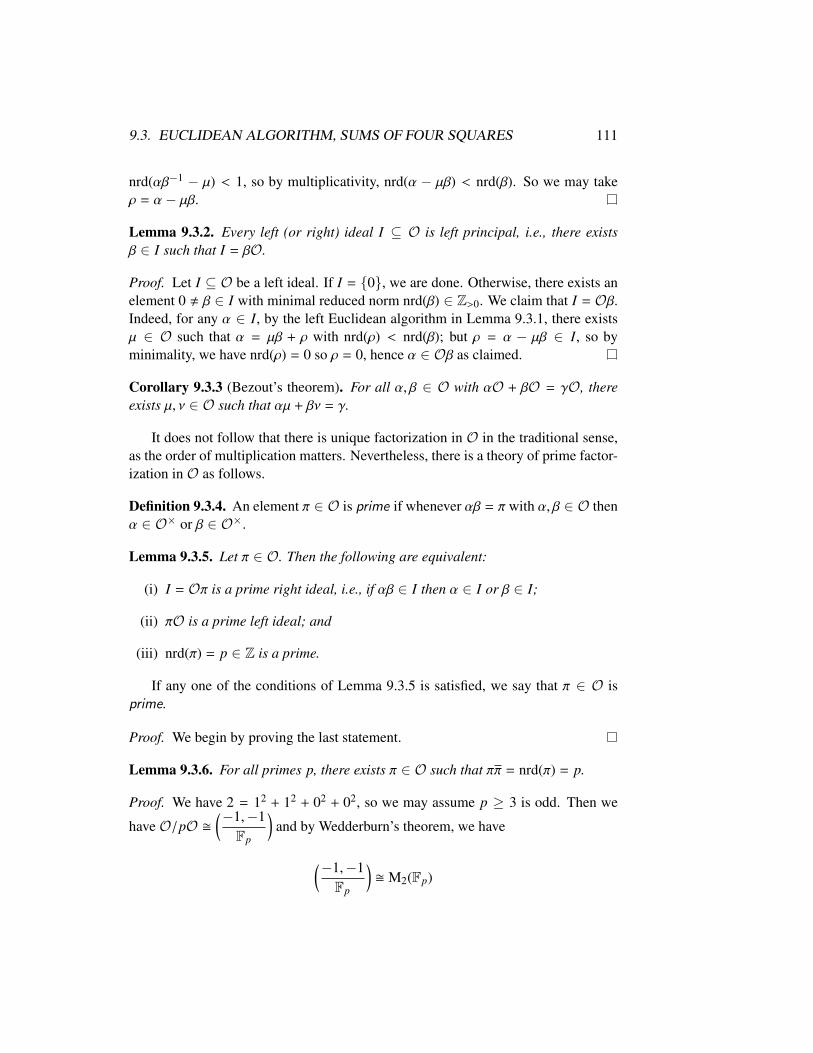
9.3. EUCLIDEAN ALGORITHM, SUMS OF FOUR SQUARES 111
nrd(αβ−1 − µ) < 1, so by multiplicativity, nrd(α − µβ) < nrd(β). So we may takeρ = α− µβ.
Lemma 9.3.2. Every left (or right) ideal I ⊆ O is left principal, i.e., there existsβ ∈ I such that I = βO.
Proof. Let I ⊆ O be a left ideal. If I = {0}, we are done. Otherwise, there exists anelement 0 , β ∈ I with minimal reduced norm nrd(β) ∈ Z>0. We claim that I = Oβ.Indeed, for any α ∈ I, by the left Euclidean algorithm in Lemma 9.3.1, there existsµ ∈ O such that α = µβ + ρ with nrd(ρ) < nrd(β); but ρ = α − µβ ∈ I, so byminimality, we have nrd(ρ) = 0 so ρ = 0, hence α ∈ Oβ as claimed.
Corollary 9.3.3 (Bezout’s theorem). For all α, β ∈ O with αO + βO = γO, thereexists µ, ν ∈ O such that αµ + βν = γ.
It does not follow that there is unique factorization in O in the traditional sense,as the order of multiplication matters. Nevertheless, there is a theory of prime factor-ization in O as follows.
Definition 9.3.4. An element π ∈ O is prime if whenever αβ = π with α, β ∈ O thenα ∈ O× or β ∈ O×.
Lemma 9.3.5. Let π ∈ O. Then the following are equivalent:
(i) I = Oπ is a prime right ideal, i.e., if αβ ∈ I then α ∈ I or β ∈ I;
(ii) πO is a prime left ideal; and
(iii) nrd(π) = p ∈ Z is a prime.
If any one of the conditions of Lemma 9.3.5 is satisfied, we say that π ∈ O isprime.
Proof. We begin by proving the last statement.
Lemma 9.3.6. For all primes p, there exists π ∈ O such that ππ = nrd(π) = p.
Proof. We have 2 = 12 + 12 + 02 + 02, so we may assume p ≥ 3 is odd. Then we
have O/pO �(−1,−1Fp
)and by Wedderburn’s theorem, we have
(−1,−1Fp
)� M2(Fp)

112 CHAPTER 9. THE HURWITZ ORDER
so there exists a left ideal I mod p ⊂ O/pO with dimFp(I mod p) = 2. Let
I = {α ∈ O : α mod p ∈ I mod p};
in particular we have pO ( I ( O. Then I ⊂ O is a left ideal, and I , O. ButI = βO is left principal by Lemma 9.3.2.
We claim that nrd(β) = p. Since p ∈ I, we have p = βµ for some µ ∈ O,whence nrd(p) = p2 = nrd(β) nrd(µ) so nrd(β) | p2. We cannot have nrd(β) = 1 ornrd(β) = p2, as these would imply I = O or I = pO, impossible. So nrd(β) = p.
Definition 9.3.7. An element α ∈ O is primitive if α < nO for all n ∈ Z.
[[Define left divisibility, etc.?]]
Theorem 9.3.8 (Conway–Smith). Let α ∈ O be primitive and let a = nrd(α). Factora = p1 p2 · · · pr into a product of primes. Then there exists π1, π2, . . . , πr ∈ O suchthat
α = π1π2 · · · πr, and nrd(πi) = pi for all i.
Moreover, any other such factorization is of the form
α = (π1γ1)(γ−11 π2γ
−12 ) · · · (γ−1
r−1πr) (9.3.9)
where γ1, . . . , γr ∈ O×.
The factorization (9.3.9) is said to be obtained from α = π1 · · · πr by unit migra-tion.
Theorem 9.3.10. Every integer n ≥ 0 is the sum of four squares, i.e., there existst, x, y, z ∈ Z such that n = t2 + x2 + y2 + z2.
Proof. We seek an element β ∈ Z〈i, j, k〉 such that nrd(β) = n. By multiplicativity,it is sufficient to treat the case where n = p is prime. We obtain π ∈ O such thatnrd(π) = p by Lemma 9.3.6. But now the result follows from Lemma 9.2.4, as thereexists γ ∈ O× such that πγ ∈ Z〈i, j, k〉.
9.4 Sums of three squares
9.5 Extensions and further reading
Exercises
9.1. Show that
O = Z + Zi + Z j + Z(1 + i + j + k
2
)

9.5. EXTENSIONS AND FURTHER READING 113
is an order in B =
(−1,−1Q
).
9.2. Check that the map
O/3O → M2(F3)
i, j 7→(0 −11 0
),
(1 11 −1
)from Lemma 9.2.1 is the isomorphism obtained from the representation on theleft ideal generated by ε = i + j + k.
9.3. Draw the subgroup lattice for SL2(F3), indicating normal subgroups (and theirquotients).
9.4. Let O ⊂ B =
(−1,−1Q
)be the Hurwitz order.
a) Consider the natural ring homomorphism O → O ⊗Z F2 = OF2 givingthe reduction of the algebra O modulo 2. Show that #OF2 = 16, thatO×F2
� A4 the alternating group on 4 elements. Conclude that OF2 �M2(F2) and hence that OF2 is not a quaternion algebra over F2.
b) Show that AutF2(OF2) � S 4 (automorphisms as an F2-algebra). Moregenerally, if F is a field of characteristic 2, show that OF = O ⊗Z F hasAutF OF is an extension of SL2(F) by the additive group F2.
This kind of construction, considered instead over the octonions, arises whenconstructing the exceptional group G2 in characteristic 2 [Wil09, §4.4.1].
9.5. Show that2T � 〈r, s, t | r2 = s3 = t3 = rst = −1〉
(cf. (9.5)).
9.6. Let Λ = Z4 + (( 12 ,
12 ,
12 ,
12 ) + Z4) be the image of the Hurwitz order O under
the natural embedding O ↪→ H � R4. Show that for every x ∈ R4, thereexists λΛ such that ‖λ‖2 ≤ 1/2. [Hint: without loss of generality we maytake 0 ≤ xi ≤ 1/2 for all i; then show we may take x1 + x2 + x3 + x4 ≤ 1;conclude that the maximum value of ‖x‖2 with these conditions occurs at thepoint ( 1
2 ,12 , 0, 0).]


Chapter 10
Quaternion algebras over localfields
In this chapter, we classify quaternion algebras over local fields; this generalizes theclassification of quaternion algebras over R.
10.1 Local quaternion algebras
Having spent the first part of this book exploring the properties of quaternion alge-bras, we now seek to classify them over a nice class of fields. Over any field F wehave the matrix ring M2(F), and if F is a finite field or an algebraically closed fieldF, then any quaternion algebra over F is isomorphic to the matrix ring. The ‘first’quaternion algebra, of course, was the division ring H of Hamiltonians, and this ringis the only division quaternion ring over R up to isomorphism.
In this section, we will classify quaternion algebras over a field F that is in somesense similar to R. We will insist that the field F is equipped with a topology com-patible with the field operations in which F is Hausdorff and locally compact (everyelement of F has a compact neighborhood). To avoid trivialities, we will insist thatthis topology is not the discrete topology (where every subset of F is open): such atopological field is called a local field.
For purposes of illustration, we consider local fields F that contain the rationalnumbers Q as a dense subfield. Such a field F is the completion of Q with respectto an absolute value | |, so is obtained as the set of equivalence classes of Cauchysequences, and has a topology induced by the metric d(x, y) = |x− y|. By a theoremof Ostrowski, such an absolute value is equivalent to either the usual archimedean
115

116 CHAPTER 10. QUATERNION ALGEBRAS OVER LOCAL FIELDS
absolute value or a p-adic absolute value, defined by |0|p = 0 and
|c|p = p− ordp(c) for c ∈ Q×,
where ordp(c) is the power of p occurring in c in its unique factorization (taken to benegative if p divides the denominator of c written in lowest terms).
Just as elements of R can be thought of infinite decimals, an element of Qp canbe thought of in its p-adic expansion
a = (. . . a3a2a1a0.a−1a−2 · · · a−k)p =
∞∑n=−k
an pn
where each ai ∈ {0, . . . , p−1} are the digits of a. We continue “to the left” because adecimal expansion is a series in the base 1/10 < 1 and instead we have a base p > 1.Inside Qp is the ring Zp of p-adic integers , the completion of Z with respect to | |p:the ring Zp consists of those elements of Qp with an = 0 for n < 0. The ring Zp
might be thought of intuitively as Z/p∞Z, if this made sense: they were first definedin this context by Hensel, who wanted a uniform language for when a Diophantineequation has a solution modulo pn for all n.
By construction, the ring Zp and the field Qp come equipped with a topologyarising from its metric dp(x, y) = |x− y|p. With respect to this topology, in fact Zp
is compact and Qp is locally compact. It is easiest to see this by viewing Zp as aprojective limit with respect to the natural maps Z/pn+1Z→ Z/pnZ:
Zp = lim←−nZ/pnZ
=
x = (xn)n ∈∞∏
n=0
Z/pnZ : xn+1 ≡ xn (mod pn) for all n ≥ 0
. (10.1.1)
In other words, each element of Zp is a compatible sequence of elements in Z/pnZfor each n. The equality (10.1.1) is just a reformulation of the notion of Cauchysequence for Z, and so for the purposes of this introduction it can equally well betaken as a definition. As for the topology in (10.1.1), each factor Z/pnZ is given thediscrete topology, the product
∏∞n=0 Z/pnZ is given the product topology, and Zp is
given the restriction topology. Since each Z/pnZ is compact (it is a finite set!), byTychonoff’s theorem the product
∏∞n=0 Z/pnZ is compact; and Zp is closed inside
this product (a convergent limit of Cauchy sequences is a Cauchy sequence), so Zp
is compact. The set Zp is a neighborhood of 0, indeed, it is the closed ball of radius1 around 0:
Zp = {x ∈ Qp : |a|p ≤ 1}.

10.2. LOCAL FIELDS 117
In a similar way, the disc of radius 1 around any a ∈ Qp is a compact neighborhoodof a homeomorphic to Zp, so Qp is locally compact.
As is evident from this argument, although Qp is Hausdorff and locally compact,it has a rather strange topology, akin to a Cantor set: Qp is totally disconnected (thelargest connected subsets consist of single points). Nevertheless, being able to maketopological arguments like the one above is the whole point of looking at local fieldslike Qp: our understanding of algebraic objects is informed by the topology.
In particular, we have a result for quaternion algebras over Qp that is quite anal-ogous to that over R.
Theorem 10.1.2. There is a unique division quaternion algebra B over Qp, up toisomorphism. In fact, if p , 2, then B is given by
B �(e, pQp
)where e ∈ Z is a quadratic nonresidue modulo p.
We approach this theorem in two ways in this section. The first way is using thelanguage of quadratic forms, and for that we use the classification of isomorphismclasses of quaternion algebras in terms of similarity classes of ternary quadraticforms. The following proposition then implies Theorem 10.1.2.
Proposition 10.1.3. There is a unique ternary anisotropic quadratic form Q overQp,up to similarity. If p , 2, then Q ∼ 〈1,−e,−p〉 where e is a quadratic nonresiduemodulo p.
This proposition can be proved using some rather direct manipulations with quad-ratic forms. On the other hand, it has the defect that quadratic forms behave differ-ently in characteristic 2, and so one may ask for a more uniform proof. This is thesecond way that we approach the proof of Theorem 10.1.2: we extend the absolutevalue onQp to one on a division quaternion algebra B, and use this extension to showthat B is unique by direct examination of its valuation ring and two-sided maximalideal. While it requires a bit more theory, this method of proof also can be used toclassify central division algebras over Qp in much the same manner.
10.2 Local fields
Definition 10.2.1. A topological ring is a ring A equipped with a topology suchthat the ring operations (addition, negation, and multiplication) are continuous. Ahomomorphism of topological rings is a ring homomorphism that is continuous. Atopological field is a field that is also a topological ring in such a way that divisionby a nonzero element is continuous.

118 CHAPTER 10. QUATERNION ALGEBRAS OVER LOCAL FIELDS
A very natural way to equip a ring with a topology that occurs throughout math-ematics is by way of an absolute value; to get started, we consider such notions firstfor fields. Throughout, let F be a field.
Definition 10.2.2. An absolute value on F is a map
| | : F → R≥0
such that:
(i) |x| = 0 if and only if x = 0;
(ii) |xy| = |x|y for all x, y ∈ F; and
(iii) |x + y| ≤ |x| + |y| for all x, y ∈ F (triangle inequality ).
An absolute value | | on F gives F the structure of a topological field by the metricd(x, y) = |x− y|. Two absolute values | |, ‖ ‖ on F are equivalent if there exists c > 0such that |x| = ‖x‖c for all x ∈ F; equivalent absolute values induces the sametopology on F.
Definition 10.2.3. An absolute value is nonarchimedean if |x + y| ≤ sup{|x|, |y|}for all x, y ∈ F (ultra metric inequality ), and archimedean otherwise.
Example 10.2.4. The fields R and C are topological fields with respect to the usualarchimedean absolute value.
Remark 10.2.5. A field is archimedean if and only if it satisfies the archimedeanproperty : for all x ∈ F×, there exists n ∈ Z such that |nx| > 1. In particular, a fieldF equipped with an archimedean absolute value has char F = 0.
Example 10.2.6. Every field has the trivial (nonarchimedean) absolute value, de-fined by |0| = 0 and |x| = 1 for all x ∈ F×; the trivial absolute value induces thediscrete topology on F.
A nonarchimedean absolute value on a field F arises naturally by way of a valu-ation, as follows.
Definition 10.2.7. A valuation of a field F is a map v : F → R ∪ {∞} such that:
(i) v(x) =∞ if and only if x = 0;
(ii) v(xy) = v(x) + v(y) for all x, y ∈ F; and
(iii) v(x + y) ≥ min(v(x), v(y)) for all x, y ∈ F.

10.2. LOCAL FIELDS 119
A valuation is discrete if the value group v(F×) is discrete inR (has no accumulationpoints).
Here, we set the convention that x +∞ = ∞ + x = ∞ for all x ∈ R ∪ {∞}.By (ii), the value group v(F×) is indeed a subgroup of the additive group R, and soalthough an absolute value is multiplicative, a valuation is additive.
Example 10.2.8. For p ∈ Z prime, the the map v(x) = ordp(x) is a valuation on Q.
Example 10.2.9. Let k be a field and F = k(t) the field of rational functions over k.For f (t) = g(t)/h(t) ∈ k(t) \ {0}, define v( f (t)) = deg g(t) − deg h(t) and v(0) = ∞.Then v is a discrete valuation on F.
Given the parallels between them, it should come as no surprise that a valuationgives rise to an absolute value on F by defining |x| = c−v(x) for any c > 1; the inducedtopology on F is independent of the choice of c. By condition (iii), the absolute valueassociated to a valuation is nonarchimedean.
Example 10.2.10. The trivial valuation is the valuation v satisfying v(0) = ∞ andv(x) = 0 for all x ∈ F×. The trivial valuation gives the trivial absolute value on F.
Two valuations v, w are equivalent if there exists a ∈ R>0 such that v(x) = aw(x)for all x ∈ F; equivalent valuations give the same topology on a field. A nontrivialdiscrete valuation is equivalent after rescaling (by the minimal positive element inthe value group) to one with value group Z, since a nontrivial discrete subgroup of Ris cyclic; we call such a discrete valuation normalized.
Given a field F with a nontrivial discrete valuation v, we have the valuation ringR = {x ∈ F : v(x) ≥ 0}. We have R× = {x ∈ F : v(x) = 0} since v(x) + v(x−1) =
v(1) = 0 for all x ∈ F×. The valuation ring is a local ring with unique maximal ideal
p = {x ∈ F : v(x) > 0} = R \ R×.
An element π ∈ p with smallest valuation is called a uniformizer, and comparingvaluations we see that πR = (π) = p. Since p ( R is maximal, the quotient k = R/pis a field, called the residue field of R (or of F).
Recall that a topological space is locally compact if each point has a compactneighborhood.
Definition 10.2.11. A local field is a Hausdorff, locally compact topological fieldwith a nondiscrete topology.
In a local field, we can hope to understand its structure by local considerations ina compact neighborhood, hence the name.
Local fields have a very simple classification as follows.
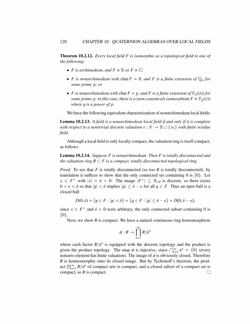
120 CHAPTER 10. QUATERNION ALGEBRAS OVER LOCAL FIELDS
Theorem 10.2.12. Every local field F is isomorphic as a topological field to one ofthe following:
• F is archimedean, and F � R or F � C;
• F is nonarchimedean with char F = 0, and F is a finite extension of Qp forsome prime p; or
• F is nonarchimedean with char F = p, and F is a finite extension of Fp((t)) forsome prime p; in this case, there is a (non-canonical) isomorphism F � Fq((t))where q is a power of p.
We have the following equivalent characterization of nonarchimedean local fields.
Lemma 10.2.13. A field is a nonarchimedean local field if and only if it is completewith respect to a nontrivial discrete valuation v : F → R ∪ {∞} with finite residuefield.
Although a local field is only locally compact, the valuation ring is itself compact,as follows.
Lemma 10.2.14. Suppose F is nonarchimedean. Then F is totally disconnected andthe valuation ring R ⊂ F is a compact, totally disconnected topological ring.
Proof. To see that F is totally disconnected (so too R is totally disconnected), bytranslation it suffices to show that the only connected set containing 0 is {0}. Letx ∈ F× with |x| = δ > 0. The image |F×| ⊆ R>0 is discrete, so there exists0 < ε < δ so that |y| < δ implies |y| ≤ δ − ε for all y ∈ F. Thus an open ball is aclosed ball
D(0, δ) = {y ∈ F : |y| < δ} = {y ∈ F : |y| ≤ δ− ε} = D[0, δ− ε];
since x ∈ F× and δ > 0 were arbitrary, the only connected subset containing 0 is{0}.
Next, we show R is compact. We have a natural continuous ring homomorphism
φ : R→∞∏
n=1
R/pn
where each factor R/pn is equipped with the discrete topology and the product isgiven the product topology. The map φ is injective, since
⋂∞n=1 p
n = {0} (everynonzero element has finite valuation). The image of φ is obviously closed. ThereforeR is homeomorphic onto its closed image. But by Tychonoff’s theorem, the prod-uct
∏∞n=1 R/pn of compact sets is compact, and a closed subset of a compact set is
compact, so R is compact.

10.3. UNIQUE DIVISION RING, FIRST PROOF 121
One key property of local fields we will use is Hensel’s lemma: it is the nonar-chimedean analogue of Newton’s method.
Lemma 10.2.15 (Hensel’s lemma). Let F be a nonarchimedean local field with val-uation v and valuation ring R, and let f (x1, . . . , xn) ∈ R[x1, . . . , xn] with n ≥ 1.Suppose that a = (ai)i ∈ Rn satisfies
k = v( f (a1, . . . , an)) > 2v( f ′(a1, . . . , an)) ≥ 0.
Then there exists a = (ai)i ∈ Rn such that f (a) = 0 and
ai ≡ ai (mod pk)
for all i = 1, . . . , n.
10.3 Unique division ring, first proof
We now seek to classify quaternion algebras over local fields. First, suppose F isarchimedean. When F = C, the only quaternion algebra over C up to isomorphismis B � M2(C). When F = R, by the theorem of Frobenius (Corollary 3.5.5), there isa unique quaternion division algebra over R. The classification of quaternion alge-bras over nonarchimedean local fields is quite analogous to the classification over R;indeed, we have the following.
Theorem 10.3.1. Let F , C be a local field. Then there is a unique division quater-nion algebra B over F up to F-algebra isomorphism.
To prove this theorem, from the first paragraph of this section we may assume Fis a nonarchimedean local field with discrete valuation v.
We approach the proof of Theorem 10.3.1 from two vantage points. In thissection, we give a proof using quadratic forms (which excludes the case wherechar F = 2); in the next section, we give another proof by extending the valuation(including all characteristics).
By Theorems 4.4.5 and 4.5.5, to prove Theorem 10.3.1 it is equivalent to provethe following proposition.
Proposition 10.3.2. Let F , C be a local field. Then there is a unique nonsingularanisotropic ternary quadratic form over F up to similarity.
So our task becomes a hands-on investigation of ternary quadratic forms over F.The theory of quadratic forms over F is linked to that over its residue field k, so wefirst need to examine isotropy of quadratic forms over a finite field.

122 CHAPTER 10. QUATERNION ALGEBRAS OVER LOCAL FIELDS
Lemma 10.3.3. A quadratic space V over a finite field with dimF V ≥ 3 is isotropic.
This statement is elementary (Exercise 10.1).
Lemma 10.3.4. Suppose char k , 2. Let Q : M → R be a nonsingular quadraticform over R. Then the reduction Q mod p : M⊗Rk→ k of Q modulo p is nonsingularover k; moreover, Q is isotropic over R if and only if Q mod p is isotropic.
Lemma 10.3.4 is a consequence of Hensel’s lemma (Lemma 10.2.15). Combin-ing these two lemmas, we obtain the following.
Proposition 10.3.5. Suppose char k , 2. Let Q : M → R be a nonsingular quadraticform over R with M of rank ≥ 3. Then Q is isotropic.
Considering valuations, we also deduce the following from Lemma 10.3.4.
Lemma 10.3.6. Suppose char k , 2. Then #F×/F×2 � (Z/2Z)2 and is representedby the classes of 1, e, π, eπ where e ∈ R× is any element which reduces modulo p toa nonsquare in k.
We first consider the case char k , 2.
Proof of Proposition 10.3.2 (char k , 2). Let Q � 〈a,−b,−c〉 be a nonsingular, an-isotropic ternary quadratic form over F. Rescaling the basis elements by a power ofthe uniformizer, we may assume that v(a), v(b), v(c) ∈ {0, 1}. Then, by the pigeon-hole principle on this set of valuations, we may rescale the form and permute thebasis to assume that a = 1 and 0 = v(b) ≤ v(c). If v(b) = v(c) = 0 then the quadraticform modulo p is nonsingular, so by Lemma 10.3.3 it is isotropic and by Lemma10.3.4 we conclude Q is isotropic, a contradiction.
We are left with the case v(b) = 0 and v(c) = 1. By Lemma 10.3.6, we mayassume b = 1 or b = e where e is a nonsquare in k. If b = 1, then the form isobviously isotropic, so we have b = e. Similarly, we have c = π or c = eπ. In fact,the latter case is similar to the former: scaling by e we have
〈1,−e,−eπ〉 ∼ 〈−1, e,−π〉
and since 〈−1, e〉 � 〈1,−e〉 (Exercise 10.2), we have Q ∼ 〈1,−e,−π〉.To conclude, we show that the form 〈1,−e,−π〉 is anisotropic. Suppose that
x2 − ey2 = πz2 with x, y, z ∈ F3 not all zero. By homogeneity, we may assumex, y, z ∈ R and at least one of x, y, z ∈ R×. Reducing modulo p we have x2 ≡ ey2
(mod p) so since e is a nonsquare we have v(x), v(y) ≥ 1. But this implies thatv(z) = 0 and so v(πz2) = 1 = v(x2 − ey2) ≥ 2, a contradiction.
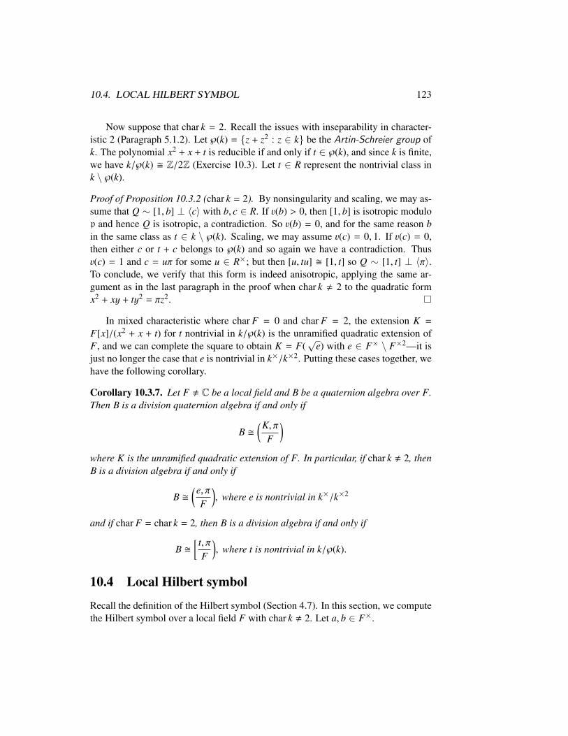
10.4. LOCAL HILBERT SYMBOL 123
Now suppose that char k = 2. Recall the issues with inseparability in character-istic 2 (Paragraph 5.1.2). Let ℘(k) = {z + z2 : z ∈ k} be the Artin-Schreier group ofk. The polynomial x2 + x + t is reducible if and only if t ∈ ℘(k), and since k is finite,we have k/℘(k) � Z/2Z (Exercise 10.3). Let t ∈ R represent the nontrivial class ink \ ℘(k).
Proof of Proposition 10.3.2 (char k = 2). By nonsingularity and scaling, we may as-sume that Q ∼ [1, b] ⊥ 〈c〉 with b, c ∈ R. If v(b) > 0, then [1, b] is isotropic modulop and hence Q is isotropic, a contradiction. So v(b) = 0, and for the same reason bin the same class as t ∈ k \ ℘(k). Scaling, we may assume v(c) = 0, 1. If v(c) = 0,then either c or t + c belongs to ℘(k) and so again we have a contradiction. Thusv(c) = 1 and c = uπ for some u ∈ R×; but then [u, tu] � [1, t] so Q ∼ [1, t] ⊥ 〈π〉.To conclude, we verify that this form is indeed anisotropic, applying the same ar-gument as in the last paragraph in the proof when char k , 2 to the quadratic formx2 + xy + ty2 = πz2.
In mixed characteristic where char F = 0 and char F = 2, the extension K =
F[x]/(x2 + x + t) for t nontrivial in k/℘(k) is the unramified quadratic extension ofF, and we can complete the square to obtain K = F(
√e) with e ∈ F× \ F×2—it is
just no longer the case that e is nontrivial in k×/k×2. Putting these cases together, wehave the following corollary.
Corollary 10.3.7. Let F , C be a local field and B be a quaternion algebra over F.Then B is a division quaternion algebra if and only if
B �(K, π
F
)where K is the unramified quadratic extension of F. In particular, if char k , 2, thenB is a division algebra if and only if
B �(e, π
F
), where e is nontrivial in k×/k×2
and if char F = char k = 2, then B is a division algebra if and only if
B �[ t, π
F
), where t is nontrivial in k/℘(k).
10.4 Local Hilbert symbol
Recall the definition of the Hilbert symbol (Section 4.7). In this section, we computethe Hilbert symbol over a local field F with char k , 2. Let a, b ∈ F×.

124 CHAPTER 10. QUATERNION ALGEBRAS OVER LOCAL FIELDS
We begin with the case where F is archimedean. If F = C, then the Hilbertsymbol is identically 1. If F = R, then
(a, b)R =
1, if a > 0 or b > 0;−1, if a < 0 and b < 0.
Lemma 10.4.1. The Hilbert symbol over a nonarchimedean local field F is bimulti-plicative, i.e.
(a, bc)F = (a, b)F(a, c)F and (ab, c)F = (a, c)F = (b, c)F
for all a, b, c ∈ F×.
Remark 10.4.2. The bimultiplicativity property of the local Hilbert symbol is a spe-cial property and does not extend to a general field!
Proof. This will follow from the direct computation below (10.4.3), but it is helpfulto know this fact independently.
We appeal to Theorem 4.5.5(vi): we have (a, b)F = 1 if and only if b ∈ NK/F(K×)where K = F[x]/(x2 − a). If K is not a field, then (a, b)F = 1 identically, so itis certainly multiplicative. Otherwise, F×/NK/F(K×) � Z/2Z: when char k , 2,this follows from Lemma 10.3.6, but it is true in general. Multiplicativity is thenimmediate.
Since the Hilbert symbol is well-defined up to squares, the symbol (a, b)F isdetermined by the values with a, b ∈ {1, e, π, eπ} where e is a nonsquare in k×. Lets = (−1)(#k−1)/2, so that s = 1,−1 according as −1 is a square in k. Then we have:
(a, b)F 1 e π eπ1 1 1 1 1e 1 1 −1 −1π 1 −1 s −seπ 1 −1 −s s
(10.4.3)
The computation of this table is Exercise 10.7.
10.4.4. The following criteria follow from 10.4.3:
(a) If v(ab) = 0, then (a, b)F = 1.
(b) If v(a) = 0 and v(b) = v(π), then
(a, b)F =
(aπ
)=
1 if a ∈ k×2;−1 if a ∈ k× \ k×2.
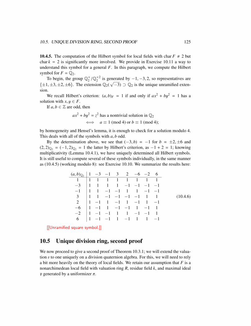
10.5. UNIQUE DIVISION RING, SECOND PROOF 125
10.4.5. The computation of the Hilbert symbol for local fields with char F , 2 butchar k = 2 is significantly more involved. We provide in Exercise 10.11 a way tounderstand this symbol for a general F. In this paragraph, we compute the Hilbertsymbol for F = Q2.
To begin, the group Q×2 /Q×22 is generated by −1,−3, 2, so representatives are
{±1,±3,±2,±6}. The extension Q2(√−3) ⊃ Q2 is the unique unramified exten-
sion.We recall Hilbert’s criterion: (a, b)F = 1 if and only if ax2 + by2 = 1 has a
solution with x, y ∈ F.If a, b ∈ Z are odd, then
ax2 + by2 = z2 has a nontrivial solution in Q2
⇐⇒ a ≡ 1 (mod 4) or b ≡ 1 (mod 4);
by homogeneity and Hensel’s lemma, it is enough to check for a solution modulo 4.This deals with all of the symbols with a, b odd.
By the determination above, we see that (−3, b) = −1 for b = ±2,±6 and(2, 2)Q2 = (−1, 2)Q2 = 1 the latter by Hilbert’s criterion, as −1 + 2 = 1; knowingmultiplicativity (Lemma 10.4.1), we have uniquely determined all Hilbert symbols.It is still useful to compute several of these symbols individually, in the same manneras (10.4.5) (working modulo 8): see Exercise 10.10. We summarize the results here:
(a, b)Q2 1 −3 −1 3 2 −6 −2 61 1 1 1 1 1 1 1 1−3 1 1 1 1 −1 −1 −1 −1−1 1 1 −1 −1 1 1 −1 −13 1 1 −1 −1 −1 −1 1 12 1 −1 1 −1 1 −1 1 −1−6 1 −1 1 −1 −1 1 −1 1−2 1 −1 −1 1 1 −1 −1 16 1 −1 −1 1 −1 1 1 −1
(10.4.6)
[[Unramified square symbol.]]
10.5 Unique division ring, second proof
We now proceed to give a second proof of Theorem 10.3.1; we will extend the valua-tion v to one uniquely on a division quaternion algebra. For this, we will need to relya bit more heavily on the theory of local fields. We retain our assumption that F is anonarchimedean local field with valuation ring R, residue field k, and maximal idealp generated by a uniformizer π.

126 CHAPTER 10. QUATERNION ALGEBRAS OVER LOCAL FIELDS
Let K ⊇ F be a finite extension of fields. Then there exists a unique valuation won K such that w|F = v, and we say that w extends v: this valuation is defined by
w(x) =v(NK/F(x))
[K : F]; (10.5.1)
in particular, K is also a nonarchimedean local field. (The only nontrivial thing tocheck is condition (iii), and this can be derived from the fact that
v(NK/F(x)) ≥ 0⇒ v(NK/F(x + 1)) ≥ 0
for x ∈ K and this follows by a direct examination of the minimal polynomial of x.)
Lemma 10.5.2. The integral closure of R in K is the valuation ring S = {x ∈ K :w(x) ≥ 0}, and S is an R-order in K.
A finite extension K/F is unramified if a uniformizer π for F is also a uniformizerfor K. There is a unique unramified extension of F of any degree f ∈ Z≥1 and sucha field corresponds to the unique extension of the residue field k of degree f . In anunramified extension K/F of degree [K : F] = f , we have NK/F(K×) = R×π fZ, sob ∈ NK/F(K×) if and only if f | v(b).
10.5.3. If char k , 2, then by Hensel’s lemma, the unramified extension of degree2 is given by adjoining a square root of the unique nontrivial class in k×/k×2; ifchar k = 2, then the unramified extension of degree 2 is given by adjoining a rootof the polynomial x2 + x + t where t is a nontrivial class in the Artin-Schreier groupk/℘(k).
Let K ⊇ F be a finite separable extension of fields. We say K/F with e = [K : F]is totally ramified if a uniformizer πK has the property that πe
K is a uniformizer forF. For any finite separable extension K/F of degree n, there is a (unique) maximalunramified subextension Kun/F, and the extension K/Kun is totally ramified.
K
Kun
e
F
f
We say that e = [K : Kun] is the ramification degree and f = [Kun : F] the inertialdegree, and we have the fundamental equality
n = [K : F] = e f . (10.5.4)

10.5. UNIQUE DIVISION RING, SECOND PROOF 127
We now seek to generalize these theorems to the noncommutative case. Let D bea central simple division algebra over F with dimF D = [D : F] = n2. We extend thevaluation v to a map
w : D→ R ∪ {∞}
α 7→v(ND/F(α))
[D : F]=v(nrd(α))
n,
where the equality follows from the fact that ND/F(α) = nrd(α)n (see Section 6.7).
Lemma 10.5.5. The map w defines a valuation on D, i.e., the following hold:
(i) w(α) =∞ if and only if α = 0.
(ii) w(αβ) = w(α) + w(β) = w(βα) for all α, β ∈ D.
(iii) w(α + β) ≥ min(w(α), w(β)) for all α, β ∈ D.
(iv) w(D×) is discrete in R.
Proof. Statement (i) is clear (note it already uses that D is a division ring). Statement(ii) follows from the multiplicativity of nrd and v. To prove (iii), we may assumeβ , 0 and so β ∈ D×. We have w(α+ β) = w(β) +w(αβ−1 + 1). But the restriction ofw to F(αβ−1) is a discrete valuation, so w(αβ−1 + 1) ≥ min(w(αβ−1), w(1)) so by (ii)w(α + β) ≥ min(w(α), w(β)), as desired. Finally, (iv) holds since w(D×) ⊆ v(F×)/nand the latter is discrete.
From Lemma 10.5.5, we say that w is a discrete valuation on D since it satisfiesthe same axioms as for a field. It follows from Lemma 10.5.5 that the set
O = {α ∈ D : w(α) ≥ 0}
is a ring, called the valuation ring of D.
Proposition 10.5.6. O is the unique maximal R-order in D, consisting of all elementsof D that are integral over R.
Proof. First, we prove that
O = {α ∈ D : α is integral over R}.
In one direction, suppose α ∈ D is integral over R. Since R is integrally closed, byLemma 8.3.10 the coefficients of the minimal polynomial f (x) ∈ F[x] of α belong toR. Since D is a division ring, f (x) is irreducible and hence the reduced characteristic
128 CHAPTER 10. QUATERNION ALGEBRAS OVER LOCAL FIELDS
polynomial g(x) is a power of f (x) and thus has coefficients in R. The reduced normis the constant coefficient of g(x), so α ∈ O.
Now suppose α ∈ O, so that w(α) ≥ 0, and let K = F(α). Let f (x) ∈ F[x] bethe minimal polynomial of α. We want to conclude that f (x) ∈ R[x] knowing thatw(α) ≥ 0. But the restriction of w to K is the unique extension of v to K, and sothis is a statement about the extension K/F of local fields and therefore follows fromthe theory in the commutative case. For completeness, we give the proof. Let L bea splitting field of f (x) containing K. Then v extends to a unique valuation wL on L.At the same time, the norm w on D restricts to a discrete valuation on K and henceby equivalence of valuations, we have wL(α) ≥ 0. But now if f (x) =
∏ni=1(x− αi) =
xn + · · ·+ a0 ∈ F[x] with αi ∈ L, then wL(αi) = a0 = w(α) ≥ 0. Thus the coefficientsof f (symmetric functions in the αi) belong to R, and so α is integral over R.
We can now prove that O is an R-order. Scaling any element α ∈ D× by anappropriate power of π gives it positive valuation, so OF = D. So to conclude wemust show that O is finitely generated as an R-module. For this purpose, we mayassume that D is central over F, since the center K = Z(D) is a field extension of Fof finite degree and the integral closure of R in K is finitely generated as an R-module(Lemma 10.5.2). A central division algebra is separable, so we may apply Lemma8.4.1: every α ∈ O is integral over R and O is a ring, so the lemma implies that O isan R-order.
Finally, it follows immediately that O is a maximal R-order: by Corollary 8.3.9,every element of an R-order is integral over R, andO contains all such elements.
Remark 10.5.7. For a quaternion division algebra D, we can argue more directly inthe proof of Proposition 10.5.6 using the reduced norm: see Exercise 10.14.
It follows from Proposition 10.5.6 that O is a finitely generated R-submodule ofD. But R is a PID (every ideal is a power of the maximal ideal p) so in fact O is freeof rank [D : F] over R. We have
O× = {α ∈ D : w(α) = 0} (10.5.8)
since w(α−1) = −w(α) and α ∈ O× if and only if nrd(α) ∈ R×. Consequently,
P = {α ∈ D : w(α) > 0} = O \ O×
is the unique maximal two-sided ideal of O. Therefore O is a noncommutative localring, a ring with a unique maximal left (or right) ideal.
We are now prepared to give the second proof of the main result in this chapter(Theorem 10.3.1). By way of analogy, we consider the commutative case: for anextension L of F of degree [L : F] = n, we have a ramification degree e and aninertial degree f with e f = n (10.5.4). The same will be true when B is a division

10.5. UNIQUE DIVISION RING, SECOND PROOF 129
quaternion algebra: we will show that O/P is a quadratic field extension of k andhence that B contains an unramified separable quadratic extension K of F (extendingthe analogy, that f = 2); and then computing with valuations we will conclude thatP2 = πO (and e = 2) from which the result follows.
Proof of Theorem 10.3.1. Suppose that v : F → Z≥0 ∪ {∞} is normalized and letj ∈ P have minimal (positive) valuation w( j) ≥ 1/2. Then for any 0 , α ∈ P wehave w(α j−1) = w(α) − w( j) ≥ 0 so α j−1 ∈ O so α ∈ O j. Thus P = O j = jO =
O jO, since P is a two-sided ideal. Arguing in the same way, since
w( j) ≤ w(π) = v(π2) = 1 ≤ w( j2),
we conclude that P ⊇ πO ⊇ P2 = j2O. The map α 7→ α j yields an isomorphismO/P ∼−→ P/P2 of k-vector spaces, so
4 = dimkO/πO ≤ dimkO/P + dimk P/P2 = 2 dimkO/P (10.5.9)
and thus dimkO/P ≥ 2; in particular, O/P , k.SinceO\P = {x ∈ O : w(x) = 0} = O×, the ringO/P is a division algebra over
k and hence a finite division ring. But then by Wedderburn’s theorem (Exercises 3.12and 5.11, or Exercise 6.16), the ring O/P is a field. Thus, there exists i ∈ O suchthat O/P = k(i), since k is a finite field. Then K = F(i) is an unramified separablequadratic extension of F and consequently dimkO/P = f = 2. Therefore equalityholds in (10.5.9), and so P2 = πO.
By Exercise 6.13, there exists b ∈ F× such that B �(K, b
F
). But B is a division
ring if and only if b ∈ F× \ NK/F(K×) by Theorems 4.5.5 and 5.3.8. Since K/F isunramified we have NK/F(K×) = R×π2Z, so we may take b = π (Exercise 5.3) and
B �(K, π
F
)is the unique division quaternion algebra over F.
Corollary 10.5.10. If F is nonarchimedean and B =
(K, bF
), then B � M2(F) if K is
unramified over F (so v is split or inert in K) and v(b) = 0.
Remark 10.5.11. Let B �(K, π
F
)be a division quaternion algebra over F, so that K
is a separable quadratic subfield and j2 = π. As above, in analogy with the case offield extensions, we define the ramification degree of B over F as e(B/F) = 2 andthe inertial degree of B over F as f (B/F) = 2 and note the equality e(B/F) f (B/F) =
4 = [B : F], as in the commutative case. This equality carries over more generally todivision algebras; see Exercise 10.17.

130 CHAPTER 10. QUATERNION ALGEBRAS OVER LOCAL FIELDS
10.6 Topology
In this section, we conclude with some discussion about the topology of algebrasover local fields.
Let F be a local field. Then F is locally compact (by definition) but is not itselfcompact. The subgroup F× = F \ {0} is equipped the subspace topology; it is openin F so F× is locally compact—this is quite visible when F = R,C is archimedean.If F is nonarchimedean, with valuation ring R and valuation v, then F× is totallydisconnected and further R× = {x ∈ R : v(x) = 0} ⊂ R is closed so is a topologicalabelian group that is compact (and totally disconnected).
Now let B be a finite-dimensional F-algebra. Then as a vector space over F, ithas a unique topology compatible with the topology on F, as any two norms on atopological vector F-space (extending the norm on F) are equivalent (the sup normis equivalent to the sum of squares norm, etc.). Two elements are close in the topol-ogy on B if and only if their coefficients are close with respect to a (fixed) basis: forexample, two matrices in Mn(F) are close if and only if all of their coordinate entriesare close. Consequently, B is locally compact topological ring (take a compact neigh-borhood in each coordinate). It is also true that B× is a locally compact topologicalgroup: the norm NB/F : B× → F× is a continuous map, so B× is open in B, and anopen subset of a Hausdorff, locally compact space is locally compact in the subspacetopology.
Example 10.6.1. If B = Mn(F), then B× = GLn(F) is locally compact: any closed,bounded neighborhood that avoids the locus of matrices with determinant 0 is acompact neighborhood. When F is archimedean, this is quite visual: any matrixof nonzero determinant is at some finite distance away from the determinant zerolocus! Note however that GLn(F) is not itself compact since F× = GL1(F) is notcompact.
Now suppose F is nonarchimedean with valuation v and valuation ring R. ThenR is the maximal compact subring of F. Indeed, x ∈ F lies in a compact subring ifand only if v(x) ≥ 0 if and only if x is integral over R. The only new implication hereis the statement that if v(x) < 0 then x does not lie in a compact subring, and that isbecause the sequence xn = xn does not have a convergent subsequence as |xn| → ∞.
Next, let O be an R-order in B. Then O � Rn is a free R-module of finite rank.Choosing a basis, the above argument shows that O is compact as the Cartesianpower of a compact set. The groupO× is therefore also compact because it is closed:for γ ∈ O, we have γ ∈ O× if and only if NB/F(γ) ∈ R× ⊂ R and R× = {x ∈ R :v(x) = 0} ⊆ R is closed.

10.7. SPLITTING FIELDS 131
Example 10.6.2. For R = Zp ⊆ F = Qp and B = Mn(Qp), the order O = Mn(Zp)is compact (neighborhoods can be taken coordinatewise) and the subgroup O× =
GLn(Zp) is compact: there is no way to run off to infinity, either in a single coordinateor via the determinant.
10.6.3. Suppose B = D is a division ring. Then the valuation ring O is the max-imal compact subring of B, for the same reason as in the commutative case. Inthis situation, the unit group O× is a pro-solvable group! We have a filtrationO ⊃ P ⊃ P2 ⊃ . . . giving rise to a filtration
O× ⊃ 1 + P ⊃ 1 + P2 ⊃ . . . .
As in the second proof of Theorem 10.3.1, the quotient O/P is a finite extension ofthe finite residue field k, so (O/P)× is a cyclic abelian group. The maximal two-sidedideal P is principal, generated by an element j of minimal valuation, and multipli-cation by jn gives an isomorphism O/P ∼−→ Pn/Pn+1 of k-vector spaces (or abeliangroups) for all n ≥ 1.
Furthermore, for each n ≥ 1, we have an isomorphism of groups
Pn/Pn+1 ∼−→ (1 + Pn)/(1 + Pn+1)
α 7→ 1 + α.(10.6.4)
Therefore, O× = lim←−n(O/Pn)× is an inverse limit of solvable groups.
10.6.5. We will also want to consider norm 1 groups; for this, we assume that B is asemisimple algebra. Let
B×1 = {α ∈ B : nrd(α) = 1}.
Then B×1 is a closed subgroup of B×, since the reduced norm is a continuous function.If B is a divison ring and F is nonarchimedean, then B has a valuation ring O, andB×1 = O×1 is compact. If B is a division ring and F is archimedean, then B � H andB×1 � H×1 � SU(2) is compact (it is identified with the 3-sphere in R4). Finally, ifB is not a division ring, then either B is the product of two algebras or B is a matrixring over a division ring, and correspondingly B is not compact by considering thesubgroup (π, 1/π) or a unipotent subgroup.
10.7 Splitting fields
Proposition 10.7.1. Let B be a division quaternion ring over F, and let L be a sepa-rable field extension of F of finite degree. Then L is a splitting field for B if and onlyif [L : F] is even.

132 CHAPTER 10. QUATERNION ALGEBRAS OVER LOCAL FIELDS
Proof. We have B �(K, π
F
)where K is the unramified quadratic extension of F. Let
e, f be the ramification index and inertial degree of L. Then [L : F] = n = e f , so n iseven if and only if e is even or f is even.
But f is even if and only if L contains an unramified quadratic subextension,necessarily isomorphic to K; but then K splits B so L splits B.
Otherwise, L is linearly disjoint from K so K ⊗F L = KL is the unramified
quadratic extension of L. Therefore B⊗F L �(KL, π
L
). Let RL be the valuation ring
of L and let πL be a uniformizer for L. Then NKL/L(KL×) = R×L π2ZL . If L/F has
ramification index e, then π = uπeL for some u ∈ R×L . Putting these together, we see
that B ⊗F L is a division ring if and only if π is a norm from KL if and only if e iseven.
Corollary 10.7.2. If K/F is a separable quadratic field extension, then K ↪→ B.
In other words, B contains every separable quadratic extension of F!
10.8 Extensions and further reading
10.8.1. The p-adic numbers were developed by Hensel. In the early 1920s, Hasseused them in the study of quadratic forms and algebras over number fields. At thetime, what is now called the “local–global principle” then was called the the p-adictransfer from the “small” to the “large”.
10.8.2. Theory of local fields: [Neu99, Corollary V.1.2]. serre.
10.8.3. Weil started this game in his basic number theory.
10.8.4. Theory of local division rings more generally and noncommutative localrings.
10.9 Algorithmic aspects
Computing the Hilbert symbol
Exercises
10.1. Let k be a finite field and let Q : V → k be a ternary quadratic form. Showthat q is isotropic. [Hint: Reduce to the case of finding a solution to y2 = f (x)where f is a polynomial of degree 2. Then only the case #k odd remains; show

10.9. ALGORITHMIC ASPECTS 133
that f takes on at least (q + 1)/2 values in k but there are at most (q − 1)/2nonsquares in k.]
Conclude again that there is no division quaternion ring over a finite field k.
10.2. Let k be a finite field with char k , 2 and let e ∈ k×. Show that there is anisometry 〈−1, e〉 � 〈1,−e〉.
10.3. Let k be a finite field with even cardinality. Show that #k/℘(k) = 2, where ℘(k)is the Artin-Schreier group.
10.4. Let F , C be a local field and let Q be a nonsingular ternary quadratic formover F. Show that Q is isotropic over any quadratic field extension of F.
10.5. Let B be a division quaternion algebra over a nonarchimedean local field F.Give another proof that the unramified quadratic extension K of F embeds inB as follows.
Suppose it does not: then for all x ∈ O, the extension F(x)/F is ramified, sothere exists a ∈ R such that x − a ∈ P ∩ K(x); then write x = x0 = a + jx1,where P = jO, and iterate to conclude that x =
∑∞n=0 an jn with an ∈ R. But
F( j) is complete so O ⊆ F( j), a contradiction.
10.6. Let B be a division quaternion algebra over the nonarchimedean local field F.
a) Show that B is a complete, locally compact topological ring and that Ois the maximal compact subring of B.
b) Show that O× and B×/F× are compact topological groups.
c) Conclude that the smooth, irreducible complex representations of B× arefinite dimensional, and compare this with the alternative B � M2(F).
10.7. Show that the table of Hilbert symbols (10.4.3) is correct.
10.8. Let F be a local field and K the unramified quadratic extension of F. Computethe K-left regular representation of a division quaternion algebra B over F(2.2.8) and identify the maximal order R and the maximal ideal P.
10.9. Prove a descent for the Hilbert symbol, as follows. Let K be a finite extensionof the local field F with char F , 2 and let a, b ∈ F×. Show that (a, b)K =
(a,NK/F(b))F .
10.10. Show that the table of Hilbert symbols (10.4.6) is correct by considering theequation ax2 + by2 ≡ 1 (mod 8).

134 CHAPTER 10. QUATERNION ALGEBRAS OVER LOCAL FIELDS
10.11. [[Alternative method for computing the Hilbert symbol.]]
10.12. One can package Paragraph 10.4.4 together with multiplying by squares toprove the following more general criterion. For a, b ∈ F×, we have
(a, b)F = (−1)v(a)v(b)(q−1)/2(
aπ
)v(b)bπ
v(a)
where a = a0πv(a) and b = b0π
v(b) (and v(π) = 1).
10.13. Consider B =
(−1,−1Q2
)and letO = Z2⊕Z2i⊕Z2 j⊕Z2(1+i+ j+i j)/2. Show
that B is a division ring. Give an explicit formula for the discrete valuation won B (extending the valuation v on Q2) and prove that O is its valuation ring.
10.14. Let B be a division quaternion algebra over F. Show that α ∈ B is integralover R if and only if nrd(x), nrd(x + 1) ∈ R if and only if w(x), w(x + 1) ≥ 0,where w is the valuation on B.
10.15. Let B be a division quaternion algebra over a nonarchimedean local field F,and let O be the valuation ring. Show that every one-sided (left or right) idealof O is a power of the maximal ideal J and hence is two-sided.
10.16. Let F be a nonarchimedean local field, let B = M2(F) and O = M2(R). Showthat there are q + 1 right O-ideals of norm p corresponding to the elements ofP1(k) or to the lines in k2.
10.17. Let D be a finite-dimensional division algebra over a nonarchimedean localfield F of degree [D : F] = n2 with valuation ring O and two-sided ideal P.Show that O/P is finite extension of k of degree n and Jn = OπO.
10.18. Show that (10.6.4) is an isomorphism of (abelian) groups.

Chapter 11
Quaternion algebras over globalfields
In this chapter, we discuss quaternion algebras over global fields and characterizethem up to isomorphism.
11.1 Ramification
To motivate the classification of quaternion algebras over Q, we consider by analogya classification of quadratic fields. For this purpose, we restrict to the following class.
Definition 11.1.1. A quadratic field F = Q(√
d) of discriminant d ∈ Z is mildlyramified if 8 - d.
A quadratic field F is mildly ramified if and only if F = Q(√
m) where m , 1 isodd and squarefree; then d = m or d = 4m according as m = 1, 3 (mod 4).
Let F = Q(√
d) be a mildly ramified quadratic field of discriminant d ∈ Z andlet R be its ring of integers. The primes p that ramify in F, so pR = p2 for a primeideal p ⊂ R, are precisely those with p | d.
But a discriminant d can be either positive or negative; to put this bit of data onthe same footing, we define the set of places of Q to be the primes together withthe symbol ∞, and we make the convention that ∞ ramifies in F if d < 0 and isunramified if d > 0. This convention is sensible, because when d < 0 we haveonly one way to embed Q(
√d) ↪→ C up to complex conjugation—only one place
above∞ in F, so ramified—whereas there are two essentially distinct ways to embedQ(√
d) ↪→ R when d > 0 (two places above∞ in F).Let F = Q(
√d) be a mildly ramified quadratic field, and let Ram(F) be the set
of places that ramify in F. The set Ram(F) determines F up to isomorphism, since
135

136 CHAPTER 11. QUATERNION ALGEBRAS OVER GLOBAL FIELDS
the discriminant of F is the product of the odd primes in Ram(F), multiplied by 4 if2 ∈ Ram(F) and by−1 if∞ ∈ Ram(F). (For bookkeeping reasons, in this context itwould probably therefore be better to consider 4 and −1 as primes, but we will resistthe inducement here.) However, not every finite set of places Σ occurs: the product dcorresponding to Σ is a discriminant if and only if d ≡ 0, 1 (mod 4). We call this aparity condition on the set of ramifying places of a mildly ramified quadratic field:
2 ∈ Σ ⇐⇒ there are an odd number of primes p ∈ Σ with p ≡ −1 (mod 4)
(with the convention that∞ is congruent to −1 (mod 4)).Note that if Σ is a finite subset of places of Q and 2 < Σ, then precisely one of
either Σ or Σ ∪ {∞} satisfies the parity condition; accordingly, if we define m(Σ) tobe the product of all odd primes in Σ multiplied by−1 if∞ ∈ Σ, then we can recoverΣ from m(Σ).
We have proven the following result.
Lemma 11.1.2. The maps F 7→ Ram(F) and Σ 7→ m(Σ) furnishes a bijection{ Mildly ramified quadratic fieldsQ(√
d) up to isomorphism
}←→
{ Finite subsets of places of Qsatisfying the parity condition
}←→ {Squarefree odd integers m , 1} .
This classification procedure using sets of ramifying primes and discriminantsworks as well for quaternion algebras over Q. Let B be a quaternion algebra overQ. When is a prime p ramified in B? In Chapter 10, we saw that the completionBp = B⊗Q Qp is either a division ring or the matrix ring M2(Qp). Further, when Bp
is a division ring, the valuation ring Op ⊂ Bp is the unique maximal order, and theunique maximal ideal Pp ⊂ Op satisfies pOp = P2
p. So by analogy with the quadraticcase, we say that a place v is ramified in B if the completion Bv is a division ring, andotherwise v is unramified (or split).
There are only finitely many places where B =
(a, bQ
)is ramified: by the calcula-
tion of the Hilbert symbol (Paragraph 10.4.4), if p - 2ab is prime, then (a, b)Qp = 1and p is split in B. Therefore # Ram(B) <∞.
Let Ram(B) be the set of ramified places of B. Not every finite subset Σ ofplaces can occur as Ram(B) for a quaternion algebra B. It turns out that the paritycondition here is that we must have #Σ even. So again, if Σ is a finite set of primes,then precisely one of either Σ or Σ ∪ {∞} can occur as Ram(B). We define thediscriminant of B to be the product disc(B) of primes that ramify in B, so disc(B) asquarefree positive integer.
The main result of this chapter, specialized to the case F = Q, is then the follow-ing.

11.2. HILBERT RECIPROCITY OVER THE RATIONALS 137
Theorem 11.1.3. The maps B 7→ Ram(B) and Σ 7→∏p∈Σ p furnish bijections{ Quaternion algebras over Q
up to isomorphism
}←→
{ Finite subsets of places of Qof even cardinality
}←→ {d ∈ Z>0 squarefree} .
The composition of these maps is B 7→∏p∈Ram(B) p = disc(B).
Having stated Theorem 11.1.3, we will spend the next two sections giving a self-contained proof, assuming two statements from basic number theory (quadratic reci-procity, and primes in arithmetic progression). Although the proofs presented do notgeneralize to an arbitrary global field, the argument is simple enough and its structureis good motivation for the more involved treatment in the chapter ahead.
11.2 Hilbert reciprocity over the rationals
To begin, we look into the parity condition: it has a simple reformulation in terms ofthe Hilbert symbol (Section 4.7). For a place v of Q, let Qv denote the completionof Q at the absolute value associated to v: if v = p is prime, then Qv = Qp is thefield of p-adic numbers; if v = ∞ is the real place, then Qv = R. For a, b ∈ Q×, weabbreviate (a, b)Qv = (a, b)v.
Proposition 11.2.1 (Hilbert reciprocity). For all a, b ∈ Q×, we have∏v
(a, b)v = 1, (11.2.2)
the product taken over all places v of Q.
The product (11.2.2) is well-defined, because we just saw that for all primesp - 2ab, we have (a, b)p = 1. The following corollary is then immediate.
Corollary 11.2.3. Let B be a quaternion algebra over Q. Then the set Ram(B) isfinite of even cardinality.
The law of Hilbert reciprocity, as it turns out, is a core premise in number theory:it is equivalent to the law of quadratic reciprocity(
pq
) (qp
)= (−1)
p−12
q−12 (11.2.4)
for odd primes p, q together with the supplement(−1p
)= (−1)
p−12 and
(2p
)= (−1)
p2−18 (11.2.5)

138 CHAPTER 11. QUATERNION ALGEBRAS OVER GLOBAL FIELDS
for odd primes p.We now give a proof of Hilbert reciprocity (Proposition 11.2.1), assuming the
law of quadratic reciprocity and its supplement.
Proof of Proposition 11.2.1. Since the Hilbert symbol is bilinear, it suffices to provethe statement when a, b ∈ Z are equal to either −1 or a prime number. The Hilbertsymbol is also symmetric, so we may interchange a, b.
If a = b = −1, then B =
(a, bQ
)=
(−1,−1Q
)is the rational Hamiltonians, and
we have (−1,−1)∞ = (−1,−1)2 = −1 and (−1,−1)v = 1 if v , 2,∞, by thecomputation of the even Hilbert symbol (Paragraph 10.4.5). Similarly, the cases witha = −1, 2 follow from the supplement (11.2.5), and are requested in Exercise 11.1.
So we may suppose a = p and b = q are primes. If p = q then( p, pQ
)�
(−1, pQ
)and we reduce to the previous case, so we may suppose p , q. Since p, q > 0, wehave (p, q)∞ = 1. We have (p, q)` = 1 for all primes ` - 2pq. We have
(p, q)p = (q, p)p =
(qp
)and (p, q)q =
(pq
)by Paragraph 10.4.4. Finally, we have
(p, q)2 = −1 if and only if p, q ≡ 3 (mod 4)
i.e., (p, q)2 = (−1)(p−1)(q−1)/4, again by the computation of the even Hilbert symbol(10.4.5). Thus the product becomes∏
v
(p, q)v = (−1)(p−1)(q−1)/4(
pq
) (qp
)= 1
by quadratic reciprocity.
Hilbert reciprocity has several aesthetic advantages over the law of quadraticreciprocity. For one, it is simpler to write down! Also, Hilbert believed that hisreciprocity law is a kind of analogue of Cauchy’s integral theorem, expressing anintegral as a sum of residues (11.9.6). The fact that a normalized product over allplaces is trivial also arises quite naturally: if we define for x ∈ Q× and a prime p thenormalized absolute value
|x|p = p− ordp(x),
and |x|∞ the usual archimedean absolute value, then∏v
|x|v = 1

11.2. HILBERT RECIPROCITY OVER THE RATIONALS 139
by unique factorization in Z; this is called the product formula for Q, for obviousreasons.
From the tight relationship between quaternion algebras and ternary quadraticforms, we obtain the following corollary.
Corollary 11.2.6. Let Q be a nonsingular ternary quadratic form over Q. Then theset of places v such that Qv is anisotropic is finite and of even cardinality.
In particular, by Corollary 11.2.6 we have that if Qv is isotropic for all but oneplace v of Q, then Qv is in fact isotropic for all places v.
Proof. In the bijection of Theorem 4.4.5, the quadratic form Q corresponds to a
quaternion algebra B =
(a, bQ
), and by Theorem 4.5.5, Q is isotropic if and only if
B is split if and only if (a, b)Q = 1. By functoriality, the same is true over eachcompletion Qv for v a place of Q, and therefore the set of places v where Qv isisotropic is precisely the set of ramified places in B. The result then follows byHilbert reciprocity.
To conclude this section, we show that every allowable product of Hilbert sym-bols is obtained.
Proposition 11.2.7. Let Σ be a finite set of places of Q of even cardinality. Thenthere exists a quaternion algebra B over Q with Ram(B) = Σ.
Just as with Hilbert reciprocity, Proposition 11.2.7 touches on a deep statementin number theory concerning primes.
Theorem 11.2.8 (Primes in arithmetic progression). Given a, n ∈ Z coprime, thereare infinitely many primes p ≡ a (mod n).
We now prove Proposition 11.2.7 assuming Theorem 11.2.8.
Proof. Let d =∏
p∈Σ p be the product of the primes in Σ, and let u = −1 if∞ ∈ Σ
and u = 1 otherwise. Let d∗ = ud. We consider quaternion algebras of the form
B =
(d∗, q∗
Q
)with q∗ = uq (and q prime) satisfying certain congruence conditions to ensureRam(B) = Σ. To this end, we seek a prime q such that
q∗ is a quadratic nonresidue modulo p for all odd p | d (11.2.9)

140 CHAPTER 11. QUATERNION ALGEBRAS OVER GLOBAL FIELDS
and
q∗ ≡1 (mod 8), if 2 - d;
5 (mod 8), if 2 | d.(11.2.10)
There exists a prime satisfying the conditions (11.2.9)–(11.2.10) by the theoremon primes in arithmetic progression (Theorem 11.2.8), since the condition to be aquadratic nonresidue is a congruence condition on q∗ and hence on q modulo p.
We now verify that B has Ram(B) = Σ. We have (d∗, q∗)∞ = u by choice of signsand (d∗, q∗)p = 1 for all p - 2dq. We compute that
(d∗, q∗)p =
(q∗
p
)= −1 for all odd p | d
by (11.2.9). For p = 2, we find that (d∗, q∗)2 = −1 or (d∗, q∗)2 = 1 according as 2 | dor not by the computation of the even Hilbert symbol (10.4.5). This shows that
Σ ⊆ Ram(B) ⊆ Σ ∪ {q}.
The final symbol (d∗, q∗)q is determined by Hilbert reciprocity (Proposition 11.2.1):since #Σ is already even, we must have (d∗, q∗)q = 1 and Σ = Ram(B).
11.3 Hasse–Minkowski theorem over the rationals
To complete the proof of Theorem 11.1.3, we need to show that the association B 7→Ram(B) is injective (on isomorphism classes).
Proposition 11.3.1. Let A, B be quaternion algebras overQ. Then A � B if and onlyif Ram(A) = Ram(B) if and only if Av � Bv for all (but one) places v.
The statement of Proposition 11.3.1 is a local–global principle: the global iso-morphism class is determined by the local behavior at primes. For example, we havethe following consequence.
Corollary 11.3.2. Let B be a quaternion algebra over Q. Then B � M2(Q) if andonly if Bp � M2(Qp) for all primes p.
By the equivalence between quaternion algebras and quadratic forms (Chapter 4and specifically Section 4.4), the statement of Proposition 11.3.1 is equivalent to thestatement that a ternary quadratic form overQ is isotropic if and only if it is isotropicover all (but one) completions. In fact, the more general statement is true—and againwe come in contact with a deep result in number theory.

11.3. HASSE–MINKOWSKI THEOREM OVER THE RATIONALS 141
Theorem 11.3.3 (Hasse–Minkowski). Let Q be a quadratic form over Q. Then Q isisotropic if and only if Qv is isotropic for all places v of Q.
This theorem of Hasse–Minkowski is more generally called the Hasse principle(see Paragraph 11.9.4).
We will prove the Hasse–Minkowski theorem by induction on the number of vari-ables. Of particular interest is the case of (nondegenerate) ternary quadratic forms,for which we have the following theorem of Legendre.
Theorem 11.3.4 (Legendre). Let a, b, c ∈ Z be nonzero, squarefree integers that arerelatively prime in pairs. Then the quadratic form
ax2 + by2 + cz2 = 0
has a nontrivial solution if and only if a, b, c do not all have the same sign and
−ab, −bc, −ac are quadratic residues modulo |c|, |a|, |b|, respectively.
Proof. First, the conditions for solvability are indeed necessary. The condition onsigns is necessary for a solution in R. If ax2 + by2 + cz2 = 0 with x, y, z ∈ Q not allzero, then scaling we may assume x, y, z ∈ Z satisfy gcd(x, y, z) = 1; if p | c thenp - y (else p | x so p | z, contradiction), so (x/y)2 ≡ (−b/a) (mod |c|) so −ba is aquadratic residue modulo |c|; the other conditions hold by symmetry.
So suppose the conditions hold. Multiplying through and rescaling by squares,we may assume a, b are squarefree (but not necessarily coprime) and c = −1, and weseek a nontrivial solution to ax2 +by2 = z2. If a ∈ Q×2, then we are done. Otherwise,we need to solve
z2 − ax2
y2 = b = NQ(√
a)/Q
(z + x
√a
y
)for x, y, z ∈ Q and y , 0, i.e., we need to show that b is a norm from F = Q(
√a).
By hypothesis, a, b are not both negative and
b is a square modulo |a| and a is a square modulo |b|. (11.3.5)
We may also assume |a| ≤ |b|.We use complete induction on m = |a| + |b|. If m = 2, then we have the equation
±x2±y2 = z2 with the case both negative signs excluded, each of which has solutions.Now suppose that m > 2 so |b| ≥ 2, and let p | b be prime divisor. By hypothesis,there exist integers t, b′ such that t2 = a + bb′; taking a small residue, we may assume|t| < |b|/2. Thus
bb′ = t2 − a = NF/Q(t +√
a)

142 CHAPTER 11. QUATERNION ALGEBRAS OVER GLOBAL FIELDS
so bb′ is a norm from F. Thus b is a norm if and only if b′ is a norm. But
∣∣∣b′∣∣∣ =
∣∣∣∣∣∣ t2 − ab
∣∣∣∣∣∣ ≤ |b|4 + 1 < |b|
because |b| ≥ 2. Now write b′ = b′′u2 with b′′, u ∈ Z and b′′ squarefree. Then |b′′| ≤|b′| < |b| and b′′ is a norm if and only if b′ is a norm. With these manipulations, wepropagate the hypothesis that |a| is a square modulo |b′′| and |b′′| is a square modulo|a|. Therefore, the induction hypothesis applies to the equation ax2 + b′′y2 = z2, andwe are done.
Corollary 11.3.6. Let Q be a nondegenerate ternary quadratic form over Q. ThenQ is isotropic if and only if Qv is isotropic for all (but one) places v of Q.
Proof. If Q is isotropic, then Qv is isotropic for all v. For the converse, suppose thatQv is isotropic for all places v of Q. As in the proof of Legendre’s Theorem 11.3.4,we may assume Q(x, y, z) = ax2 + by2 − z2. The fact that Q is isotropic over Rimplies that a, b are not both negative. Now let p | a be odd. The condition that Qp
is isotropic is equivalent to (a, b)p = (b/p) = 1; putting these together, we concludethat b is a quadratic residue modulo |a|. The same holds for a, b interchanged, so(11.3.5) holds and the result follows.
We are now in a position to complete the proof of the Hasse–Minkowski theorem.
Proof of Theorem 11.3.3. We may assume that Q is nondegenerate in n ≥ 1 vari-ables. If n = 1, the statement is vacuous. If n = 2, the after scaling we may assumeQ(x, y) = x2 − ay2 with a ∈ Q×; since Qp is isotropic for all primes p, we havea ∈ Q×2
p so in particular ordp(a) is even for all primes p; since Q is isotropic at∞,we have a > 0; thus by unique factorization, we have a ∈ Q×2 and the result follows.If n = 3, the statement is proven in Corollary 11.3.6.
Now suppose n ≥ 4. Write Q = 〈a, b〉 ⊥ −Q′ where Q′ = 〈c1, . . . , cn−2〉 anda, b, ci ∈ Z. Let d = 2ab(c1 · · · cn−2) , 0. For each prime p | d, since Q is isotropic,there exists tp ∈ Q×p represented by both 〈a, b〉 and Q′ in Qp. (This requires asmall argument, which is left as Exercise 11.4.) Similarly, there exists t∞ ∈ R×represented by these forms in R.
By another application of primes in arithmetic progression (Exercise 11.5), thereexists t ∈ Q× such that:
(i) t ∈ tpQ×2p for all primes p | d,
(ii) t and t∞ have the same sign, and
(iii) p - t for all primes p - d except possibly for one prime q - d.

11.4. GLOBAL FIELDS 143
Now the quadratic form 〈a, b,−t〉 is isotropic for all p | d and at∞ by constructionand at all primes p - d except p = q since p - abt. Therefore, by case n = 3 (usingthe “all but one” in Corollary 11.3.6), the form 〈a, b,−t〉 is isotropic.
On the other side, if n = 4, then the form 〈t〉 ⊥ Q′ is isotropic by the sameargument. If n ≥ 5, then we apply the induction hypothesis to Q′: the hypothesisholds, since we have Q′ is isotropic at ∞ and all p | d by construction, and forall p - d the completion Q′p is a nondegenerate form in ≥ 3 variables over Zp sois isotropic by the results of Section 10.3, using Hensel’s lemma to lift a solutionmodulo the odd prime p.
Finally, putting these two together, we find that Q is isotropic over Q.
We conclude with the following consequence, which immediately implies Propo-sition 11.3.1.
Corollary 11.3.7. Let Q,Q′ be quadratic forms over Q in the same number of vari-ables. Then Q � Q′ are isometric if and only if Qv � Q′v for all places v.
Proof. The implication (⇒) is immediate. We prove (⇐) by induction on the num-ber of variables, the case of n = 0 variables being clear. By splitting the radical(Paragraph 4.2.12), we may assume that Q,Q′ are nondegenerate. Let a ∈ Q× berepresented by Q. Since Qv � Q′v the quadratic form 〈a〉 ⊥ Q′ is isotropic at v for allv, so Q′ represents a (Lemma 4.5.4). So in both cases, we can write Q � 〈a〉 ⊥ Q1and Q′ � 〈a〉 ⊥ Q′1 for quadratic forms Q1,Q′1 in one fewer number of variables. Fi-nally, by Witt cancellation (Proposition 4.2.16), from Qv � Q′v we have (Q1)v � (Q′1)vfor all v, so by induction, we have Q1 � Q′1, and thus Q � Q′.
In summary, the classification of quaternion algebras overQ embodies some deepstatements in number theory: quadratic reciprocity (and its reformulation in Hilbertreciprocity), the Hasse-Minkowski theorem (the local–global principle for quadraticforms), and the proofs use the theorem of primes in arithmetic progression! It is asmall blessing that we can make these essentially elementary arguments over Q. Inthe more general case, we must dig more deeply.
11.4 Global fields
In this chapter and in many that remain, we focus on a certain class of fields of arith-metic interest: a global field is a finite extension of Q (a number field) or Fp(t) (afunction field) for a prime p. Global fields are strongly governed by their comple-tions with respect to nontrivial absolute values, which are local fields. Throughoutthis text, we will return to this theme that global behavior is governed by local be-havior.

144 CHAPTER 11. QUATERNION ALGEBRAS OVER GLOBAL FIELDS
For the rest of this chapter, let F be a global field. The set of places of F is theset of equivalence classes of embeddings ιv : F → Fv where Fv is a local field andιv(F) is dense in Fv; two embeddings ιv : F → Fv and ι′v : F → F′v are equivalent ifthere is an isomorphism of topological fields φ : Fv → F′v such that ι′v = φ ◦ ιv.
Every valuation v : F → R ∪ {∞}, up to scaling, defines a place ιv : F →Fv where v is the completion of F with respect to the absolute value induced byv; we call such a place nonarchimedean, and using this identification we will writev for both the place of F and the corresponding valuation. For a nonarchimedeanplace v corresponding to a local field Fv, we denote by Rv its valuation ring, pv itsmaximal ideal, and kv its residue field. If F is a function field, then all places of Fare nonarchimedean. If F is a number field, a place F ↪→ R is called a real placeand a place F ↪→ C (equivalent to its complex conjugate) is called a complex place.A real or complex place is archimedean.
A global field F has a set of preferred embeddings ιv : F ↪→ Fv correspondingto each place v (equivalently, a preferred choice of absolute values | |v for each placev) such that the product formula holds: for all x ∈ F×, we have∏
v
|x|v = 1. (11.4.1)
The preferred absolute values are defined as follows.
11.4.2. The set of places of Q consists of the archimedean real place, induced by theembeddingQ ↪→ R and the usual absolute value |x|∞, and the set of nonarchimedeanplaces indexed by the primes p given by the embeddingsQ ↪→ Qp, with the preferredabsolute value
|x|p = p− ordp(x).
The statement of the product formula for x ∈ Q is∏p
p− ordp(x)|x|∞ = 1
and this follows from unique factorization in Z.
11.4.3. The set of places of Fp(t) is indexed by monic irreducible polynomials f (t) ∈Fp[t] with preferred absolute value
|x(t)| f = p−(deg f ) ord f (x)
and 1/t, the place at infinity, with preferred absolute value
|x(t)|1/T = pdeg x.

11.4. GLOBAL FIELDS 145
Then the statement of the product formula for x(t) ∈ Fp(t) is∏f
p(deg f ) ord f (x) = pdeg x
which follows from unique factorization in Fp[t].
11.4.4. More generally, let K/F be a finite extension of global fields. Let v be a placeof F with a preferred absolute value and let w is a place of K above v. Then thepreferred absolute value for w is
|x|w = |NK/F(x)|1/[K:F]v
for x ∈ K; note that if x ∈ F then
|x|w = |NK/F(x)|1/[K:F]v = |x|v,
so the absolute value | |w extends | |v, and thus this definition is compatible with fur-ther field extensions. [[In a potentially different way than valuations extend.]]
If F satisfies the product formula (11.4.1) with respect to preferred absolute val-ues, then so does K, since
∏w
|x|w =∏v
∏w|v|x|w
=∏v
|NK/F(x)|v = 1.
Therefore every global field satisfies the product formula with respect to preferredabsolute values.
11.4.5. Let F be a global field. Let S be a nonempty finite set of places of F con-taining all archimedean places of F (if F is a number field).
The ring of S-integers in F is the set
RS = {x ∈ F : v(x) ≥ 0 for all v < S}.
This definition makes sense as if v < S then by hypothesis v is nonarchimedean. Wewill often abbreviate R = RS .
Example 11.4.6. If F is a number field and S consists only of the archimedean placesin F then RS is the ring of integers in F, the integral closure of Z in F. If F is afunction field, corresponding to a curve X, then RS is the ring of all rational functionswith no poles outside S .

146 CHAPTER 11. QUATERNION ALGEBRAS OVER GLOBAL FIELDS
11.5 Ramification and discriminant
Let R = RS be an S-integer ring of F. Let B be a quaternion algebra over F.
Definition 11.5.1. Let v be a place of F. We say that B is ramified at v if Bv = B⊗F Fv
is a division ring; otherwise we say that B is split (or unramified) at v. Let Ram(B)denote the set of ramified places of B.
We use the term ramified for the following reason: if Bp is a division ring withvaluation ring Op, then pOp = P2 for a two-sided maximal ideal P, by the results ofSection 10.5. In a similar way, we will see that if p is a prime of R unramified in B,then there exist R-lattices of reduced norm p, so the term split is justified.
Lemma 11.5.2. The set Ram(B) of ramified places of B is finite.
Proof. Let B =
(K, bF
). Since F has only finitely many archimedean places, we may
suppose v is nonarchimedean. The extension K/F is ramified at only finitely manyplaces, so we may assume that K/F is unramified at v (the corresponding prime pis split or inert). Finally, we have v(b) = 0 for all but finitely many v, so we may
assume v(b) = 0. But then under these hypotheses, we have Bv =
(Kv, bFv
)is split, by
Corollary 10.5.10.
Motivated by the fact that the discriminant of a quadratic field extension is divis-ible by ramifying primes, we make the following definition.
Definition 11.5.3. The discriminant of B (relative to S) is the R-ideal
discS (B) =∏
p ramifiedp<S
p ⊆ R
obtained as the product of all primes p of R ramified in B.
11.5.4. When F is a number field and S consists of archimedean places only, so Ris the ring of integers of F, then we sometimes abbreviate discS (B) = disc(B). Notethat the discriminant discS (B) discards information about primes in S , so one shouldrefer to the set of ramified places for something independent of S .
The discriminant captures maximal R-orders in B, as follows: in particular, wewill see that maximal R-orders are characterized by their discriminants (and henceby the ramified places of B not in S).
Proposition 11.5.5. Let O be an R-order in B. Then O is maximal if and only ifdiscrd(O) = discS (B).

11.6. QUATERNION ALGEBRAS OVER GLOBAL FIELDS 147
Proof. The order O is maximal if and only if Op is maximal for all primes p of Rby Lemma 12.4.2, so it suffices to prove this statement locally. If B is split at p thenBp � M2(Fp), and an order is maximal if and only if it is isomorphic to M2(Rp). ButM2(Rp) has discriminant Rp by Exercise 13.3, and by Lemma 13.2.16, an order ismaximal if and only if it has discriminant Rp.
In a similar way, if B is ramified at p then Bp has a unique maximal order ofdiscriminant pRp, and the same argument applies.
Remark 11.5.6. The preceding results have an analogue in the case of a quadraticfield extension. Let K be a quadratic extension of F and suppose that 1/2 ∈ R. LetS be the integral closure of R in K. Then an R-order in K is maximal if and only ifits discriminant is equal to
disc(S ) =∏
p ramified in Kp<S
p ⊆ R.
11.5.7. It follows from Proposition 11.5.5 that
discS (B) | discrd(O).
So we define the level of an order O is the R-ideal
N = N(O) = discrd(O) discS (B)−1 ⊆ R.
11.6 Quaternion algebras over global fields
In the final section of this chapter, we deduce results characterizing isomorphismclasses of quaternion algebras assuming two results from number theory. In laterchapters, we give two self-contained proofs: an analytic approach using L-functions(Chapter [[??]]) and a cohomological approach using ideles (Chapter [[??]]). Thesearguments are more involved, and so for now we merely provide an exposition of thestatements.
The main result is as follows.
Theorem 11.6.1. The map B 7→ Ram(B) gives a bijection{ Quaternion algebras over Fup to isomorphism
}←→
{ Finite subsets of noncomplex placesof F of even cardinality
}.
Theorem 11.6.1 is comparable in depth and difficulty to the main theorems ofclass field theory; no proof that avoids these techniques is known. Several corollariesare important to note.

148 CHAPTER 11. QUATERNION ALGEBRAS OVER GLOBAL FIELDS
Corollary 11.6.2. Let B be a quaternion algebra over a global field. Then the set ofplaces of F where B is ramified is finite and of even cardinality.
Recall the definition of the Hilbert symbol (Section 4.7). For a place v of F, weabbreviate (a, b)Fv = (a, b)v; this symbol was computed for v an odd nonarchimedeanplace (10.4.3).
Corollary 11.6.3 (Hilbert reciprocity). Let F be a global field with char F , 2 andlet a, b ∈ F×. Then ∏
v
(a, b)v = 1.
The statement of Hilbert reciprocity (Corollary 11.6.2) can be rightly seen as alaw of quadratic reciprocity for number fields; indeed, it is equivalent to the law ofquadratic reciprocity over Q, as we saw in Section 11.2.
Corollary 11.6.4. Let A, B be quaternion algebras over F. Then A � B if and onlyif Ram(A) = Ram(B) if and only if Av � Bv for all (but one) places v of F.
In particular, B � M2(F) if and only if Ram(B) = ∅.
The statement of Corollary 11.6.4 is a local–global principle: the global isomor-phism class is determined by the local behavior at primes.
Corollary 11.6.5. A finite extension K/F splits B if and only if Kw/Fv splits Bv forall places w (over v) of K.
Proof. K splits B if and only if B⊗F K � M2(K) if and only if B⊗F Kw = Bv⊗Fv Kw �
M2(Kw) for all places w over v of K.
To prove Theorem 11.6.1, we will use the following two fact, whose proof wedelay until Chapter [[??]]: it is the case of what is known as the Hasse norm theoremfor quadratic extensions.
Claim 11.6.6. Let K/F be a separable quadratic F-algebra, and let b ∈ F×. Thenb ∈ NK/F(K×) if and only if b ∈ NKv/Fv(K
×w ) for all places v of F.
This statement is summarized as everywhere local norms are global norms. Since
every quaternion algebra is of the form B =
(K, bF
)with K separable over F, and
B � M2(F) if and only if b ∈ NK/F(K×), the claim is equivalent to the statement thatB � M2(F) if and only if Ram(B) = ∅.
11.7. HASSE–MINKOWSKI THEOREM 149
11.7 Hasse–Minkowski theorem
Claim 11.7.1. Let K/F be a separable quadratic F-algebra. Then K � F × F if andonly if Kv � Fv × Fv for all places v of F.
If char F , 2, and we can complete the square to obtain K = F(√
a) with a ∈F×, then this claim becomes a ∈ F×2 if and only if a ∈ F×2
v for all places v of F:everywhere local squares are global squares. This claim is the simpler, commutativeanalogue of the final statement in Corollary 11.6.4.
We now use these two claims to prove the Hasse–Minkowski theorem.
Theorem 11.7.2 (Hasse-Minkowski). Let F be a field with char F , 2 and let Q bea quadratic form over F. Then Q is isotropic if and only if Qv is isotropic over Fv forall places v of F.
Proof. It suffices to prove sufficiency. We may assume, without loss of generality,that Q is nondegenerate. If n = dim Q = 1, the theorem is vacuous. If n = 2,then after scaling we may assume Q = 〈1,−a〉; the equivalence follows immediatelyfrom Claim 11.7.1. If n = 3, then we may take Q = 〈1,−a,−b〉, and the equivalencefollows from Claim 11.6.6.
11.8 Representative quaternion algebras
Write down explicit representation of quaternion algebras and maximal orders basedon their discriminant.
Over Q, can do this with formulas.More generally, use primes in arithmetic progression. See also [Lem11, Proposi-
tion 2.10, Proposition 6.9].
11.9 Extensions and further reading
11.9.1. Conway would tell us to take −1 as a prime.
11.9.2. Proof of quadratic reciprocity.
11.9.3. Primes in arithmetic progression.
11.9.4. Called the Hasse principle because of Hasse’s contribution over numberfields. See Fenster and SchwŁrmer [FS07]. [FS07].
11.9.5. The definitions for the preferred absolute values may seem boring, but wewill see later that they are natural from the perspective of Haar measure.

150 CHAPTER 11. QUATERNION ALGEBRAS OVER GLOBAL FIELDS
11.9.6. Hilbert saw his reciprocity law for the product of the Hilbert symbols as ananalogue of Cauchy’s integral theorem; more precisely (according to Shafarevich), itis the analogue of the corollary to Cauchy’s integral theorem that say that the sum ofthe residues of a holomorphic differential at all points of a Riemann surfaces is zero.In this analogy, the symbol (a, b)p is the analogue of the differential a db at the pointp.
11.10 Algorithmic aspects
Effective solution of conics, geometry of numbers.Computing the set of ramified places.Computing a representative algebra.
Exercises
11.1. Complete the proof of Hilbert reciprocity (Proposition 11.2.1) in the remainingcases (a, b) = (−1, 2), (2, 2), (−1, p), (2, p). In particular, show that(−1, 2
Q
)�
(2, 2Q
)� M2(Q)
and
(a, p)2 = (a, p)p =
(ap
)for a = −1, 2 (cf. Paragraph para:Hilbm1m1).
11.2. Show that the law of Hilbert reciprocity (Proposition 11.2.1) implies the law ofquadratic reciprocity; with the argument given in section 11.1, this completesthe equivalence of these two laws.
11.3. Show that Legendre’s theorem can be deduced from the statement where a, b >0 and c = −1.
11.4. Let Q = Q′ ⊥ Q′′ be an orthogonal sum of two nondegenerate quadratic formsover a field F. Show that Q is isotropic if and only if there exists c ∈ F that isrepresented by both Q′ and Q′′.
11.5. Let S be a finite set of places of Q containing∞. For each v ∈ S , let tv ∈ Q×vbe given. Show that there exists t ∈ Q× such that t ∈ tvQ×2
v for all v ∈ S andordp(t) = 0 for all p < S \ {∞} except (possibly) for one prime p = q.

11.10. ALGORITHMIC ASPECTS 151
By another application of primes in arithmetic progression (Exercise 11.5),there exists t ∈ Q× such that t ∈ tpQ×2
p for all primes p | d, t and t∞ have thesame sign, and p - t for all primes p - d except for one prime q - d.
11.6. Let F = Q(√
d) be a real quadratic field. Find a, b ∈ F× such that(a, b
F
)is a
division ring unramified at all finite places.
11.7. Let K ⊇ F be finite separable extension of global fields. Let B be a quaternionalgebra over K. We say that B descends to F if there exists a quaternionalgebra A over F such that A⊗F K � B. Show that B descends to F if and onlyif Ram(B) is invariant under Gal(K/F).
11.8. Show without using primes in arithmetic progression that over Q all possible(even cardinality) ramification sets can occur. Do this by using the Brauerrelation and linkage.


Chapter 12
Lattices and localization
Properties of a domain are governed in an important way by its localizations, andconsequently the structure of lattices, orders, and algebras can often be understood bylooking at their localizations and completions. This chapter develops these themes,a local-global principle that we will carry throughout the text.
12.1 Localization of integral lattices
A lattice over the integers Z is a
12.2 Localizations
Throughout this chapter, let R be a noetherian domain with field of fractions F.For a prime ideal p ⊆ R, we denote by
R(p) = {r/s : s < p} ⊆ F
the localization of R at p. (We reserve the simpler subscript notation for the comple-tion, which will feature more prominently.) Since R is a domain, the map R ↪→ R(p)is an embedding and we can recover R by
R =⋂p
R(p) =⋂m
R(m) ⊆ F (12.2.1)
where the intersections are over all prime ideals of R and all maximal ideals of R,respectively.
We now prove a version of the equality (12.2.1) for R-lattices.Let V be a finite-dimensional F-vector space and let M be an R-lattice in V . For
a prime p of R, let M(p) = M ⊗R R(p) = R(p)M. Then M(p) is an R(p)-lattice in V . Inthis way, M determines a collection (M(p))p indexed over the primes p of R.
153

154 CHAPTER 12. LATTICES AND LOCALIZATION
Lemma 12.2.2. Let M be an R-lattice in V. Then
M =⋂p
M(p) =⋂m
M(m) ⊆ V
where the intersection is over all prime (maximal) ideals p.
Proof. It suffices to prove the statement for maximal ideals since M(m) ⊆ M(p) when-ever m ⊃ p.
The inclusion M ⊆ ⋂m M(m) is clear. So let x ∈ V satisfy x ∈ ⋂
m M(m). Let
(M : x) = {r ∈ R : rx ∈ M}.
Then (M : x) is an ideal of R. For any maximal ideal m of R, since x ∈ M(m) thereexists 0 , rm ∈ R \ m such that rmx ∈ M. Thus rm ∈ (M : x) and so (M : x) is notcontained in any maximal ideal of R. Therefore (M : x) = R and hence x ∈ M.
Corollary 12.2.3. Let M,N be R-lattices in V. Then M ⊆ N if and only if M(p) ⊆ N(p)for all prime ideals p of R if and only if M(m) ⊆ N(m) for all maximal ideals m of R.
Proof. We have M =⋂p M(p) ⊆
⋂p N(p) = N and similarly form; the other inclusion
is clear.
Lemma 12.2.4. Let B be a finite-dimensional F-algebra. An R-lattice I ⊆ B is anR-order if and only if I(p) is an R(p)-order for all primes p of R if and only if Im is anRm-order for all maximal ideals m of R.
Proof. If I is an R-order then I(p) is an R(p)-order for all primes p, hence for allmaximal ideals m.
Conversely, suppose that Im is an Rm-order for all maximal ideals m. Then 1 ∈⋂m I(m) = I and for any α, β ∈ M we have αβ ∈ ⋂
m I(m) = I, so I is a subring of Band hence an order. The statement for prime ideals follows a fortiori.
A property like that of being an R-order is called a local property, and a lemmalike Lemma 12.2.4 is thereby called a local-global principle.
We now pass to completions. Let Rp denote the completion of R at p, and letFp = F ⊗R Rp be the completion of F at p and Vp = V ⊗F Fp.
Lemma 12.2.5. The map
M(p) 7→ Mp = M(p) ⊗R(p) Rp
yields a bijection between R(p)-lattices in V(p) and Rp-lattices in Vp, with inverse
Mp 7→ Mp ∩ V(p).
Proof. This lemma follows as above once we show that if M(p) is an R(p)-lattice, thenMp ∩ V(p) = M(p): for the details, see Exercise 12.2.

12.3. BITS OF COMMUTATIVE ALGEBRA AND DEDEKIND DOMAINS 155
12.3 Bits of commutative algebra and Dedekind domains
So far, we have worked with finitely generated modules. We pause to consider somerelevant bits of commutative algebra in our context.
12.3.1. A free R-module is projective; the converse is true when R is a local ringor PID. In particular, a finitely generated R-module is projective if and only if it islocally free (since R is noetherian). The ability to argue locally and then with freeobjects is very useful in our investigations (as well as many others), and so very oftenwe will restrict our attention to projective R-modules.
As a basic counterexample to keep in mind, let k be a field and R = k[x, y]. Thenthe R-module (x, y) is not projective (Exercise 12.1). Similarly, if R = Z/n2Z forn ∈ Z>1, then Z/nZ is not projective as an R-module.
There is a class of rings where finitely generated modules are projective, namelywhen R is a Dedekind domain: a (noetherian) integrally closed domain such thatevery nonzero prime ideal is maximal.
Example 12.3.2. Trivially, any field is a Dedekind domain.The rings Z and Fp[t] are Dedekind domains. If K is a finite extension of Q or
Fp(t), then the integral closure of Z or Fp[t] in K is a Dedekind domain.The localization or completion of a Dedekind domain R at a prime p is again a
Dedekind domain.
Suppose R is a Dedekind domain. Then every nonzero ideal a of R can be writtenuniquely as the product of prime ideals (up to reordering). A fractional ideal of R isa nonzero projective R-submodule a ⊆ F; a subset a ⊆ F is a fractional ideal if andonly if there exists d ∈ R \ {0} such that da ⊆ R is an ideal in the usual sense. Ifa, b are fractional R-ideals, then a ⊆ b if and only if a ⊗R R(p) = a(p) ⊆ b(p) for allprimes p, and hence equality holds if and only if it holds locally. Indeed, we havefor any fractional ideal a that a =
⋂p a(p). For every fractional ideal a of R, the set
a−1 = {a ∈ F : aa ⊆ R} is a fractional ideal with aa−1 = R. Therefore the set offractional ideals of R forms a group under multiplication.
The localization of a Dedekind domain is a discrete valuation ring (DVR), hencea PID. Consequently, every fractional ideal of R is locally principal, i.e., if a ⊆ R is afractional ideal, then for all primes p of R we have a(p) = a⊗R R(p) = apR(p) for someap ∈ R(p).
Let M ⊆ V be an R-lattice. Then M is a projective R-module, and it followsthe structure theorem of projective modules over Dedekind domains that M is com-pletely decomposable, i.e. there exist fractional ideals a1, . . . , an of R and elementsx1, . . . , xn ∈ V such that
M = a1x1 ⊕ · · · ⊕ anxn. (12.3.3)

156 CHAPTER 12. LATTICES AND LOCALIZATION
We call the elements x1, . . . , xn a pseudobasis for M with respect to the coefficientideals a1, . . . , an.
12.4 Lattices and localization
We now characterize in a simple way the conditions under which a collection (M(p))pof R(p)-lattices arise from a global R-lattice, as in the first section. We will see thatjust as a nonzero ideal of R can be factored uniquely into a product of prime ideals,and hence by the data of these primes and their exponents, so too can a lattice beunderstood by a finite number of localized lattices, once a “reference” lattice hasbeen chosen (to specify the local behavior of the lattice at the other places).
We retain the hypothesis that R is a Dedekind domain.
Proposition 12.4.1. Let M ⊆ V be an R-lattice. Then the map N 7→ (N(p))p estab-lishes a bijection between R-lattices N and collections (N(p))p where M(p) = N(p) forall but finitely many primes p.
This proposition gives an extension of the local-global principle for lattices: notonly can a lattice be recovered by its localizations, but any lattice is obtained from afixed one by making (arbitrary) choices at finitely many localizations.
Proof. Let N ⊆ V be an R-lattice. Then there exists 0 , r ∈ R such that rM ⊆ N ⊆r−1M. But r is contained in only finitely many prime (maximal) ideals of R, so forall but finitely many primes p we have that r is a unit in R(p) and thus M(p) = N(p).
So consider the set of collections (N(p))p where N(p) is an R(p)-lattice for eachprime p with the property that M(p) = N(p) for all but finitely many primes p of R.Given such a collection, we define N =
⋂(p) N(p) ⊆ V . Then N is an R-submodule
of F. We show it is an R-lattice in V . For each p such that M(p) , N(p), there existsrp ∈ R such that rpM(p) ⊆ N(p) ⊆ r−1
p M(p). Therefore, if r =∏p rp is the product of
these elements, then rM(p) ⊆ N ⊆ r−1M(p) for all primes p with M(p) , N(p). On theother hand, if M(p) = N(p) then already rM(p) ⊆ M(p) = N(p) ⊆ r−1N(p) = r−1M(p).Therefore by Corollary 12.2.3, we have rM ⊆ N ⊆ r−1M, and so N is an R-lattice.
By Lemma 12.2.2, the association (N(p))p 7→⋂p N(p) is an inverse to N 7→
(N(p))p. Conversely, given a collection (N(p))p, for a nonzero prime p, we have(⋂q Nq
)(p) = N(p) since (Rq)(p) = F so (Nq)(p) = V whenever q , p.
In this way, we can show that the property of being a maximal order is a localproperty.
Lemma 12.4.2. Let B be a finite-dimensional F-algebra. An R-order O ⊆ B ismaximal if and only if O(p) is a maximal R(p)-order for all primes p of R.

12.5. ADELIC COMPLETIONS 157
Proof. If O(p) is maximal for each prime p then by Corollary 12.2.3 we see that O ismaximal. Conversely, supposeO is maximal and suppose thatO(p) ( O′(p) is a propercontainment of orders for some nonzero prime p. Then the setO′ = (⋂
q,pOq)∩O′(p)
is an R-order properly containing O by Lemma 12.2.4 and Proposition 12.4.1.
12.5 Adelic completions
For a lattice M, all localizations M(p) are submodules of the vector space M(0) = Vover F, so for example, the notion of intersection makes sense. It is often helpful tobe able to do this with the completions as well; this gives us a preview for the addles,which will feature prominently later on.
Define the restricted direct product. The module embeds diagonally and is dense.Prove at least one nice thing.
12.6 Extensions and further reading
12.6.1. Noetherianness is only used when...
12.7 Exercises
12.1. Let k be a field and R = k[x, y]. Show that the R-module (x, y) is not projective.
12.2. Let V be a finite-dimensional vector space over F and I ⊆ V an R-lattice. Let pbe a prime of R, let R(p) be the localization of R at p and let Rp be the completionof R at p. Show that if I(p) ⊆ V(p) is an Rp-lattice then Ip∩V(p) = I(p). Concludethat Lemma 12.2.5 holds.
12.3. Prove Lemma 13.2.15: if R is a Dedekind domain and J ⊆ I ⊆ V are R-latticesin a finite-dimensional vector space V over F, then [I : J] is the product of theinvariant factors (or elementary divisors) of the torsion R-module I/J.
12.4. Find R-lattices I, J ⊆ V such that [I : J] = R but I , J (cf. Proposition13.2.14).
12.5. Consider the following ‘counterexamples’ to Proposition 12.4.1 for more gen-eral integral domains as follows. Let R = Q[x, y] be the polynomial ring intwo variables over Q, so that F = Q(x, y). Let V = F and I = R.
a) Show that yR has the property that yR , R for infinitely many primeideals p of R.
158 CHAPTER 12. LATTICES AND LOCALIZATION
b) Consider the collection of lattices given by Jp = f (x)Rp if p = (y, f (x))where f (x) ∈ Q[x] is irreducible and Jp = Rp otherwise. Show that⋂p Jp = (0).
Instead, to conclude that a collection (Jp)p of Rp-lattices arises from a globalR-lattice J, one needs that the collection forms a sheaf [[cite]].

Chapter 13
Discriminants
13.1 Discriminantal notions
Let x1, . . . , xn ∈ Rn, and let A be the matrix with columns xi. Then the volume ofthe box with edges vi (originating at the origin) has ordinary volume |det(A)|. Inthis way, we can measure the volume of a number field F by taking the volume of afundamental parallelepiped for its ring of integers R: if x1, . . . , xn is a Z-basis for Rand ι : F ↪→ F⊗QR � Rn, then the volume of R in this embedding is |det(A)| whereA is the matrix with columns ι(xi).
We could compute this volume in a different way: we have
|det(A)| =√|det(AtA)| =
√det(M)
where M has i jth entry equal to the ordinary dot product vi ·v j. The square volume hassome advantages: for example, the square volume of the ring of integers computedabove is the discriminant of R, an integer: indeed, the associated dot product is thetrace form (x, y) 7→ TrF/Q(xy) (with values in Z on R).
More generally, whenever we have a symmetric bilinear form T : F × F → F(associated to a quadratic form), we have a square volume given by the determinantdet(T (xi, x j))i, j: this is the (twice-)discriminant of the quadratic form Q associated toT (when char F , 2).
Now if B is a finite-dimensional algebra over F, we have a bilinear form (α, β) 7→TrB/F(αβ), and so in this manner we obtain a discriminant (“square volume”) mea-suring in some way the complexity of B.
In this section, we establish basic facts about discriminants, including how theybehave under inclusion (measuring index) and localization. For quaternion orders, itturns out that the discriminant so defined is always a square, and there is an intrinsicway to define the square root of this discriminant, called the reduced discriminant.
159

160 CHAPTER 13. DISCRIMINANTS
13.2 Discriminant
As in the commutative case, ramification and maximality of orders is intrinsicallyrelated to discriminants. In this section, we defined the discriminant and show that itbehaves well with respect to localization.
Let R be a noetherian domain and let F = Frac(R). Let B be a semisimple algebraover F with dimF B = n. For elements α1, . . . , αn ∈ B, we define
d(α1, . . . , αn) = det(trd(αiα j))i, j=1,...,n.
Let O ⊆ B be an R-order.
Definition 13.2.1. The discriminant of O is the ideal disc(O) of R generated by theset
{d(α1, . . . , αn) : α1, . . . , αn ∈ O}.
Although Definition 13.2.1 may look unwieldly, it works as well in the commu-tative case as in the noncommutative case. We can at least see immediately that ifO ⊆ O′ are R-orders, then disc(O′) | disc(O). And the function d itself transformsin a nice way as the systems αi vary (such as in under a change of basis), as follows.
Lemma 13.2.2. Let α1, . . . , αn ∈ B and suppose β1, . . . , βn ∈ B have the form βi =∑nj=1 mi jα j with mi j ∈ F. Let M = (mi j)i, j=1,...,n. Then
d(β1, . . . , βn) = det(M)2d(α1, . . . , αn). (13.2.3)
Proof. By properties of determinants, if αi = α j for some i , j, then d(α1, . . . , αn) =
0. Consequently, if α1, . . . , αn are linearly dependent (over F), then d(α1, . . . , αn) =
0. So we may assume that α1, . . . , αn are linearly independent and that β1, . . . , βn arelinearly independent as well, so the matrix M, a change of basis matrix, is invertible.But by Gaussian reduction, any invertible matrix is the product of elementary matri-ces, so it is enough to check that the equality holds when M is an elementary matrix.But in each of these cases (a diagonal matrix, a permutation matrix, or a transvectionmatrix), the equality is immediate.
Corollary 13.2.4. If α1, . . . , αn is an R-basis for O, then
disc(O) = d(α1, . . . , αn)R.
Example 13.2.5. Suppose char F , 2. Let B =
(a, bF
)with a, b ∈ R. Let O =
R⊕ Ri⊕ R j⊕ Ri j.

13.2. DISCRIMINANT 161
Then disc(O) is the principal R-ideal generated by
disc(1, i, j, i j) = det
2 0 0 00 2a 0 00 0 2b 00 0 0 −2ab
= −(4ab)2.
The calculation when char F = 2 is Exercise 13.1.
13.2.6. More generally, if O is completely decomposable with
O = a1α1 ⊕ · · · ⊕ anαn
such as in (12.3.3), then from (13.2.3) we have
disc(O) = (a1 · · · an)2 disc(α1, . . . , αn).
Example 13.2.7. Let B = Mn(F) and O = Mn(R). Then disc(O) = R (Exercise13.3).
13.2.8. It follows from Lemma 13.2.2 that disc(O) is finitely generated as an R-module (apply d to all subsets of a set of generators for O as an R-module).
13.2.9. Equation (13.2.3) and the fact that O(p) = O ⊗R R(p) implies that
disc(O(p)) = disc(O)(p).
We also have an equality for the completions
disc(Op) = disc(O)p
because R is dense in Rp for the p-adic topology. In this way, the discriminant respectslocalization and completion. Therefore, from the local-global principle (Lemma12.2.2), we have
disc(O) =⋂p
disc(O)(p).
13.2.10. Let B =
(K, bF
)with b ∈ R and let S be an R-order in K. Let O = S + S j;
then O is an R-order in B by Exercise 8.7. Let d = disc(S ). Then disc(O) = (bd)2,by Exercise 13.4.
Lemma 13.2.11. Suppose that B is separable. Then the discriminant disc(O) ofO ⊆ B is a nonzero ideal of R. If further O is projective as an R-module, thendisc(O) is also a projective R-module.

162 CHAPTER 13. DISCRIMINANTS
Proof. Since αiα j ∈ O, we have trd(αiα j) ∈ R so d(α1, . . . , αn) ∈ R. Since O is anR-lattice, there exist elements α1, . . . , αn which are linearly independent over F, andsince B is separable, trd is a nondegenerate bilinear pairing on F, hence disc(O) is anonzero ideal of R.
To show that disc(O) is projective, by Paragraph 12.3.1, we show that disc(O) islocally principal. Let p be a prime ideal of R. Since O is a projective R-module, itslocalization O(p) is free; thus from Corollary 13.2.4, we conclude that disc(O)(p) =
disc(O(p)) is principal over R(p), generated by disc(α1, . . . , αn) for any R(p)-basisα1, . . . , αn of O.
We can compare orders by their index and discriminant; we set these up in someuseful generality. Let M,N ⊆ V be R-lattices in a finite-dimensional vector space V .
Definition 13.2.12. The R-index of N in M is the R-submodule [M : N] of F gener-ated by the set
{det(δ) : δ ∈ EndF(V) and δ(N) ⊆ M}.
The index [M : N] is a nonzero R-module, arguing as in Paragraph 8.3.5 (Exer-cise 13.7).
13.2.13. If M,N are free, then [M : N] is a free R-module generated by the deter-minant of any δ ∈ EndF(V) giving a change of basis from N to M. In particular, ifN = rM with r ∈ R, then [M : N] = rnR where n = dimF V .
Proposition 13.2.14. Suppose that M,N are projective R-modules. Then [M : N] isa projective R-module. Moreover, if N ⊆ M then [M : N] = R if and only if M = N.
Proof. By Paragraph 12.3.1, we can show that [M : N] is locally principal. So letp be a prime of R and consider the localization [M : N](p) at p. Since M,N areprojective R-modules, they are locally free. Then by Paragraph 13.2.13, if δp ∈ Fgives a change of basis from N(p) to M(p), then [M : N](p) is generated by det(δp).
The second statement follows in a similar way. We may assume that R is localand thus N ⊆ M are free, in which case M = N if and only if a change of basismatrix from N to M has determinant in R×.
For Dedekind domains, the R-index measure the discrepancy between M and N,as follows.
Lemma 13.2.15. If R is a Dedekind domain and N ⊆ M, then [M : N] is the productof the invariant factors (or elementary divisors) of the torsion R-module M/N.
Proof. Exercise 12.3.

13.3. REDUCED DISCRIMINANT 163
We can now compare discriminants and indices, as in the following lemma.
Lemma 13.2.16. Let O,O′ be projective R-orders. Then
disc(O) = [O′ : O]2 disc(O′);
if O ⊆ O′, then equality holds if and only if O = O′.
Proof. For the first statement, we argue locally, and combine (13.2.3) and Paragraph13.2.13. For the second statement, clearly disc(O′) ⊆ disc(O), and if O = O′ thenequality holds; and conversely, if disc(O) = [O′ : O]2 disc(O′) = disc(O′) then[O′ : O] = R, hence O′ = O.
Using the discriminant as a measure of index, we can ensure the existence ofmaximal orders in this general context as follows.
Proposition 13.2.17. There exists a maximal order O ⊆ B.
Proof. This proof does not assume Zorn’s lemma, but compare the proof with Re-mark 8.4.2).
B has an order O by Paragraph 8.3.5. If O is not maximal, there exists an orderO′ ) O with disc(O′) | disc(O). If O′ is maximal, we are done; otherwise, wecan continue in this way to obtain orders O = O1 ( O2 ( . . . and an ascendingchain of ideals disc(O1) ( disc(O2) ( . . . of R; but since R is noetherian, the latterterminates, a contradiction.
13.3 Reduced discriminant
Now suppose that B is a quaternion algebra over F. We have already seen that theindex of one order in another yields a difference in the index by a square. In fact, thediscriminant itself is always a square, and so by defining a reduced discriminant as asquare root of this ideal, we avoid this unnecessary exponent.
In fact, there is a way to define this square root directly.
13.3.1. For α1, α2, α3 ∈ B, we define
{α1, α2, α3} = trd((α1α2 − α2α1)α3) = (α1α2 − α2α1)α3 − α3(α2 α1 − α1 α2).
[[Brzezinski: if i, j, k have trace zero, then {i, j, k} = trd(i jk). In any case, givesome motivation! It comes from the fact that the lie algebra of the quaternionalgebra has a symmetric nondegenerate invariant bilinear form.]]

164 CHAPTER 13. DISCRIMINANTS
Lemma 13.3.2. The form { } : B × B × B → F is an alternating trilinear formwhich descends to such a pairing on B/F.
Proof. The form is alternating because clearly {α1, α1, α2} = 0 and
{α1, α2, α1} = trd((α1α2 − α2α1)α1) = trd(nrd(α1)α2)− trd(α2 nrd(α1)) = 0
and similarly {α1, α2, α2} = 0 for all α1, α2 ∈ B. The trilinearity follows from thelinearity of the reduced trace. Finally, from these two properties, the descent to B/Ffollows from the computation {1, α1, α2} = 0 for all α1, α2 ∈ B.
(Alternatively, one can check that the pairing descends to B/F first, so that theinvolution becomes α + F = −α + F, and then the alternating condition is immedi-ate.)
13.3.3. If βi = Mαi for some M ∈ M3(F) and αi, βi ∈ B, then
{β1, β2, β3} = det(M){α1, α2, α3} (13.3.4)
by Exercise 13.6. It follows that if O ⊆ O′ are projective R-orders in B, then
discrd(O) = [O′ : O] discrd(O′).
Definition 13.3.5. The reduced discriminant of an R-orderO ⊆ B is the R-submodulediscrd(O) of F generated by
{{α1, α2, α3} : α1, α2, α3 ∈ O}.
Lemma 13.3.6. If O is a projective R-order in B, then disc(O) = discrd(O)2.
Proof. First, we claim that
{i, j, i j}2 = −d(1, i, j, i j).
If char F , 2, then we have disc(1, i, j, i j) = −(4ab)2 by Example 13.2.5 and
{i, j, i j} = trd((i j− ji)i j) = trd(2i j(i j)) = 4ab,
as claimed. See Exercise 13.1 for the case char F = 2. (This computation showsverifies the result for the order O = R ⊕ Ri ⊕ R j ⊕ Ri j.) The lemma now followsfrom (13.2.3) and (13.3.4), for it shows that
{α1, α2, α3}2 = −d(1, α1, α2, α3)
for all α1, α2, α3 ∈ B, and Exercise 13.5.
Remark 13.3.7. [[The definition of the reduced discriminant for a general semisim-ple algebra is the reduced norm of the different?]]

13.4. EXTENSIONS AND FURTHER READING 165
13.4 Extensions and further reading
13.4.1. We have defined the discriminant only for a separable algebra because thenwe can ensure that the discriminant is nonzero (see Lemma 13.2.11 below). Moregenerally, can take algebra trace instead of reduced trace.
13.4.2. Fitting ideal, in place of [J : I].
13.4.3. An order in a separable algebra over a Dedekind domain has a reduced dis-criminant.
Exercises
Let R be a noetherian domain with field of fractions F.
13.1. Let char F = 2 and let[a, b
F
)be a quaternion algebra over F with a, b ∈ R and
b , 0. Show that O = R + Ri + R j + Ri j is an R-order in B and compute the(reduced) discriminant of O.
13.2. Let B be a division quaternion algebra over a nonarchimedean local field Fwith uniformizer π, and letO be the valuation ring of B. Show that discrd(O) =
(π).
13.3. Let B = Mn(F) and O = Mn(R) with n ≥ 1. Show that disc(O) = R. [Hint:Compute directly on a basis of matrix units.]
13.4. Let B =
(K, bF
)with b ∈ R and let S be an R-order in K. LetO = S +S j; thenO
is an R-order in B by Exercise 8.7. Let d = disc(S ). Show that disc(O) = (bd)2.
13.5. Let O be an R-order. Show that disc(O) is generated by
{d(1, α1, . . . , αn−1) : α1, . . . , αn−1 ∈ O}.
13.6. Let B be a quaternion algebra over F. Define { } : B × B × B → F by{α1, α2, α3} = trd([α1, α2]α3) for αi ∈ B. If βi = Mαi for some M ∈ M3(F),show that
{β1, β2, β3} = det(M){α1, α2, α3}.
13.7. Let I, J be R-lattices in an F-vector space V . Show that the index [I : J] is anonzero R-module.
13.8. Show that if I is an R-lattice in B then the dual I] is an R-lattice in B.


Chapter 14
Quaternion ideals over Dedekinddomains
14.1 Ideals and modules
Much like a space can be understood by studying functions on that space (the subjectof functional analysis), often the first task to understand a ring A is to understand theideals of A and modules over A (the subject of commutative algebra). The simplestideals of a ring are the principal ideals—but not all ideals are principal, and variousalgebraic structures are built to understand the difference between these two. In thenext section, we consider such structures; we begin here by considering just the idealsthemselves. To get warmed up for the noncommutative situation, we consider firstthe simple case of quadratic rings.
Let D ∈ Z be a nonsquare discriminant, so D ≡ 0, 1 (mod 4). Let S be thequadratic order of nonsquare discriminant D ∈ Z, namely,
S = S (D) = Z⊕ Z[(D +√
D)/2] ⊂ K = Q(√
D).
The set of ideals of S has a natural commutative multiplication structure with identityelement S (it has the structure of a monoid), but this set lacks inverses and we wouldsurely feel more comfortable with a group structure. So more generally we considerS -lattices a ⊂ K, and call them fractional ideals of S . To get some kind of groupstructure, we must restrict our attention to the invertible fractional ideals a ⊂ K, i.e.,those such that there exists a fractional ideal b with ab = S . If a has an inverse thenthis inverse is unique, given by a−1 = {x ∈ F : xa ⊆ S }. If S is the ring of integersof K (the maximal order), then all nonzero fractional ideals of S are invertible—infact, this property characterizes Dedekind domains, in that a noetherian commutativering is a Dedekind domain if and only if every nonzero (prime) ideal is invertible.
167

168 CHAPTER 14. QUATERNION IDEALS OVER DEDEKIND DOMAINS
For some purposes, one might as well assume S is a Dedekind domain and leave thesubtler issues aside.
In the quaternionic generalization, noncommutativity poses some thorny issues.Let B be a quaternion algebra over Q and let O ⊂ B be an order. Right away, tostudy ideals ofO we must distinguish between left or right ideals, and the product oftwo (say) right O-ideals need not be again a right O-ideal! To address these issues,for Z-lattices I, J ⊂ B, we say that I is compatible with J if the right order of I isequal to the left order of J, so that what comes between I and J in the product I · J“matches up”.
A Z-lattice I ⊂ B is invertible if there exists a Z-lattice I′ such that II′ =
OL(I) = OR(I′) and I′I = OR(I) = OL(I′), so in particular both of these prod-ucts are compatible. The simplest kind of invertible lattices are those the principallattices I = OL(I)α = αOR(I). More generally, all lattices I with a maximal leftor right order are invertible. Therefore, if one is not interested in the more subtlealgebraic issues of invertibility, one can restrict to working over a maximal order O.
The set of invertible Z-lattices in B under compatible product has only a partialproduct defined: and so Brandt coined the term groupoid (gruppoid) for this kindof object, a nonempty set with an inverse function and a partial product that satisfiesthe associativity, inverse, and identity properties whenever they are defined. (Despitethis humble beginning, groupoids now figure prominently in category theory, as wellas many other contexts. For a category theorist, a groupoid is a small category suchthat every morphism is an isomorphism.)
In addition to studying compatible products, the major subject of this chapter willbe pinning down the notion of invertibility to make it seem both natural and concrete.Recall that a fractional ideal a of S is invertible if and only if a is locally principal, i.e.,a ⊗Z Z(p) = a(p) is a principal fractional ideal of the localization S (p) for all primesp. Every locally principal ideal is invertible, and the extent to which the converseis something that arises in an important way more generally in algebraic geometry(comparing Weil and Cartier divisors on a scheme). In the language of commutativealgebra, a locally principal S -module is equivalently a projective S -module of rank1. Each of these characterizations has its uses.
If S (D) is not maximal, so that D = d f 2 with d ∈ Z a fundamental discriminantand f ∈ Z>1 the conductor of S , then there is always an ideal of S that is notinvertible. Specifically, consider the ideal f = ( f ,
√D). Then f is a free Z-module of
rank 2, with
f = fZ +√
DZ = f (Z +√
DZ) +√
D(Z +√
DZ).
Thenf2 = ( fZ + Z
√D)2 = f 2Z + f
√DZ = f f

14.1. IDEALS AND MODULES 169
so if f were invertible with inverse f−1, then
f2f−1 = f = ( f ) ⊆ S (D) (14.1.1)
but this is a contradiction, since
( f ) = fZ + f√
DZ , f = fZ +√
DZ
whenever f > 1.This example also suggests the real issue with noninvertible modules for quadratic
orders. As an abelian group, we have
f = fZ + f√
dZ = f · S (d),
so f is principal and hence certainly invertible as an ideal of S (d)—but not as an idealof the smaller order S (D). More generally, if a ⊂ K = Q(
√D) is a Z-lattice in K
(free Z-module of rank 2), we define its multiplicator ring as
S (a) = {a ∈ K : a · a ⊆ a};
the ring S (a) is an order of K and so is also called the order of a. For example,in the example above we have S (a) = S (d). (Sometimes, an ideal a ⊆ S is calledproper if S = S (a); the term proper is quite overloaded in mathematics, so we willmostly resist this notion.) It turns out that every Z-lattice in K is projective overits multiplication ring, and this statement plays an important role in the theory ofcomplex multiplication.
The major task of this chapter will be to investigate this notion of invertibility ina general quaternionic context. We will prove the following theorem.
Theorem 14.1.2. Let I ⊂ B be a Z-lattice. Then the following are equivalent:
(i) I is invertible (as a Z-lattice);
(ii) I is locally principal (as a Z-lattice), i.e., I(p) is principal for all primes p; and
(iii) I is projective as a left OL(I)-module and as a right OR(I)-module.
In this theorem, we consider only lattices as (proper) modules over their full leftand right orders. Unlike the quadratic case, not every lattice I ⊂ B is projective asa left module over its left order (or with right). In Chapter 16, we classify orders Owith the property that every lattice I with OL(I) = O is projective as an O-module.

170 CHAPTER 14. QUATERNION IDEALS OVER DEDEKIND DOMAINS
14.2 Locally principal lattices
The simplest lattices to understand are those that are principal; but as we saw inChapter 12, lattices are inherently local in nature. So instead we are led to considerthe more general class of locally principal lattices. We work first work with latticesyet unattached to an order, and later we will sort them by their left and right orders.
To begin, we can work in quite some generality. Let R be a noetherian domainwith field of fractions F, let B be a finite-dimensional F-algebra, and let I be anR-lattice in B.
Definition 14.2.1. An R-lattice I is principal if there exists α ∈ B such that I =
OL(I)α = αOR(I); we say that I is generated by α.
If I is generated by α ∈ B, then necessarily α ∈ B× since otherwise IF = Bα (B, contradicting the fact that I is a lattice.
14.2.2. If I = OL(I)α, then OR(I) = α−1OL(I)α, by Exercise 14.3, so automatically
I = α(α−1OL(I)α) = αOR(I).
Therefore it is sufficient to check for a one-sided generator (and if we defined theobvious notions of left principal or right principal, these would be equivalent toprincipal).
Definition 14.2.3. An R-lattice I is integral if I ⊆ OL(I) ∩ OR(I).
Remark 14.2.4. If I ⊆ OL(I) then already II ⊆ I so I ⊆ OR(I) as well. Hence I isintegral if and only if I ⊆ OL(I) if and only if I ⊆ OR(I). (And hence we do notdefine notions of left and right integral.)
If I is integral, then every element of I is integral over R (Lemma 8.3.8).
14.2.5. An R-lattice I is integral if and only if I is a right ideal of OR(I) and a leftideal of OL(I) in the usual sense.
For any R-lattice I, there exists d ∈ R \ {0} such that dI is integral, so any R-lattice I = (dI)/d is fractional in the sense that it is obtained from an integral latticewith denominator.
Definition 14.2.6. Let O ⊂ B be an order. A left (resp. right) fractional O-ideal isa lattice I ⊂ B such that O ⊆ OL(I) (resp. O ⊆ OR(I)).
Next, we extend the reduced norm to lattices.

14.3. COMPATIBLE LATTICES 171
Definition 14.2.7. The reduced norm nrd(I) of I is the R-submodule of F generatedby the set {nrd(α) : α ∈ I}.
Lemma 14.2.8. The R-module nrd(I) is finitely generated.
Proof. Since I is an R-lattice, we have I =∑
i Rαi generated by a finite set {αi}i asan R-module. The R-module nrd(I) is then generated by the values aii = nrd(αi) andai j = nrd(αi + α j), since
nrd
∑i
aiαi
=∑i≤ j
ai jαiα j
for ai ∈ R as nrd is a quadratic form.
By the local-global property of lattices (Lemma 12.2.2), we have
nrd(I) =⋂p
nrd(Ip). (14.2.9)
14.2.10. If I is a principal R-lattice generated by α ∈ I then nrd(I) = nrd(α)R; moregenerally, if I is an R-lattice and α ∈ B× then nrd(αI) = nrd(α) nrd(I) (Exercise14.9).
The notion of principality naturally extends locally.
Definition 14.2.11. An R-lattice I is locally principal if I(p) = I⊗R R(p) is a principalR(p)-lattice for all primes p of R.
We will show in the following subsections that the properties of being locallyprincipal, projective, and (in the presence of a standard involution) invertible are allequivalent for a lattice I.
14.3 Compatible lattices
Now let I, J be R-lattices in B. We define the product IJ to be the R-submodule of Bgenerated by the set
{αβ : α ∈ I, β ∈ J}.
The product IJ is an R-lattice: it is finitely generated as this is true of I, J individually,and there exists a nonzero r ∈ I (Exercise 8.2) so rJ ⊂ IJ and thus B = FJ =
F(rJ) ⊆ F(IJ).If I, J are R-lattices then we have nrd(IJ) ⊇ nrd(I) nrd(J). However, we need not
have equality, as the following example indicates.

172 CHAPTER 14. QUATERNION IDEALS OVER DEDEKIND DOMAINS
Example 14.3.1. It is not always true that nrd(IJ) = nrd(I) nrd(J). For example, if
a ∈ R is neither zero nor a unit, then I =
((a) R(a) R
)and J =
((a) (a)R R
)are R-lattices
in M2(F) with nrd(I) = nrd(J) = (a) but IJ = M2(R) and so nrd(IJ) = R. However,nrd(JI) = (a)2 = nrd(J) nrd(I).
The issue present in Example 14.3.1 is that the product is not as well-behavedfor noncommutative rings as for commutative rings; we need the elements comingbetween I and J to “match up”.
Definition 14.3.2. We say that I is compatible with J if OR(I) = OL(J).
We will also sometimes just say that the product IJ is compatible to mean that Iis compatible with J.
The relation “compatible with” is in general not a symmetric relation.
Example 14.3.3. Continuing with Example 14.3.1, we find that OR(J) = M2(R) =
OL(I), so J is compatible with I; but
OR(I) =
(R (a−1)
(a) R
)and OL(J) =
(R (a)
(a−1) R
),
so I is not compatible with J.
Lemma 14.3.4. Suppose that I is compatible with J and that either I or J is locallyprincipal. Then nrd(IJ) = nrd(I) nrd(J).
Proof. By the local–global property for norms (14.2.9) and since localization com-mutes with multiplication, i.e.,
(ab)(p) = a(p)b(p) for all (finitely generated) R-modules a, b ⊆ F,
we may assume that either I or J is principal. Suppose I is (right) principal. ThenI = αO for some α ∈ B where O = OR(I) = OL(J). Then
IJ = (αO)J = α(OJ) = αJ
and so nrd(IJ) = nrd(α) nrd(J) = nrd(I) nrd(J) by Paragraph 14.2.10. The casewhere J is principal follows in the same way.

14.4. INVERTIBLE LATTICES 173
14.4 Invertible lattices
We are now in a position to investigate the class of invertible lattices. Let I ⊆ B bean R-lattice.
Definition 14.4.1. An R-lattice I is invertible if there exists an R-lattice I′ ⊆ B thatis a (two-sided) inverse to I, i.e.
II′ = OL(I) = OR(I′) and I′I = OR(I) = OL(I′). (14.4.2)
In particular, both of the products in (14.4.2) are compatible.
14.4.3. If I, J are invertible lattices and I is compatible with J, then IJ is an invertiblelattice (Exercise 14.6).
14.4.4. If I is a principal lattice, then I is invertible: if I = Oα with α ∈ B× andO = OL(I), then I′ = α−1O has
II′ = (Oα)(α−1O) = O(αα−1)O = OO = O
so I′ is a right inverse, and
I′I = (α−1O)(Oα) = α−1Oα = OR(I)
so I′ is also a left inverse.
A candidate for the inverse presents itself quite naturally. If II′ = OL(I) andI′I = OR(I), then II′I = I. So we define
I−1 = {α ∈ B : IαI ⊆ I}. (14.4.5)
The same proof as in Paragraph 8.3.5 implies that I−1 is an R-lattice.
Proposition 14.4.6. The following are equivalent:
(i) I−1 is a (two-sided) inverse for I;
(ii) I is invertible; and
(iii) We have a compatible product II−1I = I and both 1 ∈ II−1 and 1 ∈ I−1I.
Proof. The implication (i)⇒ (ii) is clear. For the statement (ii)⇒ (i), suppose thatI′ is an inverse to I. Then I = II′I ⊆ II−1I ⊆ I, so equality holds throughout.Multiplying by I′ on the left and right gives (I′I)I−1(II′) = I′II′ whence I−1 = I′.
Again the implication (i)⇒ (iii) is immediate. To prove (iii)⇒ (i), we need toshow that II−1 = OL(I) and I−1I = OR(I); we show the former. By compatibility,we have OR(I−1) = OL(I) = O so if II−1 = J then J = II−1 = O(II−1)O = OJO,so J ⊆ O is a two-sided ideal of O containing 1 hence J = O.

174 CHAPTER 14. QUATERNION IDEALS OVER DEDEKIND DOMAINS
Not every lattice is invertible, and it is helpful to have a counterexample at hand.
Example 14.4.7. Let a ( R be a nonzero, proper ideal, and for simplicity let O =
M2(R) ⊂ B = M2(F). Let I = a + O. Then OL(I) = OR(I) = R + aO, andI−1 = OL(I) = OR(I) and yet II−1 = I , OL(I) (and similarly on the right), so I isnot invertible. Indeed, we have a compatible product II−1I = I, but in Proposition14.4.6(iii) we have 1 < II−1 = I. Note interestingly that the compatible product
I2 = II = a2 + aO +O = O (14.4.8)
has OL(I2) = OR(I2) = O ) OL(I) = OR(I).
A compatible product with an invertible lattice (compare (14.4.8)) respects takingleft (and right) orders, as follows.
Lemma 14.4.9. If I is compatible with J and J is invertible, then OL(IJ) = OL(I).
Proof. We prove the first statement. Without the hypothesis of compatibility, wehave OL(I) ⊆ OL(IJ). To show the other containment, suppose that α ∈ OL(IJ), sothat αIJ ⊆ IJ. Multiplying by J−1, we conclude αI ⊆ I, so α ∈ OL(I).
Invertibility is a local property, as one would expect.
Lemma 14.4.10. I is invertible if and only I(p) is invertible for all primes p.
Proof. The implication (⇒) follows from the fact that taking products commuteswith localization. For the other implication, we show right invertibility.
Let O = OL(I) and J = (O : I)R; then J is an R-lattice (14.7.4) and IJ ⊆ O.Since I(p) is right invertible, there exists an R(p)-lattice I′(p) such that I(p)I′(p) = O(p).But then
O(p) = I(p)I′(p) ⊆ I(p)J(p) ⊆ O(p)
so equality holds, and thus I(p)J(p) = O(p) for all p. Intersecting, we obtain IJ = O,so I is right invertible.
Corollary 14.4.11. If I is locally principal, then I is invertible.
To conclude this section, we note the multiplicative structure on the set of invert-ible lattices.
Definition 14.4.12. A groupoid G is a set with a unary operation −1 and a partialfunction ∗ : G → G such that ∗ and −1 satisfy the associativity, inverse, and identityproperties (as in a group) whenever they are defined.

14.4. INVERTIBLE LATTICES 175
1. [Associativity] For all a, b, c ∈ G, such that a ∗ b is defined and (a ∗ b) ∗ c isdefined, we have that b ∗ c and a ∗ (b ∗ c) is defined and the equality
(a ∗ b) ∗ c = a ∗ (b ∗ c)
holds.
2. [Inverses] For all a ∈ G, there exists a−1 ∈ G such that a ∗ a−1 and a−1 ∗ a aredefined.
3. [Identity] For all a, b ∈ G such that a ∗ b is defined, we have
(a ∗ b) ∗ b−1 = a and a−1 ∗ (a ∗ b) = b. (14.4.13)
A homomorphism φ : G → G′ of groupoids is a map satisfying φ(a ∗ b) =
φ(a) ∗ φ(b) for all a, b ∈ G.
The products in the identity law (14.4.13) are defined by the associative and in-verse laws, and it follows that e = a ∗ a−1 and f = a−1 ∗ a satisfy e ∗ a = a = a ∗ f .(We may have that e , f , i.e., the left and right identities for a disagree.)
Remark 14.4.14. Equivalently, a groupoid is a small category (the class of objects inthe category is a set) such that every morphism is an isomorphism.
Example 14.4.15. The set of homotopy classes of paths in a topological space Xforms a groupoid under composition: the paths γ1, γ2 : [0, 1]→ X can be composedto a path γ2 ◦ γ1 : [0, 1]→ X if and only if γ2(0) = γ1(1).
Proposition 14.4.16. The set of invertible lattices in B form a groupoid under com-patible product.
Proof. For the associative law, suppose I, J,K are invertible R-lattices with IJ and(IJ)K compatible products. ThenOR(I) = OL(J) = OL(JK) andOR(IJ) = OR(J) =
OL(K) by Lemma 14.4.9, so the products JK and I(JK) are compatible. Multipli-cation is associative in B, and it follows that I(JK) = (IJ)K. Inverses exist exactlybecause we restrict to the invertible lattices. The law of identity holds as follows: ifI, J are invertible R-lattices such that IJ is a compatible product, then (IJ)J−1 is acompatible product since OR(IJ) = OR(J) = OL(J−1), and by associativity we have
(IJ)J−1 = I(JJ−1) = IOL(J) = IOR(I) = I,
with a similar argument on the left.

176 CHAPTER 14. QUATERNION IDEALS OVER DEDEKIND DOMAINS
14.5 Invertibility with a standard involution
The main result of this section is as follows.
Theorem 14.5.1. Let R be a Dedekind domain and suppose that B has a standardinvolution. Then an R-lattice I is invertible if and only if I is locally principal.
We have already seen (Corollary 14.4.11) the implication (⇒) in Theorem 14.5.1;the remaining implication is the topic of this section.
One reason to suppose that R is a Dedekind domain is the following: if a ⊂ R isnot invertible as an R-module, and O ⊂ B is any R-order, then aO is not invertibleas an R-lattice. To make the simplest kind of arguments here, we would like for all(nonzero) ideals a ⊆ R to be invertible, and this is equivalent to the requirement thatR is a Dedekind domain.
So suppose B has a standard involution and that R is a Dedekind domain. LetI ⊂ B be an R-lattice. The following concept will be useful in this section.
Definition 14.5.2. We say I is a semi-order if 1 ∈ I and nrd(I) ⊆ R.
Lemma 14.5.3. An R-lattice I is a semi-order if and only if 1 ∈ I and every α ∈ I isintegral over R.
Proof. We have that α ∈ I is integral over R if and only if trd(α) ∈ R and nrd(α) ∈ R(by Corollary 8.3.11, since R is integrally closed) if and only if nrd(α) ∈ R andnrd(α + 1) = nrd(α) + trd(α) + 1 ∈ R.
In particular, Lemma 14.5.3 implies that an order is a semi-order (by Corollary8.3.9); we will see that semi-orders behave enough like orders that we can deducelocal principality from their structure.
14.5.4. Let I = {α : α ∈ I}. Then I is an R-lattice in B. If I, J are R-lattices thenIJ = J I (even if this product is not compatible).
If I is a semi-order, then I = I (Exercise 14.7). In particular, if O is an R-orderthen O = O.
Lemma 14.5.5. We have OL(I) = OR(I) and OR(I) = OL(I).
Proof. We have α ∈ OL(I) if and only if αI ⊆ I if and only if αI = I α ⊆ I if and
only if α ∈ OR(I) if and only if α ∈ OR(I) = OR(I).
Corollary 14.5.6. If I is a semi-order, then OL(I) = OR(I).
By Lemma 14.5.5 the standard involution gives a bijection between the set oflattices I with OL(I) = O and those with OR(I).

14.5. INVERTIBILITY WITH A STANDARD INVOLUTION 177
14.5.7. Suppose that R is a DVR (e.g., a localization of R at a prime ideal p). We willshow how to reduce the proof of Theorem 14.5.1 to that of a semi-order.
When R is a DVR, the fractional R-ideal nrd(I) ⊆ R is principal, generated byan element with minimal valuation, so let α ∈ I achieves this minimum. Then theR-lattice J = α−1I now satisfies 1 ∈ J and nrd(J) = R. Thus J is a semi-order, and Jis (locally) principal if and only if I is (locally) principal.
Proof of Theorem 14.5.1. Suppose I is invertible; we wish to show that I is locallyprincipal. The conclusion is local, so localizing we may assume R is a DVR.
We may reduce to the case where I is a semi-order by Paragraph 14.5.7. Then1 ∈ I. Let α1, . . . , αn be an R-basis for I.
We claim that In+1 = In. Since 1 ∈ I, we have In ⊆ In+1. It suffices then to provethat a product of n + 1 basis elements of I lies in In. By the pigeonhole principle,there must be a repeated term αi among them. But we have the formula (4.2.7)
αβ + βα = trd(β)α + trd(α)β− trd(αβ) (14.5.8)
for all α, β ∈ B. We can use this relation to “push” the second instance of the repeatedelement until it meets with its mate, at the expense of terms lying in In. Specifically,in the R-module I2/I, (14.5.8) implies
αiα j ≡ −α jαi (mod I)
for all i, j; it follows that in In+1/In we have
µ(αiα j)ν ≡ −µ(α jαi)ν (mod In)
for any µ, ν appropriate products of basis elements. Therefore we may assume thatthe repetition α2
i is adjacent; but then αi satisfies a quadratic equation, so α2i =
trd(αi)αi − nrd(αi) ∈ I, so in fact the product belongs to In, and the claim follows.To conclude, from the equality In+1 = In, we multiply both sides of this equation
by (In)−1 and obtain I = O = OL(I) = OR(I). In particular, I is principal, generatedby 1.
We have the following immediate corollary of the above proof.
Corollary 14.5.9. An R-lattice I is an R-order if and only if 1 ∈ I, every element ofI is integral, and I is invertible.
14.5.10. We conclude with two important consequences.First, let I, J be invertible R-lattices such that I is compatible with J. Then we
have nrd(IJ) = nrd(I) nrd(J), since it is enough to check this locally, and locally bothI and J are principal and we have proved the statement in this case (Lemma 14.3.4).

178 CHAPTER 14. QUATERNION IDEALS OVER DEDEKIND DOMAINS
Dressed up a little bit, this implies that the reduced norm is a homomorphism fromthe groupoid of invertible lattices to the group(oid) of fractional R-ideals in F.
Second, in the presence of a standard involution, we can write the inverse inanother way: we have
II = nrd(I)OR(I) and II = nrd(I)OL(I)
by checking these statements locally (where they follow immediately by computingthe norm on a local generator). Since nrd(I) is a fractional R-ideal and thus invertible,since R is a Dedekind domain, it follows that
I−1 = I nrd(I)−1.
14.6 Projective and proper modules
In this section, we move from lattices to modules, relating invertibility to projectivity.This section is a bit technical and can be skipped for the reader who does not needthis reinterpretation. We restore the generality that R is a noetherian domain.
Definition 14.6.1. LetO be an order and let P be a leftO-module. Then P is projec-tive (as a left O-module) if it is a direct summand of a free left O-module.
We see that a left O-module P is projective if and only if there exists a left O-module Q such that P⊕ Q is free. This definition may seem opaque on first reading;it turns out that projective modules are fundamental in many areas of algebra, as thefollowing proposition indicates.
Proposition 14.6.2. Let P be a left O-module. Then the following are equivalent:
(i) P is projective;
(ii) Every surjective homomorphism f : M → P (of leftO-modules) has a splittingg : P→ M (i.e., f ◦ g = idP);
(iii) Every diagramP
q
~~p��
Nf // M // 0
with exact bottom row can be extended (i.e., p = f ◦ q); and
(iv) HomO(P,−) is an exact functor.

14.6. PROJECTIVE AND PROPER MODULES 179
Let I ⊆ B be an R-lattice. Then I has the structure of a finitely generated leftOL(I)-module and a finitely generated right OR(I)-module.
[[Relationship between compatibility, multiplication, and tensor product]]In the commutative case, an R-lattice a ⊆ F is invertible if and only if a is
projective as a (left and right) R-module. The same is true in this context, as follows.
Theorem 14.6.3. An R-lattice I is invertible if and only if I is projective as a leftOL(I)-module and as a right OR(I)-module.
Proof. To prove the implication (⇒), suppose that I is invertible. Then I−1I =
OR(I), so there exist αi ∈ I and α∗i ∈ I−1 such that∑
i α∗i αi = 1. We may ex-
tend the set αi to generate I as a leftOL(I)-module by taking α∗i = 0 if necessary. Wedefine the surjective map
f : M =⊕
i
OL(I)ei → I
ei 7→ αi.
Consider the map
g : I → M
β 7→ (βα∗i )i;
the map g is defined because we have βα∗i ∈ II−1 ⊆ OL(I) for all β ∈ I. The map gis a splitting of f since
( f ◦ g)(β) =∑
i
βα∗i αi = β∑
i
α∗i αi = β.
Therefore I is a direct summand of M, so I is projective as a left OL(I)-module. Asimilar argument works on the right.
Next we prove (⇐). There exists a nonzero r ∈ I ∩ R (Exercise 8.2), so to showthat I is invertible, we may replace I with r−1I and therefore assume that 1 ∈ I.
Following in similar lines as in the previous paragraph, let αi generate I as aleft OL(I)-module, and consider the surjective map f : M =
⊕iOL(I)ei → I by
ei 7→ αi. Then since I is projective as a left OL(I)-module, this map splits by a mapg : I → M; suppose that g(1) = (α∗i )i with α∗i ∈ OL(I); then
( f ◦ g)(1) = 1 =∑
i
α∗i αi (14.6.4)
For any β ∈ I, we have g(β) = (βα∗i )i ∈ M, so βα∗i ∈ OL(I) for all i; therefore for allα, β ∈ I we have βα∗i α ∈ OL(I)I ⊆ I, whence α∗i ∈ I−1 by definition.

180 CHAPTER 14. QUATERNION IDEALS OVER DEDEKIND DOMAINS
We always have II−1I ⊆ I; to show the reverse inclusion, note that if β ∈ Ithen β = ( f ◦ g)(β) =
∑i βα∗i αi ∈ II−1I. Therefore we have equality II−1I = I and
1 ∈ I−1I. Repeating the argument on the right, we have also 1 ∈ II−1.By Proposition 14.4.6, it remains only to show that the product II−1I is compat-
ible; we will show OR(I) = OL(I−1), the other following similarly. By definition,we have OR(I) ⊆ OL(I−1), so we prove the other implication. Let µ ∈ OL(I−1), soµI−1 ⊆ I−1, i.e., the implication
(Iα∗I ⊆ I)⇒ (Iµα∗I ⊆ I) (14.6.5)
holds for all α∗ ∈ I−1. We need to show Iµ ⊆ I. We know that each α∗i satisfiesIα∗i I ⊆ II−1I = I, so by the implication (14.6.5) we have that Iµα∗i I ⊆ I for all i.Thus for all β ∈ I, we have βµα∗i αi ∈ I hence by (14.6.4) we have βµ =
∑i βµα
∗i αi ∈
I, so µ ∈ OR(I) as desired.
14.6.6. In Theorem 14.6.3, we only considered an R-lattice I as a module over its leftand right orders. Of course, I has the structure of a leftO-module for anyO ⊆ OL(I),and similarly on the right.
We defined invertibility for the lattice I in terms of its left and right orders. Butonly OL(I) works in the definition: if I′ is an R-lattice and II′ = O for some O ⊆OL(I), then multiplying on both sides on the left by OL(I) gives
OL(I)II′ = II′ = OL(I)O = OL(I),
with a similar statement on the right.
Lemma 14.6.7. . If I ⊂ B is projective as an O,O′-bimodule, then O = OL(I) andO′ = OR(I).
In other words, even when interpreting an R-lattice I as a left or right module, toget good behavior (like invertibility) we will want to take this structure over the fullleft or right endomorphism ring.
Proof. Combine Theorem 14.6.3 and Paragraph 14.6.6.
Definition 14.6.8. We say I ⊂ B is proper as a O,O′-bimodule if O = OL(I) andO′ = OR(I).
The term proper is badly overloaded in mathematics, so we will not make exten-sive use of this term.

14.7. ONE-SIDED INVERTIBILITY 181
Example 14.6.9. The converse of Lemma 14.6.7. Consider again Example 14.4.7.The lattice I has the structure of a properO′,O′-module, whereO′ = R+aO module.However, since I is not invertible, we conclude from Theorem 14.6.3 that I is notprojective as a left or right O′-module. (In [[???]], we characterize orders O forwhich every lattice which is proper as a left O-module is projective: they are theGorenstein orders O.
14.7 One-sided invertibility
We conclude this chapter with some comments on one-sided notions of invertibility.
Definition 14.7.1. An R-lattice I is right invertible if there exists an R-lattice I′ ⊆ B,a right inverse, such that the product II′ is compatible and II′ = OL(I) In a similarway, we define left invertible and left inverse.
Applying the same reasoning as in Lemma 14.4.10, we see that left (or right)invertibility is a local property.
Remark 14.7.2. The compatibility condition in invertibility is important. Consider
Example 14.3.1: we have IJ = M2(R) = OL(I), and indeed if we let J =
(b b
R R
)for
any nonzero ideal b ⊆ R, the equality IJ = M2(R) remains true.
Again in this context a natural potential left (and right) inverse presents itself:if II′ = OL(I), then I′ maps I into OL(I) on the right. Accordingly, we make thefollowing definition.
Definition 14.7.3. The left colon lattice of I with respect to J is the set
(I : J)L = {α ∈ B : αJ ⊆ I}
and similarly the right colon lattice is
(I : J)R = {α ∈ B : Jα ⊆ I}.
14.7.4. Note that (I : I)L = OL(I) is the left order of I (and similarly on the right).The same proof as in Paragraph 8.3.5 shows that (I : J)L and (I : J)R are indeedR-lattices.
Left invertibility does not imply right invertibility, and so the sided notions canbe a bit slippery: see Exercise 14.12.

182 CHAPTER 14. QUATERNION IDEALS OVER DEDEKIND DOMAINS
Remark 14.7.5. For rings, the (left or) right inverse of an element need not be uniqueeven though a two-sided inverse is necessarily unique. Once can say at least there if Ihas a right inverse I′ then I has a unique maximal right inverse (under inclusion); onemay hope that this maximal right inverse isI′ = (OL(I) : I)R, but the compatibility isnot clear.
In the presence of a standard involution over a Dedekind domain R—the case ofinterest in this book—the sided notions of invertibility are equivalent to the two-sidednotion.
Lemma 14.7.6. Suppose R is a Dedekind domain and that B has a standard involu-tion. Then an R-lattice I is left invertible if and only if I is right invertible if and onlyif I is invertible.
Proof. We will show that if I is right invertible then I is left invertible. By localizing,we reduce to the case where R is a DVR. By the results of Paragraph 14.5.7, wemay assume that I is a semi-order, so that OL(I) = OR(I) = O and I = I. SupposeII′ = O. I′ = I′I = O = O, and I′ is compatible with I since
O = OR(I) = OL(I′) = OR(I′)
as desired.
Corollary 14.7.7. An R-lattice I is left invertible with I′I = OR(I) if and only ifI′ = (OR(I) : I)L = I−1.
A similar statement holds for the right inverse.
Proof. Let O = OR(I). Then we have
O = I′I ⊆ (O : I)LI ⊆ O
so equality must hold, and I′I = (O : I)LI. By 14.7.6, I is invertible, and multiplyingboth sides by I−1 gives I′ = (O : I)L as desired.
14.8 Extensions and further reading
14.8.1. Cox [Cox89, §7] discusses orders in quadratic fields and the connections toquadratic forms and class numbers.
14.8.2. Due to Kaplansky [Kap69]; he calls our compatible product instead concor-dant.

14.8. EXTENSIONS AND FURTHER READING 183
14.8.3. To relax the condition that R is noetherian, one could work instead withPrufer domains (generalizing Dedekind domains to the non-noetherian context).
14.8.4. This is really all about Morita equivalence.Proposition 14.6.3 also goes by the name “dual basis” lemma in other places.
14.8.5. Groupoids are fun, and show up in stacks. There is a slight difference with thenotion of a Brandt groupoid and a groupoid, but we are careful about the distinction.
14.8.6. [[Link the inverse to the dual of a lattice.]]
Exercises
Unless otherwise specified, throughout these exercises let R be a domain with fieldof fractions F, let V be an F-vector space, and let B be an F-algebra.
14.1. Let D ∈ Z \ {0, 1} be a discriminant, and let S (D) = Z[(D +√
D)/2] be thequadratic ring of discriminant D. Suppose that d = d f 2 with f > 1. Showthat the ideal ( f ,
√D) of S (D) where is not invertible. (In particular, there are
number rings with class number 1 that are not PIDs!)
14.2. Let I ⊆ B be a principal R-lattice. Show that if α generates I then α ∈ B×.
14.3. Show that if I = OL(I)α ⊆ V then OR(I) = α−1OL(I)α.
14.4. Let I ⊆ B be an R-lattice. Show that if OL(I) is maximal, then OR(I) ismaximal. Show that all maximal orders are connected.
14.5. Let I ⊂ M2(F) be a lattice with OR(I) = M2(R). By considering I ⊗R F showthat
I ⊆(F F0 0
)M2(R)⊕
(0 0F F
)M2(R).
Now suppose that R is a PID. Conclude that I is principal. Conclude (again)that all maximal orders in M2(F) are conjugate.
14.6. Show that if I, J are invertible and I is compatible with J, then IJ is invertibleand (IJ)−1 = J−1I−1.
14.7. Let B be an F-algebra with a standard involution . Show that if I is a semi-order then I = I.

184 CHAPTER 14. QUATERNION IDEALS OVER DEDEKIND DOMAINS
14.8. Let I be an R-lattice, and let α1, . . . , αn generate I as an R-module. Give anexplicit example where nrd(I) is not generated by nrd(αi) (cf. Lemma 14.2.8).Moreover, show that for any R-lattice I, there exists a set of R-module genera-tors αi such that nrd(I) is in fact generated by nrd(αi).
14.9. Show that if I is an R-lattice and α ∈ B then nrd(αI) = nrd(α) nrd(I). Concludethat if I is a principal R-lattice, generated by α ∈ I, then nrd(I) = nrd(α)R.
14.10. Let R be a Dedekind domain with field of fractions F, let K ⊃ F be a quadraticfield extension and let S be an R-order in K. Let S K be the integral closure ofR in K.
a) Show that there exists a (unique) ideal f = f(S ) ⊂ S K (called the conduc-tor ) such that S = R + fS K .
b) Now let b ⊂ K be a fractional S -ideal. Show that the following areequivalent:
(i) b is a locally principal S -ideal;(ii) b is invertible as a fractional S -ideal, i.e., there exists a fractional
ideal b−1 such that bb−1 = S (necessarily b−1 = (S : b));(iii) There exists d ∈ K× such that db + f ∩ S = S ; and(iv) b is proper, i.e., S = O(b) = {x ∈ K : xb ⊆ b}.
14.11. Let O ⊆ B be an R-order.
a) Let α ∈ B×. Show that I = Oα is a lattice with OL(I) = OR(I) = O ifand only if α ∈ B× and Oα = αO. Conclude that the set of invertibletwo-sided principal lattices I with OL(I) = OR(I) = O forms a group.
b) Show that the normalizer of O,
N(O) = {α ∈ B× : αOα−1 = O}
is the group generated by α ∈ B× such that Oα is a two-sided O-ideal.
14.12. Let R be a DVR with field of fractions F, and let a ∈ R be neither zero nor aunit. Consider the R-lattice
I =
(a) (a) R(a2) (a2) RR R R
⊂ B = M3(F)
Show that I is left invertible but is not right invertible.

14.8. EXTENSIONS AND FURTHER READING 185
14.13. Let I be an R-lattice in B over F, let K be a finite extension field of F, and letS be a domain containing R with field of fractions K. Show that
disc(I ⊗R S ) = disc(I)⊗R S = disc(I)S .

Chapter 15
Classes of quaternion ideals
15.1 Composition laws and ideal multiplication
Following the previous chapter, we now study classes of quaternion ideals. To guidethese investigations, we first appeal to the quadratic case: it is quite instructive to seehow the theory is built in the simpler but still incredibly rich commutative case.
Let D ∈ Z be a discriminant. A subject of classical interest was the set of integralprimitive binary quadratic forms of discriminant D, namely
Q(D) = {ax2+bxy+cy2 : a, b, c ∈ Z, b2 − 4ac = D, and gcd(a, b, c) = 1} ⊂ Z[x, y].
Of particular interest to early number theorists (Fermat, Legendre, Lagrange, andGauss) was the set of primes represented by a quadratic form Q ∈ Q(D)—inquiriesof this nature proved to be foundational, giving rise to the law of quadratic reciprocityand the beginnings of the theory of complex multiplication and class field theory.
An invertible (oriented) change of variables on a quadratic form Q ∈ Q(D) doesnot alter the set of primes represented, so one is naturally led to study the classes ofquadratic forms under the action of the group SL2(Z) given by
(g−1 · Q)(x, y) = Q(px + qy, rx + sy) for g =
(p qr s
)∈ SL2(Z).
The set Cl(D) of SL2(Z)-classes of forms in Q(D) is finite, by reduction theory:every form in Q(D) is equivalent under the action of SL2(Z) to a reduced form with|b| ≤ a ≤ c (and further b ≥ 0 in the boundary cases a = |b| or a = c). To study thisfinite set, Gauss defined a composition law on Cl(D), giving Cl(D) the structure ofan abelian group by an explicit formula.
Today, we see this composition law as a consequence of a natural identificationof Cl(D) with a set with an obvious group structure. There is a bijection betweenCl(D) and the narrow class group Cl+(S ) = Cl+(S (D)), the group of
187

188 CHAPTER 15. CLASSES OF QUATERNION IDEALS
invertible fractional ideals of the quadratic order S under multiplication
modulo the subgroup of
nonzero principal fractional ideals generated by a totally positive element
(i.e., one that is positive in every embedding into R—if D < 0 then this is no condi-tion). Specifically, to the class of the quadratic form Q = ax2 + bxy + cy2 ∈ Q(D),we associate the class of the ideal
a = aZ +
−b +√
D2
Z ⊂ S (D).
Conversely, the quadratic form is recovered as the norm form on K = Q(√
D) re-stricted to a:
Nax +
−b +√
D2
y
= ax2 + bxy + cy2, where c =b2 − D
4a∈ Z.
Much of the same structure can be found in the quaternionic case, with severalinteresting twists. Historically, it was Brandt who first asked if there was a composi-tion law for (integral, primitive) quaternary quadratic forms: it would arise naturallyfrom some kind of multiplication of ideals in a quaternion order, with the analogousbijection furnished by the reduced norm form, and we group together lattices basedon orders that are connected to one another, as follows.
Let B be a quaternion algebra over Q. Recall we have defined the notion of acompatible product on the set of lattices I ⊂ B. In the consideration of classes of suchlattices, we make a choice and consider lattices as right modules—considerations onthe left are analogous. We say that lattices I and J are in the same right class , andwrite I ∼ J, if there exists α ∈ B× such that αI = J. The relation∼ is an equivalencerelation, and the class of a lattice I is denoted [I]. If I is invertible, then every latticein the class [I] is invertible and we simply call the class invertible. We say that [I] iscompatible with [J] if there exists I′ ∈ [I] and J′ ∈ [J] such that OR(I′) = OL(J).
Now let O ⊂ B be an order. We say that O′ is connected to O if there exists aninvertible lattice I with OL(I) = O and OR(I) = O′. If I′ ∈ [I], then OR(I′) = OR(I)and we write simply OR([I]).
Theorem 15.1.1. The set
B(O) = {[I] : OR([I]) connected to O} (15.1.2)
has the structure of a finite groupoid under compatible product.

15.1. COMPOSITION LAWS AND IDEAL MULTIPLICATION 189
We call the set B(O) in (15.1.2) the Brandt groupoid ofO. The Brandt groupoidis strongly connected : for all [I], [K] ∈ B(O), there exists [J] ∈ O such that [I] iscompatible with [J] and [I][J] = [K].
Theorem 15.1.1 follows from general principles in the geometry of numbers.The methods of the geometry of numbers do not provide a sharp bound on #B(O); inChapter 18, we consider a more refined approach that gives a weighted formula forthe number of classes.
In this way, one recovers a partial composition law on certain classes of quater-nary quadratic forms by restricting the reduced norm nrd to a representative ideal ineach class.
Example 15.1.3. Consider the quaternion algebra B =
(−1,−11Q
)and the maximal
order O generated by i and ( j + 1)/2,
O = Z + iZ + Zj + 1
2Z + i
j + 12Z.
The set of orders connected to O has exactly two isomorphism classes, representedby O1 = O and
O2 = Z + 2iZ +1− 2i + j
2Z +
2− i− i j2
Z.
The Brandt groupoid associated to (the class of orders containing) O has four ele-ments, represented by O1, O2, the right ideal
I = 2O +1− 2i− j
2O
with right order O1 and left order O2, and its inverse I−1 with these reversed, so theproducts I−1I = O1 and II−1 = O2 are compatible.
We can visualize this groupoid as a graph as follows, with directed edges formultiplication:
1 2
I
I−1
O1 O2
(One could consider the dual graph, interchanging edges for vertices, if preferred.)Restricting the reduced norm to these lattices, we then have a description of thepartial composition law on classes of quaternary quadratic forms of discriminant 112:
nrd |O1 = x2 + xw + y2 + yz + 3z2 + 3w2
nrd |O2 = x2 + xy + xz + y2 + yz + yw + 4z2 + 4zw + 4w2
nrd |I � nrd |I−1 = 2x2 + 2xy + xz + 2y2 + yz + yw + 2z2 + 2zw + 2w2

190 CHAPTER 15. CLASSES OF QUATERNION IDEALS
In the final part of this book, we will see that by counting the representationof primes represented by quaternary quadratic forms we uncover deep arithmeticstructure: the Brandt groupoid encodes a space of modular forms.
15.2 Two-sided ideals
To get warmed up for the one-sided notion of classes, we begin by considering firstthe two-sided notions, where we will be able to define a group structure.
Let R be a noetherian domain with field of fractions F, let B be an F-algebra, andlet O be an R-order in B.
15.2.1. Let I, J be invertible two-sided fractional O-ideals (cf. Definition 14.2.6).Then IJ is also an invertible two-sided fractional O-ideal by Lemma 14.4.9, asOL(IJ) = OL(I) = O and OR(IJ) = OR(J) = O.
Let I(O) be the set of invertible two-sided fractional O-ideals. Then multipli-cation defines an associative bilinear operation on I(O) with identity element O, soI(O) has the structure of a group.
Lemma 15.2.2. The group I(O) is abelian.
Proof. Let I, J ∈ I(O). Consider IJI−1 ∈ I(O). There exists a nonzero r ∈ R ∩ I(Exercise 8.2), so J = rJr−1 ⊆ IJI−1. Similarly, we have J ⊆ I−1JI so IJI−1 ⊆ J,so equality holds and I(O) is abelian.
Definition 15.2.3. The Picard group of the R-order O, denoted PicR(O), is the quo-tient of I(O) by the subgroup of principal two-sided fractional O-ideals.
A principal fractional O-ideal is invertible by Paragraph 14.4.4. Note that if I, Jare two-sided fractional O-ideals then they are in the same two-sided ideal class inPicR(O) if and only if IJ−1 is a principal two-sided fractional O-ideal.
At this point, we cannot say much more about PicR(O), and we introduce it firstjust for comfort; we will return later to its study.
15.3 One-sided ideals
We now study one-sided notions. Let I, J ⊂ B be invertible right fractionalO-ideals.
Definition 15.3.1. We say I, J are in the same (right) ideal class, and we writeI ∼ J, if there exists α ∈ B× such that αI = J.

15.3. ONE-SIDED IDEALS 191
Clearly ∼ defines an equivalence relation on the set of invertible right fractionalO-ideals, and we let Cl RO denote the set of equivalence classes under this equiva-lence.
Lemma 15.3.2. I is isomorphic to J as a right O-module if and only if I and J arein the same ideal class if and only if (J : I)L = JI−1 is principal.
Proof. Suppose that φ : I ∼−→ J is an isomorphism of right O-modules. Then φF :I⊗R F = B ∼−→ J⊗R F = B is an automorphism of B as a right B-module. Then as inExample 6.2.14, such an isomorphism is obtained by left multiplication by α ∈ B×,so by restriction we have φ is given by this map as well. Conversely, if αI = J thenleft multiplication by α gives an isomorphism I ∼−→ J by associativity in B
For the second equivalence, suppose αI = J with α ∈ B×. Then α(II−1) =
αOL(I) = JI−1, andOR(JI−1) = OR(I−1) = OL(I), so JI−1 is indeed principal. Theconverse follows similarly.
We will interchangeably use the language of ideal classes and isomorphisms.It makes sense to identify isomorphic orders, as the isomorphism will identify
these ideal classes.
Definition 15.3.3. Two ordersO,O′ are of the same type if there exist x ∈ B× suchthat O′ = x−1Ox.
Lemma 15.3.4. Let B be a central simple F-algebra. Then two orders O,O′ ⊆ Bare isomorphic as R-algebras if and only if they are of the same type.
Proof. If φ : O ∼−→ O′ is an isomorphism of F-algebras, then extending scalars toF we obtain an F-algebra automorphism of B which is given by conjugation by thetheorem of Skolem–Noether.
Definition 15.3.5. Let O,O′ ⊆ B be R-orders. We say that O,O′ are connected ifthere exists an invertible fractional O,O′-ideal in B, called a connecting ideal.
Lemma 15.3.6. Suppose that B has a standard involution. Then the orders O,O′are connected if and only if Op and O′p are of the same type for all primes p.
Proof. Let I be an invertible fractional O,O′-ideal I. Then I is locally principal, soIp = Opxp and consequently O′p = OR(Ip) = x−1
p Opxp. Conversely, since Op = O′pfor all but finitely many primes p, if we haveO′p = x−1
p Opxp then the R-lattice I withIp = Opxp is an invertible fractional O,O′-ideal.
Remark 15.3.7. Note that if two R-orders O,O′ are isomorphic then they are con-nected, but the converse is not in general true. We will return to this question inearnest in section [[??]].

192 CHAPTER 15. CLASSES OF QUATERNION IDEALS
Lemma 15.3.8. Let O,O′ be connected R-orders. Then there exists a bijectionCl(O) ∼−→ Cl(O′) of sets and an isomorphism PicR(O) � PicR(O′) of groups.
Proof. Let J be an invertible fractional O,O′-ideal, so that OL(I) = O and OR(I) =
O′. The map I 7→ IJ induces a bijection between the set of rightO-ideals and the setof right O′-ideals, with inverse given by I′ 7→ I′J−1, since each of the products arecompatible. This induces a bijection Cl(O) ∼−→ Cl(O′), since is compatible with leftmultiplication in B, i.e., (αI)J = α(IJ) for all α ∈ B×.
In a similar way, the map I 7→ J−1IJ yields an isomorphism from the group ofinvertible two-sided fractional ideals of O to those of O′. [[This respects classes.]]
Remark 15.3.9. There is no reason to expect a bijection of pointed sets. [[Draw apicture of a graph.]]
Proposition 15.3.10. The map
Cl(O)→ T (O)
[I] 7→ [OL(I)]
has fiber canonically identified with PicR(O′) for [O′] ∈ T (O). In particular,
# Cl(O) =∑
[O′]∈T (O)
# Pic(O′).
Proof. Let I be an invertible right fractionalO-ideal. ThenOL(I) � Oi for a uniquelydetermined i, so OL(I) = x−1Oix for some x ∈ B×. But then Ii = xKI whereK = x−1IiI−1 is a two-sided invertible fractionalOL(I)-ideal, and so I ∼ KIi ∼ Ji, jIi
for some j, again uniquely determined.
Corollary 15.3.11. LetO be an R-order. LetOi be representatives of the orders in Bconnected toO, up to isomorphism. For each i, let Ii be a connecting ideal forOi,O,and let Ji, j be representatives of the two-sided invertible fractional Oi-ideal classes.
Then the set {Ji, jIi}i, j is a complete set of representatives of ClO.
15.4 Minkowski theory
[[Also known as Jordan-Zassenhaus]]
Now suppose that F is a number field and R is the ring of integers in F. Let B bea quaternion algebra over F and let O be an R-order in B. We will show that the setClO of invertible right (fractional) O-ideals is finite. This proof will be drastically
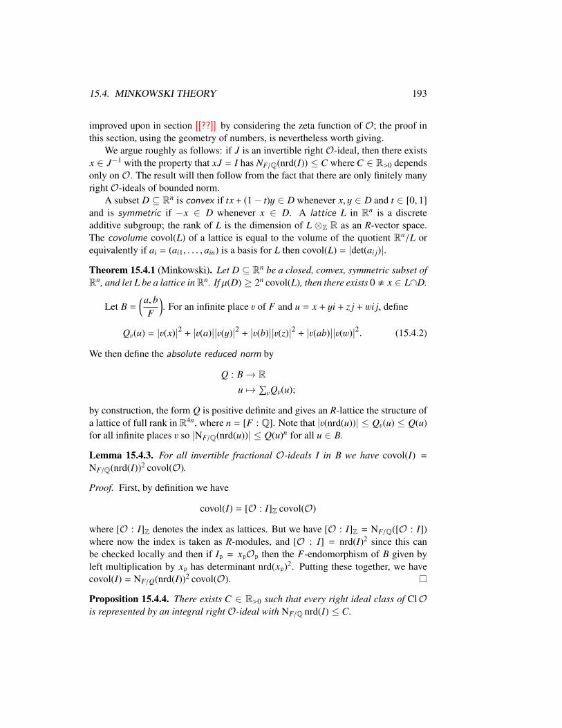
15.4. MINKOWSKI THEORY 193
improved upon in section [[??]] by considering the zeta function of O; the proof inthis section, using the geometry of numbers, is nevertheless worth giving.
We argue roughly as follows: if J is an invertible right O-ideal, then there existsx ∈ J−1 with the property that xJ = I has NF/Q(nrd(I)) ≤ C where C ∈ R>0 dependsonly on O. The result will then follow from the fact that there are only finitely manyright O-ideals of bounded norm.
A subset D ⊆ Rn is convex if tx + (1− t)y ∈ D whenever x, y ∈ D and t ∈ [0, 1]and is symmetric if −x ∈ D whenever x ∈ D. A lattice L in Rn is a discreteadditive subgroup; the rank of L is the dimension of L ⊗Z R as an R-vector space.The covolume covol(L) of a lattice is equal to the volume of the quotient Rn/L orequivalently if ai = (ai1, . . . , ain) is a basis for L then covol(L) = |det(ai j)|.
Theorem 15.4.1 (Minkowski). Let D ⊆ Rn be a closed, convex, symmetric subset ofRn, and let L be a lattice inRn. If µ(D) ≥ 2n covol(L), then there exists 0 , x ∈ L∩D.
Let B =
(a, bF
). For an infinite place v of F and u = x + yi + z j + wi j, define
Qv(u) = |v(x)|2 + |v(a)||v(y)|2 + |v(b)||v(z)|2 + |v(ab)||v(w)|2. (15.4.2)
We then define the absolute reduced norm by
Q : B→ Ru 7→ ∑
vQv(u);
by construction, the form Q is positive definite and gives an R-lattice the structure ofa lattice of full rank in R4n, where n = [F : Q]. Note that |v(nrd(u))| ≤ Qv(u) ≤ Q(u)for all infinite places v so |NF/Q(nrd(u))| ≤ Q(u)n for all u ∈ B.
Lemma 15.4.3. For all invertible fractional O-ideals I in B we have covol(I) =
NF/Q(nrd(I))2 covol(O).
Proof. First, by definition we have
covol(I) = [O : I]Z covol(O)
where [O : I]Z denotes the index as lattices. But we have [O : I]Z = NF/Q([O : I])where now the index is taken as R-modules, and [O : I] = nrd(I)2 since this canbe checked locally and then if Ip = xpOp then the F-endomorphism of B given byleft multiplication by xp has determinant nrd(xp)2. Putting these together, we havecovol(I) = NF/Q(nrd(I))2 covol(O).
Proposition 15.4.4. There exists C ∈ R>0 such that every right ideal class of ClOis represented by an integral right O-ideal with NF/Q nrd(I) ≤ C.

194 CHAPTER 15. CLASSES OF QUATERNION IDEALS
Proof. Let J be an invertible right fractional O-ideal. Then
covol(J−1) = N nrd(J)−2 covol(O).
Let D be the convex body {x ∈ R4n : Q(x) ≤ 1}, and let a > 0 be such that
a4n vol(D) = 24n covol(J−1) = 24n N nrd(J)−2 covol(O).
By Minkowski’s theorem, there exists 0 , x ∈ J−1 ∩ aD. Therefore
|NF/Q(nrd(x))|1/n ≤ Q(x) ≤ a2.
Consequently
N nrd(xJ)2 = |N nrd(x)|2 N nrd(J)2 ≤ a4n N nrd(J)2
= 24n covol(O) vol(D)−1 = C2.
Since x ∈ J−1, the ideal xJ = I is an O-ideal in the same ideal class as J, whichcompletes the proof.
Lemma 15.4.5. For any fractional ideal a of R, there are only finitely many rightO-ideals with nrd(I) = a.
Proof. We may assume a ⊆ R. Since nrd(I) = a we see that aO ⊆ I ⊆ O. ButO/aO is a finite set, so there only finitely many possibilities for I.
[[Cite Markus]][[This is like an “almost Euclidean algorithm”, analogous to the class group
of a number field. The pigeonhole principle should work, too.]]
15.5 Extensions and further reading
15.5.1. Cox [Cox89, §7] discusses orders in quadratic fields and the connections toquadratic forms and class numbers.
15.5.2. The composition law on binary quadratic forms can be understood quite con-cretely using 2× 2× 2 Rubik’s cubes, by a beautiful result of Bhargava [[cite]].
[[Manjul and Melanie take a different approach, and consider oriented quadraticrings and ideal classes. Is this really any different?]]
Remark 15.5.3. The notation Picent(O) is also used for PicZ(O)(O) where Z(O) isthe center ofO and we considerO as a Z(O)-algebra [[reference a remark on ordersover rings that are not domains]].
15.5. EXTENSIONS AND FURTHER READING 195
Exercises
Unless otherwise specified, throughout these exercises let R be a domain with fieldof fractions F, let V be an F-vector space, and let B be an F-algebra.
[[Some explicit computations.]]
15.1.


Chapter 16
Quaternion orders over Dedekinddomains
In this section, we begin to classify orders over a Dedekind domain.
16.1 Classifying orders
Let B be a quaternion algebra over Q. A maximal order in B is analogous to the ringof integers in a number field, but because of noncommutativity, maximal orders in Bare not unique (and in general, not unique even up to conjugation in B). Restrictingour investigations to maximal orders would come at a cost, as many natural ordersare not maximal: even the Lipschitz order quaternions Z+Zi +Z j +Zk, which ariseswhen considering if a positive integer is the sum of four squares, is not maximal,contained inside the Hurwitz order Z + Zi + Z j + Z(1 + i + j + k)/2.
How do we classify quaternion orders? In Chapter 4 (see Theorem 4.4.5), wesaw that quaternion algebras over a field F (with char F , 2) are classified by ternaryquadratic forms over F. It should come as no surprise, then, that quaternion ordersover a Dedekind domain R are classified by ternary quadratic modules over R (The-orem 16.3.1). The “module” part of this statement account for the possibility that Rmay not be a PID, and so some aspects of the class group of R creep in. Over Z, wehave an especially simple statement:
Theorem 16.1.1. There is a discriminant-preserving bijection{Quaternion orders over Zup to isomorphism
}←→
{ Nonsingular ternary quadratic forms over Zup to sign under the action of GL3(Z)
}where GL3(Z) acts on quadratic forms by the natural change of variable.
197

198 CHAPTER 16. QUATERNION ORDERS OVER DEDEKIND DOMAINS
The bijection is defined by restricting the reduced norm, as follows. Let O ⊂ Bbe a quaternion order over Z with reduced discriminant D = D(O) ∈ Z, a quantitywell defined up to sign. Let 1, i, j, k be a Z-basis for O: we do not assume that theseare standard generators! Let 1
2 , i], j], k] be the dual basis with respect to the standard
bilinear form α, β 7→ trd(αβ), arising from the reduced norm. So,
trd(i]) = 0, trd(ii]) = 1, trd(i j]) = trd(ik]) = 0, etc.
We then associate to O the quadratic form
Q(x, y, z) = D nrd(xi] + y j] + zk]),
defined up to sign. This quadratic form has discriminant D.Conversely, to the quadratic form Q
Q(x, y, z) = ax2 + by2 + cz2 + uyz + vxz + wxy ∈ Z[x, y, z]
up to sign, we associate the quaternion order O with basis 1, i, j, k where
i2 = ui− bc jk = ai = a(u− i)
j2 = v j− ac ki = b j = b(v− j)
k2 = wk − ab i j = ck = c(w− k);
(16.1.2)
this quaternion order has reduced discriminant
D = disc(Q) = 4abc− uvw− au2 − bv2 − cw2 , 0,
defined up to sign. (Note that if we scale the quadratic form by−1, the multiplicationlaws (16.1.2) do not change!) Completing the square, since Q is nonsingular, we seethat at least one of the discriminants
u2 − 4bc, v2 − 4ac, w2 − 4ab
is nonzero; assuming w2 − 4ab , 0, we have
O ⊂ B =
(w2 − 4ab, aDQ
)as well as the others by symmetry (when they apply).
The formulas may seem a little involved, so it is clarifying to work out the diag-
onal case. Let B =
(b, aQ
)(the interchange is deliberate!), and let
O = Z + Zi + Z j + Zk ⊂ B

16.1. CLASSIFYING ORDERS 199
be the tame order generated by the standard generators with
i2 = a, j2 = b, k = i j = − ji, k2 = −ab.
Then O has reduced discriminant D = −4ab. The dual basis is
i] = − i2b, j] = − j
2a, k] =
k2ab
and the reduced norm on this basis is
D nrd(xi] + y j] + zk]) = −4ab(−b4b2 x2 +
−a4a2 y
2 +ab
4(ab)2 z2)
= ax2 + by2 − z2.
Conversely, to the quadratic form Q(x, y, z) = ax2 + by2 − z2, we recover the orderZ + Zi + Z j + Zk with multiplication (16.1.2) by taking u = v = w = 0 and c = −1.
Why not just take the reduced norm restricted to the trace zero sublattice O0 ofO? In general, taking the trace zero subspace is not a good thing to do with respectto the prime 2. For example, we cannot recover O from its trace zero subspace: theLipschitz and Hurwitz orders both have trace zero subspace spanned by i, j, k. Thesecond more serious problem is that taking the trace zero quadratic form does notpreserve discriminants: for the tame order, we have Q(x, y, z) = nrd(xi + y j + zk) =
−bx2−ay2 + abz2 of discriminant 4(ab)2, not 4ab. We could recover the above formby taking instead
−(ab)−1Q(ax, by, z) =a2bx2 + ab2y2 − abz2
ab= ax2 + by2 − z2,
but this change of variables is achieved by taking the dual basis above, in a morenatural way!
Just as in the case of fields, the translation from quaternion orders to ternaryquadratic forms makes the classification problem potentially easier: we replace thepotentially complicated notion of finding a lattice closed under multiplication in aquaternion algebra with the simpler notion of choosing coefficients of a quadraticform. Using the local-global correspondence, in the next chapter, we tackle the clas-sification problem for ternary quadratic forms over a local ring, where we can bequite explicit.
However, before we do so, we take a tour of the zoo of orders and identify thosewith good properties. To start, recall that a Dedekind domain R is a (commutative)domain that is hereditary : every submodule of a projective module is again pro-jective. (Hence the name: projectivity is inherited by a submodule.) A domain ishereditary if and only if every ideal of R is projective, or equivalently, that any sub-module of a free R-module is a direct sum of ideals of R. This property is used in

200 CHAPTER 16. QUATERNION ORDERS OVER DEDEKIND DOMAINS
the proof of unique factorization of ideals and makes the structure theory of modulesover a Dedekind quite nice. (Note, however, that any order which is not maximal ina number ring is not hereditary.)
This definition carries over to the quaternionic context: an orderO is right hered-itary if every right ideal of O is projective as a right O-module. The standard invo-lution turns a right ideal into a left ideal, and so right hereditary is equivalent to theobvious notion of left hereditary, and so we simply refer to an order as hereditary.
There is a simple numerical criterion to test if an order is hereditary.
Theorem 16.1.3. A Z-orderO is hereditary if and only if discrd(O) is squarefree; inparticular, a maximal order O is hereditary.
Orders O with squarefree discriminant are easily described, via their comple-tions: they are orders of elements that are upper triangular modulo p for a finite setof primes p - disc(B). More precisely, let B be a quaternion algebra of discriminantD and let O(1) be a maximal order in B, so discrd(O(1)) = D. Let N be a squarefreeinteger coprime to disc(B), and let O ⊆ O(1) be an order with squarefree discrimi-nant discrd(O) = DN. Then at all primes p - N, we have Op = O(1)p is maximal.For the primes p | N, there exists an isomorphism O(1)p � M2(Zp) such that
Op =
{(a bpc d
): a, b, c, d ∈ Zp
}⊂ M2(Zp).
We can combine these into one, and write simply
ON �
{(a b
Nc d
): a, b, c, d ∈ ZN
}⊂ M2(ZN)
where ZN �∏
p|N Zp is the completion at N.More generally, Eichler considered those orders for which
ON �
{(a b
Nc d
): a, b, c, d ∈ ZN
}for an integer N coprime to D but not necessarily squarefree: these orders are calledEichler orders . Equivalently, an Eichler order is the intersection of two maximal or-ders. From the perspective of matrices, these are those which are not endomorphismsof a full rank 2 module but preserve an incidence modulo N.
There is one final way of classifying rings that extends nicely to the noncommuta-tive context. By way of analogy, note that orders in quadratic fields are characterizedsimply by their conductor. Let K = Q(
√D), where D ∈ Z is a fundamental discrim-
inant. Then the maximal order in K is Z +Zw where w = (D +√
D)/2. Any order S

16.2. QUADRATIC MODULES OVER RINGS 201
in K is of the form Z + f S = Z + Z fw, where f ∈ Z≥1 is the conductor of S , andthe discriminant of S is d = f 2D. Even in classical considerations, these orders arisenaturally when considering binary quadratic forms of nonfundamental discriminant.The condition that f = 1, which ensures maximality, also ensures that the dual isprojective, in other words, that S is Gorenstein. Gorenstein rings are natural from alinear algebra point of view.
An order O is Gorenstein if its dual O] is projective as a right O-module. In asimilar way, to a Z-order O ⊂ B, there is a unique maximal integer f = f (O) ∈ Z≥1such that O = Z + fO′ where O′ ⊂ B is a superorder of O. We call f the conductorof the order; it is also sometimes called the Brandt invariant after Brandt. An orderis Gorenstein if and only if f = 1. An Eichler order is Gorenstein, but there areGorenstein orders that are not Eichler. If O = Z + fO′ where f = f (O) is theconductor of O, then we call O′ ⊇ O the Gorenstein closure of O. To understandorders, therefore, it is enough to understand Gorenstein orders. In the language ofquadratic forms, an order is Gorenstein if and only if its associated quadratic form isprimitive, meaning the greatest common divisor of its coefficients is 1. Because ofthe importance of the Gorenstein property, we say that an order O is Bass if everyorder that contains O is Gorenstein.
To summarize, we have
maximal =⇒ hereditary =⇒ Eichler =⇒ Bass =⇒ Gorenstein
and each of these implications is strict.Finally, for a number ring R there is an ideal d of R called the different whose
norm is the discriminant; the different has better behavior under base extension.(There is probably some intrinsic geometric thing that the different measures.) Givethe basic review; over quadratic fields, the different is just the difference between thesquareroots.
In a same way, we define the different of a quaternion order D(O), a two-sidedideal. [[It is also just the commutator of the order, at least for a nice enough classof orders?]]
16.2 Quadratic modules over rings
To begin, we consider the theory of quadratic modules; this generalizes the theoryof quadratic forms in Section 8.6 by keeping track of the codomain (target) of thequadratic map.
Let R be a (commutative) noetherian domain with field of fractions F.
Definition 16.2.1. A quadratic map is a map Q : M → N between R-modules,satisfying:

202 CHAPTER 16. QUATERNION ORDERS OVER DEDEKIND DOMAINS
(i) Q(rx) = r2Q(x) for all r ∈ R and x ∈ M; and
(ii) The map T : M × M → N defined by
T (x, y) = Q(x + y)− Q(x)− Q(y)
is R-bilinear.
The map T in (ii) is called the associated bilinear map.A quadratic module over R is a quadratic map Q : M → L where M is a
projective R-module of finite rank and L is an invertible R-module. A quadraticform over R is a quadratic module with L = R.
Example 16.2.2. Let Q : V → F be a quadratic form. Let M ⊆ V be an R-lattice such that Q(M) ⊆ L where L is an invertible R-module. Then the restrictionQ|M : M → L is a quadratic module over R.
Conversely, if Q : M → L is a quadratic module over R, then the extensionQ : M ⊗R F → L⊗R F � F is a quadratic form over F.
Example 16.2.3. If Q : M → L is a quadratic module and c ⊆ R is a projectiveR-ideal, then Q extends naturally by property (i) to a quadratic module aM → a2L.
Definition 16.2.4. A similarity between quadratic modules (M, L,Q) and (M′, L′,Q′)is a pair of R-module isomorphisms f : M ∼−→ M′ and g : L ∼−→ L′ such thatQ′( f (x)) = g(Q(x)) for all x ∈ M, i.e., such that the diagram
MQ //
fo��
L
o g��
M′Q′ // L′
commutes. An isometry between quadratic modules is a similarity with L = L′ andg the identity map.
Remark 16.2.5. Similarity and isometry are different notions of “isomorphism” forquadratic modules where either you are allowed to move the codomain or not.
A similarity is a uniform These are just different notions of isomorphism, de-pending on if you can move the target or not. The notion of “isometry” comes fromthe connection with measuring lengths.
Think of a similarity like in the quaternion algebra case, where we can post mul-tiply by any nonzero element of the field and we get an isomorphic conic. This maychange the values of the quadratic form: q(x) and uq(x) are similar but not necessarilyisometric.
If free, then the same theory works fine.Discriminant, odd and even dimensions.

16.3. CONNECTION WITH TERNARY QUADRATIC FORMS 203
16.3 Connection with ternary quadratic forms
In this section, we classify quaternion orders over R in terms of ternary quadraticmodules, due to Brzezinski. There is a further connection with quaternary forms, butthis is for ideals; see the next section.
There are actually two different ways of doing it. I would
attribute them to the authors as follows.
The one of Brandt/Eichler/Peters/Brzsinski which rescales
the lattice by nr(L)ˆ-1 in the definition of O(L). This way
O(L)=O(aL) for each fractional ideal a. This works for any
Dedekind ring and induces bijections between similarity
classes of forms and isomorphism classes of Gorenstein orders.
The other one used by Pall/Nipp/Lemurell. Their definition of
O(L) does not use the factor nr(L)ˆ-1.
Over a PID this induces a bijection between similarity classes
of forms and isomorphism classes of arbitrary orders.
There is a very detailed description by Shimura that works out
the image of this second map over non PIDs.
We return to the notation we have used throughout this section (except the previ-ous one, where we allowed more generality): let R be a Dedekind domain with fieldof fractions F and let O be an R-order in a quaternion algebra B over F.
Theorem 16.3.1. There is a discriminant-preserving bijection between quaternionorders O over R and twisted isometry classes of ternary quadratic modules over Rwith nonzero discriminant.
We can be more specific; it’s also functorial.Let O] ⊂ B be the dual of O. Then
(O])0 = O] ∩ B0 = {α ∈ O] : trd(α) = 0}
is projective (locally free) of rank 3 so projective. We associate to O the quadraticmap Q(O) = nrd : O] ∩ B0 → d−2. [[This should be the same thing as taking theinverse different!]]
Remark 16.3.2. Over a field, this is the same. See also Lucianovic’s thesis. Over oddcharacteristic fields this makes no difference.
Lemma 16.3.3. Q(O) is a quadratic module.

204 CHAPTER 16. QUATERNION ORDERS OVER DEDEKIND DOMAINS
Proof.
Compute an explicit representation when free. Check morphisms (similarity).
Example 16.3.4. The Clifford functor respects morphisms of quadratic spaces butthe inverse does not. In particular, maximal quadratic spaces do not correspond tomaximal orders: the correspondence is only in one direction. There’s a specificexample where bad things happen at 2, but the problem is more general than that.
To show we get a bijection, we work in reverse. Let M = a1e1 ⊕ a2e2 ⊕ a3e3 andI = R and the quadratic form Q : M → R by
Q(xe1 + ye2 + ze3) = Q(x, y, z) = ax2 + by2 + cz2 + uyz + vxz + wxy, (16.3.5)
with a, b, c, u, v, w ∈ R. We just write down an algebra:
B = R⊕ Ri⊕ R j⊕ Rk
with multiplication laws
i2 = ui− bc jk = ai = a(u− i) k j = j k = −vw + ai + w j + vk
j2 = v j− ac ki = b j = b(v− j) ik = k i = −uw + wi + b j + uk (Q)
k2 = wk − ab i j = ck = c(w− k) ji = i j = −uv + vi + u j + ck
Check various things (exercise). This construction has been attributed to Eichler andappears in Brzezinski [Brz83] in the case R = Z. In this association, the reversal mapcorresponds to the standard involution on B.
Remark 16.3.6. In fact, this is the Clifford algebra of M.
Proof. Finish proof.
OK, now to read off invariants.
Proposition 16.3.7. If Q′ = bQ then b(O′) = bb(O). In particular, if Q is primitivethen b(O′) = (b) and G(O′) = O.
Remark 16.3.8. Relationship to the discriminant quadratic form.
Musing: is there any relationship to representation numbers for this form? E.g.splitting?

16.4. HEREDITARY ORDERS 205
16.4 Hereditary orders
Definition 16.4.1. An order O is hereditary if every right fractional O-ideal is in-vertible.
[[Nope! Hereditary is for one-sided ideals. Unless these are related?]]
16.4.2. Let O ⊆ B be a maximal order. Then I ⊆ O is a (maximal) invertibletwo-sided ideal if and only if Ip is so for all primes p.
We have two cases: either Bp � M2(Fp) or Bp is a division ring. In the formercase, we have that Op � M2(Rp) and Ip = M2(ap) = apM2(R) for some ap ⊆ Rp,and such an ideal is principal since ap is. If Bp is a division ring, then all (two-sided)ideals of the maximal orderOp are generated by a power of the unique maximal idealPp which is also principal.
Thus, all two-sided fractional O-ideals are locally principal, so O is hereditary,and the group of invertible two-sided fractional O-ideals is generated by {Pp ∩ O :p ramified in B} ∪ {pO : p ⊆ R prime}.
[[Same with ideal classes?]]
Definition 16.4.3. Let P be a two-sided integral O-ideal and suppose P , O. Wesay that P is prime if IJ ⊆ P implies I ⊆ P or J ⊆ P, where I and J are two-sidedintegral O-ideals.
Theorem 16.4.4. Suppose thatO is hereditary. Then the set of two-sided (invertible)fractional O-ideals of B forms an abelian group under multiplication, generated bythe prime ideals.
Proof. Let I be a two-sided integral O-ideal. Then since O is a finitely generatedR-module and R is noetherian, we conclude that I is contained in a proper maximal(integral)O-ideal M. From I ⊆ M we conclude that IM−1 ⊆ O, so IM−1 is integral.But nrd(IM−1) = nrd(I)/ nrd(M) | nrd(I). It follows that I can be written as theproduct of maximal ideals M by induction (on the reduced norm).
We will now show that in fact a maximal O-ideal is prime. For suppose thatIJ ⊆ M and that I * M. Then I + M is a two-sided O-ideal strictly containing M soI + M = O. But then J = IJ + MJ ⊆ M. Conversely, if P is prime and P ⊆ I whereI is a proper two-sided integral O-ideal, then P = I(I−1P), but I−1P ⊆ P impliesI−1 ⊆ O which is impossible so I ⊆ P hence P = I.
To conclude, we show that this group is abelian. Let P,Q be prime ideals. ThenPQ ⊆ P, so as above PQP−1 is integral, say PQP−1 = Q′. If Q′ = O then Q = O,a contradiction. But then choosing 0 , p ∈ P ∩ R then Q = pQp−1 ⊆ Q′, but Q ismaximal so Q = Q′. Thus PQ = Q′P, so the group is abelian.

206 CHAPTER 16. QUATERNION ORDERS OVER DEDEKIND DOMAINS
16.5 Eichler orders
An Eichler order is the intersection of two maximal orders, and it is this class oforders which we will study throughout. The level of an Eichler order O is the idealN ⊆ R satisfying d = DN; the level N is coprime to the discriminant D of B. Alter-natively, given a maximal order O ⊆ B, an ideal N coprime to D and an embeddingιN : O ↪→ M2(ZF,N) where ZF,N denotes the completion of ZF at N, an Eichler orderof level N is given by
O0(N) = {γ ∈ O : ιN(γ) is upper triangular modulo N} , (16.5.1)
and all Eichler orders arise in this way up to conjugation. In particular [Rei03, Theo-rem 39.14], an order O is hereditary (all one-sided ideals of O are projective) if andonly if O is an Eichler order with squarefree level.
Being Eichler is a local condition.Two orders O,O′ are conjugate (also isomorphic or of the same type) if there
exists ν ∈ B∗ such that O′ = ν−1Oν, and we write O � O′.
Proposition 16.5.2 ([Vig80, Corollaire III.5.5]). The number of isomorphism classesof Eichler orders O ⊆ B of level N is finite.
16.6 Gorenstein orders
Definition 16.6.1. O is Gorenstein if O] = Hom(O,R) = {α ∈ B : trd(αO) ⊆ R}[[why is this equivalent?]] is projective as a (left or) right O-module.
Lemma 16.6.2. O is Gorenstein if and only if Op is Gorenstein for all primes p.
Let O be an order.
Proposition 16.6.3. There exists a unique Gorenstein order G(O) ⊂ O and a uniqueideal b(O) ⊂ R such that
O = R + b(O)G(O).
Proof.
Lemma 16.6.4. We have O � O′ if and only if b(O) = b(O′) and G(O) � G(O′).
Proof.
Explicit example (Santi Molina).

16.7. DIFFERENT 207
16.7 Different
As in the commutative case, the discriminant can be realized as the norm of thedifferent, which here is two-sided and invertible.
Let B be a separable F-algebra and let I be an R-lattice in B.
Definition 16.7.1. The dual of I is
I] = {α ∈ B : trd(αI) = trd(Iα) ⊆ R}.
In particular, we have trd(I]I) ⊆ R.
16.7.2. I] is an R-lattice in B (Exercise 13.8). Clearly, if I ⊆ J then I] ⊃ J]. For allβ ∈ B× we have (βI)] = I]β−1.
16.7.3. We have I ⊆ (I])], since if α ∈ I and β ∈ I] then trd(αβ) ⊆ R so α ∈ (I])].
Lemma 16.7.4. We haveOR(I) ⊆ OL(I]) ⊆ OR((I])]), so equality holds if I = (I])].
Of course, a similar statement holds in Lemma 16.7.4, interchanging left andright.
Proof. Let α ∈ OR(I); then Iα ⊆ I, so I]Iα ⊆ I]I so
trd(αI]I) = trd(I]Iα) ⊆ trd(I]I) ⊆ R
hence αI] ⊆ I] and α ∈ OL(I]). Conversely, if α ∈ OL(I]) so αI] ⊆ I], then(αI])] = (I])]α−1 ⊇ (I])] so (I])] ⊇ (I])]α and α ∈ OR((I])]).
Now let O be an R-order.
Definition 16.7.5. We define the different of O to be O∗ = (O : O])L = (O : O])R.
[[Would Lenstra use a † here? What is ((O)])]?]]
Lemma 16.7.6. We have O∗ is a two-sided integral ideal of O with nrd(O∗)2 =
disc(O).
In particular, we may define the reduced discriminant of O to be discrd(O) =
nrd(O∗) and this agrees with the definition in the quaternion case.

208 CHAPTER 16. QUATERNION ORDERS OVER DEDEKIND DOMAINS
16.8 Other orders
Definition 16.8.1. An order is Bass if every order O′ ⊇ O is Gorenstein.
Gorenstein is weaker than Bass is weaker than Eichler is weaker than hereditaryis weaker than maximal.
Lemma 16.8.2. O is Bass if and only if Op is Bass for all primes p.
Finally, Eichler introduced a class of orders. Eichler
Definition 16.8.3. An order O is primitive if it contains a maximal R-order of aquadratic subfield of B.
Lemma 16.8.4. A primitive order is a Bass order.
Proof.
Is every Bass order primitive? True in the local case and for rational orders
Lemma 16.8.5. O is primitive if and only if Op is primitive for all primes p of R.
Proof. Local global.
16.9 Extensions and further reading
Condition (ii) can be given purely in terms of Q
Q(x + y + z) = Q(x + y) + Q(x + z) + Q(y + z)− Q(x)− Q(y)− Q(z)
for all x, y, z ∈ M.
16.9.1. In some lattice contexts, with R a Dedekind domain, a quadratic form withvalues in a fractional ideal a is called an a-modular quadratic form. Given the over-loaded meanings of the word modular, we do not employ this terminology. In thegeometric context, a quadratic module is called a line-bundle valued quadratic form.Sometimes called a-modular quadratic form or something. Sometimes you just wantto keep track of where the image lies.
First construction is due to Brandt clarified by Peters and generalizing a result ofLatimer General form due to Brandt Lemurell (also writing under the previous familyname Johansson), discusses the relationship between quaternion algebras and ordersand ternary quadratic forms [Lem11]. Also consult history in Gross and Lucianovic.
For more on quadratic forms over rings, see O’Meara, Knus, Scharlau, ...Other treatment by Gross and Lucianovic. Most general theorem is work of the
author [Voi11a].
16.9. EXTENSIONS AND FURTHER READING 209
Exercises
16.1. Finite intersection of maximal orders?
16.2. Let E be a field and let A be a F a finite extension of E [[Lassina’s exercise:there exists a Galois stable maximal order.]]
16.3. Prove the statement in Example 16.2.3. Conclude that up to similarity, thetarget of a quadratic module only depends on Pic(R)/2 Pic(R). Twisted dis-criminants.


Chapter 17
Quaternion orders over local PIDs
Carry out explicit local descriptions of all orders. Throughout, let F be a nonar-chimedean local field, R its ring of integers, p = (π) its maximal ideal, and k = R/pits (finite) residue field.
17.1 Eichler symbol
Let O be an R-order. We want to know if the order gives rise to a split, ramified, orinert extension of the residue field.
Let J(O) be the Jacobson radical of O.
Lemma 17.1.1. J(O) = O if and only if O � M2(R).
Proof. Exercise, using Wedderburn.
Suppose now that J(O) , O; then J(O) ⊇ pO and O/J(O) is a semisimplek-algebra, and hence a product of fields.
Exercise: only three possibilities.Accordingly, we make the following definition.
Definition 17.1.2. Define the Eichler symbol
e(O) =
1, if J(O) = R or O/J(O) � k × k;0, if O/J(O) � k;−1, if O/J(O) is a quadratic field extension of k.
.
Remark 17.1.3. Recall the definition of the discriminant quadratic form (Remark16.3.8). Then: e(O) = 0 if and only if ∆ is identically zero modulo p; and if ∆ is notidentically zero, then e(O) = 1 or −1 according as if
(∆(α)p
)= −1 for some α ∈ O.
211
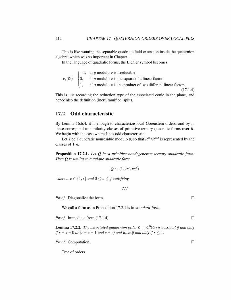
212 CHAPTER 17. QUATERNION ORDERS OVER LOCAL PIDS
This is like wanting the separable quadratic field extension inside the quaternionalgebra, which was so important in Chapter ...
In the language of quadratic forms, the Eichler symbol becomes:
ep(O) =
−1, if q modulo p is irreducible0, if q modulo p is the square of a linear factor1, if q modulo p is the product of two different linear factors.
(17.1.4)This is just recording the reduction type of the associated conic in the plane, andhence also the definition (inert, ramified, split).
17.2 Odd characteristic
By Lemma 16.6.4, it is enough to characterize local Gorenstein orders, and by ...these correspond to similarity classes of primitive ternary quadratic forms over R.We begin with the case where k has odd characteristic.
Let ε be a quadratic nonresidue modulo p, so that R×/R×2 is represented by theclasses of 1, ε.
Proposition 17.2.1. Let Q be a primitive nondegenerate ternary quadratic form.Then Q is similar to a unique quadratic form
Q ∼ 〈1, uπe, vπ f 〉
where u, v ∈ {1, ε} and 0 ≤ e ≤ f satisfying
???
Proof. Diagonalize the form.
We call a form as in Proposition 17.2.1 is in standard form.
Proof. Immediate from (17.1.4).
Lemma 17.2.2. The associated quaternion order O = C0(Q) is maximal if and onlyif r = s = 0 or (r = s = 1 and v = ε) and Bass if and only if r ≤ 1.
Proof. Computation.
Tree of orders.

17.3. EVEN CHARACTERISTIC 213
17.3 Even characteristic
Atomic. Do explicitly for some cases like unramified extension of Z2 and totallyramified extension Z2[
√2]?
17.4 Extensions and further reading
Discussed by Lemurell [Lem11, §5].
Exercises
17.1. Let O be a local quaternion order. Show that if O is not a local Bass order,then e(O) = 0.
17.2. Prove Lemma 17.2.2.
17.3. Let Q be a ternary quadratic form in standard form and let O = C0(Q) be theassociated quaternion order. Then
e(O) = ±1 if and only if e = 0 and f ≥ 1 and (−u/p) = ±1.


Chapter 18
Zeta functions and the massformula
In this chapter, we introduce zeta functions of a quaternion order and use them toinvestigate the class number of a totally definite quaternion order.
18.1 Zeta functions of quadratic fields
Gauss, in his investigation of binary quadratic forms was led to conjecture that therewere finitely many imaginary quadratic orders of class number 1. There are manyapproaches to this problem, involving some beautiful and deep mathematics. Giventhat we want to prove some kind of lower bound for the class number in terms of thediscriminant, it is natural to seek an analytic expression for this class number: thisis provided by the analytic class number formula of Dirichlet, and it turns the classnumber problem of Gauss into a (still hard, but tractable) problem of estimation. Ina similar way, we may ask: what are the definite quaternion orders of class number1? The method to prove Dirichlet’s formula generalizes to quaternion orders as well,as pursued by Eichler in his mass formula.
In this chapter, we treat these topics in detail. To introduce the circle of ideas,let K = Q(
√d) be a quadratic field of discriminant d ∈ Z and let R be its ring of
integers. We encode information about the field K by its zeta function. Over Q, wewould consider the Riemann zeta function
ζ(s) =
∞∑n=1
1ns (18.1.1)
as the prototypical such function; this series converges for Re s > 1, by the compari-
215

216 CHAPTER 18. ZETA FUNCTIONS AND THE MASS FORMULA
son test. By unique factorization, we have an Euler product
ζ(s) =∏
p
(1− 1
ps
)−1
where the product is over all primes p. The function ζ(s) can be meromorphicallycontinued to the right half-plane Re s > 0 using the fact that the sum
ζ2(s) =
∞∑n=1
(−1)n
ns
converges for Re s > 0 and
ζ(s) + ζ2(s) = 21−sζ(s)
so thatζ(s) =
121−s − 1
ζ2(s)
and the right-hand side makes sense for any Re s > 0 except for possible poles where21−s = 1. For real values of s > 1, we have
1s− 1
=
∫ ∞
1
dxxs ≤ ζ(s) ≤ 1 +
∫ ∞
1
dxxs =
ss− 1
so1 ≤ (s− 1)ζ(s) ≤ s;
therefore, as s →+ 1, we have (s − 1)ζ(s) → 1, so ζ(s) has a simple pole at s = 1with residue ress=1 ζ(s) = 1.
For the field K, modeled after (18.1.1) we define the Dedekind zeta function by
ζK(s) =∑a⊆R
1N(a)s (18.1.2)
where the sum is over all nonzero ideals of R and the series is defined for Re s > 1.We can also write this as a Dirichlet series
ζK(s) =
∞∑n=1
an
ns
where an is the number of ideals of norm n in R. By unique factorization of ideals,we again have an Euler product expansion
ζK(s) =∏p
(1− 1
N ps
)−1
, (18.1.3)
the product over all nonzero prime ideals p ⊂ R.

18.2. IMAGINARY QUADRATIC CLASS NUMBER FORMULA 217
18.2 Analytic class number formula for imaginaryquadratic fields
In order to introduce a formula that involves the class number, we group the ideals in(18.1.2) by their ideal class: for [b] ∈ Cl(K), we define
ζK,[b](s) =∑a⊆R
[a]=[b]
1N as
so thatζK(s) =
∑[b]∈Cl(K)
ζK,[b](s). (18.2.1)
In general, for [b] ∈ Cl(K), we have [a] = [b] if and only if there exists a ∈ K× suchthat a = ab, but since a ⊆ R, in fact we have
a ∈ b−1 = {a ∈ R : ab−1 ⊆ R};
this gives a bijection{a ⊆ R : [a] = [b]} ↔ b−1/R×,
(since the generator of an ideal is unique up to units). Thus
ζK,[b](s) =1
N bs
∑0,a∈b−1/R×
1(N a)s . (18.2.2)
for each class [b] ∈ Cl(K).Everything we have done so far works equally as well for real as for imaginary
quadratic fields. But here, to make sense of b−1/R× in the simplest case, we wantR× to be a finite group, which means exactly that K is imaginary quadratic. So fromnow on this section, we assume d < 0. Then w = #R× = 2, except when d = −3,−4where w = 6, 4, respectively.
Under this hypothesis, the sum (18.2.2) can be transformed into sum over latticepoints with the fixed factor w of overcounting. Before estimating the sum over recip-rocal norms, we first estimate the count. Let Λ ⊂ C be a lattice. We can estimate thenumber of lattice points λ ∈ Λ with |λ| ≤ x by the ratio πx2/A, where A is the areaof a fundamental parallelogram P for Λ: roughly speaking, this says that we can tilea circle of radius x with approximately πx2/A parallelograms P.
More precisely, we have the following lemma.

218 CHAPTER 18. ZETA FUNCTIONS AND THE MASS FORMULA
Lemma 18.2.3. Let Λ ⊂ C be a lattice with coarea area(C/Λ) = A. Then there is aconstant C such that for all x > 1, we have∣∣∣∣∣∣#{λ ∈ Λ : |λ| ≤ x} − πx2
A
∣∣∣∣∣∣ ≤ Cx.
We leave this lemma as an exercise (Exercise 18.1) in tiling a circle with radiusx with fundamental parallelograms for the lattice Λ.
Now we apply this lemma to a lattice b−1 ⊂ C. We write
ζK,[b](s) =1
w(N bs)
∞∑b=1
bn
ns
wherebn = #{a ∈ b−1 : N a = n}.
Since N a = |a|2, for all x > 1 we have∑n≤x
bn = #{a ∈ b−1 : 0 < |a| ≤√
x};
from Lemma 18.2.3, we conclude∣∣∣∣∣∣∣∣∑n≤x
bn −πxA
∣∣∣∣∣∣∣∣ ≤ C√
x
where A is the coarea of b−1 and C is a constant that does not depend on x. Wecompute that
A = N(b−1)
√|d|2
.
Now consider the Dirichlet series
f (s) =1
w(Nb)s
∞∑n=1
(bn −
π
A
) 1ns .
Then the estimate ∣∣∣∣∣∣∣∣∑n≤x
(bn −
π
A
)∣∣∣∣∣∣∣∣ =
∣∣∣∣∣∣∣∣∑n≤x
bn −πxA
∣∣∣∣∣∣∣∣ ≤ C√
x
by the comparison test implies that f (s) converges for all Re s > 1/2 and in particularf (s) converges at s = 1. For s > 1, we have
f (s) = ζK,[b](s)− π
Aw(Nb)s ζ(s)

18.2. IMAGINARY QUADRATIC CLASS NUMBER FORMULA 219
so
ζK,[b](s) = f (s) +2π
w√|d|
(Nb)1−sζ(s).
hence
ress=1 ζK(s) = lims→+1
(s− 1)ζK,[b](s)
= lims→+1
(s− 1) f (s) +2π
w√|d|
lims→+1
(s− 1)(Nb)1−sζ(s)
= 0 +2π
w√|d|· 1 =
2π
w√|d|.
In particular, ζK,[b](s) has a simple pole at s = 1 with residue independent of [b].Summing the residues over [b] ∈ Cl(K), from (18.2.1) we have the following result.
Theorem 18.2.4 (Analytic class number formula for imaginary quadratic field). LetK = Q(
√d) be an imaginary quadratic field with discriminant d < 0. Let h be the
class number of K and w the number of roots of unity in K. Then
ress=1 ζK(s) =2πh
w√|d|.
This formula simplifies slightly if we cancel the pole at s = 1 with ζ(s), asfollows. Like in the Dirichlet series, we can combine terms in (18.1.3) to get
ζK(s) =∏
p
∏p|p
(1− 1
N ps
)−1
and
Lp(s) =∏p|p
(1− 1
N ps
)−1
=
(1− p−s
)−2, if (p) = pp′ splits in K;(
1− p−s)−1
, if (p) = p2 ramifies in K;(1− p−2s
)−1, if (p) is inert in K.
We condition of being split, ramified, or inert in K is recorded in a character:
χ(p) = χd(p) =
1, if p splits in K;0, if p ramifies in K;−1, if p is inert in K

220 CHAPTER 18. ZETA FUNCTIONS AND THE MASS FORMULA
for prime p and extended to all positive integers by multiplicativity. If p - d is an oddprime, then
χ(p) =
(dp
)is the usual Legendre symbol, equal to 1 or−1 according as if d is a quadratic residueor not modulo p. Then
Lp(s) = (1− p−s)(1− χ(p)p−s).
Expanding the Euler product term-by-term and taking a limit, we have
ζK(s) = ζ(s)L(s, χ) (18.2.5)
where
L(s, χ) =∏
p
(1− χ(p)
ps
)−1
=∑
n
χ(n)ns .
The function L(s, χ) is in fact holomorphic for all Re s > 0; this follows from thefact that the partial sums
∑n≤x χ(n) are bounded and the mean value theorem. So in
particular the series
L(1, χ) = 1 +χ(2)
2+χ(3)
3+χ(4)
4+ . . .
converges (slowly). Combining (18.2.5) with the analytic class number formulayields:
L(1, χ) =2πh
w√|d|.
For example, taking d = −4, so χ(2) = 0 and χ(p) = (−1/p) = (−1)(p−1)/2, we have
L(1, χ) = 1− 13
+15− 1
7+
19− 1
11+ · · · =
∏p≥3
(1− (−1)(p−1)/2
p
)−1
=π
4= 0.7853 . . . .
Remark 18.2.6. The fact that L(1, χ) , 0, and its generalization to complex char-acters χ, is the key ingredient to prove Dirichlet’s theorem on primes in arithmeticprogression (Theorem 11.2.8), used in the classification of quaternion algebras overQ. The arguments to complete the proof are requested in Exercise 18.8.4.
To approach the class number problem of Gauss, we would then seek lowerbounds on L(1, χ) in terms of the discriminant |d|. Rather than go into these esti-mates here, we refer to the additional reading in Paragraph 18.8.1.

18.3. EICHLER MASS FORMULA OVER THE RATIONALS 221
18.3 Eichler mass formula over the rationals
We are now prepared to consider the analogue of the above for quaternion orders.Let B be a quaternion algebra over Q and let O be a maximal order in B. We definethe zeta function of O to be
ζO(s) =∑I⊆O
1N(I)s , (18.3.1)
the sum over all nonzero right ideals in O. A maximal order is hereditary, so everyright ideal is projective hence locally principal (and invertible), and here we need notconcern ourselves with the subtler aspects of ideal theory as in Chapter 14.
Let an be the number of right ideals in O of reduced norm (n) for n > 0. ThenN(I) = nrd(I)2, so
ζO(s) =
∞∑n=1
an
n2s .
To establish an Euler product for ζO(s), we will give a kind of factorization formulafor right ideals of O, but by necessity, writing an ideal as a compatible product willinvolve the entire set of orders connected to O; in any case, we will show that amn =
aman whenever m, n are coprime. Next, we will count the ideals of a given reducednorm q = pe a power of a prime: the answer will depend on whether p is ramified ornot in B. As a result, we will find
ζO(s) =∏
p
ζO,p(s)
where
ζO,p(s) =
(1− p−2s
)−1, if p is ramified;(
1− p−2s)−1 (
1− p1−2s)−1
, if p is unramified.(18.3.2)
In particular, this formula shows that ζO(s) does not depend on the choice of maximalorder O, so we may also write ζB(s) = ζO(s). From (18.3.2), we have
ζO(s) = ζ(2s)ζ(2s− 1)∏p|D
(1− 1
p2s−1
)
where D > 0 is the discriminant of B. In particular, we have
ress=1 ζO(s) = lims→+1
(s− 1)ζO(s) =ζ(2)
2
∏p|D
(1− 1
p
)=π2
12
∏p|D
(1− 1
p
). (18.3.3)

222 CHAPTER 18. ZETA FUNCTIONS AND THE MASS FORMULA
(We could also look to cancel the poles of ζO(s) in a similar way to define an L-function, holomorphic for Re s > 0.)
Now we break up the sum (18.3.1) according to right ideal class:
ζO(s) =∑
[J]∈Cl(O)
ζO,[J](s)
whereζO,[J](s) =
∑I⊆O
[I]=[J]
1N(I)s .
Since [I] = [J] if and only if I = αJ for some invertible α ∈ J−1, and µJ = J if andonly if µ ∈ OL(J)×, we have
ζO,[J](s) =1
N(J)s
∑0,α∈J−1/OL(J)×
1N(α)s .
In order to proceed, we assume that B is definite (ramified at∞) or equivalentlythat #OL(J)× < ∞. Let wJ = #OL(J)/{±1}. We again argue by counting latticepoints to prove the following proposition.
Proposition 18.3.4. The function ζO,[J](s) has a simple pole at s = 1 with residue
ress=1 ζO,[J](s) =π2
wJD.
Rather than give a proof of this proposition (which will be proven in this chapterin greater generality), we only give a sketch of the idea. Using a Tauberian theorem,we will show that
ress=1 ζO,[J](s) =1
2wJ N(J)
vol(R4≤1)
covol(J)where
vol(R4≤1) = vol({x ∈ R4 : |x| ≤ 1}) = 2π2
and J ↪→ J⊗R � H � R4 has the structure of a lattice in R4 with covol(J) =
covol(O)/N(J) = D/N(J). Putting all of these facts together, we have
ress=1 ζO,[J](s) =2π2
2wJ N(J)N(J)
D=
π2
wJD.
Combining Proposition 18.3.4 with (18.3.3), we have
ress=1 ζO(s) =π2
D
∑[J]∈Cl(O)
1wJ
=π2
12
∏p|D
(1− 1
p
)and we conclude the following theorem.

18.4. ANALYTIC CLASS NUMBER FORMULA 223
Theorem 18.3.5 (Eichler mass formula). Let O be a maximal order in a definitequaternion algebra over Q of discriminant D. Then∑
[J]∈Cl(O)
1wJ
=φ(D)12
where wJ = #OL(J)/{±1} and φ is the Euler φ-function.
The Eichler mass formula does not quite give us a formula for the class number;rather, it gives us a formula for a “weighted” class number (we can think of wJ
as the order of the nonscalar automorphism group of J), and this is still useful forapplications.
Corollary 18.3.6. We have # Cl(O) = 1 if and only if D = 2, 3, 5, 7, 13.
Proof. We have # Cl(O) = 1 if and only if
1w
=φ(D)12
where w = #O/{±1}. For the cases D = 2, 3, we have seen already that the maximalorder O is fact Euclidean and w = 12, 6, respectively; this independently verifiesthe Eichler mass formula in these cases. We will see in Section 21.1 that if D > 3then w ≤ 3. By elementary arguments with the Euler φ function (Exercise 18.2), wehave φ(D)/12 = 1/w with w ≤ 3 only if D = 5, 7, 13, 42, and we can check each
discriminant in turn. For D = 5, we may take B =
(−5,−3Q
)and a maximal order
O containing Z[(−1 + j)/2], so w = 3 and # Cl(O) = 1. The other cases followsimilarly; the details are requested in Exercise 18.3.
In Section 18.6, we go farther and find all definite quaternion orders of classnumber 1, following Brzezinski.
18.4 Analytic class number formula
Let F be a number field with r real places and c complex places, so that [F : Q] =
n = r + 2c. Let R be the ring of integers in F. Define the Dedekind zeta function fors ∈ C with <(s) > 1 by
ζF(s) =∑a⊆R
1Nas =
∏p
(1− 1
Nps
)−1

224 CHAPTER 18. ZETA FUNCTIONS AND THE MASS FORMULA
where the sum is over all nonzero ideals of R, the product is over all primes of R, andNa is the absolute norm. Then ζF admits an analytic continuation to all of C with asimple pole at s = 1 with residue
ζ∗F(1) = lims→1
(s− 1)ζF(s) =2r1(2π)r2
w√
dFhFRegF (18.4.1)
where wF is the number of roots of unity in F, hF = # Cl R is the class number of F,RegF is the regulator of F, and dF is the absolute discriminant of F
More generally, for a ∈ Cwe write ζ∗F(a) for the leading coefficient in the Laurentseries expansion for ζF at s = a.
The formula (18.4.1) is known as Dirichlet’s analytic class number formula (eventhough Dirichlet’s theorem concerned quadratic forms rather than classes of ideals).Using the functional equation for ζF , we can also write this more simply as
ζ∗F(0) = lims→0
s−(r1+r2−1)ζF(0) =hFRegF
wF;
here, ζF has a zero at s = 0 of order r1 + r2 − 1.In the situation where F is an imaginary quadratic field (r1 = 0 and r2 = 1), we
have RegF = 1, so we find that
hF = wFζF(0)
and in particular if dF > 4 then hF = 2ζF(0).In brief, this formula is proved as follows. We write the Dedekind zeta function
as a sum over ideals in a given ideal class: we define the partial zeta function
ζF,[b](s) =∑a⊆R
[a]=[b]
1Nas
so thatζF(s) =
∑[b]∈Cl R
ζF,[b](s).
Now note that [a] = [b] if and only if a = ab for some nonzero
a ∈ b−1 = {x ∈ F : xb ⊆ R},
so we have a bijection between nonzero ideals a ⊆ R such that [a] = [b] and the setof nonzero elements in b−1/R×. So
ζF,[b](s) =1
Nbs
∑0,a∈b−1/R×
1|Na|s
.

18.5. ZETA FUNCTIONS OF QUATERNION ALGEBRAS 225
One now reduces to a problem concerning lattice points after choosing a fundamentaldomain for the action of R×, which reduces to a volume computation (an exercise inmultivariable integration with polar coordinates): one finds that
ζ∗F,[b](s) =2r1(2π)r2
w√
dFRegF
(independent of [b]!) and Dirichlet’s formula follows.
18.5 Zeta functions of quaternion algebras
We now mimic the above proof in our quaternionic setting.Recall from strong approximation that if F is a function field, or if F is a number
field and B satisfies the Eichler condition—i.e., that there is an unramified archime-dean place for B—then one may identify the class number of any order O ⊆ B witha suitable class group.
So only one case remains to consider. Let F be a totally real number field and letB be a quaternion algebra which is ramified at all real places of F; we say that B is a(totally) definite (and otherwise we say B is indefinite).
Remark 18.5.1. To extend the analogy, we also note that this situation is analogousto one without a regulator term (as would be necessary, as otherwise the unit groupswould be infinite and noncommutative!).
Let O be an order in B.Let I be an integral right O-ideal, so that I ⊆ O. We define N(I) = #(O/I). We
have N(I) = NF/Q nrd(I)2. For example, if a ⊆ R is a nonzero ideal then N(aO) =
NF/Qa4. Note this agrees with the covolume computation in Lemma 15.4.3.
We then define the zeta function of O to be
ζO(s) =∑I⊆O
1N(I)s =
∑n
anN(n)2s (18.5.2)
where the first sum is over all (nonzero) integral right O-ideals I and in the secondsum an is the number of right O-ideals I with nrd(I) = n.
Our first order of business is to establish an Euler product for ζO(s).
Lemma 18.5.3. Let I be an integral O-ideal with nrd(I) = ab and a and b coprime.Then I can be uniquely written as a compatible product I = I(a)I(b) with nrd(I(a)) =
a and nrd(I(b)) = b.
Proof. Let O′ = OL(I). Define I(a) = I + aO′ and I(b) = I + bO. The statementholds if and only if it holds locally, so let p be a prime of R. If p - ab then Ip = Op =

226 CHAPTER 18. ZETA FUNCTIONS AND THE MASS FORMULA
I(a)p = I(b)p. If p | a, then I(a) = Ip and I(b)p = Op and so nrd(I(a)p) = nrd(Ip) and(I(a)I(b))p = IpOp = Ip and the product is compatible. We have a similar statementfor p | b. The result follows.
If we factor an O-ideal into a product of ideals whose norms are powers of aprime, then these ideals will have orders which will be in general different than O.Of course, if O and O′ are connected (locally isomorphic) orders, then since idealscan be recovered from its localizations there is a bijection between the right ideals ofO and of O′ of any reduced norm a.
Suppose that O is hereditary. Then when we factor I into a product of ideals ofprime power norm, each left and right order that appears in the product is connectedto O, since each ideal is locally principal. It follows that if an is the number ofright O-ideals of norm an, then amn = aman whenever m and n are relatively prime.Consequently
ζO(s) =∏p
ζOp(s)
where
ζOp(s) =∑
Ip⊆Op
1N(Ip)s =
∞∑e=0
ape
Np2s .
We are now reduced to counting ideals locally.
Lemma 18.5.4. LetOp be a maximal order in Bp and let q = pe be a prime power ofR.
If p is ramified in B, then there is a unique (left or) right integralO-ideal of normq.
If p is unramified in B, then the number of (left or) right integral O-ideals ofnorm p is equal to 1 + Np + · · · + Npe.
Proof. If p is ramified then the unique maximal order Op has a unique (two-sided)maximal ideal P with nrd(P) = p and all ideals of Op are powers of P.
So suppose that p is split in B. Let Ip = xpOp be a right integralOp-ideal of normpe and let π be a uniformizer for p. Then we can write
xp =
(πe− f 0
r π f
)for unique f ∈ Z≥0 and r ∈ R/p f (Exercise 19.5. Since #R/p f = Np f , it followsthat the number of such ideals is equal to 1 + Np + · · · + Npe.
18.5. ZETA FUNCTIONS OF QUATERNION ALGEBRAS 227
From this lemma we have
ζOp(s) =
(1− 1
Np2s
)−1
if p is ramified, and
ζOp(s) =
∞∑e=0
1 + Np + · · · + Npe
Np2es =
(1− 1
Np2s
)−1 (1− 1
Np2s−1
)−1
if p is split.Recall that
ζF(s) =∏p
(1− 1
Nps
)−1
.
Thus
ζO(s) =∏p
ζOp(s) = ζF(2s)ζF(2s− 1)∏p | D
(1− 1
Np2s−1
)where D is the discriminant of B. (Here one needs to break up the sum into ideals ofnorm ≤ X and those > X and show that the product converges, etc.)
Since the ζF has only a simple pole at s = 1, there is a single simple pole of ζOat s = 1, and we conclude that
ζ∗O(1) = lims→1
(s− 1)ζO(s) =ζF(2)
2ζ∗F(1)
∏p|D
(1− Np−1). (18.5.5)
We now write ζO(s) as a sum over right ideal classes and analyze the residueat s = 1 by a volume a computation as with the analytic class number formula.Combining this with (18.5.5), we will obtain a mass formula for the order O.
For an integral right O-ideal J, let
ζO,[J](s) =∑I⊆O
[I]=[J]
1N(I)s .
Then obviouslyζO(s) =
∑[J]∈ClO
ζO,[J](s).
We have [I] = [J] if and only if I � J if and only if I = xJ for nonzero x ∈ J−1
(recall that B is a division ring since it is ramified at its real places). Since uJ = J ifand only if u ∈ OL(J)× (Exercise 19.7), it follows that
ζO,[J](s) =1
N(J)s
∑0,x∈J−1/OL(J)×
1N(x)s .

228 CHAPTER 18. ZETA FUNCTIONS AND THE MASS FORMULA
But nowOL(J)×/R× is finite since B is totally definite. Let w(J) = #OL(J)×/R×.Then
ζO,[J](s) =1
w(J)N(J)s
∑0,x∈J−1/R×
1N(x)s .
Proposition 18.5.6. ζO,[J](s) has a simple pole at s = 1 with residue
ζ∗O,[J](1) =2n(2π)2nRegF
8w(J)d2F ND
.
With this lemma in hand, we find that
ζ∗O(1) =2n(2π)2nRegF
8d2F ND
∑[J]∈ClO
1w(J)
=ζF(2)
2
(2n
2√
dFhFRegF
)∏p|D
(1− 1
Np
)since wF = 2 (F is totally real) so since D is squarefree we have∑
[J]∈ClO
1w(J)
= ζF(2)2
(2π)2n hFd3/2F
∏p|D
(Np− 1).
By the functional equation for ζF , we have
ζF(−1) =
(−12π2
)n
d3/2F ζF(2)
so we can also write ∑[J]∈ClO
1w(J)
= 21−n|ζF(−1)|hFΦ(D)
where we defineΦ(D) =
∏p|D
(Np− 1),
the generalization of Euler’s Φ-function. We have proven the following theorem.
Theorem 18.5.7 (Eichler’s mass formula). We have∑[J]∈ClO
1[OL(J)× : R×]
= 21−n|ζF(−1)|hFΦ(D).
Corollary 18.5.8. If O is the maximal order in a definite quaternion algebra of dis-criminant D over Q, then ∑
[J]∈ClO
1#OL(J)×
=124φ(D).

18.5. ZETA FUNCTIONS OF QUATERNION ALGEBRAS 229
In the (unlikely) situation where OL(J)× = u is independent of J, we wouldconclude that
# ClO = H = u21−n|ζF(−1)|hFΦ(D).
[[As an approximation, H is roughly d3/2F ND/2n.]]
Proof of Proposition 18.5.6. We first prove this statement in the case F = Q, sincethen we can see the main ideas minimizing technicalities. We will come back andtreat the general case. [[Sucker!]]
In this situation, our formula greatly simplifies and we need to show that ζO,[J](s)has a simple pole at s = 1 with residue π2/(w(J)D) where D is the discriminant of B.We have written
ζO,[J](s) =1
w(J)N(J)s
∑0,x∈J−1/{±1}
1N(x)s .
The key technical fact is the following. Let X ⊆ Rn be a cone and suppose0 < N(X). Suppose that X≤1 = X ∩ {x ∈ Rn : N(x) ≤ 1} is bounded and has volumevol(X≤1). Let L ⊆ Rn be a lattice of full rank in Rn and has covolume covol(L). Let
ζL,X(s) =∑
x∈X∩L
1N(x)s .
Then ζL,X(s) converges for Re s > 1 and has a simple pole at s = 1 with residue
ζ∗L,X(1) = lims→1+
(s− 1)ζL,X(s) =vol(X≤1)covol(L)
.
Whew! In our case, we consider the lattice
J−1 ↪→ B⊗Q R � H � R4.
The choice of sign allows us to choose the first coordinate to be positive, so we takeX = R≥0 × R3. We have vol(X) = 1/2(2π2) = π2. From the previous section onMinkowski theory, we have covol(J−1) = covol(O)/N(J). And almost by definitionwe have covol(O) =
√discO = D. Putting this together with the technical fact, we
have
ζ∗O,[J](1) = f rac1w(J)N(J)π2N(J)
D=
π2
w(J)D
as claimed.

230 CHAPTER 18. ZETA FUNCTIONS AND THE MASS FORMULA
18.6 Class number 1 problem
The list of all definite quaternion orders of class number 1 over the integers wasdetermined by Brzezinski [Brz95] in the language of ternary quadratic forms.
(
Theorem 18.6.1 (Brzezinski). There are 25 isomorphism classes of definite quater-nion orders over Z with class number 1.
Proof. Mass formula for maximal orders.
Also work with Markus.
It turns out
that there are no non-principal Euclidean ideal classes for maximal
Z-orders in definite rational quaternion algebras.
But the way things worked out was somewhat interesting: the class
number 2 (reduced) discriminants are 11, 17, 19, 30, 42, 70, 78.
For 11, 17, 19, it turns out that the type number is also 2. This
means that the Brandt groupoid has the following structure:
there are the two nonsiomorphic maximal orders, say O1 and O2. The
right Picard set [I think you might call this the "left Picard set in
your notes", and you might well be right; anyway you get the point] of
O1 consists of O1 together with an ideal I with left order O1 and
right order O2. Similarly, the right Picard set of O2 consists of O2
together with an ideal I’ with left order O2 and right order O1. Thus
in the Brandt groupoid I’ is the inverse of I, whereas O1 and O2 are
self-inverse.
[So the picture is a graph with two vertices and four oriented edges,
two of which are loops and a pair of mutually inverse edges running
between the two vertices.]
These four "arrows" in the groupoid represent three different
quadratic forms: an ideal and its inverse give rise to the same
quadratic form. In fact these three quadratic forms comprise a full
genus (I checked that independently on the quadratic lattice side).
Before I was looking only at one of the maximal orders and was very
confused as to why MAGMA was telling me that the class number of the
associated quadratic form was equal to 3. I think I get it now!
Note that this means that the two-sided Picard group of each of O1 and
O2 is trivial (in particular they are isomorphic!),

18.7. ZETA FUNCTIONS OVER FUNCTION FIELDS 231
and this means that if there is any Euclidean ideal class, then there
would be a Euclidean order, forcing the class number to be 1 rather
than 2. (Of course I checked this by computing the Euclidean minima
of the 3 forms in question: they are all bigger than 1, although not
tremendously so.)
For 30,42,70,78, it turns out that the type number is 1. So in this
case the Brandt groupoid is simply equal to the two-sided Picard
group, which has cardinality 2. In other words there is a unique
nonprincipal two-sided ideal, which is a candidate for being a
Euclidean ideal class...but it turns out not to be. (On the other
hand, I think I could invert a suitable small set of primes in Z in
such a way as to keep the class numbers, type numbers, etc. the same
but make the nonprincipal ideal class be Euclidean. I should probably
do that: it would be nice to have an actual example.)
You might want to use this example in your book. (Or you might not:
just a late night idea.)
Let me say that although obviously the first three discriminants have
one prime factor and the last four have three prime factors, in and of
itself this doesn’t explain to me why the two Picard groups have
different structures. I happen to know that the two-sided Picard
group is an elementary abelian two-group whose F_2-dimension is *at
most* the number of ramified primes, but that doesn’t explain
everything here: certainly there are examples of quaternion algebras
of prime discriminant with nontrivial two-sided Picard group, e.g. D =
73, 89. (If there is some clear answer as to when the Picard group
is trivial and when it has order 2 in the prime discriminant case, I
am not aware of it.)
Best regards,
Pete
18.7 Zeta functions over function fields
18.8 Extensions and further reading
18.8.1. Further reading for Gauss class number 1 problem.
18.8.2. Eichler mass formula and supersingular elliptic curves.

232 CHAPTER 18. ZETA FUNCTIONS AND THE MASS FORMULA
18.8.3. The primes p = 2, 3, 5, 7, 13 in Corollary 18.3.6 are also the primes p suchthat the modular curve X0(p) has genus 0. This is not a coincidence, and reflects adeep correspondence between classical and quaternionic modular forms.
18.8.4. Prove the theorem on primes in arithmetic progression (Theorem 11.2.8)using the nonvanishing L(1, χ) , 0 for characters χ, as follows.
18.8.5. More generally, we can replace the orthogonal group with another compact,semisimple Lie group G∞, an integral model for it GZ, and ask for the weighted sumof the class set of objects with automorphism group GZ. (For example, unitary groupand Hermitian lattices, symplectic group, G2, etc.) Weil conjectured a formula forthis in terms of a product, and Langlands, Lai, and Kottwitz proved general state-ments for number fields. The right way to formulate this is in terms of double cosets,where the final answer comes down to a Tamagawa number calculation.
The function field equivalent is a problem in topology.
Exercises
18.1. Prove Lemma 18.2.3 as follows.
a) Let P be a fundamental parallelogram for Λ, and for λ ∈ Λ let Pλ = P+λ.For x > 1, let D(x) = {z ∈ C : |z| ≤ x}, and
N(x) = #{λ ∈ Λ : λ ∈ D(x)}NP(x) = #{λ ∈ Λ : Pλ ⊆ D(x)}N+
P (x) = #{λ ∈ Λ : Pλ ∩ D(x) , ∅}.
Show thatN(x) ≤ NP(x) ≤ N+
P (x).
b) Show that NP(x) ≤ πx2/A ≤ N+P (x).
c) Let d be the length of a long diagonal in P. Show that for any λ ∈Λ ∩ D(x), we have Pλ ⊆ D(x + d), so
N(x) ≤ NP(x + δ) ≤ π(x + d)2
A.
Similarly, show that if Pλ ∩ D(x− d) then Pλ ⊆ D(x) and λ ∈ D(x), so
π(x− d)2
A≤ N+
P (x− d) ≤ N(x).

18.8. EXTENSIONS AND FURTHER READING 233
d) Conclude that Lemma 18.2.3 holds with C = π/A(2x + x2). See [Wes,Lemma 1.19].
18.2. Show that if D is a squarefree integer with an odd number of prime factorswith φ(D)/12 ∈ {1, 1/2, 1/3}, then D ∈ {5, 7, 13, 42}.
18.3. Using the explicit description of maximal orders, show that maximal ordersof discriminant D = 5, 7, 13 have class number 1 and a maximal order ofdiscriminant 42 has class number > 1.


Chapter 19
Adelic framework
19.1 Adeles and ideles
We have already seen that the local-global dictionary is a powerful tool in under-standing the arithmetic of quaternion algebras. In this section, we formalize thisconnection by consideration of ideles.
Throughout this section, let F be a global field. For a place v of F, we denoteby Fv the completion of F at the place v, with preferred (normalized) associatedabsolute value | |v so that the product formula holds in F. If v is nonarchimedean,we let Rv = {x ∈ Fv : |x|v ≤ 1} be the valuation ring of Fv, where by abuse ofnotation we write v also for the discrete valuation associated to the place v. If v isarchimedean, we write v | ∞.
19.2 Adeles
The adele ring of F is
AF =∏′
v
Fv = {(xv)v ∈∏
vFv : |xv|v ≤ 1 for all but finitely many v} .
The product AF is given a topology as follows: U ⊆ AF is open if and only if for alla ∈ AF , one has that the set
(a + U) ∩(∏
v|∞Fv ×∏
v-∞ Rv)
is open in the product topology.We embed F ⊆ AF by x 7→ (x)v; this map is well-defined because |x|v > 1 for
only finitely many places v of F. The image of F in AF has the discrete topology
235

236 CHAPTER 19. ADELIC FRAMEWORK
and hence it is closed in AF ; the quotient AF/F is a connected, compact Hausdorfftopological group; we say that F is cocompact in AF . (In some sense, this is likehow Z sits in R: the quotient is the compact circle group R/Z.)
Let S be a finite set of places of F containing the infinite places. We will oftenwrite
AF = FS ×∏v∈S
Fv,
where F =∏′
v<SFv; we call F the S -finite adele ring of F.
19.2.1. We define
Z = lim←−nZ/nZ
={(an)∞n=1 ∈
∏∞n=1(Z/nZ) : for all n | m, am ≡ an (mod n)
}.
We give each Z/nZ the discrete topology, and∏
n(Z/nZ) the product topology.This product is compact, as a result of the theorem of Tychonoff (the product ofcompact topological spaces is itself compact); the restriction Z is therefore itselfcompact, as Z is closed in
∏n(Z/nZ). The ring homomorphism Z → ∏
n(Z/nZ)which takes every element to its reduction modulo n realizes Z as the closure of Z inthe product
∏n(Z/nZ).
By unique factorization, we obtain a ring isomorphism Z ∼−→ ∏p Zp. This no-
tation is justified, since we have Q =∏′
pQp � Q ⊗Z Z. More generally, we
haveF � F ⊗Q Q = F ⊗Z Z.
19.3 Ideles
We pass now to the multiplicative situation. The idele group of F is
JF ={(xp)p ∈
∏pF×v : |xv|v = 1 for all but finitely many v
}.
We have JF = F× ×∏v|∞ F×v .
In the relative topology of JF in AF , inversion is not a continuous operation! Toget the correct topology, we declare instead that U ⊆ JF is open if and only if for alla ∈ JF , the set
aU ∩(∏
v|∞ F×v ×∏
v-∞ R×v)
is open in the product topology.

19.3. IDELES 237
Remark 19.3.1. In general, if A is a topological ring, A× becomes a topological groupwhen A× is given the relative topology from
A× ⊆ A× A
x 7→ (x, x−1).
(See Exercise 19.15.)
Just as F ⊆ AF is discrete, F× ⊆ JF is also discrete, but this time it is not quitecocompact: the group CF = JF/F×, called the idele class group, warrants furtherstudy.
As above, if S is a finite set of places containing the archimedean places, we
define F×S =∏′
v<SF×v so that JF = F×S ×
∏v∈S F×v .
Example 19.3.2. Take the example K = Q. We have a canonical isomorphism
Q×p � 〈p〉 × Z×pdefined by taking the p-adic valuation. If we identify Z � 〈p〉, then
JQ = R× ×∏
p
′Q×p � {±1} × R>0 ×
∏p
Z×p ×⊕
p
Z.
(A direct sum appears because an element of the restricted direct product is a p-adicunit for all but finitely many p.)
We project JQ onto the product of the first and last factor:
JQ → {±1} ×⊕
p
Z→ 0.
Looking at Q× ⊆ JQ, if we write r = ε∏
p pn(p), where ε ∈ {±1} and n(p) =
ordp(r), then r 7→ (ε, (n(p))p) in the projection. Therefore Q× is canonically identi-fied with {±1} ×
⊕p Z in JQ. Putting these together, we see that
JQ � Q× × R>0 ×∏
p
Z×p .
By the logarithm map, we have an isomorphism R>0 � R of topological groups,therefore
JQ � Q× × R× Z×
and JQ/Q× � R× Z×.In a similar way, we see that Q×/Q×+ � Z×, where Q×+ = {x ∈ Q : x > 0}.(We have used that Z has unique factorization and Z× = {±1}; for a general
number field, we face problems associated with units and the class group of the field,and the exact sequence will not split!)

238 CHAPTER 19. ADELIC FRAMEWORK
19.3.3. If F is a number field, we have seen that even for F = Q the idele classgroup is neither profinite or compact; but the noncompactness is only because of thepresence of the term R (a volume term). We therefore map
JF → R>0
(xv)v 7→∏v
|xv|v.
This map is clearly surjective, so we obtain an exact sequence
1→ J0F → JF → R>0 → 1.
In fact, the kernel J0F is compact, a statement equivalent to the Dirichlet unit theorem
and the finiteness of the class group. This exact sequence splits, and so JF � R×J0F as
topological groups. Since F× ⊆ J0F (by the product formula), we have CF � R×C0
F .
19.3.4. [[Function field case]]
19.4 Idelic class field theory
Let F be a separable closure of F. The main theorem of idelic class field theory is asfollows. We have a bijection
{K ⊆ F : K ⊃ F finite abelian} ↔ {H ⊆ CF : H open subgroup}K 7→ NK/FCK .
What are these open subgroups? Let f =∏p p
n(p) be a cycle, a formal productwhere n(p) ≥ 0 for all p, n(p) = 0 for almost all p, and
n(p) =
0 or 1, p real,0, p complex.
Given such a cycle f, we have an open subgroup Wf ⊆ JF , where
Wf =∏′
n(p)=0
F×p ×∏p real
n(p),0
F×p,>0 ×
∏p<∞
n(p)>0
(1 + pn(p)).
A subgroup of JF is open if and only if it contains an Wf: one can read thisoff almost immediately from the definition of the topology. Note that for such anopen subgroup, at every complex place one has the entire component and at everyreal place one has the component up to finite index. We may take the image W f =
19.5. ADELIC DICTIONARY 239
(WfF×)/F× ⊆ CF , and we see that a subgroup of CF is open if and only if it containsW f for some f. Then under the above correspondence, we have the isomorphismsGal(K/F) � CF/H and CF/W f � Clf, where Clf is the ray class group of conductorf.
Combining the surjections CF → Gal(K/F), we obtain a surjective map
CF → lim←−L
Gal(K/F) = GabF
where GabF is the Galois group of the maximal abelian extension of F in F. Let DF be
the connected component of 1 in CF . Then DF is a closed subgroup, and it is exactlythe kernel of the above map, so CF/DF � Gab
F . In fact, the topological group DF isisomorphic to
DF � R× (R/Z)r2 × Sr1+r2−1
where r1 is the number of real primes, r2 the number of complex primes, and S is thesolenoid defined in the exercises.
19.5 Adelic dictionary
Let S be a finite, nonempty set of places of F containing the archimedean places, andlet R = RS denote the ring of S -integers. Then R is a Dedekind domain with field offractions F.
To an invertible fractional ideal a ⊆ F of RS , we consider the product of itsimages in the completions
(ap)p<S ⊆∏′
p<S
Fp = FS .
(The image indeed lies in the restricted direct product since ap = Rp for all but finitelymany primes p.) But recall that a fractional ideal of R is invertible if and only if it islocally principal. Therefore we can write (ap)p = (xpRp)p for some x = (xp)p ∈ F×,and a = aR = xR ⊆ F. Recall that we can recover a from a as a = a ∩ F. Wehave shown therefore that the group of invertible fractional ideals is isomorphic toF×S /R
×S .
The principal (invertible) fractional ideals correspond to the image of F× in F×.Therefore we have a canonical isomorphism
Cl RS∼−→ F×S /R
×S F×.
More generally, one may restrict to a subgroup of principal fractional ideals. Forexample, if we restrict to the subgroup of principal fractional ideals which have a
240 CHAPTER 19. ADELIC FRAMEWORK
totally positive generator, then we obtain instead the narrow (or strict) class group
Cl RS∼−→ F×S /R
×S F×+ .
(This is the quotient of the usual strict class group by the nonarchimedean primesin S .) Indeed, the open subgroups of F×S /F
×+ correspond to the open subgroups
of CF/DF = JF/F×DF in which one takes the full component F×p for all nonar-chimedean primes p ∈ S . Therefore, for every open subgroup H ⊆ F×S /F
×+ , there
exists an abelian extension K of F with the property that
Gal(K/F) ∼−→ ClH RS = F×S /HF×+ .
Remark 19.5.1. [[Remark on the idele class group a la Schoof.]]
Now let B be a quaternion algebra over F. In this section, we extend the abovenotions to B. Let O be an R-order in B.
The adele ring of B is AB = B ⊗F AF = B ⊗Q AQ and the idele ring of B isJB = A×B with the topology as in Remark 19.3.1. [[The topology is induced from achoice of order...]]
Lemma 19.5.2. The set of invertible right fractional O-ideals are in bijection withB×/O×.
The set ClO of isomorphism classes of right invertible fractional O-ideals is inbijection with B×\B×/O×.
Proof. Let I be an invertible right fractional O-ideal. Then Ip = xpOp is principalfor all primes p of R, so to I we associate (xpOp)p = xO ⊆ B. The generator x iswell-defined up to O×p , so to I we obtain an element of B×/O×. Conversely, givenx ∈ B×/O× we recover I as I = xO ∩ B.
The principal (invertible) right fractional O-ideals are the image of B×, and sothe second statement follows.
Remark 19.5.3. Of course on the left we have instead O×\B×, and the map x 7→ xyields a bijection between these two sets.
19.5.4. In a similar way, we see that the group of invertible two-sided O-ideals is inbijection with
O×\N(O)/O× = N(O)/O× = O×\N(O)
whereN(O) = {x ∈ B× : xO = Ox}
is the normalizer of O.The group of isomorphism classes of invertible two-sided O-ideals is therefore
in bijection with N(O)\N(O)/O× where N(O) = {x ∈ B× : xO = Ox}.
19.6. NORMS 241
[[B×\B× is compact and O× is open so the double coset is finite.]]
19.6 Norms
Let B be a quaternion algebra over F. Let O be an R-order.In order to understand the set ClO, we examine the effect of the reduced norm
on the double coset B×\B×/O×. For this, we will need to determine the image oneach component.
Note that if v is a place of F then nrd(B×) ⊆ nrd(B×v ) ⊆ F×v . So we firstcharacterize the groups nrd(B×v ) ⊆ F×v for v place of F.
Lemma 19.6.1. Let v be a place of F. If v is a ramified real place, then nrd(B×v ) =
R×>0. Otherwise, nrd(B×v ) = F×v ; moreover, if Ov ⊆ Bv is a maximal order, then
nrd(O×v ) = R×v .
Proof. If v is split, then Bv � M2(Fv) and clearly nrd(B×v ) = det(GL2(Fv)) = F×v .So suppose v is ramified. If v is real then Bv � H and nrd(B×v ) = R×
>0. If v is nonar-
chimedean, then Bv �(Kv, πv
Fv
)where Kv is the unramified quadratic extension of Fv
and πv is a uniformizer. But F×v = R×v × 〈πv〉, and we have nrd(K×v ) = NKv/Fv(K×v ) =
R×v × 〈π2v 〉 and nrd( j) = πv, so the result follows by multiplicativity of the norm. The
second clause follows similarly.
It follows from this lemma that nrd(B×) = F×. Now we turn to the image ofnrd(B×) ⊆ F×. Let F×(+) denote the set of x ∈ F such that v(x) > 0 for all ramified(real) archimedean places v | ∞. We have just seen that nrd(B×) ⊆ F×(+). Thefollowing converse is due to Eichler.
Theorem 19.6.2 (Theorem on norms). We have nrd(B×) = F×(+).
We will use the following lemmas.
Lemma 19.6.3. Let v be a noncomplex place of F. Let n ∈ F×v , and if v is realsuppose n > 0. Then there exists t ∈ Fv such that T 2 − tT + n is separable andirreducible over Fv.
Proof. We must show that there exists t ∈ Fv such that t2 − 4n < F×2v . We suppose
that char Fv , 2 and leave the other case as an exercise (Exercise 19.18. If v isreal, or if v is nonarchimedean and v(n) is odd, we may take t = 0. So suppose v isnonarchimedean and without loss of generality that ordv(n) = 0. Let e ∈ R×v \ R×2
v .Then there exists a solution to the quadratic form x2− 4ny2 = ez2 with t, u, z ∈ Rv byprevious results; note y ∈ R×v . The element t = x/y is then the desired element.

242 CHAPTER 19. ADELIC FRAMEWORK
Lemma 19.6.4 (Weak approximation for global fields). Let v1, . . . , vr be places of F,let ai ∈ Fvi , and let ε > 0. Then there exists a ∈ F such that |a− ai|vi
< ε for all i.
Proof. This is just the Chinese remainder theorem in drag.
Proof of Theorem 19.6.2. Let n ∈ F×(+) we will construct a separable quadratic ex-tension K/F with K ↪→ B such that n ∈ NK/F(K×); it suffices to find K/F with theproperty that Kv splits B for all ramified places v of F. It is enough to find K/F suchthat Kv is a field for each ramified v.
By the first lemma above, for each ramified place v of B, there exists tv ∈ Fv
such that T 2 − tvT + n is separable and irreducible over Fv. By the second lemma,there exists t ∈ F which is arbitrarily close to tv for each v. It follows that such a texists so that T 2 − tT + n is irreducible over each Fv. Let K be the extension of Fobtained by adjoining a root of this polynomial. Then Kv is a field for each ramifiedv, as desired.
19.6.5. The surjectivity of nrdv : B×v → F×v follows, so the reduced norm yields asurjective map
nrd : B×\B×/O× → F×(+)\F×/ nrd(O×).
If we let H = nrd(O×)F×(+), then H is an open subgroup of F×/F×, and so thereexists a class field K for H, i.e. there exists a surjective map
nrd : ClO → Gal(K/F).
Example 19.6.6. Suppose F is a number field, and S consists of the archimedeanplaces of F, so that R is the full ring of integers in F. Suppose that O is maximal.Then we have H = F×(+)R
×, and we obtain a surjective map
nrd : ClO → Cl(+) R
where Cl(+) is the strict class group of R corresponding to the cycle given by theproduct of the real places of F which ramify in B. In particular, if B is unramified atall real places, then we have a surjection nrd : ClO → Cl R.
It is a fundamental result of Eichler that if there exists a place v ∈ S such that B isunramified at v then this map is injective, and the reduced norm is in fact a bijection;we pursue this in the next chapter.
19.7 Extensions and further reading
Cassels and Frohlich, Chapter 2. Several exercises above were taken from Lorentzworkshop. Lenstra and Stevenhagen.
19.7. EXTENSIONS AND FURTHER READING 243
Exercises
19.1. Show that B×O× ∩ B×1 = B×1 O×1 if and only if nrd(O×) = F×(+) ∩ nrd(O×)
(Remark 20.1.6).
19.2. Let B a quaternion algebra over a global field and suppose that S satisfies theEichler condition for B. Let O be a norm-maximal order. Give a direct proofusing strong approximation that if O ⊆ B is an R-order and I is an invertibleright fractional O-ideal, then I is principal if and only if [nrd(I)] is trivial inCl(+) R. [Hint: If x ∈ B× satisfies nrd(x)R = nrd(I), consider x−1I.]
19.3. Give another proof of Lemma 19.6.1 using quadratic forms (as in Section10.3).
19.4. Prove an integral version of Eichler’s theorem of norms as follows. Let B aquaternion algebra over a global field and suppose that S satisfies the Eichlercondition for B. Let O be a norm-maximal order. Show that nrd(O) = R ∩(F(+) ∪ {0}).
19.5. Let I be a (invertible) integral right M2(R)-ideal where R is a DVR with uni-formizer π. Show that I is generated by
x =
(πe− f 0
r π f
)where e, f ∈ Z≥0 and r ∈ R/π f are unique.
19.6. Show that for |q| > 1 and s ∈ C with Re s > 1 we have
∞∑e=0
1 + q + · · · + qe
q2es =
(1− 1
q2s
)−1 (1− 1
q2s−1
)−1
.
19.7. Show that if J is an R-lattice in B then uJ = J if and only if u ∈ OL(J)×.
19.8. Let F be a global field and let K be a finite separable extension of F.
a) Show that AK � AF ⊗F K. [Hint: Use the fact that Fv ⊗F K �∏
w Kw
where w denotes the places above v.]
b) Show that we have
AK = K ⊗F AF ={(xw)w ∈
∏wKw : |NKw/Fv xv|v ≤ 1 for almost all v
}

244 CHAPTER 19. ADELIC FRAMEWORK
so AK , but that the corresponding statement is not true for a quaternionalgebra B: i.e., that the inclusion
AB = B⊗F AF ⊂ {(xv)v ∈∏
vBv : |nrd(xv)|v ≤ 1 for almost all v}
is strict.
19.9. For a prime p, let p = (1, . . . , 1, p, 1, . . . , p) ∈ AQ be the adele which is equalto p in the pth and∞th component and 1 elsewhere. Show that the sequence p,ranging over primes p, does not converge in JQ (so in particular JQ is not com-pact). However, show that this sequence does have a convergent subsequence(converging to 1) in JQ/Q×.
19.10. Recall that we have Z = lim←−nZ/nZ �
∏p Zp.
a) Prove that each x ∈ Z has a unique representation as x =∑∞
n=1 cnn!where cn ∈ Z and 0 ≤ cn ≤ n.
b) Prove that Z× � Z ×∏∞n=1 Z/nZ as profinite groups. [Hint: Consider
the product of the p-adic logarithm maps and use the fact that for everyprime power pe there are infinitely many primes q such that pe ‖ (q−1).]
c) Prove that for every positive integer n the natural map Z/nZ → Z/nZ isan isomorphism.
d) Prove that there is a bijection from the set of positive integers to the setof open subgroups of Z mapping n 7→ nZ.
e) Can you classify all closed subgroups of Z?
19.11. View Z as a subgroup of R × Z by identifying n ∈ Z with (n, n). Give R × Zthe product topology, and give S = (R × Z)/Z the quotient topology. Thetopological group S is called the solenoid.
a) Prove that S is compact, Hausdorff, and connected.
b) Prove that S has the structure of a vector space over Q. [Hint: Show it istorsion-free and divisible.]
c) Prove that Z � End(Q/Z) (as rings).
d) Prove that S � Hom(Q,R/Z) (as groups).
e) Prove that S � AQ/Q (as topological groups).
19.12. Show that if O is an R-order in B that
AB = {(xv)v ∈∏
vBv : xv ∈ Ov for all but finitely many v}

19.7. EXTENSIONS AND FURTHER READING 245
andJB =
{(xv)v ∈
∏vBv : xv ∈ O×v for all but finitely many v
}and therefore that this definition is independent of the choice of O.
19.13. Show that B is discrete in AB and B× is discrete in JB. [Hint: F is discrete inAF by the product formula.]
[[Generalization/consequence: if V is a vector space over F then F is discretein AV = V ⊗F AF and AV/V is compact. Reduce to the case V = F = Q.]]]
[[Let F be a topological field. Show that the coarsest topology in whichmultiplication on M2(F) is continuous is given by the induced (coordinate)topology.]]
19.14. Give a fundamental system of neighborhoods of 0 in B and of 1 in B×.
19.15. Let A be a topological ring. Suppose that A× ⊆ A has the induced topology.Show that the map x 7→ x−1 on A× is not necessarily continuous.
Embed A× ↪→ A × A by x 7→ (x, x−1) and give A× the subspace topology.Show that A× in this topology is a topological group.
19.16. Show that the topology on JF agrees with the subspace topology induced onJF ↪→ AF × AF by x 7→ (x, x−1).
19.17. Let O be an R-order in B with R = RS the ring of S -integers in F. Show thatthe set of R-orders which are connected to O is in bijection with B×/N(O),where N(O) is the normalizer of O in B.
19.18. Let Fv be a local field with char Fv = 2. Let n ∈ Fv. Show that there existst ∈ Fv such that T 2 − tT + n is separable and irreducible.


Chapter 20
Strong approximation
20.1 Strong approximation
In this section, we prove the following important result characterizing the class groupin many cases.
Let F be a global field and let S be a finite set of places of F containing allarchimedean places. Let R = RS be the ring of S -integers in B. Let B be a quaternionalgebra over F, and let O ⊆ B be an R-order. Then by Paragraph 19.6.5, the reducednorm map
nrd : ClO = B×\B×/O× → F×(+)\F×/ nrd(O×) (20.1.1)
is surjective, where we recall that F× is an abbreviation for F×S =∏′
v<SF×v , etc.
Quite surprisingly, as mentioned at the end of the previous section, in many situ-ations this map is in fact bijective!
Let us investigate the injectivity of the reduced norm map above; it is only a mapof sets, after all, but we will show it suffices to look at an appropriate kernel.
Remark 20.1.2. For any y ∈ B×, the map xO 7→ xOy−1 gives a bijection
ClO = B×\B×/O× ←→ B×\B×/O′× = ClO′
where O′ = B ∩ yOy−1 is connected (locally isomorphic) to O. So it is sensible toconsider the maps (20.1.1) for all orders O′ connected to O.
LetB×1 = {x ∈ B× : nrd(x) = 1}
be the kernel of nrd : B× → F× (and define similarly B×1 , etc.).
247

248 CHAPTER 20. STRONG APPROXIMATION
Lemma 20.1.3. Let Λ ⊆ B be an R-order. Then the map (20.1.1) is injective for allorders O which are locally isomorphic to Λ if and only if B×1 ⊆ B×O× for all suchorders O.
Proof. One direction is easy: if (20.1.1) is injective then given x ∈ B×1 we havenrd(xO×) = nrd(O×) so xO× = zO× for some z ∈ B× so x ∈ zO× ⊆ B×O×.
For the converse, since nrd : B× → F×(+) and nrd : O× → nrd(O×) are both
surjective, to show nrd is injective for O we may show that if nrd(x) = nrd(y) ∈ F×
then xO× = zyO× for some z ∈ B×. We consider ( xy−1)(yOy−1) = ( xy−1)O′ whereas above O′ = B ∩ yOy−1 is locally isomorphic to O and hence also to Λ. Sincexy−1 ∈ B×1 , by hypothesis we have xy−1 = zu′ = z(yuy−1) where z ∈ B× andu ∈ O×, and consequently xO = zyuO = zyO, and hence the map is injective.
Remark 20.1.4. Above is just the idelic proof of the following statement: if B×1 ⊆B×O×, then a right invertible fractional O-ideal I is principal if and only if the classof nrd(I) in F(+)\F/ nrd(O) is trivial.
In order to compare two such ideals I, J with the same norm and show they areisomorphic, we need to show that the colon ideal (I : J)L = IJ−1 is principal; but thiscolon ideal has right order equal to O′ = OL(J) (which is by definition connected toO), and so in order to apply the previous statement we need to know B×1 ⊆ B×O′×.
Question 20.1.5. Can one prove directly that B×1 ⊆ B×O× for one order O impliesthe same statement for all connected orders?
Remark 20.1.6. We have B×O ∩ B×1 = B×1 O×1 if and only if nrd(O×) = F×(+) ∩
nrd(O×) (Exercise 19.1.
If B =
(a, bF
), then B×1 = {(x, y, z, w) ∈ F4 : x2 − ay2 − bz2 + abw2 = 1}.
20.1.7. We could hope that B×1 is already dense in B×1 . This would imply in fact thatB×1 ⊆ B×1 O
×1 , since if x = (xv)v ∈ B×1 then xv ∈ O×1 for all but finitely many places
v, and thus by density there exists y ∈ B×1 which is arbitrarily close to x for thesefinitely many v and such that y ∈ (Ov)×1 for all other v, hence for y sufficiently closeto x we have xvy−1
v ∈ (Ov)×1 for all v (since O×v contains some neighborhood of 1).
Example 20.1.8. Let F = Q and take S = {∞} so that R = Z.If B = M2(Q) and O = M2(Z), then one can show using Hensel’s lemma (and
the Chinese remainder theorem) that indeed B×1 = SL2(Q) is dense in B×1 = SL2(Q)[[Exercise]]. We recover the fact that every right ideal in M2(Z) is principal.

20.1. STRONG APPROXIMATION 249
Example 20.1.9. Now let p, q be odd primes with q > p. Consider the quaternion
algebra B =
(−p,−qQ
)and letO = Z⊕Zi⊕Z j⊕Zi j. Then we claim B×1 * B×O×.
Indeed, let ` be a prime such that (−p/`) = (−q/`) = 1 and `2 < p, and suppose
a2 + pb2 = c2 + qd2 = t`
with a, b, c, d, t ∈ Z and ` - t. Now let x = (xv)v ∈ B× be such that
x` = (a + i)(b + j)−1 =(a + i)(b− j)
t`
and xv = 1 if v , `. Then nrd(x) = 1 so x ∈ B×1 . We claim that x < B×O×. Indeed,suppose that x = yu with y ∈ B× and u ∈ O×. Since nrd(O×) ∩ Q× = {±1}, wemay assume y ∈ B×1 . Then ` xu−1 = `y = z ∈ B ∩ O = O; thus nrd(z) = `2. Butnrd |O = 〈1,−p,−q, pq〉 only represents `2 by ±`, a contradiction.
We now state the main result.
Definition 20.1.10. Let F be a global field and let S be a finite set of places of Fcontaining all archimedean places. Let B be a quaternion algebra over F. Then wesay S satisfies the Eichler condition for B if S contains a place which is unramifiedin B. If F is a number field, we say B satisfies the Eichler condition if the set ofarchimedean places satisfies the Eichler condition for B.
Theorem 20.1.11 (Strong approximation). Let B be a quaternion algebra over aglobal field and let S satisfy the Eichler condition for B. Then B×1 is dense in B×1 .
From the discussion above (Paragraph 20.1.7), we have the following importantresulting proposition.
Proposition 20.1.12. If S satisfies the Eichler condition for B, then the map (20.1.1)is a bijection for all R-orders O ⊆ B.
We say that an R-order O ⊆ B is norm-maximal if nrd(O×) = R×.
Corollary 20.1.13. Let F be a number field and let S = {v : v | ∞} consist of thearchimedean places of F. Let S satisfy the Eichler condition for B and let O ⊆ B bea norm-maximal R-order. Then nrd : ClO → Cl(+) R is a bijection.
Corollary 20.1.14. Let F be a global field. Let S be a set of places of F and letO ⊆ B be a norm-maximal R-order. Let T be a set of primes which generate Cl(+) Rand suppose S ∪ T satisfies the Eichler condition for B. Then every ideal class inClO contains an integral O-ideal whose reduced norm is supported in T .

250 CHAPTER 20. STRONG APPROXIMATION
Proof. Let RT denote the localization of R at the primes in T , that is to say, RT is thering of S ∪T -integers in F. We apply the above corollary to the orderOT = O⊗R RT :then we have a bijection ClOT → Cl RT . But Cl RT is the quotient of Cl R by theprimes in T and so is trivial. Therefore if I is a right O-ideal, then IT = I ⊗R RT
satisfies IT = xOT for some x ∈ B×. But now J = x−1I is now a right fractionalO-ideal in the same class as I and (x−1I)p = Op for any prime p < T and so J hasreduced norm supported in T . Replacing J by aJ with a ∈ R supported in T , we maysuppose further that J is integral.
Example 20.1.15. Let B be a definite quaternion algebra over a totally real field F,let S = {v : v | ∞} so that R is the ring of integers of F. LetO be a norm-maximal R-order in B. Suppose that Cl(+) R = {1} and let p be a prime of R which is unramifiedin B. Then every ideal class in ClO contains an integralO-ideal whose reduced normis a power of p.
20.1.16. One can think of strong approximation from the following informal perp-sective: if we are allowed to “forget” at least one unramified place of B, or equiv-alently a place where (Bv)×1 is not compact, then there is enough room for B×1 to“spread out” so that B×1 is dense in the S -finite part B×1 . In other words, we need(BS )×1 =
∏v∈S (Bv)×1 to be noncompact. (Recall that
JB = BS × BS =∏v∈S
B×v ×∏′
v<S
B×v ;
we consider each factor embedded in JB by extension by 1.) This condition is indeednecessary: If B×1 was dense in (BS )×1 , then the closure of B×1 (BS )×1 would be all ofJB; but if (BS )×1 is compact, then B×1 (BS )×1 would be a closed subgroup of (JB)1 notequal to (JB)1, since B×1 is discrete in (JB)1, a contradiction.
Now we proceed with the proof; we follow roughly the same lines as in the proofof Eichler’s theorem on norms, but here instead we will be concerned with traces.
Proof of Theorem 20.1.11 (Strong approximation). Let O be an R-order in B. Weneed to show that for any open set U ⊆ B×1 that B×1 ∩ U , ∅.
For this, it suffices to consider open neighborhoods. Let x = (xv)v ∈ B×1 and letU be an open neighborhood of x, which we can take to be of the form
U =∏v∈S U
xvUv ×∏′
v<S U
(Ov)×1
where S U is a finite set of places disjoint from S and Uv is an open neighborhoodof 1 ∈ B×v . Therefore, we may assume xv = 1 for v < S U : in other words, every
20.2. MAPS BETWEEN CLASS SETS 251
neighborhood of an element x is also a neighborhood of an element which is 1 atall but finitely many places). We can shrink U so that U2
v ⊆ Uv, therefore we mayfurther assume that xv < F×v for v ∈ S U , multiplying xv by any element of Uv \ F×v .
Let t = trd(x) = (tv)v, so that tv = 2 for v < S U . For each v ∈ S U such that Bis ramified, the minimal polynomial T 2 − tvT + 1 of xv is irreducible, since Bv is adivision ring and xv < F×v . For each v ∈ S in which v is ramified, choose any tv ∈ Fv
such that T 2− tvT + 1 is irreducible. By hypothesis, there exists a place w ∈ S which
is unramified in B. Since F is dense in F{w} =∏′
v,wFv, there exists u ∈ F such
that uv is arbitrarily close to tv for all places v such that v < S or v ramified in B. (Wedo not require anything at places v ∈ S where v , w and v is unramified!)
It follows that the polynomial f (t) = T 2 − uT + 1 is irreducible at all places vwhere B is ramified, so defines a quadratic extension that embeds in B as in the proofof Eichler’s theorem of norms. Let y ∈ B×1 have minimal polynomial f (t). Thensince trd(yv) has been made arbitrarily close to tv = trd(xv) for v < S , and since trd isan open map, there exists x′ = (x′v)v ∈ U such that trd(yv) = trd(x′v) for all v < S . Itfollows that yv and x′v have the same minimal polynomial for all v < S and so y andx′ are conjugate in B×, say c ∈ B× satisfies y = c−1 x′c.
We have therefore shown that for every open neighborhood U of x, there existsc ∈ B× such that B×1 ∩ c−1Uc , ∅.
Now let Un be open neighborhoods of x such that⋂
n Un = {x}, and let
B×1 3 yn = c−1n x′ncn ∈ c−1
n Uncn.
Then x′n → x.By the geometry of numbers, the set ClO = O×\B×/B× is finite, so B×/B× is
compact. Restricting to a subsequence, we may write cn = dnzn with zn ∈ B× anddn → d = (dv)v ∈ B×.
Now B× is dense in B×S Uby weak approximation, so there exists a sequence
dn ∈ B× such that (dn)v → dv for all v ∈ S U . Therefore
B×1 3 (d−1n zn)yn(z−1
n dn) = d−1n dn x′nd−1
n dn → x;
for v ∈ S U this follows since (dn)v → dv, and for v < S U we have (x′n)v → xv = 1 so(d−1
n )vdv(x′n)vd−1v (dn)v → 1 as well.
So we have shown that x ∈ B×1 and hence B×1 ∩ U , ∅.
20.2 Maps between class sets
WhenO′ ⊆ O, we have a maps comparing ClO to ClO′ by restriction and extension.Strong approximation tells you what these look like.

252 CHAPTER 20. STRONG APPROXIMATION
20.3 Extensions and further reading
Exercises

Chapter 21
Unit groups
21.1 Quaternion unit groups
Having dealt with the question of class numbers, we now turn to another importantobject associated to a quaternion order: the unit group. By way of analogy, weconsider what happens for quadratic orders. In this case, just as with class groups,the behavior of unit groups is quite different depending on if the asociated quadraticfield K is real or imaginary.
In the imaginary case, the unit group is finite, as the norm equation NK/Q(α) = 1has only finitely many solutions for integral α: these are elements of a 2-dimensionallattice in C with bounded size. And an element of finite order in K× ↪→ C× is a rootof unity that satisfies a quadratic equation over Q, and the only such roots of unityhave orders 1, 2, 4, 6. Therefore, only two imaginary quadratic orders have units otherthan ±1: the Gaussian order Z[
√−1] of discriminant −4 and the Eisenstein order
Z[(−1 +√−3)/2] of discriminant −3.
[[pictures of lattices]]Orders O in a definite quaternion algebra B over Q behave like orders in an
imaginary quadratic field. The unit group of such an order is finite, as the solutionsto nrd(α) = 1 with α ∈ O are elements of a 4-dimensional lattice in R4 again withbounded size.
As with quadratic orders, we can say more: now this unit group embeds as afinite subgroup of H×1 = SU(2) and so O×1 /{±1} ↪→ SO(3) is a finite group ofrotations in R3. But these groups have been classified by Dickson: they are eithercyclic, dihedral, or exceptional, a subgroup of A4, S 4, or A5 corresponding to thesymmetry groups of the tetrahedron, octahedron, or icosahedron. In this chapter, wetake up the task of describing explicitly the noncyclic subgroups, working of coursein the context of a general definite quaternion order.
253

254 CHAPTER 21. UNIT GROUPS
However, here we can say what happens over Q quite neatly. Among the cyclicgroups, only subgroups of order 2, 4, 6 are possible over Q for the same reason asthe commutative case: an element of B× \Q also satisfies a quadratic equation withrational coefficients (it generates an imaginary quadratic field!). The question ofwhether or not there is a unit of specified order is the question of whether or not theGaussian order or the Eisenstein (quadratic) order embeds in the quaternion orderO,and these embedding questions are the subject of Chapter 25.
Suppose that O× is dihedral, and let j ∈ O× \ {±1} act by inversion (equiv-alently, conjugation) on a cyclic group (of order 4 or 6). Let K be the (imaginaryquadratic) field generated by this group. We have j2 ∈ Q so j2 = −1, and so jα = α j
for all α ∈ K. Thus we have B �(K,−1Q
), and this leaves only two possibilities.
(i) B �(−1,−1
Q
)with discriminant 2, and O contains the order generated by i, j.
If equality holds, andO has reduced discriminant 4, thenO× is the quaterniongroup Q8 of order 8. Otherwise, up to isomorphism the orderO is the Hurwitzorder (Chapter 9) and O× is an exceptional group of order 24 containing A4with index 2.
(ii) B �(−3,−1
Q
)with discriminant 3, and O contains the order generated by
(1 + i)/2 and j which is maximal in B. In this case, O× � D12 is a dihedralgroup of order 12.
Therefore, we conclude that if O is a definite quaternion order over Z with reduceddiscriminant greater than 4, then O× is cyclic.
Now we turn to the indefinite case, which like the commutative case is quitedifferent. For the real quadratic order Z[
√d] with d > 0, the units are again given by
solutions to the Pell equation x2 − dy2 = ±1 with x, y ∈ Z. All solutions up to signare given by powers of a fundamental solution which can be computed explicitlyusing continued fractions; consequently, Z[
√d]× = 〈−1, u〉 � Z/2Z ⊕ Z where
u = x + y√
d is the fundamental unit . However, the fundamental unit is often (butnot always) very large, being of exponential size in the discriminant, by theorems ofSchur and Siegel.
In a similar way, we consider units in an order O = Z ⊕ Zi ⊕ Z j ⊕ Zi j in an
indefinite quaternion algebra B =
(a, bQ
)with a, b > 0. The norm equation then reads
t2 − ax2 − by2 + abz2 = ±1
with t, x, y, z ∈ Z. Amusingly, this “quaternion Pell equation” combines Pell equa-tions for Z[
√a] and Z[
√b] by restriction, and in fact by considering embeddings

21.2. STRUCTURE OF UNITS 255
of quadratic orders (the subject of Chapter 25), we see that this equation combinesall Pell equations satisfying certain congruence conditions. Combining these Pellequations, we see that the group of solutions is an infinite, noncommutative group.
We seek understand the group O× by its action on a suitable space, and in thisway we are led to consider groups acting discretely on symmetric spaces; we willdiscover that the group O× is finitely presented. This investigation is detailed butfruitful, involving the theory of Fuchsian and Kleinian groups, and it the focus ofour investigation in Part III of this text. In this chapter, we discuss a few issuesconcerning the structure of these groups.
21.2 Structure of units
Throughout this chapter, let F be a global field, let S be a nonempty set of places ofF containing the archimedean places, and let R be the ring of S-integers in F.
21.2.1. From Dirichlet’s unit theorem (and its generalization to the function fieldcase), the group R× of units of R is a finitely generated abelian group of rank #S − 1,so that R× � Z/wZ⊕ Z#S−1 where w is the number of roots of unity in F.
Let B be a quaternion algebra over R, and let O be an R-order in B. We are inter-ested in the structure of the groupO×: as this group is (in general) noncommutative,it is much more difficult to describe than for R×! Its description will depend on theset S , and in particular in the number field case on the number of real and complexplaces. To begin, we consider some basic structure of this group.
Since the center of B× is F×, the center ofO× is R×. We understand the structureof R× by Dirchlet’s unit theorem (Paragraph 21.2.1), so we turn first to understandthe group O×/R×.
Example 21.2.2. If B = M2(F) and O = M2(R), then O× = GL2(R) and O×/R× =
PGL2(R).
The reduced norm gives a map nrd : O× → R×. The image of the reducednorm is determined by Eichler’s theorem of norms (the integral version is discussedin Exercise 19.4): we have an exact sequence
1→ O×1 → O× nrd−−→ R×(+)
where O×1 = {x ∈ O× : nrd(x) = 1} and
R×(+) = {x ∈ R× : v(x) > 0 for all real v ∈ Ram(B)}.

256 CHAPTER 21. UNIT GROUPS
Now we have R× ⊆ O×, and nrd(R×) = R×2 soO×1 ∩R× = {±1}, so this yieldsan exact sequence
1→O×1{±1}
→ O×
R×nrd−−→
R×(+)
R×2 (21.2.3)
Example 21.2.4. If B = M2(F) and O = M2(R), then the exact sequence (21.2.3)becomes
1→ PSL2(R)→ PGL2(R) det−→ R×/R×2 → 1.
The group R× is finitely generated, so the group R×(+)/R×2 is a finite, elementary
abelian 2-group, isomorphic to a Cartesian power of Z/2Z. If F is a function field,then R(+) = R×.
Remark 21.2.5. If F is a number field, then the group R×(+)/R×2 is a class group;
specifically, if Cl(+) ZF denotes the ray class group of F with modulus equal tothe real places in F ramified in B, then R×(+)/R
×2 is isomorphic to the quotient ofCl(+) ZF/ClZF by the finite primes in S .
In general, the exact sequence (21.2.3) does not split, so in general the groupO×/R× will be an extension of O×1 /{±1} by an elementary abelian 2-group: seealready Example (21.2.4).
21.3 Units in definite quaternion orders
We now begin our investigation of the unit group.First, we recall the proof of Dirichlet’s unit theorem: we embed R× modulo
torsion as a discrete subgroup of a nice topological group. To build intuition, considerthe case where F is a number field with r real places and c complex places, and S isthe set of infinite places so that R is the ring of integers of F. Then we embed
F ↪→ F∞ = Rr × Cc (21.3.1)
and R sits discretely inside F∞ as a Z-lattice; this is the embedding of R into itscompletions at all places in S . Consequently, we have a map R× → Rr+c given byx 7→ (log |x|v)v; the kernel of this map is the group of roots of unity and the image isstill discrete. What is more, the image of this map is cocompact inside the hyperplane∑v xv = 0, and consequently it is isomorphic to Zr+c−1. From this, we see that the
most basic question about R×, whether it is finite or infinite, is determined by the setS : we have #R× <∞ if and only if r + c− 1 = 0, which leaves only the possibilities(r, c) = (1, 0) (and F = Q) or (r, c) = (0, 1) (and F is an imaginary quadratic field).

21.3. UNITS IN DEFINITE QUATERNION ORDERS 257
One might say that R× is finite only when the completions provide no roomfor the unit group to become infinite. With this in mind, we make the followingdefinition.
Definition 21.3.2. A quaternion algebra B over a global field F is S-definite if everyplace in S is ramified in B.
Since a complex place is necessarily unramified, we see that if B is S-definiteover F then in particular F is a totally real number field.
Proposition 21.3.3. The group O×/R× is finite if and only if B is S-definite.
Proof of Proposition 21.3.3. By the exact sequence (21.2.3), the group O×/R× isfinite if and only if the group O×1 is finite.
First, suppose B is not S-definite. Then there is an place v ∈ S that is unramified.Therefore there exists a separable quadratic field extension K of F that embeds in Bsuch that v splits in K: if v is infinite, then either v is complex or v is real and thereare two real places above v in K. Let S be the integral closure of R in K (note that thering S is not the set S). Then by the Dirichlet S-unit theorem (Paragraph 21.2.1), therank of S×/R× is at least 1. The order S ∩O has finite index in S , so S×/(S ∩O)×
is a finite group. Therefore, if a sufficiently high power of any S× \ R× will lie inS× ∩ O× = (S ∩ O)×, so O× is infinite.
Now suppose that B is S-definite. Then by definition, for each v ∈ S , the com-pletion Bv = Dv is a division algebra over Fv. Consider the setup in analogy withDirichlet’s unit theorem. We consider the embedding of B into the completions at allplaces in S :
B ↪→ BS =∏v∈S
Dv.
Since R is discrete in FS =∏
v∈S Fv (in the number field case, S contains allarchimedean places), the ring O is discrete in BS (Exercise 23.1). Consequently,O× is discrete in B×
Sand O×1 sits discretely in∏
v∈S(Dv)×1 .
But each (Dv)×1 is compact, from the discussion in Section 10.6. Therefore O×1 is adiscrete subgroup of a compact group and hence finite.
Example 21.3.4. Let B =
(−1,−1Q
)and let O be the Z-order generated by i, j, so
that S = {∞}. Then O× = 〈i, j〉 � Q8 is the quaternion group of order 8.

258 CHAPTER 21. UNIT GROUPS
Now invert 5, and consider S = {5,∞} and the order O[1/5] over R = Z[1/5].Then O contains the element 1 + i of norm 5 ∈ R×, and this element has infiniteorder.
On the other hand, now invert 2. Then O[1/2]× � 〈2, i, j, 1 + i〉 so the groupO[1/2]×/〈−1, 2〉 is an extension of Q8 by Z/2Z (Exercise 21.1).
21.4 Explicit definite unit groups
If B is definite, then O×1 is a finite subgroup of H×1 . The exact sequence
1→ {±1} → H×1 → SO3(R)→ 1
implies that O×1 /{±1} is a subgroup of a Coxeter group, and can be realized insidethe automorphism group of a regular polyhedron (Platonic solid) and so is a subgroupof one of the following groups: cyclic, dihedral, or one of the three exceptionalgroups A4, S 4, or A5.
Cyclic, dihedral, tetrahedral, octahedral, icosahedral and their extensions; thesehave presentations as triangle groups.
Can detect cyclic groups because we must have Q(ζ2m)+ ⊆ F and
B �(−1, λ2
2m − 4F
).
Dihedral can happen. So for F = Q and “most” fields, just cyclic groups of order4, 6.
For A4, S 4, A5, we must have B =
(−1,−1F
)and F ⊇ Q,Q(
√2),Q(
√5), re-
spectively.Consider the extensions.
21.5 Extensions and further reading
21.5.1. Quaternion Pell equation investigated by [Jah10].
Exercises
21.1. Let B =
(−1,−1Q
)and let O be the Z-order generated by i, j. Prove that
O[1/2]× � 〈2, i, j, 1+ i〉 and describeO[1/2]×/Z[1/2]× as an extension of Q8by Z/2Z.

Chapter 22
Picard groups
22.1 Locally free class groups
Now we really want a group, not a set, so we consider the Grothendieck group. LetB be a quaternion algebra and O ⊂ B be an order.
Definition 22.1.1. A right O-module M is locally free if M = M ⊗O O � Or (asright O-modules) for some r ∈ Z≥1, called the rank r = rk M.
What about rank 0? Compare with other definitions.
Definition 22.1.2. Two projective rightO-modules M and M′ of finite rank are stablyisomorphic if there exists an isomorphism
M ⊕Os �M′ ⊕Os
for some s ∈ Z≥0.M is stably free if M is stably isomorphic to Or (for r = rk M).
What about s, s′? This should just follow from the Grothendieck formalism.Let PicO be the set of stable isomorphism classes of right O-modules.
Theorem 22.1.3. Let M be a locally free rightO-module. Then there exists a locallyfree (fractional) O-ideal I such that
M � Or−1 ⊕ I.
Proof.
259
260 CHAPTER 22. PICARD GROUPS
It follows that if I1, I2 are right O-ideals, then there exists a locally free rightO-ideal I3 such that
I1 ⊕ I2 � O ⊕ J. (22.1.4)
Probably you can be much more explicit in this quaternion case.This gives a group law and a map to Z on the Grothendieck group. Maybe it’s
better to call it K0?
Proposition 22.1.5. Pic(O) is a finite group.
Proof. Geometry of numbers, or the Jordan-Zassenhaus theorem.
Lemma 22.1.6. If O,O′ are of the same type, then Pic(O) � Pic(O′).If O′ ⊆ O then the extension map gives a surjection Pic(O′)→ Pic(O).
Reduced norm map, comparison between Pic1 and Cl given by (22.1.4).
22.2 Cancellation
Now the version of the class number 1 problem.
Definition 22.2.1. O has the cancellation property if for all rightO-modules M1,M2,Nof finite rank, we have M1 ⊕ N � M2 ⊕ N implies M1 � M2.
Lemma 22.2.2. The following are equivalent:
(i) O has the cancellation property;
(ii) M is stably free if and only if M is free; and
(iii) Cl(O) = Pic1(O).
It follows from Lemmas 22.1.6 and 22.2.2(c) that if O′ ⊆ O and O′ has thecancellation property, then so does O.
Theorem 22.2.3 (Eichler, Jacobinski). If B satisfies the Eichler condition, then Ohas the cancellation property.
Proof. (Don’t we need class number 1 for this?)
In 1962, Swan gave an example. (See work of Smertnig.)
Theorem 22.2.4 (Vigneras, Hallouin–Maire, Smertnig). There are finitely many iso-morphism classes of definite quaternion orders for which the cancellation propertyholds. There are exactly 128? definite Eichler orders with the cancellation property.
Proof.
22.3. EXTENSIONS AND FURTHER READING 261
22.3 Extensions and further reading
Exercises

Part III
Arithmetic geometry
263


Chapter 23
Geometry
23.1 Arithmetic groups
[[Adelic measure is the statement]]
π2
6=
∏p
11− 1/p2 .
So we turn to the groups O×1 when B is indefinite. From the above, O×1 is adiscrete subgroup of
(BR)×1 � (H×1 )d × SL2(R)r−d × SL2(C)c;
However, since H×1 is compact, it follows that O×1 is a discrete subgroup of theproduct SL2(R)r−d × SL2(C)c (Exercise 23.6). It follows that
Γ(O) = O×1 /{±1} ↪→ PSL2(R)r−d × PSL2(C)c.
It follows that any projection down to a smaller group is not discrete (Exercise23.3).
Definition 23.1.1. A Fuchsian group is a discrete subgroup of PSL2(R).A Kleinian group is a discrete subgroup of PSL2(C).
We see that when d = r−1 and c = 0, i.e. F is totally real and B is ramified at allbut one real place, the group Γ(O) is a Fuchsian group; and when d = r and c = 1,i.e. F has exactly one complex place and B is ramified at all real places of F, thegroup Γ(O) is a Kleinian group. In fact, these statements are equivalences. [[Losinga factor loses discreteness.]]
265

266 CHAPTER 23. GEOMETRY
The groups PSL2(R) and PSL2(C) arise in geometry as groups of orientation-preserving isometries of hyperbolic two- and three-space.
A small class of groups, as there are only finitely many conjugacy classes ofarithmetic Fuchsian groups of any signature or with bounded coarea.
For nonarithmetic groups, the commensurator is finite (theorem of Margulis), sothere the correspondences/Hecke operators are finite.
Detecting arithmetic groups: theorem of Takeuchi. More generally, can alwaysdefine a trace field, S -integral group.
23.2 Fuchsian groups
We consider first the simplest case of Fuchsian groups.First, a brief review of hyperbolic geometry. We define the upper half-plane
H = {z = x + iy ∈ C : <(z) = y > 0}.
This space is equipped with the hyperbolic metric given by
ds2 =dx2 + dy2
y2 =|dz|2
(Im z)2 .
Thus, the hyperbolic area of a region D ⊆ H is given by
area(D) =
∫ ∫D
dx dyy2 .
[[As in the Iwasawa-Tate style treatment of zeta functions of number fieldsand residue of first pole as volume of idele class group (with the non-compact”ray” removed), this volume is essentially the residue of the leading pole of thezeta function of the quaternion algebra, and this zeta function factors as zetaand a shift of zeta of the groundfield, up to finitely-many factors depending onramification of the quaternion algebra. This kind of computation is treated inWeil’s ”Basic Number Theory”, and also in his ”Adeles and Algebraic Groups”.]]
The group PSL2(R) acts onH as orientation-preserving isometries by linear frac-tional transformation
z 7→ az + bcz + d
with(a bc d
)∈ PSL2(R). A discrete subgroup Γ ⊆ PSL2(R) acts discontinuously on
H, i.e. for each compact subset K ⊆ H, the set K ∩ gK = ∅ for all but finitely manyg ∈ Γ. Thus, the stabilizer of a point is finite.
The topology on SL2(R) and PSL2(R) is determine by matrix entries.

23.2. FUCHSIAN GROUPS 267
Definition 23.2.1. A Fuchsian group is a discrete subgroup of PSL2(R).
Remark 23.2.2. First and second kind.
Example 23.2.3. [[Exercise!]] Compute the area of the usual fundamental domainfor the action of SL2(Z):
D = {z ∈ H : |<z| ≤ 1 and |z| ≥ 1.
Now let F be a totally real number field and let B be a quaternion algebra whichis ramified at all but one real place. Let O be a maximal order in B. Then by theabove, we have an embedding
Γ(O) = O×1 /{±1} ↪→ PSL2(R)
realizing Γ(O) as discrete subgroup.It is another exercise in multivariable integration to prove the following formula
using the zeta function.
Proposition 23.2.4 (Volume formula). The group Γ(O) has finite coarea inH, and
area(Γ(O)\H) =8π
(4π2)n d3/2F ζF(2)Φ(D)
where Φ(D) =∏p|D(Np− 1).
The quotient Γ(O) \ H can be given the structure of a Riemann surface, called aShimura curve.
Theorem 23.2.5. Γ(O) \ H is compact if and only if B is a division ring.
Definition 23.2.6. Two subgroups are commensurable if their intersection is of finiteindex in both, and commmensurable in the wide sense if conjugates of the groupsare commensurable.
Commensurable groups are related by correspondences on the Riemann surfaces,and the commensurability class is the quaternion algebra.
Example of PSL2(Z).
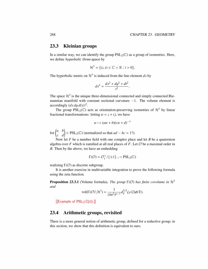
268 CHAPTER 23. GEOMETRY
23.3 Kleinian groups
In a similar way, we can identify the group PSL2(C) as a group of isometries. Here,we define hyperbolic three-space by
H3 = {(z, t) ∈ C× R : t > 0}.
The hyperbolic metric onH3 is induced from the line element ds by
ds2 =dx2 + dy2 + dt2
t2 .
The space H3 is the unique three-dimensional connected and simply connected Rie-mannian manifold with constant sectional curvature −1. The volume element isaccordingly (dx dy dt)/t3.
The group PSL2(C) acts as orientation-preserving isometries of H3 by linearfractional transformations: letting w = z + t j, we have
w 7→ (aw + b)(cw + d)−1
for(a bc d
)∈ PSL2(C) (normalized so that ad − bc = 1?).
Now let F be a number field with one complex place and let B be a quaternionalgebra over F which is ramified at all real places of F. Let O be a maximal order inB. Then by the above, we have an embedding
Γ(O) = O×1 /{±1} ↪→ PSL2(C)
realizing Γ(O) as discrete subgroup.It is another exercise in multivariable integration to prove the following formula
using the zeta function.
Proposition 23.3.1 (Volume formula). The group Γ(O) has finite covolume in H3
andvol(Γ(O)\H3) =
1(4π2)n−1 d3/2
F ζF(2)φ(D).
[[Example of PSL2(Z[i]).]]
23.4 Arithmetic groups, revisited
There is a more general notion of arithmetic group, defined for a reductive group; inthis section, we show that this definition is equivalent to ours.

23.5. ORTHOGONAL GROUP 269
23.5 Orthogonal group
Rephrase in terms of orthogonal group, with an eye toward generalizations.[[I’m pretty sure that this implies that an automorphism of a quaternion algebra
has to be inner, giving a quadratic forms proof of Skolem–Noether.]]
23.6 Extensions and further reading
Exercises
In these exercises, we maintain the notation in this section: let F be a number fieldwith ring of integers R, and let O be an R-order in a quaternion algebra B over F.
23.1. Show that R is discrete in FR = F ⊗Q R. [Hint: it is enough to show this fora neighborhood of 0, and then use the fact that the norm must be an integer.]Use this to show that O is discrete in B⊗Q R.
23.2. Let d ∈ R \ Q. Show that Z[√
2] is not discrete in R. (This gives a reason toworry about discreteness of number fields when we project.)
23.3. Show that the image ofO×1 in a projection to any proper factor of SL2(R)r−d×SL2(C)c is not discrete.
23.4. Let B =
(a, bF
)be a quaternion algebra over a number field F ↪→ R. LetO ⊂ B
be an order. Show that O×1 is discrete in SL2(R) if and only if k is totally realand for all nonidentity real places v, we have v(a), v(b) < 0.
23.5. In this exercise, we give a direct argument for the discreteness of an arithmetic
Fuchsian group. Let B =
(a, bF
)be a quaternion algebra over a totally real
number field F ↪→ R. Let O ⊂ B be an order. Suppose that B is ramified atall nonidentity real places. We will show that O×1 is discrete in SL2(R).
a) Suppose not: then there exists a sequence αn = tn + xni + yn j + zni j→ 1with tn, xn, yn, zn ∈ F with bounded denominators. Multiplying through,assume that all coordinates are integral. Thus for n sufficiently large, allof the coordinates are integral and bounded.
b) Show that for all nonidentity v, the coordinates of v(αn) are also boundedusing compactness.

270 CHAPTER 23. GEOMETRY
c) Show that there are only a finite number of elements in R that are boundedin each coordinate (all conjugates are bounded); look at the coefficientsof a minimal polynomial. Derive a contradiction.
23.6. If H ↪→ G1,G2 is a subgroup of topological groups G1 and G2, H ↪→ G1×G2is discrete, and G1 is compact, then H ↪→ G2 is discrete.

Chapter 24
Fuchsian and Kleinian groups:examples
24.1 Triangle groups
271


Chapter 25
Embedding numbers
25.1 Representation numbers
Of binary quadratic forms by indefinite quaternary forms or integers by indefiniteternary quadratic forms.
25.2 Selectivity
25.3 Isospectral, nonisometric orbifolds
Sunada and Vigneras.
25.4 Extensions and further reading
Exercises
25.1.
273

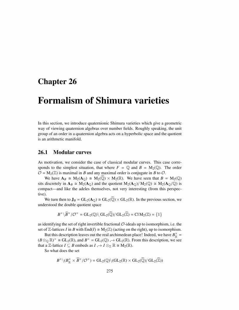
Chapter 26
Formalism of Shimura varieties
In this section, we introduce quaternionic Shimura varieties which give a geometricway of viewing quaternion algebras over number fields. Roughly speaking, the unitgroup of an order in a quaternion algebra acts on a hyperbolic space and the quotientis an arithmetic manifold.
26.1 Modular curves
As motivation, we consider the case of classical modular curves. This case corre-sponds to the simplest situation, that where F = Q and B = M2(Q). The orderO = M2(Z) is maximal in B and any maximal order is conjugate in B to O.
We have AB � M2(AQ) � M2(Q) × M2(R). We have seen that B = M2(Q)sits discretely in AB � M2(AQ) and the quotient M2(AQ)/M2(Q) � M2(AQ/Q) iscompact—and like the adeles themselves, not very interesting (from this perspec-tive).
We turn then to JB = GL2(AQ) � GL2(Q)×GL2(R). In the previous section, weunderstood the double quotient space
B×\B×/O× = GL2(Q)\GL2(Q)/GL2(Z) = Cl M2(Z) = {1}
as identifying the set of right invertible fractionalO-ideals up to isomorphism, i.e. theset of Z-lattices I in B with End(I) � M2(Z) (acting on the right), up to isomorphism.
But this description leaves out the real archimedean place! Indeed, we have B×R =
(B⊗Q R)× � GL2(R), and B× = GL2(Q) ↪→ GL2(R). From this description, we seethat a Z-lattice I ⊆ B embeds as I ↪→ I ⊗Z R � M2(R).
So what does the set
B×\(B×R × B×/O×) = GL2(Q)\(GL2(R)× GL2(Q)/GL2(Z))
275

276 CHAPTER 26. FORMALISM OF SHIMURA VARIETIES
represent? Here, note that O× acts by right multiplication on B× but B× acts by leftmultiplication (embedded diagonally) on both factors B×R × B×.
As it stands, this is not yet interesting: by the aboveOther orders include those defined by congruence conditions: for example, for
each N ∈ Z>0, we have
O0(N) =
{(a bc d
): N | c
}and
O(N) =
{(a bc d
): N | c,N | b, a ≡ d (mod N)
}.
To introduce the adelic description, we first give its derivation for the spaceY(1)C. We have seen that Y(1)C is in bijection with the set of lattices in C up toisomorphism, which we denote � \Lat(C). But in fact a lattice in C is really a lat-tice in R2 together with a complex structure ψ : C → EndR(R2), and these are
in bijection with C \ R = H± as follows: choose M =
(a bc d
)∈ M2(R) such that
M(
0 1−1 0
)M−1 = ψ(i); then we take τ =
ai + bci + d
∈ H±. Therefore Y(1)C is in
bijection with
� \(H± × Lat(R2)) = GL2(R)\(H± × Lat(R2)).
And for every lattice Λ ∈ Lat(R2), we can find an M ∈ GL2(R) such that MΛ ⊆Q2 ⊆ R2, so this set is also in bijection with GL2(Q)\(H± × Lat(Q2)).
Next, we introduce the adeles. For a Z-module S , we define S = S ⊗Z Z, whereZ = lim←−Z/nZ. We then see that the map
Lat(Q2)→ Lat(Q2)
Λ 7→ Λ
is a bijection, with inverse Λ 7→ Λ ∩ Q2. Now since GL2(Q) acts transitively onLat(Q2), with stabilizer of a lattice Λ given by GL2(Z), we have in sum a bijection
Y(1)(C)↔ GL2(Q)\(H± ×GL2(Q)/GL2(Z)).
This gives a description for the quaternion algebra B = M2(Q). For any indefinitequaternion algebra B over Q with maximal order O, we have in a similar way the set
B∗\(H± × B∗/O∗).

26.2. MODULAR FORMS 277
This description can be seen exactly as the set of (real) lattices inside B⊗QR togetherwith a complex structure, up to isomorphism.
One then proves that this set has the structure of a complex manifold, and wehave:
Theorem 26.1.1 (Deligne). There exists a curve XBQ defined over Q, and an analytic
isomorphismXBQ(C) ∼−→ B∗\(H± × B∗/O∗).
Remark 26.1.2. It is more natural to define a Shimura curve by giving an incoherentquaternion algebra.
26.2 Modular forms
26.3 Global embeddings
26.4 Extensions and further reading
Exercises


Chapter 27
Definite quaternion algebras
27.1 Class numbers
Class number 1
27.2 Two-sided ideals
Exercise from Kimberly.
27.3 Theta functions
Application to sums of squares, the level is the minimal integer N such that NQ−1 isintegral. For individual quadratic forms, get an explicit answer. For general quadraticforms, estimate the coefficients.
27.4 Brandt matrices
27.5 Jacquet-Langlands correspondence
[[Trace formula for GL2(F) in Ling’s book; Zagier]]. [[Hijikata, “Explicit for-mula”]].
27.6 Relationship to elliptic curves
In this section, we discuss the relationship between endomorphism rings of supersin-gular elliptic curves and quaternion algebras, with applications to modular forms.
279

280 CHAPTER 27. DEFINITE QUATERNION ALGEBRAS
Let E be an elliptic curve over field k. For each (nonzero) isogeny (finite surjec-tive homomorphism) f : E → E′, there exists a dual isogeny f∨ : E′ → E such thatf∨ ◦ f is equal to multiplication by the degree deg f ∈ Z>0. In particular, the dual ∨
on End(E) = Endk(E) yields a nonsingular standard involution on End(E).The Q-algebra End(E)Q = End(E) ⊗Z Q is a division ring, and therefore from
previous work, it follows that End(E)Q is either Q, an imaginary quadratic field K,or a quaternion algebra over Q.
In fact, the latter possibility can only occur when char k = p, and we say E issupersingular : equivalently,
(i) End(E)Q has rank 4 as a Q-algebra;
(ii) E[p](k) = 0;
(iii) Tr(φ) ≡ 0 (mod p) where φ is the Frobenius endomorphism.
If #k = p ≥ 5 then E is supersingular if and only if #E(k) = p + 1.Let E be a supersingular elliptic curve; then E may be defined over a finite field
k of characteristic p. We will start from (i) and show in fact that End(E) is a maximalorder in the quaternion algebra ramified at p and∞; this result is due to Deuring, butwe follow a proof given by Lenstra.
Let O = End E and B = O ⊗Z Q. Whenever n ∈ Z>0 is prime to p, there is anisomorphism
E[n] = E[n](k) � Z/nZ⊕ Z/nZ
as abelian groups, so the endomorphism ring of this abelian group is End E[n] �M2(Z/nZ). By the existence of the dual isogeny, E[n] is a faithful module overO/nO, i.e. the mapO/nO → End E[n] is injective. Since #O/nO = # End E[n], thismap is an isomorphism.
It follows that for every prime ` , p, the map
O ↪→ O` = O ⊗Z Z`∼−→ End E[`∞] = lim
nE[`n](k) = T`E � M2(Z`)
is an isomorphism, and in particular O` is maximal and B is split at `.Since B is a division ring, it follows that B is ramified at p at infinity.For f ∈ O, let degi f be the inseparable degree of f , which is a power of p.
We put degi 0 = ∞. Then we have degi( fg) = degi( f ) degi(g) and degi( f + g) ≥min{degi f , degi g}—this follows from the fact that degi f is divisible by a givenpower q of p if and only if f factors via the qth power Frobenius morphism E → E(q).It follows that degi : End(E)Q → Z ∪ {∞} is a valuation on End(E)Q. Extended toEnd(E)Qp , this valuation “agrees” with the usual valuation on Qp, since degi p = p2;factoring an isogeny into its separable and inseparable parts (the latter a power of

27.6. RELATIONSHIP TO ELLIPTIC CURVES 281
Frobenius) shows that degi f = ordp( f∨ ◦ f ). Hence Op is the valuation ring of Bp
and hence maximal. This shows that O itself is maximal in B.Consider the category SSEll of supersingular elliptic curves over k, an alge-
braically closed field of characteristic p. The objects of SSEll are supersingular ellip-tic curves over k and the morphisms are isogenies. Choose a base object E ∈ SSEll,and let O = End(E) and B = O ⊗Z Q as above. For any other E′ ∈ SSEll, theHomk(E, E′) = Hom(E, E′) has the structure of a right O-module (precomposing)and the structure of a left O′ = End(E′)-module (postcomposing).
Let J be a (nonzero) integral left O-ideal. Define
E[J] = E[J](k) = {P ∈ E(k) : f (P) = O for all f ∈ I}.
Then E[J] is a finite subgroup of E and every finite subgroup of E is of the form E[J]for some left O-ideal J. (In fact, #E[J] = nrd(J).)
Let E′ = E/E[J] and consider the quotient map φ : E → E′ and its dualφ∨ : E′ → E. Then post-composing with φ∨ gives an injective map Hom(E, E′) →End(E) = O.
Let O′ = End(E′). Then we have an embedding O′ ↪→ O of Z-modules byg 7→ φ
∨gφ, and an element f ∈ O gives rise to such an endomorphism if and only if
f (E[J]) ⊂ E[J] if and only if (J f )(E[J]) = {O} if and only if J f ⊂ J if and only iff ∈ OR(J). In this way, we identify End(E′) � OR(J).
If E′ ∈ SSEll then End(E′) is isomorphic to a maximal order in B so End(E′) �OR(J) for some left O-ideal J; considering the dual isogeny, we see that End(E′) �OL(I) for the right O-ideal I = J−1.
In this correspondence, we identify Hom(E′, E) = J since s ∈ O factors via E′
if and only if s ∈ J. Dualizing, we have Hom(E, E′) = I. In particular, this impliesthat Hom(E1, E2) � I2I−1
1 � (I2 : I1)L and so
Hom(E1, E2)→ Hom(I1, I2)
f 7→ (φ 7→ f ◦ φ)
is bijective.Let ModO be the category of rightO-modules with morphisms given by nonzero
(right O-module) homomorphisms. We have proven the following proposition.
Proposition 27.6.1 (Kohel [Koh96, Theorem 45]). The association
Hom(E,−) : SSEll→ ModO
is a functor and defines an equivalence of categories.
Proof. We have shown that Hom(E,−) is full, faithful, and essentially surjective.
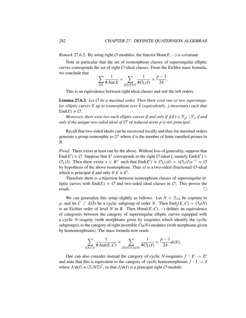
282 CHAPTER 27. DEFINITE QUATERNION ALGEBRAS
Remark 27.6.2. By using right O-modules, the functor Hom(E,−) is covariant.
Note in particular that the set of isomorphism classes of supersingular ellipticcurves corresponds the set of right O-ideal classes. From the Eichler mass formula,we conclude that ∑
[E]
1# Aut E
=∑
[I]∈ClO
1#OL(I)
=p− 1
24.
This is an equivalence between right ideal classes and not the left orders.
Lemma 27.6.3. Let O be a maximal order. Then there exist one or two supersingu-lar elliptic curves E up to isomorphism over k (equivalently, j-invariants) such thatEnd(E) � O.
Moreover, there exist two such elliptic curves if and only if j(E) ∈ Fp2 \Fp if andonly if the unique two-sided ideal of O′ of reduced norm p is not principal.
Recall that two-sided ideals can be recovered locally and thus for maximal ordersgenerate a group isomorphic to Zd where d is the number of finite ramified primes inB.
Proof. There exists at least one by the above. Without loss of generality, suppose thatEnd(E′) � O. Suppose that E′ corresponds to the right O-ideal I, namely End(E′) =
OL(I). Then there exists x ∈ B× such that End(E′) � OL(xI) = xOL(I)x−1 = Oby hypothesis of the above isomorphism. Thus xI is a two-sided (fractional) O-idealwhich is principal if and only if E � E′.
Therefore there is a bijection between isomorphism classes of supersingular el-liptic curves with End(E) � O and two-sided ideal classes in O. This proves theresult.
We can generalize this setup slightly as follows. Let N ∈ Z>0 be coprime top, and let C ⊂ E(k) be a cyclic subgroup of order N. Then Endk(E,C) = O0(N)is an Eichler order of level N in B. Then Hom((E,C),−) defines an equivalenceof categories between the category of supersingular elliptic curves equipped witha cyclic N-isogeny (with morphisms given by isogenies which identify the cyclicsubgroups), to the category of right invertibleO0(N)-modules (with morphisms givenby homomorphisms). The mass formula now reads∑
[(E,C)]
1# Aut(E,C)
=∑
[I]∈ClO0(N)
1#OL(I)
=p− 1
24ψ(N).
One can also consider instead the category of cyclic N-isogenies f : E → E′
and note that this is equivalent to the category of cyclic homomorphisms f : I → Jwhere J/φ(I) � (Z/NZ)2, so that J/φ(I) is a principal right O-module.

27.6. RELATIONSHIP TO ELLIPTIC CURVES 283
Example 27.6.4. Consider p = 11. The algebra B =
(−1,−11Q
)has discriminant 11
and the maximal order O generated by i and (1 + j)/2. We have # ClO = 2, with thenontrivial class represented by the ideal I generated by 2 and 1 + i(1 + j)/2.
We have O× = 〈i〉 of order 4 and OL(I) = 〈1/2 − i(1 + j)/4〉 of order 6, andindeed 1/4 + 1/6 = 10/24 = 5/12. The two supersingular curves modulo 11 are theones with j-invariants 0 and 1728 ≡ 1 (mod 11), and End(E) � O if j(E) = 1728whereas for End(E′) � O′ we have Hom(E, E′) � I, in other words, E′ � E/E[I].
Let I1, . . . , Ih be representatives for the set ClO. Let Oi = OL(Ii) and let wi =
#O×i . The products Mi j = I jI−1i are fractionalOi,O j-ideals. If Ei is an elliptic curve
with End(Ei) = Oi, then we have Ii = Hom(E, Ei) hence Mi j = I jI−1i = Hom(Ei, E j).
Define the theta series θi j(q) by
θi j(q) =1w j
∑x∈Mi j
exp(2πi nrd(x)/ nrd(Mi j)τ) =∑m≥0
Bi j(m)qm
where q = exp(2πiτ).The functions θi j as functions on the upper half-plane (for τ ∈ H) are modular
forms of weight 2 for the group Γ0(p). Their Fourier coefficients Bi j(m) give theentries of the Brandt matrix B(m) = (Bi j(m))i, j=1,...,h. We have B(1) is the identitymatrix.
Example 27.6.5. We return to the example p = 11.Let I1 = O and I2 = I. We have M11 = O, and in the basis 1, i, (1+ j)/2, i(1+ j)/2
we have nrd(x, y, z, w) = x2 + xz + y2 + yw + 3w2 + 3z2, so
θ11(q) =14
(1 + 4q + 4q2 + 8q3 + 20q4 + 16q5 + 32q6 + . . . ).
In a similar way, we have the basis 2, 2i, 1− 3/2i− 1/2i j, 3/2− i− 1/2 j for I and
θ12(q) =16
(1 + 12q2 + 12q3 + 12q4 + 12q5 + . . . )
and θ21(q) = 32θ12(q) and
θ22(q) =16
(1 + 6q + 6q3 + 24q4 + 18q5 + 32q6 + . . . ).
Indeed, B(1) is the identity matrix.
Example 27.6.6. In the case p = 11, we have B(2) =
(1 23 0
)with characteristic
polynomial (T − 3)(T + 2). The eigenvalue 3 = 2 + 1 corresponds to an Eisenstein

284 CHAPTER 27. DEFINITE QUATERNION ALGEBRAS
series, and the eigenvalue −2 corresponds to the (isogeny class of the) elliptic curveX0(11) given by the equation y2 + y = x3 − x2 − 10x − 20: indeed, #X0(11)(F2) =
2 + 1− (−2) = 5.
Lemma 27.6.7. The entry Bi j(m) is equal to the number of subgroups C of order min Ei such that Ei/C = E j.
Return to example with maximal unit group (icosahedron group) and mass for-mula.
27.7 Ramanujan graphs
Let G be a k-regular connected graph with n vertices and with adjacency matrix Tand combinatorial Laplacian k − T whose eigenvalues are 0 < µ− 1 ≤ µ2 ≤ · · · ≤µn−1 ≤ 2k. (Adjusted average a function on the neigbors of v.) The expansioncoefficient of G is
h(G) = min#S≤n/2
#∂S#S
.
One is interested in getting a large coefficient.Tanner, Alon-Milman:
2µ1
k + 2µ1≤ h(G) ≤
√2kµ1
Alon-Boppana:lim inf λ2(G) ≥ 2
√k − 1.
Define Ramanujan graph, random graph is Ramanujan.A k-regular infinite tree is the ideal expander, with expansion coefficient k − 1.
Find subgroups of its automorphism group that does not identify vertices that are tooclose to each other. Bruhat-Tits tree, identify units of norm 1.
Bound on the eigenvalues of the adjacency matrix is given by the Ramanujan-Petersson bound on coefficients.
27.8 Extensions and further reading
Exercises
27.1. Consider the analogous isogeny tree of CM elliptic curves.

Chapter 28
Drinfeld modules and functionfields
In this chapter, we discuss the function field side of the global field picture.
28.1 Extensions and further reading
Exercises
285


Part IV
Concluding material
287


Chapter 29
Other topics
29.1 Quaternionic polynomial rings
29.2 Matrix rings over quaternion rings
29.3 Unitary groups and Hermitian forms
29.4 Unit groups of integral group rings
In Z[G] for G a finite group, get interesting unit groups.
29.5 Representation theory of quaternion algebras
29.6 Quaternion rings and Azumaya algebras
Neukirch, get references from my paper, including GL and Lucianovic.
29.7 Octonions and composition algebras
29.8 Lie theory
289

Appendix A
Hints and solutions to selectedexercises
1.1 If B contains C, then B is a C-vector space, so B has even dimension as an R-vector space. Or see May [May66, p. 290]: if i j = a + bi + c j with a, b, c ∈ R,multiply on the left by i, and derive a contradiction.
2.3 For such a map, we must have i j 7→(
0 1−1 0
). Check that the four matrices
are linearly independent, so the map is an F-linear isomorphism. Then, us-ing the universal property of algebras given by generators and relations, showthat the given matrices satisfy the relations in B, so the map is an F-algebrahomomorphism.
2.7 Use Exercise 2.4(c) and show that the center over F has dimension 1 or com-pute directly with xi− ix = x j− jx = 0 for x = u + vi + w j + zk ∈ B.
2.13 Use the left regular representation either to F or a subfield K, and use the blockmatrix determinant. See also Aslaksen [Asl96].
3.3 It is (x, y) 7→ (y, x). Note that F embeds diagonally in F × F.
3.5 g 7→ g−1 is a standard involution if and only if G has exponent 2 and char F = 2(so the standard involution is the identity and F[G] is commutative).
3.8 Let i, j ∈ K \ F. Then i + j satisfies a quadratic polynomial, but ji = i j, so wehave (i+ j)2 = i2 +2i j+ j2 ∈ F(i+ j)+ F hence 2i j = c(i+ j)+d with c, d ∈ F:but then since 2 , 0, we have 2i , c ∈ F so j = (ci + d)/(2i− c) ∈ K.
291
292 APPENDIX A. HINTS AND SOLUTIONS TO SELECTED EXERCISES
3.9 For part (a), Suppose B has degree 2. Choose a basis 1, x2, . . . , xm. For eachi, the quadratic F-algebras F[xi] have a standard involution, and so extendingby F-linearity we obtain a map : B → B. For x ∈ B, let t(x) = x + x andn(x) = xx.
By induction and F-linearity, we may suppose 1, x, y are F-linearly indepen-dent. Suppose (x + y)2 − s(x + y) + m = 0 with s,m ∈ F. We show thats = t(x) + t(y). We have
(x− y)2 = x2 − (xy + yx) + y2 = 2(x2 + y2)− s(x + y) + m
= (2t(x)− s)x + (2t(y)− s)y + (m− 2n(x)− 2n(y))
But (x − y)2 ∈ F(x − y) + F so 2t(x) − s = s − 2t(y), i.e. 2s = 2t(x) + 2t(y).Since char F , 2, we have s = t(x) + t(y) as desired.
To conclude, we show xy = y x. We may suppose xy < F. We verify that both(xy)2 − (xy + y x)xy + (y x)(xy) = 0 and (xy)2 − (xy + xy)xy + xy(xy) = 0, sothe result follows by uniqueness of the minimal polynomial.
For part (b), by the uniqueness of the standard involution, we have x = x + 1if x < F. But then if 1, x, y are F-linearly independent we have x + y + 1 =
x + y = x + y = (x + 1) + (y + 1) = x + y, a contradiction. So dimF2 B ≤ 2.Since a Boolean ring consists of idempotents, we have B = F2 or B � F2
2.
3.10 Under right multiplication by B = Mn(F), a matrix is nothing other than thedirect sum of its rows, so in particular, the characteristic polynomial of rightmultiplication by A ∈ Mn(F) acting on Mn(F) will be the nth power of theusual characteristic polynomial of A acting on row vectors V � Fn. (In thelanguage of Chapter 6, B = Mn(F) as a right B-module is B � Vn whereV � Fn is the unique simple right B-module.)
3.11 By F-linearity, it suffices to verify these statements on a basis for B.
3.14 See van Praag [vPr68] (or its summary [vPr02, Remark 4]).
4.5 For part (a), to simplify the proof of the second statement, choose a normalizedbasis for V .
4.7 For part (c), by the transitivity of trace, we may assume K/F is purely insepara-ble and [K : F] is a multiple of p. But then all roots of the minimal polynomialof x ∈ K over F are equal, so the characteristic polynomial of multiplicationby x ∈ K has all roots equal and there are a multiple of p of them and thus thetrace is zero.

293
For part (d), Tr((a + b√
5)2) = 2(a2 + 5b2) and
Tr((a + bα + cα2)2) = 2(a2 − 2ab + 10ac + 5b2 − 8bc + 13c2).
4.9 If B =
(a, bFq
)then K = Fq(i) � Fq2 and N : Fq2 → Fq is surjective so
b ∈ NK/F(K×).
4.10 If i, j and i′, j′ are generators, respectively, then consider the subalgebras gen-erated by i⊗ 1 and j⊗ j′, and i⊗ i′ and 1⊗ j′.
4.13 For the first, exhibit an explicit isometry 〈1, 1, 1〉 � 〈2, 3, 6〉. For the second,note that 〈2, 5, 10〉 represents 7 but 〈1, 1, 1〉 does not (by showing x2 +y2 + z2 +
w2 . 0 (mod 8) for x, y, z, w ∈ Z with gcd(x, y, z, w) = 1); or note that 〈1, 1, 1〉represents 1 but 〈2, 5, 10〉 (looking modulo 5, and arguing similarly).
5.2 Choose 0 , y ∈ K⊥.
14.10 See Shimura [Shi71, Proposition 4.11, (5.4.2)].
6.2 The map a ⊗ b 7→ (x 7→ axb) gives an F-algebra homomorphism B⊗F B →EndF(B) � M4(F), which is injective since B⊗F B is simple and therefore anisomorphism by a dimension count.
6.6 The augmentation ideal is the kernel of the surjective map∑g agg 7→
∑g ag,
so is nontrivial.
6.12 This exercise was given in a course by Bjorn Poonen in Spring 2000 at theUniversity of California, Berkeley.
First, parts (a) and (b). Choose x ∈ D \ F. Then K = F(x) is a purelyinseparable extension of F so the minimal polynomial of x in D (or in F) is ofthe form T pn − a. In particular, p | [K : F], but D is a left K-vector space and[D : F] = [D : K][K : F] so p | [D : F].
For part (c), all roots of the minimal polynomial of x are equal, hence alleigenvalues of x ⊗ 1 ∈ Mn(F) are equal, and the number of them is divisibleby p by (a), so the trace is zero. For part (d), by (c), all elements of Mn(F)have trace zero, which is a contradiction.
6.13 Let j ∈ B× satisfy jx j−1 = x. Then B = K ⊕ K j, but j2x j−2 = x so j2 ∈ Z(B)so j2 = b ∈ F×.

294 APPENDIX A. HINTS AND SOLUTIONS TO SELECTED EXERCISES
6.16 By Corollary 6.6.8, every maximal subfield K of B has the same dimension, sosince F is a finite field they are isomorphic (as abstract fields). But then by theSkolem–Noether theorem, since every element lies in a maximal subfield, wehave B× =
⋃x∈B× x−1K×x, which is a contradiction.
One can also proceed without using the maximal subfield dimension theorem.Suppose B is a minimal counterexample (by cardinality); then B is a divisionring, but every subalgebra of B is a field. Let F = Z(B). Let i ∈ B \ F; thenby minimality, the centralizer of i is a maximal subfield K. We may assumeK = F(i). If B = K, we are done. Otherwise, let i have multiplicative order m.Consider L : B→ B by L(x) = ixi−1. Then L is a K-linear map with Lm equalto the identity. We may therefore decompose B into eigenspaces for L. Arguingas in the case of quaternion division rings, we show that each such nonzeroeigenspace has dimension 1 as K-vector space. Now consider the normalizerN = NB(K). Then there is a bijection between the set of cosets of N/K× andthe eigenspaces of L. But N acts on K as F-linear automorphisms with kernelK×, so N/K× is a subgroup of the Galois group Gal(K/F). It must be thefull Galois group, otherwise N/K× fixes some subfield and its centralizer is anoncommutative F-subalgebra, contradicting minimality. Therefore dimK B =
dimF K. We now proceed as above.
8.6 Using the matrix units, show that if M = (mi j)i, j ∈ O then mi j · 1 ∈ O, butthen mi j is integral over R so in fact mi j ∈ R and hence M ∈ Mn(R).
8.8 The converse is true if char F , 2 and R is integrally closed. It is immediateif 1/2 ∈ R since trd(x2) = trd(x)2 − 2 nrd(x), so 2 nrd(x) ∈ R. But for thesame reason more generally we have 2 nrd(xn) = 2 nrd(x)n ∈ R so R[nrd(x)] ⊆(1/2)R; so if R is integrally closed we have in fact nrd(x) ∈ R.
The statement is false if char F = 2: take B = F × F (with char F = 2) andx = (a, a) with a ∈ F not integral over R. Then trd(xn) = 2an = 0 for all n butx is not integral.
10.2 The quadratic form 〈−1, e,−1〉 is isotropic by a previous exercise, so diag-onalizing we have 〈−1, e〉 � 〈1, s〉 for some s ∈ k×. But disc(〈−1, e〉) =
−e = s = disc(〈1, s〉) ∈ k×/k×2, so 〈1, s〉 � 1,−e〉. More generally, thisargument shows that two nonsingular binary quadratic forms over a finite fieldare isometric if and only if they have the same discriminant.
10.6 The proof that addition and multiplication are continuous with respect to theabsolute value | | induced by w is identical to the commutative case. We havea filtration O ⊃ P ⊃ P2 ⊃ . . . where P is generated by j and thus to show

295
that B is complete it suffices to note that the limit of the partial sums x0 + x1 j +
x2 j2 + · · · = (x0 + x2π + . . . ) + (x1 + x3π + . . . ) j ∈ K + K j exists since Kis complete. The set O is compact since it is complete and totally bounded.By translating, since O is open we have that B is locally compact. Finally, ifx < O then w(x) < 0 so the ring generated by O and x is equal to B; but B isnot compact, since the open cover
⋃i π−iO has no subcover.
10.13 Write B in the form B =
(K, 2Q2
)with K/Q2 the unique unramified extension of
Q2.
12.2 The lattices are free, so by induction we reduce to the one-dimensional case,which is simply the statement that Rp ∩ F = Rp ⊆ Fp and follows sinceRp = {x ∈ F : v(x) ≥ 0}.
11.5 Take t = ±q∏
p∈Σ\{∞} pordp(tp). Select the prime q to satisfy congruences toensure that the conditions hold. See [[Cassels, Corollary to Theorem 6.5.1]]
14.2 There exists nonzero r ∈ I = Ox so 1 = (y/r)x for some y ∈ O and hencex ∈ B×.
14.4 Reduce to the local case; the result follows from Paragraph 14.5.7. Considerthe connecting ideal I = OO′: clearly O ⊆ OL(I) so equality holds since O ismaximal. [[Or use hereditary?]]
14.12 This exercise is due to Kaplansky [Kap69]. We compute that
OL(I) =
R R (a)(a) R (a2)R R R
and OR(I) =
R R RR R R
(a2) (a2) R
and
I−1 =
R R RR R R
(a) R (a2)
has I−1I = OR(I) but
II−1 =
(a) R (a)(a) R (a2)R R R
, OL(I).
21.1 First compute all elements in O of norm 2, then show the product of any twoof these elements belongs to 2O.


Appendix B
Orders of small class number
Etc.
297

Bibliography
[Alb72] A. A. Albert, Tensor products of quaternion algebras, Proc. Amer.Math. Soc. 35 (1972), no. 1, 65–66.
[Alt89] Simon L. Altmann, Hamilton, Rodrigues, and the quaternion scandal,Math. Magazine 62 (1989), no. 5, 291–308.
[AO05] Simon L. Altmann and Eduardo L. Ortiz, eds., Mathematics and so-cial utopias in France: Olinde Rodrigues and his times, Amer. Math.Society, Providence, RI, 2005.
[Art26] Emil Artin, Zur Theorie der hyperkomplexen Zahlen, Abh. Math. Sem.Hamburgischen Univ. 5 (1926), 251-260.
[Art50] Emil Artin, The influence of J. H. M. Wedderburn on the developmentof modern algebra, Bull. Amer. Math. Soc. 56 (1950), no. 1, 65–72.
[Asl96] Helmer Aslaksen, Quaternionic determinants, Math. Intelligencer 18(1996), no. 3, Summer 1996, 57–65.
[Bae02] John C. Baez, The octonions, Bull. Amer. Math. Soc. (N.S.) 39 (2002),145–205; Errata for “The octonions”, Bull. Amer. Math. Soc. (N.S.)42 (2005), 213.
[BM58] R. Bott and J. Milnor, On the parallelizability of the spheres, Bull.Amer. Math. Soc. 64 (1958), 87–89.
[Bre10] Matej Bresar, An elementary approach to Wedderburn’s structure the-ory, Exposition. Math. 28 (2010), 79–83.
[Bro61] Bancroft H. Brown, Mathematics at Dartmouth: 1769–1961, Dedica-tory Conference, Albert Bradley Center for Mathematics, DartmouthCollege, Hanover, November 3, 1961.
299

300 BIBLIOGRAPHY
[Brz95] Juliusz Brzezinski, Definite quaternion orders of class number one, J.Theorie Nombres Bordeaux 7 (1995), 93–96.
[Brz83] Julius Brzezinski, On orders in quaternion algebras, Comm. Algebra11 (1983), no. 5, 501-522.
[Cay1845] Arthur Cayley, On Jacobi’s elliptic functions, in reply to the Rev. B.Bronwin; and on quaternions, Phil. Mag. 26 (1845), 208–211.
[Cli1878] William K. Clifford, Applications of Grassmann’s extensive algebra,Amer. Jour. Math. 1 (1878), 350–358.
[CS03] John H. Conway and Derek A. Smith, On quaternions and octonions:their geometry, arithmetic, and symmetry, A. K. Peters, Ltd., Natick,MA, 2003.
[Cox89] David A. Cox, Primes of the form x2 + ny2: Fermat, class field theory,and complex multiplication, John Wiley & Sons, Inc., New York, 1989.
[Cro64] Michael J. Crowe, A history of vector analysis, Mineola, NY, DoverPress, 1964.
[Dic03] Leonard Eugene Dickson, Definitions of a linear associative algebraby independent postulates, Trans. Amer. Math. Soc. 4 (1903), no. 1,21–26.
[Dic12] Leonard Eugene Dickson, Linear algebras, Trans. Amer. Math. Soc.13 (1912), no. 1, 59–73.
[Dic14] Leonard Eugene Dickson, Linear associative algebras and abelianequations, Trans. Amer. Math. Soc. 15 (1914), 31–46.
[Dic19] L. E. Dickson, On quaternions and their generalization and the historyof the eight square theorem, Ann. Math. (2) 20 (1919), no. 3, 155–171.
[Dic23] L. E. Dickson, Algebras and their arithmetics, Univ. of Chicago Press,Chicago, 1923.
[Die48] Jean Dieudonne, Sur les groupes classiques, Actualities scientifique etindustrielles, no. 1040, Paris, Hermann, 1948.
[Die53] Jean Dieudonne, On the structure of unitary groups (II), Amer. J. Math.75 (1953), 665–678.

BIBLIOGRAPHY 301
[DK95] Adel Diek and R. Kantowski, Some Clifford algebra history, CliffordAlgebras and Spinor Structures, Math. Appl. 321 (1995), 3–12.
[Eic53] Martin Eichler, Quadratische Formen und orthogonale Gruppen,Grundlehren Math. Wiss., vol. 63, Springer, New York, 1974.
[FD93] Benson Farb and R. Keith Dennis, Noncommutative algebra, Grad.Texts in Math., vol. 144, Springer-Verlag, New York, 1993.
[FS07] Della D. Fenster and Joachim Schwermer, Beyond class field theory:Helmut Hasse’s arithmetic in the theory of algebras in 1931, Arch.Hist. Exact Sci. 61 (2007), 425–456.
[Fro1878] F.G. Frobenius, Uber lineare Substitutionen und bilineare Formen, J.Reine Angew. Math. 84 (1878), 1–63.
[vzGG03] Joachim von zur Gathen and Jurgen Gerhard, Modern computer alge-bra, 2nd edition, Cambridge University Press, Cambridge, 2003.
[Gau00] Carl Friedrich Gauss, Mutation des Raumes, in Carl Friedrich GaussWerke, Band 8, Konig. Gesell. Wissen., Gottingen, 1900, 357–361.
[Gras1862] Hermann Grassmann, Die Ausdehnungslehre. Vollstaandig und instrenger Form begrundet [Extension theory], Berlin, Wiegand, 1862.
[Grav1882] Robert Perceval Graves, Life of Sir William Rowan Hamilton, VolumeI, Dublin University Press, 1882.
[Grav1885] Robert Perceval Graves, Life of Sir William Rowan Hamilton, VolumeII, Dublin University Press, 1885.
[Grav1889] Robert Perceval Graves, Life of Sir William Rowan Hamilton, VolumeIII, Dublin University Press, 1889.
[GL09] Benedict H. Gross and Mark W. Lucianovic, On cubic rings andquaternion rings, J. Number Theory 129 (2009), no. 6, 1468-1478.
[Ham1843] William R. Hamilton, On a new species of imaginary quantities con-nected with a theory of quaternions, Proc. Royal Irish Acad. 2 (1843),424–434.
[Ham1844] William R. Hamilton, On quaternions, or on a new system of imaginar-ies in algebra: copy of a letter from Sir William R. Hamilton to JohnT. Graves, Esq. on quaternions, Philosophical Magazine 25 (1844),489–495.
302 BIBLIOGRAPHY
[Ham1853] W. R. Hamilton, Lectures on quaternions, Cambridge, Cambridge Uni-versity Press, 1853.
[Ham1866] W. R. Hamilton, Elements of quaternions, Cambridge, CambridgeUniversity Press, 1866.
[Ham1899] Hamilton’s quaternions, review of Elements of quaternions, Nature,August 24, 1899, 387.
[Ham67] W. R. Hamilton, The mathematical papers of Sir William RowanHamilton, Vol. III: Algebra, eds. H. Halberstam and R. E. Ingram,Cambridge University Press, 1967.
[Han80] Thomas L. Hankins, William Rowan Hamilton, Johns Hopkins Univer-sity Press, 1980.
[Han06] Andrew J. Hanson, Visualizing quaternions, Morgan Kaufmann, SanFrancisco, 2006.
[Hap80] Dieter Happel, Klassifikationstheorie endlich-dimensionaler Algebrenin der Zeit von 1880 bis 1920, Enseign. Math. (2) 26 (1980), no. 1–2,91-102.
[Har1881] A. S. Hardy, Elements of quaternions, Ginn, Heath, and Company,Boston, 1881.
[HFK94] John C. Hart, George K. Francis, Louis H. Kauffman, Visualizingquaternion rotation, ACM Trans. Graphics 13 (1994), no. 3, 256–276.
[Haw00] Thomas Hawkins, The emergence of the theory of Lie groups: an essayin the history of mathematics, 1869–1926, Springer, New York, 2000.
[Hur1888] Adolf Hurwitz, Uber die Komposition der quadratischen Formen vonbeliebig vielen Variablen, Nach. der kobig. Gesell. Wissen. Gottingen,Math.-Physik. Klasse, 1898, 309–316.
[Jah10] Majid Jahangiri, Generators of arithmetic quaternion groups and aDiophantine problem, Int. J. Number Theory 6 (2010), no. 6, 1311–1328.
[Kap69] Irving Kaplansky, Submodules of quaternion algebras, Proc. LondonMath. Soc. (3) 19 (1969), 219–232

BIBLIOGRAPHY 303
[Kar10] Max Karoubi, K-theory, an elementary introduction, Cohomology ofgroups and algebraic K-theory, Adv. Lect. Math. (ALM), vol. 12, Int.Press, Somerville, MA, 2010, 197-215.
[Ker58] M. Kervaire, Non-parallelizability of the n-sphere for n > 7, Proc. Nat.Acad. Sci. 44 (1958) 280-283.
[Kil1888] Wilhelm Killing, Die Zusammensetzung der stetigen endlichen Trans-formations-gruppen, Math. Ann. 31 (1888), 252–290; Math. Ann. 33(1888), 1–48; Math. Ann. 34 (1889), 57–122; Math. Ann. 36 (1890),no. 2, 161–189.
[Koh96] David Kohel, Endomorphism rings of elliptic curves over finite fields,Ph.D. thesis, University of California, Berkeley, 1996.
[Lam01] Tsit-Yuen Lam, A first course in noncommutative rings, 2nd. ed., Grad-uate texts in math., vol. 131, Springer-Verlag, New York, 2001.
[Lam02] Tsit-Yuen Lam, On the linkage of quaternion algebras, Bull. Belg.Math. Soc. 9 (2002), 415–418.
[Lam03] Tsit-Yuen Lam, Hamilton’s quaternions, Handbook of algebra, vol. 3,North Holland, Amsterdam, 2003, 429–454.
[Lam05] Tsit-Yuen Lam, Introduction to quadratic forms over fields, Graduatestudies in math., vol. 67, American Mathematical Society, Providence,2005.
[Lan67] C. Lanczos, William Rowan Hamilton—An appreciation, Amer. Sci-entist 55 (1967), 129–143.
[Lem11] Stefan Lemurell, Quaternion orders and ternary quadratic forms,2011, arXiv:1103.4922.
[Lev13] Alex Levin, On the classification of algebras, M.Sc. thesis, Universityof Vermont, 2013.
[Lew06] David W. Lewis, Quaternion algebras and the algebraic legacy ofHamilton’s quaternions, Irish Math. Soc. Bull. 57 (2006), 41–64.
[MR03] Colin Maclachlan and Alan W. Reid, The arithmetic of hyperbolic 3-manifolds, Grad. Texts in Math., vol. 219, Springer-Verlag, New York,2003.

304 BIBLIOGRAPHY
[Mat69] Hideya Matsumoto, Sur les sous-groupes arithmetiques des groupessemi-simples deployes, Ann. Sci. Ecole Norm. Sup. (4) 2 (1969), 1-62.
[Max1869] J. C. Maxwell, Remarks on the mathematical classification of physicalquantities, Proc. London Math. Soc. 3 (1869), 224–232.
[May66] Kenneth O. May, The impossibility of a division algebra of vectors inthree dimensional space, Amer. Math. Monthly 73 (1966), no. 3, 289–291.
[Mil] J.S. Milne, Class field theory,http://www.jmilne.org/math/CourseNotes/cft.html.
[1] Eliakim Hastings Moore, General analysis, Part I, Memoirs Amer.Phil. Soc., vol. 1, Amer. Phil. Soc., Philadelphia, 1935.
[Neu99] Jurgen Neukirch, Algebraic number theory, Grundlehren Math. Wiss.,vol. 322, Springer-Verlag, Berlin, 1999.
[OCa00] Fiacre O Cairbre, William Rowan Hamilton (1805–1865), Ireland’sgreatest mathematician, Rıocht na Midhe (Meath Archaeological andHistorical Society) 11 (2000), 124–150.
[OCa10] Fiacre O Cairbre, Twenty years of the Hamilton walk, Irish Math. Soc.Bulletin 65 (201), 33–49.
[O’Do83] Sean O’Donnell, William Rowan Hamilton, Boole Press Limited,1983.
[Pei1882] Benjamin Peirce, Linear associative algebra, Amer. J. Math. 4 (1881),no. 1–4, 97-229.
[Pie82] Richard S. Pierce, Associative algebras, Springer–Verlag, New York,1982.
[Puj12] Jose Pujol, Hamilton, Rodrigues, Gauss, quaternions, and rotations: ahistorical reassessment, Comm. Math. Anal. 13 (2012), no. 2, 1–14.
[Rei03] Irving Reiner, Maximal orders, London Math. Soc. Monogr. (N.S.),vol. 28, Clarendon Press, Oxford University Press, Oxford, 2003.
[Rod1840] Olinde Rodrigues, Des lois geometriques qui regissent les deplace-ments d’un systeme solide dans l’espace, et la variation des coor-donnees provenant de ses deplacements consideres independamment
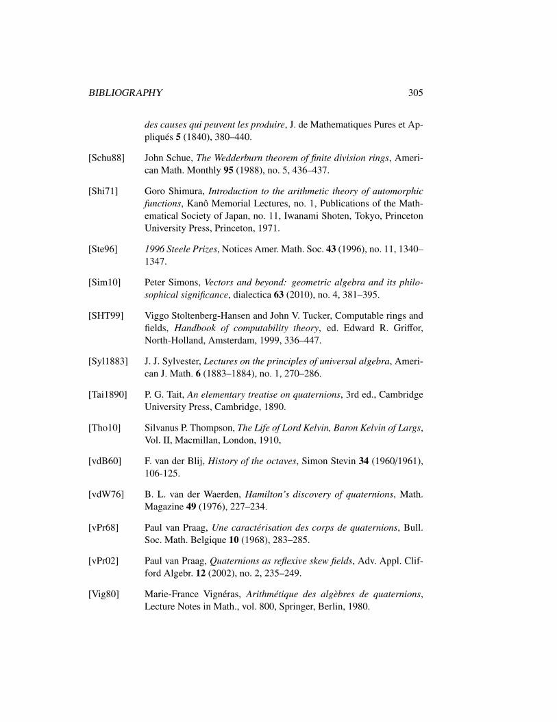
BIBLIOGRAPHY 305
des causes qui peuvent les produire, J. de Mathematiques Pures et Ap-pliques 5 (1840), 380–440.
[Schu88] John Schue, The Wedderburn theorem of finite division rings, Ameri-can Math. Monthly 95 (1988), no. 5, 436–437.
[Shi71] Goro Shimura, Introduction to the arithmetic theory of automorphicfunctions, Kano Memorial Lectures, no. 1, Publications of the Math-ematical Society of Japan, no. 11, Iwanami Shoten, Tokyo, PrincetonUniversity Press, Princeton, 1971.
[Ste96] 1996 Steele Prizes, Notices Amer. Math. Soc. 43 (1996), no. 11, 1340–1347.
[Sim10] Peter Simons, Vectors and beyond: geometric algebra and its philo-sophical significance, dialectica 63 (2010), no. 4, 381–395.
[SHT99] Viggo Stoltenberg-Hansen and John V. Tucker, Computable rings andfields, Handbook of computability theory, ed. Edward R. Griffor,North-Holland, Amsterdam, 1999, 336–447.
[Syl1883] J. J. Sylvester, Lectures on the principles of universal algebra, Ameri-can J. Math. 6 (1883–1884), no. 1, 270–286.
[Tai1890] P. G. Tait, An elementary treatise on quaternions, 3rd ed., CambridgeUniversity Press, Cambridge, 1890.
[Tho10] Silvanus P. Thompson, The Life of Lord Kelvin, Baron Kelvin of Largs,Vol. II, Macmillan, London, 1910,
[vdB60] F. van der Blij, History of the octaves, Simon Stevin 34 (1960/1961),106-125.
[vdW76] B. L. van der Waerden, Hamilton’s discovery of quaternions, Math.Magazine 49 (1976), 227–234.
[vPr68] Paul van Praag, Une caracterisation des corps de quaternions, Bull.Soc. Math. Belgique 10 (1968), 283–285.
[vPr02] Paul van Praag, Quaternions as reflexive skew fields, Adv. Appl. Clif-ford Algebr. 12 (2002), no. 2, 235–249.
[Vig80] Marie-France Vigneras, Arithmetique des algebres de quaternions,Lecture Notes in Math., vol. 800, Springer, Berlin, 1980.

306 BIBLIOGRAPHY
[Voi11a] John Voight, Characterizing quaternion rings over an arbitrary base,J. Reine Angew. Math. 657 (2011), 113–134.
[Voi11b] John Voight, Rings of low rank with a standard involution, Illinois J.Math. 55 (2011), no. 3, 1135–1154.
[Voi13] John Voight, Identifying the matrix ring: algorithms for quaternion al-gebras and quadratic forms, Quadratic and higher degree forms, De-velopments in Math., vol. 31, Springer, New York, 2013, 255–298.
[Wed08] J.H. Maclagan Wedderburn, On hypercomplex numbers, Proc. LondonMath. Soc. 2 (1908), vol. 6, 77-118.
[Wei13] Charles A. Weibel, The K-book: An introduction to algebraic K-theory, Grad. Studies in Math., vol. 145, Amer. Math. Soc., Provi-dence, 2013.
[Wes] Tom Weston, Lectures on the Dirichlet class number formula for imag-inary quadratic fields.
[Wil09] Robert A. Wilson, The finite simple groups, Grad. Texts in Math.,Springer-Verlag, London, 2009.