the assumptions of anova dennis monday gary klein sunmi lee may 10, 2005
Post on 22-Dec-2015
217 views
TRANSCRIPT

The Assumptions of The Assumptions of ANOVAANOVA
Dennis MondayDennis Monday
Gary KleinGary Klein
Sunmi LeeSunmi Lee
May 10, 2005May 10, 2005
Major Assumptions of Analysis of Major Assumptions of Analysis of VarianceVariance
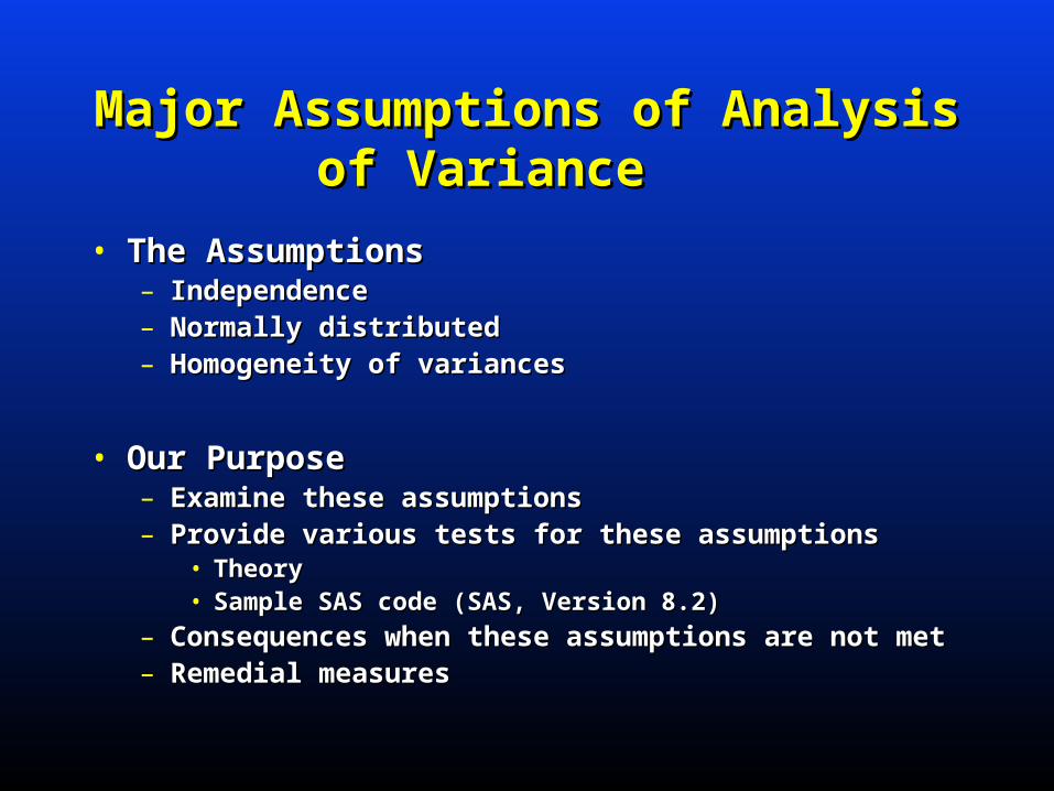
• The AssumptionsThe Assumptions– IndependenceIndependence– Normally distributedNormally distributed– Homogeneity of variancesHomogeneity of variances
• Our PurposeOur Purpose– Examine these assumptionsExamine these assumptions– Provide various tests for these assumptions Provide various tests for these assumptions
• TheoryTheory• Sample SAS code (SAS, Version 8.2) Sample SAS code (SAS, Version 8.2)
– Consequences when these assumptions are not metConsequences when these assumptions are not met– Remedial measuresRemedial measures
NormalityNormality
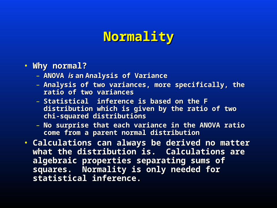
• Why normal?Why normal?– ANOVA ANOVA is is anan Analysis of Variance Analysis of Variance – Analysis of two variances, more specifically, the ratio of Analysis of two variances, more specifically, the ratio of
two variancestwo variances– Statistical inference is based on the F distribution Statistical inference is based on the F distribution
which is given by the ratio of two chi-squared which is given by the ratio of two chi-squared distributionsdistributions
– No surprise that each variance in the ANOVA ratio come No surprise that each variance in the ANOVA ratio come from a parent normal distributionfrom a parent normal distribution
• Calculations can always be derived no matter Calculations can always be derived no matter what the distribution is. Calculations are what the distribution is. Calculations are algebraic properties separating sums of squares. algebraic properties separating sums of squares. Normality is only needed for statistical inference.Normality is only needed for statistical inference.

NormalityNormalityTestsTests
• Wide variety of tests we can perform to test if the Wide variety of tests we can perform to test if the data follows a normal distribution. data follows a normal distribution.
• Mardia (1980) provides an extensive list for both Mardia (1980) provides an extensive list for both the univariate and multivariate cases, the univariate and multivariate cases, categorizing them into two types categorizing them into two types – Properties of normal distribution, more specifically, the Properties of normal distribution, more specifically, the
first four moments of the normal distribution first four moments of the normal distribution • Shapiro-Wilk’s W (compares the ratio of the standard Shapiro-Wilk’s W (compares the ratio of the standard
deviation to the variance multiplied by a constant to one)deviation to the variance multiplied by a constant to one)
– Goodness-of-fit tests, Goodness-of-fit tests, • Kolmogorov-Smirnov D Kolmogorov-Smirnov D • Cramer-von Mises WCramer-von Mises W22 • Anderson-Darling AAnderson-Darling A22

NormalityNormalityTestsTests
procproc univariateunivariate data=temp data=temp normal plotnormal plot;;
var expvar;var expvar;
runrun;;
procproc univariateunivariate data=temp data=temp normal plotnormal plot;;
var normvar;var normvar;
runrun;;
Tests for Normality
Test --Statistic--- -----p Value------
Shapiro-Wilk W 0.731203 Pr < W <0.0001
Kolmogorov-Smirnov D 0.206069 Pr > D <0.0100
Cramer-von Mises W-Sq 1.391667 Pr > W-Sq <0.0050
Anderson-Darling A-Sq 7.797847 Pr > A-Sq <0.0050
Tests for Normality
Test --Statistic--- -----p Value------
Shapiro-Wilk W 0.989846 Pr < W 0.6521
Kolmogorov-Smirnov D 0.057951 Pr > D >0.1500
Cramer-von Mises W-Sq 0.03225 Pr > W-Sq >0.2500
Anderson-Darling A-Sq 0.224264 Pr > A-Sq >0.2500
Normal Probability Plot 2.3+ ++ * | ++* | +** | +** | **** | *** | **+ | ** | *** | **+ | *** 0.1+ *** | ** | *** | *** | ** | +*** | +** | +** | **** | ++ | +* -2.1+*++ +----+----+----+----+----+----+----+----+----+----+
-2 -1 0 +1 +2
Stem Leaf # Boxplot 22 1 1 | 20 7 1 | 18 90 2 | 16 047 3 | 14 6779 4 | 12 469002 6 | 10 2368 4 | 8 005546 6 +-----+ 6 228880077 9 | | 4 5233446 7 | | 2 3458447 7 *-----* 0 366904459 9 | + | -0 52871 5 | | -2 884318651 9 | | -4 98619 5 +-----+ -6 60 2 | -8 98557220 8 | -10 963 3 | -12 584 3 | -14 853 3 | -16 0 1 | -18 4 1 | -20 8 1 | ----+----+----+----+ Multiply Stem.Leaf by 10**-1
Normal Probability Plot
8.25+
| *
|
|
| *
|
| *
| +
4.25+ ** ++++
| ** +++
| *+++
| +++*
| ++****
| ++++ **
| ++++*****
| ++******
0.25+* * ******************
+----+----+----+----+----+----+----+----+----+----+
Stem Leaf # Boxplot 8 0 1 * 7 7 6 6 1 1 * 5 5 2 1 * 4 5 1 0 4 4 1 0 3 588 3 0 3 3 1 0 2 59 2 | 2 00112234 8 | 1 56688 5 | 1 00011122223444 14 +--+--+ 0 55555566667777778999999 23 *-----* 0 000011111111111112222222233333334444444 39 +-----+ ----+----+----+----+----+----+----+----
Consequences of Non-NormalityConsequences of Non-Normality
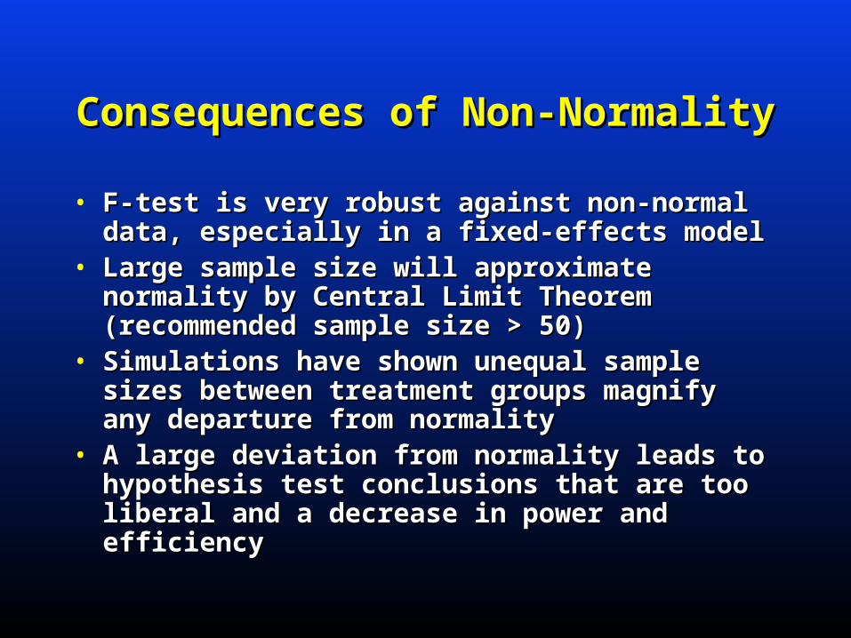
• F-test is very robust against non-normal data, F-test is very robust against non-normal data, especially in a fixed-effects modelespecially in a fixed-effects model
• Large sample size will approximate normality by Large sample size will approximate normality by Central Limit Theorem (recommended sample Central Limit Theorem (recommended sample size > 50) size > 50)
• Simulations have shown unequal sample sizes Simulations have shown unequal sample sizes between treatment groups magnify any departure between treatment groups magnify any departure from normalityfrom normality
• A large deviation from normality leads to A large deviation from normality leads to hypothesis test conclusions that are too liberal hypothesis test conclusions that are too liberal and a decrease in power and efficiencyand a decrease in power and efficiency
Remedial Measures for Non-Remedial Measures for Non-NormalityNormality
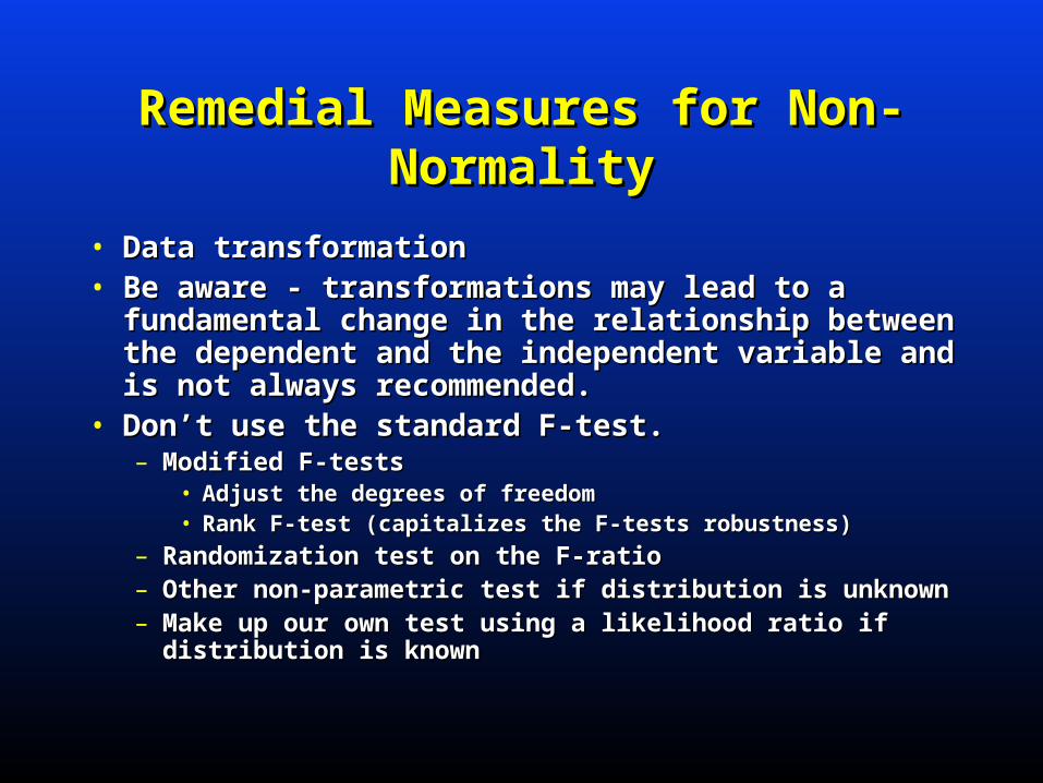
• Data transformationData transformation• Be aware - transformations may lead to a Be aware - transformations may lead to a
fundamental change in the relationship between the fundamental change in the relationship between the dependent and the independent variable and is not dependent and the independent variable and is not always recommended. always recommended.
• Don’t use the standard F-test. Don’t use the standard F-test. – Modified F-testsModified F-tests
• Adjust the degrees of freedomAdjust the degrees of freedom• Rank F-test (capitalizes the F-tests robustness)Rank F-test (capitalizes the F-tests robustness)
– Randomization test on the F-ratio Randomization test on the F-ratio – Other non-parametric test if distribution is unknownOther non-parametric test if distribution is unknown– Make up our own test using a likelihood ratio if distribution Make up our own test using a likelihood ratio if distribution
is known is known
IndependenceIndependence
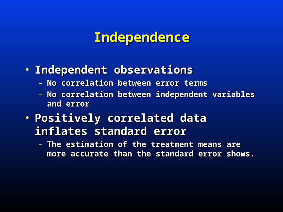
• Independent observationsIndependent observations– No correlation between error termsNo correlation between error terms– No correlation between independent variables and errorNo correlation between independent variables and error
• Positively correlated data inflates Positively correlated data inflates standard errorstandard error– The estimation of the treatment means are more The estimation of the treatment means are more
accurate than the standard error shows. accurate than the standard error shows.
Independence TestsIndependence Tests
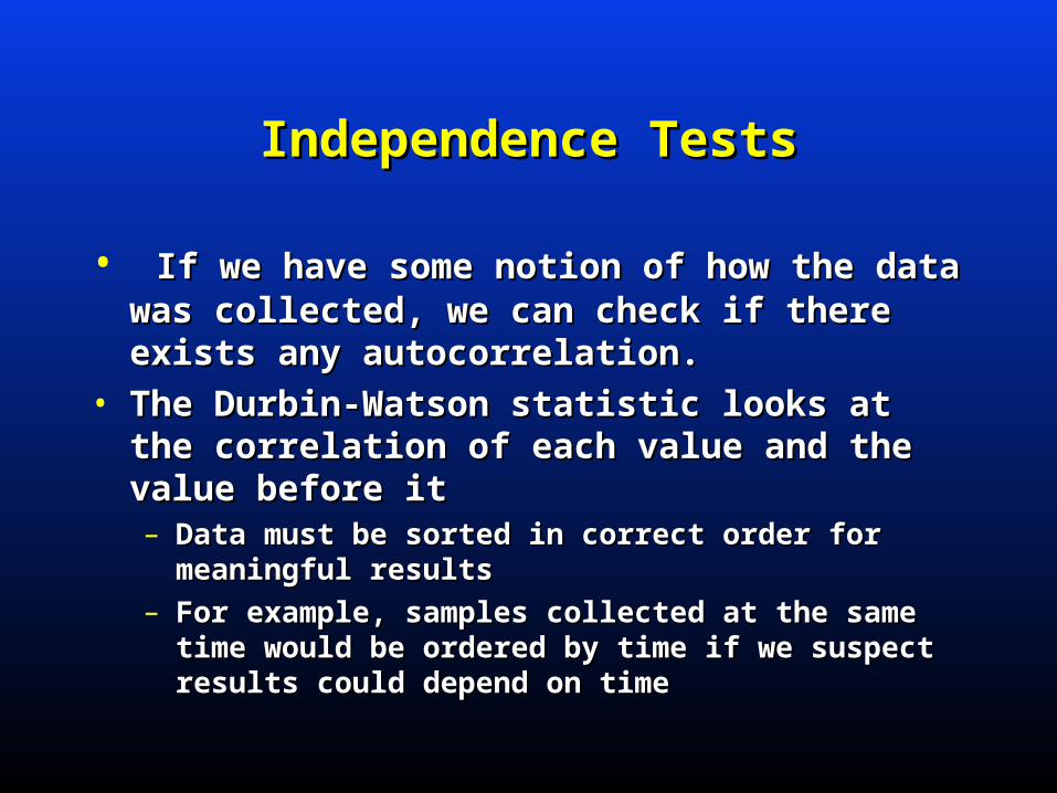
• If we have some notion of how the data was If we have some notion of how the data was collected, we can check if there exists any collected, we can check if there exists any autocorrelation. autocorrelation.
• The Durbin-Watson statistic looks at the The Durbin-Watson statistic looks at the correlation of each value and the value before itcorrelation of each value and the value before it– Data must be sorted in correct order for meaningful Data must be sorted in correct order for meaningful
resultsresults– For example, samples collected at the same time would For example, samples collected at the same time would
be ordered by time if we suspect results could depend be ordered by time if we suspect results could depend on timeon time
Independence TestsIndependence Tests
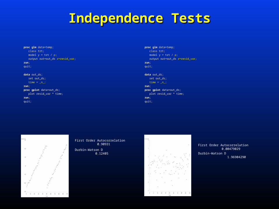
procproc glmglm data=temp; data=temp;
class trt;class trt;
model y = trt / model y = trt / pp;;
output out=out_ds output out=out_ds r=resid_varr=resid_var;;
runrun;;
quit;quit;
datadata out_ds; out_ds;
set out_ds;set out_ds;
time = _n_;time = _n_;
runrun;;
procproc gplotgplot data=out_ds; data=out_ds;
plot resid_var * time;plot resid_var * time;
runrun;;
quit;quit;
First Order Autocorrelation 0.00479029
Durbin-Watson D 1.96904290
First Order Autocorrelation 0.90931
Durbin-Watson D 0.12405
Remedial Measures for Dependent Remedial Measures for Dependent DataData
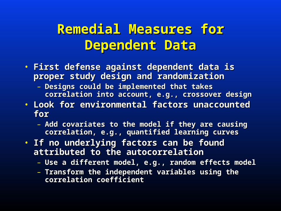
• First defense against dependent data is proper First defense against dependent data is proper study design and randomizationstudy design and randomization– Designs could be implemented that takes correlation Designs could be implemented that takes correlation
into account, e.g., crossover design into account, e.g., crossover design
• Look for environmental factors unaccounted forLook for environmental factors unaccounted for – Add covariates to the model if they are causing Add covariates to the model if they are causing
correlation, e.g., quantified learning curvescorrelation, e.g., quantified learning curves
• If no underlying factors can be found attributed to If no underlying factors can be found attributed to the autocorrelationthe autocorrelation– Use a different model, e.g., random effects modelUse a different model, e.g., random effects model– Transform the independent variables using the Transform the independent variables using the
correlation coefficientcorrelation coefficient
Homogeneity of VariancesHomogeneity of Variances
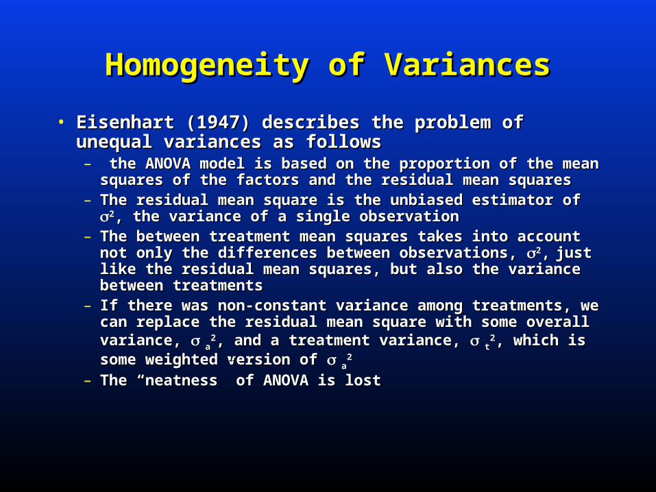
• Eisenhart (1947) describes the problem of unequal Eisenhart (1947) describes the problem of unequal variances as followsvariances as follows– the ANOVA model is based on the proportion of the mean the ANOVA model is based on the proportion of the mean
squares of the factors and the residual mean squares squares of the factors and the residual mean squares – The residual mean square is the unbiased estimator of The residual mean square is the unbiased estimator of 22, the , the
variance of a single observation variance of a single observation – The between treatment mean squares takes into account not The between treatment mean squares takes into account not
only the differences between observations, only the differences between observations, 22,, just like the just like the residual mean squares, but also the variance between residual mean squares, but also the variance between treatments treatments
– If there was non-constant variance among treatments, we can If there was non-constant variance among treatments, we can replace the residual mean square with some overall variance, replace the residual mean square with some overall variance,
aa22, and a treatment variance, , and a treatment variance, t t
22, which is some weighted , which is some weighted version of version of a a
22
– The “neatness” of ANOVA is lost The “neatness” of ANOVA is lost
Homogeneity of VariancesHomogeneity of Variances
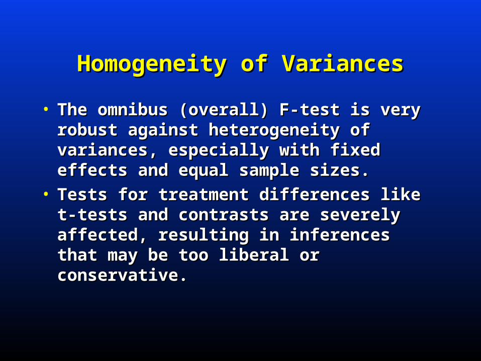
• The omnibus (overall) F-test is very robust The omnibus (overall) F-test is very robust against heterogeneity of variances, against heterogeneity of variances, especially with fixed effects and equal especially with fixed effects and equal sample sizes. sample sizes.
• Tests for treatment differences like t-tests Tests for treatment differences like t-tests and contrasts are severely affected, and contrasts are severely affected, resulting in inferences that may be too resulting in inferences that may be too liberal or conservative. liberal or conservative.
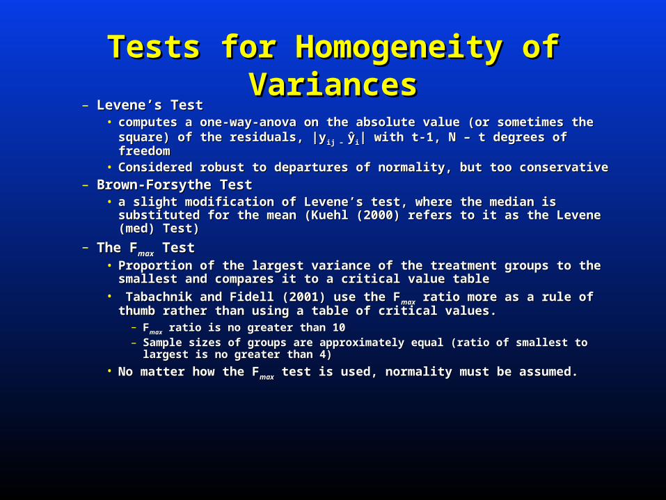
Tests for Homogeneity of VariancesTests for Homogeneity of Variances– Levene’s Test Levene’s Test
• computes a one-way-anova on the absolute value (or sometimes the computes a one-way-anova on the absolute value (or sometimes the square) of the residuals, |ysquare) of the residuals, |y
ij – ij – ŷŷii| with t-1, N – t degrees of freedom| with t-1, N – t degrees of freedom• Considered robust to departures of normality, but too conservativeConsidered robust to departures of normality, but too conservative
– Brown-Forsythe Test Brown-Forsythe Test • a slight modification of Levene’s test, where the median is substituted a slight modification of Levene’s test, where the median is substituted
for the mean (Kuehl (2000) refers to it as the Levene (med) Test)for the mean (Kuehl (2000) refers to it as the Levene (med) Test)
– The FThe Fmaxmax Test Test • Proportion of the largest variance of the treatment groups to the Proportion of the largest variance of the treatment groups to the
smallest and compares it to a critical value tablesmallest and compares it to a critical value table• Tabachnik and Fidell (2001) use the FTabachnik and Fidell (2001) use the F
maxmax ratio more as a rule of thumb ratio more as a rule of thumb rather than using a table of critical values. rather than using a table of critical values.
– FFmaxmax ratio is no greater than 10 ratio is no greater than 10 – Sample sizes of groups are approximately equal (ratio of smallest to largest Sample sizes of groups are approximately equal (ratio of smallest to largest
is no greater than 4) is no greater than 4)
• No matter how the FNo matter how the Fmaxmax test is used, normality must be assumed. test is used, normality must be assumed.
Tests for Homogeneity of VariancesTests for Homogeneity of Variances
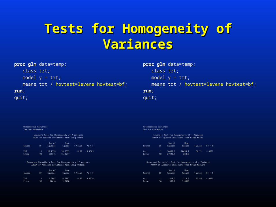
procproc glmglm data=temp; data=temp;
class trt;class trt;
model y = trt;model y = trt;
means trt / means trt / hovtest=levene hovtest=bfhovtest=levene hovtest=bf;;
runrun;;
quit;quit;
procproc glmglm data=temp; data=temp;
class trt;class trt;
model y = trt;model y = trt;
means trt / means trt / hovtest=levene hovtest=bfhovtest=levene hovtest=bf;;
runrun;;
quit;quit;
Homogeneous Variances
The GLM Procedure
Levene's Test for Homogeneity of Y Variance
ANOVA of Squared Deviations from Group Means
Sum of Mean
Source DF Squares Square F Value Pr > F
TRT 1 10.2533 10.2533 0.60 0.4389
Error 98 1663.5 16.9747
Brown and Forsythe's Test for Homogeneity of Y Variance
ANOVA of Absolute Deviations from Group Medians
Sum of Mean
Source DF Squares Square F Value Pr > F
TRT 1 0.7087 0.7087 0.56 0.4570
Error 98 124.6 1.2710
Heterogenous Variances
The GLM Procedure
Levene's Test for Homogeneity of y Variance
ANOVA of Squared Deviations from Group Means
Sum of Mean
Source DF Squares Square F Value Pr > F
trt 1 10459.1 10459.1 36.71 <.0001
Error 98 27921.5 284.9
Brown and Forsythe's Test for Homogeneity of y Variance
ANOVA of Absolute Deviations from Group Medians
Sum of Mean
Source DF Squares Square F Value Pr > F
trt 1 318.3 318.3 93.45 <.0001
Error 98 333.8 3.4065
Tests for Homogeneity of VariancesTests for Homogeneity of Variances
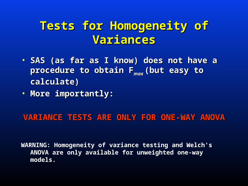
• SAS (as far as I know) does not have a procedure SAS (as far as I know) does not have a procedure to obtain to obtain FFmax max (but easy to calculate)(but easy to calculate)
• More importantly:More importantly:
VARIANCE TESTS ARE ONLY FOR ONE-WAY VARIANCE TESTS ARE ONLY FOR ONE-WAY ANOVAANOVA
WARNING: Homogeneity of variance testing and Welch's ANOVA are only available for unweighted one-way models.
Tests for Homogeneity of VariancesTests for Homogeneity of Variances(Randomized Complete Block Design and/or (Randomized Complete Block Design and/or
Factorial Design)Factorial Design)
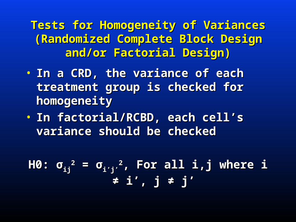
• In a CRD, the variance of each treatment In a CRD, the variance of each treatment group is checked for homogeneitygroup is checked for homogeneity
• In factorial/RCBD, each cell’s variance In factorial/RCBD, each cell’s variance should be checkedshould be checked
H0: σH0: σijij22 = σ = σi’j’i’j’
22, For all i,j where i ≠ i’, j ≠ j’, For all i,j where i ≠ i’, j ≠ j’
Tests for Homogeneity of VariancesTests for Homogeneity of Variances(Randomized Complete Block Design and/or (Randomized Complete Block Design and/or
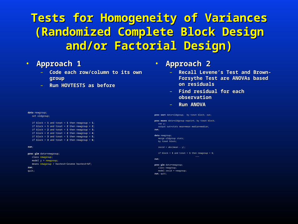
Factorial Design)Factorial Design)• Approach 1Approach 1
– Code each row/column to its own Code each row/column to its own groupgroup
– Run HOVTESTS as beforeRun HOVTESTS as before
• Approach 2Approach 2– Recall Levene’s Test and Recall Levene’s Test and Brown-Brown-
Forsythe Test are ANOVAs based on Forsythe Test are ANOVAs based on residualsresiduals
– Find residual for each observationFind residual for each observation– Run ANOVARun ANOVA
datadata newgroup; newgroup;
set oldgroup;set oldgroup;
if block = if block = 11 and treat = and treat = 11 then newgroup = then newgroup = 11;;
if block = if block = 11 and treat = and treat = 22 then newgroup = then newgroup = 22;;
if block = if block = 22 and treat = and treat = 11 then newgroup = then newgroup = 33;;
if block = if block = 22 and treat = and treat = 22 then newgroup = then newgroup = 44;;
if block = if block = 33 and treat = and treat = 11 then newgroup = then newgroup = 55;;
if block = if block = 33 and treat = and treat = 22 then newgroup = then newgroup = 66;;
runrun;;
procproc glmglm data=newgroup; data=newgroup;
class class newgroupnewgroup;;
model y = model y = newgroupnewgroup;;
means means newgroupnewgroup / hovtest=levene hovtest=bf; / hovtest=levene hovtest=bf;
runrun;;
quit;quit;
procproc sortsort data=oldgroup; by treat block; run; data=oldgroup; by treat block; run;
procproc meansmeans data=oldgroup noprint; by treat block; data=oldgroup noprint; by treat block;
var y;var y;
output out=stats mean=mean median=median;output out=stats mean=mean median=median;
runrun;;
datadata newgroup; newgroup;
merge oldgroup stats;merge oldgroup stats;
by treat block;by treat block;
resid = abs(mean - y);resid = abs(mean - y);
if block = if block = 11 and treat = and treat = 11 then newgroup = then newgroup = 11;;
……… ………
runrun;;
procproc glmglm data=newgroup; data=newgroup;
class newgroup;class newgroup;
model resid = newgroup;model resid = newgroup;
runrun; quit;; quit;
Tests for Homogeneity of VariancesTests for Homogeneity of Variances(Repeated-Measures Design)(Repeated-Measures Design)
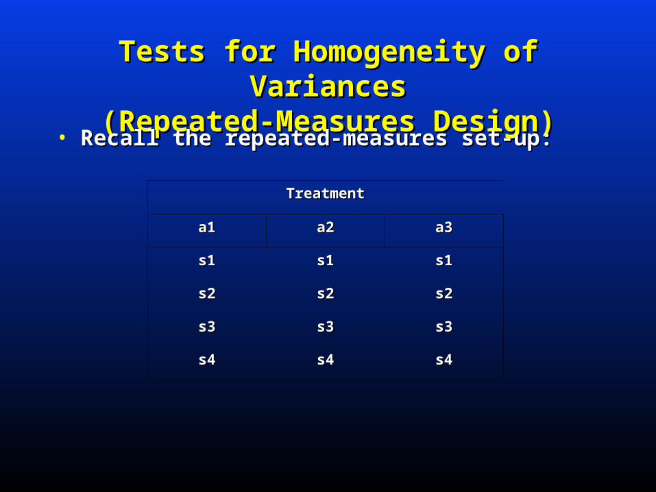
• Recall the repeated-measures set-up:Recall the repeated-measures set-up:
TreatmentTreatment
a1a1 a2a2 a3a3
s1s1 s1s1 s1s1
s2s2 s2s2 s2s2
s3s3 s3s3 s3s3
s4s4 s4s4 s4s4
Tests for Homogeneity of VariancesTests for Homogeneity of Variances(Repeated-Measures Design)(Repeated-Measures Design)
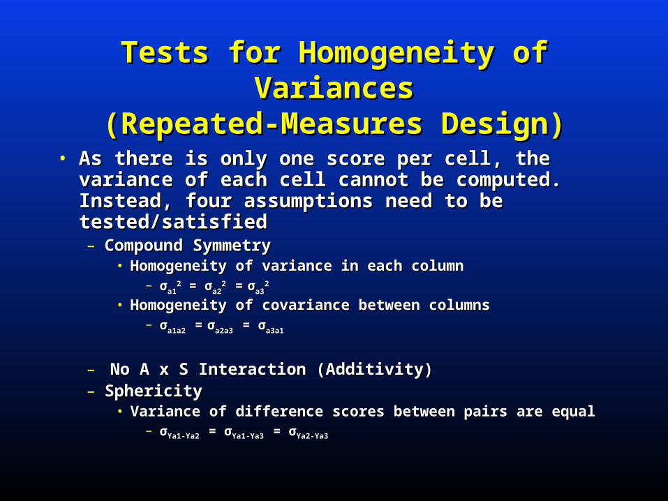
• As there is only one score per cell, the variance As there is only one score per cell, the variance of each cell cannot be computed. Instead, four of each cell cannot be computed. Instead, four assumptions need to be tested/satisfiedassumptions need to be tested/satisfied– Compound SymmetryCompound Symmetry
• Homogeneity of variance in each column Homogeneity of variance in each column – σσa1a1
22 = σ = σa2a22 2 == σσa3a3
2 2
• Homogeneity of covariance between columnsHomogeneity of covariance between columns– σσa1a2a1a2
== σσa2a3a2a3 = σ= σa3a1a3a1
– No A x S Interaction (Additivity)No A x S Interaction (Additivity)– SphericitySphericity
• Variance of difference scores between pairs are equalVariance of difference scores between pairs are equal– σσYYa1-Ya2a1-Ya2
= σ= σYYa1-Ya3a1-Ya3 = σ= σYYa2-Ya3a2-Ya3
Tests for Homogeneity of VariancesTests for Homogeneity of Variances(Repeated-Measures Design)(Repeated-Measures Design)
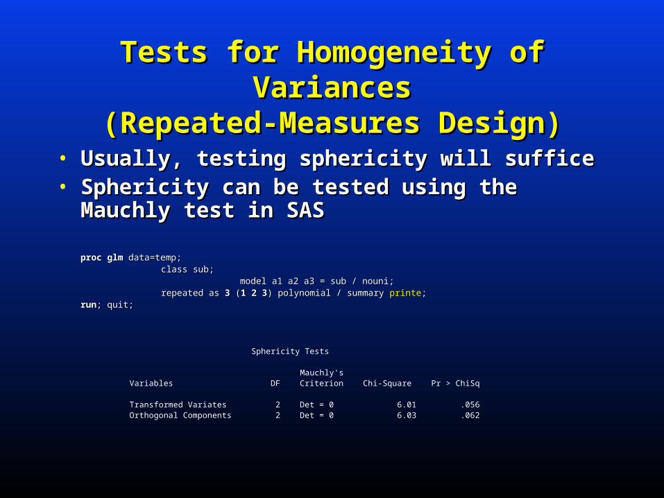
• Usually, testing sphericity will suffice Usually, testing sphericity will suffice • Sphericity can be tested using the Mauchly test in Sphericity can be tested using the Mauchly test in
SASSAS
procproc glmglm data=temp; data=temp; class sub;class sub;
model a1 a2 a3 = sub / nouni;model a1 a2 a3 = sub / nouni; repeated as repeated as 33 ( (11 22 33) polynomial / summary ) polynomial / summary printeprinte;; runrun; quit;; quit;
Sphericity Tests
Mauchly's Variables DF Criterion Chi-Square Pr > ChiSq
Transformed Variates 2 Det = 0 6.01 .056 Orthogonal Components 2 Det = 0 6.03 .062
Tests for Homogeneity of VariancesTests for Homogeneity of Variances(Latin-Squares/Split-Plot Design)(Latin-Squares/Split-Plot Design)
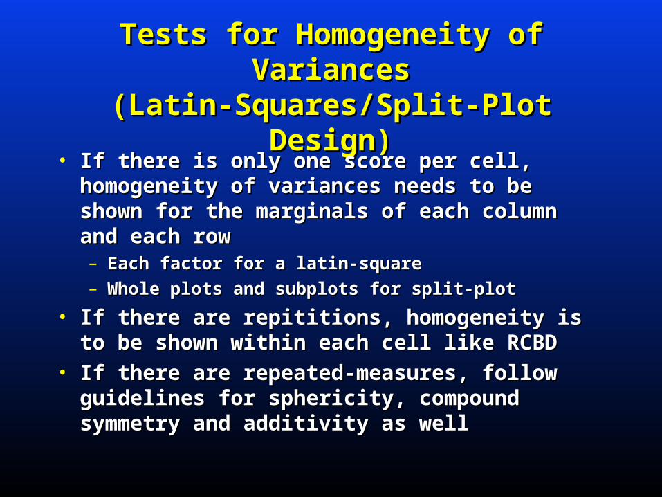
• If there is only one score per cell, homogeneity of If there is only one score per cell, homogeneity of variances needs to be shown for the marginals of variances needs to be shown for the marginals of each column and each roweach column and each row– Each factor for a latin-squareEach factor for a latin-square– Whole plots and subplots for split-plot Whole plots and subplots for split-plot
• If there are repititions, homogeneity is to be If there are repititions, homogeneity is to be shown within each cell like RCBDshown within each cell like RCBD
• If there are repeated-measures, follow guidelines If there are repeated-measures, follow guidelines for sphericity, compound symmetry and additivity for sphericity, compound symmetry and additivity as wellas well
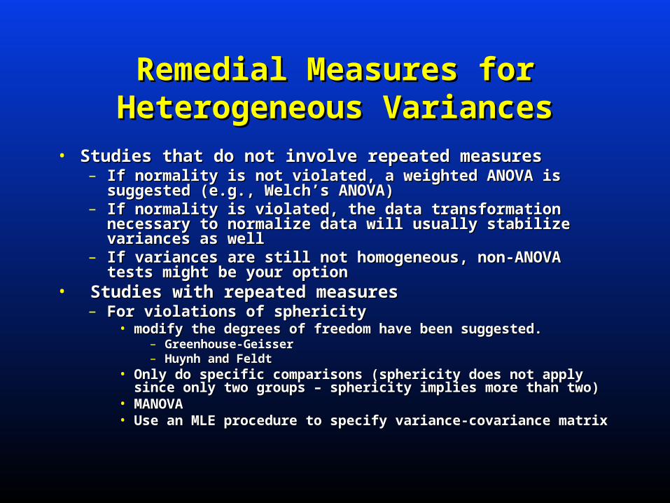
Remedial Measures for Remedial Measures for Heterogeneous VariancesHeterogeneous Variances
• Studies that do not involve repeated measuresStudies that do not involve repeated measures– If normality is not violated, a weighted ANOVA is suggested If normality is not violated, a weighted ANOVA is suggested
(e.g., Welch’s ANOVA)(e.g., Welch’s ANOVA)– If normality is violated, the data transformation necessary to If normality is violated, the data transformation necessary to
normalize data will usually stabilize variances as wellnormalize data will usually stabilize variances as well– If variances are still not homogeneous, non-ANOVA tests If variances are still not homogeneous, non-ANOVA tests
might be your optionmight be your option• Studies with repeated measuresStudies with repeated measures
– For violations of sphericityFor violations of sphericity• modify the degrees of freedom have been suggested.modify the degrees of freedom have been suggested.
– Greenhouse-Geisser Greenhouse-Geisser – Huynh and FeldtHuynh and Feldt
• Only do specific comparisons (sphericity does not apply since Only do specific comparisons (sphericity does not apply since only two groups – sphericity implies more than two)only two groups – sphericity implies more than two)
• MANOVAMANOVA• Use an MLE procedure to specify variance-covariance matrix Use an MLE procedure to specify variance-covariance matrix
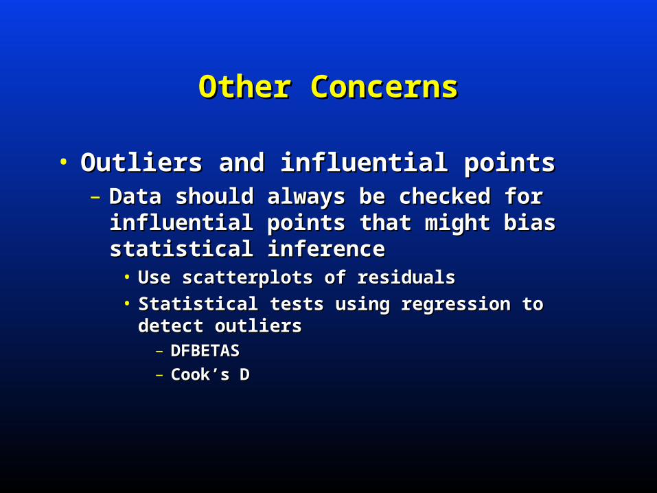
Other ConcernsOther Concerns
• Outliers and influential pointsOutliers and influential points– Data should always be checked for influential Data should always be checked for influential
points that might bias statistical inferencepoints that might bias statistical inference• Use scatterplots of residualsUse scatterplots of residuals• Statistical tests using regression to detect outliersStatistical tests using regression to detect outliers
– DFBETASDFBETAS
– Cook’s DCook’s D
ReferencesReferences• Casella, G. and Berger, R. (2002). Casella, G. and Berger, R. (2002). Statistical InferenceStatistical Inference. United States: Duxbury.. United States: Duxbury.
• Cochran, W. G. (1947). Some Consequences When the Assumptions for the Analysis of Cochran, W. G. (1947). Some Consequences When the Assumptions for the Analysis of Variances are not Satisfied. Variances are not Satisfied. BiometricsBiometrics. Vol. 3, 22-38.. Vol. 3, 22-38.
• Eisenhart, C. (1947). The Assumptions Underlying the Analysis of Variance. Eisenhart, C. (1947). The Assumptions Underlying the Analysis of Variance. BiometricsBiometrics. . Vol. 3, 1-21.Vol. 3, 1-21.
• Ito, P. K. (1980). Robustness of ANOVA and MANOVA Test Procedures. Ito, P. K. (1980). Robustness of ANOVA and MANOVA Test Procedures. Handbook of Handbook of Statistics 1: Analysis of Variance Statistics 1: Analysis of Variance (P. R. Krishnaiah, ed.), 199-236. Amsterdam: North-(P. R. Krishnaiah, ed.), 199-236. Amsterdam: North-Holland.Holland.
• Kaskey, G., et al. (1980). Transformations to Normality. Kaskey, G., et al. (1980). Transformations to Normality. Handbook of Statistics 1: Analysis Handbook of Statistics 1: Analysis
of Variance of Variance (P. R. Krishnaiah, ed.), 321-341. Amsterdam: North-Holland.(P. R. Krishnaiah, ed.), 321-341. Amsterdam: North-Holland.
• Kuehl, R. (2000). Kuehl, R. (2000). Design of Experiments: Statistical Principles of Research Design and Design of Experiments: Statistical Principles of Research Design and AnalysisAnalysis, 2nd edition. United States: Duxbury., 2nd edition. United States: Duxbury.
• Kutner, M. H., et al. (2005). Kutner, M. H., et al. (2005). Applied Linear Statistical ModelsApplied Linear Statistical Models, 5th edition. New York: , 5th edition. New York: McGraw-Hill.McGraw-Hill.
• Mardia, K. V. (1980). Tests of Univariate and Multivariate Normality. Mardia, K. V. (1980). Tests of Univariate and Multivariate Normality. Handbook of Statistics Handbook of Statistics 1: Analysis of Variance 1: Analysis of Variance (P. R. Krishnaiah, ed.), 279-320. Amsterdam: North-Holland.(P. R. Krishnaiah, ed.), 279-320. Amsterdam: North-Holland.
• Tabachnik, B. and Fidell, L. (2001). Tabachnik, B. and Fidell, L. (2001). Computer-Assisted Research Design and AnalysisComputer-Assisted Research Design and Analysis. . Boston: Allyn & Bacon.Boston: Allyn & Bacon.