BUREAU OF THE CENSUS

STATISTICAL RESEARCH DIVISION REPORT SERIES

SRD Research Report Number: CENSUS/SRD/RR-86/10

THE ASYMPTOTIC DISTRIBUTION OF THE LIKELIHOOD RATIO TEST FOR A

CHANGE IN THE MEAN

John M. Irvine* Bureau of the Census

Washington, D.C. 20233

This series contains research reports, written by or in cooperation with staff members of the Statistical Research Division, whose content may be of interest to the general statistical research community. The views re- flected in these reports are not necessarily those of the Census Bureau nor do they necessarily represent Census Bureau statistical policy or prac- tice. Inquiries may be addressed to the author(s) or the SRD Report Series Coordinator, Statistical Research Division, Bureau of the Census, Washington, D.C. 20233.

Recommended by: David F. Findley

Report completed: March 25, 1986

Report issued: March 25, 1986

*Former ASA/NSF/Census Junior Fellow

The Asymptotic Distribution of

The Likelihood Ratio Test for a

Change in the Mean

Abbreviated Title: Likelihood Ratio Test for Change

John M. Xrvine

Summary

A likelihood ratio test is one technique for

detecting a shift in the mean of a sequence of independent

* normal random variables. If the time of the possible

change is unknown, the asymptotic null distribution of the *

test statistic is extreme value, rather than the usual

chi-square distribution. The asymptotic distribution is

derived here under the null hypothesis of no change.

Keywords

asymptotic distribution, changepoint, extreme-value

distribution, likelihood ratio test

i

1. Introduction

This discussion

change in the mean

examines the problem of testing for a

of a sequence of independent normal

variates, where the time of a possible change is

unknown. The asymptotic distribution of the likelihood

ratio statistic is derived. Shaban (1980) presents a

bibliography of related problems.

Let Ylr Y,, . . . . Y L1 be independent normal random I L L"

* 2 variables with means pi and equal variance u .

* ential question under consideration is to test

for all i; against Hl: pi = ~1 for i 5 v and Ui

> v is unknown. Calculation of the likelihood

tistic X for this problem is straight-forward

The infer-

Ho: "i = ~

= u 2 for i

ratio sta-

and can be

found in Hawkins (1977). Using a recursive integral equa- .

tion, Hawkins produces a table of fractiles for the like-

lihood ratio statistic. Arguing heuristically, he asserts

that (-2 log ,)112 converges to an extreme value distribu-

tion. Unfortunately the heuristic argument does not yield

the correct normalizing constants for the distribution.

The asymptotic result presented here resolves this

question.

1

2. The Asymptotic Distribution

Let Yl, . . . . YN be as in the previous section and

consider the testing problem presented. First examine the

case where u 2 is known and, without loss of generality,

let a2 = 1. Define

N so= c (Yi-e)2

i-l

sp = z iv1 fY i - p,,2 + c is:+, (' i

- p,j2 =

*

where

5i = (l/N) : Y. i=l '

V

F, = (l/v) c Y.

i=l l

I;2 = [l/(N - ~11 !f Y

i=v+l i

Note that So is the residual sum of squares under Ho

and sl(v) is the residual sum of squares under Hl given

V. Then the likelihood ratio statistic X can be written

as

2

.

(2.1) -2 log X = So - inf lLv<N

SIW

When u 2 unknown, the likelihood ratio statistic is

x = inf [ sO -N/2

llv<N S,(d

For u 2 known the asymptotic null distribution of -2 log X

is given by:

* Theorem 2.1: Let -2 log 1 be as in equation (2.1) and

suppose Ho is true. Then

( -2 lCXJ A)v2 < (2 log lq N)V2 +- lsq log N 2(2 leg log NI I.0

6

+

(2 lcqwlcq N)1'2 ] = exp[ $21

Proof: Several lemmas are needed to establish the theo-

rem.

Lemma 2.2: For the testing problem under consideration:

v

2

-2 log A = max 1

lLv<N (' - v/N) (v/N)

3

.

where yi = 'i - ,.

Proof of lemma: Follows directly from (2.1).

The next lemma will utilize the properties of the

Ornstein-Uhlenbeck process and Brownian bridge.

Definition 2.3: A continuous stochastic process U(t) is

called an Ornstein-Uhlenbeck process if U(t) is station-

ary, Markov and Gaussian with E[U(t)] = 0 and Cov [U(t),

U(s)1 =exp(- t- I s/) for any real t and s. .

Definition 2.4:

a [O,l] is called

where B(t) is a

Lemma 2.5: Let

* WN =

A continuous Gaussian process Be(t) on

a Brownian bridqe if Be(t) = B(t) - tB(1)

standard Brownian motion on [O,l].

y1* . . . . yN be defined as above and let

sup, IU(s) I SE s

N

where U(s) is an Ornstein-Uhlenbeck process and SN+ is a

set defined below. Then Wi has the same distribution as

(-2 log IP2

Proof of lemma:

The result will be established by comparing (-2 log

AY2 to a Brownian bridge, which is related to the

Ornstein-Uhlenbeck process by a simple transformation.

The definition of S+ N

will be constructed in the process.

d

i

.

First note

V V N 1 yi = C e. - (v/N) C e.

i=l i=l l i=l '

where ei - i.i.d. N(O,l), i=l, . . . . N. Since ei is

Gaussian, (N -l/2 py 1 if v = 1, . . . . N-1) and CBO(t), tcTN}

have the same joint distribution where

TN = N-l

. . . . N

Similarly, the two sets of random variables {[(l - t) (t)1112

BO(t), teTN) and {[(l - v/N)(v/N)]~‘~ N’1’2 rVYi, v=l,

. . . . N-11 have the same joint distribution.

For the Brownian bridge there exists an Ornstein-

Uhlenbech process U(s) on the real line satisfying

BOW = [t (1-t)1’/2 U(( 1/2)log(&))

Let

sN = I S1 s = l/2 log (&I, n = I, . . . . N-1)

5

4

Then WN = sup [(1-t)tl-1’2 lB"(t) 1 has the same distribu-

tion as sup tETN )U(s) 1. sss

N

Define Si by

+ sN

= {s+ 1 s+ =: S + 1/2 logIN-1), stSNf

.

Then sup pm 1 and sup have the same distribu- SE: SN SOS

tion. Therefore (-2 log X)1'2 has the same

* distribution as Wi = sup IUls) 1. sg SN

Lemma 2.6: Let U(s) be an Ornstein-Uhlenbeck process

defined for s > 0. =

Then .

1imP (u(S)1 < (2 lag leg N)1’2 + 'log '=I 'Oq N N+ - O<s%q(N) 2(2 lq lq N)V2

+ (2lq 1~ NIV2

] =exp [.s]

Proof of Lemma:

Using some results from Darling and Erdos (1956), the

lemma follows easily. Let

T(a) = supttlU(r) < a, 0 2 T 2 t)

In other words T(a) is the time at which U(t) first

crosses a.

Darling and Erdos (1956) show that

lim P (2n)1'2

T(a) > a = e--z ea2/2Z

a + - 1 * And if

( 2R )1’2 ea2/2 2 = log N a II

then, as N * 0,

a = (2 log log N)1’2 + la3 103 la N cr;l (J2z)

2(2 lq lq N) l/2 -

(211~ lq NIV2

Combining these facts yield

7

.

lim P sup U(s) < a = T(a) > log N N* = O<s<log(N)

I 3

0-z = e 0-w -e = exp - [ 1 y2

where w = - log (II 1'22) . Using the above expression for a

produces:

lU(S)I < (2 leg loz~ N)V2 + ioq log lW N 2(2 iog iq NIV2

+

(2 leg ;q N)"2

The next lemma requires some additional notation:

I N-l

sK = l/2 log K -

N-K

N(a) = an integer such that U(SK) ( a, K < N(a)

U(SK) > a for K = N(a) =

K(a) is the integer such that Syta)-1 < T(a) 2 SKta) *

(Recall T(a) is the time U(t) first crosses a). L(a) = SK(a) - SK(a! i - 1

u(a) = (2n)1/2 ea2/2

a Lemma 2.7:

There exists a(N) a function of N such that

lim N+ 0 (2 iogahg N)i’2 = ’

and log N(a) / T(a) * 1 as N + a.

Proof of lemma:

* The lemma will be established by showing that P[K(a)

i N(a) < K(a+6)]+ 1 as N * -, where E is a suitable func- =:

tion of N. The lemma will follow from this expression.

Two results from Darling and Erdos (1956) are used:

1. lim PIT(a) > v(a)y] = coy a+-

2. I ( T a+e) - T(a) I + 0, as N - - where E = l/a2.

Note that N (a) > K(a) by definition, so it suffices Z

to show

(2.6) P[N(a) < K(a+B)j * 1 =

as E + 0, a + =. 2 Let E = l/a .

To establish (2.6)‘ calculate:

P(a) q =P N(a) > K(a+E) 1 T(a) > -

a

For K > 2 note (N-K+l)/(N-1) < K/(K-1) and (N-1)/(+ =

K) < K. =

Hence:

L(a) = SK(a) - ‘K(a) - 1

= -l/2 log '"(;JK;r;" I J

- l/2 log I

(K(a)-1) (N-1) N-K(a) + 1 J

g log K(a) - log(K(a) - 1)

2 2 K(a)

Also

T(a) 6 ‘K(a)

= l/2 log K(a) N-l

N-K(a)

=> l/K(a) < eBTta)

10

So for T(a) > u(a)/a this implies

L(a) $ 2 exp

= 2 exp

= $(a)

[ - (2n)‘/2/a ea2/2J

The event N (a) > K (a + 6) implies that U (t) having =

a reached a + B, has decreased below a in a time span less than +(a). Recalling that the Ornstein-Uhlenbeck process

is stationary:

Q 2 P[U(*(a)) < a 1 U(0) = a+c]

The conditional distribution of U(S(a)) given U(0) =

a + E is normal with mean (a + C) e -*(a) and variance

l,e-21da) < 2-+(a). Therefore s

q < (2uC2)-1'2 exp(-C2/2) =

where

11

= ja+c) e-Y(E) > (a+&) e -*v(a) E

o(a) = (2v(a))1’2

E ' 2($(a)J1'2

for a > a0

Since L = l/a, c/($(a)) l/2 * -, implying q + 0.

Setting y=l/a and using the result of Darling and

Erdos (1956) we see that P [T(a) > v(a)/a] + 1 as N * -=.

Hence P [K(a)<N(a)<K(a+c)] + 1. Further, note that the

* result of Darling and Erdos implies that T(a) * -, as a *

=+.

Now consider for a * - the equation: *

u(a) z = log N + z

The solution is

a = (2 kg icg N)1’2 + 1m ‘02 1a y,2 - ‘Oat PV2Z)

2t2 1~ la;~ N) (2loz~ 1~ NIV2

+o

, i

i

(2 1Og kg N)v2)

=> P [T(a) > log N] + e-' as N+-

12

.

.I.

=> T(a) = log N + OP(l)

Now recall

'K(a)-1 2 T(a) 2 S K(a)

N+l => (K(a)-1) N-K(a)+l = < e2T(a) < K(a) - ' = NyK(a)

*

For large N, (N-l)/(N-K(a)) G N/(N-K(a)). SO * .

e ZT(a) N 6 K(a) N-K(a)

= > K(a) < eZTta)/ 1 + e2i(a) =

Similarly

K(a) 5 e 2Tta)

.2T(a) /(I+ N 3+1

So for large N

K(a) = e 2T

2T(a) )/ (1 + e N 11-6 op<i

13

Substituting for T(a) implies that I N(a) - K(a)1 =

Gpw. Recalling

sK = l/2 log KN-K 1

N-l

we obtain

'K(a) = log K(a) + Op(l)

And T(a) + 61 = SKta) for 0 I, 61 < .l, implying T(a) = log

* K(a) - 61 + Op(l), for large N. Hence

loq K(a) ~ T(a)+6i+0p(l)

as N.+ -

Recalling expression (2.6) we obtain, for 0 < 62 < 1: =

P [K(a) s N(a) i K(a+f)] * 1

> P loq K(a) I

T(a)+61+Op(l) (T(a)+sl+Op(l)) $ 1Og N(a) ', T(a+;;9+gN$)(l) 2 P

(T(a+E)+S2+Op(l)) 1 + 1 => P

“1 -T(a)+

op T(a) 2

lot NW ( T;;-+;) + .A, + %? 1 + 1 T(a) = , L aI T(a) J

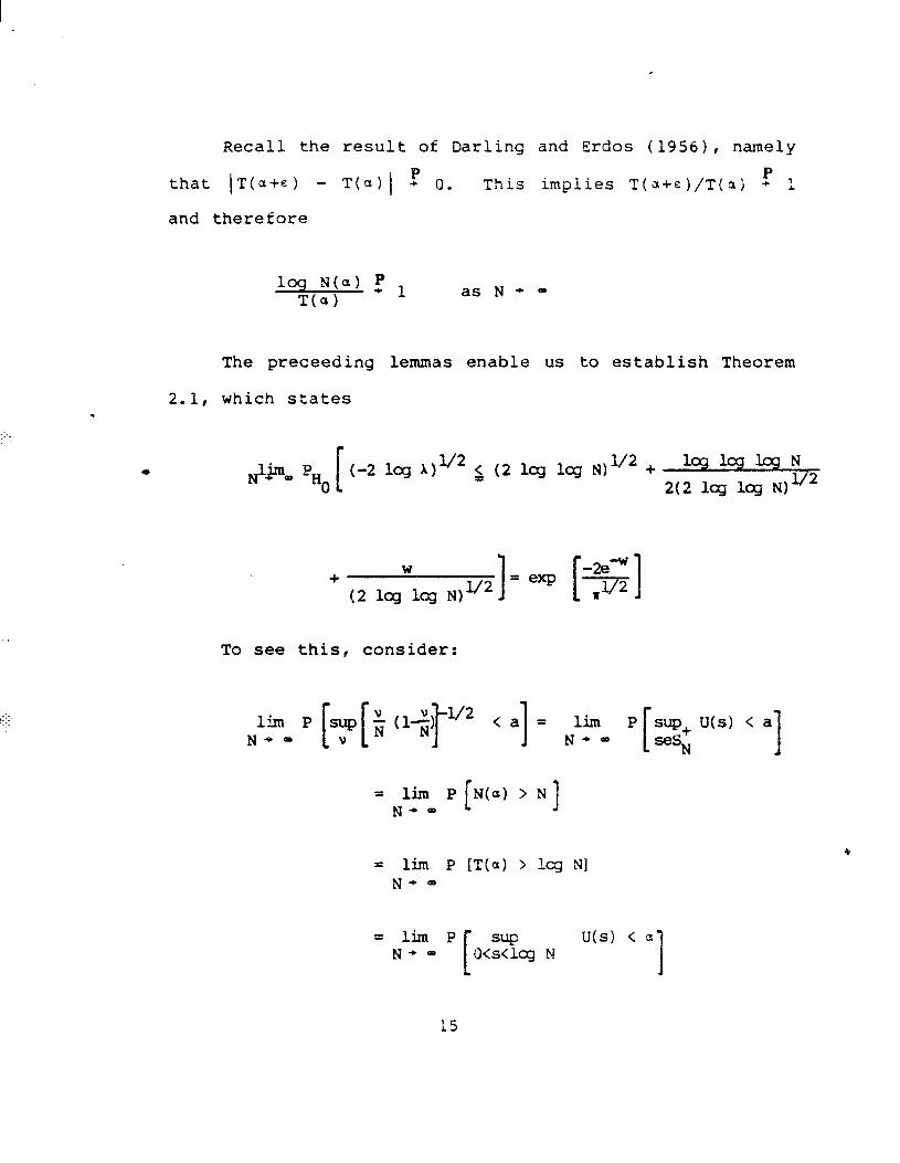
Recall the result of Darling and Erdos (1956), namely

that lT(a+e) - T(a)1 ! 0. This implies T(a+E)/T(a) -pl

and therefore

log N(a) ,p 1 T(a)

as N-c -

The preceeding

2.1, which states

lemmas enable us to establish Theorem

+ (2 lqwlq NIV2 ]=- [=fG]

To see this, consider:

= lb!i P N(a) > N N’ Q) I

= lim P [T(a) > kg N] N* -

= lim P U(s) < a N’- O<%J N 1

-2 =e

where

a = (2 kg log N) 1/2 + loa ku ~CQ N a (A2Z)

32 log lq N) m - (2tq kx~ N)V2

+o 1

(2 lq lq N)v2 *

Substituting w = -log(n l/2 z) and recalling

SUP -li2 f112 1; yi 1 = (-2 log 1)1'2 v 1

and

lim P SUP IU(SJl < a '= ea2' N+= ots<log N 1

yields the desired result.

For c2 unknown the same asymptotic distribution holds

under HO, as demonstrated by:

Theorem 2.7:

16

Let yl, . . . . YN * i.i.d. N(P, u2) and let

-N/2 a = min

lLv<N

Then

lim P (-2 leg X) l/2

N* - 921~331cgN)~~. '=?doqlqN 2

2(2 lq lq NIV

Proof of theorem:

Essentially -2 log X can be written as the sum of two

terms, one of which behaves asymptotically like -2 log X

when u 2 is known. The other term in Op ((log log N)/N)

and can be ignored.

Note:

-2 log A = sup lsv<N

- N log (S/So)

= sup v [ :"';;I + s:pN 0 (s:;1]2

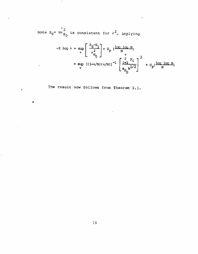
-2 Note So= NaH 2

0 is consistent for Q , implying

The result now follows from Theorem 2.1. .

Acknowledgements: This research was supported in part by

NSF Grant No. SOC 76-15271 and the LJS Census Bureau under

the American Statistical Association Fellowship Program.

This work is based on sections of the author's Ph.D.

dissertation (Yale 1982) and the author gratefully

acknowledges Professors F.J. Anscombe, John Hartigan and

David Pollard and Dr. David Findley for valuable advice

during its preparation.

19

REFERENCES

Darling, D.A. and Erdos, P. (1956). A limit theorem for the maximum of normalized sums of independent random variables. Duke Math. Journal, 23, 143-155.

Hawkins, D.M. (1977). Testing a sequence of observations for a shift in location. J. Amer. Statist. Assoc., 72, 180-186.

Shaban, S.A. (1980). Change point problems regression: an annotated bibliography. Statist. Rev., 48, 83-93.

and two-phase International

2 0