The Australian National University

Centre for Economic Policy Research DISCUSSION PAPER

Heterogeneity in the Returns to Investment in Poor Villages

Chikako Yamauchi

DISCUSSION PAPER NO. 582 July 2008

ISSN: 1442-8636 ISBN: 978 1 921262 57 9

Mailing address: Economics Program, RSSS, H.C. Coombs Bldg., The Australian National University, Canberra, ACT 2000, Australia; Telephone: +61-2-6125-2355; Fax: +61-2-6125-0182.

Acknowledgement: I am grateful to Duncan Thomas for his helpful comments and support. I would also like to thank Sandra Black, Moshe Buchinsky, Elizabeth Frankenberg, Jinyong Hahn, Jeffrey Grogger, Enrico Moretti, and seminar participants at UCLA and ANU. I have also benefited from comments from Deborah Cobb-Clark, Dilip Mookherjee, and Eric Edmonds.

ii

Abstract

Under Indonesia's anti-poverty program, IDT, the government provided selected poor villages with grants of the same value, regardless of population size. Exploiting the variation in per household grant value that is caused by this program design, I estimate the returns to public grants, which are designated for investment loans. Results show that the returns are heterogeneous. Villages with pre-existing market facilities demonstrate increases in male labor supply, per capita income (PCI) and per capita expenditure (PCE). However, villages not accessible by land exhibit few changes in labor supply or PCI and yet an increase in PCE, particularly on festivals. These results suggest that the returns to investment capital are limited without a basic economic infrastructure. JEL Codes: D1, H3, J2, O1 Keywords: poverty, labor supply, investment, IDT, Indonesia

1 Introduction

Access to credit and start-up capital has long been seen as an important means of escaping

poverty. Theory suggests that, without such access, a vicious circle can arise which keeps the

poor trapped in poverty, through a limited choice of occupations and investment opportunities

(Banerjee and Neumann (1993) and Aghion and Bolton (1997)). This gives rise to policies that

provide the poor with credit or start-up grants; however, the effectiveness of these investment-

oriented public funds remains controversial. On one hand, subsidized credit may be leaked to

the non-poor and the low cost of credit may induce risky investments.1 On the other hand,

some credit programs are reported to avoid these problems and enhance poverty alleviation and

economic growth.2 These positive effects are also found in recent empirical studies that utilize

exogenous policy changes (Banerjee and Duflo (2004), Burgess and Pande (2005), Burgess and

Pande (2003));3 however, such evidence is still relatively scarce. Literature on the impact of

microfinance also provides mixed evidence, with recent studies that control for endogeneity

issues suggesting muted or little effect compared to more descriptive evidence indicating larger

benefits (Armendariz and Morduck (2005)).

This paper contributes to these strands of literature by providing a new set of evidence

based on a unique identification strategy; it shows that the returns to public capital for

1For example, Hoff and Lyon (1995) theoretically illustrate this possibility. Adams and Vogel (1986) providenumerous descriptive and analytical studies on various institutional aspects of rural subsidized credit programs.Braverman and Guasch (1986) also discuss the importance of politics and institutional mechanisms involvedin loan management.

2Armendariz (1999) and Adams and Vogel (1986) point to specific features needed for public financialservices to achieve these positive outcomes.

3Also, Binswanger and Khandker (1995) and Binswanger, Khandker, and Rosenzweig (1993) find a large,positive effect of credit on investment and a small effect on output in India’s agricultural sector, using pricesand agro-climate conditions as instruments.

1

business loans vary by the initial local condition. The identification strategy exploits a quasi-

experimental program in Indonesia, Inpres Desa Tertinggal (IDT, 1994-1997). Under this

program, the government provided selected poor villages with the same value of lump-sum

grants, regardless of the population size, as a fund for investment loans. This creates the

variation in the grant value per household (or the value divided by the number of households

in 1993). Using this variation, I estimate the effect of the marginal increase in the public

investment capital on labor supply, household per capita expenditure (PCE), and per capita

income (PCI), conditional on grant receipt. The utilization of the variation among targeted

villages allows me to purge a possible bias due to endogenous program placement. Though

village size can be correlated with the outcomes, I address this issue by first controlling for

village fixed effects, and second by using the estimated correlation between village size and

the outcomes prior to program implementation as a proxy for the relationship that would have

been realized without the program. I also examine how the change in the correlation evolves

after the termination of the grants. A similar approach is used by Banerjee and Duflo (2004)

and Burgess and Pande (2005), where policy introduction and termination are exploited with

panel data straddling these changes.4

Results show that IDT had a limited overall impact. However, the heterogeneity analysis

reveals that villages with pre-existing market facilities show particularly strong positive im-

pacts on labor supply, PCI and PCE. For example, the annual rate of return for PCE is higher

4Banerjee and Duflo (2004) utilize prioritized access to subsidized loans that was legislated, and laterabolished, to identify the returns to investment for medium-scale firms in India. Burgess and Pande (2005)use the fact that, between 1977 and 1990, if banks wanted to build a new branch in locations that already hada bank, they were obliged to establish four branches in locations with no pre-existing bank. They estimatethe impact of the number of banks in such ”unbanked” locations.

2

by 34 percentage points - a substantial difference compared to the average rate of 2 percent.

In contrast, villages without land access show an immediate increase in PCE, particularly on

cultural festivals, with no significant change in PCI or labor supply outcomes. These findings

suggest that program resources are used more productively in villages with a local market

infrastructure and greater access to outside their communities.

The findings are also relevant to the literature on firms’ returns to capital in developing

countries. In their recent literature survey, Banerjee and Duflo (2005) suggest that the returns

to investment are likely to be highly heterogeneous within an economy. However, there is

little direct empirical evidence of such heterogeneity.5 Though several studies have examined

IDT, no study has investigated the heterogeneity in the impact of the program by the initial

conditions. Also, no study has exploited the variation in the grant value per household at

the village level.6 This identification strategy not only imposes less stringent assumptions

but also allows for the inclusion of the poorest villages - and it is for these villages that an

understanding of the impact of the anti-poverty program is most relevant. This contrasts

with other studies on IDT which use matching methods, thus excluding the poorest villages.7

Finally, this paper provides the first evidence on the impact on a new set of outcomes such

5Exceptions include the study by De Mel, McKenzie, and Woodruff (2007), who use a field experiment toestimate the returns to capital in Sri Lanka.

6At the province level, places receiving a larger per capita grant achieved greater within-province equalityafter the introduction of IDT (Akita and Szeto (2000)).

7Since the government intentionally selected poor villages for grants, when this selection is not controlled,the average household PCE is lower in districts where a larger fraction of villages receives grants (Daimon(2001)). In order to control for this, Molyneaux and Gertler (1999) apply the propensity-score-matching andvillage fixed effects model. Results, however, show no significant difference between villages with and withoutgrants in changes in a number of outcomes, including labor supply and household expenditure measures.Using a different matching method that utilizes the government’s selection rules, Alatas (2000) finds thattreated villages in rural areas have a higher level of household PCE and higher proportions of spouses at work.However, once province-level fixed effects are incorporated, no effect is found for household expenditures, andthe results for labor supply are not reported.

3

as per capita income and employment status by sector and occupation. The rest of the paper

is organized as follows: Sections 2 and 3 describe the data and more details of IDT, followed

by the illustration of the identification strategy. Section 5 shows the empirical results on the

overall impact of IDT. I further discuss the issues and results on the heterogeneity in the

impact in Section 6. Finally, Section 7 concludes.

2 Data

The following three datasets are combined for this study: 1993-99 Survei Sosial Ekonomi Na-

sional (SUSENAS, National Socio-Economic Household Survey), 1993 Potensial Desa (PODES,

Village Potential Survey), and the administrative data on IDT. The SUSENAS is a nationally

representative, cross-sectional household survey. It provides the information on labor supply,

household income and expenditures, which is aggregated at the village-level for the analysis.

The PODES contains the data on the number of households and various village characteristics

in a pre-program period. The administrative data indicate which villages were funded under

IDT.8

This paper focuses on rural villages that were selected for funding in the initial year (anal-

ysis sample), for which the significant impact of IDT is found.9 Other funded communities

(urban communities and rural villages that were selected for funding in later years) show few

program effects, most likely due to the smaller sample size, smaller per household grant, and

8The proportion of SUSENAS villages that are matched with the two other datasets aver-ages 88%. Details on the construction of the sample are available on the author’s website,http://econrsss.anu.edu.au/Staff/yamauchi/pdf/ReturnsAppendices2.pdf.

9Rural villages received about 95% of IDT grants; among these villages, the analysis sample received 82%of the grants (based on the IDT data).

4

shorter exposure to the program.10 In the following sections, therefore, I discuss the results

for villages in the analysis sample.

3 Indonesia’s Poverty Alleviation Program: IDT

3.1 Scope, Objectives, and Per Household Grant Value

After periods of rapid economic growth, Indonesia’s progress in poverty alleviation slowed

down in the early 1990s. The government launched IDT in order to enhance the employment

opportunities and welfare of the poor in villages that were “left-behind” during the growth

periods (Badan Pusat Statistik (BPS) (1994)). The program covered over 20,000 out of ap-

proximately 65,000 villages for three fiscal years, 1994/95 - 1996/97. With each of the selected

villages receiving Rp.20 million (20 million rupiah, approximately US$893211) per annum, the

government expenditure for this program totalled more than Rp.1.2 trillion (US$536 million).

Forty-two percent of households in the analysis sample participated in the program at least

once by the end of the three-year program period. In each year, 16-25 % of households received

a loan, which averaged Rp.354,562 - nine times their monthly per capita expenditure (PCE)

in 1996.12

10The absence of significant impacts of IDT for communities that were funded from the second year isconsistent with Alatas (2000). She finds no systematic pattern in the impacts for these communities acrossprovinces.

11Based on the average exchange rate in 1995, Rp.2239 per US dollar (Indonesian Financial Statistics,Bank Indonesia). The government also provided a subset of villages (about 27%) with infrastructure such asroads, bridge, water, and sanitation facilities. Given the lack of information on villages that received theseinfrastructure grants, the effects of grants for loans and infrastructure cannot be separately identified. However,the infrastructure grant is unlikely to be driving the results. See Appendix 1.

12A household is defined as a participant if it answers that one of the household members belongs to pokmas,a group of individuals eligible for IDT loans, and the household has actually received a loan. The loan sizeis the annual cumulative amount of credit. The participation rate and average loan size are likely to be the

5

Importantly, both the participation rate and average loan size are positively associated

with the key policy variable of this paper, the value of per household grant. The nonpara-

metric estimates indicate that villages with fewer households achieve higher proportion of

participating households (left panel, Fig.1) and larger average loan size among participants

(right panel). These relationships suggest that, if the program has any causal effects, smaller

villages are likely to demonstrate disproportionate changes in the outcomes of interest.

3.2 Two-Stage Selection of Beneficiaries

IDT funds were grants from the government to selected poor villages, but were expected to

be used as rotating loans for poor households within the villages. In the first year, a village

was considered poor, and thus selected for funding, if it received a relatively low value within

the province for a living-standard indicator called village score, which was created by the

government. Those villages selected in the first year generally continued to receive grants

in the second and third years of the program.13 The selected villages were directed by the

government to choose relatively poor households as eligible for IDT loans, using their own local

knowledge and criteria. Though this process is unknown to researchers, empirical evidence

indicates that eligible and participating households were in fact poorer within the selected

upper bounds for the proportion of households that directly received funds and for the average value of thefunds. This is because, even if a household with a pokmas member has not received a loan, it can be recordedas participating if the pokmas has received IDT funds as a unit. In this case, the loan size is reported as thevalue of funds that the pokmas has received divided by the total number of the pokmas members.

13Funding was terminated for a small proportion of villages with a very small number of households, basedon the concern about the inequality in the value of per household grant. This funding history is taken intoaccount in the computation of the grant value for these villages. In the regression analysis, the same set ofcoefficients is applied for these villages as for villages that were fully funded for three years. Relaxing thisassumption does not substantively change the results. See Appendix 2 for a more detailed description of theselection procedure.

6

villages. Their loan size were however smaller, therefore the average value of program funds

given to poorer and wealthier households did not vary much (Yamauchi (2007)).

Selected households received the grant directly, and became mainly responsible for loan

management. These households first formed groups called Pokmas (community groups) and

made a group loan proposal.14 Once it was approved by the subdistrict office, the grant was

given through a local branch of a state-owned commercial bank to the pokmas treasury, who

then extended loans to the members (BPS, 1994). Lending conditions such as the interest

rate, terms of repayment, and sanctions against defaults are also unknown to researchers. A

predominant proportion (78%) of participants reported that they invested these loans in the

agricultural sector (animal husbandry, crop cultivation, fishery or other agricultural activities),

while the rest invested in trading, small-scale manufacturing, and services.15 The rate of

repayment was not high; on average, only 20% of these households repaid the loan.16 This

suggests that, in some cases, IDT functioned almost as grants even within villages.

3.3 Misappropriation and Returns to Investment

Due to the implementation process, and for other reasons, it is difficult to theoretically predict

the effects of IDT on labor supply and household PCE and PCI. First, for the program to

increase all of these outcomes, participants must invest in productive activities that increase

14These households were helped by officials who were recruited and assigned by the government and localvolunteers such as teachers and NGO workers (OECF, 1999).

15Based on the self-reported usage of IDT loans (1998 SUSENAS).16Fifty-three percent of the sample villages had at least one sample household participating in IDT in 1996.

For these villages, I calculated the proportion of participating households that repaid by the beginning of 1998.No participating household repaid in 70% of the villages, and in the rest of the villages, the repayment rateaverages 65%.

7

labor demand. However, such investment may not take place if the participants’ expected

returns are low or if the borrowers repayments are not strictly enforced. For example, partici-

pants might rather misappropriate the program funds for short-run consumption, immediately

increasing household expenditure, but possibly reducing labor supply. Further, even if par-

ticipants decide to invest, it is uncertain whether it increases or decreases labor demand,

depending on whether a purchased input is a complement or substitute for labor.

Even if we assume that IDT induces investments and increase labor demand, in order to

increase PCI and PCE, investments also need to be profitable. If investments fail or yield only

small returns,17 the change in household PCI and PCE may be limited. Finally, if household

income is significantly increased, demand for leisure may offset the demand for labor input,

diluting the effect on labor supply. In order to address these theoretical ambiguities, this

paper empirically explores the impact of IDT by utilizing the following identification strategy.

4 Identification Strategy

4.1 Per Household Grant Value and Village Size

In order to control for the government’s selection of poor villages, I focus on the analysis

sample, consisting of villages that are all selected for funding under the common criteria.

Using this sample, I estimate the effect of a marginal increase in the value of grant per

household, conditional on grant receipt. This estimate is relevant because, given the anti-

poverty objective of the program, the population of interest is these selected poor villages,

17For example, the death of livestock and a lack of knowledge on tools needed for fishing are reported ascases where investments have failed (Kimura (1999)).

8

rather than all the communities in the country. This type of geographic targeting is often

used in developing countries.

The per household grant value is defined as the cumulative value of grants received by

the village divided by the number of households as of 1993. If a village received a grant for

a full three years, then the cumulative, nominal value is Rp.20 million, Rp.40 million, and

Rp.60 million for 1995, 1996, and 1997, respectively. The value remains Rp.60 million in the

post-program period of 1998 and 1999. A cumulative, rather than contemporary, grant size

is used to measure the maximum value of money that could be used for rotating loans. The

use of the 1993 number of households is likely to purge a possible bias in per household grant

value that arises from possible migration motivated by the program.18 Since households, not

individuals, were considered as a unit to receive a loan, I use the grant value per household,

instead of per capita.19

Because the variation in per household grant value arises from the variation in village

size, if small villages are inherently different from large villages, then my estimates can falsely

attribute the inherent differences to the effects of IDT.20 I control for a possible time-invariant

18A number of factors suggest that such migration was unlikely to have happened. First, in order to beeligible for IDT loans, households needed not only to be residents (Kimura (1999)) but also to create a businessproposal in cooperation with pokmas members. Second, villages with fewer households tended to be poorer.Perhaps reflecting these factors, between 1993 and 1996, the number of households decreased more, if anything,in villages that initially had a smaller number of households. This does not preclude a possible increase inthe number of poor migrating households and an offsetting decrease in the number of wealthy migratinghouseholds; however, even if this is the case, the use of the number of households as of 1993 suppresses a biasstemming from population movements induced by the program.

19Officially, a family is a unit to receive a loan. A family usually consists of a household head, his/her spouseand children. There are therefore some households where the head’s parents make the second family. However,the average household size is 4.3 and the proportion of members aged 56 and over is 6.5%. This suggests thata household is a reasonable approximation for a unit to receive an IDT loan.

20In fact, the non-parametric estimates for the 1993 cross-sectional correlation (not shown) suggest thatsmaller villages tend to spend less on non-food items and have a larger number of men aged 20-60 self-employed and engaged in agriculture. A similar pattern is indicated for women. These differences could bedue to unobserved factors, some of which are time-invariant (for example, soil quality, at least for the short

9

factor by incorporating village fixed effects; in addition, I take into account a time-variant

factor by using the estimated correlation between village size and outcome variables in the

pre-program period, 1993-1994. That is, I assume that the correlation between village size

and unobserved time-variant factors remained unchanged before and after the start of the

program, and use the estimated 1993-94 correlation as a proxy for what the post-program

correlation would have been, had there not been IDT grants. Specifically, I assign the value

of Rp.1000 divided by the 1993 number of households to the variable of per household grant

for this period.21 All these values are adjusted for inflation and expressed in terms of 1995

prices. As a result, the average per household grant value increases significantly with the start

of the program in 1995, keeps increasing until 1997, and then decreases afterwards (Appendix

3). The increments between 1995 and 1997 are small due to the termination of funding for

villages with very small numbers of households.

My identification strategy can be graphically illustrated. For example, Fig.2 shows the

nonparametric estimates for the relationships between the natural log of per household grant

value and the change in the proportion of men who are at work.22 The relationship for

the pre-program period (1993-1994) indicates that smaller villages are experiencing a slightly

larger decline in the proportion. In contrast, the relationship for the period encompassing the

program launch (1993-1996) indicates that villages with larger values of per household grant

or medium term) while others are time-variant (for example, industry mix, human capital, and quality ofinfrastructure).

21Rp.1000 is an arbitrarily chosen value; however, due to the natural log specification in the regressionequation (see Eqs.1-3), the value for the enumerator in the variable does not significantly affect the results; itonly shifts the intercept.

22The logarithm is used because the per household grant, or the number of households, is skewed andalso non-parametric estimates such as those shown in Fig.2 indicate a linear relationship for many outcomevariables. This assumption is relaxed later in the heterogeneity analysis.

10

show a smaller decline or a larger increase. This change in the relationship suggests that the

larger grant value per household is attributable to increased work opportunities. If this was

due to some underlying trend specific to smaller villages, it should appear in the relationship

for the pre-program period; however, the results for that period demonstrate no such tendency.

4.2 Econometric Specifications: Overall Impact

Following the graphical illustration, I specify the following village fixed effects model for the

period of 1993-96:

Yjt = α0 + α96T96 + δ0lnFjt + δ96[lnFjt ∗ T96] + µj + ujt (t = 1993 and 1996) (1)

The outcome variable, Yjt, is for instance the proportion of men in village j in year t who

are at work in the week previous to the survey interview.23 It is assumed to be a function

of the year dummy variable, T96, village fixed effects, µj, the natural log of the value of per

household grant, lnFjt, and its interaction with the year dummy. The parameter of interest is

δ96. This corresponds to the steepness of the relationship for the period of 1993-96 in Fig. 2.

The estimate is net of both the 1993-1996 change that is common to all the funded villages,

α96, and any time-invariant, village-level, unobserved factors. This pair-wise estimation can

be conducted for years 1993 and 1994, 1993 and 1995, ..., 1993 and 1999 using villages that

were observed both in 1993 (the baseline year) and one of the later years.24

23Each observation (village) is weighted according to the accuracy of the dependent variable; that is, weightsare proportional to the number of individuals or households observed in the village.

24For periods 1993-1994 and 1993-1995, the coefficient δ0 cannot be estimated because the variable Fjt doesnot change between 1993 and 1994 and its values for 1993 and 1995 are collinear with each other. The effectof the variable in these periods is absorbed in the village fixed effects.

11

Another key parameter, δ94, is estimated by applying Eq.(1) to the 1993 and 1994 data.

This is equivalent to the steepness of the relationship for the pre-program period in Fig.2. By

comparing this benchmark estimate with δ for 1995-1999,25 I test whether the effects found for

the periods of 1993-95, ..., 1993-1999 are due to the program or due to unobserved time-variant

factors that are specific to smaller villages. In order to conduct this test parsimoniously, I

also estimate the following village fixed effects model that pools villages that are used for the

estimation of Eq.(1) for the periods of 1993 and 1994, ..., 1993 and 1999:

Yjt = α0 + Σ99s=94(αsTs + δs[lnFjt ∗ Ts]) + µj + ujt (t = 1993− 1999) (2)

All the included villages are observed in 1993; thus, δ’s are identified by the change be-

fore and after the program’s introduction (not by the change after 1994) in the correlation

between the outcome and the log of per household grant value.26 Note that, in general, the

estimated impact includes the direct effect for participants and possible indirect effect for

non-participants because the outcome variables are the aggregated figures for all the residents

in the sample villages. This overall impact is an important parameter of interest, given that

IDT is a public investment in poor villages.27

25The comparison between δ94 and δ for later years could still produce a spurious result if the trend in theoutcome changes specifically for smaller or larger villages between 1994 and 1995 due to reasons unrelated toIDT.

26Because of the collinearity mentioned in footnote 23, lnFjt is not included in Eq.(2). However, theestimates for δ for 1996-1999 indicate substantively consistent results between Eq.(1), which controls for lnFjt,and Eq.(2), which does not. The weights are applied in a manner consistent with Eq.(1). The error termpermits any arbitrary correlation across time within a village in order to robustly estimate the standard errors(Bertrand, Duflo, and Mullainathan (2004)).

27The household-level impact is of interest as well. However, since the data is repeated cross-section, it doesnot provide the information on the outcomes before and after the program at that level. With the number ofhouseholds per village being mostly 16 or 32, matching of households across years is unlikely to be reliable.

12

5 Results on Overall Effects

5.1 Occupational and Sectoral Distribution of Labor

Overall, the results indicate that men shifted into the agricultural sector after the introduction

of IDT, which is consistent with the predominant share of agricultural projects reported by

participants. Table 1[A] shows the results of estimating Eq.(2) for a number of male labor

supply measures (see Appendix 4 for the definitions). The estimates for δ’s in Column 2

demonstrate that the change between 1993 and 1994 in the proportion of men who were at

work in the agricultural sector did not vary between villages of different sizes. In contrast, the

proportion significantly increased between 1993 and 1995/96/97 particularly in villages with a

larger value of per household grant. The effect then dissipated once villages stopped receiving

additional funding in 1998 and 1999. The estimates for the year dummies indicate that the

positive effect on agricultural employment is partly due to the relatively large decline in the

proportion of agricultural workers in villages with a larger per household grant.28 Altogether,

the lack of a significant relationship in the pre-program period (1993-1994), coupled with the

subsequent positive correlations during the program period (1993-1996/97), suggests that the

changes in the outcome reflect the causal effect of IDT. The estimated coefficients however

suggest a very limited effect. For example, when evaluated at the mean per household grant

value (Rp.167,900), the 1997 coefficient (0.038) indicates that an additional Rp.1000 increases

28The predicted change in the outcome is Yjt|t=s − Yjt|t=1993 = αs + δslnFjt. For instance, for 1996, thevalue of lnFjt ranges from Rp.2.20-7.65. The change associated with the minimum and maximum values oflnFjt are -0.100 and 0.042. These figures indicate that, between 1993 and 1996, the proportion of agriculturalmale workers decreased by 10% in the village with the largest per household grant, but increased by 4.2% inthe village with the smallest per household grant.

13

the outcome by 0.02 percentage point.29 In other words, a 10% increase in the grant value

(Rp.16,790 or US$7.5) will lead to a 0.38 percentage-point increase-0.5% of the 1993 mean

proportion of 76% (See Table 1[B] for the 1993 summary statistics of the outcome variables).

This small, positive effect on men’s agricultural employment reflects the reallocation of

workers from the non-agricultural sector. Though the effect on the overall proportion of men

at work is statistically significant in 1996 and 1997 (Column 1), the 1997 marginal effect of

Rp.1000 is just 0.004 percentage points. Further disaggregating workers by occupation, I find

that the increase in agricultural workers was driven by the increases in the proportions of

wage workers and self-employed workers in the sector (Columns 3 and 4). In contrast, the

proportions of wage and self-employed workers in the non-agricultural sector declined in these

periods (Columns 6 and 7). One interpretation of these results is that IDT induced workers to

start up their own agricultural businesses (and thus move into the self-employment category);

these new and existing self-employed workers also increased demand for hired labor.30 While

workers reallocate themselves across sectors, their average number of work hours does not

change very much (Columns 9 and 10).

These findings are robust. The results based on the pair-wise estimation specified in Eq.(1)

suggest a qualitatively consistent pattern of changes (Appendix Table 1).31 In addition, the

results are not altered even if I take into account the trends in the outcome variables that

are specific to smaller villages during the pre-program period. The difference in coefficient δ94

29Based on ∂Y/∂F |s=1997 = δ97/F . A unit of variable F is Rp.1000 in 1995 prices.30The overall impact on the proportion of wage workers includes a possible increase in the local wage rate,

which can negatively affect the net buyers of labor. It is beyond the scope of this paper to disentangle thedirect effect and indirect, general equilibrium effect.

31All the Appendix Tables are available on the author’s website,http://econrsss.anu.edu.au/Staff/yamauchi/pdf/ReturnsAppendices2.pdf

14

and each of the coefficients for the subsequent years is depicted in Table 1[B] with the p-value

in the parenthesis. Since δ94 is in general not significantly different from zero, the results in

Table 1[B] mirror, or if anything strengthen, those in Table 1[A].32

5.2 Household Income and Expenditure

Though IDT slightly shifted male workers into the agricultural sector (which could have be-

come more productive due to the injection of IDT capital), this change was accompanied by

very limited reduction in poverty. For example, household PCI (see Appendix 5 for their

definitions) does not show a significant difference in the change between 1993 and 1996 across

villages with varying values of per household grant (Column 1, Table 2). If anything, the

results for disaggregated income components indicate a significantly negative effect on agri-

cultural PCI (Column 3). The results for earned PCI indicate a positive but insignificant

effect (Column 2). Similarly, the results for PCE (See Appendix 6 for the definitions) do not

show a significant impact on total, food or non-food PCE (Table 3). Only when the non-food

expenditure is disaggregated, do the results show the positive effects on clothing and festivals.

However, the effects were found only in the last stages of the program period (Columns 7 and

10); and then, analogous to the effect on male labor supply, the expenditure effects faded away

in 1999.33

32Compared to men, the effect for women is even more limited, suggesting that the impact of IDT on labormarket outcomes was concentrated among men. Women show a positive effect on the 1993-96 change in theproportion of non-agricultural, self-employed workers (Appendix Table 2). This increase in the proportion ofnon-agricultural, self-employed female workers is coupled by the offsetting negative effect on the proportionof non-agricultural wage workers. These two changes suggest that IDT reallocates female workers into theself-employment sector.

33The average food expenditure shows a significantly negative effect in 1999. This is not due to a decline inthe level of food expenditure; rather, the increase in the level was smaller in villages with larger values of perhousehold grants. This might be related to the currency crisis in 1998; for example, even if the quantity of

15

These results suggest that IDT brought about limited increases in agricultural employment

and consumption. Also, the impact of IDT was rather temporary, as opposed to the expec-

tation that the program funds would serve as a rotating fund enhancing sustainable regional

development.34 The analysis thus far however has assumed homogeneous effects across funded

villages, even though their economic conditions vary substantially. Some conditions may in-

duce investments while others could make villages more susceptible to misappropriation. The

next section sheds more light on this issue by examining types of villages that exhibit patterns

of impact that are associated with misappropriation versus productive use of program funds.35

6 Heterogeneity in the Impact of IDT

6.1 Heterogeneity by Initial Local Conditions

One source of heterogeneity in the impact of IDT is differential initial conditions. Particularly,

attributes such as the availability of market facilities, access to the outside of the village, and

the existence of other sources of credit are likely to affect the impact of IDT by influencing

the profitability of investment and the quality of program implementation. For example, the

expected returns from entering or expanding firm/farm businesses are likely to be higher if a

village has some marketplaces where entrepreneurs can purchase inputs and sell outputs. Such

food consumed did not change, if the villages that received a larger amount of funds per household experiencedlower rates of increase in food prices, their food expenditure (which was not adjusted for the regional pricedifference) would appear smaller. Inflation can be controlled only across years and not across years and villages.

34The other possible form of welfare-improvement induced by IDT is increased savings. The available data,however, do not allow a thorough examination on the impact on savings. See Appendix 7 for details.

35Part of the mismanagement of the program can be the failure to target beneficiaries. This issue is addressedin Yamauchi (2007).

16

economic infrastructure is therefore likely to induce investment rather than misappropriation.

Also, limited access to outside of the village might also imply both lower expected returns

to investment and little pressure from the upper-level government to monitor participants’

investments. Both of these are likely to discourage investment. Implications of the availability

of credit institutions are more ambiguous.36 It may be associated with an enhanced program

implementation (such as the selection and grouping of poor households) if credit institutions

have more advanced social networks. On the other hand, the access to other sources of credit

could make IDT funds less attractive, as these have the government’s guidelines attached to

them. Finally, the effect of grant per household may not be log-linear. Villages with a very

large value may have a disproportionate effect; or alternatively, the effect could be weaker in

these villages if abundant program funds induce loose screening of loan application.

These possibilities are tested by employing the following fixed effects model, which allows

the coefficients of the time dummies, T ’s, and the interaction terms, [lnFjt ∗ T ]’s, to vary

across villages with different characteristics, Zj (See Appendix 8 for detailed definitions):

Yjt = α0 + Σ99s=94(αsTs + βs[Ts ∗ Zj] + δs[lnFjt ∗ Ts] + θs[lnFjt ∗ Ts ∗ Zj]) + µj + ujt (3)

An intuitive interpretation of this model can be illustrated for the case where a village

36Though Indonesia had relatively developed formal financial services when IDT started, not many villagesin the sample had access to such services. For example, though a state-owned bank, Bank Rakyat Indonesia(BRI), had more than 1.8 million loans outstanding in 1990, these loans were mainly extended to the non-poorin urban areas (Snodgrass and Patten (1991); Patten and Rosengard (1991)). There were banks with a focuson rural areas and poorer households, such as village banks and Badan Kredit Kecamatan (BKK) in CentralJakarta (Riedinger (1994); Patten and Rosengard (1991); Morduch (1999)). However, only 14% of IDT villageshad some banking facilities in 1993. Other credit sources were also limited; 11% had cooperatives in 1993 and36% received a public credit program in 1992 (Appendix 8).

17

characteristic, Zkj , is a dummy variable indicating the availability of market facilities. While

the benchmark year effects are estimated by αs, villages with market facilities can take their

own year effects, αs + βks . Similarly, while δs estimates the benchmark effects of the value of

grant per household, the coefficients for these villages can deviate from δs by taking δs + θks .

The parameters βks and θks are identified by the variation in the value of grant per household

among villages with market facilities. Then, the change in the effect of the per household grant

value between 1994 and year s, (δs + θks )− (δ94 + θk94) (s = 1995-1999), indicates the effect of

IDT for these villages. In other words, (θks − θk94) shows how the effect differs for villages with

characteristic Zkj compared to benchmark villages that do not have any of the characteristics

indicated by the set of Zj’s - that is, villages that are characterized by initially having land

access to outside of the village and a relatively small size (the 1993 number of households

was fewer than the median) but no general-purpose market, no agricultural production input

market, no cooperative, and no public credit program.

6.2 Results on Heterogeneous Effects

Once the impact is allowed to be heterogeneous, the results reveal that IDT not only increased

male labor supply but also alleviated poverty in villages where a general-purpose market

infrastructure had been in place when IDT started. It becomes also clear that isolated villages

exhibit stronger evidence indicating the limited productive use of grants.

18

6.2.1 Market Matters

First, the results in Table 4 indicate that the effect on the change in PCE between 1993

and 1996 is larger in villages with market facilities compared to the benchmark effect. That

is, while the benchmark estimate suggests that a 10% increase in per household grant value

increases PCE by Rp.67.4, the increase is Rp.868.7 among villages with general-purpose market

facilities. These figures represent 0.17% and 2.15% of the 1993 mean PCE of Rp.40,380. The

estimates are net of the pre-program correlation between the change in PCE and village size.

Also, the deviations in 1997 and 1998 from the benchmark effects are not very small, with the

p-values 16% (1997) and 14% (1998). The total impacts (the sum of the benchmark effect

and the deviation) for these villages are significantly positive for the whole program period of

1993-1996/97/98. This positive effect on total PCE mainly reflects the increased expenditures

on necessities such as food (1993-1996/97/98) and clothing (1993-1996) (Appendix Table 4[A]

and Appendix Table 5[B]).

Second, among these villages with market facilities, places with a larger grant per household

demonstrate a greater change in PCI between 1993 and 1996 (Column 1, Table 5). Evaluated

at the mean grant value, a 10% increase in the grant value will increase PCI by Rp.6,020.6

(12% of the 1993 mean PCI), which is Rp.2,304.9 greater than suggested by the benchmark

estimate. This income effect is chiefly driven by the increase in agricultural income (Column

3). Third, men in these villages significantly increased their average number of work hours

between 1993 and 1996/97 compared to the benchmark effect (Table 6). A 10% increase in per

household grant value will raise the average weekly number of work hours by 0.47-0.79 (1-2%

19

of the 1993 mean work hours), which is 0.36-0.45 hours longer than implied by the benchmark

estimates. The results for the other labor supply measures (not shown) suggest that the

proportions of men at work and men engaged in the agricultural sector are also stronger in

these villages, but the magnitudes of the deviations are not statistically significant. Thus the

main deviation in the effect on labor supply is the impact on the intensive margin.

Altogether, the results for villages with pre-existing general market facilities suggest that

IDT-induced investment increased work opportunities and household income, eventually bring-

ing about a positive impact on household consumption. This finding is related to Binswanger

et al. (1993) and Binswanger and Khandker (1995), who show that the availability of a reg-

ulated market and commercial banks contributes to the growth in agricultural output. My

results suggest that market infrastructure and access to investment capital have interaction ef-

fects on labor supply, income and expenditure. Possible explanations for the interaction effects

are that the presence of market facilities reduces the transaction costs and raises the expected

returns to investment, thereby also inducing compliance. Villages with market facilities might

also have better roads as well as educated village heads and population; however, the impact

of IDT does not significantly vary by these village attributes. Therefore, for simplicity, these

are not included in the regressions (See Appendix 8).

6.2.2 Misappropriation in island villages?

The other major finding is that, for villages that had no land access, the results are indicative of

limited productive use, or possibly, misappropriation. That is, there is a large and immediate

increase in PCE, accompanied by no effect on labor supply or PCI. Villages where the main

20

inter-village transportation is by sea or by air show a significantly positive deviation in the

impact on the change in household PCE between 1993 and 1996/97/98 (Table 4). The effects

suggest that a 10% increase in per household grant value will increase PCE by Rp.1,001.7 on

average, which amounts to 2.5% of the initial average PCE. This positive effect on total PCE

reflects the increase in expenditures on food, housing, and festivals (Appendix Tables 4[A],

4[B] and 5[A]-5[C]). Particularly, the results on the festival expenditure emerge immediately

in the first year of the program period, while the results on the other expenditures arise in the

later years. Despite this positive deviation in the effect on consumption, these villages do not

exhibit a significant deviation in the effect on labor supply outcomes. If anything, the effect

on the average number of work hours among men indicates a significantly negative deviation

between 1993 and 1998 (Table 6).37 Perhaps reflecting this, the impact on household PCI for

these villages is no different from, or slightly smaller than, the benchmark effect (Table 5).

These results are likely to be taken as an indication that a larger proportion of IDT funds

were not invested in these island villages. Though it is possible that part of the expenditure on

food and housing was used for businesses (See Appendix 6), even if this is the case, there was

no measurable deviation in the impact on employment. A possible reason for island villages to

be associated with these responses is low expected returns from investments as well as a loose

enforcement of compliance with the government’s guideline to invest in productive activities.

Note that the results control for the heterogeneity of the effect of IDT by village size. Thus,

the results are not driven because island villages have fewer households.38

37It shows a positive deviation in 1998 when the benchmark effect becomes negative. However, the timingand the decline in the benchmark effect do not seem to suggest that this positive effect is due to IDT

38Villages with a greater-than-median 1993 number of households indicate a negative deviation in the effecton PCE in 1997 and 1998, thus indicating the concentrated poverty alleviation effect in smaller villages. This

21

6.2.3 Some Help from Earlier Credit Programs

The last finding is that the results for villages that had received other public credit programs

before the start of IDT indicate a poverty reduction effect. That is, positive deviations are

found for these villages in the impact on the proportion of agricultural workers in 1995 (Ap-

pendix Table 6) and in the impact on agricultural PCI, though this income effect is not large

enough to affect the total PCI (Table 5). This might be because some of the previous pro-

grams provided credit to people engaged in agriculture and to people who were willing to

use proposed production technology (see Appendix 8). These programs might have equipped

workers in these villages with higher production skills, which complemented IDT capital.

6.3 The Rates of Returns

The results for the heterogeneity analysis imply that the rate of return to IDT varies by the

initial local conditions. Based on the preferred specification in Eq.(3), the average rates of

return for PCI and PCE are 27% and 2% per annum, respectively (Columns 1 and 2, Table

7).39 The rate for PCI is somewhat lower than the range indicated by previous studies on the

firms. For example, based on a field experiment conducted in Sri Lanka, the average rate of

return to investment is 5.7% per month, or 84% per annum (McKenzie and Woodruff, 2007).

The return to business loans is estimated to be 73% in India (Banerjee and Duflo, 2004). The

rate of return to IDT is lower possibly because the household-level enterprises funded under

effect is obscured in the previous analysis because the log-linear functional form is imposed.39The effect on PCI can be seen as gross returns to the program because the wage costs for self-employed

and unpaid family workers are not subtracted (loan repayments are taken into account). The return measuredby PCE does not indicate profitability, but signifies the ultimate impact on the level of well-being or poverty,which is relevant given the aim of the program.

22

the program are smaller than the firms examined in previous studies. Also, possible corruption

or an adherence to the guidelines on targeting the poor may have resulted in an allocation of

IDT funds to unprofitable investments. In addition, as the results suggest, some of IDT funds

may have been misappropriated for consumption.

The heterogeneity in the returns to IDT can be seen in the marginal change in the rate of

return associated with one of the village characteristics indicators, Zk:

12 ∗ [θks/Fjt] ∗ 100 = 12 ∗ [(δs + θks + θ−ks ∗ Z−k)− (δs + θ−ks ∗ Z−k)/Fjt] ∗ 100

where θks and θ−ks are the coefficients for Zk and other village characteristics indicators, Z−k.

This marginal change is evaluated at the average per household grant value among villages

that have the specific characteristic (that is, Zk = 1). The results demonstrate that having

market facilities is associated with 34 percentage-point and 300 percentage-point increases in

the rates of return for PCE and PCI, respectively. On the other hand, having no land access is

associated with negative returns for PCI and high returns for PCE (particularly for non-food

PCE). Though the rates for PCI have to be interpreted with caution as they are based on a

small sample, the estimates for PCE, which are based on a larger sample, consistently indicate

the advantage associated with having market facilities. These results cannot be taken as the

causal effect of market infrastructure,40 but they provide direct evidence that the returns to

public investment varies with the initial local conditions.

40For instance, villages with market facilities may have more entrepreneurial households or better networksof traders, which are likely to raise the rate of return yet not observed.

23

7 Conclusions

Access to credit and start-up funds has long been argued as an important means of escaping

poverty. However, many studies report limitations of public credit programs because of the

difficulties in preventing recipients from misappropriating or investing in unprofitable projects.

This paper sheds light on this issue by providing new evidence on the effect of public grants

for investment loans, using Indonesia’s large-scale anti-poverty program, IDT. Under this

program, the same value lump-sum grants were provided to targeted poor villages as a fund

for business loans. Utilizing the identification strategy that exploits the variation in the value

of per household grant, I have shown that the returns to the program capital vary depending

on the initial conditions of villages where programs are placed.

The concentrated positive impacts are found on labor supply as well as household PCI and

PCE for villages with pre-existing market facilities. On the other hand, isolated villages with

no land access exhibit an increase in PCE (particularly on festivals in the early stages of the

program period), without a significant change in labor supply or PCI. A possible explanation

for this heterogeneity is that, on one hand, pre-existing market facilities complement the

program capital by reducing transaction costs, thereby inducing investment. On the other

hand, isolated villages might have a weak incentive to monitor participants as well as low

expected returns from investment.

These results provide robust reduced-form evidence, which suggests that returns to invest-

ment are limited without a basic economic infrastructure. While investment capital could be

utilized in villages with market facilities and access to outside the villages, other types of pro-

24

grams might be more suitable for less endowed villages. This is probably well understood by

private banks, which tend to locate branches in areas with better infrastructure (Binswanger

et al. (1993)). This case study provides one example where public resources are allocated

with possibly too much emphasis on outreach and equity and too little attention to returns.

Although the results do not compare the impact of IDT with any other programs, the negative

returns in isolated villages are unlikely to justify the investment of public funds. The findings

therefore in turn underscore the importance of tailoring public assistance according to the

availability of local infrastructure and economic opportunities.

While the findings of this paper contributes to advancing our knowledge of heterogeneity

in the returns to investment capital, they also give rise to further questions. First, the hetero-

geneity shown in this paper is likely to be larger than a variation in returns to bank/microcredit

branches. This is because these branches come with staff and rules to screen loan applications,

monitor investment, and enforce repayment, all of which are likely to reduce the heterogene-

ity in the returns to investment. Further evidence on heterogeneity in the returns to these

branches is likely to shed more light on the interaction between local conditions and investment

potential. Second, the absence of exogenous shocks that change the availability of economic

infrastructure precludes the possibility of investigating the mechanisms through which local

economic infrastructure (or unobserved factors associated with it) changes returns to invest-

ment capital. It is also outside the scope of the paper to address the question of what types of

public assistance is effective in villages without a basic economic infrastructure. Addressing

these questions is likely to be fruitful future research.

25

References

Adams, D. and R. Vogel (1986). Rural financial markets in low-income countries: Recent controversies and

lessons. World Development 14 (4), 477–487.

Aghion, P. and P. Bolton (1997). A theory of trickle-down growth and development. Review of Economic

Studies 64 (2), 151–172.

Akita, T. and J. Szeto (2000). Inpres desa tertinggal (IDT) program and indonesian regional inequality. Asian

Economic Journal 14 (2), 167–86.

Alatas, V. (2000). Evaluating the Left Behind Villages Program in Indonesia: Exploiting Rules to Identify

Effects on Employment and Expenditures. Ph. D. thesis, Princeton University.

Armendariz, B. (1999). Development banking. Journal of Development Economics 58 (1), 83–100.

Armendariz, B. and J. Morduck (Eds.) (2005). The Economics of Microfinance. Cambridge and London: MIT

Press.

Badan Pusat Statistik (BPS) (1994). IDT Program Implementation Guidance. National Development Planning

Agency, Ministry of Home Affairs.

Badan Pusat Statistik (BPS) (1995). Identification of Poor Village. National Development Planning Agency,

Ministry of Home Affairs.

Banerjee, A. and E. Duflo (2004). Do firms want to borrow more? testing credit constraints using a directed

lending program. BREAD Working Paper 5.

Banerjee, A. and E. Duflo (2005). Growth theory through the lens of development economics. In P. Aghion

and S. Durlauf (Eds.), Handbook of Economic Growth. Elsevier.

Banerjee, A. and A. Neumann (1993). Occupational choice and the process of development. Journal of Political

Economy 101 (2), 274–298.

Bertrand, M., E. Duflo, and S. Mullainathan (2004). How much should we trust differences-in-differences

estimates? Quarterly Journal of Economics 119 (1), 249–275.

Binswanger, H. and S. Khandker (1995). The impact of formal finance of the rural economy of india. Journal

of Development Studies 32 (2), 234–62.

Binswanger, H., S. Khandker, and M. Rosenzweig (1993). How infrastructure and financial institutions affect

agricultural output and investment in india. Journal of Development Economics 41, 337–366.

26

Braverman, A. and J. L. Guasch (1986). Rural credit markets and institutions in developing countries: Lessons

for policy analysis from practice and modern theory. World Development 14 (10/11), 1253–1267.

Burgess, R. and R. Pande (2003). Do rural banks matter? evidence from the indian social banking experiment.

BREAD Working Paper 037.

Burgess, R. and R. Pande (2005). Do rural banks matter? evidence from the indian social banking experiment.

American Economic Review 95 (3), 780–794.

Daimon, T. (2001). The spatial dimension of welfare and poverty: Lessons from a regional targeting programme

in indonesia. Asian Economic Journal 15 (4), 345–67.

De Mel, S., D. McKenzie, and C. Woodruff (2007). Returns to capital in microenterprises: Evidence from a

field experiment. World Bank Policy Research Working Paper 4230.

Hoff, K. and A. Lyon (1995). Non-leaky buckets: Optimal redistributive taxation and agency costs. Journal

of Public Economics 58 (3), 365–390.

Japan Bank for International Cooperation (2001). Chiho Infrastructure Seibi Jigyo. in Japanese,

http://www.jbic.go.jp/japanese/oec/post/2004/pdf/project21 full.pdf, downloaded on March 18th, 2008.

Kimura, H. (1999). Uekarano-micro-credit: Indonesia hinkonson bokumetukeikaku no kyokun, (microcredit

from above: Lessons from IDT (presidencial instruction for isolated villages) in indonesia). Forum for

International Development Studies 12, 153–170. in Japanese.

Molyneaux, J. and P. Gertler (1999). Evaluating program impact: A case study of poverty alleviation in

indonesia. mimeo.

Morduch, J. (1999). The microfinance promise. Journal of Economic Literature 37 (4), 1569–1614.

Overseas Economic Cooperation Fund (1999). Tojokoku jisshikikan no soshikiryoku bunseki. OECF Re-

search Papers 37. in Japanese, http://www.jbic.go.jp/japanese/research/report/paper/pdf/rp02 j.pdf,

downloaded on March 18th, 2008.

Patten, R. and J. Rosengard (1991). Progress with Profits: The Development of Rural Banking in Indonesia.

International Center for Economic Growth, ICS Press.

Riedinger, J. (1994). Innovation in rural finance: Indonesias badan kredit kecamatan program. World Devel-

opment 22 (3), 301–313.

27

Rosenzweig, M. R. and K. I. Wolpin (1993). Credit market constraints, consumption smoothing, and the

accumulation of durable production assets in low-income countries: Investment in bullocks in india. Journal

of Political Economy 101 (2), 223–44.

Snodgrass, D. and R. Patten (1991). Reform of rural credit in indonesia: Inducing bureaucracies to behave

competitively. In D. Perkins and M. Roemer (Eds.), Reforming Economic Systems in Developing Countries.

Harvard University Press.

The World Bank (1995). Staff appraisal report: Indonesia village infrastructure project for java. 13776-IND.

The World Bank (1996). Staff appraisal report: Republic of indonesia second village infrastructure project.

15467-IND.

Yamauchi, C. (2007). Decentralization and linkage between local leaders and upper-level governments: Evi-

dence from indonesia. Australian National University, mimeo.

28

Figure 1: The Proportion of Participating Households, Average Loan Size, and the Value ofYearly Grant per Household in Rural Indonesia: 1995-1997

0

20

40

60

% H

ouse

hold

s R

ecei

ving

a L

oan

1 2 3 4Yearly Grant / # Households as of 93(Rp.100,000)

1995 19961997

100

200

300

400

500

600

Aver

age

Loan

Siz

e (R

p.1,

000)

1 2 3 4Yearly Grant / # Households as of 93(Rp.100,000)

1995 19961997

Sources: 1996-1997 SUSENAS, 1993 PODES, and IDT data.Notes: The proportion of participating households is the number of households within a village that receiveda loan at least once in the specified year. The average loan size reflects the sum of all the loans for householdsthat received more than one loan within the year. The values are in terms of 1995 prices. For simplicity,these participation measures are plotted against the fixed yearly grant of Rp.20 million per household. Iuse the cumulative value of grants per household received by the villages for the regression analysis. Thenonparametric estimates are obtained using STATA’s “lowess” procedure, with the bandwidth of 0.5, and theestimates except for the bottom and top 5 percentiles are depicted.

Figure 2: The Changes in the Proportion of Men Aged 20-60 Who Are at Work in RuralIndonesia: Before and After the Launch of IDT

-.1

-.05

0

.05

0 2 4 6ln(Funds per household (1,000 rupiah (1995 prices)))

Pre-program launch:1993-94 Post-program launch:1993-96

Sources: 1993, 1994, and 1996 SUSENAS, 1993 PODES, and IDT data.Notes: Since IDT started in 1995, the relationship for 1993-1994 indicates the changes before the introductionof the program. The relationship for 1993-1996 indicates the changes before and after the launch of theprogram. The value of funds per household is the cumulative amount of money received by the village (seesection 4.1). The proportion of men who are at work is the village share of men who spent most of the timein the previous week on working for earnings (see Appendix 4).

29

Tab

le1[

A]:

Imp

act

ofp

erh

ouse

hol

dgr

ant

valu

eon

the

occ

up

atio

nal

and

sect

oral

dis

trib

uti

onof

men

aged

20-6

0in

rura

lIn

don

esia

:19

94-1

999

Th

ep

rop

ort

ion

of

men

are

:H

ou

rsof

work

En

gaged

inagri

cult

ure

En

gaged

inn

on

-agri

cult

ure

At

Sel

f-W

age

Un

paid

Sel

f-W

age

Un

paid

All

Con

dit

ion

al

work

Tota

lem

plo

yed

work

erfa

mily

emp

loyed

work

erfa

mily

on

bei

ng

work

erw

ork

erat

work

(1)

(2)

(3)

(4)

(5)

(6)

(7)

(8)

(9)

(10)

ln[G

rants

per

hou

seh

old

]*

1{1

994}

-0.0

05

-0.0

06

0.0

03

-0.0

03

-0.0

07

-0.0

02

00.0

02

-0.3

39

-0.2

63

[0.0

05]

[0.0

07]

[0.0

09]

[0.0

04]

[0.0

05]

[0.0

04]

[0.0

04]

[0.0

01]*

[0.3

31]

[0.3

07]

1{1

995}

0.0

04

0.0

16

0.0

05

0.0

05

0.0

06

-0.0

07

-0.0

08

0.0

03

0.1

58

-0.0

33

[0.0

03]

[0.0

08]*

*[0

.010]

[0.0

05]

[0.0

08]

[0.0

05]

[0.0

06]

[0.0

02]*

*[0

.408]

[0.3

99]

1{1

996}

0.0

08

0.0

26

0.0

23

0.0

09

-0.0

06

-0.0

05

-0.0

15

0.0

03

0.1

93

-0.1

15

[0.0

03]*

*[0

.010]*

*[0

.011]*

*[0

.005]

[0.0

07]

[0.0

06]

[0.0

08]*

*[0

.001]*

*[0

.459]

[0.4

66]

1{1

997}

0.0

07

0.0

38

0.0

20.0

13

0.0

05

-0.0

12

-0.0

22

0.0

01

-0.3

15

-0.5

61

[0.0

04]*

[0.0

10]*

**

[0.0

12]

[0.0

05]*

**

[0.0

08]

[0.0

06]*

[0.0

08]*

**

[0.0

02]

[0.5

76]

[0.5

71]

1{1

998}

0.0

04

0.0

18

0.0

30.0

05

-0.0

12

0-0

.017

0.0

03

-0.0

95

-0.2

7[0

.005]

[0.0

11]*

[0.0

12]*

*[0

.006]

[0.0

08]

[0.0

06]

[0.0

08]*

*[0

.001]*

*[0

.574]

[0.5

58]

1{1

999}

0.0

04

0.0

14

0.0

25

0-0

.008

-0.0

02

-0.0

08

0.0

02

-0.7

27

-0.9

57

[0.0

04]

[0.0

13]

[0.0

14]*

[0.0

05]

[0.0

08]

[0.0

09]

[0.0

08]

[0.0

01]

[0.5

60]

[0.5

57]*

1{1

994}

00.0

08

0.0

09

-0.0

02

0.0

03

0.0

05

-0.0

07

-0.0

04

0.7

70.8

34

[0.0

06]

[0.0

12]

[0.0

14]

[0.0

08]

[0.0

08]

[0.0

07]

[0.0

08]

[0.0

02]

[0.5

96]

[0.5

84]

1{1

995}

-0.0

2-0

.093

-0.0

36

-0.0

26

-0.0

29

0.0

47

0.0

4-0

.015

-0.1

84

0.5

97

[0.0

13]

[0.0

36]*

**

[0.0

41]

[0.0

24]

[0.0

31]

[0.0

22]*

*[0

.026]

[0.0

07]*

*[1

.825]

[1.7

69]

1{1

996}

-0.0

44

-0.1

57

-0.1

16

-0.0

49

0.0

10.0

47

0.0

8-0

.016

-2.2

29

-0.5

73

[0.0

17]*

*[0

.050]*

**

[0.0

56]*

*[0

.028]*

[0.0

32]

[0.0

29]

[0.0

37]*

*[0

.007]*

*[2

.224]

[2.2

64]

1{1

997}

-0.0

44

-0.2

11

-0.1

02

-0.0

72

-0.0

38

0.0

70.1

15

-0.0

08

-0.1

03

1.3

03

[0.0

22]*

*[0

.054]*

**

[0.0

60]*

[0.0

27]*

**

[0.0

40]

[0.0

34]*

*[0

.042]*

**

[0.0

09]

[2.9

64]

[2.9

29]

1{1

998}

-0.0

37

-0.0

98

-0.1

27

-0.0

24

0.0

25

-0.0

05

0.0

84

-0.0

19

-1.1

28

0.2

95

[0.0

26]

[0.0

55]*

[0.0

62]*

*[0

.031]

[0.0

37]

[0.0

33]

[0.0

42]*

*[0

.008]*

*[2

.793]

[2.7

19]

1{1

999}

-0.0

34

-0.0

68

-0.0

99

0.0

06

0.0

10.0

10.0

26

-0.0

09

1.6

55

3.1

22

[0.0

17]*

[0.0

55]

[0.0

60]*

[0.0

26]

[0.0

33]

[0.0

37]

[0.0

36]

[0.0

07]

[2.4

72]

[2.4

69]

Con

stant

0.9

69

0.7

75

0.6

06

0.0

45

0.1

21

0.0

80.1

05

0.0

06

35.8

54

37.0

55

[0.0

01]*

**

[0.0

04]*

**

[0.0

04]*

**

[0.0

02]*

**

[0.0

03]*

**

[0.0

02]*

**

[0.0

03]*

**

[0.0

01]*

**

[0.1

76]*

**

[0.1

78]*

**

Nu

mb

erof

villa

ges

5043

5043

5043

5043

5043

5043

5043

5043

5043

5043

Un

iqu

enu

mb

erof

villa

ges

1811

1811

1811

1811

1811

1811

1811

1811

1811

1811

F-s

tat

3.6

43.3

42.0

62.4

2.9

93.1

71.8

11.4

13.7

73.0

1S

ou

rces

:1993-1

999

SU

SE

NA

S,

1993

PO

DE

S,

an

dID

Td

ata

.N

ote

s:-

Coeffi

cien

tsα

san

dδ s

(s=

1994-1

999)

inE

q.(

2)

are

show

n.

-R

ob

ust

pvalu

esin

bra

cket

s.*

sign

ifica

nt

at

10%

;**

sign

ifica

nt

at

5%

;***

sign

ifica

nt

at

1%

.-

All

the

equ

ati

on

sals

oin

clu

de

villa

ge

fixed

effec

tsan

dth

eer

ror

term

isall

ow

edto

be

corr

elate

dacr

oss

tim

ew

ith

ina

villa

ge.

-S

eeA

pp

end

ix4

for

the

defi

nit

ion

of

the

ou

tcom

evari

ab

les.

30

Tab

le1[

B]:

Diff

eren

cein

the

coeffi

cien

tof

ln[G

rants

per

hou

seh

old

]*

year

du

mm

yb

etw

een

1994

and

the

sub

sequ

ent

year

sfo

rm

enag

ed20

-60

inru

ral

Ind

ones

ia:

1995

-199

9

The

prop

orti

onof

men

are:

Hou

rsof

wor

kE

ngag

edin

agri

cult

ure

Eng

aged

inno

n-ag

ricu

ltur

eA

tSe

lf-W

age

Unp

aid

Self-

Wag

eU

npai

dA

llC

ondi

tion

alw

ork

Tot

alem

ploy

edw

orke

rfa

mily

empl

oyed

wor

ker

fam

ilyon

bein

gw

orke

rw

orke

rat

wor

k(1

)(2

)(3

)(4

)(5

)(6

)(7

)(8

)(9

)(1

0)M

ean

(199

3)0.

970.

760.

600.

060.

100.

100.

100.

0137

.52

36.3

9SD

(199

3)0.

050.

220.

250.

130.

130.

130.

140.

029.

229.

14

1995

0.00

90.

022

0.00

20.

008

0.01

2-0

.005

-0.0

080.

001

0.49

70.

23(0

.05)

(0.0

2)(0

.88)

(0.1

6)(0

.10)

(0.3

4)(0

.20)

(0.4

9)(0

.30)

(0.6

0)

1996

0.01

20.

032

0.02

0.01

20.

001

-0.0

03-0

.016

0.00

10.

532

0.14

8(0

.03)

(0.0

1)(0

.13)

(0.0

3)(0

.92)

(0.6

2)(0

.05)

(0.5

5)(0

.31)

(0.7

7)

1997

0.01

20.

044

0.01

60.

016

0.01

2-0

.01

-0.0

22-0

.001

0.02

4-0

.298

(0.0

4)(0

.00)

(0.2

2)(0

.00)

(0.1

6)(0

.14)

(0.0

1)(0

.49)

(0.9

7)(0

.61)

1998

0.00

90.

024

0.02

70.

008

-0.0

050.

003

-0.0

170.

001

0.24

4-0

.007

(0.2

4)(0

.05)

(0.0

5)(0

.21)

(0.5

6)(0

.70)

(0.0

4)(0

.56)

(0.7

1)(0

.99)

1999

0.00

90.

020.

021

0.00

3-0

.001

0-0

.009

-0.0

01-0

.388

-0.6

94(0

.15)

(0.1

4)(0

.13)

(0.6

2)(0

.89)

(0.9

8)(0

.30)

(0.7

1)(0

.53)

(0.2

3)

Sour

ces:

1993

-199

9SU

SEN

AS,

1993

PO

DE

S,an

dID

Tda

ta.

Not

e:T

hedi

ffere

nce

inth

eco

effici

entsδ s

(s=

1995

-199

9)an

dδ 9

4(e

stim

ated

usin

gE

q.(2

))is

show

nto

geth

erw

ith

the

p-va

lue

for

the

test

ofw

heth

erth

edi

ffere

nce

isdi

ffere

ntfr

omze

ro.

31

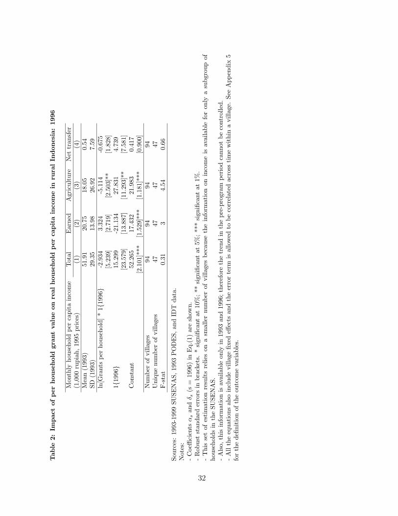
Tab

le2:

Imp

act

ofp

erh

ouse

hol

dgr

ant

valu

eon

real

hou

seh

old

per

cap

ita

inco

me

inru

ral

Ind

ones

ia:

1996

Mon

thly

hous

ehol

dpe

rca

pita

inco

me

Tot

alE

arne

dA

gric

ultu

reN

ettr

ansf

er(1

,000

rupi

ah,

1995

pric

es)

(1)

(2)

(3)

(4)

Mea

n(1

993)

51.9

120

.75

18.0

50.

54SD

(199

3)29

.35

13.9

826

.92

7.59

ln[G

rant

spe

rho

useh

old]

*1{

1996}

-2.9

343.

324

-5.1

14-0

.675

[5.2

39]

[2.7

19]

[2.5

03]*

*[1

.828

]1{

1996}

15.2

99-2

1.13

427

.831

4.73

9[2

3.57

9][1

3.88

7][1

1.29

3]**

[7.5

81]

Con

stan

t52

.265

17.4

3221

.983

0.41

7[2

.101

]***

[1.5

29]*

**[1

.181

]***

[0.9

00]

Num

ber

ofvi

llage

s94

9494

94U

niqu

enu

mbe

rof

villa

ges

4747

4747

F-s

tat

0.31

34.

540.

66

Sour

ces:

1993

-199

9SU

SEN

AS,

1993

PO

DE

S,an

dID

Tda

ta.

Not

es:

-C

oeffi

cien

tsα

san

dδ s

(s=

1996

)in

Eq.

(1)

are

show

n.-

Rob

ust

stan

dard

erro

rsin

brac

kets

.*

sign

ifica

ntat

10%

;**

sign

ifica

ntat

5%;

***

sign

ifica

ntat

1%.

-T

his

set

ofes

tim

atio

nre

sult

sre

lies

ona

smal

ler

num

ber

ofvi

llage

sbe

caus

eth

ein

form

atio

non

inco

me

isav

aila

ble

for

only

asu

bgro

upof

hous

ehol

dsin

the

SUSE

NA

S.-

Als

o,th

isin

form

atio

nis

avai

labl

eon

lyin

1993

and

1996

;th

eref

ore

the

tren

din

the

pre-

prog

ram

peri

odca

nnot

beco

ntro

lled.

-A

llth

eeq

uati

ons

also

incl

ude

villa

gefix

edeff

ects

and

the

erro

rte

rmis

allo

wed

tobe

corr

elat

edac

ross

tim

ew

ithi

na

villa

ge.

See

App

endi

x5

for

the

defin

itio

nof

the

outc

ome

vari

able

s.

32

Tab

le3:

Diff

eren

cein

the

coeffi

cien

tof

ln[G

rants

per

hou

seh

old

]*

year

du

mm

yb

etw

een

1994

and

the

sub

sequ

ent

year

sfo

rh

ouse

hol

dP

CE

(ru

ral

Ind

ones

ia):

1995

-199

9

Mon

thly

hous

ehol

dpe

rca

pita

expe

ndit

ure

Tot

alFo

odN

on-f

ood

Hou

sing

Edu

cati

onH

ealt

hC

loth

ing

Dur

able

sFe

stiv

als

(1,0

00ru

piah

,19

95pr

ices

)(1

)(2

)(3

)(4

)(5

)(6

)(7

)(8

)(1

0)M

ean

(199

3)40

.38

28.1

612

.22

5.75

0.85

0.59

1.90

1.44

1.62

SD(1

993)

14.9

210

.70

6.67

3.40

1.20

0.97

1.29

2.24

2.46

1995

-0.3

03-0

.295

-0.0

080.

125

-0.0

32-0

.091

0.03

4-0

.017

0.01

6(0

.69)

(0.5

8)(0

.98)

(0.5

6)(0

.42)

(0.0

3)(0

.63)

(0.8

5)(0

.79)

1996

-0.2

740.

023

-0.2

97-0

.15

-0.0

350.

003

0.02

60.

031

-0.1

88(0

.78)

(0.9

7)(0

.53)

(0.4

9)(0

.30)

(0.9

3)(0

.77)

(0.7

6)(0

.49)

1997

1.17

20.

577

0.59

50.

247

-0.0

01-0

.092

0.11

-0.0

490.

246

(0.1

8)(0

.36)

(0.1

3)(0

.24)

(0.9

8)(0

.20)

(0.1

3)(0

.67)

(0.0

3)

1998

0.33

3-0

.153

0.48

60.

302

-0.0

86-0

.089

0.19

1-0

.066

0.22

1(0

.79)

(0.8

7)(0

.40)

(0.3

4)(0

.09)

(0.0

8)(0

.03)

(0.6

7)(0

.06)

1999

-1.5

32-1

.980

0.44

80.

116

0.01

-0.0

390.

061

0.24

30.

048

(0.1

0)(0

.01)

(0.2

8)(0

.57)

(0.7

8)(0

.42)

(0.4

9)(0

.20)

(0.6

2)

Sour

ces:

1993

-199

9SU

SEN

AS,

1993

PO

DE

S,an

dID

Tda

ta.

Not

es:

-T

hedi

ffere

nce

inth

eco

effici

entsδ s

(s=

1995

-199

9)an

dδ 9

4(e

stim

ated

usin

gE

q.(2

))is

show

nto

geth

erw

ith

the

p-va

lue

for

the

test

ofw

heth

erth

edi

ffere

nce

isdi

ffere

ntfr

omze

ro.

-Se

eA

ppen

dix

6fo

rth

ede

finit

ion

ofth

eou

tcom

eva

riab

les.

33

Table 4 Heterogeneity in the effect of per household grant value by pre-existing village charac-teristics (rural Indonesia): 1995-1999

Outcome = Monthly household per capita Subsequent year t =expenditure (Rp.1000, 1995 prices) 1995 1996 1997 1998 1999

(1) (2) (3) (4) (5)(δs − δ94): Benchmark effect -0.972 0.674 3.911 3.632 -1.997

(0.59) (0.75) (0.12) (0.23) (0.45)(θs − θ94): Deviation from the benchmark for villages that:

Had at least one cooperative as of 1993 1.947 0.407 -2.474 -2.34 -0.545(0.29) (0.91) (0.33) (0.59) (0.86)

Received at least one public credit program in 1992 2.157 -0.482 0.681 0.581 0.653(0.33) (0.86) (0.75) (0.83) (0.79)

Were accessible via sea or air, but not land as of 1993 -1.885 4.647 6.647 10.538 -1.037(0.42) (0.10) (0.04) (0.03) (0.74)

Had at least one agriculture-related market in 1993 -2.433 0.246 1.81 -1.725 3.379(0.24) (0.94) (0.40) (0.55) (0.30)

Had at least one market facility in 1993 1.661 8.013 3.686 7.902 4.055(0.51) (0.02) (0.16) (0.14) (0.24)

Had more than the median number of households in 1993 3.876 -5.062 -6.301 -6.247 0.772(0.30) (0.23) (0.10) (0.17) (0.87)

Sources: 1993-1999 SUSENAS, 1993 PODES, and IDT data.Notes:- The difference in the coefficients δs − δ94 and θs − θ94 (s = 1995-1999) are shown together with the p-value for the test ofwhether the difference is different from zero.- Each of the estimates is obtained by estimating Eq.(3).

Table 5 Heterogeneity in the effect of per household grant value by pre-existing village charac-teristics (rural Indonesia): 1996

Outcome = Monthly household per capita Total Earned Agricultural Netincome (Rp.1000, 1995 prices) Income Income Transfer

(1) (2) (3) (4)ln[Grants per household] * 1{year = t} 37.157 17.937 -1.771 0.789

[26.460] [9.673]* [7.550] [10.878]ln[Grants per household] * 1{year = t} *

Had at least one cooperative as of 1993 11.512 9.293 13.959 -13.185[16.823] [8.249] [12.706] [8.025]

Received at least one public credit program in 1992 1.451 -2.715 2.743 1.669[2.662] [1.962] [1.438]* [1.223]

Were accessible via sea or air, but not land as of 1993 -10.549 -1.442 3.852 -8.362[14.519] [5.953] [4.143] [5.110]

Had at least one agriculture-related market in 1993 -10.963 -12.133 5.255 -5.376[11.811] [8.516] [3.891] [3.380]

Had at least one market facility in 1993 23.049 4.191 12.035 4.584[11.557]* [5.855] [5.831]** [4.812]

Had more than the median number of households in 1993 -48.368 -3.042 -17.037 -3.005[28.200]* [13.103] [8.999]* [11.071]

Number of Villages 94 94 94 94Unique number of villages 47 47 47 47F-stat 0.85 37.19 11.93 2.3

Sources: 1993-1999 SUSENAS, 1993 PODES, and IDT data.Notes:- The coefficients δ96 and θ96 are shown, where the model is Yjt = α0 +α96T96 +β96[T96 ∗Zj ] + δ96[lnFj ∗T96] + θ96[lnFj ∗T96 ∗Zj ] + µj + ujt (t = 1993 and 1996).- Robust standard errors in brackets. * significant at 10%; ** significant at 5%; *** significant at 1%.

34

Table 6 Heterogeneity in the effect of per household grant value by pre-existing village charac-teristics (rural Indonesia): 1995-1999

Outcome = Hours of work among Subsequent year t =all men aged 20-60 years 1995 1996 1997 1998 1999

(1) (2) (3) (4) (5)(δs − δ94): Benchmark effect 0.235 3.413 1.172 1.422 0.428

(0.83) (0.02) (0.50) (0.51) (0.82)(θs − θ94): Deviation from the benchmark for villages that:

Had at least one cooperative as of 1993 1.404 2.25 1.365 1.079 -0.931(0.23) (0.10) (0.39) (0.43) (0.53)

Received at least one public credit program in 1992 -2.391 -0.036 0.291 -3.331 -0.29(0.13) (0.98) (0.82) (0.02) (0.84)

Were accessible via sea or air, but not land as of 1993 -0.98 -0.792 1.98 -4.605 0.865(0.44) (0.58) (0.26) (0.02) (0.59)

Had at least one agriculture-related market in 1993 -0.768 -0.564 0.468 0.677 0.959(0.57) (0.73) (0.78) (0.70) (0.59)

Had at least one market facility in 1993 1.839 4.52 3.574 0.97 2.62(0.18) (0.00) (0.02) (0.53) (0.08)

Had more than the median number of households in 1993 3.434 -4.609 -5.528 1.139 -1.527(0.13) (0.05) (0.02) (0.68) (0.57)

Sources: 1993-1999 SUSENAS, 1993 PODES, and IDT data.Notes:- The difference in the coefficients δs − δ94 and θs − θ94 (s = 1995-1999) are shown together with the p-value for the test ofwhether the difference is different from zero.- Each of the estimates is obtained by estimating Eq.(3).

Table 7 Rate of return to per household grant value: 1995-1999

Rate of return to per household grant (%)Marginal change associated with the availability of pre-existing:

Outcome variable Overall co- public no agricultural general less-thanAverage operative credit land market market median

program access village size(1) (2) (3) (4) (5) (6) (7)

1996 PCI 26.5 119.7 22.0 -40.8 -178.6 300.7 -1089.21996 PCI in agriculture -113.9 145.1 41.6 14.9 85.6 157.0 -383.61997 PCE 1.6 -42.9 1.8 39.9 2.8 33.6 -1151997 PCE on non-food items 1.4 -6.1 13.7 19 -4.3 1.5 -34.51997 Hours of work -2.2 0.4 1.1 1.5 -0.8 2.8 -5.2

Sources: 1993-1999 SUSENAS, 1993 PODES, and IDT data.Notes:- Column 1 shows the mean of the rate of return based on the coefficients estimated using Eq.(3). Specifically, the rate is computedas (12∗ [δs +θs∗Zj ])/Fjt∗100, where δs is the coefficient of the per household grant value, θs is the coefficient of the per householdgrant value for villages that have characteristics Zj . Fjt is the grant value. I multiply the coefficient by 12 to convert monthlyPCI or PCE into an annual value. The coefficients for 1996 are used for PCI, and those for 1997 are used for PCE.- Columns 2-7 depict the change in the rate associated with the change in one of Zj , say, Zk

j from Zkj = 0 to Zk

j = 1, holding

other factors constant. That is, it is computed as: (12∗θks )/Fjt ∗100. I report this marginal change in the rate of return evaluated

at the average per household grant value among villages with Zkj = 1.

35

Appendices

Appendix 1: Infrastructure component of IDTIt is possible that the infrastructure grants given to a subset of villages increased wage employment and

enhanced investments by raising the expected returns. However, empirical results suggest that, if anything,these effects are not driving the main findings of the paper. For example, in Java, villages with lower villagescores were more likely to be selected for infrastructure grants - the value of such grants was the same acrossfunded villages (The World Bank (1995) and The World Bank (1996)). However, when villages with lowervillage scores are allowed to have differential effects of per household grant value, no significant differenceis found in the impact on PCI or PCE. In fact, only the effect on the proportion of men engaged in non-agricultural wage work is significantly larger in these villages in 1996, possibly reflecting the participation ofmen in the construction of infrastructure. In off-Java areas, villages with higher village scores were more likelyto be selected for infrastructure grants, and they were given various values of funds depending on the needsof each village (Overseas Economic Cooperation Fund (1999) and Japan Bank for International Cooperation(2001)). The value of these grants can still be correlated with the per household value of the grant for loansif villages with fewer households were more likely to receive the infrastructure grants. However, the effect onPCE does not vary by village score. Also, though the effect on PCI is stronger in those villages with highervillage scores, this income effect is driven by an increase in earned income. These results are different fromthe main findings for villages with market facilities, which is driven mainly by an increase in agriculturalincome. Thus, though there might have been a locality-specific additional effect of grants for infrastructure, itis unlikely to be the driving factor of the heterogeneity in the effect of per household value of grant for loansfor the whole of Indonesia.

Appendix 2: The rules used to select poor villages under IDT (1994-1997)In the first year, the government computed a village score based on measures of socio-economic infras-

tructure and living standards in the village. It also calculated two threshold values of the score to determinewhich villages were poor: a standard deviation (SD) indicator and a range indicator. The SD indicator isthe provincial average minus one provincial standard deviation; the range indicator is the average minus theprovincial range multiplied by 0.6. If the minimum and maximum of these two indicators are L and H anda village has a score below L, then the village is selected for a grant; if the village score is higher than H,then the village is not selected. If a score is between the two thresholds, the selection status of the villagedepends on the field officer’s evaluation. That is, if the officer thinks that the village is poor, then the villageis selected. Different sets of measures were used for urban and rural areas in computing the village score, andthus the selection of poor communities was also separately conducted (Badan Pusat Statistik (BPS) (1994)).There were few errors in this classification (Alatas (2000)).

In the second year, the government modified both the set of variables and the formula used to computethe village score. Also, neither the field officer’s subjective evaluation nor the two threshold values were usedany longer. Villages that were not funded in the first year, yet received relatively lower values for the newvillage score, were considered for funding from the second year. The number of additional poor villages wasdetermined based on the budgetary constraint. Villages that were treated in the first year were dropped if theyhad fewer than 50 families based on concern about the inequality in the per household grant value (BadanPusat Statistik (BPS) (1995)). The information on the selection rule for the third year is relatively limited.The PODES and the administrative dataset on IDT suggest that a similar rule was used to restrict very smallvillages from continued funding. In addition to her matching analysis that uses the first year rules, Alatas(2000) conducts another set of regression discontinuity analysis using the second year rules, which indicatesvarying effects for different provinces.

36

Appendix 3: Per household grant value (Rp.1000, 1995 prices)

Year Villages Mean SD1993 1811 7.0 11.41994 822 6.7 101995 499 103.7 1611996 507 154.5 1801997 509 167.9 1321998 426 145.4 1221999 469 94.3 86

Sources: 1993-1999 SUSENAS, 1993 PODES, and IDT data.Notes: The value of per household grant is defined as the cumulative value of grants received by the village divided by the numberof households as of 1993. If a village received a grant for a full three years, then the cumulative, nominal value is 20 million,40 million, and 60 million rupiah for 1995, 1996, and 1997, respectively. The nominal value remains 60 million rupiah in thepost-program period of 1998 and 1999. The value is defined as one thousand rupiah divided by the 1993 number of householdsin the pre-program period of 1993-1994. The number of villages is larger in 1993 because villages that were surveyed in 1993 andone of the later years are included for the analysis.

Appendix 4: The definition of labor supply variablesIndividualsat Work

Individuals are defined to be at work if they either (1) spent the majority of their time inthe previous week to earn income, (2) did not spend the majority of their time but spent atleast one hour to earn income, or (3) did not spend even one hour to earn income, but weretemporarily on vacation from regular work.

Agri-culturalWorkers

Individuals who are at work (workers) report the sector and occupation of the job on whichthey spend most of the time in the previous week if they fall into category (1) or (2).Individuals who fall into category (3) answer about their usual jobs. If the sector of themain job is agriculture, it includes crop cultivation, animal husbandry, forestry, fishery,hunting, and agricultural services (development of soil, rental of farming machines, andhealth services for husbandry).

Self-EmployedWorkers

These workers operate agricultural and non-agricultural businesses and bear the risk ofpossibly volatile income. They could be working on their own (e.g., vendors at markets andtrain stations) or hiring family or non-permanent, casual workers (e.g., farmers who workon their land helped by household members and vendors helped by people who are givenwages based on the days worked). Self-employed workers who hire permanent workers arecategorized as employers, who are not included in this group nor separately examined as thenumber is very small.

WageWorkers

These workers are employed by private/government institutions and receive a salary or wagesin cash or in goods. They could be permanent or casual workers and engaged in agriculturalor non-agricultural sector. Unpaid Family Workers These are not individuals who take careof household tasks such as cooking, cleaning and child-rearing; rather, these workers assisthousehold members, relatives, or neighbors, without receiving salary or wages. Examplesinclude individuals who help their parents or spouses in the fields and who help neighborsrunning a small store without receiving wages.

UnpaidFamilyWorkers

These are not individuals who take care of household tasks such as cooking, cleaning andchild-rearing; rather, these workers assist household members, relatives, or neighbors, with-out receiving salary or wages. Examples include individuals who help their parents or spousesin the fields and who help neighbors running a small store without receiving wages.

37

Appendix 5: The definition of household incomeAll these income variables include households that report no income from a specific category.

Earnedincome

Salary received from the main and side jobs, and includes fringe benefit and salary in kind.The values are in terms of 1995 prices.

Agri-culturalincome

Income accrued through the production of food and non-food crops as well as from sub-sectors such as animal husbandry, poultry, fishery, and forestry. Further disaggregateditems can be examined in the 1993 data but not in the 1996 data. In terms of 1995 prices.

Nettransfer

Inflow minus outflow of income associated with (a) gift-giving and (b) asset / financialtransactions. Gifts include grant and inheritance (inflow) and contributions and dispersedgifts (outflow). Asset transactions refer to the selling and purchasing of valuables and realestate. Financial transactions include withdrawn deposit and received loans as well as loanrepayments and making a deposit. Though IDT loans and repayments are likely to beincluded in this item, no association is found between net transfer and per household grantvalue (Column 4, Table 2). This might be an indication that transfers were not accuratelyreported. Alternatively, it might be an indication that, in smaller villages, IDT fundsare more likely to be used collectively by pokmas without being distributed to individualmembers.41 In terms of 1995 prices.

Appendix 6: Definition of household expenditureFood ex-penditure

This does not include items for household businesses, and refers only to what is consumedby household members. The values are expressed in terms of 1995 prices. Monthly foodexpenditure is defined as the expenditure in the previous week * 30 / 7.

Non-foodexpendi-ture

This also includes only items that serve for the use of household members. Monthly non-food expenditure is defined as the expenditure in the previous 12 months divided by 12. Thevalues are in terms of 1995 prices. Spending for housing includes repairs, maintenance, andutilities. Festival-related outlay includes expenses for wedding parties, religious rituals, andother celebrations. It is possible that some investments in businesses that use the residencefor production or transactions (for instance, households that sell snacks using part of theirresidence as a store) may have been counted as household expenditure.

Appendix 7: The impact on savings and livestockThe other possible form of welfare-improvement induced by IDT is increased savings. However, the 1993-

1996 change in the average amount of out-disbursement, which includes outflow of money associated with asset/ financial transactions, does not indicate any significant difference between villages with different values ofper household grants. Another possible form of savings and a source of consumption smoothing is livestock(Rosenzweig and Wolpin (1993)). However, the lack of data on livestock before the program introductionprecludes an analysis that is comparable to the analysis for employment, income and consumption outcomes.Available evidence suggests that a larger number of pigs per household was sold in villages with a largerper household grant between the beginning of 1997 (the last year of the program period) and that of 1998(Appendix Table 3). No significant difference is found in the pattern of transactions of cows, buffalos, horses,goats, sheep, chickens and ducks. It is possible that pigs were purchased during the program period, andthen sold later during the currency crisis (between January of 1997 and January of 1998) to shelter householdexpenditure from a possible loss in income. However, the pattern of transactions during the program periodcannot be tested. Also, without the knowledge of whether and how much the size of the income loss thatwould have been realized without any response differed between small and large villages, it is difficult to assesswhether the loss is associated with the sales of pigs.

38

Appendix 8[A]: Definition and summary statistics for village characteristicsAvailabilityof sourcesof creditother thanIDT

Two dummy variables are used. One indicates a village where at least one cooperative wasoperating as of 1993; the other indicates a village that received some public credit programsin 1992. Public credit programs include Farmers Enterprise Credit, Community Sugar CaneIntensification Credit (TRI), Candak kulak credit, and other credit provided by foundationswith a legal status. These do not include usurers.

General/ agri-culturalmarketfacility

Two dummy variables are used indicating a village that had at least one general-purposemarket facility and at least one facility related to agricultural production. A general-purposemarket includes a permanent or semi permanent building that is used as a market, a non-permanent building made of materials such as bamboo and leaves, and a group of at least10 shops. An agriculture-related market facility includes a production tools kiosk whereagricultural inputs such as fertilizer and seedlings are sold, warehouses where agriculturalproducts are stored, and a fish market.

Trans-portation/ access

A dummy variable indicating a village with no land access is used.

Villagesize

A dummy variable is included indicating a village where the number of households as of1993 was greater than the median.

Other vil-lage char-acteristics

The following pre-existing characteristics have been tested for a possible heterogeneous ef-fect of the program; however, they do not show any evidence for heterogeneity, thus arenot included. The first is the characteristics of the village head, that is, whether the villagehead was older than the median age and whether the head completed secondary education.The second is the educational attainment of the population, as measured by the propor-tion of adults aged 20-60 who completed secondary education and the gender gap in theproportion. Third, the existence of a bank (one type of credit sources) does not show sys-tematic evidence for heterogeneity in the program effects. Fourth, additional informationon road conditions does not indicate heterogeneous effects such as dummy variables distin-guishing, among villages with land access, places where inter-village roads are hardened,places where inter-village roads are made of asphalt, and places where inter-village roadsare soil or pebbles.

Appendix 8[B]: Summary statistics for the village characteristics included in the analysis

Village Characteristics Mean SD1{Village had at least one cooperative as of 1993} 0.108 0.3111{Village received at least one public credit program in 1992} 0.360 0.4801{Village was accessible via sea or air as of 1993} 0.130 0.3371{Village had at least one market facility as of 1993} 0.149 0.3561{Village had at least one agriculture-related market as of 1993} 0.260 0.4391{Village size was less than the median as of 1993} 0.506 0.500Number of villages 1811

Sources: 1993 SUSENAS, 1993 PODES, and IDT data.

39