Journal of Immunological Methods 316 (2006) 52–58www.elsevier.com/locate/jim

Research paper

The automated counting of spots for the ELISpot assay

Natalie Hawkins ⁎, Steve Self, Jon Wakefield

Fred Hutchinson Cancer Research Center, Statistical Center for HIV Aids Research and Prevention, 1100 Fairview Avenue, LE-400,Seattle, WA 98109, United States

Received 15 March 2006; received in revised form 23 June 2006; accepted 10 August 2006Available online 12 September 2006

Abstract

An automated method for counting spot-forming units in the ELISpot assay is described that uses a statistical model fit totraining data that is based on counts from one or more experts. The method adapts to variable background intensities and providesconsiderable flexibility with respect to what image features can be used to model expert counts. Point estimates of spot counts areproduced together with intervals that reflect the degree of uncertainty in the count. Finally, the approach is completely transparentand “open source” in contrast to methods embedded in current commercial software. An illustrative application to data from a studyof the reactivity of T-cells from healthy human subjects to a pool of immunodominant peptides from CMV, EBV and flu ispresented.© 2006 Elsevier B.V. All rights reserved.

Keywords: Automated spot counting; ELISpot assay; Image analysis; Generalized linear models

1. Introduction

T-lymphocyte response to vaccination represents theprimary immunogenicity endpoint in Phase I/II trials ofcurrent candidate HIV vaccines (Koup et al., 1994;Borrow et al., 1994; Rowland-Jones et al., 1995; Mazzoliet al., 1997;Musey et al., 1997;Ogg et al., 1998;Goh et al.,1999), and the use of a highly standardized, sensitive assayto measure these responses is a critical requirement in thedevelopment and evaluation ofHIV vaccines. The ELISA-spot or ELISpot assay currently represents the primary

Abbreviations: CMV, cytomegalovirus; EBV, Epstein–Barr virus;ELISpot, enzyme-linked immunospot; HIV, human immunodeficiencyvirus; T-cell, T-lymphocyte; SFU, spot-forming unit; TIFF, TaggedImage File Format.⁎ Corresponding author. Tel.: +1 206 667 7753; fax: +1 206 667

4812.E-mail address: hawkins@scharp.org (N. Hawkins).

0022-1759/$ - see front matter © 2006 Elsevier B.V. All rights reserved.doi:10.1016/j.jim.2006.08.005

method to detect T-cell responses to HIV vaccines in theHIVVaccine Trials Network. Considerable effort has beenmade to standardize the reagents and laboratory proce-dures used in these assays. However methods for thecounting of spot-forming units (SFUs), which is used toobtain the final quantitative result of the ELISpot assay,have received somewhat less attention.

Historically, SFUs have been hand-counted bylaboratory technicians but such subjective readingsintroduce significant variability in the assay outcomeand are time-consuming. Computer algorithms for theanalysis of images of the wells have been employed toautomate the process of spot counting (Hudgens et al.,2004). Although automated spot counting algorithms canprovide highly standardized assay outcomes, there arechallenges to this approach that call into question theultimate accuracy of these methods. Specifically, there isno “gold standard” for defining an SFU that can explicitly

53N. Hawkins et al. / Journal of Immunological Methods 316 (2006) 52–58

be used in algorithm design. In addition, such algorithmsmust integrate an automated method for calibration tobackground intensity levels that vary from plate to plateand distinguish “true SFUs” from various artifacts thatinclude variable background intensity within wells (e.g.,edge effects) and contamination. Examples of imagesfrom ELISpot assays that illustrate some aspects of thisvariability are given in Fig. 1. Numbering from left toright and top to bottom, wells 1, 4 and 5 contain clearartifacts, while there are dark patches close to the edges ofa number of wells.

In this work, we propose an automated approach tothe analysis of images from ELISpot assays that

Fig. 1. Nine typical wells, showing spot

provides accurate and highly standardized counts ofSFUs. In the absence of a gold standard for defining anSFU, we define the conceptual criterion of success forthe method as a standardized implementation of theimplicit rules for use by a designated expert (or possiblya panel of such experts) in counting SFUs. Specifically,the method uses “training data”, composed of SFUcounts by an expert, in order to refine the algorithm toproduce counts that are accurate reflections of the expertcounts but, unlike counts by any human, are uniformlyapplied from assay to assay. The model-based approachwe describe allows the uncertainty in the count to beacknowledged, so that an interval estimate for the

forming units and various artifacts.

54 N. Hawkins et al. / Journal of Immunological Methods 316 (2006) 52–58

number of spots per well is produced. The method isillustrated using data from a study of the reactivity of T-cells from healthy human subjects to a pool ofimmunodominant peptides from CMV, EBV and flu.

2. Methods

In this section we describe the method of assigning aspot count to each well, along with an associatedinterval estimate. The method has two components.First, we pre-process the image using a thresholding andgrouping technique to identify interesting areas whichwe call “globs”. Second, based on training data, weformulate a model to predict the number of spots in eachglob, based on glob characteristics such as the size of theglob. The resulting model is used to predict the numberof spots in a new well, along with an interval estimate.

2.1. Pre-processing

For each well, the raw data originate from a TaggedImage File Format (TIFF) file and consist of pixel-levelred, green and blue intensities, displayed in Fig. 1. Forprocessing we use grey scale values by computing amean of the red, green, and blue values to get an inten-sity at each pixel. These values range from 0 to 255 andare such that high intensities correspond to background,while low intensities correspond to spots, and toanomalies of the measurement process, such as anerrant hair in the well.

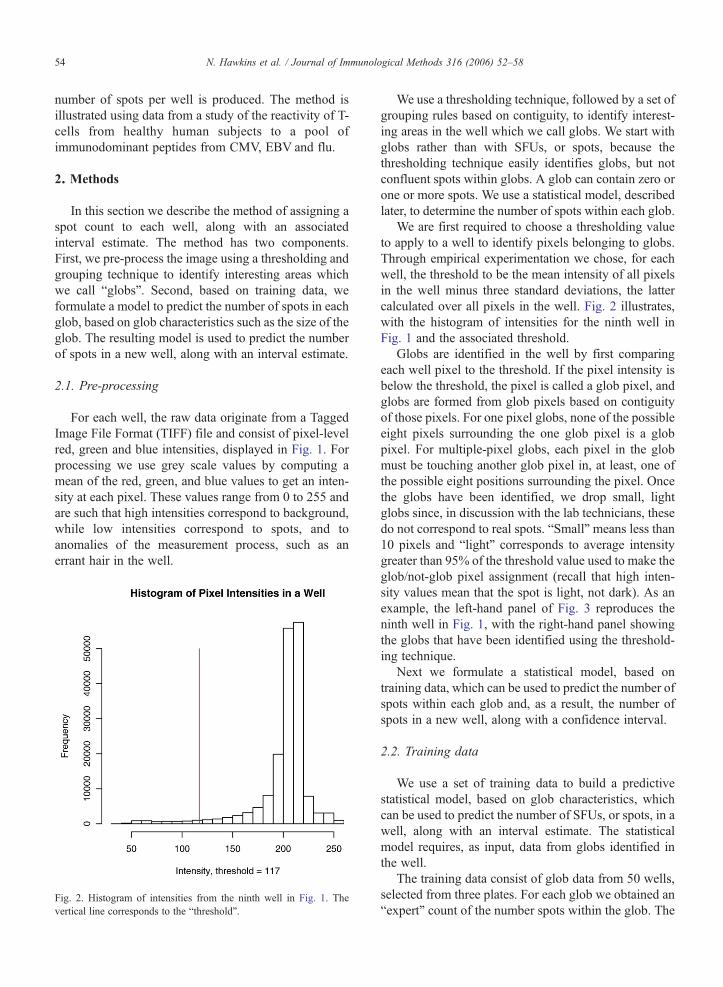
Fig. 2. Histogram of intensities from the ninth well in Fig. 1. Thevertical line corresponds to the “threshold”.

We use a thresholding technique, followed by a set ofgrouping rules based on contiguity, to identify interest-ing areas in the well which we call globs. We start withglobs rather than with SFUs, or spots, because thethresholding technique easily identifies globs, but notconfluent spots within globs. A glob can contain zero orone or more spots. We use a statistical model, describedlater, to determine the number of spots within each glob.

We are first required to choose a thresholding valueto apply to a well to identify pixels belonging to globs.Through empirical experimentation we chose, for eachwell, the threshold to be the mean intensity of all pixelsin the well minus three standard deviations, the lattercalculated over all pixels in the well. Fig. 2 illustrates,with the histogram of intensities for the ninth well inFig. 1 and the associated threshold.

Globs are identified in the well by first comparingeach well pixel to the threshold. If the pixel intensity isbelow the threshold, the pixel is called a glob pixel, andglobs are formed from glob pixels based on contiguityof those pixels. For one pixel globs, none of the possibleeight pixels surrounding the one glob pixel is a globpixel. For multiple-pixel globs, each pixel in the globmust be touching another glob pixel in, at least, one ofthe possible eight positions surrounding the pixel. Oncethe globs have been identified, we drop small, lightglobs since, in discussion with the lab technicians, thesedo not correspond to real spots. “Small” means less than10 pixels and “light” corresponds to average intensitygreater than 95% of the threshold value used to make theglob/not-glob pixel assignment (recall that high inten-sity values mean that the spot is light, not dark). As anexample, the left-hand panel of Fig. 3 reproduces theninth well in Fig. 1, with the right-hand panel showingthe globs that have been identified using the threshold-ing technique.

Next we formulate a statistical model, based ontraining data, which can be used to predict the number ofspots within each glob and, as a result, the number ofspots in a new well, along with a confidence interval.

2.2. Training data

We use a set of training data to build a predictivestatistical model, based on glob characteristics, whichcan be used to predict the number of SFUs, or spots, in awell, along with an interval estimate. The statisticalmodel requires, as input, data from globs identified inthe well.

The training data consist of glob data from 50 wells,selected from three plates. For each glob we obtained an“expert” count of the number spots within the glob. The

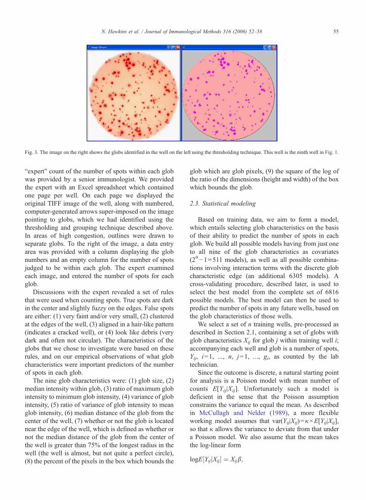
Fig. 3. The image on the right shows the globs identified in the well on the left using the thresholding technique. This well is the ninth well in Fig. 1.

55N. Hawkins et al. / Journal of Immunological Methods 316 (2006) 52–58

“expert” count of the number of spots within each globwas provided by a senior immunologist. We providedthe expert with an Excel spreadsheet which containedone page per well. On each page we displayed theoriginal TIFF image of the well, along with numbered,computer-generated arrows super-imposed on the imagepointing to globs, which we had identified using thethresholding and grouping technique described above.In areas of high congestion, outlines were drawn toseparate globs. To the right of the image, a data entryarea was provided with a column displaying the globnumbers and an empty column for the number of spotsjudged to be within each glob. The expert examinedeach image, and entered the number of spots for eachglob.

Discussions with the expert revealed a set of rulesthat were used when counting spots. True spots are darkin the center and slightly fuzzy on the edges. False spotsare either: (1) very faint and/or very small, (2) clusteredat the edges of the well, (3) aligned in a hair-like pattern(indicates a cracked well), or (4) look like debris (verydark and often not circular). The characteristics of theglobs that we chose to investigate were based on theserules, and on our empirical observations of what globcharacteristics were important predictors of the numberof spots in each glob.

The nine glob characteristics were: (1) glob size, (2)median intensity within glob, (3) ratio of maximum globintensity to minimum glob intensity, (4) variance of globintensity, (5) ratio of variance of glob intensity to meanglob intensity, (6) median distance of the glob from thecenter of the well, (7) whether or not the glob is locatednear the edge of the well, which is defined as whether ornot the median distance of the glob from the center ofthe well is greater than 75% of the longest radius in thewell (the well is almost, but not quite a perfect circle),(8) the percent of the pixels in the box which bounds the

glob which are glob pixels, (9) the square of the log ofthe ratio of the dimensions (height and width) of the boxwhich bounds the glob.

2.3. Statistical modeling

Based on training data, we aim to form a model,which entails selecting glob characteristics on the basisof their ability to predict the number of spots in eachglob. We build all possible models having from just oneto all nine of the glob characteristics as covariates(29−1=511 models), as well as all possible combina-tions involving interaction terms with the discrete globcharacteristic edge (an additional 6305 models). Across-validating procedure, described later, is used toselect the best model from the complete set of 6816possible models. The best model can then be used topredict the number of spots in any future wells, based onthe glob characteristics of those wells.

We select a set of n training wells, pre-processed asdescribed in Section 2.1, containing a set of globs withglob characteristics Xij for glob j within training well i;accompanying each well and glob is a number of spots,Yij, i=1, ..., n, j=1, …, gi, as counted by the labtechnician.

Since the outcome is discrete, a natural starting pointfor analysis is a Poisson model with mean number ofcounts E[Yij|Xij]. Unfortunately such a model isdeficient in the sense that the Poisson assumptionconstrains the variance to equal the mean. As describedin McCullagh and Nelder (1989), a more flexibleworking model assumes that var(Yij|Xij)=κ×E[Yij|Xij],so that κ allows the variance to deviate from that undera Poisson model. We also assume that the mean takesthe log-linear form

logE½YijjXij� ¼ Xijb;

Table 1Summary of parameter estimates from best-fitting model

Characteristic Estimate Standarderror

p-value

Located near edge 1.20 0.859 0.164Height–width ratio −0.0901 0.3186 0.7775Median intensity in glob −0.0325 0.00362 2.0×10−16

Variance of intensities in glob 0.00447 0.000427 2.0×10−16

Ratio of variance to meanintensities in glob

−0.606 0.0608 2.0×10−16

Glob size 0.000105 0.000313 0.737Median distance of glob fromthe center of the well

−0.000308 0.000955 0.747

Ratio of max to min intensityin glob

0.279 0.0867 0.00135

Edge×height–width ratio −1.74 0.634 0.00620Edge×size 0.000418 0.000532 0.433Edge×median distance fromcenter of well

−0.00560 0.00420 0.183

Fig. 4. Number of spots as predicted by the model-based approach andthe current automated lab method, for 50 wells.

56 N. Hawkins et al. / Journal of Immunological Methods 316 (2006) 52–58

though our method could use any form. For example,the method we describe could be applied to anyparametric or semi-parametric model including logicregression, generalized additive models, or splines, seeHastie, Tibshirani, and Friedman (2000) for more detailon these methods. A quasi-likelihood method ofinference, as described in McCullagh and Nelder(1989), is used to estimate the parameters of themodel; this method has the advantage of requiring thespecification of the first two moments of the data,without making a distributional assumption. Themethod we describe can also be used with specificdistributional assumptions, if these appear reasonable inany particular application. We also use sandwichestimation (Royall, 1986) to provide empirical esti-mates of the standard errors. This approach provides aconsistent estimator of the standard errors, givenindependent glob counts.

The over-dispersion parameter, along with sandwichestimation, is designed to account for components ofvariation that are attributed to well and/or plate.Although there are methods for improving predictionerror of counts for one well using data from other wellson the same plate, in our experience working withlaboratory scientists, they prefer to make prediction foreach well independently. We wish to have a generalmethod and not one which needs retuning in eachdifferent scenario.

Once we have selected the best predictive model ofthe type described above, based on the training data, themodel can be used to predict the number of spots in anew well. Let Xj denote the glob characteristics of a newwell containing j=1, …, nnew, globs, for which werequire an estimate of the number of spots, call this θ.

Once estimates β and κ are obtained, a prediction isavailable via h ¼ Pnnew

j¼1 expðXjbÞ, which is an unbiasedestimate.

Using the delta method to obtain the variance of θ,we obtain an approximate 95% interval for the totalnumber of spots that is given by:

Xnnewj¼1

expðXjbÞF 1:96

�Xnnewj¼1

expðXjbÞXj

( )V

Xnnewj¼1

XTj expðXjbÞ

( )" #1=2

where V is the sandwich estimate of the variance of β.

3. Results

We wish to use the training data to decide on whichof the 9 glob characteristics are important predictors ofthe number of spots that each glob contains, in order tofind the model which would best serve as a predictivemodel. Specifically we have a total of K=6816 models,this set consisting of all possible models containing ornot-containing each of the 9 glob characteristics, as wellas all possible interaction models containing aninteraction with the discrete glob characteristic, edge.We use a cross-validation technique, in which we use 49of the training wells to estimate the parameters of model,Mk , k=1, …, K, and then predict the number of spots in

57N. Hawkins et al. / Journal of Immunological Methods 316 (2006) 52–58

the 50th well; repeating this procedure and leaving out adifferent well each time, gives a set of predictions Ŷijk

under model k, so that we can calculate the modelassessment sum of squares criteria

SSk ¼Xni¼1

Xgij¼1

ðYij−YijkÞ2;

k=1, …, K . After training the model with data fromglobs from 50 wells, we found the best model, based onthe minimum SSk.

The best model was found to contain eight globcharacteristics and three interaction terms with the globcharacteristic edge: (1) edge, (2) height–width ratio,defined as the square of the log of the ratio of thedimensions (height and width) of the box which boundsthe glob, (3) median intensity, (4) variance of theintensity, (5) variance of the intensity divided by themean intensity, (6) size, (7) median distance from thecenter of the well, (8) the ratio of the maximum intensityto the minimum intensity; and interactions of edge with:(1) height–width ratio, (2) size, and (3) median distancefrom the center of the well. Once we have decided uponthis model we re-estimate the coefficients based on all50 wells. Table 1 contains the resulting estimates, alongwith their standard errors.

From the coefficients we see that globs classified asnear the edge are more likely to contain more spots. Themore rectangular the glob is, as measured by the height–width ratio, the less likely it is to contain more spots.Darker globs (as measured by lower median intensity)are more likely to contain more spots, while moreconstant intensity within a glob implies fewer spots. Asthe ratio of the variance of the intensity to the meanintensity increases the number of spots decreases. Globscontaining more pixels are more likely to contain morespots. Globs that are located further from the center ofthe well are more likely to contain fewer spots(reflecting the anomalies that occur towards the outsideof the well, see Fig. 1, wells 4 and 6 in particular).Finally, greater maximum to minimum intensitiessuggest more spots also. Looking at the interactionterms we see that globs near the edge and morerectangular (as measured by the height–width ratio) arelikely to contain fewer spots. Larger globs near the edgeare more likely to contain more spots, and globsclassified as near the edge but which are closer to theedge are likely to contain fewer spots. The non-significance of four of the variables and two of theinteraction terms, is perhaps surprising but it is thecombination of variables that is important from aprediction point of view.

Fig. 4 shows the estimated number of spots in each ofthe 50 wells from our method, versus those from thelaboratory expert. Also shown are the estimates from theautomated method currently used by the lab. For clarity,for a small collection of wells we include our confidenceinterval, based on the sandwich estimator of thevariance. For plotting, we have jittered the values onthe x-axis slightly to uncover points which might beoverlapping so that all 100 points are visible on the plot.We see that the model predictions are more accuraterelative to the expert technician, than is the commercialsoftware being used by the lab. As confirmation ofthis we can evaluate the average bias, given by1=n

Pni¼1ðYi−Y iÞ, and the mean squared error (MSE),

given by 1=nPn

i¼1ðYi−Y iÞ2, where Yi and Ŷi are theobserved and predicted number of spots in well i, foreach of the model-based and current automated labmethods. For the model-based approach we obtain anaverage bias and MSE of 0.0336 and 5.68, while forthe current automated lab method we obtained averagebias and MSE of 3.49 and 26.4. Hence we see themodel-based approach provides more accurate pre-dicted numbers of spots, as measured by both bias andprecision; in particular the commercial softwareprovides an overcount of the number of spots.

4. Discussion

There is no “gold standard” method of spot countingto which automated methods can be compared. In theabsence of such a standard, expert opinion with all of itsassociated vagaries, represents the standard by whichautomated methods must be judged. However expertopinion must first be operationally defined. We haveoperationally defined expert opinion in this work as thecounts made on our training data set by a seniorimmunologist with whom we have collaborated. Thishas served our purpose of providing a realistic andpertinent illustration of a specific application of ourproposed method. A broader definition based on a panelof immunologists might also have been used. We leaveto future work the development of a more extensive setof training data together with an associated consensusexpert opinion of spot counts that might provide a moredefinitive and broadly applicable counting algorithmbased on our methods.

The accuracy of an automated counting method refersto how faithfully the method replicates the counts fromexpert opinion on average (over globs). Our proposedmethod is trained directly from expert opinion usingstatistical methods that guarantee (in large samples) suchaccuracy. We expect that this will provide a more

58 N. Hawkins et al. / Journal of Immunological Methods 316 (2006) 52–58

accurate reproduction of counts based on expert opinionthan other methods that are indirectly “calibrated”.

Assessing the precision of automated methods ischallenging because there is innate non-systematicvariability in expert opinion. This variability is reflectedin the fact that expert recounts do not always result inexactly the same number of spots per well. Thiscomponent of random variation will be inherited byany automated method. The proposed counting methodis based on measurable characteristics of globs and, tothe extent that these characteristics capture all factorsconsidered systematically by experts in their counts, theautomated methods will faithfully replicate the expertopinion up to the aforementioned random variability.We expect that a certain amount of systematic variationin expert counts will not be captured by readilymeasurable glob characteristics so that automatedmethods will inevitably be somewhat more variablethan the theoretical minimum variation defined byrecount variability. However, the proposed method iscompletely flexible with respect to the set of measurableglob characteristics that can be considered as possiblepredictors with practical limits on this set imposed onlyby the size of the training data set. Thus, with anextensive training data set and careful elicitation of theglob characteristics and other factors considered byexperts in performing their counts, it is reasonable toexpect that the proposed method will reproduce thesystematic variation in expert counts.

One advantage of the proposed method is thatinterval estimates of spot counts are naturally producedthat reflect the degree of uncertainty in the count. Thisinterval estimate can be used as a component of theassay quality control process to reflect reliability ofcounts delivered for each well. The estimated variabilityin spot count at the well level can also form the basis fora similar estimate of variability for summary measuresof response that combine spot counts over multiplewells (e.g. total response across peptide-treated wells netof response in negative control wells).

Finally, the proposed method provides a completelytransparent “open-source” approach for spot countingthat is in contrast to proprietary methods embedded incommercial software that often function as a black-box.In the current atmosphere that places considerable value

on standardization of reagents and operating proceduresfor immunologic assays used in the development andevaluation of HIV vaccines (Klausner et al., 2003), theproposed method represents a natural approach toextending this standardization to the final critical stepof the assay process.

References

Borrow, P., Lewicki, H., Hahn, B.H., Shaw, G.M., Oldstone, M.B.,1994. Virus-specific CD8-cytotoxic T-lymphocyte activity associ-ated with control of viremia in primary human immunodeficiencyvirus type 1 infection. Journal of Virology 68, 6103.

Goh, W.C., Markee, J., Akridge, R.E., et al., 1999. Protection againsthuman immunodeficiency virus type 1 infection in persons withrepeated exposure: evidence for T cell immunity in the absence ofinherited CCR5 coreceptor defects. Journal of Infectious Diseases179, 548.

Hastie, T., Tibshirani, R., Friedman, J., 2000. The Elements ofStatistical Learning, Data Mining, Inference and Prediction.Springer, Verlag.

Hudgens, M., Self, S., Chiu, Ya-Lin, et al., 2004. Statisticalconsiderations for the design and analysis of the ELISpot assayin HIV-1 vaccine trials. Journal of Immunological Methods 288,19.

Klausner, R.D., Fauci, A.S., Corey, L., 2003. The need for a globalHIV vaccine enterprise. Science 300, 2036.

Koup, R.A., Safrit, J.T., Cao, Y., Andrews, C.A., McLeod, G.,Borkowsky, W., Farthing, C., Ho, D.D., 1994. Temporal associationof cellular immune responses with the initial control of viremia inprimary human immunodeficiency virus type 1 syndrome. Journal ofVirology 68, 4650.

Mazzoli, S., Trabattoni, D., Lo Caputo, S., et al., 1997. HIV-specificmucosal and cellular immunity in HIV-seronegative partners ofHIV-seropositive individuals. Nature Medicine 3, 1250.

McCullagh, P., Nelder, J.A., 1989. Generalized Linear Models, Secondedition. Chapman and Hall.

Musey, L., Hughes, J., Schacker, T., Shea, T., Corey, L., McElrath, M.J.,1997. Cytotoxic-T-cell responses, viral load, and disease progressionin early human immunodeficiency virus type 1 infection. NewEngland Journal of Medicine 337, 1267.

Ogg, G.S., Jin, X., Bonhoeffer, S., Dunbar, P.R., Nowak, M.A.,Monard, S., Segal, J.P., Cao, Y., Rowland-Jones, S.L., Cerundolo,V., Hurley, A., Markowitz, M., Ho, D.D., Nixon, D.F., McMichael,A.J., 1998. Quantitation of HIV-1-specific cytotoxic T lympho-cytes and plasma load of viral RNA. Science 279, 2103.

Rowland-Jones, S., Suttone, J., Ariyoshi, K., et al., 1995. HIV-specificcytotoxic T-cells in HIV-exposed but uninfected Gambian women.Nature Medicine 1, 59.

Royall, R., 1986. Model robust confidence intervals using maximumlikelihood estimators. International Statistical Review 54, 221.