the battelle integrity of - nrc: home page · the battelle integrity of nuclear piping (binp)...

NUREG/CR-6837, Vol. 2

The Battelle Integrity of Nuclear Piping (BINP) Program Final Report

Appendices

U.S. Nuclear Regulatory CommissionOffice of Nuclear Regulatory ResearchWashington, DC 20555-0001

NUREG/CR-6837, Vol. 2

The Battelle Integrity ofNuclear Piping (BINP)Program Final Report

AppendicesManuscript Completed: September 2003Date Published: June 2005

Prepared byP.Scott1, R.Olson1, J.Bockbrader1, M.Wilson1, B.Gruen1,R.Morbitzer1, Y.Yang1, C.Williams1, F.Brust1, L.Fredette1,N.Ghadiali1

G.Wilkowski2, D.Rudland2, Z.Feng2, R.Wolterman2

. 1Battelle505 King AvenueColumbus, OH 43201

Subcontractor:2Engineering Mechanics Corporation of Columbus3518 Riverside DriveSuite 202Columbus, OH 43221-1735

C. Greene, NRC Project Manager

Prepared forDivision of Engineering TechnologyOffice of Nuclear Regulatory ResearchU.S. Nuclear Regulatory CommissionWashington, DC 20555-0001NRC Job Code W6775

DISCLAIMER: This report was prepared as an account of work sponsored by an agency of the U.S. Government. Neither the U.S. Government nor any agency thereof, nor any employee, makes any warranty, expressed orimplied, or assumes any legal liability or responsibility for any third party’s use, or the results of such use, of anyinformation, apparatus, product, or process disclosed in this publication, or represents that its use by such thirdparty would not infringe privately owned rights.

AVAILABILITY OF REFERENCE MATERIALS

IN NRC PUBLICATIONS

NRC Reference Material

As of November 1999, you may electronically accessNUREG-series publications and other NRC records atNRC’s Public Electronic Reading Room at http://www.nrc.gov/reading-rm.html. Publicly releasedrecords include, to name a few, NUREG-seriespublications; Federal Register notices; applicant,licensee, and vendor documents and correspondence;NRC correspondence and internal memoranda;bulletins and information notices; inspection andinvestigative reports; licensee event reports; andCommission papers and their attachments.

NRC publications in the NUREG series, NRCregulations, and Title 10, Energy, in the Code ofFederal Regulations may also be purchased from oneof these two sources.1. The Superintendent of Documents U.S. Government Printing Office Mail Stop SSOP Washington, DC 20402–0001 Internet: bookstore.gpo.gov Telephone: 202-512-1800 Fax: 202-512-22502. The National Technical Information Service Springfield, VA 22161–0002 www.ntis.gov 1–800–553–6847 or, locally, 703–605–6000

A single copy of each NRC draft report for comment isavailable free, to the extent of supply, upon writtenrequest as follows:Address: Office of the Chief Information Officer, Reproduction and Distribution Services Section U.S. Nuclear Regulatory Commission Washington, DC 20555-0001E-mail: [email protected] Facsimile: 301–415–2289

Some publications in the NUREG series that are posted at NRC’s Web site addresshttp://www.nrc.gov/reading-rm/doc-collections/nuregs are updated periodically and may differ from the lastprinted version. Although references to material foundon a Web site bear the date the material wasaccessed, the material available on the date cited maysubsequently be removed from the site.

Non-NRC Reference Material

Documents available from public and special technicallibraries include all open literature items, such asbooks, journal articles, and transactions, FederalRegister notices, Federal and State legislation, andcongressional reports. Such documents as theses,dissertations, foreign reports and translations, andnon-NRC conference proceedings may be purchasedfrom their sponsoring organization.

Copies of industry codes and standards used in asubstantive manner in the NRC regulatory process aremaintained at—

The NRC Technical Library Two White Flint North11545 Rockville PikeRockville, MD 20852–2738

These standards are available in the library for reference use by the public. Codes and standards areusually copyrighted and may be purchased from theoriginating organization or, if they are AmericanNational Standards, from—

American National Standards Institute11 West 42nd StreetNew York, NY 10036–8002www.ansi.org 212–642–4900

Legally binding regulatory requirements are statedonly in laws; NRC regulations; licenses, includingtechnical specifications; or orders, not in NUREG-series publications. The views expressedin contractor-prepared publications in this seriesare not necessarily those of the NRC.

The NUREG series comprises (1) technical andadministrative reports and books prepared by thestaff or agency contractors, (2) proceedings ofconferences, (3) reports resulting from internationalagreements, (4) brochures, and (5) compilations oflegal decisions and orders of the Commission andAtomic and Safety Licensing Boards and ofDirectors’ decisions under Section 2.206 of NRC’sregulations (NUREG–0750).

http://www.nrc.gov/reading-rm.html.

http://www.nrc.gov/reading-rm/doc-collections/nuregs

iii

ABSTRACT

Volume I of the final report for the Battelle Integrity of Nuclear Piping (BINP) program provided a summary of the results from this program and a discussion of the implications of those results. This volume (Volume II - Appendices) provides the details from

the various technical tasks conducted as part of this program. Each individual appendix provides the details of a specific task conducted as part of the BINP program.

v

FOREWORD

Since 1965, the U.S. Nuclear Regulatory Commission (NRC) has been involved in research on various aspects of pipe fracture in nuclear power plant piping systems. The most recent programs are the Degraded Piping Program, Short Cracks in Piping and Piping Welds Program, and two International Piping Integrity Research Group programs. These programs have developed and validated “state-of-the-art” structural analysis methods and data for nuclear piping systems. This report describes the results of the Battelle Integrity of Nuclear Piping (BINP) program, which was performed by Battelle Columbus Laboratories. The objective of the BINP program was to address the most important unresolved technical issues from the earlier research programs. The BINP program was initiated as an international program to enable fiscal leveraging and an expanded scope of work. Technical direction for the program was provided by a Technical Advisory Group composed of representatives from the funding organizations. The BINP program was divided into eight independent tasks, each of which examined one of the unresolved technical issues. These eight tasks included both experimental and analytical efforts. The two pipe-system experiments examined the effects of secondary stresses (such as thermal expansion) and cyclic loading (such

as during a seismic event) on the load-carrying capacity of flawed piping. For these experiments, the pipe system had large flaws or cracks. The remaining six tasks were “best-estimate” analyses to examine the effects of other factors, such as pipe system boundary conditions, and weld residual stresses on the behavior of flawed pipes. Many of these analyses involved the use of finite element modeling techniques. One of these analytical tasks was to examine the actual margins that may exist in flawed pipe evaluations as a result of non-linear behavior. While the magnitude of these margins would vary on a case-by-case basis, the results of this task show that a potential for significant margins does exist. In addition to developing a technical basis for more advanced inservice flaw evaluation procedures for use with Class 1 piping, as defined by the American Society of Mechanical Engineers (ASME), the BINP program considered the development of flaw evaluation procedures for ASME Class 2 and 3 piping and balance-of-plant piping. This research supports the NRC’s goal to improve the effectiveness and realism of the agency’s regulatory actions. Carl Paperiello, Director Office of Nuclear Regulatory Research U.S. Nuclear Regulatory Commission

vii

Table of Contents

Abstract………………………………………………………………………………………….iii

Foreword………………………………………………………………………………………..v

Appendix A Evaluation of Procedures for the Treatment of Secondary Stresses in Pipe Fracture Analyses…………………………………………………………………………………....A1

Appendix B Pipe-System Experiment with an Alternative Simulated Seismic Load History...................................................................................................................................B1

Appendix C BINP Task 3 – Determination of Actual Margins in Plant Piping………………..C1

Appendix D Analytical Expressions Incorporating Restraint of Pressure-Induced Bending in Crack-Opening Displacement Calculations………………………………………………..D1

Appendix E Development of Flaw Evaluation Criteria for Class 2, 3, and Balance of Plant Piping……………………………………………………………………………………….E1

Appendix F The Development of a J-Estimation Scheme for Circumferential and Axial Through-Wall Cracked Elbows………………………………………………………………………………………F1

Appendix G Evaluation of Reactor Pressure Vessel (RPV) Nozzle to Hot-Leg Piping Bimetallic Weld Joint Integrity for the V. C. Summer Nuclear Power Plant………………………….G1

Appendix H The Effect of Weld Induced Residual Stresses on Pipe Crack Opening Areas and Implications on Leak-Before-Break Considerations……………………………………….H1

Appendix I Round Robin Analyses……………………………………………………………...I1

List of Figures

Figure A.1 Comparison of the results from the IPIRG-1 pipe-system experiments with companion quasi-static, four-point bend experiments demonstrating how global secondary stresses, such as thermal expansion and seismic anchor motion stresses, contribute to fracture.................................................................................................................................. A2

Figure A.2 Actuator time history for BINP Task 1 experiment and IPIRG-1 Experiment 1.3-5 .................................................................................................................. A3

Figure A.3 Plot of crack section moment as function of time for BINP Task 1 experiment and IPIRG-1 Experiment 1.3-5 ................................................................................................... A4

Figure A.4 Comparison of the results from four stainless steel weld experiments showing the contributions of the various stress components to pipe fracture ...................... A4

viii

Figure B.1 Actuator displacement-time history for IPIRG-2 simulated seismic forcing function for stainless steel base metal experiment (Experiment 1-1) ..................................................B2

Figure B.2 Moment-rotation response for IPIRG-2 simulated seismic forcing function for stainless steel base metal experiment (Experiment 1-1)........................................................B2

Figure B.3 Traditional seismic design process ............................................................................B4

Figure B.4 Hypothesized worst case seismic loading..................................................................B6

Figure B.5 Typical SSE seismic floor-response spectra..............................................................B6

Figure B.6 Fracture toughness properties from pipe DP2-A8i ....................................................B7

Figure B.7 Fracture toughness properties from pipe DP2-A8ii...................................................B7

Figure B.8 Spring-slider model for a surface crack.....................................................................B8

Figure B.9 Kinematic hardening assumption under unloading conditions..................................B9

Figure B.10 The effect of pressure on crack moment-rotation behavior (BINP Task 2 flaw, A8ii-20 dynamic monotonic J-resistance).............................................................................B9

Figure B.11 Crack unloading behavior......................................................................................B10

Figure B.12 IPIRG-2 Experiment 1-1 cracked-section moment-rotation response...................B12

Figure B.13 IPIRG-2 Experiment 1-1 cracked-section moment-time history...........................B12

Figure B.14 IPIRG-2 Experiment 1-1 predicted cracked-section upper envelop moment-rotation from the SC.TNP1 J-estimation scheme..............................................................................B13

Figure B.15 Predicted IPIRG-2 Experiment 1-1 moment-rotation history using the dynamic R = -0.3 J-R curve with the new asymmetric moment-rotation model ......................................B13

Figure B.16 Predicted IPIRG-2 Experiment 1-1 moment-time history with the dynamic R = -0.3 J-R curve with the new asymmetric moment-rotation model..............................................B14

Figure B.17 Predicted IPIRG-2 Experiment 1-1 moment-rotation history with the dynamic R = -1.0 J-R curve with the new asymmetric moment-rotation model .....................................B14

Figure B.18 Predicted IPIRG-2 Experiment 1-1 moment-time history with the dynamic R = -1.0 J-R curve with the new asymmetric moment-rotation model..............................................B15

Figure B.19 Old (1993) IPIRG-2 Experiment 1-1 pretest design analysis moment-rotation history results.......................................................................................................................B15

Figure B.20 Old (1993) IPIRG-2 Experiment 1-1 pretest design analysis moment-time results...................................................................................................................................B16

Figure B.21 The IPIRG-2 Round-Robin Problem C.1 floor-response spectrum (IPIRG-2 simulated-seismic forcing function actuator acceleration at SSE loading) .........................B18

Figure B.22 IPIRG-2 Round-Robin Problem C.1 predicted linear moment response from Solution F-3a .......................................................................................................................B18

Figure B.23 IPIRG-2 Round-Robin Problem C.1 predicted linear momemt response from Solution D............................................................................................................................B19

ix

Figure B.24 IPIRG-2 Round-Robin Problem C.1 Solution F-3a actuator displacement forcing function................................................................................................................................B19

Figure B.25 IPIRG-2 Round-Robin Problem C.1 Solution D actuator displacement forcing function................................................................................................................................B20

Figure B.26 BINP Task 2 predicted cracked-section upper envelop moment-rotation from the SC.TNP1 J-estimation scheme ............................................................................................B21

Figure B.27 Predicted BINP Task 2 cracked-section moment-rotation behavior using the dynamic R = -0.3 J-R curve.................................................................................................B22

Figure B.28 Predicted BINP Task 2 moment-time behavior using the dynamic R = -0.3 J-R curve ....................................................................................................................................B23

Figure B.29 Predicted BINP Task 2 cracked-section moment-rotation behavior using the quasi-static R = -0.3 J-R curve ......................................................................................................B23

Figure B.30 Predicted BINP Task 2 moment-time behavior using the quasi-static R = -0.3 J-R curve ....................................................................................................................................B24

Figure B.31 The BINP simulated-seismic forcing function actuator displacement ..................B24

Figure B.32 The IPIRG-2 simulated-seismic forcing function actuator displacement at 3 SSE ...................................................................................................................................B25

Figure B.33 Actuator displacement-time history for BINP Task 2 experiment ........................B26

Figure B.34 Crack section moment-time response for BINP Task 2 experiment .....................B27

Figure B.35 Crack section moment-CMOD response for BINP Task 2 experiment.................B27

Figure B.36 Actuator displacement-time history for IPIRG-1 Experiment 1.3-3 .....................B29

Figure B.37 Crack section moment-rotation response for IPIRG-1 Experiment 1.3-3 .............B29

Figure B.38 Comparison of J-R curves for two heats of DP2-A8 stainless steel ......................B30

Figure B.39 Ratio of quasi-static cyclic J values to J for quasi-static monotonic loading as a function of crack growth ()a) .............................................................................................B31

Figure B.40 Predicted moment-rotation behavior for 16-inch diameter schedule 100 stainless steel pipe for quasi-static monotonic and quasi-static cyclic (R = -1) J-R curves...............B32

Figure B.41 Predicted moment-rotation behavior for 32-inch diameter carbon steel pipe for quasi-static monotonic and quasi-static cyclic (R = -1) J-R curves ....................................B32

Figure C.1 New Production Reactor moment-time history from both a linear and nonlinear analysis: a large margin exists between these two analyses..................................................C2

Figure C.2 Plasticity validation bend geometry nomenclature....................................................C4

Figure C.3 Plasticity validation pipe cross-section nomenclature ...............................................C6

Figure C.4 Spring-slider model for a surface crack (or a through-wall crack)..........................C12

Figure C.5 Kinematic hardening assumption under unloading conditions................................C12

x

Figure C.6 The effect of pressure on crack moment-rotation behavior (BINP Task 2 flaw, A8ii-20 dynamic monotonic J-resistance) ...................................................................................C13

Figure C.7 Crack unloading behavior........................................................................................C14

Figure C.8 IPIRG-2 Experiment 1-1 cracked-section moment-rotation response.....................C16

Figure C.9 IPIRG-2 Experiment 1-1 cracked-section moment-time history.............................C16

Figure C.10 IPIRG-2 Experiment 1-1 predicted cracked-section upper envelop moment-rotation from the SC.TNP1 J-estimation scheme..............................................................................C17

Figure C.11 Predicted IPIRG-2 Experiment 1-1 moment-rotation history using the dynamic R=-0.3 J-R curve with the new asymmetric moment-rotation model .................................C17

Figure C.12 Predicted IPIRG-2 Experiment 1-1 moment-time history with the dynamic R=-0.3 J-R curve with the new asymmetric moment-rotation model..............................................C18



Figure C.15 Old (1993) IPIRG-2 Experiment 1-1 pretest design analysis moment-rotation history results.......................................................................................................................C19

Figure C.16 Old (1993) IPIRG-2 Experiment 1-1 pretest design analysis moment-time results...................................................................................................................................C20

Figure C.17 PWR model surge line with global reference axes ................................................C21

Figure C.18 Side view of the surge line.....................................................................................C21

Figure C.19 Top view of the surge line .....................................................................................C22

Figure C.20 Front view of the surge line ...................................................................................C22

Figure C.21 View looking down the surge line, more or less along the #30 local coordinate system X axis.......................................................................................................................C24

Figure C.22 Top view of the surge line showing local coordinate system #30 .........................C24

Figure C.23 View looking down the surge line, more or less along the rotated #30 local coordinate system X axis.....................................................................................................C25

Figure C.24 Artist’s rendition of the IPIRG pipe test facility....................................................C26

Figure C.25 Dimensions of the IPIRG pipe loop.......................................................................C27

Figure C.26 Actual Margins forcing function used for IPIRG pipe loop analyses....................C29

Figure C.27 IPIRG pipe system reference moments .................................................................C31

Figure C.28 IPIRG pipe system large surface crack results ......................................................C31

Figure C.29 IPIRG pipe system small surface crack results......................................................C32

Figure C.30 IPIRG pipe system large through-wall crack results .............................................C32

Figure C.31 IPIRG pipe system small through-wall crack results.............................................C33

xi

Figure C.32 PWR system model piping ....................................................................................C35

Figure C.33 PWR System Model Reactor .................................................................................C35

Figure C.34 PWR system model primary loop (one of three) ...................................................C36

Figure C.35 PWR plant model stream generator and coolant pump support ............................C36

Figure C.36 PWR plant model surge line and pressurizer.........................................................C37

Figure C.37 PWR system model safety injection system (SIS) line..........................................C37

Figure C.38 PWR system model piping ....................................................................................C38

Figure C.39 PWR system model containment building internal concrete.................................C38

Figure C.40 PWR system model containment...........................................................................C39

Figure C.41 PWR model X-axis loading ...................................................................................C40

Figure C.42 PWR model Y-axis loading ...................................................................................C40

Figure C.43 Beaver Valley PWR artificial time history horizontal SSE (Ref. C.16)................C41

Figure C.44 PWR primary piping margin evaluation locations, 1 of 2 .....................................C43

Figure C.45 PWR primary piping margin evaluation locations, 2 of 2 .....................................C43

Figure C.46 PWR surge line margin evaluation locations.........................................................C44

Figure C.47 Safety injection system line margin evaluation locations......................................C44

Figure C.48 Margins from the PWR hot leg locations ..............................................................C45

Figure C.49 Margins from the PWR cross-over leg locations...................................................C45

Figure C.50 Margins from the PWR cold leg locations.............................................................C46

Figure C.51 Margins from the PWR surge line locations..........................................................C46

Figure C.52 Margins from the PWR safety injection system line locations..............................C47

Figure D.1 Rotation of unrestraint pipe due to pressure induced bending. The rotation of the pipe is magnified by factor of 2............................................................................................ D1

Figure D.2 Reduction of COD in pressure-induced-bending of a restrained pipe. An asymmetric pipe restraint condition is shown. Displacement magnified by a factor of 5. ..................... D1

Figure D.3 Cracked-pipe geometry............................................................................................. D3

Figure D.4 Loading and boundary conditions of a symmetrically restrained pipe..................... D4

Figure D.5 Beam model representing deformation of cracked pipe under restraint (Ref. D.5).............................................................................................................................. D6

Figure D.6 Normalized COD for different pipe diameters (Ref. D.4)........................................ D6

Figure D.7 Comparison of the Ib(θ) values for different curve-fitting coefficients.................... D7

Figure D.8 Comparison of the normalizing factor between the analytical expression and the FE calculations. Symmetric restraint, Rm/t=5 ........................................................................... D7

xii

Figure D.9 Comparison of the normalizing factor between the analytical expression and the FE calculations. The FE results from different round-robin participants are indicated by different letters. Symmetric restraint, Rm/t=10.................................................................... D8

Figure D.10 Comparison of the normalizing factor between the analytical expression and the FE calculations. Symmetric restraint, Rm/t=20 ......................................................................... D8

Figure D.11 Comparison of the normalizing factor between analytical expression and the FE calculations. Symmetric restraint, Rm/t=40 ......................................................................... D9

Figure D.12 Comparison of the normalizing factor between the analytical expression and the FE calculations. Symmetric restraint, Rm/t=40. NUREG/CR-4572 curve-fitting of coefficients of Ab, Bb, and Cb................................................................................................................... D9

Figure D.13 Comparison of Miura’s analytical solution with FE results for asymmetric restraint cases. Letters indicate the FE results from different round-robin participants. Rm/t=10, θ=π/2................................................................................................................................... D10

Figure D.14 Equivalent normalized restraint length as function of the ratio of LR2/LR1 .......... D11

Figure D.15 PIB of a cracked pipe with one-sided restraint. θ=π/2, Rm/t=10, LR1/Dm=1, LR2/Dm→∞.......................................................................................................................... D12

Figure D.16 General form of the correction function ............................................................... D13

Figure D.17 Reference restraint length as function of crack size (Rm/t=10) ........................... D13

Figure D.18 Verification of analytical expression for asymmetric restraint cases (Rm/t=10, θ=π/8) ................................................................................................................................. D13



Figure D.21 Moment about a hinge; bends and various supports affect the restraint lengths of the pipe about the hinge............................................................................................................ D15

Figure D.22 Schematic of ANSYS pipe model used to determine stiffness values given various restraint lengths................................................................................................................... D16

Figure D.23 Plot of restraint length in terms of stiffness for symmetric Case 1; k and LR/Dm are related by a power function multiplied by a constant......................................................... D17

Figure D.24 Plot of constant C in terms of second moment of area I for all symmetric cases (The second moment of area is linearly related to the constant C) .................................... D17

Figure D.25 Comparison of normalizing factors for parametric and stiffness-based LR/Dm values in cases of symmetric restraint ........................................................................................... D19

Figure D.26 Plot of restraint length in terms of stiffness for asymmetric Case 1.a.................. D19

Figure D.27 Comparison of normalizing factor between parametric and stiffness-based values of LR/Dm for asymmetric restraint .......................................................................................... D20

Figure D.28 Critical flaw locations in the hot and cold legs .................................................... D20

xiii

Figure D.29 Critical flaw locations in the crossover leg .......................................................... D21

Figure D.30 Critical flaw locations in the surge line ................................................................ D21

Figure D.31 Critical flaw locations in the safety injection system........................................... D22

Figure E.1 Comparison of best-fit curve-fit expressions for F with numerical results from finite element analyses as a function of R/t ratio for various crack lengths for a constant crack depth of a/t = 0.4....................................................................................................................E3

Figure E.2 Comparison of best-fit curve-fit expressions for F with numerical results from finite element analyses as a function of crack length for various R/t ratios for a constant crack depth of a/t = 0.4....................................................................................................................E4

Figure E.3 Comparison of best-fit curve-fit expressions for F with numerical results from finite element analyses as a function of crack depth for various crack lengths for a constant R/t ratio of 20...............................................................................................................................E4

Figure E.4 Differences in J-estimation scheme predictions for same diameter pipe with crack dimensions of θ/π = 0.5, a/t = 0.5 and n = 5..........................................................................E7

Figure E.5 A typical model using shell and line-spring elements .............................................E11

Figure E.6 Focused view of the shell and line-spring model, looking at the cross-sectional plane containing the line-spring elements.....................................................................................E11

Figure E.7 A deformed shell and line-spring model..................................................................E13

Figure E.8 Axial stress contours of a deformed shell and line-spring model ............................E13

Figure E.9 J versus moment from finite element analyses for Rm/t = 5 and all a/t and θ/π values investigated. (Top) no internal pressure (Bottom) internal pressure (Notation: rt05→ Rm/t = 5, at 25→ a/t = 0.25, cc25→θ/π = 0.25, p→pressure) ............................................E14

Figure E.10 J versus moment from finite element analyses for Rm/t = 20 and all a/t and θ/π values investigated. (Top) no internal pressure (Bottom) internal pressure (Notation: rt20→ Rm/t = 20, at25→ a/t = 0.25, cc25→θ/π = 0.25, p→pressure) ...........................................E15

Figure E.11 J versus moment from finite element analyses for Rm/t = 40 and all a/t and θ/π values investigated. (Top) no internal pressure (Bottom) internal pressure (Notation: rt40→ Rm/t = 40, at25→ a/t = 0.25, cc25→θ/π = 0.25, p→pressure)................................E16

Figure E.12 J versus moment from finite element analyses for Rm/t = 60 and all a/t and θ/π values investigated. (Top) no internal pressure (Bottom) internal pressure (Notation: rt60→ Rm/t =60, at25→ a/t = 0.25, cc25→θ/π = 0.25, p→pressure).................................E17

Figure E.13a J versus moment from FEA and NRCPIPES J-estimation schemes for Rm/t = 5, a/t= 0.5 and 2/B = 0.25 ........................................................................................................E19

Figure E.13b J versus moment from FEA and NRCPIPES J-estimation schemes for Rm/t = 20, a/t = 0.5, and 2/B = 0.25……………...………………………………………………..…..E19

Figure E.13c J versus moment from FEA and NRCPIPES J-estimation schemes for Rm/t = 40, a/t= 0.5 and 2/B = 0.25……...……………...………………………………..…………....E20

xiv

Figure E.14 J versus moment from FEA (symbol) and the SC.TNP1 analysis in NRCPIPES (symbol and line) for Rm/t = 5 and all a/t and θ/π values investigated. (Top) no internal pressure (Bottom) internal pressure (Notation as previously described) ...........................E21

Figure E.15 J versus moment from FEA (symbol) and the SC.TNP1 analysis in NRCPIPES (symbol and line) for Rm/t = 20 and all a/t and θ/π values investigated. (Top) no internal pressure (Bottom) internal pressure (Notation as previously described) ..........................E22



Figure E.18 Length correction coefficient (C1) as a function of Rm/t and a/t for θ/π = 0.25 and no internal pressure..............................................................................................................E25

Figure E.19 Length correction coefficient (C1) as a function of Rm/t and a/t for θ/π = 0.50 and no internal pressure..............................................................................................................E26

Figure E.20 Length correction coefficient (C1) as a function of Rm/t and a/t for θ/π = 0.25 with internal pressure applied to produce a longitudinal stress equivalent to Sm/2...................E26

Figure E.21 Length correction coefficient (C1) as a function of Rm/t and a/t for θ/π = 0.50 with internal pressure applied to produce a longitudinal stress equivalent to Sm/2...................E27

Figure E.22 J versus moment as a function on strain-hardening exponent (n)..........................E28

Figure E.23 C1 versus strain hardening exponent (n) relationship............................................E28

Figure E.24 Comparison of J versus moment response between the revised SC.TNP analysis (Lw = C1*t) and FEA analysis for the case of a/t = 0.5, 2/B = 0.25, no pressure, and R/t = 5.............................................................................................................................................E30

Figure E.25 Comparison of J versus moment response between the revised SC.TNP analysis (Lw = C1*t) and FEA analysis for the case of a/t = 0.5, 2/B = 0.25, no pressure, and R/t = 20 .........................................................................................................................................E30



Figure E.28 Comparison of J versus moment response between the revised SC.TNP analysis (Lw = C1*t) and FEA analysis for the case of a/t = 0.25, 2/B = 0.50, pressure = 3.055 MPa, and R/t = 40 .........................................................................................................................E32

Figure E.29 Plot of the ratio of the experimental stress to the predicted stress as a function of pipe R/t ratio for pipes expected to fail under limit-load conditions..................................E33

xv

Figure E.30 Photo showing a Charpy and full-thickness DWTT specimens on a pipe.............E37

Figure E.31 Comparison of fracture appearances (percentage of shear area on the fracture) from full-scale dynamic crack propagation results to impact results from the DWTT...............E37

Figure E.32 Results showing the transition curve differences between a 2/3-thickness Charpy specimen and DWTT specimens of different thicknesses from the same material............E38

Figure E.33 Experimental results from several investigators showing the effect of thickness on the difference between the Charpy and DWTT 85% SATT, Ref. E.16 .............................E38

Figure E.34 Axial through-wall-cracked pipe and DWTT data showing the temperature shift from the FITT to the FPTT for linepipe steel – Case 1, Ref. E.17......................................E39

Figure E.35 Axial through-wall-cracked pipe and DWTT data showing the temperature shift from the FITT(TWC) to the FPTT for linepipe steel – Case 2, Ref. E.17 ..............................E39

Figure E.36 Comparison of t x 2t CTOD transition temperature with axial through-wall-cracked 48-inch (1,219-mm) diameter pipe fracture data, Ref. E.18...............................................E41

Figure E.37 Results from Kiefner showing surface-flawed pipe results relative to FPTT from DWTT data, Ref. E.17.........................................................................................................E41

Figure E.38 Results from Sugie showing surface-flawed pipe results relative to bend-bar FITT, Ref. E.19 ..............................................................................................................................E42

Figure E.39 Fixed-grip SEN(T) specimen (Side-grooves in photo not illustrated in sketch)...E42

Figure E.40 Results from Ref. E.20 in comparing transition temperatures of bend-bar specimens and fixed-grip SEN(T) specimen.........................................................................................E43

Figure E.41 Charpy energy curves for A106B – WRC Bulletin 175 (Ref. E.22) (Orientation D is for circumferential surface flaw Orientation A is for axial through-wall flaw – typically reported)...............................................................................................................................E45

Figure E.42 Normalized fit of Charpy shear area transition curves from lower-strength linepipe steels (Ref. E.15) .................................................................................................................E45

Figure E.43 Relationship between DWTT and Charpy 85% shear area transition temperatures (SATT) as function of Charpy specimen thickness (Ref. E.15)..........................................E46

Figure E.44 Shear area versus temperature from full-thickness Charpy test data for A106B taken from PIFRAC database, Ref. E.23 ......................................................................................E47

Figure E.45 Preliminary FITT relationship as a function of material thickness and crack depth (Based on upper-bound A106B data in PIFRAC database – L-C orientation) ..................E50

Figure E.46 Charpy data from PIFRAC for A516 Grade 70 pipe and welds ............................E53

Figure E.47 Charpy data from PIFRAC for one A106B pipe weld...........................................E53

Figure E.48 Shear area as a function of test temperature for the Charpy specimen tests for material DP2-F93 and F94 ..................................................................................................E54

Figure E.49 Shear area as a function of test temperature for the DTT specimen tests for material DP2-F93 and F94.................................................................................................................E55

Figure E.50 Load versus displacement records for compact (tension) tests..............................E56

xvi

Figure E.51 Load versus actuator displacement data for the SEN(T) specimens......................E57

Figure E.52 Ductile crack growth as a function of temperature for the SEN(T) specimens .....E57

Figure E.53 Crack geometry for the surface-cracked pipe experiments....................................E58

Figure E.54 Loading fixture used in the surface-cracked pipe experiments..............................E58

Figure E.55 Cooling apparatus used in the surface-cracked pipe experiments .........................E59

Figure E.56 Load versus displacement records for the three surface-cracked pipe experiments..........................................................................................................................E60

Figure E.57 Plot of the ratio of the maximum experiment moment normalized by the Net-Section-Collapse moment (Mmax/MNSC) as a function of the test temperatures for the three surface-cracked pipe experiments .......................................................................................E60

Figure F.1 Crack geometries considered for elbows ................................................................... F3

Figure F.2 Typical finite element mesh and model geometry for (a) a 90-degree circumferential crack and (b) a 15-degree axial flank crack........................................................................... F4

Figure F.3 Typical mesh (circumferential crack, 45-degree crack) (a) one element through thickness and (b) four elements through thickness................................................................ F5

Figure F.4 Illustration of ovalization effects on stresses near the crack tip (Numbers represent crack opening stresses normalized with yield strength) ........................................................ F7

Figure F.5 Summary of ovalization effects on crack opening response of circumferential cracks in elbows subjected to bending.............................................................................................. F8

Figure F.6 Illustration of ovalization effects for 15-degree axial flank crack ............................. F9

Figure F.7 Crack opening plots for axially cracked elbows – bending ..................................... F11

Figure F.8 Crack opening profile for axial cracks ..................................................................... F13

Figure F.9 Convergence of h-functions versus applied load ..................................................... F16

Figure F.10 Convergence of h-functions versus lamba ............................................................. F17

Figure F.11 Comparison between Ramberg-Osgood relationship and typical flow theory representation....................................................................................................................... F17

Figure F.12 Validation check (R/t = 20, axial crack 22 = 15 degrees, n = 5) ........................... F18

Figure F.13 Validation check (R/t = 5, axial crack, 22 = 15 degrees, n = 5) ............................ F19

Figure F.14 Validation check (R/t = 5, axial crack, 22 = 30 degrees, n = 5) ............................ F20

Figure F.15 Validation check (R/t = 5 circumferential crack, 22 = 90degrees, n=5)................ F21

Figure F.16 Validation check (R/t = 20, circumferential crack, 22 = 90 degrees, n = 5).......... F22

Figure F.17 Validation check (R/t = 20, circumferential crack, 2θ = 180 δεγρεεσ, ν = 5)....... F23

Figure F.18 Comparison of J versus moment curves for a circumferential through-wall crack in a straight pipe and centered on the extrados of an elbow with an R/t = 20 and 2θ=90 degrees ................................................................................................................................. F38

xvii




Figure F.22 Comparison of J versus moment ratios for a circumferential through-wall crack in a straight pipe and centered on the extrados of an elbow with an R/t = 20 and 2θ=90 degrees ................................................................................................................................. F40




Figure F.26 Ratio of circumferentially through-wall-cracked pipe-to-elbow moments for constant applied J values versus the ASME B2 index for the elbow................................... F42

Figure F.27 Comparison of J versus moment curves for an axial through-wall crack in a straight pipe and an axial through-wall crack on the flank of an elbow with an R/t = 20 and 2θ=15 degrees ................................................................................................................................. F44




Figure F.31 Comparison of J versus moment ratios for an axial through-wall crack in a straight pipe and an axial through-wall crack on the flank of an elbow with an R/t = 20 and 2θ=15 degrees ................................................................................................................................. F46

xviii

Figure F.32 Comparison of J versus moment ratios for an axial through-wall crack in a straight pipe and an axial through-wall crack on the flank of an elbow with an R/t = 20 and 2θ=30 degrees................................................................................................................................. F46



Figure F.35 Ratio of axially through-wall-cracked pipe-to-elbow moments for constant applied J values versus the ASME B2 index for the elbow................................................................. F48

Figure G.1 Geometry of VC Summer hot leg/RPV nozzle bimetallic weld joint ...................... G3

Figure G.2 Piping system geometry............................................................................................ G4

Figure G.3 Photo of cold leg weld cross section (top) and computational weld model of cold leg ......................................................................................................................................... G6

Figure G.4 Welding process analysis flow chart for cold leg..................................................... G8

Figure G.5 Cold leg axis-symmetric cladding (buttering) and weld model ............................... G9

Figure G.6 Weld process simulation......................................................................................... G10

Figure G.7a Temperature dependent true stress-strain curves of Inconel 182 tested by ORNL ................................................................................................................................. G14

Figure G.7b Temperature dependent true stress-strain curves at A516 Grade 70……………..G15

Figure G.7c Temperature dependent true stress-strain curves of A508 Class 3 tested by ORNL……………………………………………………………………………………..G15

Figure G.7d Temperature dependent true stress-strain curves of Type 316 and Type 309…....G16

Figure G.7e Temperature dependent true stress-strain curves of Type 304…………………...G16

Figure G.8 Axial stresses during heat treat process.................................................................. G18

Figure G.9 Hoop stresses during heat treat process.................................................................. G18

Figure G.10 Equivalent plastic strains ...................................................................................... G19

Figure G.11 Equivalent creep strains........................................................................................ G19

Figure G.12 Residual stresses final (axial) at room temperature 22C (70°F)........................... G20

Figure G.13 Residual stresses final (axial) at operating temperature 291°C (556°F) .............. G20

Figure G.14 Residual stresses final (hoop) at room temperature 22°C (70°F)......................... G21

Figure G.15 Residual stresses final (hoop) at operating temperature 291°C (556°F) .............. G21

Figure G.16a Residual stresses final (axial) at operating temperature 291°C (556°F)............. G23

Figure G.16b Residual stresses final (axial) at operating temperature 291°C (556°F).......…..G23

xix

Figure G.16c Residual stresses final (hoop) at operating temperature 291°C (556°F)………..G24

Figure G.16d Residual stresses final (hoop) at operating temperature 291°C (556°F)……….G24

Figure G.17 Residual equivalent plastic strains in cold leg at room temperature .................... G25

Figure G.18 Residual axial (a), hoop (b), and shear (c), plastic strains in cold leg at room temperature ......................................................................................................................... G26

Figure G.19 Geometry of V.C. Summer bi-metallic weld joint ............................................... G28

Figure G.20 Axis-symmetric model of V.C. Summer bimetallic weld joint............................ G28

Figure G.21 Welding process simulated on hot leg.................................................................. G29

Figure G.22 Cladding (butter) and rejected weld model .......................................................... G30

Figure G.23 Finite element analysis process flow.................................................................... G31

Figure G.24 Full finite element model...................................................................................... G33

Figure G.25 Cladding simulation stresses (after cooling to room temperature)....................... G33

Figure G.26 Cladding simulation – effective plastic strains..................................................... G34

Figure G.27 Post cladding heat treatment simulation – creep strains....................................... G34

Figure G.28 Rejected weld and bridge simulation.................................................................... G35

Figure G.29 Comparison of rejected weld and bridge simulation ............................................ G35

Figure G.30 Axial stress comparison between two sequences ................................................. G36

Figure G.31 Hoop stress comparison between two sequences ................................................. G36

Figure G.32 Effective plastic strain comparison between two sequences ................................ G37

Figure G.33 Axial plastic strain comparison between two sequences...................................... G37

Figure G.34 Hoop plastic strain comparison between two sequences...................................... G38

Figure G.35 Shear plastic strain comparison between two sequences...................................... G38

Figure G.36 Effect of hydro-test – axial stresses (pressure = 3.125 ksi, then unload) ............. G39

Figure G.37 Effect of hydro-test – hoop stresses (pressure = 3.125 ksi, then unload at room temperature)........................................................................................................................ G40

Figure G.38 Axial residual stresses at operating temperature (after all welding and hydro-test) Top: room temperature before heat up to 324°C (615°F); Bottom: after heat up; left is for welding inside then outside, right is for welding outside then inside................................. G41

Figure G.39 Hoop residual stresses at operating temperature (after all welding and hydro-test) Top: room temperature before heat up to 324°C (615°F); Bottom: after heat up; left is for welding inside then outside; right is for welding outside then inside ................................ G41

Figure G.40 Operation residual stresses (324°C (615°F) – no loading) for inside first weld (a) and (b). (c) and (d) mapped residual stresses at operating temperature from fine to coarse mesh. These stresses are then mapped to a three dimensional mesh (inside weld first, then outside weld)....................................................................................................................... G42

xx

Figure G.41 Operation residual stresses (324°C (615°F) – no loading) for outside first weld (a) and (b). (c) and (d) mapped residual stresses at operating temperature from fine to coarse mesh. These stresses are then mapped to a three dimensional mesh (outside weld first, then inside weld)......................................................................................................................... G42

Figure G.42 Mapped hoop residual stresses at operating temperature from coarse axis-symmetric mesh to 3D mesh (inside weld first, then outside weld). (This 3D model is then used to obtain stress intensity factors via the finite element alternating method).............. G43

Figure G.43 Comparison of mapped hoop residual stresses at operating temperature from coarse axis-symmetric mesh to 3D mesh (inside weld first, then outside weld) ........................... G43

Figure G.44 Comparison of mapped hoop residual stresses at operating temperature from coarse axis-symmetric mesh to 3D mesh (outside weld first, then inside weld) ........................... G44

Figure G.45 Comparison of mapped equivalent plastic strains at operating temperature from coarse axis-symmetric mesh to 3D mesh (inside weld first, then outside weld)................ G44

Figure G.46 Normal operating loads applied on hot leg........................................................... G46

Figure G.47Axial stresses – used for FEAM analyses: inside weld first then outside weld .................................................................................................................................... G46

Figure G.48 Hoop stresses – used for FEAM analyses: inside weld first then outside weld .................................................................................................................................... G47

Figure G.49 Axial stresses – used for FEAM analyses: outside weld first then inside weld .................................................................................................................................... G47

Figure G.50 Hoop stresses – used for FEAM analyses: outside weld first then inside weld .................................................................................................................................... G48

Figure G.51 Stress intensity factors; a = 0.3, 0.4, 0.5; c/a = 1.5. ‘NO LOAD’ = ‘Residual Stress Only’, ‘LOAD’ = ‘Residual Stress Plus Normal Operating Load’ .................................... G48

Figure G.52a Axial crack growth for the inside-out weld process ........................................... G50

Figure G.52b Approximation for the impact of the residual stress field on the crack size and shape………………………………………………………………………………………G50

Figure G.52c Three and six month crack growth shapes………………………………………G51

Figure G.53 Approximation for the impact of the residual stress field on the crack size and shape. The ‘red’ shape represents the crack shape for the case of loading and residual stresses (for the I-O case) and the ‘white’ shape is the crack shape for the residual stress only case after 6 months of PWSCC growth. The ‘red’ curve (I-O case) can be compared to the ‘gray’ (O-I case) curve for a comparison of the weld sequence effect........................ G51

Figure G.54a Circumferential PWSCC growth – inside weld first case................................... G52

Figure G.54b Circumferential PWSCC growth - outside weld first case...................................G52

Figure G.55a The impact of using a conservative PWSCC law on crack growth – axial crack........................................................................................................................... G53

Figure G.55b The impact of using a conservative PWSCC law on crack growth - circumferential crack……………………………………………………………………………………….G53

xxi

Figure G.56 Hot leg 3D analysis geometry .............................................................................. G57

Figure G.57 Two-length and two-depth repair analyses........................................................... G57

Figure G.58 Weld directions..................................................................................................... G58

Figure G.59 An example of the grinding and weld repair model during analysis.................... G58

Figure G.60 Baseline weld – axial stresses............................................................................... G59

Figure G.61 Baseline weld – axial stresses............................................................................... G59

Figure G.62 Baseline weld – Z-component stresses (these represent hoop stresses on the cut planes)................................................................................................................................. G60

Figure G.63 Comparison of axial and hoop stresses between the axis-symmetric and 3D solutions.............................................................................................................................. G60

Figure G.64 Comparison of axial stresses for repair case number 1 ........................................ G61

Figure G.65 Comparison of axial stresses for repair case number 1 ........................................ G61

Figure G.66 Repair L2 depth d1 – axial stresses ...................................................................... G62

Figure G.67 Repair L2 depth d1 – mean stress (σkk/3) ............................................................. G62

Figure G.68 Repair L2 depth d1 – axial stresses ...................................................................... G63

Figure G.69 Repair L2 depth D2 – mean stress (σkk/3) ............................................................ G63

Figure G.70 Repair L2 depth d2 – equivalent plastic strain ..................................................... G64

Figure H.1 Typical axi-symmetric weld model construction ..................................................... H4

Figure H.2 The thermal analysis showing weld build-up........................................................... H6

Figure H.3 Weld residual stress - axial stress ..............................................................................H7

Figure H.4 Weld residual stress -- hoop stress ............................................................................H7

Figure H.5 Measured axial stress data versus analysis ................................................................H8

Figure H.6 Measured hoop stress data versus analysis................................................................H8

Figure H.7 Model development - fine mesh - coarse mesh - 3-D mesh ......................................H9

Figure H.8 Crack sizes.................................................................................................................H9

Figure H.9 3-D crack mid-surface closed under zero load (top) and ready to open under critical tension loading (bottom) ......................................................................................................H9

Figure H.10 Crack OD opening profile under tension load, θ - = π / 8 ....................................H10

Figure H.11 GE/EPRI tension equation modification ...............................................................H11

Figure H.12 Mesh density study results.....................................................................................H15

Figure H.13 Axial stress results from heat input study..............................................................H16

Figure H.14 Hoop stress results from heat input study..............................................................H16

Figure H.15 GE/EPRI bending equation modification ..............................................................H18

xxii

Figure H.16 Comparison of results from combined loading example.......................................H22

Figure H.17 Start -- Stop weld analysis model ..........................................................................H24

Figure H.18 Baseline weld -- axial stresses ...............................................................................H25

Figure H.19 Baseline weld -- axial stresses ...............................................................................H26

Figure H.20 Crack displacement results for π /16 crack in start-stop location and 180 degrees away from the start-stop location.......................................................................................H27




Figure H.24 Stress intensity factors for a surface crack growing through a residual stress field. Crack length, a1, remained constant while the crack depth, a2, increased (Taken from References H.7 and H.8)....................................................................................................H32

Figure H.25 COD analysis including residual stresses and plastic strain history (thin lines) and only including residual stresses (denoted 'test') .................................................................H33

Figure I.1 Photograph of fracture from aged cast stainless experiment (Experiment 1.3-7) from IPIRG-1 .................................................................................................................................. I2

Figure I.2 Net-Section-Collapse analyses predictions, with and without considering induced bending, as a function of the ratio of the through-wall crack length to pipe circumference ......................................................................................................................... I3

Figure I.3 FE mesh used in past Battelle COD/Restraint effect study.......................................... I4

Figure I.4 Normalized graph showing the effects of restraining ovalization and rotations at different distances from the crack plane................................................................................. I4

Figure I.5 Normalized COD versus restraint length for two different sets for FE analyses......... I5

Figure I.6 Calculated maximum loads for LBB with and without restraint of the pressure-induced bending from the pipe system................................................................................... I7

Figure I.7 Cracked-pipe geometry ................................................................................................ I8

Figure I.8 Representative finite element mesh used by Participant A........................................ I11

Figure I.9 Finite element mesh used by Participant B for symmetric restraint cases................. I14

Figure I.10 Finite element mesh used by Participant B for asymmetric restraint cases ............. I14

Figure I.11 Boundary conditions for restraining the bending induced tension in the symmetric FE model............................................................................................................................... I15

Figure I.12 Boundary conditions for restraining the bending induced tension in the asymmetric FE model............................................................................................................................... I15

Figure I.13 The “Distributing Coupling Element” in ABAQUS................................................ I16

xxiii

Figure I.14 The finite element mesh and associated boundary conditions used by Participant C for the symmetric restraint cases .......................................................................................... I16

Figure I.15 The finite element mesh and associated boundary conditions used by Participant C for the asymmetric restraint cases ........................................................................................ I17

Figure I.16 Axial displacement and stress distributions using the distributing coupling element to impose the axial load (Case 1a, L/D=1, θ/ π=1 / 8, Participant C) ................................. I17

Figure I.17 Boundary conditions and mesh used by Participant D............................................. I18

Figure I.18 Typical finite element mesh for the symmetric case by Participant E..................... I19

Figure I.19 Typical finite element mesh for the asymmetric case by Participant E ................... I20

Figure I.20 Typical finite element mesh used by Participant F .................................................. I20

Figure I.21 Effect of pipe length on COD of unrestrained pipe for the longest crack length investigated in this program. Participant F........................................................................... I22

Figure I.22 Comparison of the unrestrained COD values for Cases 1a-1c. The COD values are normalized with respect to the averaged COD value of all participants .............................. I22

Figure I.23 Comparison of the unrestrained COD values from Participant C, E, and F for Cases 1a-1c. The COD values are normalized by the mean COD value of the three participants of the same case ........................................................................................................................ I23

Figure I.24 Normalized COD values for Case 1a-1c from Participant A................................... I24

Figure I.25 Normalized COD values for Case 1a-1c from Participant C ................................... I24

Figure I.26 Comparison of normalized COD in Case 1, half crack length = π/8 ....................... I25



Figure I.29 Comparison of normalized COD for all round-robin cases in Case 1, excluding the results from participant D and NUREG/CR-6443 (Ref. I.1)................................................ I27

Figure I.30 Effect of Rm/t ratio on normalized COD. Participant F, OD=28-inch .................... I28

Figure I.31 Effect of Rm/t ratio on normalized COD. Participant E, OD=28-inch.................... I28

Figure I.32 Effect of Rm/t ratio on normalized COD. Participant C, OD=28-inch.................... I29

Figure I.33 Effect of Rm/t ratio on normalized COD. Participant D, OD=28-inch ................... I29

Figure I.34 Normalized COD under asymmetric restraint length from Participant F ................ I31

Figure I.35 Normalized COD under asymmetric restraint length from Participant E ................ I31

Figure I.36 Normalized COD under asymmetric restraint length from Participant C................ I32

Figure I.37 Pipe test analyzed in 1986 ASME PVP round robin................................................ I33

Figure I.38 Results for 3D FE analysis of 1986 ASME PVP round robin - J versus load-line displacement ......................................................................................................................... I34

xxiv

Figure I.39 Results for 3D FE analysis of 1986 ASME PVP round robin - J values at initiation displacement versus number of nodes in ligament of FE model.......................................... I34

Figure I.40 Results for estimation analysis of 1986 ASME PVP round robin ........................... I35

Figure I.41 Comparison of Brickstad and Miyoshi results showing good agreement between line-spring and very refined 3D FE results........................................................................... I36

Figure I.42 Comparison of Mohan FE analyses of 1986 ASME PVP round-robin problem................................................................................................................................. I38

Figure I.43 Comparison of Mohan FE analyses of surface crack in an elbow ........................... I38

Figure I.44 Differences in J-estimation scheme predictions for same diameter pipe crack dimensions of θ/ π=0.5 and a/t=0.5 and n=5 ........................................................................ I40

Figure I.45 A typical model using shell and line-spring elements from Participant P1 ............. I43

Figure I.46 Focused view of the shell and line-spring model, looking at the cross-sectional plane containing the line-spring elements...................................................................................... I43

Figure I.47 A typical 3-D solid element model from Participant P2 .......................................... I44

Figure I.48 A focused view of the cracked region of a 3-D solid element model from Participant P2 .......................................................................................................................................... I44

Figure I.49 The 3-D solid element model of Problem A-2 from Participant P3 ........................ I45

Figure I.50 The focused view of the flawed area of the 3-D solid element model for Problem A-2 from Participant P3........................................................................................................ I46

Figure I.51 Application of bending and internal pressure by Participant P3.............................. I47

Figure I.52 A deformed shell and line-spring model from Participant P1.................................. I49

Figure I.53 Contours of axial stress of a deformed shell and line-spring model from Participant P1 .......................................................................................................................................... I49

Figure I.54 The J versus moment relations of Case A-1. LS and LD stand for large strain and large displacement, respectively........................................................................................... I50

Figure I.55 The J versus moment relations of Case A-2 ............................................................ I50

Figure I.56 The J versus moment relations of Case A-3 ............................................................ I51

Figure I.57 The J versus moment relations of Case B-1............................................................. I52

Figure I.58 The J versus moment relations of Case B-2. SS and SD stand for small strain and small displacement, respectively. ......................................................................................... I52

Figure I.59 The J versus moment relations of Case C-1............................................................. I54



Figure I.62 Comparison of the line-spring results of Participant P1 with the 3-D solid element results of Anderson for a pipe section loaded in tension...................................................... I55

xxv

Figure I.63 Comparison of the 3-D solid element results of Participant P2 with the 3-D solid element results of Anderson for a pipe section loaded in tension ........................................ I56

Figure I.64 Comparison of the line-spring results of Participant P1 with the 3-D solid element results of Anderson for a pipe section loaded in bending..................................................... I56

Figure I.65 Comparison of the 3-D solid element results of Participant P2 with the 3-D solid element results of Anderson for a pipe section loaded in bending....................................... I57

Figure I.66 Comparison of the normalized K solutions from the line-spring solution of Wang..................................................................................................................................... I57

List of Tables

Table B.1 Test conditions for BINP Task 2 simulated seismic pipe-system experiment...........B26

Table B.2 Test conditions for three stainless steel pipe-system experiments............................B28

Table B.3 Test results from three stainless steel pipe-system experiments in terms of fracture ratios ....................................................................................................................................B28

Table C.1 Plasticity validation analysis parameters ....................................................................C6

Table C.2 Plasticity validation theoretical values for pure bending ............................................C7

Table C.3 Plasticity validation deviation from theoretical values for pure bending ...................C8

Table C.4 Plasticity validation theoretical values for tension plus bending ................................C9

Table C.5 Plasticity validation deviation from theoretical values for tension plus bending .....C10

Table C.6 IPIRG pipe loop system Actual Margins task cracks................................................C27

Table C.7 IPIRG pipe loop system Actual Margins runs ..........................................................C29

Table C.8 IPIRG pipe system analysis margins.........................................................................C33

Table D.1 Analysis matrix for symmetric restraint cases in round-robin FE calculations ......... D4

Table D.2 Analysis matrix for asymmetric restraint cases in round-robin FE calculations ....... D4

Table D.3 Additional Symmetric Cases used in Pipe Stiffness Analysis ................................. D16

Table D.4 Dimensional and loading conditions for 18 critical locations considered in sample plant piping system test cases............................................................................................. D23

Table D.5 Comparison between restrained and unrestrained COD values............................... D24

Table E.1 Best-fit curve fitting coefficients and 15 percent conservative curve fitting coefficients for various crack locations and loading conditions ...............................................................E3

Table E.2 Analysis matrix and dimensional and material parameters.........................................E9

Table E.3 Surface regression coefficients..................................................................................E29

Table E.4 Definition and equivalence of different transition temperature fracture parameters E35

xxvi

Table E.5 Circumferentially cracked A106B pipe test results and comparison to minimum temperature for ductile fracture ...........................................................................................E50

Table E.6 Circumferentially cracked ferritic pipe test results and comparison to minimum temperature for ductile fracture ...........................................................................................E51

Table E.7 Summary of the methodology and how the experimental data agreed with the anticipated transition temperatures for each specimen geometry........................................E61

Table F.1a Elbow with circumferential crack – combined pressure and bending compilation (R/t = 5, θ =45°) ................................................................................................................. F24

Table F.1b Elbow with circumferential crack – combined pressure and bending compilation (R/t = 10, θ =45°...........................................................................………………………....F24

Table F.1c Elbow with circumferential crack – combined pressure and bending compilation (R/t = 20, θ =45°)………………………………………………………………………….F25

Table F.2a Elbow with circumferential crack – combined pressure and bending compilation (R/t = 5, θ =90°) ................................................................................................................. F26

Table F.2b Elbow with circumferential crack – combined pressure and bending compilation (R/t = 10, θ =90°)…………………………………………………………………………F26

Table F.2c Elbow with circumferential crack – combined pressure and bending compilation (R/t = 20, θ =90°)…………………………………………………………………………F27

Table F.3a Elbow with axial crack – combined pressure and bending compilation (R/t = 5, θ =15°) ................................................................................................................. F28

Table F.3b Elbow with axial crack – combined pressure and bending compilation (R/t = 10, θ =15°)………………………………………………………………………….F29

Table F.3c Elbow with axial crack – combined pressure and bending compilation (R/t = 20, θ =15°)………………………………………………………………………….F30

Table F.4a Elbow with axial crack – combined pressure and bending compilation (R/t = 5, θ =30°) ................................................................................................................. F31

Table F.4b Elbow with axial crack – combined pressure and bending compilation (R/t = 10, θ =30°) …………………………………………………………………………F32

Table F.4c Elbow with axial crack – combined pressure and bending compilation (R/t = 20, θ =30°)………………………………………………………………………….F33

Table F.5 Elbow with circumferential crack – pure bending compilation (θ = 45, 90°) for use with Equations E.19 and E.20 (a) R/t = 5, (b) R/t = 10, (c) R/t = 20 .................................. F34

Table F.6 Elbow with axial crack – pure bending compilation (θ = 15, 30°) for use with Equations E.19 and E.20 (a) R/t = 5, (b) R/t = 10, (c) R/t = 20........................................... F35

Table G.1 Material properties for Inconel 182 weld material .................................................. G12

xxvii

Table G.2 Temperature dependent material properties for A516-70........................................ G12

Table G.3 Temperature dependent material properties for A508 Class 3 ................................ G13

Table G.4 Temperature dependent material properties for Type 316 and Type 309................ G13

Table G.5 Temperature dependent material properties for Type 304....................................... G14

Table G.6 Temperature dependent creep constants for all the materials ................................... G17

Table H.1 Pipe geometries studied ............................................................................................. H3

Table H.2 Crack sizes studied..................................................................................................... H3

Table H.3 Energy inputs used in the current analysis................................................................. H5

Table H.3a Energy inputs used in the current analysis………………………………………….H5

Table H.4 Weld pass power input per unit volume for 0.590 inch thick pipe ............................ H6

Table H.5 V1 values for tension from Table 2-1 of Reference H.1 .......................................... H10

Table H.6 V1 values for bending from Table 2-5 of Reference H.1........................................ H10

Table H.7 V1 values for bending from Tables 4.3 and 4.8 of Reference H.6........................... H10

Table H.8 σ∞ Critical values for tension loads kPa, (psi) ..............................................................H11

Table H.9 C1 values for tension (CT) ........................................................................................ H12

Table H.10 IOD values ............................................................................................................... H12

Table H.11 IID values ................................................................................................................ H13

Table H.12 C1 values for moment loading (CB) ....................................................................... H19

Table H.13 σ∞ Critical values for moment loads kPa, (psi)...........................................................H19

Table H.14 Combined loading example factors ....................................................................... H20

Table H.15 Calculated results for modified equation and GE / EPRI ...................................... H21

Table I.1 Differences in leakage flaw sizes due to restraint of pressure-induced bending........... I6

Table I.2 Symmetric restraint cases .............................................................................................. I8

Table I.3 Asymmetric restraint cases............................................................................................ I8

Table I.4 Problems analyzed by the participants .......................................................................... I9

Table I.5 Matrix of FE runs by Participant A – Case 1a............................................................. I12

Table I.6 Matrix of FE runs by Participant A – Case 1b ............................................................ I12

Table I.7 Matrix of FE runs by Participant A – Case 1c............................................................. I13

Table I.8 Summary of model features......................................................................................... I21

Table I.9 Observations on unrestrained pipe case ...................................................................... I23

Table I.10 Observations on the round-robin case comparisons.................................................. I27

xxviii

Table I.11 Normalized COD under asymmetric restraint length, OD=28-inch.......................... I30

Table I.12 Normalized COD under asymmetric restraint length, OD=12.75-inch..................... I30

Table I.13 Normalized COD under asymmetric restraint length, OD=4.5-inch......................... I30

Table I.14 Post round-robin analyses of the 1986 ASME round-robin problem........................ I35

Table I.15 Initiation load predictions from IPIRG-1 round-robin using estimation schemes .... I37

Table I.16 Maximum load predictions from IPIRG-1 round-robin using estimation schemes .. I37

Table I.17 Summary of the problem sets and dimensional and material parameters ................. I42

Table I.18 Summary of the analysis procedures of all participants............................................ I48

APPENDIX A

EVALUATION OF PROCEDURES FOR THE TREATMENT OF SECONDARY STRESSES IN PIPE FRACTURE ANALYSES

A-1

A.1 BACKGROUND Currently, the flaw evaluation procedures embodied in ASME Section XI specify different safety factors for global secondary stresses, such as thermal expansion and seismic anchor motion (SAM) stresses, than they do for primary stresses, such as primary membrane or primary bending stresses. The ASME Code specifies a safety factor of 2.77 for Service Levels A and B, and 1.39 for Service Levels C and D for primary stresses. For cracks in ferritic materials (base metal and welds) and austenitic flux welds (submerge-arc and shielded-metal-arc welds), the Section XI procedures indicate that the thermal expansion stresses should be included, but with a safety factor of only 1.0. In addition, for cracks in austenitic base metals, the ASME Code indicates that thermal expansion stresses need not be considered. Furthermore, the current ASME Section XI procedures do not explicitly require SAM stresses to be considered, regardless of the material. The R6 analysis classifies certain secondary stresses, such as thermal expansion and other displacement-induced stresses (SAM), as effectively being primary stresses if there is significant elastic follow-up at the crack section. These stresses will not generally be self-equilibrating as is typically assumed for secondary stresses, such as weld residual stresses. In a similar view, the LBB procedures specified in draft Standard Review Plan (SRP) 3.6.3 have an option that allows the thermal expansion stresses to be considered in the stability analysis of cracks in austenitic submerge-arc and shielded-metal-arc welds, but not in the stability analysis of cracks in austenitic wrought base metals and TIG welds. For ferritic materials,

this option is not given so that secondary and primary stresses are combined. A.2 RESULTS OF PRIOR PIPE-SYSTEM EXPERIMENTS The results from the IPIRG pipe-system experiments indicate that for large cracks, where the failure stresses are below the general yield strength of the uncracked pipe, the thermal expansion and SAM stresses contributed just as much to fracture as did the primary stresses, see Figure A.1. Figure A.1 shows a plot of the maximum experimental stress normalized by the Net-Section-Collapse (NSC) stress for five quasi-static bend and five pipe-system experiments conducted as part of the IPIRG (Refs. A.1 and A.2) and related programs (Refs. A.3 and A.4). The crack sizes in each of these experiments were relatively large, such that the failure moments were low enough that plasticity was restricted to the crack section. The maximum experimental stresses have been normalized by the NSC stress to account for slight differences in pipe size and crack size. For each experiment, the maximum stress has been broken down into its various stress components, i.e., primary membrane, primary bending (inertial), seismic anchor motion, and thermal expansion (For the quasi-static bend companion experiments, the only stress components applicable are primary membrane and primary bending [quasi-static bending]). From Figure A.1 it can be seen that if the thermal expansion and SAM stresses are ignored in the stress terms for the pipe-system experiments, then the normalized failure stresses for the pipe-system experiments would only be 40 to 50 percent of normalized failure stresses for the quasi-static bend experiments. Consequently, it appears from these results that secondary stresses do contribute to fracture, at least for the case of large surface cracks where plasticity is limited.

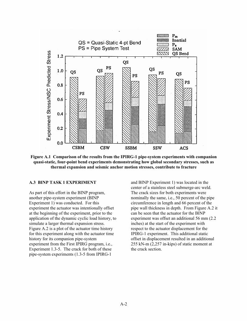
A-2

Figure A.1 Comparison of the results from the IPIRG-1 pipe-system experiments with companion

quasi-static, four-point bend experiments demonstrating how global secondary stresses, such as thermal expansion and seismic anchor motion stresses, contribute to fracture

A.3 BINP TASK 1 EXPERIMENT As part of this effort in the BINP program, another pipe-system experiment (BINP Experiment 1) was conducted. For this experiment the actuator was intentionally offset at the beginning of the experiment, prior to the application of the dynamic cyclic load history, to simulate a larger thermal expansion stress. Figure A.2 is a plot of the actuator time history for this experiment along with the actuator time history for its companion pipe-system experiment from the First IPIRG program, i.e., Experiment 1.3-5. The crack for both of these pipe-system experiments (1.3-5 from IPIRG-1

and BINP Experiment 1) was located in the center of a stainless steel submerge-arc weld. The crack sizes for both experiments were nominally the same, i.e., 50 percent of the pipe circumference in length and 66 percent of the pipe wall thickness in depth. From Figure A.2 it can be seen that the actuator for the BINP experiment was offset an additional 56 mm (2.2 inches) at the start of the experiment with respect to the actuator displacement for the IPIRG-1 experiment. This additional static offset in displacement resulted in an additional 255 kN-m (2,257 in-kips) of static moment at the crack section.

A-3

-20

0

20

40

60

80

100

0 1 2 3 4 5 6

Time, seconds

Act

uato

r Dis

plac

emen

t, m

m

BINP Task 1 Experiment High Thermal Expansion Stresses

IPIRG-1 Experiment 1.3-5Nominal Thermal Expansion Stresses

Surface Crack Penetration BINP Task 1: 0.895 seconds

Figure A.2 Actuator time history for BINP Task 1 experiment and IPIRG-1 Experiment 1.3-5

Figure A.3 is a plot of the crack section moment as a function of time for these two pipe-system experiments up to the instant when the surface crack penetrated the pipe wall thickness. From this figure it can be seen that the total moment at the crack section at the instant of surface crack penetration was comparable for the two experiments. This further supports the contention that these global secondary stresses (thermal expansion and SAM stresses) contribute just as much to fracture as do the primary stresses, at least for the case where the

stresses in the uncracked pipe are below the yield strength of the pipe. From Figure A.4, which is a similar plot as Figure A.1, except it shows the results for the four stainless steel weld experiments (Experiment 4141-4 from the Degraded Piping Program, Experiment 1.3-5 from IPIRG-1, Experiment 1-5 from IPIRG-2, and the BINP Task 1 experiment), it can be seen that the primary stresses for the BINP Task 1 experiment represented only 35 percent of the total stress at maximum load.

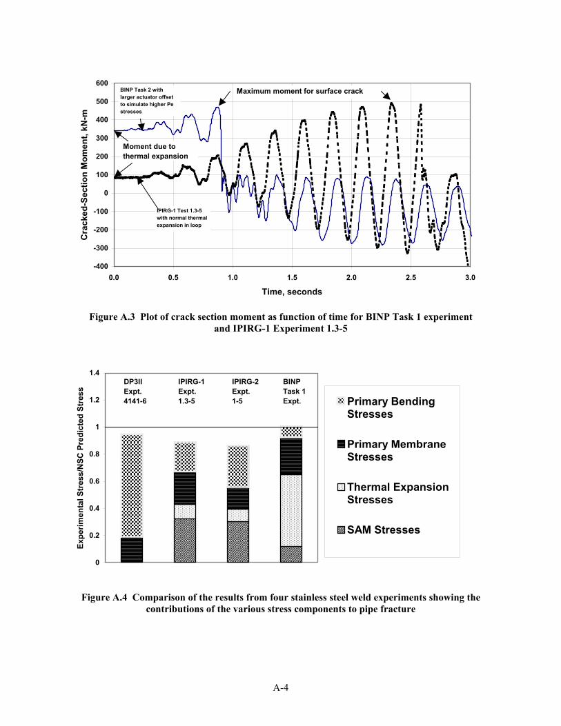
A-4

-400

-300

-200

-100

0

100

200

300

400

500

600

0.0 0.5 1.0 1.5 2.0 2.5 3.0

Time, seconds

Cra

cked

-Sec

tion

Mom

ent,

kN-m

Maximum moment for surface crack

Moment due to thermal expansion

BINP Task 2 with larger actuator offset to simulate higher Pe stresses

IPIRG-1 Test 1.3-5 with normal thermal expansion in loop

Figure A.3 Plot of crack section moment as function of time for BINP Task 1 experiment

and IPIRG-1 Experiment 1.3-5

0

0.2

0.4

0.6

0.8

1

1.2

1.4

Expe

rimen

tal S

tres

s/N

SC P

redi

cted

Str

ess

Primary BendingStresses

Primary MembraneStresses

Thermal ExpansionStresses

SAM Stresses

DP3IIExpt. 4141-6

IPIRG-1Expt. 1.3-5

IPIRG-2Expt.1-5

BINPTask 1Expt.

Figure A.4 Comparison of the results from four stainless steel weld experiments showing the

contributions of the various stress components to pipe fracture

A-5

These findings support the contention that the thermal expansion and seismic anchor motion (SAM) stresses (secondary stresses) are as detrimental as the primary stresses, at least for these test conditions for which the stresses at failure for the uncracked pipe were less than the yield strength of the material. For such conditions, there is the potential for elastic follow-up. Section III of the ASME code recognizes this potential in its local overstrain criteria in paragraph NC-3672.6(b). This paragraph implies that global secondary stresses, such as thermal expansion and seismic anchor motion stresses, can act as primary stresses under certain conditions, such as when the weaker or higher stressed portions of the piping system are subjected to strain concentrations due to elastic follow-up of the stiffer or lower stressed portions. One such obvious example of this is the IPIRG pipe system in which a large crack is introduced into a weaker material (lower yield strength) than the surrounding materials. Consequently, the resultant stresses for the uncracked pipe sections were less than the yield strength at the time of failure of the cracked section. The implication is that the safety margins for secondary stresses may be a function of the ratio of the failure stress to the yield strength. If the failure/yield stress ratio is less than 1.0, then global secondary stresses should probably be treated the same as primary stresses for fracture in the stability/critical crack size analyses. If the opposite holds true, then the global secondary stresses may become less important with some nonlinear function. A.4 REFERENCES A.1 Scott, P., Olson, R., and Wilkowski, G. Marschall, C., and Schmidt, R., “Crack Stability in a Representative Piping System Under Combined Inertial and Seismic/Dynamic Displacement-Controlled Stresses – Subtask 1.3 Final Report,” NUREG/CR-6233, Vol. 3, June 1997. A.2 Scott, P., Olson, R., Marschall, C., Rudland, D., Francini, R., Wolterman, R., Hopper, A., and Wilkowski, G., “IPIRG-2 Task 1 – Pipe System Experiments with

Circumferential Cracks in Straight-Pipe Locations,” NUREG/CR-6389, February 1997. A.3 Wilkowski, G., and others, “Degraded Piping Program – Phase II, Summary of Technical Results and Their Significance to Leak-Before-Break and In-Service Flaw Acceptance Criteria – March 1993 – December 1994,” NUREG/CR-4599, Vol. 8, March 1989. A.4 Kanninen, M., and others, “Instability Predictions for Circumferentially Cracked Type 304 Stainless Steel Pipes Under Dynamic Loadings,” EPRI Report NP-2347, April 1982.