the bear’s lair: index credit default swaps and the...
TRANSCRIPT

The Bear’s Lair: Index Credit Default Swaps and theSubprime Mortgage Crisis∗
Richard Stanton†and Nancy Wallace‡
June 1, 2011
Abstract
During the recent financial crisis, ABX.HE index credit default swaps (CDS) onbaskets of mortgage-backed securities were a benchmark widely used by financial in-stitutions to mark their subprime mortgage portfolios to market. However, we findthat prices for the AAA ABX.HE index CDS during the crisis were inconsistent withany reasonable assumption for mortgage default rates, and that these price changesare only weakly correlated with observed changes in the default performance of theunderlying loans in the index, casting serious doubt on the suitability of these CDS asvaluation benchmarks. We also find that the AAA ABX.HE index CDS price changesare related to short-sale activity for publicly traded investment banks with significantmortgage market exposure. This suggests that capital constraints, limiting the supplyof mortgage-bond insurance, may be playing a role here similar to that identified byFroot (2001) in the market for catastrophe insurance.
∗Financial support from the Fisher Center for Real Estate and Urban Economics is gratefully acknowl-edged. For helpful comments and suggestions, we thank Pierre Collin-Dufresne, Dwight Jaffee, RobertMcDonald, Atif Mian, Christine Parlour, Vikrant Vig, Matthew Spiegel (the Editor), three anonymous ref-erees, and seminar participants at BI Norwegian School of Management, the Federal Reserve Bank of NewYork, the 2009 Summer Real Estate Symposium, the 2009 RFS-Yale Conference on the Financial Crisis,the 2009 AREUEA Meeting, the 2009 AREUEA International conference, and the November 2009 NBERSecuritization Meeting.†Haas School of Business, U.C. Berkeley, [email protected].‡Haas School of Business, U.C. Berkeley, [email protected].

1 Introduction
In January 2006, a consortium of investment banks, in partnership with Markit Group
Ltd. (a data vendor), launched the Markit ABX.HE index credit default swaps (CDS).1
Each index tracks the price of a single credit default swap written on a specified basket of
subprime residential mortgage-backed securities of six different credit qualities: AAA, AA,
A, BBB, BBB-, and Penultimate AAA (PENAAA).2
While the cash flows of each ABX.HE index CDS are in principle equivalent to those
from a portfolio of CDS on each of the 20 individual named tranches of a given credit rating,
they allow market participants to trade the credit risk of a portfolio of pools via a single
security rather than via 20 separate CDS (which may not even all exist), and without having
to own, or to have borrowed, the referenced obligations. Moreover, unlike individual CDS,
the ABX.HE index CDS are supported by a consortium of market makers, ensuring that
their liquidity is substantially higher than that of either individual named CDS or (in the
over-the-counter cash markets) the referenced obligations themselves. As a result, ABX.HE
index CDS have been widely used by banks and investment banks to hedge their subprime
residential mortgage pipeline risk, and by investment banks, hedge funds and other investors
to make directional bets on the future performance of subprime mortgage-backed securities.
In particular, trading in the ABX.HE index CDS delivered two of the largest pay-outs in
the history of financial markets: the Paulson & Co. series of funds secured $12 billion in
profits from a single trade in 2007; and Goldman Sachs generated nearly $6 billion of profits
(erasing $1.5 to $2.0 billion of losses on their $10 billion subprime holdings) in 2007.3
Perhaps most important, with the global collapse of subprime mortgage-backed security
trading during the recent financial crisis, many portfolio investors in these securities began
using the more liquid ABX.HE index CDS prices as a benchmark for marking-to-market
their trading portfolios of subprime securities.4 For example, the Swiss bank UBS AG wrote
down its subprime mortgage investments by $10 billion largely based on the ABX.HE index
CDS (see UBS AG 6K financial statements). Both Morgan Stanley and Citigroup cited
1The sixteen investment banks in the consortium, CDS IndexCo LLC, are: Bank of America, BNPParibas, Deutsche Bank, Lehman Brothers, Morgan Stanley, Barclays Capital, Citigroup, Goldman Sachs,RBS, Greenwich Capital, UBS, Bear Stearns, Credit Suisse, JP Morgan, Merrill Lynch, and Wachovia.
2PENAAA is a relatively new ABX.HE index CDS, written on the penultimate AAA bond in the mortgagestructure. This bond has a shorter duration (and hence less interest-rate risk) than the longer-duration AAAbonds tracked by the AAA ABX.HE index CDS.
3For details, see Kelly (December 14, 2007), Mackintosh (January 15, 2008), Zuckerman (January 15,2008), and Lewis (February 16, 2008).
4Articles discussing the use of these CDS as benchmarks for pricing include Economist (March 8, 2008),Ng, Mollenkamp, and Patterson (2007), Bank of England (2008), Senior Supervisors Group (2008), Wood(2008), Logan (2008), “More than just a technical hitch,” Credit, Sept. 2007, “One-way fear,” Risk Magazine,Feb. 1, 2008, “Putting a price on subprime assets,” Stewart Eisenhart, Risk Magazine, Oct. 1, 2007.
1
devaluations in the ABX.HE index CDS to justify their significant write-downs of subprime
securities (see Ng et al., 2007). Most recently, in August 2010 Goldman submitted a nine-
page memo to the Financial Crisis Inquiry Commission (see Goldman Sachs, 2010) describing
how it used ABX.HE prices in 2007 and 2008 in setting the CDO prices it quoted when
demanding over $12 billion in collateral payments from the insurance firm AIG.5 Finally, in
March 2008, the Division of Corporation Finance of the Securities and Exchange Commission
sent public companies an illustrative letter with preparation guidelines for the Management’s
Discussion and Analysis (MD&A) statements required for Form 10-K quarterly reports. The
letter suggested that:
“Regardless of how you have classified your assets and liabilities within the
SFAS 157 hierarchy, if you have not already done so in your Form 10-K, consider
providing the following additional information in your MD&A:
• A general description of the valuation techniques or models you used with
regard to your material assets or liabilities. Consider describing any material
changes you made during the reporting period to those techniques or models,
why you made them, and, to the extent possible, the quantitative effect of
those changes.
• To the extent material, a discussion of the extent to which, and how, you
used or considered relevant market indices, for example ABX or CMBX, in
applying the techniques or models you used to value your material assets or
liabilities. Consider describing any material adjustments you made during
the reporting period to the fair value of your assets or liabilities based on
market indices and your reasons for making those adjustments . . . ”6
During the crisis, there were many who claimed that ABX prices were out of line with
fundamentals or otherwise unrepresentative of prices for the entire MBS market (see, for
5On page 3, Goldman describes how “. . . it was not unusual for there to be an absence of transactions inspecific RMBS [residential mortgage-backed securities], CDO [collateralized debt obligations] securities andderivatives. In addition, certain securities often had only one or a limited numbers of holders. As a result, weused observed transactions in comparable instruments (e.g., instruments having similar underlying collateral,structure, and/or risk/reward profile) to help inform our valuations.” It then describes (page 4) how “Alsoshown are two indices referencing subprime securities issued in the second half of 2005 – the double-A ratedand triple-B rated tranches of the ABX 06-1 index. These indices represented the most liquid and observableproxy for the vintage and ratings of the RMBS underlying the AIG CDO positions.” Ng and Mollenkamp(2010) discuss Goldman’s use of the ABX.HE index CDS, saying “Goldman also cited prices of the ABX, anindex that was made up of derivatives tied to a basket of 20 subprime mortgage bonds issued in 2005, theyear many of the AIG-insured CDOs were created. The index was generally regarded by market participantsas a rough proxy for the values of subprime mortgage bonds that were the underlying assets of CDOs.”
6See Sample Letter Sent to Public Companies on MD&A Disclosure Regarding the Application of SFAS157 (Fair Value Measurements), http://www.sec.gov/divisions/corpfin/guidance/fairvalueltr0308.htm.
2

example, Bank of England, 2008; Economist, March 8, 2008; Fender and Hoerdahl, 2008).
To investigate this in more detail, we collect detailed credit and prepayment histories from
2006–2010 for all of the roughly 360,000 individual loans underlying the ABX.HE index
CDS, and use these data, plus prices from June 2009, to infer the market’s expectations for
future defaults at the height of the recent crisis. Using both a simple, “back-of-the-envelope”
model (in which all defaults and insurance payments occur instantaneously) and a full CDS
valuation model calibrated to historical loan-level performance data, we find that recent price
levels for AAA ABX.HE index CDS are inconsistent with any reasonable forecast for the
future default performance of the underlying loans. For example, assuming a prepayment
rate of 25% per year (roughly consistent with historical prepayment rates on these pools),
at a recovery rate of 34%, the AAA ABX.HE prices on June 30, 2009 imply default rates
of 100% on the underlying loans. In other words, if recovery rates exceed 34% (a value
well below anything ever observed in U.S. mortgage markets), there is no default rate high
enough to support observed prices. We also find that changes in the credit performance of
the underlying loans explain almost none of the observed price changes in the AAA ABX.HE
index CDS, in contrast to previous research, such as Fender and Scheicher (2008). These
results cast serious doubt on the use of the AAA ABX.HE index CDS for marking mortgage
portfolios to market.
While ABX.HE price changes are unrelated to credit performance, we find that they
are consistently and significantly related to short-sale activity in the equity markets of the
publicly traded investment banks. These measures may be proxying for the demand for
default insurance on mortgage-backed securities, suggesting that, as in the catastrophe in-
surance market (see Froot, 2001), shifts in the demand for default insurance provided by the
ABX.HE index CDS, combined with limited capital behind the providers of this insurance,
may be driving the price of such insurance well above its “fair value.”
2 ABX.HE index CDS prices and implied default rates
Each ABX.HE index CDS tracks the price of a single credit default swap (CDS) written on a
fixed basket of underlying mortgage-backed securities. The first set, or vintage, of ABX.HE
index CDS began trading in January of 2006, and a new vintage began trading every six
months from then until July 2007.7 The four currently outstanding vintages are labeled
ABX.HE-2006-1, ABX.HE-2006-2, ABX.HE-2007-1, and ABX.HE-2007-2 respectively.
7The ABX.HE index CDS were originally designed to be issued every six months. However, due to thesevere disruptions in the market for subprime mortgage-backed securities, the ABX.HE-2008-1 series (dueto be issued in January 2008) was canceled, and no subsequent ABX.HE index CDS have been issued.
3
The construction of each vintage of ABX.HE index CDS starts with the selection of 20
specified pools of subprime residential mortgage-backed securities by Markit. The subprime
residential mortgages included in the ABX.HE index CDS are required to meet fixed criteria
concerning pool composition and loan quality. Markit Group Ltd. and the consortium of
member-dealers constrain the basket to include only four deals from the same originator, and
no more than six deals can have the same servicer. The minimum deal size must be $500
million, the pools must consist of at least 90% first liens, and the average FICO score8 of
the borrowers must be at least 660. The referenced AAA tranche is the longest bond in the
sequence of AAA bonds in a typical pool structure, and it must have an average life greater
than five years. The average life for the referenced subordinated tranches must be four
years. Although each of the ABX.HE index CDS is made up of the same twenty referenced
obligations, over time the notional balances of the underlying CDS amortize following the
principal pay-down structure of the respective referenced classes.9
The buyer of an ABX.HE CDS pays a one-time up-front fee plus a monthly premium, in
exchange for payments in the event of defaults. The quoted “price” is defined as par minus
the up-front fee. Thus, for example, a quoted price of $100 means the up-front fee is $0 (as
is the case on the issue date), and a quoted price of $70 means the up-front fee is $30.10
When the ABX.HE index CDS trades below par, the market cost of default risk protection
on subprime mortgages has increased since the issuance date of the index. For example, if
the price of the ABX.HE index CDS was quoted as 80% of par, the protection buyer would
pay the protection seller an up-front fee of 20% of the notional amount to be insured in
addition to the monthly fixed premium on the index.
For the CDS contract to be fairly priced at date t, the present value of the fixed leg plus
the single up-front payment paid by the protection buyer must equal the present value of
the floating leg paid by the protection seller, i.e.,
Bt (Par − PABX)
100+ EQ
[s
n∑k=kt
BTk−1e−
∫ Tkt rτ dτ
]=
EQ
n∑k=kt
(BTk−1
[BATk
BATk−1
− PrepayTk
]−BTk
)(1−R + i)e−
∫ Tkt rτ dτ , (1)
8FICO is an acronym for the Fair Isaac Corporation, the creators of the FICO score. The FICO scoreis a credit score based on a borrower’s payment history, current level of indebtedness, types of credit used,length of credit history, and amount of recently issued credit. FICO scores range between 300 and 850.
9For additional details on the construction of the ABX.HE index CDS, see Kazarian, Mingelgrin, Risa,Huang, Ciampini, and Brav (2005).
10If the market price of the ABX.HE contract is at a premium, the protection seller makes a one-timepayment to the protection buyer
4
where all expectations are under the “risk-neutral” probability measure. The first term
of the left-hand side of equation (1) is the protection buyer’s up-front fee payment. It is
the difference between par and the quoted market price of the ABX.HE index CDS, PABX ,
times the current notional amount of the insurance, Bt. The second term is the value of
the protection buyer’s fixed payment leg. This comprises a coupon, paid at the end of each
month Tk (starting at date Tkt , the end of the month containing date t) equal to a fixed
coupon rate, s, times the start-of-month notional, BTk−1, of the referenced bonds. The right-
hand side of equation (1) is the value of the floating leg of the ABX.HE index CDS, paid
by the protection seller to the protection buyer. It includes a payment at each date Tk to
compensate for any lost principal during the prior month. Here, BTk denotes the notional
value at date Tk, BATk
denotes the scheduled notional (taking amortization into account),
and PrepayTk is the fraction of the start-of-month principal prepaid during the month. The
difference between BTk and BTk−1, adjusted for amortization and prepayment, reflects loss
of principal due to default, which is governed by the likelihood of default on the underlying
mortgages and the structure of the pool underlying the ABS. The ABS pays off the lost
principal, net of recovery, R, plus the interest shortfall, i. On the issue date of the new
ABX.HE index CDS (t = 0), the fixed coupon rate is set so the market price of the ABX.HE
equals par, i.e., PABX = 0. As expectations of default rates vary over time, the market price,
PABXt , varies to keep the values of the two sides of the swap equal.
Figure 1 shows quoted market prices from January 19, 2006 to July 30, 2010 for the four
vintages of the AAA ABX.HE index CDS.11 It can be seen that there was little variation
in these prices until July 2007, when the poor performance of two Bear Stearns’ subprime
CDOs became public. After July 2007, the prices continued to trend downward through
June 2009. We are focusing on the AAA bonds because the primary mark-to-market losses
in the balance sheets of the commercial banks, investment banks, and structured investment
vehicles (SIVs) were related to AAA residential mortgage-backed securities.
The quoted price as of June 30, 2009 for the ABX.HE 2006-2 index was $33.165. This
price means that protection buyers were paying $66.835 per $100 of principal for the privilege
of making additional periodic payments to insure themselves against default losses on the
AAA tranche. To see that something needs explaining here, consider that, as of July, 2009,
the cumulative loss rate on the pools underlying all of the 2006-2 ABX.HE index CDS was
under 10% and was 0% for the AAA bonds. Of course, even though the recent financial
(and real estate) crisis was the worst the U.S. had seen in decades, these are only realized
11In calculating these prices, Markit collects CDS prices from the market makers, who have some discretionin reporting trades. They drop the highest and lowest of the reported prices, and average the rest. Similarpatterns (not shown) exist for the lower-rated securities.
5

Figure 1: Prices for the bonds with AAA credit ratings for the 2006 and 2007 MarkitABX.HE index CDS.
This Figure plots the Markit ABX.HE index CDS for the AAA ABX.HE-2006-1, AAA ABX.HE-
2006-2, AAA ABX.HE-2007-1, and AAA ABX.HE–2007–1 Series from January 19, 2006 to July
30, 2010.
0.000
20.000
40.000
60.000
80.000
100.000
120.000
19-Jan-06 19-Jan-07 19-Jan-08 19-Jan-09 19-Jan-10
AAA_2006_1 AAA_2006_2 AAA_2007_1 AAA_2007_2
6

default rates, and it is possible that market expectations were for much worse to come. We
therefore now infer from these prices what they imply for expected future default rates, and
compare these with what we observed during the worst financial crisis this century, the Great
Depression.
2.1 A “back-of-the-envelope” valuation model
Given a valuation model and assumptions about default rates, we can calculate the fair
up-front payment for the ABX.HE index CDS. Conversely, given a valuation model and a
market price, we can infer something about the market’s expectations about default rates.
Before developing a formal model, we start with a simple “back-of-the-envelope” model,
which strongly suggests that expected future defaults are not going to be able to explain the
prices shown in Figure 1.
Expressing all quantities per $1 of current principal, let the subordination level on the
AAA security be S,12 and assume that a proportion H of the loans are of higher seniority
than the AAA tranche,13 so the AAA balance starts at
1−H − S.
Now assume that a (known) fraction Y < H of the underlying mortgages prepays immedi-
ately, lowering the total pool balance per initial dollar to 1 − Y , and a fraction D of the
remaining mortgages then defaults. We assume no further default or prepayment, and also
ignore the periodic fixed payment made by the protection buyer. In this case, if the recovery
rate on defaulted loans is R, the defaults reduce the total principal by D(1 − R)(1 − Y ),
hence reducing the AAA principal by a fraction14
min
(1,max
{D(1−R)(1− Y )− S
1−H − S, 0
}). (2)
The fair lump-sum price (per $1 of principal) for default insurance on the AAA tranches
equals the loss, and the NPV of the security is thus
NPV = min
(1,max
{D(1−R)(1− Y )− S
1−H − S, 0
})− (1− P ). (3)
12In other words, a fraction S of the total principal on the loans must be completely lost before anyadditional losses affect the AAA tranches.
13The AAA tranche underlying the ABX.HE index CDS is the lowest-seniority AAA tranche.14The max and min in this expression account for the possibility that either all or none of the AAA
principal might be lost.
7
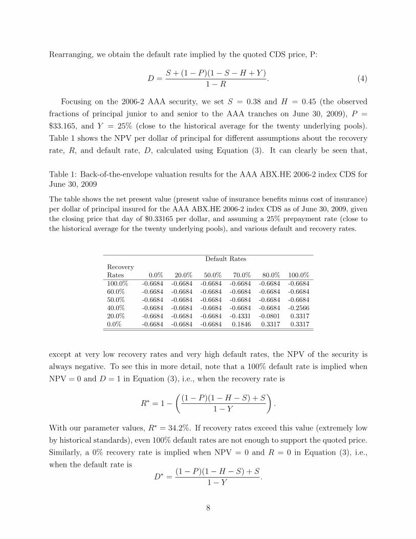
Rearranging, we obtain the default rate implied by the quoted CDS price, P:
D =S + (1− P )(1− S −H + Y )
1−R. (4)
Focusing on the 2006-2 AAA security, we set S = 0.38 and H = 0.45 (the observed
fractions of principal junior to and senior to the AAA tranches on June 30, 2009), P =
$33.165, and Y = 25% (close to the historical average for the twenty underlying pools).
Table 1 shows the NPV per dollar of principal for different assumptions about the recovery
rate, R, and default rate, D, calculated using Equation (3). It can clearly be seen that,
Table 1: Back-of-the-envelope valuation results for the AAA ABX.HE 2006-2 index CDS forJune 30, 2009
The table shows the net present value (present value of insurance benefits minus cost of insurance)
per dollar of principal insured for the AAA ABX.HE 2006-2 index CDS as of June 30, 2009, given
the closing price that day of $0.33165 per dollar, and assuming a 25% prepayment rate (close to
the historical average for the twenty underlying pools), and various default and recovery rates.
Default RatesRecoveryRates 0.0% 20.0% 50.0% 70.0% 80.0% 100.0%100.0% -0.6684 -0.6684 -0.6684 -0.6684 -0.6684 -0.668460.0% -0.6684 -0.6684 -0.6684 -0.6684 -0.6684 -0.668450.0% -0.6684 -0.6684 -0.6684 -0.6684 -0.6684 -0.668440.0% -0.6684 -0.6684 -0.6684 -0.6684 -0.6684 -0.256620.0% -0.6684 -0.6684 -0.6684 -0.4331 -0.0801 0.33170.0% -0.6684 -0.6684 -0.6684 0.1846 0.3317 0.3317
except at very low recovery rates and very high default rates, the NPV of the security is
always negative. To see this in more detail, note that a 100% default rate is implied when
NPV = 0 and D = 1 in Equation (3), i.e., when the recovery rate is
R∗ = 1−(
(1− P )(1−H − S) + S
1− Y
).
With our parameter values, R∗ = 34.2%. If recovery rates exceed this value (extremely low
by historical standards), even 100% default rates are not enough to support the quoted price.
Similarly, a 0% recovery rate is implied when NPV = 0 and R = 0 in Equation (3), i.e.,
when the default rate is
D∗ =(1− P )(1−H − S) + S
1− Y.
8

With our parameter values, D∗ = 65.8%. If the default rate is lower than this value, even a
0% recovery rate is not enough to support the quoted price.15
Comparison with historical housing crises To emphasize how extreme these numbers
are, we here look at historical U.S. mortgage loss rates to look for the “worst imaginable”
performance, and find that default and recovery rates in the US have never been bad enough
to rationalize the ABX prices we observe.
An obvious benchmark for the “worst imaginable” mortgage performance is the Great
Depression, which was used as the basis for the worst-case assumptions underlying Standard
and Poor’s original mortgage loan-loss model from the mid-1970s, as well as Moody’s original
loan-loss model from the 1980s (see Standard and Poor’s, 1993; Lowell, 2008).16 Standard
and Poor’s (1993) report that S&P based their analysis on Saulnier (1950), who analyzes
the performance of mortgages issued by 24 leading life insurance companies between 1920
and 1946. The highest lifetime foreclosure rates (see Table 22), on loans issued in 1928 and
1929, reached 28.5% and 29.6% respectively.17 Losses on foreclosed properties varied by
date of disposal, but for loans issued between 1925 and 1929 did not exceed 12% (Table 27).
Combined, these foreclosure and loss rates are not sufficient to generate any losses in the
AAA ABX tranches, given the subordination levels we see in our sample.
Another, more recent, “worst-case” benchmark is the performance of loans in the “Oil
Patch” states in the 1980s, which was actually worse than overall loan performance during
the Great Depression. By law, in evaluating the capital adequacy of Freddie Mac and Fannie
Mae, OFHEO (now FHFA) was required to assume a benchmark loss experience equal to
the worst cumulative losses experienced during any two-year period in contiguous states
containing in total at least 5% of the U.S. population.18 The latest benchmark was based
on loans originated in Arkansas, Louisiana, Mississippi and Texas during 1983 and 1984
(representing 5.3% of the U.S. population), just before the oil price collapse of 1986. Average
cumulative default rates for these loans were 14.9%, with an average 10-year loss severity
across the region of 63.3%, leading to average cumulative 10-year losses of 9.4%.19 Sorted by
15While extreme, our results here are actually somewhat understated. We have assumed that the seniortranches prepay earlier and default later than the ABX.HE AAA tranche. In fact, in several of the deals,while prepayment does indeed hit the more senior tranches first, default is equally shared among all of theAAA tranches, including the more senior tranches. Thus our calculations overestimate the default rate onthe ABX.HE AAA tranche. We take all of these detailed tranche-by-tranche allocation rules into account inimplementing our Monte Carlo valuation model below.
16Excellent discussions of mortgage performance during the Great Depression can be found in Bridewell(1938), Harriss (1951), Wheelock (2008a,b) and Rose (2010).
17These figures are at least as high as those (from a different source) reported in Snowden (2006).18For details, see Davidson, Sanders, Wolff, and Ching (2003, pp. 310–313), Lowell (2008) or Kinsey (1998).19“Default” as used here by OFHEO means that a loan completed foreclosure or otherwise resulted in a
realized loss of principal. It does not include loans that were merely delinquent.
9

LTV, the losses are highest for high-LTV loans, with > 90% LTV loans experiencing 26.4%
default rates and 69.0% loss rates, for a cumulative 10-year loss of 18.2%. Even if the whole
country saw the same loss levels as these > 90% LTV Oil Patch loans from 1983–1984, it
would not be enough to trigger losses in the AAA ABX.HE index CDS.
There are, of course, differences between the loans considered above and those underlying
the ABX. In particular, these were not subprime loans. However, while default rates are
probably higher on subprime than on prime loans, there are several other offsetting biases:
i. The failure of thousands of banks and other financial institutions during the Depression
meant that even many good borrowers could not refinance and therefore entered financial
distress. ii. the 1983–1984 loans in Arkansas, Louisiana, Mississippi and Texas were the worst
performing loans in the country, so country-wide default and loss rates were substantially
lower. In our analysis, we conservatively consider the effect of country-wide losses at these
same levels. iii. By focusing on the 1983–1984 default statistics for loans with LTV > 90%,
we are automatically looking at loans with default rates higher than average, which should
correct for a large part of the difference between prime and subprime loans. iv. Although
delinquency rates were extremely high during the Great Depression, eventual loss rates on
these loans were relatively low, certainly compared with the Oil Patch loans during the 1980s
discussed above.20 One important reason for this is that Federal and state governments took
steps to limit losses to lenders, such as the creation of the Home Owners’ Loan Corporation
(HOLC) in 1933 (see Rose, 2010). This agency bought huge numbers of loans from lenders
at inflated prices (many lenders escaped loss entirely), then the HOLC issued new loans to
the borrowers with 15 years to maturity and a 5% (later 4.5%) interest rate. Any estimate
of future expected losses during the recent crisis has to take into account the likelihood that
Federal or state governments would take similar actions to mitigate lenders’ losses should
mortgage performance become bad enough.
2.2 Realized prepayments and losses
Tables 2 and 3 summarize the realized prepayment and default performance for the eighty
pools tracked by the four ABX.HE index CDS. Looking first at the performance of the pools
as a whole, it is clear from Table 2 that the most important cause of principal pay-down for
the 2006 vintage pools through July 30, 2010, was early return of principal, i.e., prepayment.
The average cumulative amount of prepaid principal was 59.11% for the 2006-1 pools, and
54% for the 2006-2 pools. Table 3 shows that the average cumulative prepayment speed for
the 2007-1 and 2007-2 ABX.HE pools was 34.55% and 23.12%, respectively.
20According to Bridewell (1938) and Wheelock (2008b), at the beginning of 1934, roughly half of all homeswith an outstanding mortgage were delinquent, with an average time of delinquency of 15–18 months.
10

The amount of principal lost was a fraction of these amounts. For the 2006-1 pools, the
average cumulative loss percentage was 13.79%, ranging from 5.48% to about 25%. The
average cumulative loss percentage for the 2006-2 pools was higher at 14.36%, ranging from
5.67% to 28.21%. Losses for the 2007 vintage were somewhat higher. The average for the
2007-1 pools was 17.62%, ranging from 4.40% to 26.07%, and was 19.61% for the 2007-2
pools, ranging from 13.39% to 33.94%. Recovery rates average between 35% and 40% for
the different vintages.21
Looking now at the performance of the AAA tranches (shown in the last two columns
of the tables), we see that for the AAA ABX.HE 2006-1, the average cumulative percentage
of principal prepaid through July 30, 2010 was about 20.67%, and was 1.88% for the AAA
ABX.HE 2006-2. The prepayment speeds for the AAA tranches for the 2007 vintage pools
were effectively 0%, with only one pool, ACE 2007-HE4, experiencing a 5% cumulative
principal payoff rate. There were no principal losses on any of these AAA tranches.22
21Not all recovery rates are available as, in some cases, Lewtan ABSNet report the recovery rate as NA.22Although not shown in the table, Lewtan ABSNet data continue to show no principal losses for any
AAA tranche in any vintage through December 27, 2010.
11

Tab
le2:
Dea
lst
ruct
ure
,lo
ssan
dpre
pay
men
tp
erfo
rman
ceof
the
pool
sin
the
Mar
kit
AB
X.H
E20
06-1
and
2006
-2In
dex
CD
S
Th
eta
ble
sum
mar
izes
the
dea
lst
ruct
ure
for
the
twen
typ
ools
that
make
up
the
AB
X.H
E2006-1
(up
per
pan
el)
an
dA
BX
.HE
2006-2
(low
erp
an
el)
ind
exC
DS
.T
he
tab
lep
rese
nts
the
nam
eof
the
Dep
osi
tor,
the
dea
ln
am
e,th
eto
tal
nu
mb
erof
tran
ches
inea
chp
ool,
the
tota
lp
ool
pri
nci
pal
at
issu
ance
,an
dth
eou
tsta
nd
ing
pool
pri
nci
pal
onJu
ly30,
2010.
Th
eta
ble
als
ore
port
sth
ecu
mu
lati
vep
rep
aid
pri
nci
pal
(mea
sure
das
the
per
centa
ge
ofin
itia
lto
tal
pool
pri
nci
pal
),cu
mu
lati
velo
sses
(mea
sure
das
the
per
centa
ge
of
init
ial
tota
lp
ool
pri
nci
pal)
,an
dcu
mu
lati
vere
cove
ryra
tes
(mea
sure
d
asa
per
centa
geof
gros
slo
sses
)fo
rea
chp
ool
asof
Ju
ly30,
2010.
Th
ela
sttw
oco
lum
ns
of
the
table
pre
sent
the
cum
ula
tive
pre
paid
pri
nci
pal
an
dth
e
cum
ula
tive
loss
esfo
rth
eA
AA
tran
che
ofea
chp
ool.
Th
ere
port
edd
ata
wer
eob
tain
edfr
om
Lew
tan
AB
SN
et.
AAA
AAA
Tota
lPool
Tota
lPool
Tota
lPool
ABX.H
EABX.H
EPrincip
al
Cumulative
Cumulative
Cumulative
Cumulative
Cumulative
Number
at
Princip
al
Pre
paid
NetLoss
Recovery
Pre
paid
Loss
Deposito
rDeal
of
Issu
ance
7/2010
7/2010
7/2010
7/2010
7/2010
7/2010
Name
Name
Tra
nches
($M
)($
M)
(%)
(%)
(%)
(%)
(%)
ABX.H
E2006-1
AceSecuritiesCorp
ora
tion
ACE
2005-H
E7
21
1737
377.45
59.93
18.61
39.58
0.00
0.00
Ameriquest
MortgageSecurities
AM
SI2005-R
11
19
1454
598.87
51.72
7.23
35.21
0.00
0.00
Arg
entAssetPass-T
hro
ugh
Cert.
ARSI2005-W
222
2697
713.58
61.06
12.61
32.24
0.00
0.00
BearSte
arn
sAssetBacked
Sec.Tru
stBSABS
2005-H
E11
30
603
191.37
57.13
11.37
36.41
0.00
0.00
Countrywid
eAssetBacked
Tru
stCW
L2005-B
C5
18
922
301
58.85
6.35
59.61
0.00
0.00
CS
First
Boston
HomeEquity
AssetTru
stHEAT
2005-8
23
1462
322.71
53.18
14.62
41.16
0.00
0.00
First
Fra
nklin
MortgageLoans
FFM
L2005-F
F12
16
1027
563.11
30.55
14.62
46.62
0.00
0.00
Gold
man
SachsGSAM
PTru
stGSAM
P2005-H
E4
20
1413
311.03
56.34
11.45
40.62
63.29
0.00
J.P
.M
org
an
Mort.Acquisition
Tru
stJPM
AC
2005-O
PT1
30
1447
276.5
70.65
5.98
43.60
79.32
0.00
Long
Beach
MortgageLoan
Tru
stLBM
LT
2005-W
L2
26
2651
494.28
70.84
11.46
40.08
72.34
0.00
MasterAssetBacked
Sec.Tru
stM
ABS
2005-N
C2
20
887
205.6
57.98
18.84
41.58
0.00
0.00
MerrillLynch
MortgageIn
vest.Tru
stM
LM
I2005-A
R1
17
1062
224.37
60.75
9.53
43.71
49.71
0.00
Morg
an
Sta
nley
CapitalIn
c.
MSAC
2005-H
E5
16
1428
281.33
69.23
11.26
32.19
66.45
0.00
New
Centu
ryHomeEquity
Tru
stNCHET
2005-4
14
2005
566.85
63.71
10.98
46.10
0.00
0.00
ResidentialAssetM
ort.Pro
d.In
c.
RAM
P2005-E
FC4
16
708
170.98
64
11.88
NA
0.00
0.00
ResidentialAssetSecuritiesCorp
.RASC
2005-K
S11
19
1339
368.27
58.17
14.34
38.14
0.00
0.00
Security
AssetBacked
ReceivablesIn
c.
SABR
2005-H
E1
18
711
222.54
52.28
16.61
33.44
46.60
0.00
Soundview
HomeEquity
Loan
Tru
stSVHE
2005-4
19
834
251.82
56.7
13.25
38.05
14.80
0.00
Structu
red
AssetIn
vest.Loan
Tru
stSAIL
2005-H
E3
20
2291
436.4
61.82
10.98
44.60
18.74
0.00
Structu
red
AssetSecurity
Corp
.SASC
2005-W
F4
17
1896
514.75
67.37
5.60
36.85
2.18
0.00
Mean
20.05
1428.70
369.64
59.11
11.88
40.51
20.67
0.00
Sta
ndard
Deviation
4.37
624.84
157.26
8.80
3.80
6.37
29.57
0.00
ABX.H
E2006-2
AceSecuritiesCorp
ora
tion
ACE
2006-N
C1
16
1324
356.29
56.74
16.35
30.56
0.00
0.00
Arg
entAssetPass-T
hro
ugh
Cert.
ARSI2006-W
116
2275
591.97
54.34
19.64
34.22
0.00
0.00
BearSte
arn
sAssetBacked
Sec.Tru
stBSABS
2006-H
E3
13
793
223.11
57.35
14.52
39.65
0.00
0.00
Carrin
gto
nM
ortgageLoan
Tru
stCARR
2006-N
C1
14
1463
701.97
47.79
4.23
49.68
0.00
0.00
Countrywid
eAssetBacked
Tru
stCW
L2006-8
16
2000
969.23
41.39
10.15
39.14
0.00
0.00
CS
First
Boston
HomeEquity
AssetTru
stHEAT
2006-4
18
1585
473.47
51.54
15.54
36.97
0.00
0.00
First
Fra
nklin
MortgageLoans
FFM
L2006-F
F4
14
1534
461.54
55.62
14.29
44.13
0.00
0.00
Gold
man
SachsGSAM
PTru
stGSAM
P2006-H
E3
17
1632
491.47
58.6
11.29
NA
0.00
0.00
J.P
.M
org
an
Mort.Acquisition
Tru
stJPM
AC
2006-F
RE1
16
1013
285.38
65.9
16.12
38.28
0.00
0.00
Long
Beach
MortgageLoan
Tru
stLBM
LT
2006-1
17
2500
680.36
61.45
11.33
38.16
0.00
0.00
MasterAssetBacked
Sec.Tru
stM
ABS
2006-N
C1
16
915
264.99
55.25
15.79
37.12
0.00
0.00
MerrillLynch
MortgageIn
vest.Tru
stM
LM
I2006-H
E1
18
764
219.59
61.72
18.17
NA
0.00
0.00
Morg
an
Sta
nley
CapitalIn
c.
MSAC
2006-H
E2
16
2266
609.61
55.16
17.94
37.56
0.00
0.00
Morg
an
Sta
nley
CapitalIn
c.
MSAC
2006-W
MC2
15
2603
557.76
50.36
28.21
32.57
6.19
0.00
ResidentialAssetM
ort.Pro
d.In
c.
RAM
P2006-N
C2
14
760
240.05
51.15
17.26
34.12
0.00
0.00
ResidentialAssetSecuritiesCorp
.RASC
2006-K
S3
17
1150
331.93
53.51
17.62
34.91
0.00
0.00
Security
AssetBacked
ReceivablesIn
c.
SABR
2006-O
P1
14
1260
320.54
68.89
5.67
47.26
31.43
0.00
Soundview
HomeEquity
Loan
Tru
stSVHE
2006-O
PT5
18
3100
1172.16
45.25
14.68
34.52
0.00
0.00
Structu
red
AssetIn
vest.Loan
Tru
stSAIL
2006-4
16
1699
814.51
32.65
19.41
35.02
0.00
0.00
Structu
red
AssetSecurity
Corp
.SASC
2006-W
F2
15
1299
456.87
52.3
12.53
NA
0.00
0.00
Mean
15.80
1596.75
511.14
53.85
15.04
37.88
1.88
0.00
Sta
ndard
Deviation
1.47
669.39
259.04
8.22
5.19
5.07
7.09
0.00
12

Tab
le3:
Dea
lst
ruct
ure
,lo
ssan
dpre
pay
men
tp
erfo
rman
ceof
the
pool
sin
the
Mar
kit
AB
X.H
E20
07-1
and
2007
-2In
dex
CD
S
Th
eta
ble
sum
mar
izes
the
dea
lst
ruct
ure
for
the
twen
typ
ools
that
make
up
the
AB
X.H
E2007-1
(up
per
pan
el)
an
dA
BX
.HE
2007-2
(low
erp
an
el)
ind
exC
DS
.T
he
tab
lep
rese
nts
the
nam
eof
the
Dep
osi
tor,
the
dea
ln
am
e,th
eto
tal
nu
mb
erof
tran
ches
inea
chp
ool,
the
tota
lp
ool
pri
nci
pal
at
issu
ance
,an
dth
eou
tsta
nd
ing
pool
pri
nci
pal
onJu
ly30,
2010.
Th
eta
ble
als
ore
port
sth
ecu
mu
lati
vep
rep
aid
pri
nci
pal
(mea
sure
das
the
per
centa
ge
ofin
itia
lto
tal
pool
pri
nci
pal
),cu
mu
lati
velo
sses
(mea
sure
das
the
per
centa
ge
of
init
ial
tota
lp
ool
pri
nci
pal)
,an
dcu
mu
lati
vere
cove
ryra
tes
(mea
sure
d
asa
per
centa
geof
gros
slo
sses
)fo
rea
chp
ool
asof
Ju
ly30,
2010.
Th
ela
sttw
oco
lum
ns
of
the
table
pre
sent
the
cum
ula
tive
pre
paid
pri
nci
pal
an
dth
e
cum
ula
tive
loss
esfo
rth
eA
AA
tran
che
ofea
chp
ool.
Th
ere
port
edd
ata
wer
eob
tain
edfr
om
Lew
tan
AB
SN
et.
AAA
AAA
Tota
lPool
Tota
lPool
Tota
lPool
ABX.H
EABX.H
EPrincip
al
Cumulative
Cumulative
Cumulative
Cumulative
Cumulative
Number
at
Princip
al
Pre
paid
NetLoss
Recovery
Pre
paid
Loss
Deposito
rDeal
of
Issu
ance
7/2010
7/2010
7/2010
7/2010
7/2010
7/2010
Name
Name
Tra
nches
($M
)($
M)
(%)
(%)
(%)
(%)
(%)
ABX.H
E2007-1
ACE
SecuritiesCorp
ora
tion
ACE
2006-N
C3
20
1461
825.6
28.23
15.26
NA
0.00
0.00
AssetBacked
Fundin
gCorp
ora
tion
ABFC
2006-O
PT2
20
1061
477.6
39.76
15.22
40.85
0.00
0.00
BearSte
arn
sAssetBacked
Sec.Tru
stBSABS
2006-H
E10
14
1096
638.36
25.87
15.89
33.36
0.00
0.00
Carrin
gto
nM
ortgageLoan
Tru
stCARR
2006-N
C4
19
1551
1050.62
27.86
4.4
39.82
0.00
0.00
Citigro
up
MortgageLoan
Tru
stCM
LTI2006-W
FH3
19
1563
674.85
44.78
12.05
36.53
0.00
0.00
Countrywid
eHomeLoans
CW
L2006-1
817
1653
969.23
31.21
10.15
38.59
0.00
0.00
Cre
dit
Base
dAssetServ
icin
gand
Sec.
CBASS
2006-C
B6
20
734
307.43
41.02
17.09
35.54
0.00
0.00
CS
First
Boston
HomeEquity
AssetTru
stHEAT
2006-7
19
1070
383.56
38.08
26.07
38.42
0.00
0.00
First
Fra
nklin
MortgageLoans
FFM
L2006-F
F13
22
2055
916.69
37.68
17.71
40.85
0.00
0.00
Fre
montHomeLoan
Tru
stFHLT
2006-3
19
1574
627.23
43.32
16.83
29.61
0.00
0.00
Gold
man
SachsGSAM
PTru
stGSAM
P2006-H
E5
21
996
408.88
38.45
19.84
NA
0.00
0.00
J.P
.M
org
an
Mort.Acquisition
Tru
stJPM
AC
2006-C
H2
15
1964
1149.49
30.42
11.06
31.38
0.00
0.00
Long
Beach
MortgageLoan
Tru
stLBM
LT
2006-6
21
1645
629.22
36.2
25.55
32.32
0.00
0.00
MasterAssetBacked
Sec.Tru
stM
ABS
2006-N
C3
20
999
429.12
33.24
23.8
31.52
0.00
0.00
MerrillLynch
MortgageIn
vest.Tru
stM
LM
I2006-H
E5
15
1319
588.55
33.48
21.9
31.73
0.00
0.00
Morg
an
Sta
nley
CapitalIn
c.
MSAC
2006-H
E6
18
1429
722.3
31.1
18.35
31.86
0.00
0.00
ResidentialAssetSecuritiesCorp
.RASC
2006-K
S9
16
1197
552.76
31.84
21.98
27.52
0.00
0.00
Security
AssetBacked
ReceivablesIn
c.
SABR
2006-H
E2
17
678
352.35
24.77
23.26
NA
0.00
0.00
Soundview
HomeEquity
Loan
Tru
stSVHE
2006-E
Q1
19
1692
710.21
40.81
17.21
31.50
0.00
0.00
Structu
red
AssetSecurity
Corp
.SASC
2006-B
C4
18
1529
749.97
32.87
18.08
NA
0.00
0.00
Mean
18.45
1363.30
658.20
34.55
17.59
34.46
0.00
0.00
Sta
ndard
Deviation
2.19
375.79
236.18
5.80
5.46
4.22
0.00
0.00
ABX.H
E2007-2
ACE
SecuritiesCorp
ora
tion
ACE
2007-H
E4
18
1007
223.02
43.91
27.86
42.95
5.00
0.00
BearSte
arn
sAssetBacked
Sec.Tru
stBSABS
2007-H
E3
21
917
601.63
17.65
16.74
33.11
0.00
0.00
Citigro
up
MortgageLoan
Tru
stCM
LTI2007-A
MC2
20
2,204
1260.36
22.91
19.91
NA
0.00
0.00
Countrywid
eHomeLoans
CW
L2007-1
18
1942
1419.72
16.74
8.85
39.63
0.00
0.00
CS
First
Boston
HomeEquity
AssetTru
stHEAT
2007-2
14
1150
228.24
64.26
15.89
36.33
0.00
0.00
First
Fra
nklin
MortgageLoans
FFM
L2007-F
F1
15
1987
1040.41
28.23
16.67
55.28
0.00
0.00
Gold
man
SachsGSAM
PTru
stGSAM
P2007-N
C1
21
1734
873.29
34.37
15.27
35.13
0.00
0.00
HSIAssetSecuritization
Corp
ora
tion
HASC
2007-N
C1
17
977
600.11
13.22
19.30
28.38
0.00
0.00
J.P
.M
org
an
Mort.Acquisition
Tru
stJPM
AC
2007-C
H3
18
1130
728.98
12.15
10.77
32.47
0.00
0.00
MerrillLynch
First
Fra
nklin
Mortgage
FFM
ER
2007-2
15
1937
1123.47
25.13
16.87
42.46
0.00
0.00
MerrillLynch
MortgageIn
vest.Tru
stM
LM
I2007-M
LN1
17
1299
807.8
16.58
21.23
34.57
0.00
0.00
Morg
an
Sta
nley
CapitalIn
c.
MSAC
2007
-NC3
19
1304
744.7
21.59
21.31
NA
0.00
0.00
Nomura
HomeEquity
Loan
Inc
NHELI2007-2
19
883
448.24
25.87
23.37
33.31
0.00
0.00
NovaSta
rM
ortgageFundin
gTru
stNHEL
2007-2
18
1324
885.78
19.71
13.39
32.77
0.00
0.00
Option
OneM
ortgageLoan
Tru
stOOM
LT
2007-5
18
1390
885.03
19.12
17.21
32.92
0.00
0.00
ResidentialAssetSecuritiesCorp
.RASC
2007-K
S2
16
962
509.48
24.69
22.35
33.89
0.00
0.00
Security
AssetBacked
ReceivablesIn
c.
SABR
2007-B
R4
16
849
519.71
14.72
24.07
30.26
0.00
0.00
Soundview
HomeEquity
Loan
Tru
stSVHE
2007-O
PT1
19
2196
1471.76
17.29
15.69
31.51
0.00
0.00
Structu
red
AssetSecurity
Corp
.SASC
2007-B
C1
20
1162
694.47
25.11
15.12
NA
0.00
0.00
WaM
uAssetBacked
Securities
WM
HE
2007-H
E2
18
1534
905.83
20.08
20.87
29.64
0.00
0.00
Mean
17.85
1394.40
798.60
24.17
18.14
35.57
0.25
0.00
Sta
ndard
Deviation
1.95
452.03
346.86
12.03
4.61
6.51
1.12
0.00
13
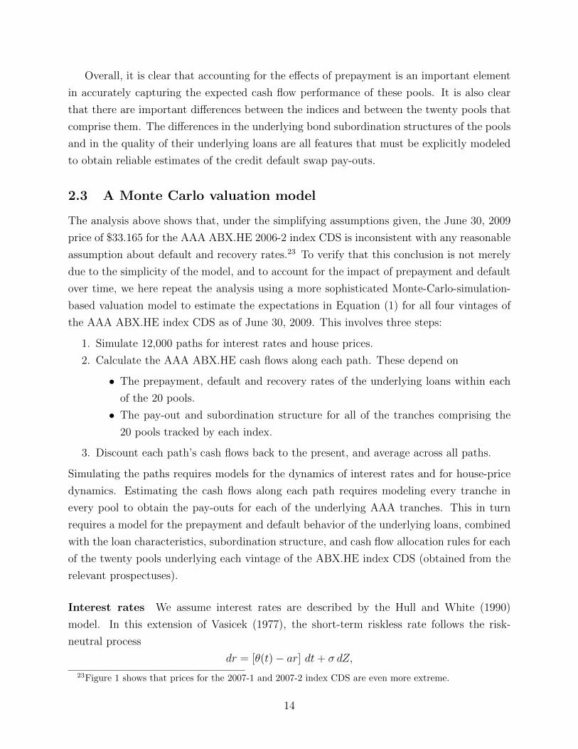
Overall, it is clear that accounting for the effects of prepayment is an important element
in accurately capturing the expected cash flow performance of these pools. It is also clear
that there are important differences between the indices and between the twenty pools that
comprise them. The differences in the underlying bond subordination structures of the pools
and in the quality of their underlying loans are all features that must be explicitly modeled
to obtain reliable estimates of the credit default swap pay-outs.
2.3 A Monte Carlo valuation model
The analysis above shows that, under the simplifying assumptions given, the June 30, 2009
price of $33.165 for the AAA ABX.HE 2006-2 index CDS is inconsistent with any reasonable
assumption about default and recovery rates.23 To verify that this conclusion is not merely
due to the simplicity of the model, and to account for the impact of prepayment and default
over time, we here repeat the analysis using a more sophisticated Monte-Carlo-simulation-
based valuation model to estimate the expectations in Equation (1) for all four vintages of
the AAA ABX.HE index CDS as of June 30, 2009. This involves three steps:
1. Simulate 12,000 paths for interest rates and house prices.
2. Calculate the AAA ABX.HE cash flows along each path. These depend on
• The prepayment, default and recovery rates of the underlying loans within each
of the 20 pools.
• The pay-out and subordination structure for all of the tranches comprising the
20 pools tracked by each index.
3. Discount each path’s cash flows back to the present, and average across all paths.
Simulating the paths requires models for the dynamics of interest rates and for house-price
dynamics. Estimating the cash flows along each path requires modeling every tranche in
every pool to obtain the pay-outs for each of the underlying AAA tranches. This in turn
requires a model for the prepayment and default behavior of the underlying loans, combined
with the loan characteristics, subordination structure, and cash flow allocation rules for each
of the twenty pools underlying each vintage of the ABX.HE index CDS (obtained from the
relevant prospectuses).
Interest rates We assume interest rates are described by the Hull and White (1990)
model. In this extension of Vasicek (1977), the short-term riskless rate follows the risk-
neutral process
dr = [θ(t)− ar] dt+ σ dZ,
23Figure 1 shows that prices for the 2007-1 and 2007-2 index CDS are even more extreme.
14

where the function θ(t) is fitted so that the model matches the yield curve for the U.S. Libor
swap rate on June 30, 2009. Hull and White (1990) show that θ(t) is given by
θ(t) = Ft(0, t) + aF (0, t) +σ2
2a
(1− e−2at
),
where F (0, t) is the continuously compounded forward rate at date 0 for an instantaneous
loan at t. Parameters a and σ were fitted using maximum likelihood, yielding estimates of
0.0552 for a and 0.0107 for σ. For this analysis, we used U.S. Libor yield curve data and
implied caplet volatilities as of June 30, 2009, obtained from Citigroup’s Yieldbook.
House prices We assume that house prices, Ht, follow a geometric Brownian motion,
dHt = θHHt dt+ φHHt dWH,t, (5)
where θH is the expected appreciation in house prices and φH their volatility. Denoting the
flow of rents accruing to the homeowner by qH , after risk-adjustment house prices evolve
according to:
dHt = (rt − qH)Ht dt+ φHHt dWH,t. (6)
We calibrate equation (6) as follows:
qH = 0.025,
φH = 0.12.
This value of qH is consistent with estimates of owner-equivalent rents from the Bureau of
Economic Activity (BEA). We estimate the annualized volatility of housing returns, φH ,
using a long time series of California housing transactions from 1970 to 2008 as a proxy for
the segment of the housing market securitized into the private-label loans that appear in the
ABX.HE pools. These estimates are based on those in Stanton and Wallace (2009), using
418,000 single-family residential transactions in the counties of San Francisco and Alameda,
California, between 1970 and 2008. For simplicity, we assume that house prices and interest
rates are uncorrelated.
Prepayment and default behavior We model the cash flows for the fixed- and adjustable-
rate loans using separately estimated hazard rates for prepayment and default. We estimate
these out-of-sample using a loan-level data set containing 59,290 adjustable-rate mortgages
originated between 2004 and 2007 and 27,826 fixed-rate mortgages originated over the same
15

time frame, all loans of the same type as those underlying the ABX.HE index CDS. These
data were obtained from CTSlink, Bloomberg, and Lewtan ABSNet. The hazards were
estimated using a time-varying-covariate hazard model with a log-logistic baseline hazard
and controls for loan characteristics including the amortization structure, coupon, weighted-
average life, loan-to-value ratios, the balance factor, and indexing (such as the maximum
life-of-loan caps and the periodic interest-rate caps).
We estimate proportional hazard models for the prepayment and default termination
rates for the ARMs and FRMs. The estimated hazard rate is the conditional probability
that a mortgage will terminate given that it has survived up until a given time since origi-
nation. Hazard models comprise two components: 1) a baseline hazard that determines the
termination rates simply as a function of time and 2) shift parameters for the baseline defined
by the time-varying evolution of exogenous determinants of prepayment and default. We fol-
low Schwartz and Torous (1989) and estimate log-logistic proportional hazard specifications
for ARM and FRM prepayment and default rates of the form
π(t) = π0(t)eβν , where (7)
π0(t) =γp(γt)p−1
1 + (γt)p. (8)
The first term on the right-hand side of Equation (7) is the log-logistic baseline hazard,
which increases from zero at the origination date (t = 0) to a maximum at t = (p−1)1/p
γ. This
is shifted by the factor eβν , where β is a vector of parameters and ν a vector of covariates
including the end-of-month difference between the current coupon on the mortgage and
LIBOR, the current loan-to-value ratio of the mortgage, the proportion of the outstanding
balance remaining, and a dummy variable reflecting whether the current month is in the
Spring or Summer (when most home moves occur).
The results of our hazard models are reported in Table 4. As expected, there is a
statistically significant, positive coefficient on the differential between the coupon rate on
the mortgage and the observed swap rate in the estimated prepayment hazard, a statistically
significant, positive coefficient on the loan-to-value ratio of the loan in the default hazard,
and a statistically significant negative effect of the LTV ratio on prepayment. The balance
factor (the proportion of the initial pool still remaining) has a statistically significant negative
effect on prepayment and a positive effect on default. The Summer and Spring indicator
variable does not have a statistically significant effect in either specification.
Valuation results To compare the Monte Carlo valuation procedure with the back-of-the-
envelope model, we here value the four AAA ABX.HE index CDS using the prepayment and
16

Table 4: Loan-level Estimates of the Prepayment and Default Hazards
Adjustable Rate Mortgages Fixed Rate MortgagesCoeff. Est. Std. Err. Coeff. Est. Std. Err.
Prepayment
γ 0.0146∗∗∗ 0.008 0.0154∗∗∗ 0.0018p 1.0609∗∗∗ 0.0167 1.2446∗∗∗ 0.0164Current Coupon minus LIBOR(t) 0.4027∗∗∗ 0.044 0.5576∗∗∗ 0.0436Loan-to-Value Ratio(t) -0.6498∗∗∗ 0.1276 -0.8074∗∗∗ 0.0304Outstanding Balance(t) -0.3443 0.3423 -0.928 0.4952Summer/Spring Indicator Variable 0.2886 0.1362 0.3878∗∗∗ 0.0352
Default
γ 0.0321∗∗∗ 0.0019 0.0086∗∗∗ 0.0009p 1.002∗∗∗ 0.0198 1.0208∗∗∗ 0.0220Current Coupon minus LIBOR(t) 0.425∗∗ 0.1931 0.5376∗∗∗ 0.0468Loan-to-Value Ratio(t) 0.1193∗∗ 0.0523 0.0721 0.0347Outstanding Balance(t) 0.1551∗∗ 0.0862 0.1316∗∗∗ 0.0317Summer/Spring Indicator Variable 0.0006 0.1434 0.0312 0.0397
t statistics in parentheses∗∗ p < 0.05, ∗∗∗ p < 0.01
default models estimated above. We start by simulating 12,000 paths for interest rates and
house prices, using antithetic variates to reduce standard errors (see Glasserman, 2004).24
Along each path, we use the estimated prepayment and default models, together with the
pay-out details for each pool from the prospectus, to determine the cash flows each month.
We discount these back to the present using the simulated path of the risk-free rate, and
average across paths to obtain a Monte Carlo estimate of each security’s NPV.
In performing the valuation as of June 30, 2009, we determine the loan composition
for each of the pools on that date for each deal using data from ABSNet. We then track
the prepayment and default behavior of the fixed- and adjustable- rate loans in each pool
separately. The first panel (OAS=0) of Table 5 shows the net present value (present value
of insurance benefits minus cost of insurance) on June 30, 2009, of the four vintages of AAA
ABX.HE index CDS securities for various assumptions about recovery rates. The results are
again similar to those from the back-of-the-envelope model above. In particular, the NPVs
of all four AAA CDS are negative for every possible recovery rate between 40% and 100%,
and are negative for all recovery rates for three of the four CDS.
24Because we are assuming a constant rate of default, independent of the level of house prices, we do notalso need to simulate the house price process.
17

Table 5: Valuation results for the AAA ABX.HE 2006-1 index CDS, AAA ABX.HE 2006-2index CDS, AAA ABX.HE 2007-1 index CDS, and AAA ABX.HE 2007-2 index CDS
The table shows the net present value per dollar of principal insured for the AAA index for each
of the ABX.HE 2006-1, ABX.HE 2006-2, ABX.HE 2007-1, and ABX.HE 2007-2 index CDS as of
June 30, 2009, given the respective closing prices on that day for each of the indices. The cash
flows for the simulations are based upon empirically estimated hazard rates for prepayment and
default. The hazard rates were estimated using performance data from a large sample of 27,826
fixed rate mortgages and 59,290 adjustable rate mortgages both monitored between 2005 through
2009. The data were obtained from ABSnet.
ValuesRecovery Rates ABX.HE 2006-1 ABX.HE 2006-2 ABX.HE 2007-1 ABX.HE 2007-2
OAS = 0
100% -0.311 -0.670 -0.744 -0.74660% -0.311 -0.643 -0.724 -0.70150% -0.311 -0.607 -0.654 -0.53440% -0.296 -0.559 -0.554 -0.30020% -0.256 -0.383 -0.399 0.0350% -0.198 -0.127 -0.335 0.112
OAS = 50 bp
100% -0.310 -0.670 -0.743 -0.74660% -0.310 -0.646 -0.725 -0.69650% -0.310 -0.615 -0.657 -0.53240% -0.295 -0.572 -0.560 -0.30320% -0.257 -0.418 -0.410 0.0260% -0.202 -0.187 -0.345 0.104
OAS = 150 bp
100% -0.310 -0.670 -0.743 -0.74660% -0.310 -0.652 -0.722 -0.69550% -0.310 -0.626 -0.640 -0.53940% -0.303 -0.591 -0.489 -0.32120% -0.284 -0.472 -0.210 -0.0010% -0.257 -0.282 -0.062 0.082
Quoted Price on June 30, 2009 0.691 0.332 0.258 0.257Premium (Basis points) 18 11 9 76
18

Robustness checks Before taking these results at face value, however, it is important
to note that option-adjusted spreads (OAS) on many securities were widening during this
period.25 For example, Krishnamurthy (2010, Figure 9) shows that OAS for plain-vanilla
mortgage-backed securities were close to zero throughout 2007, but then rose steadily to
almost 1.5% by early 2009, before falling again to about 0.5% by the middle of 2009. We
need to rule out the possibility that our results are merely a symptom of this market-wide
phenomenon.26 In the second and third panels of Table 5, we therefore repeat the analysis
in the first panel, but this time using an OAS of 0.5% and 1.5%, respectively.27 While the
numbers change slightly, the overall conclusion remains identical: the NPVs are negative for
almost every possible recovery rate.
Because our estimated default model includes house prices as one of the explanatory
variables, it will automatically result in higher default rates when house prices fall, as they
did prior to June 2009. However, as an additional robustness check, we repeated all of
our valuation results using the same model as above, but multiplying the estimated default
hazard rates by two. The results are shown in Table 6, and do not materially change any
of our conclusions. Overall, the Monte Carlo results support the conclusion of the back-
of-the-envelope model above: all of the ABX.HE index CDS are mispriced given expected
default risk, due primarily to the large up-front payments for the insurance based upon the
quoted prices from Markit.
3 Empirical analysis of ABX.HE index CDS price changes
The results from Section 2 suggest that, whatever is driving AAA ABX.HE index CDS
prices, it is not just expectations of future default rates on the underlying mortgages. We
here investigate in more detail the empirical determinants of changes in the quoted prices
for the AAA ABX.HE index CDS. The goal of this investigation is to answer two questions.
First, even though we know ABX.HE index CDS prices do not solely reflect expectations of
future default behavior, are they related at all to news about the credit performance of the
referenced basket of subprime obligations? Second, given that default behavior cannot fully
explain observed prices, what other variables are empirically significant?
25To match model and market prices for mortgage-related securities, it is standard practice to add a fixedspread, the Option-Adjusted Spread, to the risk-free rate when discounting projected cash flows along eachpath. For details, see Hayre (2001).
26We thank the referee for this suggestion.27In other words, when doing the valuation, we discount the cash flows at (r + OAS) rather than just r.
19
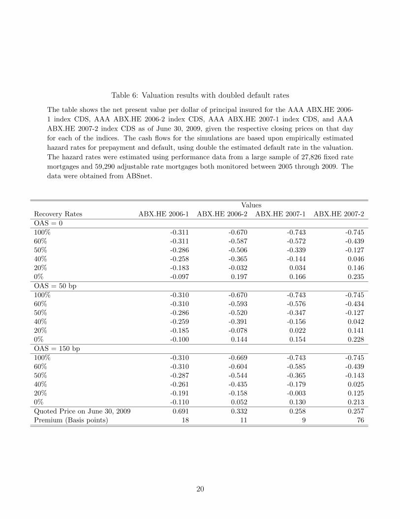
Table 6: Valuation results with doubled default rates
The table shows the net present value per dollar of principal insured for the AAA ABX.HE 2006-
1 index CDS, AAA ABX.HE 2006-2 index CDS, AAA ABX.HE 2007-1 index CDS, and AAA
ABX.HE 2007-2 index CDS as of June 30, 2009, given the respective closing prices on that day
for each of the indices. The cash flows for the simulations are based upon empirically estimated
hazard rates for prepayment and default, using double the estimated default rate in the valuation.
The hazard rates were estimated using performance data from a large sample of 27,826 fixed rate
mortgages and 59,290 adjustable rate mortgages both monitored between 2005 through 2009. The
data were obtained from ABSnet.
ValuesRecovery Rates ABX.HE 2006-1 ABX.HE 2006-2 ABX.HE 2007-1 ABX.HE 2007-2
OAS = 0
100% -0.311 -0.670 -0.743 -0.74560% -0.311 -0.587 -0.572 -0.43950% -0.286 -0.506 -0.339 -0.12740% -0.258 -0.365 -0.144 0.04620% -0.183 -0.032 0.034 0.1460% -0.097 0.197 0.166 0.235
OAS = 50 bp
100% -0.310 -0.670 -0.743 -0.74560% -0.310 -0.593 -0.576 -0.43450% -0.286 -0.520 -0.347 -0.12740% -0.259 -0.391 -0.156 0.04220% -0.185 -0.078 0.022 0.1410% -0.100 0.144 0.154 0.228
OAS = 150 bp
100% -0.310 -0.669 -0.743 -0.74560% -0.310 -0.604 -0.585 -0.43950% -0.287 -0.544 -0.365 -0.14340% -0.261 -0.435 -0.179 0.02520% -0.191 -0.158 -0.003 0.1250% -0.110 0.052 0.130 0.213
Quoted Price on June 30, 2009 0.691 0.332 0.258 0.257Premium (Basis points) 18 11 9 76
20

3.1 Empirical specification and data description
To explore the determinants of AAA ABX.HE index CDS price changes, we regress the
monthly percentage changes in the quoted price of the respective AAA ABX.HE index CDS
for 2006-1, 2006-2, 2007-1, and 2007-2, on a selection of potential explanatory variables. The
regression specification is:
∆ABXAAAit = βAAA0 + βAAA1 ∆ABXi,t−1 + +
∑βAAAl ∆Xi,Creditlt
+∑
βAAAl ∆Xi,Shortlt +∑
βAAAl ∆Xi,Controllt + εAAAit , (9)
where ∆ indicates percentage changes, and the right hand side variables control for the credit
performance of the underlying mortgages, the short-sales ratio of firms in mortgage-related
industries, repo rates, and various controls. We now discuss the variables and the data used
in more detail.
ABX.HE prices: The AAA ABX.HE index CDS prices, ABXit, used in our empirical
analysis are as reported to the market by Markit Group Ltd., who report daily trading
prices. We compute the monthly percentage changes in the AAA ABX.HE index CDS
quoted prices using the last quoted price each month. This reporting frequency matches the
end-of-month reporting frequency of the mortgage performance data.
Mortgage credit and prepayment performance: To examine the significance of changes
in credit behavior for the ABX.HE prices, we assemble loan performance information for each
of the subprime residential mortgage-backed security pools referenced by the four trading
ABX.HE index CDS. The performance data, obtained from Bloomberg and Lewtan ABSNet,
include the monthly rates of delinquency, foreclosure, Real Estate Owned,28 and prepayment.
Table 7 reports the time-series average pool-level credit and prepayment performance by vin-
tage. As shown in the table, the average delinquency rates in the 2006-1 and 2006-2 AAA
ABX.HE index CDS pools are higher than those in the 2007-1 and 2007-2 pools, but the
average foreclosure rates and serious delinquency rates are lower. The maximum rates of
foreclosure and loss are also higher for the later vintage pools. As is clear from the standard
deviations and the minimum and maximum values of all the performance characteristics,
there is considerable variability in the monthly realized credit experience across the twenty
deals in each AAA ABX.HE vintage. The average monthly prepayment rate is about 2.3%
for the early vintage pools and about 1.5% for the later vintage pools. The prepayment rate
28This is the dollar value of housing collateral held by the trust after the foreclosure auction.
21

is also quite heterogeneous, particularly in the 2006 vintages pools, which experienced very
significant decreases in interest rates followed by large decreases in house prices. To avoid
having too many explanatory variables, in our regressions we use a single aggregate credit
measure, defined as the sum of the 30-, 60-, and 90-day delinquency, foreclosure, Real Estate
Owned, and loss rates.
Short-sales data: Based on Froot (2001), who found limited capital in the reinsurance
market to be the most likely explanation for the fact that prices for catastrophe insurance
often exceed seven times expected losses, a candidate explanation for the pricing anomalies
described above is lack of capital behind the provision of mortgage-backed-security insurance
via the sale of ABX.HE index CDS. This explanation is not implausible in this market, given
the size of the notional outstanding combined with the fact that, while many institutions are
natural demanders of insurance against mortgage default, very few are natural suppliers of
such insurance. The impact of such capital constraints will vary with shifts in the demand
for insurance.
Since there was no functioning clearinghouse for CDS contracts until recently, we proxy
for insurance demand by looking at measures of short selling in the investment-banking
sector. We follow prior authors (see Lamont and Stein, 2004; Fishman, Hong, and Kubik,
2007; Jones and Lamont, 2002) in the use of the value-weighted short-interest ratio (the
market value of shares sold short, divided by the average daily trading volume). The short-
interest ratio is a measure of how long it would take short sellers, in days, to cover their entire
positions if the price of a stock began to rise. A higher short-interest ratio is usually viewed
by market participants as a bearish signal about a specific stock, and higher ratios have been
found to be associated with other measures of demand pressure for shorting, such as high
premia paid to borrow the stock.29 We obtain monthly data for the short-interest ratio for
publicly traded investment banks from Bloomberg and Shortsqueeze.com from January 2006
to July 2010.
Repo market conditions: Gorton (2008a,b) and Gorton and Metrick (2009) argue that
many of the financial problems observed during 2007–2009 were caused by failure of the repo
market. We therefore include in our regression monthly percentage changes in the overnight
repo rate and in the spread between three-month LIBOR and the overnight index swap (OIS)
rate, downloaded from Bloomberg. Gorton and Metrick (2009) argue that the LIBOR-OIS
spread is a measure of counterparty risk in the interbank lending system.30 A higher value
29See, for example, Lamont and Stein (2004), Jones and Lamont (2002), and Dechow, Hutton, Muelbroek,and Sloan (2001)
30The OIS is a fixed-to-floating interest rate swap where the periodic floating rate of the swap is tied to
22

Table 7: Summary Statistics for the the Pool-level Default, Prepayment, and Loss Perfor-mance Measures in the 2006 and 2007 Vintage AAA ABX.HE index CDS, Using PerformanceData from June 19, 2007 to July 30, 2010.
The table presents the summary statistics for the percentage of the overall outstanding mortgage
collateral that was 30-days delinquent, 60-days delinquent, 90-days delinquent, in foreclosure, lost,
or held as Real Estate Owned, and the thirty-day prepayment rate for the Markit AAA ABX.HE
2006-1 index CDS, AAA ABX.HE 2006-2 index CDS, AAA ABX.HE 2007-1 index CDS, AAA
ABX.HE 2007-2 index CDS pools. We report the summary statistics for the period July, 2007
through July, 2010 (the same period tracked in the panel regressions).
Mean Standard Deviation Minimum Maximum
ABX.HE-2006-1
30 Day Prepayment Rate (%) 2.4 0.9 1.0 5.030 Day Delinquency Rate (%) 4.0 1.4 0.1 5.960 Day Delinquency Rate (%) 2.2 1.1 0.0 3.990 Day Delinquency Rate (%) 5.5 4.9 0.0 15.1Foreclosure Rate (%) 10.2 6.7 0.0 18.4Loss Rate (%) 5.8 3.8 0.0 11.4REO Rate (%) 4.9 3.9 0.0 11.7
ABX.HE-2006-2
30 Day Prepayment Rate (%) 2.2 0.7 0.8 3.430 Day Delinquency Rate (%) 4.2 1.6 0.1 6.360 Day Delinquency Rate (%) 2.3 1.1 0.0 3.890 Day Delinquency Rate (%) 5.5 5.2 0.0 16.3Foreclosure Rate (%) 11.3 8.0 0.0 21.6Loss Rate (%) 7.5 5.1 0.1 15.3REO Rate (%) 5.0 4.1 0.0 12.0
ABX.HE-2007-1
30 Day Prepayment Rate (%) 1.6 0.5 0.3 2.530 Day Delinquency Rate (%) 4.7 1.4 0.0 6.960 Day Delinquency Rate (%) 2.9 1.1 0.0 4.790 Day Delinquency Rate (%) 9.1 7.9 0.0 23.2Foreclosure Rate (%) 12.6 7.2 0.0 20.3Loss Rate (%) 7.5 5.7 0.0 16.8REO Rate (%) 5.0 3.3 0.0 9.6
ABX.HE-2007-1
30 Day Prepayment Rate (%) 1.4 0.5 0.3 2.430 Day Delinquency Rate (%) 5.0 1.7 0.0 7.460 Day Delinquency Rate (%) 3.0 1.3 0.0 4.790 Day Delinquency Rate (%) 8.8 7.2 0.0 21.3Foreclosure Rate (%) 12.9 7.5 0.0 21.4Loss Rate (%) 7.5 6.5 0.0 18.6REO Rate (%) 4.2 2.8 0.0 8.0
23

of this spread is an indication of a decreased willingness to lend by major banks, while a
lower spread indicates lower concerns about counterparty risk. Historically, this spread has
been around 10 basis points. However, on October 10, 2008, the spread spiked to all-time
high of 366 basis points.
House price performance: House prices are an important factor influencing future de-
fault rates. We collect the same data that are available to market participants: the monthly
repeat-sales house-price index for the United States, available from the Office of Housing
Enterprise Oversight (OFHEO, now the Federal Housing Finance Agency, FHFA). Since the
geographic coverage of the loans in the pools is diversified across the states, the national
index is the best representation of the systemic house-price-risk exposure of the pools.
Additional market control variables: We also consider the following market controls:
• Monthly percent changes in the S&P volatility index, VIX, downloaded from Datastream.
VIX is calculated from market prices of CBOE-traded options on the S&P 500 Index,
and is often referred to as the market’s “fear gauge” (see Whaley, 2000). Other studies
(see, for example, Longstaff and Myers, 2009) have used VIX as a measure of the
market’s perception of risk. It thus serves as a measure of potential hedging demand
by market participants.
• Monthly changes in the ten-year constant-maturity Treasury rate, CMT10, obtained
from Datastream. Since the ABX.HE index CDS share the same maturity as the
underlying subprime-mortgage collateral, the effects of discounting should be important
to their values.
• Monthly changes in the slope of the constant-maturity yield curve, slope. This is
calculated as the difference between the ten-year and three-month yields, obtained
from Datastream. The slope of the yield curve is a measure of expected future growth
in the economy, which would presumably affect the demand for housing, and thus
mortgage refinancing and default rates.
• Monthly S&P 500 returns, obtained from Datastream. This measure is included fol-
lowing Longstaff (2010), who finds a positive relation between asset-backed index CDS,
such as the ABX.HE index CDS and the CMBX index CDS, and market returns.
the geometric average of an overnight index, such as the federal funds rate, over every day of the contractualloan payment period. The fixed leg of the swap is the expected average of the overnight federal funds rateover the term of the contract. Since principal does not change hands with these swaps, OIS contracts do nothave significant credit risk exposure.
24

3.2 Results
Column (1) of Table 8 reports results for a fixed-effects panel regressions of changes in AAA
ABX.HE index CDS prices on the variables described above. A test of serial correlation
using the method described in Wooldridge (2002, pp. 282–283) shows that there is significant
serial correlation in the residuals, so all t-statistics are calculated allowing for AR(1) errors,
following Baltagi and Wu (1999).
Surprisingly, the coefficient on the credit variable, while of the expected sign, is econom-
ically small and statistically indistinguishable from zero. Column (2) of Table 8 includes an
additional lag of the credit variable. This time, while the coefficient on the lagged variable
is now significantly negative, the contemporaneous coefficient is again insignificantly differ-
ent from zero, and now of the wrong sign. By contrast, the investment bank short-interest
ratio has a statistically significant negative effect on AAA ABX.HE price changes in both
specifications, hence a positive relation with the cost of insurance. This result suggests that,
similar to the findings of Froot (2001) in the catastrophe insurance market, the price of ABS
insurance moves with supply and demand imbalances related to short-selling the stocks of
investment banks. Since buying AAA ABX.HE index CDS is roughly equivalent to short-
ing the mortgage market or firms with subprime residential mortgage exposure, it appears
that the supply and demand imbalances in the market for shorting the stocks of firms with
subprime mortgage risk positively “spilled over” into the AAA ABX.HE market during this
period. This spill-over effect drove up the cost of insuring AAA residential mortgage-backed
securities, or alternatively, the cost of building up short positions against key mortgage
market participants.
As shown in Table 8, S&P 500 returns are positively associated with shocks to the
quoted ABX.HE prices, so, in line with intuition, the cost of insurance falls as the S&P rises.
Changes in the level of interest rates have a positive coefficient, i.e., a negative effect on the
cost of the insurance. Housing returns have little effect, appearing insignificantly in every
specification. While somewhat surprising, this result may be the result of limitations with
the available indices for measuring house price fluctuations, rather than an indication that
shocks to housing prices did not affect the costs of insuring AAA residential mortgage-backed
securities bonds through the AAA ABX.HE CDS. Different from Gorton and Metrick (2009),
the changes in the repo rate and in the LIBOR-OIS spread are not significantly associated
with changes in AAA ABX.HE index CDS quoted prices.31
Overall, these results suggest that the short-interest imbalance channel had a larger
economic effect on ABX.HE index CDS returns than did credit events on the mortgages over
31These results are unchanged if we include only one of the LIBOR-OIS spread or the repo rate in theregressions.
25

Table 8: Regressions for monthly percentage changes in the quoted prices of the 2006 and 2007Vintage AAA ABX.HE index CDS, using data from June 19, 2007 to July 30, 2010. t-statisticsrobust to AR(1) errors are calculated according to Baltagi and Wu (1999).
(1) (2)% Price Change % Price Change
Lag 1 ∆ ABX Quoted Price Changes -0.224∗∗∗ -0.256∗∗∗
(-2.81) (-3.29)
∆ Credit -0.00945 0.0227(-0.91) (1.43)
∆ Prepayment -0.0351 -0.0265(-1.23) (-0.95)
∆ S&P 1.803∗∗ 2.601∗∗∗
(2.05) (2.83)
∆ House Price Returns -28.48 -20.46(-0.80) (-0.58)
∆ Bank Ratio -0.500∗∗∗ -0.544∗∗∗
(-3.44) (-3.83)
∆ LIBOR minus OIS 0.0615 0.0291(0.24) (0.12)
∆ Repo Rate -0.0120 0.00744(-0.28) (0.17)
∆ 10-year Treasury 0.533∗∗∗ 0.392∗∗
(3.30) (2.35)
∆ Slope (10-year CMT minus 3-month Rate) 0.0178 0.0402(0.32) (0.73)
∆ VIX Rate -0.0112 0.123(-0.06) (0.62)
Lag 1 ∆ Credit -0.0432∗∗∗
(-2.59)
Constant -0.0220 -0.00400(-1.46) (-0.24)
Observations 127 127R2 0.4519 0.4792
t statistics in parentheses∗ p < 0.10, ∗∗ p < 0.05, ∗∗∗ p < 0.01
26

this time period. Other important factors affecting the prices of the AAA ABX.HE index
CDS include the level of interest rates and movements in the stock market.
4 Conclusions
Despite the rapid growth of the ABX.HE index CDS market, and the focus of regulators on
banks using CDS market prices as the basis for marking their portfolios to market, we find
that market prices for AAA ABX.HE index CDS at the peak of the financial crisis in June
2009 are inconsistent with any reasonable assumptions for future default rates. Although
we find that percentage changes in CDS prices are correlated with changes in the realized
foreclosure rates of the underlying loans, we also find that changes in short-sale imbalances in
the equity markets of the publicly traded investment banks have a statistically significant and
large economic impact on CDS prices. Because our short-sale activity measure is a proxy for
demand imbalances in the market for mortgage default insurance, the relative importance
of its correlation with CDS price dynamics suggests that the practice of using the AAA
ABX.HE index CDS to value subprime mortgage portfolios is quite problematic. Indeed, if
we use AAA ABX.HE index CDS prices to mark to market all bonds rated AAA on June 30,
2009 (a total of 10,754 AAA bonds) by multiplying the outstanding principal balances on
the bonds by the relevant AAA ABX.HE index CDS price (taken as a percentage), we find
that, by June 2009, the aggregate write-down for these AAA bonds (which have experienced
trivial principal losses to date) was $90.8 billion.32
Besides their immediate policy implications in the mortgage market, our findings add to
a growing body of research documenting how limits to arbitrage (see Shleifer and Vishny,
1997) and capital constraints can allow prices in many markets to i. diverge significantly
from fundamentals; and ii. move with variables unrelated to fundamentals. Several recent
papers, including Brunnermeier and Pedersen (2009), Duffie (2010), Ashcraft, Garleanu,
and Pedersen (2010), and Garleanu and Pedersen (2011), show in particular that frictions
such as slow-moving capital or margin constraints may cause substantial mispricings and
deviations from the law of one price, especially during financial crises. Empirical evidence
of these effects includes Gabaix, Krishnamurthy, and Vigneron (2007), who find that the
idiosyncratic risk of homeowner prepayment (which must net to zero in aggregate) is priced
in the mortgage-backed securities market. They attribute this to limits of arbitrage in the
market, caused by the marginal investor being a specialized arbitrageur with limited capital,
32Bonds issued prior to January 2006 were marked to market using the 2006-1 vintage ABX.HE indexCDS. Bonds issued between January and June of 2006 were marked to market using the 2006-2 vintageABX.HE, and so on. All bonds issued after June 2007 were marked to market using the 2007-2 ABX index.
27

rather than a diversified representative investor. Krishnamurthy (2010) discusses mispricings
between Treasury rates and 30-year fixed-for-floating (LIBOR) interest rate swap rates. Bai
and Collin-Dufresne (2010) examine mispricings between corporate bonds and CDS written
on the same company. Finally, Froot (2001) studies mispricings in the market for catastrophe
insurance. In this market, losses due to natural disasters are both large and approximately
uncorrelated with the state of the overall economy, so we should expect to see large demand
for insurance, especially against catastrophic losses, and this insurance should be priced
roughly at the level of expected losses. In contrast, Froot (2001) documents that protection
tends to be relatively limited, and is always priced well above the level of expected losses,
sometimes as much as seven times as high. He concludes, supported by statements by players
in the industry such as National Indemnity,33 that this is caused by the absence of sufficient
capital in the reinsurance market. Our results suggest that similar dislocations may exist in
the ABX.HE market.
Finally, our findings contribute to the growing debate concerning the wisdom of mov-
ing regulated financial institutions, especially those holding large investment portfolios of
loans, to a full mark-to-market accounting system. A number of recent papers (see, for
example, Brunnermeier and Pedersen, 2009; Shleifer and Vishny, 2009; Allen and Carletti,
2008; Plantin, Sapra, and Shin, 2008) have analyzed the link between the funding liquidity
and market liquidity of financial institutions, and have found this to be an important source
of systemic risk with the potential to generate destabilizing liquidity spirals. Although the
mechanisms differ in these papers, mark-to-market accounting further exacerbates these ef-
fects by inducing potentially excessive and artificial volatility into accounting valuations,
thus distorting regulatory capital requirements and the timing of liquidations (see Allen
and Carletti, 2008; Plantin et al., 2008; Freixas and Tsomocos, 2004) and increasing the
likelihood that rational trading will be based on irrelevant information (see Gorton, He,
and Huang, 2006). Our results, showing that the ABX.HE index CDS prices appear to be
only very weakly related to the performance of the underlying mortgages, strongly reinforce
this concern, and suggest that the use of these CDS for the fair-market valuation of mort-
gage loans held in the portfolios of financial institutions, or for loans on the trading books of
these institutions, is likely to lead to important distortions.34 These distortions could lead to
33National Indemnity, a subsidiary of Berkshire Hathaway, is one of the largest reinsurance companies.34In May, 2010, the Financial Accounting Standards Board (FASB) proposed to expand the use of mark-to-
market accounting from just loans intended for sale to also include loans that financial institutions planned tohold to maturity (see U.S. Banker, “FASB Mark-to-Market Plan Could Have a Seismic Impact,” by HeatherLandy, June, 2010). As the result of these proposals, “...Lenders including Bank of America Corp., based inCharlotte, North Carolina, and San Francisco-based Wells Fargo already report the fair value of their loansin the footnotes of their quarterly reports to regulators. Reporting changes through other comprehensiveincome could cause swings of billions of dollars in their book values...” (see Michael J. Moore, “FASB Backs
28

bank insolvency and could affect new loan origination strategies or the liquidation strategies
implemented for existing mortgage loans.35
Off Fair-Value of Loans Proposal After Opposition,” Bloomberg.com, January 25, 2011).35Bhat, Frankel, and Martin (2010) find empirical evidence that AAA ABX.HE 2006-1 index CDS price
dynamics were positively associated with sales of non-agency mortgage backed securities by regulated U.S.financial institutions and this correlation dissipated once FASB eased the mark-to-market rules temporarilyon April 2, 2009.
29

References
Allen, F., and E. Carletti, 2008, Mark-to-market accounting and liquidity pricing, Journal
of Accounting and Economics 45, 358–378.
Ashcraft, A., N. Garleanu, and L. H. Pedersen, 2010, Two monetary tools: Interest rates
and haircuts, Working paper, U.C. Berkeley.
Bai, J., and P. Collin-Dufresne, 2010, The determinants of the CDS-bond basis during the
financial crisis of 2007–2009, Working paper, Columbia University.
Baltagi, B., and P. Wu, 1999, Unequally spaced panel data regressions with AR(1) distur-
bances, Econometric Theory 15, 814–823.
Bank of England, 2008, Financial stability report, Working paper 23, Bank of England.
Bhat, G., R. Frankel, and X. Martin, 2010, Panacea, Pandora’s box, or placebo: Feedback
in bank holdings of mortgage-backed securities and fair-value accounting, Working paper,
Washington University in St. Louis.
Bridewell, D. A., 1938, The Federal Home Loan Bank Board and its Agencies: A History
of the Facts Surrounding the Passage of the Creating Legislation, the Establishment and
Organization of the Federal Home Loan Bank Board and the Bank System, the Savings
and Loan System, the Home Owners’ Loan Corporation, and the Federal Savings and
Loan Insurance Corporation (Federal Home Loan Bank Board, Washington, D.C.).
Brunnermeier, M., and L. Pedersen, 2009, Market liquidity and funding liquidity, Review of
Financial Studies 22, 2201–2199.
Case, K. E., and R. J. Shiller, 1989, The efficiency of the market for single family homes,
American Economic Review 79, 125–137.
Davidson, A., A. Sanders, L.-L. Wolff, and A. Ching, 2003, Securitization: Stucturing and
Investment Analysis (Wiley, New York, NY).
Dechow, P., A. P. Hutton, L. Muelbroek, and R. Sloan, 2001, Short-sellers, fundamental
analysis and stock returns, Journal of Financial Economics 66, 271–300.
Driessen, J., and O. Van Hemert, 2011, Pricing of commercial real estate securities during
the 2007–2009 financial crisis, Working paper, NYU.
Duffie, D., 2010, Asset price dynamics with slow-moving capital, Working paper, Stanford
University, Forthcoming, Journal of Finance.
Economist, March 8, 2008, Valuing securities: Don’t mark to Markit, Economist 42.
Fender, I., and P. Hoerdahl, 2008, Overview: A cautious return of risk tolerance, BIS Quar-
terly Review 1–16.
Fender, I., and M. Scheicher, 2008, The ABX: How do the markets price subprime mortgage
risk?, BIS Quarterly Review 67–81.
30
Fishman, T., H. Hong, and J. D. Kubik, 2007, Do arbitrageurs amplify economic shocks,
Working paper, Princeton University.
Freixas, X., and D. P. Tsomocos, 2004, Book vs. fair value accounting in banking and
intertemporal smoothing, Working paper, Universitat Pompeu Fabra.
Froot, K. A., 2001, The market for catastrophe risk: A clinical examination, Journal of
Financial Economics 60, 529–571.
Gabaix, X., A. Krishnamurthy, and O. Vigneron, 2007, Limits of arbitrage: Theory and
evidence from the mortgage-backed securities market, Journal of Finance 62, 557–595.
Garleanu, N., and L. H. Pedersen, 2011, Margin-based asset pricing and deviations from the
law of one price, Working paper, U.C. Berkeley, forthcoming, Review of Financial Studies.
Glasserman, P., 2004, Monte Carlo Methods in Financial Engineering , number 53 in Appli-
cations of Mathematics (Springer, New York).
Goldman Sachs, 2010, Valuation and pricing related to transactions with AIG, Technical
Report.
Gorton, G., 2008a, Information, liquidity, and the panic of 2007, American Economic Review,
Papers and Proceedings, forthcoming.
Gorton, G., 2008b, The panic of 2007, Working paper, Yale School of Management and
NBER.
Gorton, G., P. He, and L. Huang, 2006, Asset prices when agents are marked-to-market,
NBER working paper series, National Bureau of Economic Research.
Gorton, G., and A. Metrick, 2009, Securitized banking and the run on repo, Working paper,
Yale University.
Harriss, C. L., 1951, History and Policies of the Home Owners’ Loan Corporation (National
Bureau of Economic Research, New York).
Hayre, L., ed., 2001, Salomon Smith Barney Guide to Mortgage-Backed and Asset-Backed
Securities (John Wiley, New York).
Hull, J., and A. White, 1990, Pricing interest rate derivative securities, Review of Financial
Studies 3, 573–592.
Jones, C. M., and O. A. Lamont, 2002, Short-sale constraints and stock returns, Journal of
Financial Economics 66, 207–239.
Kazarian, D., D. Mingelgrin, S. Risa, V. Huang, G. Ciampini, and O. Brav, 2005, ABS credit
default swaps — a primer, Fixed income research, Lehman Brothers.
Kelly, K., December 14, 2007, How Goldman won big on the mortgage meltdown, The Wall
Street Journal .
Kinsey, M. A., 1998, Evaluating the capital adequacy of Freddie Mac and Fannie Mae,
Secondary Mortgage Markets 15, 47–53.
31

Krishnamurthy, A., 2010, How debt markets have malfunctioned in the crisis, Journal of
Economic Perspectives 24, 3–28.
Lamont, O. A., and J. C. Stein, 2004, Aggregate short interest and market valuations,
American Economic Review, Papers and Proceedings 94, 29–32.
Lewis, M., February 16, 2008, What does Goldman know that we don’t?, Bloomberg.com .
Logan, B., 2008, The ABX index: A pricing conundrum, Credit .
Longstaff, F., and B. Myers, 2009, How does the market value toxic assets?, Working paper,
University of California, Los Angeles.
Longstaff, F. A., 2010, The subprime credit crisis and contagion in financial markets, Journal
of Financial Economics 97, 436–450.
Lowell, L., 2008, Viewpoint: Those who bury history are doomed to repeat it, HousingWire
April 9.
Mackintosh, J., January 15, 2008, Record profits for fund shorting subprime, The Financial
Times .
Ng, S., and C. Mollenkamp, 2010, Goldman details its valuations with AIG, The Wall Street
Journal .
Ng, S., C. Mollenkamp, and S. Patterson, 2007, A ‘Subprime’ gauge in many ways, The Wall
Street Journal C1.
Plantin, G., H. Sapra, and H. S. Shin, 2008, Marking-to-market: Panacea or Pandora’s box?,
Journal of Accounting Research 46, 435–460.
Rose, J. D., 2010, The incredible HOLC? Mortgage relief during the Great Depression,
Working paper, Federal Reserve Board.
Saulnier, R. J., 1950, Urban mortgage loan experience of life insurance companies, 1920–46,
in Urban Mortgage Lending by Life Insurance Companies , chapter 6, 79–106 (NBER).
Schwartz, E. S., and W. N. Torous, 1989, Prepayment and the valuation of mortgage-backed
securities, Journal of Finance 44, 375–392.
Senior Supervisors Group, 2008, Observations on risk management practices during the
recent market turbulence, Technical report, Senior Supervisors Group.
Shleifer, A., and R. Vishny, 2009, Unstable banking, Journal of Financial Economics 97,
306–318.
Shleifer, A., and R. W. Vishny, 1997, The limits of arbitrage, Journal of Finance 36, 35–55.
Snowden, K. A., 2006, Mortgage foreclosures and delinquencies: 1926–1979, in S. B. Carter,
S. S. Gartner, M. R. Haines, A. L. Olmstead, R. Sutch, and G. Wright, eds., Historical
Statistics of the United States, Earliest Times to the Present: Millennial Edition (Cam-
bridge University Press, New York, NY), Table Dc1255–1270.
32

Standard and Poor’s, 1993, Texas default study confirms loan-loss assumptions, Credit Com-
ments February, 7–9.
Stanton, R., and N. Wallace, 2009, Dynamic house price indices: Foundations for a new
estimator, Working paper, U.C. Berkeley.
Vasicek, O. A., 1977, An equilibrium characterization of the term structure, Journal of
Financial Economics 5, 177–188.
Whaley, R. E., 2000, The investor fear gauge, Journal of Portfolio Management 26, 12–17.
Wheelock, D. C., 2008a, Changing the rules: State mortgage foreclosure moratoria during
the Great Depression, Federal Reserve Bank of St. Louis Review 90, 569–583.
Wheelock, D. C., 2008b, The Federal response to home mortgage distress: Lessons from the
Great Depression, Federal Reserve Bank of St. Louis Review 90, 133–148.
Wood, D., 2008, The blame game, Risk Magazine 21, 54–56.
Wooldridge, J. M., 2002, Econometric Analysis of Cross Section and Panel Data (MIT Press,
Cambridge, MA).
Zuckerman, G., January 15, 2008, Trader made billions on subprime, Online.WSJ.com .
33