The Berkovich Ramification Locus:Structure and Applications

Xander FaberUniversity of Hawai‘i at Manoa

ICERM Workshop on Complex and p-adic Dynamics

www.math.hawaii.edu/∼xander/lectures/ICERM BerkTalk.pdf

February 14, 2012

Itinerary

• Analytic P1 and Rational Functions

• The Berkovich Ramification Locus

• Examples of Ramification Loci

• Structure Theorems

• Examples Redux

• Applications

• Final Thoughts . . .

Notation

Cp completion of Qp, normalized with |p| = 1/p

Fp residue field of Cp

D(a, r) = {x ∈ Cp : |x− a| ≤ r} “closed disk”

D(a, r)− = {x ∈ Cp : |x− a| < r} “open disk"

P1 Berkovich Cp-analytic space associated to P1

Note: When p is large, you may think of Puiseux series instead — i.e.,the completion of an algebraic closure of C((t)).

The Analytic Space P1

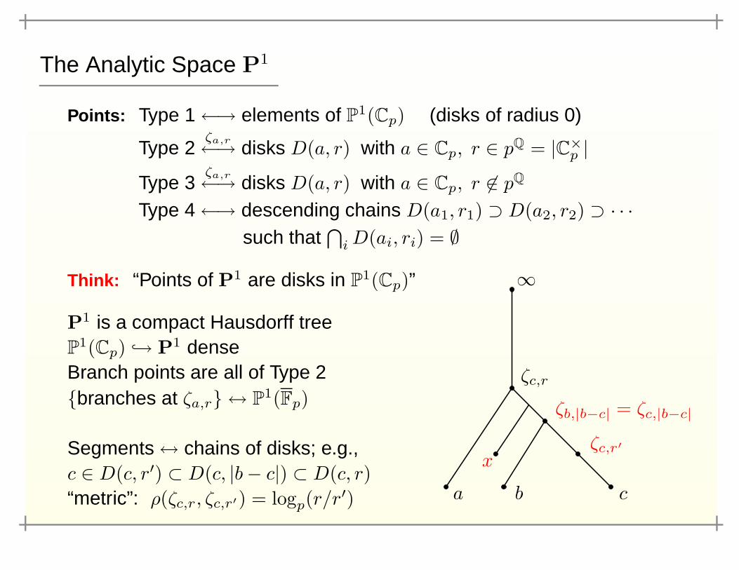
Points: Type 1←→ elements of P1(Cp) (disks of radius 0)

Type 2ζa,r←→ disks D(a, r) with a ∈ Cp, r ∈ pQ = |C×

p |Type 3

ζa,r←→ disks D(a, r) with a ∈ Cp, r �∈ pQ

Type 4←→ descending chains D(a1, r1) ⊃ D(a2, r2) ⊃ · · ·such that

⋂iD(ai, ri) = ∅

Think: “Points of P1 are disks in P1(Cp)”

P1 is a compact Hausdorff treeP1(Cp) ↪→ P1 denseBranch points are all of Type 2{branches at ζa,r} ↔ P1(Fp)

Segments↔ chains of disks; e.g.,c ∈ D(c, r′) ⊂ D(c, |b− c|) ⊂ D(c, r)“metric”: ρ(ζc,r, ζc,r′) = logp(r/r

′)

∞

ζc,r

a b c

x

ζb,|b−c| = ζc,|b−c|

ζc,r′

Rational Functions

ϕ : P1 → P1 nonconstant rational function defined over Cp

� ϕ : P1 → P1 functorial extension to P1

On Type 1 Points: agrees with ϕ : P1(Cp)→ P1(Cp)

On Type 2, 3 Points:

If ϕ(D(a, r) ) = D(b, s), then ϕ(ζa,r) = ζb,s.If ϕ(D(a, r) ) = P1(Cp) �D(b, s)−, then ϕ(ζa,r) = ζb,s.

Not a complete description . . . can also have ϕ(D(a, r) ) = P1(Cp)

On Type 4 Points: Take limits of Type 2,3 points.

Think: “If points of P1 are disks in P1(Cp),then ϕ keeps track of mapping properties of disks.”

The Berkovich Ramification Locus

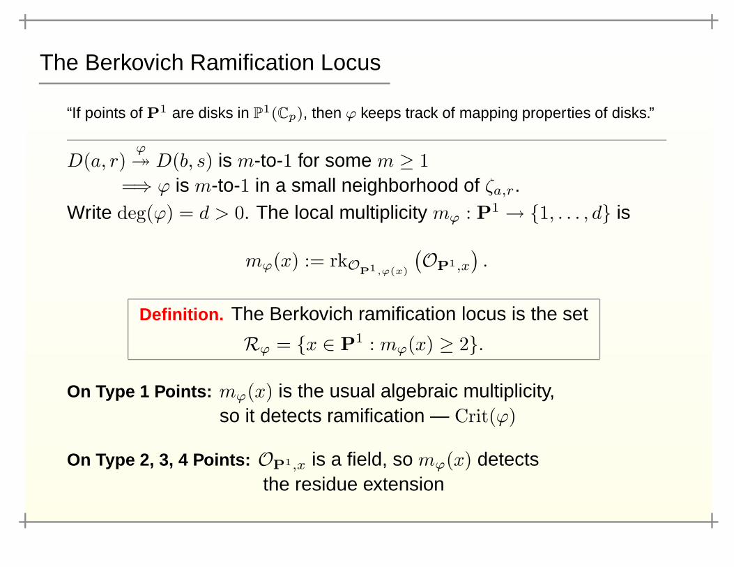
“If points of P1 are disks in P1(Cp), then ϕ keeps track of mapping properties of disks.”

D(a, r)ϕ� D(b, s) is m-to-1 for some m ≥ 1

=⇒ ϕ is m-to-1 in a small neighborhood of ζa,r.Write deg(ϕ) = d > 0. The local multiplicity mϕ : P1 → {1, . . . , d} is

mϕ(x) := rkOP1,ϕ(x)

(OP1,x

).

Definition. The Berkovich ramification locus is the set

Rϕ = {x ∈ P1 : mϕ(x) ≥ 2}.

On Type 1 Points: mϕ(x) is the usual algebraic multiplicity,so it detects ramification — Crit(ϕ)

On Type 2, 3, 4 Points: OP1,x is a field, so mϕ(x) detectsthe residue extension

Examples of Rϕ

Definition. The Berkovich ramification locus is the set Rϕ = {x ∈ P1 : mϕ(x) ≥ 2}.

1. ϕ(z) = z2/Cp

p = 2: ∞

0

p > 2: ∞

0

2. ϕ(z) = z3 − 3z /C2

Crit(ϕ) = {±1,∞,∞}∞

−1 1

More Examples of Rϕ

Definition. The Berkovich ramification locus is the set Rϕ = {x ∈ P1 : mϕ(x) ≥ 2}.

3. ϕ(z) =(√

2− 1)z3 + (3− 2√

2)z2

(3−√2)z − 1/C2

Every point of Rϕ has multiplicity 2

except the indicated point x.

∞0

117

“1− 2

√2

”

← mϕ(x) = 3

4. ϕ/Cpcubic, p > 3

z3 z3

z+1z3+3z2

z+1z3+pz2

z+1z3+(p+1)z2

z+1ϕ(z) =

Remark: Critical Points Do Not Determine Rϕ

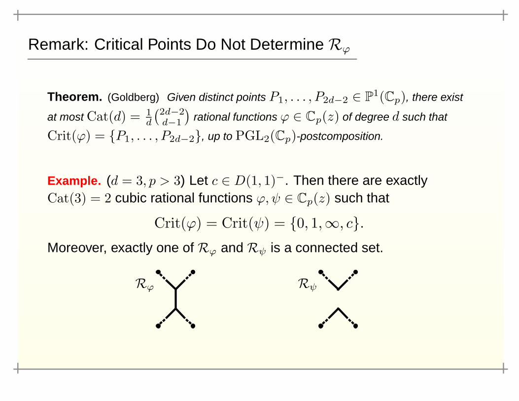
Theorem. (Goldberg) Given distinct points P1, . . . , P2d−2 ∈ P1(Cp), there exist

at most Cat(d) = 1d

(2d−2d−1

)rational functions ϕ ∈ Cp(z) of degree d such that

Crit(ϕ) = {P1, . . . , P2d−2}, up to PGL2(Cp)-postcomposition.

Example. (d = 3, p > 3) Let c ∈ D(1, 1)−. Then there are exactlyCat(3) = 2 cubic rational functions ϕ, ψ ∈ Cp(z) such that

Crit(ϕ) = Crit(ψ) = {0, 1,∞, c}.Moreover, exactly one of Rϕ and Rψ is a connected set.

Rϕ Rψ

Structure of Rϕ

Theorem. (Favre / Rivera-Letelier) The multiplicity mϕ is upper semicontinuous.

If deg(ϕ) > 1, thenRϕ is a nonempty perfect subset of P1.

Theorem. (XF) If ϕ is defined over Cp, then

Rϕ has at most deg(ϕ)− 1 connected components.

Proof Idea: Let X be a connected component of Rϕ, x ∈ X .=⇒ At least 2mϕ(x)− 2 ≥ 2 critical points in X=⇒ ≤ deg(ϕ)− 1 connected components (Hurwitz formula)

This result is best possible: given integers 1 ≤ n < d, there exists arational function ϕ ∈ Cp(z) such that Rϕ has n connected components.(This is a very special construction though.)

Structure of Rϕ

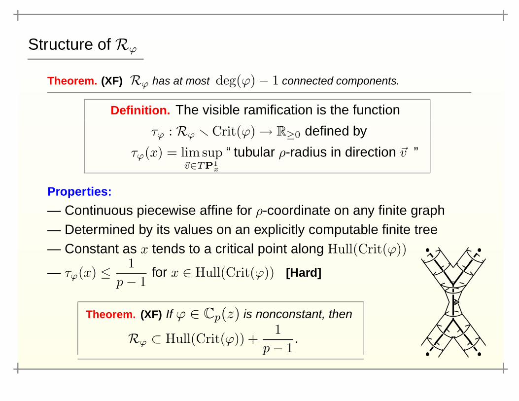
Theorem. (XF) Rϕ has at most deg(ϕ)− 1 connected components.

Definition. The visible ramification is the function

τϕ : Rϕ � Crit(ϕ)→ R≥0 defined by

τϕ(x) = lim sup�v∈TP1

x

“ tubular ρ-radius in direction �v ”

Properties:

— Continuous piecewise affine for ρ-coordinate on any finite graph— Determined by its values on an explicitly computable finite tree— Constant as x tends to a critical point along Hull(Crit(ϕ))

— τϕ(x) ≤ 1p− 1

for x ∈ Hull(Crit(ϕ)) [Hard]

Theorem. (XF) If ϕ ∈ Cp(z) is nonconstant, then

Rϕ ⊂ Hull(Crit(ϕ)) +1

p− 1.

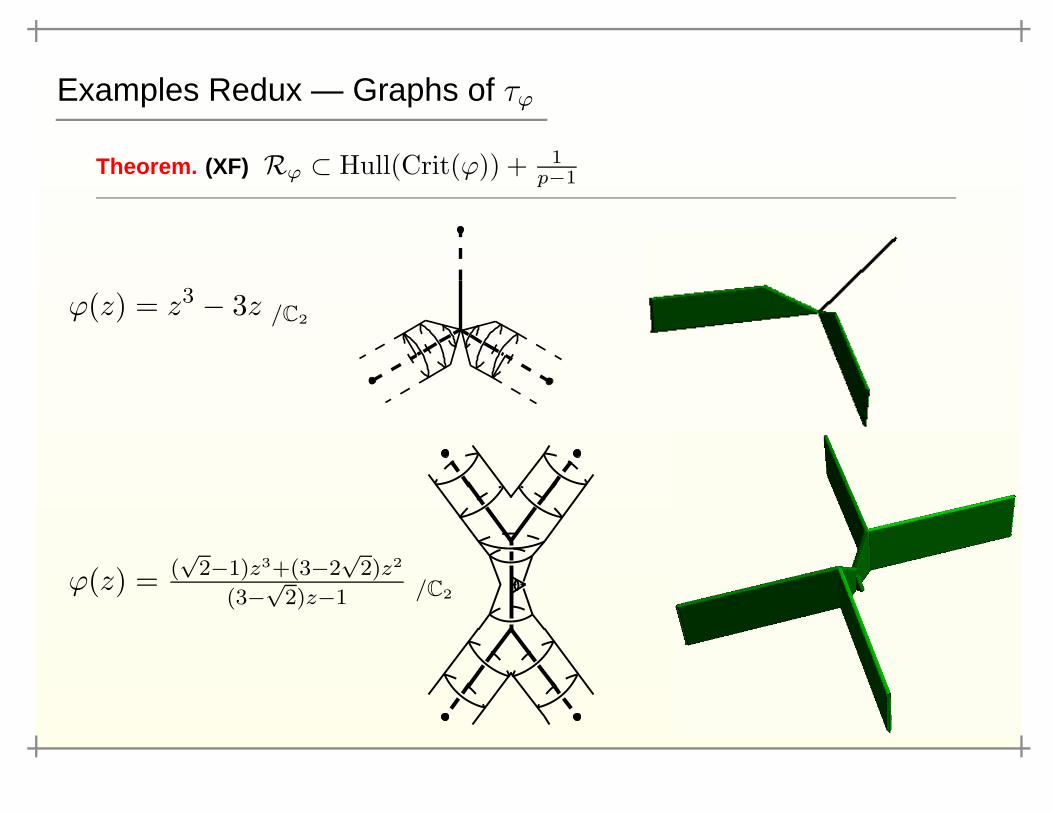
Examples Redux — Graphs of τϕ

Theorem. (XF) Rϕ ⊂ Hull(Crit(ϕ)) + 1p−1

ϕ(z) = z3 − 3z /C2

ϕ(z) = (√

2−1)z3+(3−2√

2)z2

(3−√2)z−1 /C2

A Dynamical Application — with M. Manes and B. Viray

Question: Given ϕ, ψ ∈ Q(z), are they conjugate over Q?

For a field k, write Conjϕ,ψ(k) = {s ∈ Aut(P1k) : s ◦ ϕ ◦ s−1 = ψ}.

Theorem. Fix p > 3 a prime of good reduction for ϕ and ψ. The reduction

map red : Conjϕ,ψ(Q)→ Conjϕ,ψ(Fp) is well-defined and injective.

Corollary. Conjϕ,ψ(Fp) = ∅ for p� 1 =⇒ ϕ is not conjugate to ψ.

Sketch: ϕ has good reduction ⇐⇒ ϕ−1(ζ0,1) = ζ0,1.s ∈ Conjϕ,ψ(Cp) =⇒ s−1(ζ0,1) is totally ramified and fixed for ϕ.=⇒ s−1(ζ0,1) = ζ0,1 by ramification study =⇒ s has good reduction.

red(s) = red(t) ⇒ st−1 ∈ Autϕ(Cp) has trivial reduction⇒ order | p.p = 2 or 3 by classification of finite subgroups of PGL2(Q).

Application: Rolle’s Theorem for Rational Functions

Theorem. (XF) ϕ ∈ Cp(z) nonconstant. If ϕ has at least two

distinct zeros in D(a, r), then it has a critical point in D(a, rp1/(p−1)

).

Classical (due to A. Robert) unless ϕ (D(a, r)) = P1(Cp)

Idea: ≥ 2 zeros ⇒ D(a, r) ∩Rϕ �= ∅

=⇒ D(a, rp1/(p−1)

) ∩ Hull(Crit(ϕ)) �= ∅

Corollary. (XF) ϕ ∈ Cp(z) nonconstant. If ϕ (D(a, r)) = P1(Cp),

then there is a critical point in D(a, rp1/(p−1)

).

Question: Can the latter be refined to D(a, rp1/(p+1)

)?

Final Thoughts

Question: Extend to higher genus curves? (Baldassarri)— Uses p-adic differential equations— case P1 → P1 is the most delicate

Project: Implement an algorithm for computing Rϕ— τϕ is effectively computable

The Future: Rϕ ��������appears to be isometric to a union of ramification loci

of lower degree functions. Could this give a “decomposition” of ϕ intolower degree maps?

ϕ(z) =5z3 − 9z2

3z + 1 /C2

ψ(z) = z2

η(z) =5z − 4

(z − 1)2 0

∞

1

− 35

Rϕ = Rψ ∪Rη