The Black-Litterman Model Towards its use in practice

Charlotta Mankert

Doctoral Thesis in Industrial Economics and Management

Stockholm, Sweden 2010

© Charlotta Mankert The Royal Institute of Technology, KTH Department of Industrial Economics and Management SE 100 44 Stockholm, Sweden Printed by Universitetsservice US AB TRITA-IEO-R 2010:10 ISSN 1100-7982 ISRN/KTH/IEO-R-10:10-SE ISBN 978-91-7415-813-7

Abstract The Black-Litterman model is analyzed in three steps seeking to in-vestigate, develop and test the B-L model in an applied perspective. The first step mathematically derives the Black-Litterman model from a sampling theory approach generating a new interpretation of the model and an interpretable formula for the parameter weight-on-views. The second step draws upon behavioural finance and partly explains why managers find B-L portfolios intuitively accurate and also comments on the risk that overconfident managers state too low levels-of-unconfidence. The third step, a case study, concerns the implementation of the B-L model at a bank. It generates insights about the key-features of the model and their interrelations, the im-portance of understanding the model when using it, alternative use of the model, differences between the model and reality and the influ-ence of social and organisational context on the use of the model. The research implies that it is not the B-L model alone but the com-bination model-user-situation that may prove rewarding.

Overall, the research indicates the great distance between theory and practice and the importance of understanding the B-L model to be able to keep a critical attitude to the model and its output. The re-search points towards the need for more research concerning the use of the B-L model taking cultural, social and organizational contexts into account.

Acknowledgements I would like to take this opportunity to thank some of the people involved in making the work on the thesis possible and enjoyable. First and foremost, I must express my deepest gratitude to Professor Birger Ljung and Associate Professor Harald Lang. Working with you has been a privilege. Our discussions ranging from economics and mathematics to more philosophical issues are always inspiring and very instructive.

Birger, I have been fortunate to have had you as principal supervisor. It was you who first got me thinking about a PhD. During these years you have always patiently, read my texts of varying quality. No matter how preliminary you have never been judgemental and always given constructive feedback on everything from small details to high-level thinking. I will forever be grateful for the dedication and extraordi-nary guidance. Our discussions have not only concerned research, they have involved teaching, work, and life in general - you are an inspiring role model and mentor.

Harald, your rare combination of knowledge of advanced mathemat-ics and insight into the philosophy of economics has been invaluable in the development of this thesis. Thank you for feedback, support and great supervision!

Many thanks to Cefin for financing this research and for generous and interested cooperation. Thank you Professor Kent Eriksson for supporting my research.

Thank you Associate Professor Lars Silver for reading and giving constructive feedback on a late draft of the text. Your contributions have had significant impact on the thesis.

Professor emeritus Claes Gustafsson included me in his group of doctoral researchers. This has been an important and instructive fac-tor in my research education, thank you.

Anders Peterson, thanks for the great collaboration and for nice lunches. “Pete”, “John”, “Bill” and “Eric”, thank you for your co-operation and for reading and commenting a draft of this thesis.

My original Indek crew: Sven Bergvall, Helena Csarman, Mikolaj Dymek, Thomas Lennerfors and David Sköld; We had a lot of fun with everything from small coffee breaks to trips to places such as Reykjavik, Gattieres and Saint Petersburg. I already miss the ryssrullar with loads and loads of trans fats! Stefan Görling, Alexander Löfgren and Lucia Crevani came along as time went by with both more coffee break goodies and great personalities. Thanks all of you for filling my doctoral years with what seemed to be endless fun and laughter.

Others who have contributed to making my doctoral years stimulat-ing and enjoyable include: Fredrik Barchéus, Ester Barinaga, Henrik Blomgren, Albert Danielsson, Marianne Ekman, Kristina Enflo, Mats Engwall, Bertil Guve, Bo Göranzon, Anette Hallin, Maria Ham-marén, Thorolf Hedborg, Matti Kaulio, Ann-Charlotte Kjellberg, Håkan Kullvén, Staffan Laestadius, Marcus Lindahl, Monica Lind-gren, Christer Lindholm, Vicky Long, Lena Mårtensson, Cali Nuur, Johann Packendorff, Kristina Palm, Caroline Pettersson, Erik Piñeiro, Alf Rehn, Jonas Råsbrant, David Sonnek, Tomas Sörensson, Kent Thorén, Pernilla Ulfengren and Thomas Westin.

I would like to thank my family for always supporting me and believ-ing in me and my activities. My little darlings Isidor and Minna, I love you so much! Finally, I want to express my deepest gratitude to my love and “team mate” Daniel Ljungström for his unfailing support on my doctoral journey. What would I have done without you?

Vasastan, 11th November 2010

Charlotta Mankert

TABLE OF CONTENTS 1 Introduction 11 1.1 Aim and Purpose 12 1.2 Rationale 12 1.3 Points of Departure 15 1.4 The Steps 18

Step I: The Sampling Theory Approach to the B-L Model 21

2 Markowitz’ Model 23 2.1 Problems in the Use of Markowitz’ Model 24 2.2 Historical Data 27

3 The B-L Model 29 3.1 The Framework and the Idea 29 3.2 The Bayesian Approach to the B-L Model 36

4 The Sampling Theory Approach to the B-L Model 39

4.1 Derivation 40 4.2 Results 49

Step II: Behavioural Finance and the B-L Model 53

5 Behavioural Finance 55 5.1 The History of Behavioural Finance 56 5.2 The Parts of Behavioural Finance 57 5.3 Behavioural Finance and Quantitative

Financial Models 59

6 Behavioural Finance and the B-L Model 62 6.1 The B-L Model and the Utility Function 63 6.2 The B-L Model and Overconfidence 72 6.3 Behavioural Finance and the B-L Model –

What it gave and didn’t give? 83

Step III: The B-L Model in Practice 87

7 Introducing Step III 89 7.1 Input from Step I and II 89 7.2 Academic Positioning 90 7.3 Outlining Step III 93

8 The Case 94 8.1 Start Up 94 8.2 The WM group at SIB Private Banking 95 8.3 Implementing 100 8.4 Case Crisis 101 8.5 Testing 102

9 Method 104 9.1 Case Study Research 105 9.2 Action Science 106 9.3 Empirical Material 110 9.4 Trustworthiness 112 9.5 Writing 113

10 The B-L Features 115 10.1 Views 116 10.2 Levels-of-unconfidence 125 10.3 Weight-on-views 132 10.4 Conclusions: The B-L Features 134

11 Model Issues Unlooked-for 135 11.1 Several Benchmark Portfolios 135 11.2 Assets not included in SIBLImp 140 11.3 Fund or Asset Class Level 141 11.4 Conclusions: Model Issues Unlooked-for 145

12 The B-L Model in Allocation 147 12.1 The August 2008 Allocation 148 12.2 The September 2008 Allocation 155 12.3 Reflections on the Experiences from

Using SIBLImp 157 12.4 Conclusions: The B-L Model in Allocation 160

13 Organizational Issues 162 13.1 The WM group and SIB PB 162 13.2 Project Issues 165 13.3 Importance of Enthusiasts 168 13.4 Conclusions: Organisational Issues 168

14 Results and Comments on the Case 169 14.1 Results 169 14.2 Comments on the Case 174 14.3 Case Epilogue 175

Ending 179

15 Concluding Discussion 181 15.1 Summary of Results 181 15.2 Strong Impressions 183 15.3 Moving On… 185

Literature 189 Appendix 1 201 Appendix 2 203 Appendix 3 205 Appendix 4 218 Appendix 5 221 Appendix 6 223

11

1 Introduction In 1952 Markowitz published his article Portfolio Selection, which can be seen as the genesis of modern portfolio theory. Portfolio models are intended to help portfolio managers decide the weights of the assets within a fund or a portfolio. Markowitz’ ideas have had a great impact on portfolio theory and have, theoretically, withstood the test of time. However, in practical portfolio management Markowitz’ model has not had the same impact as in academia. Fund and portfolio manag-ers consider the composition of portfolios generated by the Markow-itz model to be unintuitive (Michaud, 1989; Black & Litterman, 1992).

The practical problems in using the Markowitz model motivated Fisher Black and Robert Litterman to develop a new model in the early 1990s. The model, often referred to as the Black-Litterman model (hereafter the B-L model), builds on Markowitz’ model and aims at handling some of its practical problems. The B-L model uses what Black and Litterman refer to as the equilibrium portfolio, often assessed as the benchmark weights of the assets in a portfolio, as a point of reference. “Bets” or deviations from the equilibrium port-folio are taken on assets to which the portfolio managers have as-signed views. To each view, the manager assigns a level-of-

12

unconfidence1, indicating how sure he/she is of that particular view. The views and levels-of-unconfidence affect how much the output portfolio differs from the equilibrium portfolio.

This thesis reports the results from three studies seeking to investi-gate, develop and test the B-L model in an applied perspective.

1.1 Aim and Purpose The overall aim of the thesis is to contribute to the develop-ment of the B-L model viewed as a tool for portfolio manage-ment.

The thesis consists of three steps. Each step has its own, more spe-cific aim and purpose, but they are closely connected and all point in the same direction, toward research contributing to the development of the B-L model.

The aim of the first step is to develop the B-L model and to fill knowledge gaps especially concerning the parameter “weight-on-views” by providing a careful description of the mathemati-cal derivation of the model from a sampling theoretical ap-proach.

The aim of the second step is to draw implications from re-search results within behavioural finance that are relevant to the B-L model.

The aim of the third step is to examine the development and use of an implementation of the B-L model at a Swedish bank; to discuss and draw conclusions from these experiences that can contribute to the development of the B-L model.

1.2 Rationale The thesis should be viewed in the light of the fact that qualitative, empirical research is scarce in financial research in general and no such study of the B-L model seems to exist. Also, new financial re-search streams (further discussed in chapter 7.2) express the need to expand financial knowledge with research involving those actually

1 This variable is often referred to as levels of confidence. In this thesis levels-of-unconfidence will instead be used.

13

acting in the field being studied. Mackenzie (2005b) claims that the only way of opening the “black boxes” of financial markets is to interact with those involved in constructing the box. In this case the B-L model could be seen as the black box and to be able to learn about and develop the B-L model we therefore need to interact with those using it. Hence, this also points in the direction of qualitative case study research.

The knowledge, academic and non-academic, relating to the model, however, appeared to be somewhat insufficient. The existence of articles with names such as: “The demystification of the Black-Litterman model” (Satchell & Scowcroft, 2000), “The intuition be-hind the Black-Litterman model portfolios” (He & Litterman, 1999) and “A step-by-step guide to the Black-Litterman model” (Idzorek, 2004) indicated that difficulties existed within the model. To be able to perform a case study on the use of the model a deep understand-ing of the model seemed to be a prerequisite. However, when trying to obtain such understanding, theoretical shortcomings in the model were revealed. Some parameters were not properly described and the model was surrounded with a great deal of vagueness. One of the most severe problems in the model was related to the parameter of-ten referred to as the weight-on-views or tau. Reasoning concerning this parameter was quite weak in existing literature. While Black and Litterman (1992, p. 17) suggest that weight-on-views should be close to zero, Satchell and Scowcroft (2000) argue that they are often set to 1. Bevan and Winkelmann (1998, p. 4), propose that weight-on-views can be set so that the information ratio2 does not exceed 2.0 and have found that it, in practice, often lies between 0.5-0.7. He and Litter-man (1999, p. 6) claim that weight-on-views need not be set at all. Hence, there were totally different suggestions as to what value the parameter ought to be set and discussions concerning these values were quite limited.

Since understanding is essential when it comes to using quantitative financial models, it seemed unreasonable to do empirical research

2 A risk measure of how well a fund is paid for the active risk taken, hence how much extra the fund returns by deviating from the index portfolio.

14

before a deeper understanding of the model had been obtained. As a consequence, a theoretical study was carried out. In the first step of the research the B-L model is therefore mathematically derived from a sampling theory approach. This step solves the problems of theo-retical knowledge gaps within the model and generates an interpre-table formula for weight-on-views. With deeper knowledge about the B-L model, the plan was then to do case study research concerning the use of the model.

However, behavioural finance discusses the behaviour of individuals when making judgment under uncertainty, an important part of port-folio management and the use of the B-L model. To be well equipped with knowledge concerning the behaviour of individuals in financial decision-making and thereby sharpening the case study research con-cerning the B-L model, it seemed reasonable to study behavioural finance and to draw implications from research results from the field to the use of the B-L model.

When that was done, it was time to carry out the empirical research. The third step of the thesis concerns empirical action research per-formed at a large Swedish investment bank where they had used a B-L inspired program in their portfolio management process for a year, but now wanted help to continue this work. The case mainly con-cerns the implementation and development process of a new B-L tool at the bank, but also takes up the program they worked with before as well as a program implemented in the work of getting ac-cess to this case.

My personal interest in the B-L model derives from a project in 2002, more thoroughly discussed in appendix 1. The project indicated that actors within the financial industry were interested in the B-L model, which was also corroborated by interviews with portfolio managers, in 2006. Six out of seven of these portfolio managers claimed to rec-ognize the B-L model, three expressed a genuine interest in the model, one had quite detailed knowledge about the model and one used a B-L inspired tool in the allocation process.

15

1.3 Points of Departure The overall research has been guided by the following basic points of departure.

A model The B-L model is a model. In the essence of models lies that they differ from reality; they are simplifications. Wiener (1945) makes a nice comment when he claims that “The best material model of a cat is another cat, or preferably, the same cat”. However, the model still needs to be a good representation of the important properties of the reality it is supposed to mirror. Derman and Wilmott (2009) appreciate sim-plicity in financial models, but assert that it is the models that are simple and not reality. They claim:

The most important question about any financial model is how wrong it is likely to be, and how useful it is despite its assump-tions.

(Derman & Wilmott, 2009, p. 2)

Much of financial modelling is inspired by physics. There are, how-ever, fundamental differences between these fields. While physics models relatively stable systems and material objects, financial models are much more fragile systems that are constructed by human beings. Human behaviour is much more diverse and often more difficult to model than material objects. Despite the differences, financial theory has largely sought to develop theories as stable and with the same ability to forecast as physics has done. Derman and Wilmot (2009) state that there are no fundamental laws of finance as there are in physics. If there were, it would nevertheless be impossible to, as in physics, make repeated experiments to verify them.

Understanding The fact that financial modelling involves simplifications and that implementing such models involves estimations of different kinds suggests the need for users to understand the models they work with. It is hence essential that users of the B-L model do understand the theoretical characteristics and limits of the model as well as the spe-cific implementation with which they are working. This obviously also applies to researchers who study and develop the B-L model.

16

By understanding the model and the specific implementation it might be possible to maintain a critical attitude towards the output of the model and its use. Understanding provides a possibility to see that the model is wrong, the implementation is bad, the estimations are not good under these market circumstances, the input is wrongly ex-pressed or the input is wrong in itself and so on. Derman (2004, p. 269) writes about financial models: “Models are better regarded as a collec-tion of parallel thought universes you can explore”. To be able to explore these universes understanding them is essential. Hence, one point of departure in this thesis is that understanding the B-L model and the implementation of the same is important for researching as well as using the model.

A tool The B-L model is regarded as a tool to be used in a social and organi-zational context. The model is seen as having the possibility of being a useful tool and thereby assisting portfolio managers or investors in investment decisions. The value of a tool used in an investment con-text is not only dependent on its theoretical characteristics. The most theoretically advanced and elegant model might actually be impos-sible to use. For a tool to be valuable, a tool needs to work well in practice.

A process The B-L model is not perceived as a finished model that needs to be demystified, but as an idea that has been and is being developed over time, hence the development is an on-going process. The article Glo-bal Portfolio Optimization by Black and Litterman (1992) is an initial and central contribution to the process of developing the B-L model. When referring to the B-L model it is not only the model as explained by Black and Litterman that is considered, but also everyone working with the B-L model, including myself, are contributors to and partici-pants in the development process.

This thesis aims to contribute to the process of developing the B-L model. It consists of three steps. Although these are of quite different character and draw upon different research traditions and fields, there exists both a clear connection and a progression between them. The three steps are also based on each other. Hence, the first step lays the

17

foundation for the second. When moving from the first step, where the B-L model is mathematically derived, the model has changed; a step has been taken in the development process. The model is in a way rebuilt: some variables have new formulas and the model is in-terpreted and derived in another way. Performing empirical research in practical portfolio management (step III) builds on the knowledge and experience from the two first steps. Steps one and two indicate the need for practical empirical research concerning the use of the model. The theories, both portfolio theory and behavioural finance, are individualistic in character and with little reference to social and organizational contexts. Hence, step three is intended to generate new knowledge concerning the use of the B-L model. The process will continue after this thesis is concluded.

Broad perspective The research project has a broad perspective. It aspires to go “all the way” from the theoretical characteristics of the model to its practical use in organizations. This requires interaction with different research traditions and cultures. The project may therefore be seen as a cross-disciplinary project or perhaps rather an interdisciplinary project (Vetenskapsrådet, 2005). Cross-disciplinary or interdisciplinary re-search can be difficult, demanding both methodological and theoreti-cal knowledge from different research fields. One strategy for han-dling the interdisciplinary approach has been to have supervision from two different academic cultures: one of the supervisors of the research has a more mathematical focus, working in the Mathematics department while my main supervisor holds a more organizational perspective, working in the Industrial Management and Organization department. Also, a conscious choice was made to join different kinds of seminars and other activities to gain insight into different academic cultures and thereby attain broadened perspectives on what research is about. Keeping up with a group of researchers with a qualitative research approach has been very instructive. Reading about and discussing issues like social constructivism, post modern-ism, critical theory, grounded theory and so on have influenced the research performed and the attitude towards what should be studied, why and how. The arrangement has, as I see it, been helpful in the research process. Performing research under these circumstances has influenced the work in many ways. Working with researchers in the

18

Department of Industrial Management and Organization with a more qualitative and organizational approach hopefully helped me maintain a distanced and critical attitude towards research results within the different financial fields. This distance has been a prerequisite for taking step two and three.

1.4 The Steps Below follows a brief presentation of the three steps that constitute the thesis.

Step I: The sampling theory approach to the B-L model The mathematical derivation of the B-L model serves as a prerequi-site for doing case study research on the use of the model. Motives for step I are:

• The literature concerning theoretical characteristics of the B-L model is insufficient.

• Mathematical explanations of some of the variables within the model are absent and therefore cannot be interpreted by either researchers or users.

• Fruitful research and use of quantitative financial models re-quires researchers and users to be familiar with the theoretical foundations of the model.

The B-L model is derived using a sampling theory approach. Existing literature concerning the B-L model takes a Bayesian approach. Al-though suggested by Black and Litterman (1992) the sampling theory approach does not appear in literature. A derivation using this ap-proach will hopefully provide a way for people unfamiliar with Bay-esian theory to understand the theoretical characteristics of the model.

Step II: Behavioural finance and the B-L model Using the B-L model demands actions: judgments and estimations. Since much research within behavioural finance concerns the behav-iour of individuals in investment situations, step II searches the field for research relevant to the use of the B-L model. The aim is not to

19

find all research that might have some kind of implications for the use of the B-L model. Instead the focus is on:

• Research results relevant to features specific to the B-L model.

• Results that are robust and well established.

To find such research, a literature review has been prepared, pre-sented in appendix 3. This does not aspire to be exhaustive.

Step III: The B-L model in practice The third step is a case study performed at a large investment bank. It builds on action science and concerns the development of a program implementing the B-L model. It presents and discusses experiences from the project focusing on the main features of the B-L model as well as other more unexpected problems and organizational concerns. The study called for a position to be taken on a variety of method-ological issues. These are discussed separately in chapter 9.

21

STEP I

The Sampling Theory Approach to the B-L Model The aim of the first step of this thesis is to develop the B-L model and to fill knowledge gaps, especially concerning the parameter “weight-on-views”, by providing a careful description of the math-ematical derivation of the model from a sampling theory approach.

The B-L model builds on Markowitz’ classical portfolio model and aims at handling some of the problems in its practical use. The first step of this study begins with a brief presentation of Markowitz’ model and a discussion concerning problems connected to its use. After the presentation of Markowitz’ model a thorough description of the concept and the framework behind the B-L model is pre-sented. A brief presentation of the Bayesian approach – the more commonly used approach to the B-L model – follows before the sampling theory approach to the B-L model is presented and derived. Although suggested by Black and Litterman (1992), this approach does not seem to appear in the literature. Step I is then concluded with a summary and discussion of the results. But let us start with Markowitz’ model, the model that the B-L model aims to improve.

23

2 Markowitz’ Model Portfolio theory took form as an academic field when Harry Markow-itz published the article Portfolio Selection in 1952. Markowitz focuses on a portfolio as a whole; instead of security selection he discusses portfolio selection. Previously, little research concerning the math-ematical relations within portfolios of assets had been carried out. Markowitz began from John Burr Williams’ Theory of Investment Value. Williams (1938) claimed that the value of a security should be the same as the net present value of future dividends. Since the future dividends of most securities are unknown, Markowitz claimed that the value of a security should be the net present value of expected fu-ture returns. Markowitz claims that it is not enough to consider the characteristics of individual assets when forming a portfolio of finan-cial securities. Investors should take into account the co-movements represented by covariances of assets. If investors take covariances into consideration when forming portfolios, Markowitz argues that they can construct portfolios that generate higher expected return at the same level of risk or lower level of risk with the same level of expected return than portfolios ignoring the co-movements of asset returns. Risk, in Markowitz’ model (as well as in many other quantita-tive financial models) is assessed as the variance of the portfolio. The variance of a portfolio in turn depends on the variance of the assets in the portfolio and on the covariances between its assets.

24

Markowitz’ mean-variance portfolio model is the base on which much research within portfolio theory is performed. It is also from this model that the B-L model was developed. The B-L model builds on the Markowitz model. A summary of the model is provided in this chapter, with focus on the practical problems encountered in the use of the model. The practical problems in using Markowitz’ model prompted Black and Litterman to continue the development of port-folio modelling.

Markowitz shows that investors under certain assumptions, theoreti-cally, can build portfolios that maximize expected return given a speci-fied level of risk, or minimize the risk given a level of expected re-turn. The model is primarily a normative model. The objective for Markowitz has been not to explain how people select portfolios, but how they should select portfolios (Sharpe, 1967). Even before 1952 diversification was a well-accepted strategy to lower the risk of a port-folio, without lowering the expected return, but until then, no thor-ough foundation existed to validate diversification. Markowitz’ mean-variance portfolio model has remained to date the cornerstone of modern portfolio theory (Elton & Gruber, 1997).

2.1 Problems in the Use of Markowitz’ Model

Although Markowitz’ mean-variance model might seem appealing and reasonable from a theoretical point of view, several problems arise when using the model in practice. In the article The Markowitz optimization Enigma: Is “Optimized” Optimal? (1989), Michaud thor-oughly discusses the practical problems of using the model. He claims that the model often leads to irrelevant optimal portfolios and that some studies have shown that even equal weighting can be superior to Markowitz optimal portfolios. Michaud argues that the most im-portant reason for many financial actors not to use Markowitz’ model is “political”. The fact that the quantitatively oriented specialists would have a central role in the investment process would intimidate more qualitatively oriented managers and top level managers, accord-ing to Michaud. The article was however written 15 years ago and this may no longer be the most important reason for not using Markow-

25

itz’ model. In the article Michaud also reviews other disadvantages of using the model.

The most important problems in using Markowtiz’ model are:

1. According to Michaud (1989) and Black and Litterman (1992), Markowitz’ optimizers maximize errors. Since there are no cor-rect and exact estimates of either expected returns or variances and covariances, these estimates are subject to estimation errors. Markowitz’ optimizers overweight securities with high expected return and negative correlation and underweight those with low expected returns and positive correlation. These securities are, according to Michaud, those that are most prone to be subject to large estimation errors. The argument appears however some-what contradictory. The reason for investors to estimate high ex-pected return on assets should be that they believe that this asset is prone to return well. It then seems reasonable that the manager would appreciate that the model overweighs this asset in the portfolio (taking covariances into consideration).

2. Michaud claims that the habit of using historical data to produce a sample mean and replace the expected return with the sample mean is not a good one. He claims that this line of action contri-butes greatly to the error-maximization of the Markowitz mean-variance model.

3. Markowitz’ model doesn’t account for assets’ market capitaliza-tion weights. This means that if assets with a low level of capitali-zation have high-expected returns and are negatively correlated with other assets in the portfolio, the model can suggest a high portfolio weight. This is actually a problem, especially when add-ing a shorting constraint. The model then often suggests very high weights in assets with low level of capitalization.

4. The Markowitz mean-variance model does not differentiate be-tween different levels of uncertainty associated with the estimates input to the model.

5. Mean-variance models are often unstable, meaning that small changes in input might dramatically change the portfolio. The

26

model is especially unstable in relation to the expected return in-put. One small change in expected return on one asset might generate a radically different portfolio. According to Michaud this mainly depends on an ill-conditioned covariance matrix. He exemplifies ill-conditioned covariance matrixes by those esti-mated with “insufficient historical data”.

Michaud also discusses further problems with Markowitz mean-variance model. These are: non-uniqueness, exact vs. approximate mean-variance optimizers, inadequate approximation power and de-fault settings of parameters.

One of the most striking empirical problems, in using the Markowitz model, is that when running the optimizer without constraints, the model almost always recommends portfolios with large negative weights in several assets (Black & Litterman, 1992). Fund or portfolio managers using the model are often not permitted to take short posi-tions. Because of this, a shorting constraint is often added to the optimization process. What happens then is that when optimizing a portfolio with constraints, the model gives a solution with zero weights in many of the assets and therefore takes large positions in only a few of the assets and unreasonable large weights in some as-sets. Many investors find portfolios of this kind unreasonable and although it seems, as though many investors are appealed to the idea of mean-variance optimization, these problems appear to be among the main reasons for not using it. In a world in which investors are quite sure about the input to an optimization model, he output of the model would not seem so unreasonable. In reality however, every approximation about future return and risk is quite uncertain and the chance that it is “absolutely correct” is low. Since the estimation of future risk and return is uncertain, it seems reasonable that investors wish to invest in portfolios which are not prospective disasters if the estimations prove incorrect. Markowitz’ model has been shown, how-ever, to generate portfolios that are very unstable i.e. sensitive to changes in input (Fisher & Statman, 1997), meaning that a small change in input radically changes the structure of the portfolio. Michaud (1989) claims that better input estimates could help bridge problems of the unintuitiveness of Markowitz’ portfolios. Fisher and Statman, however, maintain that although good estimates are better

27

then bad, better estimates will not bridge the gap between mean-variance optimized portfolios and “intuitive” portfolios, in which investors are willing to invest, since estimation errors can never be eliminated. It is not possible to predict future expected returns, vari-ances and covariances with 100% confidence.

Estimating covariances between assets is also problematic. In a port-folio containing 50 assets the number of variances that need to be estimated is 50, but the number of covariances that need to be esti-mated is 1225. This seems to be much for a single portfolio manager to handle. It also seems much for an investment team, consisting of several persons. According to Markowitz (1991, p. 102) “in portfolios involving large numbers of correlated securities, variances shrink in importance compared to covariances”.

Although there exist several quite severe disadvantages in the use of the Markowitz mean-variance model, the idea of maximizing ex-pected return; minimizing risk or optimizing the trade-off between risk and expected return is so appealing that the search for better-behaved models has continued. The B-L model is one of these and the model has gained much interest in recent years.

2.2 Historical Data There seems to exist a common misconception saying that Markow-itz’ theories and model build solely on historical data. This, however, is not the case. Markowitz asserts that various types of information can be used as input to a portfolio analysis:

One source of information is the past performance of individ-ual securities. A second source of information is the beliefs of one or more security analysts concerning future performances.

(Markowitz, 1991, p. 3)

Portfolio selection should be based on reasonable beliefs about future returns rather than past performances per se. Choices based on past performances alone assume, in effect, that aver-age returns of the past are good estimates of the ‘likely’ return in the future; and variability of return in the past is a good measure of the uncertainty of return in the future.

(Markowitz, 1991, p. 14)

28

Markowitz (1991) is quite clear that he focuses on portfolio analysis and not security analysis. He claims that he does not discuss how to arrive at a reasonable belief about securities since this is the job of a security analyst. Markowitz’ contribution begins where the contribu-tion of the security analysis leaves off. While Markowitz time and time again repeats that historical data alone is inadequate as a basis for estimating future returns and covariances, we can often read about the importance of historical data in modern financial theory. It is hard to question the fact that historical time series have had great impact on financial decision-makings.

…covariance matrices determined from empirical financial time series appear to contain such a high amount of noise that their structure can essentially be regarded as random. This seems, however, to be in contradiction with the fundamental role played by covariance matrices in finance, which constitute the pillars of modern investment theory and have also gained in-dustry-wide applications in risk management.

(Pafka & Kondor, 2002, Abstract)

There seems to be a general confusion between the covariances of future returns and covariances estimated from historical data. This is problematic and may affect the discussion and the development of portfolio theory. The discussion whether historical data is a good approximation for future covariance matrices is, to me, interesting and also important. Also, I believe that it is of importance to discuss whether it is possible at all to make reasonable estimates of future covariances and how this affects the use of portfolio modelling. Sepa-rating the two discussions would however probably be productive.

29

3 The B-L Model The problems encountered when using Markowitz’ model in practical portfolio management and the fact that mean-variance optimization hasn’t had such a high impact in practice motivated Fisher Black and Robert Litterman to work on the development of models for port-folio choice. Black and Litterman (1992) proposed a means of esti-mating expected returns to achieve better-behaved portfolio models. However they require the portfolio to be at the efficient frontier. If this is not the case, it may be possible to obtain a “better” portfolio from a mean-variance perspective. The B-L model is often referred to as a completely new portfolio model. Actually the B-L model differs only from the Markowitz model with respect to the expected returns. The B-L model is otherwise theoretically quite similar to Markowitz’ mean-variance model. How the B-L expected returns are to be esti-mated has been found to be quite complicated. The model generates portfolios differing considerably from portfolios generated by using Markowitz’ model.

3.1 The Framework and the Idea The B-L model was developed to make portfolio modelling more useful in practical investment situations (Litterman, 2003c, p. 76). To do this, Black and Litterman (1992) apply, what they call, an equilib-

30

rium approach. They set the idealized market equilibrium as a point of reference. The investor then specifies a chosen number of market views in the form of expected returns and a level-or-unconfidence for each view. The views are combined with the equilibrium returns and the combination of these constitutes the B-L expected returns. The B-L expected returns are then optimized in a mean-variance way, creating a portfolio where bets are taken on assets where investors have opinions about future expected returns but not elsewhere. The size of the bets, in relation to the equilibrium portfolio weights, de-pends on the confidence levels specified by the user and also on a parameter specifying the weight of the collected investor views in relation to the market equilibrium, the weight-on-views.

The following notation is used:

€

w * - The weight vector of the B-L unconstrained optimal port-folio.

€

wM - The weight vector of the market capitalized portfolio, re-

ferred to as the equilibrium portfolio or the market portfolio.

€

δ - The risk aversion factor. It is according to Black and Litter-man (1991, p. 37) proportionality constant based on the for-

mulas in Black (1989).

€

δ =µP

σ P2

(Satchell & Scowcroft 2000, p.

139). In He and Litterman (1999) use “

€

δ = 2.5 as the risk aver-sion parameter representing the world average risk tolerance”.

€

Σ - The covariance matrix containing variances of and covarian-ces between all the assets handled by the model.

€

P - A matrix representing the view-portfolios. Each row in the ma-trix contains the weights of assets of one view, i.e. one view portfolio. The maximum number of rows, i.e. the maximum number of views equals the number of assets in the port-folio.

€

q - A column vector that represents the estimated expected re-turns in each view, view-expected-returns.

31

€

ω i - The level-of-unconfidence3 assigned to view i. It is the standard deviation around the expected return of the view so that the investor is 2/3 sure that the return will lie within the interval.

€

Ω - A diagonal matrix consisting of

€

ω1

2,…,ωk

2 .

€

τ - A parameter often referred to as the weight-on-views.

€

τ is a constant, which together with

€

Ω determines the weighting between the view portfolio and the equilibrium portfolio.

€

µ * - This is the B-L modified vector of estimated expected re-turns.

€

Π - The column vector of equilibrium expected excess returns.

To derive the B-L expected returns estimated by the market, the fol-lowing problem is solved:

€

maxΠ

(w M )T Π −δ2

(w M )T ΣwM

equilibrium excess returns,

€

Π is

€

Π = δΣwM (3.1)

This formula represents the expected returns estimated by the mar-ket. Many managers, however, do not wish to invest in the market portfolio. They have views that differ from the market returns. The market returns are then combined with investor views and a modified vector of expected returns constituting the B-L vector of expected returns is created. This new vector of B-L expected returns is then optimized in a mean-variance manner, yielding the formula for the weights of the optimal portfolio. The formula for the Black-Litterman optimal portfolio, without constraints, is presented below. Readers need not understand this formula at this point - a detailed derivation and explanation will be given further on in this chapter.

3 This variable is often referred to as levels of confidence. In this thesis levels-of-unconfidence will instead be used. When the confidence of a view increases the levels of unconfidence de-creases.

32

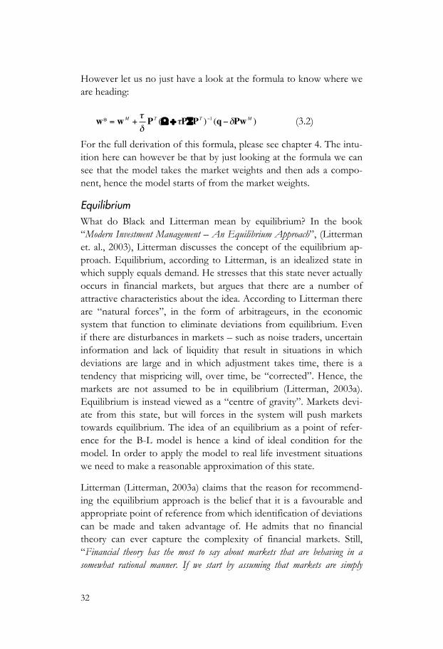
However let us no just have a look at the formula to know where we are heading:

€

w* = wM +

τδ

PT (Ω + τPΣP

T )−1 (q−δPwM ) (3.2)

For the full derivation of this formula, please see chapter 4. The intu-ition here can however be that by just looking at the formula we can see that the model takes the market weights and then ads a compo-nent, hence the model starts of from the market weights.

Equilibrium What do Black and Litterman mean by equilibrium? In the book “Modern Investment Management – An Equilibrium Approach”, (Litterman et. al., 2003), Litterman discusses the concept of the equilibrium ap-proach. Equilibrium, according to Litterman, is an idealized state in which supply equals demand. He stresses that this state never actually occurs in financial markets, but argues that there are a number of attractive characteristics about the idea. According to Litterman there are “natural forces”, in the form of arbitrageurs, in the economic system that function to eliminate deviations from equilibrium. Even if there are disturbances in markets – such as noise traders, uncertain information and lack of liquidity that result in situations in which deviations are large and in which adjustment takes time, there is a tendency that mispricing will, over time, be “corrected”. Hence, the markets are not assumed to be in equilibrium (Litterman, 2003a). Equilibrium is instead viewed as a “centre of gravity”. Markets devi-ate from this state, but will forces in the system will push markets towards equilibrium. The idea of an equilibrium as a point of refer-ence for the B-L model is hence a kind of ideal condition for the model. In order to apply the model to real life investment situations we need to make a reasonable approximation of this state.

Litterman (Litterman, 2003a) claims that the reason for recommend-ing the equilibrium approach is the belief that it is a favourable and appropriate point of reference from which identification of deviations can be made and taken advantage of. He admits that no financial theory can ever capture the complexity of financial markets. Still, “Financial theory has the most to say about markets that are behaving in a somewhat rational manner. If we start by assuming that markets are simply

33

irrational, then we have little more to say” (Litterman, 2003a). He refers to the extensive amount of literature we can access if we are willing to accept the assumption of arbitrage-free markets. According to Lit-terman, we also need to add the assumption that markets, over time, move toward a rational equilibrium in order to take advantage of portfolio theory. He states that portfolio theory makes predictions about how markets will behave, tells investors how to structure their portfolios, how to minimize risk and also how to take maximum advantage of deviations from equilibrium.

Much literature concerning the B-L model assumes a global asset allocation model, and because of this Litterman (2003c) argue that the global Capital Asset Pricing Model (CAPM) is a good starting point for a global equilibrium model. Black (1989) discusses an equi-librium model providing a framework from which the B-L global asset allocation model has emerged. However, the B-L model is not used only in global asset management, but also in domestic equity portfolio management and fixed income portfolio management. In such cases the equilibrium weights are easier to find by using the domestic CAPM.

There is an obvious problem in using equilibrium weights as a point of reference since these weights are not observable and hence must be estimated. Bevan and Winklemann (1998), present a way of deal-ing with this. If the market is in equilibrium, a representative investor will hold a part of the capitalization-weighted portfolio. Many inves-tors are evaluated according to a benchmark portfolio. Often the benchmark is a capitalization-weighted index (Litterman, 2003b). The equilibrium portfolio is then approximated as the benchmark port-folio. These estimated expected returns could be seen as the expected returns estimated by the market if all actors on the market act in a mean-variance manner. Expected equilibrium returns are calculated from the benchmark weights using formula 3.1. As Schachter et al. (1986, p. 254) write: “[T]he price of a stock is more than an objective, ration-ally determined number; it is an opinion, an aggregate opinion, the moment-to-moment resultant of the evaluation of the community of investors.” For each asset, to which the investor has no view, this is what will be handed over to the optimizer. For the assets to which the investor has views, modified expected returns are calculated as a combination of the

34

benchmark weights and the investor views. This way of estimating the equilibrium portfolio is what will be used in this chapter. From now on the equilibrium portfolio often will be referred to as the mar-ket portfolio.

Investor views and levels-of-unconfidence The B-L idea is to combine the equilibrium with investor-specific views. To each view a level-of-unconfidence is to be set by the man-ager. The model allows the investor to express both absolute and relative views. An example of an absolute view is “I expect that equities in country A will return X%” an example of a relative view is “I believe domestic bonds will outperform domestic equities by Y%”. In traditional mean-variance portfolio optimization, relative views cannot be expressed. To each view, whether stated in the relative or absolute form the investor also shall assign a level-of-unconfidence. The level-of-unconfidence is expressed as the standard deviation around the ex-pected return of the view. If managers feel confident in one view the standard deviation should be small and if they are not confident in a view, the standard deviation should be large. The confidence level affects the influence of a particular view. The weaker confidence that is set to a view the less the view affects the portfolio weights. This is considered as an attractive feature since views most often are incor-rect. Views however indicate on which assets investors want to take bets and in which direction the bets ought to be taken.

Combining views with the equilibrium expected returns The B-L optimal portfolio is a weighted combination of the market portfolio and the views of the investor. The views are combined with the equilibrium, and positions are taken in relation to the benchmark portfolio on assets to which investors have expressed views. The size of the bet taken depends on three different variables: the views, the level-or-unconfidence assigned to each view and the weight-on-views. It depends on the views specified by the investor. Views that differs much from the market expected returns contributes to larger bets. If the level-or-unconfidence assigned to a view is strong, this also con-tributes to larger bets. The more confidence the investor assigns to a view, the larger the bets are on that particular asset. The matrix

€

Ω represents the levels-of-unconfidence of the views. There is however one more variable that affects the size of the bets taken in relation to

35

the equilibrium portfolio. The variable

€

τ , the weight-on views (Bevan & Winkelmann, 1998), determines, with

€

Ω , how much weight is to be set on the set of view portfolios specified by the investor in relation to the equilibrium portfolio. I have found no clear description of this variable in existing literature. There seem to be quite different ideas on how to set this variable. Black and Litterman (1992, p. 17) pro-pose that the constant should be set close to zero “because the uncer-tainty in the mean is much smaller than the uncertainty in the return itself”. Satchell and Scowcroft (2000) however claim that

€

τ often is set to 1, but they also claim that this is not always successful in reality. Bevan and Winkelmann (1998, p. 4), on the other hand, suggest that

€

τ can be set so that the information ratio4 does not exceed 2.0. They have found that

€

τ most often lies between 0.5 – 0.7. He and Litterman (1999, p. 6), on the other hand, claim that

€

τ need not be set at all, since only

€

τ −1Ω enters the model. Mathematically, this is correct, but then there would be no point in specifying these two different vari-ables from the beginning. The reasoning concerning

€

τ is hence quite weak in existing literature. The articles don’t express any associations to normative and descriptive argumentation. There are totally differ-ent suggestions on what

€

τ ought to be set to and explanations of why these are reasonable values of

€

τ is not given properly.

By the end of this chapter an interpretable formula to the weight-on-views will however be derived and explained. One of the great advantages of taking a sampling theoretical approach to the B-L model is that it provides an interpretable formula to the weight-on-views. The chapter won’t however result in a recommended value of

€

τ , the formula however will give the user of the B-L model guidance in setting this variable.

When no investor views are specified, the B-L model recommends holding the market portfolio. If investors have no opinion about the market they should not place bets in relation to the equilibrium weights. However, if they have opinions about assets, it seems rea-sonable that the bets are placed in those assets and the rest of the

4 A risk measure, measuring how well a fund is paid for the active risk taken, hence how much extra the fund returns by deviating from the index portfolio.

36

assets have weights close to the market-capitalized portfolio. The stronger confidence assigned, to both the individual view and the weight-on-views, the more the output portfolio deviates from the market portfolio.

Below a brief description of the Bayesian approach to the B-L model is given before the sampling theoretical approach is presented. The sampling theoretical approach will then provide a detailed derivation of the B-L expected returns and the B-L portfolio.

3.2 The Bayesian Approach to the B-L Model Most of the literature concerning the B-L model makes use of a Bay-esian5 approach to construe the B-L model. The approach combines prior information (information considered as relevant although not necessarily in the form of sample data) with sample data. Through repeated use of Bayes’ theorem6, the prior information is updated.

5 The theory of Bayesian inference rests primarily on Bayes’ theorem. Thomas Bayes’ contribution to the literature on probability theory was only two papers published in the Philosophical Transactions in 1763-1764. Still, his work has had a major impact on probability theory and the theory of statistics. Both papers where published after his death and there is still some disagreement on exactly what Bayes’ was suggesting in the second article, called “Essay”. There are however aspects within the articles that are widely agreed upon and three important features of his theory are: the use of continuous frameworks rather than discrete, the idea of inference (essentially estima-tion) through assessing the chances that an informed guess about a practical situation will be correct, and in proposing a formal description of what is meant by prior ignorance.

6

€

P(A B) =P(B A)

P(B)P(A)

The prior information that is to be entered into a Bayesian model is represented by a probability P(A), the prior probability. This information is then updated by the in-formation of B, that is supposed to be sample data and represented in the form of likelihood. The resulting probability is referred to as the posterior probability. How-ever, there are two well-known difficulties within the Bayesian theory of inference. First, there is a problem in the interpretation of the probability idea in a particular Bayesian analysis. Second, it is often difficult to specify a numerical representation of the prior probabilities used in the analysis. How do we proceed when the quantities

€

P(A B) and

€

P(A B) are unknown? In a Bayesian framework we would answer that

37

Although the Bayesian approach to inference, conceptually, is quite different from the sampling theory approach to inference, the results of the two methods are generally nearly identical. An example of an important difference between the approaches is that in the sampling theory approach we consider θ, the estimate of the unknown param-eter

€

µ , to be an unknown constant, while the Bayesian approach views θ as a random variable.

As mentioned, the most frequent way of interpreting the B-L model is from a Bayesian point of view. Since the idea is to update informa-tion from the market with information from the investor, the Bay-esian approach lays easy at hand. Two articles that clearly use the Bayesian approach are: A Demystification of the B-L model: Managing quantitative and traditional portfolio construction by Stephen Satchell and Alan Scowcroft (2000) and Bayesian Optimal Portfolio Selection: the B-L Approach by George A Christodoulakis and John Cass (2002).

Satchell and Scowcroft claim that the B-L model is, in fact, based on a Bayesian methodology and also that this “methodology effectively updates currently held opinions with data to form new opinions” (Satchell & Scow-croft, 2000, p. 139). The authors point out that despite the import-ance of the model, it appears, as if there is no comprehensible de-scription of the mathematics underlying the model.

In the Bayesian approach we need to decide what is to be considered as prior information and what is to be considered as sample informa-tion. Satchell and Scowcroft use the investor views as prior informa-tion and information from the market is seen as sample data with which they update the investor views to receive the posterior distribu-tion. Satchell and Scowcroft admit that their interpretation of what is prior information and what is the sample data may differ from that of others. It might be questioned whether this is a good way to demystify

the best we can do is to compute the quantities with all the information we have at our disposal. The central problem in Bayesian theory is how to use a sample drawn independently according to the fixed but unknown probability distribution

€

P(B) to determine

€

P(A B) .

38

the B-L model. The authors also claim that the aim of Black and Litterman was to form a model that made the idea of combining investor views with market equilibrium sensible to investors. I argue that neither Black and Litterman nor Satchel and Scowcroft have succeeded with this task. If Black and Litterman had produced a text that made the idea of combining investor views with the market equi-librium comprehensible to investors, there would be no need for Satchell and Scowcroft to write an article intended to demystify the model. Satchell and Scowcroft however assert that the Bayesian ap-proach has been undermined by the problems in specifying a numeri-cal distribution representing the view of an individual. It is claimed in the article that the parameter τ is a “known scaling factor that often is set to one” (Satchell & Scowcroft, 2000, p. 140). The parameter is not ex-plained in any further way.

Christodoulakis and Cass (2002) also interpret the B-L model in a Bayesian manner. They claim that the articles by Black and Litterman provide more of a framework for combining investor views with the market equilibrium, than a sensible and clear description of the model. Christodoulakis and Cass argue as Satchell and Scowcroft for using the investor views as the prior information and the market equilibrium returns for updating these to receive the posterior ex-pected returns. The fact that the model assumes that the investor views are formed independently of each other is discussed. The as-sumption that the returns are normally distributed together with the fact that Ω is a diagonal matrix implies this. The B-L model assumes a diagonal Ω-matrix. This is however an inconsistency in the model, which is, Christodoulakis and Cass refer to τ as a scalar known to the investor that scales the “historical covariance matrix Σ” (Christodoulakis & Cass, 2002, p. 5). That they refer to Σ as the historical covariance matrix is questionable. My interpretation of the B-L model is that Σ is the same covariance matrix as that in the Markowitz model and nei-ther Markowitz nor Black and Litterman claim that this should be anything else than the estimated future covariances between the as-sets that the model handles.

39

4 The Sampling Theory Approach to the B-L Model

One reason for trying a sampling theoretical approach to the B-L model has to do with the problems I have experienced when trying to get a deeper understanding of the model from the existing literature. Since sampling theory is just another way of considering inference and point estimation, the idea of using the approach appeared inter-esting. At first sight, readers might find this a bit odd. Sampling theory builds on sample data as information for inference, but in this case we have no sample data. The two approaches, Bayesian and sampling theory, will however be seen to generate the same result. I will begin by giving a conceptual explanation of the B-L model from a sampling theoretical point of view. After this a more thorough mathematical derivation will be presented.

To handle the fact that we have no sample data while sampling theory depends on this as the sole source of information, we will suppose that both the market and the individual investor have ob-served samples of future returns. The sample returns observed by the market will then represent the equilibrium portfolio, while the sample returns observed by the investor will represent the views of the inves-

40

tor. The samples observed by the market are different from those observed by the investor.

Suppose that the market has observed a number of samples of future asset returns. With the method of maximum likelihood we derive the markets’ estimated expected returns, referred to as the equilibrium or market returns. We also suppose that the investor has observed a number of samples of returns. The investor has observed returns on a number of portfolios of assets instead of the assets themselves. These portfolios can relate to all the assets in the investor universe or just one or a few of them. We use the maximum likelihood method to estimate the expected returns of the investor views. We assume that the observations of future asset returns are normally distributed. This is a common assumption within quantitative finance and also an assumption fundamental to the following derivation. This assumption is sometimes criticized and this will be shortly discussed in chapter 5.3. For the present, we just accept that this is one of the assumptions within the B-L model. We then derive the maximum likelihood esti-mates of the asset returns observed by the market together with the portfolio returns observed by the individual investor. The estimator we get is hence the B-L estimator of the expected excess returns.

4.1 Derivation The following pages of this chapter will provide the mathematical derivation and description of the sampling theoretical approach to the B-L model.

The equilibrium portfolio Let us suppose that the market has observed m samples of asset re-turns and that the investment universe contains d assets. We then suppose that the market has observations in the following form:

€

r1 =

r11

r1d

,

€

r2 =

r21

r2d

,…,

€

rm

=

rm1

rmd

From these we will derive the market estimated expected returns, equilibrium returns

41

€

Π = r M =

r 1

r d

=1m

rii=1

m

∑

by using the method of maximum likelihood. Assume that the ob-served samples of the market are “drawn” from a normal distribution with the true vector of expected value equal to

€

µ and the covariance matrix equal to

€

Σ . Then the vector of sample means is normally dis-tributed with the vector of expected returns,

€

µ and the covariance matrix,

€

Σ/m, i.e.:

€

ri ∈ N (µ,Σ) ,

€

i =1…m

€

r M ∈ N µ,

Σm

The probability function of the return is then:

€

p(ri ) =1

(2π)d / 2 det Σexp −

12

(ri −µ)T Σ−1 (ri −µ)

Since we are only interested in for which value of

€

µ the likelihood function, i.e. the product of the probability functions, takes its maxi-mum value, we do not need to consider the constants. Instead we will work with:

€

ϕ (ri ) = exp −12

(ri −µ)T Σ−1 (ri −µ)

The likelihood function is then:

€

L =ϕ (r1) ⋅ϕ (r2) ⋅… ⋅ϕ (rm)

As mentioned the logarithm of the likelihood function is easier to work with and the log-likelihood function is then:

€

= ln L = lnϕ (r1) + lnϕ (r2) +…+ lnϕ (rm)

€

lnϕ (ri ) = ln exp −12

(ri −µ)T Σ−1 (ri −µ)

42

€

=12− (ri −µ)T Σ−1 (ri −µ)

i=1

m

∑

We want to maximize the log-likelihood function:

€

maxµ = max

µ

12− (ri −µ)T Σ−1 (ri −µ)

i=1

m

∑

Let us differentiate the function with respect to

€

µ j and set the deriva-tive equal to zero. We use the notation

€

e j

T = 0…010…0[ ] , m elements, 1 at entry j

€

∂∂µ j =

12

−e jTΣ−1 (ri −µ∗M )(

i=1

m

∑ −(ri −µ∗M )T Σ−1e j ) = 0

€

(ri −µ∗ M )T Σ−1e j = (ri −µ∗ M )T Σ−1

e j( )T

= e j

TΣ−1 (ri −µ∗ M ){ }

€

−e jTΣ−1 (ri

i=1

m

∑ −µ∗M ) = 0

€

−e jTΣ−1

rii=1

m

∑

− µ∗M

i=1

m

∑

= 0

€

me jTΣ−1 (r

M − µ∗M ) = 0

Since this holds for all j=1,…,d it follows that

€

µ∗M = r M =

1m

rii=1

m

∑

€

Π = µ∗M

€

µ∗M is hence the expected future excess return estimated by the mar-ket.

The views of the manager Let us assume that an investor has observed n other samples of re-turns. These observations are however, as mentioned, not observa-tions of returns on individual assets. Instead they are observations of returns on portfolios of assets. As described above, the investor need

43

not state views about every asset in his or hers investment universe. Instead a number of portfolios are chosen and the investor postulates that he/she observes a number of samples of the future returns of these portfolios. The weights of the portfolios are expressed in a matrix,

€

P , in which each position represents the weight of a certain asset in a certain view portfolio. Each row in the matrix represents one view portfolio and for each view portfolio the investor expresses an expected return

€

q i and a level-or-unconfidence

€

ω i . Suppose that the investor has opinions about k portfolios, k≤d, where d is the number of assets handled by the model. In the B-L model,

€

P is the matrix

€

P =

w11 w1

d

wk1 wk

d

where

€

w ji is the weight of asset i in view portfolio j.

The expected returns to each portfolio are referred to as

€

q =

q 1

q k

Where

€

q = Pr I

From this formula we can hence derive the expected returns to each asset estimated by the investor:

€

r I = P

−1q

To clarify how to set

€

P and

€

q , let us consider an example of the two easiest and perhaps most used views.

Consider a portfolio holding just three assets, assets A, B and C. The investor can hence express three or fewer views. In this example only two views are expressed:

44

View 1: I believe that asset A will return 3%.

View 2: I believe that asset B will outperform asset C with 2%.

€

P and

€

q will then appear as follows:

€

P =

1 0 0

0 1 −1

0 0 0

€

q =

3%

2%

0

Each row in

€

P represents one view portfolio. Each column repre-sents the weights of a specific asset.

The diagonal matrix represents the investor’s levels-of-unconfidence

€

Ω .

€

ω1

2 ,…,ωk

2constitute the diagonal of

€

Ω . The number of rows and columns equals of course the number of views stated by the investor.

€

Ω =

ω12 0 0

0

0

0 0 ωκ2

The possibility to express a level-or-unconfidence to each view is, to many, considered to be the most attractive feature of the B-L model. But what is a level-or-unconfidence? How is this supposed to be estimated? Let us remind ourselves of the samples of portfolio re-turns observed by the investor. We assumed that the investor had observed n samples of the returns of the view portfolios and that the samples were normally distributed. The level-or-unconfidence,

€

ω i

2 , is the variance of

€

q i .

€

ω i can be interpreted as an interval around

€

q i , so that 2/3, of the postulated samples lie within the interval

€

q i ±ω i , where

€

i = 1,...,k , see figure 4-1.

45

Figure 4-1: The level-or-unconfidence,

€

ω i

2 , is the variance of

€

q i .

€

ω i can be interpreted as an interval around

€

q i , so that 2/3, of the postulated samples lie within the interval

€

q i ±ω i , where

€

i = 1,...,k .

The samples observed by the investor are also supposed to be drawn from a normally distributed set. The vector of expected values is the same as for the market i.e.

€

µ . The covariance matrix however is not the same.

€

r1,…,rm,rm+1,…,rm+n

Since

€

r j ∈ N (µ,Σ) and

€

q j = Pr j then

€

q j should be

€

N (Pµ,P TΣP) 7. However, in the B-L model, the distribution of

€

q j is

€

q j ∈ N (Pµ,Ω) .

Hence, this is an inconsistency since

€

Ω ≠ PTΣP .

€

Ω is a diagonal ma-trix implying that returns of the portfolios observed by the investor

7 Some articles suggest

€

q j ∈ N (Pµ,P TΣP) . This is mathematically correct but my

impression is however that this impairs one of the main ideas of the B-L model, namely that the investor can specify the confidence in each view portfolio.

m observations by the market

n observations by the investor

€

q i

€

q i +ω i

€

qi

€

q i − ω i

€

f (qi)

€

q i +ω i

€

q i

€

qi

€

f qi( )

46

are uncorrelated. This is an inconsistent assumption because the re-turns of the assets from which the portfolios are formed are has the covariance matrix

€

Σ and

€

Σ is not diagonal.

I will not derive the maximum likelihood estimator of the investor observations. The procedure is the same as for the market, the only difference being the number of observations. The market has ob-served m samples and the investor has observed n samples. The maximum likelihood estimator of the expected excess return of the investor is hence:

€

µ∗ I = q =1n

q jj=1

n

∑ =1n

Pj=1

n

∑ r j = P1n

r j = Pj=1

n

∑ r I

Combining investor views with market equilibrium Let us now derive the maximum likelihood estimator of the expected returns from the returns observed by the market together with the returns observed by the investor.

€

maxµ

−12

(ri −µ)T Σ−1

i=1

m

∑ (ri −µ) + −12

(q j − Pµ)TΩ−1

j=m+1

m+n

∑ (q j − Pµ)

We will use:

€

ek

T = 0…010…0[ ] , n+m elements, 1 at entry k

Let us differentiate the function with respect to

€

µ j and set the deriva-

tive equal to zero.

€

∂∂µ k

−12

(ri −µ∗)T Σ−1

i=1

m

∑ (ri −µ∗) + −12

(q j − Pµ ∗)TΩ−1

j=m+1

m+n

∑ (q j − Pµ ∗))

= 0

47

€

12

−ek

TΣ−1 (ri −µ∗) − (ri −µ∗)T Σ−1ek( )

i=1

m

∑ +

€

+12

−ek

TPΩ−1 (q j − Pµ ∗) − (q j − Pµ ∗)TΩ−1

Pek( )j=m+1

m+n

∑ = 0

€

ek

TΣ−1 (ri −µ∗)i=1

m

∑ + ek

TPΩ−1 (q j − Pµ∗)

j=m+1

m+n

∑ = 0

€

ek

T mΣ−1 (Π −µ∗) + nPΩ−1 (q − Pµ ∗)( ) = 0

Since this is true for all k=1,…,n+m we get

€

mnΣ−1 (Π −µ∗) + PΩ−1 (q − Pµ ∗) = 0

We then set

€

τ =nm

€

µ∗P

TΩ−1P + τ −1Σ−1( ) = P

TΩ−1q +τ −1Σ−1Π

€

µ* = (τΣ)−1 + PTΩ−1

P[ ]−1⋅ (τΣ)−1Π + P

TΩ−1q [ ]

This gives us the B-L formula for the modified vector of expected returns

€

µ* = (τΣ)−1 + PTΩ−1

P[ ]−1⋅ (τΣ)−1Π + P

TΩ−1q [ ] (4.1)

This is the form most often used in the literature. Another way of expressing the B-L vector of modified expected returns is:8

€

µ* = Π +τΣPT (Ω + τPΣP

T )−1 (q − PΠ) (4.2)

This way of presenting the B-L modified vector of expected returns may appear as more intuitive than the original formula. We see here

8 This was brought to my attention by Dr. F Armerin

48

that the modified vector of expected returns consists of first the vec-tor of expected returns estimated by the market,

€

Π , and then another expression

€

τΣPT (Ω + τPΣP

T )−1 (q − PΠ) . Hence the expected returns estimated by the market are updated with another expression. If the last part of (4.2)

€

(q − PΠ) equals zero, i.e. if the view of the investor is the same as the market view, then the modified vector of the ex-pected return is only

€

Π . It is not obvious, however, that equation (4.1) and equation (4.2) are equal and it is not at all easy to deduce expression (4.2) of the modified vector of expected returns from expression (4.1). I therefore will show how this is done.

€

µ* = (τΣ)−1 + PTΩ−1

P( )−1

(τΣ)−1Π + PTΩ−1

q ( )

€

= (τΣ)−1 + PTΩ−1

P( )−1

(τΣ)−1 (τΣ) (τΣ)−1Π + PTΩ−1

q ( )

€

= I +τΣPTΩ−1

P( )−1Π +τΣP

TΩ−1q ( )

€

= I +τΣPTΩ−1

P( )−1

(I +τΣPTΩ−1

P)Π +τΣPTΩ−1 (q − PΠ)( )

€

= Π + (I +τΣPTΩ−1

P)−1 (τΣPTΩ−1 (q − PΠ))

€

= Π + (I +τΣPTΩ−1

P)−1τΣPTΩ−1 (Ω + P

TτΣP)(Ω + PTτΣP)−1( )(q − PΠ)

€

= Π + (I +τΣPTΩ−1

P)−1 (τΣPT + τΣP

TΩ−1P

TτΣP)(Ω + PTτΣP)−1 (q − PΠ)

€

= Π + (I +τΣPTΩ−1

P)−1 (I + τΣPTΩ−1

P)τΣPT (Ω + P

TτΣP)−1 (q − PΠ)

€

= Π + (I +τΣPTΩ−1

P)−1 (I + τΣPTΩ−1

P)τΣPT (Ω + P

TτΣP)−1 (q − PΠ)

Here one parenthesis is multiplied by its own inverse. Hence we get

€

µ* = Π +τΣPT (Ω + τPΣP

T )−1 (q − PΠ)

or

€

µ* = Π + ΣPT Ωτ

+ PΣPT

−1

q − PΠ( )

Using the formula

49

€

W* = δΣ( )−1µ *

we get

€

W* = WM + P

T Ωτ

+ PΣPT

−1

q

δ− PΣW

M

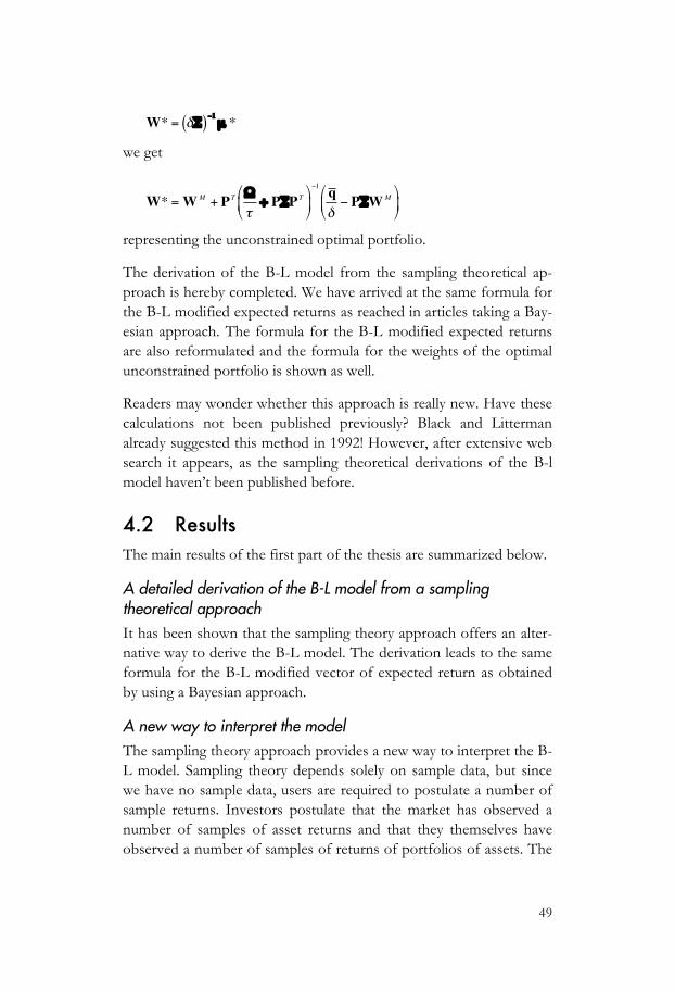
representing the unconstrained optimal portfolio.

The derivation of the B-L model from the sampling theoretical ap-proach is hereby completed. We have arrived at the same formula for the B-L modified expected returns as reached in articles taking a Bay-esian approach. The formula for the B-L modified expected returns are also reformulated and the formula for the weights of the optimal unconstrained portfolio is shown as well.

Readers may wonder whether this approach is really new. Have these calculations not been published previously? Black and Litterman already suggested this method in 1992! However, after extensive web search it appears, as the sampling theoretical derivations of the B-l model haven’t been published before.

4.2 Results The main results of the first part of the thesis are summarized below.

A detailed derivation of the B-L model from a sampling theoretical approach It has been shown that the sampling theory approach offers an alter-native way to derive the B-L model. The derivation leads to the same formula for the B-L modified vector of expected return as obtained by using a Bayesian approach.

A new way to interpret the model The sampling theory approach provides a new way to interpret the B-L model. Sampling theory depends solely on sample data, but since we have no sample data, users are required to postulate a number of sample returns. Investors postulate that the market has observed a number of samples of asset returns and that they themselves have observed a number of samples of returns of portfolios of assets. The

50

number of observations need not be specified, but the number of samples observed by the investor in relation to the number of sam-ples observed by the market must be estimated.

A formula for the parameter

€

τ , the weight-on-views The derivation has generated a formula for

€

τ :

€

τ =nm

It seems possible to interpret the formula. n represents the number of samples observed by the investor and m represents the number of samples observed by the market. Hence,

€

τ is the ratio between these numbers and it is only this ratio that need be estimated. If investors postulate the number of samples they have observed to be the same as the number of samples observed by the market, then

€

τ , should equal 1. If investors postulate the numbers of samples observed by the investor to be more numerous than the number of samples ob-served by the market

€

τ , should be larger than one and vice versa. So, the more confident investors are in all the views, the higher

€

τ ought to be set.

As suggested in chapter 3 it appears that there is no clear description of the variable

€

τ in the existing literature. Hopefully the sampling theory approach presented here will help investors to set

€

τ and help academics as well as practitioners to continue the process of testing and further developing the B-L model.

A new interpretation of the matrix

€

Ω The sampling theory approach to the B-L model generates an inter-pretation of the matrix

€

Ω that differs somewhat from the Bayesian approach. The level-or-unconfidence in an expected return on view i is seen as the value of

€

ω i

2 so that one standard deviation, about 2/3, of the postulated observed samples of a certain view portfolio lies within the interval

€

qi ±ω i . Note that also here investors need not postulate how many samples they have observed, they need only postulate a confidence interval around the expected return of the portfolio so that 2/3 of the postulated samples lie within this interval. It is however possible to implement the model so that investors esti-mate both an interval and another percentage. The investor could

51

then, for instance, claim that he/she believes that in 90% of the n trials, the true return of the view will lie within the interval

€

qi ± γ i .

€

ωi

2 is then calculated from these data.

An inconsistency in the distribution of

€

q j

The distribution of

€

q j is

€

q j ∈ N (Pµ,Ω) , but for the model to be

consistent the distribution should be

€

N (Pµ,P TΣP) . Those trying to understand the B-L model should benefit from knowing of this in-consistency. If unaware it is probable that people will be confused, believing that there is something they have misunderstood. It will probably be easier to handle

€

Ω knowing of this inconsistency.

The reason for deriving the B-L model from a sampling theoretical approach was to facilitate a thorough understanding of the model, both for myself and for others interested in the model. So, is this derivation a contribution in this direction?

It would seem that the results presented above might contribute to a more thorough understanding of the B-L model. New ways of deriv-ing models should constitute a contribution both to academics and practitioners. A derivation of the B-L model from a sampling theo-retical approach hopefully facilitates understanding of the B-L model by individuals not familiar or comfortable with Bayesian theory. The fact that the approach generates an interpretable formula for

€

τ , the weight-on-views, should also contribute to the development of the model. How would it be possible to understand, use, test and/or evaluate a model consisting of one parameter of which no clear and interpretable description exists? However, the practical contribution of this derivation will not be known until it is tested “in use”. Study-ing the use of the B-L model can generate knowledge about how users relate to this way of interpreting the model.

The construction of the B-L model continues and I will continue to take part in this process. The derivation of the sampling theory ap-proach to the B-L model is one contribution to its construction. Since I believe that the contributions are useful I choose to take this interpretation of the model as a starting point in the next step of this thesis.

53

Step II

Behavioural Finance and the B-L Model Having theoretically developed the B-L model and provided a deriva-tion from a sampling theory approach and thereby deepened the understanding of the B-L model, it may seem reasonable to begin doing qualitative case research, as was the idea from the beginning of this project. However, since there is a field researching the behaviour of people facing judgmental issues under uncertainty, i.e. behavioural finance, it seemed reasonable to study the research findings within that field and draw conclusions from research findings from the field to the B-L model.

The aim of the second step is to discuss research results within the field of behavioural finance and their implications in relation to the B-L model. The B-L model is a mathematical portfolio model in-tended for use in portfolio management. Use of the model requires action on the part of its users. Investors are required to make esti-mates and judgments. However, in existing literature concerning the B-L model, there is little discussion of the behaviour of the individu-als or portfolio managers who are supposed to use the model or the context in which the model is to be used. Research concerning the use of quantitative financial models in general and the B-L model in par-ticular appears to be quite limited.

Step II of the thesis will begin with a short presentation of behav-ioural finance. A discussion of behavioural finance in relation to quantitative models in general is then provided before implications from research result from behavioural finance with respect to the B-L model are examined and discussed.

55

5 Behavioural Finance Behavioural finance9 can be seen as a response to the severe criticism levelled at traditional finance theory and the efficient market hypoth-esis (EMH) during recent decades. Many people find the common assumptions regarding homo economicus and efficient markets prob-lematic. Behavioural finance has now become one of the most active fields in today’s economic research (The royal Swedish academy of sciences, 2002).

Behavioural finance is commonly divided into two main parts, as in Barberis and Thaler (2003). One part of behavioural finance is re-ferred to as Limits to arbitrage or Inefficient markets. The other part focuses on the individual investor and the impacts of psychological factors on investment decisions and is commonly divided into two sub parts: The heuristics and biases approach to judgments under uncertainty, and Frame dependence.

9 A more detailed review of the field is provided appendix 3.

56

5.1 The History of Behavioural Finance Camerer and Loewenstein (2004) neatly put behavioural finance, or behavioural economics as the field is also called, in its historic con-text. The following historic description of behavioural finance is based mainly on their article.

The ideas within behavioural finance are not new. Instead they origi-nate from the roots of neoclassical economic theory: “When economics first became identified as a distinct field of study, psychology did not exist as a discipline.” (Camerer & Loewenstein, 2004, p. 4). Many of the well-known early economists, however, had in fact psychological insights. For example, in his book, The Theory of Moral Sentiments, Adam Smith points at the psychological principles of individual behaviour. Ac-cording to Camerer and Loewenstein, many ideas in the book fore-shadow the current developments in behavioural economics. These include Smith’s comment (1759) “we suffer more… when we fall from a better to a worse situation, than we ever enjoy when we rise from a worse to a better”. This is consistent with the concept loss aversion (see appendix 3), one of the major theories within behavioural finance. Jeremy Bentham (1789) developed the utility theory at the end of the eight-eenth-century. Utility theory is the foundation of the neoclassical theory concept, but Bentham also wrote about the psychological support of utility. Some of these insights are now gaining wider ap-preciation.

According to Camerer and Loewenstein, the neoclassical revolution was the beginning of the rejection of academic psychology by ec-onomists. At the beginning of the 20th century, economists such as Irving Fisher and Vilfred Pareto, incorporated discussions about how people feel and think about economic choices in economic theory. In the middle of the century, however, the discussion of psychology had largely disappeared from the economic agenda. At the beginning of the 1960’s the metaphor of the brain as an information-processing device became dominant in cognitive psychology. This metaphor allowed studies of subjects such as memory, problem solving and decision-making. With this, “Psychologists such as Ward Edwards, Duncan Luce, Amos Tversky and Eric Kahneman, began to use economic models as a benchmark against which to contrast their psychological models”(Camerer &

57

Loewenstein, 2004, p. 6). Interest in the field of behavioural finance has expanded tremendously during recent years. This might have to do with the fact that Daniel Kahneman, one of the front figures of the field, was awarded the Bank of Sweden Prize in Economic Sci-ences in Memory of Alfred Nobel in 2002.

5.2 The Parts of Behavioural Finance As mentioned behavioural finance is often divided into two parts; one part concerns markets and the other part concerns individual investors. The part concerning the individual investor is then divided into two different parts. This gives us three areas or parts (Shefrin, 2002):

1. Limits to arbitrage – The efficient market hypothesis states that real-world financial markets are efficient in a sense that prices always reflect fundamental values. In the last 20 years this view of markets has been challenged. The main finding in this part of behavioural finance is that in an economy in which rational and irrational traders10 interact, irrational prices – i.e., prices that differ from their fundamental value – can be significant and long lasting. It is argued that the forces that are supposed to maintain market efficiency, such as arbitrage trading, are likely to be much weaker than the defenders of the hypothesis stress (Shleifer, 2000). Behavioural finance, both theoretically and empirically, offer an alternative approach. See appendix 3 for more information regarding limits to arbitrage.

2a) Heuristics and biases – While limits to arbitrage concerns mar-kets, both “Heuristics and biases” and “Frame dependence” concern the behaviour of the individual investor. Considerable empirical research, within this field, has shown, not surpris-ingly, that people do not always act according to the rational model as suggested by the neoclassical theory. It is worth not-ing is that traditional economists have assumed that the behav-

10 In traditional finance and behavioural finance a rational trader is a trader acting in accordance with the efficient market hypothesis. An irrational trader is hence a trader not acting according to this hypothesis.

58

iour of people differs from the rational model in a non-systematic way and therefore it is considered impossible to in-corporate this behaviour in models. Behavioural finance claims to have found clear systematic patterns in the ways in which people deviate from “rational” behaviour. In 1974 Tversky and Kahneman’s article “Judgment under Uncertainty: Heuristics and Biases” was published in the journal Science. It made a significant impression in the area of social sciences. This was the starting point of the field, within behavioural finance, often referred to as the “Heuristics and biases approach to judgment under uncertainty”. The core idea of the field is that complex probability judg-ments are often based on simplified heuristics instead of for-mal and extensive algorithms, as suggested by the rationality paradigm. This can give rise to series of systematic “errors”11, often referred to as biases. According to the heuristics and biases approach to judgment under uncertainty, people do not estimate likelihood and risk according to the laws of proba-bility. Tversky and Kahneman (1974) present three heuristics: Representativeness, availability, and anchoring and adjustment. Heuristics give rise to a number of biases. Some of the most well established biases are: overconfidence, conservatism, sam-ple size neglect and home bias. See appendix 3 for explanations of the heuristics and biases mentioned here.

2b) Frame Dependence – According to modern finance the fram-ing of a problem should not affect the behaviour of investors. The framing should always be transparent and investors are al-ways assumed not to be affected by how different financial problems are described. However, research within behavioural finance has generated profound results implying that people are sensitive to the framing of problems. Examples of well estab-lished research results concerning frame dependence are: The disposition effect, mental accounting, prospect theory and loss

11 The term “Systematic errors” is used within behavioural finance referring to the systematic divergence of investors from ”rational” behaviour according to homo economicus

59

aversion. See appendix 3 for explanations of these frame de-pendences.

5.3 Behavioural Finance and Quantitative Financial Models

As discussed, behavioural finance, as a field, is a reaction to tradi-tional financial theory. While traditional quantitative financial models assume rational investors, arbitrage-free markets, normally distributed returns etc., research within behavioural finance claims that these assumptions do not apply in the real financial world. People are “irra-tional” (in relation to the assumptions of the efficient market hypoth-esis) in many different ways and this affects how financial models are used and how they should be used.

As mentioned, Limits to arbitrage, claims that the theory of arbitrage-free markets is often inapplicable in the real world. In real life, arbi-trage traders can far from always eliminate what seem to be arbitrage possibilities within the market and hence these “risk arbitrage”12 possibilities can exist in the market for long periods. .

Traditional finance assumes normally distributed returns, but this is a disputed assumption. Discussions about fat tailed13 and skewed14 distributions are common but the normality assumption of returns lies behind many quantitative financial models. Certain research within behavioural finance indicates that returns are not necessarily normally distributed. DeBondt and Thaler (1985) compare two types of stocks: extreme losers and extreme winners. Each year from 1933

12 I choose to refer to these real life arbitrage possibilities as “risk arbitrage”, an expression used by Shleifer (2000). This relates to the fact that real life arbitrage is not risk free.

13 The tails of distributions or returns are often thicker than theory predicts. There are more extreme events, a larger number of very high and very low values.

14 The statistical distribution of returns is not always symmetrical. Frequently the curve shows an asymmetry. This means that it is distorted towards one side, an anomaly compared to the theory.

60

until 1980 they form one portfolio containing stocks with the worst performance during the most recent three years and another portfolio containing stocks that have performed the best during the same pe-riod. For each year they have then computed the returns of the two portfolios over the five following years. On average, the loser port-folio has had higher returns for every period of five years than the winner portfolio. The reason for this, according to DeBondt and Thaler, is that prices overreact. Since investors are likely to extrapo-late past returns into the future, firms becomes undervalued or over-valued. This continues up to a point at which investors begin ques-tioning the market value of the stocks and their price development changes direction. This implies that stock prices are not really nor-mally distributed. They are said to be skewed. Underreaction however suggests that stock prices underreact to information in the short run. According to the efficient-market hypothesis, prices should immedi-ately react “correctly” to new information. However, Abarbanell and Bernard (1992) show that stocks, in general, have higher returns after surprisingly good information than after surprisingly bad information. This also contradicts the normality assumption.

Research results within behavioural finance can be seen as both opposing and supporting the use of quantitative models. Opponents may claim that quantitative financial models are built upon unrealistic assumptions regarding both the investors using them and the mar-kets. Proponents on the other hand may claim that since humans are prone to act “irrationally”, the use of quantitative models may help them to overcome this failing.

Research concerning portfolio models Research has been performed within behavioural finance with respect to portfolio modeling. This research however focuses on how private investors invest their own capital. The research presented here fo-cuses more on how a fund or portfolio manager, managing other people’s money, acts. Shefrin and Statman (2000) present a theory they refer to as behavioural portfolio theory. The theory is not nor-mative as traditional modern portfolio theory but descriptive. Shefrin and Statman discuss how private investors act and how these actions diverge from Markowitz’ portfolio theory. Massa and Simonov (2003) show that behavioural biases affect portfolio choices in different

61

ways. Risk taking, for instance, is argued as being affected by prior gains and losses.

According to Shefrin and Statman, investors divide their wealth into different mental accounts and “construct portfolios as pyramids of assets: cash in the bottom layer, bonds in the middle layer, and stocks in the top layer.” (Shefrin & Statman, 2000, p.149). To each layer they apply different goals with different attitudes towards risk and return. According to the authors, the layer-by-layer style used by investors leads to covari-ances being disregarded. In behavioural portfolio theory the relation between the upside potential and the downside protection is what matters.

62

6 Behavioural Finance and the B-L Model

As explained in chapter 3, the B-L model is a development of the Markowitz model. Two important qualities of the B-L model are that:

The model begins from what is called the equilibrium portfolio, in the literature, most often approximated by the weights of the bench-mark portfolio against which the fund manager is evaluated. This portfolio acts as a point of reference.

The investor inputs “views” and to each view he/she assigns a level-of-unconfidence. The resulting portfolio is then a combination of the benchmark portfolio and the view-portfolio input by the investor. The weighting depends on the levels-of-unconfidence assigned to each view and the weight-on-views.

As argued in chapter 5 most of the research results within behav-ioural finance may have some implication for the use of the B-L model. But, since the above two qualities of the B-L model are the most, important the search for research results within behavioural finance has been focused on research results that might have implica-tions for these two in particular.

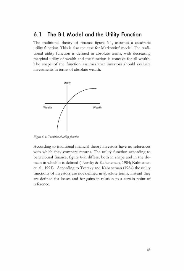
63

6.1 The B-L Model and the Utility Function The traditional theory of finance figure 6-1, assumes a quadratic utility function. This is also the case for Markowitz’ model. The tradi-tional utility function is defined in absolute terms, with decreasing marginal utility of wealth and the function is concave for all wealth. The shape of the function assumes that investors should evaluate investments in terms of absolute wealth.

Figure 6-1: Traditional utility function

According to traditional financial theory investors have no references with which they compare returns. The utility function according to behavioural finance, figure 6-2, differs, both in shape and in the do-main in which it is defined (Tversky & Kahaneman, 1984; Kahneman et. al., 1991). According to Tversky and Kahaneman (1984) the utility functions of investors are not defined in absolute terms, instead they are defined for losses and for gains in relation to a certain point of reference.

Wealth Wealth

Utility

64

Figure 6-2: Utility function suggested in behavioural finance

The function is concave in the domain of gains and convex in the domain of losses. It is also considerably steeper for losses than for gains. The function has a kink at the reference point (origin). The shape of the utility function of behavioural finance implies loss aver-sion15, meaning that the investor is risk-averse in the domain of gains but risk-seeking in the domain of losses.

In the B-L model, the market portfolio acts as a point of reference. This is the portfolio often approximated to the benchmark portfolio against which the portfolio manager is evaluated. If the market port-folio would act as the point of reference it would mean, for example, that if the value of the fund has decreased by 3% in a month while the value of the benchmark portfolio has decreased by 4%, the fund has outperformed the benchmark portfolio and the manager could be satisfied. In traditional finance, a fund manager should be unhappy with a loss and happy with a gain, but according to behavioural fi-nance, the manager rates his or her success relative to a point of re-ference.

15 Loss-aversion expresses the reluctance of people to bet on a fair coin and is im-plied by the kink and the difference in the rake of the value function of prospect theory. Research has shown that the attractiveness of winning X € is not nearly sufficient to compensate for the fear of losing the same amount. Loss aversion how-ever implies that the value function is convex in the domains of losses.

Value

Losses Gains

65

The B-L model builds, as we know, on the Markowitz model. It is thus easily assumed that the utility function of the B-L model should be exactly the same as the utility function in Markowitz’ model. In the B-L model, we optimize a quadratic function, similar to that of the Markowitz model. The shape of the function is hence the same in the B-L model as in Markowitz’ model. There is, however, one important difference between the utility functions of these models. The differ-ence lies in the domains in which the utility functions are defined. The utility function of the B-L model is not defined on total wealth, in absolute terms. Instead the utility function of the B-L model is defined in terms of deviations from a certain point of reference, as losses and gains relative to the benchmark portfolio (market port-folio) in relation to which the investor is evaluated: see figure 6-3.

The utility function assumed within the B-L model can thereby be seen as a step from the traditional, modern finance toward behav-ioural finance. It is defined in domains similar to the domain of the value function of behavioural finance.

Figure 6-3: The B-L utility function

On the other hand, the utility function of the B-L model still has the same shape as that of traditional financial models. It is concave for the whole domain and there is no kink at the reference point. Hence, the utility function does not represent loss-aversion. If the portfolio manager is loss-averse, the bets taken in the portfolio output given by the B-L model in relation to the benchmark portfolio may not neces-

Gain Loss

Utility

66

sarily correspond with that given by the intuitive feelings of the port-folio manager.

The S-shaped utility function of behavioural finance implies that individuals are loss-averse. According to behavioural finance, loss-aversion leads to biases in relation to traditional, modern finance. Biases that seem to be of interest in relation to the utility function of the B-L model are: regret, the status-quo bias, the endowment effect and herd behaviour. These four biases will be presented below and their implications for the B-L model will be discussed.

Regret Much research within the area of behavioural finance has shown that the fear to regret a decision is psychologically strong and influences the decision-making of individuals.

Assume that you have gone with your friends to Nice in France on holiday, planning to spend most of the time at the beach and strolling around in the city shopping and drinking espresso. One day, how-ever, you plan to take the bus up to Grasse to experience the beauti-ful village. The plan has been to leave for Grasse on Thursday, but on Tuesday afternoon the group decides to go on Wednesday instead. So, on Wednesday you all take the buss up to Grasse, but the buss crashes and two of your friends are seriously injured. This would be a very tragic outcome, but is it more tragic because the group originally planned to go the day after? Would you feel any “if only”-thoughts if this had happened to you? Many people find this kind of experience more psychologically painful than if the same accident had happened when keeping to the original plan.

Regret theory (Loomes and Sugden, 1982) and disappointment aversion (Gul, 1991) are both based on the idea that agents value (either in a backward-looking or in a forward-looking manner) the emotional cost of being disappointed and of hav-ing made a mistake, which they might have avoided.

(Stracca, 2002, p. 11)

In prospect theory (Kahneman & Tversky, 1979), the degree of pain of having made a mistake leading to a certain amount of loss is psy-chologically greater than the degree of happiness gained by doing the right thing, which yields a return of the same amount of money. The

67

pain of regret caused by making mistakes is represented by the kink at the reference point in the utility function of behavioural finance (Shiller, 1998, pp. 7-8). When the recall of past experiences is biased, the ability to assess the likelihood that a course of action will lead to a certain outcome is affected. But, decision-making can also be affected even if experience is not biased or when likelihood is not affected. The likelihood might be assessed correctly, but the experience of counterfactual regret can be so psychologically uncomfortable that the action is still avoided (Miller & Taylor, 1995). Odean (1998a) and Shefrin and Statman (1985) have found that to avoid the feeling of regret traders tend to sell winners and hold on to losers. It seems that investors evaluate their original purchase decisions not on the basis of the accrued returns but on the realized return. By selling winners and holding on to losers investors will consider themselves as having made fewer poor decisions. This way of acting facilitates positive self-evaluation since the feedback from losers is delayed.

Numerous studies from a broad range of theoretic fields have shown that regret can affect people’s decision making16. Regret can affect decisions (Shefrin, 2002, p. 31) both when planning a vacation and planning an investment. Even Harry Markowitz admits that he acts according to the unwillingness to feel regret. Markowitz was asked) if his choice of equity-fixed income allocations in a retirement plan was an example of seeking optimum trade-off between risk and return. He answered that this was not the case, instead his intention was to minimize future regret “…so I split my contributions fifty-fifty between bonds and equities” (Shefrin, 2002, p. 31).

The status quo bias and the endowment effect Knetsch and Sinden (1984), Samuelson and Zeckhauser (1988), and Knetsch (1989) introduce the status quo bias.

16 “(Bell, 1982, 1983, 1985a,; Fishburn, 1983; Janis & Mann, 1977; Kahneman & Tversky, 1982a; Loomes, 1988; Loomes & Sugden, 1982, 1987a, 1987b; Simonson, 1992; Sugden, 1985; Walster, Walster, Piliavin, & Schmidt, 1973; see also Gleicher, Boninger, Strathman, Amor, Hetts, and Ahn, 1995)” (Miller and Taylor 1995 p. 379).

68

One implication of loss- aversion is that individuals have a strong tendency to remain at the status quo, because the disad-vantages of leaving it appear larger than the advantages. Samuelson and Zeckhauser (1998) have demonstrated this ef-fect, which they term the status quo bias.

(Kahneman et. al., 1991, pp. 197-198)

Knetsch and Sinden (1984), and Knetsch (1989) demonstrate the status quo bias by randomly handing out mugs and candy bars to students. The students were subsequently given an opportunity to trade mugs for candy. 90% of both the mug owners and the candy bar owners chose not to trade. The authors claim that because the commodities where handed out randomly and transaction costs were low, the preference of the students must depend on the allocation of the commodities. So the commodities that students were allocated were considered as the status quo and very few were willing to leave this position regardless of which commodity they where holding, the mug or the candy bar. In another study by Samuelsons and Zeck-hausers (1998), the subjects where asked a hypothetical multiple-choice question. Some of the subjects had the possibility to choose a status quo answer while others did not. Those not offered the status quo alternative were asked the following question:

You are a serious reader of the financial pages but until recently have had few funds to invest. That is when you inherited a large sum of money from your great-uncle. You are considering dif-ferent portfolios. Your choices are to invest in: a moderate-risk company, a high risk company, treasury bills, municipal bonds.

(Kahneman et. al., 1991, p. 198)

The others were asked a similar question but one alternative was designed with a status quo bias. It could be that the opening sentence was followed by:

…that is when you inherited a portfolio of cash and securities from your great-uncle. A significant portion of this portfolio is invested in a moderate risk company…(The tax and broker commission consequences of any change are insignificant.)

(Kahneman et. al., 1991, p. 198)

The subjects who were presented with a question in which one of the investment alternative was presented as a status quo choice chose this alternative considerably more often than those who were presented

69

with a question with no status quo choice (Kahneman et. al., 1991). In a test carried out by Hartman, Doane and Woo (1990) California electric power consumers were asked about their preferences in ser-vice reliability and rates. The customers were told that their answers would help to determine the future service policy of the company. The consumers fell into two groups. One group of consumers had a much more reliable service contract with the company than the other. Each consumer was asked to state a preferred combination of service and rates among six different combinations. One of the six alterna-tives was always the status quo choice. The test showed that the sta-tus quo choice had a much higher rate of response than the others for both groups of respondents; hence most of the respondents pre-ferred the status quo choice implying that the consumers were status quo biased.

The status-quo bias can, according to Kahneman et. al. (1991) be explained by loss-aversion. Loss-aversion and the status quo bias are closely related to the endowment effect identified by Thaler (1980, 1985). The endowment effect tells us that once a person comes to possess a commodity, he/she instantly values it more than previously (Rabin 1996, p. 5). In an experiment by Tversky and Kahneman (1991), some of the students in a class were given a commodity. The commodity here was also a mug. One third of the students randomly received a mug worth $5. These students where then handed a ques-tionnaire.

You now own the object in your possession. You have the op-tion of selling it at a price, which will be determined later. For each of the possible prices below indicate whether you wish to (x) Sell your object and receive this price; (y) Keep your object and take it home with you....

(Kahneman & Tversky, 1991, p. 145)

The students were also asked to specify their decision at prices rang-ing from $0.50 to $9.50 in steps of 50 cents. The students not receiv-ing a mug were then informed that they would subsequently receive either a mug or an amount of money to be decided later on. They were asked to specify their preference between a mug and an amount of money. These subjects were also to indicate their decision at prices ranging from $0.50 to $9.50 in steps of 50 cents. Here both groups of

70

students face the same decision problem. However their state of re-ference differs. The students receiving a mug at the beginning of the test must chose between keeping the mug and giving up the mug and receiving money instead, hence they must chose between remaining in the status quo or leaving it. The exchange rate between the mug and money was quite different between the two groups. The group receiving the mug at the beginning required $7.00 to give up the mug while the other group felt that they where indifferent between the mug and the money at a rate of $3.50. The difference in the prices depends, according to the authors of the endowment effect, which appears almost directly when individuals are given property rights over consumption goods.

Herd behaviour What happens when each decision maker considers the decision taken by previous decision makers before making their own decision? This is what is often referred to as herd behaviour or herd effects. Consider the following often used explanation for the October 1987 bull market:

The consensus among professional money managers was that price levels were too high – the market was, in their opinion, more likely to go down rather than up. However, few money managers were eager to sell their equity holding. If the market did continue to go up, they were afraid of being perceived as lone fools for missing out on the ride. On the other hand, in the more likely event of a market decline, there would be comfort in numbers – how bad could they look if everybody else had suffered the same fate?

(Scharfstein & Stein, 1990, p. 465)

Denow and Welch (1996, p. 604) claim that there needs to be a co-ordination mechanism for herding to occur. It might be so that be-havioural patterns between individuals are correlated but it might also be so that correlated information arrives independently to investors.

Professional money managers may choose portfolios that are exces-sively close to the benchmark against which they are evaluated to minimize the risk of underperforming this benchmark. Investors may also herd and select stocks that other managers select, to avoid falling behind and losing their reputation (Scharfstein & Stein, 1990). They

71

may also artificially add to their portfolios stocks that have recently done well, and sell stocks that have recently done poorly to look good to investors in connection with fund reports circulated to customers. Pension and mutual fund managers on the average, consistently underperform passive investment strategies (Shleifer, 2000).

Implications for the B-L model The fact that the utility function in the B-L model is defined in the same domain as the behavioural utility function should make port-folios output by the B-L model seem more intuitive to investors. Fund and portfolio managers are often evaluated in relation to a benchmark portfolio and hence often evaluate their own perform-ance in relation to this benchmark portfolio. Since many financial managers are evaluated to a reference point it seems reasonable that the fund manager would appreciate working with a portfolio model taking this reference point into consideration. The taking of bets in relation to benchmark could be one of the reasons why managers find the portfolios generated by the B-L model more realistic than portfolios generated by the Markowitz’ model. If status quo biased, investors should be more comfortable working with a model using the same point of reference, as they are themselves to avoid feeling regret.

However, the shape of the utility function in the B-L model still has the traditional shape of a quadratic function. The bets taken in rela-tion to the benchmark portfolio in the output portfolios will hence probably often differ from the gut feeling of the investor. Regret, the status quo bias, the endowment effect and herding are consequences of loss-aversion. Since loss-aversion is not taken into account in the utility function of the B-L model, expected returns in relation to the risk will not always be high enough for investor to risk leaving the status quo, falling behind the benchmark, feeling regrets and leaving the herd. This implies that portfolios generated by the B-l model also may appear unintuitive to managers, although probably more reason-able than portfolios generated by the Markowitz model.

Since the benchmark portfolio is the point of reference for the fund manager, deviations from this portfolio should generate anxiety. If a bet taken during an investment period proves wrong, it would not be

72

surprising if the manager is subjected to the “if only”-feeling dis-cussed earlier. He/she could easily ask why he took this bet at this particular time and why he/she chose not to keep to the benchmark weights. There has been a recent debate in Sweden about why people pay fund managers the price they charge while holding portfolios very close to the benchmark portfolio. The price a fund charges should be related to the active management and hence the expected excess return provided by the specific fund. Why pay extra for almost no management? The fact that many funds have weights close to the benchmark portfolio might have many explanations. It would be reasonable to believe that the status quo bias might push managers in this direction. Loss aversion may help us to explain this behaviour. Since losses in relation to the reference point have negative psy-chological effects, which are greater than the positive psychological effects of corresponding gains, the status quo bias implies that an investor would frequently prefer to keep to the benchmark weights. Herding and the fear of falling behind in performance should have the same effect.

Now we may ponder upon whether we believe that it would also be better if the shape of the B-L model were similar to the shape of the behavioural utility function. One could argue for this by saying that the portfolio manager would probably not use a model if it contra-dicts his/her intuition. On the other hand, the investor may wish to use a model that helps him/her avoid acting in accordance with his/her biases. I will not discuss this further, leaving the reader with these thoughts, and move on to discussing another important feature of the B-L model in relation to behavioural finance – the level-of-unconfidence.

6.2 The B-L Model and Overconfidence Let us now move on to the other much recognized and interesting idea of the B-L model; the level-of-unconfidence and the weight-on-views. Together, these two factors decide how much weight to allo-cate to the market portfolio in relation to the view-portfolio. There are however considerable research results within behavioural finance indicating that the levels-of-unconfidence expressed by people are often misleading. People are most often overconfident.

73

The following section will begin with a general review of the research on overconfidence and then implications from this research results to the use of the B-L model are discussed and analyzed.

What is overconfidence? A definition of overconfidence is that when estimated probabilities have a tendency to exceed the “accurate portion,” then the judgments on which they are based are said to be overconfident. In behavioural finance, overconfidence relates to the exaggerated belief of people and investors in their ability to correctly forecast returns and future asset prices.

Within behavioural finance and in other fields studying overconfi-dence it is common to discuss two ways in which people tend to be overconfident. Consider two questions of the form:

Which country has the greater population? • Argentina • Egypt

How sure are you that your answer is correct?

In answering such questions, people tend to be overconfident in judging how sure they are of being correct. A typical study, with ques-tions similar to this, has shown that when respondents believe 73% of their answers to be correct, they have actually only answered cor-rectly 65% of the questions asked (Yates et. al., 2002). Another way in which people have been shown to be overconfident is when deeming their confidence interval. Questions testing this can be of the follow-ing form: State an interval of the age of Kofi Annan, so that you are 90% sure that his correct age lies in the interval.

In a study by Klayman et. al. (1999) the correct answers were within the stated interval only 43% of the time when subjects were asked to state an interval in which they were 90% confident their answer lied within the interval. This implies that people are more overconfident when stating confidence intervals than in answering two-choice ques-tions. Many studies have shown that the confidence people assign their judgments exceeds their accuracy. An often-used example of overconfidence is that typically, when asked how good drivers they are relative to other drivers, 65% to 80% of the people answering the question consider themselves as above average. People tend to be

74

overconfident when estimating their own capabilities in many situa-tions. According to Shefrin (2002) investors are as overconfident in their investment decisions as they are in their driving abilities. Over-confidence has been found in several studies to be just as prevalent in the area of finance as in others. 17

People overweight salient information i.e. information that captures attention and stands out (Kahneman & Tversky, 1973). Odean (1998b) claims, that in general we expect people to rely too heavily on less relevant and more attention drawing information and we expect people to underweight important abstract information. Odean also discusses the fact that traders try to invest in assets generating higher returns than others and that this is a quite difficult task. He reminds us that it is in these difficult tasks that people display most overconfi-dence. Odean (1998b) also shows that overconfident investors trade more than “rational investors” and that doing so reduces their ex-pected utility. He models overconfidence, as traders’ belief that their information is more precise than it actually is.

Although an appreciation of overconfidence as an important con-sideration in behavioural finance is well established, research on overconfidence otherwise remains as a subject of debate. Klayman et. al. (1999) suggest that the overconfidence apparently demonstrated by researchers is due to the nature of the questions asked in the ex-periments. The questions are claimed to be harder-than-normal ques-tions. Klayman et. al. (1999) present a study in which they find little general overconfidence in two-choice problems but explicit overcon-fidence in problems requiring the subject to state confidence inter-vals. They find that within easy tasks, overconfidence is not common. Within very simple tasks even underconfidence may appear. The

17 “Examples include psychologists (Oskamp 1965), physicians and nurses (Christen-sen-Szalanski and Bushyhead 1981, Baumannm Deber, and Thompson 1991), engi-neers (Kidd 1970) attorneys (Wagenaar and Keren 1986), negotiators (Neale and Bazerman 1990), entrepreneurs (Cooper, Woo, and Dunkelber 1988), managers (Russo and Schoemaker 1992), investment bankers (Stael von Holstein 1972), and market professionals such as security analysts and economicc forecasters (Ahlers and Lakonishok 1983, Elton, Gruber and Gultekin 1984, Froot and Frankel 1989, DeBondt and Thaler 1990, DeBondt 1991).” (Eric et. al., 1997 p. 8)

75

authors supply two commonly used explanations for overconfidence: biases in information processing and effects of unbiased judgmental error. Early researchers within behavioural finance explained over-confidence with biases in information processing. When a person makes a judgment he/she first searches his/her memory to select a preliminary answer. After this, memory is searched again to find evi-dence supporting the preliminary answer. The retrieval of informa-tion supporting the initial idea is facilitated by mechanisms of associa-tive memory (conservatism) and therefore a person making a judg-ment subconsciously observes more consistent support for the tenta-tive answer than is justified. (Klayman et. al., 1999). The other ex-planation for overconfidence is the effects of unbiased judgmental error. Shortcomings in learning the predictive power of different sources of information are one source of judgmental error considered by Klayman et. al. (1999). According to Klayman et. al. the debate about biased confidence in judgment seemed settled in the 1980s: People appeared to be systematically overconfident in the easiest of questions. In the 1990s overconfidence was given another explan-ation. It was then claimed that people judged questions of confidence imperfectly, but without bias. The questions asked were instead con-sidered to be biased. But in many practical situations many people who are required to make judgments receive biased samples of ques-tions. Doctors, financial managers, lawyers and others are asked ques-tions that are more difficult to answer than questions asked in the world at large. Klayman et. al. (1999) point to the openness of the question of overconfidence, but their study shows, as a large majority of previous studies, that people are overconfident. The more confi-dent they are the more overconfident they are. They also find support for systematism in the way people are overconfident, hence support-ing the concept of overconfidence as a heuristic driven bias.

When are investors overconfident? As mentioned, studies have shown more general overconfidence in estimating confidence intervals than in two-choice questions. Odean (1998b) refers to the extensive research within cognitive psychology, which establishes that people are especially overconfident in judging the precision of their knowledge. As Klayman et. al. (1999) Odean also finds that exceptions to overconfidence can be found when peo-ple are answering very easy questions. He writes that individuals tend

76

to be well-calibrated when asked repetitive questions with fast and clear feedback. When people are asked very easy questions they even can show signs of being underconfident. According to Odean, these exceptions do not, however, apply in financial markets. Traders and investors in the financial markets try to buy assets with higher returns than others and they try to sell assets with lower returns. Odean ar-gues that this is a difficult task and in performing difficult tasks peo-ple are prone to be overconfident. Odean also asserts that security markets are not good places in which to calibrate one’s confidence. Good places in which to calibrate confidence are environments in which feedback is quick and correct. In financial markets, however, feedback is neither quick nor correct. There may also be a trade-off between quick and correct feedback in financial markets. According to Odean, short-term traders may get quicker but noisier feedback while long-term traders get less noisy feedback but must wait for it instead. Research has shown that people overestimate their capability to perform tasks well and that this overestimation increases with the personal importance of the task. People overestimate their own con-tribution to past positive outcomes and underestimate their contribu-tion to past negative outcomes (Odean, 1998b).

Research has shown differences in the overconfidence between groups of people. Gender and cultural differences have been found. Barber and Odean assert:

Psychological research has established that men are more prone to overconfidence than women. Thus, models of investor over-confidence predict that men will trade more and perform worse than women. Using account data for over 35,000 households from a large discount brokerage firm, we analyze the common stock investments of men and women from February 1991 through January 1997. Consistent with the predictions of the overconfidence models, we document that men trade 45 per-cent more than women and earn annual risk-adjusted net re-turns that are 1.4 percent less than those earned by women.

(Barber & Odean, 1998, p. 1)

Yates et. al. (2002) discuss probability judgment across cultures. Wright et. al. (1978) find that Asian students tend to be more over-confident than British students. In the article Yates et. al. summarize what they and others have learned about probability judgments across

77

cultures. They present several studies and almost all of these show that people in western countries (in this case most often USA) are less prone to be overconfident than those in Asian counties.

Wang (2001) takes up the discussion on whether overconfident inves-tors, over time, learn and therefore eventually acquire “rational” be-liefs. He refers to Kahneman et. al. (1982) showing that people actu-ally do not update beliefs and hence do not achieve rationality. Re-search has shown that experience is an important factor in investors’ expectations about the market. The results showed that novice inves-tors are more confident that they will beat the market than the more experienced investors. Since most investors have difficulties beating the market, we have reason to believe that novice investors are often overconfident (Shefrin, 2002). Not only novices exhibit overconfi-dence. Griffin and Tversky (1992) find that when predictability is very low, as in the stock market, experts have theories and models, which they tend to overweight.18

What does overconfidence lead to? Barber and Odean (1999) find that investors who began trading on-line during the period 1991-1996 generally earned less after switching to online trading. When trading over the Internet they increased their trading activity, traded more speculatively and performed less suc-cessfully. Overconfident investors trade more excessively than ra-tional traders. Barber and Odean argue that several biases lead to the overconfidence of online investors. Investors who performed well before going online are likely to attribute this to their own ability instead of luck. Also, online investors get access to data and informa-tion that can give an impression of knowledge, which in turn in-creases overconfidence. The authors also point at the illusion of con-trol investors get when managing their own stock portfolios and can execute a trade with just “a click of a mouse”. This illusion of control also encourages overconfidence. Statman and Thorely (2001) agree with Odean (1998b) in that high returns make investors overconfi-dent and that overconfident investors increase their trading volume.

18 This does not apply to experts who adhere to computer-based quantitative models, see Dawes et. al. (1989).

78

They find strong relations between trading volume and past returns. Shefrin (2002) sees two main implications of investor overconfi-dence. Firstly, investors fail to realize that they are at an informational disadvantage and therefore take on bad bets. Secondly, investors trade too much and therefore reduce their expected utility. Barber and Odean (1999) agree with Shefrin, saying that overconfidence is a simple and powerful explanation for the high levels of trading on financial markets. They claim that humans are overconfident about their abilities, their knowledge and their future prospects.

Odean (1998b) finds that overconfident traders have lower expected utility than well-calibrated traders. It is not so that overconfident traders necessarily have lower expected returns than others. Overcon-fident investors take on a more risky portfolio than would others. It may therefore be so that overconfident investors are rewarded, with higher expected returns, for the extra risk taken. The expected utility, however, is lower. Wang (2001) points at the different views of non-rational traders within financial theory. Black (1986) claims that fi-nancial markets are dependent on noise traders. If all investors were to perceive information in the “correct” way, there would be very little trading in progress since well-informed traders have no interest in trading with each other. Black claims that the financial markets depend on noise traders to provide liquidity in the markets. Friedman (1953), on the other hand, argues that traders who trade on noise are irrelevant to financial markets since they are driven out of the mar-kets by informed investors (in a process of natural selection). Wang (2001) studies whether or not noise traders can survive and especially if overconfident traders survive. He finds that the group of overcon-fident investors survives at the expense of the rational investors. This is because the overconfident investor has a higher expected return than the rational investor and also because he/she has a higher vari-ance i.e. higher risk than the rational investor. This also implies that the overconfident investor, as an individual, is more likely to become a bankrupt, but as a group the overconfident investors survive.

Odean (1998b) takes up what he calls the selection bias and the sur-vivorship bias. The selection bias may cause the financial markets to attract people with a higher degree of overconfidence then the overall population. People differ in their ability to make judgments in situa-

79

tions characterized by uncertainty. Odean claims that those who be-lieve that they have a high ability to make these kinds of judgments will probably seek jobs as traders to a higher degree than others. And, if people are bad at judging their own ability, the financial markets should be populated with those with the most ability and those who are most prone to overestimate their ability. The Survivorship bias, also discussed by Odean (1998b), causes the financial markets to continue to be populated by individuals who are more overconfident than the remainder of the population. Unsuccessful traders lose their jobs or choose to leave the financial market place. Unsuccessful in-vestors will therefore, on an average, manage less money than suc-cessful investors. If investors, to a high degree, as is common, attrib-ute their success as investors to their personal characteristics, they may become increasingly overconfident the more they trade and overconfident investors will control more and more wealth. Gervais and Odean (1997) claim that self-enhancing bias makes wealthy trad-ers, not afraid of being driven out of the marketplace, overconfident. Overconfidence does not make them rich - it is rather the process of becoming wealthy that makes investors overconfident.

Implications of overconfidence to the B-L model Although there is some criticism of the methods used to prove that humans are often prone to overconfidence, overconfidence is still one of the most recognized ideas within behavioural finance. So, if we now accept that people are often overconfident in their judg-ments, does this affect the use of the B-L model?

In the B-L model investors allocate levels-of-unconfidence to each view as explained in chapter 3. A level-of-unconfidence is expressed as an interval around the view-expected-return. With the sampling theoretical interpretation of the B-L model, investors should estimate the interval so that about 2/3 of the postulated observed samples lie within the interval. In the above we have learned that people tend to be overconfident. If people are as poorly calibrated when estimating their own level-of-unconfidence as is claimed, it seems reasonable to question whether the feature in the B-L model that requires investors to input a level-of-unconfidence is such a good idea.

80

Klayman et. al. (1999) claim that people are more prone to overcon-fidence when estimating confidence intervals than in answering two-choice questions. Remember that Klayman et. al. (1999) find that when stating their 90% confidence intervals, the correct answer was only within the interval on 43% occasions. Remember also that this is exactly what the B-L model demand of the investor. The investor must state the 2/3 confidence interval in which the expected return lies. So, when stating these confidence intervals, managers can be expected to assign too narrow confidence intervals.

Research has shown that the overconfidence of a person differs de-pending on the different characteristics of the task. Odean (1998b) observed more overconfidence in the performance of difficult than in easy tasks. Estimating future returns on assets is claimed to be a quite difficult task (Odean, 1998b) and hence people are prone to overcon-fidence in judging their ability to estimate returns. This therefore suggests that people should be overconfident when estimating levels-of-unconfidence in the B-L model. Odean (1998b) also claims that unconfidence levels can be calibrated in situations where feedback is correct and quick, but that feedback in the financial markets is neither correct nor quick, implying that investors act in an environment in which it is difficult to calibrate confidence. The B-L model is in-tended for use in investment situations in financial markets in which people are unable to calibrate their levels-of-unconfidence and hence the users of the B-L model tend to remain overconfident.

The levels-of-unconfidence that should be assigned to views are not the only parameters related to unconfidence in the B-L model.

€

τ , the weight-on-views, must also be considered. The higher weight-on-views is set; the more weight is allocated to the views in relation to the market portfolio or the benchmark portfolio.

€

τ scales the matrix

€

Ω . With the sampling theory approach presented in chapter 4,

€

τ represents the number of samples observed by the investor divided by the number of samples observed by the market. Setting the weight-on-views means neither answering a two-choice problem nor estimating a confidence interval. However, if a person is overconfi-dent when allocating unconfidence levels to each view, it appears probable that investors are also overconfident when allocating the weight-on-views. How well we can estimate future returns, a difficult

81

task according to Odean (1998b), is still dependent on the weight on views. . Hence it seems realistic to believe that investors using the B-L model are prone to express overconfidence both when setting the unconfidence levels to each view and when setting the weight-on-views.

The B-L model is characterized by the way the views of the investors are combined with the market equilibrium or the benchmark port-folio. In this sense the views of the investor are scaled by the weight-on-views. If the investor is equally overconfident in each view, then it is possible to adjust the influence of the unconfidence levels when setting the weight-on-views. The levels-of-unconfidence that the investor must assign have very similar characteristics. They are a measure of the certainty the investor feels with respect to a view. The views can be of different forms as mentioned. They can be abso-lute or relative but all concern the future expected returns of different assets or portfolios of assets. Since the unconfidence levels that should be stated are of similar types, the difficulty of the tasks should be almost the same and hence the extent to which investors are over-confident should also be almost the same. If the investor is as much overconfident in each view, this may be handled when setting the weight-on-views. The levels-of-unconfidence estimated by the inves-tor are tools for ranking the bets taken, in relation to the other bets and to the equilibrium portfolio. Thus if one level-of-unconfidence is biased toward overconfidence and the other levels-of-unconfidences are biased in similar ways, we have at least the possibility of dampen-ing this overconfidence by lowering the weight-on-views, since that

which is actually input to the model is

€

Ωτ

.

The B-L model and home bias Expressing views and levels-of-unconfidence in each view is of course a tool with which users can give expression to many heuristic-driven biases. Since the model provides the portfolio manager with the opportunity to express views and since the model takes these views into account when forming portfolios, the portfolio manager will quite obviously feel that the portfolio output given by the model is more intuitive than the output given by a model not taking these views into consideration.

82

One example of a heuristic-driven bias that can be expressed when using the B-L model is the home bias. Even though the U.S. stock market only capitalizes 45% of the total global stock market, Ameri-can investors still hold most U.S. stocks. In the same way European investors hold mostly European stocks and Japanese investors hold mostly Japanese stocks (Shefrin, 2002, p. 136). Investors might overweight domestic assets because the domestic stocks and markets feel more familiar than the foreign – they are home-biased. Of course investors have more information about domestic assets, but it seems as though they tend to exaggerate this information. Massa and Si-monov (2003) claim that familiarity may depend on either some be-havioural bias or better information about the specific stock. When dependent on a behavioural bias, it is availability or saliency that drives it. Saliency and availability mean that investors focus on infor-mation that is salient or often mentioned even though this informa-tion may not generate any informational advantage in relation to other investors. When underweighting foreign assets depends on an informational disadvantage, the underweighting is of course not a bias (if we do not believe in the strong form of market efficiency). But within the field of behavioural finance the “home bias” is a well-accepted behavioural bias when it comes to investing.

I believe that there are ways in which to act according to the home bias when using the Markowitz model. It seems that investors assume that investment in foreign assets is a risk. Thus when estimating covariances and variances for the Markowitz’ model, the feeling that investing in foreign assets is more risky than domestic investment should be reflected there. Good or bad; this should be the case. Of-ten variances and covariances are estimated from historical data. When estimating covariances and variances in this way the home bias cannot affect the portfolio weights.

In the case of the B-L model, it is possible to increase the estimated risk characteristics of a foreign asset and hence incorporate the home bias as well. But when using the B-L model there is yet another way of incorporating the home bias in the portfolio weights – via the levels-of-unconfidence. It appears reasonable to believe that an inves-tor who is prone to be home biased has less confidence in the views concerning foreign assets than in those concerning domestic assets.

83

Hence, he/she might feel less confident in the views concerning for-eign assets, this leading to the weights in these assets being closer to the benchmark weights than the weights of the domestic assets.

Note that I am not discussing whether this is an advantage or a dis-advantage in using the Black-Litterman model. I am just arguing that it in fact is the case. The B-L model enables home-biased portfolio managers to give expression to this when using the model.

6.3 Behavioural Finance and the B-L Model – What it gave and didn’t give?

The implications drawn from Behavioural finance concern both the attributes that distinguish the B-L model from the Markowitz’ mean-variance model: (1) the equilibrium portfolio as a neutral point of reference and (2) the levels-of-unconfidence together with the weight-on-views. Research within behavioural finance gives support for a reference based portfolio model such as the B-L model. The equilibrium portfolio approximated as the benchmark portfolio seems also to be a reasonable point of reference since this is the port-folio against which the fund or portfolio manager is evaluated. How-ever, with respect to the use of levels-of-unconfidence and the weight-on-views; implications seem more critical. Nothing in behav-ioural finance implies that we should not use parameters to weigh the portfolio weights between the market portfolio and the investor views. But, according to behavioural finance, people have difficulty in estimating their levels-of-unconfidence accurately. They are prone to overconfidence and hence implications from research regarding over-confidence do not favor the use of unconfidence levels when weight-ing between the benchmark portfolio and the view-portfolio.

These implications appear important. They should be useful to an organization considering the use of, or already using the B-L model. However, it should be noticed that these implications are quite indi-vidualistic. They focus on the individual investor and do not take into consideration the social context in which the investor acts. This is actually quite typical of research within behavioural finance. Organi-zational and social questions are ignored. My impression is that researchers within behavioural finance focus on the individual inves-

84

tor as actually being only one single person. In this thesis I have con-sidered the typical investor as a fund- or portfolio manager. Fund- and portfolio managers work most often in an organization and hence they affect and are affected by social and organizational activi-ties in this context. It should also be noted that researchers within the field do not specify limits to their research, which exclude these ques-tions. They express, in fact, no awareness of these issues at all. It is as if they are forgotten, as if the social context in which investors exist has no effect on their professional activities. I consider, as others have previously, this to be a serious omission from research in the field of behavioural finance. Actors on the Financial Markets – an organi-zational finance perspective (Finansmarknadens aktörer – ett organiza-tional finance perspektiv, Blomberg 2005) was published toward the conclusion of this research project. Blomberg criticizes the individu-alistic perspective of behavioural finance, but he also criticizes behav-ioural finance for its structural functionalism. He argues that the indi-vidualism within behavioural finance leads to a reduced possibility to describe and explain complex social processes. The structural func-tionalism within behavioural finance leads, according to Blomberg, to individuals being not only detached from other individuals but also from other structures within the community. I agree with Blomberg. Different social situations should lead to different actions by inves-tors. Hence, the social context and its influences on the actions of the investor seem interesting and relatively unexplored. Another weak-ness in behavioural finance is the lack of real-world studies. Much of the research is performed on aggregated data of different stock prices or empirical material from experiments performed with subjects, often students, making quite unrealistic financial decisions. The sub-jects of these experiments are often students. This is also emphasized by Blomberg (2005).

Does the criticism of behavioural finance suggest that the search for implications from this field for the use of the B-L model has been disappointing? Yes and No! Reading, studying and searching for im-plications to draw from behavioural finance have been rewarding. The implications drawn are both interesting and should be useful when using the model. The limitations of individual actions are still interesting and important when it comes to taking financial decision.

85

Yet, extending the analysis with an organizational perspective seems essential and adds important dimensions.

Frankfurter and McGoun (2002) seriously criticize behavioural fi-nance. In the article Resistance is futile: The Assimilation of Behavioural Finance they claim that behavioural finance, as a field, is being assimi-lated by modern finance. Frankfurter and McGoun make a very ap-pealing analogy with the television series Star Trek in which a crea-ture called the Borg appears. The Borg is a creature consisting of other organisms but acting as one. The Borg aims at development by assimilating other species of the universe into the Borg. Frankfurter and McGoun liken the interaction between behavioural finance and modern finance to the meeting between species and the Borg. When meeting new species the Borg says: “Resistance is Futile. You will be assimilated”. The authors claim that modern finance is now attempting to assimilate behavioural finance in the same way. Behavioural fi-nance has often been referred to as the “anomalies literature”. Now, as behavioural finance gains more and more appreciation, modern finance is no longer trying to exile the field ”to a remote planet”. Instead modern finance is assimilating behavioural finance. Accord-ing to Frankfurter and McGoun this process is retrograde since be-havioural finance is now becoming a prisoner of the forms and meth-ods of modern finance. Adhering too closely to the EMH, they have been unable to establish a new paradigm of finance. What seem to surprise the authors most is that the supposed proponents of the field are in no way resisting the process of assimilation. However, Frankfurter and McGoun provide one explanation of the unresisted assimilation of behavioural finance into modern finance:

Behavioural finance is allowing itself to be assimilated into the modern finance paradigm, because that is the only possible way research can be done today and still be called finance.

(Frankfurter & McGoun, 2002, p. 20)

The individualistic perspective within behavioural finance might have been inherited from modern finance and its future existence might depend on, as Frankfurter and McGoun assert, behavioural finance clinging to the “underlying tenets, forms, and methods of modern finance” (Frankfurter & McGoun, 2002, p. 4).

86

Remember the background of this research project; the project I worked on in 2002, described in appendix 1. Behavioural finance cannot provide tools to analyze the commissioner’s way of acting. To be able to do this we need to move away from the individualistic perspective of behavioural finance and complement the analysis with a social and organizational perspective.

87

Step III

The B-L Model in Practice This third step presents a case study of the B-L model. The first chapter, chapter 7, introduces and outlines step III.

89

7 Introducing Step III The third and final step of the thesis presents an action science in-spired case study concerning the B-L model in practical portfolio management. It presents experiences and reflections on the develop-ment and use of programs implementing the B-L model.

7.1 Input from Step I and II The overall aim of the thesis is to contribute to the development of the B-L model viewed as a tool for portfolio management. So far, the contributions have been of a relatively theoretical nature, nevertheless essential to be able to perform real-world studies of the B-L model.

Step I provided a derivation of the B-L model from a sampling theory approach as well as an interpretable formula to the weight-on-views parameter that had earlier been surrounded with hesitancy and intricacy. Step II provides insights into two of the key features of the B-L model: the levels-of-unconfidence and the weight-on-views. Behavioural finance has shown that most people are overconfident. Estimating confidences is exactly what portfolio managers are sup-posed to do when expressing levels-of-unconfidence to views. There seems to be reason to believe that overconfidence might lead port-folio managers to express too low levels-of-unconfidence and too

90

high weight-on-views. Such knowledge ought to be of importance to anyone working with the B-L model. Research within behavioural finance can also help explain why portfolios generated by the B-L model seem to appeal to portfolio managers: the B-L model uses the same point of reference as is often used by portfolio managers; the benchmark portfolio. Behavioural finance, however, focuses on the individual investor. It seems essential to extend the analysis of the B-L model with a real-world study taking the social and organizational context into account. Such research can add important dimensions to the development of the model.

7.2 Academic Positioning Forslund (2008) divides Scandinavian business administration into four fields: management, accounting, marketing and finance. In all these fields, except to finance, traditions have existed of critical re-search streams such as critical management studies, critical account-ing and critical marketing. These critical streams have also had jour-nals connected to them where such research can be published. How-ever, no tradition has existed of critical finance or journals with such names where critical financial research is published naturally. Forslund (2008) asserts that financial studies with a critical approach have been published in journals associated with critical accounting and critical management studies. Over the last decade, however, re-search with critical approaches to finance has begun to take shape. In this thesis these are referred to as “Alternative finance” (presented in appendix 6). The intention is not to provide a complete description of the research but to show that there do exist financial research streams that take a critical approach towards financial research and emphasize the importance of taking social, cultural and organizational contexts into account, as will be done in this step.

The ways in which alternative finance aims to change financial re-search vary. While some streams within the field are uniting, striving to expand existing financial research, others are more polemic, rather motivated to totally reform the way traditional financial research ought to be performed.

In this step, the existence of several streams of financial research with different ontological and epistemological starting points is considered

91

desirable. One approach need not exclude the other; instead, pluralis-tic perspectives and points of departure ought to be able to generate increased knowledge and better address societal interests.

It should, however, be acknowledged that several individuals with an anti-modernist or post-modernist approach to research who have briefly heard what this research is about and not taken the trouble to engage more deeply in it, have rather quickly interpreted the research as both positivistic and modernistic. As if studying a quantitative model must emerge from a positivistic approach.

Forslund states “a dissertation about financial marketing is different from a dissertation in financial marketing” (Forslund, 2008, pp. 39-40, underlin-ing by the author). Although step III in this thesis is not about mod-ern finance as an academic field, it takes the about approach. It is a study about a model within modern finance. It would probably be problematic to present this kind of research in modern finance jour-nals, since the study is based on action science and interacts with both individuals and organizations, an approach not common in modern finance.

The research has not been steered by alternative finance. There seemed to be a lack of and a need for qualitative, empirical research concerning the B-L model and alternative finance has been drawn upon when performing step III. The research fits well with the over-all call for financial research that is applied and to study the “real world” by actually talking to those involved in what is being re-searched.

The step thereby fulfils the request of Bondio (2003), who maintains the importance of populating abstract financial models with social human creatures. In Bondio’s opinion, writing cultural histories, opening black boxes and thereby showing that markets and money are socially constructed are also of importance to the widening of financial research. While this study does not contain cultural histories it does partly open the black box of the use of the B-L model and brings social creatures into the research. MacKenzie (2005a) says that black boxes are:

92

…devices, practices, or organizations that are opaque to outsid-ers, often because their contents are regarded as ‘technical’.

(MacKenzie, 2005a, p. 555)

He claims that acknowledged expertise can be considered to be a black box and that it needs to be researched to be able to compre-hend how important parts of society are created. Like Bondio (2003), MacKenzie (2005a) claims that the only way of opening a black box is to interact with those involved in its construction.

These arguments fit well with what is done in step III. One aim with this step is to open, at least slightly, the black box of the use of B-L model in practice and this is partly done by interacting with people trying to use the model. Blomberg (2005), MacKenzie (2005a), and Bondio (2003) all point out the importance of holding a construction-ist perspective when performing financial research and such a per-spective is intended to be maintained in all the three steps of this thesis.

My standpoint, however, is that it is not necessary to label this study in more detail than that it draws upon and fits well with the research requested by alternative finance. As Keasey and Hudson (2007) claim:

In essence, there will need to be a concerted effort by those not wedded to the ‘traditional’ finance core to show how an open approach to issues and problems within finance can offer new insights and new research agendas.

(Keasey & Hudson, 2007, p. 947)

Inspiration from alternative finance has had several important effects on step III. It has facilitated keeping an open mind on the empirical material and unexpected issues and not merely to consider B-L spe-cific aspects of the project to be of importance. Alternative finance has also helped me to be more distanced toward the use of the B-L model and enabled me to pay more attention to individuals as well as social and organizational contexts.

93

7.3 Outlining Step III Chapter 8, presents a chronological summary of the work with the B-L model that constitutes the case. It also presents the Wealth Man-agement (WM) group at the Strategic Investment Bank19 (SIB), the organization where the most important parts of the empirical material was collected.

In chapter 9, methodological issues are taken up and discussed. The reason for placing it after chapter 8 is that discussing methodological issues seems more relevant in relation to the case. Action science as a method as well as the empirical material and trustworthiness of the empirical material are taken up in chapter 9. The writing process is presented at the end of the chapter.

Chapters 10 to 13 present the case and reflections on it. Chapters 10 and 11 concern the development of the B-L implementations. Chap-ter 10 takes off from the key features of the B-L model: views, levels-of-unconfidence and weight-on-views. It presents experiences from working with the B-L model and then reflections on the experiences in relation to each feature. Chapter 11 is steered more by the case and considers issues that were not foreseen when beginning the project. The chapter is a result of the openness to the empirical material. Each part of the chapter begins with an empirical description and then reflects on it. Chapter 12 describes and reflects upon the experi-ences from testing the B-L model in real portfolio management situa-tions. Before presenting the results from step III, chapter 13 presents and reflects upon issues of a more organizational character. Results are reviewed in chapter 14. The chapter also briefly characterizes the case and provides an epilogue to step III, commenting on what hap-pened after the research project had ended.

19 The bank’s name is anonymised.

94

8 The Case This chapter provides a summarising chronological description of the carrying through of the case study as well as a presentation of the work of the Wealth Management (WM) group at the Strategic In-vestment Bank (SIB) private banking unit (PB), where important parts of the empirical material were collected.

8.1 Start Up The research project began as long ago as 2005 when together with Tom I started working on a B-L prototype that will be referred to as BLImp (Black-Litterman Implemented). Tom, an engineering physi-cist, owned a consulting firm working with optimization problems and programming. After university studies he had worked increas-ingly with programming quite complex optimization problems. Dur-ing the previous 10 years Tom had mostly carried out assignments for companies in the finance industry and had worked with developing optimization solutions to portfolio problems. We began developing BLImp, which later on became the foundation on which the B-L program for SIB (SIBLImp) was built.

One aim with the development of BLImp was to learn more about using the B-L model. Our hope, however, was to come into contact

95

with a bank or other financial actor that would be interested in using the B-L model with our help. Such a project could provide me with access to a case concerning the use of the B-L model in practical portfolio management.

In November 2006 I met with John at SIB Private Bank for an inter-view concerning the work of portfolio managers. It had come to my knowledge that he and his group, the wealth management group, used a B-L inspired application (from now on referred to as BLOld) in their portfolio management process. John was the chief investment officer (CIO) of the WM group and manager of the group and had held that post since 2003. John was a portfolio manager and had worked as such for the last 20 years. He had no academic background but was very updated and well-read in much financial theory. During the interview John gave a general description of their working pro-cess and their work with the B-L inspired application.

In December the same year I interviewed Pete, a colleague of John. Pete had developed BLOld and had worked at SIB PB since 2005. He was an engineering physicist, but had also taken a couple of courses in financial mathematics. Pete was responsible for the development and the running of BLOld. The interviews with John and Pete were very informative. They spoke frankly about both advantages and disadvantages in their way of working with the B-L model.

In March 2007 Pete gave notice to leave SIB and was to sign off at the beginning of May. John contacted me to ask whether Tom and I would be interested in participating in the handing over of Pete’s program and then engage in helping out with the use of BLOld. This seemed to be an opportunity to access empirical material on the prac-tical use of the B-L model and I therefore accepted to engage in this process. Tom also accepted to participate in the project. This was critical to the ability to perform the study.

8.2 The WM group at SIB Private Banking SIB was one of the most prestigious banks in Sweden. It consisted of five divisions where the private banking division was the smallest.

96

SIB Private Banking was organized into four departments: tax and law, sales, wealth management (WM group) and administration. The major tasks of the WM group, consisting of four people, involved:

1. Responsibility for coordinating all the portfolio management of-fers in SIB PB

2. Responsibility for the discretionary management of the SIB PB including the Dynamically Managed Portfolio (DMP), four Swed-ish model portfolios and a “global long only fund of fund”20

3. Responsibility for all analysis and coordination of analysis in SIB PB. This includes fund analysis, case based analysis of Swedish shares, macro analysis (allocation group), theme investment analy-sis and hedge fund analysis

4. Responsibility for management-related communication such as strategy documents (weekly and monthly), theme analysis, market comments (morning and lunch time)

Since this study concerns the B-L model and the model was only used when managing the DMP, it focuses on the management of the DMP.

Dynamically managed portfolio (DMP) The study deals primarily with the use of the B-L model in the man-agement of the DMP. DMP was an asset allocation fund that allo-cated among different asset classes. The asset classes in which DMP invested were divided into: Swedish Stocks, US stocks, European stocks, Japanese stocks, hedge funds, government bonds, treasury bills and theme investments. Management of DMP was essentially a concept where the WM group allocated up and down the holdings of the various asset classes. DMP was considered to be one product, but was based on three different DMPs: low-risk, high-risk and mid-risk DMP, further on referred to as high, low and mid DMP.

The low, mid and high DMP differed in “riskiness” by holding dif-ferent weights of stocks in relation to fixed income and hedge funds. Figure 8-1 shows a picture of the DMPs and their benchmark

20 A global fund investing in other regular stock funds, hence not hedge funds.

97

weights. The benchmark weights of the mid DMP were 50% stocks, 50% fixed income and hedge funds. The low DMP held less stocks than the mid DMP while the high DMP held more (see figure 8-1 for exact weights). The stock portfolio constituting the asset class “stocks”, however, was the same in all DMPs and held 40% Swedish stocks and 60% foreign stocks as benchmark weights. The WM group had recently changed the benchmark weights of the stock port-folio from 60% Swedish stocks and 40% foreign stocks. John ex-plained that they actually would like to lower the weights in Swedish stocks even more because of the higher risk in the Swedish stock market. This, however, seemed difficult since the customers ex-pressed a desire to hold much of their assets in the Swedish stock market. The portfolio of foreign stocks was divided into US stocks, European stocks and Japanese stocks. The internal relation between the different regions was the same in all the DMPs. The benchmark weights of foreign stocks consisted of 50% US stocks, 35% Euro-pean stocks and 15% Japanese stocks.

The DMP also most often held one or more theme investments. A theme investment was a temporary asset class included in the DMPs. As indicated by the name, theme investments included investments in carefully selected themes. The aim was that the theme investments should exist in the DMPs for quite some time; and they were thus not short-term investments. There could be more than one theme at a time in the asset class and examples of such themes could be infra-structure, environmental, raw material, etc. The benchmark weight of theme investments, however, zero and this is why themes were placed “off-side” in figure 8-1.

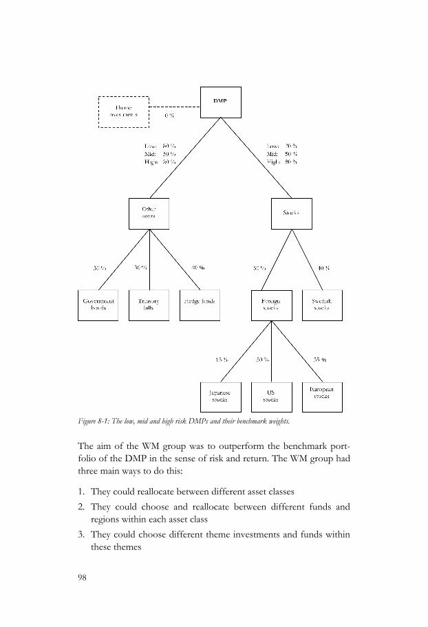
98

Figure 8-1: The low, mid and high risk DMPs and their benchmark weights.

The aim of the WM group was to outperform the benchmark port-folio of the DMP in the sense of risk and return. The WM group had three main ways to do this:

1. They could reallocate between different asset classes

2. They could choose and reallocate between different funds and regions within each asset class

3. They could choose different theme investments and funds within these themes

99

This study focuses on the asset class level and for the most part ig-nores the fund picking process.

The WM group produced monthly and quarterly strategy documents marketed towards customers and internally. In these documents the group presented their analysis of the financial markets. They graded US stocks, Japanese stocks, European stocks, theme investments and stocks vs. fixed income. The grades were on a scale from 1 to 5 where grade 3 represented a neutral view, higher grades positive views and lower grades negative views. I did not take an active part in the process of producing these strategy documents and setting the grades. The WM group, however, asserted that the grades were the results of a thorough analysis process. The analysis process included reading other companies analyses, meeting experts and fund manag-ers and analysing time series and other financial data.

One of the most important and central decisions in the management of the DMPs was the allocation of stocks in relation to fixed income and hedge funds. This decision was not taken by the WM group alone. Instead, a group of “experts” called the allocation committee, in which the WM group had one representative, generated a grade for the stock market. This served as the grade for stock vs. fixed income and hedge funds. The committee consisted of six persons from four countries (Sweden, Finland, Denmark and Luxembourg). Each par-ticipant had expert knowledge in a relevant field such as macro analy-sis, risk analysis, stock analysis, interest rate analysis and asset alloca-tion. The committee held telephone conferences every other week where they, after discussions, agreed on a view on a scale from 1 to 5. A grade 3 represented a neutral view on stocks, 4 or 5 represented a positive view and 1 or 2 a negative view. During the meetings, each member presented their analysis concerning the stock markets, inter-est rates and the overall economic situation and a suggested grade. This often led to discussions, but if the group failed to agree on a grade the chairman had the decisive vote. The meetings were very brief and usually lasted around ten minutes. The grade generated by the asset allocation committee was then used in the strategy docu-ment and as input to the DMP. The grade on stocks not only affected the WM group and its work; it was a standpoint to be held by the whole private bank.

100

Once every quarter the allocation committee made a more thorough analysis of the economic situation. During this analysis they worked with five modules. The modules were:

1. The macroeconomic module to determine were on the business cycle the economy is at the time

2. The leading indicator module to forecast the economy over six to twelve moths

3. The market risk module to estimate the perceived market risk in relation to the historical mean

4. The investor sentiment module to assess the mood of investors with technical analysis, flow of funds and momentum models

5. The valuation module to assess the general price level in the stock market compared to the bond market

These modules produced the grade on stocks.

Hedge funds were included as a separate asset class in January 2008. On average the DMPs were invested in five hedge funds where around half of them were fund of hedge funds. This meant that the asset class hedge funds consisted of around 70-80 hedge funds.

8.3 Implementing During two meetings in May 2007, a couple of weeks before Pete was leaving SIB, he described “the old program” to Tom and me. We received a version of the old program that we could use and study to understand the way it was implemented. BLOld will be presented and discussed further in chapter 10.

Surprisingly little was heard from SIB during the summer and early autumn 2007. Hence, we believed that the use of BLOld went smoothly. I met John for the first time since spring in late October 2007. During the meeting it became clear that SIB had not used BLOld at all when reallocating the DMPs. During the meeting we mostly talked about how they worked before Pete’s departure, about the B-L model in general and BLImp in particular. Later the same day John asked whether Tom and I could demonstrate BLImp a week later.

101

During the demonstration John seemed very positive to BLImp and requested a tender on a start-up project for developing an application similar to BLImp at SIB. On the 17th of December the manager of SIB PB Sweden accepted a budget of 150,000 SEK21 for the imple-mentation of a BLImp for SIB. By that time the project had changed in character. BLOld was left behind. Now the focus was on develop-ing a new B-L application based on BLImp. The version of BLImp developed for SIB PB will from now on be referred to as SIBLImp.

The first step in the development of SIBLImp was for Tom to more or less implement BLImp at SIB and to link correct data to the appli-cation. My main task was to sit down with John and test the applica-tion together with him and analyse how he would like SIBLImp to work. Despite some difficulties and detours, by April 2008 we had developed a version of SIBLImp that was possible to test in real in-vestment situations.

8.4 Case Crisis In early spring 2008 John gave notice to leave SIB, a serious setback for the study and for SIBLImp. So far John had been the only person at SIB engaged in the development of SIBLImp and the enthusiast behind the project.

From the time that John gave notice to leave SIB until he actually left we had two meetings where he tested SIBLImp and John was quite happy with how it worked. When John left SIB, Eric took over as Chief Investment Officer and hence also the management of the DMP. Eric had a degree in economics and business and had started working at the WM group in August 2007 as head of business devel-opment. He worked with John but had more focus on alternative investments and sales. Before working at SIB he had been CIO at two other companies and had had portfolio management responsi-bility for six years.

During spring and summer 2008 no-one worked with SIBLImp. Eric had his hands full with his new role and the loss of and important

21 I had however no monetary claim in this project

102

person in the group. Apart from that, one of the other members of the WM group went on parental leave from June to August. During this time there were also major reorganizations and savings going on at SIB. SIB PB was merged with another, larger organization and the WM group got an additional 12 billion to manage (not in the DMPs however). This resulted in substantial stress on the group, which consisted of only four people. The plan had been to recruit at least two more senior members to the WM group. However, since the whole company needed to cut back, hiring new employees was sud-denly out of the question.

8.5 Testing At the end of August 2008 the WM group decided to reallocate the DMPs. In this reallocation they wanted to test SIBLImp. On 22 Au-gust we ran SIBLImp for the first time since April. Because the group had not had time to get involved in SIBLImp, no-one in the group was familiar with the application at this moment. As a consequence, the testing of the program was much like a demonstration of SIB-LImp.

Eric and Bill were the two persons supposed to use the program from now on. Bill, a fund analyst, had worked for SIB since 2000. Since 2005 he had been working at the WM group and with John. Because of the organizational changes and savings Eric attended internal and external meetings almost all the time and was only engaged in the use of SIBLImp very briefly and sporadically. In September the DMPs were again reallocated and the program was tested once more. The experiences from both the tests are presented and discussed in Chap-ter 12. Figure 8-2 illustrates the proceedings of the project.

103

Figure 8-2: The timeline of step III

104

9 Method The overall aim of the research is to contribute to the development of the B-L model viewed as a tool for portfolio management. The two first steps are of quite theoretical character and lay the founda-tion for empirical research. The aim of the third step is to examine the development and the use of an implementation of the B-L model at a Swedish bank; to discuss and draw conclusions from these ex-periences that can contribute to the development of the B-L model. This is done by a case study at a Swedish bank inspired by action science.

The work of implementing the B-L model constitutes the case. It begins when Tom and I begin to implement BLImp (2005) and ends after two tests of SIBLImp in practical portfolio management situa-tions had been performed (September 2008). The study therefore concerns a case where I, as a researcher, participated in the develop-ment of a computer program implementing the B-L model.

This chapter begins with a presentation of case study research and action science. After the empirical material and the handling of the same are presented, trustworthiness in the empirical material is dis-cussed. The chapter ends by comments on the writing process.

105

9.1 Case Study Research Case study research is well established, especially within the qualita-tive research tradition. Such research has advantages and allows for studies providing “holistic and meaningful contexts to of real-life events” and to understand complex social phenomena (Yin, 2009, p. 4). Case s study research also enables the possibility to study processes instead of results (Merriam, 1998), something that is very much in line with what is done in step III. Yin (2009) says that case study research is appropriate to answer “how” and also “why” questions. Therefore, case studies are appropriate when the desire is to achieve depth and knowledge in the research.

The most common criticism of case study research is the problem of generalizing and of course results from a single case cannot be gener-alised in a statistical way. Yin (2009), however, compares to experi-ments and claims that, like experiments, case studies can be generalis-able to theories although not to populations. Stake (1978) asserts that case study research can be generalised on a personal level. If the re-search is in harmony with the reader’s experiences, the case study may be a “natural basis” for generalisation. Gummesson, however, maintains a quite pragmatic attitude towards the discussion on gener-alising from case studies and means that:

As long as you keep searching for new knowledge and do not believe you have found the ultimate truth but, rather, the best available for the moment, the traditional demand for generaliza-tion becomes less urgent.

(Gummesson, 2000, p. 97)

In the case of the B-L model, a case study has the possibility to gen-erate results concerning model specific characteristics that can only be found when studying the model in practice, such as for instance in what ways the model works well with the reality observed. Deepened understanding of advantages and disadvantages of using the model is also obtainable when doing a case study. Case study research also has the possibility to generate insights concerning the social and organiza-tional context in which the B-L model is used and how this affects its use.

106

9.2 Action Science Research where the researcher takes an active role in the case he or she is studying is treated within qualitative research. This kind of research has different labels: action research (Lewin, 1946) is com-monly used. Other labels are interventionist research (Jönsson & Lukka, 2007), collaborative research (Shani et. al., 2004) and clinical inquiry/research Schein (2001). Gummesson (2000) has been an im-portant source when doing step III. He refrains from using the term action research because of the many projects under this label that have been more of consultancy or journalistic projects and have not met the requirements of scientific work. Also, Gummesson criticizes these projects for using traditional methodologies that originate in the positivistic paradigm. Instead, he uses the label action science and this is the label that will be used in this text when referring to research where the researcher takes action.

Schein (2001, p. 231) argues that such projects often provide empiri-cal material that is deeper and more valid than material collected in researcher initiated projects. Jönssson & Lukka (2005, p. 19) em-phasize the inappropriateness of demanding consultancy fees in ac-tion science projects. No consultancy fee was demanded in this re-search project. Tom, however, who was a consultant and not a re-searcher, charged a fee for his involvement in the development of SIBLImp.

Gummesson (2000, pp. 119-122) states what action science is in ten points. These have served as guidance in this study:

1. “Action science takes action.”

2. “Action science has dual goals: both to contribute to the client and contribute to science.”

3. “Action science is interactive; it requires cooperation between researchers and client personnel and continuous adjustment to new information and new events.”

4. “The understanding developed during an action science project aims at being holistic, recognizing complexities.”

5. “Action science is applicable to the understanding, planning, and implementation of change in business firms and other organiza-tions.”

107

6. “It is essential to understand the ethical framework and norms within which action science is used in a particular project.”

7. “Action science can include all types of data-generating methods but requires the total involvement of the researcher.”

8. “Constructively applied preunderstanding of the corporate envi-ronment and the conditions of business is essential.”

9. “Management action science should preferably be conducted in real time, but retrospective action science is also an option.”

10. “The management action science paradigm requires its own quality criteria.”

Gummesson emphasizes that it is not possible to score high on all the points. Some of them will be commented upon below.

In the second point, Gummesson discusses the dual goals of action science: contributing to both the client and to science. It is important to point out that an action science project actually consists of two different projects (Gummesson, 1991). (1) The core project is the project in which the researcher has a role to contribute to a good outcome for the organization. (2) The research project is the project where the researcher reports experiences and learning from the core project and where he/she also contributes to academic theory. This is an important observation because it is this fact that makes it pos-sible for a failed core project to result in successful research.

In point three, Gummesson claims that action science is an interac-tive process where adaptations to new and changed circumstances must be accepted and welcomed. He emphasizes that it is difficult, if not impossible, to follow a strict research plan. Such a plan may im-pede the research project since the desire to stick to the research plan may prevent the researcher participating in the development of the project. This point has been a challenge in the project where some changes have been possible to accept but hard to welcome. A good example of such a change is when John decided to leave SIB. We were then close to beginning to use SIBLImp and I saw this change as a “threat” to being able to study the use of the model.

The eighth point takes up the importance of preunderstanding. In qualitative research preunderstanding is a debated area and I have chosen to discuss this point more deeply below.

108

Preunderstanding Too much background information and knowledge about the area being studied can have negative implications on qualitative, empirical research. This knowledge may steer the researcher to interpret the empirical data in a specific way. It is therefore not seldom considered an advantage to have little such preunderstanding when performing qualitative research. “Grounded theory” (Glaser & Strauss, 1967) is an example of such a methodology where preunderstanding is seen as something that might be an obstacle when performing empirical re-search (Alvesson & Sköldberg, 2008, p. 157). In critically oriented research Alvesson and Sköldberg (2008, p. 331) argue that theoretical frameworks become more significant. They assert that the theoretical framework can serve as a counterweight to prevent the researcher getting stuck in the empirical material.

According to Gummesson (2000, pp. 79-80) thorough preunder-standing of the corporate environment and of the conditions of busi-ness is important to action science. However, he admits that if know-ledge is closely related to a certain paradigm it may be problematic since research building on such knowledge has a tendency not to distance itself from the theories and methods within that specific paradigm. This kind of knowledge is called blocked preunderstanding (Gummesson 2000, p. 62). There is a risk that the researcher will become biased by knowledge instead of helped by it. The glasses through which the researcher interprets the case are affected by exist-ing knowledge and hence it is possible or probable that some material is ignored and that other material is given too much importance. Gummesson (2000, p. 61) uses a quote from de Bono to illustrate how preunderstanding can block the research:

(it is)…not possible to dig a hole in a different place by digging the same hole deeper. Logic is the tool that is used to dig deep holes deeper and bigger, to make them altogether better holes. But if the hole is in the wrong place, then no amount of im-provement is going to put it in the right place.

(Bono, 1971, p. 22)

If preunderstanding is blocked there is a risk that the researcher will be steered by the paradigm and the comfort it offers. Hence, he or she may try to fit reality into theory instead of the other way around.

109

When performing inductive research, there is a danger that preunder-standing will block or stand in the way of new discoveries. Gummes-son (2000, p. 64), however, claims that it is only in the initial stages of the research that it can be either inductive or deductive. After some time it is inevitable that the researcher jumps back and forth between real world data and theory, often referred to as abductive research. Alvesson & Sköldberg (2008 p. 56) argue that abduction allows theo-retical studies to be used as inspiration in empirical analysis as long as they are not unconsciously applied on the empirical material.

The research process, therefore, alternates between (previous) theory and empirical facts whereby both are successfully re-interpreted in the light of each other.

(Alvesson & Sköldberg, 2009, p. 4)

When the project reported in this study started, I had much back-ground information and knowledge about the area being studied. Theoretically, I had already acquired a deep knowledge about the B-L model during the previous two studies. I also had a good deal of knowledge about the work of a fund manager.22 Have my knowledge and preunderstanding in this case been a burden to the project? My own judgment is that preunderstanding has mainly been an advantage but in some cases also a disadvantage. Had I not had the theoretical knowledge and understanding of the B-L model it seems unlikely that I would have gained access to the project at SIB. In that sense, the preunderstanding was both an advantage and a prerequisite for the study. However, in action science projects the theoretical background knowledge of the research ought often to be the ticket that gives access to empirical material. I do not believe that John would have contacted me if I had not (1) done an interview study with fund man-agers where John was one of the interviewees and not (2) published my licentiate thesis. On the other hand I believe that my preunder-standing has also affected both my actions during the project and my interpretation of the empirical data.

22 From short- time work at two different private banks and one asset management company, an interview study with seven fund managers.

110

Has my preunderstanding been blocked or biased? My endeavour has of course been to try not to let preunderstanding affect the research in a negative way. To lower the risk of being blocked or biased by preunderstanding, I have worked hard to be open to the empirical material. Different researchers, however, treat, interpret and analyse empirical material in different ways. A researcher within traditional finance would, I am sure, generate different results than a researcher within traditional organizational theory would. One endeavour has been to allow the research performed in this dissertation to drift be-tween different research paradigms steered by empirical material. My belief is that this reduces the risk of my preunderstanding affecting this study in a negative way.

9.3 Empirical Material The empirical material from the research project consists of:

• Recorded interviews and meetings: the most important source of empirical material in the study (see appendix 5 for details).

• Four different programs implementing the B-L model: BLOld, BLImp, SIBLImp and SIBLImp(F).

• Printouts from the programs

• Notes from meetings. These mainly concern what was discussed during the meetings, not expressions of people or the physical or social setting of the meetings.

• E-mails.

• My own experiences, learning and insights from the project.

Action science is often associated with research projects concerning organizational change. However, it seems worth underlining that this project concerns the development and testing of B-L implementa-tions, a tool to be used in portfolio allocation. Although the social and organizational context and their effects on the use of the B-L model is very much of interest the main idea is not to analyse the creation of meaning, organizational change or similar. Such research puts other demands on the empirical material and analysis. In this research project I participated in and observed the development of BLImp and SIBLImp but I did not spend as much time at SIB as is usual in traditional action science. However, it is the development

111

and use of B-L implementations that constitutes the case. The devel-opment of BLImp started long before I came into contact with SIB.

The research aims to contribute to the development of the B-L model. It takes an explorative approach and the ways in which the research contributes to the development of the B-L model were therefore not predefined. Instead, the ways that appeared to be the best to continue the process were chosen. The case has steered the research. Although there were some features that were of extra inter-est (the key features of the B-L model) it has been first and foremost what happened during the case that has steered what was to be taken up.

Most interviews and meeting were recorded and transcribed. There are both advantages and disadvantages with recording interviews and meetings (Trost, 2010). My experience is that when taking notes dur-ing an interview or a meeting the conversations are interrupted and disturbed. This has had a negative effect on the meetings and my belief is that these problems would be even more serious in this pro-ject since I am an active member of the meetings and hence partici-pate in discussions quite intensively. Also, my handwriting is slow and bad and it is therefore difficult to use the notes well. Recording inter-views may have a muzzling effect on interviewees. The things dis-cussed during meetings have not however been of such a sensitive nature that I believe this has been a problem. My interpretation is that the participants have spoken quite freely and I believe that quotes will indicate this. However, to enable the participants to speak without worrying about being recorded, at the end of each meeting I have explicitly announced that recording had stopped to enable them to say things that they might not want to be recorded.

To work up the empirical material that the recorded interviews con-stitute they have been transcribed and then analysed using the Hy-perResearch, qualitative analysis software. When coding the tran-scribed meetings both pre-determined codes were used but also codes discovered in the data. The pre-determined codes concerned the main features of the B-L model, i.e. views, levels-of-unconfidence and weight-on-views but also the covariance matrix, an important input to almost all portfolio models. Although these aspects were predetermined, the aim was to keep an open mind, to be open to the

112

empirical material and hence let other aspects of the project be of importance as well. Everything that was perceived as important to the use of the B-L model as a tool in portfolio management was of im-portance, hence the things we chose to do, work with and speak about and the problems we experienced.

The empirical material is of a different character. Recordings and transcriptions constitute an important part of it. Descriptions of what happened during the project have then been written. These narratives are not objective. Instead, I influence them as a researcher and what I have chosen to regard as importance to the research project.

Much of the empirical material consists of recordings from meetings. Already during these meetings, my influence on the empirical material started. And, although the meetings were transcribed almost word for word, some words are always left out or misunderstood. Coughs, background noises, body movements and facial expressions have been left out although these can be of importance. What is presented in this study is hence my interpretation of the empirical material. Another member of the project or another researcher would have interpreted things in different ways. This is often the case in qualita-tive research but may be a more intricate problem in action science. Here, I as a researcher not only affect the interpretation of the project itself, I also affect what actually happened. For a more elaborative discussion concerning subjectivity and interpretation, see Alvesson & Sköldberg (2008).

9.4 Trustworthiness The traditional criteria for evaluating research do not apply when it comes to evaluating qualitative case study research. Following Shah and Corley (2006) other criteria becomes important. They refer to Lincoln and Guba (1985) who maintain that the ambition of qualita-tive research is to create trustworthiness in the empirical material. Trustworthiness is evaluated by four criteria: credibility, transfera-bility, dependability, and confirmability. Inspired by Corley (2004) figure 9-1 presents a table on how these criteria are met up in the third step.

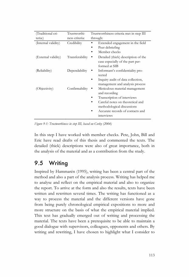
113

(Traditional cri-teria:)

Trustworthi-ness criteria:

Trustworthiness criteria met in step III through:

(Internal validity) Credibility • Extended engagement in the field • Peer debriefing • Member checks

(External validity) Transferability • Detailed (thick) description of the case especially of the part per-formed at SIB

(Reliability) Dependability • Informant’s confidentiality pro-tected

• Inquiry audit of data collection, management and analysis process

(Objectivity) Confirmability • Meticulous material management and recording

• Transcription of interviews • Careful notes on theoretical and

methodological discussions • Accurate records of contacts and

interviews

Figure 9-1: Trustworthiness in step III, based on Corley (2004)

In this step I have worked with member checks. Pete, John, Bill and Eric have read drafts of this thesis and commented the texts. The detailed (thick) descriptions were also of great importance, both in the analysis of the material and as a contribution from the study.

9.5 Writing Inspired by Hammarén (1995), writing has been a central part of the method and also a part of the analysis process. Writing has helped me to analyse and reflect on the empirical material and also to organize the report. To arrive at the form and also the results, texts have been written and rewritten several times. The writing has functioned as a way to process the material and the different versions have gone from being purely chronological empirical expositions to more and more structure on the basis of what the empirical material implied. This text has gradually emerged out of writing and processing the material. The texts have been a prerequisite to be able to maintain a good dialogue with supervisors, colleagues, opponents and others. By writing and rewriting, I have chosen to highlight what I consider to

114

be important and downplay what has seemed to be of less significant for the overall study.

The overall structure of writing has been that presentation of the empirical material is in dated time and describing what happened and what we did and so on. The empirical presentations are often fol-lowed by reflections on the descriptions. Reflections are mainly writ-ten in present time.

115

10 The B-L Features This chapter and chapter 11 concerns the project from start in 2005 until April 2008 when John left SIB. The chapter departure from the three key features of the B-L model: views, levels-of-unconfidence and weight-on-views and analyses these in relation to the three pro-grams implementing the B-L model: BLImp, BLOld and SIBLImp. Investigating these features was predefined when entering the re-search project; hence this chapter takes up issues steered by the model. Chapter 11 on the other hand concerns model issues un-looked-for and is hence more steered by the case.

The chapter takes up one key feature at a time and each section starts with a description of experiences of that specific feature. Afterwards the experiences are discussed and reflected upon.

The reader is assumed to be familiar with the theoretical framework of the B-L model. There is a thorough theoretical review of the model in chapters 3 and 4. Thus, the features are not theoretically defined or explained in this chapter.

116

10.1 Views One of the first things that need to be done when using a B-L model is expressing views23. Views can be expressed both on a relative and on an absolute form and consist of two parts:

1. A view-portfolio specifying which assets that are affected by the view and how much. If for example a view on European vs. US stocks is to be expressed the view-portfolio has 100% in European stocks and -100% in US stocks.24 The weights of a relative view-portfolio typically sum up to 0% while an absolute view-portfolio typically sum up to 100%. Say that the investment universe in European stocks consists of the French and British stock markets then we would like to split the 100% of European stocks to these two asset classes. One way is to just split the 100% and put 50% on the French and 50% on the British stock market. Another way is to estimate the size of these stock markets in relation to each other then maybe it would be more reasonable to put 40% on French stock and 60% in British stocks.

2. The view-expected-return expresses how the user believes the specific view-portfolio is going to return. In the above example with European vs. US stocks the view-expected-return express whether you are positive or negative to this portfolio. Expressing a positive view means that you set the view-expected-return to the view-portfolio higher than the market return25 of that view-portfolio and vice versa.

Views in BLImp The BLImp was kept quite similar to the “original” B-L model, hence similar to the description in chapter 3. The evaluation of the output

23 see chapter 3 for a more theoretical description of views and the parameters view-portfolio and expected return to that view-portfolio.

24 If wishing to express the view as US stocks vs. European stock then the signs would have to be changed and the view-portfolio would have +100% on US stocks and -100% on European stocks.

25 Calculated from the benchmark portfolio

117

of the application was deemed to be easier and more reliable if it didn’t deviate too much from the original model. BLImp was a prototype developed to attract prospects and spending too much effort on developing it seemed excessive. Most of the development was aimed at being done in contact with a user. BLImp was devel-oped just to be able to show interested parties the main features of the B-L model.

BLImp could handle up to six assets. Therefore it was possible to input up to six views, relative or absolute. Setting views in BLImp conformed to the description in chapter 3. To specify a view-portfolio the user created a portfolio with weights representing the view he or she wished to express. The view-expected-return to each view-portfolio then expressed how much the user believed that the specific view-portfolio would return in relation to the market return.

Views in BLOld BLOld worked with fixed view-portfolios (shown in figure 10-1). Hence, the view-portfolios, where already set and the WM group then expressed view-expected-returns to these. It seemed reasonable that the program consisted of these specific view-portfolios because they corresponded well to the way John and the WM group worked. The WM group had worked with these “views” long before they started working with the B-L model. As described in chapter 8 the WM group worked with eight asset classes: Swedish stocks, US stocks, European stocks, Japanese stocks, government bonds, treas-ury bills, hedge funds and theme investments. In the early stages of the project SIB had not yet included hedge funds into the DMPs and hence views concerning hedge funds was never added to BLOld. Theme investments were neither included in BLOld. Government bonds and treasury bills were treated as fixed income and the weight of the portfolio in fixed income was split 50/50 between government bonds and treasury bills. Consequently, the program worked with five views as illustrated in figure 10-1.

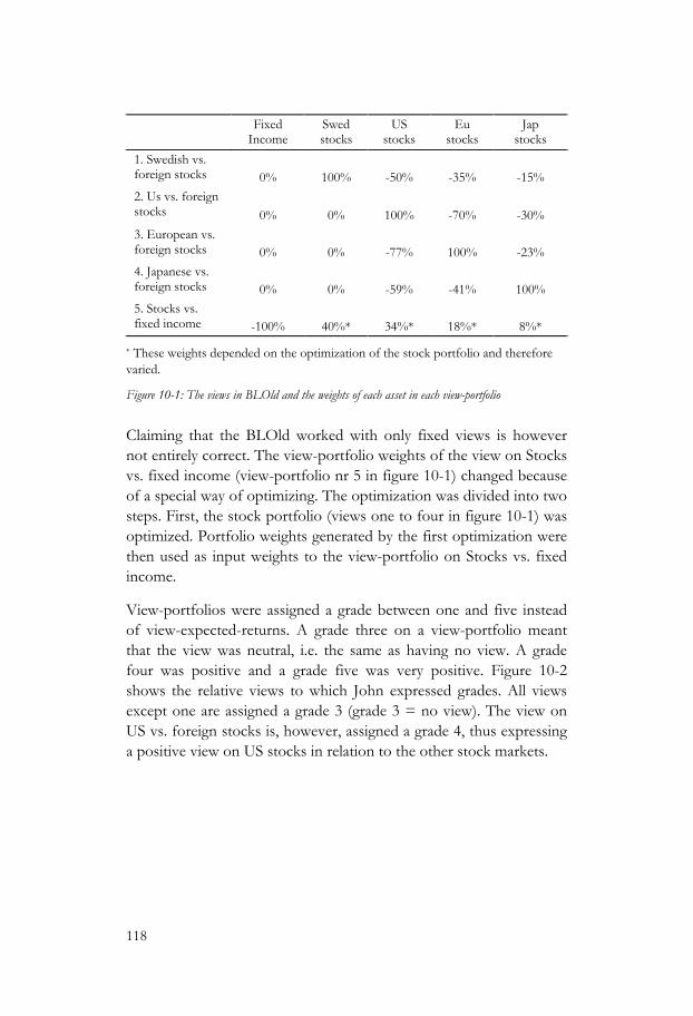
118

Fixed Income

Swed stocks

US stocks

Eu stocks

Jap stocks

1. Swedish vs. foreign stocks 0% 100% -50% -35% -15% 2. Us vs. foreign stocks 0% 0% 100% -70% -30% 3. European vs. foreign stocks 0% 0% -77% 100% -23% 4. Japanese vs. foreign stocks 0% 0% -59% -41% 100% 5. Stocks vs. fixed income -100% 40%* 34%* 18%* 8%*

* These weights depended on the optimization of the stock portfolio and therefore varied.

Figure 10-1: The views in BLOld and the weights of each asset in each view-portfolio

Claiming that the BLOld worked with only fixed views is however not entirely correct. The view-portfolio weights of the view on Stocks vs. fixed income (view-portfolio nr 5 in figure 10-1) changed because of a special way of optimizing. The optimization was divided into two steps. First, the stock portfolio (views one to four in figure 10-1) was optimized. Portfolio weights generated by the first optimization were then used as input weights to the view-portfolio on Stocks vs. fixed income.

View-portfolios were assigned a grade between one and five instead of view-expected-returns. A grade three on a view-portfolio meant that the view was neutral, i.e. the same as having no view. A grade four was positive and a grade five was very positive. Figure 10-2 shows the relative views to which John expressed grades. All views except one are assigned a grade 3 (grade 3 = no view). The view on US vs. foreign stocks is, however, assigned a grade 4, thus expressing a positive view on US stocks in relation to the other stock markets.

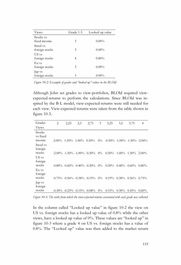
119

Views Grade 1-5 Looked up value Stocks vs fixed income 3 0.00% Swed vs foreign stocks 3 0.00% US vs foreign stocks 4 0.80% Eu vs foreign stocks 3 0.00% Jap vs foreign stocks 3 0.00%

Figure 10-2: Example of grades and “looked up” values in the BLOld

Although John set grades to view-portfolios, BLOld required view-expected-returns to perform the calculations. Since BLOld was in-spired by the B-L model, view-expected-returns were still needed for each view. View-expected-returns were taken from the table shown in figure 10-3.

Grades 2 2,25 2,5 2,75 3 3,25 3,5 3,75 4 Views Stocks vs fixed income 2.00% 1.50% 1.00% 0.50% 0% -0.50% -1.00% -1.50% -2.00% Swed vs foreign stocks -2.00% -1.50% -1.00% -0.50% 0% 0.50% 1.00% 1.50% 2.00% US vs foreign stocks -0.80% -0.60% -0.40% -0.20% 0% 0.20% 0.40% 0.60% 0.80% Eu vs foreign stocks -0.75% -0.56% -0.38% -0.19% 0% 0.19% 0.38% 0.56% 0.75% Jap vs foreign stocks -0.30% -0.23% -0.15% -0.08% 0% 0.15% 0.30% 0.45% 0.60%

Figure 10-3: The table from which the view-expected-returns associated with each grade was collected

In the column called “Looked up value” in figure 10-2 the view on US vs. foreign stocks has a looked up value of 0.8% while the other views, have a looked up value of 0%. These values are “looked up” in figure 10-3 where a grade 4 on US vs. foreign stocks has a value of 0.8%. The “Looked up” value was then added to the market return

120

on the US vs. foreign stocks view and hence the market returns plus the value collected from figure 10-3 constitute the view-expected-return to a view.

The figures in figure 10-3 were calculated “backwards”. The VM group had for a long time used grades on different asset classes to communicate their market views and therefore had data on how much each grade had represented in up or down weighting that spe-cific asset. Suppose that John, as in the above example, had one abso-lute view saying that the US stock market would not outperform other stock markets very much, but still outperform. This view would be represented by a grade 4 on US stocks. Pete then investigated how much this grade had represented in overweight in US stocks earlier. Having estimated how much overweight a grade four on the US stock market had represented Pete calculated the view-expected-return associated with this weight backwards. This was done for each grade represented in figure 10-3.

When we reallocate we have hence chosen a scale from 1 to 5 on each region. If we have chosen a grade 5 on stocks vs. fixed income, how much does that contribute in portfolio weight? I have just looked backward. Ok, this is the amount that it should change, what does that mean to the parameters

(Pete, 2007-05-16)

Views in SIBLImp When first introduced to the idea of expressing view-expected-returns instead of grades to the view-portfolios, John was negative. He felt comfortable using grades in views and believed it to be “sham exact” to set view-expected-returns when forming views. However, after having understood that although it may feel complicated and sham exact to set view-expected-returns instead of grades, BLOld still demands view-expected-returns, John changed his mind.

When development of SIBLImp started, BLImp was first introduced to John. The plan was to let John test BLImp and evaluate how SIB-LImp could work in relation to BLImp. The aim was that John should be able to express what he liked and disliked about working with BLImp and let this information act as input to the development

121

of SIBLImp. In November 2007 John tested BLImp for the first time. He was introduced to the different parts of the program and their intercommunication, tested expressing views and checked the results. After having used BLImp for only a couple of minutes and having tried to set views a couple of times John’s attitude towards using view-expected-returns instead of grades changed. After this meeting he was positive towards this, for him, new way of expressing views.

John was satisfied working with the fixed relative views from BLOld and hence there was no reason to change them in SIBLImp. SIB-LImp thus came to use the same view-portfolios as BLOld except for the view on stock vs. fixed income. At this stage, the reason for divid-ing the optimization into two steps, as was done in BLOld, was not obvious. Fixed weights were therefore used for the view on stocks vs. fixed income in SIBLImp.

Although the WM group managed three DMPs, the low, mid and high DMP, we mainly worked with the mid DMP during the devel-opment of SIBLImp. However, the DMPs had different benchmark weights generating different market returns in SIBLImp. Since view-expected-returns are expressed in relation to market returns, express-ing similar views in the three DMPs became difficult. The view-expected-return to a view needed to be set differently in each DMP. This was a problem we realized but chose to defer and we focused the development of SIBLImp in relation to the use of mid risk DMP.

In the B-L model market returns can be considered neutral returns. If setting the view-expected-return of an absolute view-portfolio equal to the market return, the view should not affect the resulting port-folio. John needed to be able to neutralize relative views and setting view-expected-returns to the same value as the market returns. In the B-L model market returns are calculated to each individual asset and hence to neutralize an absolute view the user sets the view-expected-return portfolio to the same value as the already calculated market return. A relative view, however, concerns several assets and the B-L model does not calculate market returns for such views. The formula for calculating market returns to all views (both relative and absolute) in the SIBLImp was:

122

€

Πviews = PΠ 26

hence multiplying view portfolios with market returns. Market returns were calculated for each view in SIBLImp and thus it seemed to be easy to neutralize the views. But there were more advantages in hav-ing market returns for each view. The market return of a view-portfolio acted as a point of reference when expressing view-expected-return. Hence, setting view-expected-returns larger than the market return implied a positive view and vice versa. John seemed quite satisfied with using market returns as a point of reference when assigning view-expected-return.

Reflections on views Expressing view-portfolios was quite straightforward in the three applications as indicated by the above description. View-portfolios in BLOld were relative and fixed and seemed to represent the views that John wished to express in a reasonable way. These were easily trans-ferred to both SIBLImp and BLImp. At the beginning of the devel-opment, however, we focused on the mid SIBLImp and problems arose when we started to discuss using the SIBLImp for the low and high DMP.

As described earlier, at the time the reasons for dividing the optimiza-tion into two steps as was done in BLOld were not obvious to us. I have since come to realize one advantage in doing so. This relates to the problem of working with several benchmark portfolios, also dis-cussed above. Optimizing in two steps has the advantage that users only need to express one view-expected-return on each view concern-ing only stocks. This is because the stock portfolio is the same in all three DMPs; the only difference is in the weight on stocks in relation to the fixed income. The view concerning stocks vs. fixed income, however, still has to be different in the three DMPs, further discussed in chapter 11.1.

Another difference between BLOld and the other two applications concerned, as explained above, the way the view-expected-returns were expressed. Using grades seemed appealing, collecting the view-

26 For notation see chapter 3.

123

expected-returns from the table in figure 10-3 seemed however a bit peculiar. Pete left SIB already in May 2007 and no one else at SIB knew exactly how the values in the table were calculated. It was thus something of a problem to acquire exact understanding of these fig-ures.

Another problem in using the table in figure 10-3 is that the values, which should correspond to view-expected-returns, are constant. As we know, the view-expected-returns are added to the market return. The market return on a specific view-portfolio is not constant but changes over time. The market returns depend, for instance, on the covariances between the returns on the assets and they are not con-stant. If John, as in the example in figure 10-2 above, had a view rep-resenting a grade four on US versus foreign stocks this would always correspond to adding 0.8% to the market return regardless of the value of the market return on that specific “day”. Hence, adding for example 0.8% to a low market return would influence the output portfolio more in a positive direction than the same view-expected-return would on a high market return. This must therefore be seen as a problem with BLOld.

As can be seen from figure 10-3, some grades have no value assigned to them. This is due to the fact that during the time the WM group had used BLOld (from March 2006 to April 2007) they had only had views with grades between 2 to 4, never 1 or 5. They had not had such strong views that would allow for such a strong positive or negative grade. However, they used half grades and even sometimes quarter grades, which can be seen as deviation from a five-graded scale.

As described, John was at first reluctant to express view-expected-returns instead of grades. However, he almost immediately changed his mind after having tested expressing view-expected-returns in SIB-LImp. One reason why John changed his mind may depend on his willingness to use an implementation closer to the “original” B-L model and felt that setting view-expected-returns instead of grades would contribute to this. It should, however, be said that Tom and I recommended John to use view-expected-returns instead of grades and this probably had some effect as well.

124

The B-L literature (for example Black & Litterman, 1992 and Gia-cometti et. al., 2007) only presents a formula for calculating market returns to absolute views. However, SIBLImp used relative views and expressing view-expected-returns for these was difficult without mar-ket returns. Calculating market returns for relative views was nothing revolutionary but nevertheless helpful.

Early in the work with SIBLImp, John made it clear that he intended to develop his knowledge and understanding of the theoretical char-acteristics of the B-L model quite thoroughly. One reason for doing so was to be able to explain it to customers. But a more important reason was that he needed to explain it to the relationship managers at SIB PB (discussed further in chapter 13.1). To me it was gratifying that John wished to understand the theoretical characteristics of the model since a point of departure in this thesis is that understanding is important when using the B-L model. To help John acquire a deeper understanding of the B-L model I was careful to explain the different features of the model. One of the reasons for suggesting using view-expected-returns instead of grades in SIBLImp was that I believed it would help John to better understand both the B-L model and the specific implementation of SIBLImp. I explained in detail how to specify view-portfolios in SIBLImp to provide the possibility to deepen the understanding of the model. However, since we chose to use the fixed, relative views, my endeavour to explain to John exactly how a view was built might actually have impeded his understanding instead of the other way around. SIBLImp may have appeared more complicated to use than necessary. To use SIBLImp John did not have to express view-portfolios since they were already stated in the application. He only needed to set view-expected-returns to those view-portfolios where he had opinions. The complex appearance of the SIBLImp might have deterred John from actually testing the pro-gram for himself, something that he often mentioned he needed to do to be able to evaluate it. Unfortunately, John never found time to test the application alone.

125

10.2 Levels-of-unconfidence After having expressed a view, a level-of-unconfidence27 should be assigned to that view. The possibility to express levels-of-unconfidence to views is considered an important feature of the B-L model. There are, however, problems associated with this feature theoretically. There are hence reasons to believe that this also is the case when expressing it in practice.

Levels-of-unconfidence in BLImp The traditional way of expressing levels-of-unconfidence for a view in the B-L model is in the form of standard deviations or variations around view-expected-returns. Alternative ways can, however, be found in the literature. One idea has been to express confidence as percentages (Idzorek, 2004). Another way is to express confidence as grades for each view (Bevan & Winkelman, 1998). It should be em-phasized that both these “alternative” ways of expressing confidence use the standard deviations or variances in the calculations; the rest are “build-ins” to facilitate the use of the model. Setting levels-of-unconfidence as percentages or as grades seemed appealing when developing BLImp. For users not that familiar with the B-L model or statistical analysis, it would probably have been intuitive. Neverthe-less, although some users might find it difficult to set levels-of-unconfidence as standard deviations around view-expected-returns this was the way the feature was implemented in BLImp. The aim was, as when implementing the view feature, to keep BLImp close to the common interpretation of the B-L model. The testing of BLImp also seemed to be more straightforward this way. Another reason for using standard deviations was the fact that BLImp was a prototype developed while trying to find a user in practice. We intended to let future users steer the development of their application. However, many financial actors and portfolio managers are quite used to work-ing with standard deviations in relation to risk and it seemed reason-able that they might have a general feeling for the parameter.

27 See chapter 3 for a theoretical description of levels of unconfidence

126

When testing BLImp, difficulties arose however in deciding the ap-proximate size of the levels-of-unconfidence i.e. the standard devi-ations. A level-of-unconfidence is closely related to the view-expected-return and so is the weight-on-views. These three variables interact and affect how much the weight of a specific asset in the output portfolio deviates from the benchmark weight. It was there-fore problematic to know which variable to set to which value. To facilitate the setting of the level-of-unconfidence, a kind of reference level-of-unconfidence was calculated. We called this variable the “market level-of-unconfidence”. The market level-of-unconfidence is in the following called yi.

€

yi = PiΣPiT 28

hence, the standard deviation of view portfolio i. Idzorek (2004) sug-gests using this value as level-of-unconfidence whereas we chose to use it as a point of reference. Using the market level-of-unconfidence as reference made it easier to express levels-of-unconfidence. How-ever, we still did not perceive the parameter as unproblematic. What does it mean to be more secure than the market and what value does my confidence represent?

Levels-of-unconfidence in BLOld In BLOld, the levels-of-unconfidence were not implemented. In-stead, all the levels-of-unconfidence were set to a constant and the user did not specify it. The level-of-unconfidence was set to 0.0005, which might be considered a surprisingly low value. When discussing with Pete why he chose this value one of his comments was:

Omega, I just sat like a diagonal matrix with any value that made it (BLOld) change appropriately.

(Pete, 2007-05-16, parenthesis by the author)

He was hence not aware of the value of the levels-of-unconfidence in BLOld. In Pete’s opinion, he had calibrated the model so that it gave reasonable output.

28 For notation see chapter 3.

127

…and if I could get this to work in a better way by choosing better values on tau and omega I would, but it is nothing that I have spent time on.

(Pete, 2006-12-13)

Setting the levels-of-unconfidence to 0.0005 was hence a way to cali-brate the application. To make the application output portfolios that Pete and John felt were reasonable the levels-of-unconfidence needed to be set to such a small value.

Pete motivated the fact that they did not use the levels-of-unconfidence by relating to the number of parameters (aiming at view-expected-return, level-of-unconfidence, weight-on-views) to which the user needed to assign values. In his opinion, there was a risk that the application would become too complicated, at least to start with. Pete explained:

I like the theory and the basic idea of the model (B-L model) that is so easy to understand but the confidence matrix is more of a bonus that you can use in the future and then I don’t care how I set either omega (level-of-unconfidence) or tau (weight-on-views).

(Pete, 2006-12-13, parenthesis by the author)

As presented above, the level-of-unconfidence for each view was set to a constant value in BLOld. It was surprising, to us, that SIB chose not to use levels-of-unconfidence sine it is one of the key features of the B-L model. What was even more surprising, however, was that John believed that the levels-of-unconfidence were used and even set levels-of-unconfidence continuously. When it was pointed out to John that the levels-of-unconfidence were not used in the program, he answered:

But we have done that all the time

(John, 2007-10-23)

Checking again both with the transcribed meeting (2007-05-16) and BLOld and with Tom, my first belief was confirmed. In BLOld lev-els-of-unconfidence were in fact not used. John set levels-of-unconfidence but these were not input to BLOld.

128

Levels-of-unconfidence in SIBLImp As mentioned in chapter 10.1 John had been quite reluctant to stop working with grades when setting view-expected-returns. He was also negative to expressing levels-of-unconfidence as standard deviations instead of grades, as he had done (although they had never entered BLOld). During a meeting in November 2007 when testing BLImp he nevertheless changed his mind and wished to work with view-expected-returns and standard deviations instead of grades.

Tom and I had for some time discussed the possibility of letting users evaluate their confidence with the help of SIBLImp. By measuring how often the actual return of a view fell outside the interval speci-fied by the level-of-unconfidence, confidence could be evaluated. If the user were well calibrated the actual return should fall outside the interval two thirds of the times. If the actual return fell outside the interval, more often it would indicate an overconfident user and vice versa for underconfidence. During the development process, John often expressed a desire to “get better”. Developing a better model was one way. Another way was to understand the B-L model more deeply. When introduced to the idea of evaluating his confidence, John was excited and believed this to be a very interesting idea that he defi-nitely wanted to use. We agreed that this feature would be developed in the next version of SIBLImp.

Reflections on levels-of-unconfidence Experiences from the case indicate that expressing a level-of-unconfidence is not trivial. The impression is that neither Pete nor John had acquired deep understanding concerning this parameter. This is not surprising because it seems difficult to acquire deep understanding of the levels-of-unconfidence without both understand-ing the theory and using the feature in practice. It should be noted that although I had quite deep theoretical understanding of the levels-of-unconfidence and had also tested BLImp, and thus used the lev-els-of-unconfidence in practice, I still found it difficult to set the values. In BLOld the problem was solved by not using the param-eter. Interestingly, John believed they used the levels-of-unconfidence and expressed his confidence continuously, although in grades in-stead of standard deviations.

129

My impression, however, is that Pete did not strive to implement the B-L model in its essence. Instead, he wished to develop a B-L in-spired application that was not too difficult to use and output port-folios that seemed reasonable, intuitive and in line with the views set. Pete calibrated the different parameters to make the application be-have in a desired way. If the program acted strangely it was just to check why it behaved in this way and then calibrate it to make it work well in that specific situation. Since the portfolio was supposed to “seem reasonable” Pete ought to have had some kind of reference portfolio to relate to, a portfolio that the output from BLOld could seem unreasonable in relation to. Pete’s reasoning concerning cali-brating BLOld, however, points to a problem with the B-L model. To use the B-L model, several parameters need to be set and these pa-rameters interact. If, for example, a view is set with a high view-expected-return in relation to the market return, the influence of that view-expected-return can be dampened by a high level-of-unconfidence. It is also possible to increase or decrease the influence of a view on the output portfolio once more by setting a high or low weight-on-views. When using neither levels-of-unconfidence nor weight-on-views but instead setting them as constants, it is possible to set such seemingly “unrealistic” values and still get realistic results because of the other parameters that affect the output portfolio.

As described, Tom and I agreed to let levels-of-unconfidence be expressed as standard deviations when working with BLImp. In addi-tion, in SIBLImp we used standard deviations to express levels-of-unconfidence. Retrospectively, I have come to question this decision. It might have contributed to make the application seem complicated and therefore been an obstacle to John actually test-running the model on his own. During the development of SIBLImp John often said that he needed to sit down and test SIBLImp by himself to de-velop a better understanding and evaluate whether he liked the way the application worked or not.

I need to simulate enough so that I understand. To see that it does what I expect it to. Hence it is a model that is supposed to do what you expect it to do.

(John, 2007-11-08)

130

I should have tested a bit more before but I don’t know if there will be time maybe next week or perhaps on Friday.

(John, 2007-12-12)

No, but you must surely learn to play with it so that you under-stand its sensitivity.

(John, 2008-04-24)

He was almost always positive to our ideas and suggestions but pointed out that he needed to find time to sit down with SIBLImp to test it. The intention was to develop SIBLImp in close relation with the user. However,, John actually never tested using SIBLImp or BLImp on his own. We showed him SIBLImp several times and he tested it with us and gave feedback but he never tested it on his own in peace and quiet to evaluate its different features. It therefore seems reasonable to wonder whether using SIBLImp might have seemed too complicated.

Evaluating why John did not test-run the model as he so often said, has made me come to understand Pete’s arguments for not imple-menting levels-of-unconfidence in BLOld. In Pete’s opinion, imple-menting the levels-of-unconfidence would make the program too complex to use. However, John actually estimated his confidence, believing that this parameter entered BLOld although it did not. Hence, getting John to express levels-of-unconfidence was not the problem here. However, setting them as standard deviations instead of grades might have contributed to make SIBLImp seem complex. During the development of SIBLImp, John expressed a wish to understand and learn more about the B-L model. This and the fact that he actually already set levels-of-unconfidence (they just did not enter BLOld) supported using levels-of-unconfidence in SIBLImp.

We tried to facilitate the use of the levels-of-unconfidence in SIB-LImp by calculating the market levels-of-unconfidence, as described above. Market levels-of-unconfidence seemed to generate a useful point of reference when setting levels-of-unconfidence. John related to this parameter when expressing the levels-of-unconfidence.

As described in chapter 6.2 implications from research within behav-ioural finance emphasize that people in general experience great diffi-culties in judging their own confidence (Klayman et. al., (1999), Bar-

131

ber & Odean (1999), Gervais & Odean (2001), Griffin & Tversky (1992), Odean (1998b), Shefrin (2002), Statman & Thorely (2001) and Wang (2001)). People tend to be overconfident in their ability to estimate future events. People who are overconfident in their ability ought also to be overconfident when estimating levels-of-unconfidence, especially since estimating these means estimating a confidence interval, a type of confidence estimate that has proved to generate much overconfidence. There therefore seemed to be prob-lems connected to expressing levels-of-unconfidence to the B-L model.

It is not only our inability to judge our confidence levels that seems problematic. Expressing the level-of-unconfidence for a view can be divided into two steps. First, the user must try to estimate how sure he or she is about a view. It is in this step people tend to be overcon-fident and believe they are more sure than they have reason to be. The second step is to convert the perceived level of certainty to a standard deviation around the view-expected-return. Although John quite quickly changed from wanting to work with grades to wanting to work with standard deviations, we found it quite difficult to esti-mate an actual standard deviation that fitted well with the perceived level of certitude, overconfident or not. How we set the levels-of-unconfidence will be discussed further in chapter 12.

As described earlier, we decided to implement a feature so that a user of SIBLImp could evaluate his or her own confidence. Although research within behavioural finance indicates that it is difficult to calibrate confidence (Odean, 1998b) such a feature ought still to be useful. If your level-of-unconfidence is constantly set too low it seems as if you are overconfident. Knowing this may have an effect on the user when setting levels-of-unconfidence in the future. John also showed great interests in such a feature.

A challenge for John was that he was supposed to handle and run SIBLImp by himself. BLOld was developed and handled by Pete alone, John handed over views to Pete that he input to the applica-tion. If the resulting portfolios seemed strange in any way it was dis-cussed with John but John didn’t actually use BLOld. Therefore the step just to sit down with a program was a big step in this project and this was a step that Tom and I didn’t reflect much about during the

132

development of SIBLImp. If the data input to SIBLImp would have been more similar to the way they were expressed in BLOld it seems reasonable that the step to sit down with the program would have been smaller. It should however be noted here that all the changes taken up so far were discussed with and approved by John in fore-hand.

10.3 Weight-on-views Weight-on-views, presented theoretically in chapter 3 and 4, is an-other parameter influencing how much the output portfolio from the B-L model deviates from the benchmark portfolio. It scales the weights of all the views in relation to the benchmark portfolio. We can say that weight-on-views scales up or down all levels-of-unconfidence.

Weight-on-views in BLImp, BLOld and SIBLImp When developing BLImp weight-on-views was set to one. Setting the parameter to one and keeping it that way implies that it is neutralized and not used. This was done because of the many parameters that interrelate in the B-L model and it seemed difficult to use all of them at the outset. Weight-on-views, however, was not assumed to be a useless parameter. It was just the parameter that was easiest and most reasonable to ”put on hold” when trying to use the B-L model in practice. In SIBLImp the same approach was used. It seemed reason-able to let users develop an understanding of how to set views and levels-of-unconfidence first.

In BLOld weight-on-views was set as a constant in the same way as the levels-of-unconfidence. It was, however, not set to 1 so the pa-rameter was not neutralized. Instead, it was set to 0.0025. A valid explanation why this value was chosen was never retrieved and nei-ther was a reason why levels-of-unconfidence were set to 0.0005. It seemed as if Pete did not know to what values these parameters were set.

Depending on how you set tau (weight-on-views) it doesn’t matter. I think I have set it to one or something.

(Pete, 20007-05-16, parenthesis by the author)

133

However, as mentioned above, he calibrated the model to output reasonable results and these were the values on weight-on-views and levels-of-unconfidence he ended up with.

Reflections on weight-on-views As mentioned earlier, several parameters in the model interrelate, making it difficult to understand how to set each parameter. In par-ticular, levels-of-unconfidence and weight-on-views interrelate and weight-on-views can be interpreted as scaling up or down all the lev-els-of-unconfidence.

The formula for the B-L view-expected-returns (see chapter 3 and 4) can be expressed as:

€

µ* = Π + ΣPT Ωτ

+ PΣPT

−1

q − PΠ( )

where

€

Ω represents the diagonal matrix containing the squared lev-els-of-unconfidence and

€

τ represents the weight-on-views. Hence, only the quotient between the levels-of-unconfidence and weight-on-views enters the B-L model. Since the levels-of-unconfidence are constant and the same in all views in BLOld, the value that enters the model is the quotient between 0.0005 and 0.0025, i.e. 0.2. The strangely small numbers therefore are not that puzzling. BLOld would have acted in the same way as long as the quotient between these two parameters was 0.2. This elucidates the difficulty in discuss-ing the values of the different parameters in the B-L model separately – they interrelate.

How Pete ended up with the specific figures 0.0005 on levels-of-unconfidence and 0.0025 on weight-on-views is still not obvious. My belief, however, is that they have started with some figures and then tested the model and adjusted the figures to make BLOld behave in a reasonable manner. It seems, however, that it would have been more intuitively to set weight-on-views to one and the levels-of-unconfidence to 0.2. In this way the weight-on-views parameter would have been neutralized.

134

10.4 Conclusions: The B-L Features The experiences from working with the B-L implementations (BLImp, BLOld and SIBLImp) indicate that levels-of-unconfidence are quite intricate to express. When developing both the BLImp and the SIBLImp we experienced difficulties in estimating the size of this parameter. The difficulty was, in some way, handled by using market levels-of-unconfidence as a point of reference.

Important knowledge includes how the three key features interrelate. The way they interact contributes to the difficulties in determining the approximate size. However, setting weight-on-views to one, as was done when developing the SIBLImp, seems reasonable. The parameter is therefore temporarily excluded. The approximate size of the view-expected-return is generated by the market returns. Calculat-ing the market levels-of-unconfidence, as was done in the SIBLImp, to get a reference level to this parameter, provides guidance regarding its level. An understanding of the interrelations of the parameters is a consequence of the first step of this thesis. That step generated understanding of the theoretical characteristics of the model. Build-ing-in the possibility to evaluate levels-of-unconfidence seems appeal-ing.

The chapter provides a thick description concerning the work with the B-L model. One experience, that will be developed further in chapter 13.3, is both the importance of and the difficulty in getting users involved in the development process. In this case, John was quite committed to the development of the SIBLImp, it was he who had contacted me and Tom to help him to use a B-L model. Never-theless, he never found time to test the programs seriously. Consider-ing the difficulties we had in engaging John in the development of a tool of which he himself actually was the initiator, it is not hard to imagine the difficulties of getting users engaged in the development of a tool that they have not asked for. John was the driving force of the project and the SIBLImp. When he left SIB the development of the SIBLImp was put on hold. 29

29 The importance of individual enthusiasts is discussed in relation to the development and implementation of Business Intelligence systems (Borking et. al., 2009, p. 15).

135

11 Model Issues Unlooked-for While the previous chapter concerns the key features of the B-L model this chapter is guided by model issues unlooked-for, but that had significant impact on the development of the B-L tools. The chapter is structured as the previous one. Each issue is presented in its own section; the first part describes of what happened and these undertakings are then discussed and reflected upon.

11.1 Several Benchmark Portfolios In 2006-2007, before the contact with SIB, Tom and I had a dialogue with another bank to develop a B-L implementation. The project ended before an agreement could be reached. However, a sketch of a solution to their situation was made. The bank was a small, newly started private bank. Every customer had his or her own, personal benchmark portfolio. The benchmark portfolio was decided together with the client. Differences in the benchmark portfolios depended on the customers’ wiliness to take on risk, the length of his or her in-vestment horizon and the customers’ specific wish to hold or not hold certain assets in the portfolio. Some customers had only stocks in their portfolio while others had stocks, bonds, commodities and more.

136

The disparity of benchmark portfolios resulted in problems when trying to apply the B-L model. The portfolio manager only wanted to express one set of views that could be used for all customer port-folios. However, since each customer had an individual benchmark portfolio, market returns resulting from these differed (since the market return is dependent on the weights of the benchmark port-folio, see chapter 3). And, since view-expected-returns should be expressed in relation to market returns, a certain view could be posi-tive in one portfolio while negative in another. To get the same influ-ence from views in all portfolios, the manager would have to express different views for each customer portfolio. Working in this way seemed difficult, if not to say impossible. If the portfolio manager manages a substantial number of portfolios, say 250, it would be un-realistically time-consuming to set views for every portfolio.

As mentioned in chapter 10, a similar problem was dealt with during the development of SIBLImp. However, it was not of the same mag-nitude since the WM group did not work with individual benchmark portfolios for each client. Instead, a customer was slotted into one of three different portfolios with different risk profiles (low, mid and high DMP), each having its own specific benchmark portfolio. This resulted in different market returns for each DMP and for the view-expected-returns to influence the portfolio holdings in the same way, they therefore needed to be adjusted to each DMP. Since working with SIBLImp involved developing a preliminary solution, the deci-sion to postpone this problem was taken together with John. John felt that it was not that problematic to assign different views to the different DMPs. The plan, however, was to handle this problem later.

During the contact with the first bank, different solutions to the problem with several benchmark portfolios were sketched upon. It seemed that it would be good to use some kind of main portfolio with strategic benchmark weights. The main portfolio would contain all the asset classes held by customers. In relation to this main port-folio, the manager could express views. Three ways to then allot these views to the individual customer portfolios were discussed, all of which involved problems of different kinds.

One suggestion to handle issues with several benchmark portfolios was to take the differences calculated as percentages between the view-

137

expected-returns and the market returns in the main portfolio and set the same differences in the individual customer portfolios. Each cus-tomer portfolio would therefore be B-L optimized with the con-straints and covariance matrix that belonged to that specific portfolio. This method would however fit best if only absolute views were used. Since the customers did not hold all assets, it would be problematic to set relative views if a customer for example only held one of the assets of a relative view.

Another idea was to calculate the differences between the benchmark weights and the B-L weights of the main portfolio and then use the same differences in each customer portfolio. This way of allotting views seemed problematic since the main portfolio would be op-timized with respect to all the assets a customer could hold. How-ever, many customers only held a subset of the available assets and hence had a different covariance matrix. Each customer portfolio would then not be B-L optimal.

A third way of handling the problem with several benchmark port-folios was to calculate the B-L view-expected-returns for the main portfolio and then use the percentage differences between the market returns and the B-L returns to calculate the B-L returns for each cus-tomer portfolio. This would lessen the influence of assets not in-cluded in a specific customer portfolio. However, since the calcula-tion of view-expected-returns includes the covariance matrix there would be a risk that assets not existing in some customers’ portfolios would still affect them. In contrast to the second way of allotting views, each customer portfolio would be optimized only in relation to the asset held by that particular customer.

It should be noted that we never had an opportunity to test these ideas further within Study III.

Reflections on several benchmark portfolios As shown, the reality confronted, both at SIB and the other newly started private bank, did not match with the theoretically assumed situation. In the B-L model it is implicitly assumed that views are expressed in relation to one portfolio with one benchmark portfolio. It is also assumed that the benchmark portfolio somehow relates to a benchmark that replicates the capitalization weights of certain mar-

138

kets. In the DMPs the differences in the weights of the benchmark portfolios also served to give the DMPs different risk characteristics. John managed three portfolios with benchmark weights consisting of the same asset classes but different weights. Note that the situation was similar at the bank contacted before SIB. They had an even more intricate situation where every customer had their own benchmark portfolio and where the portfolio could consist of different assets and asset classes.

Although the WM group only held one set of views, they needed to express different views to each DMP. It was not only difficult to determine what value would represent the same view in the three DMPs. It was also time-consuming, but, perhaps most importantly, unintuitive.

As mentioned earlier, our intention was to develop a better way to handle the problem with several benchmark portfolios later in the project. Another way, different from those presented above, to par-tially solve the problem with different benchmark portfolios, has sub-sequently appeared. This particular solution comes from BLOld and was mentioned in chapter 10. In BLOld, the optimization was di-vided into two steps where the first concerned only the stock market portfolio. Since the internal relationships between stocks was the same in the DMPs one need not express different views to the stock portfolio within the DMPs. The problem appeared in the second optimization, concerning stocks vs. fixed income. The view-portfolio was created from the resulting portfolio of the first optimization – the stock portfolio optimization. Hence, the weights of the second optimization differed from time to time. The view-portfolio on stocks vs. fixed income was formed by setting -100% on fixed in-come and then the weights of the resulting portfolio from the first optimization as input to the weights of the stock asset classes. Doing so resulted in the views concerning only the stock markets (view 1-5 in figure 10-1) could be the same in the three DMPs. The only view that would need to be expressed differently to the different DMPs would be the view on stocks vs. fixed income. However, in BLOld this seems not to have been the case. The WM group used the same view-expected-return to the stock vs. fixed income view in all three DMPs. As discussed in chapter 10.1 BLOld used the table shown in

139

figure 10-3 to collect view-expected-returns. This table only contains one value for each grade on stocks vs. fixed income no matter if it concerns the low, mid or high DMP. This is not, however, very sur-prising, because in BLOld the levels of the market returns were not taken into account when adding or withdrawing view-expected-return for any view. But, as Pete claimed, it was most important that the output seemed reasonable and it probably did. They probably had not noticed this, since it had so far not generated what might be per-ceived as strange looking portfolios.

So why was the optimization in SIBLImp not implemented in two steps as in BLOld? Well, the main reason was that we, at the time, did not perceive this to be a possible partially solution to the problem with the three DMPs. BLOld was gone through with Pete in May, but not until the end of October did the development of SIBLImp start. SIBLImp emanated from BLImp and this application steered the development of SIBLImp. It should, however, be noted here that John also felt that this was a good way to start the project and that the project was considered as developing a prototype and not a fin-ished application. Also, at the beginning of the project we worked mainly with the mid DMP. Hence, when the problem became more obvious, we had mentally left BLOld behind. It should however be noted that this would not entirely solve the issue of managing port-folios with different benchmarks since there would still be problems expressing different view-expected-returns for the view on stocks vs. fixed income. Also, several optimizations would not solve the similar, but more intricate, situation we encountered at the other bank.

The difficulties of implementing the B-L model in an organization working with portfolios with different benchmark weights revealed differences in Tom’s and my view on implementing the model. My perspective was that we ought to, first and foremost, let the situation and organizational context and not the theoretical model steer the development of SIBLImp. My belief was that we ought to use the model but perhaps depart from the B-L model to form a program that fits the practical working situation and not the other way around. Tom, on the other hand, was more true to the model and was reluc-tant to make changes within what we could call the B-L model. Be-cause of this, he preferred the second of the three approaches to

140

handle the problem of several benchmarks and felt that the other two involved too excessive intrusions into the model itself.

11.2 Assets not included in SIBLImp Neither hedge funds nor theme investments were included as sepa-rate asset classes in SIBLImp or in BLOld. According to John, there were no good hedge fund index that could act as benchmarks for these investments30. Hedge fund indices are not priced daily. Instead, they only report performance once a month. An alarming problem with many global hedge fund indices was that the funds included in such an index could chose not to report their performance to the index if they had shown bad performance. Therefore, hedge fund indices are often made up of funds that have performed well during previous months. Another problem with hedge fund indices con-cerned the representativeness of such an index in relation to the hedge fund portfolio held by the WM group. There are many differ-ent types of hedge funds with very different investment strategies and it is questionable whether a hedge fund index in this case would have generated any information that would have been representative of the hedge funds held by the WM group. Because of these aspects, hedge funds were not included in SIBLImp as a separate asset class. The benchmark weight of hedge funds was instead added to government bonds. Government bonds were used as the benchmark for the hedge fund asset class. The allocated weight to government bonds were then divided into the actual government bond asset class and the hedge fund asset class.

Themes were even more problematic they had no benchmark weight at all or the benchmark weight could be said to be 0%. Nonetheless, the WM group almost always kept between 5-15% of the DMP in-vested in one or more themes. Themes were a temporary asset class in SIBLImp and differed from one time to another; there was there-fore no reasonable index to use as a benchmark. The allocations to themes were made manually. SIB decided that a certain percentage of the DMPs would be invested in themes and also how much to be

30 See Fung & Hsieh 2002 for further discussion on hedge fund indices.

141

allocated to the different theme investments. However, it was not only theme investments that lay outside SIBLImp. There were some funds that the DMPs invested in that were not included in SIBLImp. One was SIB Global, a global stock fund that had shown very good performance for a couple of years and for this reason was included in the DMPs.

Reflections on assets not included in SIBLImp Theoretically, both the handling of hedge funds and thematic invest-ments in the SIBLImp can be criticized. Using government bonds as a benchmark for hedge funds, is that reasonable? This is an example of how a problem was temporarily handled. This was not considered a good solution, but good enough at the time. When it comes to hedge funds, it was considered of great importance to include this asset class to the DMP as soon as possible.

The reason why theme investments were not included in either BLOld or SIBLImp was similar to the reason why hedge funds were not included as a separate asset class. In the case of themes, however, the WM group had no asset class within SIBLImp from which weight could be taken and allocated into thematic investments as was done with hedge funds. Instead, a percentage of the portfolio was allocated to thematic investment. It is worth noting that most themes invest-ments had thus far been in US funds. It might be considered an op-tion to take a part of the holdings of US stocks and allocate it to themes. However, the properties of thematic investments were often widely separated from S&P 500, which was the benchmark used by the WM group for the US stock market, and thus might not be such a good solution. However, this was not seldom the case for the funds within the asset class US stock either.

The problem of including thematic investments and hedge funds into the B-L model could be argued to be a problem of applying the B-L model to practical portfolio management when managing assets to which it is difficult to find reasonable benchmarks.

11.3 Fund or Asset Class Level In February 2008 Tom informed me that changes had been made in SIBLImp and that it now optimized funds instead of asset classes.

142

The program generated recommended portfolios in funds instead of asset classes. BLOld handled asset classes and although the WM group invested in specific funds their asset allocation analysis was made on asset class level and it was for this allocation that SIBLImp was intended to be used.

The asset classes were represented by indices and a first step in the WM group analysis was to decide the weights of the DMPs on this level. Choosing specific funds to invest in within each asset class was done afterwards. Changing SIBLImp to work on fund level, SIB-LImp(F), instead of at asset class level was motivated by an oppor-tunity Tom had discovered when implementing the SIBLImp. Tom and I, together with John, had earlier discussed the problem that the WM group optimized on asset class level but invested in specific funds with risk and return characteristics different from their respec-tive indices. Tom had found what he believed could be a solution to this issue by suggesting that the WM group ought to optimize funds instead of indices. If they wouldn’t like to work on fund level he could easily change SIBLImp to work on asset class level again. There were, however, some problems connected to changing the SIBLImp from working on asset class level to fund level. The WM group were not informed that SIBLImp now worked on fund level instead of asset class level as agreed. Also, the WM group thought that SIB-LImp would soon be at the stage where they could start using it.

Working with SIBLImp(F) meant that each fund held by the DMPs were presented in SIBLImp instead of the asset classes. This thus represented another way of working. Views could, however, be formed on asset class level but the output portfolio would still be on fund level.

To make SIBLImp work on fund level, benchmark weights had to be calculated to each fund. Since there didn’t exist benchmark weights to specific funds it wasn’t obvious how to generate these weights. Funds changed over time and therefore benchmark weights only existed on asset class level. This problem was handled by dividing the bench-mark weight of an asset class with the number of funds in that spe-cific asset class. This implied that all the funds belonging to the same asset class were assigned the same benchmark weight.

143

One of the advantages of using SIBLImp(F) was that it was possible to form several kinds of views. If John, for example, wanted to ex-press a view on growth vs. value funds he would just have to form such a view. It would hence be possible to categorize the funds on many different levels and the program would thus be flexible. How-ever, in February 2008 the WM group was working with fixed views and we had no knowledge about their desire to set other views. To handle this, the view-portfolios of the views they used in SIBLImp(F) were input to the program to show that even though the program was on fund level, views could be expressed on asset class level.

Another problem with SIBLImp(F) was that some of the funds did not have a long enough history. This could result in problems when using longer backward horizons.

John was at first quite positive to this new way of working. We agreed on a way to handle funds that did not have enough history. We de-cided to connect an index to these funds. Hence, if a European fund had only existed for one year and we wanted to run SIBLImp(F) with five years of historical data, we attached four years of history from a European index to the fund’s history. It was essential to John that it would be possible to connect indices to funds that did not have en-ough history. John was quite positive to the idea of being able to set different kinds of views. When shown how to set the view on value vs. growth he was positive.

In March 2008 Tom and I demonstrated SIBLImp(F) for the whole WM group to introduce what was happening in the project in more detail. The other members of the WM group also seemed quite posi-tive to SIBLImp(F) and to working on fund level. Nonetheless, we ended up discussing the different lengths of historical data of the different funds and problems with newer funds. It also became clear that they needed to be able to work on asset class level as well. To handle this we decided to add functionality to SIBLImp(F) that con-nected an index to each fund. All European funds could thus then be connected to a European stock index, all the US funds to a US stock index, and so on. We also decided that for each fund it should be possible to choose between the fund and the index connected to that fund. If the index was then chosen instead of the fund on every asset

144

handled by the model, we believed the model would act as if it were on the index level.

During the final meetings with John we fought to use SIBLImp(F) but still inputting views on asset class level. There were several prob-lems connected to working on fund level and it became increasingly clear that this was not the way they wished to work. It seemed as if the WM group wanted to work on asset class level but accepted to work on fund level if it was possible to work on asset class level in the fund level application. But, if they wanted to work on asset class level they should work with such a program. At our last meeting John expressed his feelings about the SIMLImp(F) like this:

I would like to do it in two steps. I think it is wrong… You have to do it in two steps. The analysis is done on index level…Picking funds is another process. The stock exchange is simply the index.

(John, 2008-04-24)

It was then obvious that although John felt that there was something interesting in working on fund level and that he believed that it might add something important he was not yet ready to take this step and needed a program on asset class level. At this stage we decided to leave SIBLImp(F) running on fund level, for now, and go back to SIBLImp and work on asset class level.

Reflections on fund or asset class level The idea of changing SIBLImp to work on fund level instead of on asset class level was aimed at presenting a solution to the problem of optimizing on asset class level but investing in specific funds with risk and return characteristics quite different from the indices. As de-scribed, it was only an idea, in the beginning, and it would have been easy to change SIBLImp(F) back to work on asset class level again. When we presented SIBLImp(F), however, we did not consider the risk of getting “stuck” in this way of working.

As shown, several problems with using the program on fund level appeared. There were no benchmark weights on fund level and some of the funds had existed only for a year or so and therefore lacked a long history. We tried to solve these problems in more or less sophis-ticated ways. We also modified the program to increasingly resemble

145

working with an application on asset class level instead of on fund level. In hindsight, it is almost absurd how much we tried to modify SIBLImp(F) to resemble SIBLImp instead of leaving the whole idea of working of fund level and just reverting to using SIBLImp.

So why did we get stuck in this way of trying to modify SIBLImp(F)? It is difficult to identify the exact reason why this happened. It is problematic to optimize on asset class level when investing in specific funds with risk and return characteristics different from the asset class they “belong” to. The fact that we presented this to the WM group as a problem might have caused John and the WM group to worry more about this issue. During the project Tom and I where the experts on the B-L model and we may have had quite high credibility. When then presenting a suggested solution to the problem it is not difficult to understand that they found SIBLImp(F) interesting. The step of moving from working on asset class level, however, proved to be too great. The problem in working on asset class level probably could not and should not be changed by changing the program. Such a change would first have to be made in the way they worked and then possibly reflected in SIBLImp.

My belief now is that SIBLImp(F) working on fund level instead of on asset class level was a mistake. It would probably have been better to notify the WM group of the problem of working with asset classes when investing in funds and present the idea of perhaps working on fund level in the future. We could have used time and money to de-velop a better SIBLImp.

11.4 Conclusions: Model Issues Unlooked-for The unlooked-for model issues described above had a significant impact on the development of the B-L tool. The three issues were of different kinds.

The first example, several benchmark portfolios, shows that reality mismatches to what is implicitly assumed within the model. The B-L model assumes portfolios with one benchmark but reality showed an investment organization managing several portfolios with different benchmarks to which they wished to express the same views.

146

The second example, assets not included in the SIBLImp, was mainly due to data problems. There were no indices good enough to be used in relation to hedge funds or themes. It seems, however, reasonable that sooner or later there will be better hedge fund indices and it might therefore not be difficult to include hedge funds in SIBLImp. However, indices for themes seem more complicated and it is diffi-cult to see a way of finding a reasonable index to this asset class.

The third example, fund or asset class level, exemplifies differences between portfolio theory and the practical portfolio management at SIB, optimising on asset class level while investing in specific funds. In theory, assets should be optimized with their specific risk and return characteristics. SIB optimizes on asset class level but invests in mutual funds whose characteristics might not correspond to the in-dex at all. Other such examples of differences between portfolio theory and practical portfolio management are discussed by Keasy and Hudson (2007). They criticize modern financial research for not taking differences between theory and practice into account.

The unlooked-for issues suggest that we should not underestimate the various efforts of the implementation phase. Working with these issues took considerable amount of time and effort from the devel-opment of SIBLImp and ought therefore to be worth noting. Know-ledge of financial actors and activities is being built up within the streams of alternative finance and descriptions of experiences like these could contribute to this.

The experience strengthens the need for research on strategies for introducing the B-L model. Such strategies exist within other areas, for example Business Intelligence (Borking et. al., 2009).

It would be interesting to know whether other portfolio management organizations might experience similar difficulties when trying to implement the B-L model. It seems reasonable, for example, to as-sume that other portfolio management organizations would want to include hedge funds as an asset class in their asset allocation.

147

12 The B-L Model in Allocation John left SIB in May 2008 and the development of SIBLImp was put on hold. The development of SIBLImp had however reached a ver-sion that could gain from being tested before further development. In early autumn 2008 two tests of SIBLImp in real portfolio manage-ment situations were performed at SIB. Although John, who was the driving force behind the development of SIBLImp, had left SIB and the bank was facing cutbacks and organizational changes, the new CIO (Chief Investment Officer) Eric expressed interest in testing SIBLImp when reallocating the DMPs. Eric was recruited from the WM staff, but had worked at SIB for less than a year and had been little involved in the development of SIBLImp.

In this chapter, the experiences from the two tests, the August 2008 and the September 2008 allocations are presented and reflected upon. The two allocations were of different kinds; both, however, were initiated by the WM group. The August allocation was triggered by the WM group having changed their views on the foreign stock mar-ket. The September allocation, on the other hand, depended on the allocation committee having changed their view on stocks vs. fixed income.

148

The chapter begins with a relatively detailed description of the two tests. It focuses on what happened during the testes and issues that were dealt with. A fairly detailed presentation of figures both input to SIBLImp and output from it is given. One aim of the description is to provide a general feeling of how SIBLImp worked and behaved. The chapter ends with a section where experiences from these alloca-tions are reflected upon.

12.1 The August 2008 Allocation During summer 2008, a period of fundamental organisational chan-ges in the bank, Eric was busy taking over the management of the WM group and DMPs. His focus was on handling day-to-day prob-lems. Little attention was paid to SIBLImp either by the WM group, Tom or myself. The first time SIBLImp was run since John left SIB was in August 2008. I was contacted by the WM group just a couple of days before and told that they were going to reallocate the DMPs. They wished to test-run SIBLImp in this allocation process. It seemed very short notice, especially since no-one had run SIBLImp since May. The test situation was not perfect, but it was an oppor-tunity to test SIBLImp in practical portfolio allocation.

Eric and Bill were the two individuals who were supposed to use SIBLImp from now on. As mentioned above, SIB was, however, facing organizational changes and savings at this time which resulted in several internal meetings for Eric to attend. Eric was thus only engaged in the test use of BLImp sporadically. He had, however, previously worked with a similar program and was familiar with the idea of expressing views and so on. He could therefore take an active part in discussing the program when he was actually there. Bill, how-ever, was a beginner when it came to the B-L model and SIBLImp.

One of the first things to do when using SIBLImp was to decide the historical period to bring into the model. Eric and Bill agreed that five years of historical data was too short a period and only captured the previous rise in the stock market. They assumed that using six years of historical data would generate a period with falling stock prices and for this reason six years of history was input to SIBLImp. It was later shown that six years of historical data were insufficient to

149

capture a price fall in the stock market. Seven years of historical data would have needed to be used. This is reflected upon in section 12.3.

The WM group wished to input two views: one on US stocks vs. European stocks and another on Japanese vs. foreign stocks. The view-portfolios to these views input to SIBLImp are shown in figure 12-1.

View-portfolios

US Stocks

Eur. Stocks

Jap. Stocks

Swed. stocks

Gov. Bonds

Treas. Bills

US vs. Eur. stocks 100% -100% 0% 0% 0% 0%

Jap. vs. foreign stocks -59% -41% 100% 0% 0% 0%

Figure 12-1: The view-portfolios input by the WM group

This was a bit surprising since the view on US vs. European stocks was not one of the preinstalled views in SIBLImp. However adding a new view-portfolio was not problematic.

The view on US vs. European stocks was positive and the view on Japanese vs. foreign stocks was negative. At this stage neither the size on view-expected-returns nor the size of the levels-of-unconfidence was perceived as obvious. Having expressed view-portfolios to SIBLImp the market returns and market levels-of-unconfidence were however calculated. In relation to these view-expected-returns and levels-of-unconfidence was expressed.

The view-expected-return to the view-portfolio on US vs. European stocks was set to 2 percentage points higher than the market return and to begin with the level-of-unconfidence was set to the same as the market level-of-unconfidence. The view-expected-return on Japa-nese vs. foreign stocks was set to 1.5 percentage points lower than the market return and also here the level-of-unconfidence was set to the same as the market level-of-unconfidence.

The output portfolio however contained what was considered too large bets in relation to the benchmark portfolio and also a negative position in Japanese stocks were suggested. To handle the large bets,

150

the views were dampened by increasing the levels-of-unconfidence (increasing the standard deviations of the views). The question was how much it would be reasonable to increase the level-of-unconfidence. Bill suggested that we should try and double the level-of-unconfidence on both views and so we did (see figure 12-2).

Market exp return

View- exp-return

Market-unconf

View- unconf

US vs. European stocks

-0.49% 1.51% 13.45% 27%

Japanese vs. foreign stocks

-0.96% -2.50% 17.73% 36%

Figure 12-2: The view-expected-return and level-of-unconfidence expressed to each view

This resulted in what they considered as a more reasonable portfolio (figure 12-3) underweighting Japanese and European stocks and overweighting US stocks. Weight-on-views was set to 1.

Figure 12-3: The weights of the mid DMP portfolio output from BLImp

One surprising feature of the portfolio weights shown in figure 12-3 was that the resulting weights of the mid DMP in relation to the benchmark weights were different than expected. A feature of B-L portfolios that is considered as an advantage is that the weights of the output portfolio deviate from the benchmark weights on those assets to which the user has expressed views (Black & Litterman, 1992). However, the weights differed from the benchmark portfolios on every asset. We believed that this was due to problems with the pre-installed views that were neutralized, chapter 10.1. We therefore erased the pre-installed views and only kept the view on US stocks vs.

Asset Classes Benchmark weights Deviations Treasury Bills 15% +2.97% Government Bonds 35% +1.15% US stocks 15% +3.53% European stocks 10.50% -2.92% Japanese stocks 4.50% -2.74% Swedish stocks 20% +1.01%

151

European stocks and the view on Japanese stocks vs. world stock market. This solved the problem.

Expressing the same views for the low and high DMP as for the mid DMP was problematic because of the differences in market returns. When expressing the exact same views, i.e. 2 percentage points higher view-expected-return than the market return on US stocks vs. Euro-pean stocks and 1.5 percentage points lower view-expected-return than the market return on Japanese stocks vs. world stock market (regardless of the size of the market returns) large positions in US stocks were output, too large to be comfortable for the WM group. After having studied the portfolios and the input data to BLImp, several small mistakes were found and corrected, among those the problems with neutralizing views described above. Also, the forma-tion of the view on Japan vs. foreign stocks was wrongly set. The percentage was set to -51% on US stocks and -49% on European stocks instead of -59% and -41%, as well as the backward horizon (5 years instead of 6 years). However correcting these mistakes did not solve the problem with large portfolio weights in the US stock mar-ket. Instead, the weight in the US stock market became even larger, meaning that correcting the mistakes took us even further away from what was considered an acceptable portfolio.

A source of the unintuitive large positions in the US stock market in the high but also in the low DMP might have had to do with the elementary handling of view-expected-returns set in the views. Since the neutral returns in the views differed between the low, mid and high DMP (depending on different benchmark portfolios) it did not seem realistic to just take the same percentage points from the mid DMP and use them in the low and high DMP. Instead, we calculated the difference in per cent between the view-expected-return input and the neutral view-expected-return in the mid DMP and then used the same difference in the high and low DMP. This resulted in more reasonable portfolios.

The discussions concerning the portfolios, however, continued within the WM group and it was clear that the WM group felt that the port-folios did not exactly represent their views.

There is still too much US stocks.

152

(Bill, 2008-08-22)

Suddenly they claimed that they had a neutral view on the US stock market although they had wished to express a positive view on the US stock market in relation to the European stock market.

We have a neutral view on the US stock market. How can we motivate an overweight in US stocks to clients?

(Eric, 2008-08-22)

They showed me a strategy document with the strategic views. This document was marketed both internally to the relationship managers and externally directly to clients. Until then, I had not known that this kind of strategy document existed. The document contained a market review and grades on the views. The grades were on a scale from 1 to 5, where a grade 3 represented a neutral standing towards the asset class. A grade 4 or 5 was a positive view on those assets and vice versa. The grades in the strategy document are shown in figure 12-4.

Asset class Grade Stocks vs. fixed income

3

US vs. foreign stocks

3

Japanese vs. foreign stocks

1

European vs. foreign stocks

1

Swedish vs. foreign stocks

3

Figure 12-4: The grades on each asset expressed in the strategy document

Eric and Bill meant that it would be difficult to motivate a large weight in US stocks when they held a neutral view to US stocks in the strategy document. However, they had expressed a positive view on US vs. European stocks to SIBLImp. After some discussion it turned, out that the WM group wished to increase the weight in US stocks in relation to their current holdings and it was from this point of view they had expressed views. Instead of expressing the views in relation to their benchmark portfolio they had expressed views in relation to the current held portfolio.

153

We agreed that it was reasonable that the views set to the DMPs should correspond to the views presented in the strategy document if those views still were the ones held by the WM group. Hence, this misunderstanding seemed to be the reason to the large weight in the US stock market output by SIBLImp.

The view on US stocks vs. European stocks was deleted and a new view on European vs. foreign stocks, representing the view held in the strategy document, was input to BLImp, see figure 12-5.

Figure 12-5: The new view-portfolio in line with the views presented in the strategy document

The view on European vs. foreign stocks was negative in the strategy document. The negative view-expected-return is shown in figure 12-6 and was set 0.8% lower than the neutral view-expected-return and the level-of-unconfidence in relation to the neutral level-of-unconfidence was doubled.

Neutral exp. ret.

View exp. ret.

Neutral unconf.

View unconf.

Europeans vs. foreign stocks

0.66% -0.14 12.59% 25%

Figure 12-6: The new view-expected-return and level-of-unconfidence to the new view

View- portfolio

US Stocks

Eur. Stocks

Jap. Stocks

Swed. stocks

Gov. Bonds

Treas. Bills

European vs. foreign stocks -77% 100% -23% 0% 0% 0%

154

Figure 12-7: The resulting weights of the mid DMP portfolio output from BLImp

As can be seen in figure 12-7 the resulting portfolio still had much US stocks, even more than in the former portfolio with the “wrong” view shown figure 12-3.

The WM group was not comfortable with this large weight in US stocks and claimed that they wished to hold the benchmark weights in US stocks. After some argumentations, however, they accepted that to underweight some asset classes (Japanese stocks and Euro-pean stocks), overweighting other asset classes is unavoidable. Since the two views input to SIBLImp only concerned foreign stocks (i.e. US, European and Japanese stocks) it seemed reasonable that it was only these asset classes that were affected by the views. The relation between the weight in Swedish stocks and the weight in foreign stocks should remain the same. Since the WM group had negative views on both European stocks and Japanese stocks this created quite a positive pressure on the US stocks. It was hence reasonable that the US stock market was overweighed since it was the only asset class that wasn’t assigned a negative view. The underweight in Japanese and European stocks resulted in there being no other alternative than to overweight US stocks as much as European and Japanese stocks were underweighted.

The fact that some assets were not included in SIBLImp resulted in some complications in deciding the exact weights the DMPs should have in the different asset classes. I was not involved in this matter in detail, so I will therefore only comment upon it briefly.

The calculations were not difficult in any way but there were many of them. These calculations could have been implemented in SIBLImp but the development had been put on hold and this feature had

Benchmark Deviations

Tresury Bills 15% 0.00% Gov. Bonds 35% 0,00% US Stocks 15% +4.77% European stocks 10.50% -2.27% Japanese Stocks 4.50% -2.50% Swedish stocks 20% 0.00%

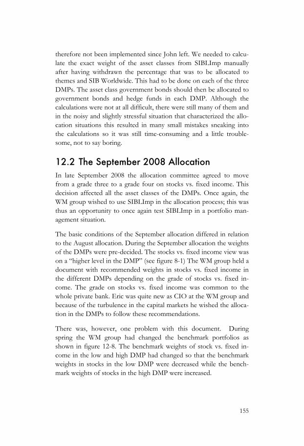
155

therefore not been implemented since John left. We needed to calcu-late the exact weight of the asset classes from SIBLImp manually after having withdrawn the percentage that was to be allocated to themes and SIB Worldwide. This had to be done on each of the three DMPs. The asset class government bonds should then be allocated to government bonds and hedge funds in each DMP. Although the calculations were not at all difficult, there were still many of them and in the noisy and slightly stressful situation that characterized the allo-cation situations this resulted in many small mistakes sneaking into the calculations so it was still time-consuming and a little trouble-some, not to say boring.

12.2 The September 2008 Allocation In late September 2008 the allocation committee agreed to move from a grade three to a grade four on stocks vs. fixed income. This decision affected all the asset classes of the DMPs. Once again, the WM group wished to use SIBLImp in the allocation process; this was thus an opportunity to once again test SIBLImp in a portfolio man-agement situation.

The basic conditions of the September allocation differed in relation to the August allocation. During the September allocation the weights of the DMPs were pre-decided. The stocks vs. fixed income view was on a “higher level in the DMP” (see figure 8-1) The WM group held a document with recommended weights in stocks vs. fixed income in the different DMPs depending on the grade of stocks vs. fixed in-come. The grade on stocks vs. fixed income was common to the whole private bank. Eric was quite new as CIO at the WM group and because of the turbulence in the capital markets he wished the alloca-tion in the DMPs to follow these recommendations.

There was, however, one problem with this document. During spring the WM group had changed the benchmark portfolios as shown in figure 12-8. The benchmark weights of stock vs. fixed in-come in the low and high DMP had changed so that the benchmark weights in stocks in the low DMP were decreased while the bench-mark weights of stocks in the high DMP were increased.

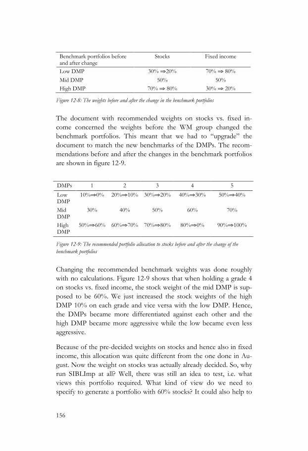
156

Figure 12-8: The weights before and after the change in the benchmark portfolios

The document with recommended weights on stocks vs. fixed in-come concerned the weights before the WM group changed the benchmark portfolios. This meant that we had to “upgrade” the document to match the new benchmarks of the DMPs. The recom-mendations before and after the changes in the benchmark portfolios are shown in figure 12-9.

Figure 12-9: The recommended portfolio allocation to stocks before and after the change of the benchmark portfolios

Changing the recommended benchmark weights was done roughly with no calculations. Figure 12-9 shows that when holding a grade 4 on stocks vs. fixed income, the stock weight of the mid DMP is sup-posed to be 60%. We just increased the stock weights of the high DMP 10% on each grade and vice versa with the low DMP. Hence, the DMPs became more differentiated against each other and the high DMP became more aggressive while the low became even less aggressive.

Because of the pre-decided weights on stocks and hence also in fixed income, this allocation was quite different from the one done in Au-gust. Now the weight on stocks was actually already decided. So, why run SIBLImp at all? Well, there was still an idea to test, i.e. what views this portfolio required. What kind of view do we need to specify to generate a portfolio with 60% stocks? It could also help to

Benchmark portfolios before and after change

Stocks Fixed income

Low DMP 30% ⇒20% 70% ⇒ 80%

Mid DMP 50% 50% High DMP 70% ⇒ 80% 30% ⇒ 20%

DMPs 1 2 3 4 5

Low DMP

10%⇒0% 20%⇒10% 30%⇒20% 40%⇒30% 50%⇒40%

Mid DMP

30% 40% 50% 60% 70%

High DMP

50%⇒60% 60%⇒70% 70%⇒80% 80%⇒0% 90%⇒100%

157

get Bill and Eric acquire a better understanding of the model and its behaviour. We used the model by testing it with different views and different levels-of-unconfidence. Bill was a little uncomfortable with this way of using the model. In some sense, it seemed he felt that we were somehow cheating by doing things backwards. My stand on this point was that, at this phase of the development of the SIBLImp, any kind of use, that could increase understanding on how the SIBLImp and the B-L model worked was reasonable.

12.3 Reflections on the Experiences from Using SIBLImp

Testing SIBLImp in real portfolio allocation generated insights con-cerning both the use of the B-L model in general and the use of SIB-LImp in particular. There are many issues that could be discussed and reflected upon when it comes to these tests. Five issues that seem interesting and important have been chosen. The two first are of a more organizational nature and concern the dependency on enthusi-asts in the project and the importance of working communication between the individuals within the organization. The use of reference portfolios when testing SIBLImp is then discussed, and mistakes and how these made ways for deeper understanding of both the B-L model and SIBLImp are presented. In conclusion, the use of proto-types is reflected upon.

The tests of SIBLImp were distinctly influenced by the fact that they were done without John present. This illustrates the dependency on individuals. Bill, who together with Eric was supposed to run SIB-LImp from now on, had been little involved in the development of SIBLImp and was not familiar with the B-L model. During the tests, however, Eric was not that much involved, so it was mainly Bill and I who engaged in the testing of SIBLImp. Since Bill had little know-ledge of the B-L model and SIBLImp it became my task to both ex-plain the B-L model and demonstrate SIBLImp while we performed the tests. If we had had more time, it would probably have been re-warding to have had at least one meeting before the tests were per-formed where we could have gone through the B-L model and SIB-LImp in peace and quiet. Because Bill did not have much knowledge about SIBLImp my role in the tests became more central than it

158

would probably have been if the tests had been performed together with John.

The fact that Eric and Bill intended to include a year of falling stock prices by choosing six instead of five years when in fact they would need seven years to include such a year, illustrates a shortcoming in communication. The length of historical data was decided by Eric and Bill very quickly while Eric was leaving for a meeting. I later con-fronted Eric with the fact that to include a year of falling stock mar-kets they would have needed to include seven years of historical data instead of six. Eric said that he believed that Bill and/or I would check to make sure that the time period chosen included a year of falling stock markets whether it was five, six or seven years of histori-cal data that needed to be included. At the time, I did not reflect on the time period chosen but believed that Bill and Eric had knowledge in these matters. This fact implies a problem in communication and roles between the three of us. The mistake with the length of histori-cal data, however, was not severe at this point since this was more of a trial run of B-L when reallocating the DMPs. The question is also how much effect one or two more years of historical added to the history when counting the covariance would have on the output port-folios.

One of the reasons for claiming that the mistake with the length of historical data was not particularly severe has to do with the fact that the WM group had a kind of reference portfolio in mind while per-forming the tests. Although not stated explicitly, the WM group had an idea of how they believed the holdings in the DMPs ought to look when the portfolios were reallocated. This became clear when Eric and Bill pointed out what they considered to be an unreasonably large weight of US stocks suggested by SIBLImp. When testing the B-L model and an application like SIBLImp, my belief has come to be that it is reasonable – if not a prerequisite – to have such a reference portfolio in mind. Without a reference portfolio it would have been difficult to evaluate whether SIBLImp output reasonable portfolios or not.

It seems to be of importance to investigate why the output portfolio does not match the reference portfolio and the user needs to question whether this is reasonable or not. As mentioned earlier, the weight of

159

US stocks in the portfolio output by SIBLImp did not match the reference portfolio Bill and Eric had in mind. They meant that there were far too much US stocks in the SIBLImp portfolio. Investigating this fact led to the insight that one of the views input to SIBLImp was actually incorrect. The view was expressed in relation to the port-folio held and not to the benchmark portfolio as specified by the B-L model. We might not have noticed this fact if they hadn’t had a refer-ence portfolio in mind. Hence, it might have taken much longer to realize the mistake made when expressing views without such a refer-ence portfolio. This issue probably accelerated the learning process of the B-L model and highlights (again!) the importance of understand-ing the B-L model to be able to use it rewardingly.

As these two allocations were the first times SIBLImp was used in real portfolio management, it was of extra importance to have such a reference portfolio to relate to. When the output portfolio from SIB-LImp differed substantially from the reference portfolio we examined why. When investigating these differences, it became clear that they were often due to the human factor, i.e. we had made mistakes when inputting data to SIBLImp. If there had not been a reference port-folio it would have been difficult to locate these errors. Bill wondered whether this was really a good way of using SIBLImp. My standpoint here was that as long as the program helps the decision making pro-cess it has fulfilled its purpose. It could in fact be so that SIBLImp will mostly be used in this way.

Working with the issues encountered during the tests was often time consuming and frustrating. However, the struggle to understand why SIBLImp behaved in certain ways and whether these behaviours were due to mistakes in or misunderstanding of the model or the program, generated deeper understanding of the B-L model and SIBLImp and their characteristics. As described earlier, in the August 2008 alloca-tion, after correcting the erroneous views, the SIBLImp still output too much US stocks in relation to the reference portfolio. Once again, we had to investigate the reasons for the divergence. This time it was not due to any mistake. As described earlier, the views input by the WM group concerned only the foreign stock portfolio and these were negative views on European and Japanese stocks and this needed to result in overweight in US stocks. There was no other asset

160

class to choose from. This behaviour was due both to the B-L model and how the model had been implemented in SIBLImp. What the WM group needed to do was to ask themselves whether this seemed reasonable and if they could work in this way. After some explan-ations and argumentation on my part, Bill and Eric seemed to find it quite a sensible way of working. This divergence from the output of SIBLImp and the reference portfolio had then resulted in a deeper understanding of both the B-L model and SIBLImp for all of us. This proves the importance of understanding the specific B-L implementa-tion one is working with.

During the allocations we experienced difficulties in translating view-expected-returns of the mid DMP to the low and high DMP. In the actual test situation it became complicated with much manual calcula-tion where small mistakes were easily made. There were other kinds of small mistakes that were made when using SIBLImp. Forming view-portfolios became a little complicated since we had to delete the preinstalled views because of their effect on the output portfolio. SIBLImp was however still a prototype and the plan was to handle these problems in future versions. Until this has been done I recom-mend the WM group to only use SIBLImp for the mid DMP since using this version of SIBLImp with the low and high DMP would be too complicated.

12.4 Conclusions: The B-L Model in Allocation This chapter exemplifies difficulties concerning the use of the B-L model that need to be addressed. The descriptions are far from the textbook or article descriptions of the model. They show the depend-ency on both individuals and the interaction between them. Mistakes of different magnitude and severity from just inputting wrong figures on the weights of the view portfolio on the view on Japanese vs. foreign stocks to the misunderstanding as to what portfolio (the port-folio held or the benchmark portfolio) views ought to be expressed.

Nevertheless, these two tests imply that the model can contribute to portfolio management in different ways and in ways not anticipated. The tool cannot only suggest portfolio weights. It can also increase the understanding of portfolio choice and be used to answer ques-tions of a “what if” nature, implying the views required considering a

161

specific portfolio. Last but not least, the B-L tool can act as a basis for dialogue on both views and portfolio weights. Later on, this dia-logue will surely also concern various types of risk measures.

162

13 Organizational Issues This chapter takes up organizational issues that have been of import-ance to the development of BLOld and SIBLImp and the use of these programs. It has already been shown that organizational chan-ges, organizational downsizing and individuals leaving the bank af-fected the development and use of SIBLImp. The programs are em-bedded in an organization and do not exist on their own.

First, the relation between the WM group and the rest of the organi-zation is taken up. This section concerns organisation on a corporate level. After that, two issues concerning the organisation of the project are discussed. The chapter ends with comments concerning the im-portance of enthusiasts in the project.

13.1 The WM group and SIB PB So far, relations between the WM group and the rest of SIB PB have not been mentioned. In fact, elements in the organization, outside the WM group, brought pressure to bear on the management of the DMP.

SIBLImp was supposed to be used by the WM group to manage the DMP. Relationship managers could recommend customers to hold the DMP (I here choose to use the singular since it was marketed

163

towards customers as a single product). Relationship managers can be described as SIB PB’s financial advisors. Their main task was to ad-vise customers on how to invest capital. They were mainly evaluated by the volume of their customer capital, how much new capital they generated and the revenues from their customer volume, often in relation to predefined estimated revenue. The relationship managers’ work mainly involved participating in meetings with new and existing clients to advise them on how to place their capital but also to analyse and pick products to recommend to clients.

The DMP had existed as a product since 2006. Ever since the launch, the WM group had been dependent on the relationship managers’ willingness to advise customers to hold this product. They had, how-ever, experienced difficulties in motivating the relationship managers to do so. An argument used by the relationship managers to explain why their customers did not invest in the DMP was that it was ex-pensive. They also had much of their customer capital invested in what they believed were good funds, i.e. funds that had performed well and were highly rated by rating institutes.

The problems that the WM group experienced in motivating relation-ship managers to advise customers to hold the DMP resulted in the WM group having to “sell” the DMP internally to the relationship managers. This activity meant that much time and energy were spent on preparing and holding internal presentations for the relationship managers where they described allocations within the DMP and mo-tivated why these where made.

In January 2009 complaints from relationship managers concerned the performance of the DMP. The DMP had then been over-weighted in stocks since October 2008, a not very good bet, given the financial crisis and the rapid fall of stock markets all over the world that characterized the autumn of 2008. Eric discussed a dilemma here. He admitted that overweighting stocks during this period was not the best decision, but also pointed out the difficulty of predicting the total crash of the financial market that occurred during this pe-riod. However, Eric said that he, during autumn 2008, had advised the relationship managers to lower the overall risk in their customer portfolios. He exemplified with the difference of a customer having the mid DMP instead of the high DMP. This implied a difference of

164

between approximately 50% and 70% stocks in the portfolio. The difference between the holdings of the mid DMP from the bench-mark weights of the same was around 3 percentage points, hence from 50% to around 53%. Eric felt a little annoyed by the many complaints about such an allocation when in his opinion the main problem was that customers had too risky portfolios overall.

This indicates that much of the holdings in a customer portfolio were already decided before the B-L model came into play. The most im-portant decision for a customer seems to be the decision concerning the weights of the strategic benchmark portfolio.

Reflections Since relationship managers were evaluated by the volume of their customers’ capital, how much new capital they generated and how much revenue their volume generated, it may seem a brilliant solution for them to recommend DMP to customers. Placing customer capital in the DMP could be seen as liberating time from managing port-folios to instead “selling” and therefore generating more capital to be managed. The WM group had, however, experienced great difficulties in convincing the relationship managers to recommend their custom-ers to invest in the DMP.

The relationship managers, in some sense, could however be seen as portfolio managers themselves. Towards their customers they were responsible for how the portfolios performed. One of the reasons why the problem of motivating them to recommend the DMP to customers may have been insufficient confidence in the management of the DMP. Since the DMP did not have a long history of perform-ance, confidence in the product had been closely related to the people managing it. When placing clients’ capital in the DMP the relation-ship managers in some sense handed over the responsibility of man-agement to the WM group. If the relationship managers did not have enough confidence in the management of the DMP, it is not difficult to understand their indisposition to recommend the DMP. Placing customer capital in the DMP could also appear to undermine their capabilities as financial advisors. Many of the relationship managers were earlier successful stockbrokers with high confidence in their

165

own investment skills. Also, their own investment skills might have been one of their main assets in their relationships with customers.

Although relatively resource-demanding with the internal selling ac-tivities between the WM group and the relationship managers, there seemed to be some advantages to this way of organising. It seems as if the relationship managers regarded the DMP as just another pos-sible asset to recommend and that their demands were as high on the DMP as on any other product that they would recommend to their customers. This ought to be good for the customers.

An effect of the dependency on the WM group on the relationship managers and their willingness to recommend customers to invest in the DMP had however resulted in the former trying to influence the DMP and its positions. Theme investments, as an asset class in the DMP, were the result of such influence. Another example was hedge funds. When the project began, John had not yet included hedge funds in the DMP but motivated the inclusion of that asset class with a desire to get more of the customer capital allocated to the DMP. A good way to achieve that was to take measures to increase the will-ingness of the relationship managers to advise customers to invest in the DMP.

As shown, the organizational context exercised influence on the use of the B-L model. Without the pressure from relationship managers it is not certain that theme investments and hedge funds would have been included into the DMP.

13.2 Project Issues Two issues concerning the communication within the project tem and the use of prototypes will be discussed in the following two sec-tions.

Understanding and communication A point of departure, stated in chapter 1.3, was that when using ap-plications like SIBLImp (hence implementing a theoretical financial model) it is important that users not only understand the model itself but also understand its specific implementation. When implementing financial models in computer applications, variables need to be esti-

166

mated. These estimations influence the behaviour of the application and hence it is of importance that users have a thorough understand-ing of both the model and the estimations made in order to imple-ment the model.

The case shows the importance of the consultant’s understanding the work situation of the principal. During the development of SIBLImp I believed that Tom’s and my understanding of the WM group’s work situation was thorough enough. In retrospect, however, this seems not to have been the case. This is elucidated by the fact that SIB-LImp(F) (working on fund level instead of on index level) was devel-oped. It seems that we had an insufficiently deep understanding of the WM group’s work to understand the problems associated with using this approach. Could this have been avoided?

If John had had a better understanding of the B-L model and the way it was implemented in SIBLImp it might have been possible for him to realize the problems in using SIBLImp(F) at an earlier stage and hence end the development of the application earlier. However, in this case it would have been quite unrealistic to demand of John that he have such detailed knowledge. My belief is that John’s previous knowledge concerning the B-L model was on a reasonable level when the project began.

Another way to avoid the detour to SIBLImp(F) and back to SIB-LImp might have been if Anders and I had had an even better and deeper knowledge of John’s and the WM group’s group. A very well working communication between John as taskmaster and us as con-sultants would also have helped our common understanding of how the WM group worked. If the communication between John and Tom and myself had worked even better, we might not have ended up spending time on developing SIBLImp(F).

Using prototypes BLImp was developed as a prototype or perhaps a pre-prototype while searching for a financial actor who wished to implement or use a B-L application. This pre-prototype was a prerequisite to get access to the case at SIB. Without BLImp it does not seem reasonable to believe that SIB would have “hired” Tom and me to develop SIB-LImp. In that sense, BLImp was essential to the project. In hindsight,

167

there seem to have been some problems involved in using this pre-prototype. BLImp came to work as a prototype for SIBLImp that was also a prototype version of a B-L tool. In a way BLImp steered the development of SIBLImp. BLImp prevented us in some sense from seeing other solutions to problems that occurred when develop-ing SIBLImp. One example is the problem with the different bench-mark portfolios in the three DMPs (chapter 11.1). However, the idea was to let John test BLImp and then evaluate what he liked and what he did not like. John never came to do this and important input to the development of SIBLImp was thus lost. If John and the WM group had been more involved in the development of SIBLImp the picture might have been a different one. Tom and I had developed BLImp in a way that we believed would be good and hence SIBLImp was implemented in similar ways but modified to the needs of the WM group.

In chapter 10, issues related to John’s expressed wish to understand the B-L model was discussed. In hindsight, there seem to be prob-lems associated with the way SIBLImp was introduced to John. Be-cause of my belief in the importance of understanding the specific tool one is working with, John’s desire to better understand the B-L model was much appreciated. His attitude however, inspired me to try to explain the B-L in detail to him. Afterwards the question is if the explanation might have been too detailed. It might have been difficult for John to see the wood for the trees. SIBLImp might have seemed difficult to use and hence prevented him from actually testing it.

However, the fact that the B-L model might have seemed more com-plicated than necessary might not only have had to do with my ex-planation of the same. The fact that SIBLImp was a prototype and developed as such, might have added to this impression. Tom and I did not want to spend too much time and money on development before we had received feedback from John and SIBLImp was there-fore associated with some problems, such as the fact that views needed to be expressed differently for all DMPs and that assets not included in SIBLImp generated portfolios did not include all assets held by the DMPs. The aim was to solve these issues later in interac-tion with John. However, since John had not tested BLImp or SIB-

168

LImp properly the shortcomings in SIBLImp may have given a mis-leading picture that the shortcomings in SIBLImp were indeed short-comings in the B-L model.

13.3 Importance of Enthusiasts Pete mainly developed BLOld. He had been the driving force behind the development and use of the program. When Pete left SIB, John already appreciated working with BLOld. No one at the WM group, however, was involved enough in the program to be able to use it or develop it. When Pete left SIB, BLOld therefore fizzled out. To han-dle the issue of not using BLOld, John contacted Tom and me and the development of SIBLImp began. At SIB John was the driving force behind the development of SIBLImp. When John left SIB, the development of SIBLImp was put on hold and the program was also used much less than it probably would have been if John had con-tinued working for SIB.

The course of events indicates the importance of individuals. Devel-oping these applications has taken resources from SIB both in con-sultancy costs and in man-hours. Having structures in the organiza-tion so that applications such as BLOld and SIBLImp are able to be used although the “originator” leaves the organization ought to be of importance.

13.4 Conclusions: Organisational Issues The above discussion shows that the organization both on the corpo-rate level as well as on project level had great impact on the SIBLImp and its use. It thereby emphasises the importance of taking such is-sues into account. This applies to individuals as well as their interac-tions and also to individual working teams and also the interaction between them.

169

14 Results and Comments on the Case

The aim of the third part has been to study the development and use of an application implementing the B-L model in an investment or-ganization, discuss these experiences and draw conclusions from them. Much of the results and contributions from the step is embed-ded in the above empirical descriptions and the reflections. This chapter lists the main results from step III. The case itself is then discussed and a short presentation given of events after the project ended in September 2008.

14.1 Results The presentation begins with results closely tied to the model itself, followed by results connected to the user of the model and finally results that more and more relate to the social and organizational situation. But, first comes a result connecting to these three nouns: model-user-situation.

Model-user-situation A general observation from the third step is that whether the use of the B-L model works well or not does not merely depend on the

170

model. The model is not isolated; it is embedded in a social and orga-nizational context in which a variety of variables outside the model exert influence on its use. The model should hence not be evaluated in isolation. The experiences imply that it is the model-user-situation combination that may prove profitable to a greater or lesser degree. Situation in this case involves both the specific organisation, time-period, individuals and business.

The features What does the experience of working with the case, and hence with the three different B-L implementations (BLImp, BLOld and SIB-LImp), imply to the key features of the B-L model?

The view feature appeared quite straightforward and intuitive when working with only one portfolio. Although the people at SIB were not particularly involved in the formation of view-portfolios, it was per-ceived as straightforward. However, SIB managed several portfolios and this generated the need to express different view-expected returns on views in the different portfolios, which was both intricate and unin-tuitive.

Weight-on-views has been surrounded with a considerable amount of theoretical mysticism (chapter 3). However, step I contributes a for-mula for this parameter and thereby highlights some of the concerns. In SIBLImp, weight-on-views was set to one, thereby excluding the parameter. The desire to exclude it was mainly due to the fact that several parameters interrelate within the B-L model and weight-on-views seemed to be the most reasonable to put on hold. Since weight-on-views was not used at SIB, there were few indications concerning the parameter from this case.

Levels-of-unconfidence, however, was surrounded by several difficulties. It was experienced as difficult to determine the approximate size of the parameter and difficult to understand how much to increase or de-crease it. Calculating and using market levels-of-unconfidence dealt with part of the problem by generating a neutral level-of-unconfidence as a starting point. However, it was still considered difficult to set its value. During the August and September tests, however, we began to develop a kind of heuristic on how to express this parameter. A doubled level of unconfidence came to represent a

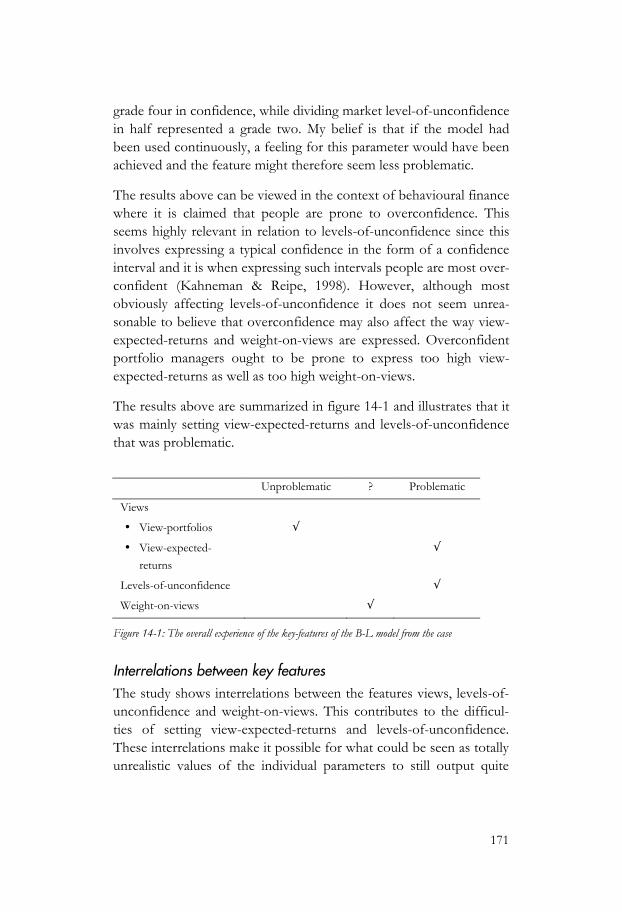
171

grade four in confidence, while dividing market level-of-unconfidence in half represented a grade two. My belief is that if the model had been used continuously, a feeling for this parameter would have been achieved and the feature might therefore seem less problematic.

The results above can be viewed in the context of behavioural finance where it is claimed that people are prone to overconfidence. This seems highly relevant in relation to levels-of-unconfidence since this involves expressing a typical confidence in the form of a confidence interval and it is when expressing such intervals people are most over-confident (Kahneman & Reipe, 1998). However, although most obviously affecting levels-of-unconfidence it does not seem unrea-sonable to believe that overconfidence may also affect the way view-expected-returns and weight-on-views are expressed. Overconfident portfolio managers ought to be prone to express too high view-expected-returns as well as too high weight-on-views.

The results above are summarized in figure 14-1 and illustrates that it was mainly setting view-expected-returns and levels-of-unconfidence that was problematic.

Unproblematic ? Problematic

Views

• View-portfolios √

• View-expected-returns

√

Levels-of-unconfidence √

Weight-on-views √

Figure 14-1: The overall experience of the key-features of the B-L model from the case

Interrelations between key features The study shows interrelations between the features views, levels-of-unconfidence and weight-on-views. This contributes to the difficul-ties of setting view-expected-returns and levels-of-unconfidence. These interrelations make it possible for what could be seen as totally unrealistic values of the individual parameters to still output quite

172

realistic portfolios. This may give rise to misunderstandings and prob-lems

Acceptance The study shows acceptance of the B-L model. A B-L inspired pro-gram (BLOld) was already in use at the bank when the project began and the people involved wished to continue working with such a program. During the development none of those involved wished to stop the model’s development or not use it.

Importance of individuals The study shows the importance, and also the difficulties, of getting users truly involved in the development of the B-L implementation. John did not properly test the program and the development process thereby missed out on important user feedback.31

The development of SIBLImp and BLOld was dependent on enthu-siasts. When the enthusiasts left the organisation, both development and use of the programs suffered.

Importance of understanding The study implies the importance of the user understanding the model. For example, as shown in chapter 12 the model seemed more intuitively correct to Eric and Bill when they understood that the model uses the benchmark portfolio as a point of reference and that views are supposed to be expressed in relation to that portfolio, not in relation to the portfolio’s current holding. This knowledge certainly increased their possibility to use the model profitably. However, it also indicates that there is a risk involved in “experts”, me in this case, trying to explain too many details that might not be needed at that specific time. The model and application might be perceived as more difficult than necessary.

31 Källström (1993, p. 219, 222) describes similar experiences concerning the development and introduction of decision support systems.

173

Using reference portfolios The study shows that having a reference portfolio in mind and a criti-cal attitude towards the model helped increase understanding. When the reference portfolio did not match the output portfolio and the question why was asked, our understanding of the tool increased (chapter 12.3).

Alternative use of the model The research indicates an alternative way of using the B-L model by beginning with the portfolio and then investigating what kind of views this portfolio would represent. A similar way of using the model was suggested by Black and Litterman (1990, p. 19). They refer to solving what views a certain portfolio would require as “implied views”.

Differences model – real world The study points at differences between the B-L model and the prac-tical situation at the bank. (1) SIB worked with several portfolios (low, mid and high risk) that held the same asset classes but different benchmark weights. The WM group had the same views for the three portfolios but since the benchmark weights differed between the DMPs this resulted in difficulties when trying to express the same views for all the DMPs. A similar situation was also shown to exist at the bank contacted before the SIB case. However, at that bank, each customer had an individual benchmark portfolio. (2) The WM group worked on two levels: they optimized and evaluated on asset class level but invested in specific funds. (3) The DMPs also held some assets for which they could not find good enough indices. These assets were therefore not included in the B-L model. These are ex-amples of differences between the situation implicit in the B-L model and the situation that came about in the case.

Influence of social situation and organisational contexts The study emphasizes that social and organizational contexts had a distinctive impact on the development and use of SIBLImp. (1) The organizational situation led to the WM group becoming very depend-ent on the relationship managers since they were the ones able to advise customers to hold the product. (2) Communication within the

174

project seems not to have been perfect. Better communication might for instance have led to the development of the SIBLImp on fund level being avoided. (3) Organizational restructuring and the financial crisis of 2008 affected the use and development of SIBLImp.32

The above results are different in character and imply the width of the results in this kind of qualitative case research. While some results are related to the model itself, others deal with the individuals and the users of the implemented version of the B-L model. The third type of results presented are of a more organizational nature and imply that the social situation and organizational context are crucial to the B-L model and its use.

14.2 Comments on the Case The research has focused on one case and it is therefore not possible to generalise in any statistical sense. It is relevant to consider the rep-resentativeness of features of the case.

It seems that the way SIB worked was not atypical. Working with several benchmark portfolios where the risk of the portfolios is de-termined by the weights of the benchmark seems to be quite com-mon. According to Eric, who has been working with private banking for 10 years and has worked at three other private banks, this is a common way of working. Also, the bank that was contacted before SIB proved to work in a similar way. At that bank, each customer had his or her own benchmark portfolio, so the number of benchmark portfolios could be the same as the number of customers. Allocating on asset class level but still investing in specific funds seems not un-usual either, at least not in the private banking sector, according to Eric.

However, the time period when this case was performed was not representative. It was actually very unusual since it ended in the fi-nancial crisis of 2008, one of the most severe global financial crises of modern times.

32 Both (2) and (3) resemble experiences from Källström (1993, p. 219, 222)

175

Within this case, there are in some sense two subcases. The “other bank” represents another example of a bank working with several portfolios with different benchmarks for which they wish to express the same views. The BLOld represents another program implement-ing the B-L model and although BLOld and SIBLImp are not inde-pendent, at least they represent two different ways of implementing the B-L model in the same portfolio management organisation.

14.3 Case Epilogue The performance of the DMPs has hitherto not been commented upon. One reason for this is that this study does not evaluate how SIBLImp or the B-L model performs. Output portfolios of the B-L model are very much dependent on the input to the model and thus the views expressed by the user. If the B-L model generates poorly performing portfolios because the views input to it are weak, the blame should not fall on the model but on the views: garbage in gar-bage out. This was commented upon by Litterman himself during a lecture at Goldman Sachs (Nordic Summit 2007-09-27) where he verified the notion by claiming that there is no way to actually test the B-L model in this way since the output portfolios always depend on input data.

It could however, in retrospect, be of interest to briefly comment on the outcome. In September 2008, the allocation group increased the grade on the view on stocks vs. fixed income from a grade three to a grade four. This was just before the 2008 financial crisis and naturally affected the performance of the DMPs negatively. The allocation group could have agreed to revert to a grade three, or possibly even lower, for the view on stocks vs. fixed income at their October meet-ing. They chose, however, to stick to the grade from September. They could not foresee the depth of the crisis and chose not to lower the grade because of the risk of decreasing the amount of stock by the time stock markets began to recover. The fact that the grade on stocks vs. fixed income was kept led to it being kept for a very long time and it was not changed until November 2009 when the grade on stocks vs. fixed income was lowered from a grade four to a grade three.

176

The fact that we were so early, too early, to raise the grade on stocks vs. fixed income meant that we had no reason to change this grade for over a year, notwithstanding the financial crisis.

(Eric, 2010-10-15)

The DMPs thus did not perform well during autumn 2008. 2009, however, was the best year in the not so long history of the DMP.

After this project had ended, the SIBLImp needed improvement to work smoothly. I recommended SIB to only use SIBLImp to allocate the mid DMP until further development had been carried out. So far there has been no more development of SIBLImp, but Eric still claims that they have use of the tool when allocating. However, they still have reference portfolios that they wish to invest in when using the B-L model but test what views that are required to make SIB-LImp output such a portfolio.

When talking to Eric in October 2010, new major organizational changes have begun at SIB. Eric, however, has expressed a desire to continue the development of SIBLImp and maintains that that has always been the idea but since autumn 2008 the situation at SIB has been very volatile and he has not been able to find the time and money to engage in the activity of continuing the development of SIBLImp. It does not seem unreasonable to assume that many devel-opment projects within the banking industry have experienced similar pauses because of the financial crisis and its aftermath.

2010-11-15 Pete, John and Eric, answered questions concerning the B-L model via email. The questions concerned the added value of using the model and the advantages and disadvantages of the same.

Pete stressed the possibility to create an equilibrium portfolio that can be tilted in the direction of views as an advantage. John and Eric focused more on how using the model gives structure to the problem and the decision process. Eric found that expressing view-expected-returns and levels-of-unconfidence is rewarding. John found the ag-gregated conjunctions within the model to be an advantage. He stressed that using the model gives guidance to more sober decisions. It became clear that neither Pete, John nor Eric considered the use of the B-L model to “take” the allocation decision but that it can be used to simulate (forward and backward) and that these simulations

177

can be rewarding input to discussions and to the decision process. The fact that it is an academically accepted model was seen as an advantage as well as the fact that it is developed within Goldman Sachs. A disadvantage is that you cannot include theme investments and that market returns are theoretical and difficult to assimilate and understand. Expressing confidence as standard deviations was also seen as a disadvantage especially for those not that mathematically acquainted.

179

Ending

181

15 Concluding Discussion The first part of this chapter summarizes the results from the thesis and divides them into results about the model, the indi-vidual user and the situation. Two strong impressions from working with the research are then presented. The chapter concludes with ideas about how to continue development of the B-L model.

15.1 Summary of Results The development of the B-L model has been regarded as a process (chapter 1.3). The question is what contributions the three steps make to the on-going development process. The title of the thesis indicates that the focus has been on the B-L model. Although social and orga-nizational contexts are observed and discussed, the focus has none-theless been on the model itself and its use. One reason for this is that there were theoretical knowledge gaps that needed to be filled before qualitative case research seemed appropriate. Working with both the theoretical parts of the model and the case has generated results and contributions of different kinds.

Since the first two steps of the thesis are of a more theoretical nature than the third, it is easy to assume that these first two studies contri-

182

bute to theory while the third contributes to practice. This, however, would assume that case study research or action science could not contribute to theory and that theory development could not contri-bute to practice. Instead, all the studies contribute to the develop-ment of the B-L model and have both theoretical and practical impli-cations. Results from the three steps are summarized below from a model-user-situation perspective (figure 15-1).

Model User Situation A detailed derivation of the B-L model from a sampling theory ap-proach. (I)

Interest in and acceptance of the B-L model. (III)

Distinctive impact of social and organizational contexts: (III)

An interpretable formula for the parameter weight-on-views. (I)

Importance of getting users involved in devel-opment. (III)

− People outside the user group exerted influence on the use of the B-L model. (III)

A new interpretation of levels-of-unconfidence. (I)

Dependency on enthusi-asts within the organisa-tion. (III)

− Reorganizations and 2008 crisis affected the use and devel-opment of the B-L model. (III)

Support for reference based portfolio models such as the B-L model. (II)

Importance of users understanding the B-L model. (III)

Differences between the B-L model and the practical situation: (III)

Difficulties in assessing size of levels-of-unconfidence. (III)

Alternative ways of using the B-L model. (III)

− several portfolios with the same asset classes but different benchmark weights. (III)

Market levels-of-unconfidence seemed as a usable point of refer-ence. (III)

Overconfidence problem-atic when estimating levels-of-unconfidence and weight-on-views. (II)

− two levels, optimiz-ing on asset class level but investing in specific funds. (III)

Confusing interrelations between views, levels-of-unconfidence and weight-on-views (III)

− some asset classes couldn’t be included in the B-L model. (III)

Figure 15-1: Results from the three steps summarized from the model-user-situation perspective, brackets indicate from which step certain results come

183

15.2 Strong Impressions Working with the project has given two experience-based impres-sions of a more holistic nature: the great distance between theory and practice and the importance of understanding.

Theory and practice A strong and growing impression from the research has been the great distance between theory and practice. The plan was from the beginning to perform a case study on the B-L model. However, more than half of the research carried out has concerned model issues that needed to be investigated and developed before a case study seemed appropriate. Theoretical research, in the form of a derivation of the B-L model from a sampling theory approach and drawing implica-tions from research within behavioural finance, pushed the develop-ment process to the point where it seemed profitable to study the model in practice. The time that elapsed and the amount of work involved to arrive at the point where an implemented version of the B-L model could be tested, were both also much greater than antici-pated. And although the research resulted in testing the implemented version of the B-L model, it did not come further than two introduc-tory tests of the model – far from continuous use.

The distance between theory and practice, in this case, should how-ever be considered in light of the origin of the B-L model. The B-L model is developed within modern finance, which, in turn, is based on economics. These subjects build on assumptions about rational decision-makers i.e. homo economicus and efficient financial mar-kets33.

When trying to take the actual behaviour of individuals into account, it was natural to turn to behavioural finance. Behavioural finance has proved that people systematically deviate from acting rationally and shown the ways in which this behaviour departs from the behaviour of homo economicus. The field thereby provides interesting know-ledge about how individuals behave when taking financial decisions

33 Compare with the discussion about “inefficient markets” in for instance Shleifer (2000).

184

and of how this affects the financial markets. The subject focuses on the individual investor and does not to any great extent take the social and organisational situation within which individuals act into account (see chapter 6.3).

In step III the case concerns the B-L model implemented in an orga-nization. Organizations add further dimensions of complexity be-cause the organizational context and also the cultural and social ditto exert influence on the use of the B-L model. However, there is no well-established financial research field that takes such an approach. Nevertheless, different streams of such research, referred to in this thesis as alternative finance (briefly discussed in chapter 7.2 and pre-sented in more detail in appendix 6) endeavour to extend financial research with knowledge about the cultural, social and organisational contexts surrounding financial activities. Several researchers within these streams maintain that financial research needs to be broadened to also include the realities that are studied, i.e. research needs to interact with those organisations and individuals engaging in the ac-tivities the research concern.

It does not therefore seem particularly surprising that it took much work to arrive at a position where case study research seemed appro-priate. The distance between theory and practice in this case depends on the distance between modern finance and research taking social and organisational contexts into account. The research in this thesis thereby strengthens the above arguments concerning the need for broadened financial research. Not least the need for research taking in organizational theory that has the opportunity to further increase awareness and understanding of cultural, social and organizational impact on the use of the BL model.

Understanding and distanced approach A point of departure of the thesis has been the importance of users understanding the tool they are working with. This point of view has been strengthened by the research (see chapter 14.1). Also, results from the research seem to have the possibility to increase under-standing of the B-L model.

It is easily assumed that the endeavour with a B-L tool would be to develop it to the point where users express input, run the B-L model

185

and then more or less directly invest in the portfolios generated by the program. There would, however, be risks involved in working with such a tool. Svahn (2009, p. 249) explains that the better the model the greater the risk that one attribute it too broad use or even mistake it for reality. Göranzon (1990, p. 57) discusses how comput-erization and the use of such applications have a tendency to reduce know-how. According to Göranzon, the program can break the im-portant link between the calculation and assessment (Göranzon, 1990, p. 67). Derman & Wilmot (2009) make comment in the same direction when claiming that:

You must start with models and then overlay them with com-mon sense and experience.

(Derman & Wilmott, 2009, p. 2)

Cederwall, quoted in Swahn (2009 p. 270), expresses the risks of be-coming dependent on too advanced modelling without understanding it and claims that one has to understand the physics of the model and be self-critical. Although Cederwall’s field is civil engineering, his argumentation appears to relate well to other types of models and their use.

If users understand the model as well as the specific implementation they are working with, this enables a distanced attitude towards the B-L tool and its output.

15.3 Moving On… How to continue the process of developing the B-L model? One, quite dramatic, assertion could be to advise the abandonment of the whole B-L idea. The results from the study do not however point in that direction. The individuals using it seemed to appreciate its fea-tures, find the output intuitive and appealing, and wish to continue working with it. However, more research and development are needed.

As discussed, the studies have shown that conditions outside the B-L model affect its use. Although individuals are important, social and organizational issues also influence the model. Use of the B-L model is three-dimensional. It depends on the model-user-situation.

186

Three suggestions for how two move the development process for-ward are presented below. The suggestions go from focusing on the model to focusing the user and then the situation.

Sub-models Results from the thesis indicate that banks not seldom manage sev-eral portfolios with different benchmarks for which they nonetheless want to express the same views. It seems as if it would be possible to develop a sort of sub-B-L-model that could be used at banks with similar ways of working. This can be compared with a subclass in object-oriented programming. The B-L model could be considered a class, the situational B-L model a sub-class and the implemented models such as for example the programs discussed in this thesis, BLOld, BLImp and SIBLImp, would be instances of the sub-class. More case research on the B-L model could probably find similar kinds of issues where the model does not match the situation for which other situational B-L models or sub-B-L-models could be de-veloped.

Overconfidence As indicated by step II there are problems regarding overconfidence related mainly to the use of levels-of-unconfidence but also to the use of weight-on-views. One of the most well established research results within behavioural finance is that individuals are prone to state too small confidence intervals. And, confidence intervals are exactly what are supposed to be estimated when expressing levels-of-unconfidence. However, the B-L model provides an interesting possibility to examine the overconfidence of the user. It would be possible to save the confidence intervals and then evaluate how often the actual return is within these intervals. Are users of the B-L model overconfident and if so how much? Does overconfidence increase after times of good performance? Will portfolio managers use this measure and if so in what way? Can they calibrate their confidence?

Praxis perspective Qualitative research on more mature use of the B-L model seems urgent on the basis of insights gained from step III. How are the key features expressed? How is the model used? Does the same person set all the parameters or might different individuals or groups set

187

levels-of-unconfidence contra weight-on-views? Is the model used in some totally unforeseeable way?

The research could draw upon the perspective on praxis34. Svahn (2009, p. 55) sees this perspective as an important complement to psychological and organizational perspectives. Such research could then contribute by extending the model-user-situation perspectives with a perspective on praxis.

Finally, as has been said many times in this thesis, it seems important to take cultural, social and organizational contexts into account.

34 See Johannessen (1999) for a further presentation of the concept praxis.

189

Literature

Abarbanell, J., Bernard V., (1992) Tests of analysts’ overreaction/ underreaction to earnings information as an explanation for an-omalous stock price behaviour, Journal of Finance, Vol. 47, No. 3, pp. 1181-1207.

Alvesson, M., & Sköldberg, K., (2008) Tolkning och Reflektion: veen-skapsfilosofi och kvalitativ metod, Lund: Studentlitteratur.

Alvesson, M., & Sköldberg, K., (2009). Reflexive methodology: New vistas for qualitative research. London: Sage.

Barber, B. M. & Odean T., (1998) Boys will be Boys: Gender, Over-confidence, and Common Stock Investment, Working paper (November 1998) http://ssrn.com/abstract=139415.

Barber. B. M. & Odean T., (1999) The Courage of Misguided Convic-tions: The Trading Behaviour of Individual Investors, Financial Analyst Journal, Vol. 55, No. 6, pp. 41-55.

Barberis, N. & Thaler R., (2003) A Survey of Behavioural Finance, in G. Constantinides, M. Harris & R. Stulz, (eds.), Handbook of the Economics of Finance, Amsterdam: Elsevier Science B.V.

190

Barnett, Vic, (1999) Comparative Statistical Inference, 3 ed., New York: Wiley.

Bentham, J., (1789) An Introduction to the Principles of Morals and Legisla-tion, New York: Oxford University Press 2005.

Beunza, B. & Stark D., (2004), Tools of the Trade: The Socio-Technology of arbitrage in a Wall-Street Trading Room, Industrial and Corporate Change, Vo. 13, No. 2, pp. 369-400.

Bevan, A., & Winkelmann K., (1998) Using the Black-Litterman Global Asset Allocation Model: Three Years of Practical Experi-ence, Fixed Income Research, Goldman Sachs & Co, wwww.hss.caltech.edu/media/from-carthage/filer/263.pdf.

Black, F., (1986) Noise, Journal of Finance, 41, July, pp. 529 – 543.

Black F., (1989) Universal Hedging: How to Optimize Currency Risk and Reward in International Equity Portfolios, Financial Analyst Journal July/August 1989, pp. 16-22.

Black, F. & Litterman R., (1990) Asset Allocation: Combining Inves-tors Views with Market Equilibrium, Fixed Income Research., Gold-man, Sachs (September 1990).

Black, F. & Litterman R., (1992) Global Portfolio Optimization, Fi-nancial Analysts Journal, Vol. 48, No. 5, pp. 28-43.

Blomberg, J., (2005) Finansmarknadens aktörer, Malmö: Liber.

Bondio, J., (2003) New Assumptions for a New Economics, Post-Autistic Eeconomics Review, Issue 19, article 4.

Borkin, Danielson, Ekenberg & Larsson, (2009) Bortom business intelli-gence, Stockholm: Sine Metu Productions.

Camerer, C.F. & Loewenstein G., (2004) Behavioural economics: Past, present, future, in C.F Camerer, G. Loewenstein. & M. Rabin (eds.) Advances in Behavioural Economics, New York: Princeton University Press.

191

Canner, N., Mankiw, N. G. & Weil, D. N., (1997) An Asset Alloca-tion Puzzle, The American Economic Review, Vol. 87, No. 1, pp. 181-191.

Christodoulakis, G.A. & Cass, J.C., (2002) Bayesian Optimal Port-folio Selection: the B-L Approach, Notes for Quantitative Asset Pric-ing MSc Mathematical Trading and Finance. http://scholar.google.com/url?sa=U&q=http://www.staff.city.ac.uk/~gchrist/Teaching/QAP/optimalportfoliobl.pdf.

Corley, K., (2004) Defined by our strategy or culture? Hierarchical differences in perceptions of organizational identity and change, Human Relations, Vol. 57, No. 9, pp. 1145–1177.

Eric, K., Hirshleifer, D. & Subrahmanyam, A., (1997) A theory of overconfidence, self-attribution, and security market under- and over-reactions, Unpublished working paper. University of Michigan.

Dawes, R. M., Faust, D., & Meehl, P. E., (1989) Clinical versus actu-arial judgment. Science, Vol. 243. No. 4899, pp. 1668 – 1674.

DeBondt, W., (1993) Betting on trends: intuitive forecasts of financial risk and return, International Journal of Forecasting Vol. 9, Issue 3, pp. 355-371.

DeBondt, W., & Thaler, R., (1985) Does the Stock Market Overre-act?, Journal of Finance, Vol. 40, No. 3, pp. 793-805.

de Goede, M., (2005) Resocialising and Repoliticising Financial Mar-kets: Contours of Social Studies of Finance, Economic Sociology: European Electronic Newsletter, no. 3 (July 2005): http://econsoc.mpifg.de/archive/esjuly05.pdf, pp. 19-28.

Derman, E., (2004) My Life as a Quant: Reflections on Physics and Finance, Wiley, New York.

Derman, E. & Wilmott, P., (2009) The financial modelers’ manifesto, November 2010: http://www.jnazlvxtp.gbkr.com/pdf/090107_fmm.pdf.

192

Devenow, A. & Welch I., (1996) Rational herding in financial eco-nomics, European Economic Review, Vol. 40, Issues 3-5, 603-615.

Edwards, W. (1968) Conservatism in human information processing, in B. Kleinmuntz, eds. Formal Representation of Human Judgment, Wiley, New York, pp. 17-52.

Elton, E.J. & Gruber, M.J., (1997) Modern portfolio theory, 1950 to date, Journal of Banking & Finance Vol. 21, Issues 11-12, pp. 1743-1759.

Falk, R. & Konold, C., (1997) Making sense of randomness: Implicit encoding as a bias for judgment, Psychological Review, Vol.104, No. 2. pp. 301-31.

Fama, E. F., (1970) Efficient Capital Markets: A Review of Theory and Empirical Work, Journal of Finance. Vol. 25, No. 2, pp. 383-417.

Fisher, K.L. & Statman, M., (1997) The Mean-Variance-Optimization Puzzle: Security Portfolios and Food Portfolios, Financial Analysts Journal, Vo. 53, No. 4, pp. 41-50.

Forslund, D., (2008), Hit med pengarna, , Falun: ScandBook.

Frankfurter, G. M., (1994) The end of modern finance International Review of Financial Analysis Vol. 3, Issue 3, 1994, pp. 7-9.

Frankfurter, G. M., Haugen, B., McGoun, E., Salandro, D. & Phillips, H. (1997) Pushing the Epsilon to the Abyss Post Modern Fi-nance, International Review of Financial Analysis, Vol. 6, No. 2: pp. 133-177.

Frankfurter, G. M. & McGoun, E. G., (2002) Resistance is futile: the assimilation of behavioural finance, Journal of Economic Behaviour & Organization, Elsevier, Vol. 48, No. 4, pp. 375-389.

Friedman, M., (1953) Essays in Positive Economics. Chicago: University of Chicago Press.

193

Fullbrook, E., (2002) A Brief History of the Post-Autistic Economics Movement, http://www.paecon.net/PAEhistory02.htm; 2005-09-22.

Fullbrook, Edward, (2005), Competitive and Non-Competitive Nar-ratives, Working paper, http://www.btinternet.com/~pae_news/Fullbrooknarratives.htm; 2005-09-22.

Fung W. & Hsieh, D.A., (2002) Hedge-fund benchmarks: Informa-tion content and biases, Financial Analysts Journal, Vol. 58, No. 4, pp. 22-34.

Gervais, S. & Odean, T., (2001) Learning to be overconfident, Review of Financial Studies , Vol. 14, No. 1, pp. 1-27.

Giacometti, R., Bertocchi, M. I., Rachev, S. T. & Fabozzi F. J., (2007) Stable Distributions in the Black-Litterman Approach to Asset Al-location, Quantiative Finance, Vol. 7, No. 4, pp. 424-433.

Gilovich, T., Griffin, D. & Kahneman, D., (2002) Heuristics and Biases: The Psychology of Intuitive Judgement, New York: Cambridge Univer-sity Press.

Gilovich, T., Vallone, R. & Tversky, A., (1985) The hot hand in basketball: On the misperception of random sequences, Cognitive Psychology, Vol. 17, Issue 3, pp 295-314.

Griffin, D., W. & Tversky, A., (1992) The Weighting of Evidence and the Determinants of Confidence, Cognitive Psychology Vol. 24, Issue 3, pp. 411-435.

Göranzon, Bo (1990), Det praktiska intellektet, Uddevalla: MediaPrint.

Hammarén, Maria (1995) Skrivande – en metod för reflektion, Stockholm: Utbildningsförlaget Brevskolan.

Hartman, R. S., Doane, M. J. & Woo, C.-K., (1990) Status quo bias in the measurement of value of service, Resources and Energy, Vol. 12, Issue 2, pp. 197-214.

194

He, G. & Litterman, R., (1999) The Intuition Behind Black-Litterman Model Portfolios, Technical report, Goldman Sachs Invest-ment Management Series, Fixed Income Research, December 1999.

Idzorek, T., (2004) A Step-by-Step Guide to the Black-Litterman Model, Working paper. http://www.economia.unimore.it/pattarin_francesco/didattica/papers/idzorek_2004.pdf.

Johannessen, K.,S., (1999) Praxis och tyst kunnande, Trydells tryckeri.

Jönsson S. & Lukka, K., (2005) Doing interventionist research in management accounting, GRI-rapport, nr 2005:6.

Jönsson S. & Lukka, K., (2006) There and Back Again: Doing Inter-ventionst Research in Managemnt Accounting, in C. S.,Chapman, A. G. Hopwood & M. D. Shields (eds) Handbook of Management Ac-counting Research, Elsiver pp. 373-398.

Kahneman, D., Knetsch, J.L. & Thaler, R.H., (1991) Anomalies: The endowment effect, loss aversion, and status quo bias, in D. Kahneman & A. Tversky, (2000) Choices, Value and Frames, pp. 159-170.

Kahneman, D., & Riepe, M., (1998) Aspects of investor psychology, The Journal of Portfolio Management, Vol. 24, No. 4, pp. 52-65.

Kahneman, D., Slovic, P. & Tversky, A., (1982) Judgment under uncer-tainty: Heuristics and biases. New York: Cambridge University Press.

Kahneman, D., & Tversky, A., (1973) On the psychology of predic-tion, Psychological Review, Vol. 80, No. 4, pp. 237-25l.

Kahneman, D. & A. Tversky, (1979) “Prospect theory: An analysis of decisions under risk.” Econometrica, Vol. 47, No. 2, pp. 313-327.

Kahneman, D., & Tversky, A., (2002) Choices, values and frames, New York: Cambridge University Press.

195

Kanter, A., (2004) The Bayesian Approach to Optimal Asset Alloca-tion Working paper, 2010-11-12: http://web.wits.ac.za/Academic/Science/CAM/Mfinance/Research/

Keasey, K. & Hudson, R., (2007) A house without windows, Critical Perspectives on Accounting, Vol. 18, Issue 8, pp. 932-951.

Klayman, J., Soll, J.B. & Gonzalez-Vallejo, C. and Barlas, S., (1999) Overconfidence: It depends on how, what and whom you ask, Or-ganizational Behaviour and Human Decision Processes, Vol. 79, Issue 3, pp. 216-247.

Knetsch, J. L., (1989) The Endowment Effect and Evidence of Non-reversible Indifference Curves, in D. Kahneman & A. Tversky (2000) Choices, Value and Frames. New York: Cambridge University Press, pp. 171-179

Knetsch, J. L. & J. A. Sinden, (1984) Willingness to Pay and Compen-sation demanded: Experimental Evidence of an Unexpected Dis-parity in Measures of Value, Quarterly Journal of Economics 99(August): 507-521.

Källström, A., (1993) Beslutsstöd – Två fallstudier om utveckling av stöd för ekonomiskt beslutsfattande, Göteborg: Vasastadens bokbinderi.

Laibson, D. & Zeckhauser, R., (1998) Amos Tversky and the Ascent of Behavioural Economics, Journal of Risk and Uncertainty, Vol. 16, pp. 7–47.

Lewin, K., (1946) Action research and minority problems, Journal of Social Issues, Vol. 2, No. 4, pp. 34-46.

Lincoln Y.S. & Guba, E. G. (1985) Naturalistic inquiry, Newbury park: Sage.

Litterman, B., (2003a) Introduction: Why an equilibrium approach? in Litterman et. al. Modern Investment Management- an equilibrium ap-proach, New Jersey: Wiley, pp. 3-8.

196

Litterman, B., (2003b) Global equilibrium expected returns, in Lit-terman et. al. Modern investment management- an equilibrium approach, New Jersey: Wiley, pp. 55-75.

Litterman, B., (2003c) Beyond equilibirium, the Black-Litterman Ap-proach, in Litterman et. al., Modern investment management- an equilib-rium approach, New Jersey: Wiley pp. 76-88.

Litterman et. al., (2003) Modern investment management- an equilibrium approach, New Jersey: Wiley.

Lord, C.G.,. Ross, L. & Lepper, M.R., (1979) Biased assimilation and attitude polarization: the effects of prior theories on subsequently considered evidence, Journal of Personality and Social Psychology, Vol. 37. pp. 2098-2109.

MacKenzie, D., (2010) About social studies of finance, www.sociology.edu.ac.uk/finance/about.htm, 2010-09-08.

MacKenzie, D, (2005a) Opening the black boxes of global finance, Review of International Political Economy, Vol. 12, No. 4, pp. 555 – 576.

MacKenzie, D. (2005b) How a superportfolio emerges: Long-term capital management and the sociology of arbitrag,e in K. Knorr Cetina, & A. Preda, (eds.), The Sociology of Financial Markets. New York: Oxford University Press.

Markowitz, H., (1952) Portfolio Selection, The Journal of Finance, Vol. 7, No. 1, pp. 77-91.

Markowitz, H., (1991) Portfolio Selection, Massachusetts: Blackwell Pub-lishers Inc.

Massa, M. and Simonov, A., (2003) Behavioural biases and portfolio choice”, Working Paper, Stockholm School of Economics.

McCloskey, D. N., (1998) The rhetoric of economics, 2nd ed., Madison: The university of Wisconsin press.

197

Meehl, P.E., (1954) Clinical versus Statistical Prediction: A theoretical analy-sis and a review of the evidence. Minneapolis: University of Minnesota Press.

Merriam, S. B., (1998) Fallstudien som forskningsmetod, Lund: Studentlit-teratur.

Michaud, R. O., (1989) The Markowitz Optimization Enigma: Is ‘Optimized’ Optimal?, Financial Analyst Journal, Vol. 45, No. 1, pp. 31-42.

Miller, D.T. & Taylor, B.R. ,(1995) Counterfactual thought, regret, and superstition: How to avoid kicking yourself, in T. Gilovich, D. Griffin & D. Kahneman, Heuristics and Biases: The Psychology of Intui-tive Judgement, New York:Oxford University Press, pp. 367-378.

Odean, T., (1998a) Are Investors Reluctant To Realize Their Losses?, Journal of Finance, Vol. 53, No. 5, pp. 1775-1798.

Odean, T., (1998b) Volume, volatility, price, and profit when all trad-ers are above average, Journal of Finance Vol. 53, No. 6 pp. 1887-1934.

Pafka, S. & Kondor, I., (2002) Noisy covariance matrices and port-folio optimization II, Physica A: Statistical mechanics and its ap-plications, Vol. 319, pp. 487-494.

Rabin, M., (1996) Psychology and economics, Journal of Economic Lit-erature, Vol. 36, No. 1, pp. 11-46.

Samuelson, W. & Zeckhauser, R., (1988) Status Quo Bias in Decision Making, Journal of Risk and Uncertainty, Vol. 1, No. 1, pp. 7-59.

Satchell, S., & Scowcroft, A., (2000) A Demystification of the Black Litterman model: Managing Quantitative and Traditional Portfolio Construction, Journal of Asset Management, Vol. 1, No. 2, pp.138-150.

Schachter, S., Hood, D.C, Andreassen, P.B. & Gerin, W., (1986) Aggregate variables in psychology and economics: Dependence

198

and the stock market, in B. Gilad and S. Kaish (eds), Handbook of Behavioural Economics, Vol. B, Greenwich: JAI Press, pp. 237-272.

Scharfstein, D. & Stein, J. (1990) Herd behaviour and investment, American Economic Review, Vol. 80, No. 3, pp. 465-479.

Schein, E. H., (2001) Clinical Inquiry/Research, in P. Reason & H. Bradbury (eds), Handbook of Action Research, California: Sage, pp. 228-237.

Shah, S. K. & Corley, K. G. (2006), Building Better Theory by Bridg-ing the Quantitative–Qualitative Divide, Journal of Management Stud-ies, Vol. 43, pp. 1821–1835.

Shani, A. B., Tom, A. & Willson, C., (2004) Collaborative Research - Alternative Roadmap, in N. Adler, A. B. Shani & A. Styhre (eds), Collaborative Research in organizations: foundations for learning, change, and Theoretical Development, London: Sage Publications, pp. 83-100.

Sharpe, W. F., (1967) Portfolio Analysis, The Journal of Financal and Quantitative Analysis, Vol. 2. No. 2, pp. 76-84.

Shefrin, H. & Statman, M., (1985) The Disposition to Sell Winners Too Early and Ride Losers Too Long: Theory and Evidence, Jour-nal of Finance, Vol. 40, No. 3, pp. 777-790.

Shefrin, H. & Statman, M., (2000) Behavioural Portfolio Theory, Journal of Financial and Quantitative Analysis, Vol. 35, No. 2, pp. 127–151.

Shefrin, H., (2002) Beyond Greed and Fear, New York: Oxford univer-sity press.

Shiller, R. J., (1998) Human Behaviour and the Efficiency of the Fi-nancial System, NBER Working Papers 6375, National Bureau of Economic Research, Inc.

Shleifer, A., (2000) Inefficient markets : an introduction to behavioural finance, New York: Oxford Univ. Press.

199

Smith, A., (1759) Part VI: Of the Character of Virtue Consisting of Three Sections, The Theory of Moral Sentiment, http://www.marxists.org/reference/archive/smith-adam/works/moral/part06/part6a.htm

Stake, R. E., (1978) The Case Study Method in Social Inquiry, Educational Researcher, Vol. 7, No. 2, pp. 5-8.

Statman, M., & Thorley, S., (2001) Investor Overconfidence and Trading Volume, Working Paper, Santa Clara University.

Stracca, L., (2002) Behavioural finance and aggregate market behav-iour: Where do we stand?, Working Paper, European Central Bank, Frankfurt am Main, Germany.

Svahn, J., (2008) Kunskap i resonans, UK: Lightning Source.

Thaler, R., (1980) Toward a positive theory of consumer choice, Jour-nal of Economic Behaviour and Organization, Vol. 1, Issue 1, pp. 39-60.

Thaler, R., (1985) Mental accounting and consumer choice, Marketing Science, Vol. 4, No. 3, pp. 199-214.

The Royal Swedish academy of Sciences, (2002) Foundations of Be-havioural and Experimental Economics, 2006-05-03: http://www.kva.se/KVA_Root/files/newspics/DOC_2003213145652_104967873867_ecoadv02.pdf .

Trost, J. (2010) Kvalitativa intervjuer, Lund: Studentlitteratur.

Tversky, A., & Kahneman, D., (1971) Belief in the law of small num-bers, Psychological Bulletin, 76, pp. 105-110.

Tversky, A., & Kahneman, D., (1974) Judgment under uncertainty: Heuristics and biases, Science, 185, pp. 1124-1131.

Tversky, A., & Kahneman, D., (1983) Extensional versus intuitive reasoning: The conjunction fallacy in probability judgment, Psy-chological Review, Vol. 91, pp. 293-315.

200

Tversky, A., & Kahneman, D., (1991) Loss aversion in riskless choice A reference-dependent model, in D. Kahneman, A. Tver-sky (2000) Choices, Value and Frames, New York: Cambridge Uni-versity Press, pp. 143-158.

Tversky, A. & Gilovich, T., (1989) The cold facts about the 'hot hand' in basketball, Chance, Vol. 2, No. 1, pp. 16-21.

Vetenskapsrådet, (2005) Tvärvetenskap – en anlys, Vetenskapsrådet. Stockholm, www.vr.se.

Williams J. B., (1938) Theory of investment value, Amsterdam: North-Holland Publishing Company.

Wang, F. A., (2001) Overconfidence, investor sentiment, and evolu-tion, Journal of Financial Intermediation, Vol. 10, issue 2, pp. 138-170.

Weiner, No. (1945) The Philosophy of Science, New York: John Wiley.

Willman, P., Fenton-O'Creevy, M., Nicholson N. & Soane, E., (2002) Traders, managers and loss aversion in invetsment banking: a field study, Accounting, Organization and Society, Vol. 27, Issues 1-2, pp. 85-98.

Wright, G. N., Phillips, L. D., Whalley, P. C., Choo, G. T., Ng, K. O., Tan, I., & Wisudha, A., (1978) Cultural differences in probabilistic thinking, Journal of Cross-Cultural Psychology, Vol. 9, No. 3, pp. 285-299.

Yates, J. F., Lee, J.-W., Sieck, W. R., Choi, I., & Price, P. C., (2002) Probabilityjudgment across cultures, in T. Gilovich, D. Griffin & D. Kahneman (eds.) Heuristics and Biases: The Psychology of Intuitive Judgment. New York: Cambridge University Press, pp. 271-291.

Yin, R. K., (2009) Case study research: design and methods, 4th ed, Thou-sand Oaks: Sage.

201

Appendix 1

Background This research project was largely motivated by my experiences during the implementation of the B-L model in a major Swedish bank in 2002. I was commissioned to attempt this in the absence of the ex-pertise within the bank. The documentation of the project became a part of my master’s thesis. After preparatory reading of the literature concerning the model it became clear that no methodological and detailed description of the B-L model was available. Several param-eters were puzzling and difficult to understand on the basis of the existing literature.

During the execution of the project several difficulties of different character were encountered. One problem concerned input data. As in most quantitative financial models it was necessary to estimate the covariances between all the assets handled by the model. In university courses dealing with the subject, covariances had always been given and taken for granted, but in practice they must be estimated. The first, and most obvious, alternative was to calculate the covariances from historical data, this being an easy process according to university courses. During the project questions arose concerning the implica-tions of calculating covariances from historical data alone. It is not intended that the covariances to be input into portfolio models, both the Markowitz model and the B-L model, should be estimated from historical data alone (Markowitz, 1991). Instead, it is the estimated future covariances, which should be estimated. Markowitz claims however that historical data could constitute as one input to the esti-mation of variances and covariances. To me, this has been an import-ant insight. Estimating the future covariances is not easy. The com-missioning instance was not particularly concerned how the input data to the B-L model was estimated, all that was of importance was that the computer program could be run without much effort by the user and gave acceptable results.

Toward the end of the project, I doubted whether the bank would gain much from the use of the program. The B-L model seemed to

202

have both advantages and disadvantages and the estimations and implementation obviously also had both advantages and disadvan-tages. To be able to use the model successfully, I deem it necessary that the user should understand both the model itself and the way it is implemented. At the bank, however, there appeared to be little interest in any questions regarding the theoretical characteristics or implementation of the model. One of the reasons for the bank im-plementing it, according to bank sources, was to obtain a better understand the B-L model. The low level of active participation of the bank personnel in the implementation of the model meant that they knew little more about the B-L model than they did before the project began.

I began to reflect on how the estimations could affect the output of the model. That the bank was not interested in the kind of approxi-mations used was a most disturbing fact. Was the bank unaware of the problems? What was the purpose of implementing the model if the future users cared neither about the theoretical foundation of the model nor how it was implemented?

Experiences from the project have had much influence on the studies presented in this thesis. I was prompted to study not only a theoreti-cal model, but also its use. People act in a social and organizational context that influences the use of models.

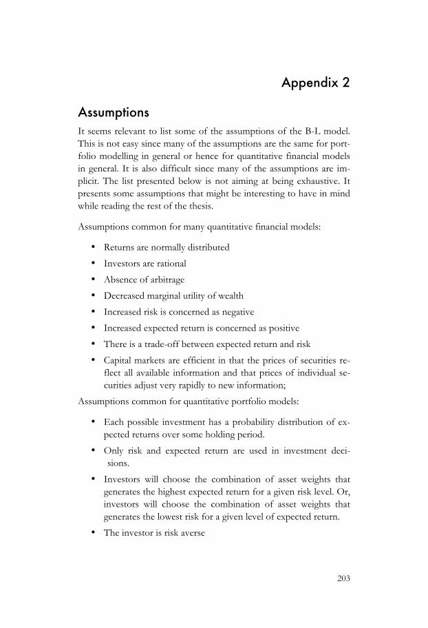
203

Appendix 2

Assumptions It seems relevant to list some of the assumptions of the B-L model. This is not easy since many of the assumptions are the same for port-folio modelling in general or hence for quantitative financial models in general. It is also difficult since many of the assumptions are im-plicit. The list presented below is not aiming at being exhaustive. It presents some assumptions that might be interesting to have in mind while reading the rest of the thesis.

Assumptions common for many quantitative financial models:

• Returns are normally distributed

• Investors are rational

• Absence of arbitrage

• Decreased marginal utility of wealth

• Increased risk is concerned as negative

• Increased expected return is concerned as positive

• There is a trade-off between expected return and risk

• Capital markets are efficient in that the prices of securities re-flect all available information and that prices of individual se-curities adjust very rapidly to new information;

Assumptions common for quantitative portfolio models:

• Each possible investment has a probability distribution of ex-pected returns over some holding period.

• Only risk and expected return are used in investment deci-sions.

• Investors will choose the combination of asset weights that generates the highest expected return for a given risk level. Or, investors will choose the combination of asset weights that generates the lowest risk for a given level of expected return.

• The investor is risk averse

204

• A portfolio's risk can be measured by the future variance of and the covariance between the assets’ rate of return.

• Taxes and other transaction costs like cuortage aren’t taken into account.

Assumptions specific to the B-L model:

• Investors have views about assets that they believe can lead to better performing portfolios

• The market isn’t totally efficient (Litterman, 2003).

• Risk ought to be taken in the assets to which investors have views

• Funds or portfolios are evaluated according to a benchmark portfolio.

• To every opinion a level-of-unconfidence must be estimated

205

Appendix 3

Behavioural Finance A more detailed description of the three parts within behavioural finance is given in the following. The description is not exhaustive but, hopefully, it will provide readers not familiar with the field of behavioural finance with an overview of the field and a feeling for its main ideas and research results. The overview will describe some central and well-established research results from the field.

The presentation begins with a description of “Limits to arbitrage”, one of the main parts of behavioural finance. Following this, “Heu-ristic-driven biases” and “Frame dependence” will be presented. These two parts of behavioural finance concern how psychological factors affect individual investors whereas the part “Limits to arbi-trage" is concerned with how psychology and “irrationality” affect markets.

Limits to arbitrage Whether markets behave “rationally” or not is the subject of a con-tinuous debate. . The efficient market hypothesis (EMH) has domi-nated economic theory since Fama (1970) presented the efficient financial theory as one in which securities are always priced in con-sideration of all available information. The efficient market hypoth-esis then states that real-world financial markets are efficient accord-ing to this definition. In the last 20 years this view of markets has been challenged. It is argued that the forces supposed to attain this efficiency, such as arbitrage trading, are likely to be much weaker than the defenders of the hypothesis claim (Shleifer, 2000). Behavioural finance, both theoretically and empirically, offers an alternative ap-proach. The efficient market hypothesis rests, according to Shleifer (2000), on three arguments relying on progressively weaker assump-tions:

1. Investors are assumed to be rational and hence to value securi-ties rationally.

206

2. If some investors are not rational, their irrational trades are random and therefore cancel each other out.

3. If investors should be acting irrationally in similar ways, ra-tional arbitrageurs act on the market and eliminate the influ-ence of irrational investors on prices.

A rational investor is, according to the EMH, defined as an investor who values securities on the basis of their fundamental value, the expected net present value of their future cash flows, discounted using their risk characteristics. According to EMH, rational investors only consider expected return and risk when evaluating investment strategies.

During the last 20 years, this view of markets has been challenged. It is argued that the forces that are supposed to attain the efficiency, such as arbitrage trading, are likely to be much weaker than the de-fenders of the hypothesis stress (Shleifer, 2000). Behavioural finance claims that errors, as they are discussed in EMH, are both systematic and significant and also that they can persist for long periods of time.

Let us begin by considering the first argument of EMH. It is difficult to sustain the belief that investors act fully rationally. Black (1986) shows that investors often trade on noise rather than on information, fail to diversify, sell winning securities and hold on to losers etc. Peo-ple deviate from the standard decision-making model in many essen-tial ways (Kahneman & Reipe, 1998). One of the most widely known examples of this is what Kahneman and Tversky (1979) call loss aver-sion, saying, among other things, that the value function is steeper for losses than for gains and that the value function is concave for losses and convex for gains. Kahneman and Tversky (1973) show that indi-viduals violate Bayes’ rule and other rules of probability theory. Kah-neman and Tversky (1979) also show that people assume that the empirical mean value of small and large samples has the same proba-bility distribution. This bias they refer to as the law of small numbers.

Kahneman and Tversky also question the second argument in the efficient market hypothesis, saying that irrational investors’ trades are random and therefore cancel each other. Kahneman and Tversky (1979) dispose this entirely by claiming that most often people devi-ate from rationality in the same way. For example investors are often

207

evaluated according to a benchmark and therefore often act to minimize the risk of falling behind. They also often act as a herd and select the same stock as other investment managers, again to avoid falling behind.

The last of the three arguments of the efficient market hypothesis says that even if the trades of noisy investors are correlated, arbi-trageurs act to bring prices back to their fundamental values. How-ever, researchers within behavioural finance claim that arbitrage trades are risky and because of this, limited. Arbitrage relies heavily on the existence of close substitutes. Yet, in many cases securities do not have good substitutes and therefore arbitrage trading cannot work to push prices back to fundamental values. For example an investor believing that stocks are overpriced cannot go short in stocks and buy a substitute portfolio. But even if there are almost perfect substitutes and the prices of the two securities ultimately con-verge, the trade may lead to temporary losses. Most arbitrageurs do not manage their own money; acting instead as agents for other peo-ple. These investors evaluate their portfolios regularly and quite fre-quently. If the evaluation horizon is shorter than the trade, the inves-tor may not be satisfied with the performance of the arbitrageur and therefore withdraw money. If many people withdraw money from the fund, the arbitrageur may have to liquidate the position, leading to further performance problems. These losses may result in the arbi-trageur being unable to maintain the position.

Empirical evidence supporting the efficient market hypothesis in the 1960s and 1970s was overwhelming. Shleifer (2000) divides the em-pirical evidences for the hypothesis into two categories. First, when news affecting the value of a security hits the market, it should quickly and correctly affect the price of the security. Quickly means that an in-vestor who receives the information late should not be able to profit from this information. Correctly, means that the price movement in response to the new information should be accurate on average. Sec-ond, since rational investors, according to the efficient market hy-pothesis, value securities on the basis of their fundamental value, prices should not be affected by changes in supply and demand of the security.

208

According to the first category money cannot be made on the basis of stale information. This argument is somewhat difficult to chal-lenge. To do this, we need to define the meaning of “stale information” and “making money”. “Making money” is hard to define. In finance “making money” means earning surplus returns after adjustment for risk. Showing that a strategy, based on stale information, earns on average a positive return is not enough to show market inefficiency. The profit may only be a fair market compensation for risk taking, but to evaluate this, we need a model for a fair relationship between risk and return etc. Still, when researchers suggest that they have found ways of “making money” on the basis of stale information, critics suggest that these profits are only fair compensation for risk-taking. One empirical result suggesting that information is not always quickly and correctly reflected in security prices is the so-called “Janu-ary effect”. Returns are seen to be superior in January, especially for small stocks but there is no evidence that stock or small stocks are riskier in January than the rest of the year.

According to the second category, rational investors only evaluate securities according to their fundamental values, meaning that chan-ges in demand or supply should not affect prices. Research has how-ever shown that prices react to inclusion of stocks in the Standard and Poor’s 500 Index (Shleifer, 2000). According to the efficient market hypothesis, inclusion of an asset in the Index is not supposed to convey any information to the market, but the asset price increases substantially and the increase is shown to be sustainable. According to Schole’s theory, inclusion of a security in an index should not af-fect its price because of increased demand. When the price of an asset begins to rise because of index inclusion the initial holders should want to sell and thereby stabilize the prices.

Heuristic-driven biases The other part of behavioural finance focuses on investor behaviour and psychology. Extensive empirical research within this field has shown that people do not always act according to the rational model as suggested by neoclassical theory. This, however, is probably not surprising. What is worth noting is that traditional economists have assumed that people differ from the rational model in a non-systematic way and therefore consider it impossible to incorporate

209

this in models. Behavioural finance claims to have found clear sys-tematic patterns in some of the ways in which people deviate from rational behaviour.

1974, the article Judgment under Uncertainty: Heuristics and Biases was published in the journal Science. It made a significant impression in the area of social sciences. The two authors, Amos Tversky and Daniel Kahneman, had written a number of articles on human judg-ment in the late 1960s and the early 1970s. This was the starting point in the field, within behavioural finance, often referred to as the Heu-ristics and biases approach to judgment under uncertainty. The core idea of the field is that complex probability judgments are often based on simplified heuristics instead of formal and extensive algorithms, as suggested by the rationality paradigm. This can give rise to series of systematic errors35, often referred to as biases. (Gilovich, Griffin & Kahneman, 2002). According to the heuristics and biases approach to judgment under uncertainty, people do not estimate likelihood and risk according to the laws of probability. Already in 1954, Paul Meehl compiled evidence saying that actuarial methods almost always out-performed expert predictions.

Kahneman and Tversky (1974) present three heuristics that give rise to a number of biases. These heuristics: representativeness, availab-ility, and anchoring and adjustment will be described below. It should however be mentioned that when reading literature regarding heu-ristic-driven biases, heuristics and biases are frequently not distin-guished (see for example Shefrin, 2002). Instead both heuristics and biases are referred to as heuristic-driven biases and hence representa-tiveness, availability, and anchoring and adjustment are also referred to as biases.

Heuristics

In this context, heuristics are the trial-and-error processes that lead people to develop rules of thumb. “It’s like back-of-the-envelope calcula-tions that sometimes come close to providing the right answer” (Shefrin, 2002, p.

35 Systematic errors is used within behavioural finance and refers to the systematic divergence of people from ”rational” behaviour according to homo economicus.

210

13). Heuristics help people reduce complex probability judgments into more simple judgment processes (Kahneman & Tversky, 1974). The use of heuristics is often advantageous, but it can give rise to some systematic errors, or biases.

Representativeness – Representativeness refers to judgments based on stereotypes. Kahneman and Tversky (1974) show that when people try to determine the probability that a model B generated a data set A or that an object D belongs to a class C, they often use the represen-tativeness heuristic. To illustrate, I will give an example of a bias de-rived from the representative heuristic referred to as base rate neglect. Tversky and Kahneman (1983) present this description of a person named Linda:

Linda is 31 years old, single, outspoken and very bright. She ma-jored in philosophy. As a student, she was deeply concerned with issues of discrimination and social justice and also partici-pated in anti-nuclear demonstrations.

When asked which of the statements “Linda is a bank teller” (statement A) and “Linda is a bank teller and is active in the feminist movement” (state-ment B) is more likely to be the correct statement, subjects typically assign greater probability to B. This is of course impossible since B is a subset from A. Here people fail to apply Bayes' law, saying that:

€

p(statementB description) =p(description statementB) p(statementB)

p(description)

People put too much weight on

€

p(description statementB) which cap-tures representativeness and too little weight on the base rate

€

p(statementB) . Representativeness provides a simple explanation. The description of Linda sounds like the description of a feminist – it is representative of a feminist – leading subjects to pick B. Represen-tativeness also leads to another bias, sample size neglect. People often fail to take the size of the sample into account. In situations where people do know the data-generating process in advance, the law of small numbers generates a gambler’s fallacy effect (see the section “Sample size neglect and the law of small numbers”).

211

Availability – When judging the probability of an event – say the like-lihood of getting mugged in Chicago – people often search in their memories for relevant information. While this is a perfectly sensible procedure, it can produce biased estimates because not all memories are equally retrievable or available. More recent events and more salient events – the mugging of a close friend in Chicago – will weight more heavily and distort the estimate. Whenever we use this kind of information and not only the frequency of the event, our assessment of the probability of the event will systematically be biased (Barberis & Thaler, 2003).

Anchoring and adjustment – Tversky and Kahneman (1974) argue that when forming estimates, people often start with some initial value and then adjust away from it. Experimental evidence shows that this is not beneficial. Tversky and Kahneman performed a test, asking two groups of subjects to estimate various percentages. Before de-termining their answers, a wheel of fortune was spun that settled at an arbitrary value. The student groups were then first asked to esti-mate whether their answer was lower or higher than the value on the wheel of fortune. After this they were asked to determine the final guess of the percentage. The median estimates of the percentage were 25 and 45 for the groups obtaining spin results of 10 and 65 respec-tively on the wheel of fortune. This indicates that the groups were affected by the value given by the wheel of fortune even though they knew it to be an arbitrary value.

Biases

The use of heuristics to solve complex problems can lead to system-atic errors. These errors are referred to as biases. The dictionary ex-planations of a bias are36: (1) “Bias: a personal and sometimes unreasoned judgment.” (2) “Bias: deviation of the expected value of a statistical estimate from the quantity it estimates.” (3) “Bias: systematic error introduced into sampling or testing by selecting or encouraging one outcome or answer over others.”

In the following, I will present three biases that are quite well estab-lished within behavioural finance.

36 www.merriam-webster.com

212

Overconfidence - People have been shown to be overconfident in their judgments. The confidence intervals people assign to their estimates of quantities are frequently far too narrow. Their 98% confidence intervals, for example, include the true quantity only about 60% of the time. People have also been shown to be poorly calibrated with respect to estimating probabilities: events they believe are certain to occur actually occur only approximately 80% of the time and events they deem impossible occur approximately 20% of the time. Accord-ing to Odean (1998b) overconfidence leads investors to trade too often and thereby reduce their returns.

Another is that, typically, over 90% of those surveyed think they are above average in such domains as driving skill, ability to get along with people and sense of humor.

DeBondt and Thaler (1995) state, “perhaps the most robust finding in the psychology of judgment is that people are overconfident.”

Most people are not as well-calibrated as they should be according to the efficient market hypothesis. They are overconfident and when they are overconfident, people set their confidence bands overly nar-row, setting their high guess too low and their low guess to high (She-frin, 2002). In a study by Werner DeBondt (1993) he finds that peo-ple tend to formulate their predictions by naively projecting trends that they perceive in the charts. He also found that people tend to be overconfident of their ability to predict accurately and that their con-fidence intervals are skewed, meaning that their best guesses do not lie midway between their low and high guesses (Shefrin, 2002, p. 51).

Conservatism - Once people have formed an opinion, they cling to it too tightly and for too long (Lord, Ross & Lepper, 1979). People are reluctant to search for evidence that contradicts their beliefs. Even if they find such evidence, they treat it with excessive skepticism. In the context of academic finance, belief perseverance predicts that if peo-ple begin believing in the Efficient Markets Hypothesis they may continue to believe in it long after compelling evidence to the con-trary has emerged.

While representativeness leads to an underweighting of base rates, there are situations in which base rates are over-emphasized relative

213

to sample evidence. In an experiment performed by Edwards (1968) there are two urns, one containing 3 blue balls and 7 red ones, and the other containing 7 blue balls and 3 red ones. A random draw of 12 balls with replacement from one of the urns yields 8 red and 4 blue. What is the probability that the draw was made from the first urn? While the correct answer is 0.97, most people estimate a number around 0.7, thus overweighting the base rate of 0.5. It appears that if a data sample is representative of an underlying model, people react too little to the data and rely too much on their prior information.

Sample size neglect or the law of small numbers - Sample size neglect origi-nates from the representative heuristic. Research has shown that people assess the same probability distribution to the empirical mean value of small and large samples. The phenomenon is related to the under-use of base rates. By this people expect close to the same probability distribution of types in small groups as they do in large groups. People also exaggerate the likelihood that a short sequence of flips of a fair coin will yield roughly the same number of heads as tails (Rabin, 1998). 1969 Kahneman and Frederick performed a study on 84 participants at meetings of the Mathematical Psychology Society and the American Psychological Association (Tversky & Kahneman, 1971). The respondents were asked realistic questions about the ro-bustness of statistical estimates and the reliability of research results. The survey showed a belief that the law of large numbers applies to small numbers as well. The respondents showed little sensitivity to sample size and therefore placed too much confidence in the results of small samples. Most of the respondents had the capability to easily compute the correct answers, hence they had access to two distinct approaches for answering statistical questions, one spontaneous and fast, and one rule-governed, laborious and slow. These results raised questions about the educability of statistical intuition.

A concept known as “the gambler’s fallacy” is regarded as a manifesta-tion of the law of small numbers. If a fair coin has not come up tails after 2-3 tosses, people think it is “due” for a tails, because a sequen-ces of flips with a fair coin ought to result in nearly as many tails as heads. The fallacy leads people to over-infer the probability distribu-tion from short sequences (Rabin, 1998).

214

One more implication of the law of small number is that people ex-pect too few lengthy strikes (series of associated events) in a random sequence. This has been shown in several tests. Most series imagined by subject contains too many short sequences of the same events and hence too few long sequences of the same event. (Falk & Konold, 1997). In basketball there is a widespread belief in the “hot hand” phenomenon. This implies that a particular basketball player has “on” nights, when he or she plays very well, and “off” nights, when he or she plays poorly. It is not believed that these “on” and “off” nights can be explained by randomness. Gilovich, Vallone and Tversky (1985) and Tversy and Gilovich (1989) have argued that this phe-nomenon does not exist. The “hot hand” idea can be explained by the problems we have in believing in lengthy strikes (Rabin, 1998).

Home Bias – Investors might tend to overweight domestic assets be-cause the domestic stocks and markets feels more familiar and are maybe often are more familiar than the foreign ones Availability or saliency that drives home bias (Massa & Simonov, 2003). People focus heavily on information that is salient or is often mentioned.

Frame dependence According to traditional the framing of a problem should not affect the behaviour of investors. The framing of financial problems should always be transparent investors. However, researchers within behav-ioural finance have obtained convincing research results implying that people are, in fact, sensitive to the framing of problems.

The disposition effect – The disposition effect is one of the results of extending prospect theory to investments. It builds on the S-shaped value function of prospect theory. The disposition effect refers to the tendency of investors to hold losers too long and to sell winners too soon. Consider an investor who holds two stocks, one is up and the other is down. If the investor has a liquidity problem, she/he is more likely to sell the stock that is up (Odean, 1998a). Investors are thus disposed toward realizing their gains but not selling their losers. The disposition effect is similar to the overconfidence hypothesis but where overconfidence is market-wide and implies an increase in trad-ing volume; the disposition effect is stock-specific (Statman & Thor-ley, 2001).

215

Mental Accounting – It has been shown that individuals and households divide their wealth into mental accounts to organize their financial activities. One example that I believe many people might recognize is the winning of money on a gamble. When money is won on a gam-ble, it is quite common for people to mentally put this money in a specific account to be spent on further gambling.

Prospect Theory – In the mid-seventies Tversky and Kahneman pre-sented a new theory called Prospect Theory. Prospect theory builds on the results from research performed on judgment under uncertainty and on frame dependence. Prospect theory asks questions on how consumer choices are formed by probabilities and related outcomes (Laibson & Zeckhauser, 1998). According to Kahneman and Tversky (1979), prospect theory is to be considered as an alternative model to the expected utility theory. According to Shiller (1998), prospect theory is probably the behavioural theory that has had the most influ-ence on economic research. Rabin (1998) also gives prospect theory the second place, after expected utility theory, as the most frequent subject for research in economics.

It is well known that human behaviour systematically deviates from that predicted by expected utility theory (Shiller, 1998). Kahneman and Tversky (1979) demonstrate how people systematically violate the theory:

First, subjects were asked to choose between buying tickets in two lotteries. One lottery offered a 25% chance of winning 3,000 and the other lottery offered a 20% chance of winning 4,000. When choosing between these two lotteries, 65% of the subjects chose the latter. Second, subjects were asked to choose between two other lotteries, offering a 100% chance of winning 3,000 and an 80% chance of win-ning 4,000. 80% chose the former lottery (loss aversion). According to expected utility theory people should be indifferent to these two pairs of lotteries because the choices are the same except that the probabilities (25% and 20%) are multiplied by the same constant (4) in the second pair of lotteries. This example illustrates what is called “certainty effect”, the fact that people have a preference for out-comes, which are certain.

216

Prospect theory is a mathematical theory that is said to capture the results from experimental outcomes and is to be considered as an alternative to the expected utility maximization. Prospect theory is similar in some ways to expected utility theory. In prospect theory “individuals are represented as maximizing a weighted sum of ‘utilities’, although the weights are not the same as probabilities and the ‘utilities’ are determined by what they call a ‘value function’ rather than a utility function” (Shiller 1998, p. 4). Shiller also suggests that by substituting the Kahneman and Tver-sky weights for the probabilities in expected utility theory, a number of puzzling phenomena in observed human behaviour in relation to risk might be explained. Shiller claims that the Kahneman-Tversky value function can explain overpricing of out-of-the-money and in-the-money options. The options smile might be explained in terms of the distortion in probabilities represented by the Kahneman-Tversky value function since prospect theory suggests that people act as if they overestimate the small probability that the price of the under-lying crosses the strike price and underestimate the high probability that the price remains on the same side of the strike price (Shiller, 1998).

The shape of the value function differs between prospect theory and expected utility theory. In prospect theory the value function is:

Figure A.3 Utility function suggested in behavioural finance

1. Defined on losses and gains instead on total wealth

Value

Losses Gains

217

2. Concave in the domain of gains and convex in the domain of losses

3. Considerably steeper for losses than for gains

4. The kink at the reference point (origin)

Loss Aversion – An important concept both within behavioural finance as a field and in prospect theory is Loss aversion. Loss aversion is an expression of the unwillingness of many people to bet on a fair coin and is implied by the kink and the difference in the slope of the value function of prospect theory. Research has shown that the attractive-ness of winning € X is not nearly sufficient to compensate for the risk of loosing the same amount. Risk aversion has played a central role in economic theory. Loss aversion however implies that the value func-tion is convex in the domains of losses, see figure 6.2, and therefore represents a risk-seeking behaviour in the case of loss. Consider a situation in which a person must choose from a sure loss off €800 and an 85% risk of loosing €1000 . Most people would accept the 85% risk of loosing €1000 instead of the sure loss. This is a risk-seeking behaviour. Risk-seeking behaviour has been confirmed by several investigations. “A person who has not made peace with her/his losses is likely to accept gambles that would be unacceptable to her /him otherwise” (Kahneman & Tversky, 1979). Loss aversion accounts for the en-dowment effect and the status quo bias. The Status quo bias means that individuals tend to remain at the status quo because of the asym-metry in the utility function. The endowment effect means that people are prone to demand more to give up an object than they are to acquire the same object. For a more elaborative explanation of the status quo bias and the endowment effect please see 0. Regret can also be associated with loss aversion. On making a mistake that could have been avoided, individuals tend to feel regret. Research has shown that the fear of regretting a decision affects the behaviour of individuals. Regret is also, in some sense, embodied in the utility function of behavioural finance.

218

Appendix 4

Reflections on Organizational Structure This section was a part of the concluding chapter of the licentiate thesis, that was constituted of step one and two of this thesis.

The chapter served as a preview of and starting point for further work in the subject of the thesis.

Organizational structure and the B-L model Ideas concerning the organization of the use of a model such as the B-L have arisen during the two first steps. These ideas will be pre-sented and discussed generally in the following. They will serve as initial thoughts and concepts for the following studies.

Who should set weight-on-views? The dilemma with overconfidence when stating the levels-of-unconfidence in the B-L model might be solved to some extent with a well-designed and well-functioning organization. When reading existing literature concerning the B-L, it can be considered that it is assumed that the same person should state both the unconfidence levels and the weight-on-views. The organizational discussion within the literature regarding the B-L model is, as mentioned, limited. It is stated that parameters should be set, but not how nor by whom. That some parameters might be difficult to set in any way is not men-tioned. It should be possible however, and might be interesting to consider whether one person could state the views and the levels-of-unconfidence allocated to each view while another person sets the weight-on-views. The person setting the weight-on-views could for example be the fund manager’s boss. The boss can then focus more on studying the fund managers, who they are, how they have per-formed and how well they may be able to estimate future returns and unconfidence levels. If an inexperienced investor has been fortunate and performed very well for some months, he/she may become overconfident, attributing his/her success to his/her own skills rather than to chance (see 6.2). If the boss notes this, he/she has a tool with which to cope with the overconfidence of the fund manager. The boss can lower the weight-on-views and thereby reduce the impact of

219

the overconfidence of the fund manager on the portfolio. Evaluating fund managers in this way may appear quite difficult, but it may be an interesting way to use the model. It has been said above that behav-ioural finance has shown that humans are bad at estimating their own level-or-unconfidence. I have found no research results indicating whether people are good or bad at estimating the confidence levels of others.

Decision groups Both behavioural finance and portfolio theory often refer to “the investor”. I find it interesting to consider the appearance of a team managing a fund using the B-L model. My, so far, limited experience in practical fund management makes it difficult for me to envisage such a team. The complexity of managing a fund with the help of an advanced quantitative tool such as the B-L model, would, I believe, demand a group of individuals with different positions and special knowledge. The team can be seen as a “dream team” based on im-pressions I have gained during my research. The team could consist of the following participants:

1. Asset analysts who analyze in detail the assets the portfolio or fund contains.

2. A macro specialist focused in macro economic prognosis and the effects of macro economic events.

3. A risk specialist focused on future risk and hence not only on the ARCHing, GARCHing and EGARCHing (expression from Frankfurte,r 1994) of historical time series, but on risk forecasts, forecasts of covariances and variances.

4. A B-L specialist focused in the model itself and in the particu-lar implementation of the model used in the organization.

5. A boss or group leader who is specialized in economic phi-losophy and organizational issues - The group leader could be specialized in organizational questions and also have know-ledge about economic philosophical questions. The group leader might be able to widen the group’s viewpoint and per-haps reduce the risk of the group following un-fruitful per-spectives.

220

These are examples of roles in a fund management team that seems appealing. For allocation of the portfolio I imagine a meeting be-tween these specialists presenting their knowledge, prognoses and ideas of asset returns, risks and macro economic events during the following investment period. A dynamic discussion involving all these persons would increase the probability that data input to the B-L model would be as well thought through as possible. The team could then, together, evaluate the reasonability of the portfolio output by the model. The team members could test different inputs and investi-gate how these would affect the output portfolio. It is an interesting question to what degree this way of working would be fruitful and rewarding.

221

Appendix 5

Empirical Material Interviews with portfolio managers (around 1 h each): • 20060619 – (recorded and transcribed)

• 20060621–(recorded and transcribed)

• 20060621 (recorded and transcribed)

• 20061020 – (recorded)

• 20061107 – (recorded)

• 20061218 – (recorded)

Empirical material collected at SIB: The time spent working with the BLImp, BLOld, SIBLImp outside SIB and the listed meeting is deemed to be about 480 hours.

Interviews (around 1 h each):

• 20061108 – John (recorded and transcribed)

• 20061213 – Pete (recorded and transcribed)

Meetings (between 45 min – 2h):

• 20070509 – John & Charlotta

• 20070516 – Pete & Charlotta (recorded and transcribed)

• 20070524 – Pete, Tom & Charlotta (recorded and transcribed)

• 20071023 – John, & Charlotta (recorded and transcribed):

• 20071031 – John, Tom & Charlotta (recorded and tran-scribed):

• 20071212 – John & Charlotta (recorded and transcribed):

• 20080226 – John & Charlotta (recorded and transcribed):

• 20080305 – John, Tom & Charlotta, three others from the VM group*

• 20080416 – John & Charlotta*

• 20080424 – John & Charlotta (recorded and transcribed)

• 20090310 – Eric & Charlotta

222

• 20101015 – Eric & Charlotta

* Not recorded and transcribed because of technological failures

Allocation:

• 20080822 – Eric, Bill & Charlotta (3h)

• 20080825 – Eric Bill & Charlotta (3h)

• 20080923 – Eric, Bill & Charlotta (3h)

Printouts from SIBLImp and note taken during the meetings

Programs – B-L Implementations:

• BLOld

• BLImp

• SIBLImp

223

Appendix 6

Alternative Finance In this thesis the term “Alternative finance” is used as an umbrella concept to the alternative financial research with critical approaches towards modern finance. Traditional financial theory is often referred to as modern finance and the term postmodern finance would thus seem appropriate as an umbrella. However, the stigma and com-plexity of post-modernity impede the use of this term here. The de-scription of alternative finance is divided in six sections: Anti-modern finance, Behavioural finance, Real-world economics (formerly Post-autistic economics), Social studies of finance, Organizational finance, and Critical finance studies. It should be noted that the way to pres-ent alternative finance has not been given. Since the streams are simi-lar and sometimes difficult to separate from each other, the main point should be clarified and that is that there are a number of movements that wish to change and/or supplement traditional finan-cial research. They aim to change the way traditional financial re-search is performed today and are therefore all called alternative fi-nance.

The ways in which alternative finance aims to change financial re-search vary however. While some are more uniting, striving to expand existing financial research, others are quite polemic, motivated to totally reform the way traditional financial research ought to be per-formed. For the record, I would like to elucidate my position on this issue. My belief is that mainstream finance would benefit from ex-pansion with more qualitative research that takes social, cultural and organizational contexts into consideration. However, I would not throw out the child with the bathwater and will not make assertions as to whether current mainstream finance fails in other respects or not.

Ideas within alternative finance have served as sources of inspiration in the third study of this thesis.

224

Anti-modern finance There is no research field or stream that refers to itself as “anti-modern finance”. However, there is a discussion concerning short-comings of the modern assumptions within traditional economic theory. Anti-Modernism is a label borrowed from McCloskey (1998), who is strongly critical of the modernist approach within modern economics.

Frankfurter et. al. (1997) actually uses the term post-modern finance and claims that:

Modernity begins with things (objects) and the properties of the things, and the purpose of science is to discover the facts about them; that is, laws that govern how properties change and how things relate. In post-modernity, what is important is how things and so-called facts are used within culture, which, of course, changes as culture changes. In modernity, there is an in-herent meaning to objects; in post-modernity, the meaning lies in their appearances.

(Frankfurter et. al., 1997, p. 2)

McGoun maintains that post-modern finance differs from modern finance in the sense that while modern finance seeks to discover re-ality, post-modern finance believes that reality is not there to be dis-covered but is instead something that is constructed: “We don’t discover finance; we invent finance” (Frankfurter et. al., 1997, p. 148).

Frankfurter criticizes modern finance for its lack of communication with individuals and argues that the worst aspect of modernity is that research draws conclusions about the motivation of individuals with-out talking to people about what their motivations are (Frankfurter, 1997, p.228).

McCloskey points out that today’s (1998) economics journals appear more to be journals in applied mathematics or statistics. According to McCloskey, there is no doubt that modernism is the leading paradigm of mainstream finance “In any case, modernism rules: that is the main point.” (McCloskey, 1998, p. 147). She also argues that the modernist starting point prevents traditional economics from creating useful and usable knowledge “A modernist methodology consistently applied, in other words,

225

would stop advances in economics” (McCloskey, 1998, p. 154). She con-cludes by claiming:

In 1953 the modernist fairy tale in methodology looked coura-geously up to date, suited to a band of revolutionaries in the mountains. By now, in part because its revolution has been suc-cessful, it looks oppressive, suited to a government in the coastal plains, squatting on the major ports and the radio sta-tion. Economists are not alone in adhering to the modernist revolution so long after its spirit has died. Perhaps it will be comforting to know that they would also not be alone if they repudiated its excesses.

(McCloskey, 1998, p. 155)

As indicated, anti-modern finance is quite polemic in character, aim-ing as it does to revolutionize the field of economics.

Behavioural finance When presenting alternative fields of financial research it is difficult to exclude behavioural finance. Behavioural finance is the financial field, taking another social science into account, that has earned greatest acceptance by traditional financial theory. This might be related to the tendency within behavioural finance to allow itself to be assimilated by traditional finance (Frankfurter & McGoun, 2002). Behavioural finance is quite thoroughly presented and discussed in part II and will therefore not be discuss further here.

Real-world economics A movement referred to as “real-world economics” has taken form during the last decade. In the year 2000, a group of students related to France’s ‘Grandees Coles’ distributed a manifesto on the Internet protesting against what they considered to be a lack of realism in economics. The called the movement “post-autistic economics” be-cause “allegiance to a single narrative necessarily means that in the main it refuses to look at economic reality” (Fullbrook, 2005). In 2008, the name was changed to real-world economics. Real-world economics protests against the way mathematics is used within economics with the result that economics has become an “autistic science”. In their manifesto the students demanded a change in the teaching of the subject that would leave room for critical and reflective thoughts. The real-world economics movement now involves thousands of economists all over

226

the world who wish to free economics from the neoclassical ap-proach as the only approach to economics and introduce pluralistic thinking to the theory.

Bondio (2003)37 suggests the following foundations for a new eco-nomic theory:

• “Bring both consumer and producer analysis together through the analysis of people

• Require less emphasis on mathematical logic and more on ob-serving reality

• Shift methodology towards group analysis away from individu-alism

• Require explicit historical perspectives when analyzing the de-velopment and emergence of groups and their norms.”

One of real-world economics’ major tasks is to work for pluralism and critical thinking within the field of finance. It is therefore pos-sible to argue that research within the fields introduced below may be presented as input to real-world economics.

Social studies of finance Social studies of finance (SSF) uses methods within social sciences to study financials markets. Anthropology, gender studies, geography, history, politics, social studies of science, socio-legal studies, and sociology are used within the field. Social studies of finance aims to become a multidisciplinary field where researchers from different disciplines can interact and exchange experiences (MacKenzie, 2010). Donald MacKenzie holds a professorial fellowship to carry out social studies of finance and he claims:

To understand the creation, development and effects of finan-cial markets we need more than the perspectives of economics or of a ‘behavioural’ finance that is rooted in individual psy-chology. Markets are cultures.

(MacKenzie, 2010, http://www.sociology.ed.ac.uk/finance/about.htm)

37 http://www.paecon.net/PAEReview/issue19/Bondio19.htm

227

de Goede concludes that social studies of finance is and ought to be a flexible research programme. Social studies of finance should be:

…an interdisciplinary forum for discussion and debate, enabling dialogue and disagreement between researchers in a diversity of disciplines who share a fascination for money, and who may otherwise not have easily engaged.

(de Goede, 2005, p. 25)

According to de Goede (2005), one of the most important aspects of social studies of finance is the opening of the “late-modern ‘black box’ of financial statistics, models and technology”. According to MacKenzie (2005a) the only way of opening a black box is to interact with those involved in its construction. de Goede (2005) articulates three “con-cerns” central to the field of social studies of finance. These are:

• Resocialisation of financial practices – Populate abstract financial models with social human creatures.

• Performativity – Meaning that economic theory itself contributes to the construction of the phenomena it de-scribes.

• Repoliticisation of financial practices – Writing cultural histories and opening the black boxes shows that markets and money are socially constructed.

Social studies of finance is a constellation of different research areas, which use different approaches and methodologies for studying fi-nancial markets, organizations and people. Methods borrowed from sociology such as field studies and anthropological and ethnographi-cal methods, among others, are used. Benunza and Stark (2004) con-duct ethnographic field research on arbitrage trading in the Wall Street trading room of a major international investment bank. Will-man et. al. (2002) make a field study on loss aversion at an investment bank. MacKenzie (2005b) studies and analyzes arbitrage by using the Long Term Capital Management38 crash as an example. Through interviews MacKenzie shows how social context is of importance when it comes to arbitrage trading.

38 Long Term Capital Management was a large hedge fund that after a couple of years of incred-ible return to investors crashed in 1998.

228

As indicated by the quote by de Goede above, social studies of fi-nance are more open and uniting and aim to expand the field of fi-nance in relation to anti-modern finance.

Organizational finance While normative questions are absent in social studies of finance, organizational finance takes both normative business-administrative and purely descriptive sociological problems into consideration. Blomberg (2005) introduces organizational finance and declares that such research is closely related to social studies of finance. When it comes to theoretical starting points and tools the differences between organizational finance and social studies of finance are almost non-existent. It is important to note that, unlike the other fields described, organizational finance is not exactly a research stream. Organizational finance is rather a compilation of Blomberg’s thoughts and ideas about what organizational research has to say about the stock market and its actors.

When describing the research Blomberg (2005) says that there are no pure paradigms and that it cannot be claimed that it is more reward-ing to be pragmatic and orthodox than to move between different paradigms. As long as analyses are based on conscious choices and a reasonably high level of theory, Blomberg maintains that both nor-mative and descriptive research are of importance. A constructionist perspective is essential to research within organizational finance and also the analysis of actors’ thoughts and actions both between the actors themselves and between the actors and artifacts. It is important that power perspective and processes of influence are taken into ac-count in organizational finance research. Bloomberg asserts that both individual motives and interests and the constructional process of identities need to be analyzed.

Blomberg motivates the practical relevance of organizational finance by claiming that organizational finance, in contrast to traditional fi-nance, can show that development is not spontaneous but depends on active actors.

229

Critical finance studies Forslund (2008) emphasizes that there is no critical stream of finance research. There is, however, a stream of research that refers to itself as “Critical Finance Studies”. On their website they claim:

Our mission is putting philosophy and art to work on financial ideas, theories and practices, in order to create concepts that will make it possible to think and use finance altogether differ-ently.

(www.criticalfinancestudies.org, 2010 May 6)

By critical finance studies we are implying an attempt at bring-ing radically new insights and experiences into the study of fi-nance.

(www.criticalfinancestudies.org, 2010 May 6, Call for Papers Critical Finance Studies Conference II)

Critical finance studies have arranged at least two conferences. It is interesting that MacKenzie (Social Studies of Finance), McGoun (anti-modern or post modern finance) and Forslund (referred to at the beginning of this chapter) all attended and spoke at the 2009 con-ference. This elucidates the fact discussed above that the streams presented here are similar and not clearly separated from each other.

Keasey and Hudson (2007) aim to introduce a field of critical finance. They criticize traditional finance as being closed and not taking the outside world into account. In that sense, they portray traditional finance rather harshly as “a house without windows”.

Rather than attempting to see the actions of individuals at first hand or indeed engage in debate with those individuals who are actually involved in financial decisions, the community prefers to stay safe in its ‘house without windows’ and take data feeds from the outside world.

(Keasey & Hudson, 2007, p. 933)

The researchers discuss different problems of ‘puzzles’ of traditional asset allocation or portfolio choice. The difference between portfolio construction in theory and practice is used as an example of the prob-lems in modern finance. According to theory all investors ought to hold the same mix of risky assets, assuming they can invest in a risk-free asset and hence vary the risk return characteristics of the port-

230

folio by shifting the weight of the risk-free asset. However, according to Canner et. al. (1997) financial advisors seem not to recommend this way of investing. Instead they adjust the risk in customers’ port-folios by balancing between bonds and stocks (considered risky assets in by Canner et al., whereas cash is considered the risk-free asset). This difference between financial theory and practice is, by traditional finance, called a ‘puzzle’. An obvious way of approaching such a ‘puzzle’, according to Hudson and Keasey, would be to interact with financial advisors and analyze why they act in this way. However, the question is instead analyzed by attempting to modify existing core assumptions, which could be done without interacting with practi-tioners. The ‘puzzle’ was not solved and in 2007 was still an open question.

Hudson and Keasey examine whether customers also believe that shifting the riskiness of a portfolio is done by shifting the weights of bonds in relation to stocks in a portfolio. According to the authors this seems to be the case. They argue that the fact that customers and the financial advisors seem to use the same method to change the riskiness of a portfolio implies that the:

…advisors are giving a structure of advice which mirrors the beliefs of the clients.

(Keasey & Hudson, 2007, p. 942)

Keasey and Hudson call for research that investigates “action, behav-iours and interactions” on the part of financial market participants. Re-search that builds on grounded theory, observer participation, focus groups, open interviews, structured questionnaires, data analysis in-cluding longitudinal series, experimental methods and more are sorely needed in financial research. Like Forslund (2008), Keasey and Hud-son points at the fact that for this kind of research to be done there need to exist journals accepting such research. There are few journals that accept such papers and, as mentioned earlier, the ones that do are not traditional financial journals. Critical Perspectives in Account-ing is a journal that actually does this. Keasey and Hudson, however, suggest and wonder whether a sister journal called Critical Perspec-tives in Finance, hence focusing on such research, could be launched.