the blinder-oaxaca decomposition for linear regression...

The Stata Journal (2008)8, Number 4, pp. 453–479

The Blinder–Oaxaca decomposition for linearregression models

Ben JannETH Zurich

Zurich, [email protected]

Abstract. The counterfactual decomposition technique popularized by Blinder(1973, Journal of Human Resources, 436–455) and Oaxaca (1973, InternationalEconomic Review, 693–709) is widely used to study mean outcome differences be-tween groups. For example, the technique is often used to analyze wage gaps bysex or race. This article summarizes the technique and addresses several compli-cations, such as the identification of effects of categorical predictors in the detaileddecomposition or the estimation of standard errors. A new command called oaxaca

is introduced, and examples illustrating its usage are given.

Keywords: st0151, oaxaca, Blinder–Oaxaca decomposition, outcome differential,wage gap

1 Introduction

An often used methodology to study labor-market outcomes by groups (sex, race, andso on) is to decompose mean differences in log wages based on linear regression modelsin a counterfactual manner. The procedure is known in the literature as the Blinder–Oaxaca decomposition (Blinder 1973; Oaxaca 1973). It divides the wage differentialbetween two groups into a part that is “explained” by group differences in produc-tivity characteristics, such as education or work experience, and a residual part thatcannot be accounted for by such differences in wage determinants. This “unexplained”part is often used as a measure for discrimination, but it also subsumes the effects ofgroup differences in unobserved predictors. Most applications of the technique can befound in the labor market and discrimination literature (for meta studies, see, e.g.,Stanley and Jarrell [1998] or Weichselbaumer and Winter-Ebmer [2005]). However, themethod can also be useful in other fields. In general, the technique can be employedto study group differences in any (continuous and unbounded1) outcome variable. Forexample, O’Donnell et al. (2008) use it to analyze health inequalities by poverty status.

The purpose of this article is to introduce a new Stata command, called oaxaca, thatimplements the Blinder–Oaxaca decomposition. In the next section, the most commonvariants of the decomposition are summarized, and a number of issues, such as theidentification of the contribution of categorical predictors or the estimation of standarderrors, are addressed. The third section then describes the syntax and options of the

1. See Sinning, Hahn, and Bauer (in this issue) for the decomposition of group differences in categor-ical or bounded outcomes.

c© 2008 StataCorp LP st0151

454 The Blinder–Oaxaca decomposition for linear regression models

new oaxaca command, and the fourth section uses labor-market data to illustrate itsapplications.

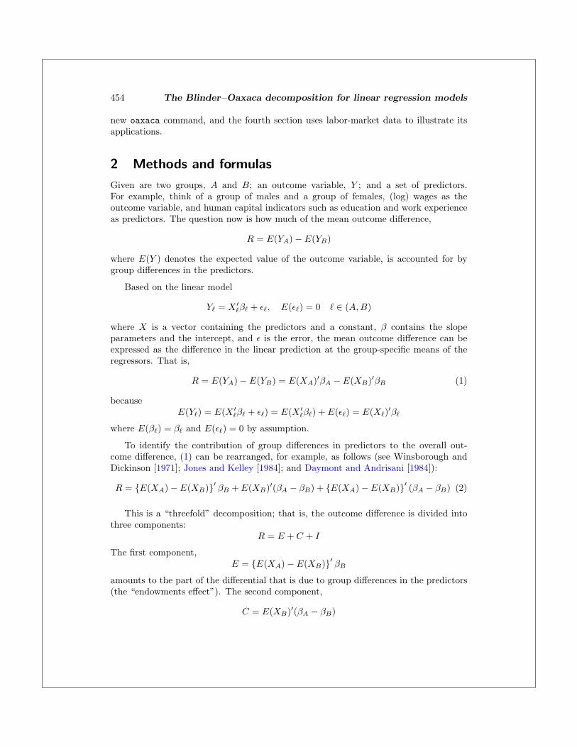
2 Methods and formulas

Given are two groups, A and B; an outcome variable, Y ; and a set of predictors.For example, think of a group of males and a group of females, (log) wages as theoutcome variable, and human capital indicators such as education and work experienceas predictors. The question now is how much of the mean outcome difference,

R = E(YA) − E(YB)

where E(Y ) denotes the expected value of the outcome variable, is accounted for bygroup differences in the predictors.

Based on the linear model

Y� = X ′�β� + ε�, E(ε�) = 0 � ∈ (A,B)

where X is a vector containing the predictors and a constant, β contains the slopeparameters and the intercept, and ε is the error, the mean outcome difference can beexpressed as the difference in the linear prediction at the group-specific means of theregressors. That is,

R = E(YA) − E(YB) = E(XA)′βA − E(XB)′βB (1)

becauseE(Y�) = E(X ′

�β� + ε�) = E(X ′�β�) + E(ε�) = E(X�)′β�

where E(β�) = β� and E(ε�) = 0 by assumption.

To identify the contribution of group differences in predictors to the overall out-come difference, (1) can be rearranged, for example, as follows (see Winsborough andDickinson [1971]; Jones and Kelley [1984]; and Daymont and Andrisani [1984]):

R = {E(XA) − E(XB)}′ βB + E(XB)′(βA − βB) + {E(XA) − E(XB)}′ (βA − βB) (2)

This is a “threefold” decomposition; that is, the outcome difference is divided intothree components:

R = E + C + I

The first component,E = {E(XA) − E(XB)}′ βB

amounts to the part of the differential that is due to group differences in the predictors(the “endowments effect”). The second component,

C = E(XB)′(βA − βB)

B. Jann 455

measures the contribution of differences in the coefficients (including differences in theintercept). And the third component,

I = {E(XA) − E(XB)}′ (βA − βB)

is an interaction term accounting for the fact that differences in endowments and coef-ficients exist simultaneously between the two groups.

The decomposition shown in (2) is formulated from the viewpoint of group B. Thatis, the group differences in the predictors are weighted by the coefficients of group B todetermine the endowments effect (E). The E component measures the expected changein group B’s mean outcome if group B had group A’s predictor levels. Similarly, forthe C component (the “coefficients effect”), the differences in coefficients are weightedby group B’s predictor levels. That is, the C component measures the expected changein group B’s mean outcome if group B had group A’s coefficients. Naturally, thedifferential can also be expressed from the viewpoint of group A, yielding the reversethreefold decomposition,

R = {E(XA) − E(XB)}′ βA + E(XA)′(βA − βB) − {E(XA) − E(XB)}′ (βA − βB) (3)

Now the endowments effect amounts to the expected change of group A’s mean outcomeif group A had group B’s predictor levels. The coefficients effect quantifies the expectedchange in group A’s mean outcome if group A had group B’s coefficients.

An alternative decomposition prominent in the discrimination literature results fromthe concept that there is a nondiscriminatory coefficient vector that should be usedto determine the contribution of the differences in the predictors. Let β∗ be such anondiscriminatory coefficient vector. The outcome difference can then be written as

R = {E(XA) − E(XB)}′ β∗ + {E(XA)′(βA − β∗) + E(XB)′(β∗ − βB)} (4)

We now have a “twofold” decomposition,

R = Q + U

where the first component,

Q = {E(XA) − E(XB)}′ β∗

is the part of the outcome differential that is explained by group differences in thepredictors (the “quantity effect”), and the second component,

U = E(XA)′(βA − β∗) + E(XB)′(β∗ − βB)

is the unexplained part. The latter is usually attributed to discrimination, but it isimportant to recognize that it also captures all the potential effects of differences inunobserved variables.


The unexplained part in (4) is sometimes further decomposed. Let βA = β∗ + δA

and βB = β∗ + δB , with δA and δB as group-specific discrimination parameter vectors(positive or negative discrimination, depending on the sign). U can then be expressedas

U = E(XA)′δA − E(XB)′δB

That is, the unexplained component of the differential can be subdivided into a part,

UA = E(XA)′δA

that measures discrimination in favor of group A and a part,

UB = −E(XB)′δB

that quantifies discrimination against group B.2 Again, however, this interpretationhinges on the assumption that there are no relevant unobserved predictors.

The estimation of the components of the threefold decompositions shown in (2) and(3) is straightforward. Let βA and βB be the least-squares estimates for βA and βB ,obtained separately from the two group-specific samples. Furthermore, use the groupmeans XA and XB , as estimates for E(XA) and E(XB). Based on these estimates, (2)and (3) are computed as

R = Y A − Y B = (XA − XB)′βB + X′B(βA − βB) + (XA − XB)′(βA − βB)

and

R = Y A − Y B = (XA − XB)′βA + X′A(βA − βB) − (XA − XB)′(βA − βB)

The determination of the components of the twofold decomposition shown in (4)is more involved because an estimate for the unknown nondiscriminatory coefficientsvector β∗ is needed. Several suggestions have been made in the literature. For example,there may be reason to assume that discrimination is directed toward only one of thegroups, so that β∗ = βA or β∗ = βB (see Oaxaca [1973], who speaks of an “index numberproblem”). Again assume that members of group A are males and members of groupB are females. If, for instance, wage discrimination is directed only against women andthere is no (positive) discrimination of men, then we can use βA as an estimate for β∗

and compute (4) asR = (XA − XB)′βA + X

′B(βA − βB) (5)

Similarly, if there is only (positive) discrimination of men but no discrimination ofwomen, the decomposition is

R = (XA − XB)′βB + X′A(βA − βB) (6)

Often, however, there is no specific reason to assume that the coefficients of one orthe other group are nondiscriminating. Moreover, economists have argued that the

2. UA and UB have opposite interpretations. A positive value for UA reflects positive discriminationof group A; a positive value for UB indicates negative discrimination of group B.

B. Jann 457

undervaluation of one group comes along with an overvaluation of the other (e.g., Cotton[1988]). Reimers (1983) therefore proposes using the average coefficients over bothgroups as an estimate for the nondiscriminatory parameter vector; that is,

β∗ = 0.5βA + 0.5βB

Similarly, Cotton (1988) suggests to weight the coefficients by the group sizes, nA andnB ; that is,

β∗ =nA

nA + nBβA +

nB

nA + nBβB

Furthermore, based on theoretical derivations, Neumark (1988) advocates the use of thecoefficients from a pooled regression over both groups as an estimate for β∗.

As pointed out by Oaxaca and Ransom (1994) and others, (4) can also be expressedas

R = {E(XA) − E(XB)}′ {WβA + (I − W)βB}+ {(I − W)′E(XA) + W′E(XB)}′ (βA − βB)

where W is a matrix of relative weights given to the coefficients of group A, and I is theidentity matrix. For example, choosing W = I is equivalent to setting β∗ = βA. Simi-larly, W = 0.5I is equivalent to β∗ = 0.5βA +0.5βB . Furthermore, Oaxaca and Ransom(1994) show that

W = Ω = (X′AXA + X′

BXB)−1X′AXA (7)

with X as the observed data matrix is equivalent to using the coefficients from a pooledmodel over both groups as the reference coefficients.3

An issue with the approach by Neumark (1988) and Oaxaca and Ransom (1994) isthat it can inappropriately transfer some of the unexplained parts of the differential intothe explained component, although this does not seem to have received much attentionin the literature.4 Assume a simple model of log wages (ln W ) on education (Z) withthe sex-specific intercepts αM and αF due to discrimination. The model is

ln W ={

αM + γZ + ε, if “male”αF + γZ + ε, if “female”

3. Another solution is to set W = diag(β − βB) × diag(βA − βB)−1, where β without a subscriptdenotes the coefficients from the pooled model. Although the decomposition results are the same,this approach yields a weighting matrix that is quite different from Oaxaca and Ransom’s (1994)Ω. For example, whereas W computed as described in this footnote is a diagonal matrix, Ω hasoff-diagonal elements that are unequal to zero and are not even symmetric.

4. An exception is Fortin (2006).


Let αM = α and αF = α + δ, where δ is the discrimination parameter. Then the modelcan also be expressed as

ln W = α + γZ + δF + ε

with F as an indicator for “female”. Assume that γ > 0 (positive relation betweeneducation and wages) and δ < 0 (discrimination against women). If we use γ∗ from apooled model,

ln W = α∗ + γ∗Z + ε∗

in (4), then following from the theory on omitted variables (see, e.g., Gujarati [2003,510–513]), the explained part of the differential is

Q = {E(ZM ) − E(ZF )} γ∗ = {E(ZM ) − E(ZF )}{

γ + δCov(Z,G)

Var(Z)

}where Var(Z) is the variance of Z, and Cov(Z,G) is the covariance between Z and G.If men on average are better educated than women, then the covariance between Z andG is negative, and the explained part of the decomposition gets overstated (given γ > 0and δ < 0). In essence, the difference in wages between men and women is explainedby sex.

To avoid such a distortion of the decomposition results because of the residual groupdifference spilling over into the slope parameters of the pooled model, my recommen-dation is to always include a group indicator in the pooled model as an additionalcovariate.

Estimation of sampling variances

Given the popularity of the Blinder–Oaxaca procedure, it is astonishing how little at-tention has been paid to the issue of statistical inference. Most studies in which theprocedure is applied only report point estimates for the decomposition results and donot make any indications about sampling variances or standard errors.5 However, foran adequate interpretation of the results, approximate measures of statistical precisionare indispensable.

Approximate variance estimators for certain variants of the decomposition were firstproposed by Oaxaca and Ransom (1998), with Greene (2008, 55–56) making similarsuggestions. The estimators by Oaxaca and Ransom (1998) and Greene (2008) are agood starting point, but they neglect an important source of variation. Most social-science studies on discrimination are based on survey data where all (or most of) thevariables are random variables. That is, not only the outcome variable but also the pre-dictors are subject to sampling variation (an exception would be experimental factorsset by the researcher). Whereas an important result for regression analysis is that it doesnot matter for the variance estimates whether regressors are stochastic or fixed, this is

5. Exceptions are, for example, Oaxaca and Ransom (1994, 1998), Silber and Weber (1999),Horrace and Oaxaca (2001), Fortin (2006), Heinrichs and Kennedy (2007), and Lin (2007). Fur-thermore, Jackson and Lindley (1989) and Shrestha and Sakellariou (1996) propose statistical testsfor discrimination.

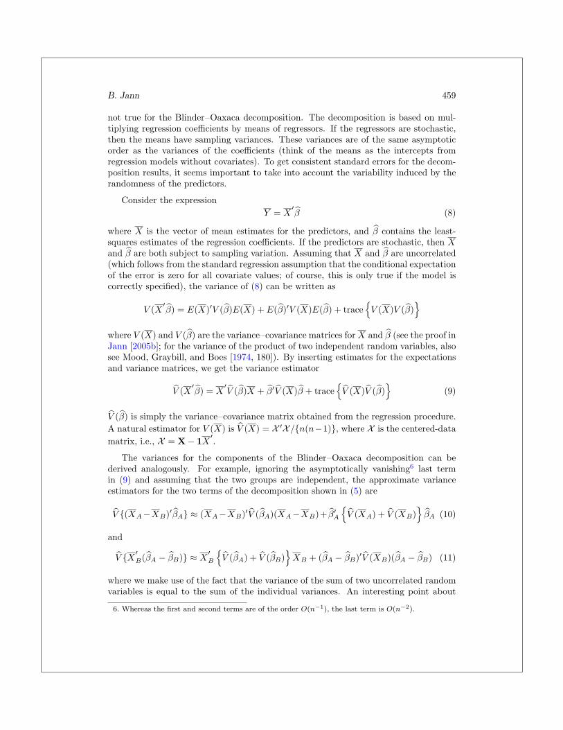
B. Jann 459

not true for the Blinder–Oaxaca decomposition. The decomposition is based on mul-tiplying regression coefficients by means of regressors. If the regressors are stochastic,then the means have sampling variances. These variances are of the same asymptoticorder as the variances of the coefficients (think of the means as the intercepts fromregression models without covariates). To get consistent standard errors for the decom-position results, it seems important to take into account the variability induced by therandomness of the predictors.

Consider the expressionY = X

′β (8)

where X is the vector of mean estimates for the predictors, and β contains the least-squares estimates of the regression coefficients. If the predictors are stochastic, then Xand β are both subject to sampling variation. Assuming that X and β are uncorrelated(which follows from the standard regression assumption that the conditional expectationof the error is zero for all covariate values; of course, this is only true if the model iscorrectly specified), the variance of (8) can be written as

V (X′β) = E(X)′V (β)E(X) + E(β)′V (X)E(β) + trace

{V (X)V (β)

}where V (X) and V (β) are the variance–covariance matrices for X and β (see the proof inJann [2005b]; for the variance of the product of two independent random variables, alsosee Mood, Graybill, and Boes [1974, 180]). By inserting estimates for the expectationsand variance matrices, we get the variance estimator

V (X′β) = X

′V (β)X + β′V (X)β + trace

{V (X)V (β)

}(9)

V (β) is simply the variance–covariance matrix obtained from the regression procedure.A natural estimator for V (X) is V (X) = X ′X/{n(n−1)}, where X is the centered-datamatrix, i.e., X = X − 1X

′.

The variances for the components of the Blinder–Oaxaca decomposition can bederived analogously. For example, ignoring the asymptotically vanishing6 last termin (9) and assuming that the two groups are independent, the approximate varianceestimators for the two terms of the decomposition shown in (5) are

V {(XA−XB)′βA} ≈ (XA−XB)′V (βA)(XA−XB)+ β′A

{V (XA) + V (XB)

}βA (10)

and

V {X ′B(βA − βB)} ≈ X

′B

{V (βA) + V (βB)

}XB + (βA − βB)′V (XB)(βA − βB) (11)

where we make use of the fact that the variance of the sum of two uncorrelated randomvariables is equal to the sum of the individual variances. An interesting point about

6. Whereas the first and second terms are of the order O(n−1), the last term is O(n−2).


(10) and (11) is that ignoring the stochastic nature of the predictors will primarily affectthe variance of the first term of the decomposition (the explained part). This is becausein most applications group differences in coefficients and means are much smaller thanthe levels of coefficients and means.

It is possible to develop similar formulas for all the decomposition variants outlinedabove, but derivations can get complicated once a pooled model is used and covariancesbetween the pooled model and the group models have to be taken into account. Likewise,derivations can get complicated if the assumption of independence between the twogroups is loosened (e.g., if dealing with a cluster sample). An alternative approach thatis simple and general and produces equivalent results is to estimate the joint variance–covariance matrix of all used statistics (see Weesie [1999] and [R] suest) and then applythe “delta method” (see [R] nlcom and the references therein). In fact, for independencebetween the two groups, the results of the delta method for (2) are formally equal to(10) and (11). Furthermore, a general result for the delta method is that if the inputvariance matrix is asymptotically normal, then the variance matrix of the transformedstatistics is asymptotically normal (see, e.g., Greene [2008, 68–71]). That is, becauseasymptotic normality holds for regression coefficients and mean estimates under verygeneral conditions, the variances obtained by the delta method can be used to constructapproximate confidence intervals for the decomposition results in the usual manner.

Detailed decomposition

Often, not only is the total decomposition of the outcome differential into an explainedand an unexplained part of interest, but also the detailed contributions of the singlepredictors or sets of predictors are subject to investigation. For example, one might wantto evaluate how much of the gender wage gap is due to differences in education and howmuch is due to differences in work experience. Similarly, it might be informative todetermine how much of the unexplained gap is related to differing returns to educationand how much is related to differing returns to work experience.

Identifying the contributions of the individual predictors to the explained part ofthe differential is easy because the total component is a simple sum over the individualcontributions. For example, in (5),

Q = (XA − XB)′βA = (X1A − X1B)β1A + (X2A − X2B)β2A + · · ·

where X1,X2, . . . are the means of the single regressors, and β1, β2, . . . are the associ-ated coefficients. The first summand reflects the contribution of the group differences inX1; the second, of differences in X2; and so on. Also the estimation of standard errorsfor the individual contributions is straightforward.

Similarly, using (5) as an example, the individual contributions to the unexplainedpart are the summands in

U = X′B(βA − βB) = X

′1B(β1A − β1B) + X

′2B(β2A − β2B) + · · ·

B. Jann 461

However, other than for the explained part of the decomposition, the contributionsto the unexplained part can depend on arbitrary scaling decisions if the predictors do nothave natural zero points (e.g., Jones and Kelley [1984, 334]). Without loss of generality,assume a simple model with just one explanatory variable:

Y� = β0� + β1�Z� + ε�, � ∈ (A,B)

The unexplained part of the decomposition based on (5) then is

U = (β0A − β0B) + (β1A − β1B)ZB

The first summand is the part of the unexplained gap that is due to “group member-ship” (Jones and Kelley 1984); the second summand reflects the contribution of differingreturns to Z. Now assume that the zero point of Z is shifted by adding a constant, a.The effect of such a shift on the decomposition results is as follows:

U ={

(β0A − aβ1A) − (β0B − aβ1B)}

+ (β1A − β1B)(ZB + a)

Evidently, the scale shift changes the results; a portion amounting to a(β1A− β1B) istransferred from the group membership component to the part that is due to differentslope coefficients. The conclusion is that the detailed decomposition results for theunexplained part have a meaningful interpretation only for variables for which scaleshifts are not allowed, that is, for variables that have a natural zero point.7

A related issue that has received much attention in the literature is that the de-composition results for categorical predictors depend on the choice of the omittedbase category (Jones 1983; Jones and Kelley 1984; Oaxaca and Ransom 1999; Nielsen2000; Horrace and Oaxaca 2001; Gardeazabal and Ugidos 2004; Polavieja 2005; Yun2005b). The effect of a categorical variable is usually modeled by including 0/1 vari-ables (“dummy” variables) for the different categories in the regression equation, whereone of the categories (the “base” category) is omitted to avoid collinearity. It is easy tosee that the decomposition results for the single 0/1 variables depend on the choice ofthe base category, because the associated coefficients quantify differences with respectto the base category. If the base category changes, the decomposition results change.

For the explained part of the decomposition, this may not be critical because thesum of the contributions of the single indicator variables (that is, the total contribu-tion of the categorical variable) is unaffected by the choice of the base category. Forthe unexplained part of the decomposition, however, there is again a tradeoff betweenthe group membership component (the difference in intercepts) and the part attributed

7. The problem does not occur for the explained part of the decomposition or the interaction compo-nent in the threefold decomposition because a cancels out in these cases. Furthermore, stretchingor compressing the scales of the X variables (multiplication by a constant) does not alter any ofthe decomposition results because such multiplicative transformations are counterbalanced by thecoefficient estimates.


to differences in slope coefficients. For the unexplained part, changing the base cat-egory not only alters the results for the single dummy variables but also changes thecontribution of the categorical variable as a whole.

An intuitively appealing solution to the problem has been proposed by Gardeazabaland Ugidos (2004) and Yun (2005b). The idea is to restrict the coefficients for the singlecategories to sum to zero, that is, to express effects as deviations from the grand mean.This can be implemented by restricted least-squares estimation or by transforming thedummy variables before model estimation, as proposed by Gardeazabal and Ugidos(2004).8 A more convenient method in the context of the Blinder–Oaxaca decom-position is to estimate the group models by using the standard dummy coding and thentransform the coefficient vectors so that deviations from the grand mean are expressedand the (redundant) coefficient for the base category is added (Suits 1984; Yun 2005b).If applied to such transformed estimates, the results of the Blinder–Oaxaca decomposi-tion are independent of the choice of the omitted category. Furthermore, the results areequal to the simple averages of the results one would get from a series of decompositionsin which the categories are used one after another as the base category (Yun 2005b).

The deviation contrast transform works as follows. Given is the model

Y = β0 + β1D1 + · · · + βk−1Dk−1 + ε

where β0 is the intercept, and Dj , j = 1, . . . , k−1, are the dummy variables representinga categorical variable with k categories. Category k is the base category. Alternatively,the model can be formulated as

Y = β0 + β1D1 + · · · + βk−1Dk−1 + βkDk + ε

where βk is constrained to zero. Now let

c = (β1 + · · · + βk)/k

and defineβ0 = β0 + c and βj = βj − c, j = 1, . . . , k

The transformed model is then

Y = β0 + β1D1 + · · · + βkDk + ε,

k∑j=1

βj = 0

The transformed model is mathematically equivalent to the untransformed model. Forexample, the two models produce identical predictions. The variance–covariance matrixfor the transformed model can be obtained by applying the general formula for weightedsums of random variables given in, e.g., Mood, Graybill, and Boes (1974, 179). Modelswith several sets of dummy variables can be transformed by applying the formulas toeach set separately. Furthermore, the transformation can be applied to the interaction

8. In fact, the approach by Gardeazabal and Ugidos (2004) is simply what is known as the “effectscoding” (Hardy 1993, 64–71) or the “deviation contrast coding” (Hendrickx 1999) approach.

B. Jann 463

terms between a categorical and a continuous variable in an analogous manner exceptthat now c is added to the main effect of the continuous variable instead of the intercept.The application of the transform is not restricted to linear regression. It can be usedwith any model as long as the effects of the dummies are expressed as additive effects.

Other restrictions to identify the contribution of a categorical variable to the unex-plained part of the decomposition are imaginable. For example, the restriction couldbe

k∑j=1

wj βj = 0

where wj are weights proportional to the relative frequencies of the categories, so thecoefficients reflect deviations from the overall sample mean (Kennedy 1986; Haisken-DeNew and Schmidt 1997). Hence, there is still some arbitrariness in the method byGardeazabal and Ugidos (2004) and Yun (2005b).

3 The oaxaca command

The methods presented above are implemented with a new command called oaxaca.The command first estimates the group models and possibly a pooled model over bothgroups using regress ([R] regress) or any user-specified estimation command. suest([R] suest) is then applied, if necessary, to determine the combined variance–covariancematrix of the models, and the group means of the predictors are estimated by usingmean ([R] mean). Finally, the various decomposition results and their standard errors(and covariances) are computed based on the combined parameter vector and variance–covariance matrix of the models’ coefficients and the mean estimates.9 The standarderrors are obtained by the delta method.10

9. The covariances between the models’ coefficients and the mean estimates are assumed to be zeroin any case. This assumption can be violated in misspecified models.

10. nlcom ([R] nlcom) could be used to compute the variance–covariance matrix of the decompositionresults. However, nlcom employs general methods based on numerical derivatives and is slow if themodels contain many covariates. oaxaca therefore has its own specific implementation of the deltamethod based on analytic derivatives.


3.1 Syntax

The syntax of the oaxaca command is

oaxaca depvar[indepvars

] [if] [

in] [

weight], by(groupvar)

[swap

detail[(dlist)

]adjust(varlist) threefold

[(reverse)

]weight(#

[#. . .

])

pooled[(model opts)

]omega

[(model opts)

]reference(name) split

x1(names and values) x2(names and values) categorical(clist)

svy[([vcetype

] [, svy options

])]vce(vcetype) cluster(varname)

fixed[(varlist)

] [no]suest nose model1(model opts) model2(model opts)

noisily xb level(#) eform nolegend]

where depvar is the outcome variable of interest (e.g., log wages) and indepvars arepredictors (e.g., education, work experience). groupvar identifies the groups to be com-pared. oaxaca typed without arguments replays the last results.

fweights, aweights, pweights, and iweights are allowed; see [U] 11.1.6 weight.Furthermore, bootstrap, by, jackknife, statsby, and xi are allowed; see [U] 11.1.10prefix, commands. Weights are not allowed with the bootstrap prefix, and aweightsare not allowed with the jackknife prefix. vce(), cluster(), and weights are notallowed with the svy option.

3.2 Options

Main

by(groupvar) specifies the groupvar that defines the two groups to be compared. by()is required.

swap reverses the order of the groups.

detail[(dlist)

]specifies that the detailed results for the individual predictors be re-

ported. Use dlist to subsume the results for sets of regressors (results for variablesnot appearing in dlist are listed individually). The syntax for dlist is

name:varlist[, name:varlist . . .

]The usual shorthand conventions apply to the varlists specified in dlist (see helpvarlist; additionally, cons is allowed). For example, specify detail(exp:exp*)to subsume exp (experience) and exp2 (experience squared). name is any valid Stataname; it labels the set.

adjust(varlist) causes the differential to be adjusted by the contribution of the specifiedvariables before performing the decomposition. This is useful, for example, if thespecified variables are selection terms. adjust() is not needed for heckman models.

B. Jann 465

Decomposition type

threefold[(reverse)

]computes the threefold decomposition. This is the default

unless weight(), pooled, omega, or reference() is specified. The decompositionis expressed from the viewpoint of group 2 (B). Specify threefold(reverse) toexpress the decomposition from the viewpoint of group 1 (A).

weight(#[# ...

]) computes the twofold decomposition, where #

[# ...

]are the

weights given to group 1 (A) relative to group 2 (B) in determining the referencecoefficients (weights are recycled if there are more coefficients than weights). Forexample, weight(1) uses the group 1 coefficients as the reference coefficients, andweight(0) uses the group 2 coefficients.

pooled[(model opts)

]computes the twofold decomposition by using the coefficients

from a pooled model over both groups as the reference coefficients. groupvar isincluded in the pooled model as an additional control variable. Estimation detailscan be specified in parentheses; see the model1() option below.

omega[(model opts)

]computes the twofold decomposition by using the coefficients from

a pooled model over both groups as the reference coefficients (excluding groupvaras a control variable in the pooled model). Estimation details can be specified inparentheses; see the model1() option below.

reference(name) computes the twofold decomposition by using the coefficients from astored model. name is the name under which the model was stored; see [R] estimatesstore. Do not combine the reference() option with the bootstrap or jackknifemethods.

split causes the unexplained component in the twofold decomposition to be split intoa part related to group 1 (A) and a part related to group 2 (B). split is effectiveonly if specified with weight(), pooled, omega, or reference().

Only one of threefold, weight(), pooled, omega, and reference() is allowed.

X-values

x1(names and values) and x2(names and values) provide custom values for specificpredictors to be used for group 1 (A) and group 2 (B) in the decomposition. Thedefault is to use the group means of the predictors. The syntax for names and valuesis

varname[=]

value[ [

,]

varname[=]

value . . .]

For example, x1(educ 12 exp 30).


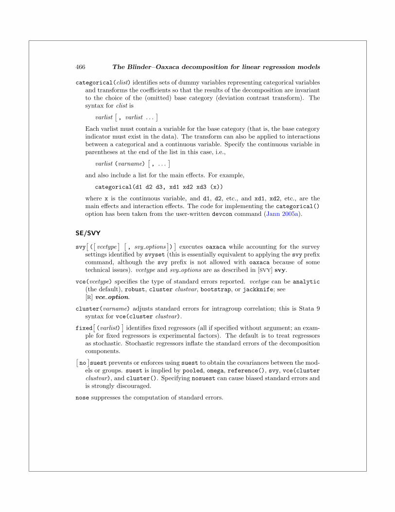
categorical(clist) identifies sets of dummy variables representing categorical variablesand transforms the coefficients so that the results of the decomposition are invariantto the choice of the (omitted) base category (deviation contrast transform). Thesyntax for clist is

varlist[, varlist . . .

]Each varlist must contain a variable for the base category (that is, the base categoryindicator must exist in the data). The transform can also be applied to interactionsbetween a categorical and a continuous variable. Specify the continuous variable inparentheses at the end of the list in this case, i.e.,

varlist (varname)[, . . .

]and also include a list for the main effects. For example,

categorical(d1 d2 d3, xd1 xd2 xd3 (x))

where x is the continuous variable, and d1, d2, etc., and xd1, xd2, etc., are themain effects and interaction effects. The code for implementing the categorical()option has been taken from the user-written devcon command (Jann 2005a).

SE/SVY

svy[([vcetype

] [, svy options

])]

executes oaxaca while accounting for the surveysettings identified by svyset (this is essentially equivalent to applying the svy prefixcommand, although the svy prefix is not allowed with oaxaca because of sometechnical issues). vcetype and svy options are as described in [SVY] svy.

vce(vcetype) specifies the type of standard errors reported. vcetype can be analytic(the default), robust, cluster clustvar, bootstrap, or jackknife; see[R] vce option.

cluster(varname) adjusts standard errors for intragroup correlation; this is Stata 9syntax for vce(cluster clustvar).

fixed[(varlist)

]identifies fixed regressors (all if specified without argument; an exam-

ple for fixed regressors is experimental factors). The default is to treat regressorsas stochastic. Stochastic regressors inflate the standard errors of the decompositioncomponents.[

no]suest prevents or enforces using suest to obtain the covariances between the mod-

els or groups. suest is implied by pooled, omega, reference(), svy, vce(clusterclustvar), and cluster(). Specifying nosuest can cause biased standard errors andis strongly discouraged.

nose suppresses the computation of standard errors.

B. Jann 467

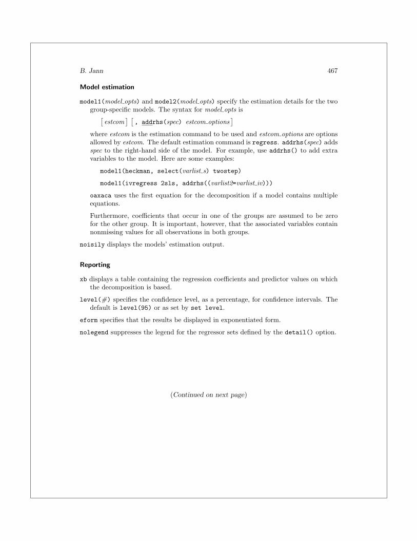
Model estimation

model1(model opts) and model2(model opts) specify the estimation details for the twogroup-specific models. The syntax for model opts is[

estcom] [

, addrhs(spec) estcom options]

where estcom is the estimation command to be used and estcom options are optionsallowed by estcom. The default estimation command is regress. addrhs(spec) addsspec to the right-hand side of the model. For example, use addrhs() to add extravariables to the model. Here are some examples:

model1(heckman, select(varlist s) twostep)

model1(ivregress 2sls, addrhs((varlist2=varlist iv)))

oaxaca uses the first equation for the decomposition if a model contains multipleequations.

Furthermore, coefficients that occur in one of the groups are assumed to be zerofor the other group. It is important, however, that the associated variables containnonmissing values for all observations in both groups.

noisily displays the models’ estimation output.

Reporting

xb displays a table containing the regression coefficients and predictor values on whichthe decomposition is based.

level(#) specifies the confidence level, as a percentage, for confidence intervals. Thedefault is level(95) or as set by set level.

eform specifies that the results be displayed in exponentiated form.

nolegend suppresses the legend for the regressor sets defined by the detail() option.

(Continued on next page)


3.3 Saved results

Scalarse(N) number of observations e(N 1) number of obs. in group 1e(N clust) number of clusters e(N 2) number of obs. in group 2

Macrose(cmd) oaxaca e(legend) definitions of regressor setse(depvar) name of dependent variable e(adjust) names of adjustment variablese(by) name of group variable e(fixed) names of fixed variablese(group 1) value defining group 1 e(suest) suest, if suest was usede(group 2) value defining group 2 e(wtype) weight typee(title) title in estimation output e(wexp) weight expressione(model) type of decomposition e(clustvar) name of cluster variablee(weights) weights specified in weight() e(vce) vcetype specified in vce()e(refcoefs) equation name used in e(b0) e(vcetype) title used to label Std. Err.

for the reference coefficients e(properties) b Ve(detail) detail, if detailed results

were requested

Matricese(b) decomposition results e(b0) coefficients and X-valuese(V) variance matrix of e(b) e(V0) variance matrix of e(b0)

Functionse(sample) marks estimation sample

4 Examples

Threefold decomposition

The standard application of the Blinder–Oaxaca technique is to divide the wage gapbetween, say, men and women into a part that is explained by differences in determinantsof wages, such as education or work experience, and a part that cannot be explainedby such group differences. An example using data from the Swiss Labor Market Survey1998 (Jann 2003) is as follows:

. use oaxaca, clear(Excerpt from the Swiss Labor Market Survey 1998)

. oaxaca lnwage educ exper tenure, by(female) noisily

Model for group 1

Source SS df MS Number of obs = 751F( 3, 747) = 101.14

Model 49.613308 3 16.5377693 Prob > F = 0.0000Residual 122.143834 747 .163512495 R-squared = 0.2889

Adj R-squared = 0.2860Total 171.757142 750 .229009522 Root MSE = .40437

lnwage Coef. Std. Err. t P>|t| [95% Conf. Interval]

educ .0820549 .0060851 13.48 0.000 .070109 .0940008exper .0098347 .0016665 5.90 0.000 .0065632 .0131062

tenure .0100314 .0020397 4.92 0.000 .0060272 .0140356_cons 2.24205 .0778703 28.79 0.000 2.08918 2.394921

B. Jann 469

Model for group 2

Source SS df MS Number of obs = 683F( 3, 679) = 40.34

Model 33.5197344 3 11.1732448 Prob > F = 0.0000Residual 188.08041 679 .276996185 R-squared = 0.1513

Adj R-squared = 0.1475Total 221.600144 682 .324926897 Root MSE = .5263

lnwage Coef. Std. Err. t P>|t| [95% Conf. Interval]

educ .0877579 .0087108 10.07 0.000 .0706546 .1048611exper .0131074 .0028971 4.52 0.000 .0074191 .0187958

tenure .0036577 .0035374 1.03 0.301 -.0032878 .0106032_cons 2.097806 .1091691 19.22 0.000 1.883457 2.312156

Blinder-Oaxaca decomposition Number of obs = 1434

1: female = 02: female = 1

lnwage Coef. Std. Err. z P>|z| [95% Conf. Interval]

DifferentialPrediction_1 3.440222 .0174874 196.73 0.000 3.405947 3.474497Prediction_2 3.266761 .0218522 149.49 0.000 3.223932 3.309591

Difference .1734607 .027988 6.20 0.000 .1186052 .2283163

Decomposit~nEndowments .0852798 .015693 5.43 0.000 .0545222 .1160375

Coefficients .082563 .0255804 3.23 0.001 .0324263 .1326996Interaction .005618 .010966 0.51 0.608 -.0158749 .0271109

As is evident from the example, oaxaca first estimates two group-specific regressionmodels and then performs the decomposition (the noisily option causes the groupmodels’ results to be displayed and is specified in the example for illustration). Thedefault decomposition performed by oaxaca is the threefold decomposition (2). Tocompute the reverse threefold decomposition (3), specify threefold(reverse).

The decomposition output reports the mean predictions by groups and their dif-ference in the first panel. In our sample, the mean of log wages (lnwage) is 3.44 formen and 3.27 for women, yielding a wage gap of 0.17. In the second panel of the de-composition output, the wage gap is divided into three parts. The first part reflectsthe mean increase in women’s wages if they had the same characteristics as men. Theincrease of 0.085 in the example indicates that differences in years of education (educ),work experience (exper), and job tenure (tenure) account for about half the wage gap.The second term quantifies the change in women’s wages when applying the men’s co-efficients to the women’s characteristics. The third part is the interaction term thatmeasures the simultaneous effect of differences in endowments and coefficients.


Twofold decomposition

Alternatively, the twofold decomposition (4) can be requested, where weight(), pooled,or omega determines the choice of the reference coefficients. For example, weight(1)corresponds to (5), and weight(0) corresponds to (6). omega causes the coefficientsfrom a pooled model over both samples to be used as the reference coefficients, whichis equivalent to Oaxaca and Ransom’s approach based on (7). The pooled option alsocauses the coefficients from a pooled model to be used, but now the pooled model alsocontains a group membership indicator. Based on the argumentation outlined in section2, my suggestion is to use pooled rather than omega.

For our example data, the results after using the pooled option are as follows:

. oaxaca lnwage educ exper tenure, by(female) pooled



Robustlnwage Coef. Std. Err. z P>|z| [95% Conf. Interval]


Difference .1734607 .0279325 6.21 0.000 .118714 .2282075

Decomposit~nExplained .089347 .0137531 6.50 0.000 .0623915 .1163026

Unexplained .0841137 .025333 3.32 0.001 .034462 .1337654

Again the conclusion is that differences in endowments account for about half the wagegap.11

A further possibility is to provide a stored reference model by using the reference()option. For example, for the decomposition of the wage gap between blacks and whites,the reference model is sometimes estimated based on all races, not just blacks and whites.Then the reference model would have to be estimated first using all observations andthen be provided to oaxaca via the reference() option.

Exponentiated results

The results in the example above are expressed on the logarithmic scale (remember thatlog wages are used as the dependent variable), and it might be sensible to retransformthe results to the original scale (here Swiss francs) by using the eform option:

11. Unlike the first example, robust standard errors are reported (oaxaca uses suest to estimate thejoint variance matrix for all coefficients if pooled is specified; suest implies robust standard errors).To compute robust standard errors in the first example, you would have to add vce(robust) to thecommand.

B. Jann 471

. oaxaca, eform



Robustlnwage exp(b) Std. Err. z P>|z| [95% Conf. Interval]


Difference 1.189414 .0332234 6.21 0.000 1.126048 1.256346

Decomposit~nExplained 1.09346 .0150385 6.50 0.000 1.064379 1.123336

Unexplained 1.087753 .027556 3.32 0.001 1.035063 1.143125

The (geometric) means of wages are 31.2 Swiss francs for men and 26.2 Swiss francs forwomen, which amounts to a difference of 18.9%. Adjusting women’s endowments levelsto the levels of men would increase women’s wages by 9.3%. A gap of 8.8% remainsunexplained.

Survey estimation

oaxaca supports complex survey estimation, but svy has to be specified as an optionand is not allowed as a prefix command (which does not restrict functionality). Forexample, the wt variable provides sampling weights for the Swiss Labor Market Survey1998. The weights (and strata or primary sampling units [PSUs], if there were any) canbe taken into account as follows:



. svyset [pw=wt]

pweight: wtVCE: linearized

Single unit: missingStrata 1: <one>

SU 1: <observations>FPC 1: <zero>

. oaxaca lnwage educ exper tenure, by(female) pooled svy

Blinder-Oaxaca decomposition

Number of strata = 1 Number of obs = 1647Number of PSUs = 1647 Population size = 1657.1804

Design df = 1646


Linearizedlnwage Coef. Std. Err. t P>|t| [95% Conf. Interval]


Difference .2118488 .035728 5.93 0.000 .1417718 .2819259

Decomposit~nExplained .1107614 .0189967 5.83 0.000 .0735011 .1480216

Unexplained .1010875 .0315911 3.20 0.001 .0391246 .1630504

Detailed decomposition

Use the detail option to compute the individual contributions of the predictors tothe components of the decomposition. detail specified without argument reports thecontribution of each predictor individually. Alternatively, one can define groups ofpredictors for which the results can be subsumed in parentheses. Furthermore, one mightapply the deviation contrast transform to dummy-variable sets so that the contributionof a categorical predictor to the unexplained part of the decomposition does not dependon the choice of the base category. For example,

B. Jann 473

. tabulate isco, nofreq generate(isco)

. oaxaca lnwage educ exper tenure isco2-isco9, by(female) pooled> detail(exp_ten: exper tenure, isco: isco?) categorical(isco?)



Robustlnwage Coef. Std. Err. z P>|z| [95% Conf. Interval]


Difference .1734607 .0279331 6.21 0.000 .118713 .2282085

Explainededuc .0395615 .0097334 4.06 0.000 .0204843 .0586387

exp_ten .0399316 .0089081 4.48 0.000 .022472 .0573911isco -.0056093 .012445 -0.45 0.652 -.0300009 .0187824Total .0738838 .017772 4.16 0.000 .0390513 .1087163

Unexplainededuc -.1324971 .1788045 -0.74 0.459 -.4829475 .2179533

exp_ten .0129955 .0400811 0.32 0.746 -.0655619 .0915529isco -.0159367 .0296549 -0.54 0.591 -.0740592 .0421858_cons .2350152 .195018 1.21 0.228 -.1472132 .6172435Total .0995769 .0266887 3.73 0.000 .047268 .1518859

exp_ten: exper tenureisco: isco1 isco2 isco3 isco4 isco5 isco6 isco7 isco8 isco9

Differences in education and combined differences in experience and tenure each ac-count for about half the explained part of the outcome differential, whereas occupationalsegregation based on the nine major groups of the International Standard Classificationof Occupations (ISCO-88) does not seem to matter much.

Selectivity bias adjustment

In labor-market research, it is common to include a correction for sample-selectionbias in the wage equations based on the procedure by Heckman (1976, 1979). Wagesare observed only for people who are participating in the labor force, and this mightbe a selective group. The most straightforward approach to account for selectionbias in the decomposition is to deduct the selection effects from the overall differen-tial and then apply the standard decomposition formulas to this adjusted differential(Reimers [1983]; an alternative approach is followed by Dolton and Makepeace [1986];see Neuman and Oaxaca [2004] for an in-depth treatment of this issue).



If oaxaca is used with heckman, the decomposition is automatically adjusted for se-lection. For example, the following command includes a selection correction in the wageequation for women and decomposes the adjusted wage gap. Labor-force participation(lfp) is modeled as a function of age, age squared, marital status, and the number ofchildren at ages 6 or below and at ages 7 to 14.

. oaxaca lnwage educ exper tenure, by(female) model2(heckman, twostep> select(lfp = age agesq married divorced kids6 kids714))





Difference .164579 .0331442 4.97 0.000 .0996176 .2295404



Comparing the results with the output in the first example reveals that the uncorrectedwages of women are slightly biased downward (3.267 versus the selectivity-corrected3.276), and the wage gap is somewhat overestimated (0.173 versus the corrected 0.165).

It is sometimes sensible to compute the selection variables outside of oaxaca and thenuse the adjust() option to correct the differential (although here the selection variablesare assumed known, which might slightly bias the standard errors). For example,

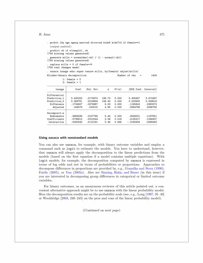
B. Jann 475

. probit lfp age agesq married divorced kids6 kids714 if female==1

(output omitted )

. predict xb if e(sample), xb(759 missing values generated)

. generate mills = normalden(-xb) / (1 - normal(-xb))(759 missing values generated)

. replace mills = 0 if female==0(759 real changes made)

. oaxaca lnwage educ exper tenure mills, by(female) adjust(mills)





Difference .1734607 .0279987 6.20 0.000 .1185843 .2283372Adjusted .164579 .033215 4.95 0.000 .0994788 .2296792



Using oaxaca with nonstandard models

You can also use oaxaca, for example, with binary outcome variables and employ acommand such as logit to estimate the models. You have to understand, however,that oaxaca will always apply the decomposition to the linear predictions from themodels (based on the first equation if a model contains multiple equations). Withlogit models, for example, the decomposition computed by oaxaca is expressed interms of log odds and not in terms of probabilities or proportions. Approaches todecompose differences in proportions are provided by, e.g., Gomulka and Stern (1990),Fairlie (2005), or Yun (2005a). Also see Sinning, Hahn, and Bauer (in this issue) ifyou are interested in decomposing group differences in categorical or limited outcomevariables.

For binary outcomes, as an anonymous reviewer of this article pointed out, a con-venient alternative approach might be to use oaxaca with the linear probability model.Here the decomposition results are on the probability scale (see, e.g., Long [1997, 35–40]or Wooldridge [2003, 240–245] on the pros and cons of the linear probability model).



5 Acknowledgments

I would like to thank Debra Hevenstone and Austin Nichols for their comments andsuggestions.

6 ReferencesBlinder, A. S. 1973. Wage discimination: Reduced form and structural estimates. Jour-

nal of Human Resources 8: 436–455.

Cotton, J. 1988. On the decomposition of wage differentials. Review of Economics andStatistics 70: 236–243.

Daymont, T. N., and P. J. Andrisani. 1984. Job preferences, college major, and thegender gap in earnings. Journal of Human Resources 19: 408–428.

Dolton, P. J., and G. H. Makepeace. 1986. Sample selection and male–female earningsdifferentials in the graduate labour market. Oxford Economic Papers 38: 317–341.

Fairlie, R. W. 2005. An extension of the Blinder–Oaxaca decomposition technique tologit and probit models. Journal of Economic and Social Measurement 30: 305–316.

Fortin, N. M. 2006. Greed, altruism, and the gender wage gap.http://www.econ.ubc.ca/nfortin/Fortinat8.pdf.

Gardeazabal, J., and A. Ugidos. 2004. More on identification in detailed wage decom-positions. Review of Economics and Statistics 86: 1034–1036.

Gomulka, J., and N. Stern. 1990. The employment of married women in the UnitedKingdom, 1970–1983. Econometrica 57: 171–199.

Greene, W. H. 2008. Econometric Analysis. 6th ed. Upper Saddle River, NJ: PrenticeHall.

Gujarati, D. N. 2003. Basic Econometrics. 3rd ed. New York: McGraw–Hill.

Haisken-DeNew, J. P., and C. M. Schmidt. 1997. Interindustry and interregion dif-ferentials: Mechanics and interpretation. Review of Economics and Statistics 79:516–521.

Hardy, M. A. 1993. Regression With Dummy Variables. Newbury Park, CA: Sage.

Heckman, J. J. 1976. The common structure of statistical models of truncation, sampleselection and limited dependent variables and a simple estimator for such models.Annals of Econometrics and Social Measurement 5: 475–492.

———. 1979. Sample selection bias as a specification error. Econometrica 47: 153–161.

Heinrichs, J., and P. Kennedy. 2007. A computational trick for calculating the Blinder–Oaxaca decomposition and its standard error. Economics Bulletin 3(66): 1–7.

B. Jann 477

Hendrickx, J. 1999. dm73: Using categorical variables in Stata. Stata Technical Bulletin52: 2–8. Reprinted in Stata Technical Bulletin Reprints, vol. 9, pp. 51–59. CollegeStation, TX: Stata Press.

Horrace, W. C., and R. L. Oaxaca. 2001. Inter-industry wage differentials and thegender wage gap: An identification problem. Industrial and Labor Relations Review54: 611–618.

Jackson, J. D., and J. T. Lindley. 1989. Measuring the extent of wage discrimination:A statistical test and a caveat. Applied Economics 21: 515–540.

Jann, B. 2003. The Swiss labor market survey 1998 (SLMS 98). Journal of AppliedSocial Science Studies 123: 329–335.

———. 2005a. devcon: Stata module to apply the deviation contrast transform toestimation results. Boston College Department of Economics, Statistical SoftwareComponents S450603. Downloadable fromhttp://ideas.repec.org/c/boc/bocode/s450603.html.

———. 2005b. Standard errors for the Blinder–Oaxaca decomposition. 2005 GermanStata Users Group meeting. http://repec.org/dsug2005/oaxaca se handout.pdf.

Jones, F. L. 1983. On decomposing the wage gap: A critical comment on Blinder’smethod. Journal of Human Resources 18: 126–130.

Jones, F. L., and J. Kelley. 1984. Decomposing differences between groups: A cautionarynote on measuring discrimination. Sociological Methods and Research 12: 323–343.

Kennedy, P. 1986. Interpreting dummy variables. Review of Economics and Statistics68: 174–175.

Lin, E. S. 2007. On the standard errors of Oaxaca-type decompositions for inter-industrygender wage differentials. Economics Bulletin 10(6): 1–11.

Long, J. S. 1997. Regression Models for Categorical and Limited Dependent Variables.Thousand Oaks, CA: Sage.

Mood, A. M., F. A. Graybill, and D. C. Boes. 1974. Introduction to the Theory ofStatistics. 3rd ed. New York: McGraw–Hill.

Neuman, S., and R. L. Oaxaca. 2004. Wage decompositions with selectivity-correctedwage equations: A methodological note. Journal of Economic Inequality 2: 3–10.

Neumark, D. 1988. Employers’ discriminatory behavior and the estimation of wagediscrimination. Journal of Human Resources 23: 279–295.

Nielsen, H. S. 2000. Wage discrimination in Zambia: An extension of the Oaxaca–Blinder decomposition. Applied Economics Letters 7: 405–408.

Oaxaca, R. 1973. Male–female wage differentials in urban labor markets. InternationalEconomic Review 14: 693–709.


Oaxaca, R. L., and M. R. Ransom. 1994. On discrimination and the decomposition ofwage differentials. Journal of Econometrics 61: 5–21.

———. 1998. Calculation of approximate variances for wage decomposition differentials.Journal of Economic and Social Measurement 24: 55–61.

———. 1999. Identification in detailed wage decompositions. Review of Economics andStatistics 81: 154–157.

O’Donnell, O., E. van Doorslaer, A. Wagstaff, and M. Lindelow. 2008. Analyzing HealthEquity Using Household Survey Data: A Guide to Techniques and Their Implemen-tation. Washington, DC: The World Bank.

Polavieja, J. G. 2005. Task specificity and the gender wage gap: Theoretical consid-erations and empirical analysis of the Spanish survey on wage structure. EuropeanSociological Review 21: 165–181.

Reimers, C. W. 1983. Labor market discrimination against Hispanic and black men.Review of Economics and Statistics 65: 570–579.

Shrestha, K., and C. Sakellariou. 1996. Wage discrimination: A statistical test. AppliedEconomics Letters 3: 649–651.

Silber, J., and M. Weber. 1999. Labour market discrimination: Are there significantdifferences between the various decomposition procedures? Applied Economics 31:359–365.

Sinning, M., M. Hahn, and T. K. Bauer. 2008. The Blinder–Oaxaca decomposition fornonlinear regression models. Stata Journal 8: 480–492.

Stanley, T. D., and S. B. Jarrell. 1998. Gender wage discrimination bias? A meta-regression analysis. Journal of Human Resources 33: 947–973.

Suits, D. B. 1984. Dummy variables: Mechanics v. interpretation. Review of Economicsand Statistics 66: 177–180.

Weesie, J. 1999. sg121: Seemingly unrelated estimation and the cluster-adjusted sand-wich estimator Stata Technical Bulletin 52: 34–47. Reprinted in Stata TechnicalBulletin Reprints, vol. 9, pp. 231–248. College Station, TX: Stata Press.

Weichselbaumer, D., and R. Winter-Ebmer. 2005. A meta-analysis of the internationalgender wage gap. Journal of Economic Surveys 19: 479–511.

Winsborough, H. H., and P. Dickenson. 1971. Components of negro–white incomedifferences. In Proceedings of the Social Statistics Section, 6–8. Washington, DC:American Statistical Association.

Wooldridge, J. M. 2003. Introductory Econometrics: A Modern Approach. 2nd ed. NewYork: Thomson Learning.

B. Jann 479

Yun, M.-S. 2005a. Hypothesis tests when decomposing differences in the first moment.Journal of Economic and Social Measurement 30: 295–304.

———. 2005b. A simple solution to the identification problem in detailed wage decom-positions. Economic Inquiry 43: 766–772.

About the author

Ben Jann is a sociologist at ETH Zurich in Zurich, Switzerland.

the blinder-oaxaca decomposition for linear regression...

Documents