the block kaczmarz algorithm based on solving linear

Applied Mathematics E-Notes, 17(2017), 142-156 c© ISSN 1607-2510Available free at mirror sites of http://www.math.nthu.edu.tw/∼amen/

The Block Kaczmarz Algorithm Based On SolvingLinear Systems With Arrowhead Matrices∗

Andrey Aleksandrovich Ivanov†, Aleksandr Ivanovich Zhdanov‡

Received 3 July 2016

Abstract

This paper proposes a new implementation of the block Kaczmarz algorithmfor solving systems of linear equations by the least squares method. The im-plementation of the block algorithm is related to solving underdetermined linearsystems. Each iteration of the proposed algorithm is considered as the solution ofa sub-system defined by a specific arrowhead matrix. This sub-system is solvedin an effective way using the direct projection method. In this work we demon-strate the existence of an optimal partition into equally-sized blocks for the testproblem.

1 Introduction

The projection iterative algorithm was developed by Kaczmarz in 1937 [12], later var-ious modifications of this method were used in many applications of signal and imageprocessing. Each equation of the linear system can be interpreted as a hyperplane, andthe solution of the consistent system can be interpreted as the point of intersection ofthese hyperplanes. The search for an approximate solution by the Kaczmarz algorithmis carried out in the directions perpendicular to these hyperplanes. Active discussion ofthis algorithm was stimulated by [16], which proposes a randomized version of this al-gorithm and estimates its rate of convergence. The main purpose of the randomizationof projection method is to provide the speed of convergence regardless of the numberof equations in the system [17]. The block Kaczmarz modification was developed withthe study of the convergence of the random projection algorithm [7, 18]. The idea ofrandomization for a block algorithm is discussed in [2, 15, 20]. From the geometricpoint of view, the projection is not made onto the hyperplane, but on intersection ofseveral hyperplanes.The block algorithm implementation is related with the least squares solution of an

underdetermined system of linear algebraic equations in each iteration. This problemcan be solved using the Moore—Penrose pseudo-inverse. This is a very computationallycomplex problem. In this paper, we show that each iteration of the block algorithm is

∗Mathematics Subject Classifications: 65F10, 65F05, 65F20.†Department of Applied Mathematics and Informatics, Samara State Technical University, Samara

443120, Russia‡Department of Applied Mathematics and Informatics, Samara State Technical University, Samara

443120, Russia

143

144 The Block Kaczmarz Algorithm and Arrowhead Matrices

equivalent to solving a system of equations with a generalized arrowhead matrix. Tosolve this system, we propose a special modification of the direct projection method[4, 22, 23].

2 Related Results

There are two large groups of numerical methods for solving systems of linear algebraicequations (SLAEs)

Au = f, A ∈ Rm×n, u ∈ Rn, f ∈ Rm.

There are the direct and iterative methods in computational mathematics. Directmethods for solving linear systems can be classified as follows [6]:

• Orthogonal direct methods (for the case of m = n), characterized by the factthat the main stages of the method use only orthogonal transformations whichdo not change the conditionality of the computational problem, and thus arecomputationally stable.

• Methods for solving the system of normal equations, the initial stage of which isto transform the original system to an equivalent one, in the sense of the leastsquares method, using Gauss’left transformation. And the condition number ofthe equivalent system increases greatly. The Cholesky decomposition is mainlyused for the solution of these systems.

• Methods of the augmented matrix, the basic idea of which is to transform anSLAEs into an equivalent augmented consistent system.

As an augmented SLAEs, in this class, the following system is often used [5, 9](Im×m AAT On×n

)(yu

)=

(fOn

)⇔ Au = f . (1)

The main drawback of this SLAEs is that the spectral condition number of its matrix is

estimated as k2(A)

= O(k22 (A)

), for example [14]. This fact may have a catastrophic

effect on the computational stability in floating-point arithmetic for most of the com-putational methods if the minimal singular value of A is small. Another example of anequivalent system (1) can be regarded as an augmented system from [1](

Im×m −AAT On×n

)(yu

)=

(OmAT f

). (2)

This system has no advantages over (1), but a class of direct methods has been designedto solve it, such as special modifications of the algorithms of the so-called ABS class1 . Itshould be noted that the system (2) can be considered as one of the classes of so-calledequilibrium systems, the solution of which is important for a variety of applications,

1 It’s the acronym contains the initials of Jozsef Abaffy, Charles G. Broyden and Emilio Spedicato.

A. A. Ivanov and A. I. Zhdanov 145

such as [19]. It also points to the often insurmountable diffi culties with computationalstability when implementing the known direct algorithms for solving such systems. Theexpediency of iterative SOR (successive over-relaxation) methods is demonstrated in[8] for solving systems of the type (1) and (2).In [24] there is offered an augmented system of the type(

ωIm×m AAT −ωIn×n

)(yu

)=

(fOn

)⇔ Au = f , (3)

where, if both ω2 < εmach and ω > εmach, it is proved that k2(A)

= k2 (A) in floating-

point arithmetic. The disadvantages of this system include the fact that the matrix ofthe system is semi-definite. In [10] there is an effective modification of the projectioniterative algorithm of Kaczmarz for solving this system.It should be noted that iterative methods, which converge in a finite number of

iterations, can be considered part of the group of direct methods for solving linear sys-tems, so the difference between the direct and iterative methods for some mathematicalresults may not be hard and fast. For example, in [21], it is stated that the classicaliterative method of Kaczmarz for a system with a row-orthogonal matrix converges ina finite number of iterations, and each uk is a solution of the first k equations SLAEs,where k = 1, 2, . . . , n. The authors of that work offer a recursive modification of Kacz-marz’s method; its iterative process includes the stages of the reduction of the matrixof the original system to row-orthogonal form by implicit decomposition into a productof a lower triangular and an orthogonal matrix (the LQ decomposition). This idea isalso implemented in one of the ABS methods—Huang’s method [1]; the same methodcan be successfully applied to the solution of the system (2).According to the classification of Abaffi and Spedikatto [1], there are other three

classes of direct methods for solving SLAEs:

• The first class consists of methods whose structure is such that during solution,the initial system is transformed into a system with smaller rank, for example, inGaussian’s elimination, every step eliminates one equation of the system.

• The second class includes methods that convert the matrix of the original SLAEsto another matrix. Solving SLAEs with the other matrix is reached in a simpleway, for example, by reduction of the matrix to triangular or diagonal form.

• A third class of methods is such that the matrix of the system does not change,but some supporting matrix is modified. Examples of this class include ABSalgorithms.

The so-called direct projection method [4] relates to the third class. It is based onthe Sherman—Morrison formula and it is equal to Gaussian elimination has been proved[22]. It is important to note that a computationally stable implementation of the directprojection method requires the choice of the leading element (or pivot), because of thisequivalence.


3 Direct Projection Method

Consider a system of linear algebraic equations

Au = f, A ∈ Rn×n, u ∈ Rn, f ∈ Rn, det (A) 6= 0. (4)

Obviously, the first k equations of the system (4) can be written as

(Ak,k Ak,n−k

)( ukun−k

)= fk ⇒ Ak,kuk + Ak,n−kun−k = fk,

where Ak,k ∈ Rk×k are the minors of the matrix A of order k, uk = (u1, u2, . . . , uk),fk = (f1, f2, . . . , fk) and k = 1, 2, . . . , n. Then, the direct projection method is deter-mined by the following recurrent procedure [22, 23]:

u0 = θn, P0 = In×n, δk+1 = aTk+1Pkek+1,

uk+1 = uk + Pkek+1(fk+1 − aTk+1uk

)δ−1k+1, (5)

Pk+1 = Pk −(Pkek+1a

Tk+1Pk

)δ−1k+1,

where θn is the n-dimensional zero vector, In×n is the n×n identity matrix, [·]T signifiesthe transpose, aTk+1 is a row of the matrix A, and k = 0, 1, . . . , n − 1. To successfullycomplete this method, as with Gauss’method, it is necessary that all the principalminors of the matrix A be nonsingular, i.e.,

det(Ak,k

)6= 0, ∀k = 1, 2, . . . , n. (6)

If special structure of the matrix Pk is ignored, the number of arithmetic operations ofthe direct projection method is estimated to be O

(2n3), but [22] proposed that Pk for

k = 1, 2, . . . , n

Pk =

(Ok×k −A−1k,kAk,n−k

O(n−k)×k I(n−k)×(n−k)

), (7)

where Pk ∈ Rn×n, Ok×k is a k × k zero matrix. We further give more details aboutthe direct projection method referred at [22].

THEOREM 1 ([22]). Let us consider a matrix

Ak =

(Ak,k Ak,n−k

O(n−k)×k O(n−k)×(n−k)

),

where Ak,k ∈ Rk×k, k < n and rank(Ak,k

)= k.

Then the limitPAk

= limα→0

(Ak + αIn×n)−1α

for all |α| < σmin(Ak,k

)exist and PAk

= Pk.


THEOREM 2 ([22]). Let’s assume that all principal minors of matrix A are nonsin-gular, i.e. det

(Ai,i

)6= 0, ∀i = 1, 2, . . . , n, and let us consider the recurrence equations

uk+1 = uk + gkk+1(fk+1 − aTk+1uk

)δ−1k+1, u

0 = θn,

Pk+1 = Pk −(gkk+1a

Tk+1Pk

)δ−1k+1, P0 = In×n,

where

Pk =(gk1 . . . gkn

)∈ Rn×n, δk+1 = aTk+1g

kk+1 for k = 0, 1, . . . , n− 1.

Then the (6) is a necessary and suffi cient condition for δk+1 6= 0, ∀k = 0, 1, . . . , n− 1and wherein the un = A−1f is a solution of system (4). The proof of this theorem isdemonstrated in [22] and uses a famous Sherman—Morrison formula and Theorem 1.

The first k of columns of the matrix Pk are zero, so their use in arithmetic calcula-tions is redundant, and finally, the number of multiplication needed for the direct pro-jection method is estimated by O

(23n

3), which is similar to the complexity of Gaussian

elimination, for example [9]. Assuming that A is dense, for Pk, on each iteration, it isenough to store an array of (n− k) (k + 1) elements. It is important to note that solv-ing problems with the same matrix A and various right parts, it may be appropriateto calculate and store all the Pk in memory before the main computational process. Inthis case, the complexity of the solution of the problem can be reduced to O

(23n

2).

See Table 2 in the Conclusion, for a definition of this algorithm inMatlab languageand more see in [11].

4 The Block Kaczmarz Algorithm

Consider a consistent SLAEs

Au = f, A ∈ Rm×n, u ∈ Rn, f ∈ Rm, m ≥ n

and its block form

A =

B1B2...Bp

, f =

d1d2...dp

, Bi ∈ Rl×n, di ∈ Rl, (8)

where p is the number of blocks, l is the number of rows in the block Bi, m = l · p, and

Bi =

aT(i−1)·l+1aT(i−1)·l+2

...aT(i−1)·l+l

= (bi,1, bi,2, . . . , bi,n) , di =

f(i−1)·l+1f(i−1)·l+2

...f(i−1)·l+l

, i = 1, 2, . . . , p,

where bi,j ∈ Rl is the column of the matrix Bi and j = 1, 2, . . . , n.


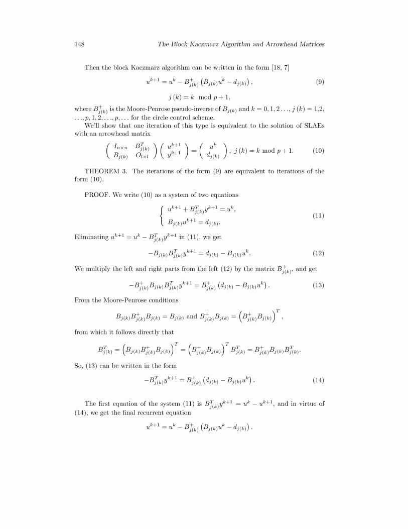
Then the block Kaczmarz algorithm can be written in the form [18, 7]

uk+1 = uk −B+j(k)(Bj(k)u

k − dj(k)), (9)

j (k) = k mod p+ 1,

where B+j(k) is the Moore-Penrose pseudo-inverse of Bj(k) and k = 0, 1, 2 . . ., j (k) = 1,2,. . ., p, 1, 2, . . ., p, . . . for the circle control scheme.We’ll show that one iteration of this type is equivalent to the solution of SLAEs

with an arrowhead matrix(In×n BTj(k)Bj(k) Ol×l

)(uk+1

yk+1

)=

(uk

dj(k)

), j (k) = k mod p+ 1. (10)

THEOREM 3. The iterations of the form (9) are equivalent to iterations of theform (10).

PROOF. We write (10) as a system of two equations{uk+1 +BTj(k)y

k+1 = uk,

Bj(k)uk+1 = dj(k).

(11)

Eliminating uk+1 = uk −BTj(k)yk+1 in (11), we get

−Bj(k)BTj(k)yk+1 = dj(k) −Bj(k)uk. (12)

We multiply the left and right parts from the left (12) by the matrix B+j(k), and get

−B+j(k)Bj(k)BTj(k)y

k+1 = B+j(k)(dj(k) −Bj(k)uk

). (13)

From the Moore-Penrose conditions

Bj(k)B+j(k)Bj(k) = Bj(k) and B

+j(k)Bj(k) =

(B+j(k)Bj(k)

)T,

from which it follows directly that

BTj(k) =(Bj(k)B

+j(k)Bj(k)

)T=(B+j(k)Bj(k)

)TBTj(k) = B+j(k)Bj(k)B

Tj(k).

So, (13) can be written in the form

−BTj(k)yk+1 = B+j(k)(dj(k) −Bj(k)uk

). (14)

The first equation of the system (11) is BTj(k)yk+1 = uk − uk+1, and in virtue of

(14), we get the final recurrent equation

uk+1 = uk −B+j(k)(Bj(k)u

k − dj(k)).


Our proof is obvious enough. Note that the representation (10) was given in [13] forthe case when the dimension of the block l = 1.

Consider the matrix of the system (10)

Bk =

(In×n BTkBk Ol×l

),

for which, for example [14], the spectral condition number is

k2

(Bk

)=

12 +

√14 + σ2max (Bk)

− 12 +√

14 + σ2min (Bk)

.

It should be noted that for small values of the condition number k2(Bk

), it may be

advantageous to use iterative methods, for example [8], to solve the system (10).

5 Proposed Algorithm

For solving SLAEs (10) at each iteration it is proposed to use the direct projectionmethod. Consider the first n of iterations of the direct projection method for solving(10):

uk+1i+1 = uk+1i + Pj(k)i ei+1

(uk (i+ 1)− uk+1i (i+ 1)− bTj(k),i+1yk+1i

)(δj(k)i+1

)−1, (15)

where i = 0, 1, . . . , n − 1, bTj(k),i+1 is the transposed i + 1th column of Bj(k), and

uk (i+ 1) is the i+1th component of the vector uk. Please note that in this section, weuse the i-index as a counter for the direct projection algorithm iterations and k-indexas a counter for Kaczmarz steps.

THEOREM 4. Suppose that the components of the vector of the initial approxi-mation satisfy the condition of consistency

uk+10 = uk −BTj(k)yk+10 , (16)

thenuk+1i+1 ≡ u

k+1i , i = 0, 1, . . . , n− 1.

PROOF. The proof of this theorem is omitted in this article: it may be easilycarried out, for example, by the method of mathematical induction.

It should be noted that a similar trick was also used in the context of the total leastsquare problem, for more, see in [23]. As a result, when the matching conditions (16)are fulfilled, the first n iterations of the direct projection method for solving (10) can


be omitted. From (7) and the fact that the main minor of the matrix of the system(10) of order n is the identity matrix, one has

Pn =

(On×n −BTj(k)Ol×n Il×l

).

Consider the ith iteration of the projection method (i = n, n + 1, . . . , n + l − 1).Then

uk+1i+1 = uk+1i + Pj(k)i ei+1

(dj(k) (i+ 1− n)− aT(j(k)−1)·l+i−n+1uk+1i

)(δj(k)i+1

)−1. (17)

Noting that the first n iterations are redundant, we introduce a new iteration numberingof the direct projection method:

ω = i− n = 0, 1, . . . , l − 1, i = n, n+ 1, . . . , n+ l − 1.

Then the direct projection method for the solution of (10) is

uk+10 = uk, yk+10 = θl, P0 =

(On×n −BTj(k)Ol×n Il×l

),

δj(k)ω+1 =

(aT(j(k)−1)·l+ω+1 θTl

)Pωen+ω+1,

uk+1ω+1 = uk+1ω + P j(k)ω en+ω+1dj(k) (ω + 1)− aT(j(k)−1)·l+ω+1uk+1ω

(δj(k)ω+1

)−1,

Pω+1 = Pω − Pωen+ω+1(aT(j(k)−1)·l+ω+1 θTl

)Pω

(δj(k)ω+1

)−1, (18)

ω = 0, 1, . . . , l − 1.

Upon completion of the iteration of the direct projection method, one needs to putuk+1l = uk+1.

The complexity of the solution of (10), taking into account the special structure ofthe matrix Pi, can be estimated as O

(16 l3 + n2l

), where l is the number of rows in the

block Bi ∈ Rl×n, i = 1, 2, . . . , p.

6 Limitations of the Proposed Algorithm

The algorithm, in theory, was proposed for only consistent and overdetermined sys-tems. But in practice, this algorithm could apply for solving inconsistent systems also,especially in the randomized form. If we want to solve underdetermined systems wecan apply the pre-conversion to the regularized augmented system (3) with the smallvalue of the regularization parameter, for more, see in [24].


7 Numerical Example

Consider the matrix Bk = {ai,j} ∈ Rl×n, where ai,j ∼ U(−√

3n ,√

3n

)has a continuous

uniform distribution on the segment[−√

3n ,√

3n

], and E (ai,j) = 0, E

(a2i,j)

= 1n ,

l ≤ n, rank (Bk) = l, E∥∥∥aT(k−1)·l+1∥∥∥ = 1,

k = 1, 2, . . . p, i = (k − 1) l + 1, (k − 1) l + 2, . . . , (k − 1) l + l and j = 1, 2, . . . n.

Notice that the condition l ≤ n is used only for this particular task, and in general itis not a limitation of the proposed algorithm. Then consider the matrix A ∈ Rm×n,whose block rows are Bk ∈ Rl×n, k = 1, 2, . . . , p, m = l · p, as in (8), and which satisfythe above mentioned conditions. In [3] (see the limit conditions of its Theorem 2),estimates are made for the minimum and maximum eigenvalues of Sk = BkB

Tk

limλmin (Sk) =

(1−

√l

n

)2, limλmax (Sk) =

(1 +

√l

n

)2. (19)

Figure 1: Black points: on the abscissa axis is(

1−√

ln

)2, on the ordinate axis

is(

1 +√

ln

)2. Gray points: on the abscissa axis is λmin (Sk), on the ordinate

axis is λmax (Sk). The figure has been plotted for all values n = 10, 11, . . . , 400 andl = 10, 11, . . . n.


We give Fig. 1 as an illustration of these limit equations.Considering (19), an ap-proximate estimate is ‖A‖2 ≈ 1 +

√mn and

σ2min (Bk) ≈(

1−√l

n

)2, σ2max (Bk) ≈

(1 +

√l

n

)2. (20)

Figure 2: Dependence of log10∥∥u∗ − uk∥∥2 from the iteration number k (on the abscissa

axis) for 100 realizations. The dotted black line shows the error estimate based on (21).The dotted white line shows the exact error based on [2].

Right-hand side vector of the test system of equations can be built by any methodensuring the consistency of the system, for example, if

f = Au∗, where u∗ = (u1, u2, . . . , un)

such as ‖u∗‖2 = 1. As a stopping criterion for the iterative algorithm, we will use therule

∥∥u∗ − uKstop∥∥2 ≤ 10−q, where Kstop is a stopping number. Note that the estimate

of the convergence rate that is used for a system of this type is referred at [15], andtake into consideration that the authors treat a consistent system of linear algebraicequations, and the initial approximation u0 = θ

E∥∥u∗ − uk∥∥2 ≤ (1− σ2min (A)

βp

)k‖u∗‖2 , (21)

where max{σ2max (Bj)

}pj=1≤ β, and the selection of the block in each iteration is


determined randomly: P (j (k) = i) = 1p , i = 1, 2, . . . , p. It follows that

Kstop =−q − log10 ‖u∗‖

2

log10

(1− σ2min(A)

βp

) . (22)

A software implementation of these numerical simulations is presented in [11]. Thelogarithm of the error versus the iteration number is plotted for p = 182 in Fig. 2, fromwhich the pessimistic estimate (21) is obvious for this problem.

Conclusion

Analyzing the results of the numerical experiment in Table 1, it should be noted thatthe optimal number of blocks for the research task, in terms of the total time of thealgorithm, is p = 182. As noted above, the complexity of each iteration of the proposed

l 1 2 4 7 8 13 · · · 364Kstop 109032 57020 30247 16244 13980 8750 · · · 118β 1.09 1.13 1.18 1.24 1.26 1.34 · · · 3.4

Kstop 368952 190996 100204 60298 98015 34977 · · · 3149p 728 364 182 104 91 56 · · · 2

Time 11.0 8.95 8.88 9.46 9.31 11.23 · · · 54.8

Table 1: Results averaged over 100 realizations of the numerical example for m = 728and n = 512, where Time is the average time of the algorithm in seconds until reachingthe prescribed accuracy when q = 8. The equation (20) was used to estimate theparameter β.

algorithm is estimated as O(16 l3 + n2l

), from which it can be concluded that it is

appropriate to choose p = ml such that l < n. In this way, we maintain a quadratic

growth of the complexity of the calculations per iteration. It is important to note thatthe system of linear equations with the same matrix Bj(k) and various right-hand partsis solved at each iteration, therefore, it is necessary to carry out a direct computationof Pω only once for each matrix Bj(k), and they can then be saved in memory forreuse. This trick will significantly reduce the number of arithmetic operations in eachiteration, but the requirements for RAM space will increase substantially.In the present paper, one iteration of Kaczmarz’s block algorithm has been presented

for the task of solving a system of linear equations with a special arrowhead matrix.But not only a direct projection method can be employed to solve such a system, socan, for example, Huang’s algorithm [1]. The particular interest for computationalmathematics is the use of a direct projection method for solving linear systems withan arrowhead matrix.

Remarks. According to the numerical experiment, the obtained estimate of thenumber of iterations before stopping, using the expression (22), is too pessimistic; in[2], the authors note this fact and offer an accurate estimate for E

∥∥u∗ − uk∥∥2. It would


be extremely useful to generalize the results of [2] to the block randomized algorithm:in this case, it is analytically possible to obtain the optimum value for p using theestimate of the algorithmic complexity.The developed algorithm in its randomized modification, as in [16], taking into

account the results of [15, 20], can be applied also to the inconsistent case.It should be noted that the direct projection method may have an effective imple-

mentation for solutions of augmented systems of the form (1), (2), and (3). Just toshow the trick for each of these systems, that is used in this paper (see the Theorem 4).The trick allow us to accept that one part of the augmented system is redundant. Itcan be the object of further research, particularly in the context of a direct projectionmethod with pivoting.

Acknowledgment. Our special thanks to Prof. G. A. Kalyabin for English proof-reading and editing.

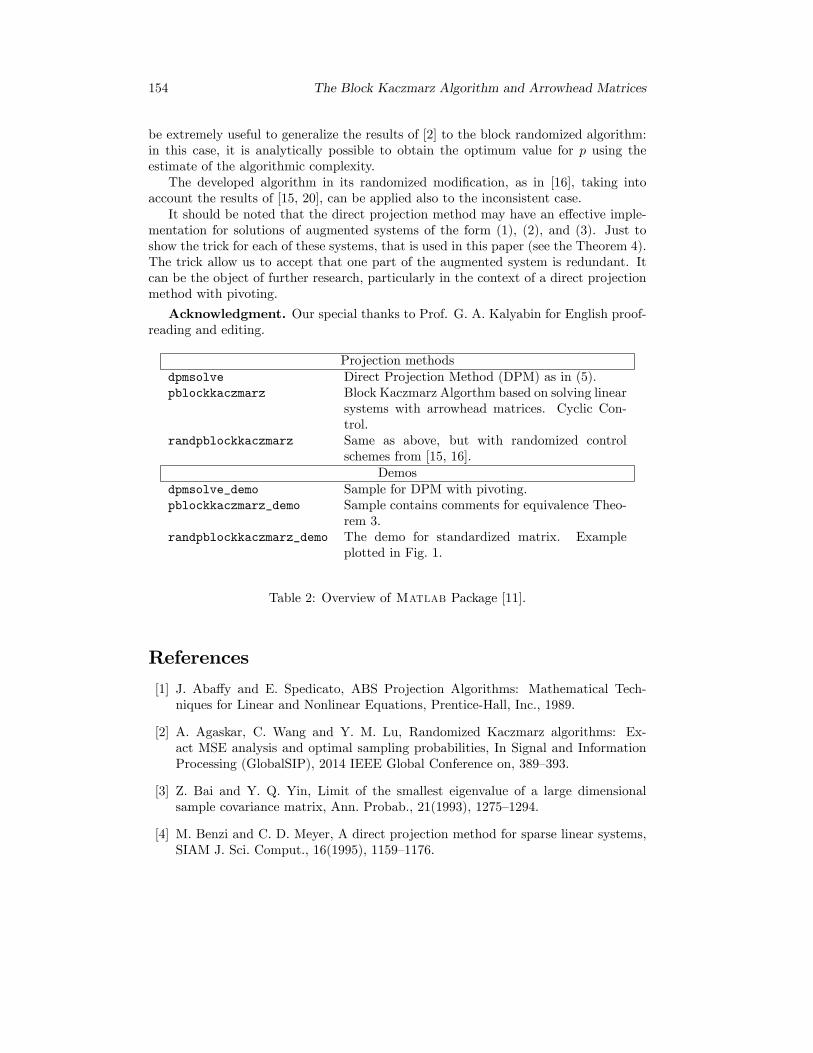
Projection methodsdpmsolve Direct Projection Method (DPM) as in (5).pblockkaczmarz Block Kaczmarz Algorthm based on solving linear

systems with arrowhead matrices. Cyclic Con-trol.

randpblockkaczmarz Same as above, but with randomized controlschemes from [15, 16].

Demosdpmsolve_demo Sample for DPM with pivoting.pblockkaczmarz_demo Sample contains comments for equivalence Theo-

rem 3.randpblockkaczmarz_demo The demo for standardized matrix. Example

plotted in Fig. 1.

Table 2: Overview of Matlab Package [11].

References

[1] J. Abaffy and E. Spedicato, ABS Projection Algorithms: Mathematical Tech-niques for Linear and Nonlinear Equations, Prentice-Hall, Inc., 1989.

[2] A. Agaskar, C. Wang and Y. M. Lu, Randomized Kaczmarz algorithms: Ex-act MSE analysis and optimal sampling probabilities, In Signal and InformationProcessing (GlobalSIP), 2014 IEEE Global Conference on, 389—393.

[3] Z. Bai and Y. Q. Yin, Limit of the smallest eigenvalue of a large dimensionalsample covariance matrix, Ann. Probab., 21(1993), 1275—1294.

[4] M. Benzi and C. D. Meyer, A direct projection method for sparse linear systems,SIAM J. Sci. Comput., 16(1995), 1159—1176.


[5] A. Björck, Numerical methods for least squares problems. Society for Industrialand Applied Mathematics (SIAM), Philadelphia, PA, 1996. xviii+408 pp.

[6] I. S. Duff and J. K. Reid, A comparison of some methods for the solution ofsparse overdetermined systems of linear equations, IMA J. Appl. Math., 17(1976),267—280.

[7] T. Elfving, Block-iterative methods for consistent and inconsistent linear equa-tions, Numer. Math., 35(1980), 1—12.

[8] G. H. Golub, X. Wu and J. Y. Yuan, SOR-like methods for augmented systems,BIT, 41(2001), 71—85.

[9] G. H. Golub and C. F. Van Loan, Matrix Computations (Vol. 3), JHU Press, 2012.

[10] A. A. Ivanov and A.I. Zhdanov, Kaczmarz algorithm for Tikhonov regularizationproblem, Appl. Math. E-Notes, 13(2013), 270—276.

[11] A. A. Ivanov, Regularization Kaczmarz Tools Ver-sion 1.4 for Matlab, Matlabcentral Fileexchange, URL:http://www.mathworks.com/matlabcentral/fileexchange/43791.

[12] S. Kaczmarz, Angenäherte auflösung von systemen linearer gleichungen, BulletinInternational de l’Academie Polonaise des Sciences et des Lettres, 35(1937), 355—357.

[13] A. Kushnerov, A seminumerical transient analysis of switched capacitor converters,IEEE Journal of Emerging and Selected Topics in Power Electronics, 2(2014), 814—820.

[14] A. Nicola and C. Popa, Kaczmarz extended versus augmented system solution inimage reconstruction, ROMAI J, 6(2010), 145—152.

[15] D. Needell and J. A. Tropp., Paved with good intentions: Analysis of a randomizedblock Kaczmarz method, Linear Algebra Appl., 441(2014), 199—221.

[16] T. Strohmer and R. Vershynin, A randomized Kaczmarz algorithm with exponen-tial convergence, J. Fourier Anal. Appl., 15(2009), 262—278.

[17] K. Sabelfeld and N. Loshchina, Stochastic iterative projection methods for largelinear systems, Monte Carlo Methods Appl., 16(2010), 343—359.

[18] G. P. Vasil’chenko and A. A. Svetlakov, A projection algorithm for solving systemsof linear algebraic equations of high dimensionality, Comput. Math. Math. Phys.,20(1980), 1—8.

[19] S. A. Vavasis, Stable numerical algorithms for equilibrium systems, SIAM J. Ma-trix Anal. Appl., 15(1994), 1108—1131.

[20] C. Wang, A. Agaskar and Y. M. Lu, Randomized Kaczmarz Algorithm for Incon-sistent Linear Systems: An Exact MSE Analysis, arXiv preprint arXiv:1502.00190(2015).


[21] X. Yu, N. K. Loh and W.C. Miller, New recursive algorithm for solving linearalgebraic equations, Electronics Letters, 28(1992), 2069—2071.

[22] A. I. Zhdanov, Direct sequence method for solving systems of linear algebraicequations, Proceedings of the Russian Academy of Sciences, 356(1997), 442—444.

[23] A. I. Zhdanov and P. A. Shamarov, A Direct Projection Method in the Problemof Complete Least Squares, Automation and Remote Control C/C of Avtomatikai Telemekhanika, 61(2000), 610—620.

[24] A. I. Zhdanov, The method of augmented regularized normal equations, Comput.Math. Math. Phys., 52(2012), 194—197.

the block kaczmarz algorithm based on solving linear

Documents