The bull and bear market model of Huang and Day:

Some extensions and new results

Fabio Tramontana, Frank Westerhoff and Laura Gardini

Working Paper No. 89

November 2012

k*

b

0 k

BA

MAMBERG

CONOMIC

ESEARCH

ROUP

BE

RG

Working Paper SeriesBERG

Bamberg Economic Research Group Bamberg University Feldkirchenstraße 21 D-96052 Bamberg

Telefax: (0951) 863 5547 Telephone: (0951) 863 2687

felix.stuebben@uni-bamberg.de http://www.uni-bamberg.de/vwl/forschung/berg/

ISBN 978-3-943153-03-3

Redaktion: Dr. Felix Stübben

felix.stuebben@uni-bamberg.de

The bull and bear market model of Huang andDay: Some extensions and new results

Fabio Tramontana1

Department of Economics and Management,

University of Pavia (Italy)

Frank Westerhoff

Department of Economics,

University of Bamberg (Germany)

Laura Gardini

Department of Economics, Society, Politics,

University of Urbino (Italy)

e-mail: fabio.tramontana@unipv.it, frank.westerhoff@uni-bamberg.de,

laura.gardini@uniurb.it

Abstract.

We develop a financial market model with interacting chartists and funda-

mentalists that embeds the famous bull and bear market model of Huang and

Day as a special case. Their model is given by a one-dimensional continuous

piecewise-linear map. Our model, on the other hand, is more flexible and is

represented by a one-dimensional discontinuous piecewise-linear map. Never-

theless, we are able to provide a more or less complete analytical treatment

of the model dynamics by characterizing its possible outcomes in parameter

space. In addition, we show that quite different scenarios can trigger real-world

phenomena such as bull and bear market dynamics and excess volatility.

Keywords: Heterogeneous interacting agents, Bull and bear market dy-

namics; Piecewise-linear maps; Border collision bifurcations.

1 Introduction

The development and analysis of financial market models with heterogeneous

interacting agents began with the seminal paper by Day and Huang (1990)2.

Based on a few stylized institutional and behavioral facts, Day and Huang pro-

posed a simple financial market model with three types of agent: a market

maker who adjusts prices with respect to excess demand; chartists who believe

in the persistence of bull and bear markets; and fundamentalists who bet on

mean reversion. In their model, market participants’ transactions may cause

apparently unpredictable price dynamics with randomly alternating periods of

1Corresponding Author. Via S.Felice 5, 27100 Pavia (PV), Italy. Tel. +39 0382-986224.2As usual, there are a number of predecessors, e.g. Zeeman (1974), Beja and Goldman

(1980), and Frankel and Froot (1986).

1

generally rising or generally falling prices, so-called bull and bear market dy-

namics. Since then, literally hundreds of follow-up papers have been presented,

deepening our understanding of how financial markets function. For surveys of

this burgeoning research field see, for instance, Chiarella et al. (2009), Hommes

and Wagener (2009), Lux (2009), and Westerhoff (2009).

The one-dimensional map studied in Day and Huang (1990) is nonlinear since

fundamentalists become increasingly aggressive as the price runs away from its

fundamental value. Huang and Day (1993) reformulated their original model

such that it corresponds to a one-dimensional continuous piecewise-linear map

by assuming that fundamentalists only start trading if the distance between the

price and its fundamental value exceeds a critical threshold value. Otherwise,

speculators’ trading strategies are linear and thus the model is represented by

three connected linear branches. Of course, simplifying assumptions must be

made to derive such a piecewise-linear map. Due to the model’s piecewise-

linearity, however, Huang and Day (1993) were able to study how certain model

parameters, e.g. chartists’ and fundamentalists’ reaction parameters, affect the

distribution of prices. They found, for instance, that an increase in funda-

mentalists’ aggressiveness tends to fatten the tails of the distribution of prices.

Obviously, such insights are quite important for our understanding of financial

markets.

In addition, the simplified model of Huang and Day (1993) initiated a sub-

stantial number of studies, some of which are described below. For instance, Gu

(1993) managed to estimate the model of Huang and Day (1993) on the basis of

monthly S&P 500 data, and discovered that the distribution of model-generated

price changes does not differ statistically from its empirical counterpart. In addi-

tion, the autocorrelation functions of simulated and actual returns are strikingly

similar. Gu concludes that although random elements play a role in the price

formation process, the majority of the dynamics is due to intrinsic market forces,

as represented by the simple model of Huang and Day (1993), for instance.

Gu (1995) further extended the analysis of Huang and Day (1993) by deriving

closed form density functions of prices. In particular, he used this result to study

how aggressively the market maker has to adjust prices with respect to excess

demand to make profits (density functions depend on market maker’s price

adjustment behavior and control her/his profits). Gu showed that the market

maker has to churn the market to make a living. Although it is undesirable for

the market maker to destabilize the market too considerably, she/he evidently

has an incentive to keep prices moving. Gu, too, admitted that the underlying

piecewise-linear model is based on simplifying assumptions. Again, however,

these assumptions enabled rigorous results to be derived that have real practical

relevance.

In reality, of course, there are more than two different types of speculator.

Speculators may differ with respect to degree of aggressiveness, their trading

horizons, market entry levels, perceptions of the fundamental value, and so on.

Day (1997) thus considered the case where there are different types of funda-

mental and technical traders, and presented an example of a one-dimensional

continuous piecewise-linear map with 11 branches. As it turns out, this model is

2

capable of generating quite exciting dynamics. For instance, bull and bear mar-

kets may emerge at quite different levels and the price dynamics may become

even more intricate.

Tramontana et al. (2010a) developed a model in which chartists and fun-

damentalists react asymmetrically to bull and bear market situations. For in-

stance, market participants may trade more/less aggressively in overvalued mar-

kets than in undervalued markets. As a result, they obtain a one-dimensional

discontinuous piecewise-linear map (where the discontinuity point is given by

the market’s fundamental value). Although the mathematical tools for study-

ing such models continue to be underdeveloped, they offer a detailed analytical

treatment of the underlying map, which can produce all kinds of dynamic be-

havior including fixed point dynamics, cycles, quasi-periodic motion, chaos, and

exploding trajectories. This model was further developed and investigated in

Tramontana et al. (2010b, 2011). Besides identifying economic mechanisms

that can produce endogenous bull and bear market dynamics, these papers

enrich our knowledge about how to deal with one-dimensional discontinuous

piecewise-linear maps3.

Huang and Zheng (2012) also presented a model in the spirit of Huang and

Day (1993) to explain different types of financial crisis, in particular, the sudden

crisis, the disturbing crisis, and the smooth crisis. In their model, chartists hold

regime-dependent beliefs about the fundamental value, motivated by psycho-

logically grounded support and resistance levels; the different types of crisis are

explained by a constant switching between regimes. In addition, their model

is also able to explain a number of stylized facts concerning financial markets.

The underlying map is essentially represented by a one-dimensional discontinu-

ous piecewise-linear map where all branches have a positive slope. Huang et al.

(2010) modified the latter model by allowing traders to switch between technical

and fundamental trading strategies according to an evolutionary fitness measure.

On the basis of this model, Huang et al. (2012) demonstrated, amongst other

things, that major stock market movements and returns are asymmetric, i.e.

that bubbles emerge gradually and crash suddenly and that drawdowns tend to

be more dramatic than drawups.

Another model inspired by Huang and Day (1993) is that by Venier (2008).

Despite its deterministic nature, his model, represented by a saw-tooth map,

was able to reproduce some stylized facts concerning financial markets, such

as fat tails and volatility clustering. By buffeting their one-dimensional dis-

continuous piecewise-linear bull and bear market model with dynamic noise,

Tramontana and Westerhoff (2013) obtained a good match of the statistical

properties of actual financial market prices, also from a quantitative perspec-

tive. Westerhoff and Franke (2012) provided an even simpler but nonetheless

powerful stochastic bull and bear market approach. Further empirical evidence

for regime-dependent trading behavior of chartists and fundamentalists is pro-

3The formal analysis of one-dimensional discontinuous piecewise-linear models with one

discontinuity can be traced back to Leonov (1959, 1962). Recently, this research field has

gained new momentum; see, for instance, Gardini et al. (2010), Avrutin et al. (2010), Gardini

and Tramontana (2010).

3

vided by Chiarella et al. (2012), Manzan and Westerhoff (2007), and Vigfusson

(1997), amongst others.

To sum up, simple piecewise-linear models enable us to derive new analytical

insights into how financial markets function. Moreover, these models — despite

their simplicity — are not at odds with reality. Firstly, their main building

blocks are based on stylized institutional and behavioral facts. For instance, the

survey study conducted by Menkhoff and Taylor (2007) revealed that market

participants do indeed rely on technical and fundamental analysis to predict

financial market prices (this has also been found in laboratory experiments; see,

e.g. Hommes 2011). Secondly, these models are able to explain some important

stylized facts concerning financial markets such as bubbles and crashes, excess

volatility, and long-memory effects. Given the repeated emergence of severe

financial crises and the associated risk to the real economy, we believe that

more work should be undertaken in this exciting research direction.

In this paper, we thus continue this line of research by proposing a financial

market model that may be regarded as a generalization of the model of Huang

and Day (1993). Let us briefly recall why their one-dimensional piecewise-

linear map is continuous. Close to the fundamental value, only chartists are

active in the market. Hence, the slope of the map’s inner branch is larger

than one. If the price deviates too far from the fundamental value, additional

fundamentalists enter the market. Since their demand is zero when they enter

the market, all three branches of the map are connected, and the slope of the

two outer branches is lower than the slope of the inner branch. Instead, we

assume that a number of chartists and fundamentalists are always active in the

market, that additional chartists and additional fundamentalists may enter the

market when the distance between the price and its fundamental value exceeds

a critical level, and that new traders’demand may be non-zero at the market

entry level. As a result, the dynamics of our model is due to a quite flexible

one-dimensional discontinuous piecewise linear map. In particular, the three

branches are typically disconnected, and there are no restrictions to the values

their slopes may assume.

Nevertheless, we are able to provide a comprehensive analysis of the model

dynamics. For instance, we are able to determine the frontiers, in parameter

space, that separate bounded dynamics from divergent dynamics. This analysis

demonstrates that both chartists and fundamentalists can contribute to or pre-

vent market stability, making the regulation of financial markets a delicate issue.

Moreover, we find that quite different scenarios can lead to intricate bull and

bear market dynamics. As in Huang and Day (1993), we observe repeated price

rallies and subsequent market crashes if the slope of the two outer branches is

negative, due to fundamentalists’ aggressive trading behavior. However, we also

observe such — and even more intricate — boom-bust dynamics if the slope of

the two outer branches is positive, due to chartists’ aggressive trading behavior.

Overall, the emergence of endogenous bull and bear market dynamics may thus

be regarded as a robust and characteristic feature of speculative markets.

Our model results in a discontinuous map with two discontinuity points.

Exploration of the so-called border collision bifurcations that occur in this case

4

is in its infancy. A few results can be found in Tramontana et al. (2012c), in

which, however, only stable regimes are investigated (i.e. the slopes of all three

branches are between 0 and 1). Clearly, such a scenario does not occur in our

model. Thus, from a mathematical point of view, our model reveals exciting

dynamics and interesting bifurcation structures, some of which have never yet

been documented in the literature. As we will see, our analysis will also highlight

a number of open problems, presenting non-trivial (mathematical) challenges for

future research. We also hope that the detailed formal analysis of our model

will help other researchers to explore their own discontinuous piecewise-linear

maps. Unfortunately, as already noted, our knowledge about such maps is as yet

rather limited. Variations of our model (still with two discontinuity points) are

studied in Tramontana et al. (2012a) and Tramontana et al. (2012b). However,

these models do not embed the model of Huang and Day (1993) as a special

case.

The remainder of our paper is organized as follows. In Section 2, we present

our financial market model and show that it corresponds to a one-dimensional

discontinuous piecewise-linear map. In Section 3, we give an overview of the

potential model dynamics and illustrate its economic implications. Section 4 has

a stronger mathematical orientation and explores some interesting parameter

regions in further detail. In Section 5, we conclude the paper and highlight

avenues for further research.

2 A simple financial market model

Our model is closely related to those of Day and Huang (1990) and Huang

and Day (1993), and may even be interpreted as a generalization of the latter.

Following the original papers, we assume that a market maker adjusts prices

with respect to excess demand in the usual way. In our case, excess demand

comprises the transactions of four different types of market participant. So-

called type 1 chartists and type 1 fundamentalists are always active in the

market. Type 1 chartists bet on the persistence of bull and bear markets while

type 1 fundamentalists expect the price to return to its fundamental value.

So-called type 2 chartists and type 2 fundamentalists share the same general

trading philosophy as their type 1 counterparts, but only enter the market if

mispricing exceeds a critical threshold value. Huang and Day (1993) argue that

fundamentalists may perceive the chance of gains as small or zero near to the

fundamental value and thus may opt against the participation in the trading

process. For chartists, it can be argued that they only learn about (or trust)

bull and bear markets if mispricing is sufficiently extreme. Of course, these

are simplifying assumptions. Nonetheless, it appears natural to us to assume

that not all traders react immediately to their trading signals. We will now

present the building blocks of our model and show that they constitute a one-

dimensional discontinuous piecewise-linear map.

5

2.1 The setup

Within our model, the price formation is due to a (standard) log-linear price

adjustment rule according to which excess buying drives prices up and excess

selling drives them down. Such a rule may also be interpreted as the stylized

price setting behavior of a risk-neutral market maker. Let be the log of the

price. Then we have

+1 = + ³1 +

1 +

2 +

2

´ (1)

The four terms in brackets on the right-hand side of (1) capture the transactions

conducted by type 1 chartists, type 1 fundamentalists, type 2 chartists, and

type 2 fundamentalists, respectively. Parameter is a positive price adjustment

parameter which we set, without loss of generality, equal to = 1.

Type 1 chartists optimistically buy (pessimistically sell) if prices are in the

bull (bear) market, that is, if log price is above (below) its log fundamental

value . Their orders are formalized as

1 = 1 ( − ) (2)

Reaction parameter 1 is positive and indicates how aggressively type 1 chartists

react to their perceived price signals. The larger 1 is, the more aggressive type

1 chartists are.

Type 1 fundamentalists always trade in the opposite direction of type 1

chartists. Orders placed by type 1 fundamentalists are written as

1 = 1 ( − ) (3)

where reaction parameter 1 is positive. In an overvalued market, therefore,

type 1 fundamentalists sell; in an undervalued market they buy.

Type 2 speculators are only active if prices are at least a certain distance from

their fundamental value. The critical distance for type 2 speculators is given by

, a positive constant4. The orders of type 2 chartists are thus expressed as

2 =

⎧⎨⎩ 2 ( − ) + 3 for − ≥

0 for − −

2 ( − )− 3 for − ≤ − (4)

Again, reaction parameter 2 is positive, i.e. the trading intensity of type 2

chartists increases in line with the distance between prices and fundamentals.

However, their transactions can be adjusted using parameter 3 for which we

assume 3 ≥ −2( − ). Therefore, type 2 chartists’ transactions are non-

negative in the bull market and non-positive in the bear market.

4Here we assume that different market entry levels for type 2 chartists and type 2 fun-

damentalists would result in a one-dimensional discontinuous piecewise linear map with 4

discontinuity points and 5 branches. We leave this mathematically intricate scenario for the

future. However, it should be noted that many cases discussed in this paper are consistent

with a model where there are either only type 2 chartists or only type 2 fundamentalists.

6

Orders placed by type 2 fundamentalists are based on the same principles,

i.e. we have

2 =

⎧⎨⎩ 2 ( − )− 3 for − ≥

0 for − −

2 ( − ) + 3 for − ≤ − (5)

where restrictions 2 0 and 3 ≥ 2( − ) hold.

2.2 The model’s law of motion

To simplify the notation, let us define

1 = 1 − 1 2 = 2 − 2 and = 3 − 3

Note first that there are no restrictions on these aggregate parameters (they can

take any values). Combining (1) to (5) then yields

+1 =

⎧⎨⎩ + (1 + 2) ( − ) + if − ≥

+ 1 ( − ) if − −

+ (1 + 2) ( − )− if − ≤ −

(6)

Furthermore, it is convenient to express the model in terms of deviations from

the fundamental value by defining e = − . We then have

e+1 =⎧⎪⎨⎪⎩(1 + 1 + 2) e + if e ≥

(1 + 1) e if − e

(1 + 1 + 2) e − if e ≤ − (7)

i.e. prices are driven by a one-dimensional piecewise linear map that has three

separate linear branches.

Note that this map embeds the famous models of Day and Huang (1990)

and, in particular, Huang and Day (1993) as special cases. We obtain their

model if we assume that 1 = 0, i.e. there are no type 1 fundamentalists;

2 = 3 = 0, i.e. there are no type 2 chartists; and 3 = 2( − ), i.e. type 2

fundamentalists’ demand is zero at the market entry level. In this case, the two

outer branches are connected with the inner branch. The inner branch has a

slope that is always larger than one. However, interesting bull and bear market

dynamics only occurs in their model if the slope of the two outer branches is less

than minus one. Note that the latter condition requires that fundamentalists

trade quite aggressively. Our model is more flexible by imposing less restrictive

assumptions on traders’ behavior. In general, the slopes of its outer and inner

branches can be positive or negative, and the map is discontinuous. As we will

show in the next section, this leads to quite interesting bifurcation properties

and new bull and bear market scenarios.

7

3 Dynamics of the model: a first overview

In this section, we present an overview of the model dynamics. In Section 4, we

will proceed to study certain aspects of the model dynamics in further detail.

Following Huang and Day (1993), we assume from here on that (1 + 1) 1.

Economically, this implies that type 1 chartists react more aggressively to a

given price signal than type 1 fundamentalists (i.e. 1 1 and thus 1 0)5 .

Apart from this assumption, both and (1 + 1 + 2) can take any positive

or negative value, and 0.

Note first that market entry level can be considered as a scale variable.

By using the change of variable = e and by setting =, we obtain:

: 0 =

⎧⎨⎩ () = (1 + 1 + 2)+ if 1

() = (1 + 1) if −1 1

() = (1 + 1 + 2)− if −1 (8)

where "0" denotes the unit time advancement operator.One useful property of the model is that its dynamics is symmetric with

respect to the origin = 0. Using the definition = − results in

0 =

⎧⎨⎩ (1 + 1 + 2) + if 1

(1 + 1) if −1 1

(1 + 1 + 2) − if −1 (9)

which is identical to in (8), meaning that the following property holds6:

Property 1 (Symmetry). Any invariant set of the map in (8) is either

symmetric with respect to = 0 or the symmetric set also exists.

A direct consequence of Property 1 is that cycles of odd periods are never

unique since the symmetric cycle also exists. That is, if a cycle with periodic

points (1 ) exists where is odd (and whatever is the sign of , positive

or negative), then the cycle (−1 −) also necessarily exists. As we shallsee, this property will lead to a peculiar dynamic behavior described in Section

4.

In general, map is discontinuous, with two discontinuity points in = −1and = 1. In fact, map is continuous only if:

(1) = (1) (10)

With respect to the model parameters, this condition can be rewritten as:

() : 2 = − (11)

5As a result, type 1 chartists’ transactions drive the price monotonically away from the

fundamental value. Of course, for (1 + 1) −1 the inner regime also becomes unstable.Then, however, type 1 fundamentalists’ transactions cause explosive improper oscillations. A

detailed mathematical analysis of this case is quite involved and will necessitate a separate

paper.6Recall that an invariant set is a set that satisfies () = .

8

and always holds in the framework of Huang and Day (1993).

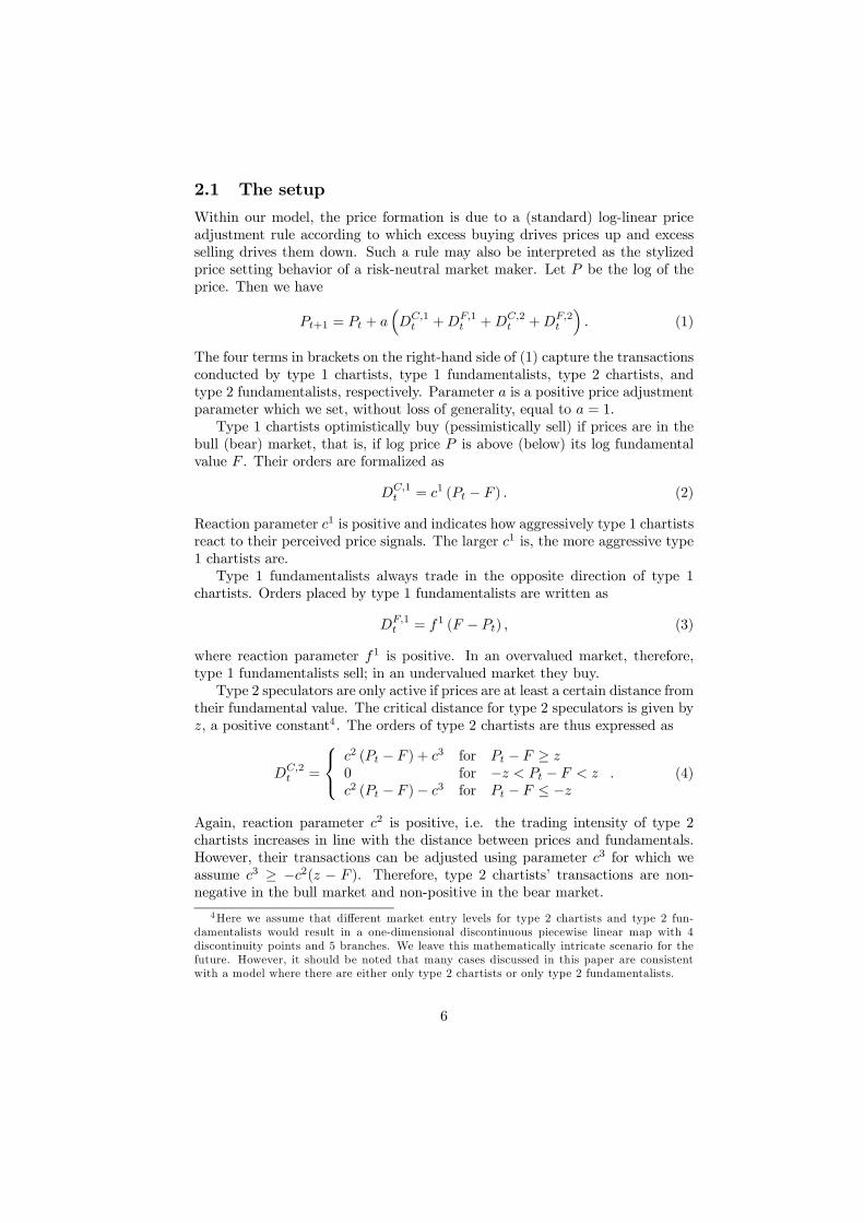
Let us next consider the two-dimensional bifurcation diagram in Fig. 1.

Here we fix 1 = 05 and vary 2 and as indicated on the axes7. The

aforementioned locus of continuity is represented by straight line (). Note

also that Huang and Day (1993) only consider a market entry of additional

fundamentalists. In their model, 2 is thus always negative. As will become

clearer below, the model of Huang and Day (1993) may produce two symmetric

stable fixed points (line (C), yellow region in Fig. 1), chaotic dynamics (line

(C), white region in Fig. 1), which can be with two disjoint chaotic intervals

(see Fig. 2a for an example) or in a unique chaotic interval (see Fig. 2b for an

example), and divergent dynamics (line (C), gray region in Fig. 1). Naturally,

our model includes a much larger parameter space and, as already visible from

Fig. 1, many different dynamic peculiarities.

Fig.1 Two-dimensional bifurcation diagram in the parameter plane (2) at

1 = 05 fixed.

Since the central branch () of map (8) is a straight line running through the

origin with a slope always greater than 1, the dynamic properties of our model

strongly depend on external branches () and (), that is on parameter

and (1 + 1 + 2). As we will see in further detail in Section 4, the parameter

regions

(1) : (1 + 1 + 2) 0 and 0;

(2) : (1 + 1 + 2) 0 and 0; (12)

(3) : (1 + 1 + 2) 0 and 0;

(4) : (1 + 1 + 2) 0 and 0;

7 In all of our simulations, we set 1 = 05. However, we obtain similar results for any

other value of 1.

9

produce quite different dynamics. In Fig. 1, we thus draw the lines = 0 and

2 = −15 (which results from (1 + 1 + 2 = 0) and 1 = 05) to mark the

four regions.

Fig. 2 In (a) = 3, 2 = −3; in (b) = 5, 2 = −5Economically, (1 + 1 + 2) 0 implies that the joint price-dependent trading

impact of type 1 and type 2 fundamentalists strongly overcompensates the joint

price-dependent trading impact of type 1 and type 2 chartists. Similarly, it may

be argued that for 0 (1+1+2) 1 the joint price-dependent trading impact

of type 1 and type 2 fundamentalists weakly overcompensates the joint price-

dependent trading impact of type 1 and type 2 chartists while for (1+1+2)

1 the joint price-dependent trading impact of type 1 and type 2 fundamentalists

is overcompensated by the joint price-dependent trading impact of type 1 and

type 2 chartists. Moreover, 0 ( 0) can be interpreted in the sense that

the price-independent trading impact of type 2 chartists is stronger (weaker)

than the price-independent trading impact of type 2 fundamentalists.

Since our map is piecewise-linear and since the slope of the central

branch is higher than 1, it follows that stable cycles can only exist in the strip

−1 (1 + 1 + 2) 1 (13)

that is

−2− 1 2 −1 (14)

This can also be seen in Fig. 1 (where 1 = 05 turns (14) into −15 2

−05).The fixed points of map (8), apart from = 0 which is always unstable,

are associated with the symmetric external branches. Solving () = and

() = leads to

∗ =

1 + 2 ∗ = −

1 + 2 (15)

Of course, the fixed points only exist if ∗ −1 and ∗ 1. For instance, for

∗ we thus have − 1+2

1 , which occurs for (a) 2 − − 1 if 0

10

and 1 + 2 0 or (b) 2 −− 1 if 0 and 1 + 2 0. Thus in Fig.

1 we also show the straight line

() : 2 = −− 1 (16)

Hence, the symmetric fixed points are stable only for 0 in the strip −2 −1 2 −1 (the yellow area in Fig. 1). As we will study in further detailbelow, in a portion of this area the fixed points coexist with a stable period

2-cycle. For 0, the fixed points, if they exist, are always unstable.

From an economic perspective, a fixed point implies that the market maker

adjusts the price no further. The reason for this is, obviously, that excess

demand is zero. For = 0, excess demand is zero since the price is equal to

its fundamental value, and thus speculators do not perceive any trading signals.

For ∗ and ∗, however, excess demand is zero since speculators’ buying andselling orders cancel each other out.

Outside the strip −2 − 1 2 −1, the dynamics is either chaotic (asall the slopes are in modulus larger than 1) or the generic trajectory explodes

(marked by white and gray in Fig. 1, respectively). As it turns out, it is pos-

sible to determine the frontiers separating bounded dynamics from the regions

of divergent trajectories analytically. Consider the case of unstable fixed points

for 0 (the qualitative shape of map is as shown in Fig. 3a).

Fig. 3 In (a) = −3, 2 = 08; in (b) = 5, 2 = −4As long as the dynamics is bounded, the unstable fixed points are on the bound-

ary of the basin of attraction:

B() =]∗

∗[ (17)

and a condition leading to a so-called final bifurcation is the homoclinic bifur-

cation of the unstable fixed points, which occurs when the offsets of the central

branch reach the fixed points, i.e. when

(1) = ∗ (18)

11

and clearly also at the same time (−1) = ∗ which leads to the condition

(1) : 2 = −

1 + 1− 1 (19)

(straight line (1) in region 0 in Fig. 1a).

However, a homoclinic bifurcation of the fixed points may also occur due to

a change in the slopes and offsets of the external branches, when the condition

(−1) = ∗ (20)

occurs, which leads to the following condition to be satisfied:

(2)2 + 2(1 + 21 +) + (1(1 + 1) +1 −) = 0 (21)

the solution of which is expressed by the two branches of equation

(2) : 2 =1

2(−(1+21+)±

p(1 + 21 +)2 − 4(1(1 + 1) +1 −)

(22)

shown as (2) in Fig. 1a.

We have to reason differently in the case 0. If the fixed points do not

exist (an example is shown in Fig. 4), then an unstable 2-cycle exists, with

periodic points and = − in the external branches of (i.e. with

symbolic sequence ), where satisfies ◦ () = . This leads to

=−

2 + 1 + 2 (23)

This unstable 2-cycle bounds the basin of attraction of the existing chaotic set:

B() =] [ (24)

and the bifurcation leading to divergent trajectories occurs at the homoclinic

bifurcation of this 2-cycle, which occurs when

(1) = (25)

This leads to the condition

(3) : 2 =−1 + 1

− 2− 1 (26)

which is the straight line (3) in Fig. 1a.

A second way to obtain the homoclinic bifurcation of the unstable 2-cycle

on the basin boundary is due to the external branches (see the qualitative shape

of the map in Fig. 3b, and the unstable fixed points are included in the chaotic

intervals). This occurs when the condition

(1) = (27)

12

is satisfied, which leads to:

(2)2 + 2(2(1 + 1) + 1 +) + (1 + 1)2 + (1 + 1)(1 +) + 2 = 0 (28)

The solution of this is expressed by the two branches of equation

(4) : 2 = 12(−(2(1 + 1) + 1 +)±p

(2(1 + 1) + 1 +)2 − 4((1 + 1)2 + (1 + 1)(1 +) + 2)

(29)

shown as (4) in Fig. 1a. Thus we have proved the following

Property 2 (divergence). For any value of , outside the region satis-

fying −2 1 + 2 0 either chaotic dynamics exist or the generic trajectory

is divergent. The region with divergent trajectories is bounded by the surfaces

given in (19) and (22) for 0, and in (26) and (29) for 0 Chaos

occurs in robust chaotic intervals of map .

Let us take a closer look at Fig. 1 and the region bounded by (d1)-(d4).

Naturally, one important goal of a central authority would be to prevent a mar-

ket from collapsing, i.e. to prevent the price trajectory from settling on an

explosive course. However, as is clear from Fig. 1, the regulation of financial

markets is a non-trivial, challenging task. Note that either an increase or de-

crease in parameter 2 and/or parameter , and thus an increase or decrease in

the aggressiveness of type 2 chartists and type 2 fundamentalists, may benefit

or harm market stability. On the other hand, we learn from Fig. 1 that markets

at least do not explode as long as the condition −2 − 1 2 −1 is met.Given our model, a central authority may thus seek to manipulate the slopes

of the outer branches of the underlying map such that they fall into this corri-

dor, for instance by following appropriate intervention strategies (e.g. Wieland

and Westerhoff 2005 studied the impact of chaos control-inspired intervention

strategies within the original model of Day and Huang 1990).

A number of examples of chaotic dynamics outside the strip −2 1+2

0 are shown in Fig. 4 for 0 and decreasing external branches, in Fig. 5 for

0 and increasing branches. As can be seen, both parameter combinations,

despite being quite different, can produce complex bull and bear market dynam-

ics, which underlines the robustness of this finding. In the following, we sketch

how these price fluctuations come about. However, let us first return to Fig. 2,

which illustrates the dynamics of the original model of Huang and Day (1993).

Suppose, for a start, that the price is slightly above the fundamental value.

Since only chartists are active in that market area, prices are driven upwards,

period for period, until fundamentalists enter the market. Since fundamentalists

trade quite aggressively, prices are pushed downwards. Fig. 2 reveals that as

long as the price drop is not too extreme, i.e. as long as the market remains in

its bull state, prices will rise again, due to chartists’ transactions. This pattern

repeats itself in a complex manner, enabling us to observe irregular bull market

dynamics. However, when prices reach a very high level, fundamentalists’ trans-

actions may become so forceful that the resulting price drop turns the market

into a bear market. From then on, the chartists’ previously optimistic mood

13

turns pessimistic, and they expect a further price decrease. And indeed, prices

decrease — until fundamentalists re-enter the market again and push prices up-

wards. We may now observe a longer bear market episode or, alternatively, a

faster comeback of a bull market. It is virtually impossible to predict the dura-

tion of bull and bear markets, which is one of the aspects that make the model

of Huang and Day so interesting.

Fig. 4 In (a) = 25, 2 = −33; in (b) versus time trajectory. Points belongingto the grey strip on the bull region are mapped in one iteration in the bear region. A

symmetric strip exists in the bear region, mapping points in the bull region in one

iteration.

Let us now take a look at Fig. 4. Essentially, the dynamics is similar to that

just discussed. In our generalized model, we also see more or less randomly al-

ternating periods of complex bull and bear market dynamics, despite the map’s

two discontinuities. Depending on the size of parameter 0, however, we

may observe larger price drops more/less frequently. Recall that in our model,

chartists and fundamentalists are always jointly active. In the inner regime,

the trading activity of type 1 chartists is stronger than that of type 1 funda-

mentalists. For this reason, the slope of the map’s inner branch is higher than

one, and prices are driven away from the fundamental value. At some point,

however, additional speculators enter the market. Depending on the relative

strength of type 2 chartists and type 2 fundamentalists, the slope and location

of the two outer branches change. The specification in Fig. 4 is such that the

aggregate transactions of all speculators produce more rapid price corrections

than observed in Huang and Day’s original model.

The situation differs in Fig. 5, where a new price pattern also emerges. What

do the parameters now imply? Note that 0 can be interpreted in the sense

that the price-independent trading behavior of type 2 fundamentalists is quite

pronounced, while 2 0 can be interpreted in the sense that type 2 chartists

trade rather aggressively on their price signals. The new feature of Fig. 5 is

as follows: observe, for instance, that a transition from a bull market to a bear

market now emerges for more intermediate price levels rather than for very high

price levels. Here we have a situation in which fundamentalists’ selling orders

14

exceed chartists’ buying orders to such an extent that the consequent price drop

triggers a bear market. If the price had been somewhat higher, however, we

would still have observed a price drop. Due to the increased number of buying

orders placed by chartists and the higher price level, however, the bull market

would have survived. Hence, our model is able to generate a different regime-

shifting pattern, and it may be argued that the price dynamics becomes even

more erratic. Other examples of complex bull and/or bear market dynamics are

depicted in Figs. 7, 8, 9, 11 and 12, further supporting the robustness of bull

and bear market dynamics.

Fig. 5 In (a) = −3, 2 = 08; in (b) versus time trajectory. Points belonging tothe gray strip in the bull region are mapped in one iteration in the bear region. A

symmetric stripe exists in the bear region, and points in this reason are mapped in

one iteration in the bull region.

Apart from the regions with chaotic dynamics outside the strip −2 1+2

0, another quite interesting region is given exactly by this strip. As we will

see, attracting cycles of any period can exist in this particular strip, and the

boundaries can also be analytically determined. In the enlargement in Fig. 1b

we illustrate the periodicity regions associated with stable cycles using different

colors. We can also see from the structure of the regions that we have different

dynamic properties in regions 0 and 0 and also, depending on the sign

of the slope (1+1+2), of the external branches, i.e. in the four regions defined

in (12), as described in the next section. First of all, however, the separating case

occurring at value = 0 deserves special mention. Recall that a very important

property of piecewise-linear maps is whether or not they are invertible. In fact,

when a piecewise-linear map is invertible inside an invariant interval (i.e. with

a unique inverse in the invariant interval), then only stable dynamics can exist,

i.e. no unstable cycle or chaotic dynamics can occur, as proved in Keener (1980).

However, when the map is non-invertible, stable and unstable cycles can exist,

as well as chaos. In our case, considering the discontinuity point on the positive

side, where the map is increasing/increasing (i.e. all slopes are positive), the

15

invertibility condition, given by

◦ (1) ◦ (1) (30)

reads as

(1 + 1) (31)

which is always satisfied in region (1). Moreover, the condition

◦ (1) = ◦ (1) (32)

is satisfied for = 0, which implies that for = 0 map is conjugated

with a circle map and, in particular, with a linear rotation, whose dynamics are

well known. That is, either all points of the absorbing interval are periodic (of

the same period) or any trajectory is quasiperiodic and dense in the absorbing

interval (see also Gardini et al. (2010), Gardini and Tramontana (2010)). This

depends on the rotation number, rational or irrational, respectively, and can also

be observed numerically: the points associated with rational rotation numbers

are the points on = 0; the periodicity regions in Fig. 1b emanate from there.

Thus we can state the following

Property 3 (linear rotation). For = 0 and −2 1 + 2 0 map

is conjugated with a linear rotation.

4 Dynamics of the model in regions R1-R4

In this section, we characterize the model dynamics in parameter regions (1)-

(4). The dynamics in regions (1) and (2) can easily be related to well-

known results of discontinuous maps with only one discontinuity point (see

Gardini et al. 2010, Avrutin et al. 2010, and Gardini and Tramontana 2010).

However, new dynamic behaviors and new bifurcation structures may occur

when all three branches of the map start to interact (although a few results

exist for maps with two discontinuity points by Tramontana et al. 2012a,b,c,

they cannot be applied in our case).

To make our mathematical analysis as stark as possible, we decided to refrain

from giving a deeper economic discussion of our results in Section 4. In doing so,

we hope that our analysis will be easier to follow and may encourage the study

of other economic models and further discontinuous piecewise-linear maps. So

far, our knowledge about such systems is, unfortunately, quite limited. In any

case, the economic meaning of parameters 1, 2 and is well defined and thus

the economic implications of our study should be straightforward to deduct.

Due to the symmetry of our map, and the useful notation in terms of sym-

bolic sequences to represent existing cycles, we shall use and to describe

the right-most and left-most branches of our map , while the central branch

is separated by the origin on the right and the left, denoted by + and −respectively.

16

4.1 Region (1): adding structure and disjoint symmetric

attractors

All the branches of map are increasing in region (1). It is clear that for

(1) 1 i.e. for 2 −− 1 (as we have seen in (16) and (15)), a stable

fixed point exists on the right, and similarly on the left. It follows that ∗attracts all initial conditions 0 0 while

∗ attracts all negative ones.

Regarding the remaining portion, in (1) and −(1 + 2), the map is

uniquely invertible in two disjoint (symmetric) absorbing intervals, one on the

positive side and one on the negative side, and without fixed points. Any initial

condition 0 0 converges to the unique attractor existing in

= [(1) (1)] = [1 + 1 + 2 + 1 + 1] (33)

and similarly in the negative one in the absorbing interval

= [(−1) (−1)] = [−(1 + 1)−(1 + 1 + 2 +)] (34)

As already noted, in this range we can take advantage of the properties of a

map with one discontinuity point. Hence we can state that all dynamics is

regular. Stable cycles of any period exist. Applying the formulas reported in

several papers (see, for example, Gardini et al. (2010)), we can also write the

explicit analytic equations of BCB curves (really surfaces in our case, since the

parameter space is three-dimensional), leading to a stable cycle in any period.

Such cycles are organized in complexity levels. As we can see from Fig. 1b,

the so-called regions of cycles of the first complexity level (or maximal cycles)

of period ( + 1) for any ≥ 1 have symbolic sequences + above the

region of the attracting 2-cycle, and symbolic sequences + below the region

of the 2-cycle. Then, between any two consecutive regions of cycles of the

first complexity level, for example between + and +

+1 we can detect

two infinite families of periodicity regions of cycles of the second complexity

level with symbolic sequence (+)+

+1 and +(+

+1) for any

≥ 1 and so on: between any two consecutive periodicity regions of cycles

of complexity level we can find two infinite families of cycles of complexity

level + 1 by using the same adding rule in the symbolic sequences. That is,

the adding mechanism leads to the structure of the attracting cycles and their

periodicity regions, as evident in Fig. 1b.

A one-dimensional bifurcation diagram showing the dynamic behavior of our

variable is illustrated in Fig. 6a for 0 at fixed parameters for 1 and

2 (along the horizontal path (A) shown in Fig. 1b). The attracting set on

the positive side is shown in black. The symmetric dynamics clearly also exists

on the negative side (shown in red in Fig. 6a). The symbolic sequence of the

orbits is obtained from those on the right, substituting + and with − and, respectively. The adding mechanism in the structure of the attracting cycles

is clearly evident in Fig. 6a. We also recall that for 0 −(1 + 2) the

intervals associated with stable cycles are dense in the interval (0−(1 + 2))

The parameter points that do not belong to the closure of a periodicity region

17

of a certain cycle are associated with stable non-periodic dynamics: the trajec-

tory ultimately converges to a non-chaotic Cantor set attractor, on which the

trajectories are quasiperiodic and dense.

Fig. 6 One-dimensional bifurcation diagram as a function of m. In (a) along path

(A) of Fig. 1b, at 2 = −12; in (b) along path (B) of Fig. 1b, at 2 = −18

4.2 Region (2): increment structure and chaotic inter-

vals

The external branches of are decreasing in the region (2). For (1) 1

i.e. for −(1 + 2) (as we have seen in (16) and (15)), a stable fixed

point may exist on the right, and similarly on the left. However, the stable

fixed point may now no longer be the unique attractor. In fact, when the fixed

points exist, the shape of the map is increasing/decreasing in the two disjoint

absorbing intervals on the two opposite sides. For such kinds of maps, with one

discontinuity only in each invariant interval, we know there exists of a regime of

bistability, and a so-called increment structure for existing cycles (see Gardini

and Tramontana, 2010). Thus we have to separate the cases in which two

disjoint absorbing intervals exist, or only a unique one. For the particular value

(1 + 1 + 2) = 0 the external branches are flat, which corresponds to the

transition between regions (1) and (2). This case is also well known: the

interval (0−(1 + 2)) = (0−1) consists of consecutive segments associatedwith one unique cycle in each absorbing interval; on the right they have the

symbolic sequence + (on the left

−) The boundary points between one

period and the other correspond to so-called big bang bifurcation points in

the parameter space (see Fig. 1b). They correspond to the intersection of

18

two different border collision bifurcation curves. Infinitely many BCB curves

are issued on one side from those points (in our case for (1 + 1 + 2) 0),

associated with the adding mechanism. On the other side (in our case for

(1 + 1 + 2) 0), we have the overlapping of two periodicity regions of cycles

with symbolic sequence + and

+1+ on the right, and cycles with symbolic

sequence − and +1

− on the left. A few regions can be seen in Fig. 6b for

0 (those on the positive side are black those on the opposite side are red).

Thus as long as we have two absorbing intervals, on the right the existing

attracting cycle is the unique attractor or two attracting cycles coexist (in which

case, the two basins of attraction within the absorbing interval are separated

by discontinuity point = 1 and its preimages). The eigenvalue of a cycle with

symbolic sequence + is given by

(+) = (1 + 1 + 2)(1 + 1) (35)

Note that this holds for any ≥ 0 as for = 0 we get fixed point ∗ Itfollows that a flip bifurcation8 of these cycles occurs when (

+) = −1 at

2 = − 1

(1 + 1)− (1 + 1) (36)

(see the horizontal segments that form the lower bounds of the colored period-

icity regions in Fig. 1b for 0).

In the piecewise linear case we have chaotic dynamics in invariant intervals

for discontinuous maps after the flip bifurcation of the maximal cycles. Note

that the chaotic intervals may be or not cyclically invariant (as remarked in

Avrutin et al. 2012) or may not be made up by disjoint absorbing intervals.

Now (contrary to case (1)) we have

= [ ◦ (1) (1)] = [(1 + 1)(1 + 1 + 2) + 1 + 1] (37)

(due to the negative slope of the external branches), and

= [(−1) ◦ (−1)] = [−(1 + 1)−(1 + 1)(1 + 1 + 2)−] (38)

so that when

= −(1 + 1)(1 + 1 + 2) (39)

occurs, the two intervals merge into one unique interval:

= [(−1) (1)] = [−(1 + 1) 1 + 1] (40)

One example of the dynamics in two disjoint intervals (i.e. before the occurrence

of the bifurcation described above, and given in (39)) is shown in Fig. 7, where

the dynamics is either in the bull market or in the bear market, depending on

the initial condition. The dynamic behavior after the bifurcation is shown in

Fig. 8: a unique absorbing interval exists, and the dynamics are oscillating

8To be precise, a degenerate flip bifurcation, see Sushko and Gardini, 2010.

19

(in a chaotic regime) between the two markets.

Fig. 7 In (a) = 05, 2 = −18; in (b) versus time trajectory.

Fig. 8 In (a) = 05, 2 = −19; in (b) versus time trajectory.A one-dimensional bifurcation diagram showing the dynamic behavior of our

variable is illustrated in Fig. 6b for 0 along horizontal path (B) shown in

Fig. 1b. In Fig. 6b, the point corresponding to the bifurcation described above,

given in (39), is marked 1 In the same figure, we also see that the dynamics

is only chaotic throughout interval = [(−1) (1)] = [−(1+1) 1+1] in

the range 2 1 while for 0 2, even if the dynamics involve all

three branches of map , the asymptotic behavior is confined in two symmetric

intervals

[(−1) (1)] ∪ [(−1) (1)] ⊂ = [(−1) (1)] (41)

and the chaotic intervals are bounded by the iterates of the offsets at the dis-

continuity points. The second bifurcation of the chaotic intervals occurs when

the signs of the offsets of the external branches change, that is when

(1) = 0 (42)

20

which occurs at

= −(1 + 1 + 2) (43)

In Fig. 6b, the point corresponding to the bifurcation given in (43) is marked

2

Fig. 9 In (a) = −03, 2 = −22; in (b) versus time trajectory.Thus we have proved the following

Property 4. Let the parameters belong to the chaotic region in (R2), then

- for −(1 + 1)(1 + 1 + 2) two disjoint invariant intervals exist, on

opposite sides with respect to the origin (disjoint bull and bear regimes);

- for −(1+1+2) −(1+1)(1+1+2) the dynamics is chaotic

in a unique invariant interval = [−(1 + 1) 1+ 1] including the origin (bull

and bear intermingled regimes);

- for 0 −(1 + 1 + 2) the dynamics is chaotic in an invariant set

that does not include the origin (but still involves bull and bear intermingled

regimes).

One example of the chaotic dynamics occurring in the third case, after the

bifurcation given in (43) for 0 2 is illustrated in Fig. 9.

4.3 Region (3): even increment structure and chaotic

intervals

In region (3) the external branches of are increasing (1+1 +2) 0 For

values of this slope close to 0, taking 0 such that (1) = (1+1+2)+

0, it is possible to have stable cycles of any even period, involving all three

branches of except for the 2-cycle. In fact, the stable 2-cycle existing for

0 is that with symbolic sequence (one point of which has been already

determined in (23), =−

2+1+2and = −) so that its region of existence

is bounded by the BCB curve of equation

2 = −− 1 − 2 (44)

21

(see the straight line in Fig. 1b for 0 at the boundary of the region of the

2-cycle). All other stable cycles that may be observed in Fig. 1b in an increment

structure with even periods have the symbolic sequence −

+ for any ≥ 0

( = 0 leading to the 2-cycle ).

Fig. 10 In (a) = −1, 2 = −14; in (b) = −035, 2 = −14One example of the 4-cycle is shown in Fig. 10a; a 10-cycle is given in Fig. 10b.

Moreover, as in a usual period increment structure, there is a region of bistability

between any two consecutive pairs −

+ and +1

− +1+ for any ≥ 0

This is a totally new increment scenario, associated with the existence of two

discontinuity points, that leads to cycles with periodic points in all partitions.

The BCB curves leading to their appearance and disappearance is due to the

collision with the discontinuity points as follows. For any ≥ 1 one boundary(that on the left side in Fig. 1b for 0) is determined via the condition

−1 ◦ ◦

◦ ◦ (1) = 1 (45)

leading to the equation, for any ≥ 1 :

= [1

(1 + 1)−1−(1+1+2)2(1+1)+1][(1+1+2)(1+1)−1] (46)

while the other boundary (that on the right side in Fig. 1b for 0) is

determined via the condition

◦ ◦

◦ (1) = 1 (47)

leading to the equation, for any ≥ 1 :

= [1− (1+1+2)2(1+1)2][(1+1+2)(1+1)2− (1+1)] (48)

The boundaries of the 4-cycle obtained for = 1 are shown in Fig. 1b. This

region overlaps with the region of the 2-cycle , leading to the related region

of bistability.

22

The eigenvalue associated with these cycles of symbolic sequence −

+

is

(−

+) = (1 + 1 + 2)2(1 + 1)2 (49)

so that they are stable as long as (−

+) 1 after which, for

2 1

(1 + 1)− (1 + 1) (50)

the cycle of period (2+ 2) becomes unstable and we detect 2(2+ 2) chaotic

intervals. Thus we have proved the following

Property 5. Let the parameters belong to region (R3), then

- the existence region of a 2-cycle with symbolic sequence =−

2+1+2

and = − is bounded by the border collision bifurcation curve given in (44);- the existence region of a cycle with symbolic sequence

−+ for any

≥ 1 is bounded by two border collision bifurcation curves given in (46) and in(48);

- for 2 1(1+1)

−(1+1) cycle −

+ for any ≥ 0 is stable ( = 0

corresponding to the 2-cycle );

- overlapping regions leading to bistability occur for each pair −

+ and

+1− +1

+ for any ≥ 0One example of the dynamics as a function of along path (A) of Fig. 1b

is shown in Fig. 6a: a few periodicity regions (of cycles of period 2 4 6 and

overlapping by pair) are crossed before chaotic dynamics emerges. In the white

region in Fig. 1b we have attracting chaotic intervals, and we can observe that,

as increases, the dynamics first involves all three branches of the map, then

two disjoint invariant absorbing intervals appear. That is, following arguments

similar to those used in the previous region, it is easy to see that, as long as we

have ◦ (1) 0, then the dynamics are invariant in two intervals that do

not include the origin, that is, inside the set

[(−1) ◦ (1)] ∪ [ ◦ (1) (1)]

and a bifurcation occurs when ◦ (1) = 0 at

= −(1 + 1)(1 + 1 + 2) (51)

since then, as long as ◦ (1) 0 and (1) 0 the dynamics is chaotic

in the interval

= [(−1) (1)] = [−(1 + 1) (1 + 1)]

In both cases, the chaotic dynamics involves all branches of , so that bull and

bear dynamics are intermingled, an example of which is shown in Fig. 11.

This occurs as long as bifurcation (1) = 0 takes place, when

= −(1 + 1 + 2) (52)

23

leading to two disjoint absorbing intervals, still with chaotic dynamics, but one

in the bull region and the other in the bear region. One example of the disjoint

chaotic dynamics is shown in Fig. 12.

Fig. 11 In (a) = −2, 2 = 0319; in (b) versus time trajectory.

Fig. 12 In (a) = −15, 2 = 01; in (b) versus time trajectory.Thus we have proved the following

Property 6. Let the parameters belong to the chaotic region in (R3), then

- for −(1 + 1)(1 + 1 + 2) the dynamics is chaotic in an invariant

set not including the origin (but bull and bear intermingled regimes);

- for −(1+1)(1+1+2) −(1+1+2) the dynamics is chaotic

in a unique invariant interval = [−(1 + 1) 1+ 1] including the origin (bull

and bear intermingled regimes);

- for −(1 + 1 + 2) 0 the dynamics is chaotic in two disjoint

invariant intervals, on opposite sides with respect to the origin (disjoint bull

and bear regimes).

24

4.4 Region (4): even adding structure and bistability

In this region (4) with 0 we are interested in the dynamics inside the strip

−2 1+2 −1 i.e. −1 (1+1+2) 0 After all, we know that below,

for (1+1+2) −1, only divergent dynamics occur, as described in section 3,and as is visible in Fig. 1. Here, as for region (3), in the stability strip we have

a new dynamic behavior of the map, that has never been investigated before.

The branches of the map are increasing/decreasing in the positive discontinuity

point and decreasing/increasing in the negative discontinuity; all three branches

are involved in the periodic points of the existing cycles.

Fig. 13 Two-dimensional bifurcation diagram. In (a) enlarged portion of Fig. 1b in

region 4. In (b) enlarged portion of the rectangle in (a).

In Fig. 13a we have enlarged the portion of the parameters’ plane associated

with a new adding mechanism. The overlapping regions associated with stable

cycles determined in (3) and described in the previous subsection intersect at

points of line 1 + 1 + 2 = 0, creating infinitely many big bang bifurcation

points. In fact, we can see that between the principal tongues (or main cycles) of

symbolic sequence −

+ and +1

− +1+ for any ≥ 0 (whose existence

has been determined in region (3)) are now, in the region with (1 + 1 +

2) 0, disjoint from one another, and we have an adding bifurcation structure.

However, the adding mechanism is totally new (since it involves three branches).

The main property that characterizes the map in the stability region consid-

ered here (the strip defined above) is that for the invariant absorbing interval

which includes the asymptotic behaviors of the map, intervals which are bounded

by the critical points (iteration of the offsets in the discontinuity points), the

map has a unique inverse. Thus, the map cannot have complex behaviors, and

the invariant sets may only be stable cycles (when the dynamics are associated

with a rational rotation number) or Cantor sets attractors (when the rotation

25

number is irrational). It is worth noticing that having two discontinuity points,

the concept of "rotation number", is not yet very well defined although it has al-

ready been used for this kind of map, for example in Tramontana et al. (2012c).

However, the property of "invertibility", which characterizes this regime, can be

used to show that, although we have branches with negative slopes, all cycles

can only have a positive eigenvalue. This is due to the fact that we can prop-

erly investigate the dynamics of the map making use of its first return map at

interval = [1 (1)] say :

() : → = [1 (1)] (53)

as any trajectory of must necessarily visit this interval , and the first return

map completely determines the dynamics of . It is clear that the problem

is not very simplified, as also the first return map in this interval may be

a discontinuous map with two discontinuity points: point −, which is thepreimage in of the discontinuity = −1 of , and point +, which is thepreimage in of the discontinuity point = +1. However, the advantage is

that in the first return map we must have all positive slopes. This is because in

order for a trajectory to return in interval , the branch with a negative slope

must necessarily be applied an even number of times.

Fig. 14 In (a) shape of the map in : ( = −05 2 = −194) with a stable14-cycle; in (b) enlarged part with the first return map , as defined in (54).

As an example, consider parameter point in Fig. 13b : ( = −05 2 =−194), which is associated with a unique cycle of period 14. Fig. 14a shows themap and the points of the cycle of period 14; the enlarged part shows the first

return map at interval , and the three branches are defined by the symbolic

sequence evidenced there, that is () is defined as follows:

() : 0 =

⎧⎨⎩ ◦ − ◦ () if 1 −+ ◦ ◦ () if − + ◦ () if + (1)

(54)

26

where

− = −1 (−1) + = −1 ◦ −1 (1)

We can see that the symbolic sequence of the cycle is−−++However, in the adding mechanism we can also see 14 periodic points belonging

to two coexisting symmetric cycles of period 7, which occurs when the parame-

ters are at point of Fig. 13b, : ( = −05 2 = −1993), as illustratedin Fig. 15. The definition of the first return map (53) is the same as before

in (54). We can see that two symmetric cycles exist, with symbolic sequence

− and the symmetric cycle, whose symbolic sequence is obtained bychanging and − into and + respectively.

Fig. 15 In (a) the shape of the map in : ( = −05 2 = −1993) with twosymmetric stable 7-cycles; in (b) an enlarged part with the first return map , as

defined in (54).

We recall that for a map with only one discontinuity point, in the summation rule

of two cycles, the new one has the symbolic sequence obtained by concatenation

of the symbols of the two starting cycles, so that the number of periodic points

on the two sides of the discontinuity (say and ) are given by the sum of let-

ters and of the two starting cycles, and the period is the sum of the periods

of the two starting cycles. In our case, we can reason similarly. However, we add

cycles with four symbols ( − and +) and in the summation rule of twocycles we have points in the four partitions. Regarding the result of the summa-

tion rule between two cycles −

+ and

+1− +1

+ , we have the symbolic

sequences of type (−

+)

(+1− +1

+ ) and (−

+)(

+1− +1

+ )

and we can either have a unique cycle or a pair of symmetric cycles (with odd

period), which is a feature of the symmetry property and the two discontinuity

points. What is relevant (in order to have one case or the other) is the number

of periodic points existing in the external branches ( and ) which, due to

the symmetry of the map, are the same in number and symmetric with respect

27

to = 0). Hence, if the summation of two cycles leads to an odd number of

periodic points on the side (and, equivalently, on the side), then a unique

cycle exists (as in the example of the 14-cycle in Fig. 14a, where we have 5

periodic points in branches and ). If the summation of the two cycles leads

to an even number of periodic points on the side (and, equivalently, on the

side), then two symmetric cycles appear, with an odd period (as in the example

in Fig. 15a, the summation rule leads to 6 periodic points in branches and

so that a pair of symmetric cycles exist)

Although we are unable to give rigorous proof of this empirical result (which

has been left for further research work), it has been numerically verified in

our simulations and bifurcation diagrams (see Fig. 13b). As the principal

cycles are those of symbolic sequence −

+ having only one point in the

external branches, we have that the adding of two consecutive sequences, say

−

+ and +1

− +1+ , leads to 2 points in the external branches, which

is even. Hence two symmetric cycles exist (with odd period). However, this

is only one step of the adding mechanism. For example, for = 0, between

the periodicity regions of 2-cycle and of 4-cycle −+, we have families()(−+) and ()(−+) for any ≥ 1 and at = 1 we have

the pair of 3-cycles, as commented above. Then in family ()(−+) as increases, we add only one point in the external branches, so that we have

alternating single cycles or pairs of cycles of odd periods (see the enlargement

in Fig. 13b).

5 Conclusions

In our paper we aimed to generalize the famous bull and bear market models of

Day and Huang (1990) and, in particular, Huang and Day (1993) and to improve

our understanding of the dynamics of discontinuous piecewise-linear maps. In-

deed, by relaxing some restrictive behavioral assumptions about speculators’

trading activities, we succeeded in extending the model of Huang and Day such

that it changes from a continuous piecewise-linear map to a discontinuous one.

Since the map has two discontinuity points, little is known about its dynamic

properties. Nevertheless, we have managed to provide a more or less complete

analytical and numerical characterization of our model.

From a mathematical point of view, we describe a number of dynamics and

bifurcation structures that have never been investigated before. While standard

results can be used to explain the dynamic behaviors in regions (1) and (2),

the dynamics occurring in region (3) is due to a new kind of phenomenon. In

section 4.3 we introduced a totally new period increment scenario, with cycles

that have periodic points in all three partitions of the map. The symbolic se-

quences and bifurcation structure depend on the existence of two discontinuity

points. We analytically determined the equations of the border collision bifurca-

tion curves associated with their existence, the region of bistability between any

two consecutive pair of cycles −

+ and

+1− +1

+ for any ≥ 0 as wellas their degenerate flip bifurcation. The conditions under which chaotic regimes

28

are intermingled in the bull and bear regions were also determined. Moreover,

in the stability strip observed in region (4) we described a new period adding

structure. The peculiarity, due to the symmetry property and to the two dis-

continuity points, is that in the adding mechanism we can have either a unique

cycle or a pair of symmetric cycles (with odd period). Bistability cannot occur

in maps with one discontinuity only and increasing branches, and we showed

that our map can be studied making use of the first return map in a suitable

interval. The increasing branches and invertibility of the first return map ex-

plain the existence of the adding structure. We also empirically understood the

peculiarity of the bistability, as described in section 4.4, although rigorous proof

has been left for further studies.

From an economic point of view, we conclude that the alternating switching

between irregular bull and bear markets, as first reported by Day and Huang, is

a rather robust finding for such types of model. Moreover, we detect a number

of boom-bust cycles that are even more intricate than those observed in Day

and Huang’s original models. For instance, while in their model a bull market

only turns into a bear market if prices have reached certain extremely high price

levels, our model may also produce such market crashes for intermediate price

levels. In addition, we determined, in parameter space, the border that separates

bounded dynamics from divergent dynamics. Our analysis reveals that both

chartists and fundamentalists may contribute to market stability/instability -

which makes the regulation of financial markets such a delicate issue.

Our model can be extended in many ways. For instance, one could assume

that the market entry level of type 2 chartists differs from that of type 2 funda-

mentalists, where the result would be a map with five branches. It could also be

assumed that speculators react differently to overvalued and undervalued mar-

ket situations, leading to an asymmetric map. Note, however, that the current

map has not even been fully explored yet. For instance, the case where the inner

regime is unstable due to aggressive transactions by fundamentalists has not yet

been addressed (as far as we know, the same is true for a pure mathematical

analysis).

Instead of considering a deterministic model, as in our paper, a stochastic

model specification could also be explored. Preliminary work we have performed

reveals that our setup, if polluted with random noise, is quite capable of mim-

icking some important stylized facts of financial markets. For instance, extreme

price changes may be found close to the market entry levels of type 2 specula-

tors, even when prices reach quite high or low levels. Note that deterministic

skeletons of such stochastic models are an excellent way of developing a better

understanding of their complex price dynamics.

Both deterministic and stochastic model versions of our setup may also be

used to enhance our knowledge about how regulatory measures function. For

instance, one may incorporate a central authority in our model and study how

certain intervention (feedback) strategies, such as targeting long-run fundamen-

tals rules or leaning against the wind rules, influence the model dynamics. Given

the instability of financial markets, this may be a worthwhile endeavor.

Of course, many other extensions of our work are possible. We hope that our

29

paper stimulates further work in the exciting analysis of bull and bear market

models and the rather novel use of piecewise-linear maps to investigate them.

In addition, the study of discontinuous piecewise-linear maps seems to us to

be important per se, as many economic problems entail natural breaks or hard

boundaries.

AcknowledgmentsThis work was performed within the national research Project PRIN-2009NZNM7C

“Local interactions and global dynamics in economics and finance: models and

tools” MIUR, Italy, and under the auspices of COST Action IS1104 "The EU

in the new complex geography of economic systems: models, tools and policy

evaluation".

References.Avrutin, V., Schanz, M. and Gardini, L. (2010): Calculation of bifurcation

curves by map replacement. Int. J. Bifurcation and Chaos 20(10), 3105-3135.

Avrutin, V., Sushko, I. and Gardini, L. (2012): Cyclicity of chaotic attrac-

tors in one-dimensional discontinuous maps. Mathematics and Computers in

Simulation, in press.

Beja, A. and Goldman, B. (1980): On the dynamic behavior of prices in

disequilibrium. Journal of Finance, 35, 235-248.

Chiarella, C., He, X.-Z., Huang, W. and Zheng, H. (2012): Estimating be-

havioural heterogeneity under regime switching. Journal of Economic Behavior

and Organization, in press.

Chiarella, C., Dieci, R. and He, X.-Z. (2009): Heterogeneity, market mecha-

nisms, and asset price dynamics. In: Hens, T. and Schenk-Hoppé, K.R. (eds.):

Handbook of Financial Markets: Dynamics and Evolution. North-Holland, Am-

sterdam, 277-344.

Day, R. and Huang, W. (1990): Bulls, bears and market sheep. Journal of

Economic Behavior and Organization, 14, 299-329.

Day, R. 1997): Complex dynamics, market mediation and stock price be-

havior. North American Actuarial Journal, 1, 6-21.

Frankel, J. and Froot, K. (1986): Understanding the U.S. dollar in the eight-

ies: The expectations of chartists and fundamentalists. Economic Record, 62,

24-38.

Gardini, L., Tramontana, F., Avrutin, V. and Schanz, M. (2010): Border

Collision Bifurcations in 1D PWL map and Leonov’s approach. Int. J. Bifurca-

tion and Chaos, 20(10), 3085-3104.

Gardini, L. and Tramontana, F. (2010): Border Collision Bifurcations in 1D

PWL map with one discontinuity and negative jump. Use of the first return

map. Int. J. Bifurcation and Chaos, 20(11), 3529-3135.

Gu, M. (1993): An empirical examination of the deterministic component

in stock price volatility. Journal of Economic Behavior and Organization, 22,

239-252.

30

Gu, M. (1995): Market mediating behavior: an economic analysis of the

security exchange specialists. Journal of Economic Behavior and Organization,

27, 237-256.

Hommes, C. and Wagener, F. (2009): Complex evolutionary systems in

behavioral finance. In: Hens, T. and Schenk-Hoppé, K.R. (eds.): Handbook

of Financial Markets: Dynamics and Evolution. North-Holland, Amsterdam,

217-276.

Hommes, C. (2011): The heterogeneous expectations hypothesis: Some evi-

dence from the lab. Journal of Economic Dynamics and Control, 35, 1-24.

Huang, W. and Day, R. (1993): Chaotically switching bear and bull markets:

the derivation of stock price distributions from behavioral rules. In: Day, R.

and Chen, P. (Eds.): Nonlinear Dynamics and Evolutionary Economics, Oxford

University Press, Oxford, 169-182.

Huang,W., Zheng, H. and Chia, W.M. (2010): Financial crisis and inter-

acting heterogeneous agents. Journal of Economic Dynamics and Control, 34,

1105-1122.

Huang,W., Zheng, H. and Chia, W.M. (2012): Asymmetric returns, gradual

bubbles and sudden crashes. European Journal of Finance, in press.

Huang,W. and Zheng, H. (2012): Financial crisis and regime-dependent dy-

namics. Journal of Economic Behavior and Organization, 82, 445-461.

Keener J.P. (1980): Chaotic behavior in piecewise continuous difference

equations. Trans. Amer. Math. Soc. 261(2) 589-604.

Leonov, N. N. (1959): On a pointwise mapping of a line into itself. Radiofi-

sisica 2(6), 942-956.

Leonov, N. N. (1962): On a discontinuous pointwise mapping of a line into

itself. Dolk. Acad. Nauk SSSR 143(5), 1038-1041.

Lux, T. (2009): Stochastic behavioural asset-pricing models and the stylized

facts. In: Hens, T. and Schenk-Hoppé, K.R. (eds.): Handbook of Financial

Markets: Dynamics and Evolution. North-Holland, Amsterdam, 161-216.

Manzan, S. and Westerhoff, F. (2007): Heterogeneous expectations, ex-

change rate dynamics and predictability. Journal of Economic Behavior and

Organization, 64, 111-128.

Menkhoff, L. and Taylor, M. (2007): The obstinate passion of foreign ex-

change professionals: technical analysis. Journal of Economic Literature, 45,

936-972.

Sushko I., and Gardini L. (2010): Degenerate Bifurcations and Border Col-

lisions in Piecewise Smooth 1D and 2D Maps. International Journal of Bifur-

cation & Chaos, 20(7) 2045-2070.

Tramontana, F., Westerhoff, F. and Gardini, L. (2010a): On the compli-

cated price dynamics of a simple one-dimensional discontinuous financial market

model with heterogeneous interacting traders. Journal of Economic Behavior

and Organization, 74, 187-205.

Tramontana, F., Gardini, L. and Westerhoff, F. (2010b): Intricate asset price

dynamics and one-dimensional discontinuous maps. In: Puu, T. and Panchuck,

A. (eds): Nonlinear economic dynamics. Nova Science Publishers, 43-57.

31

Tramontana, F., Gardini, L. and Westerhoff, F. (2011): Heterogeneous spec-

ulators and asset price dynamics: further results from a one-dimensional dis-

continuous piecewise-linear map. Computational Economics, Vol. 38, 329-347.

Tramontana, F., Westerhoff, F. and Gardini, L., (2012a): A simple finan-

cial market model with chartists and fundamentalists: market entry levels and

discontinuities. Working Paper.

Tramontana, F., Westerhoff, F. and Gardini, L. (2012b): One-dimensional

maps with two discontinuity points and three linear branches: mathematical

lessons for understanding the dynamics of financial markets. Working Paper.

Tramontana, F., Gardini L., Avrutin V. and Schanz M. (2012c): Period

Adding in Piecewise Linear Maps with Two Discontinuities. International Jour-

nal of Bifurcation & Chaos , 22(3) (2012) 1250068 (1-30).

Tramontana, F. and Westerhoff, F. (2013): One-dimensional discontinuous

piecewise-linear maps and the dynamics of financial markets. In: Bischi, G.I.,

Chiarella, C., Sushko, I. (eds.): Global Analysis of Dynamic Models in Eco-

nomics and Finance. Springer, New York, 205-227.

Venier, G. (2008): A new model for stock price movements. Journal of

Applied Economic Sciences, 3, 329-350.

Vigfusson R. (1997): Switching between chartists and fundamentalists: a

Markov regime-switching approach. International Journal of Finance and Eco-

nomics, 2, 291-305.

Westerhoff, F. (2009): Exchange rate dynamics: a nonlinear survey. In:

Rosser, J.B., Jr. (ed): Handbook of Research on Complexity. Edward Elgar,

Cheltenham, 287-325.

Westerhoff, F. and Franke, R. (2012): Converse trading strategies, intrinsic

noise and the stylized facts of financial markets. Quantitative Finance, Vol. 12,

425-436.

Wieland, C. and Westerhoff, F. (2005): Exchange rate dynamics, central

bank intervention and chaos control methods. Journal of Economic Behavior

and Organization 58, 117-132.

Zeeman, E. (1974): On the unstable behavior of stock exchanges. Journal

of Mathematical Economics, 1, 39-49.

32

BERG Working Paper Series

1 Mikko Puhakka and Jennifer P. Wissink, Multiple Equilibria and Coordination Failure in Cournot Competition, December 1993

2 Matthias Wrede, Steuerhinterziehung und endogenes Wachstum, December 1993

3 Mikko Puhakka, Borrowing Constraints and the Limits of Fiscal Policies, May 1994

4 Gerhard Illing, Indexierung der Staatsschuld und die Glaubwürdigkeit der Zentralbank in einer Währungsunion, June 1994

5 Bernd Hayo, Testing Wagner`s Law for Germany from 1960 to 1993, July 1994

6 Peter Meister and Heinz-Dieter Wenzel, Budgetfinanzierung in einem föderalen System, October 1994

7 Bernd Hayo and Matthias Wrede, Fiscal Policy in a Keynesian Model of a Closed Mon-etary Union, October 1994

8 Michael Betten, Heinz-Dieter Wenzel, and Matthias Wrede, Why Income Taxation Need Not Harm Growth, October 1994

9 Heinz-Dieter Wenzel (Editor), Problems and Perspectives of the Transformation Process in Eastern Europe, August 1995

10 Gerhard Illing, Arbeitslosigkeit aus Sicht der neuen Keynesianischen Makroökonomie, September 1995

11 Matthias Wrede, Vertical and horizontal tax competition: Will uncoordinated Leviathans end up on the wrong side of the Laffer curve? December 1995

12 Heinz-Dieter Wenzel and Bernd Hayo, Are the fiscal Flows of the European Union Budget explainable by Distributional Criteria? June 1996

13 Natascha Kuhn, Finanzausgleich in Estland: Analyse der bestehenden Struktur und Überlegungen für eine Reform, June 1996

14 Heinz-Dieter Wenzel, Wirtschaftliche Entwicklungsperspektiven Turkmenistans, July 1996

15 Matthias Wrede, Öffentliche Verschuldung in einem föderalen Staat; Stabilität, vertikale Zuweisungen und Verschuldungsgrenzen, August 1996

16 Matthias Wrede, Shared Tax Sources and Public Expenditures, December 1996

17 Heinz-Dieter Wenzel and Bernd Hayo, Budget and Financial Planning in Germany, Feb-ruary 1997

18 Heinz-Dieter Wenzel, Turkmenistan: Die ökonomische Situation und Perspektiven wirt-schaftlicher Entwicklung, February 1997

19 Michael Nusser, Lohnstückkosten und internationale Wettbewerbsfähigkeit: Eine kriti-sche Würdigung, April 1997

20 Matthias Wrede, The Competition and Federalism - The Underprovision of Local Public Goods, September 1997

21 Matthias Wrede, Spillovers, Tax Competition, and Tax Earmarking, September 1997

22 Manfred Dauses, Arsène Verny, Jiri Zemánek, Allgemeine Methodik der Rechtsanglei-chung an das EU-Recht am Beispiel der Tschechischen Republik, September 1997

23 Niklas Oldiges, Lohnt sich der Blick über den Atlantik? Neue Perspektiven für die aktu-elle Reformdiskussion an deutschen Hochschulen, February 1998

24 Matthias Wrede, Global Environmental Problems and Actions Taken by Coalitions, May 1998

25 Alfred Maußner, Außengeld in berechenbaren Konjunkturmodellen – Modellstrukturen und numerische Eigenschaften, June 1998

26 Michael Nusser, The Implications of Innovations and Wage Structure Rigidity on Eco-nomic Growth and Unemployment: A Schumpetrian Approach to Endogenous Growth Theory, October 1998

27 Matthias Wrede, Pareto Efficiency of the Pay-as-you-go Pension System in a Three-Period-OLG Modell, December 1998

28 Michael Nusser, The Implications of Wage Structure Rigidity on Human Capital Accu-mulation, Economic Growth and Unemployment: A Schumpeterian Approach to Endog-enous Growth Theory, March 1999

29 Volker Treier, Unemployment in Reforming Countries: Causes, Fiscal Impacts and the Success of Transformation, July 1999

30 Matthias Wrede, A Note on Reliefs for Traveling Expenses to Work, July 1999

31 Andreas Billmeier, The Early Years of Inflation Targeting – Review and Outlook –, Au-gust 1999

32 Jana Kremer, Arbeitslosigkeit und Steuerpolitik, August 1999

33 Matthias Wrede, Mobility and Reliefs for Traveling Expenses to Work, September 1999

34 Heinz-Dieter Wenzel (Herausgeber), Aktuelle Fragen der Finanzwissenschaft, February 2000

35 Michael Betten, Household Size and Household Utility in Intertemporal Choice, April 2000

36 Volker Treier, Steuerwettbewerb in Mittel- und Osteuropa: Eine Einschätzung anhand der Messung effektiver Grenzsteuersätze, April 2001

37 Jörg Lackenbauer und Heinz-Dieter Wenzel, Zum Stand von Transformations- und EU-Beitrittsprozess in Mittel- und Osteuropa – eine komparative Analyse, May 2001

38 Bernd Hayo und Matthias Wrede, Fiscal Equalisation: Principles and an Application to the European Union, December 2001

39 Irena Dh. Bogdani, Public Expenditure Planning in Albania, August 2002

40 Tineke Haensgen, Das Kyoto Protokoll: Eine ökonomische Analyse unter besonderer Berücksichtigung der flexiblen Mechanismen, August 2002

41 Arben Malaj and Fatmir Mema, Strategic Privatisation, its Achievements and Challeng-es, Januar 2003

42 Borbála Szüle 2003, Inside financial conglomerates, Effects in the Hungarian pension fund market, January 2003

43 Heinz-Dieter Wenzel und Stefan Hopp (Herausgeber), Seminar Volume of the Second European Doctoral Seminar (EDS), February 2003

44 Nicolas Henrik Schwarze, Ein Modell für Finanzkrisen bei Moral Hazard und Überin-vestition, April 2003

45 Holger Kächelein, Fiscal Competition on the Local Level – May commuting be a source of fiscal crises?, April 2003

46 Sibylle Wagener, Fiskalischer Föderalismus – Theoretische Grundlagen und Studie Un-garns, August 2003

47 Stefan Hopp, J.-B. Say’s 1803 Treatise and the Coordination of Economic Activity, July 2004

48 Julia Bersch, AK-Modell mit Staatsverschuldung und fixer Defizitquote, July 2004

49 Elke Thiel, European Integration of Albania: Economic Aspects, November 2004

50 Heinz-Dieter Wenzel, Jörg Lackenbauer, and Klaus J. Brösamle, Public Debt and the Future of the EU's Stability and Growth Pact, December 2004

51 Holger Kächelein, Capital Tax Competition and Partial Cooperation: Welfare Enhancing or not? December 2004

52 Kurt A. Hafner, Agglomeration, Migration and Tax Competition, January 2005

53 Felix Stübben, Jörg Lackenbauer und Heinz-Dieter Wenzel, Eine Dekade wirtschaftli-cher Transformation in den Westbalkanstaaten: Ein Überblick, November 2005

54 Arben Malaj, Fatmir Mema and Sybi Hida, Albania, Financial Management in the Edu-cation System: Higher Education, December 2005

55 Osmat Azzam, Sotiraq Dhamo and Tonin Kola, Introducing National Health Accounts in Albania, December 2005

56 Michael Teig, Fiskalische Transparenz und ökonomische Entwicklung: Der Fall Bosni-en-Hercegovina, März 2006

57 Heinz-Dieter Wenzel (Herausgeber), Der Kaspische Raum: Ausgewählte Themen zu Politik und Wirtschaft, Juli 2007

58 Tonin Kola and Elida Liko, An Empirical Assessment of Alternative Exchange Rate Regimes in Medium Term in Albania, Januar 2008

59 Felix Stübben, Europäische Energieversorgung: Status quo und Perspektiven, Juni 2008 60 Holger Kächelein, Drini Imami and Endrit Lami, A new view into Political Business

Cycles: Household Expenditures in Albania, July 2008

61 Frank Westerhoff, A simple agent-based financial market model: direct interactions and comparisons of trading profits, January 2009

62 Roberto Dieci and Frank Westerhoff, A simple model of a speculative housing market, February 2009

63 Carsten Eckel, International Trade and Retailing, April 2009

64 Björn-Christopher Witte, Temporal information gaps and market efficiency: a dynamic behavioral analysis, April 2009

65 Patrícia Miklós-Somogyi and László Balogh, The relationship between public balance and inflation in Europe (1999-2007), June 2009

66 H.-Dieter Wenzel und Jürgen Jilke, Der Europäische Gerichtshof EuGH als Bremsklotz einer effizienten und koordinierten Unternehmensbesteuerung in Europa?, November 2009

67 György Jenei, A Post-accession Crisis? Political Developments and Public Sector Mod-ernization in Hungary, December 2009

68 Marji Lines and Frank Westerhoff, Effects of inflation expectations on macroeconomic dynamics: extrapolative versus regressive expectations, December 2009

69 Stevan Gaber, Economic Implications from Deficit Finance, January 2010

70 Abdulmenaf Bexheti, Anti-Crisis Measures in the Republic of Macedonia and their Ef-fects – Are they Sufficient?, March 2010

71 Holger Kächelein, Endrit Lami and Drini Imami, Elections Related Cycles in Publicly Supplied Goods in Albania, April 2010

72 Annamaria Pfeffer, Staatliche Zinssubvention und Auslandsverschuldung: Eine Mittel-wert-Varianz-Analyse am Beispiel Ungarn, April 2010

73 Arjan Tushaj, Market concentration in the banking sector: Evidence from Albania, April 2010

74 Pál Gervai, László Trautmann and Attila Wieszt, The mission and culture of the corpo-ration, October 2010

75 Simone Alfarano and Mishael Milaković, Identification of Interaction Effects in Survey Expectations: A Cautionary Note, October 2010

76 Johannes Kalusche, Die Auswirkungen der Steuer- und Sozialreformen der Jahre 1999-2005 auf die automatischen Stabilisatoren Deutschlands, October 2010

77 Drini Imami, Endrit Lami and Holger Kächelein, Political cycles in income from pri-vatization – The case of Albania, January 2011

78 Reiner Franke and Frank Westerhoff, Structural Stochastic Volatility in Asset Pricing Dynamics: Estimation and Model Contest, April 2011

79 Roberto Dieci and Frank Westerhoff, On the inherent instability of international finan-cial markets: natural nonlinear interactions between stock and foreign exchange markets, April 2011

80 Christian Aßmann, Assessing the Effect of Current Account and Currency Crises on Economic Growth, May 2011

81 Björn-Christopher Witte, Fund Managers – Why the Best Might be the Worst: On the Evolutionary Vigor of Risk-Seeking Behavior, July 2011

82 Björn-Christopher Witte, Removing systematic patterns in returns in a financial market model by artificially intelligent traders, October 2011

83 Reiner Franke and Frank Westerhoff, Why a Simple Herding Model May Generate the Stylized Facts of Daily Returns: Explanation and Estimation, December 2011

84 Frank Westerhoff, Interactions between the real economy and the stock market, Decem-ber 2011

85 Christoph Wunder and Guido Heineck, Working time preferences, hours mismatch and well-being of couples: Are there spillovers?, October 2012

86 Manfred Antoni and Guido Heineck, Do literacy and numeracy pay off? On the rela-tionship between basic skills and earnings, October 2012

87 János Seregi, Zsuzsanna Lelovics and László Balogh, The social welfare function of forests in the light of the theory of public goods, October 2012

88 Frank Westerhoff and Reiner Franke, Agent-based models for economic policy design: two illustrative examples, November 2012

89 Fabio Tramontana, Frank Westerhoff and Laura Gardini, The bull and bear market model of Huang and Day: Some extensions and new results, November 2012