the business case for alternative energy technologies … · alternative energy technologies ......
TRANSCRIPT

The Business Case for Alternative Energy Technologies in Ontario
This report is comprised of work and excerpts from David Bristow’s Masters of Applied Science Thesis, Department of Civil Engineering, University of Toronto

The Business Case for Alternative Energy Technologies in Ontario
This report is comprised of work and excerpts from David Bristow’s Masters of Applied Science Thesis, Department of Civil Engineering, University of Toronto

IIThe Business Case for Alternative Energy Technologies in Ontario
Executive SummaryCurrently alternative energy is receiving considerable attention in Canada due to its potential to replace polluting forms of energy. Until now this attention has primarily driven installations of utility-scale renewable energy plants, such as large wind farms. There is, however, a large benefit to be realized in using alternative energy in a distributed fashion, for example, incorporated into buildings. Indeed, some systems are specifically meant for this purpose. There are many resources available from governments, industry groups, not-for-profits and companies describing these distributable alternative energy options, their benefits and their designs. This report describes a key piece missing from the collection of resources—the economics—and provides a comprehensive and up-to-date explanation of the business case for these energy systems.
As the policies and market conditions for distributable alternative energy vary across Canada, this report focuses on the Ontario case. Five technologies are considered: photovoltaic (PV) and wind electricity generation, solar air (SAH) and water (SWH) heating, and ground-source heat pumps (GSHP) for space conditioning. The business case is applied to five audience types: homeowners; large corporations and institutions (treated as one throughout the study); small to medium businesses; investors. The report determines the internal rates of return and payback periods for the audience technology pairs and tests sensitivity to key variables. The report also quantifies the risk associated with investment opportunities to allow comparisons to more conventional investment opportunities.
The internal rates of return (IRR) and payback periods (PBP) for all but the investor case are shown in Figures I and II below. The only audience type with positive returns for all technologies is the commercial/institutional. This result is consistent with positive returns to scale, as the system sizes are biggest for the commercial/institutional audiences. The only exception is for ground-source heat pumps, where the best returns are for small to medium businesses. This anomaly is explained by the intricacies of the Ontario natural gas billing system, which currently charges less per metre cubed for higher monthly usage. As GSHP systems reduce the use of natural gas, the billing intricacies result in smaller economic benefit for the larger commercial and institutional system since these audience types generally use much more natural gas than the small to medium businesses.
The economies of scale for PV and wind are a result of the available cost reductions per unit of capacity for larger systems. The economies of scale for SAH and SWH are a result of capital grants available from the government to the commercial, institutional and small business audience types.

III The Business Case for Alternative Energy Technologies in Ontario
Figure I: Internal rates of return for non-investor audience technology pairs (reference case)
Figure II: Payback periods for non-investor audience technology pairs (reference case)
For the investor case the risk is quantified for the investments with positive returns in order to determine the best audience technology pairs around which to invest or construct a business. Figure III illustrates the outcomes of this analysis and compares the alternative energy cases to other common investments. All of the alternative energy investments included in the figure have less risk than the common investments. The alternative energy investments that did not were excluded from the graph since their risk was much higher and could not accurately be calculated. This work shows the array of opportunities available for investors and the various other audience types they could work with.

IVThe Business Case for Alternative Energy Technologies in Ontario
Figure III: Risk-based analysis of alternative energy investments in comparison to other opportunities
The results presented in this report provide a base case for further analysis. The focus of the study was to provide a broad-sweeping pre-feasibility level of analysis and does not include rigorous designs of specific projects. For this reason the work can be used to encourage others to perform economic studies for their own possible alternative energy projects. It is recommended that this report be used to guide such efforts and that those considering their own projects consider details specific to their projects that are not included in this base case. Such items could contain a rigorous energy system definition including specific attention to project lifetime and salvage value, and details relating to the marketing or real estate value of their alternative energy installation.

V The Business Case for Alternative Energy Technologies in Ontario
AcknowledgementsThis work was completed for the Toronto and Region Conservation Authority (TRCA), Peel Region and the Citizens Bank. This work could not have been completed without the guidance and support of Bernie McIntyre from TRCA and Professor Chris Kennedy from the University of Toronto. Also, the author would like to acknowledge the much-appreciated assistance of the following people:
Alex Waters, TRCAAnne Reesor, TRCAAnoop Kapoor, Natural Resources CanadaBill Fisher, National Geothermal Inc.Gregory Lang, Solera Sustainable Energies CompanyJohn Finch, SolarWall, Conserval EngineeringKen Traynor, Toronto Renewable Energy Co-operative (TREC)Patty Hargreaves, Mondial Energy Inc.Peter Howard, ZerofootprintRichard Schafer, Peel RegionRob McMonagle, City of Toronto

VIThe Business Case for Alternative Energy Technologies in Ontario
Table of ContentsList of Tables.............................................................................................................................................viii
List of Figures............................................................................................................................................. ix
List of Terminology and Notation..................................................................................................... x
Chapter 1 Introduction..........................................................................................................................11.1 Overview ............................................................................................................................... 1
Chapter 2 Energy Scenarios: Defining Typical Technology Installations......................52.1 Introduction .......................................................................................................................... 52.2 Building definitions ............................................................................................................. 5 2.2.1 Homeowner ................................................................................................................ 5 2.2.2 Commercial and institutional ..................................................................................6 2.2.3 Small business ............................................................................................................ 6 2.2.4 Investor ....................................................................................................................... 62.3 Energy systems ..................................................................................................................... 6 2.3.1 Photovoltaics .............................................................................................................. 6 2.3.2 Solar air heating ......................................................................................................... 8 2.3.3 Solar water heating .................................................................................................... 9 2.3.4 Wind ........................................................................................................................... 9 2.3.5 Ground-source heat pumps .................................................................................... 102.4 Summary ............................................................................................................................. 11
Chapter 3 Financial Data.....................................................................................................................133.1 Introduction ........................................................................................................................ 133.2 Cost data .............................................................................................................................. 13 3.2.1 Photovoltaics ............................................................................................................ 13 3.2.2 Solar air heating ....................................................................................................... 14 3.2.3 Solar water heating .................................................................................................. 15 3.2.4 Wind ......................................................................................................................... 15 3.2.5 Ground-source heat pumps .................................................................................... 163.3 Sources of financial assistance ......................................................................................... 18 3.3.1 Government funding .............................................................................................. 18 3.3.2 Standard Offer Program ......................................................................................... 18 3.3.3 Capital cost allowance ............................................................................................ 193.4 Summary .............................................................................................................................20

VII The Business Case for Alternative Energy Technologies in Ontario
Chapter 4 Energy Price Forecasts....................................................................................................214.1 Introduction ........................................................................................................................ 214.2 Billing structure ................................................................................................................. 214.3 Forecasts ..............................................................................................................................22 4.3.1 Non-commodity fees forecasts ..............................................................................23 4.3.2 Commodity price forecasts ....................................................................................234.4 Commodity price uncertainty .......................................................................................... 274.5 Summary ............................................................................................................................. 27
Chapter 5 Business Case......................................................................................................................285.1 Introduction ........................................................................................................................285.2 Reference case .....................................................................................................................285.3 Sensitivity analysis .............................................................................................................29 5.3.1 Commodity prices ...................................................................................................30 5.3.2 Sensitivity to tariff rates ......................................................................................... 32 5.3.3 Capital grants ........................................................................................................... 32 5.3.4 System costs .............................................................................................................36 5.3.5 System output ...........................................................................................................38 5.3.6 Salvage value ............................................................................................................405.4 Investor case........................................................................................................................40 5.4.1 Carbon offset trading ..............................................................................................40 5.4.2 Risk and uncertainty analysis ................................................................................42 5.4.3 Outcomes ..................................................................................................................445.5 Conclusions .........................................................................................................................45
References................................................................................................................................................. 46
Appendices................................................................................................................................................50A) Environmental Parameters .................................................................................................50B) REDI Data .............................................................................................................................. 51

VIIIThe Business Case for Alternative Energy Technologies in Ontario
List of TablesTable 1.1: Audience assumptions .......................................................................................... 2Table 2.1: SWH system characteristics ................................................................................. 9Table 2.2: Summary of energy scenarios for wind .............................................................. 9Table 2.3: Wind energy output and GHG emission savings ............................................ 10Table 2.4: GSHP scenario definition ................................................................................... 11Table 2.5: Summary of energy scenarios ............................................................................ 12Table 3.1: Installed prices of solar PV in Canada .............................................................. 13Table 3.2: Installed residential PV costs ............................................................................. 14Table 3.3: Sample SWH REDI installation characteristics from 1998–2007
(Kapoor, 2008) ..................................................................................................... 15Table 3.4: Small turbine costs in 2008 dollars ................................................................... 16Table 3.5: Differential GSHP costs ...................................................................................... 17Table 3.6: Non-homeowner GSHP equipment costs ......................................................... 18Table 3.7: Summary of cost data .........................................................................................20Table 3.8: Incremental annual O&M costs ($) ...................................................................20Table 4.1: Energy customer type breakdown .....................................................................22Table 4.2: Natural gas billing structure comparison for April 2008 ...............................22Table 5.1: Reference case internal rates of return (%) and pay-back
periods (years) ......................................................................................................29Table 5.2: Coefficient of variation of investment pairs .....................................................44
IX The Business Case for Alternative Energy Technologies in Ontario
List of FiguresFigure 1.1: Audience and technology matrix ........................................................................ 3Figure 1.2: Overview of business case definition process .................................................... 3Figure 1.3: Risk vs. return of various investments ................................................................ 4Figure 2.1: PV system scaling with respect to collector area ............................................... 7Figure 2.2: Scaling of SAH systems ........................................................................................ 8Figure 2.3: Ontario wind speed distribution ....................................................................... 10Figure 3.1: SAH cost trends from REDI ............................................................................... 15Figure 3.2: Space conditioning annual O&M costs by type for
commercial buildings.......................................................................................... 17Figure 4.1: Historical residential natural gas fees vs. commodity price ...........................23Figure 4.2: Residential electricity fee projections ................................................................24Figure 4.3: Alberta/OEB natural gas price transformation ...............................................24Figure 4.4: Natural gas price forecasts (adjusted to Alberta price) ...................................25Figure 4.5: Electricity commodity price forecast (OPA, 2007) ..........................................26Figure 5.1: Reference case internal rates of return ..............................................................29Figure 5.2: Effects of natural gas price on SAH, SWH and GSHP
(homeowner) ........................................................................................................30Figure 5.3: Effects of natural gas price on SAH and SWH
(commercial/institutional) ................................................................................. 31Figure 5.4: GSHP IRR sensitivity to electricity prices ........................................................ 32Figure 5.5: Effect of tariff rates on PV and wind homeowner IRRs ................................. 33Figure 5.6: Effect of tariff rates on PV and wind small business IRRs ............................ 33Figure 5.7: Effect of tariff rates on PV and wind commercial IRRs .................................34Figure 5.8: Effects of capital grants on homeowner IRRs ..................................................34Figure 5.9: Effects of capital grants on commercial/institutional IRRs ........................... 35Figure 5.10: Effects of capital grants on small business IRRs ............................................. 35Figure 5.11: Homeowner sensitivity to installed system cost ..............................................36Figure 5.12: Commercial/institutional – Sensitivity to installed system cost ................... 37Figure 5.13: Small business – Sensitivity to installed system cost ...................................... 37Figure 5.14: Homeowner sensitivity to output ......................................................................38Figure 5.15: Commercial/institutional sensitivity to output ............................................... 39Figure 5.16: Small business sensitivity to output .................................................................. 39Figure 5.17: Homeowner sensitivity to salvage value ...........................................................40Figure 5.18: Carbon price projection ...................................................................................... 41Figure 5.19: Effect of carbon offsetting on IRR .................................................................... 41Figure 5.20: Homeowner uncertainty analysis results .........................................................42Figure 5.21: Commercial/institutional uncertainty analysis results ..................................43Figure 5.22: Small business uncertainty analysis results .....................................................43Figure 5.23: IRR vs. risk for alternative energy investments ...............................................44Figure 5.24: Return vs. risk for common investments .........................................................45

XThe Business Case for Alternative Energy Technologies in Ontario
List of Terminology and Notation
Terms and notation:BOS Balance of systemCCA Capital cost allowanceCCTF Capital cost tax factorCO2-eq GHG emissions, measured in terms of carbon dioxideCOP Coefficient of performanceGHG Greenhouse gas, generally measured in CO2 equivalent tonnes [CO2-eq t]GTA Greater Toronto AreaGSHP Ground-source heat pumpIRR Internal rate of returnO&M Operation and maintenanceOEB Ontario Energy BoardOPA Ontario Power AuthorityPBP Pay-back periodPV PhotovoltaicREDI Renewable Energy Deployment InitiativeSAH Solar air heatingSWH Solar water heatingŋ Efficiency (in %)
SI prefixesP Peta (1015)T Tera (1012)G Giga (109)M Mega (106)k Kilo (103)
UnitsºC Degrees Celsius Temperatureg Gram MassK Kelvin TemperatureL Litre VolumeJ Joule EnergyM Metre Lengtht Tonne (= 1000kg) MassW Watt PowerWh Watt-hour Energy

1 The Business Case for Alternative Energy Technologies in Ontario
ChAPTER
1 Introduction
1.1 Overview
Historically, one of the most significant barriers to market adoption of renewable or alternative energy is the lack of a good business case for its implementation. As a result, the case for renewable energy has generally been dominated by the moral argument that “it’s the right thing to do” as one of the ways to reduce greenhouse gas (GHG) emissions and combat climate change. Although the moral argument is compelling for many people, it does not have broad market appeal and, as a result, is not likely to have a significant impact on the market for renewable energy. In recent years the situation has changed; advancements in renewable technology, the rising costs of oil, gas, and electricity, incentives, standard offer contracts for renewable electricity, emissions trading markets and the desire of corporations to attract consumers by associating with “green” are changing the business case for renewable energy.
Discussions with experts in the renewable energy sector have indicated that there is a significant amount of misinformation or misunderstanding of the business case for renewable energy. Often generalizations on the simple “payback period” for renewable energy installations are passed around by word-of-mouth and are taken as fact. In many cases these generalizations are based on actual case studies, but the information has been used more broadly as a general rule-of-thumb.
These general rules are important tools, to generate interest and help us understand how and where best to apply our resources on more detailed feasibility studies or implementation. However, the context for these general rules is often lost and, thus, just how applicable the rule is to a specific audience or set of circumstances cannot be determined without undertaking a feasibility study. This lack of good general rules for a defined set of contexts is considered a significant barrier to the uptake of renewable energy technologies.
Described herein is the business case in Ontario for five building-scale renewable and alternative energy sources for a variety of audiences. This report explores the business case for building scale photovoltaic (PV), solar air heating (SAH), solar water heating

2The Business Case for Alternative Energy Technologies in Ontario
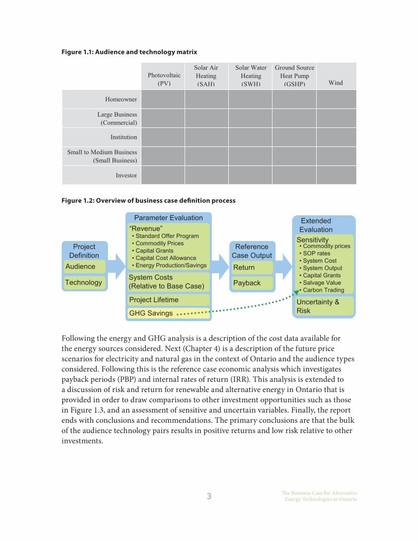
(SWH), ground-source heat pumps (GSHP) and wind power. The audience types considered are homeowner, commercial, small to medium business (small business from here on), institutional and investor. The goal of the investigation is to define the context for investment in alternative energy projects in Ontario in order to encourage interested parties to start their own projects or at least undertake their own feasibility studies. Table 1.1 summarizes the high-level assumptions made about the audience types. For the bulk of the study, the commercial and institutional audiences are examined together, as their characteristics do not differ greatly with respect to the details examined. Figure 1.1 shows the 25 audience and technology pairs that are examined.
Table 1.1: Audience assumptions
Audience type Notes
Homeowner •. Ownership.of.domicile/right.to.perform.interior.and.exterior.modifications
•. Building.type:.detached.and.semi-detached.houses
(Large).Commercial..and.institutional
•. Ownership.of.building(s)/right.to.perform.major.interior.and..exterior.modifications
•. Large.building
Small.business •. Ownership.of.building/right.to.perform.major.interior.and..exterior.modifications
•. Medium-size.building
Investor •. The.investor.is.an.individual.or.body.(such.as.municipalities,.governments.or.investment.firms).
•. Investing.in.renewable.energy.installations.(rather.than.the.manufacture.of.renewable.energy.technologies.themselves)
The report progresses through the steps required to assess the business case for a given installation or audience technology pair. This process is presented graphically in Figure 1.2. This process, and hence this report, begins by defining feasible ranges of energy production and savings for each audience technology pair. As the bulk of the energy and GHG analyses of each of the scenarios are completed with the help of RETScreen (Natural Resources Canada, 2006a), several values provided by RETScreen are used in the analysis. The weather and environmental parameters used for each scenario (as shown in Appendix A) are from RETScreen Toronto data, except for the wind scenarios, where more suitable locations are used (as described in the energy scenarios chapter). In this definition a summary of GHG emission reductions is also included. The GHG values are not included in the reference case calculation, but later in the extended analysis.
3 The Business Case for Alternative Energy Technologies in Ontario
Following the energy and GHG analysis is a description of the cost data available for the energy sources considered. Next (Chapter 4) is a description of the future price scenarios for electricity and natural gas in the context of Ontario and the audience types considered. Following this is the reference case economic analysis which investigates payback periods (PBP) and internal rates of return (IRR). This analysis is extended to a discussion of risk and return for renewable and alternative energy in Ontario that is provided in order to draw comparisons to other investment opportunities such as those in Figure 1.3, and an assessment of sensitive and uncertain variables. Finally, the report ends with conclusions and recommendations. The primary conclusions are that the bulk of the audience technology pairs results in positive returns and low risk relative to other investments.
Figure 1.2: Overview of business case definition process
Figure 1.1: Audience and technology matrix

4The Business Case for Alternative Energy Technologies in Ontario
Figure 1.3: Risk versus return of various investments Adapted.from.Romm.(1999)

5 The Business Case for Alternative Energy Technologies in Ontario
ChAPTER
2Energy Scenarios: Defining Typical Technology Installations
2.1 Introduction
This chapter provides the assumptions and parameters that specify typical building characteristics for each audience type, and the energy systems. The parameters used are in large part values that represent the best case scenario, e.g., buildings are oriented to maximize solar radiation. In other instances, typical average parameters are used, e.g., the reference residential building size is based on a national average. The chapter concludes with a summary of the energy systems for each audience type.
2.2 Building definitions
The five audience types and their associated buildings are described here. These descriptions determine the required or possible sizing of the alternative energy systems. Where possible, building characteristics from Etcheverry (2004) are used in this study, as they are generally based on national or provincial averages. For the purposes of analysis, the buildings are located in the Greater Toronto Area (GTA), at latitude 43.7º and longitude -79.4º. The exception to this is the analysis of the wind energy scenarios, as a more suitable location is required. This detail is discussed further in the Wind section (2.3.4) of this chapter.
2.2.1 homeowner
For the homeowner, a single-family home is used with floor space of 185 metres squared (m²) over two full stories and a basement. The heat load of the building is 8.8 kilowatts (kW) and the cooling load is 9.9 kW. The size and orientation of the roof allow for a 20 m2 photovoltaic array and a 6 m2 solar water collector—both south-facing. Finally, the ventilation demand of the residence is 144 cubic metres per hour (m3/h) and the hot water demand is 240 litres per day (L/day), based on four individuals. All sizing values listed here are from Etcheverry (2004), except for the water and air demands, which come from RETScreen.

�The Business Case for Alternative Energy Technologies in Ontario
2.2.2 Commercial and institutional
The commercial and institutional building has 9,290 m² of floor space over five full stories. The heat load of the building is 212.5 kW and the cooling load is 599.5 kW. The size and orientation of the roof allow for a 728 m2 photovoltaic array and a 45 m2 solar water collector—both south-facing. Finally, the hot water demand of the building is 2,685 L/day and the ventilation demand is 9,222 m3/h. All sizing values listed here are again from Etcheverry (2004), except for the water and air demands, which are from RETScreen.
2.2.3 Small business
The commercial and institutional building has 1,460 m² of floor space over three full stories. This size is based on an average size for Ontario from Natural Resources Canada (NRCan) (2004). The heat load of the building is 39.3 kW and the cooling load is 95.2 kW. The size and orientation of the roof allow for a 144 m2 photovoltaic array and a 7 m2 solar water collector—both south-facing. Finally, the hot water demand of the buildings is 422 L/day and the ventilation demand is 1,449 m3/h. The building parameters are a result of scaling down the commercial/institutional building parameters.
2.2.4 Investor
The investor model does not include a specific building type. This audience type is structured to look at the investment opportunities in using space on buildings from the other audience types.
2.3 Energy systems
The five types of energy systems are described below. The key design variables are specified and the expected annual energy output and GHG emission savings are determined. Each system includes a specific energy value that describes how much energy it delivers and saves per unit, when the unit is a characteristic variable for the given type of system (e.g., per square metre of panel). This specific energy value is used in the business case analysis to scale the price and size of the unit for each of the audience types.
2.3.1 Photovoltaics
The photovoltaic system considered is grid-connected with fixed array, south-facing orientation and panel slope of 32.7º. This orientation and slope maximize annual energy output of the system based on the latitude and longitude of the project. The cells considered are Mono-Si with efficiencies of ŋ=16.1%. These parameters are the same

� The Business Case for Alternative Energy Technologies in Ontario
as those used in the Toronto photovoltaic cooperative feasibility study performed by Toronto Renewable Energy Co-operative (TREC) (2007).
The remaining parameter values are inverter efficiency and miscellaneous losses. Inverter efficiency is assumed to be 94 per cent and miscellaneous losses 11 per cent. Photovoltaic degradation is not explicitly included in the model as RETScreen does not provide this functionality. However, this limitation is partly mitigated by using a slightly higher value for miscellaneous losses. A more explicit degradation model would include more degradation at the beginning of the project life and less at the end.
Based on the above parameters, as the system scales in size, its electricity and power capacity scale linearly by factors of 0.192 and 0.161 respectively as shown in Figure 2.1.
Figure 2.1: PV system scaling with respect to collector areaThe.annual.output.(MWh).and.capacity.(kW).of.the.PV.systems.can.be.calculated.from.the.collector.area.using.the.values.found.in.this.regression.
Calculating the GHG emission reductions associated with using a PV system in Ontario can be accomplished using several methods. For the purposes of this study, proposed guidelines from the Alberta Government (2008), the United Nations Framework Convention on Climate Change (UNFCC) (2006) and the UNFCC (2008) are used. The use of these sources is relevant as the policies developed under the proposed Canadian GHG offset trading system are likely to incorporate them (Environment Canada, 2008a).
The guidelines suggest various methods for calculating GHG reductions from the use of renewable energy. For this study the average GHG emission rate from the Ontario electricity grid is used, this value being 0.23 kilograms of carbon dioxide equivalent per kilowatt hour (kgCO2-eq/kWh) based on data from Ontario Power Authority (OPA) (2007) and including nine per cent losses from transmission and distribution. Although
�The Business Case for Alternative Energy Technologies in Ontario
other methods suggested by the guidelines are more desirable, this method is the simplest and provides a fair approximation. Ideally a marginal value would be used based on historical data from the electricity grid. In this context, marginal refers to peak energy production, since it is the generally higher emitting and more expensive sources that are likely supplanted by the alternative energy source. Thus, the average value used here is likely a lower estimate of the GHGs offset or eligible-for-offset accounting.
2.3.2 Solar air heating
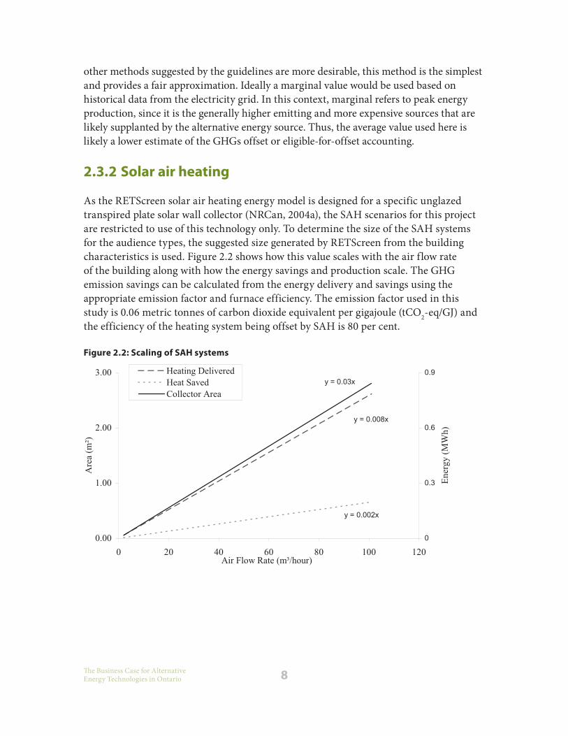
As the RETScreen solar air heating energy model is designed for a specific unglazed transpired plate solar wall collector (NRCan, 2004a), the SAH scenarios for this project are restricted to use of this technology only. To determine the size of the SAH systems for the audience types, the suggested size generated by RETScreen from the building characteristics is used. Figure 2.2 shows how this value scales with the air flow rate of the building along with how the energy savings and production scale. The GHG emission savings can be calculated from the energy delivery and savings using the appropriate emission factor and furnace efficiency. The emission factor used in this study is 0.06 metric tonnes of carbon dioxide equivalent per gigajoule (tCO2-eq/GJ) and the efficiency of the heating system being offset by SAH is 80 per cent.
Figure 2.2: Scaling of SAh systems

� The Business Case for Alternative Energy Technologies in Ontario
2.3.3 Solar water heating
The three system sizes of interest are shown in Table 2.1. The SWH scenario uses a pump power rating of 50W per metre squared (/m2) of solar collector area and assumes an efficiency of 75 per cent from a natural gas conventional system. The energy savings in Table 2.1 are from Hargreaves (2008) and are similar to values from Kapoor (2008).
Table 2.1: SWh system characteristics
homeowner Commercial/institutional Small business
Demand.(L/day) 240 2,685 422
Collector.area.(m2) 6 46 8
Energy.savings.(MWh/a) 2.9 32.6 5.7
2.3.4 Wind
The wind scenarios consist of a single turbine for each audience type. The details of each system appear below in Table 2.2. The turbine sizes selected are roughly representative of the sizes that each audience type could be expected to afford.
Table 2.2 Summary of energy scenarios for wind
Power (kW) hub height (m)
Homeowner 2.6 20
Commercial/institutional 50 25
Small.business 10 24
As mentioned previously, the location of the wind turbine scenarios differs from the other technology scenarios. A more rural area with a high wind speed is more suitable for the installation of a wind turbine. Thus, this study does not use the GTA to locate the wind scenario. Instead, a best case location is chosen based on the average wind speeds in Ontario. Using data from the Canadian Wind Energy Atlas, a distribution of wind speeds in Ontario was constructed (Figure 2.3). This study uses a wind speed of 5.9 metres per second (m/s), that corresponds roughly to the highest peak in this distribution.

10The Business Case for Alternative Energy Technologies in Ontario
Using the above data the annual energy output and GHG emission reductions are calculated and tabulated in Table 2.3. The emission factor of 0.23 kgCO2-eq/kWh from the PV case also applies to this case. Wind is also assumed to offset centralized grid electricity production.
Table 2.3: Wind energy output and GhG emission savings
Annual output (MWh) Annual GhG reductions (tCO2-eq)
Homeowner 4.9 1.1
Commercial/institutional 129.4 29.8
Small.business 12.2 2.8
2.3.5 Ground-source heat pumps
The differences from conventional systems are important details for describing the business case for GSHP systems. The first difference, discussed here, is the annual energy savings and GHG emission reductions that these systems produce. The second important difference, system cost, is discussed in Chapter 3.
The cooling and heating power ratings of the buildings discussed in the first section of this chapter are used to size the conventional and GSHP systems, and to determine the space conditioning profiles of the buildings. Another important consideration for
Figure 2.3: Ontario wind speed distributionThe.distribution.is.calculated.from.a.set.of.over.45,000.data.points.provided.by.the.Canadian.Wind.Energy.Atlas.Model.(Environment.Canada,.2003)..The.data.set.was.filtered.using.GIS.software.to.extract.only.those.points.of.data.over.land,.as.offshore.wind.turbines.are.not.considered.in.this.study.

11 The Business Case for Alternative Energy Technologies in Ontario
sizing GSHP systems is deciding what trade-off to make between the capital costs of the system and the desired annual energy savings. This trade-off exists because less capital is required if the GSHP system is supplemented with a backup conventional system that operates during stages of peak demand. For this study, the homeowner’s system is approximately sized to 70 per cent of peak demand (including hot water) while the other cases are sized to approximately 75 per cent of peak cooling demand as recommended by NRCan (2000) and NRCan (2002) respectively. The details of the systems, with reference to the base case or common system, are summarized in Table 2.4.
Table 2.4: GShP scenario definition
homeowner Commercial/institutional Small business
Base case
.....Heating.system.fuel.type Natural.gas Natural.gas Natural.gas
.....Heating.system.efficiency.(%) 80 80 80
.....Cooling.system.fuel.type Electricity. Electricity Electricity
.....Cooling.system.COP 4 4 4
.....Annual.electricity.usage.(MWh) 3.7 223.4 35.5
.....Annual.natural.gas.usage.(m3) 2,628 55,180 10,205
Proposed case
.....GSHP.heating.efficiency.(%) 330 300 300
.....GSHP.cooling.COP 4.2 3.9 3.5
.....Peak.cooling.system.fuel.type -- Electricity Electricity
.....Peak.heating.system.fuel.type Electricity -- --
.....Peak.cooling.COP -- 4.0 4.0
.....Peak.heating.efficiency.(%) 80 -- --
.....Annual.electricity.use.(MWh) 10.3 382.2 68.5
2.4 Summary
The building descriptions and energy system characteristics defined throughout this chapter result in the energy scenarios summarized in Table 2.5. The values in this table are combined with the system cost data defined in the next chapter, and natural gas and electricity price projections are described after that in order to define the business case for these technology audience pairs.

12The Business Case for Alternative Energy Technologies in Ontario
Table 2.5: Summary of energy scenarios
System characteristic PV SAh SWh Wind GShPh
omeo
wne
r
Collector.area.(m2) 20 4 6 -- --
Power.capacity.(kW) 3.2 -- -- 2.6Heat=8.8.Cool=9.9
Annual.energy.output/savings.(MWh) 4.2 1.8 2.9 4.9 21.0
Annual.GHG.emission.savings.(tCO2-eq) 1.0 0.3 1.1 1.1 4.9
Com
mer
cial
/ins
titu
tion
al Collector.area.(m2) 728.. 256 46 -- --
Power.capacity.(kW) 117 -- -- 50Heat=213.Cool=600
Annual.energy.output/savings.(MWh) 150.7 112.2 32.6 129.4 420.5
Annual.GHG.emission.savings.(tCO2-eq) 34.7 20.1 12.5 29.8 103
Smal
l bus
ines
s
Collector.area.(m2) 117 40 8 -- --
Power.capacity.(kW) 18.4 -- -- 10Heat=39.Cool=95
Annual.energy.output/savings.(MWh) 22.5 14.6 5.7 12.2 74.1
Annual.GHG.emission.savings.(tCO2-eq) 5.2 3.1 2.2 2.8 19

13 The Business Case for Alternative Energy Technologies in Ontario
ChAPTER
3 Financial Data
3.1 Introduction
Part of building any business case includes defining cost estimates and their variations. For fairly new and diverse investments, as considered here, this necessitates using data from several sources. This chapter presents the available system costs for photovoltaic, solar air heating, solar water heating, ground-source heat pump and wind systems. The pertinent cost categories for this study are total installed cost, annual operation and maintenance (O&M) costs where applicable, and sources of financial assistance. Total installed costs include the price of equipment, labour and any other necessary initial services. If O&M costs are not discussed, it is assumed that they are negligible or negligible compared to the base case. Sources of financial assistance include capital grants available from the government, feed-in tariff rates available through the Ontario Standard Offer Program and capital cost allowance regulations.
3.2 Cost data3.2.1 Photovoltaics
Although it is known that prices of photovoltaic modules have been steadily dropping by about five per cent per year (CanSIA, 2005), there is difficulty in assessing the final total installed cost for grid-connected PV systems including labour, balance of system and administrative costs. Data from 2006 show that the total installed prices are decreasing (Table 3.1) and, more recently, in a study for Environment Canada (Bailie, et al., 2007), an installed price of $9.50 per watt (/W) was used to model the economics of PV in Canada. This latter number roughly agrees with the decreasing trend in cost shown in Table 3.1.
Table 3.1: Installed prices of solar PV in Canada Adapted.from.Ayoub.(2006)
$/watt 1��� 2000 2001 2002 2003 2004 2005 200�
Grid-connected..(≤.10.kW).
21. 20. Insufficient.data
Insufficient.data
Insufficient.data
14.5. 10. 10
Grid-connected.(>10.kW).
No.data
No.data
Nodata
Nodata
Nodata
No.data.
12.6 10

14The Business Case for Alternative Energy Technologies in Ontario
More recent data on the total installed cost of PV systems for residential installations in bulk purchase programs are shown in Table 3.2. These data come from a community initiative in the City of Toronto that arranged bulk purchases and installation of PV systems for a group of homeowners. It shows that for systems greater than 1kW, prices around the $9.50/W mark are achievable on these smaller scales for homeowners who purchase as a group. It is assumed that the installed price for individual homeowners is closer to $11/W.
Table 3.2: Installed residential PV costs Adapted.from.Traynor.(2008)
Capacity (kW) Cost/watt ($)
1 $12.5–$15.5
2 $9.5–$10.5
3 $9–$10.2
In summary, the price of $9.50/W installed is the most recent price available, it agrees with historic decreasing trends, and it is used for this study as the PV reference price. However, this price is not reasonable for small individual residential installations. For the homeowner case, a price of $11/W is more realistic.
3.2.2 Solar air heating
Natural Resources Canada’s Renewable Energy Deployment Initiative (REDI) program ended in 2007. It provided financial support for 25 per cent of the (eligible) capital cost of renewable energy systems up to a maximum of $80,000 for non-residential installations (Kapoor, 2008). The average system costs (the gross of REDI funding) and cost standard deviation by year from the program are shown in Figure 3.1. (Further data from REDI are available in Appendix B.) This study uses the data for the last year of the program for the SAH reference cost and the cost standard deviation, of $373/m2 and $203/m2 respectively. This choice was made as the final year of the program includes the largest sample population (number of systems installed) and since the data do not indicate a strong trend over the course of the program. Also, notice that this price is used for all audience types and that no data exist that illustrate there are economies of scale in the system cost.

15 The Business Case for Alternative Energy Technologies in Ontario
3.2.3 Solar water heating
Cost data for SWH systems also come from the REDI program. The SWH installed system costs from the REDI program are shown in Table 3.3. Of note is the average cost of $1,032.73 and $1,374.80/m2 for glazed and evacuated tube systems respectively. The glazed prices are used in this study for all the audiences.
Table 3.3: Sample SWh REDI installation characteristics from 1���–200� (Kapoor, 200�)
Technology No. of systems
Average collector area (m2)
Average cost/m2 ($)
Cost fit (R2) Cost standard deviation ($/m2)
Glazed 78 44.6 1,033. 0.84 425
Unglazed 27 143.7 198 0.77 53.9
ETC 10 37.8 2165. Unavailable 1,118
3.2.4 Wind
As described in Chapter 2, the wind installations considered in this study are for single turbine installations ranging in size from 2.6 kW to 50 kW. Cost data specific to each class of turbine are required as costs are scale dependent. For these costs, a survey of the Canadian market in 2005 is used, as summarized in Table 3.4. For the 10 kW and 50 kW systems studied in this report, the installed cost and annual operation and maintenance (O&M) costs are taken directly from this table. For the 2.6 kW case, the costs are interpolated between the 1 kW and 10 kW systems. The 1 kW system is meant for battery charging and, thus, the interpolation may lead to slightly high estimates. The resulting costs for the 2.6 kW system are $17,580 and $335 per year for the capital and O&M costs respectively.
Figure 3.1: SAh cost trends from REDI

1�The Business Case for Alternative Energy Technologies in Ontario
Table 3.4: Small turbine costs in 200� dollarsAdapted.from.Marabek.(2005)..Inflation.adjusted.to.2008.dollars.
1.kW 10.kW 50.kW
Application Battery.charging Battery.charging.or.on-grid On-grid
Turbine.cost $3,012 $34,964 $118,340
Installation.and.BOS.cost $3,873 $27,003 $59,170
Total.installed.cost $6,885 $61,967 $177,510
Total.cost.per.kW $6,885 $6,197 $3,550
Annual.O&M.cost $140 $1,237 $3,550
3.2.5 Ground-source heat pumps
For the GSHP case, the cost data collected represent the differential over installing a conventional heating system. Several sources for this information have been consulted for this study. The following first examines sources that discuss differential operation and maintenance (O&M) costs compared to traditional space conditioning systems. The second discusses sources that look at the differential installed cost.
Differential operation and maintenance costs
A comprehensive survey of GSHP operation and maintenance costs for non-residential installations is available in Cane and Garnet (2000). The paper provides a summary comparison of the annual O&M costs of GSHP and other space conditioning systems. The data are presented graphically in Figure 3.2 and shows the large annual savings (a factor of 10 to 20) that GSHP provides compared to conventional systems.
Figure 3.2 illustrates the absolute O&M costs, whereas for the economic analysis the differential is required. This differential is calculated by taking the average of the non-GSHP space conditioning systems and subtracting the average of the different GSHP maintenance methods. This result gives a differential annual savings of $4.43/m2 of floor space per year. This number is viewed as the average case and serves as the estimate for this study. When performing an economic assessment for a specific building installation, a more rigorous estimation will likely be required, especially in the case of an existing building. Note that this estimate may be low since the use of a GSHP system removes the need for both a heating and cooling system, and only a comparison to the cooling systems is used in the calculation.
The estimate developed above is for non-residential audience types. It is assumed that the difference in O&M costs for residential circumstances is negligible.

1� The Business Case for Alternative Energy Technologies in Ontario
Differential total installed costs
RETScreen and the Ontario government provide data comparing the installed cost of various space conditioning systems for commercial and residential systems respectively. These data, combined with market experience, show the cost differential is around 3:1 for homeowners and 2.4:1 for other audiences (Schafer, 2008). Hence, the GSHP costs are as shown in Table 3.5, for the building sizes considered.
Table 3.5: Differential GShP costs†.Total.installed.costs,.adapted.from.RETScreen.and.assuming.2.4:1.incremental.cost.*.Heat.pump.costs,.adapted.from.Government.of.Ontario.(2007).and.assuming.a.3:1.incremental.cost.
Audience Differential install cost ($/m2 of floor space)
Notes
Homeowner 61.6* Relative.to.80.per.cent.natural.gas.furnace
Commercial/institutional 39.7† Relative.to.average.cost.of.conventional.systemsSmall.business 40.4†
The costs for GSHP in non-residential buildings can be further broken down by equipment components as shown in Table 3.6.
Figure 3.2: Space conditioning annual O&M costs by type for commercial buildings Adapted.from.Cane.(2000)

1�The Business Case for Alternative Energy Technologies in Ontario
Table 3.�: Non-homeowner GShP equipment costsAdapted.from.RETScreen
Average unit cost ($/unit) Unit
Circulating.pump . 550 kW.of.Pump.Power.
Circulating.fluid . 2950 m³.of.fluid
Drilling.and.grouting . 56 m.of.drilling
Loop.pipe . 3 m.of.pipe
Fittings.and.valves . 9 kW.of.cooling.capacity
GSHP . 450 kW.of.power
3.3 Sources of financial assistance3.3.1 Government funding
There are two sources of government grants available for SAH and SWH systems for non-homeowner installations. The first is the federal government program that replaced REDI—ecoEnergy. The renewable heat arm of this program, as of April 2007, provided a grant of 25 per cent for the capital cost of SAH and SWH systems up to a maximum of $80,000 (Government of Canada, 2008a). The rules of this program have been updated for September 2008. However, these new rules, which include changes to the subsidies, have not been included in this study. Projects in Ontario that qualify for this program are also eligible for a grant from the provincial government under the Ontario Solar Thermal Heating Incentive (OSTHI). This program offers additional support of 25 per cent for the capital cost of SAH and SWH systems up to a maximum of $80,000 (Government of Canada, 2008b). These grant amounts are included in the analysis of non-homeowner SAH and SWH scenarios.
There are also grants available under ecoEnergy programs for wind and PV installations, but the minimum size of eligible installation is well beyond those considered in this study.
3.3.2 Standard Offer Program
Under the Standard Offer Program (SOP) in Ontario, PV and wind projects can be guaranteed a feed-in tariff rate of $0.42 per kilowatt hour (/kWh) and $0.11/kWh respectively for 20 years. These rates, however, are the initial tariff rates of the program. At the time of this writing the program is undergoing a restructuring that may impact the rates. These rates are the source of income for PV and wind projects in this study. Other techniques can be used, such as net metering of energy demand. However, as there is much uncertainty in the future price of electricity, the scenarios in this report were constructed using the SOP rates in order to mitigate this uncertainty.

1� The Business Case for Alternative Energy Technologies in Ontario
3.3.3 Capital cost allowance
Under tax regulations, the non-homeowner projects are eligible for capital cost allowance. The capital cost allowance is included in this study by the use of the capital cost tax factor (CCTF), a mechanism that allows for the future benefit of tax savings from depreciation to be incorporated into an economic analysis. Capital cost tax factor can be calculated in the following two ways (Fraser et al., 2000):
(3.1)
(3.2)
In this formula, t is the income tax rate (16.5 per cent for small business and 33.5 per cent for commercial/institutional), d the CCA rate (30 per cent for wind and PV and four per cent for other technologies) and i the after-tax interest rate. For the after-tax interest rate, a before-tax value of 10 per cent is used and adjusted by a factor of (1-t).
In equation (3.1), CCTFnew is used to calculate the tax benefits for all time and accounts for the half-year rule. Capital cost tax factor old, in equation (3.2) is necessary when the projects do not last for all time. Capital cost tax factor old is used to account for this by adjusting for the salvage value. In this study the reference case, however, assumes a salvage value of zero.
( )( )( )new
ttd 1 dCCTF 1i d 1 i
+= −
+ +
oldtd CCTF 1
i d= −
+

20The Business Case for Alternative Energy Technologies in Ontario
3.4 Summary
In this chapter, the costs of alternative energy systems under examination in this study were presented along with sources of financial assistance. The cost data used in the economic analysis to follow are summarized in Table 3.7 and Table 3.8.
Table 3.�: Summary of cost data
Reference (mean) installed cost ($/unit) Standard Deviation (% of cost)
Standard Deviation ($/unit)homeowner Commercial/
institutionalSmall
business
PV . 11.0/W . 9.5/W . 9.5/W . 47.9 . 4.6/m2
SAH . 372.7/m2 . 372.7/m2 . 372.7/m2 . 54.6 . 203.4/m2
SWH . 1,032.7/m2 . 1,032.7/m2 . 1,032.7/m2 . 41.2 . 425.0/m2
Wind . 6.8/W . 3.6/W . 6.2/W . 47.9 . Varies
GSHP . 50.3/m2 . 46.6/m2 . 48.4/m2 . 47.9 . Varies
Table 3.� Incremental annual O&M costs ($)
homeowner Commercial/institutional Small business
PV . Negligible . Negligible . Negligible
SAH . Negligible . Negligible . Negligible
SWH . Negligible . Negligible . Negligible
Wind . 335 . 3,550 . 1,237
GSHP . Negligible . -41,149 . -6,467

21 The Business Case for Alternative Energy Technologies in Ontario
ChAPTER
4 Energy Price Forecasts
4.1 Introduction
As many of the energy systems considered in this study replace or divert demand for natural gas and centralized grid electricity, changes in the price of these traditional sources will affect the business case for the new sources. To address this issue, this chapter presents a summary of various future natural gas and electricity price scenarios and the structure of customer billing of these commodities in Ontario. The chapter also discusses the methodology used to select a meaningful price projection for this study, as well as a range of possible prices that affect the risk of investment in alternative energies. Note that, unless otherwise stated, all prices are in 2008 dollars.
4.2 Billing structure
The first step to understanding the effect of natural gas and electricity price on alternative energy investments is to understand how users of these commodities are impacted by price changes. The following section describes the billing structure of these commodities in Ontario and offers a perspective on how these conditions may change during the project time frame considered here.
The prices that natural gas and electricity customers in Ontario pay are comprised of several charges, most of which are controlled by a provincial governmental body called the Ontario Energy Board (OEB). This board dictates the prices that distribution companies are allowed to charge end-customers in various parts of the province. This study focuses on these charges in the GTA context.
End users are broken up into several categories or billing groups depending on their energy demand and their market segment (e.g., homeowner). For the energy scenarios in this study the audience types can be grouped into two natural gas and three electricity price brackets, as shown in Table 4.1. Each of these customer types has a different billing structure and is charged different rates accordingly.

22The Business Case for Alternative Energy Technologies in Ontario
Table 4.1: Energy customer type breakdownThe.power.ratings.for.the.electricity.types.refer.to.monthly.average.peak.demand.
homeowner Commercial/institutional Small business
Natural.gas Residential General.service General.service
Electricity Residential General.service.50.to.999kW General.service.<.50.kW
This distinction of customer type is important as it breaks down the commodity charges from the other service charges. This allows for a proper evaluation of the savings realized through the reduction in demand of the commodity. This distinction is clearer when the customer fees are defined, as in Table 4.2 for natural gas. There are two important things to note in this table. The first point is that the customers are billed differently and that they are charged twice for their energy demands—once for the commodity and once for the delivery of the commodity. The second point is that since the economic analysis deals with a difference in demand, the monthly charges can be ignored as they cancel out in the subtraction, unless the use of a new alternative energy source entirely removes the demand for a commodity.
Table 4.2: Natural gas billing structure comparison for April 200�Adapted.from.OEB.(2008)
Residential General service
Monthly.customer.charge.($) 14 Monthly.customer.charge.($) 50
Gas.charge.($/m³) 0.390 Gas.charge.($/m³) 0.391
Delivery.charge.per.m³: Delivery.charge.per.m³:
.For.the.first.30.m³.($/m³) 0.152 .For.the.first.500.m³.($/m³) 0.133
.For.the.next.55.m³.($/m³) 0.146 .For.the.next.1,050.m³.($/m³) 0.116
.For.the.next.85.m³.($/m³) 0.142 .For.the.next.4,500.m³.($/m³) 0.103
.For.all.over.170.m³.($/m³) 0.138 .For.the.next.7,000.m³.($/m³) 0.095
.For.the.next.15,250.m³.($/m³) 0.092
.For.all.over.28,300.m³.($/m³) 0.091
4.3 Forecasts
Two pieces of information are needed to project what end-customers will be paying for the use of these commodities over the project life. The first is the price of the non-commodity fees, such as delivery charges, and the second is the price of the commodities themselves.

23 The Business Case for Alternative Energy Technologies in Ontario
4.3.1 Non-commodity fees forecasts
The non-commodity fees for natural gas are assumed to remain constant for all customer types. This assumption is based on historical patterns, of which the residential pattern is shown as an example in Figure 4.1.
Figure 4.1: historical residential natural gas fees vs. commodity priceThe.non-commodity.fees.remain.nearly.constant.with.respect.to.time..The.equation.illustrates.the.linear.fit.for.the.first.30m3.delivery.fees..The.slope.of.the.line.is.nearly.zero..Adapted.from.OEB.(2008).
For the non-commodity fees associated with the use of electricity, a combination of OPA forecasts and linear interpolations is used to forecast the non-commodity fees. The linear interpolations are required as the OPA projections are in five-year increments. The residential electricity fee projections are shown in Figure 4.2.
4.3.2 Commodity price forecasts
Natural gas
Two steps are required to forecast OEB natural gas prices. The first is the collection of natural gas price forecasts from the available literature, as modeling such forecasts is outside the scope of this study. The second step is to convert these forecasts into OEB prices. This second step is required as natural gas prices in North America can be referenced at several different places. The reference point used in this study is the Alberta provincial natural gas price. The transformation from the Alberta price to OEB prices is a shifted linear transformation, as illustrated in Figure 4.3.

24The Business Case for Alternative Energy Technologies in Ontario
The price forecasts for step one appear in Figure 4.4. The data in this figure have been converted to the Alberta reference. The original forecasts were for prices referenced at the Henry Hub and the United States Wellhead. To transform natural gas prices from Henry Hub prices to Wellhead prices, the Henry Hub prices are reduced by the mean difference between historical Henry Hub and Wellhead prices (Budzik, 2003), a process used by the OPA in their long-term Integrated Power Systems Plan (IPSP). This process is also used to convert the Wellhead prices into the Alberta reference.
Figure 4.2: Residential electricity fee projections Adapted.from.OPA.(2007)
Figure 4.3: Alberta/OEB natural gas price transformation

25 The Business Case for Alternative Energy Technologies in Ontario
The price used in the reference case of this study is $0.388 per metre cubed (/m3) (transformed to the OEB price) or $0.286/m3 based on Alberta prices (Sproule, 2008). This value comes from the average Alberta price from 1995 to the present. As can be seen in Figure 4.4, this price roughly represents the average price of the forecasts. It also represents the approximate average OEB price since 2003 after being transformed (Figure 4.3).
Figure 4.4: Natural gas price forecasts (adjusted to Alberta price)Adapted.from,.NEB.(2007),.Greenpeace.and.EREC,.2007.(2007),.EIA.(2007),.OPA.(2007),.NRCan.(2007),.IEA.(2004),.NPC.(2007),.Enbridge.(2007).
Electricity
For forecasting the commodity price of electricity in Ontario for the project period, the forecast from the OPA IPSP (OPA, 2007) is used. Again, interpolation between the five-year points is required to complete the annual forecast (Figure 4.5). The OPA forecast includes a measure of variation in its maximum and minimum projections, as indicated with the error bars in the figure.

2�The Business Case for Alternative Energy Technologies in Ontario
To use the commodity price in the analysis, this price must be converted into the form used by the OEB to set end-customer prices. The OEB sets two commodity prices: a price charged for an initial allotment of electricity use per month and another price for the amount used above this allotment. For this study it is assumed that this pricing scheme will continue for ease of calculation. In actuality, all customers will likely be changed to a peak power pricing model, however, this model was found not to substantially affect the outcome of this study, and is thus not used due to its computational intensity.
To convert the commodity price to these two values, the following formulae are used:
(4.1)
(4.2)
Where,
Phigh.is.the.price.paid.over.the.monthly.threshold;.
Plow.is.the.price.paid.below.the.threshold;
Pcommodity.is.the.commodity.cost.of.electricity;.
∆high-low.is.the.difference.between.the.two.prices.(OEB.maintains.this.value.at.9$/MWh);
n.and.d.are.the.number.of.customers.and.their.total.demand.respectively.(residential.values.projected.by.OEB.are.used);.and
T.is.the.threshold.(a.static.value.of.750kWh.is.used,.although.OEB.changes.the.value.throughout.the.year.for.different.customers).
Figure 4.5: Electricity commodity price forecast (OPA, 200�)
high commodity high lowP P T n d−= + ∆ ⋅ ⋅
low high high lowP P −= − ∆

2� The Business Case for Alternative Energy Technologies in Ontario
4.4 Commodity price uncertainty
Although sensitivity to commodity price changes can easily be tested by using the expected range of values, testing the uncertainty with a probabilistic method is better equipped to quantify the possible outcomes.
This is performed by examining the stochastic nature of the historical commodity prices, and assuming that both the natural gas and electricity prices are random walks. Thus, the first difference can be taken and tested statistically to determine which, if any, probability distribution the year-to-year price change exhibits. In doing this test it was determined that this distribution for both is a Laplace distribution. With this distribution specified, random projections can be generated for the project lifetime. These random projections are generated several times in the Monte Carlo analysis described in the following chapter that quantifies the overall uncertainty of investing in each of the scenarios impacted by these commodities.
4.5 Summary
This chapter presented the billing structure for users of electricity and natural gas, projections of what will happen to these bills and the commodity prices, and how these values can be tested in the economic, sensitivity and uncertainty analyses. The results appear in the following chapter.

2�The Business Case for Alternative Energy Technologies in Ontario
ChAPTER
5 Business Case
5.1 Introduction
This chapter presents the results of the economic analysis. The analysis begins with a reference case that provides the internal rates of return (IRR) and pay-back periods (PBP) of each of the audience technology pairs under the reference data and assumptions laid out in the previous chapters. This is followed by the sensitivity analyses and uncertainty analyses. Note that the project life is 20 years for all technologies; although some may have a slightly longer usable lifetime, it was assumed that the use of a shorter lifetime has a negligible impact due to the time value of money. This assumption is tested later in this chapter.
The results indicate that a wide range of IRRs and PBPs exists among the audience technology pairs. This is to say that some are quantitatively very good investments, while others are not. There are many other aspects that are not considered in the analysis such as the marketing value of investing in green technologies or the desire to invest in green technologies simply in a desire to reduce one’s environmental footprint. In this later case, all that may be important is that the returns are slightly positive. The methodology, data used and results presented in the remainder of the chapter serve as a baseline for understanding economic returns.
5.2 Reference case
The reference case results (Table 5.1) consist of the IRRs and PBPs for the set of audience technology pairs, excluding the investor cases, as these are defined after the uncertainty analysis. The cells of the table with no values are for those projects with a negative IRR.
2� The Business Case for Alternative Energy Technologies in Ontario
Table 5.1: Reference case internal rates of return (%) and pay-back periods (years)
homeowner Commercial Institutional Small business
PV -- 1.5%,.16.9 1.5%,.16.9 --
SAH 1.7%,.16.8 10.9%,.8.0 10.9%,.8.0 10.1%,.8.4
SWH -- 5.9%,.11.5 5.9%,.11.5 5.8%,.11.7
Wind -- 3.6%,.13.3 3.6%,.13.3 --
GSHP 6.4%,.11.0 12.4%,.7.2 12.4%,.7.2 14.7%,.6.3
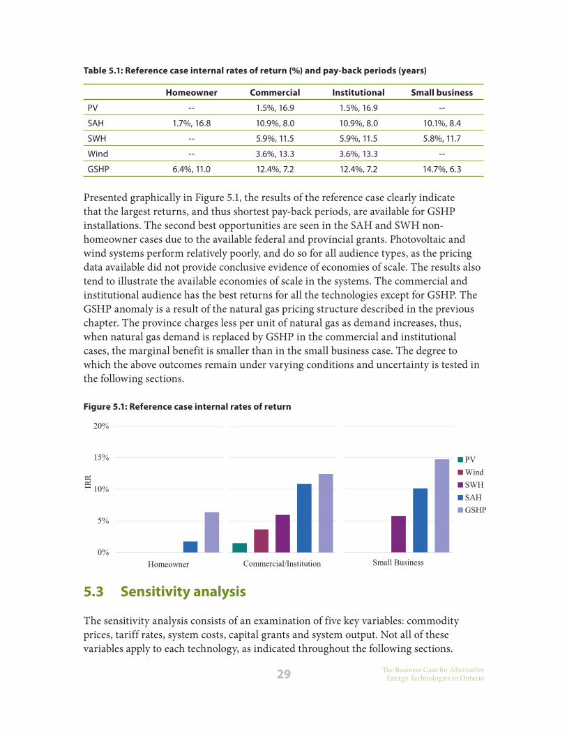
Presented graphically in Figure 5.1, the results of the reference case clearly indicate that the largest returns, and thus shortest pay-back periods, are available for GSHP installations. The second best opportunities are seen in the SAH and SWH non-homeowner cases due to the available federal and provincial grants. Photovoltaic and wind systems perform relatively poorly, and do so for all audience types, as the pricing data available did not provide conclusive evidence of economies of scale. The results also tend to illustrate the available economies of scale in the systems. The commercial and institutional audience has the best returns for all the technologies except for GSHP. The GSHP anomaly is a result of the natural gas pricing structure described in the previous chapter. The province charges less per unit of natural gas as demand increases, thus, when natural gas demand is replaced by GSHP in the commercial and institutional cases, the marginal benefit is smaller than in the small business case. The degree to which the above outcomes remain under varying conditions and uncertainty is tested in the following sections.
Figure 5.1: Reference case internal rates of return
5.3 Sensitivity analysis
The sensitivity analysis consists of an examination of five key variables: commodity prices, tariff rates, system costs, capital grants and system output. Not all of these variables apply to each technology, as indicated throughout the following sections.

30The Business Case for Alternative Energy Technologies in Ontario
The goal of the analysis is to gauge the effect of these variables on the suitability of investment for the audience technology pairs. The data produced by this examination are useful in assessing the viability of an individual project under varying circumstances or different expectations in future commodity prices.
5.3.1 Commodity prices
As described in the previous chapter on commodity prices, the economics of SAH and SWH are impacted in the scenarios constructed here by the price of natural gas, while GSHP projects are impacted by both natural gas prices and electricity prices. The sensitivity of the investments to these commodity prices is tested with results shown below.
Figure 5.2 illustrates the natural gas price sensitivity for the homeowner cases, while Figure 5.3 illustrates this test for commercial, institutional and small business audience members. The curves illustrate the IRR resulting from a specified average annual increase of natural gas prices. Also shown are the IRRs resulting from the natural gas price forecasts described in Figure 4.4. These IRRs are fit to the average annual gas price increase curve in order to draw comparisons.
Figure 5.2: Effects of natural gas price on SAh, SWh and GShP (homeowner)The.solid.lines.indicate.the.average.annual.natural.gas.price.increase.required.to.achieve.a.given.IRR..The..indicate.the.IRR.and.comparable.natural.gas.price.change.realized.from.various.natural.gas.price.projections.(as.documented.in.Chapter.4)..This.graph.illustrates.that.under.the.reference.conditions.it.is.likely.that.SAH,.SWH.and.GSHP.for.these.two.audiences.will.see.at.least.modest.returns.with.respect.to.possible.natural.gas.price.changes.

31 The Business Case for Alternative Energy Technologies in Ontario
The importance of including these fitted points on the curves is that they illustrate how realistic a given IRR may be. For example, in the homeowner SWH case the required annual gas price increase for a positive IRR is so high (~ $0.04/m3) that none of the projections fall on the curve. Or, in other words, the gas price forecasts all produce a negative IRR in the SWH homeowner scenario. Similarly, it can be seen that some of the projections fall on the SAH and GSHP curves. As these price forecasts describe widely varying scenarios that can but may not occur, the best investment choices are those audience technology pairs that produce acceptable IRRs for the most forecasts—as is the case with GSHP for all audience types.
Figure 5.3: Effects of natural gas price on SAh and SWh (commercial/institutional)The.solid.lines.indicate.the.average.annual.natural.gas.price.increase.required.to.achieve.a.given.IRR..The..indicate.the.IRR.and.comparable.natural.gas.price.change.realized.from.various.natural.gas.price.projections.(as.documented.in.Chapter.4)..This.graph.illustrates.that.under.the.reference.conditions.it.is.likely.that.SAH,.SWH.and.GSHP.for.these.two.audiences.will.see.at.least.modest.returns.with.respect.to.possible.natural.gas.price.changes.
(a) Commercial/Institution (b) Small Business
With an understanding of the dependence on natural gas prices for suitability of investment, the next step is to establish such an understanding for electricity prices, with respect to the GSHP case. For this analysis, the commodity price projections made by the OPA (2007) are used. The resulting changes in IRR are presented in Figure 5.4, with differences between high and low cases of about one per cent. As the electricity prices used are from the OPA’s plan to 2027, this outcome can only be realized if this plan is followed.

32The Business Case for Alternative Energy Technologies in Ontario
5.3.2 Sensitivity to tariff rates
The PV and wind tariff rates produce the income for these systems. Since these rates are fixed by the provincial government, testing the sensitivity to them is not entirely relevant to the individual or entity already in the SOP. Results of the sensitivity study are still, however, meaningful since they provide a description of the economic returns if the rates are changed—a likely event at the time of this writing.
Figures 5.5 to 5.7 illustrate the effect a change in the SOP tariff rate would have on the IRR for PV or wind projects. The figure shows that thresholds for positive returns are a tariff rate of about $0.3/kWh for wind and $0.6/kWh for PV (compared to $0.11/kWh and $0.42/kWh for the reference case). Important to note is that a small change in the SOP rate can have a large impact on the IRR of wind projects, while a similar change (in absolute terms) for the PV rate will have less of an effect. This difference is due to the nonlinearity of the time value of money in the IRR calculation.
5.3.3 Capital grantsAs was shown in the reference case, the non-homeowner SWH and SAH cases are made profitable by the available provincial and federal grants. Thus, an assessment of the impact of grants on the 20 reference case scenarios is presented in Figures 5.8 to 5.10 for the different audience types. In these figures, the reference case is illustrated with a black diamond. These graphs are useful for understanding what returns can be expected if grant funding of a given amount becomes available.
A similar pattern to the other sensitivity analyses is shown by this examination. For example, a drastic change in grant amounts is required to achieve an increase in IRR for PV compared to wind. Also, it is shown how the grant is somewhat unnecessary for
Figure 5.4: GShP IRR sensitivity to electricity pricesThe.three.electricity.price.cases.are.those.presented.in.Chapter.5.from.the.OPA.IPSP.(OPA,.2007).

33 The Business Case for Alternative Energy Technologies in Ontario
Figure 5.5: Effect of tariff rates on PV and wind homeowner IRRs
Figure 5.�: Effect of tariff rates on PV and wind small business IRRs

34The Business Case for Alternative Energy Technologies in Ontario
GSHP scenarios, as these already have a decent IRR. Finally, the impact of the grants on the SAH and SWH cases is illustrated and it is shown how a relatively small grant for the homeowners in these cases could produce a better IRR, similar to those seen for the commercial, institutional and small business audience types.
Figure 5.�: Effect of tariff rates on PV and wind commercial IRRs
Figure 5.�: Effects of capital grants on homeowner IRRsThe.reference.case.is.indicated.by.a.,.except.for.the.audience.technology.pairs.with.a.negative.cumulative.cash.flow.

35 The Business Case for Alternative Energy Technologies in Ontario
Figure 5.�: Effects of capital grants on commercial/institutional IRRsThe.reference.case.is.indicated.by.a.,.except.for.the.audience.technology.pairs.with.a.negative.cumulative.cash.flow.
Figure 5.10: Effects of capital grants on small business IRRsThe.reference.case.is.indicated.by.a.,.except.for.the.audience.technology.pairs.with.a.negative.cumulative.cash.flow.

3�The Business Case for Alternative Energy Technologies in Ontario
5.3.4 System costs
To test the sensitivity to system cost, the means and standard deviations described in Chapter 2 are used to randomly generate a set of log normally-distributed costs and the resulting IRRs. As the standard deviations used were all in the area of 40 per cent of the reference costs, the resulting variation of IRRs is wide for most cases. Also, in the scenarios when the reference case IRR is low, many and sometimes all of the randomly generated costs produce a negative IRR. The results of this sensitivity study are presented for homeowners in Figure 5.11, for commercial and institutional bodies in Figure 5.12, and for small business in Figure 5.13. Each point in these graphs represents the percentage of time the given return could be expected based on system cost variation. The area under the graph represents the percentage of time a positive return could be expected based on system cost variation.
Figure 5.11: homeowner sensitivity to installed system cost
Bulk purchase plans
In section 3.2.1, the savings from neighbourhood-organized bulk purchases of PV systems were described. The price under a bulk purchase was approximately $9.50/W, while the reference case price was $11/W. The effect of these savings proves negligible as the IRR remains negative for the homeowner case under these reduced prices.

3� The Business Case for Alternative Energy Technologies in Ontario
Figure 5.12: Commercial/institutional – Sensitivity to installed system cost
Figure 5.13: Small business – Sensitivity to installed system cost

3�The Business Case for Alternative Energy Technologies in Ontario
5.3.5 System output
To test sensitivity to system output, e.g., performance, a similar method to that used for the cost sensitivity study is employed. In this case, randomly generated output values are generated with a normal distribution whose mean is that of the reference case and whose standard deviation varies with technology type. The standard deviation is 3.85 per cent for PV and SWH, 4.93 per cent for SAH, and 3.00 per cent for wind and GSHP. These standard deviations are based on estimated model accuracy from RETScreen documentation (NRCan, 2006a). Figure 5.14 shows the result of the study for homeowners, Figure 5.15 for commercial and institutional bodies and Figure 5.16 for small businesses. The output value varies with respect to technology and is indicated on the horizontal axis label of each graph. For homeowners, only GSHP offers positive returns over the whole range of performance variation, but for commercial/institutional, all five technologies offer positive returns.
Figure 5.14: homeowner sensitivity to output

3� The Business Case for Alternative Energy Technologies in Ontario
Figure 5.15: Commercial/institutional sensitivity to output
Figure 5.1�: Small business sensitivity to output

40The Business Case for Alternative Energy Technologies in Ontario
5.3.� Salvage value
As a final test of sensitivity, salvage value is examined. Figure 5.17 shows the result of this test for the homeowner PV case. The figure shows that if the salvage value were to increase to nearly 30 per cent of the total installed cost, or roughly eight times the annual revenue, a positive return would result. This could occur if the lifetime of the project is about 30 years, as opposed to 20, or if there is an added real estate or marketing value (for the other audience types) resulting from the installation of the PV system. Similar impacts to the IRR could be expected for all the audience technology pairs. Thus, the impact of a non-zero salvage value should be considered in feasibility studies for specific projects.
Figure 5.1�: homeowner sensitivity to salvage value
5.4 Investor case
To establish the business case for investors, an uncertainty analysis is completed that allows for the quantification of risk. The investor case also includes an analysis of the impact of carbon trading, as this could be a useful means of increasing the profitability of investing in alternative energy projects once Canada’s cap and trade system is started.
5.4.1 Carbon offset trading
Under proposed federal regulations, a carbon offset trading program may be available in the next year. Thus, using the preliminary information from the government on carbon prices and the structure of the offset market, the effects of trading carbon offsets can be tested. The primary elements of the test include trading fees, price projection of

41 The Business Case for Alternative Energy Technologies in Ontario
carbon and the calculation of the tradable offset value. For this study, the trading fees are ignored as these values are not yet available. A carbon price projection is shown in Figure 5.18 and is derived from data provided by Environment Canada (2008b). The offset value is awarded by multiplying the annual GHG emission reductions of the project by eight years.
Figure 5.1�: Carbon price projectionAdapted.from.Environment.Canada.(2008b)
Figure 5.1�: Effect of carbon offsetting on IRR
The above data are used in the test to determine the best year to sell the offsets from a given project. This revenue is incorporated into the project cash flows, and then the IRR is recalculated. The test was performed against each technology audience pair. The results of this test are shown in Figure 5.19. Essentially, about a one per cent increase in IRR is realized with the inclusion of offset trading.

42The Business Case for Alternative Energy Technologies in Ontario
5.4.2 Risk and uncertainty analysis
The risk analysis consists of a Monte Carlo analysis involving the randomization of system cost, system output, and natural gas and electricity prices for these technologies whose business case is directly impacted by such commodities. The results are presented for all homeowners, commercial and institutional buildings, and small businesses in Figure 5.20, Figure 5.21 and Figure 5.22 respectively. Here, the commodity prices are generated using a random walk procedure.
Figure 5.20: homeowner uncertainty analysis results

43 The Business Case for Alternative Energy Technologies in Ontario
Figure 5.21: Commercial/institutional uncertainty analysis results
Figure 5.22: Small business uncertainty analysis results

44The Business Case for Alternative Energy Technologies in Ontario
5.4.3 Outcomes
Using the distributions resulting from the uncertainty analysis, coefficients of variation can be calculated (Table 5.2), plotted against average IRR (Figure 5.23) and compared to other common investments (Figure 5.24). Only those investments that show a probability of positive return around 100 per cent are included in the calculation, as the calculation breaks down when a large proportion of the returns is negative. For these cases the coefficient of variation would be much higher than those calculated for the 100 per cent positive return cases. This comparison shows that the investments considered here are less risky than the more common investments and investments in Energy Star buildings. The alternative energy investments also offer larger returns in many cases. This indicates that there is a business case for investors to establish co-ops or similarly structured distributed means of installing alternative energy technologies.
Table 5.2: Coefficient of variation of investment pairs
homeowner Commercial/institutional Small business
PV -- -- --
SAH -- 0.21 0.22
SWH -- 0.63 0.26
Wind -- 0.13 --
GSHP -- 0.11 0.09
Figure 5.23: IRR vs risk for alternative energy investments
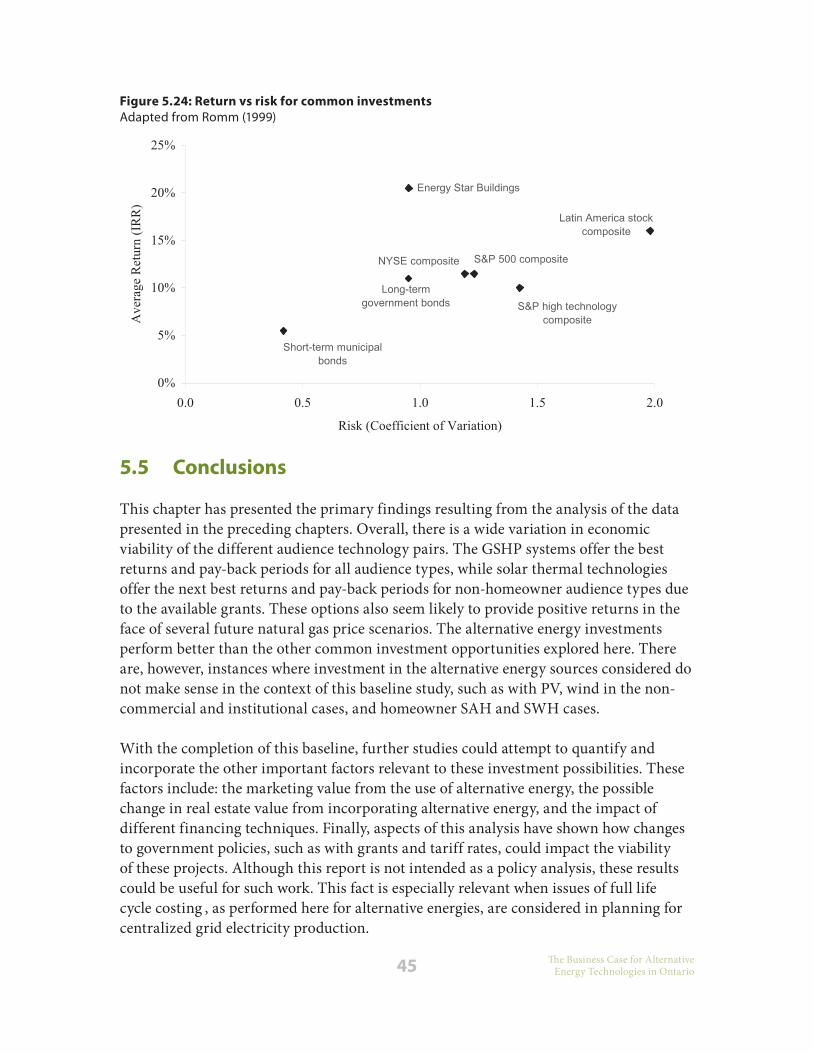
45 The Business Case for Alternative Energy Technologies in Ontario
5.5 Conclusions
This chapter has presented the primary findings resulting from the analysis of the data presented in the preceding chapters. Overall, there is a wide variation in economic viability of the different audience technology pairs. The GSHP systems offer the best returns and pay-back periods for all audience types, while solar thermal technologies offer the next best returns and pay-back periods for non-homeowner audience types due to the available grants. These options also seem likely to provide positive returns in the face of several future natural gas price scenarios. The alternative energy investments perform better than the other common investment opportunities explored here. There are, however, instances where investment in the alternative energy sources considered do not make sense in the context of this baseline study, such as with PV, wind in the non-commercial and institutional cases, and homeowner SAH and SWH cases.
With the completion of this baseline, further studies could attempt to quantify and incorporate the other important factors relevant to these investment possibilities. These factors include: the marketing value from the use of alternative energy, the possible change in real estate value from incorporating alternative energy, and the impact of different financing techniques. Finally, aspects of this analysis have shown how changes to government policies, such as with grants and tariff rates, could impact the viability of these projects. Although this report is not intended as a policy analysis, these results could be useful for such work. This fact is especially relevant when issues of full life cycle costing , as performed here for alternative energies, are considered in planning for centralized grid electricity production.
Figure 5.24: Return vs risk for common investmentsAdapted.from.Romm.(1999)

4�The Business Case for Alternative Energy Technologies in Ontario
References
Chapter 1:
NRCan, 2006a. RETScreen International. Accessed October 2007. <http://retscreen.net>
Romm, J.J. (1999) “Cool Companies: How the Best Businesses Boost Profits and Productivity by Cutting Greenhouse Gas Emissions,” Island Press.
Chapter 2: Energy Scenarios
Alberta Government, 2008. “Quantification Protocol for Solar Electricity Generation,” Accessed September 2008. <http://environment.gov.ab.ca/info/library/7958.pdf>
Environment Canada, 2003. “Canadian Wind Energy Atlas,” Accessed May 2008. <http://www.windatlas.ca/en/maps.php>
Environment Canada, 2008a. “Canada’s Offset System for Greenhouse Gases: Guide for Protocol Developers,” Accessed September 2008. <http://www.ec.gc.ca/creditscompensatoires-offsets/7CAD67C6-B798-4B69-9648-BD7F1F74B2CB/DRAFT%20Guide_for_Protocol_Developers.pdf>
Etcheverry, J., 2004. Smart Generation: Powering Ontario with Renewable Energy. David Suzuki Foundation. Accessed November 2007. <www.davidsuzuki.org/files/Climate/Ontario/Smart_Generation_full_report.pdf>
Hargreaves, P., 2008. Mondial Energy. Personal Communication.
NRCan, 2000. “Heating and Cooling with a Heat Pump,” Her Majesty the Queen in the Right of Canada.
NRCan, 2002. “Commercial Earth Energy Systems: A Buyer’s Guide,” Her Majesty the Queen in the Right of Canada.
NRCan, 2004. “Commercial & Institution Consumption of Energy Survey,” Her Majesty the Queen in the Right of Canada. Accessed June 2008. <http://oee.nrcan.gc.ca/Publications/statistics/cices05/pdf/cices05.pdf>
OPA (Ontario Power Authority), 2007. Integrated Power Systems Plan. Accessed January 2008. <http://www.powerauthority.on.ca/Page.asp?PageID=924&SiteNodeID=320>
4� The Business Case for Alternative Energy Technologies in Ontario
Skystream, 2008. “Skystream Specifications,” Accessed April 2008. <www.windenergy.com/documents/spec_sheets/3-CMLT-1338-01_Skystream_ spec.pdf>
TREC, 2007. Feasibility Analysis for a SolarShare Co-operative in the City of Toronto. Accessed Frebruary 2008. <http://www.trec.on.ca/documents/SolarShare%20TAF%20Report.PDF>
UNFCC (United Nations Framework Convention on Climate Change), 2006. “Consolidated baseline methodology for grid-connected electricity generation from renewable sources – Version 6,” Accessed September 2008. <http://cdm.unfccc.int/UserManagement/FileStorage/CDMWF_AM_BW759ID58ST5YEEV6WUCN5744MN763>
UNFCC (United Nations Framework Convention on Climate Change), 2008. “Tool to calculate the emission factor for an electricity system,” Accessed September 2008. <http://cdm.unfccc.int/methodologies/Tools/EB35_repan12_Tool_grid_ emission.pdf>
Chapter 3: System Costs
Ayoub, J., 2006. “National Survey Report of PV Power Applications in Canada,” Accessed November 2007. <http://www.cansia.ca/downloads/NationalStatusReport2006.pdf>
Bailie, A., Horne, M., Peters, R., Taylor, A., Weis, T., Cobb, P., Zarowny, K., 2007. “Economic Instruments for On-site Renewable Energy Applications in the Residential/Farm Sector,” Pembina Institute. Accessed May 2008. <http://pubs.pembina.org/reports/Econ_Instru_Res_RE_03-07.pdf>
Cane, D., Garnet, J.M., 2000. Update on Maintenance and Service Costs of Commercial Building Ground-Source Heat Pump Systems. ASHRAE Transactions, vol 106, pg 399-407.
CanSIA, 2005. The Potential of Solar PV in Ontario. Accessed May 2008. <http://www.cansia.ca/downloads/report2005/C18.pdf>
Fraser, N.M., Bernhardt, I., Jewkes, E.M., Tajima, M., 2000. Engineering Economics in Canada. Second Edition. Prentice Hall Canada, Scarborough, Ontario.
Government of Canada, 2008a. “ecoEnergy for renewable Heat: Deployment Incentive Terms and Conditions,” Accessed May 2008. <www.ecoaction.gc.ca/ecoenergy-ecoenergie/heat-chauffage/conditions-eng.cfm>

4�The Business Case for Alternative Energy Technologies in Ontario
Government of Canada, 2008b. “ecoEnergy: Ontario Solar Thermal Incentive Program (OSTHI),” Accessed May 2008. <www.ecoaction.gc.ca/ecoenergy-ecoenergie/heat-chauffage/on-osthi-ioscst-eng.cfm>
Government of Ontario, 2007, “Heating and Cooling your Home, Chapter 13,” Ministry of Energy and Infrastructure. Accessed July 2008. <http://www.energy.gov.on.ca/index.cfm?fuseaction=conservation.guide13>
Kapoor, A. 2008. REDI System Costs, NRCan. Personal Communication.
Marbek Resource Consultants Ltd., 2005. Survey of the Small (300 W to 300 kW) Wind Turbine Market in Canada. Ottawa, Ontario, Canada.
Schafer, 2008. Region of Peel. Personal Communication.
Traynor, K., 2008. Ourpower.ca. Personal Communication.
Chapter 4: Energy Price Projections
Budzik, P., 2003. “U.S. Natural Gas Markets: Relationship Between Henry Hub Spot Prices and U.S. Wellhead Prices,” Accessed August 2008. <http://www.eia.doe.gov/oiaf/analysispaper/henryhub/pdf/henryhub.pdf>
EIA (Energy Information Administration), 2007. “Annual Energy Outlook 2007,” Accessed April 2008. <http://www.eia.doe.gov/oiaf/aeo/pdf/0383(2008).pdf>
Enbridge, 2007. “Fall 2007 Consensus Natural Gas Commodity Forecast”
Greenpeace, EREC (European Renewable Energy Council), 2007. “Energy [r]evolution: A Sustainable World Energy Outlook,” Accessed April 2007. <http://www.energyblueprint.info/fileadmin/media/documents/energy_revolution.pdf>
IEA. 2004. “IEA World Energy Outlook 2004.” Copyright OECD/IEA.
NEB (National Energy Board), 2007. “Canada’s Energy Future: Reference Case & Scenarios to 2030,” Accessed April 2008. <http://www.neb.gc.ca/clf-nsi/rnrgynfmtn/nrgyrprt/nrgyftr/2007/nrgyftr2007-eng.pdf>
NPC (National Petroleum Council), 2007. “Hard Truths: Facing the Hard Truths about Energy.”

4� The Business Case for Alternative Energy Technologies in Ontario
NRCan, 2006b. “Canada’s Energy Outlook: The Reference Case 2006,” Accessed April 2008. <http://www.nrcan.gc.ca/com/resoress/publications/peo/peo2006-eng.pdf>
Sproule, 2008. “Sproule Prices and Market Forecasts,” Accessed July 2008. <http://www.sproule.com/prices/defaultprices.htm>
OEB (Ontario Energy Board), 2008. “2008 Decisions and Reports,” Accessed June 2008. <http://www.oeb.gov.on.ca/OEB/Hearings+and+Decisions/Decisions+and+Reports>
OPA (Ontario Power Authority), 2007. “Integrated Power Systems Plan,” Accessed April 2008. <http://www.powerauthority.on.ca/Page.asp?PageID=1224&SiteNodeID=320>
Chapter 5: Business Case
Environment Canada, 2008b. “Turning the Corner: Detailed Emissions and Economic Modeling,” Accessed September 2008. <http://www.ec.gc.ca/doc/virage-corner/2008-03/571/tdm_toc_eng.htm>
Darley, J. 2004. High Noon for Natural Gas: The New Energy Crisis. White River Junction, Vermont: Chelsea Green Publishing Company
Deffeyes, K.S. 2005. Beyond Oil: The View from Hubbert’s Peak. New York, NY: Hill and Wang.
Heinberg, R. 2005. The Party’s Over: Oil, War and the Fate of Industrial Societies. Gabriola Island, BC: New Society Publishers.
Hubbert Peak, 2007. The Hubbert Peak of World Oil. Accessed April 2008. <http://www.hubbertpeak.com/summary.htm>

50The Business Case for Alternative Energy Technologies in Ontario
Appendices
A) Environmental Parameters
The below data describes the local details used for the study.1
Unit Climate data Project location
Latitude ˚N 43.7
Longitude ˚E -79.4
Elevation m 107
Heating.design.temperature °C -17.1
Cooling.design.temperature °C 28.8
Earth.temperature.amplitude °C 21.3
The following summarizes the environmental and weather conditions used for the study (data from measurements at 10 metres).¹
Mon
th
Air
tem
pera
ture
(°C)
Rela
tive
hum
idit
y(%
)
Dai
ly s
olar
radi
atio
n –
hori
zont
al (k
Wh/
m²/d
)
Atm
osph
eric
pre
ssur
e (k
Pa)
Win
d sp
eed
(m/s
)
Eart
h te
mpe
ratu
re
(°C)
hea
ting
deg
ree-
days
(°
C-d)
Cool
ing
degr
ee-d
ays
(°C-
d)
Jan -7.1 79% 1.44 99.5 4.7 -7.6 778 0
Feb -6.2 77% 2.22 99.5 4.4 -5.9 678 0
Mar -0.8 76% 3.36 99.5 4.5 -0.1 583 0
Apr 6.3 69% 4.5 99.3 4.4 7.4 351 0
May 12.4 68% 5.47 99.4 3.7 13.8 174 74
Jun 17.4 70% 6 99.3 3.4 18.7 18 222
Jul 20.5 70% 6.14 99.4 3.3 20.9 0 326
Aug 19.5 73% 5.14 99.5 3.3 19.5 0 295
Sep 15.2 75% 3.75 99.6 3.8 15.1 84 156
Oct 8.9 76% 2.47 99.6 4.3 8.8 282 0
Nov 3.1 80% 1.31 99.5 4.8 2.6 447 0
Dec -3.2 81% 1 99.5 4.8 -4.3 657 0
Yearly 7.24 74% 3.57 99.5 4.1 7.5 4052 1073
1 RETScreen (see www.retscreen.net for more information).

51 The Business Case for Alternative Energy Technologies in Ontario
B) REDI Data
The data presented here are from the experience gained from the national Renewable Energy Deployment Initiative (REDI)2 and are used in the study to price SAH and SWH systems.
SAh installed costs from REDI program 1���–200�
2 Kapoor, A. 2008. REDI System Costs, NRCan. Personal Communication.
SAh installed system characteristics from REDI 1���–200� (Kapoor, 200�)
Year Fiscal year No. of systems
Collector area (m2)
System costs ($)
($/m2)
1 1998–1999 . 5 . 2,180 . $452,613. . 207.62
2 1999–2000 . 3 . 1,690 . $403,190. . 238.57
3 2000–2001 . 6 . 1,127 . $461,989. . 409.92
4 2001–2002 . 19 . 3,488 . $1,396,633. . 400.41
5 2002–2003 . 26 . 4,319 . $1,763,737. . 408.36
6 2003–2004 . 61 . 14,018 . $5,671,247. . 404.56
7 2004–2005 . 33 . 7,462 . $2,987,273. . 400.33
8 2005–2006 . 60 . 13,597 . $6,302,702. . 463.53
9 2006–2007 . 69 . 17,675 . $6,443,442. . 364.55
TOTAL -- . 2�2 . �5,55� . $25,��2,�2� . 3�4.�2

52The Business Case for Alternative Energy Technologies in Ontario
SWh Sample of solar water glazed systems: costs and collector area
Sample SWh REDI installation characteristics from 1���–200�
Technology No. of systems Average collector area per system
(m2)
Average cost per m2 ($)
R2
Glazed . 78 . 44.95 . $1,032.73. 0.84
Unglazed . 27 . 143.71 . $197.60. 0.77
ETC . 10 . 37.75 . $1,374.80. Unavailable
Totals . 115 . 67.51 . $631.99. --

53 The Business Case for Alternative Energy Technologies in Ontario

54The Business Case for Alternative Energy Technologies in Ontario
