the c-band all-sky survey (c-bass): constraining di use ... · valley radio observatory,...

Mon. Not. R. Astron. Soc. 000, 1–19 (2014) Printed 21 February 2019 (MN LATEX style file v2.2)

The C-Band All-Sky Survey (C-BASS): Constrainingdiffuse Galactic radio emission in the North Celestial Poleregion

C. Dickinson,1,2? A. Barr,1 H. C. Chiang,3,4 C. Copley,5,6,7 R. D. P. Grumitt,7

S. E. Harper,1 H. M. Heilgendorff,4 L. R. P. Jew,7 J. L. Jonas,5,6 Michael E. Jones,7

J. P. Leahy,1 J. Leech,7 E. M. Leitch,2 S. J. C. Muchovej,2 T. J. Pearson,2 M. W. Peel,8,1

A. C. S. Readhead,2 J. Sievers,3,9 M. A. Stevenson,2 Angela C. Taylor,71Jodrell Bank Centre for Astrophysics, Alan Turing building, School of Physics and Astronomy, The University of Manchester,

Oxford Road, Manchester, M13 9PL, Manchester, U.K.2Cahill Centre for Astronomy and Astrophysics, California Institute of Technology, Pasadena, CA 91125, USA3Department of Physics, McGill University, 3600 Rue University, Montreal, QC H3A 2T8, Canada4Astrophysics & Cosmology Research Unit, School of Mathematics, Statistics & Computer Science, University of KwaZulu-Natal,Westville Campus, Private Bag X54001, Durban 4000, South Africa5Department of Physics and Electronics, Rhodes University, Grahamstown, 6139, South Africa6South African Radio Astronomy Observatory, 2 Fir Road, Observatory, Cape Town, 7925 , South Africa7Sub-department of Astrophysics, University of Oxford, Denys Wilkinson Building, Keble Road, Oxford OX1 3RH, U.K.8Departamento de Fısica Matematica, Instituto de Fısica, Universidade de Sao Paulo, Rua do Matao 1371, Sao Paulo, Brazil9School of Chemistry and Physics, University of KwaZulu-Natal, Westville Campus, Private Bag X54001, Durban 4000, South Africa

Accepted XXX. Received YYY; in original form ZZZ

ABSTRACTThe C-Band All-Sky Survey (C-BASS) is a high-sensitivity all-sky radio survey at anangular resolution of 45 arcmin and a frequency of 4.7 GHz. We present a total inten-sity map of the North Celestial Pole (NCP) region of sky, above declination > +80◦,which is limited by source confusion at a level of ≈ 0.6 mK rms. We apply the template-fitting (cross-correlation) technique to WMAP and Planck data, using the C-BASSmap as the synchrotron template, to investigate the contribution of diffuse foregroundemission at frequencies ∼ 20–40 GHz. We quantify the anomalous microwave emission(AME) that is correlated with far-infrared dust emission. The AME amplitude doesnot change significantly (< 10 %) when using the higher frequency C-BASS 4.7 GHztemplate instead of the traditional Haslam 408 MHz map as a tracer of synchrotron ra-diation. We measure template coefficients of 9.93±0.35 and 9.52±0.34 K per unit τ353when using the Haslam and C-BASS synchrotron templates, respectively. The AMEcontributes 55±2µK rms at 22.8 GHz and accounts for ≈ 60% of the total foregroundemission. Our results show that a harder (flatter spectrum) component of synchrotronemission is not dominant at frequencies & 5 GHz; the best-fitting synchrotron temper-ature spectral index is β = −2.91 ± 0.04 from 4.7 to 22.8 GHz and β = −2.85 ± 0.14from 22.8 to 44.1 GHz. Free-free emission is weak, contributing ≈ 7µK rms (≈ 7%)at 22.8 GHz. The best explanation for the AME is still electric dipole emission fromsmall spinning dust grains.

Key words: surveys – radiation mechanism: non-thermal – radiation mechanism:thermal – diffuse radiation – radio continuum: ISM.

? E-mail:[email protected]

1 INTRODUCTION

Diffuse radio foreground emission is a useful tool for study-ing the various components of the interstellar medium(ISM), including cosmic ray electrons via synchrotron ra-diation (Lawson et al. 1987; Strong, Orlando & Jaffe 2011;

c© 2014 RAS

arX

iv:1

810.

1168

1v2

[as

tro-

ph.G

A]

19

Feb

2019

E-mail: [email protected]

2 C. Dickinson et al.

Orlando & Strong 2013) and warm ionized medium (WIM)via free-free emission (Davies et al. 2006; Jaffe et al. 2011;Planck Collaboration et al. 2011a; Alves et al. 2012). Under-standing their detailed spatial and spectral characteristicsis also important for removing them from cosmic microwavebackground (CMB) data (Leach et al. 2008; Dunkley et al.2009a; Delabrouille & Cardoso 2009; Armitage-Caplan et al.2012; Errard & Stompor 2012; Planck Collaboration et al.2013a, 2016b; Remazeilles et al. 2016).

An additional component, referred to as Anomalous Mi-crowave Emission (AME), has been detected at frequencies∼10–60 GHz (Kogut et al. 1996; Leitch et al. 1997; Ban-day et al. 2003; Lagache 2003; de Oliveira-Costa et al. 2004;Davies et al. 2006; Kogut et al. 2011; Gold et al. 2011; Ghoshet al. 2012); see Dickinson et al. (2018) for a recent review.This emission does not appear to correlate with low radiofrequency data, such as the 408 MHz map by Haslam et al.(1982), which rules out steep-spectrum synchrotron emis-sion as a cause. Similarly, analyses have shown that AMEdoes not strongly correlate with Hα data (e.g., Dickinson,Davies & Davis 2003; Finkbeiner 2003), which rules out free-free emission from warm (Te ≈ 104 K) ionized gas. However,AME is remarkably well-correlated with far-infrared (FIR)and sub-mm maps (Leitch et al. 1997; Miville-Deschenes &Lagache 2005) which trace interstellar dust grains in theISM. Draine & Lazarian (1998a) revisited the theory of elec-tric dipole radiation from small spinning dust grains (“spin-ning dust”), originally postulated by Erickson (1957), andshowed that spinning dust can naturally account for AMEand explain the close correlation with FIR emission. Sincethen, there has been considerable evidence for spinning dustemission from molecular clouds and Hii regions (Finkbeineret al. 2002; Casassus et al. 2006, 2008; Dickinson et al.2009, 2010; Scaife et al. 2009). The best examples are diffuseclouds within the Perseus (Watson et al. 2005) and ρ Ophi-uchi (Casassus et al. 2008) regions, which have high precisionspectra showing the characteristic “bump” (in flux density)at a frequency of ≈ 30 GHz and can be fitted by plausiblephysical models for the spinning dust grains (Planck Collab-oration et al. 2011b; Tibbs et al. 2011). A survey of brightGalactic clouds in the Planck data (Planck Collaborationet al. 2014c) has detected a number of potential candidatesbut follow-up observations at higher resolution are requiredto confirm them.

The origin of the diffuse AME found at high Galacticlatitudes is still not clear (e.g., Hensley, Draine & Meisner2016). Although spinning dust can readily account for thebulk of the AME (e.g., Planck Collaboration et al. 2016a),other emission mechanisms could be contributing (PlanckCollaboration et al. 2016c). Magnetic dipole radiation fromfluctuations in dust grain magnetization could be significant(Draine & Lazarian 1999; Draine & Hensley 2013; Hensley,Draine & Meisner 2016; Hoang & Lazarian 2016), althoughupper limits on AME polarization (Lopez-Caraballo et al.2011; Dickinson, Peel & Vidal 2011; Macellari et al. 2011;Rubino-Martın et al. 2012; Genova-Santos et al. 2017) ap-pear to indicate that this cannot account for the majorityof the signal. Similarly, a harder (flatter spectrum) compo-nent of synchrotron radiation may also be responsible forAME, which was proposed by Bennett et al. (2003) at thetime of the first WMAP data release. The harder spectrumnaturally explains the correlation with dust, since both are

related to the process of star-formation. Furthermore, wealready know that there are regions that have synchrotronspectral indices1 that are at β ≈ −2.5 or flatter, both super-nova remnants (Onic 2013) and more diffuse regions such asthe WMAP/Planck haze (Finkbeiner 2004; Planck Collabo-ration et al. 2013b).

A harder synchrotron component may have been missedwhen applying component separation methods to microwavedata. The majority of AME detections from fluctuations athigh Galactic latitudes have been made using the “tem-plate fitting” technique, i.e., fitting multiple templates foreach foreground component to CMB data, accounting forCMB fluctuations and noise (Kogut et al. 1996; Bandayet al. 2003). The synchrotron template is traditionally the408 MHz all-sky map (Haslam et al. 1982), or another lowfrequency template. However, data at these frequencies willnaturally be sensitive to the softer (steeper spectrum) syn-chrotron emission, which has a temperature spectral index(T ∝ νβ) β ≈ −3.0 at frequencies & 5 GHz (Davies, Wat-son & Gutierrez 1996; Davies et al. 2006; Kogut et al. 2007;Dunkley et al. 2009b; Gold et al. 2011). This leads to a signif-icant AME signal at ∼10–60 GHz that is correlated with FIRtemplates, which cannot be accounted for by the Rayleigh-Jeans tail of dust emission.

A hard synchrotron component of AME can be con-strained (or ruled out) by using a higher radio frequencytemplate of synchrotron emission. Peel et al. (2012) usedthe 2.3 GHz southern-sky survey of Jonas, Baart & Nicolson(1998) as a synchrotron template for the WMAP data andfound that the dust-correlated AME component changed byonly ≈ 7 %, compared to using the 408 MHz template. Thissuggests that the the bulk of the diffuse high latitude syn-chrotron emission is indeed steep (β ≈ −3.0) above 2.3 GHz,resulting in little change to the AME at 20–40 GHz.

The C-Band All-Sky Survey (C-BASS) is a survey ofthe entire sky at 5 GHz, in intensity and polarization, at aresolution of 45 arcmin (King et al. 2010; Jones et al. 2018).The frequency chosen is ideal for CMB component separa-tion studies, being much closer to observing frequencies usedby CMB experiments, typically at 30 GHz and higher. Thenorthern survey (King et al. 2014) observations are completeand will be described in forthcoming papers. First resultsfrom the bright Galactic plane emission have been presentedby Irfan et al. (2015).

In this paper we present a preliminary C-BASS inten-sity map at 5 GHz of the North Celestial Pole (NCP) region,primarily based on the joint-fitting of spatial templates at agiven frequency (e.g., Davies et al. 2006). The NCP area isknown to have significant AME and FIR emission from thePolaris flare region, sometimes known as “the duck” (Davieset al. 2006), having been studied in the first identificationof AME (Leitch et al. 1997). The AME is relatively bright,while the synchrotron and free-free components appear to beweak, and their morphology is distinct from the AME/FIRemission. Furthermore, the older surveys of Haslam et al.(1982) at 408 MHz and Reich & Reich (1986) at 1.4 GHzare clearly affected by varying zero-levels, which appear as

1 We use brightness temperature spectral indices, given by thedefinition Tb ∝ νβ , which are related to flux density spectral

indices by α = β + 2.

c© 2014 RAS, MNRAS 000, 1–19

C-BASS: Constraining diffuse radio emission in the NCP region 3

stripes in these maps. Also, due to the C-BASS scan strat-egy, the NCP region is observed very deeply by the C-BASSnorthern telescope, and has an almost negligible level of in-strumental noise.

Section 2 describes the C-BASS observations and dataanalysis. Maps are presented in Section 3. The template-fitting results and foreground spectral energy distributions(SEDs) are presented in Section 4. A discussion of the resultsfor each component is given in Section 5. Conclusions aresummarized in Section 6.

2 OBSERVATIONS AND DATA ANALYSIS

The C-BASS project is surveying the entire sky, in intensityand polarization, at a nominal frequency of 5 GHz and anangular resolution of ≈ 45 arcmin (Jones et al. 2018). It usestwo telescopes to obtain full-sky coverage; the northern tele-scope is a 6.1 m Gregorian antenna situated at the OwensValley Radio Observatory, California, and the southern tele-scope is a 7.6 m Cassegrain antenna situated at Klerefontein,the MeerKAT/SKA South Africa support base. The north-ern instrument was commissioned in 2009–2012 (Muchovejet al., in prep.) and observed routinely until 2015 April, af-ter which the receiver was decommissioned. The southerninstrument is currently carrying out the southern part ofthe survey.

2.1 Observations

The C-BASS scan strategy consists of 360◦ scans in azimuthat a constant elevation, at a speed of ≈ 4◦ azimuth per sec-ond. The majority of the northern survey data were takenat elevations of 37.◦2 (therefore passing through the NCP)and 47.◦2, with additional scans at 67.◦2 and 77.◦2 to im-prove coverage at intermediate declinations. For the NCPregion, only data at the two lower elevations are relevant,since higher elevations do not pass through the NCP region.However, the higher elevation data are useful in reducingthe effects of drifts in the data due to 1/f noise (Taylor etal., in prep.).

The C-BASS receiver is a continuous-comparison ra-diometer (King et al. 2014), which measures the differencebetween sky brightness temperature and a stabilised resis-tive load. This architecture reduces receiver 1/f noise, whichwould otherwise be indistinguishable from variations on thesky. The receiver also implements a correlation polarimeter.However, no polarization data are used in this present analy-sis. In this paper we use data taken from the C-BASS Northsurvey, covering the period 2012 November to 2015 March.

2.2 Data analysis

The data have been processed using the latest version of thestandard C-BASS data reduction pipeline. A detailed de-scription of the pipeline will be given in forthcoming papers.In brief, the reduction pipeline identifies and flags out eventsof radio frequency interference, performs amplitude and po-larization calibration, and applies atmospheric opacity cor-rections. It also removes contamination due to microphonicscaused by the cryocooler cycle, which introduce oscillations

in the output signal at a frequency of 1.2 Hz and harmon-ics thereof. Residual 1.2 Hz contamination is estimated tobe at a level comparable to the thermal noise. The pipelinealso removes large-scale ground spillover. Ground templatesare made for each day of observations by subtracting thecurrent best sky model from the time-ordered data, mask-ing the strongest regions of Galactic emission, and binningin azimuth. This azimuth template is then subtracted fromthe time-ordered data before mapping. As well as removingthe majority of the ground emission, this process inevitablyremoves a small fraction of the right-ascension-averaged skysignal. This is a significant effect on large angular scales butis not expected to be a major issue in the small region atthe NCP analysed here. This effect will be mitigated in fu-ture analyses by including data from the southern survey,which have very different ground contamination at a givensky position. The current analysis also uses data taken onlywhen the Sun is below the horizon, and all data within 5◦

of the Moon are also flagged.

The northern receiver includes a noise diode which,when fired, injects a signal of constant temperature. Thepipeline calibrates the intensity signal onto the noise diodescale, and the noise diode is subsequently calibrated to theastronomical sources Cas A and Tau A. The calibrator fluxdensities are calculated from the spectral forms given in Wei-land et al. (2011). The noise diode temperature is stable towithin 1 per cent over time periods of several months and at-mospheric opacity corrections are typically < 1 %, resultingin relative calibration uncertainties of ≈ 1 % (Irfan 2014).

The northern receiver has a nominal bandpass of 4.5–5.5 GHz but in-band filters to remove terrestrial RFI re-duce the effective bandwidth to 0.499 GHz with a centralfrequency of 4.783 GHz. The effective observing frequencydepends on the calibrator source and the source spectrumbeing observed but we do not attempt to colour correct thedata considered in this paper as these corrections are of order1 per cent. Since our main calibrator is Tau A (β = −2.3),and the bulk of the emission seen by C-BASS is steeper-spectrum synchrotron (β ≈ −3), the effective frequency willbe slightly lower than this by ≈ 0.05–0.1 GHz. We thereforeassume an effective frequency of 4.7 GHz throughout thispaper.

The initial absolute calibration of the C-BASS mapsis computed in terms of antenna temperature, which corre-sponds to the sky convolved with the full C-BASS beam.Since there is a significant (≈ 25 %; Holler et al. 2013)amount of power outside of the main beam, the conversionto brightness temperature depends on the angular scale ofinterest. In previous work, a common way around this issuehas been to correct the scale to the “main beam” (pointsource) or “full beam” (extended source) scale to accountfor power lost to the far sidelobes (e.g., Reich 1982; Jonas,Baart & Nicolson 1998). For a previous C-BASS paper (Ir-fan et al. 2015), we used a single factor of 1.124 to convert toan effective full-beam temperature scale for angular scalesof a few degrees.

For the analysis in this paper, we use the theoreticalbeam calculated using the GRASP physical optics pack-age (Holler et al. 2013) to deconvolve the sidelobe responsewhile smoothing to an effective Gaussian resolution of 1◦

full width at half maximum (FWHM). This produces mapswith the correct resolution and smoothing function and it

c© 2014 RAS, MNRAS 000, 1–19


also results in a brightness temperature scale that is not de-pendent on angular scale. We find that the flux densities ofbright sources agree with previous measurements to within≈ 5 %. Since in this analysis we do not take into accountthe effects of a finite bandpass (colour corrections), we willadopt 5 % as our absolute calibration uncertainty. With fu-ture C-BASS data releases, and taking into account colourcorrections, we expect to be able to reach ≈ 1 % accuracy.

The C-BASS maps are made by the DEStriping CAR-Tographer, Descart (Sutton et al. 2010). Descart per-forms a maximum likelihood fit to the contribution of 1/fnoise in our timestreams with a series of offsets to the sig-nal baseline, in this case 5 s long. Different scans are giventhe same optimal σ−2 weighting as is used in full maximumlikelihood mapping, and are treated as independent. Vari-ances were estimated from the power spectrum of the data.White-noise correlation between the channels is neglectedfor this work. The C-BASS data are made into HEALPix

(Gorski et al. 2005)2 maps at Nside = 256, correspondingto pixels ≈ 13.4 arcmin on-a-side.

3 MAPS

3.1 C-BASS NCP map

The unsmoothed C-BASS 5 GHz map of the NCP region isshown in the top panel of Fig. 1. The image is a gnomonicprojection of the HEALPix Nside = 256 map, in units ofmK (Rayleigh-Jeans), and with an angular resolution of45 arcmin FWHM. An approximate zero level has been re-moved by subtracting the global minimum in the map toensure positivity; the results are insensitive to this globaloffset. The map contains hundreds of radio sources super-posed onto diffuse Galactic emission; sources brighter than200 mJy at 4.85 GHz and at δ > +75◦ are marked with smallcircles. The majority of the radio sources are extragalacticand will be discussed further in Section 3.2. The diffuse emis-sion is expected to be primarily synchrotron radiation, witha contribution of free-free emission from our Galaxy. TheGalactic plane is located towards the bottom of the mapwhere the brightest emission is located.

The integration time for each Nside = 256 (≈13.4 arcmin on-a-side) pixel is shown in the lower panelof Fig. 1. The integration time in the NCP region is veryhigh everywhere due to the constant elevation scans thatrepeatedly cross the NCP region. The median integrationat δ > +80◦ is 50 s per Nside = 256 pixel, and much higherin the centre of the map. For the analyses at Nside = 64(≈ 55.0 arcmin pixels), the integration time is effectively 16times this value, i.e., ≈ 800 s. For the typical C-BASS rmsnoise level of ≈ 2.0 mK s1/2 in intensity, this corresponds toa map rms noise level of ≈ 0.07 mK or better. Compared tothe Galactic signal of several mK, the instrumental noise istherefore effectively negligible in this region. The typical rmsconfusion noise from fluctuations in the background of radiosources at this angular resolution is ∼ 0.6 mK (Jones et al.2018). The effects of a large number of weak sources canbe seen in the colder regions of the C-BASS map (Fig. 1).

2 http://healpix.sourceforge.net

Figure 1. Top: Unsmoothed C-BASS 5 GHz Nside = 256 map

of the NCP region at an angular resolution of 45 arcmin FWHM.

The map covers a 30◦×30◦ region centred at the NCP (δ = +90◦)with R.A.=0◦ at the bottom of the map (R.A.=180◦ at the top)and increasing clockwise. The circular graticule lines mark 5◦ in-

tervals in declination. The colour scale is linear between the min-imum/maximum values shown. Radio sources with flux densities

> 200 mJy and δ > +75◦ from the Mingaliev et al. (2007) cata-

logue are indicated by circles, with larger circles for flux densities> 600 mJy. Bottom: Map of integration time (sec) perNside = 256

pixel on a logarithmic scale. The NCP region has the deepest inte-

gration in the C-BASS data. The circular rings correspond to thehigher declination limits where the telescope is turning around,

resulting in higher hit counts.

c© 2014 RAS, MNRAS 000, 1–19

http://healpix.sourceforge.net


Bright (& 200 mJy) extragalactic sources will be removedfrom the C-BASS map before analysis (see Sect. 3.2).

The analysis was repeated on several versions of theC-BASS map, using a variety of data cuts and analysis pro-cedures. Visual inspection of the maps showed the samestructures at the same intensity level. Difference maps re-vealed low-level artifacts that were typically a few per centor less of the signal of interest. The main contaminant wasthe Sun (via the far-out sidelobes of the C-BASS beam),which produced large-scale emission and scatter across themap, comparable to the Galactic emission in the NCP re-gion. We therefore chose to use night-time only data, wherethis effect was eliminated. Nevertheless, we found that theresults were consistent within the quoted uncertainties.

3.2 Extragalactic radio sources in the NCP region

It is clear that there is a significant contribution from ex-tragalactic sources in the C-BASS data. The large beam ofC-BASS means that the point-source flux density sensitiv-ity is modest and we are limited by source confusion. Thebrightest sources are easily discernible in the C-BASS map(Fig. 1). Fortunately, a number of high angular resolutionradio surveys have been made of the region, and they canbe used to either mask or remove the brightest sources.

The Kuhr et al. (1981a) S5 survey mapped the NCPregion (δ > +70◦) with the Effelsberg 100-m telescope, with476 detected sources, and is complete down to 250 mJy. Un-fortunately, an electronic version of this catalogue is notcurrently available. The Kuhr et al. (1981b) 5 GHz cata-logue of bright (> 1 Jy) sources contains only 7 sources atδ > +80◦. The Green Bank 6-cm radio source catalog (Gre-gory et al. 1996) is a blind survey complete to ≈ 18 mJy butis limited to δ < +75◦ and therefore is not useful here. TheNRAO VLA All-Sky Survey (NVSS; Condon et al. 1998)at 1.4 GHz is the highest frequency unbiased radio surveythat covers δ > +88◦; it contains hundreds of radio sourcesbut the majority are ∼ 3–100 mJy and cannot be accuratelyextrapolated to 5 GHz. Healey et al. (2009) surveyed theregion at 4.85 GHz but pre-selected sources that were flatspectrum. They measured 3 sources in this relatively unob-served region (δ > +88◦) at 4.85 GHz with flux densities of67, 58 and 142 mJy, respectively. Ricci et al. (2013) made5–30 GHz measurements of bright sources detected in theK-band Medicina pilot survey (Righini et al. 2012).

The only other radio survey of the NCP region (δ >+75◦) at frequencies above 1.4 GHz is the RATAN-600multi-frequency survey of Mingaliev et al. (2007), which in-cludes measurements at 4.8 GHz. They observed 504 sourcesfrom the 1.4 GHz NVSS that were located +75◦ < δ < +88◦

and had a flux density S1.4GHz > 0.2 Jy. We therefore usethe 4.8 GHz catalogue of Mingaliev et al. (2007) for identi-fying and masking sources in the NCP region.

The locations of radio sources above 200 mJy from Min-galiev et al. (2007) are over-plotted in Fig. 1. The brightestsources (> 600 mJy) at δ > +80◦ are listed in Table 1. Vir-tually all of these sources at δ > +75◦ lie on peaks in theC-BASS map. This is reassuring and indicates that we un-derstand well the bright source population at 5 GHz. How-ever, it should be noted that a number of these sources ex-hibit variability in their flux density (e.g., Liu et al. 2014).The brightest source in our field (δ > +80◦) away is the

double-lobed radio galaxy 3C 61.1, which has a flux densityof ≈ 2 Jy at 4.7 GHz (Hargrave & McEllin 1975).3

Fig. 2 shows the map of point sources, convolved witha 1◦ FWHM Gaussian beam. The fluctuations in bright-ness temperature are at the level of ≈ 1–2 mK away frombright sources. The source 3C 61.1 has a peak brightnesstemperature of ≈ 9 mK above the background. In the mid-dle panel of Fig. 2 we show the C-BASS map after smooth-ing (and deconvolving) to the common 1◦ FWHM resolu-tion. The right panel shows the C-BASS map after sub-tracting the map of sources. Visual inspection shows thatthe subtraction has been successful, with most of the ob-vious sources no longer being visible. For the brightest fewsources (3C 61.1, NGC 6251) the subtraction is not perfect.For example, NGC 6251 has been under-subtracted (possiblydue to its large angular extent of over 1◦). These could beremoved by fitting for their flux densities separately. How-ever, we choose to mask the four brightest sources with anaperture of 0.◦7 radius. We also mask out the NCP itself(δ = +90◦) because there appears to be a relatively brightsource in the C-BASS map, which is not in the majorityof source catalogues. The source mask is shown in Fig. 2.Fainter sources can be either masked or subtracted, as a testof point-source contamination. Our results are not stronglysensitive to the effects of residual source contamination (seeSect. 4.2).

At the higher frequencies (& 20 GHz) observed byWMAP and Planck, some of the weaker radio sources aremuch fainter than at lower frequencies because many galax-ies have spectral indices α < 0 (flux density S ∝ να). Themain population of radio sources at frequencies & 20 GHz,particularly at high flux densities, are galaxies that har-bour active galactic nuclei (AGN), which can produce flat-spectrum radiation up to tens of gigahertz or even higher.In the NCP region (δ > +75◦), the Planck compact sourcecatalogue, PCCS2 (Planck Collaboration et al. 2016d), con-tains 28 sources above 0.5 Jy while only 3 sources are above1 Jy. Of these, only 1 source (NGC 6251) is in the δ > +80◦

region, with a 28.4 GHz flux density of 1.3 ± 0.1 Jy. Pixelsaffected by this source will be masked out.

3.3 Multi-frequency maps of the NCP region at1◦ resolution

We now compare the C-BASS data with multi-frequencyradio, microwave and FIR data. The datasets are summa-rized in Table 2. The absolute calibration uncertainties arethose assumed later in the analysis. Data from WMAP 9-year (Bennett et al. 2013) and Planck 2018 results (PR3)(Planck Collaboration et al. 2018a) are the primary databeing analysed. We assume a conservative minimum 3 %

3 The Mingaliev et al. (2007) catalogue reports a flux density for

3C 61.1 of 970 ± 80 mJy at 4.8 GHz, which is inconsistent withvarious measurements of ≈ 1.9 Jy at 5 GHz (the source is not

thought to be significantly variable). Since they report 3 individ-ual sources (they do not give the flux densities for these due toconfusion of multiple sources hence the “X”s in the catalogue en-

try) it may be that this is a typographical error in which they havereported one of the contributing sources. Other sources appear tobe unaffected.

c© 2014 RAS, MNRAS 000, 1–19


Table 1. List of bright (> 600 mJy) sources in the NCP region (δ > +80◦), ordered in decreasing flux density. Flux densities at 4.8 GHz

are taken from Mingaliev et al. (2007), except for 3C 61.1∗ (see text and footnote3), which is taken from Hargrave & McEllin (1975).

The uncertainties are dominated by 3% calibration errors.

Source Flux density (R.A.,Dec.) [J2000] (l, b) Alternate name[mJy] [deg.] [deg.]

115312+805829 2130 (178.30,+80.97) (125.72,+35.84) S5 0014+810222XX+86XXXX∗ 1900 (35.70,+86.31) (124.49,+23.72) 3C 61.1

234403+822640 1433 (356.02,+82.44) (120.61,+19.88) S5 1150+81

104423+805439 1404 (161.10,+80.91) (128.74,+34.74) S5 1039+81001708+813508 1190 (4.29,+81.59) (121.61,+18.80) S5 0014+81

075058+824158 1061 (117.74,+82.70) (130.99,+28.77) S5 0740+82

074305+802544 804 (115.77,+80.43) (133.60,+28.86) 3C 184.1062602+820225 751 (96.51,+82.04) (131.74,+25.97) S5 0615+82

163226+823220 749 (248.11,+82.54) (115.77,+31.20) NGC 6251

074246+802741 698 (115.70,+80.46) (133.56,+28.85) 3C 184.1093923+831526 672 (144.85,+83.26) (128.81,+31.52) 3C 220.3

161940+854921 670 (244.92,+85.82) (119.14,+29.65) S5 1631+85

213008+835730 656 (322.54,+83.96) (117.88,+23.18) 3C 435.1235622+815252 626 (359.10,+81.88) (120.89,+19.23) S5 2353+81

105811+811432 601 (164.55,+81.24) (127.97,+34.75) S5 1053+81

Figure 2. From left to right: i) Map of bright (> 200 mJy) sources from the Mingaliev et al. (2007) catalogue after convolving with a1◦ FWHM Gaussian beam. ii) C-BASS map, smoothed to 1◦ FWHM resolution. iii) C-BASS map after subtracting bright extragalactic

sources. iv) C-BASS map with masked regions shown as grey (δ < +80◦, the brightest sources, and for δ > +89◦; see text). Thecoordinate system is the same as in Fig. 1 but covering δ > +80◦. Bright sources above 200 mJy and 600 mJy are marked as small and

large circles, respectively. The colour scale is linear between the minimum/maximum values shown.

(5 %) uncertainty for WMAP/Planck LFI (HFI) data pri-marily due to not applying colour corrections. The uncer-tainty encompasses any additional errors such as those dueto beam asymmetries and other potential low (< 1 %) levelerrors.

We include low-frequency radio data from the Haslamet al. (1982) 408 MHz and 1.42 GHz Reich & Reich (1986)surveys. Both maps have been filtered to remove the bright-est point sources and stripes due to scanning artefacts. At408 MHz, we choose to use the improved destriped and des-ourced version of Remazeilles et al. (2015) although the re-sults are consistent between the two. For the 1.42 GHz datawe use the full-sky version, which has been destriped anddesourced (Reich 1982; Reich & Reich 1986; Reich, Testori& Reich 2001). The 1.42 GHz map has been multiplied bya factor of 1.55 to place it on the “full-beam” scale, ap-propriate for diffuse foregrounds (W. Reich, priv. comm.).

We assume a nominal 10 % calibration uncertainty for bothmaps.

As tracers of free-free emission, we use the full-skyHα maps of Dickinson, Davies & Davis (2003) (D03) andFinkbeiner (2003) (F03), both of which are based on Wis-consin H-Alpha Mapper (WHAM; Haffner et al. 2003) data.Both versions contain nominal corrections for dust extinc-tion, which are modest (. 0.2 mag) at intermediate and highGalactic latitudes, and therefore possible errors in the cor-rections are not critical.

As tracers of dust (thermal dust and AME), we use sev-eral different template maps, listed in Table 2. Our primarydust template is the map of the thermal dust optical depthat 353 GHz, τ353, based on Planck data (Planck Collabora-tion et al. 2014a, 2016e), which is known to be a good tracerof the dust column density and is a good tracer of AME(Planck Collaboration et al. 2016c). As will be discussed inSect. 5.3, this was found to be the best tracer of AME in the

c© 2014 RAS, MNRAS 000, 1–19


Table 2. Summary of multi-frequency data. The top part of the table represent the various foreground templates that will be fitted tothe microwave/sub-mm (WMAP/Planck) data, which are listed in the bottom part of the table. The listed absolute calibration errors

are those assumed for deriving spectral indices (see text).

Telescope/Survey Freq. Ang. res. Abs. Cal. Reference Notes[GHz] [arcmin] Error [%]

Haslam 0.408 51 10 Haslam et al. (1982); Remazeilles et al. (2015) Synchrotron templateReich 1.42 36 10 Reich & Reich (1986) Synchrotron template

C-BASS 4.7 45 5 This work Synchrotron template

F03 Hα ... 6/60 10 Finkbeiner (2003) Free-free templateD03 Hα ... 60 10 Dickinson, Davies & Davis (2003) Free-free template

Planck PR3 HFI 353 GHz 353 4.7 5 Planck Collaboration et al. (2018a) Dust template (vR3.00)

Planck PR3 HFI 545 GHz 545 4.73 5 Planck Collaboration et al. (2018a) Dust template (vR3.00)Planck PR3 HFI 857 GHz 857 4.51 5 Planck Collaboration et al. (2018a) Dust template (vR3.00)

Planck 353 GHz optical depth 353 5.0 5 Planck Collaboration et al. (2016e) Dust template (vR2.00)

Planck dust radiance < – 5.0 – Planck Collaboration et al. (2014a, 2016e) Dust templateIRAS (IRIS) 100µm 2997 4.3 13.5 Miville-Deschenes & Lagache (2005) Dust template

FDS94 model 8 94 6.1 – Finkbeiner, Davis & Schlegel (1999) Dust template

WMAP 9-year K-band 22.8 51.3 3 Bennett et al. (2013) 1◦-smoothed product

Planck PR3 LFI 30 GHz 28.4 33.16 3 Planck Collaboration et al. (2018a) vR3.00WMAP 9-year Ka-band 33.0 39.1 3 Bennett et al. (2013) 1◦-smoothed product

WMAP 9-year Q-band 40.7 30.8 3 Bennett et al. (2013) 1◦-smoothed product

Planck PR3 LFI 44 GHz 44.1 28.09 3 Planck Collaboration et al. (2018a) vR3.00WMAP 9-year V-band 60.7 30.8 3 Bennett et al. (2013) 1◦-smoothed product

Planck PR3 LFI 70 GHz 70.4 13.08 3 Planck Collaboration et al. (2018a) vR3.00

WMAP 9-year W-band 93.5 30.8 3 Bennett et al. (2013) 1◦-smoothed productPlanck PR3 HFI 100 GHz 100 9.59 5 Planck Collaboration et al. (2018a) vR3.00

Planck PR3 HFI 143 GHz 143 7.18 5 Planck Collaboration et al. (2018a) vR3.00

Planck PR3 HFI 217 GHz 217 4.87 5 Planck Collaboration et al. (2018a) vR3.00Planck PR3 HFI 353 GHz 353 4.7 5 Planck Collaboration et al. (2018a) vR3.00



NCP region. We also use several other standard dust trac-ers including the IRIS reprocessed IRAS 100µm map byMiville-Deschenes & Lagache (2005), Planck HFI maps at353, 545 and 857 GHz, the map of dust radiance < (PlanckCollaboration et al. 2014a, 2016e), and the FDS model 8map at 94 GHz by Finkbeiner, Davis & Schlegel (1999).

To facilitate the comparison, we smooth all the maps toa common 1◦ FWHM (Gaussian point spread function) an-gular resolution by smoothing the data with the appropriateGaussian kernel (or the more accurate beam window func-tions in the case of Planck data) and re-sampled the mapsto a common Nside = 256 HEALPix grid. Fig. 3 displays 1◦-smoothed maps of the NCP region. Strong Galactic emissionis seen towards the bottom of the maps in the direction ofthe Galactic plane. Point sources are evident, especially atthe lower frequencies. AME is directly visible at frequencies∼ 20–40 GHz near the centre of the map, with morphologythat resembles thermal dust emission at higher frequencies(e.g., 545 GHz), FIR (e.g., 100µm), and τ353.

The low-frequency radio maps at 0.408 and 1.42 GHzshow clear residual scanning artefacts. These are visibleas striations emanating radially outwards from the NCP.This is particularly noticeable in the 0.408 GHz map. TheC-BASS 4.7 GHz map on the other hand shows no obviousvisible artefacts. The 1.42 GHz map also appears to con-tain diffuse structure near the NCP that is not visible ineither of the 0.408 or 4.7 GHz maps, nor in Hi 21 cm maps(Winkel et al. 2016), and is likely to be an artefact. Never-theless, none of the low-frequency maps, including C-BASS

4.7 GHz, show emission that resembles the AME seen at 20–40 GHz. Given the higher frequency of the C-BASS data,and improved map fidelity, it should be a much more reli-able foreground template for synchrotron emission. This willbe quantified in detail in Section 4.

The Hα maps contain low-level fluctuations at the levelof ≈ 1 R. However, the structure in the two versions of themap (D03 and F03) differs in detail, particularly in the cen-tral region where the AME is most prominent. Althoughthe original data were the same, there were significant dif-ferences in the processing of the data. In particular, removalof stellar residuals in the Hα maps is difficult and can resultin artefacts at the level of ≈ 1 R. We will compare the re-sults of both maps to see how different they are and whichone is most consistent with theoretical expectations.

To understand how the structure in these maps corre-lates, we begin by plotting the pixel intensities of each mapagainst other maps, i.e., T-T plots (Turtle et al. 1962). Thedata are first smoothed to a common 1◦ FWHM resolutionand downgraded to Nside = 64 (≈ 55 arcmin pixels) to re-duce correlations and make each pixel quasi-independent.For clarity and to reduce the correlations from the nearbyGalactic plane, we only plot pixels at δ > +83◦. This helpsisolate the AME clouds away from the plane and reducesthe number of plotted symbols in the figures.

Fig. 4 shows T-T plots for several combinations of ra-dio data, microwave data (specifically the 22.8 GHz WMAPmap), Planck 545 GHz map, Planck thermal dust opticaldepth map (τ353), and Hα (D03 and F03). Pixels that are

c© 2014 RAS, MNRAS 000, 1–19


Figure 3. Multi-frequency maps of the NCP region at a common resolution of 1◦ (see Table 2 for details). The panels are arranged inincreasing frequency order: 0.4, 1.42, 4.7, 22.8, 28.4, 33.0, 41.0, 545, 3000 GHz (100µm). The last three panels are τ353, followed by twoversions of the Hα map (D03 and F03). The colour scales are all on a linear stretch between the minimum/maximum values shown.

The coordinate system is the same as in Fig. 1 but covering δ > +80◦. Radio sources are indicated by circles as in previous figures. The

dust-correlated AME structure (e.g., at 545 GHz, 100µm, τ353) is clearly visible at 22.8 and 28.4 GHz but not at 4.7 GHz. Striations andother artifacts are also visible in the 0.408/1.42 GHz maps that are not seen in the C-BASS data.

masked for the brightest (> 600 mJy) sources are markedas red stars while pixels containing known sources above200 mJy at 4.8 GHz are marked as filled blue circles. It isreassuring to see that there is good correlation of the radiomaps at 0.408, 1.42 and 4.7 GHz. However, there is signifi-cant scatter (Pearson correlation coefficient, r ≈ 0.7) whichwould not be expected given the high signal-to-noise ra-tio of these maps. Part of this may be due to variationsin the synchrotron spectral index across the map and free-free emission, or to differences in source subtraction in themaps. However, inspection of the maps (Fig. 3) clearly re-

veals artefacts in the maps that are likely responsible for themajority of the scatter. The brightest sources (red stars inFig. 4) can be seen to have some effect in some of the radiomaps, pushing the intensities to larger values, but in gen-eral they are not a major issue; the C-BASS data have beensource-subtracted and those pixels containing sources above600 mJy are masked in the analysis.

The best-fitting straight line, y = mx+ c, is plotted foreach combination of datasets, taking into account uncertain-

c© 2014 RAS, MNRAS 000, 1–19


Figure 4. T-T plots of the NCP region (δ > +83◦) for various combinations of maps. The circles are for pixels used for template fitting.Blue filled circles are pixels that contain a weak (< 600 mJy) extragalactic source from the Mingaliev et al. (2007) survey. Red stars are

pixels that contain a bright (> 600 mJy) source and are excluded from the analysis and fits. The line is the best-fitting straight line to

the data after masking (unfilled and filled blue circles). The corresponding spectral index β (where relevant) and Pearson correlationcoefficient r are also shown in each plot.

ties in both coordinates using the mpfitexy4 routine (Mark-wardt 2009; Williams, Bureau & Cappellari 2010). Only un-masked pixels are included in the fit. The slope, m, of eachT-T plot between frequencies ν1 and ν2, is related to thespectral index by β = ln(m)/ln(ν1/ν2). The spectral index5

between 0.408 and 1.42 GHz is β = −2.95 ± 0.65, which isindicative of steep synchrotron radiation. Note that we haverescaled the uncertainties to take into account the scatter inthe data by scaling the uncertainties until χ2

r = χ2/ν = 1,6

where ν is the number of degrees of freedom. For the caseswhere there is significant scatter, this increases the fitteduncertainties by a factor of several.

The spectral index between 0.408 and 4.7 GHz is β =−2.79 ± 0.17 and between 1.42 and 4.7 GHz it is β =−2.57 ± 0.77. These are consistent with typical values at

4 http://purl.org/mike/mpfitexy5 Unless otherwise stated, uncertainties in spectral indices in-clude an absolute calibration error term, given in Table 2, whichis added in quadrature with the intrinsic noise uncertainty.6 We use the /reduce option in the mpfitexy code.

these frequencies of β ≈ −2.8 with variations of ∆β ≈ 0.2(Reich & Reich 1988; Platania et al. 1998; Davies, Watson& Gutierrez 1996). There is a hint of a slight flattening athigher frequencies, but at less than 1σ confidence level. Ifthis were the case, we would expect to see this reflectedin the cross-correlation analysis (Sect. 4) when using theC-BASS data as a synchrotron template, which will be dis-cussed further in Sect. 5.1. Note that the T-T spectral indexbetween 22.8 GHz and 44.1 GHz is β = −3.01± 0.06, whichis similar to that of synchrotron radiation. However, as weshow in Sects. 4 and 5 below, it is actually primarily dueto AME. Indeed, the T-T spectral index from 4.7 GHz to22.8 GHz has a flatter value of −2.44± 0.74 which suggestsa new component is contributing, while the large scatter(and hence larger uncertainty) shows that the two maps arenot tightly correlated, with a Pearson correlation coefficientof r = 0.48± 0.06.

The lack of perfect correlation between the two versionsof the Hα map, D03 and F03 (r = 0.81 ± 0.03), given thatthey are constructed essentially from the same data, con-firms the significant differences between them already noted.

c© 2014 RAS, MNRAS 000, 1–19

http://purl.org/mike/mpfitexy


The correlation between D03 and the microwave maps at 20–40 GHz is much stronger (r = 0.70± 0.04 at 22.8 GHz) thanfor the F03 map (r = 0.24±0.08). Given that the maps werecreated independently of the microwave data at a completelydifferent wavelength (in this case, at optical wavelengths),this suggests that the D03 map may be more reliable, atleast for this region. We will therefore use the D03 Hα mapfor the main results, but will also consider F03 to test howsensitive the results are to changes in the free-free template(see Sect. 5.2).

The most important result here is that the dust-correlated AME emission clearly visible at 22.8 GHz (andfrequencies in the range ≈ 20–40 GHz) is not visible at4.7 GHz. The T-T plot (Fig. 4) shows that there is some cor-relation between 4.7 GHz and 22.8 GHz (r = 0.48±0.06), but4.7 GHz is much less correlated with FIR dust emission thanthe microwave frequencies are. For example, the correlationcoefficient between 22.8 GHz and 100µm is r = 0.88± 0.02,and 22.8 GHz and τ353 gives an even tighter correlation ofr = 0.93± 0.01, while the correlation between 4.7 GHz andτ353 is only r = 0.23±0.08. As noted previously (e.g., Tibbset al. 2013; Planck Collaboration et al. 2016c) the AME ap-pears to correlate better with τ353 (which is approximatelyproportional to the line-of-sight column density) than withthe FIR such as 100µm.

In summary, the AME visible at 20–40 GHz does notappear to be related to the emission at 4.7 GHz and below,i.e., synchrotron or free-free radiation. This will be quan-tified further in Section 4. Nevertheless, even without fur-ther analysis, these morphological comparisons suggest thatunaccounted synchrotron and free-free emission cannot beresponsible for the majority of the AME in the NCP region.

4 TEMPLATE FITTING

4.1 Template fitting method

To separate the contributions of the diffuse foreground com-ponents, we will use the different spatial morphologies, astraced by foreground template maps. Table 2 summarizesthe data sets that are used and the ancillary data on whichthe foreground templates are based. The template fittingmethod is well-known (see, e.g., Ghosh et al. (2012) andreferences therein). Briefly, we assume the data vector d ata given frequency is the sum of each template map vectorti multiplied by a template correlation coefficient, αi. Thedata are then corrupted by noise n, which can consist ofvarious terms including instrumental noise, CMB fluctua-tions or point sources. For N templates (e.g., 3 foregroundcomponents and an offset term), the data vector reads:

d =

N∑i

αiti + n . (1)

The χ2 for this model, allowing for correlations in noise be-tween pixels is given by:

χ2 = (d − αiti)T C−1 (d − αiti) . (2)

Here, the covariance matrix C contains all the sources ofnoise. In our analysis this can be instrumental noise (Cnoise),CMB fluctuations (CCMB), or extragalactic point sources

(CPS), i.e.,

C = Cnoise + CCMB + CPS . (3)

For white, independent Gaussian noise, only the diag-onal elements will be non-zero, and are equal to the vari-ance σ2. We choose to degrade the maps to Nside = 64 (pix-els ≈ 55 arcmin on-a-side) for the cross-correlation analysis,which means that the instrumental noise is approximatelydiagonal. To take into account CMB fluctuations, we canadd in the CMB covariance matrix, with prior knowledgeof the CMB power spectrum C`. The CMB fluctuations arevery close to Gaussian, allowing the CMB covariance matrixto be calculated from the power spectrum alone. It is givenby:

CCMB =1

4π

∑`

(2`+ 1) C` P`(cos θ) W` , (4)

where P`(cos θ) is the Legendre polynomial order and thesum runs from ` = 2 (monopole and dipole are assumed tohave been removed) to `max = 3Nside − 1. W` is the windowfunction, which accounts for the beam b` and pixel p` win-dow functions. However, treating the CMB in this statisticalway increases the uncertainties typically by a factor of ∼ 5or more. We therefore do not consider the non-subtractedmaps further in this paper. For our final results, we insteaddirectly remove the CMB by subtracting CMB maps pro-duced using component separation algorithms and add in anadditional term in the covariance matrix to account for theaccuracy to which the CMB map is known (see Sect. 4.3).

By minimizing the χ2 with respect to αi, the couplingconstant αi can be estimated:

αi =ti C

−1 d

ti C−1 ti

(5)

and its Gaussian uncertainty is given by

σ2(αi) = (ti C−1 ti)

−1 . (6)

The contribution of component i to the observed sky is themap αiTi, where Ti is in the natural units of the foregroundtemplate map so that this scaled quantity is in mK.

4.2 Contribution of point sources

As discussed in Sect. 3.2, there is a significant contributionfrom extragalactic point sources, both in the low-frequencyradio maps and, to a lesser extent, the microwave maps. Inthis paper we are interested in the diffuse Galactic emissionand therefore this contribution must be quantified and mit-igated. Our main strategy for point-source mitigation is tomask the brightest sources in the analysis. Smoothing thedata to 1◦ resolution also reduces the impact of point-likesources.

We use the 4.8 GHz measurements of Mingaliev et al.(2007), who measured all sources brighter than 200 mJy inthe 1.4 GHz NVSS catalogue (Condon et al. 1998). Pixelsthat have any part of their area within 0.◦7 of a sourcewith S4.8 > 600 mJy are masked. We varied this cut-offand found only a slight dependence when including pixelscontaminated with sources above 600 mJy; below this cut-off, the results were consistent within the uncertainties. Wealso mask δ > +89◦ because the measurements do not coverthe very highest declinations (δ > +88◦), where C-BASS

c© 2014 RAS, MNRAS 000, 1–19


appears to see at least one relatively bright (∼ 500 mJy)source very close to the NCP.

For the sources in the higher frequency maps (22.8 GHzand above), we can take the fainter sources into accountstatistically by including additional terms in the covariancematrix. Assuming sources are Poisson distributed, in thelimit of a large number of sources N the map fluctuationstend to a Gaussian distribution, and the point source covari-ance matrix, CPS becomes diagonal. The power spectrum ofpoint sources is given from the source counts dN/dS by

CPS` = g(ν)2

∫ Smax

0

S2 dN

dSdS , (7)

where g(ν) = 2kν2/c2 converts flux density S (in Jy) tobrightness temperature units (K).

There are a number of measurements of source countsat frequencies near 20 GHz (e.g., de Zotti et al. 2010). Wechoose to use the simple power-law fit of AMI Consortiumet al. (2011) to 15.7 GHz data from the 9C/10C surveys be-cause they measure sources down to millijansky levels, wellbelow our cut-off flux density limit of 0.6 Jy. They measuredN/dS ≈ 48S−2.13 Jy−1 sr−1 in the flux range from 2.2 mJyto 1 Jy. Integrating this function from 2.2 mJy to our nom-inal flux cut-off of 600 mJy (there were no sources brighterthan this limit not being masked in the Planck point sourcecatalogues) gives ∆T = 11.8µK rms per Nside = 64 pixelat 22.8 GHz. The contribution of faint sources is thereforesmall but not completely negligible and so we include thiscontribution in the noise covariance matrix in our analysis.

We choose not to scale the source counts from 15.7 GHzto the higher frequencies. The brighter sources are typicallyflat spectrum (α = 0) at frequencies relevant to AME (see,e.g., de Zotti et al. 2010), and hence scaling of these is notnecessary. The fainter sources are typically steep spectrum(α ≈ −0.5) and hence these give a smaller contribution tothe source power at higher frequencies. This means thatour uncertainties for this contribution will be slightly over-estimated at higher frequencies, but this has negligible im-pact on the results.

4.3 Template fitting of WMAP/Planck data

We apply the template fitting method to maps atNside = 64,at which resolution the pixels are close to independent. Thedata vectors include pixels above a declination limit δlim,which we vary in the range +75◦ < δlim < +85◦ to testthe robustness of the results against the precise sky area.We quote the primary results for δlim = +80◦, which allowsthe two bright dust clouds in the region to be included aswell as some of the brighter emission at lower Galactic lat-itudes. The results for different declinations were generallyconsistent within the uncertainties (< 2σ), except for thesynchrotron coefficient which varies by ≈ 4σ when consid-ering just the inner portion of the map at δ > +83◦; this isdiscussed in Sect. 5.1.

The best-fitting template coefficients are listed in Ta-ble 3. The coefficients represent the amount of emissiv-ity at each WMAP/Planck frequency, relative to the tem-plate foreground component.7 We do not include absolute

7 Template coefficient units are typically brightness (e.g., µK) per

calibration uncertainties when quoting correlation coeffi-cients or rms brightness temperatures. We focus on thelower channels of WMAP/Planck (22.8–44.1 GHz) whereAME is strongest. We quote the results after direct re-moval of the CMB using the SMICA CMB map described inPlanck Collaboration et al. (2018b). Using alternative CMBmaps from Planck (Commander, SEVEM, NILC) gave con-sistent results within the uncertainties. In this case we haveassumed a conservative CMB residual “noise” per pixel of10µK to account for the fact that the component separa-tion is not perfect. This is informed by inspection of thefour CMB maps described in Planck Collaboration et al.(2016b, 2018b) where typical differences (away from brightsources) are of order 5µK. This is comparable to the typ-ical instrumental rms noise in the WMAP/Planck data atfrequencies ∼ 20–40 GHz at Nside = 64.

We fit for a synchrotron component using either theHaslam et al. (1982) map (top part of Table 3) or theC-BASS 4.7 GHz map (bottom part). This allows us to testfor a flatter-spectrum component of synchrotron radiation,that would be better traced by the higher frequency tem-plate from C-BASS.

The Hα-correlated (free-free) template is the D03 all-sky Hα map (Dickinson, Davies & Davis 2003), with a cor-rection for dust extinction (which is small at intermediateand high Galactic latitudes). Similar AME/synchrotron re-sults are obtained when using the Hα map of Finkbeiner(2003) but with small (but significant) differences for thefree-free component. As discussed earlier, the stronger cor-relation of microwave data with the D03 map suggests thisversion of the map is a better tracer of free-free emission.This will be discussed further in Sect. 5.2. Although thefree-free emission is a small fraction of the total emission at4.7 GHz, we subtract a model of free-free emission based onthe D03 Hα template, scaled with a value of 0.32 mK R−1

appropriate for this frequency (Dickinson, Davies & Davis2003). This has minimal impact on the results.

For the dust-correlated component we use a range ofdust templates listed in Table 2. We quote the results forthe best-fitting dust template, the Planck thermal dust op-tical depth map at 353 GHz, τ353, although similar (but notidentical) results are found with the rest. Fig. 5 shows the22.8 GHz map alongside residual maps after template fitting,when using the 100µm and τ353 maps as dust templates. Onecan clearly see significant residuals when using the 100µmmap. These will be discussed further in Sect. 5.3. For thebest-fitting templates, the residual 22.8 GHz map after sub-traction of the sky components has an rms of 15µK (21µKwhen using the 100µm dust template), which is comparableto the noise level in this region of 5–10µK rms; no obvi-ous large-scale emission is evident. The residuals are mostlydue to small contribution (∼ 5% rms compared to the to-tal rms in the map) from extragalactic sources that havenot been masked. This is reflected in the χ2

r values, but hasbeen shown to have little impact on the results when tryingdifferent flux level cuts (Sect. 4.2).

We fit for an offset term since the zero levels, partic-ularly in the low-frequency radio data, are not well deter-

unit template (e.g., K or MJy sr−1). In the case of τ353, which isdimensionless, the coefficient is just brightness (K).

c© 2014 RAS, MNRAS 000, 1–19


Table 3. Cross-correlation template fitting results for δlim > +80◦. Each entry is a correlation coefficient in units given in the second

column. The two halves of the table are for when the Haslam 408 MHz (top) and C-BASS 4.7 GHz (bottom) maps are used as thesynchrotron template. CMB fluctuations have been removed by direct subtraction of the Planck SMICA map. Uncertainties do not

include absolute calibration errors.

Template Unit WMAP Planck WMAP WMAP Planck

22.8 GHz 28.4 GHz 33.0 GHz 40.7 GHz 44.1 GHz

Synchrotron (Haslam) µK K−1 9.19± 0.39 5.22± 0.27 3.19± 0.25 1.70± 0.23 1.54± 0.22

Hα (D03) µK R−1 10.2± 1.9 5.66± 1.6 5.09± 1.6 2.83± 1.6 3.84± 1.5

Dust (τ353) K 9.93± 0.35 4.77± 0.21 3.11± 0.18 1.57± 0.16 1.11± 0.15

Synchrotron (C-BASS) µK mK−1 10.1± 0.41 5.64± 0.29 3.48± 0.26 1.80± 0.24 1.67± 0.23

Hα (D03) µK R−1 13.1± 1.9 7.30± 1.6 6.12± 1.6 3.36± 1.6 4.33± 1.5Dust (τ353) K 9.52± 0.34 4.56± 0.21 2.98± 0.18 1.51± 0.16 1.05± 0.15

Figure 5. WMAP 22.8 GHz map (left) and residual maps at 22.8 GHz after template fitting when using the 100µm dust template(middle) and the τ353 dust template (right). Maps are at 1◦ FWHM angular resolution and Nside = 64. The coordinate system is the

same as in Fig. 3. The colour scales are linear but cover reduced temperature scale (by a factor of ≈ 7) in the residual maps, shown by

the minimum/maximum values to the side of the colour bar. There are larger dust-correlated residuals remaining when using the 100µmcompared to the τ353 as a tracer of dust.

mined (the WMAP/Planck data have had a correction forthe monopole term, but residual monopoles will exist atsome level). This term accounts for this difference and meansthat the C-BASS zero-level is irrelevant. We also tried fit-ting for a 2-dimensional plane across the field to accountfor the large-scale Galactic gradient across the field, whichcould potentially dominate the correlation. We found thatthe results with or without this term were consistent withinthe uncertainties. This suggests that either the large-scaleemission is not dominant, or it has a spectrum similar tothat in the middle of the NCP field.

The results, and in particular the variations of the threecomponents with different templates and assumptions, willbe discussed further in Section 5.

4.4 Foreground SEDs

We can convert the template coefficients derived in Sec-tion 4.3 for each template-correlated foreground into realunits (e.g., µK rms) for each WMAP/Planck map that hasbeen fitted to. This is achieved by multiplying the rms ineach template (in the natural units of the template) by

the corresponding template coefficients (µK per templateunit), to give the absolute value of rms fluctuations (in µK,Rayleigh-Jeans) for this particular region of sky and angularresolution. These values can then be used to form a spectralenergy distribution (SED) for each component.

Fig. 6 shows the SEDs for the three template-correlatedforeground components fitted for all of the WMAP andPlanck channels for δ > +80◦, based on the results givenin Table 3. Filled and open circles are for results using 0.408and 4.7 GHz, respectively, as the synchrotron template.

It can be seen that the dust-correlated emission dom-inates the spectrum at all frequencies. At high frequencies(& 80 GHz) the dust-correlated component is due to thelow-frequency tail of thermal dust emission while at lowerfrequencies (. 50 GHz) it is due to AME. The 100/217 GHzPlanck data points are artificially high because of the contri-bution of CO lines in the Planck data (Planck Collaborationet al. 2014b) and have not been plotted. The synchrotronemission is significant and has a steep (β ≈ −3.0) spectrumwhile free-free emission is the weakest. One of the majorresults of this work is that the dust-correlated (AME) emis-sion at 20–40 GHz is not substantially changed when using

c© 2014 RAS, MNRAS 000, 1–19


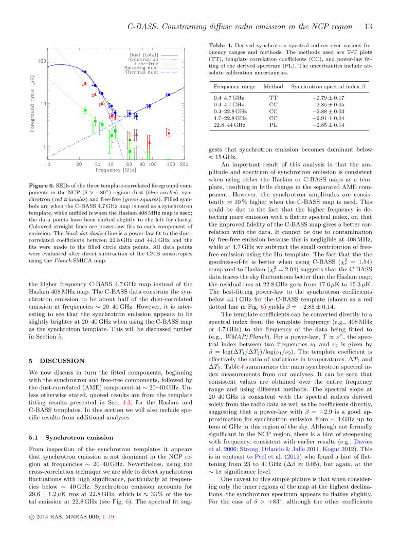
Figure 6. SEDs of the three template-correlated foreground com-ponents in the NCP (δ > +80◦) region: dust (blue circles), syn-

chrotron (red triangles) and free-free (green squares). Filled sym-

bols are when the C-BASS 4.7 GHz map is used as a synchrotrontemplate, while unfilled is when the Haslam 408 MHz map is used;

the data points have been shifted slightly to the left for clarity.Coloured straight lines are power-law fits to each component of

emission. The black dot-dashed line is a power-law fit to the dust-

correlated coefficients between 22.8 GHz and 44.1 GHz and thefits were made to the filled circle data points. All data points

were evaluated after direct subtraction of the CMB anisotropies

using the Planck SMICA map.

the higher frequency C-BASS 4.7 GHz map instead of theHaslam 408 MHz map. The C-BASS data constrain the syn-chrotron emission to be about half of the dust-correlatedemission at frequencies ∼ 20–40 GHz. However, it is inter-esting to see that the synchrotron emission appears to beslightly brighter at 20–40 GHz when using the C-BASS mapas the synchrotron template. This will be discussed furtherin Section 5.

5 DISCUSSION

We now discuss in turn the fitted components, beginningwith the synchrotron and free-free components, followed bythe dust-correlated (AME) component at ∼ 20–40 GHz. Un-less otherwise stated, quoted results are from the templatefitting results presented in Sect. 4.3, for the Haslam andC-BASS templates. In this section we will also include spe-cific results from additional analyses.

5.1 Synchrotron emission

From inspection of the synchrotron templates it appearsthat synchrotron emission is not dominant in the NCP re-gion at frequencies ∼ 20–40 GHz. Nevertheless, using thecross-correlation technique we are able to detect synchrotronfluctuations with high significance, particularly at frequen-cies below ∼ 40 GHz. Synchrotron emission accounts for29.6 ± 1.2µK rms at 22.8 GHz, which is ≈ 33 % of the to-tal emission at 22.8 GHz (see Fig. 6). The spectral fit sug-

Table 4. Derived synchrotron spectral indices over various fre-quency ranges and methods. The methods used are T-T plots

(TT), template correlation coefficients (CC), and power-law fit-

ting of the derived spectrum (PL). The uncertainties include ab-solute calibration uncertainties.

Frequency range Method Synchrotron spectral index β

0.4–4.7 GHz TT −2.79± 0.17

0.4–4.7 GHz CC −2.85± 0.050.4–22.8 GHz CC −2.88± 0.03

4.7–22.8 GHz CC −2.91± 0.04

22.8–44 GHz PL −2.85± 0.14

gests that synchrotron emission becomes dominant below≈ 15 GHz.

An important result of this analysis is that the am-plitude and spectrum of synchrotron emission is consistentwhen using either the Haslam or C-BASS maps as a tem-plate, resulting in little change in the separated AME com-ponent. However, the synchrotron amplitudes are consis-tently ≈ 10 % higher when the C-BASS map is used. Thiscould be due to the fact that the higher frequency is de-tecting more emission with a flatter spectral index, or, thatthe improved fidelity of the C-BASS map gives a better cor-relation with the data. It cannot be due to contaminationby free-free emission because this is negligible at 408 MHz,while at 4.7 GHz we subtract the small contribution of free-free emission using the Hα template. The fact that the thegoodness-of-fit is better when using C-BASS (χ2

r = 1.54)compared to Haslam (χ2

r = 2.04) suggests that the C-BASSdata traces the sky fluctuations better than the Haslam map;the residual rms at 22.8 GHz goes from 17.6µK to 15.3µK.The best-fitting power-law to the synchrotron coefficientsbelow 44.1 GHz for the C-BASS template (shown as a reddotted line in Fig. 6) yields β = −2.85± 0.14.

The template coefficients can be converted directly to aspectral index from the template frequency (e.g., 408 MHzor 4.7 GHz) to the frequency of the data being fitted to(e.g., WMAP/Planck). For a power-law, T ∝ νβ , the spec-tral index between two frequencies ν1 and ν2 is given byβ = log(∆T1/∆T2)/log(ν1/ν2). The template coefficient iseffectively the ratio of variations in temperatures, ∆T1 and∆T2. Table 4 summarizes the main synchrotron spectral in-dex measurements from our analyses. It can be seen thatconsistent values are obtained over the entire frequencyrange and using different methods. The spectral slope at20–40 GHz is consistent with the spectral indices derivedsolely from the radio data as well as the coefficients directly,suggesting that a power-law with β = −2.9 is a good ap-proximation for synchrotron emission from ∼ 1 GHz up totens of GHz in this region of the sky. Although not formallysignificant in the NCP region, there is a hint of steepeningwith frequency, consistent with earlier results (e.g., Davieset al. 2006; Strong, Orlando & Jaffe 2011; Kogut 2012). Thisis in contrast to Peel et al. (2012) who found a hint of flat-tening from 23 to 41 GHz (∆β ≈ 0.05), but again, at the∼ 1σ significance level.

One caveat to this simple picture is that when consider-ing only the inner regions of the map at the highest declina-tions, the synchrotron spectrum appears to flatten slightly.For the case of δ > +83◦, although the other coefficients

c© 2014 RAS, MNRAS 000, 1–19


are consistent to better than 2σ, the C-BASS synchrotroncoefficient at 22.8 GHz increases to 13.6±0.8µK mK−1, cor-responding to a synchrotron spectral index of β = −2.72 ±0.05. The other components do not change as significantlybecause the dust-correlated emission dominates the fluctua-tions at 23 GHz. This suggests that the synchrotron emissionin and around the two main AME dust clouds and NCP isslightly flatter than the large-scale emission from the Galac-tic plane. Nevertheless, the synchrotron emission remains asmall component relative to the total emission at 22.8 GHz.The equivalent spectral index from 0.4 GHz to 22.8 GHz re-mains consistent between the two sky areas, so if the flat-tening is real it is occurring above a frequency of a few GHzand then steepening again at higher frequencies (otherwisewe would see flatter indices above 4.7 GHz).

An important consideration for the interpretation ofsynchrotron emission is the presence of free-free emissionin the low-frequency radio data. At high Galactic latitudes,the Hα intensities are typically a few R at most. The Hαmap of the NCP region (Fig. 3) shows emission at a levelof ∼ 1 R with a peak of 3.7 R on a background of ≈ 0.5–1 R; see Section 5.2. A typical high-latitude Hα intensityof 1 R corresponds to 51 mK at 408 MHz and 0.3 mK at4.7 GHz (Dickinson, Davies & Davis 2003). Therefore thecontribution from free-free at high latitudes is negligible at408 MHz (typical fluctuations of ∼ 10 K) and a small con-tribution at 4.7 GHz (typical fluctuations ≈ 5 mK). Eventhough it had little impact on the quoted results, we sub-tracted the free-free contribution at 4.7 GHz using the Hαmap and a conversion factor of 0.32 mK R−1. As a furthertest, we performed template-fitting of the C-BASS map it-self, using the 408 MHz and Hα maps as tracers of the syn-chrotron and free-free emission, respectively. We do not de-tect Hα-correlated emission in the NCP region at 4.7 GHz,with a template coefficient of 0.29 ± 0.31 mK R−1, which isconsistent with theoretical expectations. Virtually all of thesignal at 4.7 GHz can be accounted for by the 408 MHz tem-plate, with a coefficient of 935± 72 mK K−1, correspondingto β = −2.85 ± 0.05. This can be contrasted with emissionfrom the Galactic disk, which emits a much larger fractionof free-free emission at 4.7 GHz (Irfan et al. 2015).

Table 5 lists the rms values for each component fromthe cross-correlation analysis for δ > +80◦, calculated bymultiplying the cross-correlation template coefficients by therms fluctuations in the template map for this region. Tak-ing into account correlations between the templates givesa total rms of 89.4 ± 4.1µK at 22.8 GHz. We also list therms values from the corresponding Planck 2015 Comman-der component separation products (Planck Collaborationet al. 2016a), scaled to 22.8 GHz. We can see that in thecross-correlation analysis using C-BASS, although the AMEdominates the fluctuations, the synchrotron emission con-tributes almost three times more rms fluctuations comparedto the Planck Commander solution. This is due to thefact that the Planck Commander analysis used only onelow-frequency data point at 408 MHz, which meant thatthe synchrotron spectrum had to be effectively fixed. Theirmodel had an effective spectral index of β ≈ −3.05 ± 0.05above 1 GHz (Planck Collaboration et al. 2016c), while theC-BASS data prefers a slightly flatter index of β ≈ −2.9.

Finally, we comment on the apparent upturn in the syn-chrotron spectrum above ∼ 90 GHz (Fig. 6). At these fre-

Table 5. RMS fluctuations at 22.8 GHz of each component for

δ > +80◦ from the cross-correlation (CC) analysis and from

the Planck 2015 Commander component separation products(Planck Collaboration et al. 2016a). Units are µK.

Component CC Planck 2015

Synchrotron 29.6± 1.2 11.8Free-free 7.0± 1.0 46.9

AME / dust 55.0± 2.0 45.4

Thermal dust . . . 1.2Total foreground 88.8± 3.6 84.0

quencies the synchrotron component accounts for � 10%of the total emission and therefore is difficult to separatefrom the much brighter dust emission and is also partially(spatially) correlated. This is partially reflected in the largererror bars and therefore we do not believe the upturn to bea real effect.

5.2 Free-free emission

The Hα-correlated component is expected to be due to free-free emission (Dickinson, Davies & Davis 2003). For an elec-tron temperature Te = 8000 K, typical of the diffuse ISM,we would expect to see Hα template coefficients of 11.4,7.8, 5.23, 3.28 and 1.11µK R−1, for frequencies of 22.8, 28.4,33.0, 40.7, 44.1 GHz, respectively. It also assumes that thecorrection for dust extinction along the line of sight has beendone accurately, which renders the standard Hα templatesuseless at very low Galactic latitudes (Dickinson, Davies &Davis 2003). The theoretical values also assume local ther-modynamic equilibrium, 8 per cent contribution from he-lium, and that there is no scattering of Hα from elsewhereoff dust grains. The amount of scattered Hα light is notclear, with earlier predictions in the range 5–20 % (Wood& Reynolds 1999), while more recent work has suggest thatit could be more significant along some lines of sight (Seon& Witt 2012; Brandt & Draine 2012) and possibly up to50% or more (Witt et al. 2010). This would in turn reducethese coefficients by up to a half, giving better agreementwith theory (Banday et al. 2003; Davies et al. 2006; Dobler,Draine & Finkbeiner 2009; Ghosh et al. 2012).

From our analysis, the free-free emission is very weakin the NCP region. The free-free brightness has an rms of7.0± 1.0µK at 22.8 GHz (Table 5), corresponding to ≈ 6%of the total emission. Nevertheless, the Hα-correlated val-ues in Table 3 are consistent with theoretical expectations;at 22.8 GHz we expect ≈ 11µK R−1 for typical electrontemperatures (Dickinson, Davies & Davis 2003). Moreover,while the uncertainties are relatively large, the independentcoefficients plotted in Fig. 6 precisely follow the spectral de-pendence expected for free-free emission (β ≈ −2.1) upto 44 GHz and higher. This is good reassurance that thetemplate fits are yielding physically meaningful results. Aprevious analysis of the Hα fluctuations in the NCP region(δ > +81◦) by Gaustad, McCullough & van Buren (1996)found an upper limit of 0.5 R on 1◦ scales, corresponding to< 6µK at 22.8 GHz. This is consistent with our analysis atthe 1σ level. We note that the Planck 2015 free-free mapgives a much larger rms amplitude of 46.9µK (Table 5), atthe expense of both the AME and synchrotron components.

c© 2014 RAS, MNRAS 000, 1–19


This is the largest discrepancy between the two analyses. Asdiscussed and demonstrated by Planck Collaboration et al.(2016c), the Commander free-free solution appears to beover-estimated (typically by a factor of several) due to alias-ing of the low frequency (synchrotron or free-free or AME)components by the spectrum alone.

The Hα coefficients from our analysis are consistentwith expectations from theory, for electron temperatures inthe range Te ≈ 7000–10000 K; this indicates that scatteredHα is not a major issue in this region of sky. They are alsoconsistent when using either of the synchrotron templates.Note that we chose to subtract the free-free component fromthe C-BASS 4.7 GHz map to ensure it was dominated bysynchrotron emission. When using the raw 4.7 GHz withouta free-free correction, we naturally found a lower value forthe template coefficient of 9.9± 1.9µK R−1 at 22.8 GHz, in-dicating that residual free-free emission in the 4.7 GHz mapis having a small impact, at least on the free-free solution.Fortunately, it has negligible impact on the other templateresults, with the values changing by less than 0.2σ for boththe synchrotron- and dust-correlated coefficients. This high-lights that the free-free emission is relatively weak at allmicrowave frequencies.

The two Hα templates (F03 and D03) also give slightlydifferent results (but consistent within the uncertainties),which can be attributed largely to stellar residuals in the Hαmaps that have been treated differently. The Hα-correlatedtemplate coefficient at 22.8 GHz when using F03 was 18.2±2.9µK R−1, slightly higher than for D03, which is expecteddue to the small fluctuations in the F03 version of the map.This also had a minor impact on the synchrotron and dustcoefficients but is consistent to within 1.5σ. The dust red-dening E(B−V ) map of Schlegel, Finkbeiner & Davis (1998)can be used to estimate the maximum level of dust extinc-tion assuming all the dust is in front of the ionized gas (Dick-inson, Davies & Davis 2003). At the original 6.1 arcmin res-olution, the main dust feature in this region has extinctionvalues in the range ≈ 0.2–0.7 mag; at 1◦ resolution the twodust emission peaks are at a value of ≈ 0.45 mag, corre-sponding to a maximum dust absorbing factor of ≈ 1.5. It istherefore possible that the Hα intensity is under-estimatedin this region by ≈ 20–30 % (about half of the maximumvalue). This would not have a significant effect on the syn-chrotron and AME results because the free-free componentis sub-dominant, being ≈ 7 % of the total emission.

In summary, the D03 Hα template appears to trace free-free emission more reliably than the F03 map, with an am-plitude that is as expected for typical electron temperaturesof Te ≈ 7000–10000 K. The free-free emission at AME fre-quencies (≈ 20–40 GHz) in the NCP region appears to be asmall portion of the total emission, and therefore assump-tions about the template and dust extinction have little ef-fect on the AME amplitude.

5.3 AME

Our results show a significant detection of dust-correlatedemission, particularly in the ∼20–40 GHz range. The dust-correlated emission (AME) is much brighter than can beaccounted for by thermal dust (which would have a fallingspectrum with decreasing frequency) and synchrotron/free-free emission as traced by the foreground templates. The

Table 6. AME cross-correlation template coefficients at 22.8 GHzand χ2

r values for different dust templates, ordered in terms of

decreasing goodness-of-fit.

Template Correlation Coeff. Unit χ2r

τ353 9.52± 0.34 K 1.54

Planck 545 GHz 67± 2 µK (MJy sr−1)−1 1.60

FDS94 5.16± 0.19 mK mK−1 1.62Planck 857 GHz 22.4± 0.8 µK (MJy sr−1)−1 1.63

Planck 353 GHz 875± 32 µK mK−1 1.63

Dust radiance < 563± 20 K (W m−2 sr−1)−1 2.12IRIS 100µm 31.0± 1.1 µK (MJy sr−1)−1 2.90

rms of the dust-correlated component at 22.8 GHz is 55.0±2.0µK at 22.8 GHz, which accounts for ≈ 60% of the totalrms (Table 5).

The main result of this paper is the lack of change in theAME signal relative to the FIR data, when using the higherfrequency C-BASS 4.7 GHz template compared to the tra-ditional Haslam 408 MHz map. This is a similar result tothose previously found when using a 2.3 GHz map as a syn-chrotron template (Peel et al. 2012), who found the AMEamplitude changed by only 7%. For our baseline fit, whenusing the τ353 map as the dust template, we find coefficientsat 22.8 GHz of 9.93± 0.35 K and 9.52± 0.34 K per unit τ353(Table 3), when using the Haslam and C-BASS maps as syn-chrotron templates, respectively, i.e. they are consistent atthe ≈ 1σ level with just a 4% change in amplitude.

Our main result is consistent with the spectral indicesfor synchrotron emission that are almost constant across theentire radio/microwave band (see Sect. 5.1). An additionalflatter (harder) spectrum component of synchrotron is notdetected at 4.7 GHz. For synchrotron emission to explainthe bulk of the AME, it would have to have a much flatterspectrum; a value of β ≈ −2.3 would be needed to extrapo-late the ∼ 3 mK rms fluctuations at 4.7 GHz to the ∼ 80µKfluctuations observed at 22.8 GHz (after removing the CMBand free-free contribution). However, in practice it wouldneed to be even flatter than this, since the observed emis-sion at 4.7 GHz does not correlate well with the AME, andhence a flat synchrotron AME component would need to besubdominant at 4.7 GHz.

We find similar levels of AME in the NCP region, rela-tive to the standard dust templates, to those measured pre-viously. Table 6 lists the AME cross-correlation template co-efficients at 22.8 GHz and χ2

r values for each dust template.We adopt τ353 as our default template since it formally pro-vided the best fit to the microwave data, with map residu-als of 15µK rms. Our best value of 9.52± 0.34 K compareswell with the high-latitude (|b| > 10◦) value of 9.7 ± 1.0 K(Planck Collaboration et al. 2016c). Hensley, Draine & Meis-ner (2016) found a value of 7.9 ± 2.6 K at 30 GHz, whichis also consistent. We find slightly larger fluctuations inthe AME at 22.8 GHz (55 ± 2µK) compared to the Planckproducts (45.4µK), but they are comparable (Table 5). Thisshows that even with very different component separationtechniques, the AME is a strong component of the emissionat frequencies ≈ 20–40 GHz.

We tried several other standard dust templates, listedin Tables 2 and 6. The worst template is the 100µm tem-plate, which is confirmed by the Pearson correlation coeffi-

c© 2014 RAS, MNRAS 000, 1–19


cients at 22.8 GHz (where AME is dominant), as shown inSect. 3.3. It is also evident in the residual maps at 22.8 GHzpresented in Fig. 5; the residual map rms at 22.8 GHz in-creases from 15µK to 21µK rms. This is presumably dueto variations in the dust composition or temperature, whichsignificantly modulates the response at wavelengths near thepeak of the spectrum at ∼ 100µm but has negligible effectat longer wavelengths (e.g., Finkbeiner 2004; Tibbs, Pal-adini & Dickinson 2012). Nevertheless, we measured cou-pling coefficients of 31.0± 1.1µK (MJy sr−1)−1 at 22.8 GHzand 9.9 ± 0.7µK (MJy sr−1)−1 at 33.0 GHz. This compareswell with the ≈ 10µK (MJy sr−1)−1 at 33.0 GHz that hasbeen observed before (Banday et al. 2003; de Oliveira-Costaet al. 2004; Davies et al. 2006). This can also be comparedwith the dust-correlation measured originally by Leitch et al.(1997), which when extrapolated to 22.8 GHz, correspondsto 77µK (MJy sr−1)−1. This value is higher because it is adirect (single template) correlation, therefore neglecting anydust-correlated synchrotron/free-free emission. Also, theirbest-fitting spectral index of −2.2 is flatter than most mea-surements since then, which increases the relative amplitudeat higher frequencies. The interpretation is that about halfof the total dust-correlated signal at 20–40 GHz is due toAME.

Interestingly, unlike the results of Hensley, Draine &Meisner (2016) the map of dust radiance (<) was foundnot to trace AME as well as τ353 or any of the PlanckHFI maps. Nevertheless, we found similar amplitudes tothose estimated at high latitudes. For example, for thecase of the dust radiance template, we found a coeffi-cient of 563 ± 20 K (W m−2 sr−1)−1 compared to 226 ±44 K (W m−2 sr−1)−1 at 30 GHz. Surprisingly, the mucholder FDS94 model (Finkbeiner, Davis & Schlegel 1999)provided almost as good a fit as τ353. Our coefficient of5.16±0.19 mK mK−1 is slightly lower than the equivalent re-gion 6 of Davies et al. (2006) who found 6.7±0.7 mK mK−1.When adopting the Haslam synchrotron template we ob-tained a consistent value of 5.38±0.19 mK mK−1. The slightdifference is mostly due to the slightly different sky areas andmasking used.

From Fig. 6 it is clear that using the much higherfrequency synchrotron template from C-BASS makes lit-tle difference to the dust-correlated (AME) component, atleast in this region of the sky. This indicates that thereis no strong component of flat-spectrum synchrotron emis-sion. The spectrum of the dust-correlated component alsoappears to be well approximated at ∼ 20–40 GHz by apower-law with a best-fitting slope of β = −3.23 ± 0.13,which is slightly steeper but remarkably close to the spec-trum of the synchrotron component (β ≈ −2.9). We fit-ted a spinning dust model, using the spdust2 code (Ali-Haımoud, Hirata & Dickinson 2009; Silsbee, Ali-Haımoud &Hirata 2011), adopting the parameters for the Cold NeutralMedium (CNM) as suggested by Draine & Lazarian (1998a).This gave a poor fit because this particular model spectrumpeaks at 33 GHz (in flux density units). We therefore in-cluded a frequency shift (in log-space) of the CNM spinningdust spectrum, which provided a good fit with a peak fre-quency of 23 GHz, as shown in Fig. 6. However, there is anindication that there is excess emission in the range ≈ 50–100 GHz. This is likely a failure of the simple single compo-nent CNM spinning dust model.

In reality, there will be a range of dust parti-cles/environments along the line-of-sight that will tendto broaden the spectrum, and which motivated the two-component model by Planck Collaboration et al. (2016a,c).Note that spinning dust models generally predict broadlypeaked emission spectra with a FWHM in frequency approx-imately twice the peak frequency; for example, the WNMmodel of Draine & Lazarian (1998b) has a peak at 22 GHzin flux density, with half-max points at 13 GHz and 37 GHz.The location of the peak is determined by a combinationof the nanoparticle size distribution, the electric dipole mo-ment, and the excitation conditions.

Using a single component model results in a thermaldust emissivity index of β = +1.25 ± 0.13, which is signifi-cantly flatter than has been measured for the majority of thesky with β ≈ 1.6 (e.g., Planck Collaboration et al. 2014a).The low value is within the range measured by Planck butis sensitive to which CMB map is used and over which fre-quencies are being fitted. It does not change the results forAME, which dominates at lower frequencies where the ther-mal dust has a minimal contribution. Given the lack of al-ternatives, the spinning dust mechanism appears to be themost viable explanation for the diffuse AME observed in theNCP region.

6 CONCLUSIONS

We have re-analysed the NCP region (δ > +80◦) inWMAP/Planck data to study the diffuse foregrounds. Weused template maps of synchrotron (low-frequency radiomaps), free-free (Hα maps) and dust emission (sub-mm/FIRmaps) to fit to WMAP/Planck data at 22.8 GHz and above.In addition to the standard Haslam 408 MHz map, weused new C-BASS data at 4.7 GHz as a tracer of syn-chrotron emission. C-BASS data are of higher quality thanthe Haslam et al. (1982) data, which are known to containsignificant striations and other calibration issues. More im-portantly, at a frequency of ≈ 4.7 GHz, C-BASS data aremuch closer to the frequencies observed by WMAP/Planckand therefore should be more representative of foregroundsat microwave frequencies. In particular, if there is a signif-icant hard (flat spectrum) component of synchrotron radi-ation, then the C-BASS maps should be a more reliablesynchrotron template.

We have found that the dust-correlated AME compo-nent accounts for the bulk (≈ 60%) of the foreground rmsin the NCP region and that it does not change significantlywhen including the C-BASS 4.7 GHz map. The synchrotronemission has a spectrum close to β = −2.90 ± 0.05 whenconsidering the low frequency data alone via T-T plots, thecross-correlation coefficients directly, or when fitting to theSED of coefficients in the range 20–40 GHz. This indicatesthat a power-law is a good model for the synchrotron emis-sion from a frequency of 0.4 GHz up to tens of GHz andthat there is no strong component of flat-spectrum (harder)synchrotron emission, at least in the NCP region. The syn-chrotron component accounts for approximately half the rmsbrightness at 22.8 GHz. We find that the D03 version of theHα map correlates better with microwave data than the F03map, due to low level residual artifacts in the maps. Fortu-

c© 2014 RAS, MNRAS 000, 1–19


nately, free-free emission is relatively weak at high latitudesand accounts for ≈ 6 % of the total signal at 22.8 GHz.

We preferred the thermal dust optical depth at 353 GHzas our tracer of AME since it gave the best overall fit. Wefound a best-fitting template coefficient of 9.52± 0.34 K perunit τ353 at 22.8 GHz, which agrees well with previous mea-surements on different regions of the sky. Other templates,such as dust radiance and FDS94 gave similar results butwith slightly larger residuals. The most discrepant of thedust tracers was the IRIS 100µm map, due to variations indust temperature within the region, which modulates thespatial morphology at wavelengths near 100µm

A power-law provides a good fit to the AME spectrumabove 20 GHz. Alternatively, it can be well-fitted by a shiftedspinning dust model, with a peak frequency (flux densityunits) around 23 GHz. However, in this case the thermaldust emissivity index flattens to ≈ +1.3. This is likely afailure of a simple single component spinning dust model,which is inevitably narrower than the true distribution ofdust particles and environments.

The observations for the northern C-BASS survey arenow complete and the southern survey is just beginning.With full-sky C-BASS maps we will be able to investigatethe AME across the whole sky and to investigate the possi-ble contribution of a harder spectrum of synchrotron radia-tion. Future papers will include applying T-T plot (Jew etal., in prep.) and template fitting (Harper et al., in prep.)techniques to the high latitude sky. We will also use more ad-vanced component separation techniques such as parametricfitting (e.g., Eriksen et al. 2008). With the wealth of highprecision data covering a wide range of frequencies, includ-ing new data from S-PASS (Krachmalnicoff et al. 2018) andQUIJOTE (Genova-Santos et al. 2015), we should be ableto fit for all these components as a function of position onthe sky.

ACKNOWLEDGMENTS

The C-BASS project is a collaboration between Oxfordand Manchester Universities in the UK, the California In-stitute of Technology in the U.S.A., Rhodes University,UKZN and the South African Radio Observatory in SouthAfrica, and the King Abdulaziz City for Science and Tech-nology (KACST) in Saudi Arabia. It has been supported bythe NSF awards AST-0607857, AST-1010024, AST-1212217,and AST-1616227, and NASA award NNX15AF06G, theUniversity of Oxford, the Royal Society, STFC, and theother participating institutions. This research was also sup-ported by the South African Radio Astronomy Observa-tory, which is a facility of the National Research Founda-tion, an agency of the Department of Science and Tech-nology. We would like to thank Russ Keeney for techni-cal help at OVRO. CD acknowledges support from an ERCStarting (Consolidator) Grant (no. 307209). CD also thanksthe California Institute of Technology for their hospitalityand hosting during several extended visits. MWP acknowl-edges funding from a FAPESP Young Investigator fellow-ship, grant 2015/19936-1. We make use of the HEALPixpackage (Gorski et al. 2005), IDL astronomy library andPython astropy, matplotlib, numpy, healpy, and scipy pack-ages. This research has made use of the NASA/IPAC Ex-

tragalactic Database (NED) which is operated by the JetPropulsion Laboratory, California Institute of Technology,under contract with the National Aeronautics and SpaceAdministration. The C-BASS collaboration would like to re-member the late Prof. Rodney D. Davies and Prof. RichardJ. Davis, who were both strong supporters of the C-BASSproject (http://cbass.web.ox.ac.uk).

REFERENCES

Ali-Haımoud Y., Hirata C. M., Dickinson C., 2009, MN-RAS, 395, 1055

Alves M. I. R., Davies R. D., Dickinson C., Calabretta M.,Davis R., Staveley-Smith L., 2012, MNRAS, 422, 2429

AMI Consortium et al., 2011, MNRAS, 415, 2708Armitage-Caplan C., Dunkley J., Eriksen H. K., DickinsonC., 2012, MNRAS, 424, 1914

Banday A. J., Dickinson C., Davies R. D., Davis R. J.,Gorski K. M., 2003, MNRAS, 345, 897

Bennett C. L. et al., 2003, ApJS, 148, 97Bennett C. L. et al., 2013, ApJS, 208, 20Brandt T. D., Draine B. T., 2012, ApJ, 744, 129Casassus S., Cabrera G. F., Forster F., Pearson T. J., Read-head A. C. S., Dickinson C., 2006, ApJ, 639, 951

Casassus S. et al., 2008, MNRAS, 391, 1075Condon J. J., Cotton W. D., Greisen E. W., Yin Q. F.,Perley R. A., Taylor G. B., Broderick J. J., 1998, AJ, 115,1693

Davies R. D., Dickinson C., Banday A. J., Jaffe T. R.,Gorski K. M., Davis R. J., 2006, MNRAS, 370, 1125

Davies R. D., Watson R. A., Gutierrez C. M., 1996, MN-RAS, 278, 925

de Oliveira-Costa A., Tegmark M., Davies R. D., GutierrezC. M., Lasenby A. N., Rebolo R., Watson R. A., 2004,ApJ, 606, L89

de Zotti G., Massardi M., Negrello M., Wall J., 2010,A&A Rev., 18, 1

Delabrouille J., Cardoso J., 2009, in Lecture Notes inPhysics, Berlin Springer Verlag, Vol. 665, Data Analy-sis in Cosmology, V. J. Martınez, E. Saar, E. Martınez-Gonzalez, & M.-J. Pons-Borderıa, ed., pp. 159–205

Dickinson C. et al., 2018, New Astronomy Reviews, 80, 1Dickinson C. et al., 2010, MNRAS, 407, 2223Dickinson C. et al., 2009, ApJ, 690, 1585Dickinson C., Davies R. D., Davis R. J., 2003, MNRAS,341, 369

Dickinson C., Peel M., Vidal M., 2011, MNRAS, 418, L35Dobler G., Draine B., Finkbeiner D. P., 2009, ApJ, 699,1374

Draine B. T., Hensley B., 2013, ApJ, 765, 159Draine B. T., Lazarian A., 1998a, ApJ, 494, L19Draine B. T., Lazarian A., 1998b, ApJ, 508, 157Draine B. T., Lazarian A., 1999, ApJ, 512, 740Dunkley J. et al., 2009a, in American Institute of PhysicsConference Series, Vol. 1141, American Institute ofPhysics Conference Series, Dodelson S., Baumann D.,Cooray A., Dunkley J., Fraisse A., Jackson M. G., KogutA., Krauss L., Zaldarriaga M., Smith K., eds., pp. 222–264

Dunkley J. et al., 2009b, ApJ, 701, 1804Erickson W. C., 1957, ApJ, 126, 480

c© 2014 RAS, MNRAS 000, 1–19

http://cbass.web.ox.ac.uk


Eriksen H. K., Jewell J. B., Dickinson C., Banday A. J.,Gorski K. M., Lawrence C. R., 2008, ApJ, 676, 10

Errard J., Stompor R., 2012, Phys.Rev.D, 85, 083006Finkbeiner D. P., 2003, ApJS, 146, 407Finkbeiner D. P., 2004, ApJ, 614, 186Finkbeiner D. P., Davis M., Schlegel D. J., 1999, ApJ, 524,867

Finkbeiner D. P., Schlegel D. J., Frank C., Heiles C., 2002,ApJ, 566, 898

Gaustad J. E., McCullough P. R., van Buren D., 1996,PASP, 108, 351

Genova-Santos R. et al., 2017, MNRAS, 464, 4107Genova-Santos R. et al., 2015, in Highlights of Spanish As-trophysics VIII, Cenarro A. J., Figueras F., Hernandez-Monteagudo C., Trujillo Bueno J., Valdivielso L., eds., pp.207–212 [arXiv:1504.03514]

Ghosh T., Banday A. J., Jaffe T., Dickinson C., Davies R.,Davis R., Gorski K., 2012, MNRAS, 422, 3617

Gold B. et al., 2011, ApJS, 192, 15Gorski K. M., Hivon E., Banday A. J., Wandelt B. D.,Hansen F. K., Reinecke M., Bartelmann M., 2005, ApJ,622, 759

Gregory P. C., Scott W. K., Douglas K., Condon J. J.,1996, ApJS, 103, 427

Haffner L. M., Reynolds R. J., Tufte S. L., Madsen G. J.,Jaehnig K. P., Percival J. W., 2003, ApJS, 149, 405

Hargrave P. J., McEllin M., 1975, MNRAS, 173, 37Haslam C. G. T., Salter C. J., Stoffel H., Wilson W. E.,1982, A&AS, 47, 1

Healey S. E., Fuhrmann L., Taylor G. B., Romani R. W.,Readhead A. C. S., 2009, AJ, 138, 1032

Hensley B. S., Draine B. T., Meisner A. M., 2016, ApJ,827, 45

Hoang T., Lazarian A., 2016, ApJ, 821, 91Holler C. M. et al., 2013, IEEE Transactions on Antennasand Propagation, 61, 117

Irfan M. O., 2014, PhD thesis, The University of Manch-ester, Oxford Road, Manchester, M13 9PL, U.K.

Irfan M. O. et al., 2015, MNRAS, 448, 3572Jaffe T. R., Banday A. J., Leahy J. P., Leach S., StrongA. W., 2011, MNRAS, 416, 1152

Jonas J. L., Baart E. E., Nicolson G. D., 1998, MNRAS,297, 977

Jones M. E. et al., 2018, MNRAS, 480, 3224King O. G. et al., 2010, in Society of Photo-Optical In-strumentation Engineers (SPIE) Conference Series, Vol.7741, Society of Photo-Optical Instrumentation Engineers(SPIE) Conference Series

King O. G. et al., 2014, MNRAS, 438, 2426Kogut A., 2012, ApJ, 753, 110Kogut A., Banday A. J., Bennett C. L., Gorski K. M.,Hinshaw G., Smoot G. F., Wright E. I., 1996, ApJ, 464,L5

Kogut A. et al., 2007, ApJ, 665, 355Kogut A. et al., 2011, ApJ, 734, 4Krachmalnicoff N. et al., 2018, A&A, 618, A166Kuhr H., Pauliny-Toth I. I. K., Witzel A., Schmidt J.,1981a, AJ, 86, 854

Kuhr H., Witzel A., Pauliny-Toth I. I. K., Nauber U.,1981b, A&AS, 45, 367

Lagache G., 2003, A&A, 405, 813Lawson K. D., Mayer C. J., Osborne J. L., Parkinson M. L.,

1987, MNRAS, 225, 307Leach S. M. et al., 2008, A&A, 491, 597Leitch E. M., Readhead A. C. S., Pearson T. J., MyersS. T., 1997, ApJ, 486, L23

Liu J., Cui L., Liu X., Ding Z., Song H.-G., 2014, Journalof Astrophysics and Astronomy

Lopez-Caraballo C. H., Rubino-Martın J. A., Rebolo R.,Genova-Santos R., 2011, ApJ, 729, 25

Macellari N., Pierpaoli E., Dickinson C., Vaillancourt J. E.,2011, MNRAS, 418, 888

Markwardt C. B., 2009, in Astronomical Society of the Pa-cific Conference Series, Vol. 411, Astronomical Data Anal-ysis Software and Systems XVIII, Bohlender D. A., Du-rand D., Dowler P., eds., p. 251

Mingaliev M. G., Sotnikova Y. V., Bursov N. N., KardashevN. S., Larionov M. G., 2007, Astronomy Reports, 51, 343

Miville-Deschenes M., Lagache G., 2005, ApJS, 157, 302Onic D., 2013, Ap&SS, 346, 3Orlando E., Strong A., 2013, MNRAS, 436, 2127Peel M. W., Dickinson C., Davies R. D., Banday A. J.,Jaffe T. R., Jonas J. L., 2012, MNRAS, 424, 2676

Planck Collaboration et al., 2014a, A&A, 571, A11Planck Collaboration et al., 2011a, A&A, 536, A21Planck Collaboration et al., 2016a, A&A, 594, A10Planck Collaboration et al., 2016b, A&A, 594, A9Planck Collaboration et al., 2014b, A&A, 571, A13Planck Collaboration et al., 2013a, A&A, 557, A53Planck Collaboration et al., 2016c, A&A, 594, A25Planck Collaboration et al., 2014c, A&A, 565, A103Planck Collaboration et al., 2016d, A&A, 594, A26Planck Collaboration et al., 2013b, A&A, 554, A139Planck Collaboration et al., 2011b, A&A, 536, A20Planck Collaboration et al., 2016e, A&A, 596, A109Planck Collaboration et al., 2018a, submitted to A&A[arXiv:1807.06205]

Planck Collaboration et al., 2018b, submitted to A&A[arXiv:1807.06208]

Platania P., Bensadoun M., Bersanelli M., de Amici G.,Kogut A., Levin S., Maino D., Smoot G. F., 1998, ApJ,505, 473

Reich P., Reich W., 1986, A&AS, 63, 205Reich P., Reich W., 1988, A&AS, 74, 7Reich P., Testori J. C., Reich W., 2001, A&A, 376, 861Reich W., 1982, A&AS, 48, 219Remazeilles M., Dickinson C., Banday A. J., Bigot-SazyM.-A., Ghosh T., 2015, MNRAS, 451, 4311

Remazeilles M., Dickinson C., Eriksen H. K. K., WehusI. K., 2016, MNRAS, 458, 2032

Ricci R. et al., 2013, MNRAS, 435, 2793Righini S. et al., 2012, MNRAS, 426, 2107Rubino-Martın J. A., Lopez-Caraballo C. H., Genova-Santos R., Rebolo R., 2012, Advances in Astronomy, 2012

Scaife A. M. M. et al., 2009, MNRAS, 400, 1394Schlegel D. J., Finkbeiner D. P., Davis M., 1998, ApJ, 500,525

Seon K.-I., Witt A. N., 2012, ApJ, 758, 109Silsbee K., Ali-Haımoud Y., Hirata C. M., 2011, MNRAS,411, 2750

Strong A. W., Orlando E., Jaffe T. R., 2011, A&A, 534,A54

Sutton D. et al., 2010, MNRAS, 407, 1387Tibbs C. T. et al., 2011, MNRAS, 418, 1889

c© 2014 RAS, MNRAS 000, 1–19


Tibbs C. T., Paladini R., Dickinson C., 2012, Advances inAstronomy, 2012, 124931

Tibbs C. T., Scaife A. M. M., Dickinson C., Paladini R.,Davies R. D., Davis R. J., Grainge K. J. B., Watson R. A.,2013, ApJ, 768, 98

Turtle A. J., Pugh J. F., Kenderdine S., Pauliny-TothI. I. K., 1962, MNRAS, 124, 297

Watson R. A., Rebolo R., Rubino-Martın J. A., Hilde-brandt S., Gutierrez C. M., Fernandez-Cerezo S., Hoyland

R. J., Battistelli E. S., 2005, ApJ, 624, L89Weiland J. L. et al., 2011, ApJS, 192, 19Williams M. J., Bureau M., Cappellari M., 2010, MNRAS,409, 1330

Winkel B., Kerp J., Floer L., Kalberla P. M. W., BenBekhti N., Keller R., Lenz D., 2016, A&A, 585, A41

Witt A. N., Gold B., Barnes, III F. S., DeRoo C. T., VijhU. P., Madsen G. J., 2010, ApJ, 724, 1551

Wood K., Reynolds R. J., 1999, ApJ, 525, 799

c© 2014 RAS, MNRAS 000, 1–19

the c-band all-sky survey (c-bass): constraining di use ... · valley radio observatory,...

Documents