the caloron correspondence and odd di erential k-theory

The Caloron Correspondence and

Odd Differential K-theory

Vincent S. Schlegel

Thesis submitted in partial fulfilmentof the requirements for the degree of

Master of Philosophy

in

Pure Mathematics

at The University of Adelaide

School of Mathematical Sciences

July 2013

arX

iv:1

309.

2601

v1 [

mat

h.D

G]

10

Sep

2013

Contents

Abstract i

Signed statement iii

Acknowledgements vii

Introduction 1

1 The caloron correspondence 7

1.1 The caloron correspondence . . . . . . . . . . . . . . . . . . . . . . . . . . . 7

1.1.1 The caloron correspondence . . . . . . . . . . . . . . . . . . . . . . . 8

1.1.2 Higgs fields and connections . . . . . . . . . . . . . . . . . . . . . . . 11

1.1.3 String classes . . . . . . . . . . . . . . . . . . . . . . . . . . . . . . . 15

1.2 The based case . . . . . . . . . . . . . . . . . . . . . . . . . . . . . . . . . . 18

1.2.1 The path fibration and string classes . . . . . . . . . . . . . . . . . . 21

2 The string potentials 29

2.1 Construction of the string potentials . . . . . . . . . . . . . . . . . . . . . . 29

2.1.1 The relative string potentials . . . . . . . . . . . . . . . . . . . . . . 32

2.1.2 The total string potentials . . . . . . . . . . . . . . . . . . . . . . . . 34

2.2 String potentials and secondary characteristic classes . . . . . . . . . . . . . 37

3 Ω vector bundles 43

3.1 Preliminaries . . . . . . . . . . . . . . . . . . . . . . . . . . . . . . . . . . . 43

3.1.1 The caloron correspondence for vector bundles . . . . . . . . . . . . 48

3.1.2 Operations on ΩVect . . . . . . . . . . . . . . . . . . . . . . . . . . . 50

3.1.3 Ω vector bundles and LC∞(M)-modules . . . . . . . . . . . . . . . . 54

3.2 Higgs fields and module connections . . . . . . . . . . . . . . . . . . . . . . 58

3.2.1 The geometric caloron correspondence . . . . . . . . . . . . . . . . . 64

3.3 Hermitian structures . . . . . . . . . . . . . . . . . . . . . . . . . . . . . . . 69

3.3.1 Hermitian Higgs fields and module connections . . . . . . . . . . . . 71

3.4 Applications to K-theory . . . . . . . . . . . . . . . . . . . . . . . . . . . . 74

3.4.1 Topological K-theory . . . . . . . . . . . . . . . . . . . . . . . . . . 74

3.4.2 The functor K−1 . . . . . . . . . . . . . . . . . . . . . . . . . . . . . 77

3.4.3 The total string form and the Chern character . . . . . . . . . . . . 81

4 The Ω model for odd differential K-theory 87

4.1 Structured vector bundles . . . . . . . . . . . . . . . . . . . . . . . . . . . . 88

4.1.1 The Simons-Sullivan model . . . . . . . . . . . . . . . . . . . . . . . 88

4.1.2 Structured Ω vector bundles . . . . . . . . . . . . . . . . . . . . . . . 924.2 The Ω model . . . . . . . . . . . . . . . . . . . . . . . . . . . . . . . . . . . 99

4.2.1 The TWZ extension and the action of forms on K−1 . . . . . . . . . 1004.2.2 Odd differential K-theory . . . . . . . . . . . . . . . . . . . . . . . . 105

Conclusions and further work 111

A Infinite-dimensional manifolds 113A.1 Frechet spaces and Frechet manifolds . . . . . . . . . . . . . . . . . . . . . . 113A.2 Mapping manifolds . . . . . . . . . . . . . . . . . . . . . . . . . . . . . . . . 115A.3 The path fibration . . . . . . . . . . . . . . . . . . . . . . . . . . . . . . . . 116A.4 Direct limit manifolds . . . . . . . . . . . . . . . . . . . . . . . . . . . . . . 117

B Integration over the fibre 121B.1 For differential forms . . . . . . . . . . . . . . . . . . . . . . . . . . . . . . . 121B.2 For singular cohomology . . . . . . . . . . . . . . . . . . . . . . . . . . . . . 124

C Differential extensions 129C.1 Axioms for differential extensions . . . . . . . . . . . . . . . . . . . . . . . . 129C.2 Uniqueness of differential extensions . . . . . . . . . . . . . . . . . . . . . . 131

Bibliography 132

Abstract

The caloron correspondence (introduced in [32] and generalised in [25, 33, 41]) is a toolthat gives an equivalence between principal G-bundles based over the manifold M × S1

and principal LG-bundles on M , where LG is the Frechet Lie group of smooth loops in theLie group G. This thesis uses the caloron correspondence to construct certain differentialforms called string potentials that play the same role as Chern-Simons forms for loop groupbundles. Following their construction, the string potentials are used to define degree 1differential characteristic classes for ΩU(n)-bundles.

The notion of an Ω vector bundle is introduced and a caloron correspondence is developedfor these objects. Finally, string potentials and Ω vector bundles are used to define an Ωbundle version of the structured vector bundles of [38]. The Ω model of odd differentialK-theory is constructed using these objects and an elementary differential extension ofodd K-theory appearing in [40].

i

Signed statement

I certify that this work contains no material which has been accepted for the award of anyother degree or diploma in any university or other tertiary institution and, to the best ofmy knowledge and belief, contains no material previously published or written by anotherperson, except where due reference has been made in the text. In addition, I certify thatno part of this work will, in the future, be used in a submission for any other degree ordiploma in any university or other tertiary institution without the prior approval of theUniversity of Adelaide and where applicable, any partner institution responsible for thejoint-award of this degree.

I give consent to this copy of my thesis, when deposited in the University Library, beingmade available for loan and photocopying, subject to the provisions of the Copyright Act1968.

I also give permission for the digital version of my thesis to be made available on the web,via the University’s digital research repository, the Library catalogue and also through websearch engines, unless permission has been granted by the University to restrict access fora period of time.

SIGNED: ............................

DATE: ..............................

iii

In Erinnerung an meinen Opa,

Ermut Geldmacher

(20. Juni 1923 bis 24. Februar 2009)

einen geselligen und freundlichen Mann,dessen Kreativitat mich nach wie vor inspiriert.

v

Acknowledgements

I would like to sincerely thank my supervisors, Michael and Pedram, for allowing me toundertake my research with a great deal of autonomy and also for their patience duringthe numerous times each week I would drop by unannounced. Their guidance, insight andmathematical savvy, far exceeding my own, has proved invaluable throughout the courseof my project. I am happy to say that I have learned a lot from them. By the same token,my thanks go to Raymond Vozzo and David Roberts for their sheer abundance of patienceas well as the many useful and interesting conversations that I have had with them.

I am very grateful to have been part of the amazing community of students and staff thatis the School of Mathematical Sciences at the University of Adelaide; there are too manyto name. In particular, I would like to thank my fellow students David Price, Nic Rebuli,Ben Rohrlach and Mingmei Teo for the readiness and gusto with which they would ingestvast quantities of caffeine each day, just so we could have a break from the mathematics byway of frequently hilarious conversation (at least now I will not claim that I can performa one-man alley-oop). Thanks are also due to Nicholas Buchdahl and Finnur Larusson,who between them are largely responsible for teaching me most of the mathematics I nowknow and who were always willing to discuss with me the finer points of whatever it wasthat I didn’t understand on any given week.

I would also like to thank my family. Especial thanks go to my mother Karin, who isprecisely the type of person I aspire to be, and my step-father Jason, who has been aconstant source of motivation throughout the course of my education. I am grateful tomy little brother Ned for reminding me what it is like to be a child (even though he neverlets me win our sword-fights) and to my not-so-little brother Lukas for his humorousanecdotes. Special thanks are due also to the Braunack-Mayers; Annette, Erik and Anna,as well as Jakob and Jacqui Mayer, for their constant support and encouragement. Theircompany was an unexpected blessing that has had an inestimable effect on my well-beingthroughout the past year or so (not to mention their willingness in trying my food as Iattempted to refine my culinary skills).

Finally, I would like to thank my beautiful girlfriend Lydia Braunack-Mayer; without herinfinite patience and enchanting company I would surely be a gibbering wreck by now.

vii

Introduction

The caloron correspondence appeared initially in the guise of a bijection between certainisomorphism classes of periodic instantons, or calorons, on R4 and isomorphism classes ofmonopoles on R3.

Considering monopoles for loop groups and their twistor theory, Garland and Murrayestablished in [16] a correspondence between SU(n)-calorons on R4 and monopoles on R3

with structure group LSU(n), the Frechet Lie group of smooth loops in SU(n). By virtueof being periodic, a caloron on R4 may be naturally viewed as an instanton on R3×S1, thusthe work of Garland and Murray may be viewed as establishing a relationship betweencertain geometric data on SU(n)-bundles over R3×S1 and similar data on LSU(n)-bundleson R3.

The underlying principle of this original caloron correspondence—as it was first describedby Murray and Stevenson [32]—is that, for any compact Lie group G and manifold M ,there is a bijective correspondence between G-bundles over M × S1 and LG-bundles overM , with LG the Frechet Lie group of smooth loops in G. This procedure gives a sort offake dimensional reduction, whereby the circle direction of the G-bundle P → M × S1 ishidden in the fibres to obtain an LG-bundle P→M and vice-versa.

The caloron correspondence may be thought of as the bundle-theoretic generalisation ofthe following simple observation. If X,Y and Z are sets, then denoting by Y X the set ofall functions X → Y , there is a bijection

c : ZX×Y∼−−→ÄZYäX (I.1)

given by sending f 7→ f with

f(x)(y) := f(x, y)

for x ∈ X and y ∈ Y . In the case that X,Y and Z are finite-dimensional manifolds,let Map(X,Y ) be the set of all smooth maps X → Y . If Y is compact then Map(Y,Z)becomes a (smooth) Frechet manifold. The map (I.1) now gives a method by which onemay study smooth maps from X into the infinite-dimensional manifold Map(Y, Z) byinstead studying smooth maps from X × Y into Z. In fact, in the case that X = M ,Y = S1 and Z = G, the map (I.1) gives a bijective correspondence between the spaceof sections of the trivial G-bundle over M × S1 and the space of sections of the trivialLG-bundle over M . For general (non-trivial) G-bundles, the caloron correspondence is atwisted version of this equivalence.

The caloron correspondence outlined thus far gives a means by which one may moreeasily study LG-bundles, which are necessarily infinite-dimensional manifolds, by insteadstudying their finite-dimensional G-bundle counterparts. Perhaps more importantly, the

1

caloron correspondence may be extended to incorporate geometric data. In [32] it wasshown that a G-bundle over M × S1 equipped with a G-connection is equivalent to anLG-bundle over M equipped with an LG-connection and an extra geometric datum calleda Higgs field, which is essentially the component of a connection on a G-bundle over M×S1

in the S1 direction.

Using this geometric caloron correspondence together with the machinery of bundle gerbes,Murray and Stevenson developed a useful generalisation of string classes. String classesfirst appeared in the work of Killingback [27] on string structures; the string theory versionsof the spin structures that are important in quantum field theory. Taking a compact Liegroup G one may ask whether a given LG-bundle P→M admits a lifting of the structuregroup to the Kac-Moody group LG, which is a central extension of LG by S1 (see [36], forexample). The obstruction to such a lift is a class in the degree three integral cohomologyof M . In the case that P = LQ → LM is given by taking smooth loops in a G-bundleQ → M , Killingback showed that this obstruction is given by transgressing the firstPontryagin class p1(Q) of Q. Thus the string class is

s(P) =

∫S1

ev∗ p1(Q) ∈ H3(LM)

where ev : S1 × LM → M is the evaluation map and∫S1 denotes integration over the

fibre in integral cohomology. The string class of P measures the obstruction to P havingstring structure; i.e. a lifting to an LG-bundle. String structures are important in stringtheory because, as the work of Killingback shows, the loop bundle LQ → LM has aDirac-Ramond operator if and only if LQ has a string structure.

Murray and Stevenson used the caloron correspondence to extend the work of Killingbackby first defining the string class for all LG-bundles P→M and showing that it satisfies

s(P) =

∫S1p1(P )

where p1(P ) is the first Pontryagin class of the caloron transform P of P. They alsoshowed, using bundle gerbes, that a de Rham representative for the string class is givenby

− 1

4π2

∫S1〈F,∇Φ〉

where F is the curvature of a chosen LG-connection on P, ∇Φ is the covariant derivativeof a chosen Higgs field Φ on P and 〈·, ·〉 is the (normalised) Killing form.

In his PhD thesis [41] and together with Murray in [33], Vozzo generalised the caloroncorrespondence to principal bundles with structure group ΩG; the Frechet Lie group ofsmooth loops in G based at the identity. The key innovation here is the use of framingsto establish a correspondence between ΩG-bundles over M and G-bundles over M × S1

equipped with a distinguished section over M × 0. As before, this correspondencegeneralises to incorporate connective data, which must necessarily be compatible with theframing data on the G-bundle side.

Murray and Vozzo also defined (higher) string classes, which are characteristic classesfor ΩG-bundles that live in odd integral cohomology. Fixing the ΩG-bundle P→ M andchoosing an ΩG-connection A and Higgs field Φ, explicit de Rham representatives for these

2

characteristic classes called string forms are given by

sf (A,Φ) = k

∫S1f(∇Φ, F, . . . ,F︸︷︷︸

k − 1 times

),

where f is an ad-invariant symmetric polynomial on the Lie algebra g of G of degree k andF, ∇Φ are as above. If A denotes the corresponding connection on the caloron transformP of P, it turns out that the string forms satisfy

sf (A,Φ) =

∫S1cwf (A),

where cwf (A) is the Chern-Weil form associated to f and A. The higher string classes givea version of Chern-Weil theory for loop group bundles different from the more analyticapproach of [35]. In addition, by considering the path fibration PG → G which is asmooth model for the universal ΩG-bundle, Murray and Vozzo show that the constructionof the higher string classes provides a geometric interpretation of Borel’s transgressionmap τ : H2k(BG)→ H2k−1(G) (see [2] for details).

This thesis grew out of the attempt to answer a natural question that arises when onecontrasts the theory of string classes for loop group bundles to the familiar Chern-Weiltheory. In Chern-Weil theory, differential form representatives for characteristic classesof the G-bundle P → X are given in terms of the curvature of a chosen connectionA on P . Whilst the characteristic cohomology classes of the bundle P are necessarilyindependent of the choice of A, the differential form representatives are not. There arewell-known differential forms, the Chern-Simons forms introduced in [11], that measurethe dependence of the Chern-Weil forms on the choice of connection. It is natural toask, therefore, whether such forms exists in the context of loop group bundles and stringclasses.

The first part of this thesis deals with the construction of the string potentials, which arethe analogues of Chern-Simons forms for loop group bundles. Like Chern-Simons forms,the string potentials come in two different flavours: one has relative string potentials,which live on the base space of a loop group bundle and encode the dependence of thestring forms on the choice of connection and Higgs field; and total string potentials, whichlive on the total space and carry secondary geometric data associated to a particular choiceof connection and Higgs field.

Within the framework of the differential characters of Cheeger and Simons [10], the totalChern-Simons forms become differential characteristic classes (characteristic classes valuedin differential cohomology). This thesis hints at a similar interpretation for the total stringpotentials by constructing such classes in a limited setting.

The interpretation of the relative string potential forms is more involved and proceedsby analogy with the codification of relative Chern-Simons forms given by Simons andSullivan in [38]. In that paper, the authors use relative Chern-Simons forms to define anequivalence relation on the space of connections on a given vector bundle. The space ofisomorphism classes of structured vector bundles, i.e. vector bundles equipped with suchan equivalence class of connections, determines a functor from the category of compactmanifolds with corners to the category of abelian semi-rings. Passing to the Grothendieckgroup completion, one obtains a multiplicative differential extension of the even-degreepart of topological K-theory. By a result of Bunke and Schick [6] this differential extension,

3

denoted here by K0, is isomorphic to any other differential extension of even K-theory viaa unique isomorphism.

The Simons-Sullivan model of even differential K-theory is built upon vector bundlesrather than principal bundles1, since the even topological K-theory of a compact manifoldM has a natural construction in terms of vector bundles over M . Topological K-theoryis a generalised cohomology theory and as such has a ‘homotopy-invariant’ representationas homotopy classes of maps into a spectrum KU . By the well-known Bott PeriodicityTheorem this spectrum is 2-periodic and in fact

K0(M) ∼= [M,BU × Z] and K−1(M) ∼= [M,U ],

where U = lim−→U(n) is the stabilised unitary group and BU is its classifying space. Using

this representation, it is clear why even K-theory K0(M) may be represented by vectorbundles over M . In fact, as M is taken to be a smooth manifold, one may define K0(M)using only smooth vector bundles.

The odd K-theory of M is a little more subtle and is usually defined in terms of vectorbundles over ΣM+, the reduced suspension of M+ := M t ∗. This is problematic whenattempting to construct a differential extension after the fashion of Simons-Sullivan asΣM+ is rarely a smooth manifold so it is not clear how to incorporate differential formdata. The homotopy-theoretic model for K−1(M) gives a clue as to how to resolve thisissue: by pulling back the path fibration PU → U one may construct odd K-theory usingΩU -bundles, or rather their associated vector bundles, over M . The benefits of this aretwo-fold since the building blocks of the theory are bundles over M that may additionallybe taken to be smooth without loss of generality.

The latter part of this thesis introduces Ω vector bundles, which are the associated vectorbundles of ΩGLn(C)- and ΩU(n)-bundles. As with their frame bundles, there is a caloroncorrespondence for Ω vector bundles that may be extended to incorporate the appropriateconnective data. A model for odd topological K-theory is given in terms of Ω vectorbundles and the odd Chern character is computed in this model in terms of characteristicclasses of the underlying Ω vector bundles. Using the relative string potentials to definean equivalence relation on connective data, this model is refined to give a differentialextension of odd K-theory: the Ω model. Using the work of Bunke and Schick [5, 6, 7]and Tradler, Wilson and Zeinalian [40] it is shown that the Ω model is isomorphic to theodd part of differential K-theory, thereby giving the desired codification of relative stringpotentials.

An outline of this thesis is:

Chapter 1. This chapter gives a detailed review of the construction of the caloroncorrespondence as formulated by Murray and Stevenson [32] for free loop groups andMurray and Vozzo [33] for based loop groups. Following this, an in-depth exposition ofthe construction of string forms and string classes is presented.

Chapter 2. This chapter describes the construction of the relative and total stringpotential forms for loop group bundles and collects some facts about these objects usedin subsequent chapters. Following a brief review of differential cohomology, in particularCheeger-Simons differential characters, the total string potentials are used to constructdegree 1 differential characteristic classes for ΩU(n)-bundles.

1though, of course, the two are naturally related by the frame bundle and associated vector bundlefunctors.

4

Chapter 3. This chapter focusses on the introduction of Ω vector bundles. These ob-jects are Frechet vector bundles with typical fibre LV and structure group ΩG for somecomplex vector space V and matrix group G ⊆ GL(V ) with its standard action on V . Acaloron correspondence is developed relating Ω vector bundles over M to framed vectorbundles over M ×S1 that respects the frame bundle functor and principal bundle caloroncorrespondence. A version of the Serre-Swan theorem is proved for Ω vector bundles,which shows that every Ω vector bundle over compact M may be regarded as a smoothly-varying family of modules for the ring LC over M . This module structure is used to defineconnective data (module connections and vector bundle Higgs fields) on Ω vector bundles,which fit into a geometric caloron correspondence for vector bundles.

After introducing the analogue of Hermitian structures for Ω vector bundles, together withan associated caloron correspondence, a model for odd K-theory is defined by applyingthe Grothendieck group completion to the abelian semi-group of isomorphism classes of Ωvector bundles. The odd Chern character is computed in this model of odd K-theory interms of string forms of the underlying Ω vector bundles.

Chapter 4. Based on the results of Chapters 2 and 3 and following a review of the Simons-Sullivan construction of [38], a differential extension of odd K-theory is constructed interms of Ω vector bundles. This construction uses the relative string potential forms togenerate an equivalence relation on the space of module connections and Higgs fields of agiven Ω vector bundle, an equivalence class of which is called a string datum. The Ω modelis given by applying the Grothendieck group completion device to the abelian semi-groupof (a certain collection of) isomorphism classes of structured Ω vector bundles; Ω vectorbundles equipped with string data.

Bunke and Schick showed in [6] that differential extensions of odd K-theory are non-uniqueand that additional structure is required in order to obtain differential K-theory, which isunique up to unique isomorphism. Nevertheless, by relating the Ω model to a differentialextension appearing in a recent paper of Tradler, Wilson and Zeinalian [40], the calorontransform is used to show that the Ω model defines the odd part of differential K-theory.The effect of this it two-fold, as it provides a sort of homotopy-theoretic interpretation ofthe Ω model as well as a proof that the TWZ differential extension defines odd differentialK-theory, a result not previously obtained.

Appendices. Appendix A provides background material on Frechet spaces and Frechetmanifolds, a proof that the path fibration PG → G gives a model for the universal ΩG-bundle and some results on direct limits of directed systems of manifolds. Appendix Bdiscusses the integration over the fibre operations on differential forms and in singularcohomology. Appendix C records the Bunke-Schick definition of differential extensionstogether with some results that are required in this thesis.

Remark on conventions. Unless stated otherwise all smooth finite-dimensional mani-folds are taken to be paracompact and Hausdorff (so that they admit smooth partitionsof unity) and all maps between smooth manifolds are smooth. All unadorned cohomol-ogy groups H• represent integer-valued singular cohomology and Ωd=0(M) denotes thespace of closed differential forms on the smooth manifold M . The symbol G shall usu-ally denote a smooth connected finite-dimensional Lie group, with Θ its (left-invariant)Maurer-Cartan form and g = Lie(G) its Lie algebra. The terms ‘G-bundle’ and ‘principalG-bundle’ are used interchangeably. The circle group S1 is regarded as the quotient of Rmodulo the equivalence relation x ∼ y ⇔ x = y+ 2kπ for some k ∈ Z and the equivalence

5

class of 0 defines a distinguished basepoint for S1, which is also denoted 0. The integration

over the fibre operation∫S1 is always taken with respect to the canonical orientation on

S1 inherited from R. The Frechet Lie group of smooth maps S1 → G with pointwisegroup operations is denoted by LG and the subgroup of those maps sending 0 ∈ S1 to theidentity in G is denoted ΩG.

6

Chapter 1

The caloron correspondence

This chapter gives a detailed treatment of the underlying constructions needed throughoutthis thesis. It begins with an in-depth review of the caloron correspondence for LG-bundles, then continues by reviewing a variant of the correspondence—the ‘based case’—that is of singular importance in the sequel. Finally, some results are collected from theclassifying theory of ΩG-bundles.

To aid the exposition some technical material that, strictly speaking, should form a partof the discourse has been relegated to the appendices.

1.1 The caloron correspondence

The caloron correspondence is a bijective correspondence between isomorphism classes ofG-bundles over M × S1 and isomorphism classes of LG-bundles over M . The correspon-dence may be thought of as a sort of fake dimensional reduction; given a G-bundle overM × S1 it allows one to simplify the base manifold by ‘hiding’ the circle direction in thefibres resulting in an LG-bundle over M .

The underlying idea of the caloron correspondence appeared initially in [16] in the study ofthe relationship between LG-valued monopoles on R3 and calorons—periodic G-instantonson R4. In [32], the authors realised the caloron correspondence as a relationship betweenG-bundles over M × S1 and LG-bundles over M , for any manifold M .

The caloron correspondence enables one to represent the total space of an LG-bundle,which is necessarily an infinite-dimensional Frechet manifold (cf. Appendix A), in termsof a finite-dimensional manifold. However, at this level the caloron correspondence is notespecially exotic. What is perhaps surprising is that the caloron correspondence allows oneto transfer certain geometric data, such as connections and Higgs fields (Definition 1.1.6),from the infinite-dimensional setting to the finite-dimensional setting and vice-versa. Thecaloron correspondence thus becomes a powerful tool for elucidating the properties ofloop group bundles. In particular, via a modification of the classical Chern-Weil theory,it allows one to construct explicitly a suite of characteristic classes for such bundles.

7

1.1.1 The caloron correspondence

Before detailing the caloron correspondence, some basic definitions are needed.

Definition 1.1.1. Let BunG be the category whose objects are principal G-bundles andwhose morphisms are G-bundle maps, that is, smooth G-equivariant maps on the totalspaces.

For a fixed manifold M , let BunG(M) be the groupoid of all G-bundles P → M withmorphisms those bundle maps covering the identity on M . There is a canonical faithfulfunctor BunG(M)→ BunG.

Definition 1.1.2. Define S1Bun to be the category whose objects are those G-bundlesof the form P → M × S1 for some manifold M . The morphisms of S1BunG are given byG-bundle maps covering maps of the form f × id : N × S1 →M × S1.

As above, for fixed M let S1BunG(M) be the groupoid of all G-bundles P → M × S1

with morphisms those bundle maps covering the identity on M ×S1. There is a canonicalfaithful functor S1BunG(M)→ S1BunG.

The caloron correspondence may now be phrased succinctly as an equivalence of categoriesbetween BunLG and S1BunG. This equivalence is given by a pair of functors

C : BunLG −→ S1BunG

and

C−1 : S1BunG −→ BunLG,

called the caloron transform and inverse caloron transform respectively. It is important tonotice that the notation C−1 is somewhat misleading since the inverse caloron transform isonly a pseudo-inverse for C; i.e. C−1 is the inverse of C only up to a natural isomorphism.

The action of the caloron transform on objects is given by sending the LG-bundle Q→Mto the space

C(Q) := (Q× S1 ×G)/LG,

the quotient taken with respect to the LG-action (q, θ, g) · γ = (qγ, θ, γ(θ)−1g), where onedenotes the equivalence class of (q, θ, g) by [q, θ, g]. A straightforward argument using thelocal triviality of Q shows that the space C(Q) has a smooth manifold structure. Moreover,writing π : Q→M for the projection, C(Q) is naturally a G-bundle over M×S1 with (freeand transitive) right action

[q, θ, g] · h := [q, θ, gh]

and projection map

[q, θ, g] 7−→ (π(q), θ).

The action of C on the morphism f : Q→ P is given by

C(f) : C(Q) −→ C(P)

[q, θ, g] 7−→ [f(q), θ, g]

which is clearly well-defined, G-equivariant and covers a map f × id : N × S1 →M × S1,hence is a morphism in S1BunG.

8

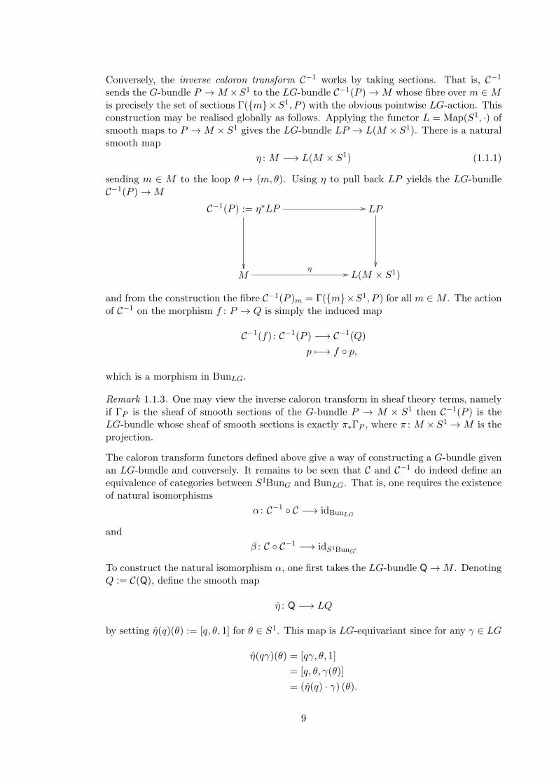
Conversely, the inverse caloron transform C−1 works by taking sections. That is, C−1

sends the G-bundle P →M ×S1 to the LG-bundle C−1(P )→M whose fibre over m ∈Mis precisely the set of sections Γ(m×S1, P ) with the obvious pointwise LG-action. Thisconstruction may be realised globally as follows. Applying the functor L = Map(S1, ·) ofsmooth maps to P →M × S1 gives the LG-bundle LP → L(M × S1). There is a naturalsmooth map

η : M −→ L(M × S1) (1.1.1)

sending m ∈ M to the loop θ 7→ (m, θ). Using η to pull back LP yields the LG-bundleC−1(P )→M

C−1(P ) := η∗LP LP

M L(M × S1)

//

η //

and from the construction the fibre C−1(P )m = Γ(m×S1, P ) for all m ∈M . The actionof C−1 on the morphism f : P → Q is simply the induced map

C−1(f) : C−1(P ) −→ C−1(Q)

p 7−→ f p,

which is a morphism in BunLG.

Remark 1.1.3. One may view the inverse caloron transform in sheaf theory terms, namelyif ΓP is the sheaf of smooth sections of the G-bundle P → M × S1 then C−1(P ) is theLG-bundle whose sheaf of smooth sections is exactly π∗ΓP , where π : M ×S1 →M is theprojection.

The caloron transform functors defined above give a way of constructing a G-bundle givenan LG-bundle and conversely. It remains to be seen that C and C−1 do indeed define anequivalence of categories between S1BunG and BunLG. That is, one requires the existenceof natural isomorphisms

α : C−1 C −→ idBunLG

and

β : C C−1 −→ idS1BunG.

To construct the natural isomorphism α, one first takes the LG-bundle Q→M . DenotingQ := C(Q), define the smooth map

η : Q −→ LQ

by setting η(q)(θ) := [q, θ, 1] for θ ∈ S1. This map is LG-equivariant since for any γ ∈ LG

η(qγ)(θ) = [qγ, θ, 1]

= [q, θ, γ(θ)]

= (η(q) · γ) (θ).

9

This gives the bundle map

Q LQ

M L(M × S1)

η //

η //

which, recalling the construction of C−1, defines an isomorphism αQ : C−1(C(Q)) → Qof LG-bundles. It is easy to see that for any morphism f : Q → P in BunLG one hasαP C−1(C(f)) = f αQ so that α is indeed a natural transformation from C−1 C toidBunLG .

To define the natural isomorphism β, first take any G-bundle P → M × S1. Since theconstruction of P := C−1(P ) is such that

Pm = Γ(m × S1, P ) (1.1.2)

for all m ∈M , it follows that the fibre of C(P) over (m, θ) ∈M × S1 is

(Pm × θ ×G)/LG =¶p : S1 → P | π p(θ) = (m, θ) for all θ ∈ S1

©× θ ×G

with π : P →M the projection. Then βP is the map

βP : [p, θ, g] 7−→ p(θ)g,

which is an isomorphism of G-bundles covering the identity. For any morphism f : P → Qin S1BunG, it is clear that βQ C(C−1(f)) = f βP so that β is a natural transformationfrom C C−1 to idS1BunG . This completes the proof of

Theorem 1.1.4 ([32, 33]). The caloron correspondence

C : BunLG −→ S1BunG and C−1 : S1BunG −→ BunLG

is an equivalence of categories that, for any manifold M , restricts to an equivalence ofgroupoids

C : BunLG(M) −→ S1BunG(M) and C−1 : S1BunG(M) −→ BunLG(M).

The following result establishes that the caloron correspondence truly is the bundle-theoretic version of the bijection c : f → f of (I.1).

Lemma 1.1.5. Take any G-bundle P → M × S1. If Uα is an open cover of M forwhich there are local sections sα ∈ Γ(Uα × S1, P ) then the LG-bundle P := C−1(P ) haslocal sections sα ∈ Γ(Uα,P).

Moreover, if ταβ are the transition functions of P with respect to the sections sα then thetransition functions of P with respect to the sections sα are precisely ταβ.

The converse is also true.

10

Proof. Since P is constructed by looping P , the map sα(m)(θ) := sα(m, θ) is a section ofP over Uα. Moreover, on the intersections Uαβ := Uα ∩ Uβ one has

sβ(m, θ) = sα(m, θ) · ταβ(m, θ) and sβ(m) = sα(m) · υαβ(m)

so evaluating the latter expression at θ ∈ S1 gives

υαβ(m)(θ) = ταβ(m, θ)

and hence υαβ = ταβ. The converse is essentially the above argument.

1.1.2 Higgs fields and connections

As mentioned previously, the true power of the caloron correspondence lies in its abilityto translate certain geometric data from loop group bundles to finite-dimensional bundlesand vice-versa. More specifically, there is a functorial equivalence between G-bundlesP → M × S1 equipped with a G-connection and LG-bundles Q → M equipped with anLG-connection and Higgs field (Definition 1.1.6).

Definition 1.1.6 ([32, 33]). A Higgs field on the LG-bundle Q → M is a smooth mapΦ: Q→ Lg that satisfies the twisted equivariance condition

Φ(qγ) = ad(γ−1)Φ(q) + γ−1∂γ (1.1.3)

for all q ∈ Q and γ ∈ LG, where ∂ denotes differentiation of the loop γ in the S1 direction.The space of Higgs fields HQ on a fixed LG-bundle Q→M is an affine space.

As a result of the caloron correspondence for bundles with connection, it will becomeapparent that Higgs fields really encode the S1 component of a connection on a G-bundleover M × S1. The following result guarantees the existence of Higgs fields on any LG-bundle Q→M .

Lemma 1.1.7 ([33, 41]). Higgs fields exist.

Proof. It is evident that a convex combination of Higgs fields is again a Higgs field andthat any trivial LG-bundle admits the trivial Higgs field

LG −→ Lg

γ 7−→ γ−1∂γ.

The result follows by choosing a smooth partition of unity for M subordinate to a giventrivialisation.

Having established this result, one is almost in a position to describe the geometric caloroncorrespondence.

Definition 1.1.8. Let S1BuncG to be the category whose objects are objects of S1BunG

equipped with G-connections and whose morphisms are the connection-preserving mor-phisms of S1BunG.

For a fixed manifold M , define S1BuncG(M) to be the groupoid with objects the G-bundles

P → M × S1 equipped with connection, with morphisms those connection-preservingbundle maps covering the identity.

11

Moreover, in the case that the group is a loop group, define BuncLG to be the categorywhose objects are LG-bundles equipped with LG-connections and Higgs fields. Morphismsof this category are LG-bundle maps that preserve the additional structure. For a fixedmanifold M , the groupoid BuncLG(M) is defined similarly to the above.

To define the geometric caloron transform, a functor

C : BuncLG −→ S1BuncG,

first take the LG-bundle Q → M equipped with LG-connection A and Higgs field Φ.Define the 1-form A on Q× S1 ×G by

A(q,θ,g) := ad(g−1)ÄAq(θ) + Φ(q)(θ)dθ

ä+ Θg, (1.1.4)

with Θ the Maurer-Cartan form on G.

Lemma 1.1.9 ([32, 33, 41]). The 1-form A defined by equation (1.1.4) descends to aG-connection, also called A, on the caloron transform Q := C(Q) = (Q× S1 ×G)/LG.

Proof. The proof is essentially that of [33, Proposition 3.9]. To show that equation (1.1.4)determines a well-defined 1-form on C(Q), one must show that it is basic for the projectionQ× S1 ×G→ C(Q).

Take any X ∈ T[q,θ,g]Q and suppose that X, X ′ are lifts of the vector X to Q × S1 × G.Without loss of generality, one may suppose that

X ∈ T(q,θ,g)(Q× S1 ×G) and X ′ ∈ T(q,θ,g)γ(Q× S1 ×G).

Since X and X ′ are both lifts of X, one has that the pushforward dRγX of X by the (right)action Rγ of γ satisfies dRγX = X ′+V for some vertical vector V . It is therefore sufficientto show that A is invariant under the LG-action and that it annihilates vertical vectors.For simplicity of calculation, one supposes G to have a faithful matrix representation1 sothat the exponential map may be written as exp(tξ) = 1 + tξ +O(t2). Thus any verticalvector at (q, θ, g) is of the form

V =d

dt

(q, θ, g) · exp(tξ)

t=0

=Äξ#q , 0,−ξ(θ)g

äfor some ξ ∈ Lg, where ξ# is the fundamental vector field on Q generated by ξ. The actionof A on such a vector is

A(q,θ,g)(V ) = ad(g−1)(ξ(θ))− g−1ξ(θ)g = 0.

To see that A is basic suppose that

X(q,θ,g) =d

dt

Äγχ(t), θ + tx, g exp(tζ)

ät=0

= (χ, x, gζ).

Then for γ ∈ LG, the pushforward dRγ(X) is given by

dRγ(X)(q,θ,g)γ =d

dt

Äγχ(t)γ, θ + tx, γ(θ + tx)−1g exp(tζ)

ät=0

=ÄdRγ(χ), x, γ(θ)−1g

îζ − x ad(g−1)(∂γ(θ))γ(θ)−1

óä.

1since this thesis deals exclusively with G a compact Lie group or G = GLn(C) for some n, thisassumption is not restrictive. This assumption is not required in the general case.

12

Consequently,

R∗γA(q,θ,g)(X) = A(qγ,θ,γ(θ)−1g)(dRγ(X))

= ad(g−1γ(θ))Äad(γ(θ)−1)Aq(χ)(θ) + x ad(γ(θ)−1)Φ(q)(θ) + xγ(θ)−1∂γ(θ)

ä+ ζ − x ad(g−1)(∂γ(θ))γ(θ)−1

= ad(g−1) (Aq(χ)(θ) + xΦ(q)(θ)) + ζ

= A(q,θ,g)(X).

This shows that the 1-form defined in (1.1.4) does indeed descend to a form on Q, whichshall also be called A.

To see that A is a G-connection, one must show that it reproduces the Lie algebra gener-ators of fundamental vector fields on Q and that it is equivariant for the G-action. Noticethat the vertical vector generated by ξ ∈ g at [q, θ, g] ∈ Q is

V =d

dt

îq, θ, g exp(tξ)

ót=0

= [0, 0, gξ]

so that A[q,θ,g](V ) = ξ as required. It remains only to show that R∗hA(X) = ad(h−1)A(X)for all h ∈ G and vector fields X. If X = [χ, x, gξ] ∈ T[q,θ,g]Q then

R∗hA[q,θ,g](X) = A[q,θ,gh]([χ, x, gh ad(h)−1ξ])

= ad(h−1g−1) (Aq(χ)(θ) + xΦ(q)(θ)) + ad(h−1)ξ

= ad(h−1)A[q,θ,g](X)

which completes the proof.

Having this result, one defines the geometric caloron transform of the LG-bundle Q→Mwith LG-connection A and Higgs field Φ as the G-bundle C(Q) → M × S1 equippedwith the connection A determined by (1.1.4). Since a morphism f : Q → P in BuncLGis required to respect the geometric data, the expression (1.1.4) and the definition of Ctogether imply that the G-bundle morphism C(f) : C(Q) → C(P) as defined previouslyrespects the connective data and so is a morphism of S1Bun

cG.

To define the geometric inverse caloron transform, a functor

C−1 : S1BuncG −→ BuncLG,

first take a G-bundle P → M × S1 with connection A. Recalling that P := C−1(P ) isdefined essentially by looping P , one defines the LG-connection A on P via the expression

Aq(χ)(θ) := Aq(θ)(χ(θ)), (1.1.5)

as the tangent vector χ ∈ TqP is naturally equivalent to a section of the pullback vectorbundle q∗TP → S1 (see [20, Example 4.3.3] or Appendix A). It is immediate that Asatisfies the properties required of an LG-connection simply by virtue of the fact that Ais a connection.

Writing ∂ for the canonical vector field on S1, one defines a Higgs field Φ on P via theexpression

Φ(q)(θ) := q∗Aθ(∂). (1.1.6)

13

To see that Φ satisfies the twisted equivariance condition (1.1.3), take γ ∈ LG so that

Φ(qγ)(θ) = (qγ)∗Aθ(∂)

= Aq(θ)γ(θ)

ÄdRγ(θ)(∂q(θ)) + (γ(θ)−1∂γ(θ))#

ä= ad(γ(θ)−1)Φ(q)(θ) + γ(θ)−1∂γ(θ)

as required. Notice that this formulation justifies the remark following Definition 1.1.6,since the Higgs field constructed above really is the S1 component of the connection A.

The geometric inverse caloron transform is given by sending the G-bundle P → M × S1

with G-connection A to the LG-bundle C−1(P )→M with the LG-connection A and Higgsfield Φ given by (1.1.5) and (1.1.6) respectively. As for C, the action of C−1 on morphismsis straightforward by virtue of the fact that morphisms in S1Bun

cG necessarily preserve

the connective data.

Theorem 1.1.10 ([32, 33]). The geometric caloron correspondence

C : BuncLG −→ S1BuncG and C−1 : S1Bun

cG −→ BuncLG


C : BuncLG(M) −→ S1BuncG(M) and C−1 : S1Bun

cG(M) −→ BuncLG(M).

Proof. It suffices to show that the natural isomorphisms βP and αQ of Theorem 1.1.4preserve the connective data. If one starts with the LG-bundle Q → M with connectionA and Higgs field Φ then the connection A′ on Q′ := C−1(C(Q)) is given by

A′q(χ)(θ) := Aq(θ)(χ(θ))

where Q := C(Q) is equipped with caloron-transformed connection A. Recall that thenatural isomorphism αQ : C−1(C(Q))→ Q satisfies

α−1Q (q) :=

Äθ 7→ [q, θ, 1]

äso that

(α−1Q )∗A′q(χ)(θ) = A[q,θ,1]([χ, 0, 0]) := Aq(χ)(θ).

Thus αQ preserves the LG-connections and an analogous argument holds for the Higgsfields.

On the other hand, if one begins with a G-bundle P → M × S1 with connection A, thenthe connection A′ on P ′ := C(C−1(P )) is given by

A′[p,θ,g] = ad(g−1)ÄAp(θ) + Φ(p)(θ)dθ

ä+ Θg,

with A and Φ repsectively the connection and Higgs field on the (inverse) caloron transformP := C−1(P ) of P . Recall that βP is given by sending

[p, θ, g] 7−→ p(θ)g,

so considering the tangent vector

X[p,θ,g] =d

dt

îγχ(t), θ + tx, g exp(tζ)

ót=0

= [χ, x, ζ]

14

one obtains

dβP (X)p(θ)g =d

dt

γχ(t)(θ + tx)g exp(tζ)

t=0

= χ(θ)g + x ∂p(θ)g + ζ#p(θ)g.

Hence

β∗PA[p,θ,g](X) = ad(g−1)ÄAp(θ)(χ(θ)) + xAp(θ)(∂p(θ))

ä+ ζ = A′[p,θ,g](X).

This completes the proof.

1.1.3 String classes

The enhanced caloron correspondence of Theorem 1.1.10 turns out to be a very usefultool, particularly for constructing characteristic classes for LG-bundles. The procedure isa relatively simple variation of the standard Chern-Weil theory and relies on the calorontransform and integration over the fibre (cf. Appendix B).

First, one recalls briefly the theory of characteristic classes; classical references for thismaterial are [29, 39]. For any Lie group G there is a universal G-bundle EG → BGsuch that the total space EG is contractible. A key property of the universal bundleis that for any (topological) G-bundle P → M there is a classifying map f : M → BGsuch that the pullback f∗EG is isomorphic to P . The homotopy class of the classifyingmap f is uniquely determined by P and for any two homotopic maps f0, f1 : M → BGthe pullbacks f∗0EG and f∗1EG are isomorphic as G-bundles over M . This establishesa bijective correspondence between principal G-bundles over M and homotopy classes ofmaps M → BG. It is important to notice that in general neither EG or BG are assumedto be smooth manifolds and that they are unique only up to homotopy equivalence.

A characteristic class associates to a G-bundle P →M a class c(P ) in the cohomology ofM that is natural in the sense that if f : N →M is a continuous (or, in the setting of thecaloron correspondence, smooth) map then f∗c(P ) = c(f∗(P )). Since all G-bundles arepullbacks of the universal G-bundle EG→ BG, characteristic classes correspond preciselywith cohomology classes of BG.

One important method for manufacturing characteristic classes is Chern-Weil theory. Let

g⊗k := g⊗ · · · ⊗ g︸︷︷︸k times

,

then an invariant polynomial of degree k on g is a symmetric multilinear map g⊗k → Rthat is invariant under the adjoint action of G on g⊗k. The set of invariant polynomialsof degree k is denoted Ik(g). Invariant polynomials multiply in a natural way so thatI•(g) =

⊕∞i=1 I

k(g) is a graded algebra.

Denote by Ωp(M ; g⊗q) the space of differential p-forms on M taking values in g⊗q. Thereis a wedge product ∧ : Ωp(M ; g⊗q)× Ωp′(M ; g⊗q

′)→ Ωp+p′(M ; g⊗q+q

′) given by

α ∧ β (X1, . . . , Xp+p′) :=∑

σ∈Sp+p′(−1)|σ|α

ÄXσ(1), . . . , Xσ(p)

ä⊗ βÄXσ(p+1), . . . , Xσ(p+p′)

äfor vector fields X1, . . . , Xp+p′ on M , where Sk is the group of permutations on 1, . . . , kand |σ| is the sign of the permutation σ. If α ∈ Ωp(M ; g) and β ∈ Ωp′(M ; g) set

[α, β](X1, . . . , Xp+p′) :=∑

σ∈Sp+p′(−1)|σ|

îαÄXσ(1), . . . , Xσ(p)

ä, βÄXσ(p+1), . . . , Xσ(p+p′)

äó15

and there is also an exterior derivative d : Ωp(M ; g⊗q) → Ωp+1(M ; g⊗q). If f ∈ Ik(g) andωi ∈ Ωpi(M ; g) for i = 1, . . . , k write

f(ω1, . . . , ωk) := f(ω1 ∧ · · · ∧ ωk) ∈ Ωp1+···+pk(M).

The ad-invariance of f implies

k∑i=1

(−1)(p1+···+pi)f(ω1, . . . , [ωi, $], . . . , ωk) = 0

for any $ ∈ Ω1(M ; g) (cf. [11] or [41, Lemma 3.2.6] for the case that $ has degree p ≥ 1).The following is well-known

Theorem 1.1.11 (Chern-Weil Homomorphism). Given a G-bundle P →M with connec-tion A and curvature F , for any f ∈ Ik(g) the real-valued 2k-form

cwf (A) := f(F, . . . , F︸︷︷︸k times

)

on P is closed and descends to a form on M whose class in de Rham cohomology isindependent of the choice of connection A. Using the de Rham isomorphism, this definesa map

cw : I•(g) −→ H2•(M ;R),

which is an algebra homomorphism.

For a detailed treatment of Chern-Weil theory, including a proof of this result, see [12]. Animmediate consequence is that the cohomology class of cwf (A) gives a characteristic classcwf (P ) ∈ H2k(M ;R) for any f ∈ Ik(g). By a result of H. Cartan [9], if G is compact thenall characteristic classes for G-bundles in R-valued cohomology are Chern-Weil classes (seealso [12, Theorem 8.1]).

In a similar vein, one may use the caloron correspondence and the Chern-Weil homo-morphism to construct characteristic classes for LG-bundles; classes constructed in thismanner are called string classes. To construct the string classes of the LG-bundle Q→M ,choose any LG-connection A and Higgs field Φ on Q. Applying the caloron transform givesthe G-bundle Q→M × S1 equipped with the G-connection A.

Definition 1.1.12 ([33, 41]). The string form associated to f ∈ Ik(g) is

sf (A,Φ) :=

∫S1cwf (A), (1.1.7)

which is a closed (2k − 1)-form on M . The operation∫S1 here denotes integration over

the fibre of differential forms (see Appendix B).

Since the exterior derivative commutes with integration over the fibre (Lemma B.1.5)Theorem 1.1.11 implies that the cohomology class of sf (A,Φ) depends neither on the LG-connection A nor on the Higgs field Φ—this can also be seen immediately as a result ofthe construction of the string potential forms in Chapter 2, in particular Theorem 2.1.8.Therefore, taking the cohomology class and applying the de Rham isomorphism gives thestring class

sf (Q) ∈ H2k−1(M ;R), (1.1.8)

16

which is a characteristic class for any f ∈ Ik(g).

This construction of the string classes naturally provides differential form representativesthat seem to depend on data on the caloron transform. However, the caloron correspon-dence allows one to write these representatives entirely in terms of data on the underlyingLG-bundle. Namely, given the LG-bundle Q → M with connection A and Higgs field Φ,let Q := C(Q) be its caloron transform with caloron-transformed connection A. The stringform associated to the invariant polynomial f ∈ Ik(g) is then

sf (A,Φ) =

∫S1f(F, . . . , F︸︷︷︸

k times

)

with F the curvature of the connection A on Q. Recall F = dA+ 12 [A,A] and that, in this

case, the connection A is given by (1.1.4) so one may write F in terms of A and Φ; firstnotice that

[A,A] =îad(g−1) (A + Φdθ) + Θ, ad(g−1) (A + Φdθ) + Θ

ó= ad(g−1) ([A,A] + 2[A,Φ] ∧ dθ) + 2[Θ, ad(g−1)A] + 2[Θ, ad(g−1)Φ] ∧ dθ.

Recall also that dω(X,Y ) := X(ω(Y ))− Y (ω(X))− ω([X,Y ]) for a 1-form ω and vectorfields X,Y . If X and Y are the vector fields on Q whose values at the point [q, θ, g] ∈ Qare

X[q,θ,g] =d

dt

Äγχ(t), θ + tx, g exp(tζ)

ät=0

= (χ, x, gζ)

Y[q,θ,g] =d

dt

Äγκ(t), θ + ty, g exp(tξ)

ät=0

= (κ, y, gξ)

then

[X,Y ][q,θ,g] = ([χ, κ], 0, g[ζ, ξ]).

First, one calculates d(ad(g−1)A) by noticing that at the point [q, θ, g]

XÄ

ad(g−1)A(Y )ä

=d

dt

(1− tζ)g−1Aγχ(t)(Y )(θ + tx)g(1 + tζ)

t=0

=d

dt

ad(g−1)Aγχ(t)(κ)(θ)

t=0

+ x ad(g−1)∂Aq(κ)(θ)

−îζ, ad(g−1)Aq(κ)(θ)

óand hence

d(ad(g−1)A) = ad(g−1)dA + ∂A ∧ dθ −îΘ, ad(g−1)A

ó,

where ∂A is the Lg-valued 1-form on Q given by differentiating A in the S1 direction.

Applying the same argument to ad(g−1)Φ dθ this all gives

d(ad(g−1)Φdθ) = ad(g−1)dΦ ∧ dθ −îΘ, ad(g−1)Φ

ó∧ dθ,

so recalling that the Maurer-Cartan form Θ satisfies dΘ + 12 [Θ,Θ] = 0 gives

F = ad(g−1)

ÅdA +

1

2[A,A] + (dΦ + [A,Φ]− ∂A) ∧ dθ

ã.

17

Writing F = dA + 12 [A,A] for the curvature of A and defining the Higgs field covariant

derivative2 ∇Φ := dΦ + [A,Φ]− ∂A, one obtains

F = ad(g−1)(F +∇Φ ∧ dθ). (1.1.9)

Using the properties of f ∈ Ik(g) yields the expression

sf (A,Φ) = k

∫S1f(∇Φ, F, . . . ,F︸︷︷︸

k − 1 times

) (1.1.10)

for the string form associated to f . Note that the integration symbol in (1.1.10) denotesthe standard integration operation on functions S1 → R and not integration over the fibre.

Example 1.1.13. In [27] Killingback studied the notion of a string structure, which is thestring-theoretic analogue of a spin structure. If G is a compact, simple, simply-connectedLie group then it is well-known (see [36], for example) that there is a universal centralextension

0 −→ S1 −→ LG −→ LG −→ 0

of the loop group LG. A string structure on M is then given by a lifting of the LG-bundleQ→M to an LG-bundle “Q→M and there is an integral three-class—the original stringclass—that measures the obstruction to such a lift. Using the machinery of bundle gerbes,which give smooth geometric representatives for degree three integral cohomology throughtheir Dixmier-Douady classes, Murray and Stevenson [32] gave an explicit formula for ade Rham representative of this class, namely

− 1

4π2

∫S1〈∇Φ,F〉.

In this expression, F and ∇Φ are respectively the curvature of a connection and covariantderivative of a Higgs field on Q and 〈·, ·〉 is the Killing form on g normalised so that thelongest root has length

√2. It is clear that this string class is simply the string class (in

the sense of (1.1.8)) corresponding to the ad-invariant polynomial

f(·, ·) := − 1

8π2〈·, ·〉.

Notice in particular that if Q is the caloron transform of Q equipped with the caloron-transformed connection A then

sf (Q) =

∫S1p1(Q)

where p1(Q) is the first Pontryagin class of Q.

1.2 The based case

In Section 1.1, the main objects under consideration were LG-bundles over M and thecorresponding G-bundles over M × S1. It turns out that with a little more work, one

2one might be tempted to call ∇Φ the ‘Higgs field curvature’, however there is a generalised version ofthe caloron correspondence in which an additional term FΦ appears on the right-hand side of the expression(1.1.9) [25, pp. 238]. In this context it is more appropriate to call FΦ the Higgs field curvature, so thisterminology is used here for consistency.

18

may extend all of the results of Section 1.1 to give a caloron correspondence for principalbundles whose structure group is the based loop group

ΩG := γ ∈ LG | γ(0) = 1,

a Frechet Lie subgroup of LG. The key innovation here is the use of framings (Definition1.2.1) on the finite-dimensional side to reduce the structure group on the Frechet side fromLG to ΩG. The discussion presented here is largely based off of [33, 41].

Definition 1.2.1. Let P → X be a G-bundle and X0 ⊂ X a submanifold. Then P isframed over X0 if there is a distinguished section s0 ∈ Γ(X0, P ). Write P0 = s0(X0) ⊂ Pfor the image of s0.

In what follows, if P →M × S1 is a G-bundle then, unless stated otherwise, the framingshall be taken over the submanifold M0 := M × 0.

Definition 1.2.2. Define frBunG to be the category whose objects are framed G-bundlesP → M × S1 and whose morphisms are G-bundle maps that preserve the framings andcover a map of the form f × id : N × S1 →M × S1.

For a fixed manifold M , let frBunG(M) be the groupoid with objects the framed G-bundlesP →M ×S1 with morphisms those bundle maps preserving the framing and covering theidentity on M × S1.

The based caloron transform is then the functor

C : BunΩG −→ frBunG

constructed as in Section 1.1.1, i.e. by sending the ΩG-bundle Q → M to the associatedbundle

C(Q) := (Q× S1 ×G)/ΩG.

This bundle has a canonical framing given by

s0(m, 0) := [q, 0, 1],

where q is any point in the fibre of Q over m, and so is an object of frBunG. The actionof C on morphisms is given analogously to the free loop case, noting of course that iff : Q → P is a morphism in BunΩG, then C(f) : C(Q) → C(P) preserves the framings andtherefore gives a morphism in frBunG.

Conversely, the based inverse caloron transform is a functor

C−1 : frBunG −→ BunΩG .

defined similary to the free loop case, i.e. by first looping and then pulling back by themap η of (1.1.1). The distinction here is that instead of applying the smooth loop functorL = Map(S1, ·) to the framed G-bundle P → M × S1 one takes based loops. If X is asmooth (finite-dimensional) manifold with submanifold X0 ⊂ X, define the based loopmanifold

ΩX0X := p : S1 → X smooth | p(0) ∈ X0.

The based inverse caloron transform is given by first taking the based loop bundle

ΩP0P −→ ΩM0(M × S1),

19

which is an ΩG-bundle, and then pulling back by η to obtain the ΩG-bundle C−1(P )→M .The action of C−1 on morphisms is defined similarly to the free loop case and, as before,

Theorem 1.2.3 ([33, 41]). The based caloron correspondence

C : BunΩG −→ frBunG and C−1 : frBunG −→ BunΩG


C : BunΩG(M) −→ frBunG(M) and C−1 : frBunG(M) −→ BunΩG(M).

Proof. The natural isomorphisms α and β are constructed in an analogous fashion to thenatural isomorphisms of Theorem 1.1.4 and, following the arguments presented there, areeasily seen to satisfy the required properties.

As in the free loop case, there is an extension of the based caloron correspondence tobundles with connection. In this setting, connections on the G-bundle side are requiredto satisfy a compatibility condition with respect to the framings.

Definition 1.2.4. Let P → X be a framed G-bundle with framing s0 ∈ Γ(X0, P ). Aconnection A on P is framed (with respect to s0) if s∗0A = 0.

This framing condition is required to guarantee that the connections constructed on theFrechet side are indeed valued in Ωg = Lie(ΩG). Framed connections exist on framedbundles provided, as is assumed in this thesis, that the base manifold admits smoothpartitions of unity [33, Lemma 3.5].

Definition 1.2.5. Let frBuncG to be the category whose objects are objects of frBunGequipped with framed G-connections and whose morphisms are the connection-preservingmorphisms of frBunG.

For a fixed manifold M , frBuncG(M) denotes the groupoid with objects the framed G-bundles P →M×S1 equipped with framed connection and with morphisms the connection-preserving bundle maps covering the identity that also preserve the framing.

In order to formulate the geometric caloron correspondence for based loop group bundles,one requires the correct notion of Higgs field for ΩG-bundles. It turns out that this isgiven exactly by replacing LG in Definition 1.1.6 by ΩG.

Remark 1.2.6. Higgs fields on ΩG-bundles still map into Lg, not Ωg as one might suspect.This is because in general γ−1∂γ /∈ Ωg for γ ∈ ΩG, so a Higgs field cannot both map intoΩg and satisfy the twisted equivariance condition.

Lemma 1.1.7 may be easily adapted to show that every ΩG-bundle admits a Higgs field.

Define the categories BuncΩG and BuncΩG(M) exactly as in Definition 1.1.8 (with LGreplaced by ΩG). The based geometric caloron transform is the functor

C : BuncΩG −→ frBuncG

defined by sending the ΩG-bundle Q → M with ΩG-connection A and Higgs field Φ tothe framed G-bundle C(Q)→M × S1 (as defined above) equipped with the connection A

20

given by the expression (1.1.4). To see that this is well-defined, one must verify that theconnection A is framed. Recall that the framing of C(Q) is the section

s0 : (m, 0) 7−→ [q, 0, 1].

Therefore, taking any X ∈ T(m,0)M0 (so that ds0(X) = [χ, 0, 0] for some tangent vector χto Q), one obtains

s∗0A(m,0)(X) = A[q,0,1]([χ, 0, 0]) = Aq(χ)(0) = 0

since A is valued in Ωg. The action of C on morphisms is essentially the same as in thefree loop case.

Conversely, the based inverse geometric caloron transform is a functor

C−1 : frBuncG −→ BuncΩG

sends the framed G-bundle P → M × S1 with framed connection A to an ΩG-bundleP → M equipped with ΩG-connection A and Higgs field Φ. Here P := C−1(P ) is thebased inverse caloron transform as above and the connection A and Higgs field Φ are givenrespectively by (1.1.5) and (1.1.6). Since it is clear that Φ is well-defined, the only thingthat needs to be shown is that the connection A is indeed an ΩG-connection. To see this,take any χ ∈ TpP noting that χ(0) ∈ Tp(0)P0 is in the image of the map ds0 : TM0 → TP0.Thus

Ap(χ)(0) = Ap(0)(χ(0)) = s∗0A(m,0)(X) = 0

where p(0) is in the fibre of P over (m, 0) and ds0(X) = χ(0). Once again, the action ofC−1 on morphisms is essentially the same as in the free loop case.

One may verify that the natural isomorphisms of Theorem 1.2.3 respect the connectivedata, the arguments proceeding exactly as in the free loop case, so that

Theorem 1.2.7 ([33, 41]). The based geometric caloron correspondence

C : BuncΩG −→ frBuncG and C−1 : frBuncG −→ BuncΩG


C : BuncΩG(M) −→ frBuncG(M) and C−1 : frBuncG(M) −→ BuncΩG(M).

1.2.1 The path fibration and string classes

The argument that constructed the string classes of Section 1.1.3 may easily be adaptedin order to construct characteristic classes for ΩG-bundles, which are also called stringclasses.

Explicitly, for an ΩG-bundle Q → M equipped with connection A and Higgs field Φ andfor any invariant polynomial f ∈ Ik(g), one obtains the closed string form

sf (A,Φ) = k

∫S1f(∇φ, F, . . . ,F︸︷︷︸

k − 1 times

)

21

noticing that this is exactly the expression (1.1.10)—the only thing that has changed isthat the connection and Higgs field now live on an ΩG-bundle. As in the free loop case,the corresponding class in the real-valued cohomology of M is the string class

sf (Q) ∈ H2k−1(M ;R),

which is independent of the choice of A and Φ.

So far, there have not been any particularly novel features of the based case. One advantageof working with based loops instead of free loops is that there is a smooth model forthe universal ΩG-bundle—the path fibration—that allows one to explicitly compute theuniversal string classes.

ΩG PG

G

//

ev2π

Let PG be the space of all smooth maps p : R → G such that p(0) is the identity andp−1∂p is periodic with period 2π. There is a natural action of ΩG on PG that gives PGthe structure of an ΩG-bundle over G. The projection PG → G is simply evaluation ofpaths at 2π and it turns out that PG is (smoothly) contractible. Therefore PG→ G is amodel for the universal ΩG-bundle, which also shows that BΩG = G in this case. For arigorous treatment see Appendix A.

Since PG is a smooth manifold one may talk about connective data directly on the uni-versal ΩG-bundle. Recall that a tangent vector χ ∈ TpPG is canonically identified with asection of p∗TG→ R so that a vertical vector for PG→ G is a tangent vector such that

χ(2π) = 0.

Choosing a smooth function α : R → R satisfying α(t) = 0 for t ≤ 0 and α(t) = 1 fort ≥ 2π, a complementary horizontal subspace at p ∈ PG is given by

Hp = χ ∈ TpPG | χ(θ) = α(θ)dRp(θ)(ξ) for some ξ ∈ g

(see also [32, pp. 552–553]). The horizontal projection of any tangent vector χ ∈ TpPG is

χh(θ) = α(θ)dRp(2π)−1p(θ) (χ(2π)) .

and the value of the ΩG-connection corresponding to this splitting of the tangent bundleat p ∈ PG is

A∞(θ) = Θ(θ)− α(θ) adÄp(θ)−1

äev∗2π

“Θwith Θ the Maurer-Cartan form on ΩG3 and “Θ the right-invariant Maurer-Cartan formon G. There is a canonical Higgs field on PG given by

Φ∞(p) = p−1∂p

3given by Θγ(ξ)(θ) := (ΘG)γ(θ)(ξ(θ)) where γ ∈ ΩG, ξ ∈ TγΩG and ΘG momentarily denotes theMaurer-Cartan form on G.

22

and some straightforward calculations (as in [41, Section 3.1.2]) show that

F∞ = −1

2α(1− α) ad(p−1) ev∗2π

Ä[“Θ,“Θ]

äand ∇Φ∞ =

dα

dθad(p−1) ev∗2π

Ä“Θä. (1.2.11)

Assuming a fixed choice of smooth function α, A∞ and Φ∞ are respectively the standardconnection and Higgs field for PG.

One is now in a position to explicitly calculate the universal string forms, which are odd-degree forms on G, as follows. Taking any f ∈ Ik(g) gives

Lemma 1.2.8 ([33, 41]). The string form of the standard connection and Higgs field ofthe path fibration over G is

τf :=

Å−1

2

ãk−1 k!(k − 1)!

(2k − 1)!fÄΘ, [Θ,Θ], . . . , [Θ,Θ]︸︷︷︸

k − 1 times

äwith Θ the Maurer-Cartan form on G.

Proof. Plugging the expressions from (1.2.11) into the formula (1.1.10) and using the factthat Θg = ad(g−1)“Θg gives

sf (A∞,Φ∞) = k

Å−1

2

ãk−1 Å∫S1αk−1(1− α)k−1dα

dθdθ

ãfÄΘ, [Θ,Θ], . . . , [Θ,Θ]︸︷︷︸

k − 1 times

ä.

The integral is evaluated as∫S1αk−1(1− α)k−1dα

dθdθ =

∫ 1

0tk−1(1− t)k−1 dt =

(k − 1)!(k − 1)!

(2k − 1)!

using the beta function, which completes the proof.

Remark 1.2.9. The de Rham cohomology classes of the forms τf appearing in Lemma1.2.8 are well-known (cf. [11, 24]) to be precisely the cohomology classes on G obtainedby transgressing classes on BG. H•(G;R) is generated as an exterior algebra by (finitelymany) such transgressed classes [2, Theorem 18.1].

Another major advantage that comes from working with based loop group bundles is thatclassifying maps are easy to describe. Namely, given an ΩG-bundle Q → M a choice ofHiggs field Φ on Q is equivalent to choosing a smooth classifying map M → G for Q inthe following manner. At the point q ∈ Q the equation

Φ(q) = g(q)−1∂g(q) (1.2.12)

for g = g(q) ∈ PG has a unique solution by the Picard-Lindelof Theorem. The holonomyof the Higgs field Φ is then the map holΦ : Q→ PG that sends

q 7−→ holΦ(q) := g

with g satisfying (1.2.12). As Φ is smooth, holΦ is also smooth and notice also that holΦis ΩG-equivariant, for if γ ∈ ΩG and g = holΦ(q) then

(gγ)−1∂(gγ) = ad(γ−1)g−1∂g + γ−1∂γ = Φ(qγ)

implies that holΦ(qγ) = holΦ(q)γ. Hence holΦ descends to a map M → G, which shallalso be called holΦ, proving

23

Proposition 1.2.10 ([33]). If Q → M is an ΩG-bundle and Φ is any Higgs field on Qthen holΦ : M → G is a smooth classifying map for Q.

Writing

τ : I•(g) −→ H2•−1(G;R)

for the map f 7→ [τf ], with τf the forms of Lemma 1.2.8, by naturality of the string classesand using (1.1.7) one obtains

Theorem 1.2.11 ([33]). If Q→M is an ΩG-bundle and

s(Q) : I•(g) −→ H2•−1(M ;R)

is the map f 7→ sf (Q) then the diagram

I•(g) H2•(M × S1;R)

H2•−1(G;R) H2•−1(M ;R)

cw(Q) // ”∫S1

τ

s(Q)

''hol∗Φ //

commutes for any choice of Higgs field Φ on Q, where Q := C(Q) is the caloron transform.

Here∫S1 : H•(M × S1;R)→ H•−1(M ;R) is the integration over the fibre map in singular

cohomology.

An immediate consequence of this is that for any choice of connection A and Higgs fieldΦ on Q there is some (2k − 2)-form ω on M such that

sf (A,Φ) = hol∗Φ τf + dω.

As shown in Proposition 1.2.14 below, for each choice of A and Φ there is a correspondingcanonical choice of ω. The fact that there is a canonical choice of ω plays an important rolein relating the Ω model of Chapter 4 to the TWZ differential extension of odd K-theoryin Section 4.2.1.

It is important for the construction of these canonical forms to understand how the Higgsfield holonomy is related to the conventional notion of holonomy of a connection. Firsttake a G-bundle π : P → X with framing s0 over X0 and framed connection A. WritingP0 = s0(X0) as before and taking based loops4 gives the ΩG-bundle ΩP0P → ΩX0X, asin the construction of the based inverse caloron transform functor. Take a loop p ∈ ΩP0Pand project down to ΩX0X to obtain π p. Taking the horizontal lift p of π p throughs0(π p(0)) with respect to the connection A, one has

p = phol(p)

for some hol(p) ∈ PG. Notice that hol is ΩG-equivariant since pγ = p for each γ ∈ ΩGand so

pγ = pγ hol(pγ) =⇒ hol(pγ) = hol(p)γ.

4recalling that, for example, ΩX0X = γ ∈ LX | γ(0) ∈ X0.

24

Thus, hol descends to a map hol : ΩX0X → G such that the diagram

ΩP0P PG

ΩX0X G

hol //

hol //

commutes. In particular, hol is a classifying map for ΩP0P and agrees with the traditionalnotion of holonomy (see also [8, Section 3]). Recalling the map η : M → ΩM0(M × S1) of(1.1.1) used in the definition of the caloron correspondence one has

Lemma 1.2.12 ([33, 41]). Let Q → M be an ΩG-bundle with connection A and Higgsfield Φ. Write Q→M×S1 for its caloron transform, with the framed connection A. Thenthe Higgs field holonomy is related to the usual holonomy (with respect to A) by

holΦ = hol η.

For a proof of this fact see [41, Lemma 3.1.1]. In [41, Lemma 3.1.2] it is also shown that5

Lemma 1.2.13 ([41]). For differential k-forms on M × S1

η∗∫S1

ev∗ =

∫S1

where ev : ΩM0(M × S1)× S1 →M × S1 is the evaluation map (γ, θ) 7→ γ(θ).

With these results, one is able to prove

Proposition 1.2.14. Let Q → M be an ΩG-bundle. For any f ∈ Ik(g), and choice ofΩG-connection A and Higgs field Φ on Q, there is a canonical choice of (2k − 2)-form χon M such that

sf (A,Φ) = hol∗Φ τf + dχ.

Proof. The proof is essentially that of [41, Proposition 3.2.7] and [33, Proposition 4.15].Let Q → M × S1 be the caloron transform, with framing s0 ∈ Γ(M0, Q) and framedconnection A. Pulling back by the evaluation map ev : ΩM0(M × S1) × [0, 1] → M × S1

one obtains the G-bundle ev∗Q → ΩM0(M × S1) × [0, 1]. This bundle is in fact trivial,since it has a section

h : ΩM0(M × S1)× [0, 1] −→ ev∗Q

given by h(p, t) := p(t), where p is the horizontal lift of p through s0(p(0)) with respect tothe connection A on Q. Setting “A := h∗ ev∗A,

since ΩM0(M × S1)× [0, 1] is a product manifold one may write

h∗ ev∗ F = − ∂

∂t“A ∧ dt+ “F = −∂t“A ∧ dt+ “F

5in fact, the argument presented there proves this only for the case k = 4 but the argument is sufficientlygeneral to hold for all k.

25

where F is the curvature of A and, if ςt : p 7→ (p, t) is the slice map, ς∗t“F is the curvature

of ς∗t“A.

Putting this aside for one moment, considering the Chern-Weil forms on M × S1 one has

sf (A,Φ) =

∫S1cwf (A) = η∗

∫S1

ev∗ cwf (A) = η∗∫S1cwf (ev∗A)

for any f ∈ Ik(g) by Lemma 1.2.13. Inserting the above expression for h∗ ev∗ F andtreating S1 as [0, 1] with endpoints identified6 gives

cf :=

∫S1cwf (ev∗A) = −k

∫ 1

0fÄ∂t“A, “F , . . . , “F︸︷︷︸

k − 1 times

ädt.

Using the formula “F = d“A+ 12 [“A, “A], this becomes

cf = −kk−1∑i=0

1

2i(k − 1)!

i!(k − 1− i)!

∫ 1

0fÄ∂t“A, d“A, . . . , d“A︸︷︷︸

k − 1− i times

, [“A, “A], . . . , [“A, “A]︸︷︷︸i times

ädt

For i = 0, . . . , k − 1 set

fi := fÄ∂t“A, d“A, . . . , d“A︸︷︷︸

k − 1− i times

, [“A, “A], . . . , [“A, “A]︸︷︷︸i times

ä,

which, acting on tangent vectors at a point p ∈ ΩM0(M × S1), is a map S1 → R. Usingthe shorthand “Aj to mean “A repeated j times as an argument of f , using the Leibniz rulefor d gives∫ 1

0fi(t) dt =

∫ 1

0fÄd(∂t“A), “A, d“Ak−2−i, [“A, “A]i

ädt

+ i

∫ 1

0fÄ∂t“A, “A, d“Ak−2−i, d[“A, “A], [“A, “A]i−1

ädt− d

∫ 1

0fÄ∂t“A, “A, d“Ak−2−i, [“A, “A]i

ädt

and integrating by parts in the [0, 1] direction gives∫ 1

0fi(t) dt = Fi(1)− Fi(0)− (k − 1− i)

∫ 1

0fÄ“A, ∂t(d“A), d“Ak−2−i, [“A, “A]i

ädt

− i∫ 1

0fÄ“A, d“Ak−1−i, ∂t[“A, “A], [“A, “A]i−1

ädt

where Fi := fÄ“A, d“Ak−1−i, [“A, “A]i

ä.

By the ad-invariance of f ,

fÄ∂t“A, “A, d“Ak−2−i, d[“A, “A], [“A, “A]i−1

ä= 2f

Ä[∂t“A, “A], “A, d“Ak−1−i, [“A, “A]i−1

ä− 2f

Ä∂t“A, d“Ak−i−1, [“A, “A]i

ä− 2(k − 2− i)f

Ä∂t“A, “A, [d“A, “A], d“Ak−2−i, [“A, “A]i−1

ä= fÄ∂t[“A, “A], “A, d“Ak−1−i, [“A, “A]i−1

ä− 2f

Ä∂t“A, d“Ak−i−1, [“A, “A]i

ä− (k − 2− i)f

Ä∂t“A, “A, d[“A, “A], d“Ak−2−i, [“A, “A]i−1

ä.

6so as to avoid an excess of factors of 2π that are integrated out in any case.

26

Using this and combining the two expressions for∫ 1

0 fi(t) dt above gives

(k + i)

∫ 1

0fi(t) dt = Fi(1) − Fi(0) − (k − 1 − i)d

∫ 1

0fÄ∂t“A, “A, d“Ak−2−i, [“A, “A]i

ädt.

This gives the expression

cf =k−1∑i=0

ñ− 1

2ik(k − 1)!

i!(k − 1− i)!1

k + iFi(1)− Fi(0)

ô+ dβ

where

β :=k−1∑i=0

k

2i(k − 1)!

i!(k − 2− i)!

∫ 1

0fÄ∂t“A, “A, d“Ak−2−i, [“A, “A]i

ädt.

Notice that h(p, 0) = h(p, 1) hol(p) so that“A0 = ad(hol−1)“A1 + hol−1 dhol

where “At := ς∗t“A. Since h(p, 0) ∈ P0 = s0(M0) for all p ∈ ΩM0(M × S1), the composition

ev h ς0 sends the loop p to s0(p(0)). Recall that A is framed with respect to s0, so“A0 = 0 which gives “A1 = −(d hol) hol−1

and Fi(0) = 0 for each i = 0, . . . , k − 1. Thus, if “Θ is the right-invariant Maurer-Cartanform on G “A1 = −hol∗ “Θand hence

d“A1 = −1

2

î(dhol) hol−1, (dhol) hol−1

ósince d“Θ + 1

2 [“Θ,“Θ] = 0. Using Θg = ad(g−1)“Θg and the ad-invariance of f gives

Fi(1) = fÄ“A, d“Ak−1−i, [“A, “A]i

ä= −

Å−1

2

ãk−1−ihol∗ f

ÄΘ, [Θ,Θ]k−1

äso that

cf = hol∗Å−1

2

ãk−1

kk−1∑i=0

(k − 1)!

i!(k − 1− i)!(−1)i

k + ifÄΘ, [Θ,Θ]k−1

ä+ dβ.

Recalling the beta function

(k − 1)!(k − 1)!

(2k − 1)!= B(k, k) :=

∫ 1

0tk−1(1− t)k−1 dt =

k−1∑i=0

(k − 1)!

i!(k − 1− i)!(−1)i

k + i

finally gives

cf = hol∗Å−1

2

ãk−1 k!(k − 1)!

(2k − 1)!fÄΘ, [Θ,Θ]k−1

ä+ dβ.

Pulling back by η and using holΦ = hol η gives

sf (A,Φ) = hol∗Φ

Å−1

2

ãk−1 k!(k − 1)!

(2k − 1)!fÄΘ, [Θ,Θ]k−1

ä+ dχ

and hence the result, since

χ := η∗β = η∗k−1∑i=0

k

2i(k − 1)!

i!(k − 2− i)!

∫ 1

0fÄ∂t“A, “A, d“Ak−2−i, [“A, “A]i

ädt

is a (2k − 2)-form on M determined entirely by A and Φ. Note that since “A depends onboth A and Φ, the form χ also depends on both of these data.

27

Unwinding the proof above gives

Corollary 1.2.15. If g : N → M is smooth, on the pullback g∗Q → N equipped with thepullback connection g∗A and Higgs field g∗Φ one has

sf (g∗A, g∗Φ) = hol∗g∗Φ τf + dχ′

for some canonical form χ′. Then χ′ = g∗χ, with χ as in Proposition 1.2.14.

28

Chapter 2

The string potentials

The discussion of the caloron correspondence in Chapter 1 culminated in the constructionof characteristic classes for loop group bundles. Since these classes live in the cohomologyof the base manifold and depend only on the isomorphism class of the bundle, they definetopological invariants. More importantly, the construction provides explicit differentialform representatives for these classes, given some data on the total space.

This chapter is devoted to the construction of new objects on loop group bundles: thestring potentials. The string potentials are differential forms measuring the dependence ofthe string forms (of some given loop group bundle) on a particular choice of connection andHiggs field. In this manner, the string potentials may be thought of as ‘looped’ versionsof the well-known Chern-Simons forms.

2.1 Construction of the string potentials

In the setting of finite-dimensional principal bundles, recall that a connection A on theG-bundle P →M determines the Chern-Weil forms: closed real-valued differential forms

cwf (A) := f(F, . . . , F︸︷︷︸k times

) ∈ Ω2k(M),

where f ∈ Ik(g) and F is the curvature form of A. As discussed in Section 1.1.3 (inparticular Theorem 1.1.11) the cohomology class associated to cwf (A) is independent ofthe chosen connection A and defines a characteristic class of the bundle. The characteristicclasses that arise in this manner are primary topological invariants of the bundle P →M .

In [11], the study of the dependence of the forms cwf (A) on the connection A led tothe discovery of secondary geometric invariants called Chern-Simons forms. The Chern-Simons form associated to the connection A and polynomial f ∈ Ik(g) is the (2k−1)-formon P given by

CSf (A) :=k−1∑j=1

Å−1

2

ãj k!(k − 1)!

(k + j)!(k − 1− j)!f(A, [A,A], . . . , [A,A]︸︷︷︸

j times

, F, . . . , F︸︷︷︸k − j − 1 times

).

[11, equation (3.5)]. An important property of the Chern-Simons forms is that

dCSf (A) = π∗cwf (A)

29

with π : P → M the projection [11, Proposition 3.2]. The discovery of the Chern-Simonsforms motivated the work of Cheeger and Simons [10], in which the theory of differentialcharacters was developed. Differential characters provide a refinement of integral cohomol-ogy that naturally includes differential forms: refer to [19] for a detailed treatment. In [10]it is shown that the Chern-Simons forms descend to the base manifold M as differentialcharacters and, in fact, that these differential characters define differential characteristicclasses for the G-bundle P →M .

The initial situation for loop group bundles is not too dissimilar to the finite-dimensionalsetting: associated to a connection A and Higgs field Φ on the LG-bundle Q → M thereare the string forms

sf (A,Φ) = k

∫S1f(∇Φ, F, . . . ,F︸︷︷︸

k − 1 times

) ∈ Ω2k−1(M)

that play the role of the Chern-Weil forms. Before introducing the total string potentials,which play the role of the Chern-Simons forms in the loop group setting, the discussionfocusses on the relative string potentials. These latter objects are constructed by analogywith the relative Chern-Simons forms—see [14, Appendix A] for a discussion of theseobjects.

The following result is used in the construction of the total string potentials.

Lemma 2.1.1. Let π : Q→M be a loop group bundle with caloron transform the G-bundleΠ: Q→M × S1. Then the diagram

Ω•(Q× S1 ×G) Ω•−1(Q×G)

Ω•(Q× S1) Ω•−1(Q)

Ω•(Q)

Ω•(M × S1) Ω•−1(M)

”∫S1 //

s∗

(s×id)∗

”∫S1 //

44

(π×id)∗ 44”∫S1 //

Π∗

OO

π∗44

commutes, with s the section q 7→ (q, 1) and the map Ω•(Q) → Ω•(Q × S1 × G) given bythe pullback of the quotient map.

Proof. The result follows from Lemma B.1.3 and the fact that

Q× S1 ×G Q

Q× S1 M × S1

//

Π

s×id

OO

π×id //

commutes, which is consequence of the construction of the caloron transform functor Cand the fact that pullback is contravariantly functorial.

30

Remark 2.1.2. Take the loop group bundle Q→M equipped with connection A and Higgsfield Φ. Using the formula (1.1.4) for the caloron transform connection A on Q := C(Q)gives

(s× id)∗A(q,θ) = Aq(θ) + Φ(q)(θ)dθ

on Q× S1 and hence, using (1.1.9),

(s× id)∗ÄdA+ 1

2 [A,A]ä

= Fq(θ) +∇Φq(θ) ∧ dθ.

The diagram of Lemma 2.1.1 then implies that whenever an expression on Q or M is givenin terms of the connection A on Q or its curvature F and then integrated over the fibre,the (schematic) expressions

A = A + Φdθ and F = F +∇Φ ∧ dθ (2.1.1)

may be used instead of (1.1.4) and (1.1.9).

In order to construct the string potentials, one requires a notion of smooth n-cubes in thespaces of connections and Higgs fields on the loop group bundle Q→M . In general thereis no obvious smooth structure on these spaces so a key concept in the construction of thestring potentials is the following

Definition 2.1.3. Let P → M be a fixed G-bundle. A smooth n-cube of G-connectionson P is a G-connection A on the G-bundle P × [0, 1]n → M × [0, 1]n satisfying ıXA = 0for any vector field X on P × [0, 1]n that is vertical for the projection P × [0, 1]n → P .Here ıX denotes contraction with the vector field X.

Consequently, any such A may be written at (p, t1, . . . , tn) ∈ P × [0, 1]n as

A(p,t1,...,tn) = f(p, t1, . . . , tn) pr∗1 ω(p,t1,...,tn)

for some 1-form ω on P and smooth function f on P × [0, 1]n. Taking the Lie derivativeL givesÅ

d

dtiA

ã(p,t1,...,tn) :=

ÄL∂ti A

ä(p,t1,...,tn) =

∂f

∂ti(p, t1, . . . , tn) pr∗1 ω(p,t1,...,tn) (2.1.2)

where ∂ti is the vector field on P × [0, 1]n generated by the i-th coordinate function ti.

In the case that Q→M is a loop group bundle, there is the related notion

Definition 2.1.4. A smooth n-cube of Higgs fields on the loop group bundle Q→M is aHiggs field Φ on Q× [0, 1]n →M × [0, 1]n with respect to the loop group action

(q, t1, . . . , tn) · γ := (qγ, t1, . . . , tn).

As with (2.1.2),Åd

dtiΦ

ã(q, t1, . . . , tn) :=

ÄL∂ti Φ

ä(q, t1, . . . , tn) =

∂Φ

∂ti(q, t1, . . . , tn). (2.1.3)

For any product manifold of the form X × [0, 1]n define the smooth slice map

ς(t1,...,tn) : X −→ X × [0, 1]n

x 7−→ (x, t1, . . . , tn).

Fix a loop group bundle Q → M , recall the notation HQ for the space of Higgs fields onQ (Definition 1.1.6) and write AQ for the affine space of connections on Q.

31

Definition 2.1.5. A smooth map γ : [0, 1]n → AQ ×HQ is an assignment

γ : (t1, . . . , tn) 7−→ÄA(t1,...,tn),Φ(t1,...,tn)

äwith

A(t1,...,tn) = ς∗(t1,...,tn)Aγ and Φ(t1,...,tn) = ς∗(t1,...,tn)Φ

γ

for some smooth n-cube of connections Aγ and smooth n-cube of Higgs fields Φγ on Q.Thus, specifying such a smooth map γ is equivalent to specifying smooth n-cubes Aγ andΦγ in AQ and HQ.

Remark 2.1.6. When the base manifold M is compact, AQ and HQ may be given Frechetmanifold structures as in Appendix A or [20]. In this case, a map γ is smooth in the senseof Definition 2.1.5 if and only if it is smooth as a map between (Frechet) manifolds.

2.1.1 The relative string potentials

With all this machinery in place, one is able to define the relative string potentials

Definition 2.1.7. For any f ∈ Ik(g) and smooth path γ : [0, 1]→ AQ×HQ, the associated(relative) string potential is

Sf (γ) := k

∫ 1

0

∫S1

((k − 1)f

ÄBt,Ft, . . . ,Ft︸︷︷︸

k−2 times

,∇tΦä

+ fÄFt, . . . ,Ft︸︷︷︸k−1 times

, ϕtä)dt ∈ Ω2k−2(Q)

where Ft is the curvature of At, ∇tΦ is the Higgs field covariant derivative of Φt and

Bt := ς∗t (L∂tAγ) and ϕt := ς∗t (L∂tΦγ)

are the ‘time derivatives’ of At and Φt at t ∈ [0, 1].

Theorem 2.1.8. The string potential of Definition 2.1.7 descends to a form on M , alsocalled Sf (γ), which satisfies the equation

dSf (γ) = sf (A1,Φ1)− sf (A0,Φ0).

Proof. Start with the smooth path γ : [0, 1]→ AQ×HQ, with Aγ and Φγ the correspondingsmooth 1-cubes (i.e. connection and Higgs field) on Q× [0, 1]. Write Fγ for the curvatureof Aγ and ∇Φγ for the Higgs field covariant derivative of Φγ . Cartan’s Magic Formula(ı, d = L) gives

ı∂tFγ = ı∂t

ÄdAγ + 1

2 [Aγ ,Aγ ]ä

= L∂tAγ and

ı∂t∇Φγ = ı∂t(dΦγ + [Aγ ,Φγ ]− ∂Aγ) = L∂tΦ

so that ς∗t ı∂tFγ = Bt and ς∗t ı∂t∇Φγ = ϕt. Then

ς∗t ı∂tfÄ(Fγ)k−1,∇Φγ

ä= (k − 1)ς∗t f

Äı∂tF

γ , (Fγ)k−2,∇Φγä

+ ς∗t fÄ(Fγ)k−1, ı∂t∇Φγ

ä= (k − 1)f

ÄBt,F

k−2t ,∇tΦ

ä+ fÄFk−1t , ϕt

äso that

Sf (γ) =

∫ 1

0ς∗t ı∂tsf (Aγ ,Φγ) dt. (2.1.4)

32

Since the string form sf (Aγ ,Φγ) lives on M × [0, 1], this shows that Sf (γ) descends to M .

The proof is completed by the calculation

dSf (γ) =

∫ 1

0dς∗t ı∂tsf (Aγ ,Φγ) dt

=

∫ 1

0ς∗t [L∂tsf (Aγ ,Φγ)] dt

=

∫ 1

0

[d

dtsf (Aγ ,Φγ)

](t) dt

= sf (A1,Φ1)− sf (A0,Φ0),

using Stokes’ Theorem and Cartan’s Magic Formula.

There is a close relationship (1.1.7) between string forms and Chern-Weil forms, so it seemsreasonable to expect a similar relationship between the relative string potentials and therelative Chern-Simons forms. Via the caloron correspondence one can see that the smoothn-cubes A of connections and Φ of Higgs fields on Q determine a smooth n-cube A ofconnections on Q := C(Q) and conversely. Thus, a smooth map

γ : [0, 1]n −→ AQ ×HQ

is equivalent to a smooth mapCγ : [0, 1]n −→ AQ,

with AQ the space of all connections on Q. The relative Chern-Simons form given by themap Cγ associated to f ∈ Ik(g) is

CSf (Cγ) = k

∫ 1

0fÄBt, Ft, . . . , Ft︸︷︷︸

k − 1 times

ädt

where Ft = ς∗t F is the curvature of the connection At at ‘time’ t ∈ [0, 1] and Bt = ς∗t L∂tAis the time derivative at t. Using (2.1.1),∫

S1CSf (Cγ) = k

∫S1

∫ 1

0fÄBt + ϕtdθ, (Ft +∇Φ ∧ dθ)k−1

ädt

= k

∫ 1

0

ñ∫S1

ÄfÄϕt,F

k−1t

ä∧ dθ + (k − 1)f

ÄBt,F

k−2t ,∇tΦ

ä∧ dθ

äôdt

= k

∫ 1

0

∫S1

((k − 1)f

ÄBt,F

k−2t ,∇tΦ


ä)dt

so that

Sf (γ) =

∫S1CSf (Cγ), (2.1.5)

which is the direct analogue of the expression (1.1.7) for the string potentials.

Suppose that ψ : N → M is a smooth map and Q → M is a loop group bundle. Given asmooth path γ : [0, 1] → AQ ×HQ, one may pull back the corresponding smooth 1-cubesto obtain a smooth path ψ∗γ : [0, 1]→ Aψ∗Q ×Hψ∗Q. It is immediate that

Sf (ψ∗γ) = ψ∗Sf (γ) (2.1.6)

33

for any f ∈ Ik(g) so the relative string potentials are natural.

The following result shows that, modulo exact forms, the string potential Sf (γ) dependsonly on the endpoints of the smooth path γ. This result is key to the construction of theΩ model for odd differential K-theory in Chapter 4.

Proposition 2.1.9. If γ0, γ1 : [0, 1]→ AQ×HQ are smooth paths with the same endpointsthen Sf (γ1)− Sf (γ0) is exact.

Proof. An explicit antiderivative is constructed by taking Γ: [0, 1]2 → AQ ×HQ, which issmooth in the sense of Definition 2.1.5, such that Γ(t, 0) = γ0(t) and Γ(t, 1) = γ1(t). WriteΓ(t, s) = γs(t), noting that γs : [0, 1]→ AQ×HQ is then a smooth path for each s ∈ [0, 1].In the case that γ0 and γ1 have the same endpoints, the map Γ may be chosen so that therestrictions Γi(s) := Γ(i, s) are constant for i = 0, 1.

Taking such a Γ, define

Hf (Γ) :=

∫[0,1]2

ς∗(t,s)ı∂sı∂tsf (AΓ,ΦΓ)

and notice that ς(t,s) = ςs ςt = ςt ςs. Using Fubini’s Theorem,∫[0,1]2

ς∗(t,s)ı∂sd

dtsf (AΓ,ΦΓ) =

∫ 1

0ς∗s ı∂s

∫ 1

0ς∗td

dtsf (AΓ,ΦΓ) dt ds

=

∫ 1

0ς∗s ı∂s

Äsf (AΓ1 ,ΦΓ1)− sf (AΓ0 ,ΦΓ0)

äds

= 0

since the constancy condition implies ı∂ssf (AΓi ,ΦΓi) = 0 for i = 0, 1. Using Cartan’sMagic Formula, Stokes’ Theorem, Fubini’s Theorem and (2.1.4) then gives

dHf (Γ) =

∫[0,1]2

ς∗(t,s)dÄı∂sı∂tsf (AΓ,ΦΓ)

ä=

∫[0,1]2

ς∗(t,s)

Åd

dsı∂tsf (AΓ,ΦΓ)− ı∂s

d

dtsf (AΓ,ΦΓ)

ã=

∫[0,1]2

ς∗t ς∗sÅd

dsı∂tsf (AΓ,ΦΓ)

ã=

∫ 1

0ς∗t ı∂t (sf (Aγ1 ,Φγ1)− sf (Aγ0 ,Φγ0)) dt

= Sf (γ1)− Sf (γ0)

so that the difference Sf (γ1)− Sf (γ0) is exact as required.

2.1.2 The total string potentials

Having constructed the relative string potential forms, it is now possible to define the totalstring potentials using a similar method to the construction of the Chern-Simons forms(cf. [11, (3.1)]). For a fixed loop group bundle π : Q → M , the total string potentialsdepend only on a choice of connection and Higgs field on Q, rather than a smooth pathγ, but live on the total space of the bundle rather than the base.

34

Consider the pullback bundle

π∗Q Q

Q M

//

π //

which is a trivial loop group bundle over Q. The diagonal map ∆: Q → π∗Q determinesthe global trivialisation

(q, qγ) 7−→ (q, γ),

so pulling back the product connection and the trivial Higgs field on the trivial bundleover Q gives a connection Θ and Higgs field Ψ on π∗Q. There is a canonical smooth pathjoining (Θ,Ψ) to (A,Φ), namely

ν : t 7−→ ((1− t)Θ + tA, (1− t)Ψ + tΦ).

The total string potential of the pair (A,Φ) is defined by pulling the form Sf (ν) on π∗Qback to Q using the diagonal section, that is

Definition 2.1.10. The total string potential of the connection A and Higgs field Φ on Qassociated to f ∈ Ik(g) is

Sf (A,Φ) := ∆∗Sf (ν) ∈ Ω2k−2(Q) (2.1.7)

where ∆ is the diagonal map and Sf (ν) is the string potential of the path ν as perDefinition 2.1.7.

Proposition 2.1.11. The total string potential satisfies

dSf (A,Φ) = π∗sf (A,Φ),

in particular, dSf (A,Φ) descends to a form on M .

Proof. By Theorem 2.1.8

dSf (ν) = π∗sf (A,Φ)− sf (Θ,Ψ),

which is a form on π∗Q. Pulling back by the diagonal section ∆ gives the result since allΘ and Ψ terms vanish.

Since the total string potential depends only on A and Φ, one might expect to be able towrite Sf (A,Φ) in terms of A and Φ alone. In fact

Proposition 2.1.12. The total string potential of the connection A and Higgs field Φassociated to f ∈ Ik(g) is given by the formula

Sf (A,Φ) =

∫S1

ñ k−1∑i=0

cifÄΦ, [A,A]i,Fk−1−i

ä+k−1∑i=1

[2icif

ÄA, [A,Φ], [A,A]i−1,Fk−1−i

ä− 2(k + i)cif

ÄA,∇Φ, [A,A]i−1,Fk−1−i

ä]ô(2.1.8)

35

where the coefficients are

ci =

Å−1

2

ãi k!(k − 1)!

(k + i)!(k − 1− i)!.

Proof. Pulling back by ∆ eliminates all Θ and Ψ terms, so comparing with Definition 2.1.7one obtains

Sf (A,Φ) = k

∫ 1

0

∫S1

((k − 1)f

ÄBt,F

k−2t ,∇tΦ


ä)dt

with At = tA and Φt = tΦ or, using (2.1.5) and (2.1.1),

Sf (A,Φ) = k

∫ 1

0

ñ∫S1fÄBt, F

k−1t

äôdt

where Ft = tF − t2(1− t)[A,A]. Hence

∫S1fÄBt, F

k−1t

ä=

∫S1f(A,(tF − t

2(1− t)[A,A])k−1

)=

k−1∑i=0

(−1)itk−1(1− t)i (k − 1)!

2ii!(k − 1− i)!

∫S1fÄA, [A,A]i, F k−1−i

ä.

Integrating over [0, 1] and recalling the beta function gives

Sf (A,Φ) =k−1∑i=0

Å−1

2

ãi k!(k − 1)!

(k + i)!(k − 1− i)!


ä,

which has the desired coefficients. It remains only to use (2.1.1) so that one may substitute[A,A] + 2[A,Φ] ∧ dθ for [A,A]. Substituting in this expression yields

k−1∑i=0

ci


ä=

∫S1

ñ k−1∑i=0

cifÄΦ, [A,A]i,Fk−1−i

ä+k−1∑i=1

[2icif

ÄA, [A,Φ], [A,A]i−1,Fk−1−i

ä− 2(k + i)cif

ÄA,∇Φ, [A,A]i−1,Fk−1−i

ä]ô,

giving the result.

As with (2.1.6), if ψ : P→ Q is a morphism of loop group bundles one has

ψ∗Sf (A,Φ) = Sf (ψ∗A, ψ∗Φ)

for any f ∈ Ik(g) so that the total string potential forms are natural.

As some first examples of applications of the total string potentials:

36

Example 2.1.13. Murray and Stevenson [32, Theorem 5.1] obtained a differential formrepresentative for Killingback’s string class (Example 1.1.13) using the lifting bundle gerbeof the loop group bundle Q→M . They first gave a curving for this bundle gerbe

B =i

2π

∫S1

(12〈A, ∂A〉 − 〈F,Φ〉

)which is a 2-form on the total space of the LG-bundle π : Q → M that depends on theconnection A and Higgs field Φ. It turns out that there is a closed 3-form H on M suchthat dB = π∗H and the cohomology class of 1

2πiH is the string class.

Using (2.1.8) on A and Φ with f(·, ·) := − 18π2 〈·, ·〉 gives

Sf (A,Φ) = − 1

8π2

∫S1

(〈Φ,F〉 − 1

6 (〈Φ, [A,A]〉+ 2〈A, [A,Φ]〉) + 〈A,∇Φ〉)

= − 1

4π2

∫S1

(〈Φ,F〉 − 1

2〈A, ∂A〉)− d

∫S1f(A,Φ)

so that

Sf (A,Φ) =1

2πiB + exact.

Thus, the total string potentials recover the curving of the lifting bundle gerbe of Q→M .

Example 2.1.14. Consider the total string potential Sf (A∞,Φ∞) associated to the standardconnection and Higgs field on the path fibration PG → G. Denote by ı : ΩG → PG thefibre inclusion (over, say, the identity of G) so that ı∗A∞ = Θ, the Maurer-Cartan formon ΩG, and Ψ(γ) := (ı∗Φ∞)(γ) = γ−1∂γ for γ ∈ ΩG. Since the forms ∇Φ∞ and F∞ arehorizontal, by (2.1.8), the ad-invariance of f and the fact that [Θ, [Θ,Θ]] = 0 give

ı∗Sf (A∞,Φ∞) =

∫S1

[ck−1f

Ä(Ψ, [Θ,Θ]k−1

ä+ 2(k − 1)ck−1f

ÄΘ, [Θ,Ψ], [Θ,Θ]k−2

ä ]=

Å−1

2

ãk−1 k!(k − 1)!

(2k − 2)!

∫S1fÄΨ, [Θ,Θ]k−1

ä.

Notice that this form is closed by Proposition 2.1.11, since ı∗π∗sf (A∞,Φ∞) = 0, so itdefines a class in H•(ΩG;R). This construction coincides with Borel’s transgression map[2, p. 40] for the universal bundle PG→ G.

In the case that G is simply-connected, H•(ΩG;R) is a polynomial algebra on the even-dimensional classes defined given by pulling back generators of the cohomology of G toΩG × S1 by the evaluation map ev : (p, θ) 7→ p(θ) and integrating over the fibre. Thisprocess yields precisely the cohomology classes of the forms above [36, Appendix 4.11], sothat the total string forms of the path fibration give generators for the cohomology of ΩG.

2.2 String potentials and secondary characteristic classes

The total string potential forms introduced above have a remarkable degree of similarityto Chern-Simons forms: total string potentials are to string forms as the Chern-Simonsforms are to Chern-Weil forms.

37

In [10, 11] the Chern-Simons forms were used to construct secondary or differential char-acteristic classes for G-bundles. There is some disagreement as to the precise meaningof the phrase ‘secondary characteristic class’ in the literature: in this thesis it is takento mean characteristic classes valued in ordinary differential cohomology that are naturalwith respect to connection-preserving bundle maps1.

The similarity between the total string potential forms and the Chern-Simons forms leadsone naturally to question to what extent the string potentials may be used to constructsecondary characteristic classes for loop group bundles. This section constructs such classesin a restricted setting, indicating that a more general construction should be possible.

For this discussion, it is necessary to briefly review the theory of ordinary differentialcohomology. Ordinary differential cohomology is a multiplicative differential extension ofordinary (smooth singular) cohomology with integer coefficients (see Appendix C for back-ground on differential extensions). The notion of differential cohomology first appeared inthe guise of differential characters in the work of Cheeger and Simons [10]; there are nowmany different models for ordinary differential cohomology, see for example [4, 22].

The sense in which it is meant that a construction is a model for ordinary differentialcohomology is made clear through the following notion of a character functor, introducedin [37].

Definition 2.2.1. A character functor is a functor F from the category Man of smoothmanifolds (with corners) to the category AbGrp• of graded abelian groups that is equippedwith a set of natural transformations i1, i2, δ1, δ2 such that the diagram

0 0

Hk−1R/Z HkZ

Hk−1R F k HkR

Ωk−1/Ωk−1Z Ωk

Z

0 0

$$

::

β

$$

α

::−B //

::

i1

$$

i2

::

d //

ı

$$

$$

δ2

::

δ1

$$

deR

::

commutes and has exact diagonal sequences. Here, HkR denotes degree k cohomologywith coefficients in the ring R, Ωk

Z are the degree k differential forms with integral periods,

Hk−1R α−−→ Hk−1R/Z B−−→ HkZ ı−−→ HkR1in the case where G is a loop group, secondary characteristic classes are required to be natural with

respect to connection- and Higgs field-preserving bundle maps.

38

is the Bockstein exact sequence arising from the exact sequence Z → R → R/Z of coeffi-cients and

Hk−1R β−−→ Ωk−1/Ωk−1Z

d−−→ ΩkZ

deR−−−→ HkRis the exact sequence arising from the de Rham theorem. This diagram is called thecharacter diagram (of the character functor F ).

Cheeger-Simons differential characters define such a character functor (for a detailed treat-ment see [19, Chapter 2] or [10]). All of the models for ordinary differential cohomologyare related by the following key result

Theorem 2.2.2 ([37]). Any two character functors F , i1, i2, δ1, δ2 and F ′, i′1, i′2, δ′1, δ′2are equivalent via a unique natural transformation F → F ′ that commutes with the identityon all other parts of the character diagram.

Remark 2.2.3. This result may be viewed as a version of the Bunke-Schick uniquenessresult (Theorem C.2.1) for differential extensions of integral cohomology.

The following discussion centres around the original differential characters of Cheeger andSimons. Fixing a smooth manifold M , define the reduction map

ρ : Ck(M ;R) −→ Ck(M ;R/Z)

on smooth real-valued singular cochains by setting

ρ(c)(σ) := c(σ) mod Z

for any smooth singular k-chain σ ∈ Ck(M ;R), writing c = ρ(c) for short. Using theintegration pairing, a k-form ω ∈ Ωk(M) can be viewed as a real-valued k-cochain so thatone may take the mod Z reduction of ω.

Definition 2.2.4 ([10]). The set of degree k differential characters of M is

Hk(M) = χ ∈ Hom(Zk−1(M),R/Z) | χ ∂ = ›Fχ for some Fχ ∈ Ωk(M)

and H0(M) := Z. Here, Zk−1(M) is the group of integral smooth singular (k − 1)-cycleson M .

Notice that addition on Hom(Zk−1,R/Z) induces a group operation on Hk(M) and thatthe degree convention used here is not the original one2. Using a chain homotopy betweenthe wedge product of forms and the cup product of cochains, Cheeger and Simons defineda graded ring structure on H•(M) :=

⊕k H

k(M) [10, Section 1], however this structureis not required in this thesis.

An important property of differential characters is

Theorem 2.2.5 ([10]). There are natural exact sequences

0 −→ Hk−1(M ;R/Z) −→ Hk(M)F−−→ Ωk

Z(M) −→ 0

0 −→ Ωk−1(M)/Ωk−1Z (M) −→ Hk(M)

c−−→ Hk(M) −→ 0

0 −→ Hk−1(M ;R)/Hk−1(M) −→ Hk(M)F×c−−−−→ Rk(M) −→ 0

whereRk(M) := (c, ω) ∈ Hk(M)× Ωk

Z(M) | ı(c) = [ω] ∈ Hk(M ;R).2compare Definition 2.2.4 with [10, Section 1].

39

The maps F and c are the curvature and underlying class morphisms respectively usingthe terminology of differential extensions.

As a first step in understanding the relationship between the total string potentials and sec-ondary characteristic classes, one now constructs degree 1 secondary characteristic classesfor ΩU(n)-bundles. The reason for considering this very limited setting is that one mayeasily construct the desired classes directly from the string potentials, which in this caseare functions that depend only on the Higgs field. Consider the invariant polynomial

tr : ξ 7−→ 1

2πitr(ξ)

for ξ ∈ u(n). The total string form of the standard connection and Higgs field on the pathfibration PU(n)→ U(n) corresponding to this polynomial is the function

Str := Str(A∞,Φ∞) : p 7−→ 1

2πi

∫S1

tr(p−1∂p),

where p ∈ PU(n), so that p−1∂p ∈ Lu(n). In the case that this function is evaluated on aclosed path in PU(n) one obtains a ‘winding number’

Lemma 2.2.6 ([40]). For any γ ∈ ΩU(n)

1

2πi

∫S1

tr(γ−1∂γ) ∈ Z.

Proof. The proof is essentially the same as that of [40, Lemma 3.3]. Recall that there isan isomorphism

SU(n) o U(1) −→ U(n)

given by (κ, g) 7→ κg. Taking γ ∈ ΩU(n), write (κ(θ), z(θ)) 7→ γ(θ) under this isomor-phism, so that

γ−1∂γ = (κz)−1∂(κz) = z−1κ−1(∂κ)z + z−1∂z.

Applying tr, since κ−1∂κ ∈ su(n), one obtains

tr(γ−1∂γ) = tr(z−1∂z) = n · z−1∂z.

It therefore suffices to show that

1

2πi

∫S1z−1∂z =

1

2πi

∫ 1

0z(t)−1z′(t) dt ∈ Z

for any z ∈ ΩU(1). Notice that the function

f(s) := z(s)−1e∫ s

0z(t)−1z′(t) dt

satisfies f(0) = 1 and for all s ∈ [0, 1]

f ′(s) = −z(s)−2z′(s)e∫ s

0z(t)−1z′(t) dt + z(s)−2z′(s)e

∫ s0z(t)−1z′(t) dt = 0

since z′z−1 + z(z−1)′ = 0. Thus f is constant on [0, 1], in particular, f(1) = 1 so that

e∫ 1

0z(t)−1z′(t) dt = 1 =⇒

∫ 1

0z(t)−1z′(t) dt ∈ 2πiZ

as z(1) = 1.

40

The result of Lemma 2.2.6 allows one to understand the behaviour of Str under the actionof ΩU(n) on PU(n). Namely, take any p ∈ PU(n) and γ ∈ ΩU(n), then

Str(pγ) =1

2πi

∫S1

trÄ(pγ)−1∂(pγ)

ä=

1

2πi

∫S1

tr(p−1∂p) +1

2πi

∫S1

tr(γ−1∂γ)

= Str(p) +1

2πi

∫S1

tr(γ−1∂γ).

In particular, modulo Z, ›Str(pγ) = ›Str(p)

for all p ∈ PU(n) and γ ∈ ΩU(n). This shows that ›Str descends to an R/Z-valued function,or R/Z-valued 0-cochain, on U(n). By Proposition 2.1.11 dStr = ev∗2π str(A∞,Φ∞) and

so, writing S := ›Str, one has

S ∂ = Âstr(A∞,Φ∞).

Since every smooth singular 0-chain is a cycle, S is a differential character of degree 1 onU(n). The differential character S now gives rise to a secondary characteristic class forΩU(n)-bundles in the following manner. For any ΩU(n)-bundle Q→ M with connectionA and Higgs field Φ, recall the ΩU(n)-equivariant Higgs field holonomy holΦ : Q→ PU(n),which preserves the Higgs field but not necessarily the connection. Since the total stringpotential Str(A,Φ) = 1

2πi

∫S1 tr(Φ) is independent of A, one has

Str(A,Φ) = hol∗Φ Str

on the nose. The above argument shows that the mod Z reduction „Str(A,Φ) of Str(A,Φ)descends to a differential character S(Q,A,Φ) on M . Moreover, if f : P→ Q is an ΩU(n)-bundle map that preserves the connections and Higgs fields and covers a map f : N →M ,it is clear from the construction that

f∗S(Q,A,Φ) = S(P, f∗A, f∗Φ),

so that the assignment (Q,A,Φ) 7→ S(Q,A,Φ) defines a secondary characteristic class.

Remark 2.2.7. Observe that a key step in the construction of the secondary characteristicclasses S(Q,A,Φ) above was pulling back by the Higgs field holonomy map, which is notnecessarily connection-preserving. Irrespective of this, however, the resulting differentialcharacters are natural with respect to connection- and Higgs field-preserving maps so thatthey do indeed define secondary characteristic classes.

41

Chapter 3

Ω vector bundles

The focus of this chapter is a certain family of Frechet vector bundles, which in thisthesis are called Ω vector bundles. In essence, Ω vector bundles are Frechet vector bundleswith the additional property that the fibres form a smoothly-varying family of finite-rankmodules over LC, the ring of smooth loops in C with pointwise addition and multiplication.

The Ω vector bundles are interesting objects because, as demonstrated below, they arethe targets on the infinite-dimensional side of a caloron correspondence for vector bundlesthat is naturally related to the based caloron correspondence of Chapter 1 via the framebundle and associated vector bundle functors. As is the case for principal bundles, thecaloron correspondence for vector bundles may be enhanced to incorporate connectivedata, specificially module connections and vector bundle Higgs fields (Definitions 3.2.1and 3.2.8). These data are geometric objects on the total space of an Ω vector bundlethat respect the LC-module structure on the fibres.

As is the case with finite-rank vector bundles, the collection of Ω vector bundles over a fixedbase manifold M is a monoidal category under the Whitney sum operation ⊕. Passingto isomorphism classes gives an abelian semi-group and, in the case that M is compact,the vector bundle caloron correspondence is used to show that the Grothendieck groupcompletion of this semi-group gives a new model—phrased entirely in terms of smoothbundles over M—for the odd K-theory of M .

As the name suggests, the notion of Ω vector bundles is used extensively in the constructionof the Ω model of odd differential K-theory in Chapter 4. As such, this chapter is intendedto provide an in-depth treatment of these objects.

3.1 Preliminaries

Before presenting the definition of Ω vector bundles, one first fixes some terminology andnotation. In the following, take V = Cn for some n and write G = GL(V ) for its generallinear group. The action of G on V is the standard action of GL(V ) on V . Unless statedotherwise, all vector bundles (whether Frechet or finite rank) and all maps between themare taken to be smooth. When a base manifold X is given and W is a specified vectorspace, W is understood to mean the trivial vector bundle X ×W → X.

43

The action of a loop γ in LG or ΩG on a loop v ∈ LV is always taken to be the loop

γ(v) : θ 7−→ γ(θ)(v(θ)) (3.1.1)

in V , where the action on the right hand side is the standard action of G on V . Thisis the loop or pointwise representation of LG (or ΩG) on LV . The group of all C-linearendomorphisms of LV is denoted GL(LV ) and it is clear that ΩG < LG < GL(LV ).

The reader is assumed to be familiar with the notion of the frame bundle F(E) → M ofa vector bundle E → M as well as the related concept of the associated vector bundle ofa G-bundle, recalling that these assignments are functorial. In particular, if E → M is acomplex vector bundle of rank n, a frame at x ∈ M is a linear isomorphism Cn → Ex.In the case that E → M is a Frechet vector bundle with typical fibre LCn a frame atx ∈ M is a linear isomorphism LCn → Ex of C-vector spaces. A classical reference onframe bundles and associated vector bundles is [28].

Having established these fundamentals,

Definition 3.1.1. An Ω vector bundle over M is a Frechet vector bundle E → M withtypical fibre LV and structure group ΩG1. Notice that this implies that the frame bundleF(E) → M of E has a chosen reduction of the structure group from GL(LV ) to ΩG. Inthis context, unless explicitly stated otherwise F(E) shall be taken to mean this reductionrather than the whole GL(LV )-bundle.

Remark 3.1.2. In order to easily distinguish Ω vector bundles from their finite-dimensionalcounterparts, similarly to Chapters 1 and 2 the total space of an Ω vector bundle is usuallydenoted by a sans-serif character, for example E,F or H as opposed to E,F or H.

It may seem bizarre that in this definition the typical fibre LV is the space of free loops inV whereas the structure group ΩG consists of based loops. The reason for this is explainedin Remark 3.1.5 below.

A direct consequence of Definition 3.1.1 is that the fibres of any Ω vector bundle E→Mnaturally have the structure of LC-modules. To see this fix x ∈ M and choose any localtrivialisation

ψα : E|Uα −→ Uα × LCn

of E over some open set Uα ⊂M containing x. Write C∞(Uα, LC) for the ring of smoothmaps Uα → LC with addition and multiplication defined pointwise and notice that theset of sections of the trivial bundle Uα × LCn → Uα is naturally a free, finitely gener-ated C∞(Uα, LC)-module of rank n. Since ψα is C-linear, it induces the structure of aC∞(Uα, LC)-module on Γ(Uα,E). Explicitly,

f · s : x 7−→ ψ−1α

Äf(x) · ψα(s(x))

ädefines the action of f ∈ C∞(Uα, LC) on s ∈ Γ(Uα,E). It is straightforward to see thatthis makes Γ(Uα,E) into a C∞(Uα, LC)-module and, moreover, that ψα is an isomorphismof C∞(Uα, LC)-modules. In particular, since the isomorphism ψα acts fibrewise, the fibreof E over x becomes an LC-module of rank n.

1that is, there is a preferred family of local trivialisations of E for which the transition functions arevalued in ΩG, which is taken as a subgroup of GL(LV ) via the loop representation.

44

If ψβ : E|Uβ → Uβ × LCn is another local trivialisation of E with x ∈ Uβ, then on theintersection Uαβ := Uα ∩Uβ the transition functions ταβ of E are valued in ΩG acting viathe loop representation. Thus the map

ψβ ψ−1α : Uαβ × LCn −→ Uαβ × LCn

(x, v) 7−→ (x, ταβ(x)(v))

is an isomorphism of C∞(Uαβ, LC)-modules. Denote by Γ(Uαβ,E)(α) the set of sectionsΓ(Uαβ,E) with C∞(Uαβ, LC)-module structure induced by the restriction of ψα to Uαβ asabove, with Γ(Uαβ,E)(β) defined similarly. Then there is the commuting diagram

Γ(Uαβ × LCn) Γ(Uαβ × LCn)

Γ(Uαβ,E)(α) Γ(Uαβ,E)(β)

ψβψ−1α //

ψα

OO

ψβ

OO

id //

of C∞(Uαβ, LC)-module isomorphisms that restrict to isomorphisms of LC-modules oneach fibre. In particular the module structure on Γ(Uαβ,E) and, hence, the module struc-ture on Ex, is independent of the chosen trivialisation.

Denote by LOM the sheaf of rings

U 7−→ C∞(U,LC)

on M , where the ring structure on C∞(U,LC) given pointwise by the ring structure of LC.Denote by ΓE the sheaf of sections

U 7−→ Γ(U,E)

on M . A straightforward extension of the above argument implies that ΓE is a locally freesheaf of modules of rank n over the ringed space (M,LOM ).

Definition 3.1.3. The rank of an Ω vector bundle E → M is the rank of its sheaf ofsections ΓE as a sheaf of modules over the ringed space (M,LOM ).

Remark 3.1.4. Given any frame p ∈ F(E)x, there is some γ ∈ ΩG such that p = ψ−1α γ,

where ψα is the local trivialisation of E as above, restricted to the fibre Ex. Since γ and ψ−1α

are both isomorphisms of LC-modules, so is p. In general, any LC-module isomorphismLCn → Ex is of the form ψ−1

α γ for some γ ∈ LG.

Remark 3.1.5. Take the Ω vector bundle E → M with typical fibre LV and structuregroup ΩG. Another consequence of Definition 3.1.1 is that there is an evaluation map onE. Namely, for each θ ∈ S1 there is a vector bundle Eθ → M with rankEθ = dimV anda map evθ : E→ Eθ of vector bundles covering the identity on M .

The bundle Eθ is constructed by first choosing an open covering Uαα∈I of M over whichthere are local trivialisations

ψα : E|Uα∼−−→ Uα × LV

45

of E. Then over Uα, by evaluating loops in V at θ one obtains

E|Uαψα−−−→ Uα × LV

evθ−−−→ Uα × V

which, by evaluating the ΩG-valued transition functions of E at θ gives G-valued functionsover double intersections of the Uα. The clutching construction gives a vector bundleEθ →M with typical fibre V and structure group G. The vector bundle Eθ is independentof the choices of Uα and ψα: different choices amount simply to different local trivialisationsof Eθ. Moreover, the construction determines the map

evθ : E −→ Eθ

of vector bundles, which agrees with the regular evaluation of loops at θ in the abovetrivialisations. Notice that

• E0 is the trivial bundle since the transition functions of E are valued in based loopsin G, in fact E0 has a distinguished global trivialisation; and

• there is a well-defined notion of an element v ∈ Ex being zero at θ ∈ S1; namelyif evθ(v) agrees with the zero section in the fibre of Eθ over x. Therefore one mayconsistently talk about v ∈ Ex as being either zero or non-zero at θ.

It shall be seen as a result of the vector bundle caloron correspondence that there is avector bundle over M × S1 whose restriction over M × θ is naturally isomorphic toEθ: this is the caloron transform of E. This is the reason for specifying that the typicalfibre is the vector space of free loops in V rather than based loops, since in the lattercase one would have E0

∼= M × 0, which does not have the same rank as Eθ for anyθ ∈ S1 \ 0. The first observation above, which is a direct consequence of the fact thatthe structure group is ΩG rather than LG, implies that there is a distinguished choice offraming (Definition 3.1.11) of the caloron transform over M0.

Some basic examples of Ω vector bundles:

Example 3.1.6 (the trivial Ω vector bundle). The trivial Ω vector bundle of type V overM is LV := M × LV → M . For any x ∈ M the fibre F(LV )x consists of precisely thoseLC-module isomorphisms ψ : LV → LV such that ev0 ψ ı : V → V is the identity, withı : V → LV the inclusion of constant loops.

Example 3.1.7 (the universal Ω vector bundle). The universal Ω vector bundle of type Vis the associated vector bundle2 to the path fibration PG→ G, denoted

E(V ) := PG×ΩG LV −→ G.

It is clear that E(V ) is universal for Ω vector bundles modelled over LV with structuregroup ΩG, since PG is universal for ΩG-bundles. The universal property of E(V ) can alsobe seen as a consequence of the existence of vector bundle Higgs fields (Definition 3.2.1and Lemma 3.2.6).

There is a pullback operation on Ω vector bundles given in exactly the same way as forordinary vector bundles. Namely, if ψ : N →M is a smooth map of manifolds and E→Mis an Ω vector bundle, then the regular pullback ψ∗E→ N (as Frechet vector bundles) is

2recall that the associated vector bundle to, say, the ΩGLn(C)-bundle F(E) is F(E) ×ΩGLn(C) LCn,where the quotient is taken with respect to the ΩGLn(C)-action (p, v)γ := (pγ, γ−1(v)).

46

an Ω vector bundle since the transition functions of ψ∗E are obtained by pulling back thetransition functions of E by ψ.

Definition 3.1.8. A morphism from the Ω vector bundle πE : E → M to the Ω vectorbundle πF : F→ N (with n = rankE and m = rankF) is a pair of smooth maps f : E→ F,f : M → N such that

• πF f = f πE; and

• for every x ∈ M the restriction f : Ex → Ff(x)

is a homomorphism of LC-modules

with the additional property that for any choice of frames p : LCn → Ex andq : LCm → F

f(x)the composition q−1 f p is given by the pointwise action of

some γ ∈ Ω Mat(m,n)(C), where Mat(m,n)(C) is the space of m × n complex-valuedmatrices with its usual action on Cn.

In the sequel, a morphism shall usually be written as a map f : E→ F of total spaces thatcovers the map f : M → N of base spaces.

An isomorphism of Ω vector bundles (based over M) is a morphism f : E → F coveringthe identity with the additional property that f is a diffeomorphism and f−1 : F → E isalso a morphism of Ω vector bundles covering the identity.

Remark 3.1.9. Any isomorphism f : E → F of Ω vector bundles uniquely determines anisomorphism F(f) : F(E)→ F(F) of frame bundles, given simply by postcomposing framesby f .

Conversely, given an isomorphism g : F(E) → F(F) of the frame bundles then passing tothe associated vector bundles there is an isomorphism

F(E)×ΩGLn(C) LCn −→ F(F)×ΩGLn(C) LCn

of Ω vector bundles given by[p, v] 7−→ [g(p), v].

This determines an isomorphism E → F of Ω vector bundles, since there are naturalisomorphisms F(E)×ΩGLn(C) LCn → E and F(F)×ΩGLn(C) LCn → F of Ω vector bundles,i.e.

F(E)×ΩGLn(C) LCn 3 [p, v] 7−→ p(v) ∈ E.

Thus an isomorphism of Ω vector bundles may be defined equivalently as a map f : E→ Fof Ω vector bundles that induces an isomorphism of frame bundles.

The primary reason for dealing with Ω vector bundles, at least initially, is the vectorbundle caloron correspondence. As is the case for principal bundles, the vector bundlecaloron correspondence is best phrased using the terminology of category theory.

Definition 3.1.10. For a fixed manifold M , write ΩVect(M) for the groupoid which hasas objects the Ω vector bundles E → M . Morphisms are given by isomorphisms of Ωvector bundles covering the identity on M .

Write ΩVectV (M) for the subgroupoid of ΩVect(M) consisting of those Ω vector bundleswith typical fibre LV , with its appropriate morphisms.

Observe that the assignments M 7→ ΩVect(M) and M 7→ ΩVectV (M) are functorial,acting on morphisms by pullback.

47

3.1.1 The caloron correspondence for vector bundles

The caloron correspondence for vector bundles is constructed by using the based calorontransform of Chapter 1 in tandem with the frame bundle and associated vector bundlefunctors.

Definition 3.1.11. Let E → X be a complex vector bundle and let X0 ⊂ X be a smoothsubmanifold. Then E is framed over X0 if there is a distinguished trivialisation of E overX0. This distinguished trivialisation is equivalent to a section s0 ∈ Γ(X0,F(E)) of theframe bundle, called a framing of E over X0. Thus the frame bundle of a framed vectorbundle is framed (in the sense of Definition 1.2.1).

Remark 3.1.12. Unless stated otherwise, when a framed vector bundle E → X is said tohave framing s0 over X0, the symbol s0 refers to the section of F(E) over X0 determinedby the distinguished trivialisation.

Definition 3.1.13. For a fixed manifold M , let frVect(M) be the groupoid of (finite rank)complex vector bundles E →M ×S1 that are framed over M0 := M ×0. Morphisms infrVect(M) are vector bundle isomorphisms covering the identity that preserve the framingover M0.

Recall the caloron transform functors C and C−1 from Section 1.2. The caloron transformfor vector bundles is the functor

V : ΩVect(M) −→ frVect(M)

whose action on objects is given by sending E to

V(E) := C(F(E))×G V −→M × S1,

where E has typical fibre LV and structure group ΩG. The vector bundle V(E) is equippedwith the distinguished trivialisation given by

[s0(x, 0)g, v] 7−→ (x, 0, g(v)) ∈M0 × V,

where s0 ∈ Γ(M0, C(F(E))) is the framing arising from the caloron correspondence forprincipal bundles. The action of V on a morphism f : E→ F in ΩVect(M) is given by

V(f) : [q, v] 7−→ [(C F(f)) (q), v] ,

which preserves the framing and covers the identity on M×S1, so that V(f) : V(E)→ V(F)is indeed a morphism in frVect(M).

The inverse caloron transform for vector bundles is the functor

V−1 : frVect(M) −→ ΩVect(M)

that sends the object E ∈ frVect(M) to the associated vector bundle

V−1(E) := C−1(F(E))×ΩG LV −→M,

where E has typical fibre V and structure group G. As usual, the action of γ ∈ ΩG onv ∈ LV is given by the loop representation (3.1.1). The action of V−1 on the morphismf : E → F of frVect(M) is given by

V−1(f) : [q, v] 7−→îÄC−1 F(f)

ä(q), v

ó48

which is a morphism in ΩVect(M).

Theorem 3.1.14. The caloron correspondence for vector bundles

V : ΩVect(M) −→ frVect(M) and V−1 : frVect(M) −→ ΩVect(M)

is an equivalence of categories.

Proof. It suffices to show that for each E ∈ ΩVect(M) and for each E ∈ frVect(M) thereare natural isomorphisms αE : V−1 V(E)→ E and βE : V V−1(E)→ E.

Recall that for any vector bundle F (modelled over V with structure group G) there arenatural isomorphisms

ηF(F ) : F(F(F )×G V ) −→ F(F ) and ηF : F(F )×G V −→ F.

In the first instance, ηF(F ) is defined as the inverse of the map that sends the framep : v 7→ p(v) ∈ Fx to the frame v 7→ [p, v] and, in the second instance, ηF is given bysending [p, v] 7→ p(v). Moreover, in the case that F is an Ω vector bundle, ηF is readilyseen to be an isomorphism of Ω vector bundles. It follows from this and the definitions of Vand V−1 that there are natural isomorphisms µ : F V → C F and ν : F V−1 → C−1 F .

The natural isomorphism αE is given by composing

V−1 V(E) = C−1(F(E))×ΩG LV[C−1(µ),id]−−−−−−−−→ C−1(C(F(E)))×ΩG LV

with

C−1(C(F(E)))×ΩG LV[αF(E),id]−−−−−−−→ F(E)×ΩG LV

andF(E)×ΩG LV

ηE−−−→ E,

where αF(E) : C−1 C(F(E)) → F(E) is the natural isomorphism of Theorem 1.2.3. Notethat each of the above maps is a natural isomorphism so that αE is also.

The construction of βE is entirely analogous, noting in this case that the framing ispreserved.

From this proof it is also seen that

Corollary 3.1.15. The diagrams of functors

ΩVectV (M) BunΩG(M)

frVectV (M) frBunG(M)

F //

C

V

F //

and

frVectV (M) frBunG(M)

ΩVectV (M) BunΩG(M)

F //

C−1

V−1

F //

both commute up to natural isomorphism.

Proof. The natural isomorphisms are µ for the diagram on the left and ν for the diagramon the right.

49

The functors V and V−1 may be described heuristically in more concrete terms as follows.By Theorem 1.2.3, up to isomorphism the frame bundle F(E) of E ∈ ΩVectV (M) may beregarded as loops in some P ∈ frBunG(M). That is

F(E)x ∼= Γ0(x × S1, P )

for any x ∈M , where the subscript 0 denotes that the sections agree with the given sectionof P over M × 0. The evaluation map evθ of Remark 3.1.5 then acts as

evθ : [p, v] 7−→ [p(θ), v(θ)]

where the image lies in the fibre of the associated vector bundle P ×G V over (x, θ). Thus(up to isomorphism) V(E)→M ×S1 is the vector bundle whose restriction to M ×θ isevθ(E)→M .

There is also a more direct description of V−1 that is useful in the sequel. Recalling theconstruction of the inverse caloron transform C−1, in particular the map η of (1.1.1), noticethat

C−1 F(E) = η∗ÄΩs0(M0)F(E)

äso that a point q in the fibre of C−1 F(E) over x ∈ M is precisely a smoothly-varyingassignment of a C-linear isomorphism qθ : V → E(x,θ) for every θ ∈ S1. Consider the Ωvector bundle η∗LE → M , which has frame bundle η∗(Ωs0(M0)F(E)) → M . There is anatural isomorphism

λE : V−1(E)∼−−→ η∗LE (3.1.2)

given by sending [q, v] ∈ V−1(E) to the loop

q(v) : θ 7−→ q(θ)(v(θ)) ∈ E(x,θ).

In particular, λE is a fibrewise LC-module isomorphism that allows one to interpret V−1

as a sort of looping operation on framed vector bundles.

3.1.2 Operations on ΩVect

This section describes some adaptations of familiar operations on vector bundles, such asthe direct sum and tensor product, to the setting of Ω vector bundles. These operations onΩVect(M) are first constructed using the caloron correspondence of Theorem 3.1.14—inorder to easily obtain information such as coherence diagrams and associators—then theyare described in concrete terms.

In order to apply the caloron correspondence, however, one must understand how framingson framed vector bundles behave with respect to direct sums and tensor products. Taketwo vector bundles E,F →M with respective ranks n and m that are framed over M0 bythe sections s0 ∈ Γ(M0,F(E)) and r0 ∈ Γ(M0,F(F )) respectively. Observe that any localsection s ∈ Γ(U,F(E)) corresponds to a local trivialisation s−1 : E|U → U × Cn, wheres−1(e) := (x, s(x)−1(e)) for e ∈ Ex. Thus the direct sum of s0 and r0 is the framing onE ⊕ F corresponding to the trivialisation

(v, w) 7−→Äs−1

0 (v), r−10 (w)

ä∈ Cn ⊕ Cm.

This framing turns E⊕F into a framed vector bundle and it is easy to see that this frameddirect sum operation ⊕ determines a monoidal product on frVect(M).

50

In a similar fashion, the standard tensor product operation ⊗ on vector bundles gives amonoidal structure on frVect(M). The tensor product of the framings s0 and r0 is theframing on E ⊗ F corresponding to the trivialisation that acts on homogeneous elementsby

v ⊗ w 7−→ tÄs−1

0 (v)⊗ r−10 (w)

ä.

Here t : Cn⊗Cm → Cn×m is the isomorphism that acts on products of the standard basisvectors by

ei ⊗ ej 7−→ e(i−1)m+j .

As with the framed direct sum operation, the framed tensor product ⊗ defines a monoidalproduct on frVect(X).

The monoidal products ⊕ and ⊗ on frVect(M) induce monoidal products on ΩVect(M)via the caloron correspondence. For any E,F ∈ ΩVect(M), the direct sum of E and F is

E⊕ F := V−1(V(E)⊕ V(F)).

That the bifunctor ⊕ is a monoidal product on ΩVect(M) comes from applying Theorem3.1.14 to the coherence diagrams of the framed direct sum operation ⊕ on frVect(M).

Lemma 3.1.16. For any E,F ∈ ΩVect(M) and x ∈ M there is a natural LC-moduleisomorphism

(E⊕ F)x∼−−→ Ex ⊕LC Fx

that varies smoothly with x ∈M . In particular E⊕F is naturally isomorphic to the regularWhitney sum of E and F as Ω vector bundles.

Proof. Comparing with the observation following Corollary 3.1.15 and using the naturalisomorphisms αE and αF of Theorem 3.1.14, there are natural isomorphisms

Ex∼−−→ Γ(x × S1, E) and Fx

∼−−→ Γ(x × S1, F )

of LC-modules that depend smoothly on x ∈ M , where E = V(E) and F = V(F) are thecaloron transforms. By the same argument there is also a natural isomorphism

(E⊕ F)x∼−−→ Γ(x × S1, E ⊕ F )

depending smoothly on x.

It remains only to notice that there is a natural LC-module isomorphism

Γ(x × S1, E ⊕ F )∼−−→ Γ(x × S1, E)⊕LC Γ(x × S1, F )

induced by the projection maps.

Similarly, the honed tensor product E? F of E,F ∈ ΩVect(M) is defined as

E? F := V−1(V(E)⊗ V(F)).

As with the direct sum operation on ΩVect(M), the fact that ? is a monoidal productcomes directly from the caloron correspondence. Notice that the honed tensor productis not the same operation as the standard fibrewise tensor product ⊗ on ΩVect(M). Asthe name suggests, the honed tensor product is a finer operation: supposing that E,F arerespectively modelled over LV and LW , then E? F has typical fibre L(V ⊗W ) instead ofthe larger space LV ⊗ LW .

51


(E? F)x∼−−→ Ex ⊗LC Fx

that smoothly varies with x.

Proof. As in the proof of Lemma 3.1.16, there are natural LC-module isomorphisms

Ex∼−−→ Γ(x × S1, E) and Fx

∼−−→ Γ(x × S1, F )

that depend smoothly on x ∈ M , where E = V(E) and F = V(F). Similarly, there is anatural isomorphism

(E? F)x∼−−→ Γ(x × S1, E ⊗ F ).

There is also a natural isomorphism of LC-modules

Γ(x × S1, E ⊗ F )∼−−→ Γ(x × S1, E)⊗LC Γ(x × S1, F )

from which the result follows.

Remark 3.1.18. Notice that frVect(M) is a bimonoidal category with respect to ⊕ and ⊗,i.e. ⊗ distributes over ⊕ up to natural isomorphism. Applying the caloron correspondenceimplies that ΩVect(M) is a bimonoidal category with respect to ⊕ and ? . As a result,the assignment

M 7−→ ΩVect(M)

may be viewed as a contravariant functor

ΩVect : Man −→ BimonCat

from the category of smooth manifolds to the category of bimonoidal categories, wherethe action of ΩVect on morphisms is given by pullback.

Importantly for the discussion of Hermitian structures on Ω vector bundles in Section 3.3there is also a dual operation in ΩVect(M). The dual operation sends the Ω vector bundleE → M with typical fibre LV to an Ω vector bundle E? → M with typical fibre L(V ∗),where V ∗ is the dual of the finite-dimensional vector space V . The dual E? is definedusing the machinery of associated vector bundles, however it is shown below that E? isequivalently given by taking the fibrewise dual of E with respect to LC.

To see how this works, take the Ω vector bundle E → M with typical fibre LV andstructure group ΩG. An element γ of LG or ΩG acts on λ ∈ L(V ∗) by

γ(λ) : θ 7−→ λ(θ) γ−1(θ), (3.1.3)

this is the dual loop or dual pointwise representation (cf. (3.1.1)). The notation LG,ΩGdenotes LG or ΩG respectively acting in the dual loop representation. The honed dual E?

of E is defined asE? := F(E)×ΩG L(V ∗).

As with the honed tensor product, the honed dual is a finer operation than simply takingthe regular dual of E as a Frechet vector bundle since it respects the LC-module structureson the fibres.

52

Lemma 3.1.19. For any E ∈ ΩVect(M) and x ∈ M there is a natural LC-module iso-morphism

E?x∼−−→ HomLC(Ex, LC).

Proof. For any x ∈ M , by definition one has E?x := F(E)x ×ΩG L(V ∗). Any element[f, λ] ∈ E?x determines an LC-module homomorphism Ex → LC by sending v ∈ Ex to theloop

θ 7−→ λ(θ)Äf−1(v)(θ)

äin C, noting that this is well-defined. This gives a homomorphism E?x → HomLC(Ex, LC)of LC-modules.

Suppose that for every v ∈ Ex and θ ∈ S1

λ(θ)Äf−1(v)(θ)

ä= 0.

As f is an LC-module isomorphism LV → Ex one must have λ = 0 so that [f, λ] coincideswith the zero section over x. Therefore the map E?x → HomLC(Ex, LC) is injective.

To see that this map is surjective take any σ ∈ HomLC(Ex, LC), so that for any f ∈ F(E)xthe composition σ f : LV → LC may be viewed as an element of L(V ∗), since f is anLC-module isomorphism LV → Ex. Then for any v ∈ Ex

θ 7−→ σ(v)(θ) = (σ f)(θ)Äf−1(v)(θ)

äis the image of [f, σ f ] ∈ E?x, which proves surjectivity.

From this it follows that

Corollary 3.1.20. There is a ‘dual pairing’

E? E? −→ LC,

which is a homomorphism of Ω vector bundles.

Proof. This is an immediate consequence of the canonical pairing

Ex ⊗LC HomLC(Ex, LC) −→ LC

and of Lemmas 3.1.17 and 3.1.19.

More generally, given two objects E,F ∈ ΩVect(M) modelled respectively over LV andLW with structure groups ΩG and ΩH (acting by the loop respresentation) one may definean Ω vector bundle HomLC(E,F) ∈ ΩVect(M) using the clutching construction as follows.Suppose that Uα is an open covering of M over which E and F are both trivialised withtransition functions ταβ and υαβ respectively. Transition functions for HomLC(E,F) aregiven on Uαβ := Uα ∩ Uβ by

Uαβ ×HomLC(LV,LW ) −→ Uαβ ×HomLC(LV,LW )

(x,A) 7−→ (x, ταβ ·A · υβα).

In this manner, HomLC(E,F) becomes an Ω vector bundle over M with typical fibreHomLC(LV,LW ) ∼= LHomC(V,W ) and structure group Ω(G × H) ∼= ΩG × ΩH. Theframe bundle of HomLC(E,F) is isomorphic to the fibre product F(E) ×M F(F) and, byconstruction,

53


HomLC(E,F)x∼−−→ HomLC(Ex,Fx)

that smoothly varies with x.

This gives an alternative way to obtain the honed dual and Corollary 3.1.20.

3.1.3 Ω vector bundles and LC∞(M)-modules

In this section, the caloron correspondence for vector bundles is used to obtain a convenientglobal algebraic description of Ω vector bundles. Specifically, one proves an adaptation ofthe well-known Serre-Swan Theorem that states that Ω vector bundles based over compactM are equivalent to finitely-generated projective modules over the ring LC∞(M) of smoothmaps M → LC (with ring operations defined pointwise3). Notice that LC∞(M) is, in fact,a Frechet space: this is one reason for requiring that M be compact.

This algebraic description of Ω vector bundles comes about as a direct consequence of thefact that there is an isomorphism

LC∞(M) −→ C∞(M × S1;C) (3.1.4)

of Frechet spaces respecting the ring structure. This isomorphism is given by sendingr ∈ LC∞(M) to r ∈ C∞(M × S1;C) with

r : (x, θ) 7−→ r(x)(θ),

i.e. the set-theoretic caloron correspondence (I.1).

Theorem 3.1.22. For any E ∈ ΩVect(M) the set of global sections Γ(E) of E is a finitely-generated projective LC∞(M)-module.

Proof. Write E := V(E)→ M × S1 for the caloron transform of E, with π the projectionE → M × S1 and let rankE = rankE = m, say. Recall that the smooth Grassmannianmanifolds

Grm(Ck) := W ⊂ Ck |W is a subspace and dimW = m

come equipped with smooth vector bundles γm(Ck)→ Grm(Ck), where

γm(Ck) := (v,W ) | v ∈W and W ∈ Grm(Ck) ⊂ Ck ×Grm(Ck),

and that the Grm(Ck) are n-classifying for complex vector bundles of rank m, i.e. for anyn there is some k depending on m and n such that every complex vector bundle E → Xof rank m with dimX ≤ n is isomorphic to a pullback of γm(Ck) by some continuousmap X → Grm(Ck) that is unique up to homotopy (see, for example, [31, Section 5]).Observe that the vector bundle γm(Ck) → Grm(Ck) has a canonical framing over thepoint x0 := spane1, . . . , em ∈ Grm(Ck) corresponding to the trivialisation(

m∑i=1

f iei, x0

)7−→

(x0,

m∑i=1

f iei

)∈ x0 × Cm,

3it is perhaps more appropriate to define LC∞(M) as the ring resulting from applying the loopingfunctor to C∞(M ;C); however these definitions are readily seen to be equivalent with the help of theset-theoretic caloron correspondence (I.1).

54

where ei denotes the i-th standard basis vector in Cm.

The strategy of this proof is to first construct a map of vector bundles f : E → γm(Ck)that covers a smooth map f : M × S1 → Grm(Ck) and preserves the framing so that fis constant on M0 = M × 0: this implies a canonical isomorphism E ∼= f∗γm(Ck) ofbundles framed over M0. To construct such a map f , note that E is trivial over M0 andhence trivial over some (open) tubular neighbourhood T of M0 in M ×S1, where one maychoose a trivialisation t : E|T → T × Cm that agrees with the distinguished trivialisation(i.e. framing) of E over M0.

Proceeding as in the proof of [31, Lemma 5.3], let T,U1, . . . , Ur be a covering of M×S1 byopen sets over which E is trivial, noting that this requires the compactness of M . Withoutloss of generality, one may suppose that M0 is not contained in any of the U1, . . . , Ur.Write U0 := T and take open sets V0, . . . , Vr covering M × S1 such that V i ⊂ Ui for eachi = 0, . . . , r and M0 ⊂ V0. Similarly, take W0, . . . ,Wr covering M × S1 with W i ⊂ Vi andM0 ⊂W0.

Now let %i : M × S1 → R be a smooth bump function taking the value 1 on W i and thevalue 0 outside of Vi. Since E is trivial over each of the Ui, there are smooth maps

ti : E|Ui −→ Cm

that restrict to linear isomorphisms on each fibre. Using the above trivialisation t of Eover T , one may suppose that for every x ∈M , t0(ei(x, 0)) = ei is the i-th standard basisvector of Cm, where the ei are the sections of E over M0 determined by the framing.Define the maps Ti : E → Cm by

Ti(e) :=

0 if π(e) /∈ Vi%i(π(e))ti(e) if π(e) ∈ Ui

noting that the Ti are smooth and linear on each fibre and that for every x ∈M

Tj(ei(x, 0)) =

0 if j 6= 0

ei if j = 0.

Now define the smooth map

f : E −→ Cm ⊕ · · · ⊕ Cm︸︷︷︸r + 1 times

∼= C(r+1)m

by f(e) := (T0(e), T1(e), . . . , Tr(e)), noting that f is linear and injective on each fibre.Taking k = (r + 1)m, the map f : E → γm(Ck) given by

f(e) :=(f(e), f

ÄEπ(e)

ä)is a smooth vector bundle map. Additionally, for any x ∈M0, by construction one has

f(ei(x, 0)) = (ei, x0) ∈ γm(Ck)x0

so that f preserves the framing. Thus f covers a smooth map f : M × S1 → Grm(Ck)that sends M0 to x0 and there is a canonical isomorphism E ∼= f∗γm(Ck) that preservesthe framing.

55

Recall that there is a diffeomorphism Grm(Ck) → Grk−m(Ck) given by sending the sub-space W ∈ Grm(Ck) to its orthogonal complement W⊥ ∈ Grk−m(Ck). Thus Grm(Ck)comes equipped with another smooth vector bundle γk−m(Ck) → Grm(Ck), where theprojection is given by (v,W⊥) 7→ W . Observe that γk−m(Ck) → Grm(Ck) also has acanonical framing over the point x0 ∈ Grm(Ck) corresponding to the trivialisationÑ

k∑i=m+1

f iei, x0⊥

é7−→

Ñx0,

k∑i=m+1

f iei

é∈ x0 × Cm,

and moreover that the framed vector bundle γm(Ck) ⊕ γk−m(Ck) is isomorphic to thetrivial bundle of rank k over Grm(Ck) with its obvious framing over x0.

Now, the pullback F := f∗γk−m(Ck)→M × S1 has a canonical framing over M0 and byvirtue of its construction there is a smooth isomorphism E ⊕ F → Ck of framed vectorbundles. Write F := V−1(F ), so that taking the caloron transform and applying naturalisomorphisms as necessary gives an isomorphism

E⊕ F∼−−→ LCk

of Ω vector bundles over M . Notice that Γ(LCk) is a finitely-generated free module ofrank k over LC∞(M), with basis at x ∈ M given by ei(x) : θ 7→ ei with ei the canonicalbasis for Ck. In particular, Γ(E)⊕ Γ(F) and Γ(LCk) are isomorphic as LC∞(M)-modules(the module structures on Γ(E) and Γ(F) having been previously established). Thus

Γ(E)⊕ Γ(F) ∼= Γ(LCk) ∼= LC∞(M)k,

which shows that Γ(E) is a finitely-generated projective LC∞(M)-module.

There are two immediate consequences of this proof:

Corollary 3.1.23. Every Ω vector bundle E → M , with M compact, has an inverse,i.e. there is some Ω vector bundle F→M such that E⊕ F is trivial.

Corollary 3.1.24. If M is compact, then for any framed vector bundle E → M × S1

of rank m there is a smooth map M × S1 → Grm(Ck) for some k that sends M0 to thebasepoint of Grm(Ck) with the additional property that E and f∗γm(Ck) are isomorphicas framed vector bundles over M × S1.

The converse to Theorem 3.1.22 also holds, giving the Ω vector bundle version of theSerre-Swan Theorem:

Theorem 3.1.25. An LC∞(M)-module P is isomorphic to the set of sections Γ(E) ofsome Ω vector bundle E over M if and only if P is finitely-generated and projective.

Proof. One direction is Theorem 3.1.22. For the other direction, one closely follows theproof of [34, Theorem 11.32].

Suppose that the LC∞(M)-module P is finitely-generated and projective. Up to isomor-phism, the free LC∞(M)-module on k generators is Γ(LCk) and hence, for some k, thereis an isomorphism

ψ : P ⊕Q ∼−−→ Γ(LCk)

56

for some LC∞(M)-module Q. Let evx be the evaluation map at x ∈M and define

Px := evx ψ(p) | p ∈ P

with Qx defined similarly. As all of the maps involved are LC∞(M)-homomorphisms, Pxand Qx are C-linear vector subspaces of LCk. One proceeds now by showing that the Pxare the fibres of some Ω vector bundle P over M .

First take any v ∈ LCk and choose s ∈ Γ(LCk) extending v, i.e. s(x) = v. Thens = ψ(p + q) for some unique p ∈ P and q ∈ Q and hence s(x) = v ∈ Px + Qx, whichshows that Px +Qx = LCk.

Suppose that v ∈ Px ∩Qx so that v = evx ψ(p) = evx ψ(q) for some p ∈ P and q ∈ Q.Writing ψ(p) and ψ(q) in terms of the standard basis elements ei = ψ(pi + qi) of Γ(LCk),one obtains

ψ(p)− ψ(q) =k∑i=1

f iei =k∑i=1

f iψ(pi) +k∑i=1

f iψ(qi)

for some f1, . . . , fk ∈ LC∞(M). The functions f i ∈ LC must vanish at x and by the directsum decomposition of Γ(LCk)

ψ(p) =k∑i=1

f iψ(pi),

so that v = evx ψ(p) = 0. This shows that LCk = Px ⊕Qx.

It remains to show that the vector spaces Px determine an Ω vector bundle. Fix x ∈ Mand θ ∈ S1 and set Px(θ) := evθ(Px), so that Px(θ)⊕Qx(θ) = Ck as C-vector spaces. Thisgives an isomorphism Px(θ) ∼= Cn(x,θ) for some n(x, θ) ≤ k. Now choose p1, . . . , pn(x,θ) ∈ Psuch that the evx ψ(pi) form a basis for Px(θ). Since the ψ(pi) are smooth sections ofLCk, n(x, θ) = dimPx(θ) is an upper semi-continuous function of x ∈ M and θ ∈ S1.The same holds for dimQx(θ), so since dimPx(θ) + dimQx(θ) = k is constant, dimPx(θ)is a locally constant function of x and θ. In particular, there is some n ≤ k such thatPx ∼= LCn as LC-modules for all x ∈M .

For a fixed x ∈ M choose n elements v1, . . . , vn generating Px as an LC-module, sothat the evθ(vi) form a basis for Px(θ) for all θ ∈ S1 with the additional property thatev0(vi) = ei, with eini=1 the standard basis of Cn. Choosing p1, . . . , pn ∈ P such thatvi = evx ψ(pi), by compactness of S1 one may find a neighbourhood U of x in M suchthat the vectors vi(z, θ) := evθ evz ψ(pi) are linearly independent elements of Pz(θ) forall (z, θ) ∈ U × S1. Writing vi(z) : θ 7→ vi(z, θ), the map

n∑i=0

f ivi 7−→(z,

n∑i=0

f i(z)vi(z)

)

gives a local basis for the family of LC-modules Px that depends smoothly on x. Thusthe family Px determines an open covering of Uαα∈I of M over which there are trivial Ωvector bundles. Moreover, by construction these trivial Ω vector bundles patch togetheron double overlaps of the Uα via LC-module isomorphisms that correspond to the actionof elements of ΩGLn(C). This determines an Ω vector bundle P → M of rank n whosefibre over x ∈M is Px.

By the construction of P, the map ψ : P → Γ(P) is an injective homomorphism of LC∞(M)-modules. Take sP ∈ Γ(P) and identify with the corresponding element s ∈ Γ(LCk) so that

57

s = ψ(p + q) for some unique p ∈ P and q ∈ Q. Applying evx to this equation givesevx ψ(q) = 0 for all x ∈M so that q = 0 and sP lies in the image of ψ, in particular ψ isan isomorphism of LC∞(M)-modules.

This section is concluded by recording a relationship between the sections of E ∈ frVect(M)and its caloron transform E ∈ ΩVect(M). This relationship can be thought of as the vectorbundle version of (1.1.2) and is crucial to the constructions of Section 3.2.

Proposition 3.1.26. For each E ∈ frVect(M), there is a natural isomorphism

µE : Γ(E)∼−−→ Γ(E)

of LC∞(M)-modules, where E := V−1(E).

Proof. Recalling the map η of (1.1.1), each section s ∈ Γ(E) may be viewed as a sections ∈ Γ(η∗LE) via

s(x) : θ 7−→ s(x, θ)

and conversely. Moreover, the assignment s 7→ s is an LC∞(M)-module isomorphismso that composing with the map λ−1

E of (3.1.2) gives an LC∞(M)-module isomorphism.Denote by µE this composition.

There is a similar map µE corresponding to each E ∈ ΩVect(M). In this case, writeE := V(E) and set µE = αE µE where αE is the natural isomorphism of Theorem 3.1.14.Then this is an isomorphism

µE : Γ(E)∼−−→ Γ(E)

of LC∞(M)-modules.

One occasionally also requires local versions of the maps µE and µE. It is readily seenfrom the argument of Proposition 3.1.26 that for every U ⊂M there are isomorphisms

µE : Γ(U × S1, E) −→ Γ(U,V−1(E))

µE : Γ(U × S1,V(E)) −→ Γ(U,E)

of LC∞(U)-modules. Whether the local or global versions of µE and µE are used dependson the context.

3.2 Higgs fields and module connections

As in the case for principal bundles, there is a refinement of Theorem 3.1.14 incorporatingconnective data that greatly increases the utility of the vector bundle caloron correspon-dence. This geometric vector bundle caloron correspondence can be obtained directly byapplying the frame bundle functors to C and C−1 (as with the construction of V and V−1);however it is perhaps more illuminating to see how the geometric data behaves directly.

To begin with, one must first define the appropriate connective data.

58

Definition 3.2.1. Let E→M be an Ω vector bundle. A (vector bundle) Higgs field on Eis a smooth vector bundle endomorphism φ : E→ E covering the identity such that

φ(fv) = fφ(v) + ∂(f)v

for all f ∈ LC and v ∈ E. The map ∂ is the derivation

∂ : f 7−→ ∂f

∂θ

on LC and juxtaposition denotes the product given by the LC-module structure on thefibres. Write HE for the space of Higgs fields on E, which is an affine space modelled overthe vector space of sections of HomLC(E,E).

Example 3.2.2 (the trivial Higgs field). The trivial Ω vector bundle LCk → M has acanonical Higgs field called the trivial Higgs field, namely

∂ : (x, v) 7−→(x,∂v

∂θ

).

Example 3.2.3. Recall from Example 3.1.7 the universal Ω vector bundle E(V ) → G oftype V . Using Lemma 3.2.5 below applied to PG equipped with the standard Higgs fieldΦ∞ gives a vector bundle Higgs field φV called the standard Higgs field for E(V ).

Similarly to Lemma 1.1.7 on the existence of Higgs fields on principal bundles, one has

Lemma 3.2.4. Every Ω vector bundle E→M has a Higgs field.

Proof. A convex combination of Higgs fields is again a Higgs field. The result follows fromthe fact that E is locally trivial and since M admits smooth partitions of unity.

As the name might suggest, there is an important relationship between principal bundleHiggs fields and vector bundle Higgs fields:

Lemma 3.2.5. Higgs fields on the Ω vector bundle E→M are in bijective correspondencewith Higgs fields on the frame bundle F(E)→M .

Proof. Suppose that rankE = n. Let φ be a Higgs field on E and suppose that over theopen set Uα ⊂M there is a framing

α : Uα × LCn −→ E|Uα

so that α is an isomorphism of LC-modules on each fibre over Uα. This amounts to havingn sections ei ∈ Γ(Uα,E) that form a basis for the LC-module structure of each fibre of Eover Uα. Fixing x ∈ Uα, take any v = f iei ∈ Ex (with summation over repeated indicesunderstood) so that

φ(v) = f iφ(ei) + ∂(f i)ei.

Write φ(ei) = Φ(α)ji ej , where Φji ∈ LC for each i, j = 1, . . . , n, then

φ(v) = (∂f j + f iΦ(α)ji ) ej .

Now, g = Lie(G) = End(Cn) so that the data¶

Φ(α)ji©ni,j=1

determine a map

Φ(α) : S1 → Lg

59

by sending θ to the matrix whose (i, j)-th entry is Φ(α)ji (θ).

Ifβ : Uβ × LCn −→ E|Uβ

is another such local framing of E then on Uαβ one has α = β ταβ for some ταβ valued inΩG. As before, write fi for the basis for the LC-module structure given by the framing β.Then

ei = (ταβ)ji fj ,

with (ταβ)ji (θ) the (i, j)-th component of ταβ(θ) ∈ G. Choosing any x ∈ Uαβ and any

element v = f iei = f i(ταβ)ji fj ∈ Ex one obtains

φ(v) =Ä∂¶f i(ταβ)ji

©+ f i(ταβ)ki Φ(β)jk

äfj

= (∂f j)ej + f iÄ∂(ταβ)ji

äfj + f i(ταβ)ki Φ(β)jk fj .

Comparing this with the above expression yields

Φ(α) = τ−1αβ ∂(ταβ) + ad(τ−1

αβ )Φ(β).

The data Φ(α) define a Higgs field Φ on F(E) as follows: given a frame a ∈ F(E)xchoose some local framing α of E extending a. Then take Φ(a) to be the restriction ofΦ(α) to the fibre of E over x, noting that this is independent of the chosen extension of a.Since the action of ΩG on F(E) is given by precomposition, the above equation impliesthat if b = Rγ(a) for some γ ∈ ΩG then

Φ(b) = ad(γ−1)Φ(a) + γ−1∂γ

which is the required twisted equivariance condition. It remains to notice that the mapΦ: F(E) → Lg is indeed smooth, since φ is. It is evident from this argument that φuniquely determines Φ and conversely so the result follows.

Many of the operations on Ω vector bundles may also be adapted to Higgs fields. The firstof these operations is pullback: given an Ω vector bundle E → M equipped with Higgsfield φ and a smooth map f : N → M , one may define the pullback f∗φ as the uniqueHiggs field on f∗E that acts on pullback sections f∗s by

(f∗φ) (f∗s) := f∗(φ(s))

for any section s of E. It follows from the argument of Lemma 3.2.5 that the Higgs fieldon F(f∗E) corresponding to f∗φ is the pullback of the Higgs field on F(E) correspondingto φ. In the case that f : F→ E is an isomorphism of Ω vector bundles

f∗φ := f−1 φ f.

The direct sum and honed product of Ω vector bundles also extend to Higgs fields. IfE → M and F → M have Higgs fields φ and ψ respectively, then via the identification ofLemma 3.1.16 the formula

(φ⊕ ψ)(v, w) :=Äφ(v), ψ(w)

ädefines a Higgs field on E ⊕ F, called the direct sum of φ and ψ. Similarly, using theidentification of Lemma 3.1.17

(φ? ψ)(v ⊗ w) := φ(v)⊗ w + v ⊗ ψ(w)

60

defines the product Higgs field on E? F, the products ⊗ above understood to be over thering LC.

As in the principal bundle case, there is a notion of the holonomy of a Higgs field φ onE → M . Writing Φ for the Higgs field on F(E) associated to φ via Lemma 3.2.5, theholonomy of φ is simply the homomorphism of Ω vector bundles

holφ : F(E)×ΩG LV −→ E(V )

that sendsholφ : [p, v] 7−→ [holΦ(p), v],

noting that this is well-defined. As in the case of ΩG-bundles, holφ descends to a mapholφ : M → G (in fact, holφ and holΦ agree as maps M → G) so that

Lemma 3.2.6. The holonomy map holφ is a smooth classifying map for E.

Remark 3.2.7. Comparing with the discussion preceding Proposition 1.2.10, one can alsosee that, up to isomorphism, the pullback Higgs field hol∗φ φV coincides with the originalHiggs field φ on E.

The second geometric datum required for the geometric caloron correspondence for vectorbundles is a module connection, which is a connection on the Ω vector bundle E→M thatrespects the LC∞(M)-module structure. First notice that for any E ∈ ΩVect(M) there isan absorbing isomorphism

mE : Ω•(M ;LC)⊗LC∞(M) Γ(E) −→ Ω•(M)⊗ Γ(E).

This is simply the natural mapÄΩ•(M)⊗ LC∞(M)

ä⊗LC∞(M) Γ(E)

∼−−→ Ω•(M)⊗ Γ(E)

since by definition Ω•(M ;LC) = Ω•(M) ⊗ LC∞(M). The unadorned tensor productsabove are understood to be over the ring C∞(M ;C) and the map mE may be thought ofas absorbing all of the S1 dependence of an LC-valued form into the Γ(E) factor.

Definition 3.2.8. A connection ∆: Γ(E)→ Ω1(M)⊗Γ(E) on the Ω vector bundle E→Mis a module connection if for all z ∈ LC∞(M) and v ∈ Γ(E)

∆(zv) = z∆(v) +mE(dz ⊗ v)

where dz ∈ Ω1(M ;LC) is the standard exterior derivative of z.

Remark 3.2.9. In this thesis, module connections are commmonly denoted by ∆ (ratherthan the more standard notation ∇ for a connection) in order to emphasise the fact thatthey are module connections. This notation also helps one to differentiate between amodule connection and its caloron transform.

Example 3.2.10 (the trivial module connection). The trivial Ω vector bundle LCk → Mhas a canonical module connection, namely

δ : v 7−→ mLCk(dv)

for v ∈ Γ(LCk). This is the trivial module connection.

61

Example 3.2.11. Using Lemma 3.2.13 below applied to PG equipped with its standardconnection A∞ gives a module connection ∆V on E(V ) → G, called the standard moduleconnection.

The existence of module connections is guaranteed by

Lemma 3.2.12. Every Ω vector bundle M has a module connection.

Proof. A convex combination of module connections is again a module connection. Theresult follows from local triviality since M admits smooth partitions of unity.

Similarly to the relationship between Higgs fields on E and its frame bundle F(E), thereis a relationship between module connections on E and principal connections on the framebundle F(E). This relationship reflects the fact that the structure group of E is ΩG insteadof the larger group GL(LV ):

Lemma 3.2.13. Fix an Ω vector bundle E → M with typical fibre LV and structuregroup ΩG. Module connections on E are in bijective correspondence with LG-connectionson F(E).

Proof. Let rankE = n. Let ∆ be a module connection on E and suppose that

α : Uα × LCn −→ E|Uα

is a framing over the open set Uα ⊂M , so α is an isomorphism of LC-modules on each fibreover Uα. As in the proof of Lemma 3.2.5, let ei ∈ Γ(Uα,E) be the sections correspondingto α. Then for any v ∈ Γ(Uα,E), observe that v = f iei for some f1, . . . , fn ∈ LC so that

∆(v) = f i∆(ei) +mE(df i ⊗ ei)

since ∆ is a module connection. Write ∆(ei) = (Aα)ji ej , where (Aα)ji ∈ Ω1(Uα, LC) fori, j = 1, . . . , n. Thus

∆(v) = f i(Aα)ji ej +mE(df i ⊗ ei).

Recalling that g = Lie(G) = End(Cn), the collection¶

(Aα)ji©ni,j=1

determines an Lg-valued

1-form Aα on Uα.

If

β : Uβ × LCn −→ E|Uβis another such framing then on Uαβ := Uα ∩ Uβ one has α = β ταβ for some ταβ valuedin ΩG. As before, write fi for sections corresponding to the framing β. Then

ei = (ταβ)ji fj

with (ταβ)ji : S1 → C the map given by taking the (i, j)-th component of ταβ : S1 → g.

Now take any v = f iei = f i(ταβ)ji fj ∈ Γ(Uαβ,E) so that

∆(v) = f i(ταβ)ji (Aβ)kj fk +mE(d(f i(ταβ)ji )⊗ fj)

= f i(ταβ)ji (Aβ)kj fk +mE(df i ⊗ ei) + f imE(d(ταβ)ji ⊗ fj).

62

Comparing this with the above expression yields

Aα = τ−1αβ dταβ + ad(τ−1

αβ )Aβ,

which is precisely the local transformation law for an LG-connection on F(E). Thus thedata Aα are the local connection 1-forms of an Lg-valued connection A on F(E) (i.e.α∗A = Aα, with α viewed as a local section of F(E)). This argument also shows thatmodule connections on E uniquely determine LG-connections on F(E) and conversely.

Remark 3.2.14. The curvature of the module connection ∆ is the Lg-valued 2-form definedby its action on the section s ∈ Γ(E) as

R(X,Y )s = ∆X∆Y s−∆Y ∆Xs−∆[X,Y ]s

for tangent vectors X and Y to M . If A is the principal connection on the frame bundlecorresponding to ∆ and F = dA + 1

2 [A,A] is its curvature form, then by a straightforwardadaptation of the standard argument (for finite rank vector bundles) one may show thatR = F.

Remark 3.2.15. Notice that Lemma 3.2.13 is phrased in terms of LG-connections on F(E)rather than ΩG-connections. This is because, via the clutching construction for example,F(E) may be taken to be an LG-bundle.

Definition 3.2.16. A module connection ∆ on E is based if the corresponding connectionform A on F(E) is an ΩG-connection. The space of all based module connections on theΩ vector bundle E→M is denoted ME and is an affine space modelled over Ω1(M ; Ωg).

Given an Ω vector bundle E → M equipped with (based) module connection ∆ and asmooth map f : N →M , one may define the pullback f∗∆ as the unique (based) moduleconnection on f∗E that acts on pullback sections f∗s by

(f∗∆)X (f∗s) := f∗Ä∆df(X)s

äfor any section s of E and vector field X on N . Observe that not every section of f∗E isa pullback; however it is sufficient to define f∗∆ on pullback sections since these deter-mine local frames for f∗E. It is straightforward to verify that the connection on F(f∗E)corresponding to f∗∆ via Lemma 3.2.13 is given by pulling back the connection on F(E)corresponding to ∆. In the case that f : F→ E is an isomorphism of Ω vector bundles,

f∗∆ :=Äid⊗f−1

ä∆f

omitting composition signs.

If E → M and F → M have module connections ∆ and ∆′ respectively, then via theidentification of Lemma 3.1.16 the formulaÄ

∆⊕∆′ä(v, w) :=

Ä∆v,∆′w

ädefines a module connection on E⊕ F called the direct sum of ∆ and ∆′. Similarly, usingthe identification of Lemma 3.1.17 the formulaÄ

∆? ∆′)X(v ⊗ w) := ∆Xv ⊗ w + v ⊗∆′Xw

63

defines the product module connection on E? F where, as was the case for Higgs fields,the products ⊗ above understood to be over the ring LC and not C. If ∆ and ∆′ arebased, so too are their direct sum and product.

Definition 3.2.17. Let ΩVectc(M) be the groupoid whose objects are triples (E,∆, φ)where E ∈ ΩVect(M) and ∆, φ are respectively a based module connection and Higgs fieldon E. Morphisms of ΩVectc(M) are the morphisms of ΩVect(M) respect the additionaldata.

Write ΩVectcV (M) for the subgroupoid of ΩVectc(M) consisting of those Ω vector bundlesover M with based module connection and Higgs field that are modelled over LV , withits appropriate morphisms.

As with ΩVect, one may view the assignment

M 7−→ ΩVectc(M)

as a contravariant functor

ΩVectc : Man −→ BimonCat

acting on morphisms by pullback.

3.2.1 The geometric caloron correspondence

One now has almost all of the machinery required for the geometric caloron correspondencefor vector bundles. The only notion not yet defined is a special class of connections that,in a fashion completely analogous to Definition 1.2.4, respect the framing data of a framedvector bundle.

Definition 3.2.18. Suppose that E → X is framed over X0 ⊂ X with framing s0, say.A connection ∇ : Γ(E)→ Ω1(M)⊗ Γ(E) is framed (with respect to s0) ifÄ

id⊗ s−10

äı∗X0∇ = d s−1

0 ,

with ıX0 : X0 → X the inclusion map.

Remark 3.2.19. Given such a framed bundle E → X, observe that the framing determinestrivialising sections e1, . . . , en of E over X0. The condition that the connection ∇ on Ebe framed with respect to s0 is precisely the requirement that the sections ei are parallelfor ∇, i.e. ∇Y ei = 0 for each i and tangent vector Y to X0.

To see that the above definition really is the vector bundle version of Definition 1.2.4, oneobserves

Lemma 3.2.20. A connection ∇ on E ∈ frVect(X) is framed if and only if the associatedconnection A on F(E) is framed.

Proof. Following the standard argument (compare with Lemma 3.2.13) givesÄid⊗ s−1

0

äı∗X0∇ = d s−1

0 + s∗0A,

where A is the connection on F(E) corresponding to ∇. Thus ∇ is framed if and only ifs∗0A vanishes.

64

This result guarantees the existence of framed connections on framed vector bundles sincetheir frame bundles have framed connections.

It is clear from the definition that pullbacks, direct sums and (tensor) products of framedconnections are also framed (with respect to the pullback, direct sum and product framingsrespectively).

Definition 3.2.21. Write frVectc(M) for the groupoid whose objects are pairs (E,∇)with E ∈ frVect(M) and ∇ a framed connection on E. Morphisms of frVectc(M) aregiven by the connection-preserving morphisms of frVect(M).

Write frVectcV (X) for the subgroupoid consisting of pairs (E,∇), where E ∈ frVectV (X),equipped with the appropriate morphisms.

Notice that frVectc(M) is a bimonoidal category with respect to the operations of (framed)direct sum ⊕ and (framed) tensor product ⊗.

One is now finally in a position to discuss the geometric caloron correspondence for vectorbundles. The isomorphisms µE and µE of Proposition 3.1.26 play a crucial role in theconstruction; write s = µE(s) so that any section with a check on it is understood tobe a section of an Ω vector bundle and unadorned sections live on finite-rank bundles.This notation is chosen in order to be consistent with the shorthand used to denote theisomorphism LC∞(M)→ C∞(M × S1;C) of (3.1.4).

To construct the caloron correspondences, one must first know how to construct a framedconnection on E := V(E) from a based module connection and Higgs field on E.

Proposition 3.2.22. Given (E,∆, φ) ∈ ΩVectc(M), the formula

∇ :=Äpr∗M ⊗µ−1

E

ä∆ µE + dθ ⊗

Äµ−1E φ µE

ä(3.2.5)

defines a framed connection on E = V(E), where prM : M × S1 → M is the projectionmap.

Proof. To see that the map ∇ : Γ(E)→ Ω1(M)⊗Γ(E) defined by (3.2.22) is a connection,since it is clearly C-linear one need only verify that it satisfies the Leibniz property. Takeany s ∈ Γ(E) and g ∈ C∞(M × S1;C), then

∇(gs) =Äpr∗M ⊗µ−1

E

ä∆(gs) + dθ ⊗

Äµ−1E φ (gs)

ä=Äpr∗M ⊗µ−1

E

äÄg∆(s) +mE(dg ⊗ s)

ä+ dθ ⊗ µ−1

E

Ägφ (s) + ∂(g)s

ä= gÄpr∗M ⊗µ−1

E

ä∆(s) + (dMg)⊗ s+ g dθ ⊗ µ−1

E (φ(s)) + (∂g) dθ ⊗ s= g∇(s) + dg ⊗ s,

since dg = dMg+∂g dθ, where dM momentarily denotes differentiation in the M directionon M × S1.

Let s0 be the framing of E; it remains only to show that ∇ is framed with respect to s0.For each x ∈ M choose an open neighbourhood U ⊂ M of x such that E is trivial overU × S1—this is always possible, for example if U is contractible. Choose a framing sU ofE over U × S1 such that sU and s0 agree over U0 := U × 0.

Taking n = rankE = rankE, the framing sU determines n sections e1, . . . , en that forma basis for Γ(U × S1, E) as a C∞(U × S1,C)-module. Let ei := µE(ei), then the ei

65

determine a basis for Γ(U,E) as an LC∞(U)-module and therefore determine a sectionsU ∈ Γ(U,F(E)). Then

∇ei =Äpr∗M ⊗µ−1

E

ä∆ei + dθ ⊗

Äµ−1E φ(ei)

ä=Äpr∗M ⊗µ−1

E

äÄs∗UAäjiej + dθ ⊗

Äµ−1E

ÄΦ(sU )ji ej

ääso that at (x, θ) ∈ U × S1

∇ei(x, θ) =Äs∗UAx(θ)

äjiej(x, θ) + dθ ⊗

ÄΦ(sU (x))(θ)

äjiej(x, θ),

where A and Φ are the connection and Higgs field corresponding to ∆ and φ on F(E). But

∇ei =Äs∗UA

äjiej ,

with A the connection on F(E) corresponding to ∇. Pulling back by the canonical inclu-sion ıU : U × 0 → U × S1 gives

ı∗s0Ax = (ı∗Us∗UA)x = s∗UAx(0) = 0

since A is Ωg-valued. This shows that ∇ is framed, since A is.

Corollary 3.2.23. The diagram of functors

ΩVectcV (M) BuncΩG(M)

frVectcV (M) frBuncG(M)

F //

C

V

F //

commutes up to the natural isomorphism µ of Corollary 3.1.15.

Proof. This follows readily from the argument of Proposition 3.2.22 since the expression

α∗A(x,θ) = α∗Ax(θ) + Φ(α(x))(θ)dθ

is the pullback of (1.1.4) by the local section α ∈ Γ(U × S1,F(E)) corresponding to thesection α ∈ Γ(U,F(E)).

The geometric caloron transform for vector bundles is the functor

V : ΩVectc(M) −→ frVectc(M)

that sends the object (E,∆, φ) to the object (E,∇), with E = V(E) and ∇ given as inProposition 3.2.22. The action of V on the morphism f of ΩVectc(M) is simply V(f) asdefined above, since

Lemma 3.2.24. Writing (E,∇) = V(E,∆, φ) and (F,∇′) = V(F,∆′, φ′), if f : E → Fpreserves the connective data, i.e. f∗∆′ = ∆ and f∗φ′ = φ, then

V(f)∗∇′ = ∇

so that V(f) : E → F is also connection-preserving.

66

Proof. It suffices to observe that f µE = µF V(f) and f−1 µF = µE V(f−1), so theresult follows from (3.2.5).

For the other direction of the geometric caloron correspondence for vector bundles, onemust construct a based module connection and Higgs field on E := V−1(E) from a framedconnection on E ∈ frVect(M).

Proposition 3.2.25. Given (E,∇) ∈ frVectc(M), the formula

∆ :=Äı∗M ⊗ µE

ä ∇ µ−1

E (3.2.6)

defines a based module connection on E = V−1(E), where ıM : M × 0 →M × S1 is theinclusion.

Proof. Since ∆ is clearly a C-linear map Γ(E) → Ω1(M) ⊗ Γ(E) it suffices to verify thatit satisfies the module connection condition as this implies the Leibniz rule. Take anyg ∈ LC∞(M) and s ∈ Γ(E), then

∆(gs) =Äı∗M ⊗ µE

ä∇(gs)

=Äı∗M ⊗ µE

ä(g∇(s) + dg ⊗ s)

= g∆(s) +mE(dg ⊗ s)

since (ı∗M ⊗ µE)(dg ⊗ s) = mE(dg ⊗ s) and (ı∗M ⊗ µE)(g∇(s)) = g∆(s). Thus ∆ is indeeda module connection.

To see that ∆ is based, as in Lemma 3.2.13 let α be a framing of E over U correspondingto the trivialising sections e1, . . . , en. Then for any v = f iei ∈ Γ(U,E)

∆(v) = f i(α∗A)ji ej +mE(df i ⊗ ei)

= f i(α∗A)ji ej + δ α−1(v)

with δ the trivial module connection of Example 3.2.10 and A the LG-connection onF(E) corresponding to ∆. To demonstrate that ∆ is based, one wishes to show that Ais Ωg-valued. Similarly to the proof of Proposition 3.2.22, take ei := µ−1

E (ei) with α thecorresponding section of F(E) over U × S1. Then

∆ei =Äı∗M ⊗ µE

ä∇ei =

Äı∗M ⊗ µE

ä(α∗A)jiej ,

with A the principal connection corresponding to ∇, which implies

α∗Ax(θ) = α∗A(x,θ)

for all x ∈ U and θ ∈ S1. Since α agrees with the framing s0 of E over their mutualdomain and s∗0A = 0, setting θ = 0 in this expression gives α∗Ax(0) = 0 as required.

To see how to obtain a Higgs field on E, first write ∂ for the canonical vector field in theS1 direction on M × S1 (cf. p. 13). Then

Proposition 3.2.26. Given (E,∇) ∈ frVectc(M), for any v ∈ Ex choose some sections ∈ Γ(E) extending v. The formula

φ(v) :=îµE ∇∂ µ−1

E (s)ó

(x) (3.2.7)

determines the action of a Higgs field φ on the fibre Ex.

67

Proof. It must first be seen that φ is well-defined. Take any two s, r ∈ Γ(E) extending vso that s(x, θ) = r(x, θ) for all θ ∈ S1. Then

∇∂(s)(x, θ) = ∇∂(r)(x, θ)

for all θ ∈ S1 so applying µE and evaluating at x shows that φ is well-defined.

To see that φ is a Higgs field, first notice that it is a smooth vector bundle homomorphismE → E covering the identity. Taking any v ∈ Ex and f ∈ LC, choose s ∈ Γ(E) andg ∈ LC∞(M) extending v and f respectively. Then

φ(fv) := µE ∇∂(gs)(x)

= µEîg∇∂(s) + ∂(g)s

ó(x)

= g(x)φ(v) + ∂(g)(x) s(x)

= fφ(v) + ∂(f) v,

since the ring isomorphism of (3.1.4) commutes with differentiation along the S1 direction.

Corollary 3.2.27. The diagram of functors

frVectcV (M) frBuncG(M)

ΩVectcV (M) BuncΩG(M)

F //

C−1

V−1

F //

commutes up to the natural isomorphism ν of Corollary 3.1.15.

Proof. One must show that ν preserves the connections and Higgs fields. For connections,this follows directly from the proof of Proposition 3.2.6, since α∗Ax(θ) = α∗A(x,θ) is thepullback of (1.1.5) by the local section α ∈ Γ(U × S1,F(E)) corresponding to the sectionα ∈ Γ(U,F(E)).

For Higgs fields, taking ei and ei as in the proof of Proposition 3.2.25, for any x ∈ U

φ(ei(x)) = Φ(α(x))ji ej(x).

Using (3.2.7)φ(ei(x)) = [µE∇∂(ei)] (x) =

îµEÄ(α∗A(∂))jiej

äó(x)

and hence for all θ ∈ S1, Φ(α(x))(θ) = α(x)∗Aθ(∂), where one uses ν to view α(x) as asection α(x) ∈ Γ(x × S1,F(E)). This expression coincides with (1.1.6), so the resultfollows.

The inverse geometric caloron transform for vector bundles is the functor

V−1 : frVectc(M) −→ ΩVectc(M)

that sends the object (E,∇) to (E,∆, φ), with E = V−1(E) (as above) and ∆, φ givenrespectively by Propositions 3.2.25 and 3.2.26. As for V, the action of V−1 on the morphismf of frVectc(M) is simply V−1(f) as before, since

68

Lemma 3.2.28. Writing (E,∆, φ) = V−1(E,∇) and (F,∆′, φ′) = V−1(F,∇′), then iff : E → F is connection-preserving, i.e. f∗∇′ = ∇, then

∆ = V−1(f)∗∆′ and φ = V−1(f)∗φ′

so that V−1(f) : E→ F also preserves the connective data.

Proof. The proof is completely analogous to Lemma 3.2.24.

One is at last in a position to prove

Theorem 3.2.29. The geometric caloron correspondence for vector bundles

V : ΩVectc(M) −→ frVectc(M) and V−1 : frVectc(M) −→ ΩVectc(M)


Proof. It suffices to show that the geometric data behaves well with respect to the naturalisomorphisms of Theorem 3.1.14, which (recalling the definitions of αE and βE) followsfrom Corollaries 3.2.23 and 3.2.27 and the based geometric caloron correspondence ofTheorem 1.2.7.

Alternatively, by unwinding the definitions one observes that βE = µ−1E µV−1(E) and

αE = µE µ−1V(E).

3.3 Hermitian structures

This section introduces a version of Hermitian structures suited to the Ω vector bundlesetting. Interestingly, there are extensions of Theorems 3.1.14 and 3.2.29 that demonstratethat a Hermitian structure on the Ω vector bundle E arises from a Hermitian structure(in the usual sense) on V(E) via the caloron correspondence and conversely. Recall theevaluation map of Remark 3.1.5 and for the Ω vector bundle E → M denote by E → Mthe Ω vector bundle obtained from E by complex conjugation.

Definition 3.3.1. A Hermitian structure on E ∈ ΩVect(M) is a smooth section 〈〈·,·〉〉 ofthe Ω vector bundle (E? E)? →M such that

1. 〈〈v, v〉〉(θ) > 0 whenever evθ(v) 6= 0; and

2. 〈〈v, w〉〉(θ) = 〈〈w, v〉〉(θ) for all v, w ∈ Ex and θ ∈ S1, where the overline denotescomplex conjugation.

A Hermitian Ω vector bundle is a pair (E, h) with E ∈ ΩVect(M) and h = 〈〈·,·〉〉 a Hermitianstructure on E.

Remark 3.3.2. As with finite-rank vector bundles, equipping E ∈ ΩVectCn(M) with aHermitian structure h = 〈〈·,·〉〉 determines a reduction of the structure group of E fromΩGLn(C) to ΩU(n). This fact relies on the existence of a local basis ei for the fibres of Eas LC-modules that is orthonomal in the sense that

〈〈ei, ej〉〉(θ) =

1 if i = j

0 if i 6= j

69

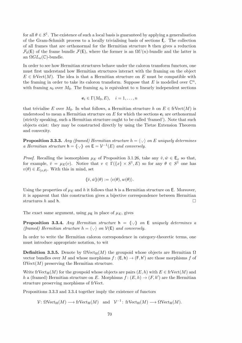
for all θ ∈ S1. The existence of such a local basis is guaranteed by applying a generalisationof the Gram-Schmidt process to a locally trivialising basis of sections fi. The collectionof all frames that are orthonormal for the Hermitian structure h then gives a reductionF0(E) of the frame bundle F(E), where the former is an ΩU(n)-bundle and the latter isan ΩGLn(C)-bundle.

In order to see how Hermitian structures behave under the caloron transform functors, onemust first understand how Hermitian structures interact with the framing on the objectE ∈ frVect(M). The idea is that a Hermitian structure on E must be compatible withthe framing in order to take its caloron transform. Suppose that E is modelled over Cn,with framing s0 over M0. The framing s0 is equivalent to n linearly independent sections

ei ∈ Γ(M0, E), i = 1, . . . , n

that trivialise E over M0. In what follows, a Hermitian structure h on E ∈ frVect(M) isunderstood to mean a Hermitian structure on E for which the sections ei are orthonormal(strictly speaking, such a Hermitian structure ought to be called ‘framed’). Note that suchobjects exist: they may be constructed directly by using the Tietze Extension Theoremand convexity.

Proposition 3.3.3. Any (framed) Hermitian structure h = 〈·,·〉 on E uniquely determinesa Hermitian structure h = 〈〈·,·〉〉 on E = V−1(E) and conversely.

Proof. Recalling the isomorphism µE of Proposition 3.1.26, take any v, w ∈ Ex so that,for example, v = µE(v). Notice that v ∈ Γ(x × S1, E) so for any θ ∈ S1 one hasv(θ) ∈ E(x,θ). With this in mind, set

〈〈v, w〉〉(θ) := 〈v(θ), w(θ)〉.

Using the properties of µE and h it follows that h is a Hermitian structure on E. Moreover,it is apparent that this construction gives a bijective correspondence between Hermitianstructures h and h.

The exact same argument, using µE in place of µE , gives

Proposition 3.3.4. Any Hermitian structure h = 〈〈·,·〉〉 on E uniquely determines a(framed) Hermitian structure h = 〈·,·〉 on V(E) and conversely.

In order to write the Hermitian caloron correspondence in category-theoretic terms, onemust introduce appropriate notation, to wit

Definition 3.3.5. Denote by ΩVectH(M) the groupoid whose objects are Hermitian Ωvector bundles over M and whose morphisms f : (E, h)→ (F, h′) are those morphisms f ofΩVect(M) preserving the Hermitian structure.

Write frVectH(M) for the groupoid whose objects are pairs (E, h) with E ∈ frVect(M) andh a (framed) Hermitian structure on E. Morphisms f : (E, h)→ (F, h′) are the Hermitianstructure preserving morphisms of frVect.

Propositions 3.3.3 and 3.3.4 together imply the existence of functors

V : ΩVectH(M) −→ frVectH(M) and V−1 : frVectH(M) −→ ΩVectH(M).

70

The action of these functors on morphisms is given by the action of the standard vectorbundle caloron transform functors, noting that Hermitian structure preserving morphismsare mapped to Hermitian structure preserving morphisms (as can be seen directly fromthe proofs of Propositions 3.3.3 and 3.3.4).

Theorem 3.3.6. The caloron correspondence for Hermitian vector bundles

V : ΩVectH(M) −→ frVectH(M) and V−1 : frVectH(M) −→ ΩVectH(M)


Proof. It suffices to notice that the natural isomorphisms βE and αE of Theorem 3.1.14preserve the Hermitian structures since βE = µ−1

E µV−1(E) and αE = µE µ−1V(E) (as in

Theorem 3.2.29).

3.3.1 Hermitian Higgs fields and module connections

A natural question to ask, given the caloron correspondences of Theorems 3.2.29 and 3.3.6,is whether there is a version of the caloron correspondence for Hermitian vector bundleswith Hermitian connections (and Higgs fields). The answer is affirmative and the result isestablished by directly combining the geometric and Hermitian caloron correspondencesfor vector bundles.

Before this correspondence is established, one first records some results relating connectivedata on Hermitian Ω vector bundles to connective data on their (unitary) frame bundles. Inparticular, one develops a notion of module connections and Higgs fields being compatiblewith a given Hermitian structure.

In the following, take (E, h) ∈ ΩVectH(M) where rankE = n so that E has structure groupΩU(n).

Definition 3.3.7. A based module connection ∆ on (E, h) is compatible with the Hermitianstructure h = 〈〈·,·〉〉 if

d〈〈v, w〉〉 = 〈〈∆(v), w〉〉+ 〈〈v,∆(w)〉〉 (3.3.8)

as LC-valued forms on M for all v, w ∈ Γ(E).

The following result is the direct analogue of Lemma 3.2.13 to the Hermitian setting:

Lemma 3.3.8. If the based module connection ∆ on E is compatible with h = 〈〈·,·〉〉 thenit uniquely determines an Ωu(n)-valued connection A on F0(E) (as in Remark 3.3.2) andconversely.

Proof. Let α be a framing of E over U , so that as usual one obtains the local (LC-module)basis ei for the fibres of E over U . Requiring α to be a section of F0(E) over U impliesthat the ei are orthonormal for h and for any v = f iei ∈ Γ(U,E)

∆(v) = f i(Aα)ji ej +mE(df i ⊗ ei),

where Aα := α∗A. If w = gj ej ∈ Γ(Uα,E), the compatibility condition (3.3.8) now readslocally as

d(f igi) = gidf i + f idgi + f igj(Aα)ji + f igj(Aα)ij

71

where the overline denotes complex conjugation as usual. Using the Leibniz rule, thisimplies

(Aα)ji + (Aα)ij = 0

and hence (Aα) ∈ Ω(U,Ωu(n)) as ∆ is based. This shows that the connection A on F0(E)is Ωu(n)-valued when restricted to orthonormal frames, so gives an ΩU(n)-connection onF0(E). The result follows from Lemma 3.2.13.

The compatibility condition for Higgs fields is

Definition 3.3.9. A Higgs field ϕ on (E, h) is compatible with the Hermitian structureh = 〈〈·,·〉〉 if

∂〈〈v, w〉〉 = 〈〈ϕ(v), w〉〉+ 〈〈v, ϕ(w)〉〉 (3.3.9)

for all v, w ∈ Γ(E), where ∂ as usual denotes differentiation in the S1 direction.

The analogue of Lemma 3.2.5 in the Hermitian setting is

Lemma 3.3.10. If the Higgs field ϕ is compatible with h = 〈〈·,·〉〉 then it uniquely deter-mines an Lu(n)-valued Higgs field Φ on F0(E) and conversely.

Proof. Let ei be trivialising orthonormal sections over U ⊂ M as in the proof of Lemma3.3.8, so that for any v = f iei ∈ Γ(U,E)

ϕ(v) = (∂f i + f jΦ(α)ij)ei.

If w = gj ej ∈ Γ(U,E), the compatibility condition (3.3.9) then reads locally as

∂(f igi) = gi∂f i + f i∂gi + f igjΦ(α)ji + f igjΦ(α)i

j .

Using the Leibniz rule for ∂ gives

Φ(α)ji + Φ(α)i

j = 0

and hence Φ(α) is Lu(n)-valued. The rest of the argument is essentially that of Lemma3.2.5.

Definition 3.3.11. Denote by ΩVectcH(M) the groupoid whose objects are quadruples(E, h,∆, φ) where (E, h) ∈ ΩVectH(M) and ∆ and φ are respectively a based moduleconnection and Higgs field on E that are compatible with h. Morphisms are given byconnection- and Higgs field-preserving morphisms of ΩVectH(M).

Similarly, write frVectcH(M) for the groupoid whose objects are triples (E, h,∇) with(E, h) ∈ frVectH(M) and ∇ a framed connection on E compatible with h. Morphisms areprecisely the connection-preserving morphisms of frVectH(M).

The geometric caloron correspondence for Hermitian vector bundles relies on the followingtwo results

Proposition 3.3.12. If the framed connection ∇ on E ∈ frVect(M) is compatible withthe Hermitian structure h = 〈·,·〉 then the module connection ∆ and Higgs field φ on(E, h) := V−1(E, h) given respectively by (3.2.6) and (3.2.7) are compatible with h = 〈〈·,·〉〉.

72

Proof. Recall (cf. Theorem 3.2.29) that ∇′ = (βE)∗∇, where

∇′ =Äpr∗M ⊗µ−1

E

ä∆ µE + dθ ⊗

Äµ−1E φ µE

äis the connection on E′ = V V−1(E). Therefore ∇′ is compatible with the inducedHermitian structure h′ = 〈βE(·), βE(·)〉 = 〈·,·〉E′ on E′.

Take any v, w ∈ Γ(E), then

d〈v, w〉E′ = 〈∇′(v), w〉E′ + 〈v,∇′(w)〉E′

where, for example, v = µE(v). Now, for all θ ∈ S1

d〈v(θ), w(θ)〉E′ = dM 〈v(θ), w(θ)〉E′ + ∂〈v(θ), w(θ)〉E′ dθ= dM 〈〈v, w〉〉(θ) + ∂〈〈v, w〉〉(θ) dθ

and

〈∇′(v)(θ), w(θ)〉E′ = 〈〈∆(v), w〉〉(θ) + 〈〈φ(v), w〉〉(θ) dθ

so that

d〈〈v, w〉〉 = 〈〈∆(v), w〉〉+ 〈〈v,∆(w)〉〉 and ∂〈〈v, w〉〉 = 〈〈φ(v), w〉〉+ 〈〈v, φ(w)〉〉

as required.

Essentially the same argument gives

Proposition 3.3.13. If the module connection ∆ and Higgs field φ on E ∈ ΩVect(M)are compatible with the Hermitian structure h = 〈〈·,·〉〉 then the framed connection ∇ on(E, h) := V(E, h) given by (3.2.5) is compatible with h = 〈·,·〉.

Combining all of these results, one arrives at the geometric caloron correspondence forHermitian vector bundles:

Theorem 3.3.14. The geometric caloron correspondence for Hermitian vector bundles

V : ΩVectcH(M) −→ frVectcH(M) and V−1 : frVectcH(M) −→ ΩVectcH(M)


Remark 3.3.15. As was observed in Remark 3.3.2, a Hermitian structure on the Ω vectorbundle E → M determines a reduction of the structure group from ΩGLn(C) to ΩU(n)(where n = rankE).

Conversely, if E comes equipped with a preferred reduction of the structure group fromΩGLn(C) to ΩU(n), then it has a Hermitian structure h = 〈〈·,·〉〉 as follows. Pick an opencover Uαα∈I of M over which E is trivialised (by maps ψα, say), so that the transitionfunctions ταβ are ΩU(n)-valued. Using the trivialisation

ψα : E|Uα −→ Uα × LCn

one may define a Hermitian structure on E|Uα that acts on elements v, w in the fibre of Eover x ∈ Uα by

〈〈v, w〉〉α(θ) :=¨ψα(v)(θ), ψα(w)(θ)

∂,

73

where 〈·,·〉 is the standard inner product on Cn. Over double intersections Uαβ := Uα∩Uβ,one has

ψβ ψ−1α : Uαβ × LCn −→ Uαβ × LCn

(x, v) 7−→ (x, ταβ(x)(v))

so that for any x ∈ Uαβ

〈〈v, w〉〉β(θ) =¨ψβ(v)(θ), ψβ(w)(θ)

∂=¨ταβ(x)(θ) · ψα(v)(θ), ταβ(x)(θ) · ψα(w)(θ)

∂=¨ψα(v)(θ), ψα(w)(θ)

∂= 〈〈v, w〉〉α(θ)

since the ταβ are ΩU(n)-valued. Therefore the 〈〈·,·〉〉α patch together to give a Hermitianstructure h = 〈〈·,·〉〉 on E that does not depend on the choice of cover Uα of M . Fromhere on, any Ω vector bundle E → M with structure group ΩU(n) is understood to beequipped with this Hermitian structure.

Example 3.3.16 (the canonical Ω vector bundles). The associated Ω vector bundle to thepath fibration PU(n) → U(n) is the canonical Hermitian Ω vector bundle of rank n,denoted E(n)→ U(n). Applying Lemmas 3.3.8 and 3.3.10 to the standard connection A∞and Higgs field Φ∞ on PU(n), one obtains the based module connection ∆(n) and Higgsfield φ(n) on E(n), noting that these are both compatible with the Hermitian structure.Since U(n) is universal for ΩU(n)-bundles, E(n) → U(n) is the universal Hermitian Ωvector bundle of rank n, however it is not necessarily universal for Hermitian Ω vectorbundles with connection; this is the reason for the disctinction in terminology betweenuniversal and canonical.

3.4 Applications to K-theory

Having given a detailed treatment of Ω vector bundles in previous sections, one is now ina position to discuss an interesting application of the theory. It turns out that Ω vectorbundles give convenient objects with which to describe odd topological K-theory. Despitebeing extravagant in dimensions, working with Ω vector bundles is advantageous since itallows one to phrase the odd K-theory of M entirely in terms of smooth bundles that arebased over M . This smoothness is critical to the construction of the Ω model in Chapter4.

3.4.1 Topological K-theory

Topological K-theory was introduced in the late 1950s by Atiyah and Hirzebruch as ageneralised cohomology theory that provides a useful tool for studying vector bundleson topological spaces. Since its first appearance (topological) K-theory has become anextremely active area of algebraic topology that has been used in the proofs of some veryfar-reaching results, notably the Atiyah-Singer Index Theorem. Some of the most well-known results of algebraic topology, such as the result of Adams giving the maximumnumber of linearly independent vector fields on the n-sphere, have relatively simple proofsusing K-theory. K-theory (and, in particular, twisted and differential K-theory) has alsofound uses in physics, where it enjoys an important role in the developing understandingof T -duality (see [7, Section 1.1] for a discussion).

74

Topological K theory is related to the notion of stable isomorphism. Over a fixed basespace X, complex vector bundles E,F → X are stably isomorphic if

E ⊕ Cn ∼= F ⊕ Cn

for some n ≥ 0. If X is compact and Hausdorff, one defines the abelian group K(X)of formal differences E − F of vector bundles over X modulo the equivalence relationE − F ∼ E′ − F ′ ⇔ E ⊕ F ′ and E′ ⊕ F are stably isomorphic4. The group operation onK(X) is given by (E − F ) + (E′ − F ′) := (E ⊕ E′) − (F ⊕ F ′), the identity element isE − E (for any choice of E) and the inverse of E − F is F − E. Alternatively, the groupK(X) may be obtained from the category Vect(X) of (topological) vector bundles over Xby applying the Grothendieck group completion device as follows.

Recall (cf. [1, Section 2.1]) that the Grothendieck construction produces from a givenabelian semi-group (A,⊕) a universal abelian group called K(A) and a homomorphismα : A → K(A) of semi-groups. The group K(A) is universal in the sense that givenany abelian group G and semi-group homomorphism β : A → G there is a unique homo-morphism γ : K(A) → G such that β = γ α. Thus, if K(A) exists it is unique up toisomorphism.

To construct K(A), first write F (A) for the free abelian group generated by elements of Aand E(A) for the subgroup of F (A) generated by those elements of the form a+a′−(a⊕a′).The K-group of A is defined to be

K(A) := F (A)/E(A)

with α : A→ K(A) the obvious map.

There is an alternative construction of K(A) that is often quite useful. Recall the diagonalmap ∆: A → A × A, which is a semi-group homomorphism, and define K(A) as thequotient semi-group

K(A) := (A×A)/∆(A).

Since (b, a) is clearly the additive inverse of (a, b), K(A) is in fact a group and one oftenwrites (a, b) as a− b so that elements of K(A) may be viewed as formal differences of ele-ments of A. The homomorphism α : A→ K(A) that characterises the universal propertyin this case is given by sending a to the coset of (a ⊕ a, a), or the coset of (a, 0) whenA has unit 0. It is readily seen from the construction that the assignment A 7→ K(A) isfunctorial.

For any compact Hausdorff space X, Vect(X)5 is a symmetric monoidal category under thedirect sum operation ⊕ on vector bundles, with identity the rank zero bundle X×0 → X.Passing to isomorphism classes6 gives the abelian semi-group (π0Vect(X),⊕) and one sets

K(X) := K(π0Vect(X)).

Since A 7→ K(A) and X 7→ π0Vect(X) are both functorial, the assignment X 7→ K(X)determines a contravariant functor from the category of compact Hausdorff topologicalspaces to the category of abelian groups. In the case that X is also a smooth manifold,

4the compactness condition on X is required to show that this equivalence relation is transitive.5the category whose objects are vector bundles over X and whose morphisms are vector bundle maps

covering the identity.6recall that for a category C, π0C denotes the isomorphism classes of C.

75

one may restrict to smooth vector bundles over X; since every topological vector bundlebased over a smooth manifold is isomorphic to a smooth vector bundle7, this gives thesame K(X).

As discussed above, elements of K(X) are virtual vector bundles over X, that is, formaldifferences E−F , where E and F are (isomorphism classes of) vector bundles over X. Therank of the virtual vector bundle E − F is simply the difference rankE − rankF , whichis constant on connected components of X. Using the Serre-Swan Theorem (cf. Remark3.4.2 or [1, Section 2.1]) every element of K(X) may be written as E −Cn for some n, sofor any E − Cn, F − Cm ∈ K(X)

E − Cn = F − Cm ⇐⇒ E ⊕ Cp ∼= F ⊕ Cq

for some p and q.

When X is a pointed space with basepoint x0, define K(X) to be the kernel of the mapı∗ : K(X)→ K(x0), where ı : x0 → X is the basepoint inclusion. If rankE = m andrankF = n, the map ı∗ sends E − F to Cm − Cn so that elements of K(X) are virtualvector bundles of rank zero on the connected component of x0 in X. Elements of K(x0)are virtual vector bundles characterised entirely by their rank, so K(x0) ∼= Z and thereis a split exact sequence

0 −→ K(X) −→ K(X) −→ Z −→ 0.

The group K(X) is referred to as the reduced K group of X.

One may extend K(X) to a cohomology theory, which in the case that X does not comeequipped with a basepoint is done in the following fashion. Write X+ := X t x0, whichis now a pointed space with basepoint x0. Then for n ∈ Z define (cf. [1, Definition 2.2.2])

Kn(X) := KÄΣ|n|(X+)

ä,

where Σ|n| denotes the |n|-th iterated reduced suspension8. Then, for example,

K0(X) = K(X) and K−1(X) = KÄ(X × S1)/(X × 0)

ä,

where Σ(X+) ∼= (X × S1)/(X × 0) is equipped with basepoint (X × 0)/(X × 0).

It is well-known that

K•(X) :=⊕n∈Z

Kn(X)

naturally has the structure of a graded ring9 and that the assignment X 7→ K•(X) deter-mines a generalised (Eilenberg-Steenrod) cohomology theory. The famous Bott PeriodicityTheorem asserts that

Kn+2(X) ∼= Kn(X)

7this can be seen, for example, by choosing a continuous classifying map into some Grassmannian andthen using [3, Proposition 17.8] to find a homotopic smooth map, as in Theorem 3.4.3.

8recall that the reduced suspension of the pointed space (Y, y0) is the space ΣY := (S1 × Y )/(S1 ∨ Y ),where S1 ∨ Y := S1 × y0 ∪ 0 × Y , equipped with the basepoint [0, y0].

9just as the group structure is induced by ⊕, the ring structure is defined using the tensor product⊗—see [1, Section 2.6] for example.

76

for any n and hence it suffices to talk only about the even and odd K-theory of X, whichare given by K0(X) and K−1(X) respectively. As topological K-theory is a 2-periodicgeneralised cohomology theory, it has a spectrum consisting of two spaces

K0(X) ∼= [X,BU × Z] and K−1(X) ∼= [X,U ]

where

U := lim−→U(n)

is the stabilised unitary group (Appendix A) and BU is its classifying space. Since spectraare determined up to homotopy equivalence, one may alternatively take BGL×Z and GLrespectively as the classifying spaces for even and odd K-theory, where

GL := lim−→GLn(C)

is the stabilised general linear group and BGL is its classifying space.

3.4.2 The functor K−1

In this section, the theory of Ω vector bundles is used to give a model for the odd K-theoryof an unpointed compact manifold M that is phrased entirely in terms of smooth objectsbased over M instead of topological vector bundles over ΣM+. In the same way that evenK-theory is given in terms of virtual vector bundles, odd K-theory is given by virtual Ωvector bundles of rank zero.

Definition 3.4.1. Let M be a compact manifold and recall that (ΩVect(M),⊕) is anabelian semi-group. Choose a basepoint x0 ∈M and define

K−1(M) := K(π0ΩVect(M)),

the abelian group obtained by using the Grothendieck group completion and then restrict-ing to the kernel of the map K(π0ΩVect(M)) → K(π0ΩVect(x0)). This definition isindependent of the choice of basepoint x0 (even if M is not connected) as the rank ofan Ω vector bundle is constant. Since the assignment M 7→ ΩVect(M) is functorial, theassignment M 7→ K−1(M) clearly determines a contravariant functor that acts on smoothmaps by pullback.

Elements of K−1(M) are virtual Ω vector bundles of rank zero, that is formal differencesE− F where E,F→M are Ω vector bundles with rankE = rankF. Strictly speaking, oneshould write [E] − [F] instead, with [E] the isomorphism class of E, however this leads toan excess of notation.

Remark 3.4.2. One observes some immediate consequences of the definition:

• Take any E− F ∈ K−1(M), then by Corollary 3.1.23 there is some Ω vector bundleG→M such that F⊕ G ∼= LCn for some n. Then

E− F = E + G− F− G = E⊕ G− LCn.

Thus every element of K−1(M) may be written in the form E−LCn where n = rankE.

77

• Suppose E− F = 0 in K−1(M). Then there is some G such that E⊕ G ∼= F⊕ G as Ωvector bundles over M . Invoking Corollary 3.1.23 again gives that there is some Hsuch that G⊕ H is trivial and hence

E⊕ G ∼= F⊕ G =⇒ E⊕ LCn ∼= F⊕ LCn

so E and F are stably isomorphic. Conversely, if E and F are stably isomorphic thenit is clear that E− F = 0 in K−1(M).

• Similarly, E−F = E′−F′ in K−1(M) if and only if E⊕F′⊕LCn ∼= E′⊕F⊕LCn for somen. In particular, E− LCn = F− LCm in K−1(M) if and only if E⊕ LCp ∼= F⊕ LCqfor some p and q.

The fact that K−1(M) gives the odd K-theory of M comes from the characterisation ofK−1(M) given above, that is

K−1(M) = KÄΣ(M+)

ä= K

Ä(M × S1)/(M × 0)

ä.

The underlying idea (glossing over smoothness requirements for now) is that a vectorbundle on (M × S1)/(M × 0) is equivalent to a vector bundle over M × S1 with adistinguished framing over M0 := M × 0 and hence, via the caloron transform, to an Ωvector bundle over M .

Consider the reduction functor

R : ΩVect(M) −→ VectÄ(M × S1)/M0

ädefined as follows. Given an Ω vector bundle E → M , its caloron transform E := V(E)is a framed vector bundle over M × S1, so has a distinguished section s0 ∈ Γ(M0,F(E)).Define an equivalence relation on E over M0 by setting

e ∼ e′ ⇐⇒ pr2 s−10 (e) = pr2 s−1

0 (e′)

recalling the notation of p. 50, with pr2 : M0×Cn → Cn the projection, and extend this toall of E by the identity. Denote by E/s0 the quotient space of E given by this equivalencerelation, then

E/s0 −→ (M × S1)/M0

is a topological vector bundle (see [1, Lemma 1.4.7], for example). The action of thereduction functor on E is given by

R(E) := V(E)/s0 ∈ VectÄ(M × S1)/M0

ä.

If f : E → F is a morphism in frVect(M) (with framings sE and sF on E and F re-spectively) it is clear from the construction that the induced map [f ] : E/sE → F/sF isan isomorphism. The action of R on morphisms is then given by sending f : E → F to[V(f)] : R(E)→ R(F).

Recall that a functor F : C→ D is essentially surjective if every object of D is isomorphicto an object in the image of F .

Theorem 3.4.3. The reduction functor

R : ΩVect(M) −→ VectÄ(M × S1)/M0

äis essentially surjective, in particular the induced map on isomorphism classes is surjective.

78

Proof. To see that R is essentially surjective, take any vector bundle E over (M ×S1)/M0

and let π : M×S1 → (M×S1)/M0 be the quotient map. Consider the pullback E′ := π∗E,which is a topological vector bundle over M × S1 with the additional property that forany two x, x′ ∈M there is an isomorphism E′(x,0) → E′(x′,0) given by

E′(x,0) 3 (x, 0, e) 7−→ (x′, 0, e) ∈ E′(x′,0).

Fix some x0 ∈M and let rankE = m, so that picking a frame p : Cm → E′(x0,0) determines

a framing r0 of E′ over M0, in particular E′|M0 is trivial. Note that E′/r0 is clearlyisomorphic to E.

Pick a classifying map f : M × S1 → Grm(Ck) for E′ so that E′ ∼= f∗γm(Ck). As bothM×S1 and Grm(Ck) are smooth manifolds, one may find a smooth map g homotopic to f[3, Proposition 17.8]. Since the pullbacks of any bundle by homotopic maps are isomorphic(see, for example, [1, Lemma 1.4.3]) E′ is isomorphic to some smooth vector bundleF := g∗γm(Ck)→M ×S1, which is trivial over M0. Pick an isomorphism f : E′ → F andconsider the framing fr0 induced on F , which is not necessarily smooth. However, fr0 ishomotopic to a smooth framing s0 of F , so since the quotient construction depends on theframing only up to homotopy [1, Lemma 1.4.7] there is an isomorphism F/s0

∼= E′/r0∼= E.

Setting F := V−1(F ), recall that V(F) and F are isomorphic as framed vector bundles andhence so too are their quotients with respect to their respective framings. In particular,R(F) is isomorphic to F/s0 and hence to E, so R is essentially surjective.

One wishes to show that R induces a bijection on isomorphism classes. It suffices to verifythat whenever R(E) and R(F) are isomorphic in Vect((M × S1)/M0) then E and F areisomorphic in ΩVect(M). Suppose that there is an isomorphism f : R(E)→ R(F), whereR(E) = E/s0 and R(F) = F/r0, say. Similarly to the proof of Theorem 3.4.3 above, onecan see that f lifts to a continuous isomorphism f ′ : E → F that respects the framings, i.e.r0 = f s0. One now requires a smooth isomorphism E → F that respects the framings,since applying the caloron transform and natural isomorphisms as necessary implies theresult.

Let m = rankE = rankF and recall from Corollary 3.1.24 that E and F are smoothlyisomorphic as framed vector bundles to some f∗γm(Ck) and g∗γm(Ck′) respectively, wherethe smooth maps f : M × S1 → Grm(Ck) and g : M × S1 → Grm(Ck′) send M0 onto therespective basepoints. Denote by f , g the maps on (M × S1)/M0 induced by f and g.

Recall, since Grm(Ck) is a quotient of GLk(C), that there are embeddings

Grm(Cm) → Grm(Cm+1) → Grm(Cm+2) → · · ·

lifting to smooth vector bundle maps

γm(Cm) → γm(Cm+1) → γm(Cm+2) → · · ·

that respect the framings. If Vectm(X) denotes the space of isomorphism classes of rankm complex vector bundles over X, recall also

Theorem 3.4.4. The map

lim−→[X,Grm(Ck)] −→ Vectm(X)

induced by pulling back the bundles γm(Ck)→ Grm(Ck) is an isomorphism for all compactHausdorff spaces X.

79

For a proof see [1, Theorem 1.4.15]. Since (M × S1)/M0 is compact and Hausdorff, thereis a homotopy h : (M × S1)/M0 × [0, 1] → Grm(CK) from f to g for some K ≥ k, k′.This implies that there is a homotopy h : M × S1 → Grm(CK) from f to g that sendsM0 × [0, 1] to the basepoint of Grm(CK). Since f and g are homotopic relative to M0,they are smoothly homotopic relative to M0 [30, Theorem 6.29].

Lemma 3.4.5. If f, g : M × S1 → Grm(Ck) are smooth maps both sending M0 to thebasepoint x0 of Grm(Ck) that are smoothly homotopic relative to M0, then there is asmooth isomorphism f∗γm(Ck) ∼= g∗γm(Ck) of framed bundles.

Proof. Take any such homotopy h : M × S1 × [0, 1] → Grm(Ck) from f to g, writinght(x, θ) = h(x, θ, t). Recall that the framing of γm(Ck) over x0 is given by taking thefirst m standard basis vectors e1, . . . , em ∈ Cm+k. By pulling back this framing by h (or,more precisely, by pulling back the corresponding trivialisation) one obtains a framing ofh∗γm(Ck) over M0 × [0, 1], namely the framing corresponding to the trivialising sectionsh∗e1, . . . , h

∗em ∈ Γ(M0 × [0, 1], h∗γm(Ck)).

Now, if ∇ is a connection on γm(Ck) then the pullback connection h∗∇ acts on the h∗eiby Ä

h∗∇äX(h∗ei) = h∗

Ä∇dh(X)ei

ä= 0

for any vector X tangent to M0 × [0, 1], as dh(X) = 0. Let ρ(x,θ) : [0, 1] → Grm(Ck) be

the smooth curve ρ(x,θ)(t) = h(x, θ, t) and let %t : h∗0γm(Ck) → h∗tγ

m(Ck) be the smoothisomorphism determined by parallel transport along the curves ρ(x,θ).

Since the tangent vector ρ(x,0)(t) to ρ(x,θ) lies tangent to M0 × [0, 1] for any t ∈ [0, 1], bythe above one has

t 7→Äh∗∇

äρ(x,0)(t)(h

∗ei) = 0

so that the sections h∗ei are parallel for the pullback connection. It follows from theuniqueness of parallel transport that the isomorphisms %t preserve the framing. Buth0 = f and h1 = g so there is a smooth isomorphism f∗γm(Ck) ∼= g∗γm(Ck) preservingthe framing.

Using this result, one at last has that f∗γm(CK) and g∗γm(CK) are smoothly isomorphicas framed vector bundles and, hence, that E and F are smoothly isomorphic as framedvector bundles. This completes the proof of

Theorem 3.4.6. The map on isomorphism classes induced by the reduction functor R isinjective and hence, by Theorem 3.4.3, is a bijection.

Notice also that if E,F are framed bundles over M × S1 with framings s0, r0 respectivelythen there is an isomorphism

E/s0 ⊕ F/r0∼= (E ⊕ F )/(s0 ⊕ r0)

and hence R(E⊕ F) ∼= R(E)⊕R(F) since V(E⊕ F) ∼= V(E)⊕ V(F).

Corollary 3.4.7. The map on isomorphism classes

π0ΩVect(M) −→ π0VectÄ(M × S1)/M0

äinduced by R is an isomorphism of semi-groups.

80

Passing to the group completions, observe that the isomorphism

K(π0ΩVect(M)) −→ KÄ(M × S1)/(M × 0)

ägiven by E− F 7→ R(E)−R(F) preserves the rank, since rankR(E) = rankE. Restrictingto the rank zero subgroups gives

Theorem 3.4.8. For any compact manifold M , the map

R : K−1(M) −→ K−1(M)

given byR : E− F 7−→ R(E)−R(F)

is an isomorphism. In particular, K−1(M) is the odd K-theory of M .

Remark 3.4.9. Another way of obtaining the isomorphism K−1 → K−1 of Theorem 3.4.8is to use the homotopy-theoretic model of odd K-theory, i.e. K−1(M) ∼= [M,GL]. Thegroup operation on K−1(M) is given by [g] + [h] := [g⊕h], with g⊕h the pointwise blocksum of g and h. At the level of homotopy, the group operations given by block sum andthe matrix product are equal so the inverse of [g] ∈ K−1(M) is the homotopy class ofthe map g−1 : x 7→ (g(x))−1 (see [40], for example). As M is compact the image of anymap f : M → GL is contained in GLn(C) for some sufficiently large n (Proposition A.4.4)and one may find a smooth map g : M → GLn(C) homotopic to f [3, Proposition 17.8].Similarly, if any two smooth maps f, g : M → GLn(C) are continuously homotopic thenthey are also smoothly homotopic [30, Theorem 6.29].

One constructs the isomorphismR : K−1(M)→ [M,GL] by sending E−LCn ∈ K−1(M) tothe homotopy class [g], where g is any classifying map (equivalently, Higgs field holonomy)for E. Observe that R is surjective, since any homotopy class [f ] ∈ [M,GL] has a smoothrepresentative g : M → GLn(C), in which case g∗E(Cn)−LCn is mapped to [f ] by R10. Tosee that R is injective, suppose that R(E− LCn) = [id] so that any classifying map for Eis homotopic to the constant map sending M to the identity in GL. Let g : M → GLn(C)be any smooth classifying map for E, then there is a smooth homotopy from g ⊕ id to idinside GLn+k(C) for some k sufficiently large. But (g ⊕ id)∗E(Cn+k) ∼= g∗E(Cn)⊕ LCk sothat g∗E(Cn) ⊕ LCk ∼= LCn+k and hence E − LCn = 0 in K−1(M). That R is a grouphomomorphism follows from the fact that g∗E(Cn)⊕ h∗E(Cm) ∼= (g ⊕ h)∗E(Cn+m).

Remark 3.4.10. By considering isomorphism classes of Hermitian structured Ω vectorbundles over M one obtains a Hermitian version of K−1(M), denoted temporarily byK−1

R (M). The argument of Remark 3.4.9 demonstrates that there is an isomorphismK−1

R (M) ∼= [M,U ], with U the stabilised unitary group. As U and GL are homo-topy equivalent this implies that the map K−1

R (M) → K−1(M) given by discarding theHermitian structure is an isomorphism and, consequently, that one may view elementsE− F ∈ K−1(M) as virtual Hermitian Ω vector bundles.

3.4.3 The total string form and the Chern character

The primary motivation for using Ω vector bundles to define odd K-theory is that theyare smooth objects that may be readily equipped with extra differential form data in the

10recalling the universal Ω vector bundles of Example 3.1.7.

81

guise of based module connections and Higgs fields. As demonstrated in Chapter 4, thisallows one to construct a differential refinement of K−1 that provides a codification of Ωvector bundles with connective data. To provide additional motivation for this discussionit is shown that the odd Chern character may be constructed on K−1 using characteristicclasses of the underlying Ω vector bundles.

Let M be a compact manifold. Recall that the Chern character is a natural map

ch : K•(M) −→ H•(M ;C)

that induces an isomorphism

ch : K•(M)⊗ C −→ H•(M ;C)

of Z2-graded rings (with the Z2-grading on H•C given by taking the even and odd degreeparts). In the case of even K-theory, the Chern character may be realised explicitly asfollows. Recall from Section 3.4.1 that an element of K0(M) is a formal difference E − Fwith E and F (isomorphism classes of) smooth complex vector bundles over M . Choosinga connection ∇ on E, write R for the curvature of ∇ and consider the even complex-valuedform

Ch(∇) := tr

Åe

12πiR

ã=∞∑j=0

1

j!

Ç1

2πi

åjtr(R ∧ · · · ∧R︸︷︷︸

j times

) (3.4.10)

on M . If E has typical fibre Cn, one can check that the degree 2k piece of Ch(∇) is exactly

cwtrk(A) = trk(F, . . . , F︸︷︷︸

k times

),

where A is the connection on the frame bundle corresponding to ∇, with curvature formF = R, and trk is the (normalised) k-th symmetrised trace, i.e. the C-valued invariantpolynomial of degree k on gln(C) given by

trk(ξ1, . . . , ξk) :=1

(k!)2(2πi)k

∑σ∈Sk

tr(ξσ(1) · · · ξσ(k)) (3.4.11)

for ξ1, . . . , ξk ∈ gln(C), with Sk the group of permutations on 1, . . . , k. It follows fromTheorem 1.1.11 that Ch(∇) is closed and the class of Ch(∇) in de Rham cohomologyis independent of ∇. Write Ch(E) ∈ Heven(M ;C) for the image of the de Rham class[Ch(∇)] under the de Rham isomorphism. It is well-known that

Ch(∇⊕∇′) = Ch(∇) + Ch(∇′) and Ch(∇⊗∇′) = Ch(∇) ∧ Ch(∇′),

so the even Chern character

ch : K0(M) −→ Heven(M ;C)

given bych : E − F 7−→ Ch(E)− Ch(F )

is a ring homomorphism.

In the case of odd K-theory, it is easier to discuss the Chern character using the homotopy-theoretic model for K−1 from the end of Section 3.4.1, i.e. K−1(M) ∼= [M,GL]. Asmentioned above, the group operation on K−1(M) is given by block sum and [g−1] is the

82

inverse of [g]. The odd Chern character of [g] ∈ K−1(M) may be computed directly bytaking a smooth representative g ∈ [g] and setting

ch([g]) =∞∑j=0

−j!(2j + 1)!

Ç− 1

2πi

åj+1

tr(g−1dg ∧ · · · ∧ g−1dg︸︷︷︸2j + 1 times

) mod exact (3.4.12)

(see [17, Proposition 1.2], for example). Since (g⊕ h)−1d(g⊕ h) = (g−1dg)⊕ (h−1dh) and(g−1)−1dg−1 = −(dg)g−1 one has

ch([g] + [h]) = ch([g ⊕ h]) = ch([g]) + ch([h]) and ch(−[g]) = ch([g−1]) = −ch([g]),

which explicitly demonstrates that the odd Chern character ch : K−1(M) → Hodd(M ;C)is a group homomorphism.

The present aim is to define the odd Chern character directly on K−1(M) using the totalstring forms (Definition 3.4.11) of the underlying Ω vector bundles. Given the Ω vectorbundle E→M equipped with based module connection ∆ and Higgs field φ, write A andΦ for the corresponding connection and Higgs field on the frame bundle F(E). Recall fromRemark 3.2.14 that if R is the curvature of ∆ and F is the curvature of A then R = F, inparticular R is Ωg-valued. Define the Higgs field covariant derivative as

∆(φ) := ∇Φ = dΦ + [A,Φ]− ∂A,

where the notation is chosen so as to indicate that ∆(φ) depends both on ∆ and on φ.

Definition 3.4.11. The total string form of the object (E,∆, φ) ∈ ΩVectc(M) is

s(∆, φ) :=∞∑j=1

1

(j − 1)!

Ç1

2πi

åj ∫S1

trÄR ∧ · · · ∧ R︸︷︷︸j − 1 times

∧∆(φ)ä,

which is an odd complex-valued form on M .

Comparing with the string forms on F(E), similarly to Ch(∇) notice that the degree 2k−1piece of s(∆, φ) is

strk(A,Φ) = k

∫S1

trk(∇Φ, F, . . . ,F︸︷︷︸k − 1 times

), (3.4.13)

with trk the k-th symmetrised trace. In particular, s(∆, φ) is closed and its cohomologyclass, which is independent of ∆ and φ, is a characteristic class for Ω vector bundles.Similarly to (3.4.10) one also has

s(∆, φ) =1

2πi

∫S1

tr

Åe

12πiR ∧∆(φ)

ã. (3.4.14)

The following result demonstrates that the total string forms are additive

Lemma 3.4.12. For any (E,∆, φ), (F,∆′, φ′) ∈ ΩVectc(M)

s(∆⊕∆′, φ⊕ φ′) = s(∆, φ) + s(∆′, φ′).

Proof. The curvature of ∆ ⊕ ∆′ is the block sum R∆ ⊕ R∆′ , with R∆, R∆′ respectivelythe curvatures of ∆ and ∆′. Similarly, the Higgs field covariant derivative of φ⊕ φ′ is theblock sum ∆(φ)⊕∆′(φ′). Since trace is additive, for every j > 0

trÄ(R∆ ⊕ R∆′)

j−1) ∧ (∆(φ)⊕∆′(φ′)ä

= trÄRj−1

∆ ∧∆(φ)ä

+ trÄRj−1

∆′ ∧∆′(φ′)ä

and the result follows.

83

For any Ω vector bundle E→M write s(E) ∈ Hodd(M ;C) for the image of the cohomologyclass [s(∆, φ)] under the de Rham isomorphism, with ∆ and φ any choice of based moduleconnection and Higgs field on E. By Lemma 3.4.12 the map

E 7−→ s(E) (3.4.15)

is a semi-group homomorphism π0ΩVect(M) → Hodd(M ;C), which extends to a grouphomomorphism

s : K−1(M) −→ Hodd(M ;C).

Explicitly, the action of s on E− F ∈ K−1(M) is

s : E− F 7−→ s(E)− s(F).

One now shows that s is indeed the odd Chern character on K−1(M), realised in terms ofΩ vector bundles.

Theorem 3.4.13. The diagram of group homomorphisms

K−1(M) K−1(M)

Hodd(M ;C)

R //

ch

s

commutes, with R the map isomorphism of Theorem 3.4.8. In particular,

s : K−1(M) −→ Hodd(M ;C)

is the odd Chern character.

Proof. In the homotopy-theoretic model for K−1, the isomorphism R is given by

E− F 7−→ [g]⊕ [h]−1 = [g ⊕ h−1]

where g, h : M → GLn(C) are smooth classifying maps for E and F respectively for somesufficiently large n (see Remark 3.4.9).

Choose based module connections ∆, ∆′ and Higgs fields φ, φ′ on E and F respectively.By Lemma 3.2.6 one may take g = holφ and h = holφ′ , in which case by Lemma 1.2.8 andTheorem 1.2.11 one has, for example,

s(∆, φ) =∞∑j=1

g∗τ (trj) =∞∑j=1

Å−1

2

ãj−1 j!(j − 1)!

(2j − 1)!g∗ trj

ÄΘ, [Θ,Θ]j−1

ä+ exact,

with Θ the Maurer-Cartan form on GLn(C). Now,

trjÄΘ, [Θ,Θ]j−1

ä=

2j−1

j!(2πi)jtr(Θ2j−1),

and g∗Θ = g−1dg, so that

s(∆, φ) =∞∑j=1

−(j − 1)!

(2j − 1)!

Å− 1

2πi

ãjtrÄ(g−1dg)2j−1

ä+ exact.

84

Shifting the degree of the sum, by the additivity of trace

s(E− F) =∞∑j=0

−j!(2j + 1)!

Å− 1

2πi

ãj+1

tr

Å[Äg ⊕ h−1

ä−1dÄg ⊕ h−1

ä]2j+1ã

+ exact.

Comparing this with the expression (3.4.12) for the odd Chern character gives

s(E− F) = ch([g ⊕ h−1]) = ch(R(E− F))

as required.

If Θ now denotes the Maurer-Cartan form on GL (see Appendix A), set

τGL :=∞∑j=0

−j!(2j + 1)!

Å− 1

2πi

ãj+1

trÄΘ2j+1

ä(3.4.16)

and define the space of closed odd degree complex-valued forms

∧GL (M) := g∗τGL | g : M −→ GL is smooth. (3.4.17)

Under the pointwise block sum and matrix inversion operations on the space of smoothmaps M → GL one has

(g ⊕ h)∗τGL = g∗τGL + h∗τGL and (g−1)∗τGL = −g∗τGL

so that ∧GL(M) is a subgroup of Ωodd(M ;C). The proof of Theorem 3.4.13 gives

Corollary 3.4.14. If s : K−1(M)→ HodddeR(M ;C) is the odd Chern character on K−1(M)

valued in complex de Rham cohomology, then im s = ∧GL(M) mod exact and so ∧GL(M)generates the odd complex de Rham cohomology of M .

In light of Remark 3.4.10, there is also a Hermitian version of the odd Chern characterthat maps K−1(M) into real-valued singular cohomology. It is given by sending the vir-tual Hermitian Ω vector bundle E − F to the cohomology class of the closed real-valueddifferential form s(∆, φ) − s(∆′, φ′), where ∆ and ∆′, φ and φ′ are any choice of basedmodule connections and Higgs fields on E and F respectively that are compatible with theHermitian structure. The reason that s(∆, φ), for example, is a real-valued form is that

s(∆, φ) =

∫S1Ch(∇)

where ∇ is the caloron-transformed connection: since ∇ is compatible with the caloron-transformed Hermitian structure, if R denotes its curvature then the form 1

iR takes valuesin Hermitian matrices so Ch(∇) is a real-valued form.

One may prove a Hermitian version of Theorem 3.4.13 following the same argument asabove, and setting

τ :=∞∑j=0

−j!(2j + 1)!

Å− 1

2πi

ãj+1

trÄΘ2j+1

ä(3.4.18)

with Θ the Maurer-Cartan form on U , one defines the space of closed odd degree real-valued forms

∧U (M) := g∗τ | g : M −→ U is smooth. (3.4.19)

Similarly to ∧GL(M), ∧U (M) has an abelian group structure induced by the block sumoperation on smooth maps M → U . One also has

85

Corollary 3.4.15. If s : K−1(M) → HodddeR(M) is the odd Chern character on K−1(M)

valued in de Rham cohomology, then im s = ∧U (M) mod exact and so ∧U (M) generatesthe odd de Rham cohomology of M .

86

Chapter 4

The Ω model for odd differentialK-theory

In this chapter, the theory of Ω vector bundles developed in Chapter 3 is used to constructa differential extension of odd topological K-theory—the Ω model—which is shown to bea model for odd differential K-theory.

A differential extension E of the generalised (Eilenberg-Steenrod) cohomology theory Eis a geometric refinement of E that naturally includes additional differential form data.When the underlying cohomology theory E is multiplicative, the differential extension E ismultiplicative if it has a graded ring structure that respects the cohomological and differen-tial form data. In their seminal paper [26], Hopkins and Singer demonstrated that everygeneralised cohomology theory has a differential extension. Following this, Bunke andSchick [5, 6, 7] provided an axiomatic characterisation of differential extensions togetherwith a result, under certain mild conditions on the underlying cohomology theory, thatguarantees the uniqueness of multiplicative differential extensions up to unique isomor-phism (these axioms and uniqueness results are recorded in Appendix C). In point of fact,this unique isomorphism can be constructed without a multiplciative structure providedthat the differential extension has a special pushforward map called an S1-integration. Inparticular, since K-theory satisfies the requisite conditions, any two differential extensionsof K-theory with S1-integration are isomorphic via a unique isomorphism: this is what ismeant by differential K-theory.

Differential K-theory has been studied extensively in recent years. Consequently, there area variety of different constructions of differential K-theory; for a detailed survey see [7].As with ordinary K-theory, the additive structure of differential K-theory splits into evenand odd degree parts resulting in even and odd differential K-theory. The Bunke-Schickuniqueness results are sufficient to guarantee that any two differential extensions of theeven part of K-theory are uniquely isomorphic, even without a multiplicative structure oran S1-integration. Consequently, any differential extension of the even part of K-theorydefines even differential K-theory. However, this is not true for odd K-theory and in factone can show that there are infinitely many non-isomorphic differential extensions of oddK-theory [6].

It is particularly important to have accessible geometric models for differential extensions,not least because this is the most common way that differential extensions appear inphysics. In gauge theory, for example, gauge fields are described by ordinary differential

87

cohomology and it is suggested by Freed [13] that differential K-theory (or rather, twisteddifferential K-theory) describes Ramond-Ramond fields in type II string theory.

In [38], Simons and Sullivan construct a simple geometric model for the even degree partof differential K-theory using vector bundles with connection. The principle behind thisconstruction is that, insofar as even K-theory is related to stable isomorphism classesof vector bundles, even differential K-theory is related to stable isomorphism classes ofvector bundles with connection, where the stability condition is extended to connectivedata using the Chern-Simons forms. This model of even differential K-theory provides astraightforward codification of vector bundles with connection.

In this chapter, an analogous geometric model for odd differential K-theory is constructedby using Ω vector bundles and their associated geometric data in place of vector bundles:this is the Ω model for odd differential K-theory. Motivated by the results of Section3.4.2, where it was shown that virtual Ω vector bundles of rank zero give odd K-theory,one shows that the odd part of differential K-theory may be obtained in a similar fashionby using Ω vector bundles equipped with based module connections and Higgs fields. Thestring potentials of Chapter 2 play a central role in the construction of the Ω model, whichgives a straightforward geometric model for odd differential K-theory complementing thework of Simons and Sullivan.

To aid the discussion, an explicit isomorphism is constructed between the Ω model and anelementary differential extension of odd K-theory described recently by Tradler, Wilsonand Zeinalian [40]. This isomorphism provides a homotopy-theoretic interpretation of theΩ model as well as a proof that the TWZ extension does indeed define odd differentialK-theory, this latter result being speculated but not proved in [40].

Throughout this chapter, unless stated otherwise M shall always be taken to be a compactfinite-dimensional manifold, possibly with corners, and all Ω vector bundles are taken tobe Hermitian.

4.1 Structured vector bundles

The primary ingredient in the construction of the Ω model is the notion of structured Ωvector bundles. These are Ω vector bundles equipped with a certain equivalence class ofbased module connections and Higgs fields.

4.1.1 The Simons-Sullivan model

The construction of the Ω model is motivated by the Simons-Sullivan model1 for evendifferential K-theory developed in [38]. Consider a complex, finite-rank Hermitian vectorbundle E →M with compatible connection ∇. Recall that the Chern character of E maybe represented by the real-valued closed form

Ch(∇) =∞∑j=0

1

j!

Ç1

2πi

åjtr(R ∧ · · · ∧R︸︷︷︸

j times

),

1in this thesis, one considers only the Hermitian version of the Simons-Sullivan construction—there isalso a version that does not use Hermitian structures.

88

with R the curvature of ∇. If γ : t 7→ ∇t is a smooth path of connections2 on E with Btthe time derivative of the path γ, the Chern-Simons form of γ is

CS(γ) :=∞∑j=1

1

(j − 1)!

Ç1

2πi

åj ∫ 1

0tr(Bt ∧Rt ∧ · · · ∧Rt︸︷︷︸

j − 1 times

) dt,

with Rt the curvature of ∇t. It is well-known that dCS(γ) = Ch(∇1)− Ch(∇0).

Since spaces of connections are affine, there is always a smooth path between any pair ofconnections on E. If there is a path γ from ∇0 to ∇1 such that CS(γ) is exact then itturns out that CS(ν) is exact for any smooth path ν from ∇0 to ∇1 [38, Proposition 1.1]and, in particular, Ch(∇0) = Ch(∇1). Setting

CS(∇0;∇1) := CS(γ) mod exact

for any smooth path γ from ∇0 to ∇1, one defines an equivalence relation on the space ofconnections on E by setting ∇0 ∼ ∇1 ⇔ CS(∇0;∇1) = 0 mod exact.

Definition 4.1.1 ([38]). A structured vector bundle over M is a pair E = (E, [∇]) withE →M a Hermitian vector bundle and ∇ an equivalence class of compatible connectionson E.

Example 4.1.2 (The trivial structured bundle of rank n). The trivial structured bundle ofrank n over M is n = (Cn, [d]), with Cn = M × Cn → M the trivial bundle of rank n(with its canonical Hermitian structure) and d the trivial connection.

The equivalence relation on connections described above behaves well with respect topullbacks. In particular, one may pull back structured vector bundles by smooth mapsand there is a natural notion of isomorphism for structured vector bundles. The directsum and tensor product operations on vector bundles with connection also give rise towell-defined operations ⊕ and ⊗ on structured vector bundles; for details the interestedreader is referred to [38].

Definition 4.1.3 ([38]). Define Struct(M) to be the set of all isomorphism classes ofstructured vector bundles over M , which is a commutative semi-ring under the operations⊕ and ⊗. To avoid excessive notation, elements of Struct(M) are denoted E rather than[E]. The assignment

M 7−→ Struct(M)

determines a contravariant functor

Struct : Man −→ SemiRing

from the category of smooth compact manifolds with corners to the category of semi-rings.

The following special types of structured bundles are important for understanding howstructured vector bundles give rise to even differential K-theory.

Definition 4.1.4 ([38]). A structured vector bundle E = (E, [∇]) is stably trivial if thereis some k such that E⊕ Ck ∼= Cn+k. Write

StructT (M) := E ∈ Struct(M) | E is stably trivial2defined similarly to Definition 2.1.3.

89

for the semi-group of those isomorphism classes in Struct(M) containing a stably trivialstructured vector bundle.

A structured vector bundle E is stably flat if E ⊕ k = n + k for some k. Write

StructF (M) := E ∈ Struct(M) | E is stably flat

for the semi-group of those isomorphism classes in Struct(M) containing a stably flatstructured vector bundle. Clearly StructF (M) ⊂ StructT (M) and is a sub-semi-group.

The Grothendieck group completion applied to Struct(M) gives the commutative ring

K0(M) := KÄ

Struct(M)ä, (4.1.1)

where, as usual, elements of K0(M) are denoted as formal differences E − F . Everystructured bundle E has an inverse, i.e. a structured bundle F such that E ⊕ F ∼= n forsome n, so one may write any element of K0(M) in the form E − n [38, Theorem 1.8].One may also show that E − n = 0 ∈ K0(M) if and only if E is stably flat.

There is a natural transformation of functors

Ch : Struct(M) −→ Ωevend=0 (M)

given by Ch : E = (E, [∇]) 7→ Ch(∇). In fact, Ch is a semi-ring homomorphism, that is

Ch(E ⊕ F ) = Ch(E) + Ch(F ) and Ch(E ⊗ F ) = Ch(E) ∧ Ch(F )

[38, (1.11)]. Passing to K0(M) gives the ring homomorphism

Ch : E − F 7−→ Ch(E)− Ch(F ).

Write δ : K0(M) → K0(M) for the obvious forgetful map that discards the connectivedata, i.e. E − F 7→ E − F . Recalling that K0(M) may be defined entirely in terms ofsmooth vector bundles, it follows that δ is surjective. The maps δ and Ch fit into thecommuting diagram of ring homomorphisms

K0(M) K0(M)

Ωevend=0 (M) Hodd(M ;R)

δ //

deR //

Ch

ch

with deR the natural map given by the de Rham isomorphism and ch the even Cherncharacter. This gives part of the data required for a differential extension of the even partof K-theory: Ch is the curvature morphism and δ is the underlying class morphism ofK0(M).

The final datum that makes K0(M) a differential extension of K0(M) is the action offorms morphism a : Ωodd(M)/im d → K0(M), along with the associated exact sequence.It is useful for the constructions in the sequel to examine how this map works in somedetail.

90

Say that a connection ∇ on E is Flat if it has trivial holonomy around every closed curve[38, Definition 1.7]. This implies that the curvature of ∇ vanishes and (by finding parallelsections for ∇) that E is isomorphic to the trivial bundle Cn with the trivial connection.Recall from (3.4.19) the space of odd forms ∧U (M), then

Lemma 4.1.5 ([38]). For any pair of Flat connections ∇, ∇′ on E that are compatiblewith the Hermitian structure

CS(∇;∇′) ∈ ∧U (M) mod exact.

Digressing for the moment, one also has

Lemma 4.1.6. Let d be a Flat connection on the Hermitian vector bundle E → M andg : M → U(n) a smooth map, with n = rankE. Then there is a Flat connection d on Eand a smooth path γ of connections compatible with the Hermitian structure from d to dsuch that

CS(γ) = g∗τ,

with τ the form of (3.4.18).

Proof. Compare with the proof of [38, Lemma 2.1]. By taking a global framing of E thatis parallel for d, one may suppose that E = Cn with its standard Hermitian structure andthat d is the trivial product connection. Then, if Θ is the Maurer-Cartan form on U(n)define the Flat compatible connection d := d+ g∗Θ = d+ g−1dg.

Define a smooth path of connections by γ(t) := ∇t = d+ tg∗Θ noting that the curvatureof ∇t is given by td(g∗Θ) + t2g∗Θ ∧ g∗Θ = (t2 − t)g∗(Θ ∧Θ) since dΘ = −Θ ∧Θ. Then

CS(γ) =∞∑j=1

1

(j − 1)!

Ç1

2πi

åj ∫ 1

0(t2 − t)j−1 dt · tr

Ä(g∗Θ)2j−1

ä=∞∑j=0

−j!(2j + 1)!

Å− 1

2πi

ãj+1

trÄ(g∗Θ)2j+1

ä= g∗τ,

which is the desired result.

Given any stably trivial E ∈ StructT (M), take trivial Hermitian vector bundles F and Hsuch that E ⊕ F ∼= H and set

CS(E) := CS(∇H ;∇⊕∇F ) mod ∧U (M)

for any choice of Flat connections ∇H on H and ∇F on F compatible with the Hermitianstructure, noting that this is independent of choices by Lemma 4.1.5. This defines asemi-group homomorphism [38, Proposition 2.3]

CS : StructT (M) −→ Ωodd(M)/∧U (M),

where ∧U (M) := ∧U (M) + dΩeven(M).

Theorem 4.1.7 ([38]). CS is surjective with kernel StructF (M). Therefore

CS : StructT (M)/ StructF (M) −→ Ωodd(M)/∧U (M)

is a semi-group isomorphism, which implies that StructT (M)/ StructF (M) is a group.

91

By postcomposing CS−1

with the isomorphism

Γ: StructT (M)/ StructF (M) −→ ker δ (4.1.2)

that sends E 7→ E − n, with n = rankE, one obtains the exact sequence

0 −→ Ωodd(M)/∧U (M)ı−−→ K0(M)

δ−−→ K0(M) −→ 0

where ı = Γ CS−1

. One defines the action of forms morphism a as the composition

Ωodd(M)/im d −→ Ωodd(M)/ ∧U (M)ı−−→ K0(M), (4.1.3)

where the first map is the natural projection given by the identification

Ωeven(M)/ ∧U (M) =ÄΩeven(M)/im d

ä/∧U (M).

Corollary 3.4.15 demonstrates that ∧U (M) mod exact is the image of the odd Cherncharacter, so the sequence

K−1(M)ch−−−→ Ωodd(M)/im d

a−−→ K0(M)δ−−→ K0(M) −→ 0

is exact. One may also show that Ch a = d [38, Proposition 3.2] so that K0 is indeed adifferential extension of even K-theory. By the Bunke-Schick uniqueness result (TheoremC.2.2) it follows that K0 is naturally isomorphic to the even part of any other differentialextension of K-theory via a unique isomorphism. The Simons-Sullivan model for evendifferential K-theory has a definite geometric appeal since it provides a clear codificationof vector bundles with connection. Moreover, the construction of this model involves lessgeometric data than other models; compare with the Freed-Lott model [15], which requiresan additional differential form.

Remark 4.1.8. As a concluding remark to round off this section, one makes an observationthat is required in the sequel. Given any ω ∈ Ωodd(M), by definition a(ω) := E − nwhere E = (E, [∇]) ∈ Struct(M) is such that

• rankE = n and E is trivial; and

• for any chosen representative ∇ ∈ [∇] there is a smooth path γ′ of connections fromsome Flat connection d to ∇ such that the Chern-Simons form

CS(γ′) = ω mod ∧U (M),

i.e. CS(γ′) = ω+g∗τ +dχ for some smooth g : M → U . Invoking Lemma 4.1.6, afterpossibly stabilising by a trivial bundle with its trivial connection, this implies thatthere is a path of connections γ from some Flat connection d to ∇ such that

CS(γ) = ω mod exact.

4.1.2 Structured Ω vector bundles

The construction of the Ω model proceeds by analogy with the Simons-Sullivan model;accordingly the first notion required is that of structured Ω vector bundles.

92

Take the Hermitian Ω vector bundle (E, h) over M (of rank n, say) equipped with basedmodule connection ∆ and Higgs field φ that are compatible with h. From this pointonward, it shall be standard to omit explicit reference to the Hermitian structure h andrefer to E simply as a Hermitian vector bundle, with a choice of h assumed. Write R forthe curvature of ∆ and ∆(φ) for the Higgs field covariant derivative of φ, recalling thetotal string form

s(∆, φ) =∞∑j=1

1

(j − 1)!

Ç1

2πi

åj ∫S1

tr(R ∧ · · · ∧ R︸︷︷︸j − 1 times

∧∆(φ)),

which is the odd Chern character on K−1. Just as the string forms play the role of theChern character on K−1, the relative string potentials play the part of relative Chern-Simons forms in the Ω model.

To see how this works, as in Section 2.1 define a smooth n-cube of based module connectionson E as a based module connection ∆ on the Ω vector bundle E × [0, 1]n → M × [0, 1]n

such that ∆Xs = 0 for any vector field X on M × [0, 1]n that is vertical for the projectionM × [0, 1]n → M and section s pulled back to M × [0, 1]n from M . A smooth n-cube ofHiggs fields on E is a Higgs field φ on E× [0, 1]n and since E is Hermitian, smooth n-cubesof connections and Higgs fields are required to be compatible with the Hermitian structureinduced on E× [0, 1]n.

Recalling the notation of Definitions 3.2.1 and 3.2.16, let HE and ME respectively be thespaces of Higgs fields and based module connections on E that are compatible with theHermitian structure. A smooth map

γ : [0, 1]n −→ME ×HE

is an assignment

γ : (t1, . . . , tn) 7−→Ä∆(t1,...,tn), φ(t1,...,tn)

äwith

∆(t1,...,tn) = ς∗(t1,...,tn)∆γ and φ(t1,...,tn) = ς∗(t1,...,tn)φ

γ

for some smooth n-cubes of based module connections ∆γ and Higgs fields φγ on E. Asin the principal bundle case, specifying such a smooth map γ is equivalent to specifyingsmooth n-cubes ∆γ and φγ . A straightforward argument using the proofs of Lemmas 3.2.5and 3.2.13 demonstrates that smooth maps

[0, 1]n −→ME ×HE and [0, 1]n −→ AF(E) ×HF(E)

are in bijective correspondence, with F(E) the unitary frame bundle of E determined bythe Hermitian structure.

Take a smooth path γ : [0, 1]→ME×HE, writing Fγ for the corresponding smooth path[0, 1]→ AF(E) ×HF(E).

Definition 4.1.9. For j > 0, the j-th string potential of the path γ is the (2j − 2)-form

Sj(γ) := j

∫ 1

0

∫S1

((j − 1)trj

ÄBt,Rt, . . . ,Rt︸︷︷︸

j−2 times

,∆t(φ)ä

+ trjÄRt, . . . ,Rt︸︷︷︸j−1 times

, ϕtä)dt

93

where Rt is the curvature of ∆t, ∆t(φ) is the Higgs field covariant derivative of φt (withrespect to ∆t) and

Bt := ς∗t (L∂t∆γ) and ϕt := ς∗t (L∂tφγ)

are the time derivatives of ∆t and φt along the path, which are both Ωu(n)-valued forms.The invariant polynomials trk on u(n) are the symmetrised traces of (3.4.11).

The total string potential of γ is the form

S(γ) =∞∑j=1

Sj(γ),

whose degree 2k − 2 piece is the k-th string potential. The forms Sj(γ) and S(γ) appearto live on the total space E but are in fact basic by Theorem 4.1.10 below.

If Fγ(t) := (At,Φt) is the smooth path of connections and Higgs fields on the frame bundleF(E) corresponding to γ then Rt = Ft and ∆t(φ) = ∇Φt, where Ft is the curvature of theconnection At. The arguments of Lemmas 3.2.5 and 3.2.13 also show that

ς∗tÄL∂tAF(γ)

ä= ς∗t (L∂t∆γ) and ς∗t

ÄL∂tΦF(γ)

ä= ς∗t (L∂tΦγ)

and hence the j-th string potential satisfies

Sj(γ) = Strj(F(γ)), (4.1.4)

where the right hand side is a relative string potential form as in Chapter 2.

Theorem 4.1.10. For any smooth path γ : [0, 1] → ME × HE, the j-th and total stringpotentials descend to M and the total string potential satisfies

dS(γ) = s(∆1, φ1)− s(∆0, φ0).

Proof. Applying Theorem 2.1.8 to the j-th string potential shows that Sj(γ) is basic and

dSj(γ) = dStrj(F(γ)) = strj

(A1,Φ1)− strj(A0,Φ0),

which is precisely the degree 2j − 1 piece of s(∆1, φ1)− s(∆0, φ0).

Similarly to the expression (2.1.4) relating the (principal bundle) string potentials andstring forms, by (3.4.13) and (4.1.4) one has

S(γ) =

∫ 1

0ς∗t ı∂ts(∆

γ , φγ) dt. (4.1.5)

Another result that transfers over readily from the principal bundle case is

Proposition 4.1.11. If γ0, γ1 : [0, 1]→ME×HE are smooth paths with the same endpointsthen S(γ1)− S(γ0) is exact.

Due to this last result, one may use the string potentials to define an equivalence relationthat is analogous to Chern-Simons exactness. For any two pairs (∆0, φ0) and (∆1, φ1)of based module connections and Higgs fields on E compatible with the given Hermitianstructure, there is a smooth path γ from (∆0, φ0) to (∆1, φ1). Set

S(∆0, φ0; ∆1, φ1) := S(γ) mod exact (4.1.6)

94

for any such path, which is well-defined by Proposition 4.1.11. Moreover,

S(∆0, φ0; ∆2, φ2) = S(∆0, φ0; ∆1, φ1) + S(∆1, φ1; ∆2, φ2)

and since S(γ) = 0 for a constant path one has S(∆0, φ0; ∆1, φ1) = −S(∆1, φ1; ∆0, φ0).

Define pairs (∆0, φ0) and (∆1, φ1) as above to be equivalent, denoted (∆0, φ0) ∼ (∆1, φ1)if and only if

S(∆0, φ0; ∆1, φ1) = 0 mod exact.

This is an equivalence relation and an equivalence class [∆, φ] is a string datum on E. Bydirect analogy with structured vector bundles

Definition 4.1.12. A structured Ω vector bundle over M is a pair E = (E, [∆, φ]), withE → M a Hermitian Ω vector bundle and [∆, φ] a string datum on E. The rank of thestructured Ω vector bundle E is rankE := rankE.

Example 4.1.13. The trivial structured Ω vector bundle over M of rank k is

LCk =ÄLCk, [δ, ∂]

äwhere δ is the trivial module connection and ∂ is the trivial Higgs field on the trivial Ωvector bundle LCk over M equipped with its canonical Hermitian structure.

An important type of structured Ω vector bundle is

Example 4.1.14. The canonical structured Ω vector bundle of rank n is

E(n) :=ÄE(n), [∆(n), φ(n)]

ä,

where E(n)→ U(n) is the canonical Hermitian Ω vector bundle of rank n with its standardgeometric data ∆(n), φ(n)—see Example 3.3.16.

Given a structured Ω vector bundle E = (E, [∆, φ]) over M and a smooth map f : N →M ,one may define the pullback f∗E as (f∗E, [f∗∆, f∗φ]). This is well-defined since the stringforms and string potentials are natural so that

f∗S(∆0, φ0; ∆1, φ1) = S(f∗∆0, f∗φ0; f∗∆1, f

∗φ1).

Structured Ω vector bundles E = (E, [∆, φ]) and F = (F, [∆′, φ′]) are isomorphic if there isan isomorphism f : F→ E of Ω vector bundles such that [∆′, φ′] = f∗[∆, φ] := [f∗∆, f∗φ].

In this thesis it is important to know how structured Ω vector bundles behave undersmooth homotopy. Suppose that ft : N → M is a family of smooth maps dependingsmoothly on the parameter t ∈ [0, 1], equivalently a smooth map F : N× [0, 1]→M whereF (·, t) = ft. Take a Hermitian Ω vector bundle E → M with compatible based moduleconnection ∆ and Higgs field φ and for t ∈ [0, 1] consider the pullbacks f∗t (E), which areHermitian Ω vector bundles with compatible connections f∗t ∆ and Higgs fields f∗t φ.

Let E be the caloron transform of E equipped with the Hermitian caloron-transformedconnection ∇. Define the family of smooth curves ρx : [0, 1] → M by ρx(t) := ft(x) forx ∈ N . Similarly to [38, p. 584] and Lemma 3.4.5, let %t : (f0 × id)∗E → (ft × id)∗Ebe the smooth isomorphisms determined by parallel transport along the family of curvesρx,θ(t) := (ft(x), θ), observing that the %t cover the identity on N × S1.

95

Set F := (f0 × id)∗E and ∇t := %∗t (f0 × id)∗∇, noting that for all t ∈ [0, 1] the connection∇t is compatible with the induced Hermitian structure on F . Write ρx,θ(t) for the tangentvector to ρx,θ at t, then

CS(∇0,∇1) =

∫ 1

0(ft × id)∗ıρx,θ(t)Ch(∇) dt mod exact

(cf. [38, (1.8)]). Recall that

s(∆, φ) =

∫S1Ch(∇),

then by Lemma B.1.3 and the fact that ρx,θ(t) has no S1-component,∫S1

(ft × id)∗ = f∗t

∫S1

and

∫S1ıρx,θ(t) = ıρx(t)

∫S1

so after integrating over the fibre one obtains

S(∆0, φ0; ∆1, φ1) =

∫ 1

0f∗t ıρx(t)s(∆, φ) dt mod exact, (4.1.7)

where ∆t, φt correspond to the connection ∇t. This argument shows that f∗t E∼= f∗0E for

any t ∈ [0, 1] and also that

S(f∗0 ∆, f∗0φ; f∗1 ∆, f∗1φ) =

∫ 1

0f∗t ıρx(t)s(∆, φ) dt mod exact, (4.1.8)

abusing notation slightly by omitting the isomorphism f∗1E∼= f∗0E.

The direct sum operation ⊕ on ΩVect(M) extends to structured Ω vector bundles

Lemma 4.1.15. Let E,F be Ω vector bundles over M and take any pair of smooth pathsγ : [0, 1]→ME ×HE and σ : [0, 1]→MF ×HF. These together determine a smooth path

γ ⊕ σ : [0, 1]→ME⊕F ×HE⊕F

via γ ⊕ σ(t) := (∆γt ⊕∆σ

t , φγt ⊕ φσt ). Then

S(γ ⊕ φ) = S(γ) + S(φ)

and by Theorem 4.1.10

dS(γ ⊕ φ) = s(∆γ1 ⊕∆σ

1 , φγ1 ⊕ φ

σ1 )− s(∆γ

0 ⊕∆σ0 , φ

γ0 ⊕ φ

σ0 ).

Moreover, for any choice of pairs (∆, φ), (∆, φ) on E and (∆′, φ′), (∆′, φ′) on F

S(∆⊕∆′, φ⊕ φ′; ∆⊕ ∆′, φ⊕ φ′) = S(∆, φ; ∆, φ) + S(∆′, φ′; ∆′, φ′)

Proof. Compare with [38, Lemma 1.4]. The proof of the first two assertions is essentiallythat of Lemma 3.4.12, since the curvatures and time derivatives are block sums.

The last assertion follows from

S(∆⊕∆′, φ⊕ φ′; ∆⊕ ∆′, φ⊕ φ′) = S(∆⊕∆′, φ⊕ φ′; ∆⊕ ∆′, φ⊕ φ′)+ S(∆⊕ ∆′, φ⊕ φ′; ∆⊕ ∆′, φ⊕ φ′)

and by using the first assertion, i.e.

S(∆⊕∆′, φ⊕ φ′; ∆⊕ ∆′, φ⊕ φ′) = S(∆′, φ′; ∆′, φ′)

and similarly for the second term.

96

It follows immediately that the direct sum operation is well-defined on string data, so ifE = (E, [∆, φ]) and F = (F, [∆′, φ′]) are structured Ω bundles over M then their direct sum

E⊕ F :=(E⊕ F,

[∆⊕∆′, φ⊕ φ′

])is a structured Ω bundle over M . Note there is an obvious isomorphism E⊕ F ∼= F⊕ E.

In order to define the Ω model, it is necessary to consider a special class of structuredHermitian Ω vector bundles, namely those structured Ω vector bundles that are pullbacksof E(n) for some n (Example 4.1.14). Observe that if g : M → U(n) and h : M → U(m)are smooth maps then the block sum

g ⊕ h : x 7−→Çg(x) 0

0 h(x)

åis a smooth map g ⊕ h : M → U(n + m) and there is an isomorphism of structured Ωvector bundles

g∗E(n)⊕ h∗E(m)∼−−→ (g ⊕ h)∗E(n+m).

The trivial structured Ω vector bundle LCn coincides with the pullback of E(n) by aconstant map M → U(n).

Definition 4.1.16. Define StructΩ(M) to be the set of isomorphism classes of structuredΩ vector bundles

StructΩ(M) := [g∗E(n)] | g is a smooth map M → U(n) for some n.

Since h∗E(m) ⊕ g∗E(n) ∼= g∗E(n) ⊕ h∗E(m) ∼= (g ⊕ h)∗E(n + m) for any smooth mapsg : M → U(n), h : M → U(m), StructΩ(M) is an abelian semi-group under the directsum operation on structured Ω vector bundles. A smooth map f : N → M induces thepullback map f∗ : StructΩ(M)→ StructΩ(N) respecting the semi-group structure, so thatthe assignment

M 7−→ StructΩ(M)

determines a contravariant functor from the category of smooth compact manifolds withcorners to the category of abelian semi-groups.

Remark 4.1.17. StructΩ(M) is a special set of isomorphism classes of structured Ω vectorbundles. The primary reason for making this restriction is Theorem 4.1.18 below, whichguarantees that every element E of StructΩ(M) has an ‘inverse’, i.e. that there is someF ∈ StructΩ(M) such that E ⊕ F is trivial. One expects that any arbitrary structured Ωvector bundle E over M (not necessarily isomorphic to a pullback of some E(n)) shouldhave an inverse, however a proof of this fact has not yet been found.

From Theorem 4.1.10 and the definition of string data the map

s : StructΩ(M) −→ Ωoddd=0(M) (4.1.9)

given by(E, [∆, φ]) 7−→ s(∆, φ)

is a well-defined semi-group homomorphism. It is shown below in Section 4.2 that afterpassing to the group completion, this is the curvature morphism of the Ω model.

The following theorem is crucial to the construction of the Ω model and the proof is basedon related work appearing in [38, 40].

97

Theorem 4.1.18. Let g : M → U(n) be any smooth map. Then there is an isomorphismof structured Ω vector bundles

g∗E(n)⊕ (g−1)∗E(n) ∼= LC2n.

Proof. As remarked above, the structured Ω vector g∗E(n) ⊕ (g−1)∗E(n) coincides withthe pullback of E(2n) by the block sum map

g ⊕ g−1 : x 7−→Çg(x) 0

0 g(x)−1

å∈ U(2n)

and the structured Ω vector bundle LC2n is the pullback of E(2n) by the constant mapat the identity. The method of this proof is to construct a certain smooth homotopy fromg ⊕ g−1 to id and then use (4.1.8).

Similarly to [40, Lemma 3.6], define the smooth map R : [0, π2 ]→ U(2n) by setting

R(t) :=

Çcos t − sin tsin t cos t

åwhich is a block matrix consisting of n× n blocks. Writing

A =

Çg 00 1

åand B =

Ç1 00 g−1

å,

for t ∈ [0, π2 ] consider the map Xt : M → U(2n) given by

Xt := AR(t)BR(t)−1.

The assignment M × [0, π2 ] → U(2n) sending (x, t) 7→ Xt(x) is a smooth homotopy fromg ⊕ g−1 to the identity and by direct calculation

X−1t ∂tXt = R(t)B−1JBR(t)−1 − J

where

J =

Ç0 −11 0

å.

Applying the exterior derivative to Xt (considered as a U(2n)-valued function on M) gives

dXt = (dA)R(t)BR(t)−1 +AR(t)(dB)R(t)−1

=

Çdg 00 0

åR(t)BR(t)−1 +AR(t)

Ç0 00 −g−1(dg)g−1

åR(t)−1

since d(gg−1) = (dg)g−1 + gdg−1 = 0. Consequently, for any j ≥ 0ÄX−1t dXt

ä2j= R(t)B−1

îR(t)−1A−1(dA)R(t) + (dB)B−1

ó2jBR(t)−1.

Another direct calculation gives

R(t)−1A−1(dA)R(t) + (dB)B−1 =

Çcos2 t − cos t sin t

− cos t sin t − cos2 t

åg−1dg

98

and so îR(t)−1A−1(dA)R(t) + (dB)B−1

ó2j=

Çcos2j t 0

0 cos2j t

åÄg−1dg

ä2j.

By the cyclic property of tr and using R−1(t)JR(t) = J ,

tr(X−1t ∂tXt ·

ÄX−1t dXt

ä2j)= tr

ÇJ

Çcos2j t 0

0 cos2j t

åÄg−1dg

ä2jå− tr

ÇBJB−1

Çcos2j t 0

0 cos2j t

åÄg−1dg

ä2jå= tr

ÇÇ0 − cos2j t

cos2j t 0

åÄg−1dg

ä2jå− tr

ÇÇ0 −g cos2j t

g−1 cos2j t 0

åÄg−1dg

ä2jå= 0.

Changing track for the moment observe that (4.1.8) and Lemma 1.2.8 give

SÄg∗∆(n)⊕ (g−1)∗∆(n), g∗φ(n)⊕ (g−1)∗φ(n); δ, ∂

ä=

∫ π2

0X∗t ıρx(t)

Ç ∞∑j=0

−j!(2j + 1)!

Å− 1

2πi

ãj+1

trÄΘ2j+1

äådt mod exact

where ρx(t) = ∂tXt(x) is tangent to the curve t 7→ Xt(x). But by the above

X∗t ıρx(t) trÄΘ2j+1

ä= (2j + 1)X∗t tr

Äıρx(t)Θ ·Θ2j

ä= (2j + 1) tr

ÄX−1t ∂tXt · (X−1

t dXt)2jä

= 0

since X∗t ıρx(t)Θ = X−1t ∂tXt and X∗t Θ = X−1

t dXt.

This shows that the pairs (g∗∆(n)⊕(g−1)∗∆(n), g∗φ(n)⊕(g−1)∗φ(n)) and (δ, ∂) determinethe same string datum and, hence, that g∗E(n)⊕ (g−1)∗E(n) ∼= LC2n.

4.2 The Ω model

Having gathered most of the required results, one is at last in a position to define the Ωmodel. Define K−1(M) to be the rank zero subgroup of K(StructΩ(M)), that is

K−1(M) :=¶E− F ∈ K (StructΩ(M))

∣∣∣ rank(E− F) = rankE− rankF = 0©. (4.2.10)

Remark 4.2.1. Note that K−1(M) is defined by directly enforcing the zero rank condition,in contrast to the definition of K−1(M) in Section 3.4.2, which used a restriction-to-basepoint map (though of course, one could have required rank zero from the beginning).This is because a point has non-trivial odd differential K-theory even though the oddK-theory of a point is trivial—see Example 4.2.10.

One declares structured Ω vector bundles E and F over M to be stably isomorphic if thereis some n such that E⊕LCn ∼= F⊕LCn. By Theorem 4.1.18 and the definition:

99

• E − F = E′ − F′ in K−1(M) if and only if there is some G ∈ StructΩ(M) such thatE ⊕ F′ ⊕ G ∼= E′ ⊕ F ⊕ G. By Theorem 4.1.18 there is some H ∈ StructΩ(M) suchthat G⊕H = LCk for some k, which implies E−F = E′−F′ in K−1(M) if and onlyif E⊕ F′ and E′ ⊕ F are stably isomorphic.

• Taking any E−F ∈ K−1(M), there is some G ∈ StructΩ(M) such that F⊕G = LCkfor some k and so

E− F = E + G− F− G = E⊕ G−LCk.

Thus any element of K−1(M) may be written in the form E−LCn where n = rankE.

• Combining the previous two observations, E − LCn = 0 in K−1(M) if and only ifthere is some k such that E⊕LCk ∼= LCn+k.

As mentioned above, the string form map (4.1.9) extends to a group homomorphism

s : K−1(M) −→ Ωoddd=0(M) (4.2.11)

given explicitly by sending

s : E− F 7−→ s(∆, φ)− s(∆′, φ′)

where E = (E, [∆, φ]) and F = (F, [∆, φ′]). There is also a surjective map

δ : K−1(M) −→ K−1(M)

that discards the connective data, namely

δ : E− F 7−→ E− F.

In fact, the maps s and δ are natural transformations of functors and, recalling the oddChern character map s of (3.4.15), one has the commuting diagram of homomorphisms

K−1(M) K−1(M)

Ωoddd=0(M) Hodd(M ;R)

δ //

deR //

s

s

with deR the natural map given by the de Rham isomorphism. These data form thebeginnings of the sought-after differential extension of K−1(M): δ is the underlying classand s is the curvature.

In order to easily obtain the remaining data required of a differential extension—namely,the action of forms together with its associated exact sequence—one relates K−1 to aconstruction due to Tradler, Wilson and Zeinalian [40].

4.2.1 The TWZ extension and the action of forms on K−1

In a recent paper [40] the authors construct a differential extension of odd K-theory,referred to in this thesis as the TWZ extension and denoted L−1. The TWZ extension

100

refines the homotopy-theoretic model of odd topological K-theory (K−1(M) ∼= [M,U ])by using an equivalence relation on the space Map(M,U) of smooth maps M → U thatis finer than smooth homotopy. It is not shown in [40] that L−1 defines the odd part ofdifferential K-theory.

In this section, one briefly reviews the TWZ extension before constructing an explicitnatural isomorphism K−1 → L−1 that is used to easily define the action of forms on K−1.Results relating to the TWZ extension are stated without proof: the interested reader isreferred to [40].

Definition 4.2.2 ([40]). Two smooth maps g0, g1 ∈ Map(M,U) are CS-equivalent, writteng0 ∼CS g1, if there exists a smooth homotopy G : M × [0, 1]→ U from g0 to g1 such that

∞∑j=0

−j!(2j)!

Å− 1

2πi

ãj+1 ∫ 1

0trÄg−1t ∂tgt · (g−1

t dgt)2jädt = 0 mod exact, (4.2.12)

where gt := G(·, t) : M → U . The set of equivalence classes

L−1(M) := Map(M,U)/∼CS

inherits an abelian group structure from the block sum operation on Map(M,U) and theassignment M 7→ L−1(M) defines a contravariant functor on the category of compactmanifolds with corners to the category of abelian groups that acts on morphisms bypullback.

Remark 4.2.3. The condition (4.2.12) is realised below as the homotopy-theoretic analogueof the total string potential condition that defines string data in the Ω model.

As L−1 is a differential extension of K−1, it comes with curvature, underlying class andaction of forms maps. However, it turns out to be more convenient to work with a differentmodel for L−1 described in [40, Appendix A], which is defined on a larger generating set.

Definition 4.2.4 ([40]). Define

S(M) := (g, χ) ∈ Map(M,U)× Ωeven(M),

which is a monoid under the operation (g1, χ1)+(g2, χ2) := (g1⊕g2, χ1 +χ2) with identity(id, 0), where id : M → U is the constant map sending M to the identity in U . Pairs(g0, χ0), (g1, χ1) ∈ S(M) are CS-equivalent, denoted (g0, χ0) ∼CS (g1, χ1), if there exists asmooth homotopy G : M × [0, 1]→ U from g0 to g1 such that3

∞∑j=0

−j!(2j)!

Å− 1

2πi

ãj+1 ∫ 1


t dgt)2jädt = χ0 − χ1 mod exact, (4.2.13)

with gt := G(·, t) : M → U as above. The set of equivalence classes

L′−1(M) := S(M)/∼CS

forms an abelian group under the + operation on S(M), where the inverse of [g, χ] is[g−1,−χ] and the identity is [id, 0]. The assignment M 7→ L′−1(M) defines a contravariantfunctor on the category of compact manifolds with corners to the category of abelian groupsthat acts on morphisms by pullback.

3the right hand side of (4.2.13) differs from the expression appearing in [40, p. 27] by a factor of −1,as the original expression fails to preserve the curvature map described below.

101

Proposition 4.2.5 ([40]). The natural map L−1 → L′−1 given by

[g] 7−→ [g, 0]

is an isomorphism respecting the differential extension data so that, in particular, it is anisomorphism of differential extensions.

This survey of the TWZ extension is concluded by writing down the extension data ofL′−1:

Curvature. The curvature map F : L′−1(M)→ Ωoddd=0(M) is given by

F : [g, χ] 7−→∞∑j=0

−j!(2j + 1)!

Å− 1

2πi

ãj+1

trÄ(g−1dg)2j+1

ä+ dχ.

Notice that if gt : M × [0, 1] → U is a smooth homotopy from g to h then (using theexpression appearing in [40, p. 8])

d

Ç ∞∑j=0

−j!(2j)!

Å− 1

2πi

ãj+1 ∫ 1


t dgt)2jädt

å=∞∑j=0

−j!(2j + 1)!

Å− 1

2πi

ãj+1

trÄ(h−1dh)2j+1

ä−∞∑j=0

−j!(2j + 1)!

Å− 1

2πi

ãj+1

trÄ(g−1dg)2j+1

ä,

so applying d to (4.2.13) shows that F is well-defined on L′−1.

Underlying class. The underlying class map c : L′−1(M)→ K−1(M) sends

c : [g, χ] 7−→ [g],

where on the left hand side the equivalence class is modulo CS-equivalence and on theright hand side the equivalence class is modulo smooth homotopy.

Action of forms. The action of forms map b : Ωeven(M)/im d→ L′−1(M) is given simplyby

b : χ 7−→ [id, χ]

with id: M → U the constant map to the identity.

One constructs a natural isomorphism K−1 → L′−1 by first associating to each E inStructΩ(M) an element of L′−1(M) and then passing to the group completion. Takesome E = (E, [∆, φ]) ∈ StructΩ(M) and fix a representative (∆, φ) ∈ [∆, φ]. Recall fromProposition 1.2.14 and Lemma 3.2.6 that holφ is a smooth classifying map for E and that

s(∆, φ) = hol∗φ τ + dχ∆,φ

for some even form χ∆,φ determined entirely by ∆ and φ.

Proposition 4.2.6. The map η : StructΩ(M)→ L′−1(M) that acts by

η : E 7−→ [holφ, χ∆,φ].

η is a well-defined semi-group homomorphism, viewing holφ as a map M → U in theobvious way.

102

Proof. Fix a Hermitian Ω vector bundle E → M . Suppose that the pairs (∆, φ) and(∆′, φ′) on E are both compatible with the Hermitian structure and define the same stringdatum, i.e. for any smooth path γ(t) = (∆γ

t , φγt ) of based module connections and Higgs

fields compatible with the Hermitian structure that joins (∆, φ) to (∆′, φ′) the total stringpotential S(γ) is exact.

Invoking Proposition 1.2.14, on M × [0, 1] one has s(∆γ , φγ) = hol∗φγ τ +dχ∆γ ,φγ where byCorollary 1.2.15 the even-degree form χ∆γ ,φγ pulls back to χ0 := χ∆,φ and χ1 := χ∆′,φ′

on M × 0 and M × 1 respectively. By (4.1.5)

S(γ) =

∫ 1

0ς∗t ı∂ts(∆

γ , φγ) dt =

∫ 1

0ς∗t ı∂t

Ähol∗φγ τ + dχ∆γ ,φγ

ädt.

Writing gt = holφγ (·, t), similarly to the proof of Theorem 4.1.18 one has∫ 1

0ς∗t ı∂t(hol∗φγ τ) dt =

∞∑j=0

−j!(2j)!

Å− 1

2πi

ãj+1 ∫ 1


t dgt)2jädt.

Moreover, using Cartan’s Magic Formula and Stokes’ Theorem,∫ 1

0ς∗t ı∂tdχ∆γ ,φγ dt =

∫ 1

0ς∗t

Åd

dtχ∆γ ,φγ − d(ı∗∂tχ∆γ ,φγ )

ãdt = χ1 − χ0 + exact.

S(γ) is exact since (∆, φ) and (∆′, φ′) belong to the same string datum and so

∞∑j=0

−j!(2j)!

Å− 1

2πi

ãj+1 ∫ 1


t dgt)2jädt = χ0 − χ1 + exact.

Therefore [holφ, χ∆,φ] = [holφ′ , χ∆′,φ′ ] so that η is well-defined.

Note that holφ⊕φ′ = holφ⊕holφ′ and, by comparing the proofs of Lemma 3.4.12 andProposition 1.2.14, one may show that χ∆⊕∆′,φ⊕φ′ = χ∆,φ + χ∆′,φ′ so it follows that η isa semi-group homomorphism.

Passing to the group completion and taking the rank zero subgroup

Theorem 4.2.7. The semi-group homomorphism η induces a group isomorphism

η : K−1(M) −→ L′−1(M)

given explicitly by

E− F 7−→ [holφ, χ∆,φ]− [holφ′ , χ∆′,φ′ ] =î

holφ⊕hol−1φ′ , χ∆,φ − χ∆′,φ′

ó,

where E = (E, [∆, φ]) and F = (F, [∆′, φ′]).

Proof. It suffices to show that η is a bijection since Proposition 4.2.6 above guaranteesthat η is a homomorphism.

To see that η is injective suppose that η(E−LCn) = [id, 0], where E = g∗E(n), say. Sinceη(LCn) = [id, 0] and η(E) = [g, 0], this implies that (g, 0) ∼CS (id, 0). Consequently thereis a smooth homotopy G : M × [0, 1]→ U from id to g such that

∞∑j=0

−j!(2j)!

Å− 1

2πi

ãj+1 ∫ 1


t dgt)2jädt =

∫ 1

0ς∗t ı∂tG

∗τ dt = 0 mod exact,

103

with gt := G(·, t) as usual. Since M × [0, 1] is compact the image of G is contained inU(n+ k) for some k (Proposition A.4.4) and so G may be viewed as a smooth homotopyfrom g⊕ id : M → U(n+k) to id : M → U(n+k). By (4.1.8), following a similar argumentto the proof of Theorem 4.1.18, one has

SÄg∗∆(n)⊕ δ, g∗φ(n)⊕ ∂; δ, ∂

ä=∞∑j=0

−j!(2j)!

Å− 1

2πi

ãj+1 ∫ 1


t dgt)2jädt mod exact

=

∫ 1

0ς∗t ı∂tG

∗τ dt = 0 mod exact.

This gives that g∗E(n)⊕LCk ∼= (g⊕ id)∗E(n+k) ∼= LCn+k as structured Ω vector bundlesand hence E−LCn = 0 in K−1(M), completing the proof of injectivity.

Proposition 4.2.5 implies that every (g, χ) ∈ S(M) is CS-equivalent to (h, 0) for somesmooth h : M → U(n). But then η(h∗E(n)−LCn) = [h, 0] = [g, χ], giving surjectivity.

Notice that by virtue of its construction the isomorphism η : K−1 → L′−1 is a naturaltransformation of functors and also that η respects the curvature and underlying classmorphisms:

Curvature. Take E− F ∈ K−1(M) as above and observe that

F η (E− F) = hol∗φ τ + dχ∆,φ − hol∗φ′ τ − dχ∆′,φ′ .

But s(∆, φ) = hol∗φ τ + dχ∆,φ and similarly for s(∆′, φ′) so that F η = s.

Underlying class. For E − F ∈ K−1(M) the composition c η (E− F) = [holφ⊕hol−1φ′ ]

is precisely the underlying class map of K−1(M) mapping into the homotopy-theoreticmodel K−1(M) = [M,U ] so that c η = δ (cf. Remark 3.4.10).

As mentioned above, one of the reasons for relating the Ω model to the TWZ extension isto easily obtain an action of forms map for K−1, which one now defines as the map

a : Ωeven(M)/im d −→ K−1(M)

given by a(ω) := η−1([id, ω]) = η−1 b(ω), with b the action of forms map for L′−1.Using the properties of b, it follows that the sequence

K0(M)ch−−−→ Ωeven(M)/im d

a−−→ K−1(M)δ−−→ K−1(M) −→ 0 (4.2.14)

is exact. Since η respects the curvature maps it also follows that s a = F b = d and so

Theorem 4.2.8. The functor M 7→ K−1(M) together with the maps s, δ and a define adifferential extension of odd K-theory.

Proposition 4.2.9. The natural map η : K−1 → L′−1 is an isomorphism of differentialextensions of odd K-theory.

Example 4.2.10 (K−1 on a point). It is clear that Ωeven(∗) = Map(∗,R) = R and also thatch(K0(∗)) = Z. Since K−1(∗) = 0, the exact sequence (4.2.14) implies that K−1(∗) ∼= R/Z.

104

This section is concluded by a useful interpretation of the action of forms map on K−1

that is required in the next section.

Remark 4.2.11. For any ω ∈ Ωeven(M)/im d, observe that by Proposition 4.2.5 one hasb(ω) = [id, ω] = [g, 0] for some smooth g : M → U . Thus there is a smooth homotopyG : M × [0, 1]→ U from g to id such that∫ 1

0ς∗t ı∂tG

∗τ dt =∞∑j=0

−j!(2j)!

Å− 1

2πi

ãj+1 ∫ 1


t dgt)2jädt = −ω mod exact,

where gt := G(·, t). By Proposition A.4.4, the image of G is contained inside some U(n)and so by (4.1.8) one has

S(δ, ∂; g∗∆(n)⊕ δ, g∗φ(n)⊕ ∂) = ω mod exact

on (g ⊕ id)∗E(n). Observe that a(ω) = (g ⊕ id)∗E(n)−LCn since η acting on the righthand side gives [g, 0] and η is an isomorphism.

Therefore the action of forms map a sends the class ω to the virtual structured Ω vectorbundle E−LCn, where E = (E, [∆, φ]) ∈ StructΩ(M) is such that

• rankE = n and E is trivial; and

• for any chosen representative (∆, φ) ∈ [∆, φ] of the string datum there exists asmooth path γ of connections from the trivial pair (δ, ∂) (in some trivialisation ofE) to (∆, φ) such that the total string potential

S(γ) = ω mod exact.

Compare this to Remark 4.1.8, which gives a similar statement for the action of formsmap in the Simons-Sullivan model.

4.2.2 Odd differential K-theory

It has been shown so far that K−1 is a differential extension of odd K-theory. However, asremarked previously one can show that in the absence of a multplicative structure thereis an infinite family of non-isomorphic differential extensions of odd K-theory [6]. In thissection, the caloron transform is adapted to structured vector bundles in order to provethat K−1(M) does indeed give odd differential K-theory, that is K−1(M) is isomorphic tothe odd part of any differential extension of K-theory with S1-integration.

Fix a model K• of differential K-theory, i.e. a differential extension of K•, with

• curvature morphism ch : K•(M)→ Ω•d=0(M);

• underlying class morphism δ : K•(M)→ K•(M);

• action of forms morphism a : Ω•−1(M)/im d→ K•(M); and

• S1-integration∫S1 : K•(M × S1)→ K•−1(M).

According to the uniqueness theorem of Bunke and Schick (Theorem C.2.2) there is aunique natural isomorphism Φ0 : K0(M)→ K0(M) that respects all of the structure (ex-cept, of course, the S1-integration), where K0 is even differential K-theory a la Simons-Sullivan.

105

Using the isomorphism Φ0 together with the caloron correspondence, one now defines anisomorphism

Φ1 : K−1(M) −→ K−1(M).

For any E− F ∈ K−1(M), where E = (E, [∆, φ]) and F = (F, [∆′, φ′]) say, set

Φ1

ÄE− F

ä:=

∫S1

Φ0

Ä(E, [∇])− (F, [∇′])

ä. (4.2.15)

In this expression, (E,∇) and (F,∇′) are respectively the caloron transforms of (E,∆, φ)and (F,∆′, φ′) for some chosen representatives (∆, φ) ∈ [∆, φ] and (∆′, φ′) ∈ [∆′, φ′]. Thedefinition of Φ1 appears to depend explicitly on these choices and in general there is nocanonical choice. Nevertheless

Proposition 4.2.12. The map

Φ1 : K−1(M) −→ K−1(M)

is a well-defined group homomorphism.

Proof. This proof makes use of the homotopy formula (Theorem C.1.6), which describeshow differential extensions behave under smooth homotopies. Let E = (E, [∆, φ]) andF = (F, [∆′, φ′]) be structured Ω vector bundles as above and take any two choices of pairsof representatives

(∆0, φ0), (∆1, φ1) ∈ [∆, φ] and (∆′0, φ′0), (∆′1, φ

′1) ∈ [∆′, φ′].

Write ∇0,∇1 and ∇′0,∇′1 for the corresponding connections on the caloron transformsE = V(E) and F = V(F). Showing Φ1(E− F) is well-defined is thus equivalent to showing∫

S1Φ0

Ä(E, [∇0])− (F, [∇′0])

ä=

∫S1

Φ0

Ä(E, [∇1])− (F, [∇′1])

ä.

Define smooth paths γ : [0, 1]→ME ×HE and γ′ : [0, 1]→MF ×HF by

γ(t) :=Ät∆1 + (1− t)∆0, tφ1 + (1− t)φ0

äwith γ′ defined similarly. Then by definition of string data the string potentials S(γ) andS(γ′) are exact. As in the principal bundle case, the caloron transform gives a smoothpath of (framed) connections Vγ from ∇0 to ∇1 on E and a smooth path of (framed)connections Vγ′ from ∇′0 to ∇′1 on F .

Write ∇t and ∇′t for the connections on E × [0, 1] and F × [0, 1] corresponding to thesmooth paths Vγ and Vγ′. By the naturality of Φ0, the homotopy formula (TheoremC.1.6) applied to the even differential K-class x := Φ0((E× [0, 1], [∇t])− (F × [0, 1], [∇′t]))gives

Φ0

Ä(E, [∇1])− (F, [∇′1])

ä− Φ0

Ä(E, [∇0])− (F, [∇′0])

ä= a

Ç ∫ 1

0ς∗t ı∂t ch(x) dt

å. (4.2.16)

But since Φ0 respects the curvature maps, one has

ch(x) = Ch((E × [0, 1], [∇t])− (F × [0, 1], [∇′t])

)= Ch(∇t)− Ch(∇′t)

106

and hence∫ 1

0ς∗t ı∂t ch(x) dt =

∫ 1

0ς∗t ı∂t

ÄCh(∇t)− Ch(∇′t)

ädt = CS(Vγ)− CS(Vγ′).

The second equality uses [38, (1.5)], which is the Chern-Simons version of the expression(2.1.4), i.e.

CS(Vγ) =

∫ 1

0ς∗t ı∂tCh(∇t) dt.

In this setting the formula (2.1.5) relating string potentials and Chern-Simons forms gives

S(γ) =

∫S1CS(Vγ) and S(γ′) =

∫S1CS(Vγ′)

so that ∫S1

∫ 1

0ς∗t ı∂t ch(x) dt = S(γ)− S(γ′)

is exact. Recall that the S1-integration commutes with a and so∫S1a

Ç ∫ 1

0ς∗t ı∂t ch(x) dt

å= aÄS(γ)− S(γ′)

ä= 0,

since a vanishes on exact forms by definition. Thus applying the S1-integration map to(4.2.16) yields ∫

S1Φ0

Ä(E, [∇0])− (F, [∇′0])

ä=

∫S1

Φ0

Ä(E, [∇1])− (F, [∇′1])

ä,

which shows that Φ1 is well-defined. It is clear from the definition and the properties of

V and∫S1 that Φ1 is a homomorphism.

One proceeds by showing that Φ1 respects the curvature, underlying class and action offorms maps:

Curvature. To see that Φ1 respects the curvature maps, i.e. ch Φ1 = s, notice that forE− F ∈ K−1(M) as above,

sÄE− F

ä= s(∆, φ)− s(∆′, φ′) =

∫S1

ÄCh(∇)− Ch(∇′)

äusing (1.1.7). However, since the S1-integration commutes with the curvature on K•,

ch Φ1

ÄE− F

ä=

∫S1chîΦ0

Ä(E, [∇])− (F, [∇′])

äó=

∫S1ChÄ(E, [∇])− (F, [∇′])

ä=

∫S1

ÄCh(∇)− Ch(∇′)

ä,

so that ch Φ1 = s as required.

Underlying class. To see that Φ1 respects the underlying class maps, one must showthat δ Φ1 = δ. Now, the map K−1(M)→ K0(M × S1)

E− F 7−→ δÄ(E, [∇])− (F, [∇′])

ä= E − F

107

is well-defined and coincides with the composition q∗ δ, where q : M × S1 → Σ(M+) isthe projection and δ : K−1(M)→ K−1(M) is as above. Note also that

δ Φ1

ÄE− F

ä= δ

∫S1

Φ0

Ä(E, [∇])− (F, [∇′])

ä=

∫S1δÄ(E, [∇])− (F, [∇′])

ä=

∫S1

(E − F )

so it suffices to show∫S1 q∗ = id acting on the image of δ. Recall (cf. [6]) that if

pr : M × S1 → M is the projection and ı : M → M × S1 is the embedding m 7→ (m, 0)then there is a splitting K•(M × S1) ∼= im pr∗⊕ ker ı∗ since pr ı = idM . Moreover,the quotient map q : M × S1 → Σ(M+) induces an isomorphism q∗K(Σ(M+)) → ker ı∗.The S1-integration on K0 is defined as the composition of the projection onto ker ı∗ with

(q∗)−1, from which it follows that∫S1 q∗ = id on the image of δ since q∗(im δ) ⊂ ker ı∗.

Therefore δ Φ1 = δ as required.

Action of forms. One wishes to show that Φ1 a = a. To do this, first recall Remarks4.1.8 and 4.2.11 characterising the action of forms maps in the Simons-Sullivan and the Ωmodels. For ω ∈ Ωeven(M)/im d the element a(ω) ∈ K−1(M) is defined as E − LCnwhere E = (E, [∆, φ]) is such that rankE = n, E is trivial and S(δ, ∂; ∆, φ) = ω mod exactfor any choice (∆, φ) ∈ [∆, φ]. Fixing such a choice, there is a smooth path γ joining (δ, ∂)to (∆, φ) on E such that

S(γ) = ω mod exact.

Writing (E,∇) for the caloron transform of (E,∆, φ), observe that

Φ1 a(ω) =

∫S1

Φ0

Ä(E, [∇])− n

ä.

But, following a similar argument one also has

(E, [∇])− n = aÄ¶

12πω ∧ dθ + α

©äfor some α in the kernel of

∫S1 since by (2.1.5)∫S1CS(Vγ) = S(γ) =

∫S1

12πω ∧ dθ.

Hence∫S1

Φ0

Ä(E, [∇])− n

ä=

∫S1

Φ0 aÄ¶

12πω ∧ dθ + α

©ä= a

∫S1

¶1

2πω ∧ dθ + α©

= a(ω),

giving Φ1 a = a as required.

It now remains only to show that Φ1 is an isomorphism:

Theorem 4.2.13. The homomorphism

Φ1 : K−1(M) −→ K−1(M)

is an isomorphism that respects all the differential extension structure.

Proof. The exact sequences (4.2.14) and (C.1.1) imply exact sequences

0 −→ Ωeven(M)/im cha−−→ K−1(M)

δ−−→ K−1 −→ 0

108

and

0 −→ Ωeven(M)/im cha−−→ K−1(M)

δ−−→ K−1 −→ 0.

One thus has the commuting diagram

0 Ωeven(M)/im ch K−1(M) K−1(M) 0

0 Ωeven(M)/im ch K−1(M) K−1(M) 0

// a // δ // //

// a // δ // //

Φ1

where the rows are exact and all unlabelled vertical arrows are the identity. The five-lemmaapplied to this diagram gives that Φ1 is an isomorphism.

At last, one has that the Ω model K−1 is isomorphic to the odd part of any model ofdifferential K-theory. Observe that the isomorphism of Theorem 4.2.13 does not dependon the choice of model for differential K-theory used to define it; take any two modelsK• and L• for differential K-theory, then by Theorem C.2.2 there are unique naturalisomorphisms Ψ: K• → L•, Φ0 : K0 → K0 and Φ′0 : K0 → L0 respecting all of the structureand, by uniqueness, Φ′0 = Ψ Φ0.

Define maps Φ1 : K−1 → K−1 and Φ′1 : K−1 → L−1 as per (4.2.15), which are isomorphismsrespecting all of the structure by Theorem 4.2.13. For any E− F ∈ K−1(M) one then has

Φ′1ÄE− F

ä:=

∫S1

Φ′0Ä(E, [∇])− (F, [∇′])

ä=

∫S1

Ψ Φ0

Ä(E, [∇])− (F, [∇′])

ä= Ψ Φ1

ÄE− F

äsince Ψ commutes with the S1-integration maps. Therefore Φ′1 = Ψ Φ1, in particular theisomorphism Φ1 : K−1 → K−1 defined by (4.2.15) does not depend on the choice of modelof differential K-theory. Observe also that Φ1 is a natural isomorphism, which follows

from the naturality of Φ0, the fact that∫S1(f × id)∗ = f∗

∫S1 and the functoriality of the

caloron transform. Thus

Theorem 4.2.14. K−1 is isomorphic to the odd part of any model of differential K-theoryvia a canonical natural isomorphism respecting all of the structure, in particular it definesodd differential K-theory.

Remark 4.2.15. The caloron correspondence plays a crucial role in the proof of this lastresult; it features explicitly in (4.2.15) as a sort of ‘differential suspension map’.

Remark 4.2.16. In Theorem 4.2.14, the isomorphism is canonical rather than unique: inorder to establish uniqueness using the results of Bunke and Schick, one requires either amultiplicative structure or an S1-integration.

Define the structured differential extension of K-theory by setting

Kn(M) :=

K0(M) if n is even

K−1(M) if n is odd,

109

noting that the properties of K0(M) and K−1(M) imply that this is indeed a differentialextension of K•. Fixing a model K• of differential K-theory as above, denote by

Φ: K• −→ K•

the natural isomorphism that acts in even degree by Φ0 and in odd degree by Φ1, observingthat this respects the curvature, underlying class and action of forms maps. Define∫

S1: K•(M × S1) −→ K•−1(M) (4.2.17)

by requiring that the diagram

K•(M × S1) K•−1(M)

K•(M × S1) K•−1(M)

”∫S1 //

Φ

”∫S1 //

Φ

commute, i.e. for x ∈ K•(M × S1)∫S1x := Φ−1

∫S1

Φ(x).

This is readily seen to define an S1-integration map, so K• must be isomorphic to any otherdifferential extension of K-theory with S1-integration via a unique natural isomorphismpreserving all the structure. Since Φ is natural and by definition of the S1-integrationon K• preserves all of the additional structure it is this unique isomorphism. Thus themap Φ1 defined in (4.2.15) is the unique isomorphism (in odd degree) that respects thisparticular S1-integration.

Similarly, in the case where K• is multiplicative one may also use the isomorphismΦ: K• → K• to endow K• with a multiplicative structure by setting

x · y := Φ−1ÄΦ(x) · Φ(y)

ä,

so that K• becomes a multiplicative differential extension of K-theory. By the above,neither this S1-integration nor this multiplicative structure depend on the choice of K•.

110

Conclusions and further work

The focus of this thesis was the construction and applications of certain differential formsassociated to loop group bundles. These string potential forms were constructed using thecaloron correspondence developed in [32, 33, 41] and play the role of Chern-Simons formsfor loop group bundles. Fixing a loop group bundle Q → M , the total string potentialsare forms that live on the total space Q and depend on a fixed choice of connection andHiggs field for Q. The relative string potentials are forms on the base M that depend ona smooth path of connections and Higgs fields for Q. In both cases the string potentialforms describe some aspect of the dependence of the string forms—the loop group versionof Chern-Weil forms—on a particular choice of connection and Higgs field.

In the case that G is a compact, simple, simply-connected Lie group, it was shown that thetotal string potential forms can be used to recover the curving of the lifting bundle gerbe ofthe LG-bundle Q→M (Example 2.1.13). When G is a simply-connected Lie group, it wasshown that the total string potentials of the standard connection and Higgs field for thepath fibration PG→ G pull back to give generators for the cohomology of the based loopgroup ΩG (Example 2.1.14). Moreover, in a restricted setting the total string potentialforms were used to define secondary characteristic classes for ΩU(n)-bundles. Due totheir relationship with the Chern-Simons forms and motivated by this toy example, oneexpects to be able to define such secondary characteristic classes corresponding to eachtotal string potential. The existence of these classes is an interesting problem that meritsfurther research.

Motivated by the work of Simons and Sullivan in [38], who used Chern-Simons formsto define a model K0 for the even part of differential K-theory, this thesis applied therelative string potential forms to a similar purpose. Together with the notion of Ω vectorbundles developed in Chapter 3, the relative string potential forms were used to constructa differential extension of the odd part of K-theory, referred to as the Ω model anddenoted K−1. A caloron correspondence for vector bundles was developed for Ω vectorbundles and played a decisive role in showing that the Ω model defines odd differentialK-theory; i.e. that K−1 is isomorphic to the odd part of any model of differential K-theory. An isomorphism of differential extensions was constructed between K−1 and anelementary differential extension of odd K-theory appearing in [40], referred to as theTWZ extension. The effect of this isomorphism is two-fold as it provides a ‘homotopy-theoretic’ interpretation of the Ω model via classifying maps and also shows that the TWZextension defines odd differential K-theory; a result not previously obtained.

There are a few unanswered questions that arise from the treatment of string potentialforms and odd differential K-theory presented in this thesis. Firstly, as remarked above,there ought to be a way of using total string potentials to define secondary characteristicclasses for loop group bundles. In the case that such a construction does indeed exist,

111

these classes should be related to the differential Chern character mapping from K−1 intodifferential cohomology with values in Q (cf. [7, Theorem 6.1]).

Secondly, Simons and Sullivan showed that K0 has a multiplicative structure inducedby the tensor product operation ⊗ on vector bundles with connection. Since there is a(honed) tensor product ? for Ω vector bundles equipped with connective data, it seemsreasonable that there should be a way of constructing a multiplicative structure directlyon K• := K0(M) ⊕ K−1(M) using ⊗ and ? . It should also be possible to constructan S1-integration map directly on K• and, additionally, one should be able to define theaction of forms map on K−1 independently of the work of Tradler, Wilson and Zeinalian.

A final question that arises from the treatment presented in this thesis relates to theconstruction of the Ω model, which uses structured Ω vector bundles that are classifiedby the canonical bundles E(n). The canonical bundles are classifying for Ω vector bundlesequipped with Higgs fields, though this is not necessarily true when connections are takeninto account. The reason for this restriction, as observed in Remark 4.1.17, is that itguarantees the existence of inverses, a fact that is frequently implicitly used throughoutChapter 4. It is interesting, therefore, to ask whether such inverses exist for all structuredΩ vector bundles, in which case one should be able to define the Ω model in terms of allsuch bundles, rather than just pullbacks of the canonical bundles.

112

Appendix A

Infinite-dimensional manifolds

This thesis deals extensively with infinite-dimensional manifolds, in particular with loopgroups, loop vector spaces and limits of certain directed systems of manifolds—these areall examples of infinite-dimensional manifolds. An infinite-dimensional manifold may bethought of as an ordinary smooth manifold that, rather than being modelled over Rnor Cn, is modelled over a generalised sort of Euclidean space. These spaces belong to aspecial family of locally convex topological vector space—usually the Frechet spaces, butmore generally sequentially complete locally convex topological vector spaces.

This appendix gives a brief treatment of Frechet spaces and manifolds, as well as discussingdirect limit manifolds. The exposition here follows closely that of [18, 20, 41].

A.1 Frechet spaces and Frechet manifolds

Frechet spaces are special locally convex topological vector spaces that admit a naturalnotion of differentiability. Importantly for the purposes of this thesis, this allows one totalk about maps between Frechet spaces being smooth. Recall

Definition A.1.1. A seminorm on an R- or C-linear vector space V is an R-valuedfunction ‖·‖ : V → R such that

1. ‖v‖ ≥ 0 for all v ∈ V ;

2. ‖v + w‖ ≤ ‖v‖+ ‖w‖ for all v, w ∈ V ; and

3. ‖av‖ = |a| · ‖v‖ for all v ∈ V and scalars a.

Notice that the only property distinguishing seminorms from norms is the fact that aseminorm need not be positive-definite; that is for a seminorm ‖·‖ on V one may havesome v 6= 0 in V for which ‖v‖ = 0.

Definition A.1.2. A locally convex topological vector space1 is a vector space V withtopology defined by a family of seminorms ‖· ‖i | i ∈ I for some index set I. Thus a

1an equivalent definition of local convexity is that the origin has a neighbourhood basis of absolutelyconvex absorbent sets; that is, convex sets U such that tx ∈ U for all x ∈ U and |t| ≤ 1 (absolutely convex )with the additional property that for all x ∈ V there is some t such that tx ∈ U (absorbent).

113

neighbourhood basis of v ∈ V is given by all sets of the form

UJε (v) := w ∈ V | ‖w − v‖j < ε for all j ∈ J

where J ⊂ I is finite and ε > 0.

A locally convex topological vector space is Hausdorff if and only if v = 0⇔ ‖v‖i = 0 forall i ∈ I and metrisable if and only if the topology may be defined by a countable familyof seminorms.

Definition A.1.3. A Frechet space is a sequentially complete Hausdorff metrisable locallyconvex topological vector space.

Immediate examples of Frechet spaces are Banach spaces, where the family of seminormsis just the given norm. Another example of key importance in this thesis is

Example A.1.4. Let X be a compact manifold and E → X a vector bundle. The spaceΓ(E) of smooth sections of E then forms a Frechet space. The seminorms inducing thetopology in this case are given by first choosing Riemannian metrics and connections onthe vector bundles TX and E; for any v ∈ Γ(E), write Djv for its j-th covariant derivativeand set

‖v‖n :=n∑j=0

supx∈X|Djv(x)|,

where |·| is the norm induced by the Riemannian metric. Note that the compactness ofX here is crucial.

As mentioned above, there is a sensible notion of maps between Frechet spaces beingsmooth, given by the Gateaux derivative. Suppose V and W are Frechet spaces, U ⊆ V isopen and f : U →W is a continuous map, then

Definition A.1.5. The (Gateaux) derivative of f at v ∈ U in the direction of h ∈ V is

Df(v)h := limt→0

f(v + th)− f(v)

t

and f is differentiable at v in the direction of h if this limit exists. One says that f iscontinuously differentiable if the above limit exists for all (v, h) ∈ U × V and if

Df : U × V −→W

is continuous.

Higher derivatives are defined inductively via

Dk+1f(v)h1, . . . , hk := limt→0

Dkf(v + thk)h1, . . . , hk−1 −Dkf(v)h1, . . . , hk−1t

and one says that f is of class Ck if

Dkf : U × V k −→W

exists and is continuous. One says that f is smooth, or of class C∞, if f is Ck for all k.

The usual definition of a manifold then generalises directly.

114

Definition A.1.6. A Frechet manifold is a Hausdorff topological space with an atlas ofcoordinate charts valued in Frechet spaces such that the coordinate transition maps areall smooth maps .

There are direct generalisations of many other familiar concepts from differential geometryto the Frechet setting, in particular one may talk about tangent bundles of Frechet man-folds, Frechet principal bundles and Frechet vector bundles. For a comprehensive review,see [20].

A.2 Mapping manifolds

There is one particular type of Frechet manifold that features prominently in this thesis,namely mapping manifolds. The interested reader is referred to [20, Section I.4] for adetailed discussion.

Example A.2.1 ([20]). Let X be a compact finite-dimensional manifold and suppose thatπ : B → X is a surjective submersion, with B a finite-dimensional manifold. Consider thespace of sections Γ(B) of B, that is all the smooth maps f : X → B such that π f = id.Associated to each such section f there is a vector bundle VfB → X called the verticaltangent bundle to B at f . The fibre of VfB at x ∈ X consists of those tangent vectors toB at f(x) that are annihilated by dπ.

Then, provided it is not empty, the space of sections Γ(B) is a Frechet manifold. Usingtubular neighbourhoods one can construct a diffeomorphism between a neighbourhoodof the zero section of the vector bundle VfB and a neighbourhood of the image of f inB. Thus one obtains a bijective correspondence between sections near zero in Γ(VfB)and sections near f in Γ(B). These maps provide coordinate charts for Γ(B) since thetransition maps are smooth. Notice that in this example the coordinate charts are not allvalued in the same Frechet space.

Taking a smooth manifold Y and setting B = X × Y in Example A.2.1 gives the Frechetmanifold

Map(X,Y ) := Γ(X × Y )

since a section X → X × Y is equivalent to a map X → Y . An important feature of suchmapping manifolds is that if X,Y and Z are (finite-dimensional) manifolds with X andY compact then precomposition by a smooth map f : X → Y defines a smooth map

f∗ : Map(Y, Z) −→ Map(X,Z).

Similarly, postcomposition by a smooth map g : Y → Z defines a smooth map

g∗ : Map(X,Y ) −→ Map(X,Z),

where here Y need not be compact.

Another important feature of mapping manifolds is that there is an easy description of theirtangent bundles using kinematic tangent vectors. A smooth path f : (a, b)→ Map(X,Y )is equivalent to a smooth map f : (a, b) × X → Y and so for each x ∈ X one obtains apath t 7→ f(t)(x) in Y . The tangent vector f ′(t)(x) in the t direction is then a tangent

115

vector to Y at f(t)(x), so that f ′(t) is a section of the pullback f∗TY . Thus, one has thecanonical identification

Tf Map(X,Y ) = Γ(f∗TY ).

This identification is especially useful, for instance when one wishes to discuss differentialforms on Map(X,Y ).

A.3 The path fibration

Following [41], recall that for a connected Lie group the path fibration has total space

PG := p : R→ G | p is smooth, p(0) = 1 and p−1∂p is periodic with period 2π

and the projectionev2π : PG −→ G

is given by evaluation at 2π. Notice that the total space PG is isomorphic to the spaceof connections on S1 × G → S1, since a connection A on this trivial bundle uniquelydetermines a periodic path by solving A = p−1∂p subject to the initial condition p(0) = 1and, conversely, p ∈ PG determines a connection via p−1∂p. Thus PG is smoothlycontractible as spaces of connections are affine.

To see that PG→ G is in fact an ΩG-bundle, first take any two p, q ∈ ev−12π (g) for some

fixed g ∈ G. Let f(t) := (p−1q)(t + 2π), noticing that f(0) = 1 and also that f satisfiesthe same differential equation as p−1q. By the Picard-Lindelof Theorem, one must havef = p−1q so that p−1q is in fact 2π-periodic. Therefore any two p, q in the same fibre ofev2π are related by p = qγ for some γ ∈ ΩG. From this it follows readily that the rightaction of ΩG on the fibres is free and transitive.

To establish the local triviality of PG, consider a normal neighbourhood U ⊂ G of theidentity (so that exp is a diffeomorphism V → U for some subset V ⊂ g). As in [41], onemay define a map

U × ΩG −→ ev−12π (U)

by sending(g, γ) 7−→ exp(tξ)γ(t),

with ξ satisfying exp(2πξ) = g. The inverse of this map is given explicitly by

p 7−→Äp(2π), exp(tp(2π)−1)p

ä.

This gives a trivialisation over the neighbourhood U of the identity. To obtain a triviali-sation over any h ∈ G, one considers the open sets Uhh∈G. As G is connected, for anyh ∈ G one may choose a periodic path h ∈ PG with h(2π) = h, then the map

Uh× ΩG −→ ev−12π (Uh)

given by sending(gh, γ) 7−→ h(t) exp(tξ)γ(t),

with ξ as above, is a local trivialisation.

This shows that PG → G is indeed an ΩG-bundle and, since PG is contractible, it is amodel for the universal bundle.

116

A.4 Direct limit manifolds

This appendix is concluded by a brief discussion of direct limit manifolds and Lie groupsfollowing [18]. Recall that a directed system in a category C is given by a directed set(I,≤) and a pair S := (Xii∈I , φjii≤j) where each Xi is an object of C and each φji isa morphism Xi → Xj in C such that

1. φii = idXi for each i ∈ I; and

2. φkj φji = φki for all i ≤ j ≤ k.

A cone over S is a pair (X, φii∈I) where X ∈ C and the φi : Xi → X are such that thediagram

Xi Xj

X

φji //

φi

φj

commutes whenever i ≤ j.

A cone (X, φii∈I) over S is a direct limit of S if it has the following universal property:for each cone (Y, ψii∈I) over S there exists a unique morphism u : X → Y such that thediagram

Xi Xj

X

Y

φji //

φi

φj

ψi

ψj

u

commutes for all i ≤ j. It is important to remark that direct limits do not always existin a given category C, but when they do exist they are unique up to unique isomorphism.The direct limit is written

X := lim−→Xi

when the directed system S is understood.

Suppose T = (Yii∈I , ψjii≤j) is another directed system over the same index set I, withmorphisms fi : Xi → Yi such that fj φji = ψji fi for all i ≤ j. The family of morphismsfii∈I is said to be compatible with the directed systems S and T . If (Y, ψii∈I) is a coneover T it follows that (Y, ψi fii∈I) is a cone over S and one writes lim−→ fi for the uniquemorphism X = lim−→Xi → Y determined by the above universal property. The directedsystems T and S are equivalent if the fi are isomorphisms for each i.

117

Example A.4.1 (Sets). If S := (Xii∈I , φjii≤j) is a directed system of sets, then onetakes

lim−→Xi :=⊔i∈I

Xi/∼

where if xi ∈ Xi and xj ∈ Xj then xi ∼ xj ⇔ ∃k ∈ I such that φkj(xj) = φki(xi). Themaps φi : Xi → lim−→Xi are the obvious induced maps.

Example A.4.2 (Topological spaces). If S := (Xii∈I , φjii≤j) is a directed system oftopological spaces, then the direct limit of this system in the category of topological spacesis given by equipping the direct limit lim−→Xi of underlying sets with the final topology withrespect to the maps φi. Therefore a subset U ⊂ lim−→Xi is open (resp. closed) if and only

if φ−1i (U) ⊂ Xi is open (resp. closed) for each i.

Example A.4.3 (Topological groups). If S := (Gii∈I , φjii≤j) is a directed system oftopological groups, one may realise the set-theoretic direct limit G := lim−→Gi (with thecorresponding maps φi : Gi → G) as a topological group also.

Equip G with the final topology as above, writing µi : Gi×Gi → Gi for the multiplicationmaps and ιi : Gi → Gi for the inversion maps. The family of maps µii∈I is compatiblewith the directed systems T := (Gi ×Gii∈I , φji × φjii≤j) and S. As G × G is thedirect limit of T in the category of topological spaces, the multiplication on G is given bythe limit map µ := lim−→µi. The inversion operation on G is given by ι := lim−→ ιi. Note thatG is not necessarily Hausdorff; some authors require this condition in the definition of atopological group.

The following result on direct limits of topological spaces is used extensively in this thesis

Proposition A.4.4 ([18]). Suppose X is the direct limit of the sequence X1 ⊆ X2 ⊆ · · ·of topological spaces. Then

• if each Xn is locally compact then X is Hausdorff

• if each Xn is T1 then every compact subset of X is contained in some Xn.

One is now in a position to discuss direct limits of directed systems of smooth manifolds.Direct limits of manifolds are more subtle than, say, directs limits of sets or of topologicalspaces since it is not immediately clear how to obtain a smooth manifold structure on thenaıve set-theoretic direct limit.

For the following discussion, it is necessary to slightly broaden the notion of infinite-dimensional manifolds as discussed thus far in this thesis. If one relaxes the metrisabilitycondition of Definition A.1.3 one obtains a (Hausdorff) sequentially complete locally convex(s.c.l.c.) topological vector space. One may then talk about derivatives in Hausdorff s.c.l.c.vector spaces as per Definition A.1.5, in particular there is a notion of smooth manifoldsmodelled over Hausdorff s.c.l.c. vector spaces, as in Definition A.1.6.

Example A.4.5. Denote by R∞ the real vector space of R-valued sequences with finitesupport. The set I of finite-dimensional subsets of R∞ forms a directed set under inclusionand so one obtains the directed system (ii∈I , φjii≤j) of topological vector spaces, withφji : i→ j the inclusion. This directed system has direct limit R∞ with the finite topology,which is the final topology with respect to the inclusion maps i → R∞.

The finite topology on R∞ coincides with the finest vector space and finest locally convex

118

vector space topologies. Thus, since R∞ is sequentially complete, it is a Hausdorff s.c.l.c.topological vector space. Notice that R∞ is not metrisable so it is not a Frechet space (see[18, 21] for details).

Theorem A.4.6 ([18]). If M1 ⊆ M2 ⊆ M3 ⊆ · · · is a sequence of finite-dimensionalparacompact smooth manifolds such that Mi is a smooth closed submanifold of Mi+1 thenthere exists a unique smooth manifold structure on the direct limit M := lim−→Mi that makesM the direct limit of its submanifolds Mn in the category of smooth manifolds. If Mi ismodelled over Rni then M is modelled over lim−→Rni.

The proof of this fact presented in [18] uses tubular neighbourhoods to extend charts onMi to charts on Mi+1. The result of this procedure is a sequence U1 ⊆ U2 ⊆ U3 ⊆ · · · ofcoordinate charts (with Ui ⊆Mi) and a compatible family of maps Ui → Rni . Passing tothe direct limit gives a coordinate chart for M and the collection of all charts obtained inthis fashion gives a smooth atlas for M over lim−→Rni .

In the case where each Mi = Gi is a Lie group and the submanifold embeddings Gi → Gi+1

are Lie group homomorphisms one obtains

Theorem A.4.7 ([18]). If G1 ⊆ G2 ⊆ G3 ⊆ · · · is a sequence of finite-dimensionalparacompact smooth Lie groups such that Gi is a closed Lie subgroup of Gi+1 then thereexists a unique smooth Lie group structure on the direct limit G := lim−→Gi that makes Gthe direct limit of its Lie subgroups Gn in the category of smooth Lie groups.

Moreover, if Gi has Lie algebra gi then the Lie algebra of G is g := lim−→ gi.

As a concluding remark, one notices that if Θ is the Maurer-Cartan form on G—definedby its action on χ ∈ TgG as Θg(χ) := dLg−1(χ)—and Θi is the Maurer-Cartan form on Githen Θ pulls back to Θi under the submanifold inclusion Gi → G.

119

Appendix B

Integration over the fibre

Integration over the fibre is an important tool that is used throughout this thesis. Fibreintegration may be thought of as a special type of pushforward map that arises naturallyin the context of differential forms—in which case one is literally integrating a differentialform over the fibres of some fibre bundle—and in singular and de Rham cohomology.

In this appendix, one considers integration over the fibre on trivial bundles of the formM ×N →M , where M and N are oriented manifolds of dimensions m and n respectivelythat admit smooth partitions of unity.

B.1 For differential forms

The treatment presented here largely follows that of [3, 19]. One begins by noticing thatevery ω ∈ Ωk(M ×N) is a sum of decomposable forms, that is

Lemma B.1.1. Any ω ∈ Ωk(M ×N) may be written as a sum of forms of the form

f · pr∗M ωM ∧ pr∗N ωN ,

where f ∈ C∞(M × N) and ωM , ωN are forms on M and N respectively whose degreesadd to k. The maps prM , prN are the projections of M ×N onto M and N respectively.

Proof. Compare with [19, Lemma 2.4.1]. This is straightforward in the case when M = Rmand N = Rn since there are global coordinate charts.

For general M and N , let (Uα, φα) and (Vβ, ψβ) be atlases for M and N respectively.Choose smooth partitions of unity ρα and σβ subordinate to Uα and Vβ respec-tively and choose a family of smooth bump functions bαβ such that bαβ is supported inUα × Vβ and identically 1 on the support of ρασβ.

If φα(x) = (x1(x), x2(x), . . . , xm(x)) and ψβ(y) = (y1(y), y2(y), . . . , yn(y)), the restrictionωαβ of ω to Uα × Vβ may be written as

ωαβ =∑

|I|+|J |=kωIJαβ =

∑|I|+|J |=k

(φα × ψβ)∗Äf IJαβ dx

I ∧ dyJä

121

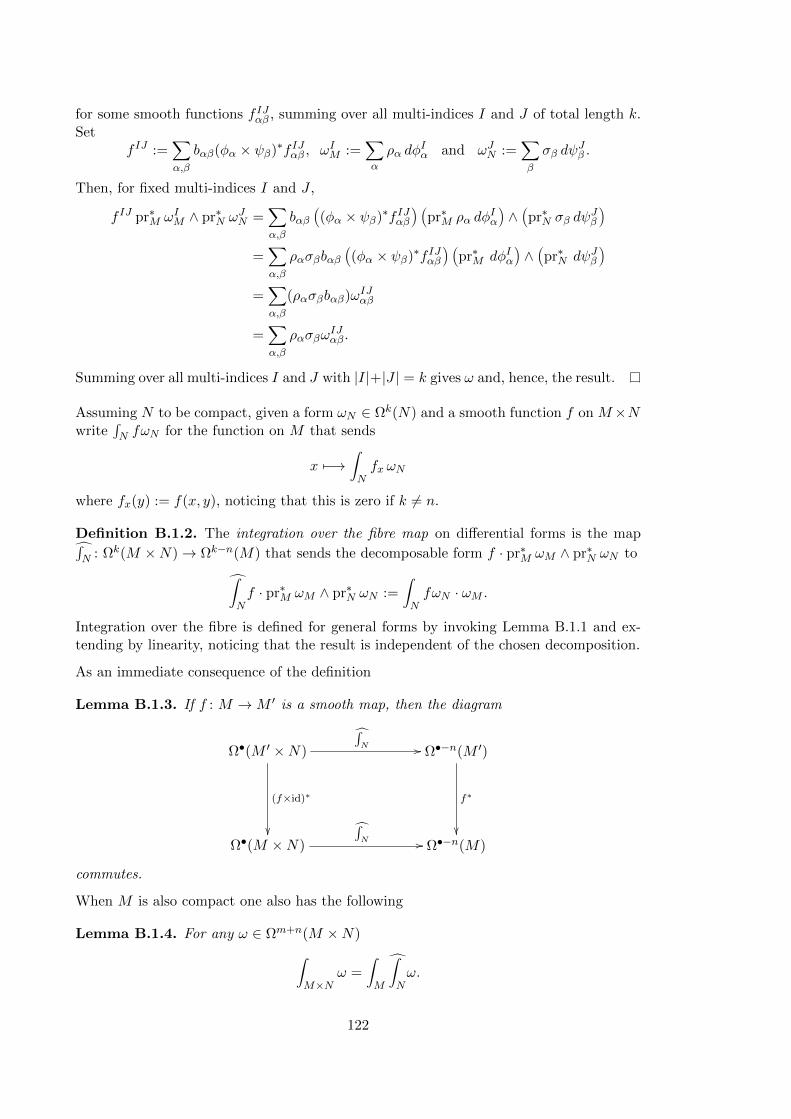
for some smooth functions f IJαβ , summing over all multi-indices I and J of total length k.Set

f IJ :=∑α,β

bαβ(φα × ψβ)∗f IJαβ , ωIM :=∑α

ρα dφIα and ωJN :=

∑β

σβ dψJβ .

Then, for fixed multi-indices I and J ,

f IJ pr∗M ωIM ∧ pr∗N ωJN =

∑α,β

bαβÄ(φα × ψβ)∗f IJαβ

ä Äpr∗M ρα dφ

Iα

ä∧Äpr∗N σβ dψ

Jβ

ä=∑α,β

ρασβbαβÄ(φα × ψβ)∗f IJαβ

ä Äpr∗M dφIα

ä∧Äpr∗N dψJβ

ä=∑α,β

(ρασβbαβ)ωIJαβ

=∑α,β

ρασβωIJαβ.

Summing over all multi-indices I and J with |I|+|J | = k gives ω and, hence, the result.

Assuming N to be compact, given a form ωN ∈ Ωk(N) and a smooth function f on M×Nwrite

∫N fωN for the function on M that sends

x 7−→∫Nfx ωN

where fx(y) := f(x, y), noticing that this is zero if k 6= n.

Definition B.1.2. The integration over the fibre map on differential forms is the map”∫N : Ωk(M ×N)→ Ωk−n(M) that sends the decomposable form f · pr∗M ωM ∧ pr∗N ωN to”∫

Nf · pr∗M ωM ∧ pr∗N ωN :=

∫NfωN · ωM .

Integration over the fibre is defined for general forms by invoking Lemma B.1.1 and ex-tending by linearity, noticing that the result is independent of the chosen decomposition.

As an immediate consequence of the definition

Lemma B.1.3. If f : M →M ′ is a smooth map, then the diagram

Ω•(M ′ ×N) Ω•−n(M ′)

Ω•(M ×N) Ω•−n(M)

∫N //

f∗

(f×id)∗

∫N //

commutes.

When M is also compact one also has the following

Lemma B.1.4. For any ω ∈ Ωm+n(M ×N)∫M×N

ω =

∫M

”∫Nω.

122

This is proved using the local decompositions of Lemma B.1.1 and Fubini’s Theorem onRm × Rn.

Importantly for constructing integration over the fibre maps in de Rham cohomology, inthe case where N is without boundary one also has

Lemma B.1.5. The integration over the fibre map commutes with the exterior derivative,that is ”∫

Nd = d

”∫N.

Proof. As both ”∫N and d are linear, it suffices to prove the result for decomposable forms.Taking coordinate charts and partitions of unity exactly as in Lemma B.1.1, let ω be adecomposable form on M ×N . Then, for some fixed multi-indices I and J ,

ω =∑α,β

ρασβ (φα × ψβ)∗Äfαβ dx

I ∧ dyJä.

Writing gαβ = (φα × ψβ)∗fαβ and taking the exterior derivative, one obtains

dω =∑α,β

[gαβσβdρα + gαβραdσβ + ρασβdgαβ] ∧ dφIα ∧ dψJβ

=∑α,β

ñgαβσβdρα + gαβραdσβ + ρασβ

m∑i=1

∂gαβ∂φiα

dφiα + ρασβ

n∑j=1

∂gαβ

∂ψjβdψjβ

ô∧ dφIα ∧ dψJβ .

If |J | = n integrating over the fibre gives”∫Ndω =

∑α,β

ñ ∫Nσβgαβ dψ

Jβ · dρα + ρα

m∑i=1

∫Nσβ

∂gαβ∂φiα

dψJβ · dφiαô∧ dφIα

=∑α,β

ñ∫Nσβgαβ dψ

Jβ · dρα + ρα · d

Ç∫Nσβgαβ dψ

Jβ

åô∧ dφIα

=∑α,β

d

ïρα

∫Nσβgαβ dψ

Jβ

ò∧ dφIα

= d”∫Nω

as required. If |J | < n then”∫Ndω =

∑α,β

(−1)|I|ρα

∫N

ñgαβ dσβ ∧ dψJβ + σβ

n∑j=1

∂gαβ

∂ψjβdψjβ ∧ dψ

Jβ

ô· dφIα

=∑α,β

(−1)|I|ρα

∫Nd(σβgαβ ∧ dψJβ ) · dφIα

= 0

using Stokes’ Theorem, since N is without boundary. On the other hand,”∫Nω = 0 =⇒ d

”∫Nω = 0.

Since the result is clearly true for |J | > n (as this implies ω = 0), the result is proved.

123

This implies that there is a well-defined integration over the fibre map in de Rham coho-mology, namely ”∫

N: Hk

deR(M ×N) −→ Hk−ndeR (M)

given by ”∫N

: [ω] 7−→ñ”∫Nω

ô.

By Lemma B.1.3, the diagram

H•deR(M ′ ×N) H•−ndeR (M ′)

H•deR(M ×N) H•−ndeR (M)

∫N //

f∗

(f×id)∗

∫N //

commutes for any smooth map f : M →M ′.

B.2 For singular cohomology

One can also define integration over the fibre for singular cohomology with coefficients inany ring R. The construction, which is necessarily algebraic, relies on a choice of crossproduct for singular chains. The underlying principle is similar to that of the de Rhamisomorphism theorem, in which integration of differential forms is viewed as an algebraicoperation.

Let 4n denote the standard n-simplex in Rn+1. Following [23, pp. 277–278], one nowoutlines how to define a product on singular chains

× : Cm(M ;R)⊗ Cn(N ;R)→ Cm+n(M ×N ;R).

The crucial ingredient is that there is a natural decomposition of the product 4m ×4n

into (m + n)-simplices given as follows. Label the vertices of 4m by v0, . . . , vm and thevertices of 4n by w0, . . . , wn. Thinking of pairs (i, j) with 0 ≤ i ≤ m and 0 ≤ j ≤ n aspoints on an m×n grid in R2, let γ be any path from (0, 0) to (m,n) formed by a sequenceof upward or rightward edges in this grid. To any such path γ one associates the linearmap

`γ : 4m+n −→ 4m ×4n

given by sending the k-th vertex of 4m+n to (vik , wjk), where (ik, jk) is the k-th vertex ofthe path γ. Write |γ| for the number of squares of the grid lying below the path γ.

If a : 4m →M and b : 4n → N are singular simplices in M and N respectively, define

a× b :=∑γ

(−1)|γ|(a× b) `γ , (B.2.1)

which is a singular (m + n)-chain in M × N and the sum ranges over all ‘edgepaths’ γ.This defines the simplicial product on homogeneous elements of Cm(M ;R) ⊗ Cn(N ;R),

124

which is extended to all elements by linearity. Notice that the product × means differentthings on both sides of the equation (B.2.1): on the left hand side it denotes the simplicialproduct and on the right hand side it denotes the product map a×b : 4m×4n →M×N .

From the definition of the singular chain product, it is easy to verify that if f : M → M ′

and g : N → N ′ are continuous maps and a ∈ Cm(M) and b ∈ Cn(N) then

(f × g)∗(a× b) = f∗a× g∗b.

Moreover one can show

∂(a× b) = ∂a× b+ (−1)ma× ∂b

so that the product of two cycles is a cycle and the product of a cycle with a boundary isa boundary. Thus the simplicial product induces a product on singular homology.

Definition B.2.1. The slant product of u ∈ Cm+n(M × N ;R) and z ∈ Cn(N) is thesingular cochain u/z ∈ Cm(M ;R) given by

u/z (c) := u(c× z)

for c ∈ Cm(M).

The interaction of the slant product with the coboundary operator is given by

Lemma B.2.2. For any u ∈ Cm+n(M ×N ;R) and z ∈ Cn(N)

δ(h/z) = δh/z + (−1)mh/∂z.

Proof. For any c ∈ Cm+1(M)

δ(h/z)(c) := h(∂c× z)= h(∂c× z) + ((−1)m + (−1)m+1)h(c× ∂z)= h (∂(c× z)) + (−1)mh(c× ∂z)= δh/z + (−1)mh/∂z

as required.

Thus, the slant product on (co)chains induces the slant product in (co)homology

/ : Hm+n(M ×N ;R)⊗Hn(N) −→ Hm(M ;R).

One is now able to define integration over the fibre for singular cohomology. Take N tobe without boundary, with z ∈ Hn(N) the fundamental class of N .

Definition B.2.3. The integration over the fibre map for singular cohomology is the map”∫N : Hk(M ×N ;R)→ Hk−n(M ;R) given by”∫

Nu := u/z.

125

Following the above discussion, one notices that for any continuous map f : M →M ′ theintegration over the fibre map for singular cohomology fits into the commuting diagram

H•(M ′ ×N ;R) H•−n(M ′;R)

H•(M ×N ;R) H•−n(M ;R)

∫N //

f∗

(f×id)∗

∫N //

It is interesting to examine how differential forms behave under the slant product whenviewed as singular cochains via the integration pairing:

Proposition B.2.4. If the cycle z ∈ Zn(N) represents the fundamental class of N thenfor any ω ∈ Ωm+n(M ×N) one has

ω/z =”∫Nω.

Proof. Compare with [19, Lemma 2.4.9]. From the outset, one may suppose that ω is adecomposable form, so that ω = f · ωM ∧ ωN (suppressing the pullback maps). Writez =

∑i ziσi for some singular n-simplices σi : 4n → N . For any singular m-simplex

c : 4m →M

ω/z (c) :=∑i

zi ω(c× σi)

=∑i

zi (c× σi)∗ω(idm× idn)

=∑i

zi

∫idm× idn

(c× σi)∗ω

where idm, idn denote the identity maps on 4m, 4n respectively so that idm× idn isa singular (m + n)-chain in 4m × 4n. Even though idm× idn is not the identity on4m×4n, by construction of the simplicial product it is a decomposition of 4m×4n into(m+ n)-simplices whose orientations cancel on internal faces. Thus

∑i

zi

∫idm× idn

(c× σi)∗ω =∑i

zi

∫4m×4n

(c× σi)∗ω

=∑i

zi

∫4m×4n

(c× idn)∗(idm×σi)∗ω

=∑i

zi

∫4m

‘∫4n

(c× idn)∗(idm×σi)∗ω

=∑i

zi

∫4m

c∗‘∫4n

(idm×σi)∗ω,

where the third line invokes Lemma B.1.4 and the fourth line invokes Lemma B.1.3. Noticethat for any x ∈ 4m

(idm×σi)∗fx = σ∗i fx

126

so that, recalling the definition of the integration over the fibre map for differential forms,one has

∑i

zi

∫4m

c∗‘∫4n

(idm×σi)∗ω =∑i

zi

∫c

Ç∫4n

σ∗i (fωN ) · ωMå

=

∫c

(∑i

zi

∫σi

fωN

)ωM

=

∫c

Å∫zfωN

ãωM

=

∫c

Å∫NfωN

ãωM

=”∫Nω (c),

where the fourth line follows since z represents the fundamental class of N . Since every-thing in sight is linear, one has

ω/z (c) =”∫Nω (c)

for any c ∈ Cm(M) and, hence, the result.

127

Appendix C

Differential extensions

This appendix provides the background material on differential extensions required forthe discussion of differential K-theory in Chapter 4. The basic idea is that a differentialextension of a cohomology theory combines cohomological information with differentialform data in a non-trivial fashion.

Differential extensions of generalised cohomology theories are described by a relativelysmall set of axioms, originally proposed in [5] and outlined below. Following the axioms,some useful results are recorded. For a comprehensive review of differential extensions,particularly differential K-theory, see [7].

C.1 Axioms for differential extensions

When dealing with differential extensions, the starting point is the generalised (Eilenberg-Steenrod) cohomology theory that one wishes to extend. Suppose that E is a generalisedcohomology theory equipped with a natural transformation

ch : E(X) −→ H(X;V )

called the Chern character of E, where V is some graded R-vector space and H(X;V ) issingular cohomology with coefficients in V .

Definition C.1.1 ([7]). A differential extension of the pair (E, ch) is a functor

M 7−→ E(M)

from the category of smooth compact manifolds (with corners) to the category of Z-gradedgroups together with the natural transformations

1. R : E(M) −→ Ωd=0(M ;V ) := Ωd=0(M)⊗R V (the curvature);

2. cl : E(M) −→ E(M) (the underlying class); and

3. a : Ω(M ;V )/im d −→ E(M) (the action of forms),

with d the usual exterior derivative. The natural transformations R, cl and a are requiredto satisfy

129

1. the diagram

E(M) E(M)

Ωd=0(M ;V ) H(M ;V )

cl //

ch

R

deR //

commutes, with deR the map induced by the de Rham isomorphism;

2. R a = d;

3. a is of degree 1; and

4. the sequence

E•−1(M)ch−−−→ Ω•−1(M ;V )/im d

a−−→ E•(M)cl−−→ E•(M) −→ 0 (C.1.1)

is exact.

Example C.1.2. As a first example of a differential extension, observe that any characterfunctor (Definition 2.2.1) defines a differential extension of integral singular cohomology.The Chern character in this case is the map HZ→ HR induced by the coefficient inclusionZ → R.

In the case that the underlying cohomology theory E is multiplicative (i.e. is valued inZ-graded rings) and the Chern character is a homomorphism of graded rings, one can alsorequire that a differential extension also respects the ring structure.

Definition C.1.3 ([7]). A differential extension E of a multiplicative cohomology theory(E, ch) is multiplicative if

1. E is a functor to Z-graded rings;

2. R and cl are multiplicative; and

3. a(ω) · x = a(ω ∧R(x)) for all x ∈ E(M) and ω ∈ Ω(M ;V )/im d, with · the producton E(M).

Example C.1.4. The differential characters of Cheeger-Simons (Definition 2.2.4) give amultiplicative differential extension of ordinary integer-valued singular cohomology.

There is a special pushforward map for differential extensions that plays a central role inobtaining the Bunke-Schick uniqueness results. Observe that any generalised cohomologytheory E has an S1-integration map∫

S1: E•(M × S1) −→ E•−1(M),

that plays the role of the suspension map (see [6, Section 1] or p. 107). Passing todifferential extensions, the corresponding extra structure is

Definition C.1.5. A differential extension E of (E, ch) has S1-integration if there is anatural transformation ∫

S1: E•(M × S1) −→ E•−1(M)

130

compatible with the natural transformations R and cl and the S1-integration maps ondifferential forms and on E. One also requires

1.∫S1 pr∗M x = 0 for each x ∈ E•(M); and

2.∫S1(idM ×t)∗x = −

∫S1x for all x ∈ E•(M × S1), with t : S1 → S1 the (orientation-

reversing) map given by complex conjugation.

It turns out that under certain mild conditions on the underlying cohomology theory E,any multiplicative differential extension of E has a canonical choice of S1-integration [6, 7].

This section is concluded by recording an important consequence of the axioms. Sincedifferential extensions contain differential form data they are not homotopy invariant ingeneral; the homotopy formula expresses this failure to be homotopy invariant in terms ofdifferential form data.

Theorem C.1.6 (Homotopy Formula). Let E be a differential extension of (E, ch). Ifx ∈ E(M × [0, 1]) and ςt : M →M × [0, 1] is the slice map ςt(x) := (x, t) then

ς∗1x− ς∗0x = a

Ç’∫[0,1]

R(x)

åwhere ‘∫[0,1] denotes integration over the fibre with respect to the canonical orientation on

[0, 1].

For a proof, see [7, Theorem 2.6].

Remark C.1.7. If one suppresses the relevant pullback maps, observe that any form ω onM × [0, 1] is of the form ω = f · α ∧ dt + g · β for some forms α, β on M and smoothfunctions f, g on M × [0, 1]. By Definition B.1.2,’∫

[0,1]ω :=

∫[0,1]

f dt · α

whereas if ∂t is the canonical vector field on [0, 1] and ςt : m 7→ (m, t) is the slice map

∫ 1

0ς∗t ı∂tω dt =

∫ 1

0ς∗t (fα) dt =

∫ 1

0f dt · α =

’∫[0,1]

ω.

The Homotopy Formula may then be restated as

ς∗1x− ς∗0x = a

Ç ∫ 1

0ς∗t ı∂tR(x) dt

å,

which is the form used in Section 4.2.2.

C.2 Uniqueness of differential extensions

The following result on uniqueness of differential extensions is due to Bunke and Schick.It was proved originally in [6] and appears also in [7].

131

Theorem C.2.1 ([6]). Suppose E is a multiplicative generalised cohomology theory thatis rationally even, i.e. E2k−1(pt)⊗Q = 0 for all k, and that Ek(pt) is a finitely-generatedabelian group for all k ∈ Z. Then if E′ and E are any two differential extensions of Ewith S1-integration, there is a unique natural isomorphism E′ → E compatible with all thestructure (including the S1-integration).

If E′ and E do not have S1-integration, there is still a natural isomorphism of the even-degree parts.

If E′ and E are both multiplicative, the natural isomorphism is also multiplicative.

It is important to notice that the S1-integration plays a crucial role in this result. In [6],it is shown that without such a map there is an infinite family of differential extensions ofthe odd-degree part of K-theory that have non-isomorphic group structures.

Observe also that the hypotheses of Theorem C.2.1 are satisfied by topological K-theoryon compact manifolds (with corners), so as a special case one obtains

Theorem C.2.2 ([6]). Suppose K ′ and K are differential extensions of complex K-theory.Then there is a unique natural isomorphism K ′even → Keven compatible with all the struc-ture.

If both extensions are multiplicative this isomorphism extends uniquely to a multiplicativeisomorphism K ′ → K compatible with all the structure.

If both extensions are equipped with S1-integration this isomorphism extends uniquely toan isomorphism K ′ → K compatible with all the structure, including the S1-integration.

Since any two differential extensions of K-theory with S1-integration are uniquely isomor-phic, any such differential extension is called (a model for) differential K-theory. Examplesinclude the Freed-Lott model [15] that uses complex Hermitian vector bundles equippedwith extra form data, the cocycle model of Hopkins and Singer [26], and a model due toBunke and Schick that uses geometric families of Dirac operators [5]. The Simons-Sullivanmodel reviewed at the beginning of Chapter 4 (see also [38]) gives a differential extensionof even K-theory and hence a model for even differential K-theory. For a detailed surveyof existing models of differential K-theory see [7].

132

Bibliography

[1] M. F. Atiyah. K-theory. Lecture notes by D. W. Anderson. W. A. Benjamin, Inc.,New York-Amsterdam, 1967.

[2] A. Borel. Topics in the homology theory of fibre bundles, volume 1954 of Lecturesgiven at the University of Chicago. Springer-Verlag, Berlin, 1967.

[3] R. Bott and L. W. Tu. Differential forms in algebraic topology, volume 82 of GraduateTexts in Mathematics. Springer-Verlag, New York, 1982.

[4] J.-L. Brylinski. Loop spaces, characteristic classes and geometric quantization. Mod-ern Birkhauser Classics. Birkhauser Boston Inc., Boston, MA, 2008. Reprint of the1993 edition.

[5] U. Bunke and T. Schick. Smooth K-theory. Asterisque, (328):45–135 (2010), 2009.

[6] U. Bunke and T. Schick. Uniqueness of smooth extensions of generalized cohomologytheories. J. Topol., 3(1):110–156, 2010.

[7] U. Bunke and T. Schick. Differential K-theory: a survey. In Global Differential Ge-ometry, volume 17 of Springer Proceedings in Mathematics, pages 303–358. Springer,Heidelberg, 2012.

[8] A. L. Carey and M. K. Murray. String structures and the path fibration of a group.Commun. Math. Phys., 141(3):441–452, 1991.

[9] H. Cartan. La transgression dans un groupe de Lie et dans un espace fibre principal. InColloque de topologie (espaces fibres), Bruxelles, 1950, pages 57–71. Georges Thone,Liege, 1951.

[10] J. Cheeger and J. Simons. Differential characters and geometric invariants. In Ge-ometry and topology (College Park, Md., 1983/84), volume 1167 of Lecture Notes inMath., pages 50–80. Springer, Berlin, 1985.

[11] S. S. Chern and J. Simons. Characteristic forms and geometric invariants. Ann. ofMath. (2), 99:48–69, 1974.

[12] J. L. Dupont. Curvature and characteristic classes. Lecture Notes in Mathematics,Vol. 640. Springer-Verlag, Berlin, 1978.

[13] D. S. Freed. Dirac charge quantization and generalized differential cohomology. InSurveys in differential geometry, Surv. Differ. Geom., VII, pages 129–194. Int. Press,Somerville, MA, 2000.

[14] D. S. Freed. Remarks on Chern-Simons theory. Bull. Amer. Math. Soc. (N.S.),46(2):221–254, 2009.

133

[15] D. S. Freed and J. Lott. An index theorem in differential K-theory. Geom. Topol.,14(2):903–966, 2010.

[16] H. Garland and M. K. Murray. Kac-Moody monopoles and periodic instantons.Commun. Math. Phys., 120(2):335–351, 1988.

[17] E. Getzler. The odd Chern character in cyclic homology and spectral flow. Topology,32(3):489–507, 1993.

[18] H. Glockner. Direct limit Lie groups and manifolds. J. Math. Kyoto Univ., 43(1):2–26,2003.

[19] R. Green. A Fourier-Mukai transform for invariant differential cohomology. PhDthesis, University of Adelaide, 2011.

[20] R. S. Hamilton. The inverse function theorem of Nash and Moser. Bull. Amer. Math.Soc. (N.S.), 7(1):65–222, 1982.

[21] V. L. Hansen. Some theorems on direct limits of expanding sequences of manifolds.Math. Scand., 29:5–36, 1971.

[22] R. Harvey, B. Lawson, and J. Zweck. The de Rham-Federer theory of differentialcharacters and character duality. Amer. J. Math., 125(4):791–847, 2003.

[23] A. Hatcher. Algebraic topology. Cambridge University Press, Cambridge, 2002.

[24] J. L. Heitsch and H. B. Lawson, Jr. Transgressions, Chern-Simons invariants and theclassical groups. J. Differential Geometry, 9:423–434, 1974.

[25] P. Hekmati, M. K. Murray, and R. F. Vozzo. The general caloron correspondence. J.Geom. Phys., 62(2):224–241, 2012.

[26] M. J. Hopkins and I. M. Singer. Quadratic functions in geometry, topology, andM-theory. J. Differential Geometry, 70(3):329–452, 2005.

[27] T. P. Killingback. World-sheet anomalies and loop geometry. Nuclear Phys. B, 288(3-4):578–588, 1987.

[28] S. Kobayashi and K. Nomizu. Foundations of differential geometry. Vol. I. WileyClassics Library. John Wiley & Sons Inc., New York, 1996. Reprint of the 1963original, A Wiley-Interscience Publication.

[29] S. Kobayashi and K. Nomizu. Foundations of differential geometry. Vol. II. WileyClassics Library. John Wiley & Sons Inc., New York, 1996. Reprint of the 1969original, A Wiley-Interscience Publication.

[30] John M. Lee. Introduction to smooth manifolds, volume 218 of Graduate Texts inMathematics. Springer, New York, second edition, 2013.

[31] J. W. Milnor and J. D. Stasheff. Characteristic classes. Princeton University Press,Princeton, N. J., 1974. Annals of Mathematics Studies, No. 76.

[32] M. K. Murray and D. Stevenson. Higgs fields, bundle gerbes and string structures.Commun. Math. Phys., 243(3):541–555, 2003.

[33] M. K. Murray and R. F. Vozzo. The caloron correspondence and higher string classesfor loop groups. J. Geom. Phys., 60(9):1235–1250, 2010.

134

[34] J. Nestruev. Smooth manifolds and observables, volume 220 of Graduate Texts inMathematics. Springer-Verlag, New York, 2003. Joint work of A. M. Astashov, A. B.Bocharov, S. V. Duzhin, A. B. Sossinsky, A. M. Vinogradov and M. M. Vinogradov,Translated from the 2000 Russian edition by Sossinsky, I. S. Krasil′schik and Duzhin.

[35] S. Paycha and S. Rosenberg. Traces and characteristic classes on loop spaces. InInfinite dimensional groups and manifolds, volume 5 of IRMA Lect. Math. Theor.Phys., pages 185–212. de Gruyter, Berlin, 2004.

[36] A. Pressley and G. Segal. Loop groups. Oxford Mathematical Monographs. TheClarendon Press Oxford University Press, New York, 1986. Oxford Science Publica-tions.

[37] J. Simons and D. Sullivan. Axiomatic characterization of ordinary differential coho-mology. J. Topol., 1(1):45–56, 2008.

[38] J. Simons and D. Sullivan. Structured vector bundles define differential K-theory. InQuanta of maths, volume 11 of Clay Math. Proc., pages 579–599. Amer. Math. Soc.,Providence, RI, 2010.

[39] N. Steenrod. The topology of fibre bundles. Princeton Landmarks in Mathematics.Princeton University Press, Princeton, NJ, 1999. Reprint of the 1957 edition, Prince-ton Paperbacks.

[40] T. Tradler, S.O. Wilson, and M. Zeinalian. An elementary differential extension of oddK-theory. Journal of K-theory: K-theory and its Applications to Algebra, Geometry,and Topology, FirstView:1–31, 4 2013.

[41] R. F. Vozzo. Loop Groups, Higgs Fields and Generalised String Classes. PhD thesis,University of Adelaide, 2009.

135

the caloron correspondence and odd di erential k-theory

Documents