the capacity of color histogram indexing dong-woei lin 2003.3.6 ntut csie
Post on 19-Dec-2015
224 views
TRANSCRIPT
The Capacity of Color Histogram Indexing
Dong-Woei Lin 2003.3.6NTUT CSIE

Outlines
PreliminaryHistogram and spatial informationEffectiveness of histogram
Histogram capacityM. Stricker, The capacity of color histogram indexing, ICCVPR, 1994R. Brunelli, Histograms analysis for image retrieval, Pattern Recognition, 2001

Preliminary 1/4
Color histogramIncorporating spatial information
Color coherence vectorCorrelogram (autocorrelogram)Proposed method
Scale weighted (average distance of pixel pairs)Vector weighted (taking account of angle)

Preliminary 2/4
Performance evaluation (for CBIR)With relevant set through human subject:
Precision:
Recall:
where A(q) and R(q) stands for answer set and relevant set for query image q respectively
)(
)()(
qA
qRqAp
)(
)()(
qR
qRqAr
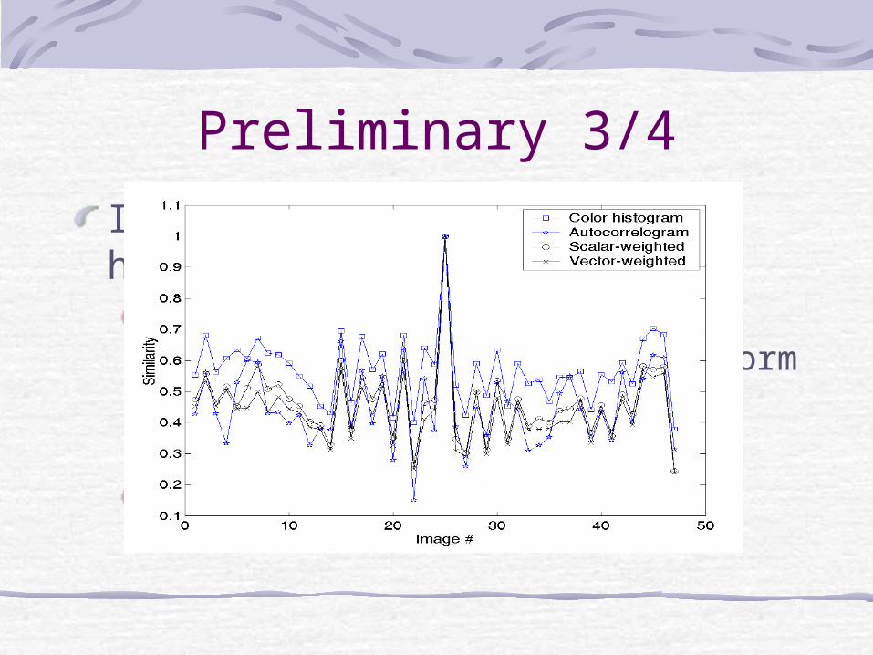
Preliminary 3/4
Improving factor φ(for histogram-based)
Histogram distance and similarity (based on vector norm or PDF)
%100orig
neworig
S
SS
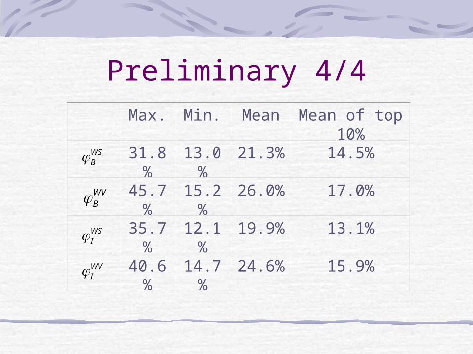
Preliminary 4/4
WSB
WVB
WSI
WVI
Max. Min. Mean Mean of top 10%
31.8% 13.0% 21.3% 14.5%
45.7% 15.2% 26.0% 17.0%
35.7% 12.1% 19.9% 13.1%
40.6% 14.7% 24.6% 15.9%

Histogram Space 1/2
For an image with N pixels, the histogram space ℌ is the subset of an n-dimensional vector space:
ℌ
For a given distance t :t-similar and t-differentIdentical (zero distance)
n
iiin Nhnihhhh
121 ,10,...,,

Histogram Space 2/2
Observations:The interval of reasonable values for t coincides with the first interval on the distance distribution increases very rapidlyIndexing by color histograms works only if the histogram are sparse, i.e., most of the images contain only a fraction of the number of colors of the color space

The Capacity of Histogram Space 1/5
Definition of histogram capacity:C(ℌ, d, t), for a n-dimensional histogram space ℌ, a metric d, and a distance threshold tAssumption: uniform distribution across the color space

The Capacity of Histogram Space 2/5
Theorem:C( , d, t)ℌ maxw,l A(n, 2l, w)
α=(wt/2N) l w n, l n/2A(.) : the maximal number of codewords in any binary code of length nw : constant weight2l : Hamming distance

The Capacity of Histogram Space 3/5
Using (1, 1, …, 0, 0, …, 1) to denote the histogram: a binary word of length n(number of bin) with exactly w 1’s (non-zero bins) in it each 1 represents the pixel number = N/w (w n)2l : the number of bins for two such histogram differ (l w)
n=64, w=62
N/62
11…..01….01..

The Capacity of Histogram Space 4/5
Distance of histogram H1 and H2
for dL1 t, solves l wt/2N =
For any admissible w and l, the maximum of A(.) is still smaller than C
w
NlHHd
LL 211 21
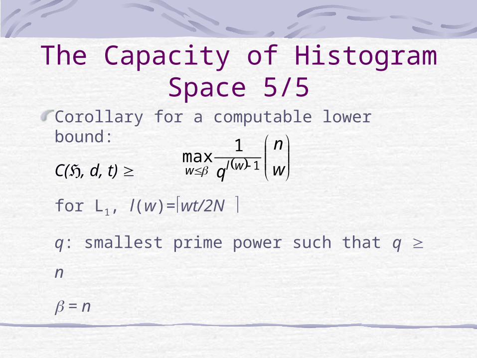
The Capacity of Histogram Space 5/5
Corollary for a computable lower bound:
C( , d, t)ℌ
for L1, l(w)=wt/2N
q: smallest prime power such that q n
= n
w
n
q wlw 1
1max
Histogram analysis for IR
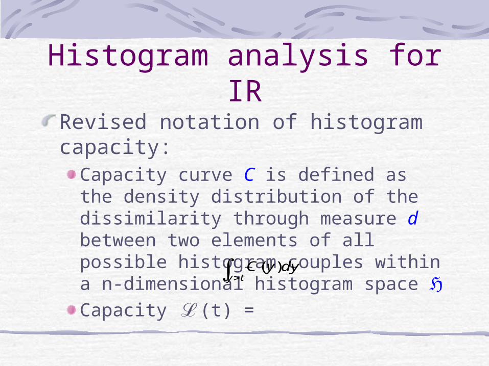
Revised notation of histogram capacity:
Capacity curve C is defined as the density distribution of the dissimilarity through measure d between two elements of all possible histogram couples within a n-dimensional histogram space ℌCapacity (t) = ℒ
tydyyC )(

Histogram analysis for IRTwo major differences from Stricker(94)
No distance function is definedTransforms difficult task “maximal number” into an empirical estimation by considering all image couples within the database
The shape of C(t) Indicator of the distribution of histogramsInduced by the selected dissimilarity measureThe average value of dissimilarity represents the sparseness of histogram space ℌ
Histogram analysis for IR
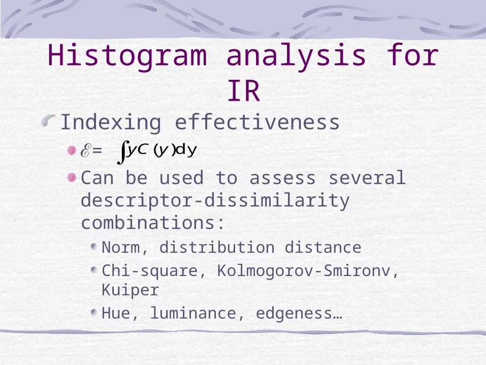
Indexing effectivenessℰ=Can be used to assess several descriptor-dissimilarity combinations:
Norm, distribution distance Chi-square, Kolmogorov-Smironv, KuiperHue, luminance, edgeness…
dy)(yyC
Histogram analysis for IR
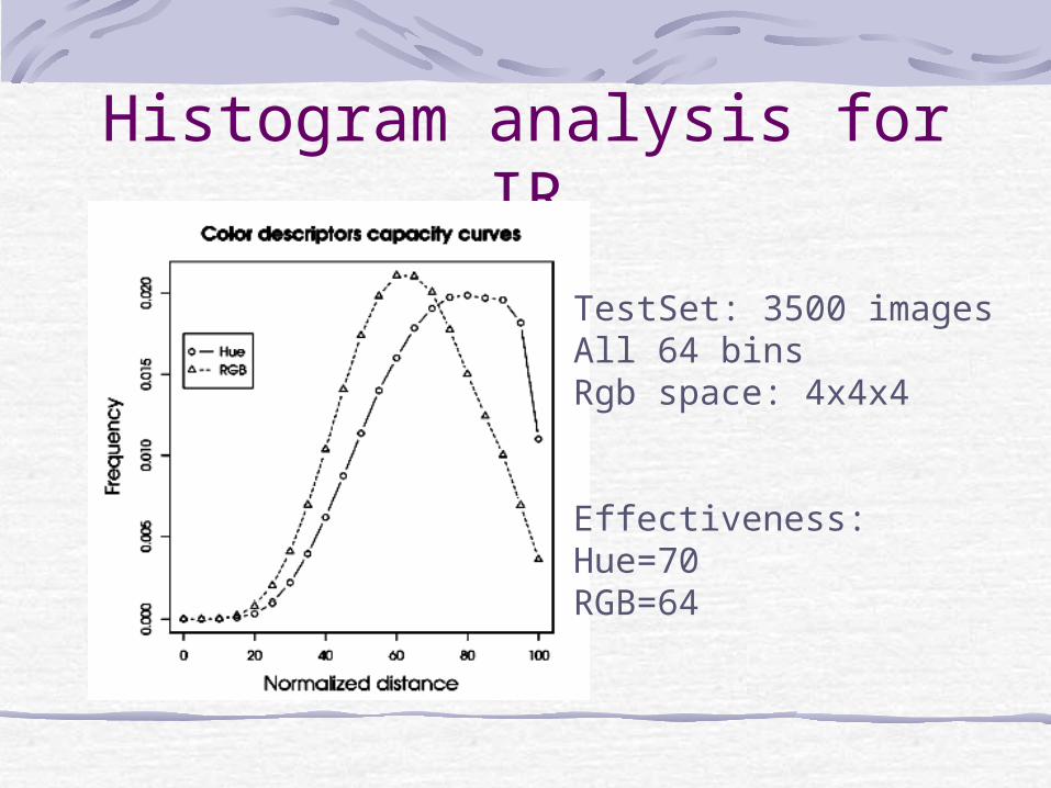
TestSet: 3500 imagesAll 64 binsRgb space: 4x4x4
Effectiveness:Hue=70RGB=64
ExperimentsEstablishments:
RGB color space with 4x4x4 quantizationTargets:
Original image(uncompressed)DC imageDC image with scalar-weightedAutocorrelogram of DC image
Test sets:47 320x240 JPEG images150 192x128 JPEG images from Berkeley collections

Incorporating Spatial Info.Using mean dist. of all same-color pixel pairs as weight:
Similarity measure:
Mean value
of DCT block
max
21 |)()(|1
d
IdIdW jj
j
For color j, image I1 I2
,))(,)(min(),( 2121 jjj
jWSI WIpIpIIS For intersection
.)()(),( 2121 j
jjjWSB WIpIpIIS For Bhattacharyya
* For compatible, the similarity will be transformed to dissimilarity* Intersection adopted only for comparison

Incorporating Spatial Info.
Autocorrelogram of DC image:
Color
Dist.
0 0 … 0 1 1 … 1 ……
0 1 … dmax 0 1 … dmax ……
Pair number
pi,j: pair number of color i with distance j
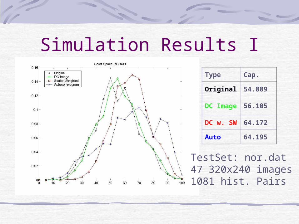
Simulation Results IType Cap.
Original 54.889DC Image
56.105
DC w. SW
64.172
Auto 64.195
TestSet: nor.dat47 320x240 images1081 hist. Pairs

Simulation Results IIType Cap.
Original 58.028DC Image
59.528
DC w. SW
66.823
Auto 68.184
TestSet: ber150.dat150 192x128 images 11175 hist. Pairs

Semi-conclusion
For histogram capacity:Autocorrelogram > scalar-weighted
> DC image > original imageThe shape of autocorrelogramAbout the representation of curve
Spatial Histogram Capacity
Spatial histogram (e.g. edgeness)Assessed features:
E[dist] v.s. color# of pair v.s. pair dist

Simulation Result III
Testset Capacity
nor47 52.715ber150 31.834
nor47 ber150

Consistent of Last Exp.
Considering the number of samples:
Ber150(#) Capacity
50 36.465100 31.447150 31.834

Future Works
Types and properties of spatial histogramStudy spatial descriptorCorrelation of spatial and color featuresSufficiency of definition of effectiveness