the carbon content of austrian trade flows in the european ... filethe carbon content of austrian...
TRANSCRIPT
FIW, a collaboration of WIFO (www.wifo.ac.at), wiiw (www.wiiw.ac.at) and WSR (www.wsr.ac.at)
The Carbon Content of Austrian Trade Flows in the European and International Trade
Context
Birgit Bednar-Friedl, Pablo Muñoz Jaramillo, Thomas Schinko, Karl Steininger
FIW Research Reports 2009/10 N° 05 January 2010
In this study CO2 emissions embodied in Austrian international trade are quantified employing a 66-region input output model of multidirectional trade. We find that Austria’s final demand CO2 responsibilities on a global scale are 38% higher than conventional statistics report (110 Mt-CO2 versus 79 Mt-CO2 in 2004). For each unit of Austrian final demand, currently two thirds of the thus triggered CO2 emissions occur outside Austrian borders. We then develop a 19-region computable general equilibrium model of Austria and its major trading partners and world regions to find that future Austrian climate policy can achieve the EU 20‐20 emission reduction targets, but that its carbon trade balance would worsen considerably. Both unilateral EU and internationally coordinated climate policies affect Austrian international trade stronger than its domestic production.
The FIW Research Reports 2009/10 present the results of four thematic work packages ‘Microeconomic Analysis based on Firm-Level Data’, ‘Model Simulations for Trade Policy Analysis’, ‘Migration Issues’, and ‘Trade, Energy and Environment‘, that were commissioned by the Austrian Federal Ministry of Economics, Family and Youth (BMWFJ) within the framework of the ‘Research Centre International Economics” (FIW) in November 2008.
FIW Research Reports 2009/10
Abstract

The Carbon Content of Austrian Trade Flows in
the European and International Trade Context
Birgit Bednar-Friedl, Pablo Muñoz Jaramillo,
Thomas Schinko, Karl Steininger (coordination)
March 2010
Wegener Center for Climate and Global Change
Karl-Franzens-University of Graz
Study commissioned by the
Austrian Federal Ministry of Economic Affairs, Family and Youth (BMWFJ)
as part of the project ´Research Centre International Economics´ (FIW)


Table of Contents
i
TABLE OF CONTENTS
A Introduction and Overview....................................................................... 7
B The Past and Current Carbon Content of Austrian Trade (Input Output Analysis)……………......................................................................…………………..11
1 Introduction.................................................................................................................12
2 Antecedents of the case study......................................................................................14
3 Methodology ...............................................................................................................17 3.1 MRIO Framework ........................................................................................................ 18 3.2 Data ............................................................................................................................. 20
4 Results .........................................................................................................................22 4.1 A Production‐based Principle versus a Consumption‐Based Principle ....................... 22 4.2 Geographical Analysis ................................................................................................. 24
4.2.1 Regions affected by Austria’s consumption .................................................................... 24 4.3 Sectoral Analysis.......................................................................................................... 26
4.3.1 CO2 drivers at sectoral level............................................................................................. 26 4.3.2 Affected sectors due to domestic and foreign final demand .......................................... 28 4.3.3 Global Path Analysis in a Service Sector .......................................................................... 30
5 Discussion and final comments ....................................................................................33
6 References ...................................................................................................................35
7 Annex ..........................................................................................................................38
C Post Kyoto Climate Policies and their Impact on the Carbon Content of Austrian Trade (Computable General Equilibrium Analysis)........................... 43
1 Introduction.................................................................................................................43
2 Data sources for the modeling framework ...................................................................45 2.1 Economic and trade data and its sectoral and regional aggregation ......................... 45 2.2 Energy and emissions.................................................................................................. 47 2.3 Economic dynamics..................................................................................................... 48
3 The model....................................................................................................................50 3.1 Basic model structure ................................................................................................. 50

Carbon Content of Austrian International Trade
ii
3.2 Production structure ................................................................................................... 50 3.3 Trade in the model ...................................................................................................... 53 3.4 Final demand ............................................................................................................... 56
4 Definition of policy scenarios ....................................................................................... 58 4.1 Post‐Kyoto climate policies ......................................................................................... 58 4.2 The BAU 2020 scenario ............................................................................................... 61 4.3 CO2 emissions in the BAU 2020 scenario .................................................................... 64
5 The economic and global carbon effects of climate policy for Austria as an internationally trading economy ......................................................................................... 68 5.1 The economic effects of the climate policy scenarios for Austria .............................. 68
5.1.1 Effects on Austrian output............................................................................................... 69 5.1.2 Effects on Austrian exports.............................................................................................. 71 5.1.3 Effects on Austrian imports ............................................................................................. 74
5.2 The carbon effects of the scenarios for Austria .......................................................... 76 5.3 The economic and carbon effects of the scenarios on a global scale ......................... 81
5.3.1 The effects on GDP .......................................................................................................... 82 5.3.2 The carbon markets: emissions, prices and decarbonization.......................................... 83 5.3.3 Carbon Leakage................................................................................................................ 90
6 Alternative policy scenarios ......................................................................................... 97
7 Conclusions ............................................................................................................... 103
8 References................................................................................................................. 107

Table of Contents
iii
LIST OF FIGURES
Figure 2‐1: CO2 emissions on the basis of PBP and main macroeconomic aggregates for the years 1970‐2006 in Austria (index 1990=100)........................................................................................15
Figure 2‐2: Austria’s CO2 intensities for the period 1960‐2006 (Index, 1990=100). ..........................16
Figure 4‐1: CO2 flows embodied in Austria’s imports per region in the year 1997 and 2004 in thousands of tons..........................................................................................................................25
Figure 4‐2 CO2 flows embodied in Austria’s exports per region in the year 1997 and 2004 (in thousands of tons) ........................................................................................................................26
Figure 4‐3: Emissions embodied in Austria's final domestic consumption by sectors and place of origin, domestic or foreign territory in 2004 (in thousands of tons) ............................................27
Figure 4‐4: Domestic emissions embodied in the top 15 exports in 2004 (in thousands of tons of CO2) ...............................................................................................................................................27
Figure 4‐5 Top 15 sectors most affected by domestic consumption and exports (in thousands of tons) ..............................................................................................................................................29
Figure 4‐6: Top 15 of the most affected industries abroad due to Austrian final consumption (in thousands of tons) ........................................................................................................................29
Figure 4‐7: Global path at regional and sectoral level for the public service sector, which embodied the largest amount of C02 of the imported commodities ............................................................31
Figure 3‐1: Nesting structure of primary energy extraction...............................................................51
Figure 3‐2: Production of non‐primary energy commodities.............................................................53
Figure 3‐3: Armington aggregation for country r ...............................................................................54
Figure 3‐4: Import structure for country r..........................................................................................55
Figure 3‐5: International Transport ....................................................................................................55
Figure 3‐6: Final demand of private households for country r...........................................................56
Figure 4‐1: PBP vs. CBP in 2004 and 2020 (in Mt CO2) .......................................................................66
Figure 5‐1: Output of ETS sectors for 2020 (in MUSD).......................................................................70
Figure 5‐2: Output of non‐ETS sectors for 2020 (in MUSD) ...............................................................71
Figure 5‐3: Austrian exports of ETS sectors by region for 2020 (in MUSD)........................................72
Figure 5‐4: Austrian exports of non‐ETS sectors by region for 2020 (in MUSD) ................................73
Figure 5‐5: Austrian imports of ETS sectors by region for 2020 (in MUSD) .......................................75
Figure 5‐6: Austrian imports of non‐ETS sectors by region for 2020 (in MUSD)................................75
Figure 5‐7: PBP vs. CBP CO2 emissions for Austria 2020 (Mt CO2) .....................................................77
Figure 5‐8: CO2 according to CBP for Austria 2020 (Mt CO2) .............................................................78
Figure 5‐9: CO2 emissions in AUT trade 2020 (Mt CO2)......................................................................79
Figure 5‐10: Change in CO2 emissions (in Mt CO2) per region and per scenario relative to 2004 .....84
Figure 5‐11: CO2 coefficients for BAU 2020 across countries and sectors (t CO2/MUSD)..................88
Figure 5‐12: CO2 coefficients for ELY sectors across countries and scenarios (t CO2/MUSD) ............89
Figure 5‐13: CO2 effects (in Mt CO2) in abating and non‐abating regions relative to BAU‐2020 .......92
Figure 5‐14: Change in CO2 emissions (in Mt CO2) relative to BAU....................................................93
Figure 6‐1: Trade effects of BTA in the ETS_EU scenario (in MUSD) relative to BAU.........................98
Figure 6‐2: CO2 effects of BTA in the ETS_EU scenario (in MUSD) relative to BAU..........................100
Carbon Content of Austrian International Trade
iv
LIST OF TABLES Table 4‐1: Austria’s CO2 responsibilities: Emissions embodied in different categories (in thousands
of tons of CO2)............................................................................................................................... 23
Table 7‐1: Multidirectional, uni‐directional, and autonomous models applied to the Austrian case for the year 2004. GTAP V7 was used........................................................................................... 38
Table 7‐2 CO2 flows embodied in Austrian imports per region for the years 1997 and 2004 in thousands of tons ......................................................................................................................... 39
Table 7‐3: CO2 flows embodied in Austrian exports per region for the years 1997 and 2004 in thousands of tons ......................................................................................................................... 40
Table 7‐4: CO2 drivers at sectoral level and affected sectors due to domestic and foreign final demand in 2004 ............................................................................................................................ 41
Table 2‐1: Overview of regions .......................................................................................................... 45
Table 2‐2: Overview of sectors........................................................................................................... 46
Table 2‐3: Annual Growth rates 2004 – 2020 .................................................................................... 49
Table 3‐1: Elasticities in production ................................................................................................... 52
Table 3‐2: Armington elasticities (telaes)............................................................................................ 54
Table 3‐3: Elasticities in import structure .......................................................................................... 56
Table 4‐1: GHG emission reduction targets for 2020......................................................................... 59
Table 4‐2: GHG emission reduction targets for 2020 relative to 2004 .............................................. 60
Table 4‐3: BAU 2020 scenario for Austria (in million USD, below: MUSD) ........................................ 62
Table 4‐4: Austrian trade flows in the BAU 2020 scenario (in MUSD) ............................................... 64
Table 4‐5: CO2 emissions for Austria according to the PBP and CBP for 2004 and BAU‐2020........... 64
Table 4‐6: BAU‐2020 scenario – Sectoral CO2 emissions for output, exports and imports for Austria (in Mt CO2) .................................................................................................................................... 67
Table 5‐1: GDP effects of climate policy scenarios for Austria relative to BAU 2020 ........................ 69
Table 5‐2: Sectoral output effects of climate policy scenarios for Austria, 2020 with policy relative to BAU 2020.................................................................................................................................. 70
Table 5‐3: Effects of the scenarios on Austrian exports by sector relative to BAU 2020................... 72
Table 5‐4: Impacts of climate policy scenarios on Austrian exports in ETS and non‐ETS sectors by world region (in MUSD) ................................................................................................................ 73
Table 5‐5: Effects of climate policy scenarios on Austrian imports by sector relative to BAU 2020 . 74
Table 5‐6: Effects of the scenarios on Austrian imports in ETS and non‐ETS sectors by world region (in MUSD)...................................................................................................................................... 76
Table 5‐7: CO2 effects according to the PBP and CBP of the scenarios relative to BAU 2020 ........... 77
Table 5‐8: Sectoral CO2 effects of the scenarios relative to BAU 2020 (Mt CO2)............................... 79
Table 5‐9: Annual GDP growth rates for 2020 for the scenarios ....................................................... 81
Table 5‐10: CO2 emissions (in Mt CO2) per region ............................................................................. 83
Table 5‐11: CO2 price in ETS sectors per region ................................................................................. 85
Table 5‐12: CO2 price in non‐ETS sectors per region.......................................................................... 86
Table 5‐13: CO2 coefficients (in t CO2 per MUSD) per country and sector for BAU 2020.................. 87
Table 5‐14: CO2 coefficients (in tCO2 per MUSD) per country and sector for IPCC_H ....................... 89
Table 5‐15: CO2 effects (in Mt CO2) of climate policies relative to 2004 ........................................... 90
Table 5‐16: Climate policies and carbon leakage ‐ Global CO2 effects relative to 2020 (in Mt CO2) . 91
Table 5‐17: Change in emissions (in %) relative to BAU..................................................................... 93

Table of Contents
v
Table 5‐18: Sectoral CO2 effects and carbon leakage (in Mt CO2) relative to BAU ............................94
Table 5‐19: Sectoral carbon leakage rates .........................................................................................95
Table 6‐1: CO2 price in ETS sectors in Europe.....................................................................................97
Table 6‐2: Output and trade effects of BTA and a non‐uniform carbon price for Austria .................99
Table 6‐3: CO2 effects of BTA and a non‐uniform carbon price for Austria......................................100
Table 6‐4: Global CO2 effects of BTA (in Mt CO2) .............................................................................101


A Introduction and Overview
7
A INTRODUCTION AND OVERVIEW
Climate change mitigation requires a rapid decrease of global emissions of greenhouse gases
(GHGs) from their present value of 8.4 GtC/year to – as of current knowledge –about 1
GtC/year by the end of the century. Facing world economic growth which to date was
enhancing emissions this poses a substantial challenge (Grossmann et al., 2009, Meinshausen
et al., 2009).
International negotiations and agreements (such as the UNFCC Kyoto Protocol) on greenhouse
gas emission reduction have established respective emission accounting systems for countries
(or group of countries). This accounting framework is based on the so‐called ‘Production‐Based
Principle’ (PBP) in which environmental responsibilities are restricted to geographical borders.
This means that indicators only capture the environmental impacts linked to the production of
national goods and exports. Actual emission responsibility by consumption and investment by
individual countries may deviate from the picture drawn by the former accounting systems.
Accounting for emissions on basis of the ‘Consumption‐based Principle’ (CBP) implies
reattributing embodied environmental impacts associated with exports to foreign countries,
and to add to domestic environmental responsibilities those impacts which take place abroad.
For more details about PBP and CBP, see Lenzen et al. (2007), Munksgaard et al. (2001) and
Wiedmann et al. (2007).
Deviations between PBP and CBP measures can result from international trade and the grey
energy and emissions it involves. For countries with very strict domestic objectives and high
incentives to meet them, outsourcing of energy and emission intensive production can cause
significant deviations, which render the initial policy effort questionable, as we deal with a
global pollutant here. Evidence on recent decarbonization has been queried for some
countries (see Helm et al., 2007, for UK’s case) and the question arises, whether the emissions
records really represent a change towards more sustainable societies or whether countries
create clean and natural environments within their borders, by merely displacing degrading
production beyond their boundaries into other countries with lower environmental standards.
Due to the global character of the climate change phenomenon, the countries’ environmental
responsibilities have therefore to be reconsidered beyond their geographical borders.

Carbon Content of Austrian International Trade
8
While international trade has entered the climate policy agenda only rather recently, there is
indeed a strong mutual relationship between international trade and climate policy, along
both the lines pointed out above and beyond:
• for a global pollutant like CO2, international trade can shift carbon intensive production
to less developed countries (pollution haven hypothesis); this effect is occurring when
raised awareness for pollution in industrialized countries makes them choose binding
reduction targets
in particular:
o when climate policies are implemented partially (i.e. unilaterally instead of
globally), international trade allows for importing carbon intensive products
from non‐implementing countries (so‐called carbon leakage)
o when climate policies are implemented partially, some sectors, and particularly
those very exposed to trade, might experience reduced competitiveness
o due to international trade, countries which limit their emissions might still
import carbon intensive commodities, but these emissions are not counted
according to UNFCCC carbon inventories since they are based on production,
but not consumption
• international trade enables the transfer of clean technologies from industrialized to
developing countries (e.g. via CDM), but also among industrialized countries
• internationally linked carbon markets, such as the EU ETS, can reduce the costs of
pollution abatement and thereby are more cost‐effective than unilateral solutions
Thus, international trade and climate policy are linked in both supportive and opposing ways –
both fields thus necessitate a joint analysis.
The present analysis seeks a quantification of carbon content in Austrian international trade
flows with a focus on EU member states and major world trade blocks across time (1992‐2004)
to have a background evaluation instrument for countries’ Kyoto efforts and achievements.
We do so by an enhanced Input‐Output analysis of Austrian trade flows and their direct and
indirect carbon content.
In our methodological approach, however, we go beyond this enhanced statistical analysis
only, by developing also an evaluation tool – a multiregional computable general equilibrium

A Introduction and Overview
9
model of Austrian trade with its trading partners across the world, and specified energy
balance and carbon emission data for each country and/or world region. We simulate a range
of possible post‐Kyoto policies with this tool and report results. This tool is now available also
for further policy simulations of national or EU climate policy efforts, to evaluate their
respective indirect carbon emission impacts via trade flows.
Since the European Council and Parliament approved the EU 2020 targets of the Energy and
Climate package in December 2008, a further set of policy measures has to be implemented in
Austria. It was thus timely to generate a tool to be able to analyze the indirect emission
implications of policy measures developed to achieve the Austrian 2020 targets.
The purpose of the present report is therefore
• to assess the carbon content of Austrian international trade, using the concept of CO2
embodied in international trade (Peters and Hertwich, 2008)
• to analyze the consequences of envisioned climate policies for the post‐Kyoto era
(both EU stand alone, but also more global solutions), for Austrian trade, output,
transport and carbon emissions, as well as the effects on Austria’s main trading
partners (Germany, Italy, Russia, USA, China) and other world regions (EU, North
America excl. USA, Latin America, different Asian regions, Africa).
To address the first objective, we use a multicountry input output analysis with high sectoral
and regional detail (57 sectors and 113 regions). This method is particularly suitable to
investigate the carbon emissions along the production chain of the commodities, both
domestically and abroad. Moreover, we device and apply a method to consider not only the
direct carbon effects of imported and exported products, but also the indirect ones due to
imports of factors of production and intermediate products. With this method at hand, we can
determine the carbon content of Austrian production, imports and exports and ultimately of
Austrian final demand (=consumption). Thus, the main contribution of this method is in the
analysis of physical commodity flows and their link to emissions with particularly high detail.
The second objective is directed towards the future, namely the assessment of different
climate policy scenarios for the post Kyoto era (climate policy up to 2020). This question can
best be addressed within a Computable General Equilibrium (CGE) framework which is also
based on input output tables but extended by household and government data (taxes,
transfers, expenditures) to construct social accounting matrices. The key characteristic of CGE

Carbon Content of Austrian International Trade
10
models is that they allow to analyze the effects of (exogenous) policy changes by requiring that
all markets (input, output, international trade) clear, e.g. by means of adjustments in prices
and input coefficients (production technologies), at all instances of time.
For our analysis we use the GTAP database (GTAP, 2007) which is unique in its sectoral and
regional coverage of consistent input output and trade tables (113 countries and 57
commodities for the base year 2004). Moreover, GTAP‐E provides an extension on carbon
emissions on a sectoral level for all countries included in GTAP. Despite the impressive scope
of the database, it has some limitations (see, e.g., Peters and Hertwich, 2008): Since data is
contributed by GTAP partners voluntarily, some sources are not the most recent ones; more
significant for our analysis, however, is the adjustment necessary to ensure internationally
consistent input output and trade tables. Moreover, the database used for carbon emissions
varies across GTAP versions and the results are therefore not readily comparable across GTAP
versions. Finally, emissions included are solely based on combustion processes (Lee, 2008),
while process related emissions (which can be substantial for some sectors like refineries) are
not part of the emissions data in GTAP. In our work we had to correct for these shortcomings
in the base data as noted in the respective sections.

B The past and current carbon content of Austrian Trade (Input Output Analysis)
11
B THE PAST AND CURRENT CARBON CONTENT OF AUSTRIAN TRADE (INPUT OUTPUT ANALYSIS)
This section aims at quantifying the CO2 emissions embodied in international trade on the
basis of the Consumption‐Based Principle (CBP) for Austria. At a methodological level, Multi
Regional Input‐Output (MRIO) models are used in order to account for Austria’s CO2
responsibilities on a global scale. Estimates are carried out for the years 1997 and 2004. This
allows assessing effects of the increasing globalization process on carbon reallocation, fostered
by unilateral climate change mitigation policies. In order to estimate the relevance of carbon
leakage, indicators established from a consumption perspective are compared with standard
indicators which are based on the Production‐Based Principle (PBP). Results state that during
1997 CO2 responsibilities based on CBP were 32% larger than those based on PBP; that is, CO2
emissions based on PBP indicator amounted to 67 million tons of CO2 (Mt‐CO2), while CO2
responsibilities based on CBP reported 89 Mt‐CO2. This relation has increased through time: as
the CBP indicator of 2004 was 38% larger than the PBP: PBP indicator reported 79 Mt‐CO2
whilst CBP estimates reported 110 Mt‐CO2. Regarding the origin of the emissions embodied in
imports, it is estimated that about one‐fourth (10 Mt‐CO2) originated in non‐Annex I countries
in 1997. This proportion increased to one‐third (21 Mt‐CO2) by 2004. Due to the divergent
magnitude between CBP and PBP indicators as well as the dimensions of carbon leakage,
results suggest a re‐thinking of the accounting basis in order to properly assign CO2
responsibilities. Otherwise, the unilateral character of undergoing climate change mitigation
policies could partially be undermining emissions responsibilities by reallocating pollution
towards those regions without strict environmental commitments.

Carbon Content of Austrian International Trade
12
1 Introduction
The Nature of the climate change phenomenon demands internationally coordinated action in
order to mitigate greenhouse gas (GHG) emissions. With regard to the stabilization of
greenhouse gas concentration, the United Nations Framework Convention on Climate Change
points out that all societies share common but differentiated responsibilities. The largest share
of historical and current global emissions of greenhouse gases can be traced back to high
income economies while the share of global emissions originating in low and middle income
economies are currently at a low per capita level. The latter, however, will inevitably grow
during the emerging process.
The Kyoto Protocol, the largest international agreement on climate change mitigation, is aimed
at committing a subgroup of high income economies to the reduction of their GHG emissions.
The accounting emission system at the Kyoto Protocol is based on the countries’ geographical
territory, i.e. the environmental responsibilities ‘stop’ at the respective national borders of the
countries (IPCC, 2007). The literature usually refers to this accounting system as the
‘Production‐Based Principle’ (PBP) (Munksgaard and Pedersen, 2001). This means that
indicators only capture the environmental pressures which are linked to the production of
national goods and exports.
However, the so called ‘carbon leakage problem’ emerges when emissions inventories are only
focused on the PBP and when climate change policies are unilaterally imposed by a group of
countries only. There are two core definitions with respect to the carbon leakage problem:
(1) As a policy oriented approach the IPCC defines carbon leakage as “the part of emissions
reductions in Annex I countries that may be offset by an increase of the emissions in the
non‐constrained countries above their baseline levels. This can occur through the
relocation of energy‐intensive production in non‐constrained regions” (IPCC 2007). In
other words, the concept relies on the possibility that a unilateral climate change
mitigation policy oriented towards reducing domestic emissions in one region can increase
emissions in another by the substitution of domestic production due to imports and/or
production relocation (for further details see Reinaud, J. 2008; Dröge, S. 2009; IPCC, 2007).
(2) A descriptive approach used to estimate the carbon leakage deals with past and present
emission flows that are embodied in imports coming from non‐Annex I countries to Annex
I countries. The carbon leakage indicator in this context is often defined as the flows of
emission embodied in imports coming from non‐Annex I countries to an Annex I country
divided by the total emissions according the PBP indicator (Peters and Hertwich 2008a). In

B The past and current carbon content of Austrian Trade (Input Output Analysis)
13
this section of our report we will use this latter approach and the country being taken into
consideration from Annex I parties is Austria,. In the policy part of this report (part D),
however, we will obviously use the policy oriented former definition of carbon leakage.
Due to the carbon leakage problem, recent decarbonization trends for some countries have
been queried (see for instance Helm et al 2007 and Minx, et al 2008 for the case of UK). The
question arises whether recent evidence of decarbonisation in production in some countries
really does represent a change towards more sustainable societies or whether countries are
creating clean and natural environments within their borders, while displacing pollution
beyond their geographical limits into countries with lower environmental standards and
commitments. This shows a rising concern in defining the limits of environmental
responsibilities.
In order to overcome the potential environmental leakage problem, solutions suggest setting
an emission accounting that relies on the consumption based principle (CPB). This implies the
reattribution of embodied environmental pressures associated with exports to foreign
countries, and domestic environmental responsibilities should be complemented by those
impacts that take place abroad. Thus, by use of CBP it is possible to capture environmental
responsibilities across the world, since it takes into account the pollution embodied in the
imported commodities. As Peters and Hertwich (2008) suggest some of the advantages of
using CBP as the evaluation criterion in GHG inventories are that it reduces the importance of
emission commitments for developing countries, increases options for mitigation, encourages
environmental comparative advantage, addresses competitiveness concerns, and naturally
promotes technology diffusion.
The current report section aims at: (a) estimating the carbon content of Austrian trade for the
years 1997 and 2004 on the basis of CPB, and thereby, estimating the corresponding carbon
balances between exports and imports for the two years under analysis;(b) comparing
Austria’s CO2 responsibilities on the basis of CBP and PBP; (c) providing insights about physical
dimensions of the carbon leakage problem between the countries comprising Annex I and non‐
Annex I.
This part of report is organized as follows: the next section gives an overview of Austria’s CO2
responsibilities (from a production perspective) and related socioeconomic indicators along
the last three decades. In section 3, foundations of a Multi‐Regional Input‐Output model are
set out in order to estimate CO2 emissions from CBP. Section 4 shows the results, while
section 5 presents a discussion and concluding remarks.

Carbon Content of Austrian International Trade
14
2 Antecedents of the case study
The current section describes Austrian CO2 emissions and macroeconomic indicators for the
period between 1970 and 2006. Nonetheless, the analysis is focused mainly on the time period
between the years 1990 and 2006 due to international commitments regarding GHG emissions
(Kyoto protocol). The amount of Austria’s CO2 emissions has been steadily increasing. In 1970,
Austria’s CO2 emissions were 46 Mt‐CO2, while between 1990 and 2006 Austria’s CO2
emissions rose from 56.56 million tons of CO2 (Mt‐CO2) to 72.84 Mt‐CO21 (see Figure 2‐1). This
rise represents an increase of 28% (IEA, 2008). The absolute amount of CO2 emitted is far
above the Kyoto protocol target, where the commitment was to reduce CO2 emissions by 13%
with respect to the levels in 1990 by 2008‐12. Furthermore, we see that emissions grew even
at an increased rate (at an annual average of 1.3% for the time period 1970‐1990, while 2% for
1990‐2006 respectively).
For the time period between 1970 and 2006, Austria’s economy2 has grown by about 2.5%
percent per year. This means that the GDP has almost doubled twice over the span of 36 years.
Furthermore, exports are an important driving force of economic growth, as they show an
increase of 150% between the years 1990 and 2006, representing around 65% of the GDP in
2006. Concerning Austrian imports, Figure 2‐1 shows a similar development as that of exports
between 1970 and 1997; but grew somewhat slower thereafter. Thus, international trade
represents a substantial component in production and consumption accounts for the small and
open economy of Austria.
1 CO2 figures are based on the IEA because it allows us to observe a longer time period than those
figures based on the UNFCCC. However, it is important to emphasize that the UNFCCC's report of
Austria’s CO2 emissions – due to a more comprehensive coverage – were on average 4.5 Mt‐C02 higher
for each of the years 1990‐2006 than those reported by IEA.
2 Austria is one of the 66 high income economies placed 23th according to the gross national income per
capita measured in purchasing power parity (World Bank 2008).

B The past and current carbon content of Austrian Trade (Input Output Analysis)
15
‐
50
100
150
200
250
300
1970
1972
1974
1976
1978
1980
1982
1984
1986
1988
1990
1992
1994
1996
1998
2000
2002
2004
2006
Exports of goods and services Imports of goods and services
GDP CO2 Sectoral Approach (IEA)
Figure 2-1: CO2 emissions on the basis of PBP and main macroeconomic aggregates for the years 1970-2006 in Austria (index 1990=100).
Source: IEA (2008) and UNdata (2009).
Note: Original monetary data was expressed in constant 1990 and US dollars.
CO2 emissions within the Austrian territory have grown at a slower pace than other indicators
related to production, such as GDP, exports and imports. Thus, it is possible to observe a
tendency towards a relative (but not an absolute) decarbonization of the Austrian economy
with respect to GDP in the time period from 1970 to 2006 (See Figure 2‐2). Notice that this
decarbonization tendency becomes less clear between the years 1990‐2006. Furthermore, as
can be seen in Figure 2‐2, this is partially explained by a relative decrease in the CO2 emissions
per unit of Total Primary Energy Supply (TEPS). Some factors which have contributed to this
last decoupling trend refer to the fact that the total amount of coal supplied to the economy
has been constant throughout the period under analysis, while the relative participation of gas
and, on a smaller scale, of hydropower has increased in total energy supply. In essence, less
CO2 has been emitted per unit of TPES. Concerning CO2 responsibilities per capita, they have
increased over time: in 1970 CO2 emissions per capita were 6.23 tons of CO2, in 1990 CO2
emissions per capita were 8.08 tons CO2, while in 2006 emissions per capita were 9.33 tons
CO2. It is important to emphasize that the indicators stated above refer to carbon emissions
seen from a production perspective only.

Carbon Content of Austrian International Trade
16
0.3
20.3
40.3
60.3
80.3
100.3
120.3
140.3
160.3
1970
1972
1974
1976
1978
1980
1982
1984
1986
1988
1990
1992
1994
1996
1998
2000
2002
2004
2006
CO2 / TPES CO2 / GDP CO2 / Population
Figure 2-2: Austria’s CO2 intensities for the period 1960-2006 (Index, 1990=100).
Source: IEA (2008)
TPES= Total Primary Energy Supply

B The past and current carbon content of Austrian Trade (Input Output Analysis)
17
3 Methodology
A Multi‐Regional Input‐Output (MRIO) model has been chosen as the framework to be used for
accounting CO2 emissions embodied in the commodity bundle that is needed to satisfy a
certain level of consumption for a specific geographic territory. The MRIO competency lies,
among others, on the ability of tracing environmental impacts along the production chain,
from the consumption side backward to the production side. Thus, one attractive feature of
the technique is its ability to establish the production connectedness among sectors and
regions.
MRIO models have had a greater appearance in environmental studies done during the last
decade3, for instance see: Ahmad and Wyckoff (2003); Lenzen et al. (2004); Peters and
Hertwich (2006); Weber and Matthews (2007); Andrew et al. (2008); Giljum et al. (2008);
Peters and Hertwich (2008); Nakano et al. (2008); Wiedmann et al. (2007). In this realm, the
above topics mainly refer to: carbon leakage, natural resource use, CO2 responsibilities,
ecological footprint, and household impacts.
MRIO models can, as Lenzen et al. (2004) points out, be classified in three categories:
autonomous trade, unidirectional trade, and multidirectional trade models. Autonomous
models tend to be – in terms of implementation ‐ the most straightforward approach due to
the low data collection requirements; although, they are also the most restrictive types of
model considering that the underlying assumption states that the import commodities are
produced with the same technology and production structure as that of the importing country.
This assumption is considered usually unrealistic given the high degree of heterogeneous
trading partners which are involved in the world trade system (see for example Machado,
2001; Muñoz et al., in press; among others).
Alternatively, by means of unidirectional models (see for example Ahmad and Wyckoff, 2003;
Peters and Hertwich, 2006; Nakano et al., 2008) it is also possible to trace commodities (and
the emissions embodied in them) back to the producing region, which accounts for its own
technology and economic structure. However, CO2 multipliers only consider emissions emitted
in the exporter country, and neglect emissions embodied in commodities that stem from of a
3 For an extensive review about MRIO models, we refer to Wiedmann et al. (2007) and Wiedmann
(2009).

Carbon Content of Austrian International Trade
18
third region and that are used as intermediate inputs in export commodities. This model leads,
in general, to an underestimation of the CO2 multipliers.
Finally, a multidirectional trade model considers a full feedback loop trade across world
regions induced by the consumer wants of a specific country. Thus, if the domestic
consumption increases for a certain quantity (Austrian consumption in this case), domestic CO2
multipliers and international trade CO2 multipliers estimate the total CO2 responsibilities of this
change in consumption level along the whole production process, across geographical borders
and industries. Domestic CO2 multipliers account for the environmental impacts in the region
where the commodity was produced and consumed. International trade CO2 multipliers
account for the CO2 responsibilities abroad, due to both production abroad and imports to the
country abroad for intermediate use, with the latter further traced back until the ultimate
country/region of origin and its specific emissions.
Thus, multidirectional trade models offer the closest representation of the international trade
system from all three models above because of the explicit modelling of interregional linkages.
The current study has therefore adopted this last concept. The model and data will be
presented in the following subsection and the results are summarized in the subsequent
section. Annex A, however, contains the outcome for all three models tested at an empirical
level for this case study, such that the three modelling approaches and their results can be
compared for the case of Austria.
3.1 MRIO Framework
MRIO is presented for the case of the two regions ‐ r and s ‐ that exchange commodities in one
period of time. Each region produces a certain level of output (x) of industry i. The resulting
output vector represents the total commodities supplied by region r and s. From the demand
side, commodities supplied are used by regions for intermediate use (z), in industry j, and/or
for final demand (y). Thus, the system can be represented by Eq.1:
(1)
1 11 1 11 11 1 11
1 11 11
1 11 1 11 1 1 11
1 1
r rr rr rs rs rr rsn
r rr rr rs rs rr rsn n nn n ns sr sr ss ss sr ss
n n
s sr sr ss ss sr ssn n nn n nn n n
x z z z z y y
x z z z z y yx z z z z y y
x z z z z y y
+ + + + + + +
+ + + + + + +=
+ + + + + + +
+ + + + + + +
…

B The past and current carbon content of Austrian Trade (Input Output Analysis)
19
Equation system (1) allows an understanding of the trade4 interactions between regions and
industries. Additionally, it is possible to define the domestic technical coefficients, ssija or rr
ija ,
and interregional technical coefficients, rsija or sr
ija , as in Eq.2 and Eq.3 respectively:
(2)
(3)
i.e. the technical coefficients reflect the specific amount of commodity input i necessary to
produce one unit of output xj in region r (s), taking into account the input precedence as well
as the place where the output is produced; region r or s. Furthermore, it is possible to
reformulate Eq.1 in terms of the regional and interregional technical coefficients by using block
matrix notation as in Eq. 4:
(4)
Expressing the outputs as a function of the final demands, and the regional and interregional
technical coefficients, the solution of the system in the matrix notation is shown in Eq. (5):
(5)
Rewriting (5) once again in matrix block notation and multiplying the final demands of each
region by the well‐known Leontief inverse Eq.6 is obtained:
(6) r s• •-1 -1x = (I - A ) y + (I - A ) y
where (I-A)-1 provides information about the direct and indirect output changes across regions
and industries due to changes in the final demand in r or s. Vectors y•r and y•s represent the
‘total’ final demand ‐ domestic plus imports ‐ of region r and s respectively. Notice that
(I-A)-1.y.r accounts for the change in production in both regions due to a change in the final
demand of r. The interpretation is similar for region s.
4 Note that exports from r to s are conceptually equal to imports of s from r. In practice, the statistics tend to differ not only due to transport and taxes, but also due to innate discrepancies in trade statistics.
/rr rr rij ij ja z x≡
/rs rs sij ij ja z x≡/sr sr r
ij ij ja z x≡
1r rr rsrr rs
sr sss sr ss
−⎛ ⎞⎛ ⎞ ⎛ ⎞⎛ ⎞⎛ ⎞
−⎜ ⎟⎜ ⎟ ⎜ ⎟⎜ ⎟⎜ ⎟⎜ ⎟ ⎜ ⎟⎜ ⎟⎝ ⎠ ⎝ ⎠⎝ ⎠ ⎝ ⎠⎝ ⎠
x y + yI 0 A A= *
0 I A Ax y + y
/ss ss sij ij ja z x≡
r r rr rsrr rs
sr sss n ss sr
⎛ ⎞ ⎛ ⎞ ⎛ ⎞⎛ ⎞= ∗⎜ ⎟ ⎜ ⎟ ⎜ ⎟⎜ ⎟⎜ ⎟ ⎜ ⎟ ⎜ ⎟⎝ ⎠⎝ ⎠ ⎝ ⎠ ⎝ ⎠
x x y + yA A+
A Ax x y + y

Carbon Content of Austrian International Trade
20
The model can be extended to CO2 impacts in this case (or other variables of interest) by pre‐
multiplying both sides of Eq.(6) by a diagonalized intensity vector of CO2, f̂ , giving sectoral
CO2 emissions divided by sectoral output. The pre‐multiplication of the diagonalized CO2
intensity vector and the Leontief inverse yields CO2 multipliers, i.e. the total, direct and
indirect, increases in CO2 emissions among industries and regions due to a change in final
demand in region r (or s). The resulting formulation is shown in Eq.7:
(7)
where f is the vector of total C02 impacts across regions due to the consumption in y•r and/or
y•s. Additionally, by multiplying the CO2 multipliers matrix with a diagonalized vector of final
demands, column j th of the resulting matrix would give a comprehensive examination of the
CO2 emissions embodied in industry j th by region and sector. Thus, the impacts abroad due to
consumption of one region (imports), as for example the r region, are given by the sum rows in
the rest of the regions (or s in this case), whilst CO2 impacts on region r due to exports would
be given by analyzing consumption in region s. Therefore, it is possible to assign emissions
which take place in other regions to the consumption of one region. The extension of the
model to more regions is deducted in a straightforward way (for further details see, for
example, Miller and Blair, 2009 or Peters, 2004).
3.2 Data
The data base of the Global Trade Analysis Project (GTAP) was used to construct the MRIO
model with full linkages. GTAP provides harmonized Input‐Output tables by country or country
group (multi‐country regions in this case) for the world economy. The current study has used
GTAP version 7 and GTAP version 5 which are set for the years 2004 and 1997, respectively.
Both GTAP versions are homogenous in terms of sectoral disaggregation, consisting of 57
industries per region (see Table 7‐4 for sectoral details). These two GTAP versions, however,
present a different regional disaggregation: GTAP version 7 gives details for 113 regions, while
GTAP version 5 is comprised of 66 regions. Each GTAP version (and therefore each year under
analysis) was treated separately with its own regional disaggregation level in order to avoid
aggregation bias. Nonetheless, the purpose of comparing results from the two years, once the
findings were obtained for the year 2004, leads to the aggregation of these results at the same
regional level as those in 1997 so as to compare CO2 impacts at a regional level for those two
years.
ˆ ˆ ˆs n≡ -1 -1f fx = f (I - A) y + f (I - A) y

B The past and current carbon content of Austrian Trade (Input Output Analysis)
21
Other important issues refer to the construction of bilateral trade matrices and interregional
technical coefficients, i.e. the off‐diagonal blocks in Eq (4). Regarding these issues, GTAP
supplies vectors of sectoral bilateral trade (c) for each pair of the countries by commodity.
However, it does not assist with information about how the bilateral trade imports are used by
the industries at the intermediate use level or final demand. Hence, the import matrices which
are used to allocate the bilateral imports across the industries and the final demand of the
importing country have been utilized.
Thus the off‐diagonal block matrix is calculated as follows:
1ˆrs rs ssij i i ijZ c m M−= and 1ˆsr sr rr
ij i i ijZ c m M−=
where kijM • is the total import matrix of region k (or s and r at the methodological section) by
commodity i and industry j; 1ˆ im− is the row sum of M ; and lkic is the vector of bilateral trade
between region l and k, with k, l= 1,2…113 for GTAP V7 and 1,2…..66 for GTAP V5, and k
different than l. Since each pair of regional bilateral trade is represented by a block matrix, it is
necessary to construct, in the case of GTAP V7 12,656 off‐diagonal blocks (113 regions x 113
regions – 113 diagonal blocks). Notice that the diagonal block is formed by the domestic input‐
output tables of each region, this amount to 113, in the case of GTAP V7. Finally, it is worth
mentioning that this procedure leads us to work with about 41 million of entries ((113 regions
x 57 sectors) x (113 regions x 57 sectors)) for the multiregional intermediate use matrix see
Eq.4. An analogous process was carried out for the year 1997 based on GTAP V5.
GTAP also provides data of CO2 by sector and region with which it fulfils the model data
requirements presented in the previous section. It is also important to mention, however, that
GTAP C02 data refers only to CO2 emissions from fuel combustion. CO2 emissions stemming
from industrial processes have also been included, more precisely the CO2 emissions in the
following processes for all countries reported by UNFCCC (2009): minerals products, chemical
industry and metal production.

Carbon Content of Austrian International Trade
22
4 Results
Results are presented in three different groups. The first group provides aggregate evidence of
the CO2 responsibilities based on the consumption perspective. These results are compared
with those figures derived from applying the production‐based principle. Further macro
indicators such as emissions embodied in exports, imports, and CO2 per capita, are also shown.
Subsequently, results concerning emissions embodied in trade are disaggregated according to
the regions where the CO2 emissions occurred. A similar analysis is carried out for exports,
describing the regions that evoke CO2 emissions in Austria through international trade. Finally,
the analysis given presents and compares both, emissions embodied in the final demand
sectors which drive the emissions in the domestic territory as well as abroad, and those sectors
more affected by consumption in Austria and other regions across the world.
4.1 A Production-based Principle versus a Consumption-Based Principle
In order to allocate the CO2 responsibilities according to the level and composition of
consumption, it is necessary to reattribute embodied environmental impacts associated with
exports to foreign countries, and to add to domestic environmental responsibilities those
impacts which take place abroad but satisfy – via imports – the local consumer needs. Results
of this procedure carried out for the two years under analysis (1997 and 2004) are presented
in Table 4‐1. It is interesting to note that the domestic CO2 emissions embodied in
consumption increased by 5% between the years under study. However, the consumption
level increased by about 11% between the years 1997 and 2004.
The study allows us to observe a relative decoupling trend between consumption and CO2
emissions at domestic level. However, the carbon content of imports which are necessary to
satisfy consumer needs in Austria represents a large fraction of the total impacts: Imports
embodied emissions of 44 Mt‐CO2 in 1997 and 62 Mt‐CO2 in 2004, i.e. if the Austrian final
consumption increases by one unit, then, taking the year 2004 as the reference period, around
two thirds of the CO2 impact of this unit would take place abroad. As a result, CO2 emissions
embodied in imports for consumption are a crucial phenomenon for understanding CO2
responsibilities and decarbonization trends.
Regarding the origin of the emissions embodied in imports, it is important to mention that
about one fourth (10 Mt‐CO2) of them were originated in non‐Annex I countries in 1997. This
proportion increased in the year 2004: emissions emitted in non‐Annex I countries and
triggered by consumers in Austria reached about one third (21 Mt‐CO2) of the total emissions

B The past and current carbon content of Austrian Trade (Input Output Analysis)
23
embodied in imports. These totals are an indicator of the carbon leakage for Austria and a
measure of Austria’s C02 responsibilities in countries without emissions constraints. This
carbon leakage indicator is usually presented as a percentage of the emissions accounted for
under the PBP. In that case, a carbon leakage of 15% and 25% for the years 1997 and 2004,
respectively. The difference between the total emissions embodied in imports and those
originated in non‐Annex I countries were emitted in Annex I countries (see Table 4‐1).
Table 4-1: Austria’s CO2 responsibilities: Emissions embodied in different categories (in thousands of tons of CO2).
Categories and Indicators \Year 1997 2004
Domestic Consumption 44,314 47,780
Consumption in products domestically produced 27,695 29,153
Household (direct consumption) 16,619 18,627
Exports 22,943 31,800
Exports Domestically produced 20,483 27,558
Exports of International Transport 2,460 4,242
Imports (for Austrian Consumption) 44,366 61,988
Imports coming from Annex I countries 34,343 41,408
Imports coming from Non-Annex I countries 10,023 20,581
Imports of International Transport Not available Not available
Indicators
Net Emission Balance (excluding Int. Transport) - 23,884 - 34,430
Consumption-Based Principle (CBP) 88,680 109,768
Production-Based Principle (PBP) 67,257 79,580
Ratio CBP/PBP 1.32 1.38
CO2 Emissions per capita based on PBP (in tons) 8.44 9.74
CO2 Emissions per capita based on CBP (in tons) 11.13 13.42
Note: Emission data on the PBP in this table is based upon process emission data and
fuel combustion emission data, whereas emission data given in section 2 is based on
fuel combustion emissions only (IEA, 2008), as IEA supplies a significantly longer time
series. Emission data on process emissions is taken from UNFCCC, on fuel combustion
emissions from GTAP, with the latter at values between the ones of IEA and UNFCCC.
The export carbon content showed an increase of 9 Mt‐CO2 (39%) from 1997 to 2004, or seen
in absolute levels, the emissions embodied in exports (EEE) rose from about 23 Mt‐CO2 to
about 32 Mt‐CO2. These changes can be explained by an increase in exports of (international)
transport which doubled between 1997 and 2004; while the EEE of commodity production
shows an increase of 7 Mt‐CO2 (39%) (see Table 4‐1). It is interesting to note that the volume
of exports grew by 56% between the years 1997 and 2004 (see Table 4‐1).

Carbon Content of Austrian International Trade
24
Furthermore, for the period between 1997 and 2004, Austrian CO2 emissions increased by
about 12 Mt (18%) based on the PBP5, that is an increase from 67 Mt‐CO2 to 79 Mt‐CO2. If
emissions are accounted for from the consumption perspective, it is found that emissions rose
from 89 Mt‐CO2 to 110 Mt‐CO2 on the consumption basis, representing this as an increase of
24%. Thus, it does certainly matter in the case of Austria whether emissions are measured on
the production or consumption basis. Accounting for emissions on the CBP leads to results
which are 32% larger than those derived from PBP in 1997. This share has been increasing over
time: in 2004 the ratio was already 38%. Indicators of CO2 emissions per capita based on a CBP
suggest adding up four million tons per capita in comparison with production based indicators.
For instance, in 2004 the CO2 emissions per capita were 9 tons of CO2 and 13 tons of CO2 for
the PBP and CBP, respectively. Further details are displayed in Table 4‐1.
Moreover, the estimates carried out for Austria’s CO2 emissions from a consumption
perspective lie in a similar range as the ones of other studies. For example, Peters and
Hertwich (2008b) estimated Austrian emissions embodied in consumption to be 95.9 Mt‐CO2
in the year 20016, whilst estimates by Nakano et al. (2008) refer to 92 Mt‐CO2 for the year
2000.
4.2 Geographical Analysis
4.2 .1 Reg ions a f fec ted by Aus t r ia ’s consumpt ion
Figure 4‐1 shows the top 25 regions where emissions are related to Austrian consumption in
the years 1997 and 2004. This represents 90% of all emissions embodied in Austrian imports.
In general, the analysis exhibits that the regions which are geographically closer, and especially
Germany (DEU), are also the most affected. It is worth mentioning the fast rising trend of the
Former Soviet Union (XSU) and China (CHN) representing the top 2 and top 3 origins of the CO2
emissions. These two regions represent 4% and 3% of all emissions in 1997, while in 2004 they
already account for about 12% and 11%, respectively, of the total emissions abroad. Other
countries are now listed further down in the ranking of the most impacted regions. The CO2
emissions assigned to consumption in Austria significantly decreased, as is the case for Poland
(POL) and United States (USA) (see Table 7‐2 for further details).
5 This amount is irrespective of source, see UNFCCC (2009) or IEA (2008).
6 Although this study and Peters and Hertwich (2008b) have used the same data base, GTAP database
version 6, differences may originate due to some data replacement with regard to the present work, e.g.
different vectors of CO2 and different input‐output tables for some countries as those supplied by GTAP.

B The past and current carbon content of Austrian Trade (Input Output Analysis)
25
‐
2,000
4,000
6,000
8,000
10,000
12,000
DEU XSU CHN XCE USA ITA XME NLD POL XSC XRW IND HUN FRA GBR ESP THA JPN XNF TUR BEL MYS CAN XCM TWN
1997 2004
DEU = Germany; XSU = Former Soviet Union; CHN = China; XCE = Rest of Central European Associates; USA = United States of America; ITA = Italy; XME = Rest of Middle East; NLD = Netherlands; POL = Poland; XSC = Rest of South African Customs Union; XRW = Rest of World; IND = India; HUN = Hungary; FRA = France; GBR = United Kingdom; ESP = Spain; THA = Thailand; JPN = Japan; XNF = Rest of North Africa; TUR = Turkey; BEL = Belgium; MYS = Malaysia; CAN = Canada; XCM = Central America and the Caribbean; TWN = Taiwan;
Figure 4-1: CO2 flows embodied in Austria’s imports per region in the year 1997 and 2004 in thousands of tons
Note: The imports of 2004 served as a criterion for the ranking of the different regions.
4.2 .1 .1 Reg iona l dr ivers o f Aus t r ia ’s CO 2 emiss ions embod ied in expor ts
The analysis also allows identifying those regions whose consumption mainly induces the
discharge in CO2 emissions within the Austrian borders. The top 25 regions are depicted in
Figure 4‐2, while the full range of regions is shown in Table 7‐3. In general, final CO2
responsible regions do not change much along the years being studied, apart from an increase
in Austrian CO2 responsibility of Germany, Italy, and China, and the decreases of that of Japan.

Carbon Content of Austrian International Trade
26
‐
1,000
2,000
3,000
4,000
5,000
6,000
7,000
DEU USA ITA GBR XCE FRA CHE ESP XME XSU NLD JPN CHN HUN XRW BEL POL TUR AUS SWE DNK GRC IND CAN BRA
1997 2004
DEU = Germany; USA = United States of America; ITA = Italy; GBR = United Kingdom; XCE = Rest of Central European Associates; FRA = France; CHE = Switzerland; ESP = Spain; XME = Rest of Middle East; XSU = Former Soviet Union; NLD = Netherlands; JPN = Japan; CHN = China; HUN = Hungary; XRW = Rest of World; BEL = Belgium; POL = Poland; TUR = Turkey; AUS = Australia; SWE = Sweden; DNK = Denmark; GRC = Greece; IND = India; CAN = Canada; BRA = Brazil.
Figure 4-2 CO2 flows embodied in Austria’s exports per region in the year 1997 and 2004 (in thousands of tons)
Note: The exports of 2004 served as a criterion for the ranking of the different regions.
4.3 Sectoral Analysis
4.3 .1 CO 2 dr ivers a t sec tora l leve l
One of the advantages of the MRIO models lies in the ability to estimate CO2 emissions
embodied across industries and regions. Figure 4‐3 presents CO2 emissions embodied in the
top 15 commodity groups (or industries) consumed in Austria in the year 2004, distinguishing,
at the same time, whether CO2 emissions took place in Austria or in the rest of the world.
These 15 (out of 57) commodity groups explain 82% of the emissions based on the
consumption principle, which represents a total amount of 91 Mt‐CO27. Consistent with Table
4‐1, the larger part of the impacts takes place abroad at a sectoral level, with the exception of
electricity, whose CO2 emissions dominate of domestic origin (see Table 7‐4 for details).
7 It is worth noting that these figures only account for emissions embodied in products. This implies that
it is still necessary to consider the sectoral analysis of those sectors which supply directly to the
residential household, as for instance, electricity. Therefore, adding the 91 Mt‐CO2 and the 19 Mt‐CO2
caused by households, the 110 reported by the PBP indicator are obtained (see table 4‐1).

B The past and current carbon content of Austrian Trade (Input Output Analysis)
27
By contrast, Figure 4‐4 represents the top 15 commodities (81% of emissions embodied in
exports (EEE)) which are consumed in the rest of the world but which induce emissions in
Austria. Note the much lower absolute levels depicted for exports of sectors.
0 2000 4000 6000 8000 10000 12000
osg
cns
otp
ome
ely
obs
mvh
crp
trd
ofd
ele
omf
atp
wap
nmm
Domestic Emisssion Embodied in Consumption Emissions Embodied in Imports
Figure 4-3: Emissions embodied in Austria's final domestic consumption by sectors and place of origin, domestic or foreign territory in 2004 (in thousands of tons)
‐ 500 1,000 1,500 2,000 2,500 3,000 3,500
cns
ome
mvh
osg
atp
crp
otp
trd
obs
ely
ofd
ros
ele
omf
fmp
Emissions Embodied in Exports
Figure 4-4: Domestic emissions embodied in the top 15 exports in 2004 (in thousands of tons of CO2)
cns = Construction; ome = Machinery and equipment nec; mvh = Motor vehicles and parts; osg = Public Administration, Defense, Education, Health; atp = Air transport; crp = Chemical, rubber, plastic products; otp = Transport nec; trd = Trade; obs = Business services nec; ely = Electricity; ofd = Food products nec; ros = Recreational and other services; ele = Electronic equipment; omf = Manufactures nec; fmp = Metal products.
osg = Public Administration, Defense, Education, Health; cns = Construction; otp = Transport nec; ome = Machinery and equipment nec; ely = Electricity; obs = Business services nec; mvh = Motor vehicles and parts; crp = Chemical, rubber, plastic products; trd = Trade; ofd = Food products nec; ele = Electronic equipment; omf = Manufactures nec; atp = Air transport; wap = Wearing apparel; nmm = Mineral products nec.
Carbon Content of Austrian International Trade
28
4.3 .2 A f fec ted sec tors due to domest ic and fo re ign f ina l demand
We now shed light on those industries in the Austrian economy which are mainly affected by
domestic and foreign consumption. First, by focusing on the production side, we can see to
which extent sectoral emissions are induced by domestic consumption and exports,
respectively. Second, those sectors abroad that are most (emission) burdened by consumption
in Austria are depicted.
Figure 4‐5 shows the top 15 sectors that are most affected by domestic consumption and
export. These 15 industries comprise 93% (53 Mt) of the CO2 emissions emitted in Austria due
to consumption and exports. There is a similar pattern in the sectors affected by domestic
consumption and exports. At a sectoral level one can observe that of the CO2 emissions of the
top sector, electricity, the majority (around 61%) are due to domestic needs. Similar patterns
are observed for the sectors of public administration, defense, education, health (osg),
construction (cns), and food products (ofd). On the other hand, the emissions in the sectors
ranked third, fifth, seventh and fifteenth (Ferrous metals (i_s); air transport (atp); chemical,
rubber, plastic products (crp); and machinery and equipment (ome)), were predominantly
caused in the production of exported goods and services (see Table 7‐4 for full details of all
sectors).
Finally, Figure 4‐6 displays the top 15 industries abroad that are most affected by Austrian
consumption, which concentrate 93% of the total emissions embodied in imports (for further
details see Table 7‐4).

B The past and current carbon content of Austrian Trade (Input Output Analysis)
29
‐ 2,000 4,000 6,000 8,000 10,000 12,000 14,000 16,000
ely
otp
i_s
nmm
atp
cns
crp
ppp
osg
trd
ofd
omn
p_c
obs
ome
Sectors affected in Austria by Austrian Domestic Consumption Sectors affected in Austria by Austrian Exports
Figure 4-5 Top 15 sectors most affected by domestic consumption and exports (in thousands of tons)
0 5000 10000 15000 20000 25000 30000
ely
otp
i_s
crp
nmm
atp
p_c
obs
gdt
trd
nfm
oil
wtp
ppp
omn
Sectors affected by Austrian Consumption in Rest of the World
Figure 4-6: Top 15 of the most affected industries abroad due to Austrian final consumption (in thousands of tons)
ely = Electricity; otp = Transport nec; i_s = Ferrous metals; nmm = Mineral products nec; atp = Air transport; cns = Construction; crp = Chemical, rubber, plastic products; ppp = Paper products, publishing; osg = Public Administration, Defense, Education, Health; trd = Trade; ofd = Food products nec; omn = Minerals nec; p_c = Petroleum, coal products; obs = Business services nec; ome = Machinery and equipment nec.
ely = Electricity; otp = Transport nec; i_s = Ferrous metals; crp = Chemical, rubber, plastic products; nmm = Mineral products nec; atp = Air transport; p_c = Petroleum, coal products; obs = Business services nec; gdt = Gas manufacture, distribution; trd = Trade; nfm = Metals nec; oil = Oil; wtp = Water transport; ppp = Paper products, publishing; omn = Minerals nec.

Carbon Content of Austrian International Trade
30
4.3 .3 G loba l Path Ana lys is in a Serv ice Sec tor
So far the commodities which embodied the largest amounts of CO2 emissions as well as the
most affected regions and sectors have been identified. This section additionally analyzes the
consumption impact of a specific commodity group in Austria on the rest of the world,
differentiating the regional and sectoral level. With regard to the commodity group, the public
service sector, ‘Public Administration, Defense, Education, Health’ (OSG), has been chosen
since this is the service sector that embodied the largest amount of CO2 in imports. One
interesting reason for investigating this industry is the fact that a service sector usually has a
very low direct CO2 intensity, however, it may bear large quantities of CO2 when the complete
supply chain is considered, including the indirect effects. The scale effect, i.e. the large share of
the OSG sector in the total final demand, is another relevant variable for understanding its
large CO2 impacts.
In 2004, the OSG sector embodied 5.9 Mt‐CO2. This is almost 10% of all emissions embodied in
Austrian imports (see Table 4‐1). The detailed picture of the global path in terms of regions
and sectors affected due to final demand of the national OSG is presented in Figure 4‐7. The
analysis reveals that most of the emissions are explained by the electricity sector which is
heavily affected, independent of the region of origin. Other affected industries (albeit at
different scale varying across regions) are mainly: Transport, Chemicals, Rubber, Plastic
products; Ferrous metals and Mineral products (see Figure 4‐7).

Figure 4-7: Global path at regional and sectoral level for the public service sector, which embodied the largest amount of C02 of the imported commodities
Note: Regions: DEU = Germany; XSU = Former Soviet Union; CHN = China; XCE = Rest of Central European Associates; USA = United States of America; ITA = Italy; XME = Rest of Middle East; NLD = Netherlands; POL = Poland. Sectors: ely = Electricity; otp = Transport nec; i_s = Ferrous metals; crp = Chemical, rubber, plastic products; nmm = Mineral products nec; atp = Air transport; p_c = Petroleum, coal products; obs = Business services nec; gdt = Gas manufacture, distribution; oil = Oil; wtp = Water transport; ppp = Paper products, publishing; omn = Minerals nec.


A Introduction and Overview
33
5 Discussion and final comments
One of the characteristics of the greenhouse effect refers to the fact that no matter in which
geographical region emissions occur, all GHGs contribute to climate and global change.
Unilaterally implementing mitigation policies on climate change could partially be causing
import substitution or relocating energy intensive firms due to competitiveness loss of
domestic producers. This fact should force to assess the effectiveness of domestic climate
change mitigation policies beyond the geographical borders of a country.
Present carbon leakage estimates, as accounted for in this part of the report by following the
most recent methods to identify emissions embodied in trade, indicate that one‐third of the
emissions embodied in Austrian imports were originated in non‐Annex I countries in 2004. It is
important to note that the above carbon leakage indicator is not solely explained by unilateral
climate change policies. There may be other factors, such as a lower wages or the availability
of specific physical resources in non‐Annex I parties, which make the production abroad more
profitable. The indicator reflects the amount of emissions which is Austria, an Annex I country,
responsible for, but which are not subject to any regulation within the UNFCCC accounting
framework yet.
A strong suggestion in this realm refers to a change towards GHG accounting inventories based
on a consumption perspective. As Peters and Hertwich (2008a) argue, one way to overcome
the carbon leakage problem is to use consumption‐based GHG inventories. Other advantages
of this approach over production‐based inventories are to reduce the importance of emission
commitments for developing countries, increase options for mitigation, encourage
environmental comparative advantage, address competitiveness concerns, and naturally
encourage technology diffusion (Peters and Hertwich 2008a).
Alternatively, a part of the literature has been focused on the idea of introducing a carbon
price border adjustment (BA) policy so as to avoid the carbon leakage; i.e. to introduce a tax
according to the carbon content of imported goods from countries without strict GHG
commitments (non‐Annex I parties) (see Reinaud, 2008 and Dröge, 2009). This measure is
somehow oriented to protect potential competitive losses in the domestic industry, preventing
at the same time from inefficient relocations. A weaker suggestion to avoid the carbon leakage
problem has been derived from this approach, which refers to the use of a dual physical
border adjustment policy. Border adjustment could not only be used as a policy instrument to

Carbon Content of Austrian International Trade
34
correct potential competitive losses, but it can also be used as an instrument to account for
the emissions responsibilities of GHG embodied in imports coming from non‐Annex I countries.
Notice that emissions inventories are still based on the PBP and total CO2 responsibilities
across the world are not fully accounted for while exports are still the responsibility of the
exporter country. Nevertheless, this physical border adjustment policy of emission flows is
focussed on the carbon leakage as defined in this section of the report. Emissions embodied in
commodities coming from non‐Annex I are the relevant issue, since their emission
responsibilities are not subject to any international regulation yet, although they are actually in
the responsibility of an Annex I party (i.e. in the responsibility of an Annex I country
consumption). This approach does not focus on the rest of the emissions embodied in imports
coming from Annex I countries nor on exports because they are somehow regulated.
Therefore, GHG responsibilities would stop once the emissions based on PBP plus emissions
embodied from non‐Annex I countries are accounted for, which is therefore including carbon
leakage.
The currently increasing globalization process, the pervasive character of the climate change
phenomenon, the minor historical per capita responsibilities by middle and low income
economies, and hence, their limited participation in global environmental commitments, are
some of the relevant factors which turn the climate change problem into a complex issue. The
figures presented here confirm that unilateral regional initiatives and commitments might fall
short of the targets due to the displacement of emissions, using as a reference an indicator
based only on production. As it has been shown for Austria, a small and very open economy,
the accounting principle used does matter when assigning carbon responsibilities. Therefore,
in order to have a better picture of CO2 responsibilities it is crucial to take into consideration
the relevant aspects resulting from a consumption perspective analysis where countries’
environmental responsibilities go beyond their geographical borders.

B The past and current carbon content of Austrian Trade (Input Output Analysis)
35
6 References
Ahmad, N. and A. Wyckoff. 2003. Carbon dioxide emissions embodied in international trade.
DSTI/DOC(2003)15. Paris: Organisation for Economic Co‐operation and Development.
Dröge, S. 2009. Tackling Leakage in a World of Unequal Carbon Prices. Climate Strategies
Published Reports. 3th November 2009: www.climatestrategies.org.
Giljum, S., C. Lutz, A. Jungnitz, M. Bruckner, and F. Hinterberger. 2008. Global dimensions of
European natural resource use. First results from the Global Resource Accounting Model
(GRAM). SERI Working Paper 7, Sustainable Europe Research Institute, Vienna.
Hayamia, H. and M. Nakamura. 2007. Greenhouse gas emissions in Canada and Japan: Sector‐
specific estimates and managerial and economic implications. Journal of Environmental
Management 85: 371–392.
Helm, D., R. Smale, and J. Phillips. 2007. Too Good To Be True? The UK’s Climate Change
Record.
IEA (International Energy Agency) 2008. CO2 Emissions from Fuel Combustion. Paris, OECD.
IPCC. 2007. Climate Change 2007: Mitigation of Climate Change. Contribution of Working
Group III to the Intergovernmental Panel on Climate Change Fourth Assessment Report.
Change; Metz, B., Davidson, O. R., Bosch, P. R., Dave, R., Meyer, L. A., Eds.; Cambridge
University Press: Cambridge, UK/New York, 2007.
Lenzen, M., L.‐L. Pade, and J. Munksgaard. 2004. CO2 Multipliers in Multi‐region Input‐Output
Models. Economic Systems Research 16(4): 391 ‐ 412.
Lenzen, M., J. Murray, F. Sack, and T. Wiedmann. 2007. Shared producer and consumer
responsibility ‐‐ Theory and practice. Ecological Economics 61(1): 27‐42.
Machado, J. 2001. Material Flow Analysis in Brazil. Internal Report (unpublished). Manaus.
Matthews, H. S. 2007. Embodied Environmental Emissions in U.S. International Trade.
Environmental Science & Technology 41(14): 4875‐4881.
Miller, R. E. and P. D. Blair. 1985. Input–Output Analysis: Foundations and Extensions. Prentice‐
Hall, Englewood Cliffs, NJ.
Carbon Content of Austrian International Trade
36
Mukhopadhyaya, K. and O. Forssell. 2005. An empirical investigation of air pollution from fossil
fuel combustion and its impact on health in India during 1973–1974 to 1996–1997.
Ecological Economics 55: 235– 250.
Munksgaard, J. and K. A. Pedersen. 2001. CO2 accounts for open economies: producer or
consumer responsibility. Energy Policy 29: 327–334.
Munksgaard, J., M. Wier, M. Lenzen, and C. Dey. 2005. Using Input‐Output Analysis to Measure
the Environmental Pressure of Consumption at Different Spatial Levels. Journal of
Industrial Ecology 9(1‐2): 169‐185.
Muñoz, P., S. Giljum, and J. Roca. in press. The Raw Material Equivalents of International
Trade: Empirical Evidence for Latin America. Journal of Industrial Ecology.
Nakano S., Okamurac A., Sakuraie N., Suzukid M., Tojoa Y. & Yamanoa N. (2008) The
measurement of CO2 embodiments in international trade: Evidence from the
harmonised Input‐Output and Bilateral trade database. STI WORKING PAPER 2008. Paris:
Organisation for Economic Co‐operation and Development.
Evidence from the harmonised Input‐Output and Bilateral trade database. STI WORKING
PAPER 2008. Paris: Organisation for Economic Co‐operation and Development.
Nijdam, D., H. C. Wilting, M. J. Goedkoop, and J. Madsen. 2005. Environmental load from
Dutch private consumption: How much pollution is exported? Journal of Industrial
Ecology 9(1‐2): 147–168.
Peters, G. P. 2008. From production‐based to consumption‐based national emission
inventories. Ecological Economics 65(1): 13‐23.
Peters and Hertwich, 2004 Peters, G., Hertwich, E., 2004. Production Factors and Pollution
Embodied in Trade: Theoretical Development. Hertwich, Edgar. Working Papers 5/2004.
University of Science and Technology (NTNU), Trondheim, Norway. Industrial Ecology
Programme (IndEcol).
Peters, G. P. and E. G. Hertwich. 2006a. Pollution embodied in trade: The Norwegian case.
Global Environmental Change 16(4): 379‐387.
Peters, G. P. and E. G. Hertwich. 2006b. The Importance of Imports for Household
Environmental Impacts doi:10.1162/jiec.2006.10.3.89. Journal of Industrial Ecology
10(3): 89‐109.

B The past and current carbon content of Austrian Trade (Input Output Analysis)
37
Peters, G. P. and E. G. Hertwich. 2008a. Post‐Kyoto greenhouse gas inventories: production
versus consumption. Climatic Change 86: 51–66.
Peters G., Hertwich E., 2008b. CO2 Embodied in International Trade with Implications for
Global Climate Policy. Environmental Science Technology; 42(5) 1401‐1407.
Reinaud, J. 2008. Issues behind Competitiveness and Carbon Leakage. Focus on Heavy
Industry. International energy Agency Information paper. IEA/OECD, Paris.
Rodrigues, J. and T. Domingos. Consumer and producer environmental responsibility:
Comparing two approaches. Ecological Economics In Press, Corrected Proof.
United Nations 2009. Gross domestic product by expenditures at constant prices. National
Accounts Official Country Data. Downloads Retrieved September 2009, from
http://data.un.org/Browse.aspx?d=SNA.
UNFCCC, 2009. Greenhouse Gas Inventory Data. United Nations Framework Convention on
Climate Change. Downloads Retrieved September 2009, from
http://unfccc.int/ghg_data/items/3800.php
Wiedmann, T., M. Lenzen, K. Turner, and J. Barrett. 2007. Examining the global environmental
impact of regional consumption activities ‐‐ Part 2: Review of input‐output models for
the assessment of environmental impacts embodied in trade. Ecological Economics
61(1): 15‐26.
Wiedmann, T. 2009. A review of recent multi‐region input‐output models used for
consumption‐based emission and resource accounting. Ecological Economics 69(2): 211‐
444.
Wiedmann, T., R. Wood, M. Lenzen, J. Minx, D. Guan, and J. Barrett. 2008. Development of an
Embedded Carbon Emissions Indicator – Producing a Time Series of Input‐Output Tables
and Embedded Carbon Dioxide Emissions for the UK by Using a MRIO Data Optimisation
System Report to the UK Department for Environment, Food and Rural Affairs by
Stockholm Environment Institute at the University of York and Centre for Integrated
Sustainability Analysis at the University of Sydney, June 2008. Defra, London, UK.
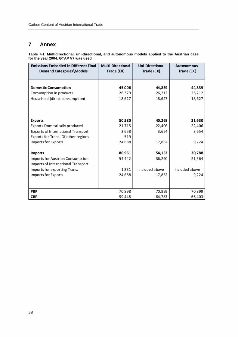
Carbon Content of Austrian International Trade
38
7 Annex
Table 7-1: Multidirectional, uni-directional, and autonomous models applied to the Austrian case for the year 2004. GTAP V7 was used
Emissions Embodied in Different Final Demand Categories\Models
Multi‐Directional Trade (EX)
Uni‐Directional Trade (EX)
Autonomous‐ Trade (EX)
Domestic Consumption 45,006 44,839 44,839 Consumption in products 26,379 26,212 26,212 Household (direct consumption) 18,627 18,627 18,627
Exports 50,580 40,268 31,630 Exports Domestically produced 21,715 22,406 22,406 Exports of International Transport 3,658 3,654 3,654 Exports for Trans. Of other regions 519 Imports for Exports 24,688 17,862 9,224
Imports 80,961 54,152 30,788 Imports for Austrian Consumption 54,442 36,290 21,564 Imports of International TransportImports for exporting Trans. 1,831 included above included aboveImports for Exports 24,688 17,862 9,224
PBP 70,898 70,899 70,899 CBP 99,448 84,783 66,403

B The past and current carbon content of Austrian Trade (Input Output Analysis)
39
Table 7‐2 CO2 flows embodied in Austrian imports per region for the years 1997 and 2004 in
thousands of tons
Ranking Regions \CO2 FlowsThousands of tonnes
% Thousands of tonnes
%
1 Germany 7,580 17.08% 11,294 18.22%2 Former Soviet Union 4,294 9.68% 8,003 12.91%3 China 2,917 6.57% 7,142 11.52%4 Rest of Central European Associates 4,011 9.04% 4,608 7.43%5 United States of America 4,459 10.05% 4,054 6.54%6 Italy 1,794 4.04% 2,651 4.28%7 Rest of Middle East 859 1.94% 2,076 3.35%8 Netherlands 1,067 2.41% 1,598 2.58%9 Poland 3,385 7.63% 1,498 2.42%
10 Rest of South African Customs Union 838 1.89% 1,395 2.25%11 Rest of World 178 0.40% 1,247 2.01%12 India 502 1.13% 1,177 1.90%13 Hungary 1,261 2.84% 997 1.61%14 France 883 1.99% 989 1.60%15 United Kingdom 1,107 2.50% 964 1.56%16 Spain 690 1.56% 914 1.48%17 Thailand 446 1.00% 770 1.24%18 Japan 721 1.62% 749 1.21%19 Rest of North Africa 509 1.15% 730 1.18%20 Turkey 512 1.15% 694 1.12%21 Belgium 631 1.42% 588 0.95%22 Malaysia 319 0.72% 566 0.91%23 Canada 646 1.46% 546 0.88%24 Central America and the Caribbean 188 0.42% 499 0.81%25 Taiwan 272 0.61% 499 0.80%26 Indonesia 280 0.63% 498 0.80%27 Korea 446 1.00% 449 0.72%28 Brazil 88 0.20% 417 0.67%29 Australia 304 0.69% 346 0.56%30 Finland 263 0.59% 327 0.53%31 Rest of Sub‐Saharan Africa 182 0.41% 276 0.45%32 Rest of EFTA 136 0.31% 271 0.44%33 Greece 198 0.45% 251 0.41%34 Switzerland 175 0.39% 241 0.39%35 Ireland 130 0.29% 240 0.39%36 Mexico 212 0.48% 227 0.37%37 Sweden 198 0.45% 200 0.32%38 Vietnam 59 0.13% 192 0.31%39 Argentina 39 0.09% 192 0.31%40 Portugal 165 0.37% 183 0.30%41 Hong Kong 53 0.12% 170 0.27%42 Denmark 271 0.61% 149 0.24%43 Philippines 177 0.40% 133 0.21%44 Singapore 400 0.90% 126 0.20%45 Chile 63 0.14% 125 0.20%46 Rest of South Asia 69 0.15% 114 0.18%47 Venezuela 77 0.17% 114 0.18%48 Morocco 38 0.09% 99 0.16%49 Luxembourg 36 0.08% 74 0.12%50 Colombia 39 0.09% 50 0.08%51 Peru 16 0.04% 42 0.07%52 Rest of Andean Pact 20 0.04% 42 0.07%53 New Zealand 45 0.10% 34 0.05%54 Zimbabwe 26 0.06% 30 0.05%55 Bangladesh 17 0.04% 29 0.05%56 Sri Lanka 32 0.07% 23 0.04%57 Rest of South America 6 0.01% 15 0.02%58 Other Southern Africa 18 0.04% 12 0.02%59 Botswana 2 0.01% 11 0.02%60 Tanzania 3 0.01% 11 0.02%61 Uruguay 9 0.02% 10 0.02%62 Uganda 3 0.01% 6 0.01%63 Mozambique 3 0.01% 5 0.01%64 Zambia 3 0.01% 4 0.01%65 Malawi 1 0.00% 2 0.00%66 Austria ‐ 0.00% ‐ 0.00%
1997 2004

Carbon Content of Austrian International Trade
40
Table 7-3: CO2 flows embodied in Austrian exports per region for the years 1997 and 2004 in thousands of tons
Ranking Regions \CO2 FlowsThousands of tonnes
% Thousands of tonnes
%
1 Germany 4,782 23.35% 6,443 23.38%2 United States of America 2,035 9.94% 2,589 9.39%3 Italy 1,527 7.45% 2,588 9.39%4 United Kingdom 1,097 5.35% 1,531 5.55%5 Rest of Central European Associates 969 4.73% 1,482 5.38%6 France 1,045 5.10% 1,413 5.13%7 Switzerland 740 3.62% 933 3.39%8 Spain 429 2.09% 789 2.86%9 Rest of Middle East 464 2.27% 784 2.84%
10 Former Soviet Union 602 2.94% 702 2.55%11 Netherlands 429 2.09% 620 2.25%12 Japan 859 4.20% 596 2.16%13 China 280 1.37% 588 2.13%14 Hungary 472 2.30% 544 1.97%15 Rest of World 440 2.15% 474 1.72%16 Belgium 300 1.46% 408 1.48%17 Poland 299 1.46% 395 1.43%18 Turkey 196 0.95% 371 1.35%19 Australia 164 0.80% 315 1.14%20 Sweden 234 1.14% 301 1.09%21 Denmark 161 0.78% 225 0.81%22 Greece 137 0.67% 218 0.79%23 India 108 0.52% 212 0.77%24 Canada 255 1.25% 212 0.77%25 Brazil 340 1.66% 192 0.70%26 Rest of Sub‐Saharan Africa 93 0.46% 173 0.63%27 Rest of North Africa 143 0.70% 173 0.63%28 Rest of South African Customs Union 87 0.42% 170 0.62%29 Central America and the Caribbean 54 0.26% 163 0.59%30 Rest of EFTA 161 0.79% 147 0.53%31 Portugal 130 0.64% 140 0.51%32 Korea 172 0.84% 134 0.49%33 Hong Kong 116 0.56% 131 0.48%34 Ireland 61 0.30% 125 0.46%35 Finland 98 0.48% 121 0.44%36 Thailand 110 0.54% 121 0.44%37 Mexico 105 0.51% 106 0.38%38 Singapore 87 0.43% 105 0.38%39 Rest of South Asia 23 0.11% 94 0.34%40 Indonesia 114 0.56% 93 0.34%41 Taiwan 83 0.40% 90 0.33%42 Luxembourg 18 0.09% 77 0.28%43 Malaysia 63 0.31% 58 0.21%44 Argentina 97 0.47% 53 0.19%45 Vietnam 15 0.07% 41 0.15%46 Colombia 35 0.17% 37 0.13%47 Venezuela 34 0.17% 36 0.13%48 Morocco 21 0.10% 35 0.13%49 Philippines 52 0.26% 35 0.13%50 New Zealand 32 0.16% 30 0.11%51 Chile 28 0.14% 29 0.10%52 Peru 16 0.08% 21 0.08%53 Rest of Andean Pact 12 0.06% 19 0.07%54 Sri Lanka 3 0.01% 16 0.06%55 Bangladesh 11 0.06% 16 0.06%56 Rest of South America 4 0.02% 7 0.03%57 Tanzania 5 0.03% 7 0.03%58 Uruguay 8 0.04% 7 0.02%59 Other Southern Africa 6 0.03% 6 0.02%60 Botswana 2 0.01% 5 0.02%61 Zambia 1 0.01% 4 0.02%62 Mozambique 2 0.01% 3 0.01%63 Uganda 4 0.02% 3 0.01%64 Zimbabwe 14 0.07% 2 0.01%65 Malawi 1 0.01% 1 0.00%66 Austria ‐ 0.00% ‐ 0.00%
1997 2004

B The past and current carbon content of Austrian Trade (Input Output Analysis)
41
Table 7-4: CO2 drivers at sectoral level and affected sectors due to domestic and foreign final demand in 2004 Cod. Gtap Regions \CO2 Flows
Th. of t. % Th. of t. % Th. of t. % Th. of t. % Th. of t. % Th. of t. %
1 Paddy rice 0 0.00% 1 0.00% 1 0.00% 0 0.00% 0 0.00% 7 0.01%2 Wheat 33 0.11% 27 0.10% 11 0.02% 74 0.25% 116 0.42% 35 0.06%3 Cereal grains nec 17 0.06% 25 0.09% 30 0.05% 27 0.09% 28 0.10% 49 0.08%4 Vegetables, fruit, nuts 120 0.41% 116 0.42% 386 0.62% 85 0.29% 23 0.08% 176 0.28%5 Oil seeds 4 0.01% 8 0.03% 37 0.06% 4 0.01% 6 0.02% 51 0.08%6 Sugar cane, sugar beet 0 0.00% 2 0.01% 0 0.00% 25 0.09% 9 0.03% 9 0.01%7 Plant‐based fibers 12 0.04% 12 0.04% 97 0.16% 7 0.02% 1 0.00% 44 0.07%8 Crops nec 102 0.35% 54 0.20% 175 0.28% 127 0.44% 57 0.21% 147 0.24%9 Bovine cattle, sheep and goats, horses 13 0.05% 18 0.07% 11 0.02% 45 0.16% 23 0.08% 23 0.04%
10 Animal products nec 45 0.15% 46 0.17% 59 0.09% 76 0.26% 36 0.13% 79 0.13%11 Raw milk 86 0.29% 30 0.11% 63 0.10% 77 0.27% 19 0.07% 27 0.04%12 Wool, silk‐worm cocoons 0 0.00% 3 0.01% 2 0.00% 0 0.00% 0 0.00% 6 0.01%13 Forestry 40 0.14% 14 0.05% 58 0.09% 81 0.28% 94 0.34% 107 0.17%14 Fishing 11 0.04% 20 0.07% 28 0.05% 6 0.02% 1 0.00% 64 0.10%15 Coal 0 0.00% 2 0.01% 7 0.01% ‐ 0.00% ‐ 0.00% 174 0.28%16 Oil 0 0.00% 0 0.00% 0 0.00% 39 0.13% 23 0.08% 671 1.08%17 Gas 0 0.00% 3 0.01% 0 0.00% 0 0.00% 0 0.00% 420 0.68%18 Minerals nec 49 0.17% 7 0.03% 124 0.20% 293 1.01% 206 0.75% 495 0.80%19 Bovine meat products 38 0.13% 110 0.40% 78 0.13% 12 0.04% 11 0.04% 15 0.02%20 Meat products nec 49 0.17% 150 0.54% 229 0.37% 16 0.05% 18 0.07% 30 0.05%21 Vegetable oils and fats 14 0.05% 62 0.22% 99 0.16% 10 0.04% 13 0.05% 33 0.05%22 Dairy products 246 0.84% 312 1.13% 398 0.64% 121 0.41% 62 0.22% 51 0.08%23 Processed rice 1 0.00% 24 0.09% 16 0.03% 1 0.00% 1 0.00% 8 0.01%24 Sugar 41 0.14% 35 0.13% 54 0.09% 39 0.13% 17 0.06% 21 0.03%25 Food products nec 1,420 4.87% 936 3.40% 2,242 3.62% 700 2.40% 205 0.75% 243 0.39%26 Beverages and tobacco products 201 0.69% 407 1.48% 431 0.70% 73 0.25% 79 0.29% 44 0.07%27 Textiles 236 0.81% 296 1.07% 1,331 2.15% 98 0.33% 105 0.38% 335 0.54%28 Wearing apparel 276 0.95% 452 1.64% 1,713 2.76% 45 0.16% 18 0.07% 69 0.11%29 Leather products 95 0.33% 195 0.71% 886 1.43% 21 0.07% 21 0.08% 67 0.11%30 Wood products 121 0.41% 298 1.08% 491 0.79% 82 0.28% 179 0.65% 100 0.16%31 Paper products, publishing 563 1.93% 560 2.03% 840 1.36% 660 2.26% 820 2.98% 628 1.01%32 Petroleum, coal products 246 0.85% 118 0.43% 1,193 1.92% 312 1.07% 187 0.68% 1,678 2.71%33 Chemical, rubber, plastic products 794 2.72% 1,339 4.86% 3,471 5.60% 1,006 3.45% 1,975 7.17% 5,084 8.20%34 Mineral products nec 921 3.16% 389 1.41% 985 1.59% 2,436 8.36% 2,226 8.08% 4,311 6.96%35 Ferrous metals 34 0.12% 176 0.64% 80 0.13% 1,100 3.77% 5,156 18.71% 5,845 9.43%36 Metals nec 7 0.02% 58 0.21% 94 0.15% 42 0.14% 226 0.82% 680 1.10%37 Metal products 264 0.90% 598 2.17% 1,298 2.09% 77 0.26% 108 0.39% 271 0.44%38 Motor vehicles and parts 267 0.92% 2,407 8.73% 4,380 7.07% 75 0.26% 252 0.92% 166 0.27%39 Transport equipment nec 69 0.24% 410 1.49% 876 1.41% 33 0.11% 137 0.50% 72 0.12%40 Electronic equipment 123 0.42% 869 3.15% 3,140 5.06% 12 0.04% 31 0.11% 178 0.29%41 Machinery and equipment nec 691 2.37% 2,829 10.27% 6,028 9.72% 122 0.42% 259 0.94% 476 0.77%42 Manufactures nec 441 1.51% 668 2.43% 2,144 3.46% 16 0.05% 7 0.03% 134 0.22%43 Electricity 4,219 14.47% 947 3.44% 2,086 3.37% 9,272 31.80% 5,825 21.14% 24,743 39.92%44 Gas manufacture, distribution 42 0.14% 20 0.07% 486 0.78% 92 0.31% 53 0.19% 870 1.40%45 Water 2 0.01% 52 0.19% 18 0.03% 4 0.01% 2 0.01% 92 0.15%46 Construction 4,166 14.29% 3,280 11.90% 5,237 8.45% 2,551 8.75% 435 1.58% 68 0.11%47 Trade 1,378 4.73% 1,269 4.60% 2,542 4.10% 590 2.02% 387 1.40% 779 1.26%48 Transport nec 4,370 14.99% 1,287 4.67% 4,204 6.78% 5,295 18.16% 4,158 15.09% 7,503 12.10%49 Water transport 5 0.02% 149 0.54% 44 0.07% 23 0.08% 288 1.04% 667 1.08%50 Air transport 772 2.65% 1,400 5.08% 1,299 2.10% 1,351 4.63% 3,257 11.82% 2,677 4.32%51 Communication 207 0.71% 166 0.60% 563 0.91% 91 0.31% 39 0.14% 70 0.11%52 Financial services nec 32 0.11% 165 0.60% 76 0.12% 22 0.07% 18 0.06% 87 0.14%53 Insurance 118 0.40% 181 0.66% 413 0.67% 7 0.02% 5 0.02% 33 0.05%54 Business services nec 1,272 4.36% 1,149 4.17% 4,263 6.88% 284 0.97% 196 0.71% 871 1.41%55 Recreational and other services 425 1.46% 896 3.25% 1,216 1.96% 161 0.55% 56 0.20% 220 0.36%56 Public Administration, Defense, Education, 4,429 15.19% 2,396 8.70% 5,901 9.52% 1,337 4.59% 84 0.31% 184 0.30%57 Dwellings 27 0.09% 113 0.41% 57 0.09% 0 0.00% 0 0.00% 0 0.00%
Total Sectors 29,153 100% 27,558 100% 61,989 100% 29,153 100% 27,558 100% 61,989 100%
CO2 Emissions Embodied InDomestic
ConsumptionExports Imports
Sectors Affected InAustria by Austrian
Domestic Consumption
Austria by Austrian Exports
Rest of the World by Austrian
Consumption


C Post Kyoto Climate Policies and their impact on Carbon content of Austrian Trade (CGE Analysis)
43
C POST KYOTO CLIMATE POLICIES AND THEIR IMPACT ON CARBON CONTENT OF AUSTRIAN TRADE (COMPUTABLE GENERAL EQUILIBRIUM ANALYSIS)
1 Introduction
We develop a computable general equilibrium (CGE) model to analyze the economic impacts
of carbon dioxide emission constraints taken unilaterally or globally, with a focus on the
(feedback‐) effects via international trade and its respective net carbon flows. For that
purpose, we construct a CGE model for the Austrian economy, its main trading partners
(Germany, Italy, USA, Russia and China), three regional aggregates for the other EU member
states, and 11 larger world regions. On the sectoral level, we differentiate between 11 sectors
according to their energy intensity. The model is originally calibrated to the base year 2004.
Since, however, the climate political targets discussed at the advent of the UNFCCC
Copenhagen meeting are all directed towards the achievement period 2020, our analysis
focuses also on this commitment period. Accordingly, we construct a business as usual (BAU)
scenario for 2020 and compare the impacts of the different policy scenarios to this BAU trend.
In our policy analysis, we discuss three types of scenarios:
- A continuation of a unilateral EU climate policy, analytically differentiated into targets for
the ETS sectors only (as the current EU ETS) and with additional targets for non‐ETS sectors
and households, reflecting the EU 20‐20 targets (European Commission, 2008)
- A voluntary Post‐Kyoto agreement of Annex I countries (characterized by quite weak
emission targets for Russia and the US), at the reduction targets stated before the
UNFCCC’s conference in Copenhagen
- A compulsory global agreement of Annex I countries, with reduction targets as identified
by the IPCC’s 4th Assessment Report to remain within the +2° global temperature target
(compared to pre‐industrial levels) by 2100
For both, the post‐Kyoto and the IPCC scenarios, we distinguish between a ‘high’ and a ‘low’
scenario, since reduction targets have been stated in ranges instead of a single number.
The structure of the remainder of this chapter is as follows. We start by a description of the
data source used for the modeling in section 2. Section 3 describes the structure of the CGE
model, while the assumptions for the policy scenarios and the results for the BAU 2020 are

Carbon Content of Austrian International Trade
44
given in section 4. Section 5 describes the model findings of the different policy scenarios,
namely their impacts for Austria’s output, exports and imports, and their respective carbon
emissions. The economic and carbon effects of the scenarios on a global scale are discussed in
section 5.3, addressing also the problem of carbon leakage due to unilateral policies and the
effectiveness of possible policy reactions, such as the impacts of compensation measures like
the intensively discussed concept of border tax adjustment.

C Post Kyoto Climate Policies and their impact on Carbon content of Austrian Trade (CGE Analysis)
45
2 Data sources for the modeling framework
2.1 Economic and trade data and its sectoral and regional aggregation
The underlying data base for the analysis of the carbon content of Austria’s international trade
is GTAP Version 7 (GTAP, 2007), containing the most recent and consistent input output and
foreign trade accounts for 113 countries and 57 commodities for the base year 2004.
Furthermore the data base provides information on international energy markets derived from
the International Energy Agency’s (IEA) energy volume balances, again for the year 2004
(McDougall and Lee, 2006; McDougall and Aguiar, 2007; Rutherford and Paltsev, 2000). GTAP7
relies on updated energy prices for the year 2004 – using price indices and exchange rates –
from the year 2000, to add information about the monetary energy input values to the
physical energy quantities.
Table 2-1: Overview of regions
Aggregated Region Model code Comprising GTAP regions
Austria AUT Austria
Germany GER Germany
Italy ITA Italy
Rest of West EU 27 + Switzerland WEU Belgium, France, Luxemburg, Netherlands, Portugal,
Spain, Switzerland
Rest of South/-east EU 27 SEEU Cyprus, Czech Republic, Greece, Hungary, Malta, Poland, Slovakia, Slovenia, Bulgaria, Romania
North EU 27 NEU Denmark, Estonia, Finland, Ireland, Latvia, Lithuania, Norway, Sweden, UK
Rest of Europe ROE Rest of EFTA (Liechtenstein, Iceland), Albania, Croatia, Moldova, Rest of Europe (Bosnia and Herzegovina, Gibraltar,…), Turkey
Russian Federation RUS Russian Federation
Rest of GUS GUS Armenia, Azerbaijan, Belarus, Georgia, Kazakhstan, Kyrgyzstan, Rest of former Soviet Union, Ukraine
China CHN China
Rest of East Asia (“Asian Tigers”) EASI Hong Kong, Japan, Korea, Taiwan, Rest of East Asia
Southeast Asia SEASI Cambodia, Indonesia, Lao People’s Democratic Republic, Myanmar, Malaysia, Philippines, Singapore, Thailand, Vietnam, Rest of Southeast Asia
South Asia SASI Bangladesh, India, Pakistan, Sri Lanka, Rest of South Asia
United States of America USA United States of America
Rest of North America NAM Canada, Mexico, Rest of North America
Latin America LAM Argentina, Bolivia, Brazil, Chile, Colombia, Ecuador, Paraguay, Peru, Uruguay, Venezuela, Rest of South America, Costa Rica, Guatemala, Nicaragua,

Carbon Content of Austrian International Trade
46
Panama, Rest of Central America, Caribbean
Oceania OCEA Australia, New Zealand, Rest of Oceania
Middle East and North Africa MENA Egypt, Morocco, Tunisia, Iran, Rest of West Asia, Rest
of North Africa
Sub Saharan Africa SSA
Nigeria, Senegal, Rest of West Africa, Rest of Central Africa, Rest of South Central Africa, Ethiopia, Madagascar, Malawi, Mauritius, Mozambique, Tanzania, Uganda, Zambia, Zimbabwe, Rest of Eastern Africa, Botswana, South Africa, Rest of South African Customs Union
Source: Based on GTAP (2007)
Table 2‐1 gives an overview of the regional aggregation used for the CGE analysis. The regional
(dis)aggregation is based on the importance of individual countries or regions to the climate
policy debate as well as on the basis of an analysis of Austria’s main trading partners – leading
to the selection of Germany (GER), Italy (ITA), Russian Federation (RUS), China (CHN) and the
United States (USA) as single countries modeled separately. The remaining member states of
the European Union 27 were aggregated to West EU27 (WEU), Southeast EU27 (SEEU) and
North EU27 (NEU) in order to be able to carry out an in depth analysis of Austrian trade with
the diverse parts of the EU27. Further aggregates are based on geographical occurrences, their
common role in climate negotiations as well as the affiliation to certain alliances, like the
Commonwealth of Independent States (CIS/GUS).
Table 2-2: Overview of sectors
Aggregated Sectors Model Code Comprising GTAP sectors
Refined oil products P_C Manufacture of coke oven- and refined oil products
Electricity ELY Production, collection and distribution of electricity
Energy intensive industries EIS Chemical industry, non-metallic mineral products, iron and steel, precious and non-ferrous metals, paper products
Non energy intensive industries NEIS
Textiles, wearing apparel, leather, wood products, fabricated metal products, motor vehicles, transport equipment, machinery, communication equipment
Coal COA Coal Mining
Crude Oil OIL Oil extraction
Natural Gas GAS Natural Gas extraction, manufacture of gas, distribution, steam and hot water supply
Transport TRN Water, air, road and rail transport
Food products and agriculture FOOD All agriculture and food processing sectors
Other services and utilities SERV Water, wholesale, retail sale, hotels, restaurant, construction, financial services, insurance, real estate, public administration, post and telecom
Capital Goods CGDS Capital Goods
Source: Based on GTAP (2007)

C Post Kyoto Climate Policies and their impact on Carbon content of Austrian Trade (CGE Analysis)
47
The sectoral aggregation to be used in the CGE model – depicted in Table 2‐2 – was selected
according to energy ‐ and therefore GHG emission – intensity. We distinguish between sectors
with high and with low energy intensity, respectively. Primary energy extraction is reflected in
GTAP by the sectors coal (COA), oil (OIL) and natural gas (GAS), which also incorporates gas,
steam and hot water distribution. Derived energy goods include refined oil and coke oven
products (P_C) and electricity including its distribution (ELY). The industrial sectors within
GTAP7 are split in two groups according to their energy intensities in production. The
aggregate Energy Intensive Sectors (EIS) comprises the industries which are responsible for the
bulk of a country’s production related GHG emissions and its production units are therefore
also subject to the EU’s Emission Trading Scheme (ETS) (European Parliament, 2003). The most
prominent industries within this group are iron and steel, chemicals, cement and paper. The
rest of the industries – i.e. the non‐energy intensive sectors – which are characterized by a
lower CO2 coefficient in their production processes, are merged in the NEIS aggregate.
2.2 Energy and emissions
The remaining crucial data prerequisite for our analysis is the detailed knowledge of emissions
originating from the production processes of various sectors in various countries and regions.
Lee (2008) started a first attempt to generate CO2 emissions data for the GTAP7 database.
Since these CO2 emissions are derived from the IEA energy balances, included in GTAP7, they
only take account of combustion based CO2 emissions. This data therefore is excluding some
10% of global CO2 emissions which are triggered by industrial processes. While 10% might
seem negligible, it is not in our context of analysis, because it is 10% of global emissions
originating from basically three economic sectors (iron and steel, cement, oil refinement) that
each are foreign trade intensive and under fierce international competition. We cannot accept
to misrepresent the carbon content of these carbon intensive sectors and their trade flows, a
misrepresentation that for iron and steel for example can easily concern more than 50% of
sectoral CO2 emissions. While GTAP7 and all international studies based on this data base only
do neglect process emissions, we thus had to incorporate these process related emissions in a
separate step, thereby relying on UNFCCC data (UNFCCC, 2009). These GHG emissions from
industrial processes mainly occur in the cement, chemicals and metal production and are
therefore added to the EIS aggregate’s emissions balance. Another flaw of Lee’s CO2 emissions
calculation lies in the misinterpreted treatment – at least for Austria – of fuels used as
feedstock in the chemical and petrochemical industry (P_C). This leads to an underestimation

Carbon Content of Austrian International Trade
48
of these industries’ CO2 emissions compared to more detailed data for Austria
(Umweltbundesamt, 2008). Based on this additional information and on our own work in this
field (Steininger et al., 2009), a reconciliation of the Austrian CO2 data is possible in principle.
However, since we have detailed knowledge at this level of detail of CO2 emissions only for
Austria, unilateral data reconciliation would artificially worsen Austria’s P_C and chemical
sectors’ international competitiveness in a stricter EU climate policy scenario. To keep global
consistency within the GTAP7 data set and to avoid implausible model results at the expense
of Austrian industrial sectors, we thus stick to the initial CO2 data base by Lee, but augmented
by industrial process related emissions, yet without correction for feedstock use in these
sectors.
2.3 Economic dynamics
In our CGE analysis, we examine Austria’s international trade and its net carbon flows for the
time horizon 2020. The year 2020 was chosen because it reflects the time frame for the EU’s
proposed 2020 targets – a 20% reduction of GHG emissions below 1990 levels (‐30% if there is
an international mitigation agreement negotiated with other developed countries) and a 20%
share of renewable energies in EU energy consumption until 2020 (European Commission,
2008). Also, many other officially announced reduction strategies by single countries, regions
or by the IPCC (IPCC, 2007) refer to the year 2020.
Since the GTAP7 data base is consistent for the reference year 2004 and we apply a static
general equilibrium model calibrated for this base year, we have to factor in the economic
developments until the year 2020 by growth rates. In Poncet (2006) a comprehensive study of
the long term growth prospects of the world economy was carried out, providing annual
average growth rates for the time span 2005 to 2050 for multi‐factor‐productivity (MFP), the
capital stock and the labor force. To account for improvements in energy efficiency over time,
we introduce an exogenous autonomous energy efficiency improvement parameter AEEI. The
AEEI is a heuristic measure for all non‐price driven improvements in technology, which in turn
reduces energy intensity. Following Böhringer (1999) and Burniaux et al. (1992) we assume a
constant AEEI parameter and set it to 1% per annum. Table 2‐3 gives an overview of the
growth rates which were used to calculate our model for the 2020 Business As Usual (BAU)
scenario.

C Post Kyoto Climate Policies and their impact on Carbon content of Austrian Trade (CGE Analysis)
49
Table 2-3: Annual Growth rates 2004 – 2020
Regions MFP* Capital stock* labor force*
AUT 1.30 1.40 -0.20
GER 1.50 1.60 -0.10
ITA 1.30 1.10 -0.50
WEU 1.40 1.60 -0.03
SEEU 1.40 2.00 -0.40
NEU 1.40 2.50 0.20
ROE 1.50 1.80 0.30
RUS 1.50 1.80 0.30
GUS 1.50 1.80 0.30
CHN 2.60 5.70 0.10
EASI 1.50 2.20 -0.30
SEAS 2.70 5.20 0.60
SASI 2.10 4.40 0.80
USA 1.50 2.60 0.70
NAM 1.60 2.60 0.50
LAM 0.50 1.40 0.70
OCEA 1.60 3.00 0.50
MENA 0.90 1.10 1.00
SSA 0.50 0.90 0.50
*based on Poncet (2006) **based on IMF (2009)

Carbon Content of Austrian International Trade
50
3 The model
For our analysis of the carbon content of Austria’s international trade in the presence of
climate policies, we employ a large‐scale multiregional, multisectoral computable general
equilibrium model (CGE), programmed and solved in GAMS/MPSGE (Rutherford, 1999) utilizing
the solver PATH, which is calibrated to the previously described GTAP7 data base, representing
the year 2004. As illustrated in the previous section, we differentiate for 19 world
regions/countries and 11 sectors. The remainder of this chapter gives a detailed description of
the CGE model structure, which follows in its basic structure the GTAP‐E model, as well as the
parameters applied for the evaluation of different policy scenarios (see chapter 4).
3.1 Basic model structure
Following the structure of agents used in the social accounting matrix generated by GTAP, the
so‐called regional household RegHHr represents total final demand in each of the 19 regions.
This regional household provides the primary factors capital Kr, labor Lr and natural resources
Rr (primary energy commodities) for the 11 sectors, and receives total income including
various tax revenues. The regional household redistributes this stream of income between the
private household PHHr and the government GOVr for private and public consumption,
respectively. We model capital and labor as mobile between sectors within a region, but
immobile among different regions. Moreover, again following the structure of the GTAP social
accounting matrix, a specific resource input is used in the production of crude oil, natural gas
and coal; therefore those three sectors represent the extraction of primary energy. Thus, there
are two different groups of production activities which are represented by slightly different
production functions in the model: the production of non‐primary energy commodities, and
primary energy extraction. The following section provides a description of the production
function modeling approach, while the subsequent section deals with modeling trade, taking
the form of bilateral trade relationships rather than an integrated global market.
3.2 Production structure
Within the modeling framework MPSGE, nested constant elasticity of substitution (CES)
production functions are employed, to specify the substitution possibilities in domestic
production between the primary inputs (capital, labor, and natural resources), intermediate
energy and non‐energy inputs as well as substitutability between energy commodities

C Post Kyoto Climate Policies and their impact on Carbon content of Austrian Trade (CGE Analysis)
51
(primary and secondary). There are two groups of produced commodities – primary energy
and non‐primary energy commodities. Figure 3‐1 illustrates the structure of the production of
primary energy commodities (PrimNrg). At the top level in the extraction of fossil resources,
natural resources and non resource inputs can be exchanged with a constant elasticity of
substitution s, equaling to zero, which characterizes a Leontief composite.
Figure 3-1: Nesting structure of primary energy extraction
At the second level, the Armington aggregation of domestic and imported intermediate inputs
– the domestic supply Desc,r – from non‐energy sectors are employed in fixed proportions v
with an aggregate of capital, labor and energy ((KL)Er). At the third nesting level, a CES
composite of capital and labor (KLr) is combined in fixed proportions (elke) with an energy‐
composite. The energy‐composite Er consists of three main nesting stages. The first one
represents a trade off at a constant elasticity elc between the domestic supplied secondary
energy commodities electricity (ELY) DELY,r and petroleum products (P_C) PC/CO2 r with an
aggregate of primary energy commodities (OIL/GAS/COAr). At the subsequent level this
primary energy‐composite is comprised of a CES function (elcl) between the domestic supply
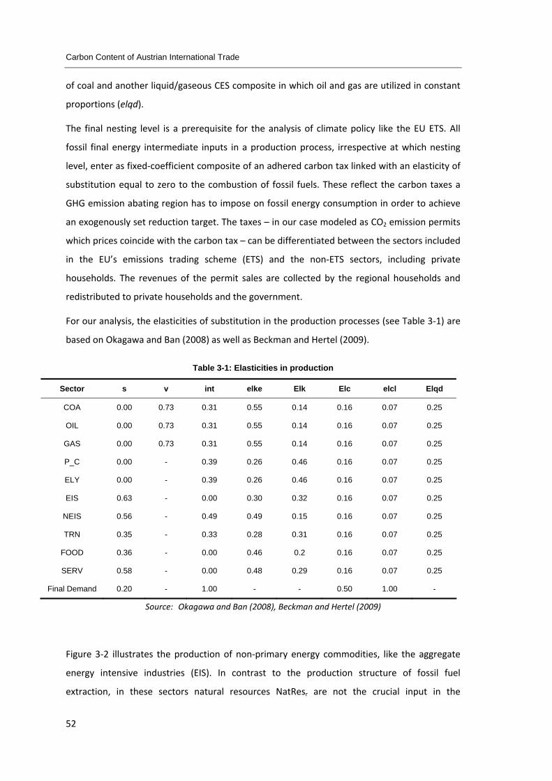
Carbon Content of Austrian International Trade
52
of coal and another liquid/gaseous CES composite in which oil and gas are utilized in constant
proportions (elqd).
The final nesting level is a prerequisite for the analysis of climate policy like the EU ETS. All
fossil final energy intermediate inputs in a production process, irrespective at which nesting
level, enter as fixed‐coefficient composite of an adhered carbon tax linked with an elasticity of
substitution equal to zero to the combustion of fossil fuels. These reflect the carbon taxes a
GHG emission abating region has to impose on fossil energy consumption in order to achieve
an exogenously set reduction target. The taxes – in our case modeled as CO2 emission permits
which prices coincide with the carbon tax – can be differentiated between the sectors included
in the EU’s emissions trading scheme (ETS) and the non‐ETS sectors, including private
households. The revenues of the permit sales are collected by the regional households and
redistributed to private households and the government.
For our analysis, the elasticities of substitution in the production processes (see Table 3‐1) are
based on Okagawa and Ban (2008) as well as Beckman and Hertel (2009).
Table 3-1: Elasticities in production
Sector s v int elke Elk Elc elcl Elqd
COA 0.00 0.73 0.31 0.55 0.14 0.16 0.07 0.25
OIL 0.00 0.73 0.31 0.55 0.14 0.16 0.07 0.25
GAS 0.00 0.73 0.31 0.55 0.14 0.16 0.07 0.25
P_C 0.00 - 0.39 0.26 0.46 0.16 0.07 0.25
ELY 0.00 - 0.39 0.26 0.46 0.16 0.07 0.25
EIS 0.63 - 0.00 0.30 0.32 0.16 0.07 0.25
NEIS 0.56 - 0.49 0.49 0.15 0.16 0.07 0.25
TRN 0.35 - 0.33 0.28 0.31 0.16 0.07 0.25
FOOD 0.36 - 0.00 0.46 0.2 0.16 0.07 0.25
SERV 0.58 - 0.00 0.48 0.29 0.16 0.07 0.25
Final Demand 0.20 - 1.00 - - 0.50 1.00 -
Source: Okagawa and Ban (2008), Beckman and Hertel (2009)
Figure 3‐2 illustrates the production of non‐primary energy commodities, like the aggregate
energy intensive industries (EIS). In contrast to the production structure of fossil fuel
extraction, in these sectors natural resources NatResr are not the crucial input in the

C Post Kyoto Climate Policies and their impact on Carbon content of Austrian Trade (CGE Analysis)
53
production process, with the exception of some agricultural activities (incorporated in the
FOOD aggregate) using resources as direct intermediate inputs. Accordingly, the top level CES
function between natural resources and non‐resource inputs is replaced by the originally
second nesting level – the constant tradeoff between domestically supplied non‐energy
intermediate inputs Desc,r and a capital‐labor‐energy aggregate((KL)Er). The natural resource
input NatResr (only relevant for FOOD sector production) is moved to the third nesting level,
where it is employed in fixed proportion with a capital‐labor‐natural resource composite at an
elasticity elk. Unique in the EIS sector is the inclusion of CO2 emissions related with industrial
processes ProcessCO2 r, which are nested in a Leontief style CES function together with the
intermediate energy input composite Er.
Figure 3-2: Production of non-primary energy commodities
3.3 Trade in the model
A common assumption within multi‐country CGE models which we also employ here is that
goods produced in different regions are not perfectly substitutable. Therefore, trade in goods

Carbon Content of Austrian International Trade
54
is described by bilateral trade relationships rather than by an integrated global market
(Armington, 1969). An Armington aggregation activity Ges,r, depicted in Figure 3‐3, corresponds
to a CES composite (tela) of domestic Xes,r and imported goods IMes,s,r as imperfect substitutes.
Figure 3-3: Armington aggregation for country r
The associated Armington elasticities (telaes), different in each sector, are presented in Table
3‐2. The resulting Armington supply Ges,r either enters the domestic supply Des,r , satisfying final
demand and intermediate demand in production activities, or is exported to other regions
EXes,s,r , entering again as an imperfect substitute into the formation of the trading partner’s
Armington supply.
Table 3-2: Armington elasticities (telaes)
Sector Armington Elasticity
COA 3.05
OIL 5.20
GAS 10.76
P_C 2.10
ELY 2.80
EIS 3.21
NEIS 3.71
TRN 1.90
FOOD 2.39
SERV 1.91
Source: GTAP (2007)

C Post Kyoto Climate Policies and their impact on Carbon content of Austrian Trade (CGE Analysis)
55
Every bilateral trade flow is linked to a distance dependent amount of transport service Trans
– which is supplied by a global transport sector – by means of a Leontief production function
with an elasticity of substitution equal to zero (see Figure 3‐4). The imports of any particular
region IMes,s consist of imports from either the European Union or the Rest of the World
(ROW), which are traded off at the top level of the import production block amongst each
other at a constant proportion (elim).
Figure 3-4: Import structure for country r
The international transport service activity is assumed to be a Cobb‐Douglas composite of
transport goods TRANSr provided as an aggregate of water, air and land transport domestic
market activities (TRN) by each region (see Figure 3‐5). This global market thereupon delivers
the transport services required for imports to the individual regions.
Figure 3-5: International Transport

Carbon Content of Austrian International Trade
56
The parameters m and n depict the constant elasticity of substitution between EU regions and
ROW regions respectively (Figure 3‐4). Values for these elasticities applied in the modeling of
imports are presented in Table 3‐3.
Table 3-3: Elasticities in import structure
Elasticity value
elim 8
m 4
n 4
rg 4
Source: Rutherford and Paltsev (2000)
3.4 Final demand
Final Demand in each region is determined by consumption of the private household and the
government. Both the private household and the government maximize utility subject to their
disposable income received from the regional household. Disposable income is composed of
all factor income and tax revenues. Following the GTAP structure, we differentiate for a broad
range of direct taxes (on capital, labor and resource inputs), indirect taxes (intermediate taxes,
production taxes or subsidies, consumption taxes, export taxes or subsidies and import tariffs),
and we add environmental levies in the form of CO2 permits.
Figure 3-6: Final demand of private households for country r

C Post Kyoto Climate Policies and their impact on Carbon content of Austrian Trade (CGE Analysis)
57
Consumption of private households in each region, depicted in Figure 3‐6, is characterized by a
constant elasticity aggregate of a non‐energy intermediate consumption bundle Des,r and an
energy aggregate Er (elasticity: s). The energy composite itself consists again of two nesting
levels – a CES function with an elasticity elc, trading off secondary energy (ELY and P_C) with a
primary energy fixed proportion composite (elk). The combustion of fossil fuels in the private
households in each country is linked in the same way to CO2 taxes as it is the case in the
production of energy and non‐energy commodities.
Having described the structure of the CGE model, and before using the model to analyze
different climate policy scenarios, the following section will outline the settings of three
different scenario families – a unilateral EU scenario group, a post‐Kyoto agreement with a
voluntary commitment by other countries in addition to the EU, as well as the spectrum of the
IPCC’s recommendation on GHG emission reductions for Annex I countries to the Kyoto
Protocol.
Carbon Content of Austrian International Trade
58
4 Definition of policy scenarios
4.1 Post-Kyoto climate policies
Table 4‐1 presents five different 2020 policy scenarios which are evaluated by means of our
CGE model. The first two scenarios, ETS_EU and NETS_EU, refer to unilateral EU policies as set
up by the EU20‐20 objectives: under ETS_EU a 21% reduction target relative to 2005 CO2
emission levels is implemented in all sectors which are included in the current EU ETS, namely
the energy intensive industries (EIS), the power generation sector (ELY), and the petrochemical
industry (P_C). In the NETS_EU setting, an additional 10% reduction target is introduced in the
non energy intensive industries and for private households, again 2020 emission levels
compared to 2005 emission levels. In both scenarios, the policies are implemented EU wide.
For the ETS sectors we allow for an emission trading scheme with emission permits traded
among all EU countries (leading to a common carbon price across Europe for these sectors).
For the non‐ETS sectors and the private households we do have national targets implying a
national shadow price of carbon emission in these sectors that differs across countries.
The remaining scenarios cover global policies with other world regions setting reduction
objectives as well, albeit at different stringency levels. The two global post‐Kyoto scenarios
PK_L and PK_H presume that CO2 emission reduction targets have been set voluntarily by
many industrialized countries within a global agreement established at the upcoming
Copenhagen Conference of the UNFCCC. The reduction targets depicted in Table 4‐1 refer to
the most recent, official country specific information (L is the lower and H the higher bound)
on envisioned GHG reduction goals, relative to emissions in the base year 1990. Since there
are no specific reduction targets announced for the specific regional aggregation adopted
within this paper, we generated reduction objectives for the respective regions by aggregating
the available country targets and emissions. For instance, the ‐8% CO2 reduction goal for the
rest of GUS results since only Belarus and the Ukraine have officially announced CO2 objectives
of ‐5% and ‐20%, respectively in a low reduction scenario (‐10% and ‐20% for a high abatement
scenario) prior to the Copenhagen climate talks, while emissions in all other GUS countries are
allowed to grow without restrictions.

C Post Kyoto Climate Policies and their impact on Carbon content of Austrian Trade (CGE Analysis)
59
Table 4-1: GHG emission reduction targets for 2020
Region Unilateral EU Climate Policy Voluntary post-Kyoto agreement IPCC requirements 450ppm
ETS_EU NETS_EU PK_L PK_H IPCC_L IPCC_H
base year 2005 2005 1990 1990 1990 1990
EU -21% in ETS sectors
-21% in ETS sectors, -10% in non-ETS sectors+ households
-20% in all sectors and households
-30% -25% -40%
RUS -10% -15% -25% -40%
ROE +52% +51% -17% -28%
GUS -8% -8% -11% -18%
USA +/-0% -4% -25% -40%
NAM -3% -3% -14% -23%
LAM
CHN
EASI -25% -25% -15% -23%
SEASI
SASI
OCEA +10% -11% -25% -40%
MENA
SSA
Source: European Commission (2008); IPCC (2007); personal communication Andreas Tuerk (2009)
While the post‐Kyoto scenarios are the result of voluntary emission reduction targets by Annex
I countries, the remaining two IPCC scenarios are based on the recommended ‐25% to ‐40%
GHG emission cuts in all Annex I countries which are necessary to remain within the crucial
+2C° target by 2100 compared to preindustrial periods (IPCC, 2007). While the IPCC
acknowledges that a major deviation from baseline emissions will be necessary also within
non‐Annex I countries, no specific, official reduction targets have been communicated yet. As a
consequence, reduction targets of non‐Annex I countries will not be considered in the
subsequent analysis. As for the post‐Kyoto scenarios, emissions reduction objectives for
country groups are determined by weighing the reduction targets for Annex I with the base
year emissions for both Annex I and non‐Annex I countries within the respective regions.
In order to implement the officially announced GHG emission reduction objectives depicted in
Table 4‐1 in our model, we recalculate the emission targets relative to the base year 2004 (see
Table 4‐2). Depending on the development of the regions’ CO2 emissions relative to the
scenarios’ respective base years (2005 for ETS_EU and NETS_EU, all other scenarios 1990),

Carbon Content of Austrian International Trade
60
these reduction targets deviate in some cases substantially from the ones presented in Table
4‐1. For example the reduction goal in the ETS_EU scenario, which was a homogenous ‐21%
reduction for all EU member states, slightly changed by country according to the changes in
observed CO2 emissions between 2004 and 2005, resulting in regional diversified targets for
the base year 2004.
Table 4-2: GHG emission reduction targets for 2020 relative to 2004
Region ETS_EU NETS_EU PK_L PK_H IPCC_L IPCC_H
sectors ETS ETS+NETS ETS+NETS ETS+NETS ETS+NETS ETS+NETS
AUT -20% -14% -36% -44% -40% -52%
GER -24% -17% -6% -18% -12% -29
ITA -21% -13% -29% -38% -33% -47%
WEU -20% -11% -35% -43% -39% -51%
SEEU -21% +11% -7% -19% -13% -30%
NEU -23% -17% -20% -30% -25% -40%
RUS +48% +39% +23% -2%
ROE +4% +3% -44% -51%
GUS +22% +22% +18% +9%
USA -16% -19% -37% -50%
NAM -16% -3% -26% -34%
LAM
CHN
EASI -30% -30% -20% -28%
SEASI
SASI
OCEA -18% -11% -44% -55%
MENA
SSA
By comparing the reduction targets in Table 4‐1 and Table 4‐2, crucial information can be
attained from the comparison of Russia’s reduction goals. Russia’s officially announced
reduction target in a post‐Kyoto agreement would amount to a 15% reduction vis a vis 1990
emissions in a high scenario. By changing the reference year from 1990 to 2004, the target
changes from a reduction requirement to an increase in CO2 emissions since Russia’s 1990 CO2
emissions were substantially higher than in 2004. Only in the strongest IPCC scenario –
representing a 40% reduction of GHG in Annex I countries – Russia would be confronted with a
minor effective reduction objective of 2% compared to 2004 CO2emissions. The same rationale
holds for the rest of the GUS region, while one can see the rise in the ROE region’s CO2

C Post Kyoto Climate Policies and their impact on Carbon content of Austrian Trade (CGE Analysis)
61
emissions reflected in the more stringent reduction target compared to the base year 2004
instead of 1990.
4.2 The BAU 2020 scenario
In the subsequent analysis all results will be compared to a business as usual scenario (BAU)
for 2020, since this is the period for which both at the UNFCCC and European level reduction
targets are negotiated. To develop the BAU scenario for 2020, we combine the economic data
for 2004 with data on growth in multifactor productivity, labor force and capital stock
discussed in section 2.3. By applying these (exogenous) annual growth rates to the model,
which was initially calibrated for the GTAP7 base year 2004, we develop an economic structure
for the year 2020 – representing a possible future scenario based on 2009 knowledge about
future economic growth in presence of the ongoing economic crises. Considering the current
economic downturn, we decided to apply the annual growth rates by Poncet (2006), which
were calculated prior to the advent of the financial crises, not for the whole 16 year time
differential between 2004 and 2020, but only for a reduced ten year time span. This procedure
should counterbalance the setbacks in growth prevailing in 2008 and 2009 and which will not –
again based on the most recent information by EUROSTAT and others – come to a halt earlier
than 2011.
This adjustment procedure allows us to generate a BAU scenario for the year 2020, which will
be used as a benchmark in our analysis of the consequences of climate policies for the Austrian
economy, especially focusing on the (changing) carbon content of Austria’s international trade
relationships. To get a better understanding of this benchmark by introducing the ‘crises
adjusted’ growth prospects, let us look at a few numbers. The scenario is characterized by an
average annual GDP growth rate of 2.2% for Austria (over the period 2004 to 2020), resulting
in a GDP of 413.3 billion USD in 2020 (due to the GTAP database, all GDP data is presented in
USD, at 2004 real prices). In comparison, the average annual GDP growth rate in Austria for the
time period 1999 to 2008 – therefore before the economic downswing – was 2.4% (see Table
2‐3).

Carbon Content of Austrian International Trade
62
Table 4-3: BAU 2020 scenario for Austria (in million USD, below: MUSD)
2004 2020 % change 2020
relative to 2004 in MUSD (real at 2004 prices) in % GDP
Consumption 172,494 247,414 +43% Investment 67,168 101,964 +52% Government 54,933 78,793 +43% Trade balance -2,283 -14,843 +550%
Total 292,312 413,328 +41% annual average growth rate 2.41 2.19 Output
P_C 3,689 4,363 +18% ELY 6,557 7,617 +16% EIS 58,932 71,641 +22%
ETS total 69,179 83,621 +21% COA 27 31 +14% OIL 267 304 +14% GAS 298 340 +14% NEIS 118,850 147,779 +24% TRN 38,328 50,380 +31% FOOD 30,617 41,402 +35% SERV 279,362 360,201 +29% CGDS 67,168 101,964 +52%
non-ETS total 534,918 702,401 +31% Output total 604,097 786,022 +30% Export
P_C 274 334 +22% ELY 786 890 +13% EIS 26,285 32,461 +23%
ETS total 27,345 33,684 +23% COA 0 0 +28% OIL 0 0 +85% GAS 30 36 +19% NEIS 61,503 77,146 +25% TRN 10,481 13,642 +30% FOOD 6,309 8,634 +37% SERV 29,941 38,231 +28%
non-ETS total 108,265 137,689 +27% Export TRANS 7,061 10,343 +46%
Export total 142,670 181,716 +27%

C Post Kyoto Climate Policies and their impact on Carbon content of Austrian Trade (CGE Analysis)
63
Table 4-4 (cont.): BAU 2020 scenario for Austria (in million USD, below: MUSD)
2004 2020 % change 2020
relative to 2004 in MUSD (real at 2004 prices) in % Import
P_C 2,128 2,560 +20% ELY 1,030 1,400 +36% EIS 24,891 32,694 +31%
ETS total 28,049 36,654 +31% COA 228 238 +4% OIL 1,839 1,932 +5% GAS 859 932 +9% NEIS 63,443 88,673 +40% TRN 5,729 7,635 +33% FOOD 7,684 11,016 +43% SERV 34,445 45,824 +33%
non-ETS total 114,226 156,249 +37% Import TMG 2,678 3,656 +36%
Import total 144,953 196,558 +36%
Under BAU assumptions, the total output of Austria’s economy grows by a total of 30% over
these 16 years. Comparing ETS sectors (ELY, EIS, P_C) with the rest of the economy – the NETS
sectors –, we see that the rise in output is mainly induced by an increase in the NETS sectors by
31%, compared to +21% in the ETS sectors. Since the NETS output volume already in 2004 is
almost eight times the level of that of the ETS output, the increase of the NETS output in
absolute terms is considerably higher than that of the ETS output. Table 4‐3, which presents
the effects of the transition from 2004 to 2020 under the previously illustrated BAU growth
assumptions, gives further insights for the composition of Austrian trade in the years 2004 and
2020. Austria – being a net importer already in the base year 2004 – worsens its trade balance
until the year 2020 by some 13 MUSD. This arises from import volumes increasing relatively
stronger than Austria’s export volumes. For both exports and imports, trade in NETS (especially
the NEIS and SERV aggregates) is much larger in quantitative terms than in ETS. Moreover,
trade in NETS sectors grows slightly more than in ETS sectors.
Table 4‐5 focuses on Austrian trade flows in the BAU‐2020 scenario, distinguishing ETS and
non‐ETS sectors. The first two columns give a detailed account of Austria’s imports from the
other 18 model regions, while the third and fourth columns analyze Austria’s export structure.
Clear evidence is that Austria’s main trading partners, both in 2020 imports and exports, are
found within the EU, in particular the neighboring countries Germany and Italy. The USA and
Russia are its strongest single country trading partners outside the EU. The USA is particularly

Carbon Content of Austrian International Trade
64
important as an export market, while China is the source of NETS imports worth 5.3 billion
USD.
Table 4-5: Austrian trade flows in the BAU 2020 scenario (in MUSD)
Imports 2020 (MUSD) Exports 2020 (MUSD) ETS NETS ETS NETS
GER 17,172 53,784 8,434 38,299 ITA 2,791 13,983 3,139 11,915 WEU 6,644 21,162 6,117 19,840 SEEU 3,685 15,157 6,232 17,035 NEU 3,084 11,036 2,332 11,971 ROE 432 2,551 1,159 4,210 RUS 347 2,053 436 1,680 GUS 158 1,019 289 1,235 CHN 263 5,331 270 2,903 EASI 468 7,872 693 2,831 SEAS 314 5,884 333 3,459 SASI 40 1,068 174 1,845 USA 691 7,253 1,855 10,365 NAM (excl. USA) 97 1,266 391 1,517 LAM 169 1,934 358 1,929 OCEA 38 441 197 1,253 MENA 104 3,317 1,071 3,804 SSA 156 1,136 206 1,597 Total 36,654 156,249 33,684 137,689
4.3 CO2 emissions in the BAU 2020 scenario
Turning to CO2 emissions, Austria’s CO2 emissions under the BAU assumptions are found to
increase of 14.8% compared to 2004, calculated according to the Production Based Principle
(PBP) and thus based on emissions from domestic production. This increase of 14.8%
corresponds to an absolute increase in Austria’s production related and private household’s
emission by 12 Mt CO2 from 79 Mt CO2 in 2004 to 91 Mt CO2 in 2020 (Table 4‐6).
Table 4-6: CO2 emissions for Austria according to the PBP and CBP for 2004 and BAU-2020
2004 2020 % Change in Mt CO2 2004-2020
PrivHH 18.63 23.34 +25.3%
Output 60.42 67.43 +11.6%
PBP 79.05 90.77 +14.8%
Import 27.27 31.25 +14.6%
Export 19.31 22.09 +14.4%
IM-EX 7.96 9.16 +15.1%
CBP 87.01 99.93 +14.9%

C Post Kyoto Climate Policies and their impact on Carbon content of Austrian Trade (CGE Analysis)
65
Following Peters and Hertwich (2008), we move beyond the production based emission
inventory – representing domestic emissions from economic production within a country and
the emissions due to the combustion of fossil fuels in the private sector – to the broader
concept of a consumption based emission inventory. This Consumption Based Principle (CBP)
can ‘be considered a trade‐adjusted version of the production based inventory’ (Peters and
Hertwich, 2008), therefore representing the entity of a country’s CO2 emissions occurring from
its economic consumption. Applying this CBP concept to Austria’s CO2 emissions, we find
emissions to be 87 MT CO2 in 2004 and to rise to 100 Mt CO2 in 2020 (Table 4‐6and Figure 4‐1),
and thus to be considerably higher than emissions according to the PBP. Thus, taking account
of all emissions which are necessary to fulfill Austrian consumption (i.e. final demand), by
adding emissions from imports and subtracting emissions attributed to exports, leads to a
higher amount of carbon emissions according to the CBP than the PBP. This is a typical pattern
which is found for the lion’s share of industrialized countries, while developing countries in
general have a reverse pattern (for a country comparison, see Peters and Hertwich, 2008).
By comparing the increase in emissions from 2004 to 2020, we see an increase in emissions
according to the PBP by 14.8% while emissions according to the CBP increase by 14.9%.
Compared to 2004 output related CO2 emissions increase by 12%, household’s emissions by
25% and emissions embodied in Austria’s net carbon trade flow increase by 15% (Table 4‐6).
However, when the development of Austria’s net carbon trade flows are compared to the
development of its trade balance in monetary terms, one interesting finding arises: While
Austria’s trade deficit increases almost sixfold, its counterpart in terms of CO2 emissions
increases only by 15%. This reflects on the one hand a global increase in energy efficiency in all
production processes and on the other a shift in the composition of imports from carbon
intensive goods (EIS sectors) to low‐carbon products (NEIS and SERV sectors).
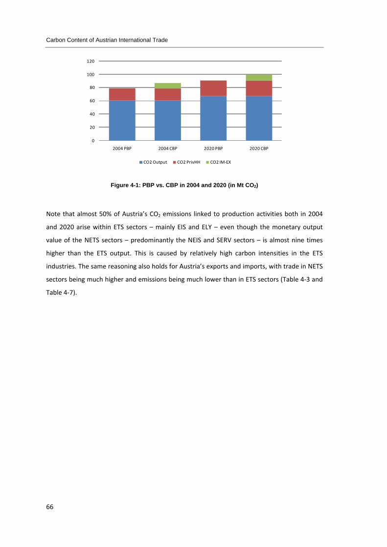
Carbon Content of Austrian International Trade
66
0
20
40
60
80
100
120
2004 PBP 2004 CBP 2020 PBP 2020 CBP
CO2 Output CO2 PrivHH CO2 IM‐EX
Figure 4-1: PBP vs. CBP in 2004 and 2020 (in Mt CO2)
Note that almost 50% of Austria’s CO2 emissions linked to production activities both in 2004
and 2020 arise within ETS sectors – mainly EIS and ELY – even though the monetary output
value of the NETS sectors – predominantly the NEIS and SERV sectors – is almost nine times
higher than the ETS output. This is caused by relatively high carbon intensities in the ETS
industries. The same reasoning also holds for Austria’s exports and imports, with trade in NETS
sectors being much higher and emissions being much lower than in ETS sectors (Table 4‐3 and
Table 4‐7).

C Post Kyoto Climate Policies and their impact on Carbon content of Austrian Trade (CGE Analysis)
67
Table 4-7: BAU-2020 scenario – Sectoral CO2 emissions for output, exports and imports for Austria (in Mt CO2)
2004 2020 % Change in Mt CO2 2004-2020 Private
Households 18.63 23.34 +25% Output
P_C 0.54 0.58 +6% ELY 15.33 16.18 +5% EIS 15.24 15.67 +3%
ETS total 31.12 32.42 +4% COA 0.00 0.00 +0% OIL 0.07 0.06 -7% GAS 0.15 0.15 +3% NEIS 2.22 2.43 +9% TRN 18.10 21.70 +20% FOOD 2.44 3.04 +25% SERV 6.33 7.63 +21% CGDS 0.00 0.00 +0%
non-ETS total 29.30 35.01 +19% Output total 60.42 67.43 +12% Export
P_C 0.04 0.04 +10% ELY 1.84 1.89 +3% EIS 6.80 7.10 +4%
ETS total 8.68 9.03 +4% COA 0.00 0.00 +0% OIL 0.00 0.00 +51% GAS 0.01 0.02 +7% NEIS 1.15 1.27 +10% TRN 4.95 5.88 +19% FOOD 0.50 0.63 +26% SERV 0.68 0.81 +19%
non-ETS total 7.29 8.60 +18% Export TRANS 3.33 4.46 +34% Export total 19.31 22.09 +14% Import
P_C 0.20 0.21 +5% ELY 4.72 5.60 +19% EIS 8.90 9.94 +12%
ETS total 13.82 15.75 +14% COA 0.05 0.05 -5% OIL 0.26 0.23 -11% GAS 1.45 0.81 -44% NEIS 1.61 2.02 +25% TRN 6.12 7.44 +22% FOOD 0.61 0.79 +29% SERV 0.96 1.23 +28%
non-ETS total 11.06 12.56 +14% Import TMG 2.39 2.93 +23% Import total 27.27 31.25 +15%

Carbon Content of Austrian International Trade
68
A fraction of Austria’s imports and exports consists of trade services – air, water and land
based – which are causally linked to import and export activities and which are responsible for
a certain amount of emissions, determined by the transport technology used by the transport
arranging trade partner. As was explained earlier (see section 3), in our modeling framework
each region exports a certain amount of transport services (TRANS) to a global transport
market, which further redistributes the transport services as Import Trade Margins (TMG)
linked to imports. Since within the GTAP database these trade services are attributed in total
and not for each sector separately, the final entries within exports and imports are TRANS and
TMG respectively (see Table 4‐7). Within this globally balanced transport market, Austria is –
based on the GTAP7 database – a net exporter of transport services and its respective CO2
emissions.
5 The economic and global carbon effects of climate policy for Austria as an internationally trading economy
5.1 The economic effects of the climate policy scenarios for Austria
Table 5‐1 summarizes the economic effects of the different climate policy scenarios for Austria
relative to the business as usual (BAU) scenario for the year 2020. In scenario ETS_EU, the
European Union implements an emissions trading scheme in the energy intensive sectors (ETS
sectors, namely P_C, ELY, EIS) only, but the other countries do not limit their emissions. This
leads to a reduction in Austrian GDP by 0.4% relative to BAU, and to a reduction in annual
economic growth from 2.19 in BAU to 2.16. Austrian exports and imports decline by 1.1% and
0.9% respectively. When the European Union extends its climate policy also to the non‐ETS
sectors (as in the NETS_EU scenario; this separation is only done for analytical reasons, as the
EU has a single climate policy focusing on both ETS and NETS) but the other countries still do
not reduce their emissions, effects on GDP, exports and imports are more than doubled. The
post Kyoto scenarios PK_L and PK_H with voluntary reduction commitments also by other
Annex I countries (see Table 4‐1), further intensify the economic consequences for GDP,
exports, and imports. However, these effects are even higher under the IPCC scenarios which
constitute, according to the IPCC Fourth Assessment Report, the necessary reduction targets
for Annex I countries to remain within the +2 ° temperature target (compared to pre‐industrial
levels) by 2100.

C Post Kyoto Climate Policies and their impact on Carbon content of Austrian Trade (CGE Analysis)
69
Table 5-1: GDP effects of climate policy scenarios for Austria relative to BAU 2020
BAU 2020 ETS_EU NETS_EU PK_L PK_H IPCC_L IPCC_H in MUSD change relative to BAU 2020 (in %)
Consumption 247,414 -0.4% -1.6% -3.6% -5.3% -4.5% -8.0%
Investment 101,964 -0.4% -0.9% -2.3% -3.9% -3.1% -6.4%
Government 78,793 -0.4% -0.7% -1.9% -3.3% -3.1% -6.2%
Export 181,716 -1.1% -4.0% -7.1% -9.1% -8.4% -12.5%
Imports 196,558 -0.9% -2.1% -3.9% -5.5% -5.1% -8.6%
GDP 413,328 -0.4% -1.6% -3.6% -5.3% -4.5% -8.0% Annual GDP growth rate 2.19 2.16 2.01 1.89 1.76 1.82 1.55
5.1 .1 Ef fec ts on Aus t r ian ou tpu t
To get a better understanding of the economic effects, we will first discuss the sectoral
composition which leads to the fall in GDP (see Table 5‐2, Figure 5‐1 and Figure 5‐2). Under
ETS_EU, output in ETS sectors drops by 3.5% and in non‐ETS sectors by 0.4%. Under NETS_EU,
output falls more strongly: in non‐ETS sectors by 1.6% and in ETS sectors by 5.6%. When
Austria’s carbon constraint becomes more stringent (see Table 4‐2), but at the same time also
other countries agree to binding commitments as in PK_L or IPCC_L, output in ETS sectors falls
just slightly more: by 6.4% and 6.6%. The reason is that ETS sectors in Austria become more
competitive if other countries as trading partners also have to reduce their carbon emissions.
This favorable effect on Austria’s ETS competitiveness is counterbalanced by even more
stringent emission constraints in the PK_H and IPCC_H scenarios, leading to a stronger
decrease of ETS output in Austria, namely by 8.8% and 10.2%. Non‐ETS sectors, in contrast, are
much more affected under the internationally coordinated scenarios PK_L and IPCC_L than
under the unilateral EU policies ETS_EU and NETS_EU. This is due to the fact that non‐ETS
sectors are required to curb carbon emission as much as in ETS sectors under PK and IPCC
scenarios while they are required to curb less under the NETS scenario (see Table 4‐1).
Moreover, the sector P_C is hardly affected under ETS_EU while it is affected much more
under all other scenarios in which the non‐ETS and private households – which are major
consumers of petroleum products (especially in the transport sector) – have to cut emissions.

Carbon Content of Austrian International Trade
70
Table 5-2: Sectoral output effects of climate policy scenarios for Austria, 2020 with policy relative to BAU 2020
BAU 2020 ETS_EU NETS_EU PK_L PK_H IPCC_L IPCC_H in MUSD change relative to BAU 2020 (in %)
ETS sectors
P_C 4,363 -2.9% -26.0% -42.8% -50.1% -46.5% -56.8%
ELY 7,744 -5.3% -5.9% -3.5% -5.8% -3.6% -8.1%
EIS 70,353 -3.4% -4.3% -4.5% -6.6% -4.5% -7.6%
ETS total 83,621 -3.5% -5.6% -6.4% -8.8% -6.6% -10.2%
Non-ETS sectors COA 31 +0.0% -0.0% -0.0% -0.0% -0.0% -0.0%
OIL 304 +0.0% +0.0% -81.8% -88.1% -86.0% -93.8%
GAS 340 +0.0% -65.3% -90.8% -94.2% -99.0% -100.0%
NEIS 147,779 -0.6% -1.1% -1.5% -2.4% -2.6% -4.9%
TRN 50,380 -0.2% -13.3% -26.6% -33.8% -28.4% -40.0%
FOOD 41,402 -0.2% -2.0% -4.9% -6.7% -5.9% -9.6%
SERV 360,201 -0.3% -0.4% -1.0% -1.8% -1.6% -3.5%
CGDS 101,964 -0.4% -0.7% -1.9% -3.3% -3.1% -6.2%
non-ETS total 702,401 -0.4% -1.6% -3.4% -4.8% -4.3% -7.2%
Output total 786,022 -0.7% -2.1% -3.7% -5.2% -4.5% -7.5%
0
10,000
20,000
30,000
40,000
50,000
60,000
70,000
80,000
90,000
BAU ETS_EU NETS_EU PK_L PK_H IPCC_L IPCC_H
_Output P_C _Output ELY _Output EIS
Figure 5-1: Output of ETS sectors for 2020 (in MUSD)

C Post Kyoto Climate Policies and their impact on Carbon content of Austrian Trade (CGE Analysis)
71
0
100,000
200,000
300,000
400,000
500,000
600,000
700,000
800,000
BAU ETS_EU NETS_EU PK_L PK_H IPCC_L IPCC_H
_Output COA _Output OIL _Output GAS _Output NEIS
_Output TRN _Output FOOD _Output SERV _Output CGDS
Figure 5-2: Output of non-ETS sectors for 2020 (in MUSD)
5.1 .2 Ef fec ts on Aus t r ian expor ts
Knowing from Table 5‐1 that exports and – to a slightly lesser extent – imports, respond
stronger to the policy scenarios than domestic production, we investigate the effects of the
climate policy scenarios on Austrian exports and imports in more detail.
Regarding exports, presented in Table 5‐3, we see a similar pattern as for Austrian production:
ETS sector exports are already significantly affected by unilateral EU policy scenarios (ETS_EU,
NETS_EU), while non‐ETS sector exports are affected stronger by internationally coordinated
policies (both PK and IPCC scenarios), since emissions by the non‐ETS sectors are only then
equally strong regulated as ETS emissions. This is also due to the fact that the lion’s share of
Austrian exports goes to the European Union where ETS reduces output and consumption, too.
Within ETS sectors, EIS is hit hardest by all policies in absolute terms, while within non‐ETS
sectors NEIS and TRN (i.e. transport) are hit hardest (again in absolute terms).

Carbon Content of Austrian International Trade
72
Table 5-3: Effects of the scenarios on Austrian exports by sector relative to BAU 2020
BAU 2020 ETS_EU NETS_EU PK_L PK_H IPCC_L IPCC_H in 2004 MUSD change relative to BAU 2020 (in %)
ETS sectors
P_C 334 -4.5% -18.6% -30.8% -39.3% -35.3% -48.0%
ELY 890 +3.6% +4.6% +7.9% +9.1% +12.3% +13.3%
EIS 32,461 -4.6% -6.2% -7.1% -9.8% -6.9% -10.5%
ETS total 33,684 -4.4% -6.1% -7.0% -9.6% -6.7% -10.2%
Non-ETS sectors COA 0 -22.1% -29.2% -57.0% -66.3% -61.9% -74.9%
OIL 0 +4.0% +38.4% +36.7% +48.0% +54.8% +83.7%
GAS 36 -5.5% -24.0% -49.8% -55.1% -31.8% -11.1%
NEIS 77,146 -0.5% -2.0% -4.2% -5.3% -6.2% -9.9%
TRN 13,642 -0.1% -18.0% -33.9% -42.5% -33.8% -46.6%
FOOD 8,634 -0.1% -3.7% -8.4% -10.7% -10.0% -14.8%
SERV 38,231 -0.1% -0.2% -0.7% -0.7% -1.7% -2.8%
non-ETS total 137,689 -0.3% -3.2% -6.4% -8.1% -7.9% -11.9%
Export TRANS 10,343 -0.1% -8.1% -16.4% -21.6% -19.4% -28.2%
Export total 181,716 -1.1% -4.0% -7.1% -9.1% -8.4% -12.5%
Analyzing the countries where Austrian exports are directed to (Table 5‐4, Figure 5‐3 and
Figure 5‐4), we find that under the IPCC climate policy scenarios we observe an increase of ETS
sectors’ exports to NAM (North America) and Eastern Europe compared to the unilateral EU
policies, since the US and Russia are required to limit their emissions more strongly under
IPCC. Note, however, that a similar effect does not result for non‐ETS sectors.
0
5,000
10,000
15,000
20,000
25,000
30,000
35,000
BAU ETS_EU NETS_EU PK_L PK_H IPCC_L IPCC_H
EU EastEurope NAM (incl. USA) LAM
CHN ASIA (excl. CHN) OCEA AFRICA
Figure 5-3: Austrian exports of ETS sectors by region for 2020 (in MUSD)
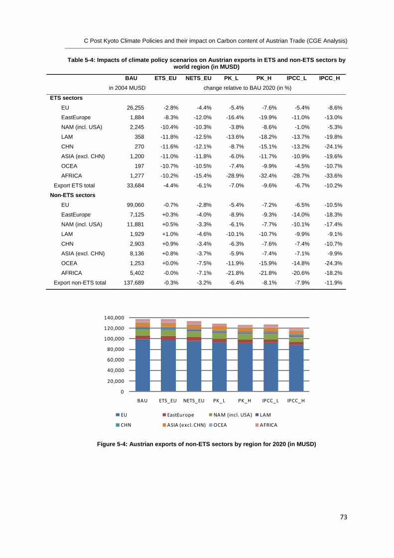
C Post Kyoto Climate Policies and their impact on Carbon content of Austrian Trade (CGE Analysis)
73
Table 5-4: Impacts of climate policy scenarios on Austrian exports in ETS and non-ETS sectors by world region (in MUSD)
BAU ETS_EU NETS_EU PK_L PK_H IPCC_L IPCC_H in 2004 MUSD change relative to BAU 2020 (in %)
ETS sectors
EU 26,255 -2.8% -4.4% -5.4% -7.6% -5.4% -8.6%
EastEurope 1,884 -8.3% -12.0% -16.4% -19.9% -11.0% -13.0%
NAM (incl. USA) 2,245 -10.4% -10.3% -3.8% -8.6% -1.0% -5.3%
LAM 358 -11.8% -12.5% -13.6% -18.2% -13.7% -19.8%
CHN 270 -11.6% -12.1% -8.7% -15.1% -13.2% -24.1%
ASIA (excl. CHN) 1,200 -11.0% -11.8% -6.0% -11.7% -10.9% -19.6%
OCEA 197 -10.7% -10.5% -7.4% -9.9% -4.5% -10.7%
AFRICA 1,277 -10.2% -15.4% -28.9% -32.4% -28.7% -33.6%
Export ETS total 33,684 -4.4% -6.1% -7.0% -9.6% -6.7% -10.2%
Non-ETS sectors
EU 99,060 -0.7% -2.8% -5.4% -7.2% -6.5% -10.5%
EastEurope 7,125 +0.3% -4.0% -8.9% -9.3% -14.0% -18.3%
NAM (incl. USA) 11,881 +0.5% -3.3% -6.1% -7.7% -10.1% -17.4%
LAM 1,929 +1.0% -4.6% -10.1% -10.7% -9.9% -9.1%
CHN 2,903 +0.9% -3.4% -6.3% -7.6% -7.4% -10.7%
ASIA (excl. CHN) 8,136 +0.8% -3.7% -5.9% -7.4% -7.1% -9.9%
OCEA 1,253 +0.0% -7.5% -11.9% -15.9% -14.8% -24.3%
AFRICA 5,402 -0.0% -7.1% -21.8% -21.8% -20.6% -18.2%
Export non-ETS total 137,689 -0.3% -3.2% -6.4% -8.1% -7.9% -11.9%
0
20,000
40,000
60,000
80,000
100,000
120,000
140,000
BAU ETS_EU NETS_EU PK_L PK_H IPCC_L IPCC_H
EU EastEurope NAM (incl. USA) LAM
CHN ASIA (excl. CHN) OCEA AFRICA
Figure 5-4: Austrian exports of non-ETS sectors by region for 2020 (in MUSD)

Carbon Content of Austrian International Trade
74
5.1 .3 Ef fec ts on Aus t r ian impor ts
With respect to imports, we find that Austrian imports of ETS sectors decline by 2.5% under
ETS_EU relative to BAU and decline by up to 14.9% under IPCC_H. Imports of non‐ETS sectors
decline by 0.5% under ETS_EU and by up to 7.1% under IPCC_H. Thus, overall imports are
slightly less declining under all climate policy scenarios than exports (but both more than
Austrian output). One explanation for the higher impact in ETS sectors relative to non‐ETS
sectors is the higher openness to trade in ETS sectors as well as the higher carbon intensity of
these sectors which lead to higher effects on relative prices compared to the non‐ETS sectors.
Furthermore, as Austria’s main trading partner – the rest of the EU – is subject to CO2 emission
caps as well, the import prices for ETS products from these countries tend to increase as well,
due to the pricing of carbon emissions. Among non‐ETS sectors, the imports of COA (coal) and
GAS decline sharpest which is also a consequence of the incentive provided by ETS to reduce
carbon emissions. All other non‐ETS sectors are affected much less. In ETS sectors, ELY
(electricity) and P_C (petroleum‐ and coke oven products) are affected much stronger than EIS
under all climate policy scenarios (Table 5‐5); again a feedback effect from reduced energy
demand in all sectors.
Table 5-5: Effects of climate policy scenarios on Austrian imports by sector relative to BAU 2020
BAU 2020 ETS_EU NETS_EU PK_L PK_H IPCC_L IPCC_H in 2004 MUSD change relative to BAU 2020 (in %)
ETS sectors
P_C 2,560 -1.7% -25.2% -37.1% -43.9% -40.2% -51.7%
ELY 1,400 -26.0% -26.5% -26.6% -34.9% -32.5% -45.2%
EIS 32,694 -1.6% -2.2% -4.0% -6.2% -5.6% -10.7%
ETS total 36,654 -2.5% -4.7% -7.2% -10.0% -9.0% -14.9%
Non-ETS sectors COA 238 -15.1% -28.2% -34.5% -42.4% -38.2% -49.7%
OIL 1,932 -2.6% -28.5% -34.9% -42.0% -38.2% -47.9%
GAS 932 -17.3% -20.4% -19.6% -27.7% -19.3% -29.8%
NEIS 88,673 -0.4% -1.3% -3.9% -5.4% -5.4% -9.1%
TRN 7,635 -0.2% +0.1% +5.5% +7.1% +2.4% +4.3%
FOOD 11,016 -0.1% -1.0% -2.0% -3.5% -3.0% -6.6%
SERV 45,824 -0.4% -0.7% -1.1% -2.3% -1.0% -2.7%
non-ETS total 156,249 -0.5% -1.5% -3.0% -4.4% -4.1% -7.1%
Import TMG 3,656 -0.8% -2.9% -5.8% -8.0% -7.6% -12.9%
Import total 196,558 -0.9% -2.1% -3.9% -5.5% -5.1% -8.6%

C Post Kyoto Climate Policies and their impact on Carbon content of Austrian Trade (CGE Analysis)
75
0
5,000
10,000
15,000
20,000
25,000
30,000
35,000
40,000
BAU ETS_EU NETS_EU PK_L PK_H IPCC_L IPCC_H
EU Eastern Europe NAM (incl. USA) LAM
CHN ASIA (excl. CHN) OCEANIA AFRICA
Figure 5-5: Austrian imports of ETS sectors by region for 2020 (in MUSD)
Austrian imports by region are summarized in Table 5‐6, Figure 5‐5 and Figure 5‐6. Again, the
main trading partner of Austria is the European Union, and hence the effects are strongest,
and roughly proportionally increasing with the strength of the policy, in absolute terms for
imports from other European countries. For other trading partners, there is however a
remarkable difference across scenarios: under the IPCC climate policy scenarios, both the US
and Russia are required to limit their emissions more strongly and hence imports from North
America (NAM, including US) and Eastern Europe drop under these scenarios much more than
under the other scenarios. A similar, but less pronounced effect is evident for CHN (China), the
rest of Asia, and Oceania.
0
20,000
40,000
60,000
80,000
100,000
120,000
140,000
160,000
BAU ETS_EU NETS_EU PK_L PK_H IPCC_L IPCC_H
EU EastEurope NAM (incl. USA) LAM
CHN ASIA (excl. CHN) OCEA AFRICA
Figure 5-6: Austrian imports of non-ETS sectors by region for 2020 (in MUSD)

Carbon Content of Austrian International Trade
76
Table 5-6: Effects of the scenarios on Austrian imports in ETS and non-ETS sectors by world region (in MUSD)
BAU 2020 ETS_EU NETS_EU PK_L PK_H IPCC_L IPCC_H
in 2004 MUSD change relative to BAU (in %)
ETS sectors
EU 33,376 -3.9% -6.2% -8.2% -11.4% -9.4% -15.1%
Eastern Europe 937 +12.0% +14.8% +17.0% +17.8% -3.2% -20.1%
NAM (incl. USA) 788 +10.8% +7.1% -9.6% -8.6% -21.3% -31.1%
LAM 169 +13.9% +10.8% +9.6% +13.6% +7.9% +12.3%
CHN 263 +11.9% +7.8% +1.7% +5.2% +1.6% +6.4%
ASIA (excl. CHN) 821 +11.3% +8.3% -7.1% -5.0% -4.6% -5.6%
OCEANIA 38 +14.0% +10.3% -6.1% -12.1% -22.3% -31.2%
AFRICA 260 +13.9% +14.3% +24.0% +26.8% +20.6% +21.1%
Import ETS total 36,654 -2.5% -4.7% -7.2% -10.0% -9.0% -14.9%
Non-ETS sectors
EU 115,124 -0.1% -1.4% -3.6% -4.9% -4.7% -7.8%
Eastern Europe 5,623 -3.3% -4.1% -5.4% -7.4% -6.5% -10.6%
NAM (incl. USA) 8,519 -1.4% -1.1% -4.2% -6.2% -3.4% -5.4%
LAM 1,934 -2.0% +1.6% +8.7% +9.1% +8.6% +8.7%
CHN 5,331 -1.2% -0.4% -1.2% -2.0% -1.5% -3.4%
ASIA (excl. CHN) 14,824 -1.3% -1.0% -3.0% -4.3% -3.7% -6.2%
OCEA 441 -1.2% +1.7% -4.1% -7.4% -7.4% -10.4%
AFRICA 4,453 -2.1% -5.5% +8.3% +6.5% +5.0% -0.0%
Imports Non-ETS total 156,249 -0.5% -1.5% -3.0% -4.4% -4.1% -7.1%
5.2 The carbon effects of the scenarios for Austria
The carbon emissions of the different scenarios are summarized in Table 5‐7 and Figure 5‐7
and Figure 5‐8. Emissions fall under all scenarios both according to the PBP and CBP, with
emissions (according to CBP) under IPCC_H almost halved compared to BAU. Moreover, while
carbon emissions under ETS_EU are reduced mainly by production, in all other scenarios
households also reduce their emissions, such that their share of total carbon emissions is
reduced from 24% in BAU to 19% in IPCC_H.

C Post Kyoto Climate Policies and their impact on Carbon content of Austrian Trade (CGE Analysis)
77
Table 5-7: CO2 effects according to the PBP and CBP of the scenarios relative to BAU 2020
Base 2020 ETS_EU NETS_EU PK_L PK_H IPCC_L IPCC_H Mt CO2 change relative to BAU 2020 (in %)
CO2 PrivHH 23.34 +3.8% -24.3% -39.6% -45.0% -42.7% -51.1%
CO2 Output 67.43 -12.1% -28.9% -37.1% -44.7% -40.5% -52.1%
PBP 90.77 -8.0% -27.7% -37.7% -44.8% -41.1% -51.8%
CO2 Import 31.25 -11.0% -12.3% -9.5% -12.4% -14.9% -22.0%
CO2 Export 22.09 -9.9% -29.1% -38.8% -46.6% -41.7% -53.2%
CO2 IM-EX 9.16 -13.8% +28.1% +61.3% +70.0% +49.9% +53.1%
CBP 99.93 -8.6% -22.6% -28.7% -34.3% -32.7% -42.2%
Moreover, the carbon trade balance improves for ETS_EU relative to BAU, but worsens in all
other scenarios. This implies that emissions from exports decline relative to emissions from
imports due to decreasing domestic output in combination with improved energy efficiency in
domestic production as well as a shift to imports from less regulated and therefore less
environmentally friendly producing regions as depicted in Table 5‐6.
0.00
20.00
40.00
60.00
80.00
100.00
120.00
2004 BAU ETS_EU NETS_EU PK_L PK_H IPCC_L IPCC_H
PBP CBP
Figure 5-7: PBP vs. CBP CO2 emissions for Austria 2020 (Mt CO2)
Additionally, a shift in the sectoral composition of imports to more non‐ETS and less ETS
commodities leaves the imported CO2 emissions at levels only 11% to 22% below BAU levels.
Figure 5‐9 illustrates that emissions embodied in imported non‐ETS commodities hardly
change in the policy scenarios compared to BAU, while the CO2 emissions linked to ETS imports

Carbon Content of Austrian International Trade
78
decrease substantially (by 35.5% in IPCC_H relative to BAU, see Table 5‐8). This is due to
generally reduced ETS imports and the, due to environmental regulations, lower CO2
intensities in ETS production of Austria’s main trading partners in the EU. Moving from the
unilateral EU scenarios ETS_EU and NETS_EU to more comprehensive climate policy scenarios,
Austria’s ETS import related CO2 emissions tend to go down even stronger, since also CO2
coefficients in the ETS production processes outside the EU are improved, caused by putting a
price tag on CO2 emissions.
0
20
40
60
80
100
120
2004 BAU ETS_EU NETS_EU PK_L PK_H IPCC_L IPCC_H
Output PrivHH IM‐EX
Figure 5-8: CO2 according to CBP for Austria 2020 (Mt CO2)
As mentioned earlier, the imported emissions embodied in NETS imports hardly change
compared to BAU even under the most stringent IPCC scenarios. This is caused by the fact that
a CO2 price does not put ancillary high pressure on the corresponding production costs, since
the non‐ETS sectors are reflected – by definition – by relatively low energy inputs in their
production processes. Furthermore the increasing CO2 emissions associated with imports of
transport services counterbalance the decreasing CO2 emissions from all other NETS sectors.
Austria tends to source out a substantial part of its transport sector – which is highly reactive
to changes in fossil fuel prices – to less regulated regions.

C Post Kyoto Climate Policies and their impact on Carbon content of Austrian Trade (CGE Analysis)
79
0
2
4
6
8
10
12
14
16
18
2004 BAU ETS_EU NETS_EU PK_L PK_H IPCC_L IPCC_H
IM ETS IM NETS EX ETS EX NETS
Figure 5-9: CO2 emissions in AUT trade 2020 (Mt CO2)
Table 5-8: Sectoral CO2 effects of the scenarios relative to BAU 2020 (Mt CO2)
Base 2020 ETS_EU NETS_EU PK_L PK_H IPCC_L IPCC_H
Mt CO2 Change relative to BAU 2020 (in %)
CO2 Output
P_C 0.58 -25.0% -44.9% -59.8% -68.2% -64.1% -75.3%
ELY 16.18 -22.8% -23.2% -20.1% -27.4% -23.2% -34.3%
EIS 15.67 -23.1% -22.4% -19.0% -27.7% -22.8% -36.4%
ETS total 32.42 -23.0% -23.2% -20.3% -28.3% -23.7% -36.0%
COA 0.00 - - - - - -
OIL 0.06 -1.6% -61.3% -95.7% -97.7% -97.1% -99.1%
GAS 0.15 -0.3% -84.6% -97.4% -98.6% -99.7% -100.0%
NEIS 2.43 -5.0% -38.8% -55.4% -62.1% -59.5% -69.6%
TRN 21.70 -0.6% -32.4% -51.7% -59.3% -54.7% -65.9%
FOOD 3.04 -2.9% -40.9% -58.7% -65.0% -62.3% -71.7%
SERV 7.63 -5.0% -33.6% -50.8% -58.2% -55.1% -66.2%
CGDS 0.00 - - - - - -
non-ETS total 35.01 -2.0% -34.1% -52.6% -60.0% -56.1% -66.9%
Output total 67.43 -12.1% -28.9% -37.1% -44.7% -40.5% -52.1%

Carbon Content of Austrian International Trade
80
Table 5-8 (cont.): Sectoral CO2 effects of the scenarios relative to BAU 2020 (Mt CO2)
Base 2020 ETS_EU NETS_EU PK_L PK_H IPCC_L IPCC_H
Mt CO2 Change relative to BAU (in %)
CO2 Exports
P_C 0.04 -26.3% -39.4% -51.3% -61.3% -56.6% -70.4% ELY 1.89 -15.5% -14.7% -10.7% -15.9% -10.6% -18.9% EIS 7.10 -24.1% -24.0% -21.2% -30.3% -24.7% -38.3%
ETS total 9.03 -22.3% -22.1% -19.2% -27.4% -21.9% -34.4% COA 0.00 - - - - - - OIL 0.00 +2.3% -46.4% -68.0% -71.7% -67.6% -72.4% GAS 0.02 -5.8% -66.3% -85.7% -89.3% -82.4% -82.8% NEIS 1.27 -4.9% -39.4% -56.6% -63.3% -61.0% -71.2% TRN 5.88 -0.5% -36.1% -56.5% -64.7% -58.1% -69.6% FOOD 0.63 -2.7% -42.0% -60.2% -66.5% -64.0% -73.3% SERV 0.81 -4.9% -33.4% -50.6% -57.7% -55.1% -66.0%
non-ETS total 8.60 -1.7% -36.8% -56.3% -64.0% -58.7% -69.8% CO2 TRANS 4.46 -0.5% -28.4% -45.0% -51.8% -49.0% -59.2%
Exports total 22.09 -9.9% -29.1% -38.8% -46.6% -41.7% -53.2% CO2 Imports
P_C 0.21 -20.8% -41.4% -56.9% -65% -62% +600% ELY 5.60 -38.8% -39.4% -38.8% -46.2% -44.8% -37.6% EIS 9.94 -8.6% -6.7% -3.8% -9.2% -11.5% -47.9%
ETS total 15.75 -19.5% -18.8% -17.0% -23.1% -24.0% -35.5% COA 0.05 -26.0% -52.2% -62.3% -71.1% -67.4% -78.6% OIL 0.23 -0.0% -22.7% -34.6% -41.7% -38.6% -53.8% GAS 0.81 -20.7% -29.3% -27.8% -32.2% -34.5% -53.5% NEIS 2.02 -4.2% -17.8% -27.5% -33.7% -33.7% -33.1% TRN 7.44 -0.3% +6.0% +21.1% +28.2% +19.5% +25.2% FOOD 0.79 -3.3% -26.4% -34.5% -42.3% -40.9% -57.7% SERV 1.23 -3.3% -13.3% -19.7% -25.4% -24.6% -43.9%
non-ETS total 12.56 -2.8% -4.8% +1.3% +3.0% -2.0% -3.1% CO2 IM TMG 2.93 -0.6% -9.9% -15.6% -20.7% -20.6% -31.1%
Imports total 31.25 -11.0% -12.3% -9.5% -12.4% -14.9% -22.0%

C Post Kyoto Climate Policies and their impact on Carbon content of Austrian Trade (CGE Analysis)
81
5.3 The economic and carbon effects of the scenarios on a global scale
In the previous sections we have dealt with the repercussions of climate policies on the
Austrian economy in the EU context as well as in a broader post‐Kyoto context respectively. In
the subsequent sections we are going to refocus our analysis by taking a look at the global
effects of the different scenarios. Obviously, one distinctive feature of the different scenarios
is the regional scope – reaching from ‘unilateral’ EU policies to broader ones which cover the
Annex I countries. Since our analysis is based on plausible developments, none of the scenarios
is of global scope with binding agreements also for developing countries. Another distinctive
feature of the scenarios is the sectoral scope of the emission reduction obligations, with
EU_ETS being limited to ETS sector emissions while all other scenarios require limitations for
non‐ETS sectors too. Obviously, both the limited regional and the limited sectoral scope might
lead to inefficiencies, discussed under the heading of competitiveness and carbon leakage. We
will thus investigate the economic as well as the environmental ramifications on a global scale
and illustrate our findings on the relevance of carbon leakage in this context.
Table 5-9: Annual GDP growth rates for 2020 for the scenarios
1999-2008 BAU 2020 ETS_EU NETS_EU PK_L PK_H IPCC_L IPCC_H
AUT 2.40 2.19 2.16 2.09 1.95 1.84 1.90 1.66 GER 1.49 2.39 2.36 2.27 2.31 2.24 2.28 2.12 ITA 1.22 1.81 1.78 1.73 1.64 1.54 1.60 1.37 WEU 2.41 2.36 2.34 2.27 2.12 2.01 2.07 1.84 SEEU 4.18 2.83 2.75 2.73 2.68 2.56 2.61 2.34 NEU 2.74 2.59 2.57 2.48 2.46 2.37 2.42 2.23 RUS 6.85 2.52 2.50 2.44 2.35 2.33 2.34 2.22 ROE 3.94 2.57 2.57 2.58 2.45 2.43 1.67 1.37 GUS 7.72 3.09 3.08 3.06 2.97 2.93 2.90 2.63 USA 2.62 2.57 2.57 2.57 2.46 2.44 2.28 2.02 NAM 2.95 2.91 2.91 2.92 2.70 2.69 2.58 2.44 LAM 3.50 1.32 1.32 1.32 1.31 1.31 1.31 1.28 CHN 9.76 5.90 5.91 5.90 5.90 5.89 5.89 5.85 EASI 1.89 2.43 2.43 2.43 2.23 2.22 2.30 2.23 SEAS 5.02 5.38 5.39 5.39 5.39 5.37 5.37 5.32 SASI 6.72 4.14 4.15 4.15 4.17 4.17 4.17 4.15 OCEA 3.18 2.99 2.99 2.99 2.84 2.69 2.53 2.22 MENA 5.10 1.78 1.79 1.77 1.69 1.68 1.69 1.65 SSA 4.16 1.16 1.16 1.15 1.12 1.11 1.11 1.07

Carbon Content of Austrian International Trade
82
5.3 .1 The e f fec ts on GDP
The first part of our analysis of the global effects of different climate policy scenarios focuses
on the economic impacts. As a measure for the economic performance of a region we utilize
the GDP growth rate, which is presented for all regions and all scenarios in Table 5‐9. The first
column represents the regions’ average annual GDP growth rates over the period 1999 to
2008, derived from IMF (2009) data. The second column shows our model results for the GDP
growth rate under BAU assumptions, therefore without any climate policy measures.
Compared to the 1999‐2008 average growth rates, these 2020 GDP growth rates are in most
cases lower, representing the highly visible impacts of the current economic downturn. China’s
predicted economic growth is 3.86 percentage points lower (5.90%) than in the comparison
period (9.76%). Also Latin American and African economies, which are already facing hard
times in the globalized world economy due to lack of capital and productivity drawbacks
(reflected by low MFP, capital and labor force growth rates in Table 2‐3), will be substantially
affected by the crises ramifications. Within the EU, South Eastern European countries will be
mostly affected by the economic downswing, the average annual GDP growth rates falling in
BAU by 1.35 percentage points to a level of 2.83%.
The impacts of climate policies may alter these effects, as our model results illustrate. In the
ETS_EU and NETS_EU scenarios, only the EU is faced by binding emission constraints. In the
ETS_EU scenario, almost no consequences on GDP growth rates arise for all other countries
(reducing only EU’s annual average GDP growth rate slightly compared to BAU due to EU wide
emissions trading). In the NETS_EU scenario, where the EU restricts GHG emissions to a level
of 20% below 2005 levels, stronger consequences for worldwide economic growth arise. These
reduced growth rates are mostly triggered by high carbon prices in the NETS sectors.
Moreover, while the ETS sector is responsible of approximately 13% of output and 80% of
carbon emissions in the EU, the inclusion of the NETS sectors and households implies a much
stronger reduction of final demand. Additionally, emissions reductions within these sectors
and by households cannot be traded within the EU as in the ETS sectors, additionally increasing
the carbon price compared to the ETS sector. Despite the strong economic consequences
within the EU, the non‐abating regions outside the EU are not affected by these slowdowns of
economic growth within the EU, or may even benefit, as was shown in section 5.1.3 by means
of increasing imports especially from non‐EU ETS sectors.
Only when all Annex I regions’ CO2 emissions are affected by a more comprehensive global
climate agreement (PK and IPCC scenarios), countries like the USA, Japan or Ukraine have to
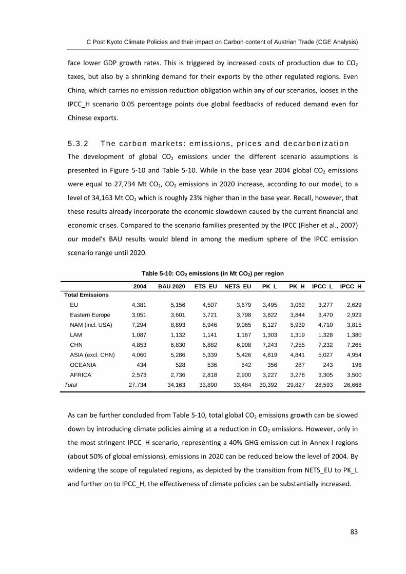
C Post Kyoto Climate Policies and their impact on Carbon content of Austrian Trade (CGE Analysis)
83
face lower GDP growth rates. This is triggered by increased costs of production due to CO2
taxes, but also by a shrinking demand for their exports by the other regulated regions. Even
China, which carries no emission reduction obligation within any of our scenarios, looses in the
IPCC_H scenario 0.05 percentage points due global feedbacks of reduced demand even for
Chinese exports.
5.3 .2 The carbon markets : emiss ions , pr ices and decarbon iza t ion
The development of global CO2 emissions under the different scenario assumptions is
presented in Figure 5‐10 and Table 5‐10. While in the base year 2004 global CO2 emissions
were equal to 27,734 Mt CO2, CO2 emissions in 2020 increase, according to our model, to a
level of 34,163 Mt CO2 which is roughly 23% higher than in the base year. Recall, however, that
these results already incorporate the economic slowdown caused by the current financial and
economic crises. Compared to the scenario families presented by the IPCC (Fisher et al., 2007)
our model’s BAU results would blend in among the medium sphere of the IPCC emission
scenario range until 2020.
Table 5-10: CO2 emissions (in Mt CO2) per region
2004 BAU 2020 ETS_EU NETS_EU PK_L PK_H IPCC_L IPCC_H Total Emissions
EU 4,381 5,156 4,507 3,679 3,495 3,062 3,277 2,629
Eastern Europe 3,051 3,601 3,721 3,798 3,822 3,844 3,470 2,929
NAM (incl. USA) 7,294 8,893 8,946 9,065 6,127 5,939 4,710 3,815
LAM 1,087 1,132 1,141 1,167 1,303 1,319 1,328 1,380
CHN 4,853 6,830 6,882 6,908 7,243 7,255 7,232 7,265
ASIA (excl. CHN) 4,060 5,286 5,339 5,426 4,819 4,841 5,027 4,954
OCEANIA 434 528 536 542 356 287 243 196
AFRICA 2,573 2,736 2,818 2,900 3,227 3,278 3,305 3,500
Total 27,734 34,163 33,890 33,484 30,392 29,827 28,593 26,668
As can be further concluded from Table 5‐10, total global CO2 emissions growth can be slowed
down by introducing climate policies aiming at a reduction in CO2 emissions. However, only in
the most stringent IPCC_H scenario, representing a 40% GHG emission cut in Annex I regions
(about 50% of global emissions), emissions in 2020 can be reduced below the level of 2004. By
widening the scope of regulated regions, as depicted by the transition from NETS_EU to PK_L
and further on to IPCC_H, the effectiveness of climate policies can be substantially increased.

Carbon Content of Austrian International Trade
84
However, as more regions beyond the EU have to reduce their CO2 emissions, the countries
still not included within an emission mitigation agreement increase their emissions compared
to 2004 by far more than the abating regions reduce their emissions. For instance, China’s CO2
emissions in the IPCC_H scenario increase by 2,400 Mt CO2 by 2020, while the EU’s CO2
emissions can only be reduced by 1,750 Mt CO2.
‐8,000
‐6,000
‐4,000
‐2,000
+0
+2,000
+4,000
+6,000
+8,000
ETS_EU NETS_EU PK_L PK_H IPCC_L IPCC_H
EU Eastern Europe NAM (incl. USA) LAM CHN ASIA (excl. CHN) OCEANIA AFRICA
Figure 5-10: Change in CO2 emissions (in Mt CO2) per region and per scenario relative to 2004
Figure 5‐10 illustrates the global carbon effects of the different policy scenarios, with a focus
on how emissions change in the different regions. As argued above, the decrease of CO2
emissions in abating regions compared to 2004 is more than counterbalanced in any scenario –
except of IPCC_H – in this paper. In the least stringent scenario (ETS_EU), 2020 emissions
increase in all regions compared to base year 2004, including the abating region (EU). This
follows from a relative stronger increase in CO2 emissions in the not regulated NETS sectors
and the private households, which outweigh emission reductions in the ETS sectors. These
higher NETS emissions in the EU can be overcome by incorporating the NETS sectors and the
private households into the EU’s abatement efforts. When all Annex I regions are subject to
emission constraints (starting with PK_L) climate policies become more successful in reducing
emissions on a global scale. A major contribution originates from the regulation of North
America’s (incl. USA) CO2 emissions, though these efforts are still outperformed by China’s CO2
emissions increase.

C Post Kyoto Climate Policies and their impact on Carbon content of Austrian Trade (CGE Analysis)
85
The CO2 permit prices associated with the various CO2 emission reduction scenarios are
presented in Table 5‐11. It can be seen that in all scenarios the ETS permit prices are equal
across the EU, representing the implementation of an emissions trading scheme (ETS) in the
European Union.
Table 5-11: CO2 price in ETS sectors per region (in USD/tCO2)
ETS_EU NETS_EU PK_L PK_H IPCC_L IPCC_H ETS sectors AUT 130 124 100 166 135 282 GER 130 124 100 166 135 282 ITA 130 124 100 166 135 282 WEU 130 124 100 166 135 282 SEEU 130 124 100 166 135 282 NEU 130 124 100 166 135 282 RUS - - - - 13 35 ROE - - 36 38 245 310 GUS - - - - 4 12 USA - - 84 95 229 410 NAM - - 120 119 184 251 LAM - - - - - - CHN - - - - - - EASI - - 195 188 112 162 SEAS - - - - - - SASI - - - - - - OCEA - - 63 130 209 338 MENA - - - - - - SSA - - - - - -
When NETS sectors’ as well as private households’ CO2 emissions are regulated too (NETS_EU),
the EU wide CO2 permit price for ETS sectors decreases to 124 USD/tCO2, due to reduced
production triggered by the falling demand by the henceforth constrained NETS sectors and
private households. The CO2 shadow prices for these agents, depicted in Table 5‐12 , are
notably higher than the ETS permit prices. This is not only due to the absence of an EU‐wide
market for the NETS emission allowances, as can be concluded from comparing non‐EU prices
for ETS and NETS permits (which are in every region higher); this result confirms the more
difficult reduction of CO2 emissions found in reality for private households and non‐energy
intensive sectors – most prominently emissions related to transport. When moving from
scenarios in which emission constraints are introduced only in an EU context, to semi‐universal
post‐Kyoto scenarios, the EU ETS‐permit prices experience another drop from the above
mentioned 124 USD/tCO2 to 100 USD/tCO2. This effect is triggered on the one hand by more
efficient production processes as a response to stricter emission constraints and on the other

Carbon Content of Austrian International Trade
86
hand by a shrinking foreign demand from countries which were previously not affected by
climate policies. As more ambitious reduction targets are introduced in the scenarios, emission
permits become more expensive – both in the ETS and the NETS sectors.
Table 5-12: CO2 price in non-ETS sectors per region (in USD/tCO2)
NETS_EU PK_L PK_H IPCC_L IPCC_H AUT 395 1065 1507 1300 2246 GER 449 332 521 442 874 ITA 341 847 1276 1030 1972 WEU 368 1117 1569 1342 2282 SEEU 71 228 381 310 638 NEU 426 550 827 692 1280 RUS - - - 12 58 ROE - 226 239 1381 1760 GUS - 25 23 40 56 USA - 329 366 808 1439 NAM - 250 245 345 437 LAM - - - - - CHN - - - - - EASI - 756 744 502 688 SEAS - - - - - SASI - - - - - OCEA - 480 872 1351 2136 MENA - - - - - SSA - - - - -
Eastern European regions (ROE and GUS) and Russia can be identified as the cheapest
destination for emission reduction, since these countries are characterized by highly carbon
intensive production processes in the base year 2004, leaving enough space for efficiency
improvements for 2020. This conjecture can be confirmed by an analysis of CO2 intensities in
the different regions and sectors and leads to the question whether the introduction of climate
policies accelerates the decarbonization of societies.

C Post Kyoto Climate Policies and their impact on Carbon content of Austrian Trade (CGE Analysis)
87
Table 5‐13 presents the carbon intensities, or the CO2 coefficients, per country and sector for
the year 2020 under BAU, which were calculated as the total carbon input in the various
production processes divided by total output of the respective sector.
Table 5-13: CO2 coefficients (in t CO2 per MUSD) per country and sector for BAU 2020
P_C ELY EIS COA OIL GAS NEIS TRN FOOD CO2 coefficient in t CO2 per 2004 MUSD
AUT 132 2,124 219 0 205 444 16 431 73
GER 15 3,410 204 16 202 65 10 519 45
ITA 5 2,758 188 23 203 14 21 635 72
WEU 166 2,288 174 19 74 66 15 694 76
SEEU 166 6,718 456 205 847 1,395 27 725 108
NEU 502 2,949 162 55 153 430 18 440 57
RUS 345 13,832 2,036 198 147 590 90 2,508 185
ROE 38 4,765 915 16 132 756 74 661 160
GUS 416 6,561 7,603 91 269 297 481 1,580 324
USA 561 7,087 336 26 265 292 26 1,519 124
NAM 922 4,630 395 444 340 896 48 1,932 79
LAM 399 2,696 754 118 267 1,690 62 1,817 108
CHN 28 17,805 1,302 1,343 667 16,328 77 1,039 290
EASI 64 3,089 231 38 85 1,875 16 479 92
SEAS 376 5,107 591 110 64 106 35 1,124 103
SASI 151 9,139 1,990 243 212 374 65 937 85
OCEA 188 8,055 416 174 307 552 48 842 83
MENA 2,075 9,189 2,396 170 69 452 209 2,261 156
SSA 237 14,618 964 14 85 4,271 93 1,502 54
These CO2 coefficients differ quite substantially across regions, with the highest differences in
the electricity, and energy intensive sectors. By a comparison among regions – visualized in
Figure 5‐11 – it is striking that CO2 intensities in these sectors are by far highest in China,
followed by Southeast Europe, Russia and the developing countries in Asia and Africa,
reflecting the disproportionally high CO2 intensities in these countries production methods.
While Austria’s EIS sector for example emits 219 tCO2 per MUSD output, the GUS region emits
34 times as much CO2 for the same amount of output.

Carbon Content of Austrian International Trade
88
0
2,000
4,000
6,000
8,000
10,000
12,000
14,000
16,000
18,000
20,000
AUT GER ITA WEU SEEU NEU RUS ROE GUS USA NAM LAM CHN EASI SEAS SASI OCEA MENA SSA
P_C ELY EIS COA OIL GAS NEIS TRN FOOD
Figure 5-11: CO2 coefficients for BAU 2020 across countries and sectors (t CO2/MUSD)
Comparing Table 5‐13 to Table 5‐14 shows that more stringent mitigation efforts in the sense
of stricter carbon emission constraints also trigger a more efficient usage of fossil fuels in
production. By taxing the release of CO2 due to combustion of fossil fuels or in industrial
processes, industries as well as private households have an incentive to reduce their carbon
emissions either by directly reducing the fossil fuel consumption or by raising energy
efficiency. This decarbonization effect can reduce sectoral country specific CO2 coefficients by
a quite substantial amount. Austria’s emission intensity in the power generation sector (ELY)
for example would be reduced by 605 tCO2/MUSD, thus representing a shift to more
renewable energy as well as an increase in energy efficiency in fossil fueled power plants.
The important issue of power generation is analyzed in more detail in Figure 5‐12. There we
see that both the PK and IPCC scenarios lead to improvements in energy efficiency in power
generation in all Annex I countries, namely USA, the remaining North America, Oceania (i.e.
Australia, New Zealand), East Asia (i.e. Japan), and all EU countries. In contrast, all other
countries, namely Russia China and the remaining American, Asian and African regions do not
experience any considerably improvements compared to BAU 2020. In Sub‐Saharan African
countries the CO2 intensity of the power generation sector even tends to increase, compared
to BAU, since this region does not face any carbon price induced incentives to increase energy
efficiency. The effect of the NETS_EU scenario on improved energy efficiency is only apparent
for the EU countries, showing the limited scope of solving a global problem unilaterally.
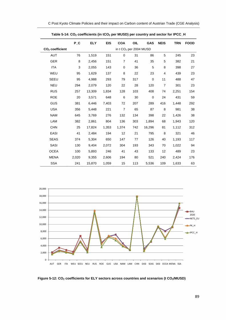
C Post Kyoto Climate Policies and their impact on Carbon content of Austrian Trade (CGE Analysis)
89
Table 5-14: CO2 coefficients (in tCO2 per MUSD) per country and sector for IPCC_H
P_C ELY EIS COA OIL GAS NEIS TRN FOOD
CO2 coefficient in t CO2 per 2004 MUSD
AUT 76 1,519 151 0 31 86 5 245 23
GER 8 2,456 151 7 41 35 5 382 21
ITA 3 2,055 143 0 36 5 8 398 27
WEU 95 1,629 137 8 22 23 4 439 23
SEEU 95 4,988 293 79 317 0 11 488 47
NEU 294 2,079 120 22 28 120 7 301 23
RUS 257 13,309 1,834 128 103 408 74 2,251 154
ROE 20 3,571 648 6 30 0 24 431 59
GUS 381 6,446 7,403 72 207 289 416 1,448 292
USA 356 5,448 221 7 65 87 8 981 38
NAM 645 3,769 276 132 134 398 22 1,426 38
LAM 382 2,861 804 136 303 1,894 68 1,943 120
CHN 25 17,824 1,353 1,374 742 16,296 81 1,112 312
EASI 41 2,484 194 12 21 795 8 321 46
SEAS 374 5,304 650 147 77 126 40 1,193 117
SASI 130 9,404 2,072 304 193 343 70 1,022 94
OCEA 100 5,893 246 41 43 133 12 489 23
MENA 2,020 9,355 2,606 194 80 521 240 2,424 176
SSA 241 15,870 1,059 15 113 5,536 109 1,633 63
0
2,000
4,000
6,000
8,000
10,000
12,000
14,000
16,000
18,000
20,000
AUT GER ITA WEU SEEU NEU RUS ROE GUS USA NAM LAM CHN EASI SEAS SASI OCEA MENA SSA
BAU 2020
NETS_EU
PK_H
IPCC_H
Figure 5-12: CO2 coefficients for ELY sectors across countries and scenarios (t CO2/MUSD)

Carbon Content of Austrian International Trade
90
5.3 .3 Carbon Leakage
A fiercely discussed issue in the climate policy debate is the carbon leakage phenomenon – a
partial offset of domestically reduced GHG emissions in countries with less stringent
environmental requirements as a result of a relocation of production to regions not facing
mitigation policies.
Table 5‐15 presents the implications of climate policies on GHG abating countries – the policy‐
regions – as well as on non‐abating or non‐policy regions. Two different policy region
groupings for the base year 2004 are necessary, since the two unilateral EU scenarios embrace
fewer regions than the post‐Kyoto and the IPCC scenarios. The changes in CO2 emissions in the
respective scenarios were calculated as the difference between the policy regions’ and the
non‐policy regions’ 2020 emissions and their respective CO2 emissions in the base year 2004.
Thus e.g. in the NETS_EU scenario the change in CO2 emissions of ‐703 Mt CO2 results from an
emission reduction in abating regions from 4,381 Mt CO2 in 2004 to 3,679 Mt CO2 in 2020.
However, the net change in total global CO2 emissions for the NETS_EU setting is still
significantly positive – due to increasing emissions in the non abating regions by 6,452 Mt CO2.
Table 5-15: CO2 effects (in Mt CO2) of climate policies relative to 2004
2004 ETS_EU NETS_EU 2004 PK_L PK_H IPCC_L IPCC_H CO2 emissions
policy regions 4,381 4,507 3,679 17,263 15,316 14,649 13,412 11,124
Non-policy regions 23,353 29,382 29,805 10,471 15,076 15,178 15,180 15,544
Total 27,734 33,890 33,484 27,734 30,392 29,827 28,593 26,668
Change relative to 2004
policy regions +126 -703 -1,948 -2,615 -3,851 -6,139
non policy regions +6,029 +6,452 +4,605 +4,707 +4,710 +5,073
Total +6,155 +5,750 +2,658 +2,093 +858 -1,066
The first salient conclusion that can be drawn from Table 5‐15 is that in the ETS_EU as well as
the NETS_EU settings only about one sixth of the world’s 2020 CO2 emissions under BAU
assumptions would be regulated by climate policies. Therefore even under the successful
implementation of the EU 20‐20 targets in the NETS_EU scenario, thereby reducing the EU’s
CO2 emissions by 20% compared to 2005 emissions (European Commission, 2008), the global
effect would be a substantial increase of CO2 emissions compared to 2004 by 5.8 Gt CO2. The

C Post Kyoto Climate Policies and their impact on Carbon content of Austrian Trade (CGE Analysis)
91
total global emissions in 2020 under the NETS_EU scenario would still be boosted to 33.5 Gt
CO2, only 0.4 Gt CO2 below BAU.
Under a more comprehensive climate policy agreement comprising all Annex I countries of the
UNFCCC Kyoto Protocol – represented by the two post‐Kyoto and IPCC scenarios – more
fundamental reduction achievements could be obtained, since more than 50% of global 2004
CO2 emissions would be regulated in such a policy framework. However, only in the most
stringent policy scenario – IPCC_H with a reduction of Annex I regions’ emissions by 40% until
2020 compared to 1990 levels – the global net effect would be a decline in emissions
compared to 2004 levels, since non‐abating regions’ emissions would grow by 1 Gt CO2 less
than the reduction in Annex I countries (see bottom row of Table 5‐15). Under these
circumstances carbon leakage is very likely to occur.
Following a ‘strong’ definition of carbon leakage, the increase of CO2 emissions beyond BAU in
non‐abating regions is divided by the emission reduction relative to BAU in the abating regions
to get a measure for the amount of carbon emissions which is leaking by production shifts to
other regions and hence counteract the emission reductions in the abating countries. These
shares are depicted for our scenarios in the bottom line of Table 5‐16 (which contains the
same information as Table 5‐15, with the difference that the scenarios’ results are compared
to BAU 2020 and not the base year 2004).
Table 5-16: Climate policies and carbon leakage - Global CO2 effects relative to 2020 (in Mt CO2)
BAU ETS_EU NETS_EU BAU PK_L PK_H IPCC_L IPCC_H CO2 emissions
policy regions 5,156 4,507 3,679 20,556 15,316 14,649 13,412 11,124
non-policy regions 29,007 29,382 29,805 13,607 15,076 15,178 15,180 15,544
Total 34,163 33,890 33,484 34,163 30,392 29,827 28,593 26,668
Change relative to 2020
policy regions -649 -1,478 -5,241 -5,907 -7,144 -9,432
non policy regions +375 +799 +1,469 +1,571 +1,574 +1,937
2020 Total -274 -679 -3,771 -4,336 -5,571 -7,495
Leakage rate 2020 -58% -54% -28% -27% -22% -21%
Figure 5‐13 compares the abating regions’ CO2 reduction achievements (relative to BAU 2020)
to the increase of CO2 emissions in the regions not facing GHG emission constraints, again
relative to BAU. By comparing the CO2 effects in this figure (as well as in Table 5‐16) to the
2020 emissions under BAU presumptions, the ancillary CO2 effect on non‐abating regions

Carbon Content of Austrian International Trade
92
triggered by not globally set emission constraints can be deducted. It turns out that part of the
policy induced CO2 emissions reductions are offset by emission increases in non‐policy regions,
ranging from ‐21% for IPCC_H to ‐58% for ETS_EU. Thus, under ETS_EU more than half of the
emission reduction within the EU is counteracted by ancillary emission increases above BAU in
non‐abating countries.
‐12,000
‐10,000
‐8,000
‐6,000
‐4,000
‐2,000
+0
+2,000
+4,000
ETS_EU NETS_EU PK_L PK_H IPCC_L IPCC_H
policy regions non policy regions
Figure 5-13: CO2 effects (in Mt CO2) in abating and non-abating regions relative to BAU-2020
The derived carbon leakage rates amount to ‐58% in the ETS_EU scenario and ‐54% in the
NETS_EU scenario respectively. This is due to the fact, which has already been pointed out
earlier, that only a small fraction of global CO2 emissions is under control in these unilateral EU
scenarios. The fraction of abated CO2 emissions, offset in non‐abating regions, declines, the
more stringent and comprehensive the climate policies become. But even in the most
stringent and comprehensive climate policy scenario IPCC_H, carbon leakage amounts to ‐21%.

C Post Kyoto Climate Policies and their impact on Carbon content of Austrian Trade (CGE Analysis)
93
Table 5-17: Change in emissions (in %) relative to BAU
2004 BAU 2020 ETS_EU NETS_EU PK_L PK_H IPCC_L IPCC_H
EU 4,381 5,156 -12.6% -28.7% -32.2% -40.6% -36.5% -49.0%
Eastern Europe 3,051 3,601 +3.3% +5.5% +6.1% +6.8% -3.6% -18.7%
NAM (incl. USA) 7,294 8,893 +0.6% +1.9% -31.1% -33.2% -47.0% -57.1%
LAM 1,087 1,132 +0.8% +3.1% +15.1% +16.6% +17.3% +21.9%
CHN 4,853 6,830 +0.8% +1.1% +6.0% +6.2% +5.9% +6.4%
ASIA (excl. CHN) 4,060 5,286 +1.0% +2.6% -8.8% -8.4% -4.9% -6.3%
OCEA 434 528 +1.5% +2.6% -32.6% -45.7% -53.9% -63.0%
AFRICA 2,573 2,736 +3.0% +6.0% +18.0% +19.8% +20.8% +28.0%
Total 27,734 34,163 -0.8% -2.0% -11.0% -12.7% -16.3% -21.9%
The more parties are being held responsible for their CO2 emissions, the less room is left for
emissions leaking to non‐regulated regions. As can be seen in Figure 5‐14, CO2 emissions in the
post‐Kyoto and the IPCC scenarios are only increasing relative to BAU in Latin America, China
and Africa – regions which are not facing any emission constraints in any of the scenarios and
whose emissions can therefore grow without bounds. The more stringent the reduction
objectives become, the higher the CO2 reduction achievements in regions like North America
or Eastern Europe become.
‐10,000
‐8,000
‐6,000
‐4,000
‐2,000
+0
+2,000
ETS_EU NETS_EU PK_L PK_H IPCC_L IPCC_H
EU Eastern Europe NAM (incl. USA) LAM CHN ASIA (excl. CHN) OCEANIA AFRICA
Figure 5-14: Change in CO2 emissions (in Mt CO2) relative to BAU
Table 5‐17 gives a more detailed account of CO2 emission trajectories in the presence of
climate policies. While emissions compared to BAU in most regions fall quite significantly,
moving from the least to the most stringent scenario, the picture in China, Latin America and
Africa is quite different. The EU’s CO2 emissions reduction would increase from ‐13% in the

Carbon Content of Austrian International Trade
94
ETS_EU scenario to ‐49% compared to 2020 BAU assumptions. Even in North America
(including USA), where emissions would rise in the two EU scenarios due to carbon leakage
even more than under BAU, CO2 emissions would fall by 57% in the strict IPCC_H setting
compared to BAU. For China on the other hand, CO2 emissions would be subject to even a
more accelerated growth than under BAU premise, fostering emission growth by 6.4% in the
IPCC_H scenario relative to BAU. For Africa and Latin America these carbon leakage induced
CO2 effects are even stronger, though these regions are starting from substantially lower CO2
emissions in the base year 2004 – 1,087 Mt CO2 for LAM and 2,573 Mt CO2 for AFRICA
compared to 4,853 for CHN (Table 5‐17).
Table 5-18: Sectoral CO2 effects and carbon leakage (in Mt CO2) relative to BAU
BAU ETS_EU NETS_EU BAU PK_L PK_H IPCC_L IPCC_H in Mt CO2 relative to BAU 2020 relative to BAU 2020
policy regions ETS sectors
P_C 71 -18 -27 409 -167 -181 -221 -268 ELY 1552 -525 -526 7243 -1,674 -1,911 -2,395 -3,193 EIS 735 -155 -144 2765 -220 -311 -474 -885
Non-ETS sectors COA 2 -1 -1 9 -4 -5 -5 -6 OIL 14 +1 -9 88 -46 -49 -56 -66 GAS 18 +0 -12 132 -65 -68 -79 -98 NEIS 97 -7 -36 336 -135 -148 -164 -199 TRN 1023 -8 -290 3712 -1,161 -1,283 -1,519 -1,935 FOOD 197 -8 -70 584 -244 -268 -297 -358 SERV 279 -19 -98 1204 -448 -489 -552 -687
Private households 1167 +89 -264 4075 -1,079 -1,195 -1,380 -1,737 non-policy regions ETS sectors
P_C 717 +9 +22 379 +49 +56 +63 +98 ELY 11,072 +204 +235 5381 +331 +346 +330 +384 EIS 5,254 +121 +203 3224 +402 +411 +396 +433
Non-ETS sectors COA 101 +1 +1 94 +4 +4 +3 +3 OIL 163 +1 +4 89 +11 +11 +11 +13 GAS 256 +3 +6 142 +9 +9 +9 +11 NEIS 637 +4 +12 399 +38 +34 +30 +16 TRN 4,135 +10 +236 1447 +474 +553 +578 +835 FOOD 866 +4 +19 479 +47 +46 +46 +42 SERV 1,346 +7 +21 421 +32 +31 +32 +30
Private households 4,459 +12 +42 1551 +72 +71 +74 +72 Total 34,163 -274 -679 34,163 -3,771 -4,336 -5,571 -7,495
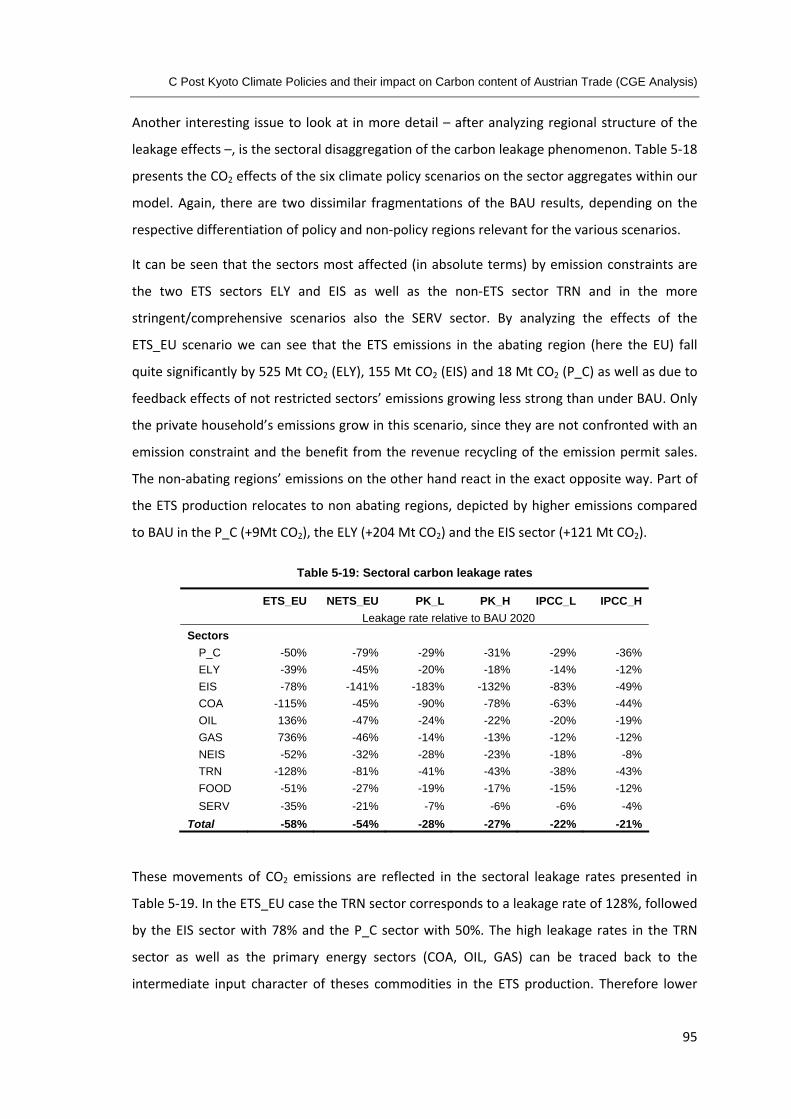
C Post Kyoto Climate Policies and their impact on Carbon content of Austrian Trade (CGE Analysis)
95
Another interesting issue to look at in more detail – after analyzing regional structure of the
leakage effects –, is the sectoral disaggregation of the carbon leakage phenomenon. Table 5‐18
presents the CO2 effects of the six climate policy scenarios on the sector aggregates within our
model. Again, there are two dissimilar fragmentations of the BAU results, depending on the
respective differentiation of policy and non‐policy regions relevant for the various scenarios.
It can be seen that the sectors most affected (in absolute terms) by emission constraints are
the two ETS sectors ELY and EIS as well as the non‐ETS sector TRN and in the more
stringent/comprehensive scenarios also the SERV sector. By analyzing the effects of the
ETS_EU scenario we can see that the ETS emissions in the abating region (here the EU) fall
quite significantly by 525 Mt CO2 (ELY), 155 Mt CO2 (EIS) and 18 Mt CO2 (P_C) as well as due to
feedback effects of not restricted sectors’ emissions growing less strong than under BAU. Only
the private household’s emissions grow in this scenario, since they are not confronted with an
emission constraint and the benefit from the revenue recycling of the emission permit sales.
The non‐abating regions’ emissions on the other hand react in the exact opposite way. Part of
the ETS production relocates to non abating regions, depicted by higher emissions compared
to BAU in the P_C (+9Mt CO2), the ELY (+204 Mt CO2) and the EIS sector (+121 Mt CO2).
Table 5-19: Sectoral carbon leakage rates
ETS_EU NETS_EU PK_L PK_H IPCC_L IPCC_H Leakage rate relative to BAU 2020 Sectors
P_C -50% -79% -29% -31% -29% -36% ELY -39% -45% -20% -18% -14% -12% EIS -78% -141% -183% -132% -83% -49% COA -115% -45% -90% -78% -63% -44% OIL 136% -47% -24% -22% -20% -19% GAS 736% -46% -14% -13% -12% -12% NEIS -52% -32% -28% -23% -18% -8% TRN -128% -81% -41% -43% -38% -43% FOOD -51% -27% -19% -17% -15% -12% SERV -35% -21% -7% -6% -6% -4%
Total -58% -54% -28% -27% -22% -21%
These movements of CO2 emissions are reflected in the sectoral leakage rates presented in
Table 5‐19. In the ETS_EU case the TRN sector corresponds to a leakage rate of 128%, followed
by the EIS sector with 78% and the P_C sector with 50%. The high leakage rates in the TRN
sector as well as the primary energy sectors (COA, OIL, GAS) can be traced back to the
intermediate input character of theses commodities in the ETS production. Therefore lower

Carbon Content of Austrian International Trade
96
ETS production in abating regions triggers lower intermediate inputs, resulting in lower
emissions also within these intermediate sectors (and in opposite direction in non‐abating
regions).
The more stringent and comprehensive emission reduction objectives are obtained in the
scenarios, the smaller not only the total leakage rate becomes but also the lower the sectoral
leakage rates tend to be. For instance, the leakage rate of the EIS sector in the IPCC_H scenario
is only 49%, compared to 141% in the NETS_EU scenario. This is due to the fact that for both
PK and IPCC scenarios all Annex I regions are subject to CO2 emission constraints and that
therefore domestically reduced emissions cannot be shifted across borders in such high
volumes anymore as with the EU unilateral scenarios.
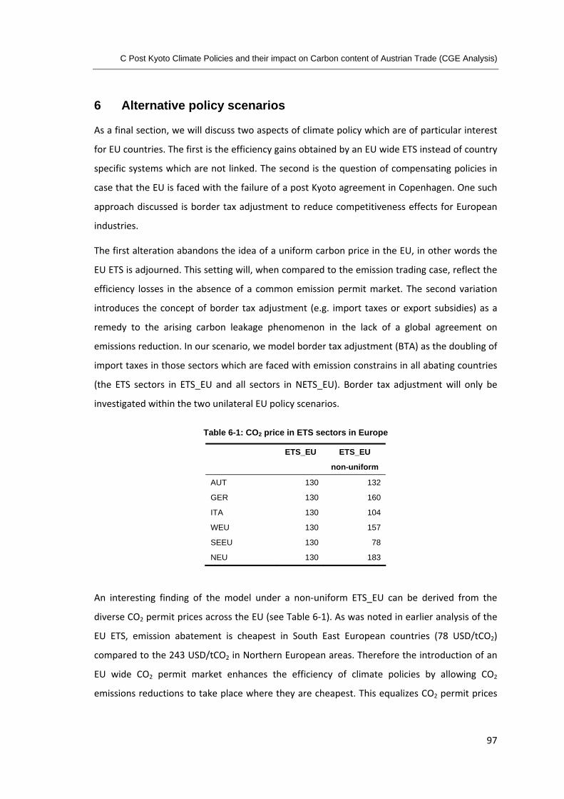
C Post Kyoto Climate Policies and their impact on Carbon content of Austrian Trade (CGE Analysis)
97
6 Alternative policy scenarios
As a final section, we will discuss two aspects of climate policy which are of particular interest
for EU countries. The first is the efficiency gains obtained by an EU wide ETS instead of country
specific systems which are not linked. The second is the question of compensating policies in
case that the EU is faced with the failure of a post Kyoto agreement in Copenhagen. One such
approach discussed is border tax adjustment to reduce competitiveness effects for European
industries.
The first alteration abandons the idea of a uniform carbon price in the EU, in other words the
EU ETS is adjourned. This setting will, when compared to the emission trading case, reflect the
efficiency losses in the absence of a common emission permit market. The second variation
introduces the concept of border tax adjustment (e.g. import taxes or export subsidies) as a
remedy to the arising carbon leakage phenomenon in the lack of a global agreement on
emissions reduction. In our scenario, we model border tax adjustment (BTA) as the doubling of
import taxes in those sectors which are faced with emission constrains in all abating countries
(the ETS sectors in ETS_EU and all sectors in NETS_EU). Border tax adjustment will only be
investigated within the two unilateral EU policy scenarios.
Table 6-1: CO2 price in ETS sectors in Europe
ETS_EU ETS_EU
non-uniform
AUT 130 132
GER 130 160
ITA 130 104
WEU 130 157
SEEU 130 78
NEU 130 183
An interesting finding of the model under a non‐uniform ETS_EU can be derived from the
diverse CO2 permit prices across the EU (see Table 6‐1). As was noted in earlier analysis of the
EU ETS, emission abatement is cheapest in South East European countries (78 USD/tCO2)
compared to the 243 USD/tCO2 in Northern European areas. Therefore the introduction of an
EU wide CO2 permit market enhances the efficiency of climate policies by allowing CO2
emissions reductions to take place where they are cheapest. This equalizes CO2 permit prices
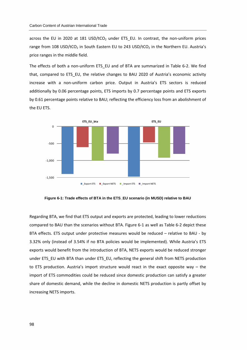
Carbon Content of Austrian International Trade
98
across the EU in 2020 at 181 USD/tCO2 under ETS_EU. In contrast, the non‐uniform prices
range from 108 USD/tCO2 in South Eastern EU to 243 USD/tCO2 in the Northern EU. Austria’s
price ranges in the middle field.
The effects of both a non‐uniform ETS_EU and of BTA are summarized in Table 6‐2. We find
that, compared to ETS_EU, the relative changes to BAU 2020 of Austria’s economic activity
increase with a non‐uniform carbon price. Output in Austria’s ETS sectors is reduced
additionally by 0.06 percentage points, ETS imports by 0.7 percentage points and ETS exports
by 0.61 percentage points relative to BAU; reflecting the efficiency loss from an abolishment of
the EU ETS.
‐1,500
‐1,000
‐500
0
ETS_EU_bta ETS_EU
_Export ETS _Export NETS _Import ETS _Import NETS
Figure 6-1: Trade effects of BTA in the ETS_EU scenario (in MUSD) relative to BAU
Regarding BTA, we find that ETS output and exports are protected, leading to lower reductions
compared to BAU than the scenarios without BTA. Figure 6‐1 as well as Table 6‐2 depict these
BTA effects. ETS output under protective measures would be reduced – relative to BAU ‐ by
3.32% only (instead of 3.54% if no BTA policies would be implemented). While Austria’s ETS
exports would benefit from the introduction of BTA, NETS exports would be reduced stronger
under ETS_EU with BTA than under ETS_EU, reflecting the general shift from NETS production
to ETS production. Austria’s import structure would react in the exact opposite way – the
import of ETS commodities could be reduced since domestic production can satisfy a greater
share of domestic demand, while the decline in domestic NETS production is partly offset by
increasing NETS imports.

C Post Kyoto Climate Policies and their impact on Carbon content of Austrian Trade (CGE Analysis)
99
Table 6-2: Output and trade effects of BTA and a non-uniform carbon price for Austria
BAU 2020 ETS_EU ETS_EU ETS_EU NETS_EU NETS_EU with BTA non-uniform with BTA
in MUSD change relative to BAU 2020 (in %)
GDP
Consumption 247,414 -0.37% -0.36% -0.39% -0.86% -0.84%
Investment 101,964 -0.35% -0.36% -0.34% -0.70% -0.72%
Government 78,793 -0.37% -0.36% -0.39% -0.86% -0.84%
Trade balance -14,843 +1.35% +1.37% +1.06% +20.96% +21.52%
total 413,328 -0.43% -0.42% -0.43% -1.60% -1.61%
growth rate 2.19 2.16 2.16 2.16 2.09 2.08
Output
ETS total 83,621 -3.54% -3.32% -3.60% -5.58% -5.58%
non-ETS total 702,401 -0.38% -0.40% -0.39% -1.64% -1.62%
Output total 786,022 -0.71% -0.71% -0.73% -2.06% -2.04%
Export
ETS total 33,684 -4.38% -4.15% -4.99% -6.09% -6.44%
non-ETS total 137,689 -0.34% -0.44% -0.31% -3.21% -3.65%
Export TRANS 10,343 -0.14% -0.29% -0.07% -8.12% -9.32%
Export total 171,249 +4.97% +4.92% +4.88% +1.85% +1.35%
Import
ETS total 36,654 -2.50% -2.73% -3.20% -4.73% -4.99%
non-ETS total 156,249 -0.52% -0.51% -0.49% -1.51% -1.91%
Import TMG 3,656 -0.82% -0.95% -0.72% -2.88% -4.40%
Import total 196,558 -0.89% -0.93% -1.00% -2.13% -2.53%
For emissions linked to Austrian output and consumption, however, the effects of doubling
import taxes on ETS goods from ROW to the EU are almost negligible. As can be seen from
Table 6‐3, CO2 emissions in Austrian ETS production decrease by 0.05 percentage points less
(compared to BAU) than in ETS_EU. In combination with a slightly stronger CO2 emission
reduction (by 0.02 percentage points) in the NETS sectors compared to ETS_EU – as mentioned
earlier due to decreasing output quantities – Austria’s domestic output related CO2 emissions
are almost not affected by the BTA policy.
By analyzing the BTA effects on Austria’s trade related CO2 emissions in Table 6‐3 and Figure
6‐2, it follows that CO2 emissions embodied in Austria’s exports are subject to a negligible
decrease – by 0.02 percentage points compared to ETS_EU without BTA measures. The slightly
increasing exported ETS emissions compared to ETS_EU are counterbalanced by the
diminishing non‐ETS emissions as well as diminishing emissions delivered to the global
transport market (TRANS), indicated in Austria’s CO2 emission balance (Table 6‐3). For

Carbon Content of Austrian International Trade
100
emissions embodied in Austrian imports, the extra emission reduction of protective measures
can mainly be attributed to decreasing CO2 imports connected to ETS commodities.
Table 6-3: CO2 effects of BTA and a non-uniform carbon price for Austria
BAU 2020 ETS_EU ETS_EU ETS_EU NETS_EU NETS_EU Mt CO2 with BTA unilateral with BTA
change relative to BAU 2020 (in %)
CO2 PrivHH 23.34 +3.79% +3.87% +3.97% -24.30% -24.16%
CO2 Output 67.43 -12.12% -12.10% -12.21% -28.87% -28.92%
PBP 90.77 -8.03% -8.00% -8.05% -27.69% -27.69%
CO2 IM-EX 9.16 -13.84% -14.81% -12.59% +28.12% +28.74%
CBP 99.93 -8.56% -8.62% -8.47% -22.58% -22.52%
CO2 Output
ETS total 32.42 -22.99% -22.94% -23.20% -23.20% -23.20%
non-ETS total 35.01 -2.05% -2.07% -2.03% -34.11% -34.21%
total 67.43 -12.12% -12.10% -12.21% -28.87% -28.92%
CO2 Exports
ETS total 9.03 -22.28% -22.18% -23.46% -22.12% -22.37%
non-ETS total 8.60 -1.72% -1.79% -1.65% -36.83% -37.18%
CO2 TRANS 4.46 -0.48% -0.60% -0.40% -28.39% -29.24%
total 22.09 -9.87% -9.89% -10.32% -29.11% -29.52%
CO2 Imports
ETS total 15.75 -19.54% -20.18% -19.48% -18.82% -18.79%
non-ETS total 12.56 -2.81% -2.70% -2.79% -4.78% -4.52%
CO2 IM TMG 2.93 -0.60% -0.77% -0.42% -9.86% -12.27%
total 31.25 -11.04% -11.33% -10.98% -12.33% -12.44%
‐4
‐3
‐2
‐1
0
ETS_EU_bta ETS_EU
CO2 EX ETS CO2 EX NETS CO2 IM ETS CO2 IM NETS
Figure 6-2: CO2 effects of BTA in the ETS_EU scenario (in MUSD) relative to BAU

C Post Kyoto Climate Policies and their impact on Carbon content of Austrian Trade (CGE Analysis)
101
Finally, in our analysis of BTA measures it can be concluded that a doubling of import taxes
related to imports from non‐EU regions’ ETS sectors has a quite insignificant effect on the
Austrian economy. While in monetary values a movement of Austrian production and trade
activities in the anticipated way can be observed, favorable CO2 effects from the net carbon
balance of Austrian trade are partly counterbalanced by increasing private household
emissions. Therefore Austria’s emissions measured by the CBP approach can be reduced by
8.62% relative to BAU under ETS_EU with BTA, slightly more than without BTA policies (‐
8.56%).
Table 6-4: Global CO2 effects of BTA (in Mt CO2)
BAU ETS_EU ETS_EU_bta
CO2 emissions
policy regions 5,156. 4,507 4,507
non-policy regions 29,006 29,382 29,380
Total 34,163 33,889 33,887
Change relative to 2020
policy regions -649 -649
non policy regions +375 +373
Total -274 -276
Leakage rate 2020 -57.8% -57.5%
Since the debate on carbon leakage in combination with compensation measures has a strong
global dimension – because it is widely assumed that import tariffs set by the EU on
commodities from regions facing less stringent environmental regulations have in addition to
their positive effects on the EU economy ancillary positive effects on global CO2 emissions –
Table 6‐4 presents the model results for the ETS_EU scenario compared to the same scenario
augmented with the previously described protective policy. While the CO2 emissions in the
policy implementing regions can be hold constant at a level of 4,507 Mt CO2, even though
output in the EU is increasing due to protective measures in the ETS sectors, the CO2 emissions
in non‐abating regions can only be slightly reduced, namely by 2 Mt CO2. Therefore, the carbon
leakage rate in the ETS_EU scenario can be reduced only by 0.3 percentage points. If the quite
substantial trade intervention – a 100% increase of the initial 2004 GTAP7 import tariff values
– is weighed against its negligible effect on global CO2 emissions, the appropriateness of BTA
measures have to be questioned. Thus, one of the claims held by proponents of trade

Carbon Content of Austrian International Trade
102
measures that BTA reduces carbon leakage cannot be confirmed within our current model
strucuture. To derive necessary characteristics of BTA to ensure their effectiveness, would
need further investigation which is however beyond the scope of this report.

C Post Kyoto Climate Policies and their impact on Carbon content of Austrian Trade (CGE Analysis)
103
7 Conclusions
Within our CGE model of the Austrian economy and its main trading partners, we analyzed the
consequences of three types of climate policy scenarios relative to a business as usual (BAU)
scenario for 2020, namely two unilateral EU climate policies, analytically separating a policy for
the ETS sectors only (ETS_EU) or also non‐ETS sectors and households (NETS_EU); a voluntary
post Kyoto agreement of Annex I countries (PK_L, PK_H); and a compulsory global agreement
for Annex I countries, with reduction targets as identified by the IPCC’s 4th Assessment Report
to reach the +2° temperature target by 2100 (IPCC_L, IPCC_H). Our main findings can be
summarized as follows.
The BAU 2020: Austrian consumption based carbon emissions almost 40% higher than in
2004
Under BAU 2020, Austrian GDP grows annually at 2.2% (on average for the period 2004 to
2020) and output grows by 30%, predominantly in the non‐ETS sectors. Total imports increase
36% while total exports only increase by 27%, causing Austria’s trade balance to worsen by 13
MUSD (compared to 2004). Austria’s main trading partners are to be found within the EU –
mainly with neighboring countries Germany and Italy; outside the EU the US and Russia are the
strongest single country trading partners.
Austria’s CO2 emissions according to the PBP (production based principle) increase by 14.8%
from 2004 (79 Mt CO2) to 2020 (91 Mt CO2), with a considerably stronger increase by
households than in production. According to the CBP (consumption based principle), Austria’s
emissions increase from 87 Mt CO2 in 2004 by 15% to 100 Mt CO2 in 2020, which is due to a
higher increase in emissions from imports than from exports. As a result, the CO2 trade deficit
of Austria increases by 15% relative to 2004, despite a much stronger increase in Austria’s
trade deficit which increases almost eightfold. This decoupling of emissions from trade flows
reflects on the one hand a global increase in energy efficiency in all production processes and
on the other a shift in the composition of imports from carbon intensive goods (EIS sectors) to
low‐carbon products (NEIS and SERV sectors). Finally, more than 50% of Austria’s CO2
emissions linked to production activities both in 2004 and 2020 arise within ETS sectors –
mainly EIS and ELY – even though the monetary output value of the NETS sectors –
predominantly the NEIS and SERV sectors – is almost nine times higher than the ETS output.

Carbon Content of Austrian International Trade
104
Both unilateral EU and internationally coordinated climate policies affect Austrian
international trade stronger than its domestic production
In scenario ETS_EU, the European Union implements an emissions trading scheme in the
energy intensive sectors (ETS sectors, namely P_C, ELY, EIS) only, but the other countries do
not limit their emissions. This leads to a reduction in Austrian GDP by 0.4% relative to BAU, and
Austrian exports and imports decline by 1.1% and 0.9% respectively. When the European
Union extends its climate policy also to the non‐ETS sectors and households but the other
Annex I countries still do not reduce their emissions, effects on GDP, exports and imports are
more than doubled. The post Kyoto scenarios PK_L and PK_H with voluntary reduction
commitments also by other Annex I countries, further intensify the economic consequences
for GDP, exports, and imports. Finally, under the IPCC emission reduction scenarios which
constitute, according to the IPCC Fourth Assessment Report, the necessary reduction targets
for Annex I countries to remain within the +2° temperature target (compared to pre‐industrial
levels) by 2100, GDP is up to 8.0% lower than under BAU and exports and imports fall by up to
12.5% and 8.6% respectively. Thus, under all scenarios Austrian international trade is affected
more strongly than its domestic production.
At the sectoral level, Austrian production in ETS sectors is hit relatively hard under the
unilateral EU policies, while the non‐ETS sectors are affected more strongly under the
internationally coordinated scenarios (post Kyoto and IPCC). For Austrian exports, a similar
pattern emerges as for its production; moreover, ETS exports to North America and Eastern
Europe are highest under the IPCC scenarios, since the US and Russia are subject to much
more stringent emission targets than under all other scenarios. Austrian imports are slightly
less affected than its exports. Due to the higher openness to trade of the ETS sectors, ETS
imports are affected more strongly than non‐ETS imports. Since Austria’s main trading
partners are within the EU, reductions in imports from the EU are the result of binding
emission targets for all member states. When the EU implements a unilateral policy, imports
from all other regions increase relative to BAU, and particularly so in the ETS sector. In
contrast, when other Annex I countries are faced with binding reduction targets too, Austrian
imports from that regions are lower than under BAU.

C Post Kyoto Climate Policies and their impact on Carbon content of Austrian Trade (CGE Analysis)
105
Austria can achieve the EU 20‐20 emission reduction targets, but its carbon trade balance
worsens considerably
Under all scenarios, Austrian carbon emissions are considerably lower than under BAU 2020,
ranging according to the production based principle (PBP) from 8.0% under ETS_EU to 51.8%
under BAU. These emission reductions are sufficient to reach the EU 20‐20 targets, except for
ETS_EU where the non‐ETS sectors and the households are not committed to reduction
targets. However, the carbon trade balance (emission from export minus emissions from
import) worsens – emissions from Austrian exports decline more than emissions from its
imports, due to a shift in trade partners and a shift from imports of ETS to non‐ETS
commodities. It is striking, that the emissions embodied in imported non‐ETS commodities
hardly respond to the different climate policies while the CO2 emissions linked to ETS
commodities change considerably. Thus, while emissions according to the consumption based
principle (CBP) are lower in all scenarios than under BAU, the reduction is considerably smaller
than according to the PBP since domestic emission reductions are partly offset by increased
emissions from imports.
To achieve a stabilization of global CO2 emissions, a global agreement including non‐Annex I
countries is needed
At the global scale, effects on GDP depend on how universal emission targets are set, both in
terms of sectoral and regional coverage. In both unilateral EU policy scenarios, hardly any GDP
effects arise for regions and countries outside the EU. When all Annex I regions face
constraints, also GDP growth rates of the US and Oceania decline. Regarding worldwide CO2
emissions, the BAU scenario is characterized by 34.2 Gt CO2, already adjusted for economic
slowdown due to the current economic crisis, compared to 27.7 Gt CO2 in 2004.
When the EU introduces binding targets for ETS and non‐ETS sectors and households but all
other countries do not commit themselves, only 1/6th of global emissions are regulated (= EU
20‐20 target) and global emissions still rise by 5.8Gt CO2 above 2004 levels. Even under the
more stringent post Kyoto (PK_L and PK_H) and the IPCC_L scenarios global emissions cannot
be reduced under 2004 levels: emissions increase by 0.9 Gt CO2 to 2.7 Gt CO2 compared to
2004, since Annex I countries only comprise slightly more than 50% of global emissions
(according to the PBP). Only in the most stringent policy scenario that we analyzed within this
paper – IPCC_H, where Annex I countries are constrained to reduce their CO2 emissions by 40%

Carbon Content of Austrian International Trade
106
compared to 1990 levels by 2020 – global CO2 emissions can be mitigated strong enough to fall
by 1 Gt CO2 under the 2004 level (which was at 27.7 Gt CO2).
Carbon leakage from non‐abating to abating regions occurs in all scenarios, ranging from 58%
(EU_ETS) to 21% (IPCC_H). Thus, the more countries, and in particular other major economies
like the US (and the rest of North America), Russia and Oceania, commit themselves to binding
emission targets, the lower the rate of leakage and the less carbon intensive are domestic
production and the imports from those countries. This argument can be extended to non‐
Annex I countries: in a post Kyoto agreement, developing countries, in particular China, have
to play a substantial role to halt carbon leakage and to thereby achieve a stabilization of
carbon emissions on a global scale.

C Post Kyoto Climate Policies and their impact on Carbon content of Austrian Trade (CGE Analysis)
107
8 References
Armington, P. (1969). “A theory of demand for products distinguished by place of production”. IMF staff papers, 16, 1969, 159‐178.
Beckman, J.F. and T.W. Hertel (2009). “Why Previous Estimates of the Cost of Climate Mitigation are Likely Too Low.” GTAP Working Paper No.54, Purdue University.
Böhringer, C. (1999). PACE – Policy Assessment based on Computable Equilibrium. Ein flexiblles Modellsystem zur gesamtwirtschaftlichen Analyse von wirtschaftspolitischen Maßnahmen. ZEW Dokumentation, Centre for European Economic Research. Mannheim, Germany.
Burniaux, J.M., J.P. Martin, G. Nicoletti and J. Oliveira (1992). GREEN – A Multi‐Regional Dynamic General Equilibrium Model for Quantifying the Costs of Curbing CO2 Emissions: A Technical Manual. Working Paper 116, Economics and Statistics Department, OECD, Paris.
Centre for Global Trade Analysis, Purdue University (2007). Global Trade, Assistance and Production: The GTAP 7 Data Base. West Lafayette.
European Commission (2008). “20 20 by 2020. Europe’s climate change opportunity.” Communication from the European Commission to the European Parliament, the council, the European economic and social committee and the committee of the regions. Brussels.
European Parliament (2003). “Directive 2003/87/EC of the European Parliament and the Council. Establishing a Scheme for Greenhouse Gas Emissions Allowance Trading within the Community and amending Council Directive 96/61/EC.” Brussels.
Fisher, B.S., N. Nakicenovic, K. Alfsen, J. Corfee Morlot, F. de la Chesnaye, J.‐Ch. Hourcade, K. Jiang, M. Kainuma, E. La Rovere, A. Matysek, A. Rana, K. Riahi, R. Richels, S. Rose, D. van Vuuren, R. Warren, 2007: Issues related to mitigation in the long term context, In Climate Change 2007: Mitigation. Contribution of Working Group III to the Fourth Assessment Report of the Inter‐governmental Panel on Climate Change [B. Metz, O.R. Davidson, P.R. Bosch, R. Dave, L.A. Meyer (eds)], Cambridge University Press, Cambridge,
Grossmann, W., K. Steininger, I. Grossmann, L. Magaard (2009), Indicators on Economic Risk from Global Climate Change, Environmental Science and Technology 43(16): 6421‐6426.
Helm, D., R. Smale and J. Phillips (2007). "Too Good To Be True? The UK’s Climate Change Record." http://www.vivideconomics.com/portfolio.html.
Peters, G., E. Hertwich (2008). CO Embodied in International Trade with Implications for Global Climate Policy. Environmental Science Technology; 42(5) 1401‐1407.
IMF (2009). World economic and financial surveys. World economic outlook database. International Monetary Fund. Available at: http://www.imf.org/external/pubs/ft/weo/2009/02/weodata/download.aspx.
IPCC (2007). 4th Assessment report, Climate Change 2007: Synthesis report, Intergovernmental Panel on Climate Change. Cambridge, Cambridge University Press.
Lee, H.‐L. (2008). The Combustion‐based CO2 Emissions Data for GTAP Version 7 Data Base. Department of Economics, National Chengchi University, Taiwan. Available at: https://www.gtap.agecon.purdue.edu/resources/res_display.asp?RecordID=1143.
Lenzen, M., J. Murray, F. Sack, T. Wiedmann (2007). Shared producer and consumer responsibility — Theory and practice. Ecological Economics. 61(1), 27‐42.
Lenzen, M., L.L. Pade and J. Munksgaard (2004). CO2 multipliers in multi‐region input‐output models. Economic Systems Research; 16(4) 391–412.

Carbon Content of Austrian International Trade
108
Meinshausen, M, N. Meinshausen, W. Hare, S.C. B. Raper, K. Frieler, R. Knutti, D.J. Frame, M,R. Allen (2009). Greenhouse‐gas emission targets for limiting global warming to 20C, Nature Vol 485 , April 30, doi 10.1038/nature08017.
Munksgaard, J., K. Pedersen (2001). CO2 accounts for open economies: producer or consumer responsibility. Energy Policy, 29 327–334.
Okagawa, A. and Ban, K. (2008), Discussion Paper 08—16: Estimation of Substitution Elasticities for CGE Models, Graduate School of Economics and Osaka School of International Public Policy (OSIPP) Osaka University, Toyonaka, Osaka 560‐0043, Japan.
Poncet, S. (2006). The Long Term Growth Prospects of the World Economy: Horizon 2050. Working Paper 2006–16. Centre d’Etudes Prospectives et d’Informations Internationales.
McDougall, R. And H.‐L. Lee (2006). “An energy data base for GTAP.” In Global Trade, Assistance and Production: The GTAP 6 Data Base, chapter 17. Center for Global Trade Analysis, Purdue University.
McDougall, R. and A. Aguiar (2007). “Initial Preparation of Energy Volume Data for GTAP 7.” GTAP Research Memorandum No. 10. Center for Global Trade Analysis, Purdue University.
Rutherford, T.F. (1999). Applied General Equlibrium Modeling with MPSGE as a GAMS Subsystem: AN overview of the modeling framework and syntax. Computational Economics, 14 (1‐2)
Rutherford, T.F. and S.V. Paltsev (2000). “GTAP‐Energy in GAMS.” University of Colorado, Working Paper 00‐2 2000. http://debreu.colorado.edu/download/gtap‐eg.pdf.
Steininger, K., S. Schleicher, B. Gebetsroither, T. Schinko, A. Tuerk (2009). Klimaschutzplan Steiermark, Teilbericht 1: Emissionen, Sektorale Zurechung und EU 2020 Ziele.
UMWELTBUNDESAMT (2008): Muik, B.; Anderl, M.; Freudenschuß, A.; Kampel, E.; Köther, T.; Poupa, S.;Schodl, B.; Schwaiger, E.; Seuss, K.; Weiss, P.; Wieser, M.; Winiwarter, W. & Zethner, G.: Austria’s National Inventory Report 2008. Submission under the United Nations Framework Convention on Climate Change. Reports, Bd. REP‐0152. Umweltbundesamt, Wien.
UNFCCC(2009).” http://unfccc.int/ghg_data/items/3800.php.” United Framework Convention on Climate Change.
Wiedmann T, M. Lenzen, K. Turner, J. Barrett (2007). Examining the global environmental impact of regional consumption activities — Part 2: Review of input–output models for the assessment of environmental impacts embodied in trade. Ecological Economics; 61(1) 15‐26.