The Cartographic Representation of Language: Understanding language map construction and visualizing language diversity

Candice Rae Luebbering

Dissertation submitted to the faculty of the Virginia Polytechnic Institute and State University in partial fulfillment of the requirements for the degree of

Doctor of Philosophy In

Geospatial and Environmental Analysis

Korine N. Kolivras (Co-chair) Stephen P. Prisley (Co-chair) Laurence W. Carstensen Jr.

Lynn M. Resler

March 23, 2011 Blacksburg, VA

Keywords: cartography, GIS, language, linguistics, map design

Copyright 2011, Candice R. Luebbering

The Cartographic Presentation of Language: Understanding language map construction and visualizing language diversity

Candice Rae Luebbering

ABSTRACT

Language maps provide illustrations of linguistic and cultural diversity and distribution, appearing in outlets ranging from textbooks and news articles to websites and wall maps. They are valuable visual aids that accompany discussions of our cultural climate. Despite the prevalent use of language maps as educational tools, little recent research addresses the difficult task of map construction for this fluid cultural characteristic. The display and analysis capabilities of current geographic information systems (GIS) provide a new opportunity for revisiting and challenging the issues of language mapping. In an effort to renew language mapping research and explore the potential of GIS, this dissertation is composed of three studies that collectively present a progressive work on language mapping. The first study summarizes the language mapping literature, addressing the difficulties and limitations of assigning language to space before describing contemporary language mapping projects as well as future research possibilities with current technology. In an effort to identify common language mapping practices, the second study is a map survey documenting the cartographic characteristics of existing language maps. The survey not only consistently categorizes language map symbology, it also captures unique strategies observed for handling locations with linguistic plurality as well as representing language data uncertainty. A new typology of language map symbology is compiled based on the map survey results. Finally, the third study specifically addresses two gaps in the language mapping literature: the issue of visualizing linguistic diversity and the scarcity of GIS applications in language mapping research. The study uses census data for the Washington, D.C. Metropolitan Statistical Area to explore visualization possibilities for representing the linguistic diversity. After recreating mapping strategies already in use for showing linguistic diversity, the study applies an existing statistic (a linguistic diversity index) as a new mapping variable to generate a new visualization type: a linguistic diversity surface. The overall goal of this dissertation is to provide the impetus for continued language mapping research and contribute to the understanding and creation of language maps in education, research, politics, and other venues.

iii

Acknowledgements

As anyone who has carried the label ‘grad student’ knows, the graduate school experience is a life of constant emotional (and research) ups and downs. I would simply like to acknowledge everyone who at some point along my path joined me in celebrating the ups or helped encourage me through the downs. I would like to specifically acknowledge the following: The Department of Geography faculty: Thank you for tolerating my presence throughout my masters and PhD. I have enjoyed getting to know each one of you and appreciate the insight and humor you have shared with me over the years. My fellow geography grad students: I’ll miss being part of our always dysfunctional yet always entertaining pack of diverse personalities. You are the foundation of Major Bill (literally – as the most frequent dwellers of its lowest floor)! And most importantly….if I can do it, so can you! My dog Ala-Mo: My little Boston Terrier served as a 13lb. stress relief ball. A good cuddle with her at the end of a long day melted all frustrations away. Upon submitting this dissertation you have earned a long streak of days at the dog park and laying in the sun. My co-chairs: I consider myself extremely lucky to have found a perfect combination of professional and personal support from you two. Steve – your unrelenting enthusiasm for my topic and ideas helped me to become a believer in my own work. Korine – I don’t think anyone else could have kept me in line and understood me as well as you did. Thanks for all of your time, your stories, and for redefining the word “fun”. My parents: The most supporting and influential duo in my life – you always make me feel special, brilliant, and loved. I am always proud to do you proud and am a PhD because you said I could be. My husband: You had to take the brunt of my grad school frustrations. Despite my many crazy days, your patient soul was (and is) always my most solid and consistent source of encouragement, support, laughter, and love. Had it not been for graduate school, I never would have met you. Had it not been for you, I never would have made it through graduate school.

iv

Table of Contents

Abstract........................................................................................................................................ ii Acknowledgements ....................................................................................................................iii List of Tables .............................................................................................................................. vi List of Figures............................................................................................................................vii Chapter 1: Introduction ............................................................................................................ 1 1. Research Context and Justification.............................................................................. 1 2. Dissertation Components and Research Questions...................................................... 3 3. References.................................................................................................................... 5 Chapter 2: Displaying the geography of language: the cartography of language maps ..... 8 Abstract ............................................................................................................................. 8 1. Introduction.................................................................................................................. 8 2. Geolinguistics ............................................................................................................ 10 3. Language Mapping .................................................................................................... 11 4. Problems with Language Mapping ............................................................................ 14 4.1. Scale.................................................................................................................. 14 4.2. Vector Format ................................................................................................... 15 4.2.1. Boundary Issues ....................................................................................... 15 4.2.2. Map Units................................................................................................. 16 4.2.3. Power and Perception .............................................................................. 17 5. Computerization and the Potential of GIS for Language Mapping ........................... 18 6. Current Language Projects using GIS and/or the Internet ......................................... 19 7. Future Research ......................................................................................................... 22 8. References.................................................................................................................. 25

Chapter 3: The Lay of the Language: Surveying the cartographic characteristics of language maps ........................................................................................................................... 37 Abstract ........................................................................................................................... 37 1. Introduction................................................................................................................ 37 2. Related Work ............................................................................................................. 39 3. Methods...................................................................................................................... 44 3.1. Collection of Map Sample ................................................................................ 44 3.2. Language Map Sample Limitations .................................................................. 45 3.3. Survey Components, Map Classification Typology, and Data Collection and Analysis............................................................................................................. 46 4. Results........................................................................................................................ 48 4.1. Basic Map Sample and Design Characteristics ................................................ 48 4.2. Language Map Design Elements and Construction Issues ............................... 48 4.3. Application of Ambrose & Williams’ (1991) Symbology Types..................... 50 4.4. Unique Strategies Observed.............................................................................. 50

v

5. Discussion .................................................................................................................. 51 6. Updating Ambrose and Williams’ Typology............................................................. 58 7. Summary and Conclusions ........................................................................................ 60 8. References.................................................................................................................. 62

Chapter 4: Visualizing Linguistic Diversity through Cartography and GIS: A case study of commonly used techniques and the potential of linguistic diversity index mapping.......... 82 Abstract ........................................................................................................................... 82 1. Introduction................................................................................................................ 82 2. Related Work ............................................................................................................. 85 2.1. Difficulties and Limitations of Current Language Mapping Practices............. 85 2.2. Power and Perception in Language Mapping ................................................... 87 2.3. Quality of Census Data on Language ............................................................... 87 2.4. Language Map Production and Analysis with GIS........................................... 88 3. Language and Base Map Data ................................................................................... 89 3.1. Language Dataset.............................................................................................. 89 3.2. Study Area and Base Map Files........................................................................ 90 4. Case Study of Visualization of Linguistic Diversity ................................................. 90 4.1. Leading Languages after English...................................................................... 91 4.2. Percentage of Individual Language Speakers ................................................... 92 4.3. Percentage of Speakers of all Non-majority Languages................................... 93 4.4. Pie Chart Symbology ........................................................................................ 94 4.5. Dot Density Map............................................................................................... 95 5. Mapping with Linguistic Diversity Indices ............................................................... 97 5.1. Methods for Calculating Linguistic Diversity Indices...................................... 98 5.2. Linguistic Diversity Index Map – Vector Format............................................. 99 5.3. Linguistic Diversity Index Map – Raster Format ........................................... 102 6. Conclusions and Future Research............................................................................ 103 7. References................................................................................................................ 106 Chapter 5: Conclusion ........................................................................................................... 123 1. Conclusions.............................................................................................................. 123 2. References................................................................................................................ 128 Appendix A: Language Map Survey Sheet ......................................................................... 129

vi

List of Tables Table 2.1. List of language mapping projects available online with project descriptions and URLs......................................................................................................................... 36 Table 3.1. Frequency of coverage extents used in the map sample. ......................................... 76 Table 3.2. Use of points, lines, and polygons for language data depiction............................... 76 Table 3.3. Generalized language variable types and frequency of use within the map sample ....................................................................................................................... 77 Table 3.4. Use of solid versus non-solid boundary lines for language items on maps ............. 78 Table 3.5. Most common map unit categories and use of political map units observed in the sample ....................................................................................................................... 78 Table 3.6. Number of language items and language items per place observed in the map sample ....................................................................................................................... 79 Table 3.7. Use of Ambrose & Williams’ symbology types and the top symbology types overall (combinations included). .......................................................................................... 79 Table 3.8. Sample of map caveat quotes observed. .................................................................. 80 Table 3.9: Use of new typology symbology types and the top symbology types overall (combinations included). .......................................................................................... 81

vii

List of Figures Figure 1.1. World language map found in a human geography textbook.................................... 7 Figure 2.1. Example of a world language map in a human geography textbook....................... 31 Figure 2.2. Ambrose and Williams (1991) diagram showing common language mapping symbols ..................................................................................................................... 32 Figure 2.3. Example of isogloss map and isogloss bunching. .................................................. 33 Figure 2.4. Example of early computerized language map........................................................ 34 Figure 2.5. Example of a GIS generated map from VGI data on the different terms used for soft drinks in the US ........................................................................................................ 35 Figure 3.1. World language map figure in a textbook for introductory human geography ....... 67 Figure 3.2. Ambrose and Williams (1991) diagram showing common language mapping symbols ..................................................................................................................... 68 Figure 3.3. Distribution of source types for the map sample..................................................... 69 Figure 3.4. Distribution of publication decades for maps and map sources (7 websites without dates excluded) ......................................................................................................... 70 Figure 3.5. Use of non-solid line boundaries for visual distinction, not to indicate uncertainty or fluidity of data........................................................................................................... 71 Figure 3.6. Map symbology strategies observed for visualizing multilingualism.................... 72 Figure 3.7. Unique examples of language map uncertainty and boundary depiction................ 73 Figure 3.8. Examples of unanchored or floating language labels............................................. 74 Figure 3.9. Updated Ambrose and Williams’ (1991) typology of language mapping symbology types based on map survey observations .................................................................. 75 Figure 4.1. Study area map of Washington, D. C. Metropolitan Statistical Area................... 111 Figure 4.2. Leading language category after English by census tract in the Washington, D.C. Metropolitan Statistical Area.................................................................................. 112 Figure 4.3. Percentage of population that speaks Spanish by census tract in the Washington, D.C. Metropolitan Statistical Area ......................................................................... 113

viii

Figure 4.4. Percentage of population that speaks any language other than English by census tract in the Washington, D.C. Metropolitan Statistical Area .......................................... 114 Figure 4.5. Map series showing the percentage of population, by census tract, that speaks the top ten most prevalent languages after English in the Washington, D. C. Metropolitan Statistical Area........................................................................................................ 115 Figure 4.6. Dot density maps of A) English speakers and B) Spanish speakers in the Washington, D.C. Metropolitan Statistical Area .................................................... 116 Figure 4.7. Dot density maps of A) languages with > 100 speakers (excluding English and Spanish) and B) languages with < 1000 speakers in the Washington, D. C. Metropolitan Statistical Area.................................................................................. 117 Figure 4.8. Vector map of linguistic diversity index values by census tract in the Washington, D.C. Metropolitan Statistical Area ......................................................................... 118 Figure 4.9. Previous linguistic surfaces research by A) Wikle (1997) and B) Taylor (1977)...................................................................................................................... 119 Figure 4.10. 3-dimensional vector models of linguistic diversity index values by census tract in the Washington, D.C. Metropolitan Statistical Area .............................................. 120 Figure 4.11. Raster maps of linguistic diversity index values by census tract for the Washington, D.C. Metropolitan Statistical Area ......................................................................... 121 Figure 4.12. 3-dimensional raster models of linguistic diversity index values by census tract in the Washington, D.C. Metropolitan Statistical Area .............................................. 122

1

Chapter 1: Introduction

1. Research Context and Justification

My grandparents spoke German, my in-laws speak Hindi and Tagalog, and I often have

to choose among language options for websites, at ATMs, or on automated phone help-lines.

Although I am a monolingual English-speaking American citizen, my life experiences include

many indications of the presence of other languages. Linguistic diversity is on the rise in the

United States and our current cultural climate is constantly changing. Grasping the concepts of

linguistic and cultural diversity is an important lesson for students today and a staple component

of most college-level introductory human or cultural geography courses. Accompanying these

lessons are figures of language maps showing the spatial distribution of dialects, languages, or

language families (e.g. Fouberg, Murphy, and de Blij 2009; Dahlman, Renwick, and Bergman

2010; Getis et al. 2010; Knox and Marston 2010; Marston et al. 2010; Rubenstein 2010). While

such maps provide welcome visual aids that assist students in understanding the varying

distribution of different tongues and cultures, closer inspection may provide more questions than

answers (Figure 1.1). The data and design decisions made to compile language maps can

undermine their utility if the end product disguises more about language than it reveals. Often

these educational figures remain relatively unchanged through subsequent textbook editions

despite the ongoing linguistic change in the world and the outdated or even flawed depictions in

the maps. As a geography student pondering Figure 1.1, I am left questioning the conflict of the

labels “indigenous languages” and “major languages” that are used interchangeably while also

well aware that my life experiences with language are not visible on the map. Language maps

also have applicability beyond the educational realm such as in political discussions related to

immigration (e.g. English-only movements in the U.S.), emergency services, and marketing

among other possibilities. Knowing who speaks what and where is important, if not critical, for

many applications and thus language maps and language mapping have the potential for

widespread utility.

Language mapping is not a simple task. While determining and depicting the location

and extent of any feature requires considerable knowledge and skill, the fluidity and intangibility

of language make it an extremely difficult map subject. In addressing the ability or inability to

reflect the reality of language on a map, we are revisiting a widely held basic cartographic tenet

2

of the map as a communication system (Robinson and Petchenik 1976). Maps represent a

communication process with information passing from reality through the different filters of the

cartographer and map user (MacEachren 1995). Keeping in mind the intended purpose of the

map, the cartographer should strive to use symbology and design characteristics that are most

appropriate for conveying the content (Robinson 1952). In the case of language mapping, this

translates into the difficult task of finding conventional symbology that can appropriately

represent the complexity of language or at the very least appropriately represent the aspect of

language related to the map’s purpose.

There are language maps dating as early as the 1700s (Lameli 2010) with large,

systematic linguistic atlas projects carried out in the late 1800s (Crystal 1997); however, this

long history of language mapping has not reduced the difficulty of the job. The linguistic

environment has become more complex as populations have migrated and intermingled, but what

is more problematic is that language mapping still lacks what many other traditions have in

place: guidelines. There are no established guidelines, rules, or standards for language mapping

(Kirk, Sanderson, and Widdowson 1985; Ambrose and Williams 1991; Williams 1996). Instead,

the literature provides thorough discussion of the woes of language map construction, many due

to the limitations of a vector environment of points, lines, and polygons, for capturing a fluid,

continuous phenomenon such as language (Breton 1991). Major language mapping issues

include map unit choice (specifically the frequent employment of political map units) (Ambrose

and Williams 1991; Ormeling 1992; Williams 1996), boundary depiction (Kirk, Sanderson, and

Widdowson 1985; Macaulay 1985; Mackey 1988; Williams and Ambrose 1988; Ormeling 1992;

Williams 1996; Davis 2000), and the battle of power and perception (whose language will be

represented on the map, whose will not) (Breton 1992; Peeters 1992; Williams and Ambrose

1992; Williams 1996). A language map is a mere representation of reality but the extent of

compromises that are made to depict the fluidity of language within the discrete confines of a

map can result in a product that is far from reality not only in the location of features, but in the

messages conveyed about the characteristics of language itself.

With most of the pertinent language mapping literature well over a decade old, the

question remains whether a contemporary approach to the task might produce new possible

solutions to old language mapping problems. The potential of geographic information systems

(GIS), among other new geospatial tools, is touted for language data display and analysis

3

(Williams and Ambrose 1992; Lee and Kretzschmar 1993; Williams 1996; Williams and Van der

Merwe 1996; Kretzschmar 1997), yet geolinguistic research features very little work with GIS

(Hoch and Hayes 2010). The research presented in this dissertation seeks to renew attention to

the issue of language mapping and begin to address the capability of contemporary mapping

technology to produce improved language mapping products. Language mapping’s long history

and progression is continued with the aim of maintaining language maps’ relevancy and utility in

modern society. Students are increasingly becoming global citizens living global lives; language

maps, when carefully considered and constructed, can assist in teaching important lessons to

these up-and-coming members of our global society.

2. Dissertation Components and Research Questions

This dissertation is composed of three manuscript chapters prepared for submission to

peer-reviewed academic journals. Each manuscript chapter builds upon the previous one to

present a progressive study of language mapping that summarizes language mapping history and

practice, documents language map characteristics, and explores visualizing language diversity.

The first manuscript (Chapter 2) is a literature review paper that provides the foundation for this

dissertation as a whole and presents language mapping to a new audience of today’s scholars.

Three research questions are pursued in this chapter: 1) what are the difficulties and limitations

of assigning language to space, 2) what current language mapping projects are taking place, and,

3) what opportunities are there for improving language mapping with current technology.

Building from the literature, the second manuscript (Chapter 3) addresses the absence of

language mapping guidelines. This manuscript is the first work to systematically survey

language map characteristics and quantify the patterns of language mapping in practice as a

means for understanding both the most common and unique strategies used for cartographically

representing language. The survey research asks two research questions: 1) what are the

common cartographic characteristics of language maps, and, 2) does the existing general

symbology typology of Ambrose and Williams (1991) adequately capture language mapping in

practice? Finally, the third manuscript (Chapter 4) is a visualization study specifically focused

on the representation of linguistic diversity through different language mapping strategies.

Using GIS to create different maps from the same dataset, we critique the ability of different

current mapping strategies to capture and display linguistic diversity before exploring the

4

potential use of a linguistic diversity index, an existing statistic rarely used as a mapping

variable, for language mapping. Two research questions form the motivation for this work: 1)

can today’s mapping technology produce meaningful representations of linguistic diversity

(rather than language dominance) to serve as educational or research tools, and, 2) are there other

measures available, such as the linguistic diversity index, that could serve as useful language

mapping variables?

Together, these manuscripts present a progressive study of language mapping. This

dissertation assesses the current state and practices of the field before pursuing new research

initiatives and discussing additional future research directions. Each manuscript contributes its

own recommendations for language mapping pursuits and these are summarized in the

conclusion in chapter 5.

5

3. References Ambrose, J. E., and C. H. Williams. 1991. Language Made Visible: Representation in Geolinguistics. In Linguistic Minorities, Society and Territory, ed. C. H. Williams, 298- 314. Clevedon: Multilingual Matters, Ltd. Breton, R. 1991. Geolinguistics: Language dynamics and ethnolinguistic geography. Ottawa: University of Ottawa Press. -----. 1992. 'Easy Geolinguistics' and Cartographers. Discussion Papers in Geolinguistics, 19 – 21: 68-70. Crystal, D. 1997. The Cambridge Encyclopedia of Language. Cambridge: Cambridge University Press. Dahlman, C., W. H. Renwick, and E. Bergman. 2010. Introduction to Geography: People, places, and environments. 5th ed. Upper Saddle River, New Jersey: Pearson Prentice Hall. Davis, L. M. 2000. The reliability of dialect boundaries. American Speech 75: 257-259. Fouberg, E. H., A. B. Murphy, and H. J. de Blij. 2009. Human Geography: People, Place, and Culture. 9th ed. US: John Wiley & Sons, Inc. Getis, A., J. Getis, M. Bjelland, and J. D. Fellmann. 2010. Introduction to Geography. 13th ed. New York, NY: McGraw-Hill. Hoch, S., and J. J. Hayes. 2010. Geolinguistics: The incorporation of geographic information

systems and science. The Geographical Bulletin 51: 23-36. Kirk, J. M., S. Sanderson, and J. D. A. Widdowson. 1985. Introduction: Principles and practice

in linguistic geography. In Studies in linguistic geography: The dialects of English in Britain and Ireland, eds. J. M. Kirk, S. Sanderson and J. D. A. Widdowson, 1–33. London: Croom Helm.

Knox, P. L., and S. A. Marston. 2010. Human Geography: Place and Regions in Global

Context, 5th ed. Upper Saddle River, New Jersey: Pearson Prentice Hall. Kretzschmar, W. A., Jr. 1997. Generating linguistic feature maps with statistics. In Language variety in the South revisited, eds. C. Bernstein, T. Nunnally, and R. Sabino, 392-416. Tuscaloosa: University of Alabama Press. Lameli, A. 2010. Linguistic atlases – traditional and modern. In Language and Space: An

international handbook of linguistic variation. Volume 1: Theories and methods, eds. P. Auer and J. E. Schmidt, 567-592. New York: De Gruyter Mouton.

Lee, J., and J. W. A. Kretzschmar. 1993. Spatial analysis of linguistic data with GIS functions.

6

International Journal of Geographical Information Systems 7: 541-560. Macaulay, R. K. S. 1985. Linguistic maps: Visual aid or abstract art? In Studies in linguistic

geography: The dialects of English in Britain and Ireland, eds. J. M. Kirk, S. Sanderson, and J. D. A. Widdowson, 172–186. London: Croom Helm.

MacEachren, A. M. 1995. How Maps Work: Representation,visualization, and design. New York: The Guilford Press. Mackey, W. F. 1988. Geolinguistics: Its scope and principles. In Language in geographic

context, ed. C. H. Williams, 20-46. Philadelphia: Multilingual Matters, Ltd. Marston, S. A., P. L. Knox, D. M. Liverman, V. Del Casino, and P. Robbins 2010. World Regions in Global Context: Peoples, Place and Environments. 4th ed. Upper Saddle River, NJ: Pearson Prentice Hall. Ormeling, F. 1992. Methods and possibilities for mapping by onomasticians. Discussion Papers

in Geolinguistics 19-21: 50-67. Peeters, Y. J. D. 1992. The political importance of the visualisation of language contact.

Discussion Papers in Geolinguistics 19-21: 6-8. Robinson, A. H. 1952. The Look of Maps. Madison, WI: University of Wisconsin Press. Robinson, A. H., and B. B. Petchenik. 1976. The Nature of Maps: Essays toward understanding maps and mapping. Chicago: University of Chicago Press. Rubenstein, J. M. 2010. The Cultural Landscape: An Introduction to Human Geography. 10th ed. Upper Saddle River, NJ: Pearson Prentice Hall. Williams, C. H. 1996. Geography and contact linguistics. In Contact linguistics: An

International Handbook of Contemporary Research, eds. H. Goebl, P. H. Nelde, Z. Stary, and W. Wolck, 63-75. New York: Walter de Gruyter.

Williams, C. H., and J. E. Ambrose. 1988. On measuring language border areas. In Language in

geographic context, ed. C. H. Williams, 93-135. Philadelphia: Multilingual Matters, Ltd. -----. 1992. Geolinguistic Developments and Cartographic Problems. Discussion Papers in

Geolinguistics 19-21: 11-32. Williams, C. H., and I. Van der Merwe. 1996. Mapping the multilingual city: A research agenda

for urban geolinguistics. Journal of Multilingual and Multicultural Development 17: 49-66.

7

Figure 1.1. World language map found in a human geography textbook. The caption reads “major languages and major language families” while the legend states “the world’s indigenous languages.” The source information indicates that the map is compiled from three different sources. The methodologies of these mapping sources are not described. (Image source: Knox and Marston, 2010)

8

Chapter 2: Displaying the geography of language: the cartography of language maps

Abstract:

Language maps are often used as educational tools to provide illustrations of linguistic

and cultural diversity and distribution. Despite the prevalent use of language maps, very little

recent research addresses the problematic task of their construction. Given current GIS capability

and the potential to tackle previous visualization troubles, the fundamental issues of language

mapping are reexamined as a starting point for improving the effectiveness of modern language

maps. This review work addresses the difficulties of assigning language to space, describes

current language mapping projects, and discusses the potential of current technology for

improving language mapping.

Key Words: cartography, GIS, language, linguistics, map design

1. Introduction

While browsing through an introductory textbook for human or cultural geography, it is

common to find a map displaying the world’s major languages or language families. This

simplistic map does not, and does not attempt to, show the true diversity and complexity of the

world’s language environment. However, the purpose of such a generalized map is often unclear

(Figure 2.1). The viewer cannot be certain if the map shows official languages, the languages of

the majority, or perhaps the language of the ruling class. What does a boundary line indicate?

What aspect of language policy or language practice does it represent? By researching these

aspects of data definition and visualization, geographers and cartographers contribute to the

understanding of, and present new ideas for, the spatial representation of language.

Language maps occupy a precarious existence; they are useful and informative, but are

rather problematic to create. They provide illustrations of linguistic and cultural diversity that

serve as educational tools in various disciplines (ex. geography, anthropology, sociology) and at

various educational levels. However, like many cultural phenomena that do not follow the

physical landscape or possess strict environmental constraints, language is fluid and rather

intangible, making it extremely difficult to map. Further, as noted by Mackey (1988), language

is not as attached to space as it once was; in the two subsequent decades since his article, this is

9

only more so the case. The language landscape is constantly changing; at best, language maps

are generalized snapshots in time.

While determining what constitutes a language and distinguishing among languages is

the research of linguists, the map presentation format used for displaying language information is

typically the work of cartographers and geographers. Viewed as a vehicle for communication,

maps are designed with their purpose, audience, and intended meaning in mind (MacEachren,

1995). Maps are not just static images, but rather communication systems with information

passing through the filters of the mapmaker and map user (Robinson and Petchenik, 1976).

Symbology and design choices should relate not just to their visual appeal and coherence, but

also to their appropriateness for conveying the data reality and the map’s intended purpose

(Robinson, 1952). Though many language maps appear to achieve their purpose, there are a

number of conceptual cartographic problems that can cause misrepresentation of a linguistic

environment. First, most language maps are in a vector format made up of points, lines, and

polygons. This discrete mapping method depicts a landscape of sharp divides. However, when

reading about the nature of language, the descriptions are ones of fluidity and a continuous

surface. These are ill-suited characteristics for depiction in a vector world. Also, language maps

often feature only one language per location, conveying the idea of one language per place.

Given the flow of both information and people in the world today, few places are likely to be so

linguistically one-dimensional. Finally, language mapping shares the same problem that the

mapping of many phenomena does: improper map unit choice. Ideally, individuals would serve

as the minimal mapping unit for language. Given the difficulty and ethicality of mapping

individual people however, many language maps use political units such as the country, state, or

county level (or equivalent system). Languages do not necessarily operate or aggregate at these

politically defined scales so use of such boundaries may disguise the real language landscape.

Peeters (1992) states that language maps are inherently controversial, with no single

language map sufficing to satisfy all of its users. In addition, most language maps are found to

be rather boring (Williams and Ambrose, 1992), devoid of much design creativity (Williams,

1996). While this may be the case, language maps continue to be produced as reference and

teaching tools so continued effort should be made towards their understanding and improvement.

Despite the problematic yet important task of generating language maps, very little recent

research addresses this topic. With the advent of geographic information systems (GIS) and

10

improved computing efficiency in general, there are now new opportunities for exploring and

understanding the cartography of language maps. Providing a review of pertinent language

mapping literature along with discussion of new language mapping projects in progress, this

article aims to renew interest in the cartography of language mapping.

Recent works provide general reviews of language mapping (Hoch and Hayes, 2010;

Wikle and Bailey, 2010); these welcome additions to the language mapping literature contribute

different approaches than the general cartographic and visualization focus pursued here. Hoch

and Hayes (2010) provide a summary of some current geolinguistic GIS projects as well as an

excellent discussion of the potential analysis capabilities of GIS for language data; specifically,

they state that GIS is not used as much as it could be for data management and analysis of

linguistic datasets. They provide examples of GIS techniques such as kriging and point pattern

analysis and their potential application for geolinguistic research. Wikle and Bailey (2010) take

a more topical approach, narrowing in on the mapping of English in North America for their

review piece. Through their particular language and regional focus, Wikle and Bailey (2010)

summarize the major events in the history of maps in language research and describe

contemporary projects that map English in North America using GIS and Internet-based

capabilities. In contrast to the analysis focus of Hoch and Hayes (2010) and the topical history

of Wikle and Bailey (2010), this research takes a broad focus to concentrate on the presentation

of language maps, investigating their visual appearance, associated meaning, and the potential of

improving their cartographic composition. This review revives the efforts of geographers in the

1980s and 1990s who brought attention to the problematic aspects of language mapping and

called for efforts to improve language maps, especially those used in educational settings

(Ambrose and Williams, 1989; Ambrose and Williams, 1991; Mackey, 1988; Zelinsky and

Williams, 1985). To begin the process of understanding, evaluating, and improving the

communicability of language maps, this work addresses the difficulties and limitations of

assigning language to space, introduces current language mapping projects, and discusses

opportunities for improving language mapping with current technology.

2. Geolinguistics

While language is important to many disciplines, joint considerations of geography and

linguistics, specifically mapping, find their home in geolinguistics. The term ‘geolinguistics’

11

was first mentioned by Mario Pei as one of three components of linguistics in 1965, the same

year the American Society of Geolinguistics was established (Ashley, 1987). The field appears

to have grown slowly with researchers decades later still referring to the field as new, emerging,

evolving, or developing (Wagner, 1987; Williams, 1984; Williams, 1988; Williams, 1996).

Geolinguistics is naturally interdisciplinary, primarily an integration of geography and

linguistics, but it is also a field that benefits from sociological and communication theory (Van

der Merwe, 1992) and ties into case studies in social psychology and anthropology as well

(Mackey, 1988). Given the breadth of the disciplines it encompasses, it is no surprise that

geolinguistics itself is broadly defined and expansive in subject matter. Williams (1996)

describes it as such:

“Geolinguistics has been defined as the systematic analysis of language in its

physical and human context. It seeks to illumine the socio-spatial context of

language use and language choice; to measure language distribution and variety;

to identify the demographic characteristics of language groups in contact; to chart

the dynamism of language growth and decline and to account for the social and

environmental factors which create such dynamism” (p. 63).

Breton (1991) provides the most thorough discussion of geolinguistics with an entire text on the

subject of language explicitly from a geographer’s standpoint. To demonstrate the

transdisciplinary nature of geolinguistics, Breton (1991) describes six dimensions in which the

field functions: spatial, societal, economic, temporal, political, and linguistic. The spatial

dimension includes the distribution of languages, management of space, and graphic

representation. The final spatial aspect, graphic representation, includes the cartographic

representation of language, or language mapping, which is the focus of this research.

3. Language Mapping

The language maps and atlases of early cultural geographers and the national and

regional linguistic atlases compiled by early dialectologists spurred the development of language

mapping (Mackey, 1988; Williams, 1996). While the first survey of English in North America

was accomplished as early as 1781 (Atwood, 1986), the first extensive and systematic linguistic

surveys took place in the late 19th century in Europe (Crystal, 1997). In 1881 the Sprachatlas

des Deutschen Reichs linguistic atlas of Germany was published; publication of the 13 volume

12

classic Atlas linguistique de la France began in 1902 (Crystal, 1997). Researchers participating

in the difficult undertaking of such projects encountered problems such as developing field

techniques and sampling strategies, composing suitable questionnaires, verifying responses,

training field workers, and, of course, financing (Mackey, 1988; Williams, 1996). For example,

in describing the Linguistic Atlas of the United States project, Kurath (1931) and Menner (1933)

mention the importance and difficulty of choosing the representative communities, individuals

for different social classes, and specific features of speech to attempt to capture the different

varieties within local American dialects and record both popular and standard speech. McDavid

and others (1986) provide a thorough description of the daunting process of compiling a

linguistic atlas, in this case the Linguistic Atlas of the Middle and South Atlantic States (often

known as LAMSAS). From careful construction of lengthy questionnaires to interpretation and

proofreading of fieldwork notes, the authors reveal the effort and dedication required for dataset

collection, much less constructing the maps and atlas itself. While only briefly addressed here,

the history of language mapping, the progression of linguistic atlases, and details of specific atlas

projects are well documented (Crystal, 1997; Kahane, 1941; O’Cain, 1979; Pederson, 1993;

Wikle and Bailey, 2010).

Language map types vary, using many of the symbolization options available in

cartography. Ambrose and Williams (1991) provide a visual summary of typical language

mapping techniques categorized into point, line, and area symbols (Figure 2.2). Ormeling (1992)

provides similar information, examining in detail the use of proportional, qualitative, and point

symbols, as well as chorochromatic, choropleth, isoline, and flow line maps. Most of these

techniques are recognizable as general cartographic knowledge; however, isogloss maps are

particular to language mapping. An isogloss is a line on a map depicting the boundary of an area

where a linguistic feature is used (Crystal, 2005; Finch, 2000; Fromkin and Rodman, 2002). For

example, a researcher would use isoglosses to separate areas using different pronunciations of a

word of interest or where the word used for a particular item changes (Figure 2.3). When a

series of linguistic features coincide spatially, isoglosses bunch up and this bundling of

isoglosses is said to indicate dialect boundaries (Breton, 1991; Finch, 2000; Kurath, 1931;

Masica, 1976; Wagner, 1958) (Figure 2.3). Since the mapped variable is typically a feature

within a language (ex. vocabulary, pronunciation, syntax), the plotting of isoglosses is a task for

the linguist, not the geographer (Breton, 1991).

13

Like the diversity of map types used, many different topics and variables can be found on

language maps. As mentioned above, there are maps concerning pronunciation, vocabulary, and

structural features of language that are featured in linguistic atlases. More geography-oriented

maps looking at language from the outside may feature the spatial distribution of official or state

languages, language families, or rates of bilingualism. Both the terms ‘language map’ and

‘linguistic map’ are used in the literature yet there is little to no discussion distinguishing

between these labels or any consensus on the definition of each. For the purpose of discussion in

this paper and to clarify my own usage of these terms, the following definitions of ‘language

map’ and ‘linguistic map’ are constructed based on observations of terms used for published

atlases featuring language. Language maps are thematic maps that focus on some aspect of

language or languages. In this way, the term ‘language map’ is the overarching category for all

maps concerning language. Being at the top of the terminology hierarchy, it follows that maps

labeled as ‘language maps’ often have a broader topical focus or coarser resolution of language

information. Language maps show external aspects of language, characteristics that pertain to a

language or languages as a whole (ex. distribution of language families or percentage of the

population speaking a language). ‘Linguistic maps’ depict the spatial variation of internal

features of a language or languages (ex. pronunciation or word usage patterns). In this respect,

‘linguistic maps’ offer a finer resolution of language data, featuring characteristics that reside

within a given language or languages (sometimes such maps are referred to as ‘speech maps’ or

‘dialect maps’). Using these definitions, all linguistic maps are language maps in that their

theme is language based, but not all language maps are linguistic maps in that not all language

maps showcase internal features of language. This distinction is based on observations of

published atlases, specifically the nomenclature of their titles and the content of the maps they

contain. ‘Language atlases’ or ‘atlases of language’ (See Asher and Moseley, 2007; Comrie et

al., 2003; Wurm and Hattori, 1981) show maps of the distribution of languages in the world or

languages in selected regions (ex. ‘where is Spanish spoken?’ or ‘what languages are in

Africa?’). Conversely, ‘linguistic atlases’ (See Allen, 1973; Kurath, 1972; Mather and Spietel,

1977; McIntosh et al., 1986; Orton et al., 1978) show the distribution of internal language

features such as pronunciation or vocabulary within a given language or dialect. This

understanding of ‘language map’ and ‘linguistic map’ is established for clarification of use in

14

this article. In the context of this discussion, the term ‘language mapping’ is therefore used to

refer to all mapping efforts with any type of language data.

4. Problems with Language Mapping

Language mapping is still in a stage of exploration with few, if any, established

conventions to refer to for guidance (Ambrose and Williams, 1991; Kirk et al., 1985; Williams,

1996). This lack of standards, however, does not hinder the creation and use of language maps.

The initial impetus for this research arose from the world language maps frequently used in

educational textbooks or websites (Figure 2.1). These maps are gross oversimplifications

(Mackey, 1988) and are outdated in structure (Brougham, 1986). The main construction issues

of language maps, scale and the limitations of a vector format, are similar to those encountered

when mapping other phenomena, however these issues are discussed here in the specific context

of language mapping.

4.1. Scale

Scale is an important consideration in language mapping both for making informative

maps and for identifying patterns. The legibility of information is scale dependent so scale

choice is an integral consideration for all map construction, with language maps being no

exception. For example, in isogloss mapping, only a selection of isoglosses are chosen for

display since showing all isoglosses, even on a large scale map, would render the map entirely

black (Wagner, 1958). Further, as is the case with many data, language patterns occur at various

scales, thus findings often depend on the choice of scale. Rather than provide clarity,

investigation of increasingly larger scales in a language study often reveals further regional

differences (Ormeling, 1992) and produces as many additional research questions as answers

(Ambrose and Williams, 1981). Williams and Ambrose (1992) note the beneficial experience of

consulting larger scale maps to realize the misguided impressions taken from continent or state

level maps. Ambrose and Williams (1981) provide a detailed example of this, illustrating how

increasing the scale of analysis can alter the understanding of minority language status. At a

small scale, a language can appear to be suffering collapse homogenously over space (ex. nation

or county level data shows decrease in number of speakers), but at a larger scale the status of a

language varies amidst distinct zones (ex. community-level study shows pockets and patterns

15

where a language is thriving). Such a result indicates that differing scales of language analysis

should be used complementarily not alternatively (Ambrose and Williams, 1981).

4.2. Vector Format

As evidenced by Ormeling’s (1992) and Ambrose and Williams’ (1991) discussions of

typical language map types, most language maps are in vector format, composed of points, lines,

and polygons. This discrete symbology, however, does not match with descriptions of the nature

of language. Breton (1991) speaks of a language ‘continuum’ with neighboring dialects and

languages blending into one another. This overall inconsistency of a continuous phenomenon

with a discrete portrayal creates conflicts between reality and representation. Three particular

problem areas that arise with language maps in vector format are: boundary issues, map units,

and power and perception.

4.2.1. Boundary Issues

The task of locating boundaries is problematic in many mapping efforts, but is especially

difficult and controversial when working with language. Frequently in linguistic mapping, lines

neatly demarcate dialect areas despite the inherent fluidity of dialects merging with one another

(Breton, 1991). Further, the location of these lines stem from arbitrary choices (Macaulay,

1985). Boundaries are generated from isoglosses that are drawn between data points as a result

of researchers’ decisions about the data (Ormeling, 1992; Kirk et al., 1985). This aspect of

interpretation means that researchers using the same dataset can produce many different possible

boundaries (Ormeling, 1992). In addition to dataset interpretation, isogloss and dialect boundary

location also depends on the linguistic item chosen for data collection or analysis, with different

items producing different boundaries (Davis, 2000). Davis (2000) notes a colleague’s comment

about how isogloss drawing is an art, not a science.

While the above problems concern dialect depiction in linguistic mapping, the same

boundary troubles occur when trying to map languages. As in the case for dialects, a resulting

language border can vary depending on what data are used and often the results are not

straightforward (Mackey, 1988). Also, difficulty arises in determining what boundary lines

should and do indicate. There is no commonly held convention about what transitional aspect

language boundaries are meant to represent (Williams and Ambrose, 1988). Williams and

Ambrose (1988) researched this issue in detail, focusing on the Breton divide in western France.

16

They measured the language boundary using various methods such as residents rating language

importance, self-assessments of language use, and asking different social groupings to note the

location of the boundary. With every different method, the boundary took on different spatial

characteristics. The results indicated the difficulty of designating language boundaries and the

caution that should be taken in interpreting their significance.

Researchers involved in the spatial representation of language data are aware of the

inappropriateness of mapping with discrete boundary lines. It is acknowledged that lines provide

a false sense of an accurate and confident interpretation (Williams, 1996) and that linear features

are unable to express all the processes that occur at language borders in modern society

(Williams and Ambrose, 1988). In fact, while lines continue to be used on maps, the literature

consistently speaks of border areas as transition zones or belts (Breton, 1991; Hall Jr., 1949; Kirk

et al., 1985; Masica, 1976; Ormeling, 1992). Instead of a sharp linear break between languages

or dialects, there are zones where converging systems break down (Breton, 1991). These zones

can encompass large areas and complex language structures (Kirk et al., 1985), characteristics

not evident from the use of lines. This idea of a language transition zone is similar to an existing

concept in biogeography, the ‘ecotone’. While there are many different definitions and

methodologies surrounding the concept of ecotones (Hufkens et al., 2009), Holland (1988)

summarizes the term this way: ‘‘zones of transition between adjacent ecological systems, having

a set of characteristics uniquely defined by space and time scales and by the strength of

interactions between adjacent ecological systems” (p. 60). By replacing the term “ecological

systems” with “languages”, this definition conveys the idea of boundary areas put forth by

language researchers. These language transition areas, or ‘linguatones’, vary in space and time

and are a function of the level of interaction between adjacent speaking communities. Neither

‘ecotones’ nor ‘linguatones’ are well represented by lines.

4.2.2. Map Units

A further issue with using a vector format for language mapping is the selection of

mapping units, a task that is frequently not given a suitable amount of consideration (Ambrose

and Williams, 1991). Given that language and linguistic processes occur at the level of the

individual speaker, it is immediately problematic when language information is consolidated into

areal units (Williams, 1996); however, it is understandable that data sources aggregate language

information for reasons of confidentiality and anonymity. What compounds the already difficult

17

task of working with aggregated data is the type of areal mapping units often used.

Administrative or political units, such as states, counties, parishes, or even postal districts, are

most commonly utilized (Williams, 1996). The boundaries of these units sometimes have

irregular shapes, are arbitrarily formed, and may vary considerably over time (Ambrose and

Williams, 1991). Even linguistic atlases sometimes present results by county although there is

no apparent reason why county and dialect boundaries would coincide (Macaulay, 1985).

Language appears inaccurately homogenous within administrative boundaries when those

boundaries are used as mapping units (Ormeling, 1992; Williams, 1996).

4.2.3. Power and Perception

As a result of the problems discussed above, there are issues of power and perception

accompanying most language maps displayed in vector format. Language maps can both convey

power and be used for power. When mapping language in a vector format with administrative

boundaries as units, typically only one language is assigned per unit. This monolingual

assignment removes the real ambiguity of language distribution and forces decisions to be made

as to which language is used for representation. When navigating this symbology limitation, the

commonplace relationships of dominance among languages become rather problematic (Breton,

1992), while any present language diversity is masked. The cartographer may be seen as serving

the state interest if the official language is mapped or campaigning for the oppressed if the

vernacular, or mother tongues are used (Breton, 1992). In the small-scale world language maps

found in most atlases, the spatial extent of state languages is exaggerated while languages

without official recognition are marginalized (Williams and Ambrose, 1992). As Peeters (1992)

states, for many people, depiction on a map is acknowledgement of their existence; therefore,

those who craft language maps face a challenging task and a looming responsibility. Thus far

unbiased mapmaking has been assumed, but the establishment of language boundaries can be

politically motivated, used as a tool to claim neighboring territory and stir up considerable

conflict (Williams, 1996). Policy implementation may even be based on language areas. In such

instances, language maps help determine who does and does not benefit (Williams and Ambrose,

1992).

In general, maps are messages (Breton, 1992), and the information they convey can

entirely depend on what the cartographer cares to impart (Williams, 1996). Even if intentions

are impartial, no map is entirely objective since it is the work of the author who has orchestrated

18

its entire design (Breton, 1992). Considering the inherent power struggles in spatially depicting

language, map users may be left with misguided perceptions based on the compromises and

decisions made during map compilation. Further, language map users themselves have their own

opinions and expectations as to what a language map should represent: “the best for a particular

language as it is (for those in power), as it should be (for the oppressed), or as it could be (for the

realists)” (Peeters, 1992; p. 8). With this in mind it is evident that a language map can neither

satisfy all users nor include all the necessary information (Peeters, 1992).

5. Computerization and the Potential of GIS for Language Mapping

As with mapping in general, the advancement of computers afforded greater efficiency

and capacity for data management as well as more visualization possibilities for language

mapping. Pederson (1986) provides an example of early computer mapping efforts with

language data. His production of simple matrix maps using characters to represent informant

locations and responses was a considerable step forward in language mapping due to its efficient

reproduction and transmission of information (Figure 2.4). However, it is specifically the

introduction of geographic information systems (GIS) that has generated substantial advances in

mapping and spatial analysis. The possibilities for storing, manipulating, analyzing, and

displaying data in a GIS have led to its use in a variety of disciplines and it is no less useful for

the analysis and mapping of language data. Peeters (1992) states that a set of maps for a

particular language or area may need to be used to provide understanding rather than a single

map. While not made in the context of GIS, this statement is a good argument for using such

software given the ability to work with layers of data and manipulate resulting maps. A single

GIS project provides access to multiple map possibilities and views, not just one static product.

At the onset of GIS, researchers recognized and explored potential applications with

language data. Lee and Kretzschmar (1993) consider the spatial analysis options of GIS for

seeing patterns in linguistic data rather than relying on the subjectivity of isogloss drawing, an

opportunity to employ modern science rather than intuition. They discuss two general analysis

possibilities with the relational database and overlay features of GIS: 1) using language datasets

with layers of other types of data (ex. sociodemographic) and 2) using multiple language datasets

with each other (Lee and Kretzschmar, 1993). Considering spatial statistics, Kretzschmar (1997)

explores the use of spatial autocorrelation with linguistic datasets as well as the potential for

19

different methods of density estimation of linguistic features. The use of geography as a fact-

gathering tool for language is encouraged; GIS and spatial statistics can help document the

details of the interaction between place and language (Kretzschmar, 1997). Focusing solely on

quantitative mapping, Wikle (1997) gives an overview of three types of quantitative maps that

are useful for language data: areal frequency maps (choroplethic, bivariate, prism); point maps

(graduated symbols, dot density); and surface mapping (isoplethic, perspective). He illustrates

their utility in figures showing the mapping technology available at the time, all of which would

be greatly improved if recreated with current GIS capability. These are just a few examples of

researchers’ early efforts to explore the functionality of GIS for language data and to encourage

others to do the same.

Overall, the potential use, benefits, and versatility provided by GIS in geolinguistic

applications is reiterated in the literature (Kretzschmar, 1997; Lee and Kretzschmar, 1993;

Williams and Van der Merwe, 1996; Williams and Ambrose, 1992; Williams, 1996). Beyond

those mentioned above, benefits include freedom from dealing with a fixed scale (Williams,

1996) and impetus for greater collection of local data (Williams and Ambrose, 1992). However,

thus far, GIS has rarely been used in geolinguistic research (Hoch and Hayes, 2010; Williams

and Van der Merwe, 1996; Williams, 1996). Despite this lack of GIS implementation, it remains

the best tool available not only for the analysis of language data, but also for its cartographic

representation and for resolving the visualization issues of language mapping previously

discussed (Williams and Ambrose, 1992).

6. Current Language Projects using GIS and/or the Internet

While there are few appearances of current language mapping projects using GIS in

academic journals, such work can be found as accessible online projects. The prevailing theme

of these projects is one of language documentation, locating and organizing information about

languages and dialects around the world. The Language Map Server project is such an example

in its aim to document the location and range of minority languages before they vanish,

providing an interactive language atlas for researchers and educators alike (Baumann, 2006).

Linguists in Sweden noted the problematic nature of using polygons for language maps and how

such symbology made minority languages virtually disappear (Dahl, 2005). Their idea involves

‘geocoding’ minor languages, representing them with accurate point locations from published

20

sources and associating detailed information about the language as attributes that can be queried

(Dahl, 2005; Baumann, 2006). With current prototypes only for the Caucasus and Alaska, the

Language Map Server is admittedly modest in its application of GIS, but it does offer three

improvements to the typical, printed language map: 1) it is customizable, 2) locations are as

accurate as possible based on reputable sources, and 3) the database can be extended to show

other kinds of information (Dahl, 2005).

Other available online and interactive language mapping projects developed for

educational and documentation purposes include the Modern Language Association’s Language

Map (Modern Language Association, 2010), the LL-Map (LL-Map, 2009), the Indigenous

Language Map of Australia (Horton, 2006), the UNESCO Interactive Atlas of the World’s

Languages in Danger (UNESCO, 2010), and the World Atlas of Language Structures Online

(Haspelmath et al., 2008). The Modern Language Association’s Language Map displays

language information from the US Census, allowing users to display census-collected language

information organized by census units (ex. percentage of population speaking Spanish by

county). The LL-Map, a language and location map project aiming to put language information

in its geographic context, also offers an interactive experience. Users can drag and drop desired

language data from various sources onto a world map as well as view original images of each

data source from their atlas, book, article, or other origin. The webGIS functionality of this

ongoing project is increasing, providing a user-friendly GIS environment for non-GIS experts

where linguists can upload and share their own geographically situated language data from their

research. The Indigenous Language Map of Australia, created by David R. Horton, compiles

language data from three different sources to provide representation of all indigenous groups of

Australia (Horton, 2006). Visitors to the site can interact with the map through zooming and

panning as well as obtaining links to additional language resources by simply clicking on areas

of interest to them. The UNESCO Interactive Atlas of the World’s Languages in Danger is an

online version of the 2009 print edition of the atlas. Users can browse information about

endangered languages either through interactive exploration of the map or by entering search

criteria (country name, language name, number of speakers, level of language vitality, or ISO

code). A limited dataset is available for download to all website visitors; an extended dataset

including geographic coordinates is available upon request. Like the UNESCO project, the

World Atlas of Language Structures (WALS) Online is an online offering of a published text.

21

Beyond mapping language location, the WALS houses information on structural features of

language compiled by over 40 researchers (Haspelmath et al., 2008). Users can see linguistic

features (ex. vowel nasalization) on an interactive world map, clicking on individual points for

additional information and references.

Additional examples of online resources reveal the current spectrum of accessibility and

interaction with language maps. The UCLA Languages of Los Angeles Map project (UCLA

Center for World Languages, 2010) displays digital adaptations of a printed source by Allen and

Turner (1997). The project website offers a summarized language map of the Los Angeles area

as well as maps with more detailed language information. Both the Phonological Atlas of North

America (Phonological Atlas of North America, 2010) and the Linguistic Atlas of the Middle

and South Atlantic States (LAMSAS, 2005) offer digital maps of their linguistic survey results

and the ability to click on points representing individual informants to obtain more detailed

information. Lastly, the World Language Mapping System, a product of Global Mapping

International, is a GIS database containing language data as points and polygons associated with

information from Ethnologue for more than 6,800 languages (Global Mapping International,

2010; Lewis, 2009). Language point and area data are available for purchase and formatted to be

compatible with accessible digital charts of the world (Global Mapping International, 2010).

These are just some examples of the growing number of web-accessible sources for language

maps and mapping projects. For quick reference, the above-described projects, their

descriptions, and their URLs are listed in Table 2.1. The capabilities of both GIS and website

creation are making language maps and their associated data more visible and available.

A more specific application of GIS to language mapping is its use in attempts to map the

complex linguistic environments of urban centers. In an early GIS effort, Williams and Van der

Merwe (1996) explored the multilingual nature of Cape Town, South Africa. The authors used

neighborhood subdivisions as mapping units, assigning units the language with the most mother

tongue speakers, and then using the surface area of units to speak of a language’s occupied area

(Williams and Van der Merwe, 1996). For dominant languages, they mapped core and contact

areas, language dominance changes in neighborhoods, shifts in a language’s center of gravity

over time, and the location of schools with different languages of instruction in relation to

dominant language patterns. More recently, Veselinova and Booza (2006) used GIS with census

data to look for linguistic patterns in Detroit. Despite encountering numerous problems with

22

using census data, they looked at clustering patterns of languages and tried to develop linguistic

profiles for the different core areas of Detroit.

Overall, while the recent arrival of online language mapping projects and urban

geolinguistic studies are promising, their application of GIS does not make full use of its

potential capabilities. GIS is used to organize language information and make it accessible via

online projects or to summarize language trends in urban environments, but in most cases

traditional language map formats are being produced. GIS is not being utilized to make new

types of language map visualizations to try to combat the perception issues of traditional

language maps.

7. Future Research

There is a plethora of potential research avenues concerning language mapping in the

context of today’s technology. This wealth of possibilities combined with the importance of

cultural awareness and understanding of cultural diversity in our global society makes language

mapping both a viable and desirable research pursuit. In considering the analysis of language

data, Hoch and Hayes (2010) highlight numerous possible techniques for GIS implementation in

geolinguistics, encouraging further exploration of GIS tools to follow previous linguistic

research (Lee and Kretzschmar, 1993; Kretzschmar, 1997; Kretzschmar and Light, 1996).

Research on the cartographic composition of language maps however, is noticeably absent from

recent literature and the lack of cartographic guidelines for language mapping construction

remains (Ambrose and Williams, 1991; Kirk et al., 1985; Williams, 1996). With new tools at

our disposal, we are able to quickly produce language maps, but the effectiveness of those maps

and the transmission of their intended messages would benefit from a thorough understanding of

their cartographic composition as well as efforts to improve it.

Both research from the past as well as new concepts of the present provide leads for

contemporary cartographic research with language maps. Given the consensus of researchers

that languages transition across zones rather than at abrupt boundaries, Girard (1993) discusses

the use of fuzzy membership for showing areas of dialect diffusion. While the creation of fuzzy

membership functions necessitates thorough understanding and analysis of the subject of interest,

it also provides a visual alternative to static, solid boundary lines that could be a better

representation of language behavior in boundary areas (‘linguatones’). In considering the

23

difficulty of displaying cultural diversity and the tendency of allowing only one language per

place in many language maps, we could revisit the linguistic diversity indices developed by

linguists decades ago (Greenberg, 1956) and improve upon their use as a mapping variable

(Weinreich, 1957). The traditional two-dimensional appearance of language maps could also be

challenged, pursuing the idea of ‘language surfaces’ previously put forth by geographers (Taylor,

1977; Wikle, 1997). Of course, the successful application of GIS for language mapping hinges

on the quality of the data collected (Ambrose and Williams, 1991; Williams, 1996). While

improved datasets are needed for improved mapping, development of language mapping

techniques could encourage researchers to plan their data collection with consideration for the

potential of GIS analyses and display options.

A specific possible avenue for language data collection is the growing use of volunteered

geographic information (VGI), geographic information voluntarily offered by individuals

(Goodchild, 2007). VGI may take the form of photographs from a vacation ‘pinned’ to a map or

someone’s favorite running route uploaded for all to see, but users could just as easily contribute

language-based VGI noting their hometown and the languages they speak or the pronunciations

they use. This user-driven production of language data, while questionable in accuracy, has the

potential of providing larger sample sizes, wider coverage areas, and more up-to-date

information than more costly (though more rigorous) traditional methods. An additional benefit

is the inclusion of people in the study of their own language use and the possibility of generating

participants’ interest in, and exploration of, language. The dialect survey for North American

English (Harvard Dialect Survey, 2005) provides a straightforward example of language VGI.

The project consists of an online survey in which participants noted basic information about

themselves, including their location, before answering a series of questions as to how they

pronounced different words. With over 10,000 responses to each question, the survey results are

displayed by simple dot maps and reveal interesting patterns of dialects in the US available to the

public and the participants themselves. Another example of language VGI is the question of

‘pop vs. soda’ investigated through an online survey (McConchie, 2010) and compiled into a

map. An outside party used the data to create another map (Campbell, 2010; Figure 2.5) that has

been widely distributed (I’ve received the link to this map via email several times). In

considering the field of perceptual dialectology, an area of linguistics that aims to map language

landscapes from the perspective of the speakers themselves (Iannaccaro, 2001), it is not unusual

24

for linguists to ask participants for geographic information. Research in perceptual dialectology

often features hand-drawn maps by participants who delineate the extent and boundaries of

language areas as they themselves perceive them (See Preston, 1989). With this additional

research perspective, VGI and GIS can aid in collecting, displaying, and analyzing not just

language facts but also language perceptions.

Making a simple but clear distinction between geographic and linguistic study, Breton

(1991) states that geographers study language from the outside, looking only at aspects external

to linguistics to study the spatial and social dimensions of language. This review paper

approaches language mapping from the outside, investigating the final product of linguistic

research, the language map. The cartography of language maps has received little attention in

recent years despite the continued production and use of language maps in both research and

educational contexts. With technological advances such as GIS, the exploration and

improvement of language maps can be revitalized. By understanding both the limits of language

maps noted by previous research as well as the tools and techniques available for geographic

data, we can develop informed avenues for new language map research and improve the utility of

language maps for the classroom and for documentation efforts.

 

25

8. References

Allen, H. B. (1973). The Linguistic Atlas of the Upper Midwest, University of Minnesota Press, Minneapolis. Allen, J. P. and Turner, E. (1997). The Ethnic Quilt: Population Density in Southern California, California State University, Northridge. Ambrose, J. and Williams, C. H. (1981). ‘Scale as an influence on the geolinguistic analysis of a minority language’, Discussion Papers in Geolinguistics, 4, pp. 1-16. Ambrose, J. E. and Williams, C. H. (1991). ‘Language Made Visible: Representation in Geolinguistics’, in Linguistic Minorities, Society and Territory, ed. by Williams, C. H., pp. 298-314, Multilingual Matters Ltd., Clevedon. Asher, R. E. and Moseley, C. J. (2007). Atlas of the World's Languages, Routledge, New York. Ashley, L. R. N. (1987). ‘The American Society of Geolinguistics: The First Twenty Years’, in Geolinguistic perspectives: Proceedings of the International Conference celebrating the Twentieth Anniversary of the American Society of Geolinguistics, ed. by American Society of Geolinguistics, pp. 3-24, University Press of America, Lanham, MD. Atwood, E. B. (1986). ‘The methods of American dialectology’, in Dialect and Language Variation, ed. by Allen, H.B. and Linn, M. D., pp. 63-97, Academic Press, Orlando, FL. Baumann, J. (2006). ‘GIS & Language’, GEOconnexion International Magazine, 5, pp. 28-29. Breton, R. (1991). Geolinguistics: Language dynamics and ethnolinguistic geography, University of Ottawa Press, Ottawa. Breton, R. (1992). ‘'Easy Geolinguistics' and Cartographers’, Discussion Papers in Geolinguistics, 19 – 21, pp. 68-70. Brougham, J. (1986). ‘La periodicite de la geographie linguistique actuelle: essai methodologique’, Canadian Geographer, 30, pp. 206-216. Campbell, M. T. (2010). ‘Generic Names for Soft Drinks by County’, Generic Names for Soft Drinks by County [online] available at http://popvssoda.com:2998/countystats/total- county.html Comrie, B., Matthews, S. and Polinsky, M. (2003). The Atlas of Languages: The Origin and

Development of Languages throughout the World, Facts on File, New York.

26

Crystal, D. (1997). The Cambridge Encyclopedia of Language, Cambridge University Press, Cambridge. Crystal, D. (2005). How language works, Penguin Books, London. Dahl, O. and Veselinova, L. (2005). ‘Language map server’, in Conference proceedings of 2005 ESRI User Conference, San Diego, July 25-29. Davis, L. M. (2000). ‘The reliability of dialect boundaries’, American Speech, 75, pp. 57-259. Finch, G. (2000). Linguistic terms and concepts, St. Martin’s Press, New York. Fromkin, V. and Rodman, R. (2002). An Introduction to Language, 6th edition, Harcourt Brace College Publishers, Orlando. Girard, D. and Larmouth, D. (1993). ‘Some applications of mathematical and statistical methods in dialect geography’, in American Dialect Research, ed. by Preson, D.R., pp. 107-131, John Benjamins Publishing Company,Philadelphia. Global Mapping International. (2010). ‘World Language Mapping System’, World Language Mapping System [online] available at http://www.gmi.org/wlms/index.htm. Goodchild, M. F. (2007). ‘Citizens as sensors: The world of volunteered geography’, GeoJournal, 69, pp. 211-221. Greenberg, J. H. (1956). ‘The measurement of linguistic diversity’, Language, 32, pp. 109-115. Hall, R. A., Jr., (1949). ‘The linguistic position of Franco-Provencal’, Language, 25, pp. 1-14. Harvard Dialect Survey. (2005). ‘Dialect Survey’, Dialect Survey [online] available at http://www4.uwm.edu/FLL/linguistics/dialect/index.html Haspelmath, M., Dryer, M. S., Gil, D. and Comrie, B. (2008). ‘The World Atlas of Language

Structures Online (WALS Online)’, The World Atlas of Language Structures Online [online] available at http://wals.info/

Hoch, S. and Hayes, J. J. (2010). ‘Geolinguistics: The incorporation of geographic information

systems and science’, The Geographical Bulletin, 51, pp. 23-36. Holland, M. M., Riser, P.G. and Naiman, R. J. (1991). Ecotones: the role of landscape boundaries in the management and restoration of changing environments. Chapman and Hall, New York. Horton, D. R. (2006). ‘Indigenous Language Map’, ABC Indigenous [online] available at http://www.abc.net.au/indigenous/map/

27

Hufkens, K., Scheunders, P. and Ceulemans, R. (2009). ‘Ecotones in vegetation ecology: Methodologies and definitions revisited’, Ecological Research, 24, pp. 977-986. Iannaccaro, G. and Dell’Aquila, V. (2001). ‘Mapping languages from inside: notes on perceptual

dialectology’, Social & Cultural Geography, 2, pp. 265-280. Kahane, H. R. (1941). ‘The project of the Mediterranean linguistic atlas’, Italica, 18, pp. 33-36. Kirk, J. M., Sanderson, S. and Widdowson, J. D. A. (1985). ‘Introduction: Principles and

practice in linguistic geography’, in Studies in linguistic geography: The dialects of English in Britain and Ireland, ed. by Kirk, J. M., Sanderson, S. and Widdowson, J. D. A., pp. 1-33, Croom Helm, London.

Knox, P. L. and Marson, S. A. (2010). Human Geography: Place and Regions in Global

Context, Pearson Prentice Hall, Upper Saddle River, New Jersey. Kretzschmar, W. A., Jr. (1997). ‘Generating linguistic feature maps with statistics’, in Language variety in the South revisited, ed. by Bernstein, C., Nunnally, T. and Sabino, R., pp. 392-416, University of Alabama Press, Tuscaloosa. Kretzschmar, W. A. and Light, D. (1996). ‘Mapping with numbers’, Journal of English Linguistics, 24, pp. 343-357. Kurath, H. (1931). ‘The geography of speech: Plans for a linguistic atlas of the United States and

Canada’, Geographical Review, 21, pp. 483-486. Kurath, H. (1949). A word geography of the eastern United States, University of Michigan Press, Ann Arbor. Kurath, H. (1972). Linguistic Atlas of New England Volume II Part I (Maps 243-369), AMS Press, New York. Lee, J. and Kretzschmar, J. W. A. (1993). ‘Spatial analysis of linguistic data with GIS functions’,

International Journal of Geographical Information Systems, 7, pp. 541-560. Lewis, M. P. (2009). Ethnologue: Languages of the World, SIL International, Dallas. Linguistic Atlas of the Middle and South Atlantic States (LAMSAS). (2005). ‘LAMSAS’, LAMSAS [online] available at http://us.english.uga.edu/cgi-bin/lapsite.fcgi/lamsas/ LL-Map. (2009). ‘Language and Location: A map annotation project’, LL-Map [online] available at http://llmap.org/. Macaulay, R. K. S. (1985). ‘Linguistic maps: Visual aid or abstract art?’, in Studies in linguistic

geography: The dialects of English in Britain and Ireland, ed. by Kirk, J. M., Sanderson, S. and Widdowson, J. D. A., pp. 172-186, Croom Helm, London.

28

MacEachren, A. M. (1995). How Maps Work: Representation,visualization, and design, The Guilford Press, New York. Mackey, W. F. (1988). ‘Geolinguistics: Its scope and principles’, in Language in geographic

context, ed. by Williams, C. H., pp. 20-46, Multilingual Matters Ltd., Philadelphia. Masica, C. P. (1976). Defining a Linguistic Area: South Asia, University of Chicago Press,

Chicago. Mather, J. Y. and Speitel, H.H. (eds). (1977). The Linguistic Atlas of Scotland Volume 2 Scots Section, Archon Book, Hamden, Connecticut. McConchie, A. (2010). ‘The Great Pop vs. Soda Controversy’, The Great Pop vs. Soda Controversy [online] available at http://popvssoda.com:2998/. McDavid, R. I., Jr., McDavid, V. G., Kretzschmar, J. W. A., Lerud, T. K. and Ratliff, M. (1986).

‘Inside a linguistic atlas’, Proceedings of the American Philosophical Society, 130, pp. 390-405.

McIntosh, A., Samuels, M. L. and Benskin, M. (1986). A Linguistic Atlas of Late Mediaeval

English Vol. II Item Maps, Aberdeen University Press, Great Britain. Menner, R. J. (1933). ‘Linguistic geography and the American atlas’, American Speech, 8, pp.

3-7. Modern Language Association. (2010). ‘The Modern Language Association Language Map: A

Map of Languages in the United States’, MLA Language Map [online] available at http://www.mla.org/census_main

O'Cain, R. K. (1979). ‘Linguistic atlas of New England’, American Speech, 54, pp. 243-278. Ormeling, F. (1992). ‘Methods and possibilities for mapping by onomasticians’, Discussion

Papers in Geolinguistics, 19-21, pp. 50-67. Orton, H., Sanderson, S. and Widdowson, J. (eds). (1978). The Linguistic Atlas of England, Croom Helm, London. Pederson, L. (1986). ‘A graphic plotter grid’, Journal of English Linguistics, 19, pp. 25-41. Pederson, L. (1993). ‘An approach to linguistic geography’, in American Dialect Research, ed.

by Preston, D. R., pp. 31-92, John Benjamins Publishing Company, Philadelphia. Peeters, Y. J. D. (1992). ‘The political importance of the visualisation of language contact’,

Discussion Papers in Geolinguistics, 19-21, pp. 6-8.

29

Phonological Atlas of North America. (2010). ‘Home page of the TELSUR project’, Phonological Atlas of North America [online] available at http://www.ling.upenn.edu/phono_atlas/home.html#regional Preston, D. R. (1989). Perceptual Dialectology: Nonlinguists’ Views of Areal Linguistics, Foris, Dordrecht. Robinson, A. H. (1952). The Look of Maps, University of Wisconsin Press, Madison. Robinson, A. H., and Petchenik, B. B. (1976). The Nature of Maps: Essays toward understanding maps and mapping, University of Chicago Press, Chicago. Taylor, D. R. F. (1977). ‘Graphic Perceptions of Language in Ottawa-Hull’, The Canadian

Cartographer, 14, pp. 24-34. UCLA Center for World Languages. 2010. ‘Languages of Los Angeles Map Project’, UCLA Center for World Languages [online] available at http://www.international.ucla.edu/languages/projects/lamap/ United Nations Educational Scientific and Cultural Organization. (2010). ‘UNESCO Interactive

Atlas of the World’s Languages in Danger’, UNESCO [online] available at http://www.unesco.org/culture/ich/index.php?lg=en&pg=00206

van der Merwe, I. J. (1992). ‘A conceptual home for geolinguistics: Implications for language

mapping in South Africa’, Discussion Papers in Geolinguistics, 19-21, pp. 33-49. Veselinova, L., and Booza, J. (2006). ‘Using GIS to map the multilingual city’, in Conference proceedings of 2006 ESRI User Conference, San Diego, July 25-29. Wagner, P. L. (1958). ‘Remarks on the geography of language’, Geographical Review, 48, pp.

86-97. Wagner, P. L. (1987). ‘The Geographical Significance of Language’, in Geolinguistic

perspectives: Proceedings of the International Conference celebrating the Twentieth Anniversary of the American Society of Geolinguistics, ed. by American Society of Geolinguistics, pp. 51-59, University Press of America, Lanham, MD.

Weinreich, U. (1957). ‘Functional Aspects of Indian Bilingualism’, Word, 13, pp. 203-233. Wikle, T. (1997). ‘Quantitative mapping techniques for displaying language variation and

change’, in Language variety in the South revisited, ed. by Bernstein, C., Nunnally, T. and Sabino, R. Sabino, pp. 417-433, University of Alabama Press, Tuscaloosa.

Wikle, T. and Bailey, G. (2010). ‘Mapping North American English’, in Language and Space: An International Handbook to Linguistic Variation Volume II Language Mapping,

30

ed. by Lameli, A., Kehrein, R. and Rabanus, S., pp. 253-268, Mouton De Gruyter, New York. Williams, C. H. (1984). ‘On measurement and application in geolinguistics’, Discussion Papers

in Geolinguistics, 8, pp. 1-22. Williams, C. H. (1988). ‘An introduction to geolinguistics’, in Language in geographic context,

ed. by Williams, C. H., pp. 1-19, Multilingual Matters Ltd., Philadelphia. Williams, C. H. (1996). ‘Geography and contact linguistics’, in Contact linguistics: An

International Handbook of Contemporary Research, ed. by Goebl, H., Nelde, P. H., Stary, Z. and Wolck, W., pp. 63-75, Walter de Gruyter, New York.

Williams, C. H. and Ambrose, J. E. (1988). ‘On measuring language border areas’, in Language

in geographic context, ed. by Williams, C. H., pp. 93-135, Multilingual Matters Ltd., Philadelphia.

Williams, C. H. and Ambrose, J. E. (1992). ‘Geolinguistic Developments and Cartographic

Problems’, Discussion Papers in Geolinguistics, 19-21, pp. 11-32. Williams, C. H. and Van der Merwe, I. (1996). ‘Mapping the multilingual city: A research

agenda for urban geolinguistics’, Journal of Multilingual and Multicultural Development, 17, pp. 49-66.

Wurm, S. A. and Hattori, S. (1981). Language Atlas of the Pacific Area, Australian Academy

of the Humanities, Canberra. Zelinsky, W. and Williams, C. H. (1985). ‘The mapping of language in North America and the

British Isles’, Progress in Human Geography, 12, pp. 337-368.

31

  Figure 2.1. Example of a world language map in a human geography textbook. Note the conflicting descriptions of the map information between the caption (“major languages and major language families) and legend (“indigenous languages”) titles as well as the map being the product of combining three different sources whose methodologies are not described (Image source: Knox and Marston, 2010)

32

Figure 2.2. Ambrose and Williams (1991) diagram showing common language mapping symbols.

33

  Figure 2.3. Example of isogloss map and isogloss bunching. The map shows one possible dialect division between the Midland and the South based on four isoglosses for the terms used for ‘whiffletree’, ‘cornbread’, ‘picket fence’, and ‘sweet-corn’ (Image source: Kurath, 1949).

34

  

 Figure 2.4. Example of early computerized language map. The map on the left shows informant locations in the study area of the southeastern United States. The map on the right shows informants’ vocabulary usage (Image source: Pederson, 1986).

35

  Figure 2.5. Example of a GIS generated map from VGI data on the different terms used for soft drinks in the US (Image source: Campbell, 2010).    

36

Table 2.1. List of language mapping projects available online with project descriptions and URLs.   

Project Title Project Description URL

Indigenous Language Map of Australia

Interactive map representing all indigenous groups of Australia with links to additional language resources

http://www.abc.net.au/indigenous/map/

Linguistic Atlas of the Middle and South Atlantic States

Interactive digital maps of linguistic survey results http://us.english.uga.edu/cgi-bin/lapsite.fcgi/lamsas/

LL-Map Language and location map project that organizes language information (ex. GIS layers, scanned images) by geographic context

http://www.llmap.org/

Modern Language Association’s Language Map

Interactively displays language information from the US Census http://www.mla.org/census_main

Phonological Atlas of North America

Interactive digital maps of linguistic survey results http://www.ling.upenn.edu/phono_atlas/home.html#regional

UCLA Languages of Los Angeles Map Project

Displays digital adaptations of a printed source by Allen and Turner (1997) http://www.international.ucla.edu/languages/projects/lamap/

UNESCO Interactive Atlas of the World’s Languages in Danger

Online interactive version of atlas print edition http://www.unesco.org/culture/ich/index.php?lg=en&pg=00206

World Atlas of Language Structures Online Online interactive version of atlas print edition http://wals.info/

 

37

Chapter 3: The Lay of the Language: Surveying the cartographic characteristics of

language maps

Abstract:

Though visible in research in the 1980s and 1990s, work concerning language mapping

issues are recently rather absent. This is an unfortunate oversight given current GIS capability

and its potential to tackle visualization issues that were previously simply acknowledged and

accepted. Given that there are no established guidelines for language map construction, this

work aims to renew attention to language mapping beginning with a survey documenting the

characteristics of published language maps. The survey components address the problematic

aspects described in the literature, such as boundary representation and depicting linguistic

diversity, and reveal their usage and frequency. Noted map characteristics include, but are not

limited to: publication type, publication year, coverage area, language data or variable used, and

symbology details. For consistent classification, we use a language map symbology

classification scheme found in previous research. In general, chorochromatic maps using

polygonal map units dominate our survey. We also find further evidence supporting the

problems outlined in language mapping literature with the widespread use of solid line

boundaries and depiction of only one language or feature per place. However, we also note some

unique strategies used for handling uncertainty and linguistic plurality. Observations of tactics

not captured by the existing 20-year-old typology lead us to create an updated language map

symbology typology consistent with the trends observed in our survey. Overall, we document

language mapping strategies in practice and provide direction for future research by highlighting

the pros and cons of current cartographic approaches for depicting language.

Key Words: cartography, language map, linguistics, map design, symbology

1. Introduction

Among the many staple figures found in introductory human or cultural geography

textbooks, language maps are consistently used as illustrations for lessons on linguistic and

cultural diversity. For some students, the single image of a language map can convey ideas of

cultural distribution and migration that may outpace the effectiveness of written passages on the

38

same topics. However, language maps cannot perfectly capture the true linguistic environment

of a study area. They require considerable generalization given the fluidity of languages.

Language maps are simply generalized snapshots in time of a variable that is in constant change.

Further, some of these maps can be confusing to interpret. When no information is provided

about data or design decisions made in producing the map, the message presented to users can be

vague or even conflicting (Figure 3.1). These confusing figures, often found in educational

contexts, generated our curiosity about language map construction.

Unlike other disciplines with ongoing discussions of standards and guidelines for

mapping (e.g. geology), an important revelation about language mapping is that there are no

established standards or rules to guide language map construction (Kirk, Sanderson, and

Widdowson 1985; Ambrose and Williams 1991; Williams 1996). This absence of common

conventions is especially problematic since language mapping is used in many disciplines

including geography, linguistics, and anthropology. With researchers from diverse disciplines

approaching the task of language mapping with their widely varying expertise, some

construction guidance would be useful to produce a level of consistency within the map genre.

Further, the lack of guidelines does not indicate a lack of difficulty in producing language maps.

Language is dynamic and often intangible, which are not qualities that make cartographic

representation an easy assignment. In fact, the translation from a language dataset to a language

map produces a number of conceptual cartographic issues that can result in misrepresenting the

language reality. The vector format predominates in language mapping although the use of

discrete points, lines, and polygons is not a natural fit to the nature of language. Language is

described in the literature as fluid and continuous, characteristics that oppose the qualities

inherent in vector mapping. Determining and depicting language boundaries as solid lines does

not reflect the existence of language transition zones described by researchers. Similarly, the

common trend of showing only one language per place does not convey the reality of linguistic

diversity and plurality that is a common feature of contemporary society. For reasons of

confidentiality, language data are frequently aggregated when used for mapping purposes. To

achieve this, political mapping units such as countries or states are sometimes used as mapping

units although language may not naturally function at these scales. All of these issues, related to

making language fit the mold of a vector environment, can compound to thoroughly disguise the

real nature of the language landscape.

39

With frequent language loss and language movement occurring in our world today,

language maps will continue to be useful tools for both research and educational purposes.

Fortunately, we now have new technology available to tackle some of their construction

problems. Geographic information systems (GIS) allow for increased flexibility in data storage,

manipulation, analysis, and display that far outpaces previous technology. The introduction of

GIS can breathe new life into the task of language mapping, renewing it as a field ripe for

research. However, where do we begin? What types of maps and design elements do language

maps typically feature? Without commonly held conventions, it is unclear what symbology

strategies are used most often in language mapping and therefore what strategies we should

review and potentially improve. Only Ambrose and Williams (1991) attempt to provide a

general typology of language mapping trends; however their symbology summary is not

accompanied by any quantification of formal map observations. Twenty years after the

publication of Ambrose and Williams (1991), we follow up on their work by applying their

symbology typology in a quantified map survey to document the characteristics of language

maps. We characterize language mapping practices by surveying the cartographic qualities of

existing language maps, extracting patterns of language map construction from the trends

observed in a sample collection of maps. This map survey addresses two questions: 1) what are

the common cartographic characteristics of language maps, and 2) does the existing general

symbology typology of Ambrose and Williams (1991) adequately capture language mapping in

practice?

2. Related Work

Language mapping is not a new endeavor. Publication of linguistic atlases created from

extensive survey research began most notably in Europe in the late 19th century with works

focused on Germany and France (Crystal 1997). The undertaking of such large, linguistic

surveys created many challenges long before reaching the actual mapping stage of the project.

Researchers had to choose representative communities and individuals for their samples; compile

questionnaires that captured appropriate features; develop fieldwork methods and train

fieldworkers; verify data; and, of course, obtain financing (Kurath 1931; Menner 1933; Mackey

1988; Williams 1996). Numerous researchers provide detailed documentation of language

mapping and linguistic atlas history as well as thorough descriptions of individual atlas projects

40

(Kahane 1941; O’Cain 1979; McDavid et al. 1986; Pederson 1993; Crystal 1997; Wikle and

Bailey 2010).

Language maps as a whole are a thematic map genre that features great variety in both

the use of different symbology options and the display of different data variables. Both Ambrose

and Williams (1991) and Ormeling (1992) provide general descriptions of symbology types used

for language maps. Ormeling (1992) discusses the use of chorochromatic, choropleth, isoline,

and flow line maps for linguistic data as well as proportional and qualitative symbols. Ambrose

and Williams (1991) provide a visual aid for their symbology summary and categorize mapping

techniques by the use of points, lines, and polygons (Figure 3.2). For the most part, these

language mapping overviews reiterate commonly known cartographic techniques. Only one

symbology type, the use of isoglosses, is unique to language maps. Unlike the isoline, which

connects points of equal value (e.g. elevation contours; Gregory et al. 2009), an isogloss is a

boundary line that defines areas where the use of a particular linguistic feature is different (Finch

2000; Fromkin and Rodman 2002; Crystal 2005). An isogloss may note areas that differ in the

pronunciation of a word or that use a different word for a specific item. When multiple

isoglosses spatially coincide or bundle up, it can potentially indicate the location of a dialect

boundary (Kurath 1931; Wagner 1958; Masica 1976; Breton 1991; Finch 2000). Concerning

variables, there is no shortage of displayed data variety for language maps. Linguistic atlases

feature the spatial distribution of internal or sub-language characteristics such as pronunciation,

vocabulary, and structural features. Conversely, other maps depict characteristics that apply to

languages as a whole such as the distribution of language families, language areas, or official

languages, as well as speaker percentages or rates of bilingualism. While the terms ‘language

map’ and ‘linguistic map’ are used interchangeably in the literature, we use the general term

‘language map’ in this article to refer to any map that features some kind of language data as its

focus (Luebbering In review).

As mentioned above, language mapping is still without a set of standards for map

construction (Kirk, Sanderson, and Widdowson 1985; Ambrose and Williams 1991; Williams

1996). This absence of guidelines, however, has not decreased the presence of language maps,

especially those found in textbooks. Recent editions of college-level introductory geography

textbooks still feature one or more language maps within their covers (e.g. Fouberg, Murphy, and

de Blij 2009; Dahlman, Renwick, and Bergman 2010; Getis et al. 2010; Knox and Marston 2010;

41

Marston et al. 2010; Rubenstein 2010). Although the commonly featured map of the world’s

languages is an intentionally generalized depiction of language distribution, Mackey (1988)

states that it is oversimplified while Brougham (1986) finds the structure outdated. The main

issues that arise in language mapping are related to the use of a vector environment. Both

Ormeling (1992) and Ambrose and Williams (1991) predominantly speak of vector symbology

types using points, lines, and polygons in their discussions of language mapping symbology.

While the vector format prevails in language mapping, it contrasts strongly with the continuous

nature of its subject (Breton 1991). The result of this conflict is the loss of a key characteristic of

the language reality when translated to its cartographic representation. The use of a vector

format for language map construction creates three main issues: boundary representation, choice

of mapping units, and display of linguistic plurality.

The placement and depiction of boundaries can be difficult for almost any mapped

variable, however boundaries on language maps pose their own additional challenges. The

location of lines on language maps can result from arbitrary decisions (Macaulay 1985). In the

case of isogloss mapping in particular, lines are drawn based on researchers’ decisions about the

location of observed data points (Kirk, Sanderson, and Widdowson 1985; Ormeling 1992).

Given this interpretive aspect of isogloss depiction, the same dataset used by different

researchers can produce different boundary results (Ormeling 1992). Further, resulting

boundaries are contingent on the particular data that are collected (Mackey 1988; Davis 2000).

Collecting different linguistic features can produce different dialect boundaries (Davis 2000) just

as collecting different measures of language use can produce different language boundaries

(Williams and Ambrose 1988). Williams and Ambrose (1988) note that there is no widespread

agreement as to what aspect of transition a language boundary should represent. Every different

method used for positioning a language boundary can create different spatial characteristics so

one should exhibit caution when interpreting the potential significance of such boundaries on a

map. Besides the difficulty of the placement of language boundaries is the issue of whether

discrete boundary lines are even appropriate for language data. Lines convey a level of data

precision and confidence beyond what is true (Williams 1996) and in general are incapable of

conveying the extent of processes and events that occur at contemporary language boundaries

(Williams and Ambrose 1988). Rather than language boundaries or abrupt transitions, the

literature repeatedly mentions border areas, transition zones, or transition belts (Hall Jr. 1949;

42

Kirk, Sanderson, and Widdowson 1985; Masica 1976; Breton 1991; Ormeling 1992). These

transition zones or ‘linguatones’ (Luebbering In review) can cover large areas containing

converging language systems and complicated structures (Kirk, Sanderson, and Widdowson;

1985; Breton 1991). The use of lines to represent such transitions disguises their true character

and complexity.

The selection of mapping units is another integral decision for all map projects that again

takes on further considerations when dealing with language data. Ambrose and Williams (1991)

attest that in the case of language mapping, the choice of mapping unit is not given enough

thoughtful consideration. In the case of language mapping, however, the possible mapping unit

candidates are often all less than ideal. Language occurs at the level of an individual, but due to

efforts to maintain confidentiality and anonymity as well as the challenge of assigning a specific

location to a non-stationary individual, language data are often aggregated or collected at an

aggregated scale. This results in the use of areal units to represent a phenomenon that occurs at

the level of the individual speaker. While this scenario is already problematic, the type of areal

units used can further compound the problem. Administrative units, such as countries, states, or

census geography units, are often employed on language maps (Williams 1996). Such units have

boundaries that are at times formed arbitrarily, may change considerably over time, and vary in

size with rather irregular shapes (Ambrose and Williams 1991). Language falsely appears as

completely homogenous within these ill-suited, politically-based mapping units (Ormeling 1992;

Williams 1996).

The issues with using a vector map format for language mapping are further revealed

when trying to handle the linguistic plurality prevalent in today’s world. Frequently in language

mapping, only one language is assigned per mapping unit. Such monolingual mapping however

is a mismatch for the multilingual residents of many places in the world. In order to map a

multilingual society with monolingual polygons, decisions are made as to whose language will

be assigned to a mapping unit; whose language will be visible and whose will not. This element

of language map compilation reveals the problem of power and perception that can accompany

language maps. The limitations of map symbology problematically confront the power struggles

among languages and the cartographer, in a way, must take sides (Breton 1992). In choosing one

language to represent an area (e.g. official language or mother tongue), the cartographer is

favoring one population while others are left unrepresented and marginalized, masking the true

43

linguistic diversity of the area (Breton 1992). The world language maps found in textbooks and

atlases undermine languages that do not have official recognition by spatially exaggerating the

state languages that do (Williams and Ambrose 1992). The placement of language boundaries

and labeling of language areas can be highly contentious and can influence political policy and

its potential beneficiaries (Williams and Ambrose 1992; Williams 1996). The compromises that

must be made to balance the dominant relationships among languages with map symbology

limitations can result in a map message that misleads map users. Add to this scenario the

personal expectations for language representation of the map viewer, and as Peeters (1992)

notes, a single language map is never able to appease all of its users nor can it display all

information of importance.

As evidenced by the publication years of the sources discussed above, language mapping

issues were predominantly researched in the 1980s and 1990s and current research on the topic

has dwindled. Interestingly, research on the cartographic complications of language mapping

declined rather simultaneously with the growth of GIS, the best available tool to date for tackling

such issues. The potential use of GIS with linguistic datasets is hailed by researchers (Williams

and Ambrose 1992; Lee and Kretzschmar 1993; Williams 1996; Williams and Van der Merwe

1996; Kretzschmar 1997), yet GIS has made few appearances in geolinguistic research (Hoch

and Hayes 2010). Lee and Kretzschmar (1993) discuss spatial analysis possibilities for GIS with

linguistic data, while Wikle (1997) explores language data visualizations with quantitative maps.

Kretzschmar (1997) investigates spatial autocorrelation and density estimation for linguistic

features. All of this work, however, is over ten years old. Great advances in GIS technology

have been made since these publications, so not only are there multiple avenues for new

research, but even these early GIS efforts could be reproduced now with different results given

today’s technology. GIS provides the opportunity to improve language mapping, but perhaps the

best evidence to help us guide future efforts is a thorough review of what has succeeded and

failed in the past. Recent research provides general overviews of language mapping problems,

history, and suggestions for future work (Hoch and Hayes 2010; Wikle and Bailey 2010;

Luebbering In review), but none of these works provide concrete data on language map

characteristics. We have no common language mapping conventions at our disposal, nor has

there been any systematic research documenting language mapping trends. In an effort to fill

this research gap, we have conducted a survey of language map characteristics as a means of

44

quantifying language mapping patterns as well as helping to identify areas for improvement. By

observing the design elements of language maps produced over the years, we are able to identify

the common practices of language mapping from the maps themselves.

3. Methods

3.1. Collection of Map Sample

We first collected language maps to form the map sample for our survey. Stemming

from the original motivation for this research, we began our search for language maps with those

found in geography textbooks. Next we conducted library and journal database searches,

internet queries for images and websites, and manually reviewed atlases in the Virginia Tech

library. However, language maps are often not standalone products and can be found within

works not focused solely on language. Often it requires some familiarity to know of and locate a

particular language map. For example, a language map could be a figure in an article within an

edited book about a particular culture. To locate more language maps, and specifically ones that

are in use, email queries asking for language map references were sent to three professional

listservs for cultural geographers, linguistic anthropologists, and linguists. Potential respondents

were informed that there were no limitations of specific regions, languages of interest,

publication date, data type, or presentation format. Any language maps encountered or used in

teaching, research, or one’s own reading were of interest. We received over 50 responses to

these queries. In addition to the language maps suggested by respondents, the listserv replies

often led to other potential language maps based on the sources of their suggestions.

While some works contained only one language map, others contained multiple maps and

required a sampling strategy for determining which to survey. If all the language maps in a

source were similarly constructed (e.g. a language atlas with one uniform mapping type used for

each geographic area), only one language map was surveyed. In selecting the map to survey, we

chose the most complicated map in terms of number of data items, data hierarchy levels, and

spatial proximity of mapped languages. The purpose of choosing the most complicated map was

to survey the full extent of how that particular mapping strategy was used. A map showing only

two languages that never spatially coalesce does not indicate how the mapmaker deals with

overlapping languages; a map showing five adjacent or overlapping languages and dialects

reveals more about the data and display decisions made in construction of the map. If a source

45

contained more than one type of language map symbology, one map of each type was surveyed,

again choosing the most complicated map example for each in order to capture all of the design

elements used for that particular map type. The intention of this research is to discover the

different types of cartographic representations of linguistic information that are used, not to

proportionally represent the language map types from a source. For example, if a book

contained 20 language maps with proportional circles and one choropleth language map, we

would survey one proportional circle map and the one choropleth map. This methodology helps

to capture the diversity of language mapping strategies as well as prevent survey redundancy of a

source. If we surveyed language map types in proportion to their occurrence in a source, we

would redundantly sample the most prominent language map types more than once, providing no

new information and skewing our language map type results in favor of works with multiple

maps of the same type.

3.2. Language Map Sample Limitations

Two types of language or language-related maps were not included in this survey. First,

maps depicting toponyms were not included. Toponyms are placenames; they are language

labels for places (Norton 2010). Although toponym maps are related to language and can help

indicate the past or current presence of different cultural groups, they are examples of language

used to label a place, not an instance of specifically depicting the spatial distribution of a

language or language feature. Language diffusion maps were also excluded from the survey.

Diffusion maps attempt to depict language movement and dispersal and therefore have different

intended messages and symbology needs than maps showing static language locations and

distributions. Typically in diffusion maps, scaled, directional arrows indicate the general

progression of language without defining specific paths of movement or destinations. These

indefinite depictions of the spatial movement of language do not have the same construction

issues with map unit choice, boundary depiction, or showing linguistic diversity as do non-

diffusion language maps. They were therefore excluded from this survey to be the focus of a

future research endeavor.

Additional sample restrictions helped to ensure the quality of our map sample and

interpretation of map components. Maps produced in languages other than English were

included in the survey on a case-by-case basis. Since the overall map symbology and design

46

elements are of interest rather than the specific mapped elements (such as language or dialect

names), non-English maps were surveyed, but only if their symbology strategy was clearly

decipherable. If any map element was unclear, and therefore the particular function or intent

unknown, the map was excluded from the survey. Any maps found posted on wiki-related or

personal websites were excluded unless their original source could be obtained, or, in the case of

personal websites, the authority of the author could be verified (e.g. personal website of a

linguistics professor). The website types included in the survey were mainly composed of those

hosted by government or non-profit organizations, research institutes, universities or other

educational institutions, and sellers of map products. If a map was noted as an adaptation of an

earlier source, every effort was made to locate and survey the original language map so as to

have an accurate representation of the original map construction characteristics associated with

the true year of origin.

3.3. Survey Components, Map Classification Typology, and Data Collection and Analysis

Conducting a survey of map components is not a new methodological approach for

assessing map composition. Recently, Kessler and Slocum (2011) assess the quality of maps

published in geography journals with a survey using both qualitative and quantitative means of

commenting and rating map features. Our survey, used to record the characteristics of each

language map, did not rate maps, but instead captured basic reference and map design

information as well as aspects specific to a language theme (Appendix A). The collected map

characteristics for the survey included among other items: full source reference,

publication/outlet type, year, data source, scale, study area, map caption, language variable(s),

symbology used (points, lines, polygons or grid cells), boundary line characteristics, map unit(s),

and the maximum number of languages or language items shown in one location. These survey

components addressed the problematic aspects described in the literature, such as boundary

representation and the visibility of linguistic diversity, and created a thorough inventory for each

map.

For a summarized and consistent classification of language map symbology, the general

language map symbology classification scheme of Ambrose and Williams (1991) (Figure 3.2)

was used as a guide. The authors attest to this being a general summary for most of the

symbology used for language maps; it was not intended to be comprehensive. As a result, each

47

map in the survey was labeled with the corresponding symbology types (noted by letters) from

Figure 3.2, with additional details noted as necessary to fully capture the map’s language

symbology strategy. The symbology amendments made in these notes provided the basis for

updating Ambrose and Williams’ (1991) typology as an additional research outcome. Two

symbology types in Figure 3.2 were excluded from use: type H, ‘lines indicating language

dynamics on a diffusion map, and type M, ‘computer-generated language map’. Type H was

excluded since, as explained above, language diffusion maps were not included in the map

sample. Type M, the computer generated map, was excluded due to its vague and outdated

nature. Most, if not all, contemporary language maps are computer-generated; further, the type

of computer-generated language map referred to with this symbology type (as seen in Figure

3.2), is an early grid-plot method that represents just one technique in the development of

computer cartography. With an emphasis on specific symbology strategies, we did not

distinguish or note non-computer versus computer generated maps. The definition of type A,

‘employing the written word,’ was not fully explained by Ambrose and Williams (1991). From

our own interpretation and tying in with observations from various maps, the symbology type

was expanded beyond the visual example showing the placement of vocabulary words in use in

their associated map regions (Figure 3.2). In our survey, type A symbology refers to any map

that conveys language information through labels directly on the map rather than through the

map legend. Any map that features spatially placed labels with a level or specificity of language

information that cannot be obtained through the map legend or other symbology is considered

showing type A features.

All map survey observations were recorded on the map survey sheets. A photo, scanned

image, screenshot, or downloadable online image was saved as a visual reference for each map

surveyed. The survey sheet data were later recorded in an Excel spreadsheet and Access

database for efficient data organizing, querying, and analysis. We tabulated and summarized the

frequency of different characteristics (such as the presence/absence of scales, boundary

representation, language data variable type, symbology type, etc.) using sort and query functions.

We also reviewed in detail the additional notes for each map to discover features not captured by

the survey or symbology typology and their relative frequency and context.

48

4. Results

4.1. Basic Map Sample and Design Characteristics

References from listserv responses as well as the results of our own search produced a

map sample of 240 maps from 150 different sources. The most maps surveyed from a single

source was 12; the average number of maps surveyed per source was 1.6. Map source types

included atlases, books, government publications, journal articles, map products, newspapers,

organizations, textbooks, and websites. Websites and books were the most common sources,

with these two categories providing almost half of the total map sample (Figure 3.3). Source

years ranged from as early as 1741 to 2010 with a median year of 1997. Figure 3.4 shows the

frequency distribution of publication decade for both map sources and maps. Any websites that

did not indicate a date (either for its original posting or for its latest revision) were excluded from

source year calculations (7 exclusions total); we did not substitute the access date.

The survey captured basic map design elements in addition to those particular to the

language theme. Approximately 98% of maps were in vector format; conversely only two

percent were raster. The map sample was rather evenly split between maps published in black

and white versus color, 45% and 55% respectively. Only half (49%) of sampled language maps

showed a map scale. Scalable maps available via web sources accounted for 4% of the map

sample. Of the 47% of maps without a scale, roughly 7% did show latitude and longitude lines.

Related to scale, the coverage area of the language maps included in the survey ranged from as

small as a community to the extent of the world. The most frequent coverage area of the map

sample was the extent of a country (almost 38%); 12% of maps encompassed the entire world

(Table 3.1). Table 3.2 shows the use of points, lines, and polygons for depicting language data

on the maps. Polygons were the most prominent element, seen in approximately 68% of the

maps.

4.2. Language Map Design Elements and Construction Issues

In reviewing the 240 maps, the specific content of the language theme varied

considerably, with many different language variables observed. We summarized the different

language information found in the map sample into general categories (Table 3.3). Languages

themselves were the most common map variable (e.g. map showing the languages of Europe),

found on 37% of maps. Following in occurrence were language features (e.g. accents, dialects,

49

word usage, vocabulary), which appeared on approximately 33% of maps, language relationships

(e.g. language phylum, family, stock, branch, group) on 27%, and counts or proportions (e.g.

number or percentage of language speakers) on 11% of maps. Each of the remaining categories

were found on less than ten percent of maps. Only ten maps accompanied their language theme

with additional non-language data (not including reference layers such as administrative

boundaries or cities). Additional information included items such as ethnic groups or tribes, land

cover or land elevation, migration, population, and religion.

As stated in the literature, many construction issues are encountered when

cartographically depicting language, particularly with boundaries, map unit choice, and handling

linguistic diversity. Each of these aspects was addressed by the captured survey data.

Concerning boundary depiction, of the 196 maps that used boundary lines for language-related

information, 57% used solid line boundaries (Table 3.4). Of the 43% of maps with language-

related boundary lines depicted with non-solid patterns (e.g. dashed lines or polygon fill with no

line edge), 10 maps (12% of all maps using non-solid lines) appear to use such line patterns for

visual distinction among map items rather than to reflect uncertainty or fluidity in the data

(Figure 3.5). Map units used throughout the map sample ranged from individual observation

locations to entire continents. The most common map units are listed in Table 3.5. ‘Language

areas’ were used in 32% of maps with the next most common unit being ‘language family areas’,

observed in 16% of maps. After categorizing map units into political and non-political units

(based on the units used to display language data, not units used for orientation or reference

purposes), we found that 18% of maps used political units; conversely, 82% used non-political

(language based) units. To record how maps displayed linguistic diversity, we noted the

maximum number of languages (or language features) displayed in one spot through symbology,

whether through polygon shading, boundary coalescence, or labeling. First, we found that 18%

of the maps in the sample showed the distribution of only one language, language feature, or

language measurement (e.g. distribution of Spanish speakers). Although many of these variables

either imply the presence of more than one language or language feature (e.g. if 95% of people

speak English the other 5% must speak something else) or acknowledge it directly (e.g. mapping

bilingualism rates), it is the variable that indicates more than one item per place, not the

symbology design. After excluding those maps with singular features, 197 maps (82% of map

sample) remained (Table 3.6). Fifty-nine percent of these maps (49% of the entire map sample)

50

showed only one language or language item per place (Table 3.6). Forty-one percent of these

maps (33% of entire map sample) showed more than one language or language feature in one

location.

4.3. Application of Ambrose & Williams’ (1991) Symbology Types

Using Ambrose and Williams’ (1991) language symbology typology (Figure 3.2), we

categorized the symbology types observed in the map sample. Since many maps featured more

than one layer of language symbology, we used the types, indicated by letters, consecutively in

alphabetical order to describe each map as needed (ex. type A or type AI). Table 3.7 shows the

frequency of each language map symbology type as well as the most common symbology types

used overall (combinations included). Types I and A were observed in 47% and 37% of the

maps respectively, followed in frequency by types B (21%), E (14%), and K (13%). All other

symbology types were seen in less than 10% of maps. The most common combination of

symbology types in the language maps was that of type A used with type I; 17% of the map

sample featured this specific symbology combination of language data labels with polygon fill

colors or patterns. Concerning levels of Ambrose and Williams’ typology used, the majority of

the sample (57%) fell into just one symbology category, while 39% of the maps were best

described by two types and 4% displayed three symbology types.

4.4. Unique Strategies Observed

In addition to the map qualities recorded and summarized above, we also noted any

unique aspects of each map that were not captured by the standard survey components. The

resulting notes provided interesting examples of map design strategies implemented to deal with

the uncertainty and complexity of language data. These examples fall under three general

headings: visualizing linguistic diversity, indicating data uncertainty or fluidity, and using

unanchored labels.

Amidst the 33% of the map sample that showed more than one language item per

location, we found a few unique methods for handling this plurality of data in one spot with

symbology. Some maps that used polygons as mapping units featured a ‘mixed area’ legend

item (Figure 3.6). Other maps used symbology designed to visually and distinctly overlap, using

either strategic polygon fill types or a combination of points and polygons (Figure 3.6). To deal

51

with uncertainty, some mapmakers issued caveats with their maps about the potential issues with

the depiction of language location and boundaries (Table 3.8). Others went beyond mere text

admonitions and incorporated symbology that indicated uncertainty. Different strategies we

observed included: 1) use of non-solid boundary lines (sometimes in conjunction with solid

boundary lines for more certain areas), 2) question marks integrated with labels and boundary

lines, 3) a zipper-like boundary transition zone, and 4) use of an “unknown” category for

language information (Figure 3.7). The final feature, unanchored labels, was observed on 17%

of maps. Unanchored labels are labels on the map that are not tied to or enclosed by points,

lines, or polygons (Figure 3.8). Such labels sometimes vary in size, orientation, and character

spacing within the same map.

5. Discussion

What began as a basic survey of language maps resulted in a substantial amount of data

and findings concerning the symbology strategies and design of language maps. Although

language maps were not considered simple or lacking in variety, the complexity and diversity of

the language maps found was surprising. Using professional listservs proved very fruitful as we

received over 50 responses from faculty and professionals in various disciplines who were eager

to contribute. From this experience, it is recommended that researchers reach out to professional

organizations and research group listservs when local collaborators or experts are lacking. Many

of the maps suggested by listserv respondents would not have been discovered through our own

map search. Additionally, the importance of and interest in our research was validated by the

interest (of linguists in particular) in our work and eventual results.

The final sample size of 240 maps was not established due to a lack of language maps

after that number, but rather observations of diminishing returns of map symbology types. As

expected, language maps were found in many different publication outlets. The prevalence of

language maps found on websites (25% of the sample) indicates the importance of the web for

accessibility to language maps. The Internet provides a venue for web-based GIS and other

interactive language map projects, but also serves as a repository for digital files of older

language maps such as the scanned map images available through the Language and Location

Map Annotation Project (LL-Map 2009). The source year of the earliest map in the sample

(documented as 1741; Lameli 2010) pre-dates the major early linguistic atlas efforts that took

52

place in the late 19th century (Crystal 1997) and gives weight to the historical presence of spatial

depictions of language. The greater frequency of language maps in more recent years in our

sample is likely attributable to the familiarity with and accessibility of current publications. Our

sample strategy did not aim to estimate the number of produced language maps over time so we

cannot say that language map production and use is increasing, but the sample characteristics

suggest that language is still a very visible map theme. It is convenient that almost 70% of the

map sample is from 1980 to present. The majority of cartographic research discussing language

map visualization problems was published in the 1980s and 1990s. Therefore, the maps sampled

during and after the 1980s and 1990s provide a glimpse of language map trends during and after

language maps were scrutinized and critiqued by researchers.

The basic map elements of our sample predominantly matched the expectations

developed from the literature. The dominance of the vector format of language maps was not a

surprise due to its discussion in the literature, although its sheer magnitude (98% of our sample)

was unanticipated. Maps produced in black and white versus in color are perhaps more due to

the time period and requirements of publications as opposed to a specific design choice; it

therefore does not reveal much about language mapping trends. The statistics on the coverage

area of our language map sample shows that smaller scale maps are common; almost 30% of

maps had a continental or world coverage area. Although continents and countries vary

considerably in size, that 79% of maps have coverage areas at the country-level or above does

indicate a general tendency for smaller scale maps. These larger coverage area maps could help

account for why many maps (47%) did not feature scales. Map scale could be deemed less

important for such small-scale depictions that serve as generalized reference figures. Ambrose

and Williams (1981) called for the use of a variety of complementary scales, both small and

large, for geographic language studies. With only 5% of maps at the city or community level,

the proliferation of large scale language map studies appears to still be lacking. The trend of

polygons as the dimension of choice for language maps (68% of the map sample) is logical. The

use of points requires spatial specificity, enough knowledge to pinpoint language information to

one spot. Lines are also difficult as they represent possibly the most problematic aspect of

representing language data on a map: boundaries. Generalizing to a polygon or area is perhaps

the best way to represent something that can be fluid and inherently uncertain.

53

Languages were the most frequently mapped variable, but the variety of variables used in

the map sample (anything from the word used for ‘pancake’ to the endangered status of

indigenous languages) really shows the data collection diversity and potential concerning

language. The different levels of meaningful and interesting linguistic data translate to more

mapping possibilities and varieties. If any map sample feature indicates the breadth of language

mapping design and the different pieces of information language maps can convey, it’s the

variety of language variables observed. Although only ten maps featured additional data

accompanying the featured language information, the variety of the additional data shows how

language information can complement many different datasets. Religion and ethnicity is

sometimes closely related to language, with each potentially reinforcing or providing more

evidence to verify the location of the other. Migration can be charted by the relatedness of

languages and through changing language patterns (Dyen 1956). Some researchers have also

associated biodiversity with linguistic diversity (Harmon 1996; Maffi 2005).

The use of non-solid boundary lines for mapping language information is a simple but

effective means of indicating questionable boundary accuracy or language fluidity. Forty-seven

percent of the map sample (57% of maps featuring boundaries), however, used solid line

boundaries. It is interesting that one of the easiest symbology amendments that can be made to

convey the transitional nature of language features (or ‘linguatones’; Luebbering In review) is

infrequently utilized. This trend is associated with the use of political mapping units for

language maps. Political mapping units are often given solid boundary lines that relate to their

defined nature so when used as the mapping units for language maps language variables take on

the appearance of those boundary lines. Some maps offer a caveat on boundaries stating their

unreliability, albeit often printed in tiny italicized font in the map margin. If a mapmaker is

willing to add this admonition to the map, why not also embed the idea into the symbology and

use non-solid boundary lines as well? Given that many of the maps are drawn at small scales

and are obviously generalized representations of the distribution of language variables, it may be

that solid boundary lines were used since the map itself is assumed to be understood by viewers

as a grossly generalized representation already. For these generalized representations for general

audiences, solid boundary lines may simply be chosen for visual clarity, not in an effort to feign

data authority.

54

The literature repeatedly points to the issue of using political units as language mapping

units and we found this trend on almost one-fifth of the map sample (42 maps). Considering that

the critiques of the use of political mapping units were published at least 15 years ago (Macaulay

1985; Ambrose and Williams 1991; Ormeling 1992; Williams 1996), it is surprising that their

use is still so prominent. At the same time, using established mapping units and geographic

summary areas speed up the organization and process of collecting and mapping information. It

also provides the information in spatial units that are familiar to audiences. Since language maps

are often used as educational visual aids, the use of political mapping units could be a strategic

choice for some map products. Further, language is something central to our identities and it

could be that the need to maintain privacy and anonymity leads to the choice of political

mapping units. If maps using political units provided an explanation of their mapping unit

choice (e.g. whether that is the unit of data collection, for geographic familiarity, or for

confidentiality), their use would be less problematic. With no explanation provided, the use of

political mapping units for language information gives the appearance that language operates and

changes at political unit boundaries.

Power and perception, as conveyed through the handling or ignoring of linguistic

diversity in map symbology, is perhaps one of the more important issues to address since

language maps are often educational tools. Of the maps featuring more than one language or

language feature within their theme, less than half showed more than one item per place; the

majority (59%) featured monolingual mapping. The prevalence of monolingual mapping could

be related to the frequent use of smaller scale, larger context area maps as discussed above.

These maps tend to have less complicated, more summarized information and related symbology

for illustrative purposes to general audiences. The amount of information that can be clearly

displayed on a map is scale-dependent, and the common occurrence of generalized small-scale

maps in our sample is likely appearing through the percentage of maps showing only one item

per place. Forty-one percent of maps with multiple features did show more than one feature per

place. This is a sizable proportion. Without previous map samples to compare to and without

including temporal analysis (the subject of future research), we have no way of noting if this is

an improvement since the literature’s criticism of the power struggles evident in language maps.

None of the monolingual maps make any claims to be showing everything; they do not

make statements proclaiming any authority. However, few of these maps make any comments

55

on the limitations or generalizations made with their maps either. In this respect, the maps do

not seek to give false impressions, but also do not make viewers aware of possible

misinterpretation due to the information they are not able to show or the decisions made as to

what to include and not include. Viewers of language maps can learn almost as much from

reading between the lines of language maps as they can from what the maps set out to show them

directly. The issues of language map construction are evident through the hints of the decisions

made during map composition and the limitations of language datasets. For example, if a map

shows ‘major’ languages, what does ‘major’ mean? How many ‘minor’ languages are there?

Some mapmakers avoid the issue of creating symbology for more than one item per place

and yet still show this quality. We noticed in our sample that in many maps the close proximity

of features seemed to imply even more items per place than the symbology indicated.

Crisscrossing labels, multiple labels within a polygon (‘unanchored’ labels to be discussed

below), or the coalescence of point observations could be interpreted as implying more

languages or language features per place than the symbology indicates due to the close proximity

of features and the lack of definition as to where one ends and the other begins. By using the

symbology of monolingual mapping, yet placing features or labels close together, some maps

give the idea (or at least don’t discount the idea) that some language features could bleed into

one another in some areas. This strategy keeps mapmakers from bearing the responsibility of

escalating complexity in their map symbology while also relying on map viewers to look closely

at the spatial distribution of items and question what that might indicate. Although this is a

rather non-committal way of indicating possible language variable plurality in one place, it might

be a suitable strategy since language information is in a constant state of change. None of the

language mapping literature discusses this specific tactic but it is a strategy that is open to visual

interpretation and may or may not always be intended.

Summarizing the map symbology types using Ambrose and Williams’ (1991) typology

reinforced our other symbology findings. With polygons being the most common dimension

used, it was no surprise that type I (chorochromatic map using areal units) was observed most

frequently of all the symbology types. The frequency of type A, with its new interpretation, also

makes sense. Language maps can quickly become complicated with hierarchies of symbology

and language items so numerous that the map legends become cumbersome. For this reason it is

often easier to put the labels of specific data items directly on the map while only using general

56

symbology definitions in the legend. This keeps the map legend simple and ties the specific

language information directly to its spatial location without any symbology translation required

in between. Three of the four quantified symbology types (types C, D, and G for point, point,

and line symbology respectively) were the fewest used symbology types overall (each seen in

less than 1% of the map sample). Quantified area symbols (type J) were observed in

approximately 9% of maps. Either quantified point and line symbols are unpopular or

quantitative data is rarely collected at scales applicable to or suitable for point and line

symbology. It must also be noted that symbology type B combines ‘dot map’ with a quantitative

point symbol type (proportional circles), yet the symbology type is not listed under ‘quantified

point symbols’ (Figure 3.2). This somewhat confusing categorization of point symbol types

might mask the use rate of quantified point symbols. Symbology type B was observed in over

16% of the map sample but the typology doesn’t account for the breakdown between dot-map

and proportional circle use. This shortcoming of the basic symbology typology will be discussed

later. The number of symbology types used to classify each map reveals either the efficiency of

the typology itself or the relative complexity of the maps in the sample, depending on your

perspective. The fact that 57% of the map sample fell neatly into just one symbology category

suggests either that Ambrose and Williams’ typology is adept at succinctly describing over half

of the map sample with a singular symbology category or that over half of the map sample has a

rather simple, uncomplicated symbology scheme that relies on only one layer of symbology for

its language component. With the very simple symbology typology, however, a map can easily

fall into a singular category while possessing many unique and detailed components that are not

captured by the scale of the typology. From this viewpoint, a single symbology type for a map

indicates neither category efficiency of the typology scheme nor simplicity of map symbology

design, but rather the basic nature of the typology used.

With no guidelines in place, design creativity has room to roam and the various unique

symbology strategies observed in our language map sample are examples of this. The most

difficult aspects of language mapping, linguistic plurality and data uncertainty, were also the

areas where symbology creativity occurred. Experimentation is a plausible direction to take if

traditional methods do not adequately capture the data or intended map message so it is no

surprise that language mapping’s challenging features were also the ones used to explore new

symbology territory. Some strategies, such as the use of ‘mixed’ areas or map caveat statements,

57

are simple in design yet very effective. Other strategies, like polygon fills designed to overlap,

require careful planning and understanding of the data and its distribution. Still other strategies

involve a degree of humility and honesty about the limitations of the work, such as the use of

question marks with boundaries or having an ‘unknown’ category. While the use of such

features is probably done with great hesitation in fear that they will lessen the map’s authority to

viewers, this open acknowledgement of data uncertainty should be encouraged. The indication

that the map creators are aware of data limitations and acknowledge the importance of conveying

the information gaps to map users can actually make maps feel more reliable.

Some mapping solutions are creative, complicated, and effective like the zipper-like

boundary shown in Figure 3.7 (Cohen 1973). This solid line boundary is actually a great

example of showing varying language transition zones, or ‘linguatones’ (Luebbering In review).

It goes beyond merely showing a ‘mixed zone’. It shows two languages intermingled with each

other to different extents along the boundary, a characteristic that again requires considerable

familiarity with the dataset and actual language environment. This language boundary area and

variation in language intermingling is all achieved through creative use of a solid line boundary.

The final unique strategy occurred with such frequency that we eventually reviewed our

entire map sample for its use: unanchored (or floating) labels. While this use of labels not tied

down to a point or line, or hemmed in by a single enclosed polygon occurred in 17% of the map

sample, we did not find any discussion of it in previous language mapping literature. Just as the

newly interpreted type A allows for map legends to be less complicated, the additional label

aspect of ‘floating’ unanchored on the map allows for language data to show uncertainty and

fluidity without discussing these qualities or sorting out how to show them through conventional

symbology. The font size, spacing, and orientation of the labels are altered to imply hierarchies

of language use or importance without specifically stating anything on the matter. When more

than one label occurs within a polygon or labels crisscross, language coalescence is again

implied without having to be otherwise explained or symbolized. The frequency of this

previously unaccounted for strategy outpaced eight of the Ambrose and Williams’ symbol types

in our map sample. Overall, the oddities in language map construction reveal that there is room

for new symbology ideas and possibilities; language mapmakers have already set an example for

challenging the status quo.

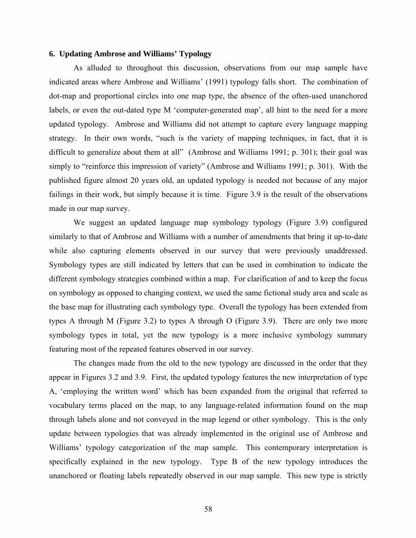
58

6. Updating Ambrose and Williams’ Typology

As alluded to throughout this discussion, observations from our map sample have

indicated areas where Ambrose and Williams’ (1991) typology falls short. The combination of

dot-map and proportional circles into one map type, the absence of the often-used unanchored

labels, or even the out-dated type M ‘computer-generated map’, all hint to the need for a more

updated typology. Ambrose and Williams did not attempt to capture every language mapping

strategy. In their own words, “such is the variety of mapping techniques, in fact, that it is

difficult to generalize about them at all” (Ambrose and Williams 1991; p. 301); their goal was

simply to “reinforce this impression of variety” (Ambrose and Williams 1991; p. 301). With the

published figure almost 20 years old, an updated typology is needed not because of any major

failings in their work, but simply because it is time. Figure 3.9 is the result of the observations

made in our map survey.

We suggest an updated language map symbology typology (Figure 3.9) configured

similarly to that of Ambrose and Williams with a number of amendments that bring it up-to-date

while also capturing elements observed in our survey that were previously unaddressed.

Symbology types are still indicated by letters that can be used in combination to indicate the

different symbology strategies combined within a map. For clarification of and to keep the focus

on symbology as opposed to changing context, we used the same fictional study area and scale as

the base map for illustrating each symbology type. Overall the typology has been extended from

types A through M (Figure 3.2) to types A through O (Figure 3.9). There are only two more

symbology types in total, yet the new typology is a more inclusive symbology summary

featuring most of the repeated features observed in our survey.

The changes made from the old to the new typology are discussed in the order that they

appear in Figures 3.2 and 3.9. First, the updated typology features the new interpretation of type

A, ‘employing the written word’ which has been expanded from the original that referred to

vocabulary terms placed on the map, to any language-related information found on the map

through labels alone and not conveyed in the map legend or other symbology. This is the only

update between typologies that was already implemented in the original use of Ambrose and

Williams’ typology categorization of the map sample. This contemporary interpretation is

specifically explained in the new typology. Type B of the new typology introduces the

unanchored or floating labels repeatedly observed in our map sample. This new type is strictly

59

the result of our study observations; we were unaware of this feature’s use and frequency before

our survey.

Qualitative and quantitative point symbols have been more clearly separated in the new

typology with new symbol type additions to both. Dot-maps and proportional circle symbology

were previously grouped as one type (Type B in Figure 3.2) but are now separated out (Types C

and E respectively in Figure 3.9). Dot maps are separate from the qualitative and quantitative

point symbol types as it was in Ambrose and Williams’ typology because it represents two

possible map variations, one we observed and one we did not. The dot map type observed in our

survey refers to simple points representing the location of, for example, a speaker observation or

language location. We did not observe any quantitative dot density maps, where a dot represents

a certain quantity of feature occurrences within an enumeration unit (Robinson et al. 1995). In

dot density maps, each point does not represent a precise location, rather it represents a set

quantity of the variable that occurs within the unit area. Although we did not observe any dot

density maps in the sample, they are a good possible language visualization to use for conveying

the relative density of language features (Wikle 1997). As a result, we have left the symbology

category of ‘dot maps’ vague so as to include this possible mapping type that may have been (but

did not appear in our sample) or will be used at some point. The new typology features a new

type (type D) of qualitative point symbols, the use of a set of symbols on one map that differ in a

qualitative aspect such as shape or color (but not a color ramp). Qualitative point symbols are

often seen on maps in linguistic atlases that need various ways to symbolize pronunciation

differences. The quantitative point symbol section in Figure 3.9 includes: bar graphs and pie

chart symbols as before; the proportional circles symbology that is now separated from dot-

maps; as well as a new type, type H, of choroplethic or count point symbols. These point

symbols feature a color ramp or numeric value indicating either an ordered degree of a quality

(e.g. status of a threatened language ranging from potentially endangered to extinct) or a count

(e.g. the number of extinct languages). This feature, while only observed in a few maps, was

difficult to categorize using the symbol types in Figure 3.2 and therefore led to the creation of

this new type. Line symbols as a whole remain unchanged between typologies save for the shift

in letters used to represent each type. Diffusion maps are kept in the new typology; they are a

distinct language map type, although they were not included in this survey for reasons discussed

in the methods section.

60

The polygon symbols section received an overhaul in the form of eliminating two types

and renaming a third. Type K in Ambrose and Williams’ typology is removed from the new

version since its distinction isn’t symbology based, but rather map unit-based. The type was

used to indicate maps that used color-shaded political unit polygons for symbolizing language.

This aspect can be accounted for in the new typology by the addition of a superscript to any

polygon-based map type notation. A superscript ‘P’ added to, for example, a map type N (e.g.

NP), would indicate that the polygon map units are politically-based. Type L in Figure 3.2,

choropleth shadings based on a grid, is renamed to ‘Raster’ to represent all grid-based maps.

Finally, the most obvious needed change is the removal of the outdated type M ‘computer

generated map’ from the old typology. Any older SYMAP-type map products encountered can

instead be considered in general as a raster, grid-based map.

Table 3.9 shows the map sample categorized by the new typology. Types M and A were

the frontrunners in frequency of use, matching their counterpart types I and A in Ambrose and

Williams typology (Table 3.7). However, the third most common symbology type, type B

(unanchored/floating labels), is a characteristic that was not captured by the old typology. When

categorized by the updated typology, over 30% of the map sample included a symbology type

(new types B, D, or H) that was not in the Ambrose and Williams’ typology. In other words, a

simple update to the typology, guided by observations made from our map sample, improved the

symbology classification for more than 70 maps in our study sample. The new typology is not

exhaustive as there are always exceptions. However, it does reflect most of the trends that can

be observed on language maps and revitalizes the study of language map construction by

providing a synopsis of language mapping symbology that includes present day practices.

7. Summary and Conclusions

In the absence of guidelines and rules it becomes necessary to learn from actual practices.

In our desire to renew the investigation of language map construction, we studied the symbology

strategies of produced language maps since established language mapping principles are non-

existent. Our survey of language map characteristics supports the generalized typology of

Ambrose and Williams (1991) but also reveals other previously unaddressed trends. We found

many examples of the language mapping problems noted in the literature, such as the prevalence

of solid boundary lines, monolingual mapping, and the use of political mapping units. The

61

survey results provide evidence that these issues cited in the past, with the most relevant

literature at least ten to twenty years old, are still present-day problems. However, we also

observed different attempts to handle these problems, to represent issues of language data

complexity and uncertainty through the use of, for example, unanchored labels, map caveats,

non-solid boundary lines, and overlapping symbology layers. These creative efforts to deal with

language mapping issues indicate that language mapping is not a stagnant cartographic field;

there is room for experimentation with visualization. This is even more so the case given the

technology now available to us, especially with geographic information systems (GIS). The

benefits of GIS, specifically its ease of data organization and the efficient flexibility of

visualization, are important assets not available to language map compilers of the past. With

these new tools at hand, we can review language mapping characteristics as documented in this

research to explore and expand upon the cartographic depiction of language information.

Language will always be an important topic. Tracking the spatial distribution of

language is important for observing, understanding, and appreciating our cultural climate.

Despite their flaws, language maps have consistently been used as textbook figures for lessons

on cultural and linguistic diversity and will remain to serve this function. This survey is an effort

to support and improve upon the educational value of language maps. The survey provides a

summary of what has been done and what has been done the most often. It reveals which tactics

are usual and which ones are rare. It is the starting point for pursuing possible avenues for

improvement and finally fills a void by providing a baseline quantitative account of language

mapping practices, a summary of language mapping methods generated from language maps

themselves. The updated language map symbology typology is a work in progress, created as a

tool intended to be questioned, challenged, and changed as language mapping progresses. Future

research implementing concepts of uncertainty and its representation, exploring the use of raster

surfaces for language data, and collecting volunteered geographic information (VGI) to increase

participation and sample sizes are all potential avenues for language mapping research that can

move the discipline forward (Luebbering In review).

62

8. References

Ambrose, J. E., and C. H. Williams. 1981. Scale as an influence on the geolinguistic analysis of a minority language. Discussion Papers in Geolinguistics 4: 1-16. -----. 1991. Language Made Visible: Representation in Geolinguistics. In Linguistic Minorities, Society and Territory, ed. C. H. Williams, 298-314. Clevedon: Multilingual Matters, Ltd. AustKin. 2009. Map of documented languages. http://austkin.pacific- credo.fr/index.php?page=map (last accessed 3 December 2010). Breton, R. 1991. Geolinguistics: Language dynamics and ethnolinguistic geography. Ottawa: University of Ottawa Press. -----. 1992. 'Easy Geolinguistics' and Cartographers. Discussion Papers in Geolinguistics, 19 – 21: 68-70. Brougham, J. 1986. La periodicite de la geographie linguistique actuelle: essai methodologique (The periodicity of current linguistic geography: a methodological essay). Canadian Geographer 30(3): 206-216. Cohen, S. B. 1973. Oxford World Atlas. New York: Oxford University Press. Comrie, B., S. Matthews, and M. Polinsky, eds. 2003. The Atlas of Languages: The Origin and

Development of Languages throughout the World. New York: Facts on File. Crystal, D. 1997. The Cambridge Encyclopedia of Language. Cambridge: Cambridge University Press. -----. 2005. How language works. London: Penguin Books. Dahlman, C., W. H. Renwick, and E. Bergman. 2010. Introduction to Geography: People, places, and environments. 5th ed. Upper Saddle River, New Jersey: Pearson Prentice Hall. Davis, L. M. 2000. The reliability of dialect boundaries. American Speech 75: 257-259. Dixon, R. M. W. 1972. The Dyirbal language of North Queensland. Cambridge: Cambridge University Press. Dyen, I. 1956. Language distribution and migration theory. Language 32(4): 611-626. Finch, G. 2000. Linguistic terms and concepts. New York: St. Martin's Press. Fouberg, E. H., A. B. Murphy, and H. J. de Blij. 2009. Human Geography: People, Place, and Culture. 9th ed. US: John Wiley & Sons, Inc.

63

Fromkin, V., and R. Rodman. 2002. An Introduction to Language. 6 ed. Orlando: Harcourt Brace College Publishers. Getis, A., J. Getis, and J. D. Fellmann. 2008. Introduction to Geography. 11th ed. New York, NY: McGraw-Hill. Getis, A., J. Getis, M. Bjelland, and J. D. Fellmann. 2010. Introduction to Geography. 13th ed. New York, NY: McGraw-Hill. Greenberg, J. H. 1987. Language in the Americas. Stanford, CA: Stanford University Press. Gregory, D., R. Johnston, G. Pratt, M. Watts, and S. Whatmore, eds. 2009. The Dictionary of

Human Geography. 5th ed. Malden, MA: Wiley-Blackwell. Hall, R. A., Jr. 1949. The linguistic position of Franco-Provencal. Language 25: 1 - 14. Harmon D. 1996. Losing species, losing languages: Connections between biological and linguistic diversity. Southwest Journal of Linguistics 15: 89–108. Hoch, S., and J. J. Hayes. 2010. Geolinguistics: The incorporation of geographic information

systems and science. The Geographical Bulletin 51: 23-36. Horton, D. R. 2009. Indigenous Language Map. http://www.abc.net.au/indigenous/map/ (last

accessed 3 December 2010). Kahane, H. R. 1941. The project of the Mediterranean linguistic atlas. Italica 18: 33-36. Kessler, F., and T. Slocum. 2011. Analysis of Thematic Maps Published in Two Geographical

Journals in the Twentieth Century. Annals of the Association of American Geographers 101(2): In press.

Kirk, J. M., S. Sanderson, and J. D. A. Widdowson. 1985. Introduction: Principles and practice

in linguistic geography. In Studies in linguistic geography: The dialects of English in Britain and Ireland, eds. J. M. Kirk, S. Sanderson and J. D. A. Widdowson, 1–33. London: Croom Helm.

Knox, P. L., and S. A. Marston. 2010. Human Geography: Place and Regions in Global

Context, 5th ed. Upper Saddle River, New Jersey: Pearson Prentice Hall. Kretzschmar, W. A., Jr. 1997. Generating linguistic feature maps with statistics. In Language variety in the South revisited, eds. C. Bernstein, T. Nunnally, and R. Sabino, 392-416. Tuscaloosa: University of Alabama Press. Kurath, H. 1931. The geography of speech: Plans for a linguistic atlas of the United States and

Canada. Geographical Review 21: 483-486.

64

Lameli, A. 2010. Linguistic atlases – traditional and modern. In Language and Space: An international handbook of linguistic variation. Volume 1: Theories and methods, eds. P. Auer and J. E. Schmidt, 567-592. New York: De Gruyter Mouton.

Lee, J., and J. W. A. Kretzschmar. 1993. Spatial analysis of linguistic data with GIS functions.

International Journal of Geographical Information Systems 7: 541-560. LL-Map. 2009. Language and Location: A map annotation project. http://llmap.org/ (last accessed 3 December 2010) Luebbering, C. R. In review. Displaying the geography of language: the cartography of language maps. Submitted to The Cartographic Journal. Macaulay, R. K. S. 1985. Linguistic maps: Visual aid or abstract art? In Studies in linguistic

geography: The dialects of English in Britain and Ireland, eds. J. M. Kirk, S. Sanderson, and J. D. A. Widdowson, 172–186. London: Croom Helm.

Mackey, W. F. 1988. Geolinguistics: Its scope and principles. In Language in geographic

context, ed. C. H. Williams, 20-46. Philadelphia: Multilingual Matters, Ltd. Maffi, L. 2005. Linguistic, Cultural, and Biological Diversity. Annual Review of Anthropology

29: 599-617. Marston, S. A., P. L. Knox, D. M. Liverman, V. Del Casino, and P. Robbins 2010. World Regions in Global Context: Peoples, Place and Environments. 4th ed. Upper Saddle River, NJ: Pearson Prentice Hall. Masica, C. P. 1976. Defining a Linguistic Area: South Asia. Chicago: University of Chicago

Press. McDavid, R. I., Jr.,, V. G. McDavid, W. A. Kretzschmar Jr., T. K. Lerud, and M. Ratliff. 1986.

Inside a linguistic atlas. Proceedings of the American Philosophical Society 130: 390-405.

Menner, R. J. 1933. Linguistic geography and the American atlas. American Speech 8: 3-7. Milner-Gulland, R., and N. Dejevsky. 1998. Cultural Atlas of Russia and the Former Soviety Union. New York: Checkmark Books. Norton, W. 2010. Human Geography. 7th ed. Canada: Oxford University Press. O'Cain, R. K. 1979. Linguistic atlas of New England. American Speech 54: 243-278. Ormeling, F. 1992. Methods and possibilities for mapping by onomasticians. Discussion Papers

in Geolinguistics 19-21: 50-67.

65

Pederson, L. 1993. An approach to linguistic geography. In American Dialect Research, ed. D. R. Preston, 31-92. Philadelphia: John Benjamins Publishing Company.

Peeters, Y. J. D. 1992. The political importance of the visualisation of language contact.

Discussion Papers in Geolinguistics 19-21: 6-8. Powell, J. W. 1891. Linguistic Stocks of American Indians North of Mexico. In Seventh Annual

Report of the Bureau of Ethnology to the Secretary of the Smithsonian Institution, 1885-’86.

Robinson, A. H., J. L. Morrison, P. C. Muehrcke, A. J. Kimerling, and S. C. Guptill. 1995.

Elements of Cartography. 6th ed. United States: John Wiley & Sons, Inc. Rubenstein, J. M. 2008. The Cultural Landscape: An Introduction to Human Geography. 9th ed. Upper Saddle River, NJ: Pearson Prentice Hall. -----. 2010. The Cultural Landscape: An Introduction to Human Geography. 10th ed. Upper Saddle River, NJ: Pearson Prentice Hall. SIL International. 2007. Languages of Nigeria. Digital file received from R. Blench. Shibatani, M. 1990. The Languages of Japan. New York: Cambridge University Press. United States Central Intelligence Agency. 1997. Ethnolinguistic groups in Afghanistan. Map No. 802551. http://www.lib.utexas.edu/maps/middle_east_and_asia/afghanistan_ethnoling_97.jpg (last accessed 3 December 2010) United States Central Intelligence Agency. 1979. Linguistic Groups. Map No. 504014. http://www.lib.utexas.edu/maps/africa/nigeria_linguistic_1979.jpg (last accessed 3 December 2010) Wagner, P. L. 1958. Remarks on the geography of language. Geographical Review 48: 86-97. Wikle, T. 1997. Quantitative mapping techniques for displaying language variation and change.

In Language variety in the South revisited, eds. C. Bernstein, T. Nunnally, and R. Sabino, 417-433. Tuscaloosa: University of Alabama Press.

Wikle, T., and G. Bailey. 2010. Mapping North American English. In Language and Space: An international handbook of linguistic variation. Volume 2: Handbook to Linguistic Mapping, eds. A. Lameli, R. Kehrein, and S. Rabanus, 253-268. New York: De Gruyter Mouton. Williams, C. H. 1996. Geography and contact linguistics. In Contact linguistics: An

International Handbook of Contemporary Research, eds. H. Goebl, P. H. Nelde, Z. Stary, and W. Wolck, 63-75. New York: Walter de Gruyter.

66

Williams, C. H., and J. E. Ambrose. 1988. On measuring language border areas. In Language in

geographic context, ed. C. H. Williams, 93-135. Philadelphia: Multilingual Matters, Ltd. -----. 1992. Geolinguistic Developments and Cartographic Problems. Discussion Papers in

Geolinguistics 19-21: 11-32. Williams, C. H., and I. Van der Merwe. 1996. Mapping the multilingual city: A research agenda

for urban geolinguistics. Journal of Multilingual and Multicultural Development 17: 49-66.

Woodard, R. D., ed. 2004. The Cambridge Encyclopedia of the World’s Ancient Languages.

Cambridge: Cambridge University Press. Wurm, S. A., and S. Hattori, eds. 1981. Language atlas of the Pacific Area. Canberra: The Australian Academy of the Humanities in collaboration with the Japan Academy.

67

 

  Figure 3.1. World language map figure in a textbook for introductory human geography. Close inspection of this map reveals conflicting messages about the map’s information. The legend is titled “indigenous languages” while the caption reads “major language and major language families”. Three different sources were used for map compilation with no discussion of their respective methodologies. (Image source: Knox and Marston 2010)

68

 Figure 3.2. Ambrose and Williams (1991) diagram showing common language mapping symbols.

69

  

  

 Figure 3.3. Distribution of source types for the map sample.

17%

24%

9%13%

4%1%

3%

4%

25%Atlas

Book

Government Publication

Journal Article

Map Product

Newspaper

Organization

Textbook

Website

70

  

    

Figure 3.4. Distribution of publication decades for maps and map sources (7 websites without dates excluded).

0

10

20

30

40

50

60

70

80

90

100

Count

Years

Sources

Maps

71

 

 Figure 3.5. Use of non-solid line boundaries for visual distinction, not to indicate uncertainty or fluidity of data (Image source: Shibatani 1990).

72

  

Figure 3.6. Map symbology strategies observed for visualizing multilingualism.  

73

  Figure 3.7. Unique examples of language map uncertainty and boundary depiction: a) use of crisp and undefined boundaries (Image source: Powell 1891); b) question marks (Image source: Wurm and Hattori 1981); c) zipper-like boundary for language intermingling (Image source: Cohen 1973); and d) map category for unknown areas (Image source: Greenberg 1987).  

74

  Figure 3.8. Examples of unanchored or floating language labels. Image sources: a) Woodard 2004; b) Getis, Getis, and Feldmann 2008; c) Dixon 1972.

75

 Figure 3.9. Updated Ambrose and Williams’ (1991) typology of language mapping symbology types based on map survey observations.

76

 Table 3.1. Frequency of coverage extents used in the map sample.

                   Table 3.2. Use of points, lines, and polygons for language data depiction. Note: Percentages sum to greater than 100% since some maps used more than one symbol dimension.  

Symbol Dimension Used # of maps % of maps Points 61 25.42 Lines 46 19.17

Polygons 162 67.50  

 

Map Coverage Extent # of maps % of map sample World 29 12.08 Continent(s) 34 14.17 Region (extends beyond one country) 36 15.00 Country 91 37.92 Region within a country 35 14.58 US State 3 1.25 City or Community 12 5.00 TOTAL 240 100.00

77

Table 3.3. Generalized language variable types and frequency of use within the map sample.  Generalized Language Map Variables Includes: # of maps % of maps Counts or Proportions Counts or proportions of speakers, counts or proportions of languages 26 10.83

Ethnolinguistic or linguistic groups 11 4.58

Languages 89 37.08

Language features Accents, creoles, dialects, dialect divisions, linguistic features, pidgins, pronunciation, vocabulary, word usage 78 32.50

Language importance or use Dominant languages, English status or use, leading languages, major languages, minor languages, mother tongue, official languages 20 8.33

Language relationships or categorization Language branches, language families, language groups, language homeland, language origin, language phyla, language stock, language subfamilies, language subgroups, language subphylum

64 26.67

Language status (ex. extinct, threatened) Documented languages, language hotspots, number of threatened languages, phases of language decline, threatened status of language 9 3.75

Other Bilingualism rate/bilingualism divide; measurements: language diversity, versatility, diversity index, frequency scores, functional importance; speech area; temporal extent of speaking area

13 5.42

 

78

Table 3.4. Use of solid versus non-solid boundary lines for language items on maps. Note: Percentages do not sum to 100%; three maps were double-counted as ‘Yes’ and ‘No’ because some language features on the map used line symbology while others did not.  Used solid boundary lines for language items? # of maps % of map sample

% of maps with language item boundary lines

Yes 112 46.7% 57.1% No 84 35.0% 42.9% N/A 47 19.6%

      Table 3.5. Most common map unit categories and use of political map units observed in the sample. Note: Many maps use more than one unit type for language data and are therefore counted for each unit type used.  

              

            

Map Unit Category # of maps % of map sample Language area (polygon) 77 32.08 Language family area (polygon) 38 15.83 Observation location (point) 25 10.42 Language location (point) 23 9.58 Isoglosses (line) 18 7.50 Dialect area (polygon) 17 7.08 Country (polygon) 14 5.83 Political Map Unit 43 17.80 Non-Political Map Unit 198 82.20

79

Table 3.6. Number of language items and language items per place observed in the map sample.  Number of different languages or language features on the map # of maps % of map sample

1 43 17.9 >1 197 82.1

Number of language items per place # of maps % of map sample % of applicable maps

1 117 48.8 59.4 >1 80 33.3 40.6

     Table 3.7. Use of Ambrose & Williams’ symbology types and the top symbology types overall (combinations included). Refer to Figure 2 for the definition of each symbology type.  Type # of maps % of maps Top Types # of maps % of maps

A 89 37.08 I 49 20.42 B 51 21.25 AI 41 17.08 C 1 0.42 B 25 10.42 D 2 0.83 A 23 9.58 E 33 13.75 Sum 138 57.50 F 8 3.33 G 1 0.42 I 112 46.67 J 22 9.17 K 32 13.33 L 4 1.67

             

80

Table 3.8. Sample of map caveat quotes observed. “Location of languages is approximate.” (AustKin 2009) “Boundary representation is not necessarily authoritative.” (United States Central Intelligence Agency 1997) “The boundaries on this map are somewhat artificial and pockets of speakers of other languages will be found in areas where one language is dominant.” (Comrie, Matthews, and Polinsky 2003, p. 141) “By suggesting that the area assigned to a language or language family uses that language exclusively, the map pattern conceals important linguistic detail. Many countries and regions have local languages spoken in territories too small to be recorded at this scale.” (Getis, Getis, and Feldmann 2008, Figure 7.19, pp. 236-7) “This map indicates only the general location of larger groupings of people which may include smaller groups such as clans, dialects or individual languages in a group. Boundaries are not intended to be exact.” (Horton 2009) “Well over 100 languages are spoken in the region, the majority of them by very small ethnic groups, and hence unrecordable on any save the most detailed maps.” (Milner-Gulland and Dejevsky, 1998, p.26) “Although the country can be divided into four main linguistic regions as shown, people living in individual communities, especially in the mountains, may use a language other than the prevailing local one.” (Rubenstein, 2008, p.171)

81

Table 3.9: Use of new typology symbology types and the top symbology types overall (combinations included). Refer to Figure 9 for the definition of each symbology type.  Type # of maps % of maps   Top Types # of maps % of maps

A 89 37.08   M 58 24.17 B 39 16.25   AM 27 11.25 C 15 6.25   N 21 8.75 D 32 13.33   ABM 15 6.25 E 3 1.25   A 13 5.42 F 1 0.42   D 13 5.42 G 2 0.83    H 4 1.67    I 33 13.75    J 8 3.33    K 1 0.42    M 128 53.33    N 22 9.17    O 4 1.67    

 

82

Chapter 4: Visualizing Linguistic Diversity through Cartography and GIS: A case study

of commonly used techniques and the potential of linguistic diversity index mapping

Abstract:

Language maps are used as educational tools in textbooks, on websites, and in magazines

and newspapers. Providing a snapshot of the spatial distribution of languages and cultures,

language maps are valuable visual aids that can accompany and improve discussions of our

current cultural climate. With language somewhat intangible, it is a difficult variable to map and

yet there are no established guidelines for cartographers who take on this challenge. While there

are many design hurdles with language maps, it is the perception of power conveyed by such

maps that is perhaps the most meaningful issue. Whether through design constraints or

deliberate choice, many language maps show only one language per place (monolingual

mapping). In reality, many places in our current world are misrepresented by this linguistically

one-dimensional mapping approach. This research explores the cartographic visualization of

linguistic diversity. Using the Washington, D.C. metropolitan statistical area and publicly

available language data from the 2000 census, we first create and critique symbology methods

modeled after language maps in use. Next, we explore the application of a linguistic diversity

index as a mapping variable for both vector and raster environments and the potential of the

resulting maps to serve as new figures for lessons on linguistic diversity in educational contexts.

Key Words: cartography, diversity index, GIS, language, linguistic diversity

1. Introduction

Delving into language facts produces some astounding numbers: there are approximately

6,900 living languages in the world today; 364 of these are used as first languages by residents of

the US (Lewis 2009). These numbers are interesting, but their immediate implications are

unclear. It is important to revisit the reason language is included in our geography curricula and

why we bother mapping it. As Trueba (1993) states:

“Culture and language are so intricately intertwined that even trained scholars find it

impossible to decide where language ends and culture begins, or which one of the two

impacts the other the most” (p. 26).

83

Language is an intricate part of culture and therefore a necessary component to understanding

our cultural climate. With language as a lens for viewing culture, language maps provide insight

to the movements and distributions of culture. The belief of this notion is evidenced by the

prolific use of language maps in introductory geography textbooks (e.g. Fouberg, Murphy, and

de Blij 2009; Dahlman, Renwick, and Bergman 2010; Getis et al. 2010; Knox and Marston

2010; Marston et al. 2010; Rubenstein 2010).

Serving as important visual aids for lessons on cultural and linguistic diversity, textbook

maps should make use of current mapping technology to convey the world’s linguistic diversity

to our students, yet they do not seem to do so. Past research is not kind in describing the typical

world language maps of textbooks and atlases or even language maps in general. They are

labeled boring (Williams and Ambrose 1992), outdated (Brougham 1986), oversimplified

(Mackey 1988), and lacking in creativity (Williams 1996). Often language maps remain

relatively unchanged through subsequent textbook editions despite the constant linguistic change

occurring in the world. However, there may be a reason for the stagnation of language mapping

design progress. The translation of an intangible social and cultural variable such as language to

a map product is a challenging task. Forcing language into the typical realm of points, lines, and

polygons is unnatural and requires endless compromises between reality and representation.

Among many issues, language maps often encounter the problem of power and perception.

When maps are unable, due to symbology or scale limitations, to represent all languages in a

locale, subsets of languages (or even just one language) are chosen for representation over

others. The language speakers passed over for representation are disempowered and their

presence left undocumented for map users. These design issues directly conflict with the idea of

mapping linguistic diversity and may explain the hesitation to explore linguistic diversity

mapping possibilities. Fortunately, we have new tools at our disposal to try to push language

mapping forward. Geographic information systems (GIS) are presently underutilized for spatial

analysis and display of language data (Hoch and Hayes 2010), but offer flexibility in data

storage, analysis, and display unrivaled by previous mapping software.

The rapid change of the linguistic composition of the United States directs our focus on

mapping linguistic diversity among other possible language variables. Although often viewed as

a monolingual block of English, the United States has housed the most immigrant languages of

84

any developed nation and has a history of linguistic diversity stemming from the country’s

colonial days (Heath 1981; Wiley 1996; Bayley 2004). Less than half of the 300 plus living

languages in the United States are indigenous to North America; 52% are immigrant languages

(Lewis 2009). Based on estimates from the 2007 American Community Survey, 20% of the US

population speaks a language other than English in their homes (Shin and Kominski 2010).

From 1980 to 2007, the United States population increased by 34%; the percentage of speakers

of languages other than English grew 140% (Shin and Kominski 2010). These changes in the

linguistic composition of the United States have been accompanied by fierce debate as well as

educational and governmental policies regarding language. Some movements embrace the

growth of diversity; others rally behind English-only pursuits. The constant shifting of feelings

towards non-English speakers is said to represent the United States’ ambivalent view of

linguistic diversity (Nieto and Bode 2008). In the context of a society that is inarguably

increasing in linguistic diversity, the nation-wide implications of language-related policy need to

be considered (Nieto and Bode 2008). The contentious issue of language in a country

undergoing rapid changes in its linguistic composition makes the task of producing language

maps of the U.S. a highly valuable endeavor.

This visualization study explores alternatives to monolingual mapping (one language per

place) to convey the linguistic diversity of an area. Using the Washington, D.C. metro area as

our case study site, we critique the ability of different mapping strategies to convey the presence

of linguistic diversity to map viewers. While some mapping strategies are modeled after current

language map products, we also investigate the use of an established linguistic statistic, the

linguistic diversity index, as a map variable. Following the language surface work of Wikle

(1997) and Taylor (1977), we attempt to create a ‘linguistic diversity surface’ as a new mapping

alternative for overcoming the commonly cited problems of mapping language in a discrete,

vector environment. Our work addresses two main research questions: 1) can today’s mapping

technology produce meaningful representations of linguistic diversity (rather than language

dominance) to serve as educational or research tools, and 2) are there other measures available,

such as the linguistic diversity index, that could serve as useful language mapping variables?

Language maps have been consistently utilized for educational purposes while their construction

and design implications concerning the representation of linguistic diversity have been left

relatively unchallenged and unexplored using today’s technology. As the linguistic diversity of

85

societies (like the U.S.) increases, language maps that can reflect these trends and represent the

linguistic community as a whole will be helpful for understanding the cultural and societal

change we see and hear around us.

2. Related Work

2.1. Difficulties and Limitations of Current Language Mapping Practices

Although language maps appeared as early as the 1700s (Lameli 2010), there has yet to

be actual established guidelines for language map construction (Kirk, Sanderson, and

Widdowson 1985; Ambrose and Williams, 1991; Williams, 1996). Ambrose and Williams

(1991) and Ormeling (1992) summarize language map symbology types, but the recent work of

Luebbering, Kolivras, and Prisley (In prep) is the first to systematically survey the cartographic

characteristics of produced language maps to deduce common practices of language map

construction as a starting point for documenting language mapping in practice and developing

general guidelines. Language mapping is a difficult task that could benefit from some guidance.

Language is a continuous and fluctuating cultural phenomena with one language blending into

another (Breton 1991). These are not characteristics of a variable that readily translate to map

composition. At best, a language map represents a linguistic snapshot in time. Speaker

distributions before or after that moment, or that dataset, are undoubtedly different. Further,

language is often viewed as an important component to one’s identity. A person identifies with

their language on a map or feels unidentified if their language is not visible. Considering this, it

is clear that all map viewers will never agree upon one authoritative language map (Peeters

1992).

Many language map issues stem from the practice of using a discrete vector environment

for portraying language data. One prominent problem is map unit selection. From the onset of

map compilation, the available options for language map units are always second best. The ideal

mapping unit would be the single unit at which a given variable occurs. In the case of language,

that ideal mapping unit is an individual speaker, a unit that is typically off limits due to important

considerations of anonymity and confidentiality. As a result, language data is frequently

aggregated into or collected on the basis of areal units. This areal aggregation is problematic

given its inconsistency with the level at which language actually occurs (Williams 1996).

Compounding this problem is the tendency to use political mapping units for language maps (ex.

86

counties or states) (Williams 1996). Such mapping units can change over time, have irregular

boundaries, and be based on random decisions (Ambrose & Williams 1991). Macaulay (1985)

notes how counties are sometimes used in linguistic atlases despite no evidence validating their

relationship to dialect boundaries. Both Ormeling (1992) and Williams (1996) point out the

inaccurate portrayal of language as completely homogenous within administrative boundaries

when administrative units act as language map units.

Boundary depiction is another vector-related problem in language mapping. While

problematic in many mapping tasks, boundary depiction faces unique challenges in the case of

language data. Language boundaries sometimes result from arbitrary choices (Macauley 1985).

An individual researcher may produce a language boundary solely based on their personal

interpretation of observation data points (Kirk, Sanderson, and Widdowson 1985; Ormeling

1992). This practice produces the possibility of different boundaries generated from the same

dataset at the hands of different researchers (Ormeling 1992). The dataset itself also contributes

to boundary variation; the choice of what to collect can alter resulting dialect or language

boundaries (Mackey 1988; Williams and Ambrose 1988; Davis 2000). Reflecting the absence of

general language mapping guidelines, there is no commonly held convention as to what

characteristic a language boundary should represent (Williams and Ambrose 1988). Each

approach to boundary definition and depiction can create a different spatial rendition of a

language environment so all language boundaries should be interpreted with caution. The issue

of language boundaries even reaches the issue of lines themselves and whether such a discrete

one-dimensional symbology is appropriate for language depiction. Lines portray

authoritativeness beyond that which language maps can usually claim (Williams 1996) and are

ill-suited to reflect the complexity of processes that take place along modern-day language

boundaries (Williams and Ambrose 1988). Areas, zones, or belts are the terms used by

researchers to describe language boundaries (Hall Jr. 1949; Masica 1976; Kirk, Sanderson, and

Widdowson 1985; Breton 1991; Ormeling 1992). Covering large areas and encapsulating

complicated social and linguistic structures (Kirk, Sanderson, and Widdowson 1985; Breton

1991), the characteristics of language transition areas or ‘linguatones’ (Luebbering In review) are

oversimplified and unacknowledged when represented by lines.

87

2.2. Power and Perception in Language Mapping

In our effort to visualize the spatial distribution of linguistic diversity, we are tackling a

major joint issue of language mapping in a vector format: power and perception. Language

maps often display the strategy of attaching only one language to a location. Luebbering,

Kolivras, and Prisley (In prep) found that among maps showing the distribution of more than one

language feature or language, 59% displayed only one per place. This tendency of monolingual

mapping is unsuitable for many places in the world known to be linguistically diverse.

Implementation of monolingual mapping for most study areas involves a choice of whose

language to symbolize and whose language(s) are left off the map. Breton (1992) explains how

map symbology limitations expose the power struggles among different languages.

Cartographers must often take sides, choose who they will represent on the map, and as a result

hide an area’s linguistic diversity. For example, the simplified world language maps of

textbooks and atlases most often feature state languages, exaggerating their spatial extent while

marginalizing the presence of all non-official languages (Williams and Ambrose 1992). The

placement of language boundaries is also a sensitive matter that can instigate heated debate and

influence who benefits from political policy initiatives (Williams and Ambrose 1992; Williams

1996). Navigating the relationships of dominant and minority languages, and the accompanying

symbology compromises, sometimes produces a mapping outcome that can misinform map

viewers. Our research embraces this aspect of power and perception in language mapping and

aims to creatively overcome such limitations to produce useful maps that feature linguistic

diversity, not linguistic majority.

2.3. Quality of Census Data on Language

Language data collected in national censuses are frequently used for language mapping as

is the case for this study as well. Census language data are accessible, provide thorough spatial

coverage, and offer a great cost savings for data gathering. Many countries have collected

language data over a long period of time that researchers can use to ascertain linguistic

conditions of the past (Lieberson 1981). Also, using census language data provides a broader

context to studies, allowing the comparison of local findings with trends in other parts of the

country (Lieberson 1981). Overall, the census is the best tool for gauging language diffusion

(Breton 1991) and an important source for geolinguistic analysis in general (Williams 1984).

88

Despite these advantages, census data on language must be used with caution given a number of

issues including question type, question wording, question ambiguity, and interpretation limits.

Users of census data must also remember that the census (in many instances) is a widely

distributed self-administered questionnaire (Williams 1988), leaving it subject to unintentional

errors from misinterpretation (Lieberson 1981) and the biases inherent in self-reporting

(Williams 1984). Language question utility depends on both the intention of the question and the

actual interpretation of it (Mackey 1988). Any ambiguity in questions leaves respondents unsure

of what their appropriate response should be. For example, truly bi- or multilingual individuals

may struggle with questions about the language they first learned (Lieberson 1981). Questions

about language ability in particular are complicated for both those providing and those using

responses since there is no clear definition of what skills equate with the listed ability levels

individuals must choose from (Lieberson 1981).

A final major criticism of census-collected language data is that it is too simplistic in its

queries. Ambrose (1980) criticizes that most censuses fail to capture real indicators of the actual

practice of language use and therefore, as echoed by Williams (1984), fall short in helping to

understand language change. Respondents are not asked about speech domains, speech styles, or

spoken language frequency; queries focus only on whether or not they speak given languages

(Williams 1984). In light of these acknowledged shortcomings, researchers note how census

language data must be scrutinized and used cautiously (Lieberson 1981; Breton 1991).

2.4. Language Map Production and Analysis with GIS

A number of recent works are renewing attention to the issue of language mapping.

Hoch and Hayes (2010), Luebbering (In review), and Wikle and Bailey (2010) all provide

different literature review perspectives on the topic of the spatial display and analysis of

language data. While all of these works emphasize the potential of GIS and contemporary

analysis tools, they do not undertake detailed case studies of their application. Researchers laud

the potential of GIS for linguistic data (Williams and Ambrose 1992; Lee and Kretzschmar 1993;

Williams 1996; Williams and Van der Merwe 1996; Kretzschmar 1997) however geolinguistic

research has thus far made little use of GIS (Hoch and Hayes 2010). There is discussion of

spatial analysis possibilities (Lee and Kretzschmar 1993) including spatial autocorrelation and

density estimation (Kretzschmar 1997) but more recent research is rather absent. Besides our

89

previous study surveying language map characteristics (Luebbering, Kolivras, and Prisley In

prep), only Wikle (1997) has specifically addressed and explored mapping techniques for

language data. Wikle’s (1997) exploration of the quantitative mapping of language data

provides the framework for our own investigation. Wikle (1997) uses linguistic survey data (ex.

vocabulary usage and pronunciation) and early mapping software (Atlas Graphics and

MapViewer) to explore areal, point, and surface mapping to detect language variation and

change. Over ten years after his work, we use publically available language data and

contemporary GIS software to explore areal, point, and surface visualizations of linguistic

diversity, including the application of an established statistic as a new mapping variable. To

reinvigorate the topic of language mapping, we explore the socially relevant issue of linguistic

diversity by creating maps for educational or research contexts that feature rather than mask this

cultural characteristic.

3. Language and Base Map Data

3.1. Language Dataset

The language dataset used for map compilation in this visualization study comes from the

2000 US Census and is available online from the Census Bureau’s website (www.census.gov).

The data are compiled from the census question asking respondents what language they speak at

home. In terms of language question types, this is a question of language use by Mackey’s

(1988) definition; for Lieberson (1981) it is a question of the language most commonly used at

home when the census data were collected. This question appeared on the long form of the 2000

Census that was supplied to approximately one out of every six households (US Census Bureau

2007). The census tract level data are compiled in Special Tabulation 224, Detailed Language

Spoken at Home for Population 5 years and over, released in April 2004 (US Census Bureau

2004). The special tabulation lists 71 languages or language categories for our study area. This

is considerably more detailed language data than the Census Bureau usually supplies. The

Census Bureau most often uses either four major language groups or 39 detailed language groups

of aggregated language information (US Census Bureau 2010). As revealed by the discussion in

the literature review, census language data are problematic. Any patterns or analyses computed

from census language data must be interpreted cautiously. For example, the census collects data

on where people live, not where they work. In our dataset of Washington, D.C., the census tracts

90

covering the National Mall area have no language data since no one lives on the Mall, however,

many people work there. Despite issues with the census, it is still one of the best resources

available for widespread language data and the most suitable for our visualization study given its

accessibility and even geographic coverage. In this respect, we use the census language dataset

as a means of showing language mapping possibilities for any suitable language dataset, not just

information from the census.

3.2. Study Area and Base Map Files

In order to best explore the utility of different map types for showing linguistic diversity,

we need to focus on a study area that is likely to be linguistically diverse. Given that large cities

tend to have greater linguistic diversity than less populated areas, combined with the authors’

familiarity and proximity, we chose Washington, D. C. to serve as the study area. In order to

include the greater Washington, D. C. area and to match the source of our language dataset (the

US Census), we use the Washington-Arlington-Alexandria, DC-VA-MD-WV Metropolitan

Statistical Area (D.C. MSA) as defined by the United States Census Bureau. The D.C. MSA

includes the District of Columbia, 15 Virginia counties, 5 Maryland counties, and 1 West

Virginia county (Office of Management and Budget 2008; Figure 4.1). The study area is

composed of 1016 census tracts (5 do not have language data available and will be noted as ‘No

Data’ in all figures), the largest scale of map unit at which the data are available. Since the

language dataset comes from the US Census and is organized according to census geography, we

used US Census TIGER files for the base map. TIGER files are available both from the US

Census Bureau’s website (www.census.gov) as well as through ESRI online

(http://arcdata.esri.com/data/tiger2000/tiger_download.cfm). Base map layers include all census

tracts and counties in the D.C. MSA.

4. Case Study of Visualization of Linguistic Diversity

With our own and others’ previous research indicating the tendency for linguistic

diversity to be masked in language maps, we undertake a case study for visualizing linguistic

diversity for the D.C. MSA using the census language dataset in a GIS (ArcGIS 9.3 software).

We begin by recreating with our dataset the themes and map types observed in other language

maps. For each map, we discuss the methods of construction as well as the advantages and

91

disadvantages concerning the ability to convey the quality of linguistic diversity for the study

area. [Note: English is referred to as the majority language in the US, having the most speakers

in the country as a whole, while all other languages are referred to as minority languages even

though speakers of minority languages outnumber English speakers in some places.]

4.1. Leading Languages after English

Farley and Listar (2007) aim to capture the linguistic and ethnic diversity of Toronto by

mapping, using census tracts, the leading language after English in terms of speaker population.

The result is a ‘language quilt’ (the title of their work) revealed by peeling back the dominating

cover of English (Farley and Listar 2007). Figure 4.2 is modeled after their map using the D.C.

MSA dataset. As non-linguists constructing a language map, we want to ensure that our

symbology does not indicate any qualities of language other than visually distinguishing one

language from the other. Fill colors are carefully assigned to not create any pattern or color

gradation that could imply language relatedness. There was not always a clear second language

after English. In some census tracts (8 tracts) two languages are equally prominent or there is

even three-way tie (1 tract). For these tracts we use a two or three stripe fill with stripes of equal

width, one of each color for the respective languages, angled at 45 degrees. There were also

tracts where English was not the language with the most speakers (15 tracts). For these instances

we used the backdrop color of the leading language, with a thin horizontal line pattern (in the

dark blue color representing English) overtop with considerable separation between lines (see

large scale inset map, Figure 4.2). Farley and Listar (2007) did not note this quality through their

symbology, rather they created a separate section on their map entitled “Where English is the

second language…and even the third” with inset maps of such neighborhoods.

This map is an interesting departure from typical language maps encountered;

Luebbering, Kolivras, and Prisley (In prep) encountered only two out of 240 language maps in

their survey that mapped second leading languages. It visually removes the common knowledge

that English is predominantly spoken in the United States to reveal the less explored topic of

minority languages. The map, which exposes the viewer to the presence of linguistic diversity,

has the potential to reveal ethnic enclaves, though not as well as other data and symbology

strategies. More importantly, the map can serve as a foundation for beginning to explore

linguistic diversity. It isn’t quantified (we don’t show speaker percentages) and it isn’t holistic

92

(we don’t show all the languages present in each tract), but it acknowledges the presence, after

English, of at least 14 other language categories to map viewers.

Concerning the shortcomings of this map, are we simply substituting one dominating

blanket of language for another? In a country like the US that has one dominating minority

language [Spanish has 34.5 million speakers, almost fourteen times as large as Chinese, the next

nearest language (Shin and Kominski 2010)], are all other minority languages masked in this

map due to the dominance of the largest minority language? Spanish is the leading language

after English in 879 census tracts, or 87% of the study area tracts. It visually appears to

dominate the map perhaps indicative of its ‘blanket’ status. However, Spanish’s visual

dominance may be deceiving. This deception illustrates a major issue with this mapping

strategy for showing linguistic diversity. The language chosen for representation for a census

tract simply has to have more speakers than the next language. It did not have to have a certain

magnitude more, just one more speaker. Spanish may represent a census tract where it has only

10 more speakers than the next language; in other words, the language that is used to symbolize

the census tract may have won by the slimmest of margins. Of course this may also mean that

English could be the majority language in census tracts by the slimmest of margins as well; there

may be more census tracts where the idea of the ‘leading language after English’ is less

applicable since such languages come close to tying the English population. Accounting for the

sampling error in the dataset would cause further issues. Some tracts would be in question as to

which language is the true leading language if multiple language populations fall within the

sampling error margin.

4.2. Percentage of Individual Language Speakers

The Modern Language Association’s Language Map (Modern Language Association

2010) uses US Census 2000 data to provide an online interactive mapping tool for students,

educators, and web surfers alike for exploring the distribution of languages in the United States.

Users select a state to view (or view the continental US), a language, and how they would like to

view the language data (either percent by county, number by county, or number by zip code)

resulting in a choropleth map based on their choices. Using the D.C. MSA language dataset,

Figure 4.3 is modeled after the MLA language map, specifically using the percentage of Spanish

speakers by census tract. We used seven classes for the map; six classes established using

93

natural breaks (as advocated by Wikle 1997) with a separate category for tracts with 0%. This is

modeled after the six classes used in the MLA map with the additional improvement of the

separate category for 0% to visually distinguish tracts with no Spanish speakers (Note: the

language data is based on a sample of households; there may be Spanish speakers in these tracts

that were not captured).

Following our discussion of Figure 4.2, we can sort out the extent of Spanish’s

dominance as the largest minority language using Figure 4.3 since it shows the actual percentage

of residents who speak Spanish in their homes. In this respect this type of map solves one of the

problems of the leading language map; it quantifies language. We can see not just a language’s

presence, but how many resident speakers there are. Our map is a slight improvement of the

MLA map in terms of the scale of both map units and data categories. The largest scale map

units for the MLA map are limited to county or zip code, while we have detailed language

information down to the census tract. Further, as stated in describing the dataset, we have a

detailed list of 71 languages or language categories noted as present in the D.C. MSA by the

census; the MLA map only features a summarized list of 33 languages or language groups other

than English.

The primary disadvantage of this map, and any modeled after it, is the limited coverage

of its subject matter. Figure 4.3 does quantify language, however it only quantifies one language

at a time. To see all of the languages present in the study area and their relative quantities would

require a series of maps. The MLA map allows users to show up to two maps at once for

comparison, but this still falls short of providing viewers a fast and comprehensive view of

linguistic diversity in the region.

4.3. Percentage of Speakers of all Non-majority Languages

With the mapping strategies described above, we have thus far been unable to both

quantify language speakers as well as represent all minority languages within one map. A

different approach that may achieve this end is another data display option offered by the MLA

map (Modern Language Association 2010) and used by the US Census in one of its language

map products (U.S. Census Bureau 2000): mapping the percentage of speakers of all non-major

languages, or in our case, speakers of all languages other than English. Figure 4.4 follows these

examples by mapping the percentage of residents in each census tract who speak any language

94

other than English. As done for Figure 4.3, we use seven classes for the map. Six classes are

established using natural breaks to model after the MLA map’s six classes (the US Census map

uses only four classes), with the separate category for 0% added to distinguish tracts with no

non-English speakers from tracts with few non-English speakers.

By showing the percentage of speakers of all languages other than English, this map

reveals the spatial extent and relative population presence of all minority languages in the D.C.

MSA. This satisfies the two major disadvantages of the previous maps. It both quantifies

populations as well as accounts for all language minorities. Seeing the percentage of resident

speakers of all minority languages gives a sense of the presence and potential magnitude of

linguistic diversity. However, the map can only provide this ‘sense’ of linguistic diversity, not a

true measure, since there is no detailed breakdown of how many different languages (and their

individual populations) are represented within the minority language population percentage

shown in each census tract. Perhaps the best educational visual aid for displaying linguistic

diversity from the options presented so far would be a combination of the two different speaker

percentage maps. Figure 4.5 features the map from Figure 4.4 at its core, showing the

percentage of speakers of languages other than English, while surrounded by multiple mini-maps

(modeled after Figure 4.3) showing the speaker distribution of the 10 most frequently recorded

languages in the D.C. MSA after English. This figure, while very informative, can easily

become too busy and it is challenging to balance size, scale, and context within the composition

(Luebbering et al. 2008).

4.4. Pie Chart Symbology

In our previous study surveying the cartographic characteristics of language maps

(Luebbering, Kolivras, and Prisley In prep), pie chart symbology (one pie chart per map unit)

appeared in only 2 of 240 maps surveyed. This is not surprising given the limitations of using

such symbology effectively. The scale of the study area and its map units affects the ability to fit

pie charts without overcrowding while the nature and distribution of the data determines if pie

charts can be effective given the number of categories to be shown and the visibility of their

individual pie slices. The two language maps found by Luebbering, Kolivras, and Prisley (In

prep) using pie chart symbology had small-scale map units and few or simplified data categories.

Bab.la (2009) shows data at the continent level and utilized an ‘Other’ category to group together

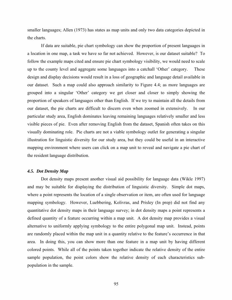
95

smaller languages; Allen (1973) has states as map units and only two data categories depicted in

the charts.

If data are suitable, pie chart symbology can show the proportion of present languages in

a location in one map, a task we have so far not achieved. However, is our dataset suitable? To

follow the example maps cited and ensure pie chart symbology visibility, we would need to scale

up to the county level and aggregate some languages into a catchall ‘Other’ category. These

design and display decisions would result in a loss of geographic and language detail available in

our dataset. Such a map could also approach similarity to Figure 4.4; as more languages are

grouped into a singular ‘Other’ category we get closer and closer to simply showing the

proportion of speakers of languages other than English. If we try to maintain all the details from

our dataset, the pie charts are difficult to discern even when zoomed in extensively. In our

particular study area, English dominates leaving remaining languages relatively smaller and less

visible pieces of pie. Even after removing English from the dataset, Spanish often takes on this

visually dominating role. Pie charts are not a viable symbology outlet for generating a singular

illustration for linguistic diversity for our study area, but they could be useful in an interactive

mapping environment where users can click on a map unit to reveal and navigate a pie chart of

the resident language distribution.

4.5. Dot Density Map

Dot density maps present another visual aid possibility for language data (Wikle 1997)

and may be suitable for displaying the distribution of linguistic diversity. Simple dot maps,

where a point represents the location of a single observation or item, are often used for language

mapping symbology. However, Luebbering, Kolivras, and Prisley (In prep) did not find any

quantitative dot density maps in their language survey; in dot density maps a point represents a

defined quantity of a feature occurring within a map unit. A dot density map provides a visual

alternative to uniformly applying symbology to the entire polygonal map unit. Instead, points

are randomly placed within the map unit in a quantity relative to the feature’s occurrence in that

area. In doing this, you can show more than one feature in a map unit by having different

colored points. While all of the points taken together indicate the relative density of the entire

sample population, the point colors show the relative density of each characteristics sub-

population in the sample.

96

Figures 4.6 and 4.7 show a compilation of dot density maps generated from the D.C.

MSA language dataset. With English and Spanish dominating the overall language composition

of the D.C. MSA, it is very difficult to show all languages within one dot density map using the

same defined feature occurrences per point (ex. 1 dot = 100 speakers). English and Spanish

would visually overwhelm the points for other languages. To avoid this, we have generated

separate dot density maps for English (Figure 4.6A) and Spanish (Figure 4.6B), maintaining the

same defined quantity for the dot symbology for both maps (1 dot = 100 speakers) and the same

dot size. The population distribution of the remaining languages in the D.C. MSA was used to

sort the language groups for the remaining two maps in Figure 4.7. All languages, other than

English and Spanish, with more than 1000 speakers form Figure 4.7A, while all languages with

less than 1000 speakers form Figure 4.7B. Given the smaller speaker populations of the

languages in Figure 4.7, the quantity representation for the dot symbology is adjusted to one dot

equaling 100 and 5 speakers, for Figure 4.7A and 4.7B respectively.

The dot density map overcomes the monolingual mapping hurdle by allowing more than

one language to appear within a map unit while also still showing a measure of quantity for each

language. It can convey the pervasiveness of major languages (Figure 4.6A), but it can also

show, if present, the clustering of smaller languages (Figure 4.7B). Dot density maps break up

the data of the census tract and show it in pieces as points. This creates a nice departure from the

one-note color shading of census tract polygons featured in Figures 4.2 through 4.5 and lessens

the emphasis on the boundaries of the census tracts (Wikle 1997). This departure from

symbology that highlights administrative boundary units is a good strategy for handling the map

unit and boundary issues discussed in the literature. However, these dot density maps are not

without their problems. There are notably so many language categories in Figure 4.7 that it

makes discerning their different representative colors rather difficult. Since we are trying to see

what is possible with this publically available dataset while using the full extent of its

information (largest scale and all languages recorded), we acknowledge this problem. This could

be solved by creating grouped language categories (by language size, relatedness, or other

chosen quality), producing more maps in the series, or having language appearance be scale-

dependent based on language population size in an interactive map environment.

97

5. Mapping with Linguistic Diversity Indices

The above maps make valid attempts at displaying linguistic diversity, but the mapping

variables fall short in providing a holistic summary of the area’s linguistic diversity. The maps

show aspects and evidence of diversity, but they do not offer a quantification of linguistic

diversity that allows viewers to readily see which places are more diverse than others. While

many language variables account for only a single component of a language environment, such

as the population of speakers of one language in an area, there are broader statistical methods

available in the literature. Linguistic diversity indices take a more overarching approach to

quantifying a language environment.

Linguistic diversity indices incorporate, at a minimum, the number of different languages

present in addition to the speaker population of each language to tabulate one value for a location

(Brougham 1981). Diversity increases in conjunction with an increase in the number of

language groups, increasing evenness among the populations of language groups, or a

combination of both. Though used for different research subjects, the diversity indices applied

for language are similar to those used in ecology. In fact, Greenberg’s A-index, a popular

linguistic index and one that we implement here, is almost identical to the commonly used

Simpson’s index for ecological diversity (Simpson 1949; Brougham 1981). Greenberg (1956)

advocates the use of linguistic diversity indices for comparison of dissimilar regions and for use

with other types of societal factors (e.g. economic, political, etc.). In his work, Greenberg

outlines eight diversity measures of increasing complexity beginning with simple proportions

among language groups and advancing to include language resemblance, bilingualism, and

polylingualism. Brougham (1981) later summarizes five additional indices (Shannon’s,

Brillouin’s, McIntosh’s, standard deviation, and Weinreich’s). Despite the presence of multiple

diversity indices, no one index has a specific advantage (McIntosh 1967; Hill 1973); each index

measures a different facet of diversity with some indices particularly sensitive to majorities,

others to rarities (Hill 1973).

Interestingly, although linguistic diversity index values are associated with spatially

defined populations (ex. a country), we have found only one work so far (Weinreich 1957) that

displays linguistic diversity indices on a map. Typically these diversity indices are presented in

tabular format (e.g. Lewis 2009), however, since they relate to geographic entities it is not a far

stretch to assign these values to locations in a GIS. Use of linguistic diversity index values as a

98

mapping variable could more succinctly illustrate the language diversity of an area than the

current prevalent method of generating multiple maps (one per language) for users to awkwardly

sift and synthesize through (e.g. Modern Language Association’s online Language Map, Modern

Language Association 2010). In an educational context, a map of linguistic diversity index

values could be very useful for the efficiency of its message. If we are trying to convey a general

idea about the presence and variation of linguistic diversity to a general audience then a singular

measure with a simple translation of values (the higher the value, the greater the diversity) could

prove very effective. Instead of showing one value pertaining to one language, the index shows

viewers the distribution of one summary value of the diversity of a language environment. The

values can translate from one location to another, allowing for easy comparison and generating

discussion. Most importantly, perhaps, mapping with linguistic diversity indices can help

overcome the issue of power and perception in language maps. A linguistic diversity index

represents the opposite end of the spectrum from monolingual mapping. In a linguistic diversity

index, everyone from whom data was collected is represented in the statistic. Although the

variable does not immediately reveal who speaks what, every speaker is counted, and every

language is a valuable component to generating a location’s diversity index value.

5.1. Methods for Calculating Linguistic Diversity Indices

With the US Census Bureau’s Special Tabulation spreadsheet, all the data needed to

calculate a basic linguistic diversity index at the census tract level is available. As mentioned

above, linguistic diversity indices vary in complexity, some based simply on language

populations, others incorporating language relationships and multilingualism. Since language

relatedness is a topic of constant debate among linguists and is beyond the aims of this research,

we employ Greenberg’s A-index (1956) that simply accounts for the languages present in an area

and the speaker population for each. Greenberg’s A-index relates to the probability that two

randomly chosen people from a population will speak a different language. Working from the

Census dataset and as an initial exercise to explore the potential utility of mapping linguistic

diversity indices, we are simply using the Census’ established categories as separate languages

despite their possible contentious nature with linguists. As a visualization study exploring the

potential utility of mapping linguistic diversity indices for educational visual aids, we

99

acknowledge and accept this potential limitation of the dataset and plan to investigate this issue

further in future research.

Greenberg’s A-index is the sum of the squared proportions of speakers of individual

languages relative to the entire population subtracted from one (Greenberg 1956). The index is

calculated using the following formula:

A = 1 - ∑ (Pi)2

where P = the proportion of the population speaking language i

and i = 1 to n, where n equals the total number of languages present in the map unit.

For example, if an area has 100 language X speakers, 200 language Y speakers, and 400

language Z speakers, the index would be calculated as such:

A = 1 – [(100/700)2 + (200/700)2 + (400/700)2)]

A = 0.571

By subtracting the sum of squares from one, the index is arranged so that a higher value equals

greater diversity. The result is a simple score for a location on a scale from 0 (no probability of

two randomly selected speakers having different mother tongues) to approaching 1. A score of 1

is mathematically impossible but hypothetically represents a situation where every speaker has a

different mother tongue. In other words, the index varies from complete homogeneity, where

every person speaks the same language (a value of 0), to increasing diversity, where there are

multiple languages with substantial speaker populations (values approaching 1). Diversity index

values for different countries in the world range from 0 (ex. North Korea, Vatican State) to as

high as 0.990 (Papua New Guinea) (Lewis 2009). The United States’ Greenberg A-index score

is 0.319 (Lewis 2009).

5.2. Linguistic Diversity Index Map – Vector Format

Figure 4.8 shows the mapped results of our calculations of Greenberg’s A-index for each

census tract in the D.C. MSA. The map was created using 10 classes established by natural

breaks except for the separate class of ‘Complete Homogeneity’ which represents tracts with an

index value of 0. The pattern seen in Figure 4.8 is not unlike some of the patterns seen in earlier

figures, however the use of a diversity index that represents all speakers makes this pattern of

linguistic diversity more definitive. Cartographically, there is no intentional deception through

design decisions as to who to include or not include (the possibility of deception stemming from

100

the dataset itself, unintentional or otherwise, is of course still an issue). The simple scale of

results from 0 to 1 with higher values representing greater diversity is intuitive and easy for map

viewers to interpret. Despite the presence of 71 different languages or language groups and a

dataset population of approximately 4.2 million residents, the linguistic diversity index distills all

the data down to simple values that allow quick comparison of one area to another. Any

interactive version of this map could offer to viewers the exact index value of each census tract

through a simple click of the mouse. While the calculation of Greenberg’s linguistic diversity

index for the entire D.C. MSA (based on the census tract data) produces a value of 0.31, the

index values for individual tracts range from 0 to 0.86. This variability could be shown in a

table, however its expression in a map provides a visual aid that linguistic diversity not only

varies throughout the D.C MSA, but varies in a spatially discernible way.

Now that we have a mapping variable that summarizes linguistic diversity for an area, we

set out to improve its educational value and utility. Wikle (1997) features a statistical surface of

Texas based on linguistic survey results; Taylor (1977) produces ‘linguistic surfaces’ of the

Ottawa-Hull area using census data (Figure 4.9). Wikle’s (1997) surface is based on the use of a

form of the word ‘night’. Taylor’s (1977) surfaces are based on the English speaking population,

the French speaking population, and the bilingual population speaking both English and French.

The figures provide a departure from typical two-dimensional language maps, using height alone

instead of other symbology to convey speakers’ location and concentration. With a focus on

individual language features or individual languages (or bilingualism of two specific languages),

Wikle’s (1997) statistical surface and Taylor’s (1977) ‘linguistic surfaces’ each show only one

component of the community’s linguistic environment or one aspect of the community’s

linguistic surface (e.g. the English surface, the French surface). Following these works,

specifically Taylor’s (1977) ‘linguistic surfaces’, if we use a linguistic diversity index as a

mapping variable instead of individual language populations, we can produce the ‘linguistic

diversity surface’ of a community.

Figure 4.10A is a 3-dimensional rendering in ArcScene of our vector linguistic diversity

map from Figure 4.8. It is our first step in approaching a ‘linguistic diversity surface’ and is

modeled after Wikle’s (1997) prism map (perspective view of a statistical surface; Cartwright,

Peterson, and Gartner 1995) of speakers in Texas. Census tracts are extruded based on their

diversity index values and, as an amendment to both Wikle and Taylor’s figures, we also use

101

color to emphasize the index values as well. Figure 4.10B presents another design possibility

where the linguistic diversity index values are represented by height while the number of

languages present in the census tract is represented by color. As a means of illustrating our

calculation of diversity, areas with tall peaks for linguistic diversity do not always have the

greatest number of languages present (burgundy color). Using both the linguistic diversity index

and the number of languages in the same map helps convey the concept of Greenberg’s A-index

for diversity; the level of diversity hinges not only on language presence but also on relative

population. In this respect, Figure 4.10B’s educational value is twofold: 1) it conveys the spatial

distribution of linguistic diversity, and 2) it conveys the concept of linguistic diversity itself. To

help orient users, we have included a vector overlay of the District of Columbia (Williams and

Ambrose 1992).

The vector 3-dimensional model of linguistic diversity is not without its flaws in design,

in creating a ‘linguistic surface’, and in overcoming some of the language mapping issues

discussed in the literature. First, as is evident in Figure 4.10, it is difficult to present an adequate

view of the 3-dimensional surface in one static image (Wikle 1997). Maps such as these are best

viewed in an interactive environment where users themselves can rotate and move the surface.

For educational applications, a screenshot of the 3d model could be put in a textbook with a

figure caption indicating a website to access an online interactive version. Figure 4.10 also does

not truly fall in the footsteps of its inspiration, the statistical and linguistic surfaces of Wikle

(1997) and Taylor (1977) respectively. While the use of a linguistic diversity index does update

their research by producing a new map type (a 3-dimensional linguistic diversity map), the figure

is not smooth and continuous in appearance like those in Figure 4.9. The census tracts are now

towering blocks with abrupt elevation changes at their boundaries. Although we have overcome

the issue of power and perception by using a diversity index that includes everyone, our map still

exhibits the issues of vector mapping for language; it is a language map of sharp divides, discrete

in nature, and based on administrative mapping units. Wikle’s (1997) statistical surface and

Taylor’s (1977) linguistic surfaces feature continuous surfaces that pair nicely with language’s

continuous nature (Breton 1991). To achieve this continuity we can convert our vector

environment to a raster format, tying our linguistic diversity index values to individual cells.

102

5.3. Linguistic Diversity Index Map – Raster Format

Conversion from a vector environment to a raster environment can result in a loss of

detail as points, lines, and polygons are converted to pixilated versions of themselves. However,

in this particular case study, we are not working with a precise dataset, nor are we making

calculations or measurements from the resulting models. We want to visually convey an idea of

linguistic diversity and its generalized spatial distribution so a loss of detail in converting to

raster, while acknowledged, does not damage our objective.

Our language dataset is based on census geography. Although we can’t undo this fact,

we can undo the stark vector appearance. To convert our vector environment to a raster

environment, we must choose an appropriate cell size. We calculated the area of our census

tracts to discern the smallest tract in our dataset. Taking the square root of the smallest census

tract’s area, we get the maximum cell size we could use for raster conversion so that even the

smallest tract will be represented by at least one cell (approximately 400 meters). This

calculation is based on the idea that the smallest census tract is perfectly square (400 x 400 m).

However, if the census tract is oddly shaped and we use 400m cells for the raster conversion, the

smallest census tract may not be represented at all. The tract’s original vector polygon may not

align with the new raster surface in a way that its value is attached to any cells. Since census

tracts vary considerably in shape, we pared down the cell size trying both 200m (Figure 4.11A)

and 300m (Figure 4.11C) cell resolutions to ensure all census tracts and their associated values

translate to the raster environment. The resulting maps (Figures 4.11A and 4.11C) do not appear

considerably different from their vector origin. The outlines of the original census tracts are

clearly visible, with sharp breaks in the color symbology indicating their edges. Keeping the end

goal in mind of producing a smooth 3-dimensional linguistic diversity surface, we smoothed the

raster surfaces by assigning cell values based on the average diversity index value of each cell’s

3x3 cell neighborhood (Figures 4.11B and 4.11D). Our vector-to-raster map makeover results in

linguistic diversity raster surfaces where the prominence of political boundaries is diminished

(Figures 4.11B and 4.11D). By averaging cell neighborhood values, we create transition areas,

as suggested by the literature, between census tracts where linguistic diversity gradually, instead

of abruptly, changes. The improved continuity of the new surfaces more closely resemble the

continuity of language than our previous vector map productions.

103

Using ArcScene, we can create 3-dimensional views of our generated raster surfaces to

complete our ‘linguistic diversity surface’ modeled after Taylor (1977) and Wikle (1997).

Figure 4.12, based on the 300m resolution filtered raster surface, shows screenshots of two

possible versions for our 3-dimensional raster linguistic diversity surface, both with a vector

boundary overlay of the District of Columbia for orientation purposes. As done with the vector

model, Figure 4.12A uses color and height to convey linguistic diversity index values, while

Figure 4.12B uses height for diversity index values paired with a color ramp showing the number

of languages present. Figure 4.12B (like Figure 4.10B) shows map users the distribution of

linguistic diversity as well as the meaning of diversity in this context. Areas with more

languages present (burgundy in color) are not always the tallest peaks on the map; linguistic

diversity accounts not just for the number of languages but the speaker populations of each

language.

With this final map in our progressive study of visualizing linguistic diversity, we have

managed to begin addressing the major language mapping concerns outlined in the literature

while exploring a new dimension for language maps. The use of a linguistic diversity index as

our mapping variable avoids the issue of power and perception by representing all language

speakers in its calculation. The use of a raster environment allows design flexibility to

ameliorate the problems posed by a vector world. Smoothing the converted raster surface

lessens the prominence of the language data being organized by political units and also creates

visible boundary transition areas. In the 3-dimensional model, this translates to having slopes

(Figure 4.12) instead of abrupt cliffs (Figure 4.10). Like its 2-dimensional counterpart (Figure

4.11), the 3-dimensional raster map (Figure 4.12) is a presentation of language continuity, not

discreteness. It does, however, face the same issue as the 3-dimensional vector map in that it is

difficult to capture in one static view and would work best if users could interactively access it

online. Also, the effectiveness of using the diversity index with the number of languages as

height and color respectively (Figure 4.12B) needs to be tested with map users.

6. Conclusions and Future Research

While aspects of linguistic diversity and its distribution can be related through text and

tables, maps can also serve as educational figures for conveying such information. Language

mapping is difficult due to the nature of the phenomena itself. However, our exploration of

104

linguistic diversity mapping possibilities with a publicly available dataset shows that many of the

problems noted in the language mapping literature can be creatively tackled. Through generating

maps modeled after commonly used themes (leading languages, speaker percentages), we found

each map displays their own piece of the linguistic diversity puzzle. Available GIS tools allow

for considerable flexibility in symbolizing these maps to convey their unique information and

perspective to viewers. Dot density maps, a quantitative mapping style rarely used with

language data (Luebbering, Kolivras, and Prisley In prep), are shown to be a viable mapping

option for speaker population data, especially as a way to de-emphasize the mapping units used

for data collection.

The application of a statistic usually reserved for tabulations and tables only (Greenberg’s

A-index for linguistic diversity) as a new mapping variable reveals that there are ways to

combine past research with present technology to produce new avenues for visualizing linguistic

diversity. The linguistic diversity index is an excellent way to summarize a location’s linguistic

diversity that avoids the cartographic conflict of whose language to represent and whose to leave

off the map. The index accounts for all languages and language speakers, translating linguistic

diversity into a numeric scale from 0 to 1 that is intuitive and easy to understand. Three-

dimensional linguistic diversity surfaces present an additional possibility for the development of

language maps for educational contexts. This visual translation of a cultural landscape presents a

different perspective to viewers and potentially a more immersive experience if encountered in a

digitally interactive environment where viewsheds and data queries are user-driven. Our

visualization study is the first language mapping effort that focuses solely on cartographically

representing linguistic diversity and we are the first to systematically implement and critique the

use of a linguistic diversity index as a mapping variable. We renew attention to language

mapping research, pushing the potential for language mapping design forward through our

implementation of contemporary tools and data to reflect our contemporary linguistic environs.

This research is just a starting point for further exploration of cartographic options for

displaying language data using GIS and other available tools. While the above maps each have

their own strengths and weaknesses, their true utility will be determined by their educational

effectiveness with map users. A future user study, with a map series similar to those constructed

above, will investigate the linguistic diversity map messages interpreted by users’ to see which

map types and symbology strategies are most effective at conveying their intended message

105

concerning language distribution. We also plan to create more sophisticated online versions of

the 3-dimensional linguistic diversity maps, complete with additional data layers, to be

implemented as teaching tools as a means of testing their utility and fit with classroom curricula.

We hope that this work will be a starting point for greater collaboration between geographers

(and/or cartographers) and linguists. If mapping is a consideration from the initial planning

stages of a project through data collection and processing, we could enhance language mapping

possibilities as well as understand how to create maps suitable for linguists’ teaching and

research needs. Time series visualizations and analysis (such as past and upcoming census

datasets, especially the upcoming availability of 2010 census data) are an option for observing

temporal and spatial changes in linguistic diversity as well. Such datasets would be good

candidates for data animation or interactive map environments for viewers. Further, GIS is just

one contemporary mapping technology with applicability for language mapping tasks. GPS,

webmapping, uncertainty visualization and analysis, and volunteered geographic information all

offer different possibilities for language data collection, interaction, analysis, and display.

Peeters (1992) states that all language map users will never be satisfied by a singular language

map. This statement is no longer a fixed limitation to language mapping as we are no longer

limited to producing only singular, static map products. If one language map will not suffice for

everyone, then we can conveniently move along with the present technological wave to produce

series of animated, interactive, and user-data-driven language maps.

106

7. References Allen, H. B. 1973. The Linguistic Atlas of the Upper Midwest. Minneapolis: University of Minnesota Press. Ambrose, J. E. 1980. Micro-scale language mapping: An experiment in Wales and Brittany. Discussion Papers in Geolinguistics 2: 1-51. Ambrose, J. E., and C. H. Williams. 1991. Language Made Visible: Representation in Geolinguistics. In Linguistic Minorities, Society and Territory, ed. C. H. Williams, 298- 314. Clevedon: Multilingual Matters, Ltd. Bab.la. 2009. World Languages. http://en.bab.la/news/world-languages.html (last accessed 16 February 2011) Bayley, R. 2004. Linguistic diversity and English language acquisition. In Language in the USA: Themes for the Twenty-first Century, eds. E. Finegan and J. R. Rickford, 268-286. Cambridge: Cambridge University Press. Breton, R. J.-L. 1991. Geolinguistics: Language dynamics and ethnolinguistic geography. Ottawa: University of Ottawa Press. -----. 1992. 'Easy Geolinguistics' and Cartographers. Discussion Papers in Geolinguistics, 19 – 21: 68-70. Brougham, J. 1981. The measurement of language diversity. Laval Univ., Quebec: Quebec International Center for Research on Bilingualism. -----. 1986. La periodicite de la geographie linguistique actuelle: essai methodologique (The periodicity of current linguistic geography: a methodological essay). Canadian Geographer 30(3): 206-216. Cartwright, W., M. P. Peterson, and G. Gartner. 1995. Multimedia Cartography. 2nd ed. New York: Springer. Dahlman, C., W. H. Renwick, and E. Bergman. 2010. Introduction to Geography: People, places, and environments. 5th ed. Upper Saddle River, New Jersey: Pearson Prentice Hall. Davis, L. M. 2000. The reliability of dialect boundaries. American Speech 75: 257-259. Farley, C., and D. Listar. 2007. The Language Quilt. Toronto Star. 30 December 2007. http://www.thestar.com/article/289637 (last accessed 16 February 2011) Fouberg, E. H., A. B. Murphy, and H. J. de Blij. 2009. Human Geography: People, Place, and Culture. 9th ed. US: John Wiley & Sons, Inc.

107

Getis, A., J. Getis, M. Bjelland, and J. D. Fellmann. 2010. Introduction to Geography. 13th ed. New York, NY: McGraw-Hill. Greenberg, J. H. 1956. The measurement of linguistic diversity. Language 32: 109-115. Hall, R. A., Jr. 1949. The linguistic position of Franco-Provencal. Language 25: 1 - 14. Heath, S.B. 1981. English in Our National Heritage. In Language in the USA, eds. C. A. Ferguson and S. B. Heath, 6-20. Cambridge: Cambridge University Press. Hill, M. O. 1973. Diversity and evenness: A unifying notation and its consequences. Ecology 54 (2): 427-432. Hoch, S., and J. J. Hayes. 2010. Geolinguistics: The incorporation of geographic information

systems and science. The Geographical Bulletin 51: 23-36. Kirk, J. M., S. Sanderson, and J. D. A. Widdowson. 1985. Introduction: Principles and practice

in linguistic geography. In Studies in linguistic geography: The dialects of English in Britain and Ireland, eds. J. M. Kirk, S. Sanderson and J. D. A. Widdowson, 1–33. London: Croom Helm.

Knox, P. L., and Marston, S. A. 2010. Human Geography: Place and Regions in Global

Context, 5th ed. Upper Saddle River, New Jersey: Pearson Prentice Hall. Kretzschmar, W. A., Jr. 1997. Generating linguistic feature maps with statistics. In Language variety in the South revisited, eds. C. Bernstein, T. Nunnally & R. Sabino, 392-416. Tuscaloosa: University of Alabama Press. Lameli, A. 2010. Linguistic atlases – traditional and modern. In Language and Space: An

international handbook of linguistic variation. Volume 1: Theories and methods, eds. P. Auer and J. E. Schmidt, 567-592. New York: De Gruyter Mouton.

Lee, J., and J. W. A. Kretzschmar. 1993. Spatial analysis of linguistic data with GIS functions.

International Journal of Geographical Information Systems 7: 541-560. Lewis, P. M. 2009. Ethnologue: Languages of the World. 16th ed. Dallas: SIL International. Lieberson, S. 1981. Language questions in censuses. In Language Diversity and Language Contact: Essays by Stanley Lieberson, ed. S. Lieberson, 281-303. Stanford, California: Stanford University Press. Luebbering, C. R. In review. Displaying the geography of language: the cartography of language maps. Submitted to The Cartographic Journal. Luebbering C., L. W. Carstensen, J. B. Campbell, and L. S. Grossman. 2008. Expanding display size and resolution for viewing geospatial data: A user study with multiple-monitor high-

108

resolution displays. Cartography and Geographic Information Science (CaGIS) 35(3): 203-219. Luebbering, C., K. Kolivras, and S. Prisley. In preparation. The lay of the language: Surveying the cartographic characteristics of language maps. Macaulay, R. K. S. 1985. Linguistic maps: Visual aid or abstract art? In Studies in linguistic

geography: The dialects of English in Britain and Ireland, eds. J. M. Kirk, S. Sanderson, and J. D. A. Widdowson, 172–186. London: Croom Helm.

Mackey, W. F. 1988. Geolinguistics: Its scope and principles. In Language in geographic

context, ed. C. H. Williams, 20-46. Philadelphia: Multilingual Matters, Ltd. Marston, S. A., P. L. Knox, D. M. Liverman, V. Del Casino, and P. Robbins 2010. World Regions in Global Context: Peoples, Place and Environments. 4th ed. Upper Saddle River, NJ: Pearson Prentice Hall. Masica, C. P. 1976. Defining a Linguistic Area: South Asia. Chicago: University of Chicago

Press. McIntosh, R. P. 1967. An index of diversity and the relation of certain concepts to diversity. Ecology 48 (3): 392-404. Modern Language Association. 2010. The Modern Language Association Language Map.

http://www.mla.org/census_main (last accessed 19 September 2010) Nieto, S., and P. Bode. 2008. Affirming Diversity: The Sociopolitical Context of Multicultural Education. 5th ed. Boston: Pearson Education, Inc. Office of Management and Budget. 2008. OMB Bulletin No. 09-01. Executive Office of the President, Office of Management and Budget, Washington, D.C. Ormeling, F. 1992. Methods and possibilities for mapping by onomasticians. Discussion Papers

in Geolinguistics 19-21: 50-67. Peeters, Y. J. D. 1992. The political importance of the visualisation of language contact.

Discussion Papers in Geolinguistics 19-21: 6-8. Rubenstein, J. M. 2010. The Cultural Landscape: An Introduction to Human Geography. 10th ed. Upper Saddle River, NJ: Pearson Prentice Hall. Simpson, E. H. 1949. Measurement of diversity. Nature 163: 688. Shin, H. B, and R. A. Kominski. 2010. Language use in the United States: 2007. U.S. Census Bureau. http://www.census.gov/prod/2010pubs/acs-12.pdf (Last accessed 8 February 2011)

109

Taylor, D. R. F. 1977. Graphic Perceptions of Language in Ottawa-Hull. The Canadian

Cartographer 14: 24-34. Trueba, H. T. 1993. Culture and Language: The ethnographic approach to the study o f learning

environments. In Language and Culture in Learning: Teaching Spanish to Native Speakers of Spanish, eds. B. J. Merino, H. T. Trueba & F. A Samaniego, 26-27. Bristol, PA: Falmer Press.

US Census Bureau. 2000. Non-English Speakers, 2000. Map Product. http://www.valpo.edu/geomet/geo/courses/geo200/language.html (last accessed 8 February 2011) -----. 2004. Special Tabulation 224 (STP224: Detailed Language Spoken at Home for Population 5 years and over). http://www.census.gov/mp/www/spectab/specialtab.html (last accessed 16 February 2011) -----. 2007. Decennial Census. http://factfinder.census.gov/jsp/saff/SAFFInfo.jsp?_lang=en&_sse=on&_content=sp4_de cennial.html&_title=Decennial+Census (last accessed 20 January 2011) -----. 2010.About Language Use. http://www.census.gov/hhes/socdemo/language/about/index.html (last accessed 8 February 2011) Weinreich, U. 1957. Functional aspects of Indian bilingualism. Word 13(2): 203-233. Wikle, T. 1997. Quantitative mapping techniques for displaying language variation and change.

In Language variety in the South revisited, eds. C. Bernstein, T. Nunnally, and R. Sabino, 417-433. Tuscaloosa: University of Alabama Press.

Wikle, T., and G. Bailey. 2010. Mapping North American English. In Language and Space: An international handbook of linguistic variation. Volume 2: Handbook to Linguistic Mapping, eds. A. Lameli, R. Kehrein, and S. Rabanus, 253-268. New York: De Gruyter Mouton. Wiley, T. G. 1996. Literacy and Language Diversity in the United States. Arlington,VA and McHenry, IL: Center for Applied Linguistics and Delta Systems. Williams, C. H. 1984. On measurement and application in geolinguistics. Discussion Papers in

Geolinguistics 8: 1-22. -----. 1988. An introduction to geolinguistics. In Language in geographic context, ed. C. H.

Williams, 1-19. Philadelphia: Multilingual Matters, Ltd. -----. 1996. Geography and contact linguistics. In Contact linguistics: An International

110

Handbook of Contemporary Research, eds. H. Goebl, P. H. Nelde, Z. Stary, and W. Wolck, 63-75. New York: Walter de Gruyter.

Williams, C. H., and J. E. Ambrose. 1988. On measuring language border areas. In Language in

geographic context, ed. C. H. Williams, 93-135. Philadelphia: Multilingual Matters, Ltd. -----. 1992. Geolinguistic Developments and Cartographic Problems. Discussion Papers in

Geolinguistics 19-21: 11-32. Williams, C. H., and I. Van der Merwe. 1996. Mapping the multilingual city: A research agenda

for urban geolinguistics. Journal of Multilingual and Multicultural Development 17: 49-66.

 

111

 

   

Figure 4.1. Study area map of Washington, D. C. Metropolitan Statistical Area.

112

 Figure 4.2. Leading language category after English by census tract in the Washington, D.C. Metropolitan Statistical Area. 

113

 Figure 4.3. Percentage of population that speaks Spanish by census tract in the Washington, D.C. Metropolitan Statistical Area.

114

   Figure 4.4. Percentage of population that speaks any language other than English by census tract in the Washington, D.C.   Metropolitan Statistical Area. 

115

   Figure 4.5. Map series showing the percentage of population, by census tract, that speaks the top ten most prevalent languages after English in the Washington, D.C. Metropolitan Statistical Area. Languages are ordered by descending speaker populations from top left to bottom right. Center map shows speakers of all languages other than English combined (modeled after Figure 4.4).

116

 

  Figure 4.6. Dot density maps of A) English speakers and B) Spanish speakers in the Washington, D.C. Metropolitan Statistical Area.

117

 Figure 4.7. Dot density maps of A) languages with > 100 speakers (excluding English and Spanish) and B) languages with < 1000 speakers in the Washington, D.C. Metropolitan Statistical Area.

118

  Figure 4.8. Vector map of linguistic diversity index values by census tract in the Washington, D.C. Metropolitan Statistical Area.

119

 A)

      B)

 Figure 4.9. Previous linguistic surfaces research by A) Wikle (1997) and B) Taylor (1977).

120

A)  

  B)

  Figure 4.10. 3-dimensional vector models of linguistic diversity index values by census tract in the Washington, D.C. Metropolitan Statistical Area using A) linguistic diversity index values for both height and color, and using B) linguistic diversity index values for height with the number of languages per census tract shown by color.  

121

  Figure 4.11. Raster maps of linguistic diversity index values by census tract for the Washington, D.C. Metropolitan Statistical Area. Maps show different resolutions and smoothing filters applied: A) 200 meter cell size, B) average filter applied to 200 meter cell size, C) 300 meter cell size, and D) average filter applied to 300 meter cell size.

122

A)

B)

  Figure 4.12. 3-dimensional raster models of linguistic diversity index values by census tract in the Washington, D.C. Metropolitan Statistical Area based on the 300m resolution filtered raster surface (Figure 4.12D) using A) linguistic diversity index values for both height and color, and using B) linguistic diversity index values for height with the number of languages per census tract shown by color.

123

Chapter 5: Conclusion

1. Conclusions

Language maps have a long history as important teaching and research tools. These

thematic maps will continue to serve that capacity especially as our linguistic environment

continues to move and change. The research presented here brings a contemporary perspective

to the task of language mapping through a comprehensive literature review and description of

current mapping efforts, a cartographic survey of language map characteristics, and exploration

of visualizing linguistic diversity through the use of GIS and linguistic diversity indices. As

language maps continue to be produced for outlets ranging from textbooks to government

publications, this research contributes to both the establishment of and progression in language

map design and construction. Three broad research gaps are filled by this dissertation: 1) a

noticeable lack of research in language mapping within the last 20 years; 2) the absence of any

documentation or quantification of language mapping symbology and design practices; and 3)

little application of GIS in language mapping research despite the literature’s recommendation to

do so.

The first manuscript chapter of this dissertation, “Displaying the geography of language:

the cartography of language maps” (Chapter 2), summarizes previous language mapping research

and describes contemporary language mapping projects as well as future research directions for

the field. Prior to this work, language mapping has been relatively unexplored since the 1980s

and 1990s. This chapter renews the conversation, presenting the research to a new audience that

is better equipped to tackle language mapping issues of the past with the mapping technology of

today. Issues such as scale, boundary representation, map units, and power are discussed in the

context of language map construction followed by an overview of the importance of and

potential for the use of computers and GIS for mapping language-related data. Discussion of

present-day language mapping efforts reinforces the relevance and vitality of this topic, while the

relative absence of GIS in language mapping work, despite researchers’ advocacy for its

application, indicates a research need (Hoch and Hayes 2010). Potential future research

directions in language mapping include the use of fuzzy membership, linguistic diversity indices,

language surfaces, and volunteered geographic information (VGI). Although language mapping

research has been mostly relegated to the past, there is enormous present-day potential to further

124

the field with the new tools we have at our disposal. This chapter sets the foundation for the

pursuit of contemporary language mapping research.

Chapter 3, “The lay of the language: surveying the cartographic characteristics of

language maps”, is the first of two manuscripts describing new original research efforts in

language mapping. As discovered through Chapter 2, there are no established guidelines, rules,

or common conventions for the difficult task of constructing a language map (Kirk, Sanderson,

and Widdowson 1985; Ambrose and Williams 1991; Williams 1996). In an effort to fill this

void, the research presented in chapter 3 is a map survey that documents language mapping

tactics in practice, summarizing the type and frequency of symbology strategies and map

components used in a large sample of 240 language maps. This is the first research to

systematically document language map characteristics through map observations and reveals

both the common approaches used by many map authors as well as the unique strategies used by

a few. Using Ambrose and Williams’ (1991) typology, the maps are consistently classified for

their overall symbology strategies and details specifically related to issues noted in the literature

are noted. The use of polygons, rather than points or lines, dominated (68% of maps), and the

most frequent symbology types were polygonal chorochromatic maps (47% of maps) or

language labels placed directly on the map (37% of maps). The results also reflect the

occurrence of the most prominent language map construction problems discussed in the

literature: boundary depiction, the use of political map units, and the visibility of linguistic

diversity. Also, unique strategies not previously discussed in the language mapping literature

were observed and fell under three general categories: visualizing linguistic diversity, indicating

data uncertainty or fluidity, and using unanchored labels. The map survey results led to the

creation of a new language map symbology typology to update Ambrose and Williams’ (1991)

work that more adequately summarizes the language mapping practices observed. This research

removes some of the mystery from the actual practice of language mapping by documenting the

common characteristics from produced language maps and also notes the prevalence of the

specific problems cited by past researchers. It also reveals the creativity and ingenuity often

displayed in language mapping as well as both the problem areas that deserve greater attention

and the possibilities for new symbology strategies.

The final manuscript of this dissertation, “Visualizing linguistic diversity through

cartography and GIS: a case study of commonly used techniques and the potential of linguistic

125

diversity index mapping” (Chapter 4), explores the specific issue of displaying linguistic

diversity through maps. This paper represents one of the few efforts in recent research to apply

GIS to a language mapping problem by specifically tackling the issue of power and perception

discussed in the literature and observed in the map survey. Using the Washington, D. C.

Metropolitan Statistical Area as the study extent coupled with publicly available census data, the

research explores both strategies in use (leading language, speaker population percentages, and

dot density mapping) as well as a new approach of using a linguistic diversity index as a

mapping variable. Linguistic diversity indices stem from the 1950s (Greenberg 1956) and

account for both the number of languages and the number of speakers of each language for a

given location summarized into one statistic. Such indices are calculated for geographic units

and therefore are natural mapping variables, yet they are typically only found listed in tables (e.g.

Lewis 2009) and were observed as a mapping variable only once in the map survey in chapter 3

(Weinreich 1957). Using the census dataset, a progression of linguistic diversity index maps are

produced ranging from vector, census tract maps to three-dimensional ‘linguistic diversity

surfaces’ following the works of Taylor (1977) and Wikle (1997). The diversity index maps

address the issue of power and perception as every speaker is represented in the value assigned to

each area. No choices are made as to whose language to represent over others. The final maps,

three-dimensional raster surfaces, more closely match the continuous nature of language while

using a new dimension (height) to convey the topography of linguistic diversity as a potential

new teaching tool. This research serves as an example of how previous language mapping issues

can be challenged with contemporary technology and creativity to produce new visualization

options for language mapping.

Overall, this dissertation renews interest and research in the area of language mapping by

not only reintroducing the literature to today’s audience and describing current language

mapping efforts, but also by providing important baseline studies documenting language

mapping trends and illustrating the potential use of GIS to move language mapping forward. In

discussing language mapping research in the context of today’s linguistic and technological

society, providing the first comprehensive survey of language mapping techniques, and applying

GIS to confront the issue of power and linguistic diversity, the presented chapters are intended to

provide a platform from which a new body of language mapping research can take off. There are

limitations to the research presented here such as the lack of linguist involvement in the work,

126

the use of the highly criticized census dataset for language, or the minimal application of GIS,

but these limitations represent just a few of the many research initiatives that will hopefully stem

from the work presented. In attempting to revive a topic that has been mostly overlooked for the

past 20 years, the foundation, importance, and potential of language mapping has to be

reestablished to garner researchers’ attention and elicit their interest. The work presented here

strives to accomplish this. The maps we produce are only as good as the datasets they represent

and therefore one of the biggest challenges in language mapping is the quality and completeness

of available data. By generating awareness for the mapping tools and possibilities available for

language data, this research can help inspire improved dataset collection that keeps language

mapping and spatial analysis in mind.

The future research possibilities from this dissertation, and in the discipline in general,

are many and varied. The immediate next steps following this research include a map user study

investigating the interpreted map messages from different language map representations as well

as creating online, interactive environments for the general public to visually explore the spatial

distribution of linguistic diversity. The difficulty of data collection pairs nicely with the

potential of volunteered geographic information (VGI) and the proliferation of user-generated

digital data. Recently a map of profanity in the US generated from tweets was featured on the

cover of Cartographic Perspectives, the journal of the North American Cartographic Information

Society (Huffman 2010). A language mapping project using VGI has the benefit of creating

large, up-to-date sample sizes while involving participants in the process. Greater collaboration

with linguists is essential for making meaningful language mapping progress and must be a high

priority for future research in this topic. The work presented here has already resulted in

generating linguist contacts eager to explore mapping options with their existing datasets.

Peeters (1992) notes that no single language map can satisfy all map users. Given the interactive

and adaptive progression of both mapping and display technology, this may no longer be an

insurmountable hurdle as our instances of being limited to just one paper map grow fewer and

farther between.

Someone recently said to me, “Language maps seem to lie more than other maps.” In

considering this statement, I think the real issue is that the generalizations made in language

maps have more personal and meaningful repercussions than the simplification liberties taken

with other map themes. Language is an aspect of human identity, and with it being so, we must

127

make an effort to map the topic as carefully and accurately as possible. This task grows

increasingly difficult as our linguistic environs increase in complexity. Yet it is that increasing

complexity and the importance of understanding its relationship to and reflectance of culture,

that makes language maps all the more valuable.

128

2. References

Ambrose, J. E., and C. H. Williams. 1991. Language Made Visible: Representation in Geolinguistics. In Linguistic Minorities, Society and Territory, ed. C. H. Williams, 298- 314. Clevedon: Multilingual Matters, Ltd. Greenberg, J. H. 1956. The measurement of linguistic diversity. Language 32: 109-115. Hoch, S., and J. J. Hayes. 2010. Geolinguistics: The incorporation of geographic information

systems and science. The Geographical Bulletin 51: 23-36. Huffman, D. P. 2010. Profane mountains. Polite plains. Cartographic Perspectives 66: cover. Kirk, J. M., S. Sanderson, and J. D. A. Widdowson. 1985. Introduction: Principles and practice

in linguistic geography. In Studies in linguistic geography: The dialects of English in Britain and Ireland, eds. J. M. Kirk, S. Sanderson and J. D. A. Widdowson, 1–33. London: Croom Helm.

Lewis, P. M. 2009. Ethnologue: Languages of the World. 16th ed. Dallas: SIL International. Peeters, Y. J. D. 1992. The political importance of the visualisation of language contact.

Discussion Papers in Geolinguistics 19-21: 6-8. Taylor, D. R. F. 1977. Graphic Perceptions of Language in Ottawa-Hull. The Canadian

Cartographer 14: 24-34. Weinreich, U. 1957. Functional aspects of Indian bilingualism. Word 13(2): 203-233. Wikle, T. 1997. Quantitative mapping techniques for displaying language variation and change.

In Language variety in the South revisited, eds. C. Bernstein, T. Nunnally, and R. Sabino, 417-433. Tuscaloosa: University of Alabama Press.

Williams, C. H. 1996. Geography and contact linguistics. In Contact linguistics: An

International Handbook of Contemporary Research, eds. H. Goebl, P. H. Nelde, Z. Stary, and W. Wolck, 63-75. New York: Walter de Gruyter.

129

Appendix A: Language Map Survey Sheet  

Language Map Survey File Name of Map Image: Publication Source of Language Map: Type (ex. textbook, website, magazine): Year: Full Citation/Website: Page # (if applicable): Map Title: Map Caption: Data Source information provided? ____ Yes ____ No If yes, note data source: Map Scale included? _____ Yes _____ No Geographic Coverage (ex. African continent): Format: _____ Vector _____ Raster If Vector, what is used to symbolize language (Check all that apply): ____ Points _____ Lines _____Polygons Color_______ Black & White_______ Map Legend Present? _____Yes ______No Language data item labels on the map? _____Yes _____No What is the language variable(s)/characteristic(s) is mapped?: What is the mapping unit (if unclear, describe)?: Are all boundaries used for language/linguistic information solid lines? _____ Yes _____ No ____ N/A Briefly explain: How many languages are mapped (# of language items in legend/# of languages labeled on the map)? What is the maximum number of languages present in one location? What is the hierarchy of language information (ex. language family – language branch – language)? What is the hierarchy of symbology used (ex. polygon fill color + label)? Describe the symbology scheme used for languages (use Ambrose & William’s 1991 language map classification scheme, add further details if needed): Symbol type details (ex. shapes for point symbols, solid or hash fill for polygons): Other data included on the map besides language: Notes: