the cauchy-kovalevskaya theorem - wordpress.com1. the cauchy-kovalevskaya theorem for odes 29...

CHAPTER 2

The Cauchy-Kovalevskaya Theorem

We shall start with a discussion of the only “general theorem” which can be ex-tended from the theory of ODEs, the Cauchy-Kovalevskaya Theorem, as it allows tointroduce the notion of principal symbol and non-characteristic data and it is importantto see from the start why analyticity is not the proper regularity for studying PDEsmost of the time.

Acknowledgements. Some parts of this chapter – in particular the four proofs of theCauchy-Kovalevskaya theorem for ODEs – are strongly inspired from the nice lecturenotes of Bruce Diver available on his webpage, and some other parts – in particular theorganisation of the proof in the PDE case and the discussion of the counter-examples– are strongly inspired from the nice lectures notes of Tsogtgerel Guntumur availableon his webpage.

1. The Cauchy-Kovalevskaya theorem for ODEs

Let us first do some recalls on the notion of real analyticity.

Definition 1.1. A function f defined on some open subset U of the real line issaid to be real analytic at a point x0 2 U if it is an infinitely di↵erentiable functionsuch that the Taylor series at the point x0

T (x) =1X

n=0

f (n)(x0)

n!(x� x0)

n(1.1)

converges (absolutely and even absolutely-uniformly) to f(x) for x in a neighborhoodof x0.

A function f is real analytic on an open set U of the real line if it is real analyticat any point x0 2 U . The set of all real analytic functions on a given open set U isoften denoted by C!(U).

Alternatively the notion of real analyticity can be understood as a growth control onthe derivatives: f is real analytic on an open set U in the real line i↵ for any compactset K ⇢ U there are constants C(K), r > 0 so that

8x 2 K, |f (n)(x)| C(K)n!

rn.

Proof of equivalence of the definitions. As it will important in this chap-ter, let us outline the proof of the equivalence of the two definitions. Assume that f isreal analytic in U in the sense of the first definition: f(x) = T (x) and T (x) absolutely-uniformly convergent in B(x0, r) ⇢ U (closed ball). We then define f(z) = T (z) forz 2 C on the ball B(x0, r) in C, which is well-defined thanks to the convergence of the

27

28 2. THE CAUCHY-KOVALEVSKAYA THEOREM

series, complex analytic, and which extends f . Then for any x 2 B(x0, r/2) \ R, wehave by Cauchy’s integral formula

f (n)(x) =n!

2⇡i |z�x0|=r

f(z)

(z � x)n+1dz

from which we deduce

maxx2B(x0,"/2)

|f (n)(x)| Cn!

rn

which is the growth control in the second alternative definition on K = B(x0, r/2).The case of a general compact K is obtained by a finite covering by such closed balls.

Conversely, let us assume the growth control on K = B(x0, r). Then for x 2B(x0, r/2), we expand f into a Taylor series around x0 at order n

f(x) =nX

k=0

f (k)(x0)(x� x0)k

k!+ f (n+1)(yn(x))

(x� x0)n+1

(n+ 1)!

for some yn(x) in B(x0, r/2). From the growth control the remainder satisfies�

�

�

�

f (n+1)(yn(x))(x� x0)n+1

(n+ 1)!

�

�

�

�

1

2n+1n!+1��! 0

and the Taylor is convergent. We deduce that on B(x0, r/2) the Taylor series is con-vergent and converges to f . ⇤

Remark 1.2. The definition of a complex analytic function is obtained by replacing,in the definitions above, “real” with “complex” and “real line” with “complex plane”.

Example 1.3. Simple examples of analytic functions (on the real line or the com-plex plane) are polynomials and the exponential and trigonometric functions. The com-plex conjugate z 7! z is not complex analytic, although the restriction to the real lineis the identity which is real analytic.

Exercise 10. Construct an example of a smooth non-analytic function on the realline. Hint: Build a non-zero smooth function with compact support.

Exercise 11. Recall the Liouville theorem for analytic function of the whole com-plex plane. Is it true on the real line? Hint: Consider the function f(x) = 1/(1 + x2).

Exercise 12. Discuss what can happen in terms of convergence, absolute conver-gence, uniform convergence, for a series like (1.1).

Finally one can extend the notion of real analyticity to the case of several realvariables. It requires the notion of power series of several variables: a power series ishere defined to be an infinite series of the form

T (x1, . . . , x`) =1X

j1,...,j`=0

aj1,...,j`Y

k=1

(xk � x0,k)jk

at the base point x0 = (x0,1, . . . , x0,`).

1. THE CAUCHY-KOVALEVSKAYA THEOREM FOR ODES 29

Definition 1.4. A function f = f(x1, . . . , x`) of ` real variables is real analytic onan open set U ⇢ R` if it is an infinitely di↵erentiable function such that at any pointx0 2 U there is a power series T in the form above, which is absolutely convergent in aneighbourhood of x0 in U , and which agrees with f in this neighbourhood.

1.1. Scalar ODEs. As a warm up we will start with the corresponding result forordinary di↵erential equations.

Theorem 1.5 (ODE Version of Cauchy–Kovalevskaya, I). Suppose b > 0 and F :(u0 � b, u0 + b) ! R is real analytic, and u(t) is the unique solution to the ODE

(1.2) u0(t) =d

dtu(t) = F (u(t)) with u(0) = u0 2 R

on some neightborhood (�a, a) of zero, with u((�a, a)) ⇢ (u0 � b, u0 + b). Then u isalso real analytic on (�a, a).

Remark 1.6. Since the construction and uniqueness of solutions, and their intervalof existence, is already settled by the Picard-Lindelof theorem, this is purely a regularitytheorem saying that the solution is real analytic in the region where the force field is.This will not be the case in the case of PDE, where the construction of solutions willbe part of the Cauchy-Kowalevskaya theorem.

We will give four proofs. However it is the last proof that the reader should focuson for understanding the PDE version of Theorem 3.1.

Observe that

• the existence and uniqueness of solutions is granted by Picard-Lindelof theo-rem;

• (however existence and uniqueness arguments could be devised using the ar-guments below as well;)

• moreover by induction the solution constructed by Picard-Lindelof can beshown to be smooth, using that if u is Ck in some open set, then F (u(t)) isCk as well by composition, and finally u0 is Ck from the di↵erential equation;

• it is enough to show the regularity in a smaller neighbourhood (�a0, a0) of0 for u, as then the argument can be performed again around any point x0where u is defined and F is analytic around u(x0;

• finally without loss of generality we can restrict to u0 = 0.

Proof 1 of Theorem 1.5. This proof is left as an exercise: go back to the proofof Picard-Lindelof theorem by fixed-point argument, and replace the real variable by acomplex variable and the real integral by a complex path integral:

un+1(z) = un+1(0) +z

0F (un(z

0)) dz0 = u0 +1

0F (un(zt))z dt

and show that the contraction property and the fixed point can be performed in thespace of holomorphic functions with the infinite norm on the function, and boundingat the same time the first derivative:

|un+1 � un|loc �

�F 0��

loc|un � un�1|loc ,

�

�u0n+1(z)�

� |F |loc .


(Just like in the real case, the Cauchy convergence of fixed point is performed on theinfinite norm without derivatives, and it is combined with a uniform bound on the firstderivative.) ⇤

Proof 2 of Theorem 1.5. We follow here the same strategy as for solving anODE by “separation of variables”. If F (0) = 0 then the solution is u = 0 which isclearly analytic and we are done. Assume F (0) 6= 0, then let us define the new function

G(y) =y

0

1

F (x)dx, y 2 (�b0, b0) ⇢ (�b, b)

which is again real analytic for b0 small enough (to make sure that F (x) does not cancelin (�b0, b0)). Then we have by the chain rule in the (possibly smaller) neighbourhood(�a0, a0) ⇢ (�a, a) where u is defined and which is mapped into the region where G isanalytic u((�a0, a0)) ⇢ (�b0, b0):

d

dt[G(u(t))] =

u(t)

F (u(t))= 1

which implies, together with G(u(0)) = G(0) = 0, that G(u(t)) = t. Finally observethat since G0(0) = 1/F (0) 6= 0, there is (�a00, a00) ⇢ (�a0, a0) where G�1 is defined andanalytic. Then u(t) = G�1(t) is analytic on (�a00, a00) which concludes the proof. ⇤

Proof 2 of Theorem 1.5. Let us consider, for z 2 C, the solution uz(t) to

(1.3) u0z(t) = zF (uz(t)), uz(0) = u0.

Then for any |z| 2, one can construct by Picard-Lindelof a solution to (1.3) on a neigh-bourhood |t| ": indeed the Lipshitz constant influences the size of the neighbourhoodbut can be uniformly bounded for |z| 2, which yields a uniform neightborhood |t| "for all |z| 2. Assume that " is also small enough so that one can construct a solutionu(t) to the original equation on |t| < 2".

(Observe that if u is real analytic, it extends to neighbourhood in the complexplane, and satisfies there the equation (1.3).)

Let us recall the notation

@

@z=

1

2

✓

@

@x� i

@

@y

◆

,@

@z=

1

2

✓

@

@x+ i

@

@y

◆

.

One can show by calculations that for any di↵erentiable solution to (1.3) in t, z (in thesense of several real variables) one has

@

@t

@uz(t)

@z= zF 0(uz(t))

@uz(t)

@z

(observe that here we have only used the chain rule, and the real di↵erentiability ofF ). This implies that

@uz(t)

@z= exp

✓ t

0zF 0(uz(s)) ds

◆

@uz(0)

@z,

which, together with the initial condition uz(0) = 0, proves that @uz(t)/@z = 0 fort 2 (�", "). These are the Cauchy-Riemann equations, and thus z 7! uz(t) is complexanalytic for any t in (�", ").


We deduce the following (convergent) power series expansion

u1(t) =1X

n=0

1n

n!

✓

@nuz(t)

@zn

◆

�

�

�

z=0.

Now observe that by uniqueness in the Picard-Lindelof theorem, we have for z 2 Rreal that u(zt) is also a solution (1.3), which implies by uniqueness uz(t) = u(zt) fort 2 (�", ") and z 2 [�2, 2], and thus

✓

@nuz(t)

@zn

◆

�

�

�

z=0=

✓

@nu(zt)

@zn

◆

�

�

�

z=0= tnu(n)(0)

which yields the convergence of the Taylor series of u at 0 on |t| < ", together with theequality

u(t) = u1(t) =1X

n=0

tn

n!u(n)(0),

which proves the real analylicity. ⇤Remark 1.7. This argument relies on extending the original equation to a contin-

uous family of equation by adding an additional parameter, this is a useful idea in themore general context of PDEs.

Proof 4 of Theorem 1.5. This is the most important proof, as it is the historicproof of A. Cauchy (improved by S. Kovalevskaya) but also because it is beautifuland this is the proof we shall use in a PDE context. This is called the “method ofmajorants”. Let us do first an a priori examination of the problem, assuming theanalyticity (actually here it could be justified by using Picard-Lindelof to contructsolutions, and then check by boostrap that this solution is C1). Then we compute thederivatives

8

>

>

>

>

>

>

<

>

>

>

>

>

>

:

u(1)(t) = F (0)(u(t)),

u(2)(t) = F (1)(u(t))u(1)(t) = F (1)(u(t))F (0)(u(t)),

u(3)(t) = F (2)(u(t))F (0)(u(t))2 + F (1)(u(t))2F (0)(u(t)),

. . .

Remark 1.8. The calculation of these polynomials is connected to a formula devisedin the 19th century by Arbogast in France and Faa di Bruno in Italy. It is now knownas Faa di Bruno’s formula and it is good to keep it in one’s analytic toolbox:

dn

dtnF (u(t)) =

X

m1+2m2+···+nmn=n

n!

m1!1!m1m2!2!m2 . . .mn!n!mnF (m1+···+mn)(u(t))

nY

j=1

⇣

u(j)(t)⌘mj

.

Now the key observation is that there are universal (in the sense of being inde-pendent of the function F ) polynomials pn with non-negative integer coe�cients, sothat

u(n)(t) = pn⇣

F (0)(u(t)), . . . , F (n�1)(u(t))⌘

.


This is proved by induction, or simply by direct use of Faa di Bruno’s formula.We deduce by monotonicity

|u(n)(0)| pn⇣

|F (0)(0)|, . . . , |F (n�1)(0)|⌘

pn⇣

G(0)(0), . . . , G(n�1)(0)⌘

for any function G with non-negative derivatives at zero and such that G(n)(0) �|F (n)(0)| for all n � 0. Such a function is called a majorant function of F .

But for such a function G the RHS in the previous equation is exactly

pn⇣

G(0)(0), . . . , G(n�1)(0)⌘

= v(n)(0) = |v(n)(0)|

where v solves the auxiliary equation

v0(t) =d

dtv(t) = G(v(t)), v(0) = 0.

Observe that as a consequence of the inequalities between G and F we have v(n)(0) �|u(n)(0)| for any n � 0. Hence if v is analytic near zero, the series

Sv(t) :=X

n�0

v(n)(0)tn

n!

has a positive radius of convergence and by comparison so does the series

Su(t) :=X

n�0

|u(n)(0)| tn

n!,

which shows the analyticity near zero and concludes the proof.We finally need to construct the majorant function G. From the analyticity of F

we have

8n � 0, |F (n)(0)| Cn!

rn

uniformly in n � 0, for some some constant C > 0 and some r > 0 smaller than theradius of convergence of the series, and we then consider

G(z) := C1X

n=0

⇣z

r

⌘n= C

1

1� z/r=

Cr

r � z

which is analytic on the ball centred at zero with radius r > 0. Since G(n)(0) = Cn!/rn

we have clearly the majoration G(n)(0) � |F (n)(0)| for all n � 0.To conclude the proof we need finally to compute the solution v to the auxiliary

equation

v0(t) = G(v(t)) =Cr

r � v(t), v(0) = 0,

which can be solved by usual real di↵erential calculus, using separation of variables:

(r � v) dv = Cr dt =) � d(r � v)2 = 2Cr dt =) v(t) = r ± r

r

1� 2Ct

r

and using the initial condition v(0) = 0 one finally finds

v(t) = r � r

r

1� 2Ct

r


which is analytic for |t| r/(2C).This hence shows that the radius of convergence of Sv(t) is positive, which implies

the growth control

8n � 1, 0 v(n)(0) Cn!

"nand in turn implies the growth control

8n � 1, 0 |u(n)(0)| Cn!

"n.

Since this argument can be performed uniformly for any t 2 [�a0, a0] ⇢ (�a, a), usingthe uniform growth control on the derivatives of f on the region u([�a0, a0]), we deduced

8 t 2 [�a0, a0], 8n � 1, 0 |u(n)(t)| Cn!

"n.

This shows the real analyticity (second definition). ⇤Observe the profound idea in this last proof:

• first one uncovers a general combinatorial structure at a universal level (notdepending on F defining the ODE),

• then instead of coping with the combinatorial explosion in the calculation ofthe derivatives (due to the nonlinearity), one uses a monotonicity propertyencoded in the abstract structure to reduce the control to be established to acomparison with a simpler function,

• then one goes back to the equation to deduce the analytic control, withoutever computing the derivatives.

1.2. Systems of ODEs. We now consider the extension of this theorem to sys-tems of di↵erential equations.

Theorem 1.9 (ODE Version of Cauchy–Kovalevskaya, II). Suppose b > 0 andF : u0 + (b, b)m ! Rm, m 2 N is real analytic near and u(t) is the unique solution tothe system of ODEs

(1.4)d

dtu(t) = F(u(t)) with u(0) = u0 2 Rm

on (�a, a) with u((�a, a)) ⇢ u0 + (b, b)m.Then u is also real analytic in (�a, a).

Proofs of Theorem 1.9. All but the second proof of Theorem 1.5 can be adaptedto cover this case of systems.

Exercise 13. Extend the proofs 1 and 3 to this case.

Let us give some more comments-exercises on the extension of the last proof, themethod of majorants.

Exercise 14. Suppose F : (�a, a)m ! Rm is real analytic near 0 2 (�a, a)m, provethat a majorant function is provided by

G(z1, . . . , zm) := (G1, . . . , Gm), G1 = · · · = Gm =Cr

r � z1 � · · ·� zmfor well-chosen values of the constants r, C > 0.


With this auxiliary result at hand, check that one can reduce the proof to provingthe local analyticity of the solution to the system of ODE:

d

dtv(t) = G(v(t)), v(t) = (v1(t), . . . , vm(t)), v(0) = 0.

Exercise 15. Prove that by symmetry one has vj(t) = v1(t) =: w(t) for all 1 j m, and that w(t) solves the scalar ODE

d

dtw(t) =

Cr

r �mw(t), w(0) = 0

so that w(t) = (r/m)(1�p

1� 2Cdt/r).

With the two last results it is easy to conclude the proof. ⇤

2. The analytic Cauchy problem in PDEs

We consider a k-th order scalar quasilinear PDE1

(2.1)X

|↵|=k

a↵(rk�1u, . . . , u, x)@↵xu+ a0(rk�1u, . . . , u, x) = 0, x 2 U ⇢ R`

whererju :=

⇣

@xi1. . . @xij

u⌘

1i1,...,ij`, j 2 N,

is the j-th iterated gradient, and

@↵x := @↵1x1

. . . @↵`x`

for a multi-index ↵ = (↵1, . . . ,↵`) 2 N`, and U is some open region in R` (` � 2 is thenumber of variables), and u : U ! R.

Remark 2.1. The word “quasilinear” relates to the fact that the coe�cient of thehighest-order derivatives only depend on derivatives with strictly lower order. Theequation would be semilinear if a↵ = a↵(x) does not depend on u and the nonlinearityis only in a0. The equation is linear when of course both a↵ and a0 do not depend onu, and it is a constant coe�cient linear equation when a↵ and a0 do not depend on xeither.

We consider a smooth (` � 1)-dimensional hypersurface � in U , equiped with asmooth unit normal vector n(x) = (n1(x), . . . , n`(x)) for x 2 �.

Remark 2.2. We will discuss this more in details, but let us make precise themeaning of �. This is an embedded smooth submanifold of R` with dimension (`� 1).This means that around any point x 2 � there a smooth non-singular bijective map x : B`(0, ") ⇢ Rd ! Vx ⇢ U with x(B`(0, ")\ {y` = 0}) = �\Vx, and Vx some openneighbourhood of x in U . The collection of all such pairs (Vx, x) of neighbourhood andapplications (called charts) forms an atlas.

1Actually when k = 1 (first order) another simpler proof than the one we shall do here can beperformed by the so-called characteristics method (see chapter 5 where we will come back to this).This method can be understood as the natural extension of the ODE arguments in proofs 1-2-3 aboveusing trajectories for the PDE. However this method fails for systems, and therefore is unable to treatk-th order PDEs as we shall see, which justifies the need for a more general proof.

2. THE ANALYTIC CAUCHY PROBLEM IN PDES 35

The smooth unit normal vector map is a smooth map when composed locally withthe charts, and which is orthogonal at each point to the tangent hyperplane obtained bythe chart. This tangent plan at a point x = x(0) is the a�ne vector hyperplane

Tx = x+ Span

✓

@

@y1(0), . . . ,

@

@y`�1(0)

◆

.

Observe that from this definition one has also:(1) Locally in a neighbourhood of any point x 2 �, by restriction of x, we have an

application x : B`�1(0, ") ! (Vx \ �) ⇢ U ⇢ R`, that is again smooth from R`�1 toR`.

(2) By constructing then (y) = x(y) + ⇤(y)n( x(y)) we obtain a smooth chartwith y = (y1, . . . , y`�1) and �(y) 6= 0 on ⇥, and with

@

@y`(y) =

@⇤

@y`(y)n(y) = �(y)n(y)

(3) Observe that scalar smooth non-degenerate function ' = �` : Ux ! R satisfies� \ Ux = {' = 0}, and the normal vector n(x) is colinear to rx'(x).

(4) Then by adjusting �(y) = @⇤/@y` (tangential speed) we can modify the normof rx�` so that n(x) = rx'(x) = rx�`(x). The key observation is that

1 =h

fct of �1, . . . , �`�1 and ⇤, @1⇤, . . . , @`�1⇤i

+@⇤

@y`

@�`

@xini =

h

. . .i

+ �@i'ni

and by rescaling y` ! Cy` we can obtain the desired parametrisation.This is part of the di↵erential geometry course, although we will not need more than

what is introduced in this chapter in this matter.

We then define the j-th normal derivative (for j 2 N) of u at x 2 � as

@ju

@nj:=

X

|↵|=j

r↵xu : n↵ =

X

|↵|=j

@↵u

@↵xn↵ =

X

↵1+···+↵`=j

@ju

@x↵11 . . . @x↵`

`

n↵11 . . . n↵`

` .

Now let g0, . . . , gk�1 : �! R be k given functions on �, and x0 2 �. The Cauchyproblem is then to find a function u solving (2.1) in some open set including x0,subject to the boundary conditions

(2.2) u = g0,@u

@n= g1, . . . ,

@k�1u

@nk�1= gk�1, x 2 �.

We say that the equation (2.2) prescribes the Cauchy data g0, . . . , gk�1 on �.If one wants to compute an entire series for the solution, certainly all the derivatives

have to be determined from equations (2.1)-(2.2). In particular all partial derivativesof u on � should be computed from the boundary data (2.2).

The basic question is now: assuming first that we have a smooth solution and leav-ing aside the question of the convergence of the Taylor series, what kind of conditionsdo we need on � in order to so?


2.1. The case of a flat boundary. In order to gain intuition into the problem,we first examine the case where U = R` and � = {x` = 0} is a vector hyperplan.We hence have n = e` (the `-th unit vector of the canonical basis) and the boundaryprescriptions (2.2) read

u = g0,@u

@x`= g1, . . . ,

@k�1u

@xk�1`

= gk�1, x 2 �.

Which further partial derivatives can we compute on the hyperplan �? First sinceu = g0 on � by di↵erentiating tangentially we get that

@u

@xi=@g0@xi

, 1 i `� 1

is prescribed by the boundary data. Since we also know from (2.2) that

@u

@x`= g1

we can determine the full gradient on �. Similarly we can calculate inductively

@↵

@x↵

@ju

@xj`=

@↵

@x↵gj , ↵ = (↵1, . . . ,↵`�1, 0), |↵i| k� 1 for 1 i `� 1, 0 j k� 1.

(Remark that actually the ↵i in the previous equation could be taken in N.) Thedi�culty now, in order to compute the k-th derivative, is to compute the k-th ordernormal derivative

@ku

@xk`We now shall use the PDE in order to overcome this obstacle. Observe that if thecoe�cient a↵ with ↵ = (0, . . . , 0, k) is non-zero on �:

A(x) := a(0,...,0,k)(rk�1u, . . . , u, x)

= Function(gk�1(x), gk�2(x), . . . , g0(x), x) 6= 0, x 2 �,(observe that it only depends on the boundary data) then we can compute for x 2 �

@ku

@xk`= � 1

A(x)

2

4

X

|↵|=k, ↵`k�1

a↵(rk�1u, . . . , u, x)@↵xu+ a0(Dk�1u, . . . , u, x)

3

5

(where u and its derivative implicitely depend on x, although we omit it for concisenessof the formula) where the coe�cients in the RHS again only depend on the boundarydata by the previous calculations, and consequently we can therefore compute rku on�.

Definition 2.3. We say that the hypersurface � = {x` = 0} and boundary con-ditions g0, . . . , gk�1 are non-characteristics for the PDE (2.1) if the function A(x) =a(0,...,0,k)(rk�1u, . . . , u, x) never cancels on �.

Now the question is: can we calculate still higher derivatives on �, assuming ofcourse this non-degeneracy condition? The answer is yes, here is a concise inductiveway of iterating the argument:


Let us denote

gk(x) :=@ku

@xk`= � 1

A(x)

2

4

X

|↵|=k, ↵`k�1

a↵@↵xu+ a0

3

5 , x 2 �,

as computed before. We now di↵erentiate the equation along x` (we already know howto compute all the derivatives along the other coordinates, provided we have less thank derivatives along x`), which results into a new equation

X

|↵|=k

a↵(rk�1u, . . . , u, x)@↵x @x`u+ a0(rku, . . . , u, x) = 0, x 2 U ⇢ R`,

with

a0(rku, . . . , u, x) = @x`

2

4

X

|↵|=k

a↵(rk�1u, . . . , u, x)

3

5 @↵xu+ @x`

h

a0(rk�1u, . . . , u, x)i

,

which results following the same argument into

gk+1(x) :=@k+1u

@xk+1`

= � 1

A(x)

2

4

X

|↵|=k, ↵`k�1

a↵(rk�1u, . . . , u, x)@↵x @x`u+ a0(rku, . . . , u, x)

3

5

(observe that the RHS only involves derivatives in x` of order less than k), which allowsto calculate the k+1-derivative in x` from the boundary data. One can then continueinductively and calculate all derivatives.

2.2. General hypersurfaces. We shall now generalize the results and definitionsabove to the general case, when � is a smooth hypersurface with normal vector field n.

Definition 2.4. We say that the hypersurface � and boundary conditions g0, . . . , gk�1

are non-characteristic for the PDE (2.1) if

A(x) :=X

|↵|=k

a↵(rk�1u, . . . , u, x)n↵(x) 6= 0, x 2 �

(where the RHS only depends on the boundary data).

Let us prove the theorem corresponding the calculation of the partial derivatives

Theorem 2.5 (Cauchy data and non-characteristic surfaces). Assume that � issmooth and non-characteristic for the PDE (2.1) and boundary data (2.2). Then if uis a C1 solution to (2.1) with the boundary data (2.2), we can uniquely compute allthe partial derivatives of u on � in terms of �, the functions g0, . . . , gk�1, and thecoe�cients a↵, a0.

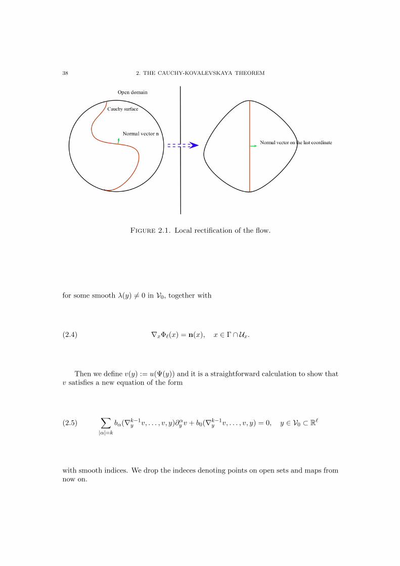
Proof of Theorem 2.5. We consider a base point x 2 � and using the previousdiscussion we find C1 maps �, defined on open sets Ux and V0 of R` so that

�(� \B(x, r)) = ⇥ ⇢ {y` = 0}, �(x) = y, = ��1

where ⇥ is the new Cauchy surface in the new coordinates, and with the two properties

(2.3)@

@y`(y) = �(y)m(y) and m(y) = n( (y, 0)) = m(y1, . . . , y`�1), y 2 V0


Figure 2.1. Local rectification of the flow.

for some smooth �(y) 6= 0 in V0, together with

(2.4) rx�`(x) = n(x), x 2 � \ Ux.

Then we define v(y) := u( (y)) and it is a straightforward calculation to show thatv satisfies a new equation of the form

(2.5)X

|↵|=k

b↵(rk�1y v, . . . , v, y)@↵y v + b0(rk�1

y v, . . . , v, y) = 0, y 2 V0 ⇢ R`

with smooth indices. We drop the indeces denoting points on open sets and maps fromnow on.


The new boundary data are (for y 2 ⇥ = {y` = 0} \ V0)8

>

>

>

>

>

>

>

>

>

>

>

>

>

>

>

>

>

>

>

>

>

>

>

>

>

>

>

>

>

>

>

>

>

>

>

>

>

>

>

>

<

>

>

>

>

>

>

>

>

>

>

>

>

>

>

>

>

>

>

>

>

>

>

>

>

>

>

>

>

>

>

>

>

>

>

>

>

>

>

>

>

:

v(y) = g0( (y)) =: h0(y),

@v

@y`(y) = (rxu)( (y))

@

@y`(y)

= �(y)@u

@n( (y)) = �(y)g1( (y)) =: h1(y),

@2v

@y2`(y) = (r2

xu)( (y)) :

✓

@

@y`(y)

◆⌦2

+@�

@y`g1( (y))

= �(y)2@2u

@n2( (y)) +

@�

@y`g1( (y))

= �(y)2g2( (y)) +@�

@y`g1( (y)) =: h2(y)

@3v

@y3`(y) = · · · =: h3(y)

.

.

.

@k�1v

@yk�1`

(y) = · · · =: hk�1(y)

where we have used repeatedly the first condition (2.3) we have imposed on our recti-fication map, and one checks by induction that they can be computed only in terms ofthe boundary conditions.

Then we want to impose the non-characteristic property in the new coordinates onthe new Cauchy surface that we have computed in the flat case in the previous section:

b(0,...,0,k)(rk�1y v, . . . , v, y) 6= 0, y 2 ⇥.

Let us compute it more precisely.Indeed we calculate with the chain rule on u = v �� = v(�1(x), . . . ,�`(x)) that for

|↵| = k and x 2 �, we have

@↵u

@x↵(x) =

@kv

@yk`(y) (rx�`(x))

↵+ lower order terms =@kv

@yk`(y)n↵(x)+ lower order terms

where the lower-order terms only involve partial derivatives with order less than k � 1in y`, and where we have used the second condition (2.4) we have imposed on ourrectification map. The other derivatives with |↵| < k only create terms involvingpartial derivatives with order less than k � 1 in y`. We hence deduce that

b(0,...,0,k)(rk�1y v, . . . , v, y) =

X

|↵|=k

a↵(rk�1x u � (y), . . . , u � (y), x)n↵( (y))


and the non-characteristic condition reads in the original parametrisation

A(x) :=X

|↵|=k

a↵(rk�1x u, . . . , u, x)n↵(x) 6= 0, x 2 �.

Exercise 16. Redo carefully the previous calculation.

From the assumption of the theorem we therefore satisfy the definition of a non-characteristic surface in the rectified parametrisation. Then using the previous caseof a flat boundary we can compute all derivatives of v, and then all derivatives of u,which concludes the proof. ⇤

Remark 2.6. The choice of the conditions imposed on the rectification map is im-portant in this proof. The condition (2.3) is not the simplest one in terms of simplicityof the new boundary data, but the second condition (2.4) simplifies the computationof the new non-characteristic condition. The final non-characteristic statement is ofcourse intrinsic to � and g0, . . . , gk�1 and the original PDE and should not depend onthe choice of the rectification.

Exercise 17. Check that all the results in this section are still valid for systemsof PDEs, when imposing boundary data as above on each coordinate of the solutionu = (u1, . . . , um).

3. The Cauchy-Kovalevskaya Theorem for PDEs

We shall now prove the following result:

Theorem 3.1 (Cauchy-Kovalevakaya Theorem for PDEs). We now consider anreal analytic Cauchy surface � in an open set U . Under real analyticity assumptionson all coe�cients U and boundary data functions in �, and the non-characteristiccondition, there is a unique local analytic solution u to the equations (2.1)-(2.2). Thismeans that for any x 2 � ⇢ U , there is Ux ⇢ U an open set including x so that thereis a unique analytic solution u to (2.1) on Ux satisfying the boundary data (2.2) on� \ Ux.

Remark 3.2. The meaning of a real analytic hypersurface is: it is implicitly definedby an analytic function ': � = {' = 0}, or equivalently it is locally rectifiable withanalytic maps �, as before. One can check that it is still possible to make theconstruction of a real analytic rectification with the two conditions imposed before bythe same arguments.

This result was first proved by A. Cauchy in 1842 on first order quasilinear evolu-tion equations, and formulated in its most general form by S. Kovalevskaya in 1874.At about the same time, G. Darboux also reached similar results, although with lessgenerality than Kovalevskaya’s work. Both Kovalevskaya’s and Darboux’s papers werepublished in 1875, and the proof was later simplified by E. Goursat in his influen-tial calculus texts around 1900. Nowadays these results are collectively known as theCauchy-Kovalevskaya Theorem.

3. THE CAUCHY-KOVALEVSKAYA THEOREM FOR PDES 41

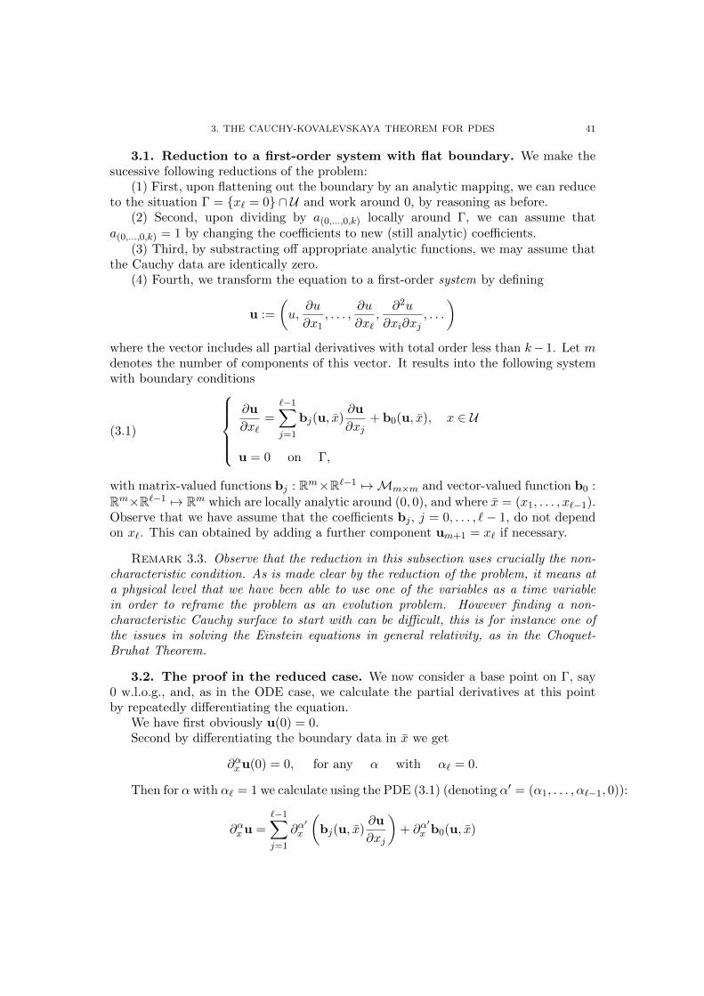
3.1. Reduction to a first-order system with flat boundary. We make thesucessive following reductions of the problem:

(1) First, upon flattening out the boundary by an analytic mapping, we can reduceto the situation � = {x` = 0} \ U and work around 0, by reasoning as before.

(2) Second, upon dividing by a(0,...,0,k) locally around �, we can assume thata(0,...,0,k) = 1 by changing the coe�cients to new (still analytic) coe�cients.

(3) Third, by substracting o↵ appropriate analytic functions, we may assume thatthe Cauchy data are identically zero.

(4) Fourth, we transform the equation to a first-order system by defining

u :=

✓

u,@u

@x1, . . . ,

@u

@x`,@2u

@xi@xj, . . .

◆

where the vector includes all partial derivatives with total order less than k� 1. Let mdenotes the number of components of this vector. It results into the following systemwith boundary conditions

(3.1)

8

>

>

>

<

>

>

>

:

@u

@x`=

`�1X

j=1

bj(u, x)@u

@xj+ b0(u, x), x 2 U

u = 0 on �,

with matrix-valued functions bj : Rm⇥R`�1 7! Mm⇥m and vector-valued function b0 :Rm⇥R`�1 7! Rm which are locally analytic around (0, 0), and where x = (x1, . . . , x`�1).Observe that we have assume that the coe�cients bj , j = 0, . . . , `� 1, do not dependon x`. This can obtained by adding a further component um+1 = x` if necessary.

Remark 3.3. Observe that the reduction in this subsection uses crucially the non-characteristic condition. As is made clear by the reduction of the problem, it means ata physical level that we have been able to use one of the variables as a time variablein order to reframe the problem as an evolution problem. However finding a non-characteristic Cauchy surface to start with can be di�cult, this is for instance one ofthe issues in solving the Einstein equations in general relativity, as in the Choquet-Bruhat Theorem.

3.2. The proof in the reduced case. We now consider a base point on �, say0 w.l.o.g., and, as in the ODE case, we calculate the partial derivatives at this pointby repeatedly di↵erentiating the equation.

We have first obviously u(0) = 0.Second by di↵erentiating the boundary data in x we get

@↵xu(0) = 0, for any ↵ with ↵` = 0.

Then for ↵ with ↵` = 1 we calculate using the PDE (3.1) (denoting ↵0 = (↵1, . . . ,↵`�1, 0)):

@↵xu =`�1X

j=1

@↵0

x

✓

bj(u, x)@u

@xj

◆

+ @↵0

x b0(u, x)


which yields at x = 0 (using the previous step):

@↵xu(0) = 0 +⇣

@↵0

x b0(u, x)⌘

�

�x=0=

⇣

D↵02 b0

⌘

(0, 0)

where D2 means the partial derivatives according the second argument of b0.Then for ↵ with ↵` = 2 we calculate again (denoting ↵0 = (↵1, . . . ,↵`�1, 1)):

@↵xu =`�1X

j=1

@↵0

x

✓

bj(u, x0)@u

@xj

◆

+ @↵0

x b0(u, x0)

which yields at x = 0:

@↵xu(0) = · · · = polynomial(@bj(0, 0), @u(0))

where is in the RHS it only involves derivatives of u with ↵` 1, which then can beexpressed in terms of derivatives of bj again.

We can continue the calculation inductively, and prove by induction that there areuniversal (independent of u) polynomials with integer non-negative coe�cients so that

@↵ui

@x↵= p↵,i

⇣

D�2bj(0, 0), |�| |↵|� 1, 0 j `� 1

⌘

.

This means: (1) all derivatives at the Cauchy hypersurface can be determinedthanks to the coe�cients and boundary data (here zeros), (2) we can amplify the ideaof Cauchy to provide bounds on these derivatives.

Unlike the case of ODEs we do not have a priori a solution to the PDE. We thusdefine the Taylor series

u(x1, . . . , x`) =X

↵�0

x↵

↵!@↵xu(0), x↵ := x↵1

1 . . . x↵`` , ↵! := ↵1! . . .↵`!(3.2)

If the radius of convergence of the entire series is non-zero, then it defines a real analyticfunction in some open set U0 including zero, which satisfies all the previous equationson the derivatives at zero. Moreover the PDE can be rewritten by composition of realanalytic functions as another entire series

@u

@x`�

`�1X

j=1

bj(u, x)@u

@xj+ b0(u, x) =: H(x) =

X

↵�0

x↵

↵!h↵

for some coe↵ecients h↵ 2 R, with a non-zero radius of convergence. Hence by reducingif necessary the open set, we have in U0 that (1) u is defined by the previous Taylorseries, and (2) the equation writes H(x) = 0 with some well-defined real analyticfunction H(x). But from the previous equations for the derivatives at zero, we haveh↵ = 0 for all ↵ � 0, and therefore H(x) = 0 in the open set. We hence deduce that usatisfies the PDE in U0.

It remains therefore to prove that the initial Taylor series for u has a non-zeroradius of convergence. We perform then the same argument as for ODEs with themajorant function

b⇤j =

Cr

r � (x1 + . . . x`�1)� (z1 + · · ·+ zm)M1, j = 1, . . . , `� 1,

3. THE CAUCHY-KOVALEVSKAYA THEOREM FOR PDES 43

where M1 is the m⇥m-matrix with 1 in all entries, and

b⇤0 =

Cr

r � (x1 + . . . x`�1)� (z1 + · · ·+ zm)U1

where U1 is the m-vector with 1 in all entries, resulting in the solution

v =1

m`(r � (x1 + · · ·+ x`�1))�

h

(r � (x1 + · · ·+ x`�1))2 � 2m`Crx`

i1/2U1

which yields the analyticity in all variables by using the growth condition characteri-sation of analyticity.

Let us decompose this last calculations into several steps, given in exercises.

Exercise 18. Using the exercise 14 on all entries of bj, j = 0, . . . , ` � 1 (whichdepend on m+ `� 1 variables), find C, r > 0 so that

g(z1, . . . , zm, x1, . . . , x`�1) =Cr

r � (x1 + . . . x`�1)� (z1 + · · ·+ zm)

is a majorant of all these entries.

Exercise 19. Defining b⇤j = gM1, j = 1, . . . , `� 1, and b⇤

0 = gU1, check that thesolution v = (v1, . . . , vm) to

8

>

>

>

<

>

>

>

:

@v

@x`=

`�1X

j=1

b⇤j (v, x

0)@u

@xj+ b⇤

0(v, x0)

v = 0 on �,

can be searched in the form v1 = · · · = vm =: w, and

w = w(x1 + x2 + · · ·+ x`�1, x`) = w(⇠, x`), ⇠ := x1 + · · ·+ x`�1.

Then it reduces the problem to solving the following scalar simple transport equa-tion (relabeling x` = t for conveniency)

(3.3) @tw =Cr

r � ⇠ � �1w(�2@⇠w + 1) , w(⇠, 0) = 0, t, ⇠ 2 R.

Exercise 20. Show that the w defining the solution v to the majorant problemabove satisfies the equation (3.3) with �2 = (`� 1)m and �1 = m.

Finally we can solve the equation (3.3) by the so-called characteristic method (whichwe shall study in much more details in the chapter on hyperbolic equations). Let ussketch the method in this case: if we can find ⇠(t) and ⌘(t) solving

8

>

>

>

<

>

>

>

:

⇠0(t) =�Cr�2

r � ⇠(t)� �1⌘(t), ⇠(0) = ⇠0,

⌘0(t) =Cr

r � ⇠(t)� �1⌘(t), ⌘(0) = ⌘0,

then if we set ⌘0 = 0 and now define w(⇠, t) by the implicit formula w(⇠(t), t) = ⌘(t),it solves by the chain-rule

⌘0(t) = (@tw)(⇠(t), t) + ⇠0(t)(@⇠w)(⇠(t), t) =Cr

r � ⇠(t)� �1⌘(t)


which writes

(@tw)(⇠(t), t)�Cr�2

r � ⇠ � �1w(⇠(t), t)(@⇠w)(⇠(t), t) =

Cr

r � ⇠(t)� �1w(⇠(t), t)

with the initial data w(⇠0, 0) = ⌘0 = 0. This is exactly the desired equation at thepoint (t, y(t)). Hence as long as the map ⇠0 7! ⇠(t) is invertible and smooth, we havea solution to the original PDE problem.2

Therefore let us solve locally in time the ODEs for ⇠(t) and ⌘(t). Since obviously⇠0(t) + �2⌘0(t) = 0, we deduce the key a priori relation

8 t � 0, ⇠(t) + �2⌘(t) = ⇠0.

Whe thus replace ⇠(t) in the ODE for ⌘(t):

⌘0(t) =Cr

r � ⇠0 + (�2 � �1)⌘(t), ⌘(0) = 0.

Here observe that �2 � �1 (remember that ` � 2). If �1 = �2 then

w(⇠(t), t) = ⌘(t) =Crt

r � ⇠0, ⇠(t) = ⇠0 �

C�2rt

r � ⇠0

which provides analyticity of the solution and concludes the proof. If (�2 � �1) =(`� 2)m > 0, then we calculate (using ⌘(0) = 0 to decide on the root)

⌘(t) = w(⇠(t), t) =1

�1 + �2

⇣

(r � ⇠(t))�p

(r � ⇠(t))2 � 2(�1 + �2)Crt⌘

which gives

w(⇠, t) =1

`m

⇣

(r � ⇠)�p

(r � ⇠)2 � 2`mCrt⌘

and concludes the proof.

Exercise 21. Check that the previous formula for w indeed provides a solution.

4. Examples, counter-examples, and classification

4.1. Failure of the Cauchy-Kovalevaskaya Theorem and evolution prob-lems. If we consider the heat equation with initial conditions (this counter-example isdue to S. Kovalevskaya)

@tu = @2xu, u = u(t, x), (t, x) 2 R2

around the point (0, 0), with the initial condition

u(0, x) = g(x)

we have, in the previous setting, � = {t = 0}, and the normal unit vector in R2 issimply (1, 0) = e1. The non-characteristic condition writes ak,0 6= 0, where k is theorder of the equation (here k = 2), which is not true here (independently of the choiceof the boundary data g). Hence the initial value problem for the heat equation is alwayscharacteristic. This reflects the fact that the equation cannot be reversed in time, or in

2The first time where this maps stops being invertible is called a caustic of shock wave dependingon the context, and will be studied in details in the chapter on hyperbolic equations.

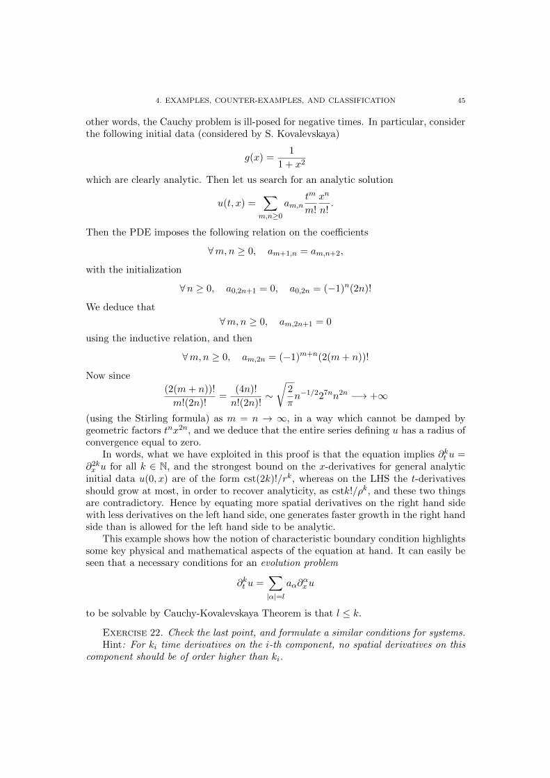
4. EXAMPLES, COUNTER-EXAMPLES, AND CLASSIFICATION 45

other words, the Cauchy problem is ill-posed for negative times. In particular, considerthe following initial data (considered by S. Kovalevskaya)

g(x) =1

1 + x2

which are clearly analytic. Then let us search for an analytic solution

u(t, x) =X

m,n�0

am,ntm

m!

xn

n!.

Then the PDE imposes the following relation on the coe�cients

8m,n � 0, am+1,n = am,n+2,

with the initialization

8n � 0, a0,2n+1 = 0, a0,2n = (�1)n(2n)!

We deduce that

8m,n � 0, am,2n+1 = 0

using the inductive relation, and then

8m,n � 0, am,2n = (�1)m+n(2(m+ n))!

Now since(2(m+ n))!

m!(2n)!=

(4n)!

n!(2n)!⇠

r

2

⇡n�1/227nn2n �! +1

(using the Stirling formula) as m = n ! 1, in a way which cannot be damped bygeometric factors tnx2n, and we deduce that the entire series defining u has a radius ofconvergence equal to zero.

In words, what we have exploited in this proof is that the equation implies @kt u =@2kx u for all k 2 N, and the strongest bound on the x-derivatives for general analyticinitial data u(0, x) are of the form cst(2k)!/rk, whereas on the LHS the t-derivativesshould grow at most, in order to recover analyticity, as cstk!/⇢k, and these two thingsare contradictory. Hence by equating more spatial derivatives on the right hand sidewith less derivatives on the left hand side, one generates faster growth in the right handside than is allowed for the left hand side to be analytic.

This example shows how the notion of characteristic boundary condition highlightssome key physical and mathematical aspects of the equation at hand. It can easily beseen that a necessary conditions for an evolution problem

@kt u =X

|↵|=l

a↵@↵xu

to be solvable by Cauchy-Kovalevskaya Theorem is that l k.

Exercise 22. Check the last point, and formulate a similar conditions for systems.Hint: For ki time derivatives on the i-th component, no spatial derivatives on this

component should be of order higher than ki.


4.2. Principal symbol and characteristic form. Let P be a scalar linear dif-ferential operator of order k:

Pu :=X

|↵|k

a↵(x)@↵xu, u = u(x), x 2 R`.

For convenience let us assume here that the a↵(x) are smooth functions.Then the total symbol of the operator is defined as

�(x, ⇠) :=X

|↵|k

a↵(x)⇠↵, ⇠↵ := ⇠↵1

1 . . . ⇠↵``

and the principal symbol of the operator is defined as

�p(x, ⇠) :=X

|↵|=k

a↵(x)⇠↵,

where ⇠ 2 C. This principal symbol is also called the characteristic form of the equa-tion.

Remark 4.1. For geometric PDEs in an open set U of some manifold M, theprincipal symbol is better thought of as a function on the cotangent bundle: �p : T ⇤U !R.

Exercise 23. Show that the principal symbol is an homogeneous function of degreek in ⇠, i.e.

�p(x,�⇠) = �k�p(x, ⇠), � 2 R.

Then the non-characteristic condition at x 2 � becomes in this context

�p(x,n(x)) 6= 0.

Remark 4.2. With a more geometric intrinsic formulation, we could say that forany ⇠ 2 T ⇤

xU \ {0}, x 2 � ⇢ U , with h⇠, wi = 0 for all w 2 T ⇤xU tangent to � at x 2 U ,

then �p(x, ⇠) 6= 0.

We also introduce the characteristic cone3 of the PDE at x 2 R`:

Cx :=n

⇠ 2 R` : �p(x, ⇠) = 0o

.

Then a surface is characteristic at a point if the normal to the surface at that pointbelongs to the characteristic cone at the same point.

4.3. The main linear PDEs and their characteristic surfaces. Let us gothrough the main linear PDEs and study their characteristic surfaces. We shall studyin the next chapters some paradigmatic examples:

• Laplace’s equation and Poisson’s equation

�u = 0 or �u = f, u = u(x1, . . . , x`),

0

@� =X

j=0

@2xj

1

A .

3The name “cone” is related to the homogeneity property described above: the characteristic coneis hence invariant by multiplication by a real number.


In this case as we discussed the characteristic form is �p(x, ⇠) = |⇠|2 and thecharacteristic cone is Cx = {0} for any x 2 R`, and any real surface cannot becharacteristic to the Laplace equation. Equation without real characteristicsurfaces are called elliptic equations.

• The wave equation

⇤u = 0, u, u = u(x1, . . . , x`),

0

@⇤ := �@2x`+

`�1X

j=1

@2xj= �@2x`

+�x1,...,x`�1

1

A .

The wave equation is obtained from the Laplace equation by the so-calledWick rotation x` 7! ix`. Its characteristic form is �p(x, ⇠) = ⇠21+ · · ·+⇠2`�1�⇠2`and its characteristic cone is the so-called light cone Cx = {⇠2` = ⇠21+· · ·+⇠2`�1}for any x 2 R`. Any surface whose normal makes an angle ⇡/4 with thedirection e` is a characteristic surface. The variable x` = t represents thetime.

• The heat equation

@x`u��x1,...,x`�1u = 0, u = u(x1, . . . , x`),

0

@�x1,...,x`�1 :=`�1X

j=1

@2xj

1

A .

Its characteristic form is �p(x, ⇠) = ⇠21 + · · ·+ ⇠2`�1 and its characteristic cone

is Cx = {⇠1 = · · · = ⇠`�1 = 0} for any x 2 R`, and so the characteristicsurfaces are the horizontal planes {x` = cst} (hence corresponding to an initialcondition). The variable x` = t represents the time.

• The Schrodinger equation is a system of PDEs (the two components of thesolution are written as a complex number)

i@tu+�u = 0, u = u(t, x1, . . . , x`) 2 C,

0

@� :=`�1X

j=1

@2xj

1

A .

The Schrodinger equation is obtained from the heat equation by the Wickrotation x` 7! ix`. Its characteristic form is again �p(x, ⇠) = ⇠21 + · · · + ⇠2`�1

and its characteristic cone is again Cx = {⇠1 = · · · = ⇠`�1 = 0} for any x 2 R`,and so the characteristic surfaces are again the horizontal planes {x` = cst}(hence corresponding to an initial condition).

• The transport (including Liouville) equation

X

j=1

cj(x)@xju = 0, u = u(x1, . . . , x`).

Then its characteristic form is

�p(x, ⇠) =

0

@

X

j=1

cj(x)⇠j

1

A


and its characteristic cone is

Cx = c(x)?, c = (c1, . . . , c`)

for any x 2 R`. This means that a characteristic surface is everywhere tangent to c(x).Then all our transport equation tells us is the behaviour of u along the characteristicsurface, and what u does in the transversal direction is completely “free”. This meansthat the existence is lost unless the initial condition on the surface satisfies certainconstraints, and if a solution exists, it will not be unique. The situation is reminiscentto solving the linear system Ax = b with a non-invertible square matrix A.

Remark 4.3. The equations all share the property that they are linear, and theyoften occur when linearising more complicated equations which play a role in Mathe-matical Physics, or by other types of limits.

4.4. What is wrong with analyticity? First remark that we could have exposedthe theory of analytic solutions to PDEs in C` with the real analytic theory as a specialcase. We rather emphasized the real analytic case which is more common in practice.

Let us explain why if we allowed only analytic solutions, we would be missing out onmost of the interesting properties of partial di↵erential equations. For instance, sinceanalytic functions are completely determined by its values on any open set howeversmall, it would be extremely cumbersome, if not impossible, to describe phenomena likewave propagation, in which initial data on a region of the initial surface are supposedto in influence only a specific part of spacetime. A much more natural setting for adi↵erential equation would be to require its solutions to have just enough regularity forthe equation to make sense. For example, the Laplace equation �u = 0 already makessense for twice di↵erentiable functions. Actually, the solutions to the Laplace equation,i.e. harmonic functions, are automatically analytic, which has a deep mathematicalreason that could not be revealed if we restricted ourselves to analytic solutions from thebeginning. In fact, the solutions to the Cauchy–Riemann equations, i.e. holomorphicfunctions, are analytic by the same underlying reason, and complex analytic functionsare nothing but functions satisfying the Cauchy–Riemann equations. From this pointof view, looking for analytic solutions to a PDE in R` would mean coupling the PDEwith the Cauchy–Riemann equations and solving them simultaneously in R2`. In otherwords, if we are not assuming analyticity, C` is better thought of as R2` with anadditional algebraic structure. Hence the real case is more general than the complexone, and from now on, we will be working explicitly in real spaces such as R`, unlessindicated otherwise.

As soon as we allow non-analytic data and/or solutions, many interesting questionsarise surrounding the Cauchy-Kovalevskaya theorem. First, assuming a setting to whichthe Cauchy-Kovalevskaya theorem can be applied, we can ask if there exists any (neces-sarily non-analytic) solution other than the solution given by the Cauchy-Kovalevskayatheorem. In other words, is the uniqueness part of the Cauchy-Kovalevskaya theoremstill valid if we now allow non-analytic solutions?

For linear equations an a�rmative answer is given by Holmgren’s uniqueness theo-rem. For ODEs the Cauchy-Kovalevskaya theorem can be interpreted merely as an aposteriori regularity theorem: all solutions constructed by Picard-Lindelof are indeedanalytic as soon as the coe�cients are. A natural question is whether the same occurs


for PDEs. The answer is yes for linear systems, and this is the content of Holmgren’suniqueness Theorem (which can be again interpreted as an a posteriori regularity re-sult).

The second question is whether existence holds for smooth but non-analytic data,and again the answer is negative in general. A large class of counter-examples can beconstructed, by using the fact that some equations, such as the Laplace and the Cauchy-Riemann equations, have only analytic solutions, therefore their boundary data, asrestrictions of the solutions to an analytic hypersurface, cannot be non-analytic. Hencesuch equations with non-analytic initial data do not have solutions. Remark that insome cases, this can be interpreted as one having “too many” initial conditions thatmake the problem overdetermined, since in those cases the situation can be remediedby removing some of the initial conditions. For example, with su�ciently regular closedsurfaces as initial surfaces, one can remove either one of the two Cauchy data in theLaplace equation, arriving at the Dirichlet or Neumann problem.

The third question is whether we still have existence of some solutions when we relaxthe analyticity assumption on the coe�cients (think to the passage from Picard-Lindelofto Cauchy-Peano in the ODE theory). Hans Lewy’s celebrated counter-example of 1957(and subsequent examples in the same line) exhibited examples of PDEs where theinhomogeneous part of a linear equation is smooth but not analytic and which have nosolutions, regardless of boundary data. The lesson to be learned from these examples isthat the existence theory in a non-analytic setting is much more complicated than thecorresponding analytic theory, and in particular one has to carefully decide on whatwould constitute the boundary data for the particular equation.

Indeed, there is an illuminating way to detect the poor behaviour of some equationsdiscussed in the previous paragraph with regard to the Cauchy problem, entirely fromwithin the analytic setting, that runs as follows. Suppose that in the analytic setting,for a generic initial datum it is associated the solution u = S( ) of the equation underconsideration, where S : 7! u is the solution map. Now suppose that the datum isnon-analytic, say, only continuous. Then by the Weierstrass approximation theorem,for any " > 0 there is a polynomial " that is within an " distance from . Taking somesequence "! 0, if the solutions u" = S( ") converge locally uniformly to a function u,we could reasonably argue that u is a solution (in a generalized sense) of our equationwith the (non-analytic) datum . The counter-examples from the preceding paragraphsuggest that in those cases the sequence u" cannot converge. Actually, the situation ismuch worse, as the following example due to J. Hadamard shows.

Consider the Cauchy problem for the Laplace equation

@2ttu+ @2xxu = 0, u(x, 0) = 0, @tu(x, 0) = a! cos(!x)

for some parameter ! > 0, whose solution is explicitely given by

u(x, t) = a! sinh(!t) cos(!x).

Then if we choose a! = 1/! and ! >> 1, we see that the initial data is small: u(x, 0) =O(1/!), @tu(x, 0) = 0, whereas the solution grows arbitrarily fast as ! tends to infinity:u(x, 1) = O(ew/w). Hence the relation between the solution and the Cauchy databecomes more and more di�cult to invert as we go to higher and higher frequencies


! ! 1. For instance if the initial data is the error of an approximation of non-analytical data in the uniform norm as ! ! 1, then the solutions with initial data givenby the approximations diverge unless a! and b! decay faster than exponential. Butfunctions that can be approximated by analytic functions with such small error forma severely restricted class, being between the smooth functions C1 and the analyticfunctions.

Exercise 24. In the exercise we give a slightly amplified version of the example ofJ. Hadamard: consider the problem

@2ttu+ @2xxu = 0, u(x, 0) = �(x), @tu(x, 0) = (x).

For a given " > 0 and an integer k > 0, construct initial data � and so that

k�k1 +�

�

�

�(1)�

�

�

1+ · · ·+

�

�

�

�(k)�

�

�

1+ k k1 +

�

�

�

(1)�

�

�

1+ · · ·+

�

�

�

(k)�

�

�

1< "

and

ku(·, ")k � 1

".

Repeat the exercise with the condition on the initial data replaced by

8 k � 0,�

�

�

�(k)�

�

�

1+�

�

�

(k)�

�

�

1< ".

Let us contrast the previous (elliptic) example with the following (hyperbolic) one:consider the Cauchy problem for the wave equation

@2ttu� @2xxu = 0, u(x, 0) = �(x), @tu(x, 0) = (x),

whose solution is given by d’Alembert’s formula

u(t, x) =�(x� t) + �(x+ t)

2+

1

2

x+t

x�t (y) dy.

We deduce that|u(x, t)| sup

[x�t,x+t]|�|+ |t| sup

[x�t,x+t]| |

showing that small initial data lead to small solutions (and also showing domain ofdependency). The explicit solution constructed can also be shown to be the uniquesolution by energy methods (see later in the next chapters).

This is in response to these considerations that Hadamard introduced the conceptof well-posedness of a problem that we have introduced in the first chapter.

4.5. Basic classification. Roughly speaking, the (1) hyperbolic, (2) elliptic, (3)parabolic, and (4) dispersive classes arise as one tries to identify the equations that aresimilar to, and therefore can be treated by extensions of techniques developed for, the(1) wave (and transport), the (2) Laplace (and the Cauchy-Riemann), the (3) heat,and the (4) Schrodinger equations, respectively.

Indeed, the idea of hyperbolicity is an attempt to identify the class of PDEs forwhich the Cauchy-Kovalevskaya theorem can be rescued in some sense when we relaxthe analyticity assumption. The simplest examples of hyperbolic equations are thewave and transport equations. In contrast, trying to capture the essence of the poorbehaviour of the Laplace and Cauchy-Riemann equations in relation to their Cauchy


initial-time problems leads to the concept of ellipticity. Features of elliptic equationsare: no real characteristic surfaces, smooth solutions for smooth data, overdeterminacyof the Cauchy data hence boundary value problems, and being associated to stationaryphenomena.

The class of parabolic equations is a class for which the evolution problem is well-posed for positive times, but is ill-posed for negative times. The initial conditionis characteristic and the Cauchy-Kovalevskaya Theorem fails. The informations istransmitted at infinite speed, and there is instantaneous regularisation: the solutionbecomes analytic for positive times. The latter phenomenon is extremely importantand obviously cannot be captured in analytic setting.

The class of dispersive equations is a class which is close to transport-wave equationsin the sense that their “extension” in the space-frequency phase space has the structureof a transport equation. Moreover the evolution is reversible and well-posed at the levelof the linear equation, but the Cauchy-Kovalevskaya is not adapted again. And theyboth transport information at finite speed. However let us discuss the crucial di↵erencebetween these two classes which justifies the name “dispersive”.

Consider a plane wave solution u(t, x) = cos(k(t+ x)) to the wave equation

@2ttu = @2xxu, t, x 2 R,

with the initial data u(0, x) = cos(kx), @tu(0, x) = 0. Then the information travels atspeed 1, whatever the frequency k 2 R of the wave. Next consider again a plane wavesolution u(t, x) = ei(kx�|k|2t) to the Schrodinger equation

i@tu+ @2xxu = 0, t, x 2 R,

with the initial data u(0, x) = eikx. The information then travels at speed |k| whichnow depends on the frequency! In physics words, the dispersion relation is !(k) = k forthe wave equation, and !(k) = k2/2 for the Schrodinger equation. In the first case, thedispersion relation is linear and there is no wave packet dispersion, while there is in thesecond case. This dispersive feature results in numerous mathematical consequences(like so-called Strichartz estimates) which are key to many Cauchy theorems. . .

Let us remark to finish with that they are of course many equations that are ofmixed type, e.g. the Euler-Tricomi equation @2xxu = x@2yyu for u = u(x, y) which ishyperbolic in the region {x > 0} and elliptic in the region {x < 0}. There are variantsof these classes where some properties are weakened, e.g. the hypoelliptic equations aspionnered by Kolmogorov and Hormander.

the cauchy-kovalevskaya theorem - wordpress.com1. the cauchy-kovalevskaya theorem for odes 29...

Documents