This is an author produced version of The Causes of Quasi-homologous CMEs.

White Rose Research Online URL for this paper:http://eprints.whiterose.ac.uk/121189/

Article:

Liu, L., Wang, Y., Liu, R. et al. (8 more authors) (2017) The Causes of Quasi-homologous CMEs. Astrophysical Journal, 844 (2). 141. ISSN 0004-637X

https://doi.org/10.3847/1538-4357/aa7d56

promoting access toWhite Rose research papers

eprints@whiterose.ac.ukhttp://eprints.whiterose.ac.uk/

The Causes of Quasi-homologous CMEs

Lijuan Liu1,2,3

, Yuming Wang1,4

, Rui Liu1,3

, Zhenjun Zhou1,5, M. Temmer

6, J. K. Thalmann

6,

Jiajia Liu1,4

, Kai Liu1,4

, Chenglong Shen1,4, Quanhao Zhang

1,5, and A. M. Veronig

6

1CAS Key Laboratory of Geospace Environment, Department of Geophysics and Planetary Sciences, University of Science and

Technology of China, Hefei, Anhui, 230026, China; ymwang@ustc.edu.cn, ljliu@mail.ustc.edu.cn2School of Atmospheric Sciences, Sun Yat-sen University, Zhuhai, Guangdong, 519000, China

3Collaborative Innovation Center of Astronautical Science and Technology, China

4Synergetic Innovation Center of Quantum Information & Quantum Physics, University of Science and

Technology of China, Hefei, Anhui 230026, China5Mengcheng National Geophysical Observatory, University of Science and Technology of China, China

6Institute of Physics/IGAM, University of Graz, Universitätsplatz 5/II, A-8010 Graz, Austria

Received 2017 January 24; revised 2017 June 25; accepted 2017 June 27; published 2017 August 1

Abstract

In this paper, we identified the magnetic source locations of 142 quasi-homologous (QH) coronal mass ejections(CMEs), of which 121 are from solar cycle (SC) 23 and 21 from SC 24. Among those CMEs, 63% originated fromthe same source location as their predecessor (defined as S-type), while 37% originated from a different locationwithin the same active region as their predecessor (defined as D-type). Their distinctly different waiting timedistributions, peaking around 7.5 and 1.5hr for S- and D-type CMEs, suggest that they might involve differentphysical mechanisms with different characteristic timescales. Through detailed analysis based on nonlinear force-free coronal magnetic field modeling of two exemplary cases, we propose that the S-type QH CMES might involvea recurring energy release process from the same source location (by magnetic free energy replenishment), whereasthe D-type QH CMEs can happen when a flux tube system is disturbed by a nearby CME.

Key words: Sun: activity – Sun: corona – Sun: coronal mass ejections (CMEs) – Sun: flares – Sun: magnetic fields

Supporting material: animations

1. Introduction

Coronal mass ejections (CMEs), huge expulsions of plasmaand magnetic fields from the solar corona, are among thedrivers of hazardous space weather. Besides the knowledge onthe propagation of a CME in interplanetary space, a successfulspace weather forecast also requires a precise understanding ofthe physical mechanisms behind CMEs, as well as their relationto other phenomena in the solar atmosphere. CMEs mayoriginate from either active regions (ARs) or quiescent filamentregions (e.g., Schmieder 2006; Webb & Howard 2012).Statistical studies suggest that about two-thirds of CMEsoriginate from ARs, although the percentages vary from 63% to85% in different studied samples (Subramanian & Dere 2001;Zhou et al. 2003; Chen et al. 2011). The flare and CMEproductivity of different ARs varies (e.g., Tian et al. 2002;Akiyama et al. 2007; Chen et al. 2011; Liu et al. 2016a). SomeARs barely produce an eruption, some produce numeroussubsequent flares without accompanying CME (e.g., Sun et al.2015; Thalmann et al. 2015; Liu et al. 2016a), and some otherscan generate many flare-associated CMEs within a shortduration. It appears that ARs that accumulate large amounts ofmagnetic free energy tend to produce a larger number of andmore powerful flares and CMEs than ARs with a smallmagnetic free energy budget (e.g., Jing et al. 2010; Su et al.2014). Additionally, the larger a flare, the more likely it isaccompanied by a CME (e.g., Yashiro et al. 2008). Thetriggering mechanism of a CME itself, however, is most likelydetermined by the involved magnetic field topology of both theunstable CME structure and its AR environment.

CMEs are termed “homologous” when they originate fromthe same region within an AR and exhibit a close morpholo-gical resemblance in coronal and coronagraphic observation

(Zhang & Wang 2002; Chertok et al. 2004; Kienreich et al.2011; Li & Zhang 2013). However, CMEs may originate fromdifferent parts of an AR and/or even have differentappearances. Following Wang et al. (2013), we use the term“quasi-homologous (QH)” CMEs to denote subsequent CMEsthat originate from the same AR, but disregarding their detailedmagnetic source locations and appearances.Statistical analysis of the waiting times of QH CMEs has

been performed by Chen et al. (2011) and Wang et al. (2013) inorder to explore the physical nature of their initiation. Thewaiting time is defined as the time interval between the firstappearance of a CME and that of its immediate predecessor incoronagraphic images. The waiting time distribution for QHCMEs observed during 1997–1998 consists of two componentsseparated by 15hr, where only the first component clearlyexhibits the shape of a Gaussian, peaking around 8hr (Chenet al. 2011). This is significantly different from the waitingtimes of CMEs in general, appearing in the form of a Poissondistribution (Moon et al. 2003b). When only considering theQH CMEs that originated from the super ARs in solar cycle(SC) 23, the separation between the two components increasesto about 18hr, while the peak of the first component shifts to7hr (Wang et al. 2013). CMEs with waiting times less than18hr, i.e.,the ones that contribute to the Gaussian component,are thought to have a close physical connection.In addition, numerical simulations reveal that successive

eruptions from a single AR may be driven by continuousshearing motions on the photosphere, the emergence of twistedmagnetic flux tubes, reconnection between emerging andpreexisting flux systems, or perturbations induced by a precedingeruption (e.g., DeVore & Antiochos 2008; MacTaggart &Hood 2009; Soenen et al. 2009; Török et al. 2011; Chatterjee& Fan 2013).

The Astrophysical Journal, 844:141 (19pp), 2017 August 1 https://doi.org/10.3847/1538-4357/aa7d56

© 2017. The American Astronomical Society. All rights reserved.

1

Most CME-productive ARs exhibit a complex photosphericmagnetic field configuration, consisting of a mix of fluxconcentrations. Adjacent flux concentrations with oppositepolarities, which may hold a flux tube, are separated by apolarity inversion line (PIL). Depending on the polarity pairspresent within an AR, a number of PILs (of different length andshape) may be present. Note that in some conditions multiplepolarity pairs are closely located in the vicinity of each other,with same polarity placed at the same side, forming a long PIL,i.e., a long PIL may be spanned by more than one flux tube andthus may be divided into different parts. Based on this, Chenet al. (2011) envisaged three possible scenarios for QH CMEsto occur: successive CMEs may originate (i) from exactly thesame part of a PIL, (ii) from different parts of the same PIL, or(iii) from different PILs within the same AR. The first scenariohas been envisaged as the recurring release of quicklyreplenished magnetic energy/helicity. The other two havebeen regarded as scenarios where neighboring flux tubes, eitherspanning different parts of a common long PIL or spanningdistinctly different PILs, are disturbed, become unstable, anderupt. Since the peak value of the waiting time distribution mayrepresent the characteristic timescale of the most probableinvolved physical process (either recurring release of themagnetic free energy or destabilization), we further explore thedatabase of Wang et al. (2013) in this work, in order to depictthe most probable scenarios for QH CMEs to occur.

2. Identification and Classification of QH CMEs

2.1. Event Sample

The event sample of Wang et al. (2013) consists of 281 QHCMEs that originated from 28 super ARs in SC23. The CMEsare all listed in the SOHO/LASCO CME catalog7

(Yashiro 2004), and their source ARs have been determined,8

following the process described in Wang et al. (2011). It isbased on a combination of flares and EUV dimmings or waves,as they are strong evidence for the presence of CMEs. Inparticular, in the present work, we use localized flare-associatedfeatures, such as flare kernels, flare ribbons, and post-flareloops in order to determine the (portions of the) PIL relevant tothe individual CME.

Another two well-studied CME-rich ARs, NOAA AR11158and11429, are added into the sample for detailed case study, asthey were observed during the SDO (Pesnell et al. 2012) era,allowing an in-depth study of the associated flare emissionusing coronal imagery from AIA (Lemen et al. 2012) and theinvolved coronal magnetic field structure and evolution basedon vector magnetic field measurements from HMI (Schou et al.2012; Hoeksema et al. 2014). Out of all of the events, 188 QHCMEs exhibit a waiting time of less than 18 hr; thus, weassume them to be physically connected.

Due to limitations in the observational data, not all of the188 QH CME events could be successfully assigned to one ofthe three categories introduced above, i.e., whether to originate,from the exactly same portion of a PIL, from different portionsof the same PIL or from a different PIL within the same AR astheir predecessor. The CMEs assigned to the first category (thelatter two categories) are defined as S-type (D-type) QH CMEs.Note that QH CMEs were assigned to the second category only

when they originated from totally different portions of a longPIL (with non-overlapped post-flare loops, ribbons, etc.). Intotal, we were able to clearly identify the magnetic sources of142 QH CMEs. Among them, 90 are classified as S-type,accounting for 63%; 52 are classified as D-type, accounting for37%. Selected QH CMEs are discussed in detail in thefollowing two subsections, in order to demonstrate theidentification process. The preceding CME is referred to asCME1, and the following CME is referred to as CME2. Theassociated flares are accordingly referred to as flare1 and flare2.

2.2. Examples of S-type QH CMEs

S-type QH CME from NOAAAR 9026. NOAAAR 9026,observed in the form of a large bipolar sunspot region with aδ-spot (Figure 1(a)), was a highly CME-productive AR thatlaunched at least 12 CMEs during its disk passage. Note thatthe strong positive polarity at 300 , 320- [ ] in Figure 1(a)belongs to AR 9030. Figure 1 shows the magnetic sourcelocation, morphology, and time evolution of an S-type CMEand its predecessor that both originated from the main PIL,located within the yellow box L1 in Figure 1(a). Figures1(b)–(d) show the evolution of the CME1-associated M7.1flare1, as observed by TRACE (Handy et al. 1999) at 1600Å,while the white-light appearance of CME1 in LASCO/C2(Brueckner et al. 1995) is shown in Figure 1(e). Figures 1(f)–(i)show the corresponding features of CME2 and its associatedX2.3 flare2. From Figure 1 it is evident that the chromosphericribbons of both flare1 and flare2 appear and evolve along thesame part of the main PIL of the AR. Thus, CME2, with awaiting time of 1 hr, is classified as an S-type CME.S-type QH CME from NOAAAR 9236. NOAAAR 9236

produced more than 15 CMEs during its disk passage. The ARhosted a δ-spot of positive polarity surrounded by scatteredelements of negative polarity (see Figure 2(a)). The PIL ofinterest is located within the yellow box L1. The two CMEs(see Figures 2(e) and (i)) were associated with an X2.3 and anX1.8 flare, respectively. The corresponding TRACE 1600Åobservations (Figures 2(b)–(d) and (f)–(h), respectively) revealthat the ribbons of the two flares appeared at the same location.CME2 had a waiting time of 7 hr and is thus classified as anS-type event. Note that these two CMEs were also classified ashomologous events in Zhang & Wang (2002) and Chertok et al.(2004).S-type QH CME from NOAAAR 11158. NOAAAR 11158

was the first super AR in SC 24 and produced more than 10CMEs during disk passage. A pair of opposite polarities in thequadrupolar AR (outlined by the yellow box L1 in Figure 3(a))produced a number of CMEs within 2 days. Most of the CMEswere front-side, narrow events and missed by LASCO.However, they were all well captured by STEREO/COR1(Kaiser et al. 2008). The CMEs shown in Figures 3(e) and (i)were associated with an M2.2 and a C6.6 flare, respectively(see Figures 3(b)–(d) and (f)–(h)). The mass ejections (markedby the white arrows in Figures 3(d) and (h)) shared the samesource location. CME2, with a waiting time of 2.2 hr, is thusclassified as an S-type QH CME. The cyan curve A1 inFigure 3(a) indicates the projection of the flux rope axis alongthe related PIL at Time1, i.e., before the occurrence of CME1.The pink curve A2 indicates the flux rope axis position atTime2, i.e., at a time instance after CME1 happened but beforeCME2 was launched. The lines C1 and C2 mark the position of

7http://cdaw.gsfc.nasa.gov/CME_list/

8http://space.ustc.edu.cn/dreams/quasi-homologous_cmes/

2

The Astrophysical Journal, 844:141 (19pp), 2017 August 1 Liu et al.

two vertical cuts that will be used to derive some flux ropeparameters at the two time instances. For details see Section 3.2.

2.3. Examples of D-type QH CMEs

D-type QH CME from NOAAAR 10030. NOAAAR 10030adhered to a quadrupolar configuration (see Figure 4(a)) andproduced at least eight CMEs during disk passage. A CME andits QH predecessor are shown in Figures 4(i) and (e). Theyellow boxes L1 and L2 in Figure 4(a) enclose the pairs ofopposite polarities, relevant to the respective CMEs, CME1 and

CME2, and defining the accordingly relevant PILs (PIL1 and

PIL2, respectively). CME1 was accompanied by an X3.0 flare

(see Figures 4(b)–(d)). Though an extra ribbon appeared in the

positive polarity in L2 in Figure 4(b), the helical structure

marked by the white arrow in Figure 4(b) and the observed

chromospheric ribbons support that CME1 originated from L1.

Figures 4(f)–(h) show the time evolution of the chromospheric

ribbons of the CME2-associated M1.8 flare2, clearly aligned

with PIL2. CME2, with a waiting time of 1 hr, thus is classified

as a D-type CME. Already Gary & Moore (2004) demonstrated

Figure 1. S-type CME and its predecessor, both originating from AR 9026. (a) SOHO/MDI photospheric LOS magnetic field. Black/white color represents negative/positive magnetic polarity. The yellow box L1 outlines the source location identified for the two CMEs. Panels (b)–(d) and (f)–(h) show the chromospheric flaringfeatures associated with the preceding and following CME, respectively. Red and blue contours in (b) and (f) are drawn at 150, 850[ ] G, respectively. Panels (e) and(i) show the white-light signatures of the two QH CMEs.

(An animation of this figure is available.)

3

The Astrophysical Journal, 844:141 (19pp), 2017 August 1 Liu et al.

that the two CMEs should have originated from two differentmagnetic flux tube systems, and further argued that theobservational signatures matched a breakout scenario.

D-type QH CME from NOAAAR 10696. NOAAAR 10696,similar to NOAA9236, consisted of a concentrated negative-polarity region surrounded by scattered small positive-polaritypatches (see Figure 5(a)). It produced more than 12 CMEs. Theyellow boxes L1 and L2 in Figure 5(a) mark the sourcelocations of CME1 and CME2, respectively. Figures 5(b)–(d)and (f)–(h) show the evolution of the associated M5.0 andM1.0 flare, respectively. Figures 5(e) and (i) show theappearance of the CMEs in LASCO/C2. The white arrows in

Figures 5(d) and (h) mark the post-flare loops associated withthe two CMEs, further supporting that they originated fromdifferent flux tube systems. CME2 had a waiting time of 2.8hrand is therefore classified as a D-type QH CME.D-type QH CME from NOAAAR 11429. NOAAAR 11429,

a super AR in SC 24, produced more than 12 CMEs duringdisk passage. The AR exhibited a complicated topology with aδ-spot. The two yellow boxes L2 and L1 in Figure 6(a) markthe magnetic source locations of a CME and its QHpredecessor. The cyan curve A1 indicates the projection ofthe flux rope axis along PIL2 at Time1, i.e., before theoccurrence of CME1. The cyan line C1 marks the position of a

Figure 2. S-type CME and its predecessor from AR 9236. Same layout as Figure 1.

(An animation of this figure is available.)

4

The Astrophysical Journal, 844:141 (19pp), 2017 August 1 Liu et al.

vertical plane that is perpendicular to A1 at Time1. The pinkcurves A2 and C2 are the corresponding axis and plane forPIL2 at Time2, i.e., a time instance after CME1 happened butbefore CME2 was launched. See more details in Section 3.3.The time evolution of the flares that accompanied the twoCMEs, an X5.4 and an X1.3 flare, is shown in Figures 6(b)–(d)and (f)–(h), respectively. The white arrow in Figure 6(h) marksthe post-flare loops of CME2, while the black arrows in

Figures 6(f)–(h) mark the post-flare loops of CME1. CME2,with a waiting time of 1 hr, is classified as a D-type CME, inagreement with its classification by Chintzoglou et al. (2015).

2.4. Waiting Time Distribution

The waiting time distribution of the 188 CMEs (with waitingtimes <18 hr) is shown as a black curve in Figure 7, exhibiting

Figure 3. S-type QH CME and its predecessor that originated from NOAAAR 11158. Same layout as Figure 1. The source location L1 in panel (a) is enlarged and

shown in the right top panel. Panels (b)–(d) and (f)–(h) show SDO/AIA 171Å observations of the associated flares. The white arrows in panels (d) and (h) indicate theerupting mass of the two CMEs. Panels (e) and (i) show running-difference STEREO/COR1 images. The colored lines, labeled A1 and A2 in panel (a), outline theorientation of the axes of the magnetic flux ropes, which erupted to produce the associated CMEs. C1 and C2 mark the footprints of two vertical planes used tovisualize the topological properties of the involved magnetic structures. Cyan and pink represent the configurations at Time1 and Time2, respectively.

(An animation of this figure is available.)

5

The Astrophysical Journal, 844:141 (19pp), 2017 August 1 Liu et al.

a Gaussian-like distribution with a peak at about 7.5hr,suggesting that they are physically related. The distributions ofprecisely located S- and D-type QH CMEs are shown as a bluecurve and a red curve in Figure 7, respectively. The two aredistinctly different from each other: the former peaks at 7.5 hr,while the latter peaks at 1.5 hr, strongly supporting that thesetwo types of QH CMEs may be involved in different physicalmechanisms. Another slightly lower peak appears around9.5hr in the waiting time distribution of D-type QH CMEs.One possible reason is that in some cases, a CME triggers a

D-type QH CME in a short interval of around 1.5 hr, afterwhich the first CME’s source region undergoes an energyreplenishment and produces another QH CME with an intervalaround 7.5 hr. However, the third CME would be classified as aD type, as it originates from a different source location from itspredecessor, with a waiting time of around 6 hr. Consideringthe 3 hr bin size of the distribution, a peak around 9 hr may bereasonable. Another possible reason is that those D-type QHCMEs with waiting times around 9.5 hr may follow a differentmechanism from the ones with short waiting times (around

Figure 4. D-type CME and its predecessor, originating from NOAAAR 10030. Same layout as in Figure 1. The yellow boxes L1 and L2 in panel (a) outline thesource location of CME1 and CME2, respectively. The white arrow in panel (b) marks an erupting helical structure.

(An animation of this figure is available.)

6

The Astrophysical Journal, 844:141 (19pp), 2017 August 1 Liu et al.

1.5 hr). This work aims to find the most possible (but not only)scenario for the two types of QH CMEs.

In order to explore the different underlying mechanisms, theaforementioned S-type CME in AR 11158 and D-type CME inAR 11429 are analyzed in detail in the next section. These twocases were observed during the SDO era, allowing forsophisticated modeling of the 3D coronal magnetic field, basedon the measurements of the photospheric magnetic field vectorat a high spatial resolution from SDO/HMI.

3. Coronal Magnetic Field Topologyof S- and D-type CMEs

3.1. Method

It is widely accepted that the expulsion of a CME isdetermined by the inner driving force (associated with, e.g., anerupting flux rope) and the external confining force (exerted bythe large-scale, surrounding coronal magnetic field; e.g., Wang &Zhang 2007; Liu 2008; Schrijver 2009). In order to investigate

Figure 5. D-type CME and its predecessor from NOAAAR 10696. Same layout as in Figure 4. Panels (b)–(d) and (f)–(h) show the flaring features associated with the

first and second CME, respectively, as observed by SOHO/EIT at 195 Å. The white arrows in panels (d) and (h) indicate the post-flare loops associated with flare1 andflare2, respectively.

(An animation of this figure is available.)

7

The Astrophysical Journal, 844:141 (19pp), 2017 August 1 Liu et al.

the involved mechanisms, the knowledge of the 3D coronalmagnetic field is necessary. A method developed by Wiegelmann(Wiegelmann 2004; Wiegelmann et al. 2012) is employed for thetwo selected cases, to reconstruct the 3D potential (current-free)and nonlinear force-free (NLFF) fields in the corona, based on thesurface magnetic vector field measurements from HMI.

A magnetic flux rope, characterized by magnetic fields twistedabout a common axis, may become unstable and act as a driver foran eruption (e.g., Amari et al. 1999; Török & Kliem 2005). A flux

rope can be identified using a combination of topological measuresdeduced from the employed NLFF models, e.g., in the form of thetwist number Tw and the squashing factor Q (Liu et al. 2016b). Twgives the number of turns by which two infinitely approaching fieldlines, i.e., two neighboring field lines whose separation could bearbitrarily small, wind around each other, and it is computed by

T dl1

4, 1w

Lòp a= ( )

Figure 6. D-type CME and its predecessor from NOAAAR 11429. Same layout as in Figure 4. The colored lines and arrows in panel (a) have the same meaning as

the ones in Figure 3. Panels (b)–(d) and (f)–(h) show the corresponding flaring features observed by SDO/AIA at 171 Å. The white arrow in panel (h) marks the post-flare loops of flare2, while the one in panel (i) marks the faint front of CME2. The black arrows in panels (f)–(h) mark the afterglow of flare1.

(An animation of this figure is available.)

8

The Astrophysical Journal, 844:141 (19pp), 2017 August 1 Liu et al.

where α is the force-free parameter, dl is the length increment

along a magnetic field line, and L is the length of the field line

(Berger & Prior 2006; Liu et al. 2016b). Q is a measure of the

local gradients in magnetic connectivity; regions with high

values of Q are referred to as quasi-separatrix layers (QSLs;

Titov et al. 2002; Titov 2007).The cross section of a flux rope with twisted field lines

treading the plane would be visible as a region of strong Twenclosed by a surface of high Q values separating the magneticfields of the flux rope from its magnetic environment. Thelocation of the local extremum Tw in the cross section of acoherent flux rope is a reliable proxy of the location of itscentral axis. Additionally, a cross section perpendicular to theaxis of the flux rope (e.g., the section at the apex point of theflux rope axis) would allow the axis to run through the planehorizontally, so that the in-plane vector field will show a clearrotational pattern around the axis, which is represented by thepoint where Tw is maximal.

The external confining force can be measured by the decayindex

nd B h

d h

ln

ln, 2

ex= -( )

( )

where h is the radial height from the solar surface and Bex is the

horizontal component of the strapping potential field above the

AR. Basically, n measures the run of the strapping field’s

confinement with height. Theoretical works predict the onset

of torus instability when n is in the range of 1.5, 2.0[ ] (Kliem &

Török 2006), while observations of eruptive prominences

suggest a critical value n 1~ (Filippov 2013; Su et al. 2015). It

is suggested that the former value is representative for the top

of the flux rope axis, while the latter value is typical for the

location of magnetic dips that hold the prominence material

(Zuccarello et al. 2016). Therefore, n 1, 1.5= [ ] are used as

critical decay index values for our analysis. Torus instability

sets in once the axis of the flux rope reaches a height in the

corona at which the strapping potential fields decrease fast

enough (Török & Kliem 2005); thus, the vertical distribution of

n, along the axis of the flux rope, will hint at its instability.Since a physical relation is assumed to exist between the QH

CMEs (CME2 and its predecessor, CME1), we may expect achange in the magnetic field configuration of the CME2ʼssource location after CME1, detectable in the form of a changeof the related parameters defined above (Tw, Q, and n).Therefore, we deduce these parameters from the NLFF models(for Tw and Q) and potential models (for n) of the pre-CME1and post-CME1 (i.e., pre-CME2) corona as follows:

1. Locate the axis of the flux rope using the method of Liuet al. (2016b), which calculates the twist maps in manyvertical planes and traces the field line running throughthe peak Tw point at each map. All traced field linesshould be coinciding with each other if a coherent fluxrope is present. The line is then considered to representthe flux rope axis.

2. Calculate Tw and Q in a vertical plane perpendicular tothe flux rope axis. The in-plane vector field, B, canprovide additional evidence of the presence of a flux ropein the form of a clear rotational pattern, centered on theflux rope axis position.

3. Calculate the decay index n in a vertical plane, alignedwith the flux rope axis and extending from the flux ropeaxis upward, as a function of height in the corona.

Using the above-introduced models and concepts, weinvestigate the pre-CME1 and post-CME1 (pre-CME2) coronalmagnetic field configuration of the two mentioned cases inNOAAAR 11158 (Section 3.2) and 11429 (Section 3.3) ingreat detail. The quality of the NLFF extrapolation in this paperis shown in Appendix A.

3.2. S-type QH CME from NOAA AR11158

As demonstrated in Section 2.2, the S-type CME and itspredecessor originated from the same PIL within NOAA11158.We study the magnetic parameters at the CMEs’ source location(L1) at two time instances: once before CME1, at 2011-02-14T17:10:12UT (Time1), and once after CME1 but beforeCME2, at 2011-02-14T18:10:12UT (Time2).At both times, we find a flux rope structure from the

constructed corona field (see Figures 8(g) and (h)). The magneticproperties of the pre- and post-CME1 flux rope in a verticalplane perpendicular to its axis are shown in Figures 8(a)–(c) and(d)–(f) (from left to right: Q, Tw, and B), respectively. Thefootprints of the vertical planes at the two times are marked asC1 and C2 in Figure 3(a). Their vertical extensions are indicatedby the yellow lines in Figures 8(g) and (h). At Time1 (pre-CME1), a region of strong twist (Figure 8(b)) is surrounded by apronounced Q-surface (Figure 8(a)). The diamonds inFigures 8(a)–(c) mark the location where Tw is strongest, atT 1.94= - , and are assumed to represent the 3D location of theflux rope axis, at a coronal height of h 2 Mm. The in-planevector magnetic fields, B (Figure 8(c)), show a clear rotational

Figure 7. Waiting time distributions for the 188 QH CMEs under study,exhibiting waiting times of <18hr (black line). The blue and red lines representthe waiting time distributions for the S- and D-type events, respectively.Numbers in parentheses denote the number of QH CMEs in the correspondingsample. Vertical arrows indicate the peak in the respective distribution.

9

The Astrophysical Journal, 844:141 (19pp), 2017 August 1 Liu et al.

pattern, centered around the flux rope axis, suggesting a left-handedness of the flux rope, since the blue arrows indicate thevector fields with the normal components going into the plane.The field lines passing through the strong twisted region areshown in Figure 8(g) in cyan, even adhering to a Bald Patch(BP), a set of field lines that graze the photosphere at the PIL(see, e.g., Titov et al. 1993). A representative field line in the BPis plotted as a white line, which is determined by the criteriaintroduced in Titov & Démoulin (1999, Equation (32)).

At Time2 (post-CME1), the highest value of twist in thevertical plane perpendicular to the flux rope axis is found asT 2.11w = - , marked by the diamonds in Figures 8(d)–(f).Again, a region of strong twist (Figure 8(e)) is surrounded by apronounced Q-surface (Figure 8(d)), but located lower in themodel corona (height of the flux rope axis h 2 Mm). The

fields traced from the high-Tw region are shown in Figure 8(h)as pink curves. For comparison, the outline of the flux rope atTime1 is shown again as cyan curves. The more potentialarcade fields (white lines) are traced at Time2 but from thecoordinates of the top of the flux rope at Time1.The direct comparison between the pre- and post-CME1

model magnetic field configuration suggests that the upper partof the flux rope might erupt during CME1, while the lower-lying part of the flux rope seems to remain. In order to checkthe conjecture, we further trace the field lines within the pre-CME1 corona from exactly the same starting locations used fortracing the post-CME1 flux rope (i.e., the high-Tw regionenclosed by the high-Q boundary at Time2; see Figures 8(d)and (e)). The traced pre-CME1 field configuration (red lines inFigure 8(h)) clearly differs from the post-CME1 field structure

Figure 8. Pre- (at Time1) and post-CME1 (at Time2) conditions in NOAAAR 11158. Panels (a), (b), and (c) show Q, Tw, and B, respectively, in a vertical plane

perpendicular to the pre-eruptive flux rope axis. The footprint of the plane is indicated by the colored line C1 in Figure 3(a). Panels (d)–(f) show the distribution of thesame quantities at Time2, in a plane perpendicular to the flux rope axis (C2 in Figure 3(a)). The yellow lines in panels (g) and (h) mark the positions and extents ofthe vertical planes. The blue arrows in (c) and (f) indicate the vector fields with the normal components going into the plane. The black diamonds in (a)–(f) mark theposition where Tw has its maximum. Panels (g) and (h) show the twisted field lines, traced based on the geometrical information in the Q and Tw maps. Cyan and pinklines mark the flux rope field lines at Time1 and Time2, respectively. The white line in panel (g) indicates a representative field line in the BP, while the white fieldlines in panel (h) show the arcade traced in the post-CME1 corona, but from exactly the same coordinates as the upper part of the flux rope at Time1. The cyan fieldlines in panel (h) roughly outline the flux rope at Time1 for comparison. The red lines in panel (h) are also some pre-CME1 flux rope field lines, but traced exactlyfrom the coordinates of the high-Tw region at Time2 (panel(e)). 1.25F , given at the headers of panels (a) and (d), are vertical magnetic flux (in units of 1019 Mx) fromthe strong Tw region (T 1.25w ∣ ∣ ) at each time, respectively. EF, given at the headers of panels (b) and (e), are free magnetic energy (in units of 1032 erg) at the twotimes. The grayscale bar at the left of panel (g) shows the scale of the photospheric magnetic fields plotted in panels (g) and (h), in units of gauss.

10

The Astrophysical Journal, 844:141 (19pp), 2017 August 1 Liu et al.

(pink lines in Figure 8(h)), which may suggest two possibi-lities: (i) the flux rope totally erupted during CME1, after whicha new one emerged, or reformed; and (ii) the flux ropeunderwent a topology change in which part (not simply theupper part) of it was expelled during CME1, while the otherpart was left, being responsible for CME2. See Appendix B forsome details on CME2.

We also calculated the unsigned vertical magnetic flux fromthe strong Tw region in the aforementioned planes. No strongtwist region exists outside of the flux rope; thus, instead ofdoing an image-based flux rope recognition, we directly selectthe regions with T 1.25w ∣ ∣ . T 1.25w =∣ ∣ is a threshold valuefor kink instability (Hood & Priest 1981; Török & Kliem 2003).The flux is calculated by

B dA, 3A

1.251.25òF = ^∣ ∣ ( )

in which B̂ is the magnetic field perpendicular to the vertical

plane and dA is the element area. The planes are perpendicular

to the axes of the pre- and post-CME1 flux ropes; thus, the

vertical magnetic flux can represent the axial flux of the flux

rope. The unsigned vertical magnetic flux (given at the the

header of Figures 8(a) and (d)) decreased from 4.52 1019´ Mx

at Time1 to 3.10 1019´ Mx at Time2, which can be due to

either ejection or simple redistribution of twisted field lines,

since twist is not supposed to be conserved during the flux rope

evolution. However, CME1 has been confirmed to be related to

source location L1 based on observation; as discussed in

Section 2.2, the decrease here is more likely to support a twist

release through eruption rather than redistribution.We cannot make a definite conclusion on whether the flux

rope at Time2 is a partial eruption remnant or is a newlyemerged/reformed one. However, the pre-CME1 flux rope hasa BP, and the post-CME1 rope has some nearly potential loopsright above it. Thus, we prefer a partial expulsion model(Gibson & Fan 2006), consisting of a coherent flux rope with aBP, to explain the eruption process: the field lines in the BP arenot free to escape, so that during the writhing and upward

expansion of the ends of the field lines, a vertical current sheetmay form, along which internal reconnection may occur andfinally split the flux rope into two parts. The white arcades inFigure 8(h) could be the post-eruption loops, which may alsosupport that part of the flux rope erupted with CME1.Figures 9(a) and (b) show the distribution of the decay index

n as a function of height above the flux rope axis, for Time1and Time2, respectively. The projections of the flux rope axisat the two times are indicated by the curves A1 (for Time1) andA2 (for Time2) in Figure 3(a). The solid black lines in Figure 9indicate the height where n=1 and n=1.5. It is evident that,for both time instances, the vertical run of n varies stronglyalong the flux rope, with the n=1.5 level being located at aheight above 48Mm at one end and around 16Mm at the otherend of the flux rope. The height where n=1 varies lessdramatically along the flux rope and is located at the heightaround 10Mm. Comparison of the n=1.5 level at Time1 andTime2 (represented by the dotted and solid black curves inFigure 9(b), respectively) suggests that the critical height at thesoutheastern end (x=0Mm in Figure 9) is lowered by about8 Mm. In the remaining part of the flux rope, no significantchange was detected, which indicates that the externalconfining force was not lowered significantly by the firsteruption. The critical height, both before and after CME1, waslocated relatively low in the solar atmosphere (e.g., n= 1 ath 10» Mm), but still far above the height of the flux rope axis(red lines in Figures 9(a) and (b)), located below 3Mm at bothtimes. The maximal n at the flux rope axis reaches 0.80 atTime1 and 0.44 at Time2, which are both lower than the criticaln=1.5 for torus instability. The results argue against torusinstability in triggering the two QH CMEs.Sun et al. (2012) studied the long-term evolution of

NOAAAR 11158 and showed that the fast emergence andcontinuous shear of a bipolar photospheric magnetic field (L1in Figure 8) accumulated a large amount of magnetic freeenergy before the onset of a series of QH CMEs. They showedthat the emerging fields reconnected with preexisting fields,which finally led to the eruptions. Together with our analysis,their results hint at a multistage energy release process duringwhich the magnetic free energy is released owing to the

Figure 9. Vertical distributions of the decay index, n, above the axis of the (a) pre-CME1 and (b) post-CME1 flux ropes in NOAAAR 11158. The black lines inpanels (a) and (b) mark the height where n=1 and n=1.5, respectively, at the different time instances. The dotted lines in panel (b) mark the corresponding heightsat Time1 for comparison. The red lines indicate the respective height of the flux rope axis.

11

The Astrophysical Journal, 844:141 (19pp), 2017 August 1 Liu et al.

successive eruptions from the same bipolar region (L1 inFigure 8). Meanwhile, the energy was replenished through theshearing motion and ongoing flux emergence. We alsocalculate the magnetic free energy in the entire extrapolationvolume at the two time instances (shown as EF in Figures 8(b)and (e)) by

EB

dVBdV

8 8, 4F

V

N

V

P2 2

ò òp p= - ( )

where BN is the NLFF field, BP is the potential field, and dV is

the element volume. EF shows a slight increase by 5% from

Time1 (2.06 1032´ erg) to Time2 (2.17 1032´ erg), which is

against the expectation that the magnetic free energy would

decrease after CME1, since CME1 should have taken part of

the free energy during the multistage energy release process.

The slight increase could be due to the small fraction of the big,

fast-evolving AR that the erupting bipolar system accounts for,

and/or the fast accumulation of the magnetic free energy by

flux emergence and shear motions. Besides, the free energy

calculated from the model coronal field has an uncertainty of

around 10% (Thalmann et al. 2008), so that no definite

conclusion on the loss of free energy during CME1 could be

made here.

3.3. The D-type QH CMEs from NOAA AR11429

As discussed in Section 2.3, a D-type CME and itspredecessor originated from two different locations withinNOAA11429, separated by a waiting time of just 1hr. Aphysical relation is assumed to exist between the two QHCMEs; thus, a change at the source location of CME2 afterCME1 is expected (see Section 3.1). Therefore, we study themagnetic parameters at the source location (L2) of CME2 attwo time instances in the following, once before CME1, at2012-03-06 23:46:14UT (Time1), and once after CME1 butbefore CME2, at 2012-03-07 00:58:14UT (Time2).

Figure 10 shows the Tw, Q, in-plane vector field (B) mapsand the traced flux ropes for AR 11429. Through checking theTw and Q maps in many vertical cuts across PIL2, we foundthree possible flux ropes at Time1. The peak Tw point resides inthe middle structure; thus, we again identified the axis of themiddle rope with the peak Tw point and then placed a planeperpendicular to the flux rope axis. The plane’s footprint ismarked as C1 in Figure 6(a), and its vertical extent is markedby the yellow vertical line in Figure 10(g). Figures 10(a)–(c)show the distribution of Q, Tw, and B, respectively, calculatedin the plane. The axis of the middle flux rope, with a peak valueTw=1.86, is indicated by diamonds. The in-plane vector field,B, displays three clearly rotational patterns with oppositehandedness, alternately. This supports that there were three fluxropes present along PIL2 at Time1. A configuration with twovertically arranged flux ropes, i.e., a so-called double-deckerflux rope, has been studied(Liu et al. 2012; Kliem et al. 2014).However, a similar configuration, with three flux ropespresented here, is barely reported to our knowledge; we nameit a triple-decker flux rope, analogically. The blue arrowsindicate the vector magnetic fields, with the vertical componentgoing into the plane; thus, the upper one and the lower one(FR3

2 and FR12 in Figure 10) are left-handed (i.e., the in-plane

vector field exhibits a counterclockwise sense of rotation),while the middle one (FR2

2) is right-handed. The squares andtriangles in Figures 10(a) and (b) mark the position of the axes

of FR32 and FR1

2, with local peak values T 1.82w = - andT 1.49w = - , respectively. The plane is not perpendicular to theaxes of FR3

2 and FR12, positions of which do not correspond

well with the rotational centers of the ropes’ in-plane fields;thus, the symbols are not marked in Figure 10(c). Figure 10(g)depicts the structure of the flux ropes, FR3

2 in blue, FR22 in

orange, and FR12 in cyan. A longer, strongly twisted rope

(marked as FR1 in Figures 10(g)–(h)) is aligned with PIL1 andresults in CME1. The white lines in Figure 10(g) representsome nearly potential arcades above the flux ropes. Note thatthe southwestern end of FR1 was located close to the triple-decker flux rope along PIL2, and part of the arcade field wasoverlying both the southwest end of the CME1-associated fluxrope and the eastern part of the tripple-decker flux rope.Therefore, we may assume that the eruption of FR1 easilyaffected the triple-decker flux rope in various ways, e.g., byremoving the common overlying arcades, disturbance, com-pressing the neighboring fields through expansion of the post-eruption loop system below the erupted flux rope, and evenreconnecting with the neighbor fields during expansion.At Time2 (see Figures 10(d)–(f)), the upper two flux ropes

along PIL2 evidently disappeared from the extrapolateddomain, while the lower one was then located higher, with apeak value T 1.81w = - (indicated by triangles) located ath 6~ Mm. The whole structure also appears expandedcompared to that at Time1. The in-plane vector field, B,exhibits a rotational pattern around the maximum value of Tw,which is evidence for the presence of a flux rope (Figure 10(f)).The footprint of the vertical plane is marked as C2 in Figure 6(a), and its vertical extent is marked as a yellow line inFigure 10(h). Field lines traced from the strong Tw region atTime2 are shown in pink in Figure 10(h). For comparison, theflux rope that was present at Time1 is shown as cyan lines.Comparison of FR2

1 at Time1 and Time2 reveals that it elevatedand expanded, as well as gained internal twist. The verticalmagnetic fluxes calculated by Equation (3) from the strong Twregion (T 1.25w ∣ ∣ ) of the lowermost structure of the triple-decker flux rope (h 5 Mm at Time1 and h 8 Mm atTime2), i.e., the representation of the axial magnetic flux of thelower flux rope (shown at the headers of Figures 10(a) and (d)),indicate an increase by 2.48 times (from 2.28 1019´ Mx atTime1 to 5.66 1019´ Mx at Time2), supporting the enhance-ment of the twist. The upper two flux ropes, with oppositehandedness, clearly disappeared from the system with almostno remnant left behind. A QSL exists between the two ropes(strong Q line at around 8.5Mm in Figure 10(a)). Thus, weprefer annihilation due to local reconnection that started fromthe QSL, rather than expulsion, to account for the absence ofthem at Time2. Annihilation of the ropes would cause adecrease of the local magnetic pressure, which is likely to allowFR1

2 to rise, expand, and finally erupt, giving rise to thefaint CME2.Further support for this scenario is given by the evolution of

the observed chromospheric ribbons as shown in Figure 11. At

the beginning of flare1, two ribbons, labeled R11 and R1

2 in

Figure 11(a), expand on both sides of PIL1. While R12 grew

southward in time (Figure 11(b)), two more faint and small

ribbons, R13 and R1

4, became visible along PIL2 (Figure 11(c)). Incomparison to the flux ropes shown in Figures 10(g) and (h), thispair of ribbons indicates the involvement of FR2

2 and FR23 in the

magnetic process. The two ribbons showed no clear sign ofdevelopment that departed from or along the PIL, which may be

12

The Astrophysical Journal, 844:141 (19pp), 2017 August 1 Liu et al.

evidence for a local, small-scale reconnection process. FR22 and

FR23 should have reconnected and annihilated during the first

eruption. After flare1/CME1, the lower flux rope becameunstable as well and erupted, giving rise to a further pair of flare

ribbons, R21 and R2

2, at the beginning of flare2.Note that there still existed a flux rope at PIL1 after CME1,

though we cannot determine whether it is a remnant or a newlyemerged/reformed one. A similar analysis is performed acrossPIL1. See Appendix C for details. The magnetic free energy inthe extrapolated pre- and post-CME1 corona volume (shown asEF in Figures 10(g) and (h)) shows a decrease of 25% (from10.61 1032´ erg at Time1 to 8.01 1032´ erg at Time2),

which is beyond the uncertainty (10%), implying a clear energyrelease with CME1.Figures 12(a) and (b) show the distribution of the decay

index n as a function of height above the axis of the lower fluxrope at PIL2, for Time1 and Time2, respectively. Theprojection of the flux rope axis at the two times is indicatedby the curves A1 and A2 in Figure 6(a). The solid black curvesmark the height where n=1 and n=1.5. The height at whichn=1.5 varies between h=30Mm and 50Mm along the fluxrope axis, while the height at which n=1 shows a similartrend but at lower heights (about 15Mm lower). The dottedlines in Figure 12(b) are critical heights at Time1 for

Figure 10. Magnetic features in the vertical cuts (indicated by the colored cuts C1 and C2 in Figure 6 (a)) above the PIL2 in AR 11429 at Time1 and Time2. Samelayout as Figure 8. Arrows in panels (g) and (h) mark the flux rope along PIL1 as FR1, the lower (middle, upper) flux rope along PIL2 as FR2

1(FR2

2, FR23); same

meaning in panels (a), (b), (d), and (e). Yellow vertical lines in panels (g) and (h) mark the position of the vertical cuts. The white lines in panel (g) are some nearlypotential arcades above the flux ropes. The cyan lines in panel (h) roughly outline the flux ropes at Time1. 1.25F , given at the headers of panel (a) and (d), are verticalmagnetic flux (in units of 1019 Mx) from the strong Tw region (T 1.25w ∣ ∣ ) of the lowermost rope at each time, respectively. EF, given at the headers of panels(b) and (e), are free magnetic energy (in units of 1032 erg) at the two times.

13

The Astrophysical Journal, 844:141 (19pp), 2017 August 1 Liu et al.

comparison. The red lines indicate the height of the flux ropeaxis, which both are lower than 6Mm at the two time instances.No significant change is found, suggesting that CME1 may notsignificantly lower the constraining force of the overlying field.At both times, the predicted critical height for the onset of torusinstability (n=1.5) is located much higher in the corona thanthe axis of the flux rope. In addition, the observation-based

critical height (where n= 1) is located clearly above the fluxrope. The maximal n at the flux rope axis is 0.59 at Time1 and0.53 at Time2, both lower than the critical value n=1.5, alsosuggesting that torus instability may not have been the directtrigger for the two CMEs.We conclude for the D-type CME and its predecessor from

NOAAAR 11429 that their magnetic source regions were

Figure 11. Evolution of flare ribbons during the two QH eruptions in AR11429. Panels (a)–(c) are for flare1, and panels (d)–(f) are for flare2. Yellow arrows mark

different ribbons during the flares. Rij denotes the jth ribbon for the ith flare.

Figure 12. Decay index distribution above the axis of the lower flux rope along PIL2 for AR 11429 at Time1 and Time2. Similar layout as Figure 9.

14

The Astrophysical Journal, 844:141 (19pp), 2017 August 1 Liu et al.

located very close to each other and bridged by the same large-scale potential field arcade. The first occurring CME1(associated with the flux rope along PIL1) destabilized themagnetic environment of the nearby flux tube system (abovePIL2), leading to the reconnecting annihilation of the upper twoflux ropes along PIL2, which decreased the local magneticpressure and led the lower flux rope along PIL2 to rise, expand,and finally erupt as well (during flare2, and causing theassociated CME2). See Appendix D for some details of CME2.

4. Summary and Discussions

In this paper, we analyze 188 QH CMEs with waiting timesless than 18hr and find that the waiting times show a Gaussiandistribution peaking at about 7.5hr. Thus, the CMEs arebelieved to be physically related in the statistical sense. Aclassification based on the precise source locations has beenperformed: QH CMEs that share the source locations with theirpredecessors are defined as S type, and the ones havingdifferent source locations from their predecessors are defined asD type. The same source location means the involvement of thesame part of a PIL, and different source locations meandifferent parts of one PIL or different PILs in an AR. In total,we classified 90 S-type QH CMEs and 52 D-type ones. Sixcases, three of D type and three of S type, are discussed inSection 2 to show the process of detailed identification,basically based on the corresponding localized flaring signa-tures such as ribbons and post-flare loops across the PILs.

The waiting time distributions of the two types of QH CMEsare significantly different: the distribution of the S-type CMEspeaks at around 7.5hr, while the distribution of the D-typeCMEs peaks at around 1.5hr, suggesting that the majormechanisms of the two types of QH CMEs are probablydifferent. In order to picture the differences in the possiblyunderlying mechanisms, one of the S-type cases and one of theD-type cases are analyzed in detail.

The S-type CME and its predecessor (i.e., CME2 andCME1) originated from the same location, with a waiting timeof 2.2hr in the quadrupolar AR 11158. Three parameters—thesquashing factor Q; the twist number Tw, which can locatethe inner flux rope; and the decay index n, which measures theexternal confining force—are investigated at the eruptingregion at Time1 (the time instance before the CME1) andTime2 (the time instance after CME1 but before CME2). Thedecay index above the erupting region shows no significantchange, supporting that CME1 did not weaken the externalconfinement significantly. Note that the coronal magnetic fieldis extrapolated using the photospheric magnetograms asboundaries. It is possible that the change of the magnetic fieldin the corona cannot feed back to the photosphere within ashort duration owing to the high plasma β (ratio of gas pressureto magnetic pressure) and the long response times of thephotosphere relative to the corona; thus, the decay indexremains unchanged. At both time instances, the height wheredecay index reaches the critical value for torus instability ismuch higher than the height of the flux rope axis, whichsuggests that torus instability may not be the direct cause forthe two CMEs.

The differences between the flux rope field lines that tracedfrom the same starting coordinates in the pre- and post-CME1corona indicate a topological change during flare1/CME1;while the reduction of the representation of the flux rope axialmagnetic flux from Time1 to Time2 is evidence of an eruption,

the presence of a BP and post-eruption loop at the position ofthe upper part of the flux rope at Time1 is more likely tosupport a partial expulsion process: part of the flux ropeerupted as CME1, while the other part may survive, eruptinglater as CME2, which fits into a free energy multistage releaseprocess. However, the magnetic free energy in the extrapola-tion volume almost remains unchanged, which may be due tothree reasons: (i) the small extent of the CME-involved corona,compared to the entire AR for which the energy budget wasestimated; (ii) ongoing free energy replenishment; and (iii) theuncertainty of the free energy estimate itself.Besides the scenario of the S-type case in AR 11158, the

eruptions from the same location can also be in an energy-consuming and replenishment process as studied in Liu et al.(2016b). Two CMEs with a waiting time of 13hr originatedfrom the main PIL of a bipolar AR, AR 11817. The first oneerupted and took the majority of the twist of the flux ropestructure (Figure 9 in Liu et al. 2016b). A very weakly twistedstructure still existed after the eruption, gained the twistthrough continuous shear motion on the photosphere (Figure 10in Liu et al. 2016b), and finally grew into a highly twisted seedflux rope for the next eruption. In this case, CME1 consumedmost of the free energy at the erupting location, and the energyfor CME2 was refilled after CME1. In the case of AR 11158,CME1 may only consume part of the free energy, and theenergy regain was ongoing before and after CME1 through theshear motion and flux emergence at the PIL (Sun et al. 2012).Although the amount of the consumed energy for CME1 maybe different, they both are due to continuous energy input,fitting into the energy regain scenario. The BP of the flux ropein AR 11158 is probably the reason for preventing the flux ropefrom a full eruption, whereas the rebuilding of magneticfree energy, e.g., flux emergence and shear motions, should bethe main reason for the S-type eruptions. Detailed study ofanother CME-rich AR, AR 9236, which produced more than10 S-type CMEs with a mean waiting time around 7hr, alsosuggests that those S-type CMEs were caused by continuouslyemerging flux, supporting the free energy regain scenario (Nitta& Hudson 2001; Zhang & Wang 2002; Moon et al. 2003a).The peak value around 7.5hr of the S-type QH CMEs’

waiting time distribution could be a characteristic timescale ofthe free energy replenishment process.The D-type eruption and its predecessor originated from two

different locations in AR 11429 with a waiting time of 1 hr. Nosignificant change is found in the decay index, like that in AR11158. Again, the heights where decay index reaches thecritical value for torus instability are much higher than theheights of the flux rope axes at both time instances, arguingagainst torus instability in triggering the two CMEs. However,the seed flux rope for CME2, i.e., the lower flux rope at PIL2,shows a stronger twist, clear rising, and expansion after CME1,which are favorable for its eruption. The most possible reasonfor the change of the flux rope is that CME1 influences themagnetic environment on PIL2 that make the upper two fluxropes disappear, leading to a decrease of the local magneticpressure and allowing the lower one to erupt. In the post-CME1model corona, the upper two flux ropes totally disappearedfrom the domain. During flare1, a pair of ribbons ignited alongPIL2 after the brightening of the ribbons along PIL1, with nodevelopment departing from the PIL, supporting a localreconnecting annihilation between the upper two flux ropes,rather than expulsion of them. The details about how the

15

The Astrophysical Journal, 844:141 (19pp), 2017 August 1 Liu et al.

eruption of the flux rope along PIL1 resulted in thereconnection of the upper two flux ropes along PIL2 remainunclear, though the observation data have been analyzed. Thefirst CME can remove the common overlying arcades, causedisturbance, compress the fields in the neighbor system, andeven reconnect with neighbor fields. Somehow the equilibriumof the triple-decker flux rope is broken, and the upper two fluxropes reconnect. The key reason for the D-type eruption studiedhere is that the two flux rope systems are close enough thatCME1 can impact on the pre-eruptive structure of CME2. Itshould be noted that the triple-decker flux rope presented heredelivers a quite uncommon configuration, of which equilibriumand evolution are worth studying in the future.

A well-studied D-type QH CME from AR 11402, with awaiting time of 48 minutes, also suggests that the CME wasinitiated by its predecessor (Cheng et al. 2013). The first CMEmay have opened some overlying arcade, allowed theneighboring fields to expand, and lowered the downwardmagnetic tension above the neighboring flux rope, leading tothe second CME. The scenario, that one eruption weakens themagnetic confinement of another flux tube system andpromotes other eruptions, has been demonstrated in simulations(e.g., Török et al. 2011; Lynch & Edmondson 2013). Theconfiguration in Török et al. (2011) contains a pseudo-streamer(PS), with two flux ropes located in the PS and one flux ropelocated next to the PS. The flux rope outside expands anderupts as the first CME, causing a breakout reconnection aboveone of the flux ropes in the PS, resulting in the second CME;the current sheet formed below the second erupted flux ropecauses reconnection at the overlying arcades of the other fluxrope in the PS, leading to the third CME. The latter two CMEscan happen in a more generic configuration, without a flux ropeoutside the PS to erupt at first to trigger them, although the

underlying evolution is the same (Lynch & Edmondson 2013).The model of Török et al. (2011) or Lynch & Edmondson(2013) is applicable in a PS configuration. More generally, it isapplicable in a configuration with a closed flux systemcontaining a flux rope located near the erupting flux rope,e.g., a quadrupolar configuration, such as the D-type CME andits preceding one from AR 10030 shown in Figure 4. The CMEhad a waiting time of 1 hr, following a process similar to thesecond and third CMEs in Török et al. (2011), or the twoCMEs in Lynch & Edmondson (2013), according to Gary &Moore (2004): the core flux rope of the first CME was releasedfrom one flux tube system in a quadrupolar region by abreakout reconnection at the X point above the region; theneighboring flux rope started to expand and finally erupted outowing to the decrease of the overlying magnetic tension, whichwas caused by the reconnection at the current sheet formedbelow the first erupted flux rope.More generally, in an AR with multiple flux tube systems,

one eruption causing destabilizations that promote othereruptions could be described as a “domino effect” scenario (Liuet al. 2009; Zuccarello et al. 2009). The peak value of thewaiting time distribution of the D-type QH CMEs, around

Table 1

Force-free and Divergence-free Parameters

Time θ (deg) f 10i3á ñ ´ -∣ ∣ ( )

2011-02-14T17:10:12 6.70 2.08

2011-02-14T18:10:12 7.19 2.11

2011-02-14T19:46:20 6.97 1.90

2012-03-06T23:46:14 5.82 2.91

2012-03-07T00:58:14 6.78 2.78

2012-03-07T01:10:14 6.02 2.70

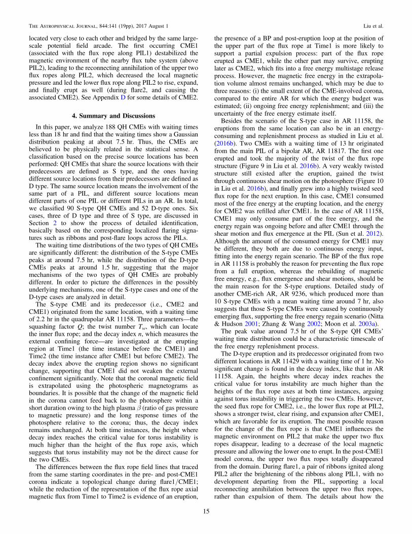
Figure 13. Magnetic features in the vertical cuts, perpendicular to the flux rope at PIL1 in AR 11158, at Time2 (post-CME1 but pre-CME2) and Time3 (post-CME2).Same layout as panels (a)–(f) in Figure 8. 1.25F , given at the headers of panels (a) and (d), are vertical magnetic flux (in units of 1019 Mx) from the strong Tw region(T 1.25w ∣ ∣ ) at each time, respectively. EF, given at the header of panels (b) and (e), are magnetic free energy (in units of 1032 erg) at the two times.

16

The Astrophysical Journal, 844:141 (19pp), 2017 August 1 Liu et al.

1.5hr, could be the characteristic timescale of the growth of

destabilization caused by their predecessors. These kinds of

consecutive CMEs with extremely short waiting times are

sometimes called “twin-CMEs” or “sympathetic-CMEs,”

although they are not necessarily produced from the same

AR (e.g., Balasubramaniam et al. 2011; Schrijver & Title 2011;

Yang et al. 2012; Ding et al. 2013, 2014; Shen et al. 2013). The

source locations of a D-type QH CME and its predecessor

are expected to be located close to each other, or have some

magnetic connection in which one eruption can induce the

other one.Note that there is another slightly lower peak around 9.5hr

in the waiting time distribution of D types, which may be due

to the method of classification, or even a different mechanism

from the one for those with a waiting time around 1.5hr.In conclusion, through the two cases studied in depth, we

propose possible mechanisms for most of the two types of QH

CMEs, i.e., the ones located around the peak of the waiting

time distribution: an S-type QH CME can occur in a recurring

energy release process by free energy regain, while a D-type

QH CME can happen when disturbed by its preceding one. The

different peak values of the waiting time distributions, 7.5hrfor S-type and 1.5 hr for D-type QH CMEs, might be the

characteristic timescales of the two different scenarios. The

classification is only based on the source PILs. An S-type QH

CME may also happen when disturbed by its predecessor,

following a process similar to that for the D-type QH CME, for

example, in a configuration with more than one flux rope

vertically located above the same PIL, like the ones in AR

11429, in which change (reconnection, expulsion, etc.) of the

upper flux ropes caused the eruption of the lower one. More

cases with high spatial and temporal resolution data (e.g., data

from SDO) are worth studying to discover more scenarios.

We thank our anonymous referee for his/her constructivecomments that significantly improved the manuscript. Weacknowledge the use of the data from HMI and AIAinstruments on board Solar Dynamics Observatory (SDO);EIT, MDI, and LASCO instruments on board Solar andHeliospheric Observatory (SOHO); and Transition Region andCoronal Explorer (TRACE). This work is supported by thegrants from NSFC (41574165, 41421063, 41274173,41474151, 41131065), CAS (Key Research Program KZZD-EW-01-4), MOEC (20113402110001), and the fundamentalresearch funds for the central universities.

Appendix AQuality of NLFF Extrapolation

Lorentz force (J B´ , where J is the current density) andthe divergence of the magnetic field ( B · ) should be as smallas possible to meet force-free and divergence-free conditions inthe NLFF coronal fields. We follow Liu et al. (2016b) andWheatland et al. (2000), using two parameters, θ (the anglebetween B and J) and fiá ñ∣ ∣ (fractional flux increase), tomeasure the quality of the model fields:

J B

BJ

sin , 5

J

i

ni

i i

n

i

J

1 1

1

å ås

q s

=´

== =-

⎛

⎝⎜

⎞

⎠⎟

∣ ∣

( )

Bf

n

V

B S

1, 6i

i

ni i

i i1

åá ñ = D

D=

∣ ∣∣ · ∣

·( )

where n is the number of the grid points and ViD and SiD are

the volume and surface area of the ith cell, respectively. Jsgives the average sin q weighted by J. See Table 1 for θ and

fiá ñ∣ ∣ in the aforementioned (and also metioned in the next three

Figure 14. Magnetic features in the vertical cuts, perpendicular to the flux rope at PIL1 in AR 11429, at Time1 (pre-CME1) and Time2 (post-CME1 but pre-CME2).Same layout as in Figure 13.

17

The Astrophysical Journal, 844:141 (19pp), 2017 August 1 Liu et al.

sections) model NLFF fields, which all meet force-free and

divergence-free conditions.

Appendix BChange of Magnetic Parameters during

CME2 in AR 11158

In Section 3.2, the magnetic parameters at the sourcelocation (L1) are studied in pre-CME1 (at Time1) and post-CME1 but pre-CME2 (at Time2) corona. In this appendix, weperform a similar analysis in a plane perpendicular to the fluxrope axis along PIL1 in the post-CME2 corona (2011-02-14T19:46:20 UT, defined as Time3), as shown inFigures 13(d), (e), and (f) (Q, Tw, and B, respectively). Theparameters at Time2 are shown in Figures 13(a)–(c) forcomparison. The triangles mark the peak Tw position, i.e., theposition where the flux rope axis threads the plane. At Time3,the pronounced Q boundary, strong Tw region, and rotationalstructure around the peak Tw point in the in-plane vector fieldsevidence a flux rope. However, the vertical magnetic flux fromthe strong Tw region (T 1.25w ∣ ∣ ) calculated by Equation (3) is

reduced by 77% after CME2 (from 3.10 1019´ Mx at Time2to 0.70 1019´ Mx at Time3, shown at the header ofFigures 13(a) and (d)). The magnetic free energy still shows

a slight increase of 5.5% (from 2.17 1032´ erg at Time2 to2.29 1032´ erg at Time3, as shown at the header ofFigures 13(b) and (e)), which is below the uncertainty.CME2 being confirmed to be correlated to the source locationbased on observation and the decrease of twist of the rope bothevidence that the flux rope is involved in the eruption.However, this information is not enough for distinguishingwhether the flux rope at Time3 is a remnant of the previous fluxrope, which may undergo a partial eruption accompanied bytopology reconfiguration during CME2, or is a newlyemerged/reformed one after CME2. Study of the CME2ʼseruption detail is beyond this paper’s scope.

Appendix CChange of Magnetic Parameters during

CME1 in AR 11429

In Section 3.3, the magnetic parameters at the source locationof CME2 (L2) are studied in pre-CME1 (at Time1) and post-CME1 but pre-CME2 (at Time2) corona to see the possibleinfluence from CME1 to CME2. In this section, we perform asimilar analysis at the source location of CME1 (L1) to see whathappened during CME1. Q, Tw, and B are calculated in a planeperpendicular to the flux rope axis along PIL1 at Time1

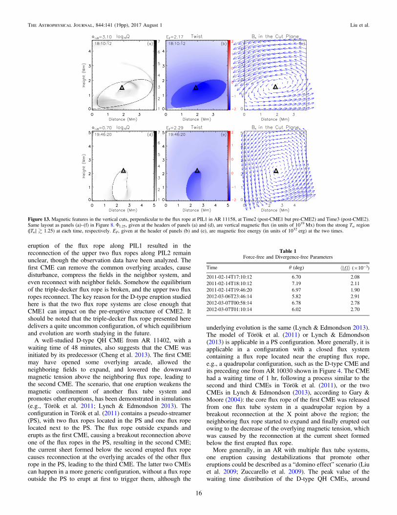
Figure 15. Magnetic features in the vertical cuts, perpendicular to the flux rope at PIL2 in AR 11429, at Time2 (post-CME1 but pre-CME2) and Time3 (post-CME2).Same layout as in Figure 13.

18

The Astrophysical Journal, 844:141 (19pp), 2017 August 1 Liu et al.

(Figures 14(a)–(c)) and Time2 (Figures 14(d)–(f)), respectively.Flux rope is found at PIL1 both before CME1 and after CME1.The vertical magnetic flux from the strong Tw region, with athreshold of 1.25 turns (T 1.25w ∣ ∣ ), shows no significantchange. However, when changing the threshold to 1.6 turns(T 1.6w ∣ ∣ ), the vertical magnetic flux shows a significant

reduction of 47% (from 3.23 1019´ Mx at Time1 to1.70 1019´ Mx at Time2, shown at the header ofFigures 14(a) and (c)). CME1 has been confirmed to be relatedto the source location L1 based on observation, as discussed inSection 2.3; thus, the flux rope should be responsible for theeruption. Its representative axial flux with T 1.6w ∣ ∣ decreased,at the mean time, while the flux with T 1.25w ∣ ∣ almostremained constant. Partial expulsion of the flux rope, accom-panied by replenishment of twist through shear motion orreconnection, can explain the phenomenon.

Appendix DChange of Magnetic Parameters during

CME2 in AR 11429

In this appendix, we perform a similar analysis to that inSection 3.3 in a plane perpendicular to the flux rope axis alongPIL2 in the post-CME2 corona (2012-03-07T01:10:12 UT,defined as Time3), as shown in Figures 15(d), (e), and (f) (Q, Tw,and B, respectively), to see the eruption detail during CME2.The parameters at Time2 are shown in Figures 15(a)–(c) forcomparison. After CME2, there still existed a flux rope alongPIL2, showing a significant topology change compared to that atTime2. The vertical magnetic flux from the strong Tw region(T 1.25w ∣ ∣ ) calculated by Equation (3) decreased by 38% after

CME2 (from 5.66 1019´ Mx at Time2 to 3.51 1019´ Mx atTime3, shown at the header of Figures 15(a) and (d)). Themagnetic free energy also shows a slight decrease of 1.5% (from8.01 1032´ erg at Time2 to 7.89 1032´ erg at Time3, asshown at the header of Figures 15(b) and (e)), which is far belowthe uncertainty. The flux ropes traced by the model method inour cases and two eruptive events in Liu et al. (2016b) all show atwist remnant after the eruption. We come up with two possibleexplanations: it is due to a partial expulsion process or quickreplenishment of twist through emergence/reformation after theeruption. The phenomenon is worth studying in the future.

ORCID

Yuming Wang https://orcid.org/0000-0002-8887-3919Rui Liu https://orcid.org/0000-0003-4618-4979M. Temmer https://orcid.org/0000-0003-4867-7558J. K. Thalmann https://orcid.org/0000-0001-8985-2549Jiajia Liu https://orcid.org/0000-0003-2569-1840Kai Liu https://orcid.org/0000-0003-2573-1531Quanhao Zhang https://orcid.org/0000-0003-0565-3206A. M. Veronig https://orcid.org/0000-0003-2073-002X

References

Akiyama, S., Yashiro, S., & Gopalswamy, N. 2007, AdSpR, 39, 1467Amari, T., Luciani, J. F., Mikic, Z., & Linker, J. 1999, ApJL, 518, L57Balasubramaniam, K. S., Pevtsov, A. A., Cliver, E. W., Martin, S. F., &

Panasenco, O. 2011, ApJ, 743, 202Berger, M. A., & Prior, C. 2006, JPhA, 39, 8321

Brueckner, G. E., Howard, R. a., Koomen, M. J., et al. 1995, SoPh, 162, 357Chatterjee, P., & Fan, Y. 2013, ApJL, 778, L8Chen, C., Wang, Y., Shen, C., et al. 2011, JGR, 116, A12108Cheng, X., Zhang, J., Ding, M. D., et al. 2013, ApJL, 769, L25Chertok, I. M., Grechnev, V. V., Hudson, H. S., & Nitta, N. V. 2004, JGR,

109, 1Chintzoglou, G., Patsourakos, S., & Vourlidas, A. 2015, ApJ, 809, 34DeVore, C. R., & Antiochos, S. K. 2008, ApJ, 680, 740Ding, L., Jiang, Y., Zhao, L., & Li, G. 2013, ApJ, 763, 30Ding, L., Li, G., Dong, L.-H., et al. 2014, JGR, 119, 1463Filippov, B. 2013, ApJ, 773, 10Gary, G. A., & Moore, R. L. 2004, ApJ, 611, 545Gibson, S. E., & Fan, Y. 2006, ApJL, 637, L65Handy, B., Acton, L., Kankelborg, C., et al. 1999, SoPh, 187, 229Hoeksema, J. T., Liu, Y., Hayashi, K., et al. 2014, SoPh, 289, 3483Hood, A. W., & Priest, E. R. 1981, GApFD, 17, 297Jing, J., Tan, C., Yuan, Y., et al. 2010, ApJ, 713, 440Kaiser, M. L., Kucera, T. a., Davila, J. M., et al. 2008, SSRv, 136, 5Kienreich, I. W., Veronig, A. M., Muhr, N., et al. 2011, ApJL, 727, L43Kliem, B., & Török, T. 2006, PhRvL, 96, 255002Kliem, B., Török, T., Titov, V. S., et al. 2014, ApJ, 792, 107Lemen, J. R., Title, A. M., Akin, D. J., et al. 2012, SoPh, 275, 17Li, T., & Zhang, J. 2013, ApJL, 778, L29Liu, C., Lee, J., Karlický, M., et al. 2009, ApJ, 703, 757Liu, L., Wang, Y., Wang, J., et al. 2016a, ApJ, 826, 119Liu, R., Kliem, B., Titov, V. S., et al. 2016b, ApJ, 818, 148Liu, R., Kliem, B., Török, T., et al. 2012, ApJ, 756, 59Liu, Y. 2008, ApJL, 679, L151Lynch, B. J., & Edmondson, J. K. 2013, ApJ, 764, 87MacTaggart, D., & Hood, A. W. 2009, A&A, 508, 445Moon, Y.-J., Chae, J., Wang, H., & Park, Y. 2003a, AdSpR, 32, 1953Moon, Y.-J., Choe, G. S., Wang, H., & Park, Y. D. 2003b, ApJ, 588, 1176Nitta, N. V., & Hudson, H. S. 2001, GeoRL, 28, 3801Pesnell, W. D., Thompson, B. J., & Chamberlin, P. C. 2012, SoPh, 275, 3Schmieder, B. 2006, JApA, 27, 139Schou, J., Scherrer, P. H., Bush, R. I., et al. 2012, SoPh, 275, 229Schrijver, C. J. 2009, AdSpR, 43, 739Schrijver, C. J., & Title, A. M. 2011, JGR, 116, A04108Shen, C., Li, G., Kong, X., et al. 2013, ApJ, 763, 114Soenen, A., Zuccarello, F. P., Jacobs, C., et al. 2009, A&A, 501, 1123Su, J. T., Jing, J., Wang, S., Wiegelmann, T., & Wang, H. M. 2014, ApJ,

788, 150Su, Y., van Ballegooijen, A., McCauley, P., et al. 2015, ApJ, 807, 144Subramanian, P., & Dere, K. P. 2001, ApJ, 561, 372Sun, X., Bobra, M. G., Hoeksema, J. T., et al. 2015, ApJL, 804, L28Sun, X., Hoeksema, J. T., Liu, Y., Chen, Q., & Hayashi, K. 2012, ApJ,

757, 149Thalmann, J. K., Su, Y., Temmer, M., & Veronig, A. M. 2015, ApJL,

801, L23Thalmann, J. K., Wiegelmann, T., & Raouafi, N.-E. 2008, A&A, 488, L71Tian, L., Liu, Y., & Wang, J. 2002, SoPh, 209, 361Titov, V. S. 2007, ApJ, 660, 863Titov, V. S., & Démoulin, P. 1999, A&A, 351, 707Titov, V. S., Hornig, G., & Démoulin, P. 2002, JGR, 107, 1164Titov, V. S., Priest, E. R., & Démoulin, P. 1993, A&A, 276, 564Török, T., & Kliem, B. 2003, A&A, 406, 1043Török, T., & Kliem, B. 2005, ApJL, 630, L97Török, T., Panasenco, O., Titov, V. S., et al. 2011, ApJL, 739, L63Wang, Y., Chen, C., Gui, B., et al. 2011, JGR, 116, A04104Wang, Y., Liu, L., Shen, C., et al. 2013, ApJL, 763, L43Wang, Y., & Zhang, J. 2007, ApJ, 665, 1428Webb, D. F., & Howard, T. A. 2012, LRSP, 9, 3Wheatland, M. S., Sturrock, P. a., & Roumeliotis, G. 2000, ApJ, 540, 1150Wiegelmann, T. 2004, SoPh, 219, 87Wiegelmann, T., Thalmann, J. K., Inhester, B., et al. 2012, SoPh, 281, 37Yang, J., Jiang, Y., Zheng, R., et al. 2012, ApJ, 745, 9Yashiro, S. 2004, JGR, 109, A07105Yashiro, S., Michalek, G., Akiyama, S., Gopalswamy, N., & Howard, R. A.

2008, ApJ, 673, 1174Zhang, J., & Wang, J. 2002, ApJL, 566, L117Zhou, G., Wang, J., & Cao, Z. 2003, A&A, 397, 1057Zuccarello, F., Romano, P., Farnik, F., et al. 2009, A&A, 493, 629Zuccarello, F. P., Aulanier, G., & Gilchrist, S. A. 2016, ApJL, 821, L23

19

The Astrophysical Journal, 844:141 (19pp), 2017 August 1 Liu et al.