the clarion cognitive architecture: a tutorial part 2 – the action- centered subsystem nick...

The CLARION Cognitive The CLARION Cognitive Architecture: A TutorialArchitecture: A Tutorial

Part 2 – The Action-Part 2 – The Action-Centered SubsystemCentered Subsystem

Nick Wilson, Michael Lynch, Ron Sun, Sébastien HélieCognitive Science, Rensselaer Polytechnic Institute

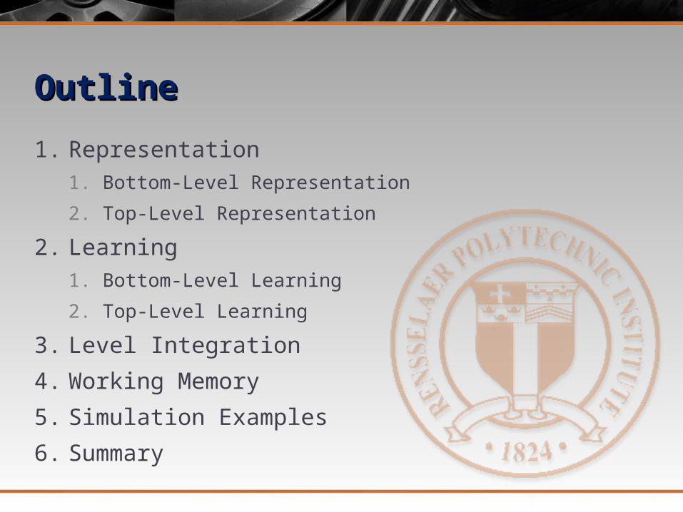
OutlineOutline

1. Representation1. Bottom-Level Representation

2. Top-Level Representation

2. Learning1. Bottom-Level Learning

2. Top-Level Learning

3. Level Integration

4. Working Memory

5. Simulation Examples

6. Summary

RepresentationRepresentation

1.1. RepresentationRepresentation1. Bottom-Level Representation



2. Top-Level Rule Learning


4. Working Memory


6. Summary


Top-level

Bottom-level

Action-centeredExplicit

Representation

Action-centeredExplicit

Representation

Action-centeredImplicit

Representation

Action-centeredImplicit

Representation

Non-action-centeredExplicit

Representation

Non-action-centeredExplicit

Representation

Non-action-centeredImplicit

Representation

Non-action-centeredImplicit

Representation

ACS NACS


Action Decision making process:1. Observe the current state.

2. Compute in the bottom level the “value” of each of the possible actions in the current state. E.g., stochastically choose one action.

3. Find out all the possible actions at the top level, based on the current state information and the existing rules in place at the top level. E.g., stochastically choose one action.

4. Choose an appropriate action by stochastically selecting or combining the outcomes of the top level and the bottom level.

5. Perform the selected action and observe the next state along with any feedback (i.e. reward/reinforcement).

6. Update the bottom level in accordance with, e.g., reinforcement learning (e.g., Q-learning, implemented with a backpropogation network).

7. Update the top level using an appropriate learning algorithm (e.g., for constructing, refining, or deleting explicit rules).

8. Go back to step 1.


1. Representation

1.1. Bottom-Level RepresentationBottom-Level Representation2. Top-Level Representation




4. Working Memory


6. Summary


Bottom Level Implicit knowledge is:

Less accessible

Reactive (as opposed to, e.g., explicit planning; fast decision making)

Inaccessible nature of implicit (tacit) knowledge (Reber, 1989; Sun, 2002) may be captured by distributed representations

a theoretical interpretation

E.g., Backpropagation Neural Networks:

Representational units are capable of accomplishing tasks but are generally not individually meaningful --- renders distributed representation less accessible.


At the bottom level, Implicit Decision Networks (IDNs): implemented with Backpropagation networks

The current state is represented as dimension-value pairs: (dim1, val1) (dim2, val2) … (dimn, valn)

Each pair corresponds to one input node of the network

Three types of inputs:

Sensory Input (visual, auditory, …., etc.)

Working Memory Items

Goal Structure Item


Actions are represented as nodes on the output layer. Three types of actions:

o Working Memory Actions

o Goal Actions

o External Actions

Each action consists of one or more action dimensions in the form:

(dim1, val1) (dim2, val2) … (dimn, valn)


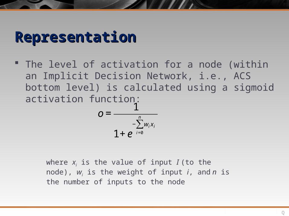
The level of activation for a node (within an Implicit Decision Network, i.e., ACS bottom level) is calculated using a sigmoid activation function:

€

o =1

1+ e− wi xii=0

n

∑

where xi is the value of input I (to the node), wi is the weight of input i, and n is the number of inputs to the node

Q


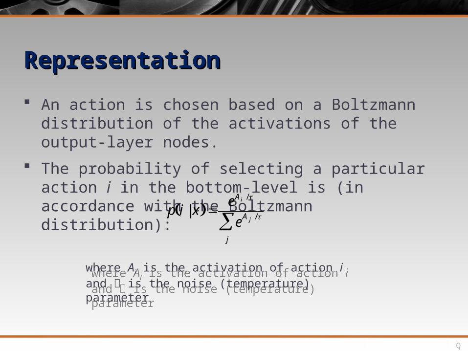
An action is chosen based on a Boltzmann distribution of the activations of the output-layer nodes.

The probability of selecting a particular action i in the bottom-level is (in accordance with the Boltzmann distribution):

p i | x eA i /

eA j /

j

where Ai is the activation of action i and is the noise (temperature) parameter

where Ai is the activation of action i and is the noise (temperature) parameter

Q


WM ActionNetwork

WM ActionNetwork

External Action Network

External Action Network

GS ActionNetwork

GS ActionNetwork

GoalStructure

GoalStructure

WorkingMemory

WorkingMemory

WM action

External action

WM content

GS action

Current goalSensory input


Questions?



2.2. Top-Level RepresentationTop-Level Representation




4. Working Memory


6. Summary

RepresentationRepresentation Top Level

Explicit Rules:o more accessible

o “rationally”, “consciously” deduced actions

o slower than implicit processes, but also perhaps more precise

o “Condition Action” pairs:

Condition Chunk

Action Chunk

Rules in the top level come from several sources (more on this later):o Extracted and Refined Rules (RER rules)

o Independently Learned Rules (IRL rules)

o Fixed Rules (FR rules)


Chunks are collections of dimension/value pairs that represent either conditions or actions in the top level.

Chunk-idi: (dimi1, vali1) (dimi2, vali2)…(dimini, valini

)

e.g., table-1: (size, large) (color, white) (number-of-legs, 4)

Each chunk (as a whole) is represented by a node in the top level

Each dimension/value pair is represented by a node in the bottom level.

Dual representation: Localist versus distributed representation


A top-level rule contains one condition and one action (possibly with multiple dimensions)

Action is associated with these factors: Base-Level Activation (BLA)

Recency-based value (e.g., used for determining RTs)

Utility (U)Measures the usefulness of a rule based on the cost and benefit of the rule (e.g., used for selecting rules)

other numerical measures


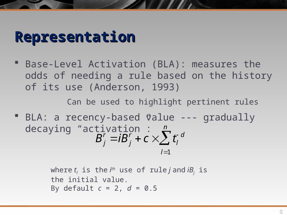
Base-Level Activation (BLA): measures the odds of needing a rule based on the history of its use (Anderson, 1993) Can be used to highlight pertinent rules

BLA: a recency-based value --- gradually decaying “activation”:

B jr iB j

r c tl d

l1

n

where tl is the ith use of rule j and iBj is the initial value. By default c = 2, d = 0.5

Q


Rule selection at the top level:

based on a Boltzmann distribution of the utility of the rule (which may be set to a constant if not needed)

Utility may be calculated using the following equation:

jjrj costbenefitU

where is a scaling factor balancing measurements of benefits and costs

Q

Representation*Representation*

Benefit:

Cost:

benefit j c7 PM( j)

c8 PM( j) NM( j)

€

cost j =execution time of rule j

average execution time of rules

where PM(j) = number of positive rule matches and NM(j) = number of negative rule matches. By default c7 = 1, c8 = 2

where values need to be estimated (domain-specific)

Q


Questions?

LearningLearning



2.2. LearningLearning1. Bottom-Level Learning



4. Working Memory


6. Summary

LearningLearning Bottom-Level Learning

Uses Backpropagation to perform error correction within the bottom level (IDN’s)

Three learning methods:o Standard Backpropagation (supervised learning)

o Q-Learning (reinforcement learning)

o Simplified Q-Learning

Top-Level Rule Learning Three methods:

o Bottom-up rule extraction and refinement (RER)

o Independent Rule Learning (IRL)

o Fixed Rule (FR)

LearningLearning



2. Learning

1.1. Bottom-Level Implicit LearningBottom-Level Implicit Learning2. Top-Level Rule Learning


4. Working Memory


6. Summary

LearningLearning

Standard Backpropagation (for three-layer network) Calculate error in the output layer using:

Output weights are updated as follows:

erri target(x,ai) Q(x,ai)

where target(x,ai) is the target output for node i and Q(x,ai) is the actual output of node i

w ji x ji j

j errjo j (1 o j )

where xji is the ith input of output unit j and oj is the output of unit j

Q

Learning*Learning*

Standard Backpropagation (cont.) Weights are updated in the hidden layer by:

kkjkjjj

jijji

woo

xw

)1(

where xji is the ith input to hidden unit j, is the learning rate, oj is the output of hidden unit j, and k denotes all of the units downstream (in the output layer) of hidden unit j

Q

LearningLearning

Q-Learning A reinforcement learning method (as opposed to supervised learning)

Updating based on the temporal difference in evaluating the current state and the current action chosen

Uses backpropagation, except error is calculated in the output layer using:

erri 0 otherwisere(y ) Q(x,a i ) if a ia

where r + e(y) estimates the (discounted) total reinforcement to be received from the current point on.

Q

LearningLearning

Q-Learning (cont.) Q(x,a) approaches:

e(y) is calculated using:

Q

Q(x,a) a i :i1,2,3,... max ( iri

i0

)

where is a discount factor, ai is an action that can be performed at step i, and ri is the reinforcement received at step i

)),((max)( byQye b

where y is the new state resulting from action a in state x

LearningLearning

Simplified Q-Learning Basic form (atemporal) reinforcement learning

Temporal credit assignment is not involved

Most useful when immediate feedback is available and sufficient

Error is calculated in the output layer using:

erri 0 otherwiser Q(x,a i ) if a ia

Q

LearningLearning

Context for Reinforcement Learning --- Two loops:

Sensory Input → Action (e.g., by implicit reactive routines within the ACS, formed by, e.g., reinforcement learning)

Sensory Input → MS → MCS → Reinforcement signal (to be used in the ACS for reinforcement learning)

In addition to other loops

LearningLearning

Questions?

LearningLearning




2.2. Top-Level LearningTop-Level Learning


4. Working Memory


6. Summary

LearningLearning

Top Level Learning Bottom-up rule extraction and refinement (RER)

“Condition → Action” pairs are extracted from the bottom level and refined (generalized, specialized, or deleted) as necessary

Independent rule learning (IRL)

Rules of various forms are independently generated (either randomly or in a domain-specific order) and then refined or deleted as needed

Fixed Rules

Rules are obtained from prior experiences, or provided from external sources

LearningLearning

Rule extraction and refinement (RER) Basic idea of the algorithm:

If an action decided by the bottom level is successful (according to a criterion), then a rule is constructed and added to the top level

In subsequent interactions with the world, the rule is refined by considering the outcome of applying the rule:

• If the outcome is successful, the condition of the rule may be generalized to make it more universal

• If the outcome is not successful, then the condition of the rule should be made more specific

LearningLearning

Rule extraction Check the current criterion for rule extraction

If the result is successful according to the current rule extraction criterion, and there is no rule matching the current state and action, then perform extraction of a new rule

• “Condition → Action”

• Add the extracted rule to the action rule store at the top level

LearningLearning

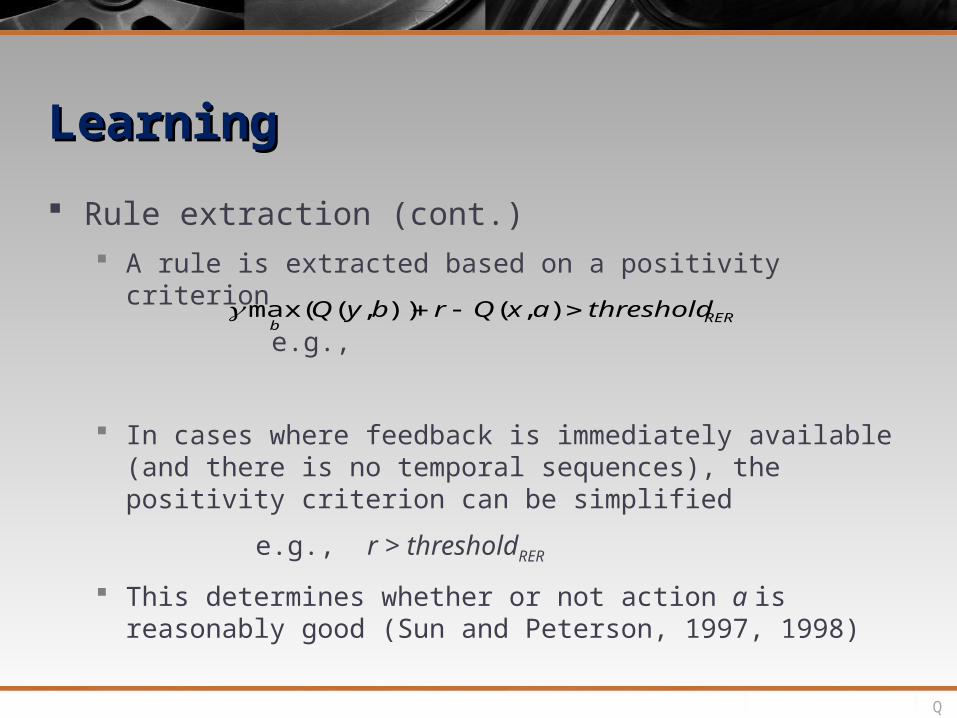
Rule extraction (cont.) A rule is extracted based on a positivity criterion

e.g.,

In cases where feedback is immediately available (and there is no temporal sequences), the positivity criterion can be simplified

e.g., r > thresholdRER

This determines whether or not action a is reasonably good (Sun and Peterson, 1997, 1998)

RERb

axQrbyQ threshold ),()),((max

Q

LearningLearning

Refinement Extracted rules (or Independently learned rules) have rule

statistics that guide rule refinement• Positive Match PM:=PM+1 when the positivity criterion is met

• Negative Match NM:=NM+1 when the positivity criterion is not met

• At the end of each episode (e.g., a game, an action sequence, etc.), PM and NM are discounted by multiplying them by .9

LearningLearning

Refinement (cont.) Based on PM and NM, an information gain measure (IG) may be

calculated:

essentially compares the percentages of positive matches under different conditions: A vs. B

If A can improve the percentage to a certain degree over B, then A is considered better than B

IG(A,B) log2(PMa (A) c1

PMa (A) NMa (A) c2

) log2(PMa (B) c1

PMa (A) NMa (A) c2

)

where A and B are two different rule conditions that lead to the same action a, c1 and c2 are constants (1 and 2 respectively by default)

Q

LearningLearning

Generalization Check the current criterion for Generalization

• If the result is successful according to the current generalization criterion, then generalize the rules matching the current state and action

• Remove these rules from the rule store

• Add the generalized versions of these rules to the rule store (at the top level)

LearningLearning

Generalization (cont.) A rule can be generalized using the information gain measure:

• If IG(C, all) > threshold1 and maxc’ IG(C’, C) 0 , then set

C” = argmaxC’ (IG (C’, C))

as the new (generalized) condition of the rule

• Reset all the rule statistics

where C is the current condition of the rule, all is the match-all rule, and C’ is a modified condition such that C’ = “C plus one value”

LearningLearning

Specialization Check the current criterion for Specialization

• If the result is unsuccessful according to the current specialization criterion then revise all the rules matching the current state and action

• Remove the rules from the rule store

• Add the revised (specialized) rules into the rule store (at the top level)

LearningLearning

Specialization (cont.) A rule can be specialized using the information gain measure:

• If IG(C,all) < threshold2 and maxC’IG(C’,C) > 0, then set

C”=argmaxC’ (IG (C’, C))

as the new (specialized) condition of the rule

where C is the current state condition of the rule, all is the match-all rule, C’ is a modified condition such that C’ = “C minus one value”

• If any dimension in C has no value left after specialization then the rule is deleted

• Reset all the rule statistics

LearningLearning

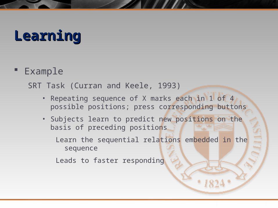
ExampleSRT Task (Curran and Keele, 1993)

• Repeating sequence of X marks each in 1 of 4 possible positions; press corresponding buttons

• Subjects learn to predict new positions on the basis of preceding positions

Learn the sequential relations embedded in the sequence

Leads to faster responding

LearningLearning

Example (cont.) Learning (by iterative weight updating) in the bottom level promotes

implicit knowledge formation (embedded in weights)

Resulting weights specify a function relating previous positions (input) to current position (output)

Acquired sequential knowledge at the bottom level can lead to the extraction of explicit knowledge at the top level

LearningLearning

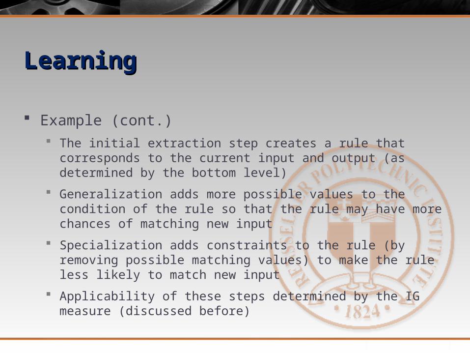
Example (cont.) The initial extraction step creates a rule that corresponds to the current

input and output (as determined by the bottom level)

Generalization adds more possible values to the condition of the rule so that the rule may have more chances of matching new input

Specialization adds constraints to the rule (by removing possible matching values) to make the rule less likely to match new input

Applicability of these steps determined by the IG measure (discussed before)

LearningLearning

Example (cont.) Suppose sequence is:

1 2 3 2 3 4

Initially extracted rule may be:

1 2 3 2 3 --> 4

Generalization may lead to a simplified rule:

* 2 3 2 3 --> 4 (where * stands for “don’t care”)

* 2 * 2 3 --> 4

and so on

Continued generalizations and specializations are likely to happen, as determined by the IG measure (which is in turn determined by the performance of the rule)

Incorrect generalization may occur (e.g., 2 3 4), which may then be revised

Learning (RER)Learning (RER)

Questions?

LearningLearning

Independent Rule Learning (IRL) A variation of rule extraction and refinement

In which, the bottom level is not used for initial rule extraction.

Rules are generated either randomly or through a domain-specific order

Then these rules are tested through experience using the IG measure

If the rule IG measure is below a threshold, then the rule is refined or deleted.

LearningLearning

Independent Rule Learning (cont.) Positivity criterion can be based on information from the bottom level

(similar to RER):

e.g.,

Positivity criterion can also be based on information from external sources (such as immediate feedback/reinforcement)

IRLb

thresholdaxQrbyQ ),()),((max

Q

LearningLearning

Independent Rule Learning (cont.) One possible information gain measure for IRL rule testing is:

If IG(C, random) < threshold3 then delete the rule

This is equivalent to:

Specialization/generalization are also possible (similar to RER; assuming a match-all condition to begin with).

If IG(C) log2(PMa (C) c5

PM(C) NM(C) c6

) threshold4 then delete rule C

Q

LearningLearning

Fixed Rules (FR) Externally given or acquired from prior experiences (or by pre-

endowment?)

Enables top-down learning (assimilation)

Rules in the top level may guide implicit learning in the bottom level.

Can represent more than just propositional structures

More complex interaction, and more complex action sequences between conditions and actions, akin to:

• Schemas (Arbib, 1980; Dretcher, 1989)

• Abstract behaviors (Mataric, 2001)

Q

Learning (IRL and FR)Learning (IRL and FR)

Questions?

Level IntegrationLevel Integration





3.3. Level IntegrationLevel Integration4. Working Memory


6. Summary


Several level integration methods: Stochastic Selection Combination

Bottom-up Rectification

Top-down Guidance

Assumes one bottom-level network and one top-level rule group

Details on coordinating multiple bottom-level networks and top-level rule groups can be found in the technical descriptions (Sun, 2003)

Q


Stochastic Selection

At each step, the probability of using any given rule set is:PRER = probability of using RER rule set

PIRL = probability of using IRL rule set

PFR = probability of using FR rule set

The probability of using the bottom level is:PBL = 1 - PRER - PIRL - PFR

Q


Selection probabilities may be: Fixed (pre-set/constant; e.g. set by the Meta-Cognitive Subsystem)

Variable (see later)

Deterministic selection of either the top level or the bottom level is a special case of stochastic selection --- probability=1/0 Selection probabilities in this case may be chosen by the Meta-Cognitive

Subsystem (discussed later)


Variable selection probabilities: may be calculated using “probability matching”, as follows:

PBL BL srBL

PRER RER srRER

PIRL IRL srIRL

PFR FR srFR

where sr stands for success rate, is a weighting parameter, and = BL x srBL+ RER x srRER + IRL x srIRL + FR x srFR

Q


Combination Combining activation from the top level with Q-values in the bottom

level, in some way

Top-down guidance vs. bottom-up rectification

Then selecting an action based on the combined values using a Boltzmann distribution

Positive conclusions reached in the top level can add to action recommendations in the bottom level

Negative conclusions reached in the top level can veto actions in the bottom level

H


Bottom-up Rectification: Bottom-level outcome is sent to the top level

The top level rectifies and utilizes outcomes from the bottom level with the knowledge in the top level

(One possibility: weighted sum combination)

Likely to happen in reasoning situations, where final outcomes are explicit (Nisbett and Wilson 1977)

H


Top-down Guidance: Top-level outcome is sent down to the bottom level

The bottom level utilizes the outcome of the top level, along with its own knowledge, in making action decisions

(One possibility: weighted sum combination)

Most likely happens in skilled learning and skilled performance

H

OverviewOverview

Action Decision making process:1. Observe the current state.

2. Compute in the bottom level the “value” of each of the possible actions in the current state. E.g., stochastically choose one action.

3. Find out all the possible actions at the top level, based on the current state information and the existing rules in place at the top level. E.g., stochastically choose one action.

4. Choose an appropriate action by stochastically selecting or combining the outcomes of the top level and the bottom level.

5. Perform the selected action and observe the next state along with any feedback (i.e. reward/reinforcement).

6. Update the bottom level in accordance with, e.g., reinforcement learning (e.g., Q-learning, implemented with a backpropagation network).

7. Update the top level using an appropriate learning algorithm (e.g., for constructing, refining, and deleting explicit rules).

8. Go back to step 1.

Questions?


Working MemoryWorking Memory






4.4. Working MemoryWorking Memory5. Simulation Examples

6. Summary

H

Working MemoryWorking Memory For storing information on a temporary basis

Facilitating subsequent action decision-making and/or reasoning

Working memory involves: Action-directed (“deliberate”) encoding of information

(As opposed to automatic encoding)

Gradual fading of information Action-directed re-encoding (“refreshing”) of information Limited storage capacity Multiple stores

(cf. Baddelay, 1995)

H


May be divided into multiple sensory related sections: Visuospatial information

Auditory/verbal information

Other types of information

Each section consists of a certain number of slots Each can hold the content of a chunk

Capacity is limited

H


Working memory actions may: Add an item into working memory

Set i: the content of a chunk is stored in working memory slot i

Set {i}: the content of multiple chunks are stored in multiple slots in working memory

Remove an item from working memoryReset i: the content of the ith working memory slot is removed

Reset-all-WM: removes all items from working memory

Do-nothing

Working Memory actions can be performed by either or both levels

H


Base-level activation (BLA) for WM: Determines how long past information should be kept around (when

there is no reset action)

Recency-based:

Biw iBi

w c tl d

l1

n

where i indicates an item in working memory, l indicates the lth setting of that item, tl is the time since the lth setting, and iB is the initial value of B (c and d are constants)

H


If the base-level activation of working memory item i is above a threshold:

then the working memory item i is used as input to the bottom level and the top level

Biw thresholdWM

H

Working Memory and NACSWorking Memory and NACS

Working memory may be used to transmit information between the Action-Centered (ACS) and Non-Action-Centered (NACS) subsystems (discussed later)

Working memory is minimally necessary for storing information from the non-action-centered subsystem, because

Must be able to retrieve and hold conclusions from reasoning so it can be used for action-decision making.

Must be able to extract additional declarative information about the current state and action (including related past episodes, which is also stored in the NACS)

H


Questions?

H

Simulation ExamplesSimulation Examples






4. Working Memory

5.5. Simulation ExamplesSimulation Examples6. Summary


Serial reaction time task (Curran and Keele, 1993) A sequence of X marks

Two phases:

• Single task learning

• Dual task transfer

Three groups of subjects:

• Less aware

• More aware

• Intentional

H


3 (intentional vs. more aware vs. less aware) X 2 (sequential vs. random) ANOVA: significant difference across groups during the STL phase No difference across groups during the DTT phase

H


Model Setup Simplified Q-backpropagation learning in the bottom level 7x6 input units (both primary and secondary tasks) and 5 output units RER rule learning Three groups:

• Less aware - use higher rule learning thresholds

• More aware - use lower rule learning thresholds

• Intentional - code given knowledge in the top level

Linear transformation: Rti = a ⨯ ei + b ANOVA confirmed the data pattern

H


Plot from Cleeremans (1993) SimulationPlot from Cleeremans (1993) Simulation

Human data from Curran & KeeleHuman data from Curran & Keele

Plot from CLARION SimulationPlot from CLARION Simulation HH


Letter counting task (Rabinowitz and Goldberg, 1995) Experiment 1

• letter1 + number = letter2

• The consistent group:

• 36 blocks of training (the same 12 addition problems in each)

• The varied group:

• 6 blocks of training (the same 72 addition problems in each)

• Transfer

• 12 new addition problems (repeated 3 times)


Letter counting task (cont.) Experiment 2

• Same training

• Transfer:

• 12 subtraction problems (repeated 3 times)

• letter1 - number = letter2 (reverse of addition problems)

Simulation Examples

Experiment 1 Experiment 2


Model Setup Simplified Q-backpropagation learning in the bottom level ACS (IDNs)

35 input units, 26 output units, and 30 hidden units

Fixed Rules

• If goal=addition-counting, start-letter=x, number=y, then starting with x, repeat y times counting up

• If goal=subtraction-counting, start-letter=x, number=y, then starting with x, repeat y times counting down

Q


Model Setup (cont.) Rule utility (for rule selection) and rule base-level activation (for

response time)

Response Time:

€

DTTL = y × tcounting + c ×1

BLA(rule)

DTBL = constant

Q

Simulation ExamplesSimulation Examples Experiment 1: CLARION vs. ACT-R

Rabinowitz and Goldberg Experimental ResultsRabinowitz and Goldberg Experimental Results

CLARION Simulation ResultsCLARION Simulation Results ACT-R Simulation ResultsACT-R Simulation Results

Simulation ExamplesSimulation Examples Experiment 2: CLARION vs. ACT-R (cont.)

CLARION Simulation ResultsCLARION Simulation Results ACT-R Simulation ResultsACT-R Simulation Results

Rabinowitz and Goldberg Experimental ResultsRabinowitz and Goldberg Experimental Results


Learning curve of Rabinowitz and Goldberg (1995) Learning curve during the simulation


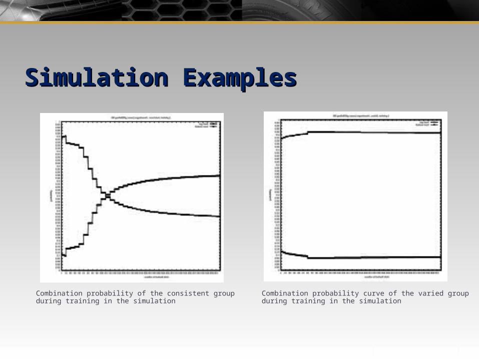
Combination probability of the consistent group during training in the simulation

Combination probability curve of the varied group during training in the simulation


Questions?


Minefield navigation task (Sun et al 2001)

H


Four training conditions: Standard training condition

Verbalization condition

Dual-task condition

Transfer conditions

H


Model Setup The effect of the dual task is captured by reduced top-level activities

(through raised rule learning thresholds)

The effect of regular verbalization stems from heightened rule learning activities (through lowered rule learning thresholds)

The model starts with no more a priori knowledge about the task than a typical human subject

10 human subjects were compared to 10 model subjects in each experiment

H


The effect of the dual task condition on learning:

2 (human vs. model) X 2 (single vs. dual task) ANOVA indicated a significant main effect for single vs. dual task (p < .01), but no interaction between groups and task types

H


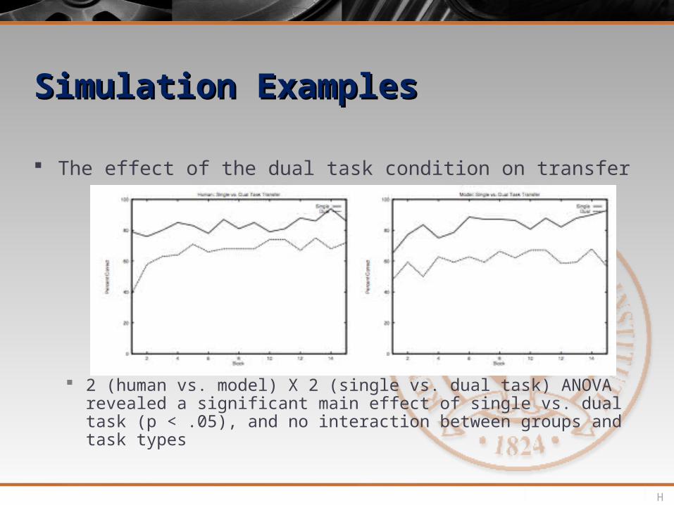
The effect of the dual task condition on transfer

2 (human vs. model) X 2 (single vs. dual task) ANOVA revealed a significant main effect of single vs. dual task (p < .05), and no interaction between groups and task types

H


The effect of verbalization

4 (days) X 2 (human vs. model) X 2 (verbalization vs. Standard) ANOVA indicated that both human and model subjects exhibited a significant increase in performance due to verbalization (p < .01), but that the difference associated with verbalization for the two groups was not significant

H


Academic science task (Naveh and Sun, 2006) Number of authors contributing a certain number of articles follows

an inverse power law: a Zipf distribution (Lotka, 1926) Simon (1957): a simple stochastic process for approximating Lotka’s

law The probability that a paper will be published by an author who has

published i articles is a/ik

Gilbert (1997) simulated Lotka’s law Assumed that authors were non-cognitive and interchangeable; it neglected

a host of cognitive phenomena that characterized scientific inquiry (e.g., learning, creativity, evolution of field expertise, etc.)

H


Setup for simulating academic publishing data:o Multiple agents: with limited academic life spans (in part, depending on

productivity)

o Each paper: based on combining past ideas (past papers), with local optimization

o Action sequences in generating papers: decided based on implicit and explicit knowledge, with learning from experiences

o Evaluated based on a set of criteria (i.e., refereed)


H

Simulation Examples*Simulation Examples*

The CLARION simulation data for the two journals matched the real-world data well

The CLARION simulation data for the two journals could be fit to the power curve f(i) = a/ik

Q


The number of papers per author reflected cognitive processes of authors, as opposed to being based on auxiliary assumptions

Emergent, not a result of direct attempts to match the human data

More distance between mechanisms and outcomes, to come up with deeper explanations

H


Varying cognitive parameters: Most prolific under a moderately high temperature setting:

Serendipity in scientific discovery!

H

Simulation ExamplesSimulation Examples Varying cognitive parameters:

Generate different communities producing different numbers of papers, by varying cognitive parameters

Power curves are obtained under different cognitive parameter settings

H


Varying cognitive parameters: Cognitive-social invariance

General applicability and validity of the model

Generate new theories and hypotheses

Reduce the need for costly (or impossible) human experiments

H


Questions?

SummarySummary






4. Working Memory


6. Summary

SummarySummary

ACS Bottom level: implicit representation Implemented by

e.g., backpropagation networks

Bottom-level learning modes:

• Standard backpropagation learning

• Q-learning

• Simplified Q-learning

SummarySummary

ACS Top level: explicit representation Rules: “condition action” pairs

Types of top-level rules:

• Rule extraction and refinement (RER)

• Independent Rule Learning (IRL)

• Fixed Rules (FR)

SummarySummary

Level Integration Stochastic Selection

• Level is chosen probabilistically

Combination• Bottom-up rectification

• Bottom-level outcome rectified at the top level

• Top-down guidance

• Top-level outcome assists action decision-making at the bottom level

o Both may boil down to weighted-sum

SummarySummary

Working Memory Involves:

• Action-directed encoding of information (as opposed to automatic encoding)

• Gradual fading of information (using BLA)

• Action-directed re-encoding (“refreshing”) of information

• Limited storage capacity

Working memory is also used to transmit information between the action-centered and non-action-centered subsystems.

H

SummarySummary

Thank You

Questions?

the clarion cognitive architecture: a tutorial part 2 – the action- centered subsystem nick...

Documents

level action

representation actions

toplevel representation

implicit representation

explicit representation

representation action

level integration

level implicit knowledge