the colonial origins of comparative development: … critique focuses in particular on three issues....

2007

-9Sw

iss

Nati

onal

Ban

k W

orki

ng P

aper

sThe Colonial Origins Of Comparative Development: Comment.A Solution to the Settler Mortality Debate Raphael Auer

The views expressed in this paper are those of the author(s) and do not necessarilyrepresent those of the Swiss National Bank. Working Papers describe research in progress.Their aim is to elicit comments and to further debate.

ISSN 1660-7716

© 2007 by Swiss National Bank, Börsenstrasse 15, P.O. Box, CH-8022 Zurich

The Colonial Origins Of Comparative Development: Comment.

A Solution to the Settler Mortality Debate

Raphael Auer�

Swiss National Bank

28 February 2007

PRELIMINARY AND INCOMPLETE DO NOT CITE OR DISTRIBUTE

Abstract

I address David Albouy’s (2006) critique of the data constructed by Daron Acemoglu, Si-

mon Johnson and James Robinson (2001). The contribution of this paper is to instrument for

settler mortality rates that are collected from historical sources — and that may be measured

with error — with a geographic model of the determinants of disease. I first establish that

my instruments are significant predictors of mortality and are otherwise excludable to institu-

tions. Among other things, the excludability is established by a falsification exercise, in which

I document that the geographic potential for mortality strongly a ected institutions in former

colonies, yet it had no e ect on institutions in the rest of the world. This di erential e ect

settler mortality had on development can only be rationalized by the early institution building

hypothesis that Acemoglu et al. argue for. I next repeat the analysis of Acemoglu et al. in-

strumenting for the historical mortality rate with its geographic projection. The instrumented

mortality rate is a highly significant predictor of institutional quality. Moreover, this result is

true when instrumenting for either the original data or the revised mortality series of Albouy.

This result is also true when accounting for the population that the historical data was sampled

from. Turning to the instrumental variable estimations, I show that also the relation between

institutions and income is highly significant and that the associated importance of institutions

for international income di erences is substantial. Again this finding is true when using either

of the two historical series and also when accounting for the population that the historical

data was sampled from. I thus conclude that the empirical results presented in Acemoglu et

al. indeed reflect their early institution building hypothesis rather than measurement error.

�Contact: Email: [email protected], I thank Daron Acemoglu, Josh Angrist, Andrei Shleifer and

especially Gerard Padro-I-Miguel for helpful discussions. I thank Domagoj Arapovic for excellent research

assistance.

1

1 Introduction

With their seminal work on the effect colonization policies had on comparative development,

Daron Acemoglu, Simon Johnson and James Robinson (2001) develop a strong case for the im-

portance of property rights institutions as the ultimate cause of economic prosperity. Building on

earlier work of Knack and Keefer (1995), Mauro (1995), La Porta et al. (1998), and Hall and Jones

(1999), the authors argue that early settlement policies were influenced by the mortality rates

potential settlers faced in the colonies. They show that the number of Europeans that settled in

a colony influenced the colonization policies adopted by imperialist nations, with very different

associated institutional outcomes.

The authors’ most important contribution is to construct an instrumental variable — the mor-

tality rate of European settlers in former colonies — that is strongly related to institutional quality,

yet has no direct impact on income differences. Using their measure of the settler mortality rate

in former colonies, the authors establish that institutions are the main determinant of economic

prosperity.

Collecting the mortality rates of settlers during colonization is a difficult task, and Acemoglu

et al. rely on several sources to construct their series of mortality rates for 64 countries. Their

most important source is Curtin (1989), who collected mortality rates from soldiers stationed in

former colonies. However, this measure is not available for many nations and the authors thus

rely on mortality rates of bishops from Guiterrez (1986) and on mortality rates of laborers from

Curtin (1998).

When working with data that originated up to 300 years ago and is collected from various

sources, it is inevitable that coverage is incomplete and that the data is measured with some

error. David Albouy’s (2006)1 comment on the quality of this data, however, does not address

the mere fact that there may be additional noise in the data. Rather, he asserts that the settler

mortality data suffers from systematic shortcomings that create a measurement error correlated

with economic outcomes, hence generating an artificial correlation between mortality estimates

and institutional outcomes.

1Two versions of Albouy’s critique exist (Albouy (2004) and (2006)). In what follows below, I refer onlyto the data constructed for the 2006 version, which can also be downloaded for David Albouy’s webpage(http://socrates.berkeley.edu/~albouy/).

2

His critique focuses in particular on three issues. First, he claims that the data is measured

inconsistently when there are multiple mortality rates to choose from for a country. For example,

this includes deviating from Acemoglu et al.’s pre-specified rule of always using the earliest avail-

able mortality rate. Second, he argues that the mortality rates are sampled from very different

populations such as bishops, soldiers stationed in barracks, or soldiers in campaign. These groups

had very different living conditions, with very different associated mortality rates even for the

same disease environment. Third, he points out the fact that Acemoglu et al. extrapolate many

mortality rates (28 of the 64 countries use original sources) and argues that this is done in an

arbitrary way.

Acemoglu et al. (2005) and (2006) answer each of his criticisms in detail. They conclude

that his revisions of the mortality rates "reflect a long list of mistakes on his part in coding and

selecting data" (Acemoglu et al. (2005), p. 39).

In this paper, I do not examine whether the original data was assembled in a "consistent"

manner, nor do I attempt to do this for the David Albouy’s revisions. Doing so would be somewhat

pointless, since there is not only disagreement on which mortality values to choose from within a

historical source such as Curtin (1998). In addition, one can find multiple mortality rates across

historical sources. Given the very large supply of potential sources for historical mortality rates

one could come up with,2 it is always possible to construct a mortality series that either confirms

or rejects the validity of Acemoglu et al.’s theory of colonial origins of comparative development.

The current paper is motivated by this fundamental problem when working with historical data

and the importance of Acemoglu et al. It is far from proven that Albouy’s concerns are justified;

however, the sheer importance of the "colonial origins" theory of comparative development for

the new comparative economics literature makes it worthwhile to establish the validity of this

theory in detail and beyond any level of doubt. For example, according to the social citation

index, of all articles published in the American Economic Review in the time of 2000 to 2002,

Acemoglu et al. ranks second in citations (237 up to February 2007). Moreover, the settler

mortality series is a prominent instrument for institutions and doubts about the quality of this

data also bring in question numerous other articles. For example, Easterly and Levine (2003) use

it to examine several competing theories of comparative development, while Rodrik et al. (2004)

use it to examine the effect trade has on prosperity conditional on the quality of institutions.

2For example, neither Albouy nor Acemoglu et al. consult military archives for first hand soldier mortality data,nor do they search for newspaper sources that published mortality rates during colonialism.

3

The contribution of this paper is to show that there is a straightforward solution to Albouy’s

criticisms: when in doubt about the endogeneity of a variable, economists try to find instruments

for that variable. This paper instruments for the settler mortality rates with a geographic model

of the determinants of disease. Geography is measured precisely; is shown to be strongly related to

mortality; is also shown to be otherwise excludable to institutions; and is thus a valid instrument

for mortality. The methodology of this paper is related to the work of Anthony Kiszewski et

al. (2004), who instrument for the potentially endogenous level of malaria with a measure of the

geographic potential for the disease. Similarly, I construct several geographic projections of the

historical mortality estimates obtained by Acemoglu et al. and the ones obtained by Albouy.

When instrumenting for mortality with geography, I address all of the three criticisms brought

forward by Albouy. First, when constructing my instruments for mortality, I only rely on pre-

cisely measured geographic information as instrumental variables such as average temperature

or monthly rainfall. Since all potential sources for these variables coincide, there is no room

for subjectivity or "inconsistencies" when constructing my instruments. Second, when estimat-

ing the relation between geography and disease, I also account for the different populations the

mortality rates were sampled from. More specific, I include dummies for whether the data was

collected from soldiers during campaign, from forced laborers, or from bishops to the estimation

of the geographic model of mortality. I then predict this model, yet I partial out the effect of the

population dummies. Hence, while the original data might be influenced by the population the

data was sampled from, my measure of the geographic potential of mortality is not. Third, when

estimating the relation between geography and mortality, I do not extrapolate certain mortality

rates, but I use the estimated relation between geography and mortality to instrument for the

countries with missing direct estimate of disease. That is, I do not extrapolate certain mortality

values to neighboring nations in an arbitrary way, but I argue that the relation between geography

and disease is the same in the countries with direct mortality estimates and in the rest of the

sample. Using this rule, I am able to instrument also for the extrapolated mortality rates in a

systematic and consistent way.

In addition to showing that my geographic instruments are relevant predictors of mortality, I

also establish the excludability of these instruments by a variety of robustness tests, additional

instruments for institutions and the associated overidentification tests, and by an additional fal-

sification exercise.

In the falsification exercise, I document that while the constructed measures of the geographic

4

potential for mortality — that are very strong predictors of institutions in the sample of former

colonies — are not at all related to institutional outcomes in a sample of 60 nations that have not

been colonized. If the correlation between the geographic potential for mortality and institutions

is a result of the direct effects disease environment has had on development, this effect is present

in all countries equally. The latter is not the case, and I therefore conclude that the only chan-

nel through which early disease environment did influence institutional development was indirect

through European settlements and colonization policies.3 Summarizing, my instruments for set-

tler mortality are valid because they are strongly correlated with mortality rates and otherwise

excludable from the estimation because they influence property rights only indirectly through

settler mortality.

After constructing four measures of the geographic potential of disease (for each of the two

historical sources: a geographic projection of mortality and a geographic projection of mortality

adjusted for the population the rate was sampled from) and establishing their validity as instru-

ments, I repeat the analysis of Acemoglu et al. instrumenting for mortality with its geographic

projection. Overall, my results strongly support Acemoglu et al.’s hypothesis of the colonial ori-

gins of comparative development. First, I show that the relation between institutional outcomes

and the instrumented mortality rate is highly significant in both the sample of Acemoglu et al. and

when using the data constructed by Albouy. The latter finding is robust to inclusion of controls

and to accounting for the population the historical data was collected from (bishops, from forced

labor or during campaign). While I find that the population from which the historical mortality

estimate was sampled from does have a significant impact on mortality rates,4 accounting for this

effect does not change the relation between mortality and institutions. I conclude that the first

stage results of Acemoglu et al. indeed do reflect their "early institution building" channel rather

than measurement error, as is asserted by Albouy.

3Although the identification of the instrumental variable estimations requires that early disease environmentaffects development only through mortality and therefore institutions, the estimations do allow for direct effectsof geography on development. Geography, measured by latitude, the potential for malaria, and numerous othercontrols, is both a significant and economically sizeable determinant of development also when the colonial originschannel is accounted for.

4Moreover, the effect the sampling population had on mortality rates is very large. For example, I estimate(Table 1 Column 3) that conditional on the disease environment, soldiers in campaign are roughly three and a halftimes as likely to die from disease than soldiers stationed in barracks.

5

Second, I establish the effect institutions have on income by using the constructed measures

of early disease environment to instrument for institutional outcomes. Not surprising given the

strong relationship between the potential for mortality and institutions, I find very similar results

as do Acemoglu et al. For both mortality series and both in a statistical and economic sense,

institutions are a highly significant determinant of economic prosperity.5 This result is again

shown to be robust to the inclusion of controls, to accounting for how the historical data was

collected, and also to including additional instruments for institutions.

A striking result of this paper is that while the relation between mortality and development is

very different when using Albouy’s data as opposed to the one from Acemoglu et al., the relation

is nearly identical once I instrument for each of the two historical estimates of mortality. While

these two series differ substantially, they are both affected by geography in a very similar way.

Correspondingly, for both the results relating mortality to institutions and for the results relating

institutions to income, it does not matter which series is instrumented for.

Summarizing, my findings lead me to conclude that while collecting accurate mortality data

that originated several hundred years ago may be difficult or nearly impossible, the proposed

method of instrumenting for the historical estimate with a geographic model of disease can deal

with these issues and can also allow to establish the validity of Acemoglu et al.’s theory of the

colonial origins of development. I also find no evidence that their point estimates are biased by

measurement error that is correlated with economic outcomes.

The next section briefly discusses Albouy’s three criticisms of the data constructed by Ace-

moglu et al. Section 3 presents the relation between geography and disease and section 4 constructs

and discusses the instruments for mortality. Section 5 presents the main result of this paper, the

relation between instrumented mortality and institutional outcomes. Next, section 6 establishes

that the instruments are indeed excludable by a falsification exercise. Thereafter, I present the

results for the importance of institutions on income differentials in Section 7 and I establish the

robustness of these results in Section 8. I introduce further instruments for institutions and the

associated overidentification tests in Section 9. Section 10 concludes.

5To quantify this statement, of the 160 (40 for each of the four measures of the geographic potential for mortality)IV specifications estimated that relate income to institutions, I find that the first and second stage coefficients ofinterest are significant at the 5% level in 159 instances, in 144 specifications they are significant at the 1% level,and in the majority of the cases they are significant at far higher levels.

6

2 Albouy’s Critique

In this section, I briefly list the three main criticisms brought forward by Albouy without taking

a position on the validity of these arguments. The interested reader is referred to Albouy’s note

and to Acemoglu et al. (2005) and (2006), who answer each of his criticisms in detail.

Albouy’s first — and most controversial — criticism is that the data is measured inconsistently

when there are multiple possible mortality rates to choose from. Among other things, he argues

that Acemoglu et al. deviate from their pre-specified rule of always using the earliest available

mortality rate for a given country. For example, Albouy focuses on the case of Sudan. He claims

that Acemoglu et al. violate their pre-specified rule of always choosing the first available mortality

rate. Acemoglu et al. (2006), in turn devote a full two pages to justify their choice of mortality

rate for Sudan, stating that their "actual coding rule was to take the first peacetime number

where available" (p.19, emphasis added). Albouy’s discussion of single values is very detailed an

shall not be reproduced in this paper. However, it is important to note that Albouy’s main claim

is not that his data reflects the true mortality rates prevailing during colonialism better than

does the data of Acemoglu et al. Rather, his more general argument is that if one consistently

follows a pre-specified rule of how to pick mortality rates, the correlations between mortality and

institutions are much weaker than when working with the data of Acemoglu et al.6

Albouy’s second criticism concerns the comparability of the different sources of mortality rates.

The true mortality rate for the average settler during colonization is not available and Acemoglu et

al. thus rely on mortality data collected from soldiers, bishops, and laborers. Albouy argues that

these populations had very different living conditions, with very different associated prevalence of

disease and consequently mortality rates even for the same disease environment. Moreover, for the

soldier mortality data from Curtin (1989), Acemoglu et al. sometimes use data collected during

a campaign, yet in other instances they use data collected from soldiers that were stationed in

barracks. Campaign mortality data were "66 to 2000 percent higher than barracks rates" (Albouy

(2006) p. 6). Hence, the results of Acemoglu et al. are biased if European powers had to fight

relatively more campaigns in countries with worse initial and current institutions.

6This leads him to conclude that "it seems unlikely that a convincing set of settler mortality rates by countrycan ever be constructed" (p. 17). While this may be true when considering only historical sources, this paper showsthat one can construct such a series by exploiting the close link between mortality and geography.

7

The third criticism concerns the way in which Acemoglu et al. extrapolate mortality rates to

neighboring countries. Albouy argues that the pattern of assigning mortality rates is "question-

able," that countries could have been assigned mortality data from various neighboring countries,

and that Acemoglu et al. present no clear criterion how they assign mortality rates to other

countries.7

Summarizing, Albouy claims that the original mortality data suffers from "a number of in-

consistencies, comparability problems and questionable geographic assignments" (abstract). He

then repeats the analysis of Acemoglu et al., with a very strong result: addressing any of his three

criticisms alone leads to a weak relation between settler mortality and institutions.

3 Geography and Mortality

If indeed the mortality data of Acemoglu et al. is measured with error, one needs instrumental

variables that are relevant predictors of mortality and otherwise excludable to institutions. This

section establishes that geography is a relevant predictor of mortality, and I later establish that

it is excludable, i.e. only related to institutional quality through settler mortality.

I instrument for the historical mortality series with geographic information such as average

temperature, average rainfall and a Mediterranean climate dummy. These variables are measured

precisely, have been constant throughout the last 300 years,8 and are strongly correlated with

germs and disease. While one might disagree on the details of how to collect data from historical

sources, the contribution of this paper is to use geographic variables that are measured precisely

and that therefore yield a unique projection of mortality. The procedure of instrumenting for the

observed level of a disease with the geographic potential for it is a standard instrumental variable

estimation. The methodology of this paper is related to Kiszewski et al. (2004), who instrument

for the potentially endogenous level of the prevalence of malaria with the geographic potential for

the disease. Their work has been applied by Sachs (2003) to argue that the geographic potential

for malaria has large effects on economic development.

When constructing the geographic potential for settler mortality, I also address Albouy’s

"comparability problem." To make the mortality series comparable across the populations they

7Albouy also argues that even if the data was assigned correctly, the standard errors have to be adjusted for thefact that there are only 36 different mortality rates, which are assigned to 64 countries.

8Recent developments could raise doubts on whether all aspects of geography have indeed been constant through-out modern history. Note, however, that for these instruments to be valid, it is only neccesarry that climate changesare uncorrelated to early institutions set up during colonization.

8

were sampled from, I simply add population dummies to the specifications, which control for the

fact that the data was sampled from soldiers stationed in barracks, from soldiers in campaign, from

bishops, or from forced laborers. Indeed, doing so improves the fit of the estimation considerably.

In Table 1, I estimate the relationship between geography and mortality for the 64 countries

in the analysis of Acemoglu et al. (in Columns 1 to 3 of Table 1) and the 62 countries in the

analysis of Albouy (in Columns 4 to 6). When working with Albouy’s data, I focus on his revised

series "mort_a2." He also offers a series titled "mort_a1," which is less revised than the mort_a2

series. The results presented in this paper do not depend on choosing either of his two mortality

series, but to point out that Albouy’s revisions are not important when instrumenting mortality

with geography, I use the series that differs most from the data of Acemoglu et al.

In Column 1 of Table 1,9 I present a simple model of geography and mortality. The dependent

variable is the natural logarithm of the settler mortality rate collected by Acemoglu et al. Higher

average temperature is associated with higher levels of disease. The independent variables (from

Parker (1997)) are average annual temperature, minimum monthly rainfall, maximum monthly

rainfall and a Mediterranean climate dummy. For better comparability, all variables except the

dummies are standardized. For example, in the model of Column 1, the estimated coefficient of

(standardized) average temperature is 0.46. The standard deviation of average annual tempera-

ture is 5.09, implying that a 1 degree Celsius warmer climate is associated with a 9% higher level of

mortality. I also evaluate the impact of rainfall and its seasonal variation. Areas with pronounced

dry (low minimum monthly rain) or wet seasons (high maximum monthly rain) are characterized

by high mortality rates. Mirroring this finding of low variation in climate being associated with

healthier living conditions, Mediterranean climate is associated with lower prevalence of disease.

How relevant are my instruments for mortality? Throughout Table 1, I report the p-value

corresponding to the joint null-hypothesis that these 4 geographic variables (average temperature,

minimum and maximum monthly rain, Mediterranean dummy) do not matter for mortality. I

reject the null hypothesis at the 1% significance level in all regressions presented in Table 1, and

most of the time I also reject at far higher levels of significance.

Is the selection of these four variables exhaustive? In Column 2, I add the standardized

distance from the equator and the standardized fraction of the population living in temperate

areas (KGPTEMP as is used in Sachs (2003)) to the estimation. Conditional on the information

9 In all estimations presented in this paper, robust Huber/White/sandwich standard errors are reported inbrackets. Where applicable, the data is clustered.

9

of the previous model, these two regressors are not significant predictors of mortality and the

F-score of the model actually decreases substantially when including these two variables. I have

also added several other geographic controls, and except for the Malaria Ecology variable from

Kiszewski et al. (2004), these are not improving the fit of the model of mortality. I do not include

Malaria Ecology in the specifications of Table 1, so that I can later test for the direct effect malaria

has on income in the instrumental variables regressions presented below.

In Column 3, I address Albouy’s second major criticism: the data is collected from different

populations, with very different living conditions and different mortality rates even for the same

disease environment. I thus add dummy variables to the estimation that equal one if the data was

collected from soldiers in a campaign, from forced laborers or from bishops respectively. Indeed,

the population the data was sampled from has a strong influence on mortality. Compared to the

omitted group — soldiers stationed in barracks — soldiers in a campaign are Exp[1.27] ≈ 3.5 times

as likely to die from disease, and this difference is significant. Also forced laborers are more likely

to die from disease (again by a large factor) while bishops faced a slightly lower mortality rate.

Accounting for Albouy’s argument that the sampling population has to be taken into account

improves the fit of the model considerably and also changes the estimated coefficients of the

geographic variables (compare Column 1 and 3).

In Columns 4 to 6, I repeat the analysis relating geography to mortality, yet I use Albouy’s

data as the dependent variable. The results mirror the previous findings. Average temperature,

minimum and maximum monthly rainfall, and a dummy for Mediterranean climate strongly

impact mortality (Column 4). The same cannot be said for latitude or KGPTEMP (Column 5)

and the F score of the model decreases when these two variables are added to the estimation.

In Column 5, only average temperature is significant, but the joint significance of regressors

1 to 4 is easily rejected at the 1% level. Dummy variables for data sources from campaigns,

forced laborers and bishops are not significant by themselves (Column 6); however a joint test of

significance cannot be rejected at the 5% level.

10

(1) (2) (3) (4) (5) (6)

Avg. temperature (standardized) 0.46 0.44 0.41 0.42 0.39 0.39[0.12]** [0.14]** [0.12]** [0.15]** [0.17]* [0.12]**

Monthly rain (min, standardized) -0.52 -0.63 -0.24 -0.35 -0.4 -0.24[0.09]** [0.18]** [0.11]* [0.11]** [0.23] [0.11]*

Monthly rain (max, standardized) 0.24 0.26 0.17 0.3 0.27 0.26[0.10]* [0.12]* [0.10] [0.17] [0.17] [0.20]

Mediterranean climate dummy -1.09 -1.19 -0.89 -0.84 -0.75 -0.8[0.32]** [0.35]** [0.27]** [0.36]* [0.51] [0.34]*

% pop. in temperate zones 0.3 0.28(standardized) [0.20] [0.23]

Latitude (standardized) -0.27 -0.37[0.16] [0.21]

Forced laborer dummy 1.16 -0.05[0.28]** [0.23]

Bishop dummy -0.55 -0.22[0.31] [0.37]

Campaign dummy 1.27 0.68

[0.33]** [0.35]

p-value regressors 1 to 4 <0.001 <0.001 <0.001 <0.001 0.003 <0.001

p-value population dummies - - <0.001 - - 0.017

No. of observations 64 60 64 62 58 62

No. of clusters 36 34 36 37 33 37R-squared 53% 55% 65% 45% 47% 50%

from Acemoglu et al. 2001 from Albouy 2006 (Revision 2)Dependent Variable is the Natural Logarithm of Mortality

Table 1 - Mortality and Geography

Sample of Acemoglu et al. Sample of Albouy

Notes: In Table 1, the dependent variable is the natural logarithm of mortality, for Columns 1 to 3 from Acemoglu et al. andfor Columns 4 to 6 from Albouy, Revision 2; Forced Laborer, Bishops and Campaign dummies are taken from Albouy; KGPTEMP is not available for the Bahamas, Hong Kong, Malta, and Singapore; for other regressors see main text;throughout Table 1, I report a p-value for the joint null hypothesis that the coefficients of Average temperature, Monthlyminimum and maximum rain and the Mediterranean dummy are equal to 0; where applicable I also report a p-value for the joint null hypothesis of the population dummies; clustered and robust standard errors reported in brackets; * significant at5%; ** significant at 1%

11

4 Measures of Early Disease Environment

In this section, I construct two geographic instruments for the mortality data of Acemoglu et al.

and two instruments for the data of Albouy.10 For each of Albouy’s and Acemoglu et al.’s series,

I first create a geographic instrument for mortality and then a second one that also partials out

the influence the sampling population had on mortality rates. In this section, I also show that

the discrepancy between the data of Albouy and the one of Acemoglu et al. vanishes when the

proposed strategy of instrumenting with geography is employed.

The four variables of the geographic potential for disease correspond to the specifications of

Columns 1, 3, 4, and 6 of Table 1 presented in the previous section. Predicting the models of

Columns 1 and 3 that relate mortality to geography is straightforward. I denote the predicted

variable from Table 1, Column 1 by "DE AJR" (Disease Environment using Acemoglu Johnson

and Robinson) and the one from Column 3 by "DE Albouy." Each variable is simply the projection

matrix of the geographic variables on mortality, i.e. the geographic potential for disease. I do not

predict the models of Columns 2 and 5, but doing so would not lead to any different conclusions

than presented below.

To address Albouy’s concern about the comparability of the mortality rates, I next predict

the models of Columns 3 and 6, yet I partial out the effect the sampling population had on

mortality. For example, while soldiers in campaign were indeed more likely to die from disease

than soldiers stationed in barracks, the mortality of both groups was affected by geography in

the same way. Thus, while there is no historical source that presents mortality rates from a

homogenous population, the geographic model can take into account the population that the

data was sampled from. I predict two measures that are adjusted for the population. "DE AJR

adjusted" refers to Column 3 that uses the 64 countries of Acemoglu et al. and adjusts for the

group dummies. Similarly, "DE Albouy adjusted" refers to Column 6 that uses the 62 countries

of Albouy and adjusts for the group dummies.11

Table 2 presents summary statistics of the two original and the four constructed measures

of disease and a pair-wise correlation diagram. The pair-wise correlation is calculated over 64

10The appendix lists the data created in this section, and also provides further graphs that compare the mortalityrates from historical sources to the constructed measures of early disease environment.11Since soldiers stationed in barracks are the omitted group in the models of Column 3 and 6, I hence construct

a variable that measures the potential mortality of soldiers stationed in barracks for all countries of the sample.Taking a different population (for example Bishops) as the omitted group would only shift the constant in theregressions presented below.

12

or 62 observations. All variables correlate strongly and significant far beyond the 1% level. The

correlation coefficient between the original data from Albouy and Acemoglu et al. is equal to 0.861.

This is substantially lower than the correlation between the predicted measures of early disease.

The correlation between the two unadjusted measures of disease environment (DE AJR and DE

Albouy 2) is equal to 0.988 and the one between the two measures adjusted for population (DE

AJR adjusted and DE Albouy adjusted) equals 0.994. Since both mortality series are affected by

geography in a similar way, the geographic projection of mortality is nearly identical when using

Albouy’s or Acemoglu et al.’s data.

To emphasize this point, Figure 1 plots the relations between the original data of Albouy and

Acemoglu et al. (Figure 1 A) and the relation between the two unadjusted measures of early

disease (Figure 1 B, The data is created from Columns 3 and 6 of Table 1). In Figure 1 A, all

countries where Albouy makes no revisions to the data of Acemoglu et al. lie on the 45 degree

line. Those that do not lie on the 45 degree line differ between the data sets, and differences of two

log-points — roughly seven fold — are quite common. In contrast, the differences for the predicted

measure of early disease environment (Figure 1 B) are extremely small, and all observations lie

close to the 45 degree line. When instrumenting mortality with geography, the mortality series of

Acemoglu et al. and Albouy are nearly identical and thus the results of this study are invariant

to using either of the two data sets.

Summary StatisticsSeries Name Obs. Mean Std. Dev. Min Max

Ln Mortality AJR 64 4.65 1.25 2.15 7.99DE AJR 64 4.65 0.91 2.31 6.78DE AJR Adjusted 64 3.87 0.67 2.06 5.39Ln Mortality Albouy (Rev. 2) 62 4.61 1.20 2.15 7.60DE Albouy 62 4.61 0.81 2.52 6.87DE Albouy Adjusted 62 4.23 0.70 2.41 6.18

Pairwise Correlations1. 2. 3. 4. 5. 6.

1. Ln Mortality AJR 1.0002. DE AJR 0.726 1.0003. DE AJR Adjusted 0.706 0.972 1.0004. Ln Mortality Albouy (Rev. 2) 0.861 0.662 0.662 1.0005. DE Albouy 0.719 0.988 0.987 0.671 1.0006. DE Albouy Adjusted 0.706 0.969 0.994 0.666 0.994 1.000

Table 2 - Data Summary and Pairwise Correlation Diagram

13

Figure 1 - Discrepancies Between Historical and Geographic Mortality Rates

23

45

67

Dis

ease

Env

ironm

ent A

lbou

y

2 3 4 5 6 7Disease Environment Acemoglu et al.

1B Comparing the Instrumented Mortality Series

24

68

Loga

rithm

of M

orta

lity

from

Alb

ouy

(Rev

isio

n 2)

2 4 6 8Logarithm of Mortality from Acemoglu et al. (2001)

1A: Comparing the Historical Mortality Series

HKG

MDG

GUY

BHS

MLI

SDN

EGY

AUS

ZAR, COG

AGO, BFA, CMR, GAB, UGA

GIN, SLE

Notes: The upper Figure 1A presents a scatter plot of the original mortality rates from Acemoglu et al. versus the revised rates from Albouy, Revision 2. In this figure, since the mortality rates collected from historical sources are in somecases extrapolated to neighboring nations, one hollow circle can represent multiple countries. The lower Figure 1B presents a scatter plot of the predicted disease environment using Acemoglu et al. versus the predicted disease environment using Albouy. In both figures the 45 degree line is displayed. In both figures, World Bank country codes are displayed if the respective two mortality rates (or disease environment estimates in 1B) differ by more than 0.3 logpoints (35%). The two countries where disease environment (both measures) exceeds 6 are Sierra Leone and Guinea.

14

5 Mortality and Institutions

In Tables 3.1 to 3.6, I report the main result of this paper. In all specifications, the instrumented

mortality rate is a highly significant predictor of institutional quality. This result is the same

when using the data of either Acemoglu et al. (Tables 3.2-3.3) or the one of Albouy (Tables

3.4-3.6). This result is also robust to controlling for the population the data was sampled from

(Tables 3.2 and 3.6).

More specific, in Section 4, I construct four measures of early disease environment (for each of

the two mortality series: Disease Environment and Disease Environment adjusted for population

dummies). For each measure, I run 10 specifications using the robustness checks of Acemoglu

et al. Of the total of 40 specifications, I find that instrumented mortality is significant at the

1% level in all instances. In addition to showing that the qualitative results of Acemoglu et al.

are robust to instrumenting for the mortality data, I also do not find any evidence that their

coefficients are biased: the magnitude of their (first stage) OLS coefficient of mortality is actually

smaller than the magnitude of my (second stage) IV estimate for the instrumented mortality.

In Columns 1 to 8 in the Tables of this section, I repeat the robustness checks of Acemoglu

et al. (Columns 1 to 8 in their Table 4, Panel A on p. 1386).12 The dependent variable is the

average protection from expropriation during 1985 to 1995 from Knack and Keefer (1995). In

Columns 9 and 10, I provide an additional robustness check and use an alternative measure of

institutional quality, the score for the "Rule of Law" averaged over 1996 to 2004 from Kaufman

et al. (2005). In Tables 3.1 to 3.3, I use the settler mortality data collected by Acemoglu et al.

and in Tables 3.4 to 3.6 I use the one of Albouy.

In Column 1, I present the simple regression relating mortality (in Table 3.1 and 3.4 the original

mortality series; in the other tables the instrumented mortality rates) to institutional outcomes.

I add latitude in Column 2 and, following Acemoglu et al., I continue to always including latitude

in the following estimations as well, so that every even numbered column also controls for the

direct channels of geography captured by the distance from the equator.

In Columns 3 and 4, I exclude the "Neo-Europes" — Australia, Canada, New Zealand and the

US — from the estimation. In Columns 5 and 6, I exclude African countries from the estimation.

In Columns 7 and 8, I add three continent dummies to the estimation. The latter are for Asia,12Albouy presents similar robustness checks for various data revisions in his Table 2.

15

for Africa and Other, so that the excluded category is the Americas. Finally, in Columns 9 and

10, I use my alternative measure of institutional quality as dependent variable, the score for rule

of law.

For convenience, in Tables 3.1 and 3.4, I repeat the first stage analysis of Acemoglu et al. (3.1)

and Albouy (3.4),13 with the known result: while settler mortality seems to be a robust estimator

when using the original data, this is not the case for Albouy’s revised series. This discrepancy is

not a result of different standard errors, but comes from the coefficients of settler mortality being

systematically smaller in magnitude when using the data of Albouy.

The discrepancies between the two series nearly vanish when I instrument for mortality with

its geographic projection from Table 3.2 and 3.5 onwards. Because I instrument for mortality

with geography, the first stage relation of Acemoglu et al.’s Table 4 is my second stage relation.

I report the results for my four different projections of mortality.

In Tables 3.2 and 3.5, I report the results using the unadjusted measure of disease environment,

which is constructed in Column 1 (for Table 3.2) and Column 4 (for Table 3.5) of Table 1. It

should be noted that the regression in Column 1 of Panel B corresponds to a specification where

mortality is instrumented with the four geographic variables used to construct the measure of

disease environment. For both variables (DE AJR and DE Albouy) and all robustness tests, the

instrumented mortality is a significant predictor of institutions.

The other specifications in this section differ from directly instrumenting with the geographic

variables since the projection is accounted for the population that the data was sampled from. In

Table 3.3 and 3.6, I report the results using the measure of disease environment that is adjusted

for population dummies. The latter variables are constructed from Table 1, Columns 3 and 6

respectively. Again, for both variables and all robustness tests, I confirm the results of Acemoglu

et al. and this is also true when working with Albouy’s data.

The results of the specifications presented in this section strongly support the results of Ace-

moglu et al. Albouy argues that when taking into account any one of his criticisms, the relation

between mortality and institutions is substantially weakened. In contrast, in this paper, the rela-

tion between mortality and institutions is very strong even when all his criticisms are taken into

consideration.

13Note that throughout the paper, the latitude variable is standardized, which is not the case in Acemoglu et al.Also, some of the results in my Table 3.1 differ slightly (to two decimal places) from the results presented in Table4 of Acemoglu et al. I use the data from their Table A2, which is rounded, hence explaining this discrepancy.

16

(1) (2) (3) (4) (5) (6) (7) (8) (9) (10)

Ln Mortality AJR -0.61 -0.52 -0.4 -0.4 -1.21 -1.14 -0.44 -0.35 -0.47 -0.38[0.17]** [0.19]* [0.17]* [0.19]* [0.18]** [0.18]** [0.20]* [0.21] [0.10]** [0.11]**

Latitude (standardized) 0.27 -0.01 0.13 0.27 0.27[0.19] [0.20] [0.15] [0.20] [0.12]*

Africa dummy -0.27 -0.26[0.33] [0.31]

Asian dummy 0.33 0.47[0.49] [0.53]

other cont. dummy 1.23 1.05[0.84] [0.85]

p-value of mortality 0.001 0.011 0.025 0.041 0.000 0.000 0.037 0.108 0.000 0.002

p-value of other controls 0.174 0.952 0.392 0.397 0.341 0.024

No. of observations 64 64 60 60 37 37 64 64 64 64No. of clusters 36 36 33 33 19 19 36 36 36 36R-squared 0.27 0.3 0.13 0.13 0.47 0.47 0.31 0.33 0.44 0.51

Table 3.1 - OLS Estimates Using the Data of Acemoglu et al.

Full Sample Full Sample

OLS Results for Average Protection Against Expropriation Risk for Rule of Law

Full Sample w/o Neo Europe w/o Africa

Notes: Columns 1 to 8 of Table 3.1 reproduce Columns 1 to 8 of Table 4, Panel B of Acemoglu et al. (p. 1386). The dependent variable is the 1985 to 1995 average of the score for "Protection Against Expropriation Risk," which is measured from 0 to 10 with a higher score associated with better protection. In Columns 9 and 10, the dependent variable is the1996 to 2004 average of the score of "Rule of Law." This variable is standardized and again, a higher score is associated with better property rights institutions. The mortality rates are from Acemoglu et al. ; Clustered and robust standard errors reported in brackets; * significant at 5%; ** significant at 1%

17

(1) (2) (3) (4) (5) (6) (7) (8) (9) (10)

Ln Mortality AJR -0.97 -0.95 -0.7 -0.76 -1.77 -1.87 -1.09 -1.08 -0.68 -0.59[0.19]** [0.22]** [0.21]** [0.23]** [0.27]** [0.34]** [0.27]** [0.31]** [0.10]** [0.15]**

Latitude (standardized) 0.02 -0.16 -0.11 0.02 0.15[0.18] [0.19] [0.19] [0.19] [0.13]

Africa dummy 0.52 0.52[0.47] [0.48]

Asian dummy 0.04 0.05[0.43] [0.45]

other cont. dummy -0.01 -0.01[0.77] [0.77]



DE AJR 1 0.92 0.95 0.9 0.68 0.62 0.76 0.71 1 1[0.13]** [0.15]** [0.15]** [0.17]** [0.15]** [0.17]** [0.13]** [0.13]** [0.13]** [0.13]**

Latitude (standardized) -0.13 -0.16 -0.1 -0.1[0.12] [0.15] [0.12] [0.09]

Africa dummy 0.68 0.66[0.24]** [0.24]**

Asian dummy -0.64 -0.67[0.24]* [0.23]**

other cont. dummy -1.01 -0.93[0.21]** [0.21]**


Table 3.2 - IV Regressions for Institutional Outcomes Using DE AJR

Panel A: First Stage for Ln Mortality AJR


Panel B: Second Stage for Average Protection Against Expropriation Risk for Rule of Law


Notes: The instrumental variable estimations of Table 3.2 instrument for the estimate of settler mortality from Acemoglu et al. with DE AJR. Panel B presents the relation between instrumented mortality and institutional outcomes. Columns 1 to 8 reproduce Columns 1 to 8 of Table 4, Panel B of Acemoglu et al. (p. 1386). The dependent variable is the 1985 to1995 average of the score for "Protection Against Expropriation Risk," which is measured from 0 to 10 with a higher score associated with better protection; In Columns 9 and 10, the dependent variable is the 1996 to 2004 average of the score for "Rule of Law." This variable is standardized and again, a higher score is associated with better property rightsinstitutions; Throughout the table, the p-value of mortality and the p-value of other controls is reported; Panel A presents the corresponding first stage relation between mortality anddisease environment. All specifications are estimated using Stata's ivreg2 command (see Baum et al. (2006)); clustered and heteroscedastic-robust standard errors are reported in brackets; * significant at 5%; ** significant at 1%.

18

(1) (2) (3) (4) (5) (6) (7) (8) (9) (10)

Ln Mortality AJR -0.91 -0.87 -0.61 -0.67 -1.74 -1.87 -0.98 -0.93 -0.64 -0.51[0.19]** [0.22]** [0.19]** [0.22]** [0.30]** [0.39]** [0.26]** [0.28]** [0.11]** [0.15]**


Africa dummy 0.39 0.36[0.43] [0.44]

Asian dummy 0.09 0.14[0.42] [0.44]

other cont. dummy 0.2 0.2[0.77] [0.76]



DE AJR Adjusted 1.33 1.26 1.26 1.21 0.86 0.8 1.06 1.04 1.33 1.26[0.19]** [0.24]** [0.23]** [0.27]** [0.23]** [0.30]* [0.18]** [0.21]** [0.19]** [0.24]**

Latitude (standardized) -0.08 -0.08 -0.07 -0.03 -0.08[0.16] [0.18] [0.17] [0.10] [0.16]

Africa dummy 0.7 0.7[0.22]** [0.23]**

Asian dummy -0.83 -0.83[0.25]** [0.26]**

other cont. dummy -0.95 -0.94[0.23]** [0.22]**


Table 3.3 - IV Regressions for Institutional Outcomes Using DE AJR Adjusted

Panel A: First Stage for Ln Mortality AJR




Notes: The instrumental variable estimations of Table 3.3 instrument for the estimate of settler mortality from Acemoglu et al. with DE AJR Adjusted. Panel B presents the relation between instrumented mortality and institutional outcomes. Columns 1 to 8 reproduce Columns 1 to 8 of Table 4, Panel B of Acemoglu et al. (p. 1386). The dependent variable is the 1985 to 1995 average of the score for "Protection Against Expropriation Risk," which is measured from 0 to 10 with a higher score associated with better protection; In Columns 9 and 10, the dependent variable is the 1996 to 2004 average of the score for "Rule of Law." This variable is standardized and again, a higher score is associated with better propertyrights institutions; Throughout the table, the p-value of mortality and the p-value of other controls is reported; Panel A presents the corresponding first stage relation betweenmortality and disease environment. All specifications are estimated using Stata's ivreg2 command (see Baum et al. (2006)); clustered and heteroscedastic-robust standard errors are reported in brackets; * significant at 5%; ** significant at 1%.

19

(1) (2) (3) (4) (5) (6) (7) (8) (9) (10)

Ln Mortality Albouy -0.42 -0.25 -0.13 -0.1 -1.06 -0.95 -0.13 0 -0.38 -0.25[0.20]* [0.23] [0.19] [0.23] [0.27]** [0.30]** [0.22] [0.22] [0.10]** [0.12]

Latitude (standardized) 0.43 0.12 0.2 0.41 0.35[0.24] [0.25] [0.17] [0.23] [0.14]*

Africa dummy -0.74 -0.68[0.40] [0.33]*

Asian dummy 0.5 0.68[0.51] [0.55]

other cont. dummy 1.83 1.53[0.84]* [0.83]




Table 3.4 - OLS Estimates Using the Data of Albouy, Revision 2


OLS Results for Average Protection Against Expropriation Risk for Rule of Law


Notes: Columns 1 to 8 of Table 3.4 reproduce Columns 1 to 8 of Table 4, Panel B of Acemoglu et al. (p. 1386) using the data of Albouy (Revision 2). The dependent variable is the 1985 to 1995 average of the score for "Protection Against Expropriation Risk," which is measured from 0 to 10 with a higher score associated with better protection. In Columns 9 and10, the dependent variable is the 1996 to 2004 average of the score of "Rule of Law." This variable is standardized and again, a higher score is associated with better property rights institutions. Clustered and heteroscedastic-robust standard errors are reported in brackets; * significant at 5%; ** significant at 1%.

20

(1) (2) (3) (4) (5) (6) (7) (8) (9) (10)

Ln Mortality Albouy -1.02 -1.02 -0.71 -0.79 -1.71 -1.79 -1.03 -1.02 -0.73 -0.65[0.24]** [0.28]** [0.24]** [0.28]** [0.24]** [0.35]** [0.28]** [0.36]** [0.13]** [0.18]**

Latitude (standardized) 0 -0.17 -0.08 0 0.12[0.24] [0.25] [0.21] [0.26] [0.16]

Africa dummy 0.05 0.05[0.50] [0.52]

Asian dummy 0.33 0.33[0.50] [0.54]

other cont. dummy 0.18 0.18[0.77] [0.77]



DE Albouy 1 0.89 0.92 0.86 0.81 0.76 0.84 0.75 1 1[0.16]** [0.17]** [0.19]** [0.19]** [0.16]** [0.19]** [0.14]** [0.16]** [0.16]** [0.16]**


Africa dummy 0.3 0.31[0.33] [0.33]

Asian dummy -0.51 -0.52[0.27] [0.29]

other cont. dummy -1.02 -0.92[0.27]** [0.25]**


Table 3.5 - IV Regressions for Institutional Outcomes Using DE Albouy

Panel A: First Stage for Ln Mortality Albouy




Notes: The instrumental variable estimations of Table 3.5 instrument for the estimate of settler mortality from Albouy with DE Albouy. Panel B presents the relation between instrumented mortality and institutional outcomes. Columns 1 to 8 reproduce Columns 1 to 8 of Table 4, Panel B of Acemoglu et al. (p. 1386). The dependent variable is the 1985 to 1995 average of the score for "Protection Against Expropriation Risk," which is measured from 0 to 10 with a higher score associated with better protection; In Columns 9 and 10, the dependent variable is the 1996 to 2004 average of the score for "Rule of Law." This variable is standardized and again, a higher score is associated with better property rightsinstitutions; Throughout the table, the p-value of mortality and the p-value of other controls is reported; Panel A presents the corresponding first stage relation between mortality anddisease environment. All specifications are estimated using Stata's ivreg2 command (see Baum et al. (2006)); clustered and heteroscedastic-robust standard errors are reported in brackets; * significant at 5%; ** significant at 1%.

21

(1) (2) (3) (4) (5) (6) (7) (8) (9) (10)

Ln Mortality Albouy -0.98 -0.94 -0.64 -0.72 -1.67 -1.74 -0.96 -0.93 -0.71 -0.59[0.24]** [0.28]** [0.22]** [0.27]** [0.25]** [0.38]** [0.27]** [0.35]** [0.13]** [0.18]**


Africa dummy -0.01 -0.02[0.47] [0.50]

Asian dummy 0.34 0.37[0.49] [0.53]

other cont. dummy 0.3 0.31[0.77] [0.76]



DE Albouy Adjusted 1.14 1.03 1.05 0.99 0.9 0.85 0.97 0.89 1.14 1.14[0.19]** [0.20]** [0.22]** [0.22]** [0.19]** [0.24]** [0.17]** [0.20]** [0.19]** [0.19]**


Africa dummy 0.33 0.33[0.32] [0.32]

Asian dummy -0.58 -0.59[0.29]* [0.30]

other cont. dummy -0.99 -0.92[0.30]** [0.28]**


Table 3.6 - IV Regressions for Institutional Outcomes Using DE Albouy Adjusted

Panel A: First Stage for Ln Mortality Albouy




Notes: The instrumental variable estimations of Table 3.6 instrument for the estimate of settler mortality from Albouy with DE Albouy Adjusted. Panel B presents the relation between instrumented mortality and institutional outcomes. Columns 1 to 8 reproduce Columns 1 to 8 of Table 4, Panel B of Acemoglu et al. (p. 1386). The dependent variable is the 1985 to 1995 average of the score for "Protection Against Expropriation Risk," which is measured from 0 to 10 with a higher score associated with better protection; In Columns 9 and 10, the dependent variable is the 1996 to 2004 average of the score for "Rule of Law." This variable is standardized and again, a higher score is associated with better propertyrights institutions; Throughout the table, the p-value of mortality and the p-value of other controls is reported; Panel A presents the corresponding first stage relation betweenmortality and disease environment; All specifications are estimated using Stata's ivreg2 command (see Baum et al. (2006)); clustered and heteroscedastic-robust standard errors are reported in brackets; * significant at 5%; ** significant at 1%.

22

6 Excludability of the Instrument - A Falsification Exercise

Geography has been argued to have large direct effects on income and development (see for

example Bloom and Sachs (1998), Gallup et al. (1998) and Diamond (1997)). To the same extent

as in the original article of Acemoglu et al., it could thus be the case that "[. . . ] mortality rates of

settlers could be correlated with the current disease environment, which may have a direct effect

on economic performance" (Acemoglu et al. (2001), p.1371).

To address the validity of their identifying assumption that settler mortality affects develop-

ment only indirectly through institutions, Acemoglu et al. provide additional geographic controls

and further instruments for institutions.14 In addition to repeating the same checks, in this paper,

I am able to offer an additional test of the direct effects early disease environment may have had

on development.

In this section, I show that the measures of the geographic potential for mortality, which are

strong determinants of institutions in the sample of former colonies, have no explanatory power

in a sample of countries that have not been colonized.15 If the relationship between (instru-

mented) mortality and institutional outcomes indeed reflects the direct effect geography has on

development, I should find the same relation between early disease environment and institutional

outcomes irrespective of whether a country has been colonized or not. On the other side, if Ace-

moglu et al.’s theory is valid, disease environment should affect development only in the sample

of former colonies, yet not in the rest of the sample.

I construct the measures of disease environment for a sample of 60 non-colonies. The countries

of this section are listed in Appendix 11.2 and have been selected on the basis of the following

criteria. They never have been colonized, never had the status of a protectorate, and they were not

subject to heavy slave trade. There are 36 countries that fullfill these requirements and have and

available score for average protection of expropriation and 60 countries that fullfil these criterias

and have an available score for rule of law.

For these 60 countries,16 I construct the four measures of disease environment using the coef-

ficients of Table 1 (Column 1 for DE AJR, Column 3 for DE AJR Adjusted, Column 5 for DE

14See also the discussion of the direct effects of disease environment on comparative development in Acemoglu etal. (2003).15For a discussion of falsification exercises see Angrist and Krueger (1999)16This sample includes some very small European nations, which might not be representative. Exclusion of An-

dora, Luxemburg, Monaco, and San Marino does not lead to a negative and significant effect of disease environmentfor any of the specifications of Tables 4.1 to 4.4.

23

Albouy, and Column 6 for DE Albouy Adjusted) and the geographic information from Parker

(1997), i.e. I simply predict the model relating geography and mortality out of sample.

Figures 2 and 3 display the basic result of this section. In Figure 2A, I present a scatter plot

between the predicted measure of disease environment (DE AJR) and average protection from

expropriation in the 36 countries of the non-colony sample. Figure 2B repeats this for the sample

of colonies in Acemoglu et al. While there is a clear downward relationship in the group of former

colonies, this is not the case in the rest of the sample. A simple regression confirms this visual

impression. When I regress protection from expropriation on DE AJR in the sample of former

colonies, I find a significantly negative relation, and the corresponding R-squared is equal to 0.36.

On the contrary, when I repeat the same exercise and regress the protection from expropriation on

DE AJR (predicted out of sample) in the 36 countries that have not been colonized, the coefficient

is not significant at all, and the R-squared is substantially smaller than in the previous regression

(.06). The variable that is an extremely strong predictor in the sample of former colonies has no

power in the sample of non-colonized countries.

In Figure 3, I repeat this comparison of the relation between disease environment and institu-

tional outcomes using the score for rule of law. Again, there is a strong negative relation between

these two variables in the group of former colonies (3B), yet none in the group of non-colonies

(3A).

Quantifying this visual impression, I present the relation between my four measures of early

disease environment and institutional outcomes in the group of non-colonies in tables 4.1 to 4.4.

Again, the geographic potential of disease is predicted out of sample. The four measures of early

disease environment correspond to Columns 1, 3, 4, and 6 of Table 1. Since the sample size is

substantially larger, I first focus on the score for the rule of law as the dependent variable.

In the simple regression of disease environment on the rule to law (Column 1 in Tables 4.1 to

4.4), the coefficients of the respective measures of disease environment lie between -0.21 and -0.29

and are always insignificant. This is substantially smaller than the same relation in the group of

former colonies, where the coefficients lie between -0.68 and -0.85 and are always significant.17

Moreover, when I also control for latitude in Column 2, the coefficients of disease environment

are actually positive in all instances (and not significant). Again, this contrasts sharply with

17The respective coefficients are reported in Panel A of Tables 5.1 to 5.4, Column 9 (Column 9 of Table 5.1corresponding to Column 1 of Table 4.1 etc.). The same information is also reported in Column 9 of Tables 3.2,3.3, 3.5, and 3.6, where the total effect of disease environment on institutions is equal to the product of the firststage coefficient for disease environment on mortality and the second stage coefficient of instrumented mortality onrule of law.

24

the relation between disease environment and institutions in the sample of former colonies (see

Column 10 in Panel A of Tables 5.1 to 5.4).

I next address the potential worry that the large number of countries that were under Russian

influence are solely responsible for this result and include a Warsaw Pact dummy to the estimation

in Column 3. While this dummy is significantly negative, this does not affect the coefficients of

the measures of early disease environment. Also, it should be noted that the selection of countries

into the Warsaw Pact was probably not orthogonal to institutional quality, so that the negative

coefficient of the Warsaw pact dummy may reflect either the negative impact of communism, or

the simple fact that countries with bad institutions in the early 19th century were more likely to

come under Russian influence.

In Column 4, I address another potential worry that a few Asian countries (for example Japan)

are driving the results in the sample of non-colonies. I thus include a dummy for Asian countries

and again find that this is not the case: in Column 4 of Tables 5.1 to 5.4, the coefficients for

early disease environment are again positive and insignificant. In the sample of this section,

there are only European and Asian countries and I could have therefore also included a dummy

for European countries with the same results as in Column 4, except for the sign of the dummy

coefficient. Since the Asian dummy is equal to one for many former Soviet countries, in Column 5,

I include both the Warsaw Pact dummy and the Asian dummy to show that also when controlling

for both these factors, disease environment is not a determinant of institutions in former colonies.

In Columns 6 to 10, I repeat the same exercise using the 1985 to 1995 average score of

protection from expropriation as dependent variable. This measure is not available for many

transition economies and there are thus only 36 countries in this sample. The findings are very

comparable to using the rule of law as dependent variable: there is not a single case in which disease

environment is a significantly negative determinant of institutions in the group of non-colonies,

and the coefficients are substantially smaller than in the sample of former colonies (compare Table

4.1 to 4.2 to the Panel A of Tables 5.1 to 5.4, Columns 1 and 2). Furthermore, when I control for

latitude in Column 7, the coefficients of disease environment are consistently positive and even

mildly significant in one case (Table 4.2). Also when including the Warsaw Pact dummy (Column

8), a dummy for Asian countries (Column 9) or both (Column 10), the findings are similar to

using the score for rule of law as a dependent variable.

In stark contrast to the results in the sample of former colonies of Acemoglu et al., there is no

relation between disease environment and institutional outcomes in the sample of non-colonies. I

25

conclude that my geographic instruments for settler mortality are excludable because they only

influence institutional development in former colonies, which can only be explained by the early

institution building effect mortality rates had in the process of colonization.

26

Figure 2 - The Differential Effect Disease Environment had on Protection from Expropriation

Notes: Figure 2 presents the relation between Early Disease Environment (DE AJR) and the 1985 to 1995 average of thescore for Protection Against Expropriation Risk. The upper Figure 2A presents a scatter plot of these variables in 36countries that have not been colonized. The lower Figure 2B presents the same relation for the sample of formercolonies of Acemoglu et al.

ALB

AUTBEL

BGR

CHE

CHN

CZEDEUDNK

ESPFIN FRAGBR

GRC

HUN

IRLISLITA

JPN

KOR

LUX

MNG

NLDNOR

POL

PRK

PRT

ROM

RUS

SAU

SVK

SWE

THA

TUR

TWN

YUG

56

78

910

Avg.

Pro

tect

ion

from

Exp

ropr

iatio

n

2 3 4 5 6Disease Environment (DE AJR)

2A: Disease and Expropriation in Not Colonized Nations

AGO

ARG

AUS

BFA

BGD

BHS

BOL

BRA

CAN

CHL

CIV

CMR

COG

COLCRI

DOM

DZA ECU EGY

ETH

GAB

GHA

GIN

GMB

GTM

GUY

HKG

HND

HTI

IDN

IND

JAM

KENLKAMAR

MDG

MEX

MLI

MLTMYS

NERNGANIC

NZL

PAK PANPER

PRY

SDN

SEN

SGP

SLE

SLV

TGO

TTO

TUNTZA

UGA

URY

USA

VENVNM

ZAF

ZAR

46

810

Avg

. Pro

tect

ion

from

Exp

ropr

iatio

n

2 3 4 5 6 7Disease Environment (DE AJR)

2B: Disease and Expropriation in Former Colonies

27

Figure 3: The Differential Effect Disease Environment had on Rule of Law

Notes: Figure 3 presents the relation between Early Disease Environment (DE AJR) and the 1996 to 2004 average of the score for Rule of Law. The upper Figure 3A presents a scatter plot of these variables in 60 countries that were not colonized, have not been under the status of a protectorate and were not subject to heavy slave trade. The lower Figure 3B presents the same relation for the sample of Acemoglu et al. (2001).

ADO

AFG

ALB

ARM

AUT

AZE

BEL

BGR

BIH

BLR

CHE

CHN

CZE

DEUDNK

ESP

EST

FIN

FRA

GBR

GEO

GRC

HRV

HUN

IRLISL

ITA

JPN

KAZKGZ

KOR

LIE

LTU

LUX

LVA

MCO

MDAMKD

MNG

NLDNOR

NPL

POL

PRK

PRT

ROM

RUS

SAUSMR

SVK

SVN

SWE

THA

TJKTKM

TUR

TWN

UKR

UZBYUG

-2-1

01

2R

ule

of L

aw (

1996

- 20

04 )

2 3 4 5 6Disease Environment (DE AJR)

3A: Disease and Rule of Law in Not Colonized Nations

AGO

ARG

AUS

BFABGD

BHS

BOL

BRA

CAN

CHL

CIVCMR

COG

COL

CRI

DOM

DZA ECU

EGY

ETH GAB

GHA

GIN

GMB

GTM

GUY

HKG

HND

HTI

IDN

IND

JAM

KEN

LKAMAR

MDG

MEX

MLI

MLTMYS

NER

NGA

NIC

NZL

PAK

PAN

PER

PRY

SDN

SEN

SGP

SLE

SLV

TGO

TTOTUN

TZAUGA

URY

USA

VENVNM

ZAF

ZAR

-2-1

01

2R

ule

of L

aw (

1996

- 20

04 )

2 3 4 5 6 7Disease Environment (DE AJR)

3B: Disease and Rule of Law in Former Colonies

28

(1) (2) (3) (4) (5) (6) (7) (8) (9) (10)

DE AJR -0.29 0.24 -0.28 0.24 0.2 -0.43 0.58 -0.49 0.07 0.02[0.18] [0.26] [0.18] [0.22] [0.20] [0.33] [0.48] [0.37] [0.36] [0.41]

Latitude (standardized) 0.06 0.08[0.02]** [0.03]**

Warsaw Pact dummy -1.27 -1.19 -0.55 -0.67[0.21]** [0.20]** [0.43] [0.43]

Asia dummy -1.32 -1.19 -1.28 -1.35[0.33]** [0.26]** [0.52]* [0.56]*

P-value DE AJR 0.116 0.357 0.132 0.269 0.321 0.21 0.241 0.197 0.852 0.967

No. of observations 60 60 60 60 60 36 36 36 36 36

R-squared 0.03 0.15 0.35 0.24 0.51 0.06 0.25 0.09 0.21 0.26

Table 4.1 - DE AJR and Institutions in not Colonized Nations

Sample of not colonized countries

Dependent Variable is: the Rule of Law Average Protection from Expropriation

Notes: Table 4.1 presents the relation between the disease environment (DE AJR) and institutional outcomes in a sample of countries that were notcolonized, have not been under the status of a protectorate, and were not subject to heavy slave trade. DE AJR is constructed using the coefficients from Column 1 of Table 1 and the respective geographic information from Parker (1997). The Warsaw Pact dummy is one if a country was a member of theWarsaw Pact. The sample includes only European and Asian countries, thus the excluded category for the Asia dummy is Europe. Robust standard errors reported in brackets; * significant at 5%; ** significant at 1%

(1) (2) (3) (4) (5) (6) (7) (8) (9) (10)

DE AJR Adjusted -0.21 0.62 -0.24 0.45 0.34 -0.36 1.16 -0.44 0.25 0.18[0.22] [0.32] [0.22] [0.26] [0.24] [0.39] [0.46]* [0.44] [0.41] [0.47]



Asia dummy -1.39 -1.23 -1.38 -1.44[0.31]** [0.25]** [0.49]** [0.54]*

P-value DE AJR Adj. 0.328 0.059 0.272 0.089 0.168 0.367 0.017 0.323 0.543 0.708


R-squared 0.01 0.19 0.33 0.26 0.52 0.03 0.31 0.06 0.22 0.27

Table 4.2 - DE AJR Adjusted and Institutions in not Colonized Nations



Notes: Table 4.2 presents the relation between the disease environment (DE AJR Adjusted) and institutional outcomes in a sample of countries that were not colonized, have not been under the status of a protectorate, and were not subject to heavy slave trade. DE AJR Adjusted is constructed using the coefficients from Column 3 of Table 1 and the respective geographic information from Parker (1997). The Warsaw Pact dummy is one if a country was amember of the Warsaw Pact. The sample includes only European and Asian countries, thus the excluded category for the Asia dummy is Europe. Robust standard errors reported in brackets; * significant at 5%; ** significant at 1%

29

(1) (2) (3) (4) (5) (6) (7) (8) (9) (10)

DE Albouy -0.27 0.55 -0.32 0.33 0.2 -0.47 0.92 -0.55 0.08 0.01[0.20] [0.31] [0.20] [0.23] [0.22] [0.34] [0.51] [0.39] [0.35] [0.41]



Asia dummy -1.35 -1.16 -1.28 -1.34[0.30]** [0.25]** [0.49]* [0.53]*

P-value DE Albouy 0.182 0.082 0.113 0.151 0.365 0.181 0.079 0.165 0.831 0.986


R-squared 0.03 0.15 0.35 0.24 0.51 0.06 0.25 0.09 0.21 0.26

Table 4.3 - DE Albouy and Institutions in not Colonized Nations



Notes: Table 4.3 presents the relation between the disease environment (DE Albouy) and institutional outcomes in a sample of countries that were not colonized, have not been under the status of a protectorate, and were not subject to heavy slave trade. DE Albouy is constructed using the coefficients from Column 4 of Table 1 and the respective geographic information from Parker (1997). The Warsaw Pact dummy is one if a country was a member of theWarsaw Pact. The sample includes only European and Asian countries, thus the excluded category for the Asia dummy is Europe. Robust standard errors reported in brackets; * significant at 5%; ** significant at 1%

(1) (2) (3) (4) (5) (6) (7) (8) (9) (10)

DE AJR -0.29 0.24 -0.28 0.24 0.2 -0.43 0.58 -0.49 0.07 0.02[0.18] [0.26] [0.18] [0.22] [0.20] [0.33] [0.48] [0.37] [0.36] [0.41]



Asia dummy -1.32 -1.19 -1.28 -1.35[0.33]** [0.26]** [0.52]* [0.56]*

P-value DE Albouy Adj. 0.309 0.036 0.198 0.083 0.229 0.277 0.022 0.245 0.614 0.789


R-squared 0.03 0.15 0.35 0.24 0.51 0.06 0.25 0.09 0.21 0.26

Table 4.4 - DE Albouy Adjusted and Institutions in not Colonized Nations



Notes: Table 4.4 presents the relation between the disease environment (DE Albouy Adjusted) and institutional outcomes in a sample of countries that were not colonized, have not been under the status of a protectorate, and were not subject to heavy slave trade. DE Albouy Adjusted is constructed using the coefficients from Column 6 of Table 1 and the respective geographic information from Parker (1997). The Warsaw Pact dummy is one if a country was amember of the Warsaw Pact. The sample includes only European and Asian countries, thus the excluded category for the Asia dummy is Europe. Robust standard errors reported in brackets; * significant at 5%; ** significant at 1%

30

7 Income and Institutions

The previous sections establish that the four measures of disease environment are relevant instru-

ments for mortality. In this section, I disentangle the relationship between institutions and income.

Overall, my results show that (instrumented) institutions are highly significant determinants of

international income differentials. In all specifications, the first stage relation between disease

environment and institutions is significant at the 5% level, and in 34 of 40 specifications, it is also

significant at the 1% level or higher. The second stage coefficient of instrumented institutions is

highly significant in all specifications.

In the regressions presented in the tables of this section (Tables 5.1 to 5.4), I directly instrument

for institutions with the constructed measures of early disease environment. When Acemoglu et

al. use mortality as an instrument for institutions, they implicitly test the joint hypothesis

that mortality rates influenced the size of European settlements and that European settlements

influenced early institutions. I test the joint hypothesis that geography influenced mortality rates,

that mortality rates influenced the size of European settlements, and that European settlements

influenced early institutions.

Tables 5.1 to 5.4 repeat the specifications of Table 3.1 to 3.6, which are also the one’s of Table

4 in Acemoglu et al. In Column 1, I present the simple IV estimation using disease environment to

instrument for institutions. I add latitude in Column 2 and I continue to always including latitude

in the following estimations as well, so that every even numbered column also controls for the

direct channels of geography captured by the distance from the equator. In Columns 3 and 4, I

exclude the "Neo-Europes" from the estimation. In Columns 5 and 6, I exclude African countries

from the estimation. In Columns 7 and 8, I add three continent dummies to the estimation (Asia,

for Africa and Other). Finally, in Columns 9 and 10, I use the alternative measure of institutional

quality, the score for rule of law, as dependent the variable.

In Table 5.1, I present the results when instrumenting for institutions with the unadjusted

measure of disease environment, DE AJR. In all specifications, both the first and second stage

results relating disease environment to institutions and institutions to income differences are

significant at the 5% level. The same is true when using DE AJR Adjusted as an instrument

(Table 5.2), when using DE Albouy (Table 5.3) or De Albouy Adjusted (Table 5.4).

The 6 out of 40 instances where I find lower significance of the first stage relation are in Column

10 of Table 5.2, in Column 4 in Table 5.2, 5.3. and 5.4 and Column 8 of Table 5.3 and 5.4. In

31

Column 4 in Tables 5.2, 5.3 and 5.4, I have controlled for latitude and excluded the Neo-Europes.

In Column 8 of Tables 5.3 and 5.4 I have also controlled for latitude and included continent

dummies. In Column 10 of Table 5.2, I have only controlled for latitude, and the regression uses

the score for rule of law as dependent variable. The second stage coefficient of institutions is

significant in every one of the 40 estimated specifications.

What about the associated importance of institutions for prosperity? Compare, for example,

the results of Acemoglu et al.’s most basic specification (their Table 4, Column 1) to the results

obtained here. In Table 4 of Acemoglu et al., a one percent higher mortality is associated with

a 0.61 percentage points lower score of rule of law (their Panel B). This in turn is associated

with a 0.57 (=0.94*0.61) percent lower level of income. In the corresponding specification (in my

Table 5.1, Column 1) of this paper, a one percentage point lower score of disease environment is

associated with a 0.97 percentage point decrease of the score for protection from expropriation

and a 0.72 percent income difference.

Incorporating that the variability of DE AJR (standard deviation equal to 0.91) is smaller

than the one of the logarithm of mortality of Acemoglu et al. (standard deviation equal to 1.25),

I find that in these two specifications a one standard deviation income is associated with a 0.713

(Acemoglu et al.) and 0.655 (my Table 5.1, Column 1) difference in the logarithm of income

respectively. Moreover, when again evaluating the quantitative impact of institutions, but using

the measure of disease environment obtained from Albouy (DE Albouy) in Column 1 of Table

5.3, again the point estimate is very similar. One standard deviation difference in DE Albouy is

associated with a 0.735 (1.02*0.89*0.81) higher log income. Thus, I conclude that my results do

not only confirm the colonial origins theory qualitatively, but they also lead to point estimates

that are very similar to the ones of Acemoglu et al. and this is even true when using the data of

Albouy.

32

(1) (2) (3) (4) (5) (6) (7) (8) (9) (10)

Protection against expro- 0.85 0.86 1.13 1.06 0.66 0.68 0.74 0.75priation risk, 1985-1995 [0.13]** [0.15]** [0.27]** [0.24]** [0.10]** [0.11]** [0.13]** [0.15]**

Rule of law 1.22 1.38[0.15]** [0.29]**

Latitude (standardized) -0.01 0.15 -0.05 -0.02 -0.2[0.12] [0.15] [0.08] [0.11] [0.18]

Africa dummy -0.66 -0.66[0.21]** [0.21]**

Asian dummy -0.8 -0.81[0.27]** [0.29]**

Other continent dummy -0.43 -0.43[0.52] [0.52]

DE AJR -0.97 -0.88 -0.67 -0.68 -1.2 -1.15 -0.82 -0.76 -0.68 -0.55[0.20]** [0.23]** [0.21]** [0.23]** [0.18]** [0.21]** [0.20]** [0.22]** [0.12]** [0.16]**

Latitude (standardized) 0.15 -0.04 0.08 0.13 0.23[0.17] [0.19] [0.15] [0.15] [0.13]

Africa dummy -0.21 -0.2[0.27] [0.27]

Asian dummy 0.74 0.78[0.38] [0.40]

Other continent dummy 1.08 0.98[0.58] [0.60]

Observations 64 64 60 60 37 37 64 64 64 64Clusters 36 36 33 33 19 19 36 36 36 36R-squared (1st stage) 0.36 0.36 0.17 0.17 0.5 0.5 0.42 0.42 0.47 0.52

Panel B: Second Stage Results for Log GDP per Capita

Panel A: First Stage for Average Protection Against Expropriation Risk for Rule of Law

Table 5.1 - IV Regressions of Log GDP per Capita for DE AJR

Full Sample w/o Neo Europe w/o Africa Full Sample Full Sample

Notes: Panel B reports the two-stage least-squares estimates with log GDP per capita in 1995 (PPP adjusted) as the dependent variable, and Panel A reports thecorresponding first stage. All specifications are estimated using Stata's ivreg2 command (see Baum et al. (2006)); clustered and heteroscedastic-robust standard errors are reported in brackets; * significant at 5%; ** significant at 1%.

33

(1) (2) (3) (4) (5) (6) (7) (8) (9) (10)


Rule of law 1.24 1.5[0.17]** [0.38]**


Africa dummy -0.66 -0.66[0.21]** [0.22]**

Asian dummy -0.79 -0.81[0.27]** [0.29]**


DE AJR Adjusted -1.21 -1.09 -0.77 -0.81 -1.51 -1.49 -1.04 -0.96 -0.85 -0.65[0.27]** [0.34]** [0.23]** [0.31]* [0.30]** [0.45]** [0.28]** [0.32]** [0.17]** [0.24]*


Africa dummy -0.3 -0.29[0.29] [0.28]

Asian dummy 0.9 0.91[0.44]* [0.46]





Table 5.2 - IV Regressions of Log GDP per Capita for DE AJR Adjusted



34

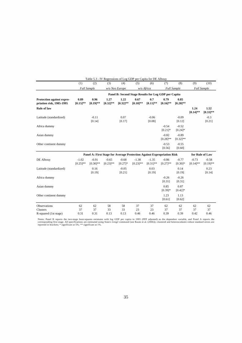
(1) (2) (3) (4) (5) (6) (7) (8) (9) (10)


Rule of law 1.24 1.52[0.14]** [0.33]**


Africa dummy -0.54 -0.52[0.21]* [0.24]*

Asian dummy -0.82 -0.89[0.28]** [0.32]**


DE Albouy -1.02 -0.91 -0.65 -0.68 -1.38 -1.35 -0.86 -0.77 -0.73 -0.58[0.25]** [0.30]** [0.23]** [0.27]* [0.23]** [0.31]** [0.27]** [0.30]* [0.14]** [0.19]**


Africa dummy -0.26 -0.26[0.31] [0.31]

Asian dummy 0.85 0.87[0.39]* [0.42]*





Table 5.3 - IV Regressions of Log GDP per Capita for DE Albouy



35

(1) (2) (3) (4) (5) (6) (7) (8) (9) (10)


Rule of law 1.26 1.61[0.15]** [0.39]**


Africa dummy -0.53 -0.5[0.22]* [0.25]*

Asian dummy -0.83 -0.91[0.28]** [0.33]**


DE Albouy Adjusted -1.12 -0.97 -0.68 -0.71 -1.5 -1.48 -0.93 -0.83 -0.81 -0.61[0.28]** [0.34]** [0.23]** [0.30]* [0.29]** [0.43]** [0.31]** [0.35]* [0.16]** [0.22]**


Africa dummy -0.32 -0.32[0.31] [0.31]

Asian dummy 0.9 0.91[0.42]* [0.45]*





Table 5.4 - IV Regressions of Log GDP per Capita for DE Albouy Adjusted



36

8 Robustness Tests

In the 8 tables of this section, I provide additional evidence that the results presented so far are

robust to the inclusion of further geographic, sociological and economic controls. In all the 80

additional robustness tests, the instruments for institutions as well as instrumented institutions

themselves are significant. In Tables 6.1 to 6.4, I present the robustness tests of Table 5 of Ace-

moglu et al. Again, this is done for my 4 measures of disease environment constructed from Table

1. In Tables 7.1 to 7.4, I present further robustness tests adding geographic and socioeconomic

controls.

In Tables 6.1 to 6.4, I first include dummies for British and French colonies from La Porta

et al. (1999) and (1998). Again, to control for the direct effects of geography, this is done with

(Column 1) and without (Column 2) adding latitude to the estimation. I find that the colony

dummies significantly influence on development, yet that they influence institutions (first stage)

and income directly (second stage) in opposing ways. To check that the colonial origins theory

of Acemoglu et. al. is also valid within the groups of former British colonies, Columns 3 and

4 restrict the sample to the 23 former British colonies. In the next two specifications, I include

a French legal origin dummy, which is again significantly negative in the first and significantly

positive in the second stage. Combining the two effects, French legal origins are on average

associated with a very small effect on income. The same finding of two counteracting effects

in the first and the second stage is true when testing for religion (Column 7 and 8 that add the

percentage of the population of Catholic and the percentage of the population of Muslim believes)

or including a French colony dummy and a French legal origin dummy at the same time (Column

9 and 10). However, regardless of which measure I control for, the first stage coefficient of disease

environment is significant and instrumented institutions are a significant determinant of economic

prosperity.

In Tables 7.1 to 7.4, I include further geographic and sociological controls. I first include the

Geographic potential for mortality, Malaria Ecology, from Kiszewski et al. (2004) in Column

1 and 2. Higher potential for malaria is associated with both worse institutional outcomes and

lower income directly, but neither effect is significant. Combining first and second stage effects and

incorporating the fact that within the sample of Acemoglu et al., the standard deviation of Malaria

Ecology is 8.43, a one standard deviation difference in this measure leads to a difference in log

income of 0.2. A dummy for landlocked countries (Column 3 and 4) is significantly detrimental for

37

institutional outcomes. Incorporating also the insignificant and positive coefficient in the second

stage, being landlocked is associated (in Table 7.1, Column 3) with a 0.62 log points lower in

income per capita, which is quite substantial. Next, in Column 5 and 6, I add an oil dummy

that equals 1 if proven oil reserves are larger than 500,000 Barrels per capita. This is the case in

Gabon, Mexico, and Venezuela. (The large oil reserves of Canada are not accounted for in Parker

(1997)). Not surprising, oil rich countries are on average richer. More surprisingly, in the sample

examined here, this effect seems to work through institutions rather than directly.

In the last four columns of Tables 7.1 to 7.4, I control for the three measures of Ethnic (Column

6), Linguistic (7), and Religious (8) Fractionalization from Alesina et al. (2003). Following the

pioneering work of Mauro (1995), low scores for these measures (low scores imply homogenous

countries) are thought to ease collaboration between groups and individuals in a country, and

thereby improve institutional outcomes. I do find some support for this view only when I include

all three measures of fractionalization at the same time (Column 10), and I also do find that only

ethnic fractionalization has a significant influence on institutions. I also find in both Column 8

and 10 that linguistic fractionalization has negative direct effects on income levels.

38

(1) (2) (3) (4) (5) (6) (7) (8) (9) (10)

Protection against expro- 0.91 0.91 0.85 0.92 0.92 0.94 0.79 0.75 0.93 0.95priation risk, 1985-1995 [0.14]** [0.17]** [0.14]** [0.20]** [0.13]** [0.16]** [0.09]** [0.12]** [0.14]** [0.18]**

Latitude (standardized) 0 -0.13 -0.02 0.06 -0.03[0.11] [0.14] [0.11] [0.12] [0.12]

Bristish colony dummy -0.55 -0.55[0.29] [0.30]

French colony dummy 0.06 0.06 0.04 0.06[0.32] [0.34] [0.26] [0.30]

French legal origin dummy 0.76 0.77 0.76 0.76[0.28]** [0.30]* [0.26]** [0.29]**

% of population Muslim 0.003 0.002[0.004] [0.004]

% of population Catholic 0.013 0.012[0.003]** [0.004]**

DE AJR -0.86 -0.76 -1.08 -0.93 -0.9 -0.82 -0.96 -0.84 -0.86 -0.75[0.17]** [0.20]** [0.21]** [0.30]** [0.17]** [0.20]** [0.17]** [0.21]** [0.18]** [0.21]**

Latitude (standardized) 0.16 0.26 0.15 0.18 0.19[0.15] [0.19] [0.15] [0.16] [0.16]

Bristish colony dummy 0.7 0.67[0.30]* [0.29]*

French colony dummy -0.51 -0.58 -0.6 -0.67[0.35] [0.37] [0.31] [0.32]*

French legal origin dummy -0.71 -0.71 -0.57 -0.56[0.32]* [0.31]* [0.32] [0.31]

% of population Muslim -0.007 -0.009[0.005] [0.006]

% of population Catholic -0.011 -0.012[0.004]* [0.004]**



Panel A: First Stage for Average Protection Against Expropriation Risk

Table 6.1 - IV Regressions of Log GDP per Capita with Additional Controls for DE AJR

Full Sample British Colonies Full Sample

Notes: Panel B reports the two-stage least-squares estimates with log GDP per capita in 1995 (PPP adjusted) as the dependent variable, and Panel A reports thecorresponding first stage. The omitted group in Columns 1 and 2 is all countries that were neither French nor British colonies. All specifications are estimated using Stata's ivreg2 command (see Baum et al. (2006)); clustered and heteroscedastic-robust standard errors are reported in brackets; * significant at 5%; ** significant at 1%.

39

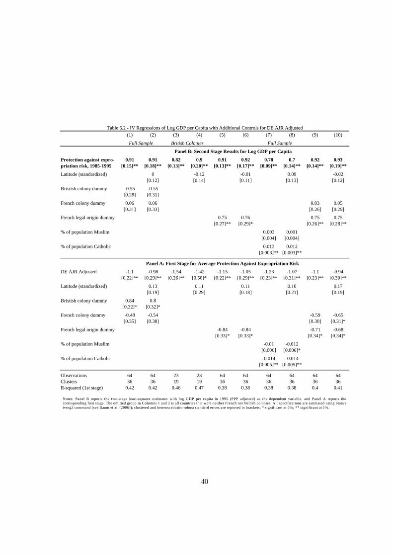
(1) (2) (3) (4) (5) (6) (7) (8) (9) (10)


Latitude (standardized) 0 -0.12 -0.01 0.09 -0.02[0.12] [0.14] [0.11] [0.13] [0.12]

Bristish colony dummy -0.55 -0.55[0.28] [0.31]


French legal origin dummy 0.75 0.76 0.75 0.75[0.27]** [0.29]* [0.26]** [0.28]**



DE AJR Adjusted -1.1 -0.98 -1.54 -1.42 -1.15 -1.05 -1.23 -1.07 -1.1 -0.94[0.22]** [0.29]** [0.26]** [0.50]* [0.22]** [0.29]** [0.23]** [0.31]** [0.23]** [0.30]**


Bristish colony dummy 0.84 0.8[0.32]* [0.32]*


French legal origin dummy -0.84 -0.84 -0.71 -0.68[0.33]* [0.33]* [0.34]* [0.34]*

% of population Muslim -0.01 -0.012[0.006] [0.006]*

% of population Catholic -0.014 -0.014[0.005]** [0.005]**




Table 6.2 - IV Regressions of Log GDP per Capita with Additional Controls for DE AJR Adjusted



40

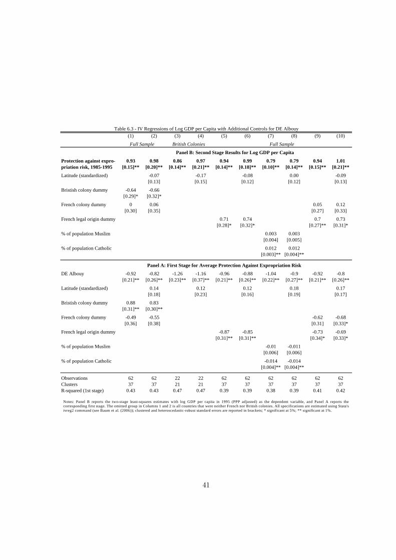
(1) (2) (3) (4) (5) (6) (7) (8) (9) (10)


Latitude (standardized) -0.07 -0.17 -0.08 0.00 -0.09[0.13] [0.15] [0.12] [0.12] [0.13]

Bristish colony dummy -0.64 -0.66[0.29]* [0.32]*

French colony dummy 0 0.06 0.05 0.12[0.30] [0.35] [0.27] [0.33]

French legal origin dummy 0.71 0.74 0.7 0.73[0.28]* [0.32]* [0.27]** [0.31]*



DE Albouy -0.92 -0.82 -1.26 -1.16 -0.96 -0.88 -1.04 -0.9 -0.92 -0.8[0.21]** [0.26]** [0.23]** [0.37]** [0.21]** [0.26]** [0.22]** [0.27]** [0.21]** [0.26]**


Bristish colony dummy 0.88 0.83[0.31]** [0.30]**


French legal origin dummy -0.87 -0.85 -0.73 -0.69[0.31]** [0.31]** [0.34]* [0.33]*

% of population Muslim -0.01 -0.011[0.006] [0.006]





Table 6.3 - IV Regressions of Log GDP per Capita with Additional Controls for DE Albouy



41

(1) (2) (3) (4) (5) (6) (7) (8) (9) (10)

Protection against expro- 0.93 1 0.85 0.98 0.94 1 0.79 0.79 0.94 1.03priation risk, 1985-1995 [0.16]** [0.21]** [0.14]** [0.21]** [0.14]** [0.19]** [0.10]** [0.15]** [0.16]** [0.22]**

Latitude (standardized) -0.08 -0.18 -0.08 0.00 -0.1[0.13] [0.15] [0.12] [0.12] [0.14]

Bristish colony dummy -0.64 -0.68[0.29]* [0.33]*


French legal origin dummy 0.71 0.75 0.7 0.74[0.28]* [0.32]* [0.27]** [0.31]*



DE Albouy Adjusted -1.02 -0.91 -1.47 -1.43 -1.07 -0.98 -1.15 -0.98 -1.01 -0.87[0.23]** [0.30]** [0.26]** [0.48]** [0.23]** [0.30]** [0.24]** [0.31]** [0.24]** [0.30]**


Bristish colony dummy 0.94 0.9[0.32]** [0.32]**


French legal origin dummy -0.94 -0.92 -0.8 -0.75[0.32]** [0.32]** [0.34]* [0.34]*

% of population Muslim -0.011 -0.013[0.006]* [0.006]*





Table 6.4 - IV Regressions of Log GDP per Capita with Additional Controls for DE Albouy Adjusted



42

(1) (2) (3) (4) (5) (6) (7) (8) (9) (10)


Malaria Ecology -0.19 -0.2(standardized) [0.13] [0.13]

Latitude (standardized) -0.03 -0.01 -0.01[0.10] [0.12] [0.12]

Religious fractionalization -0.7 -0.31[0.45] [0.40]

Linguistic fractionalization -1.01 -1.19[0.32]** [0.38]**

Ethnic fractionalization -0.76 0.58[0.41] [0.48]

Oil dummy 0.08 0.08(reserves > 500,000 b /pop) [0.25] [0.29]

Landlocked dummy 0.44 0.45[0.37] [0.38]

DE Albouy Adjusted -0.96 -0.88 -0.92 -0.83 -0.98 -0.88 -0.93 -0.95 -0.95 -0.81[0.23]** [0.26]** [0.20]** [0.22]** [0.21]** [0.24]** [0.21]** [0.20]** [0.19]** [0.18]**

Malaria Ecology -0.01 0(standardized) [0.17] [0.17]

Latitude (standardized) 0.152 0.15 0.18[0.169] [0.16] [0.17]

Religious fractionalization 0.48 0.94[0.58] [0.66]

Linguistic fractionalization 0.11 0.69[0.47] [0.62]

Ethnic fractionalization -0.36 -1.88[0.64] [0.74]*

Oil dummy 1.22 1.29(reserves > 500,000 b /pop) [0.52]* [0.56]*

Landlocked dummy -1.26 -1.26[0.40]** [0.38]**




Table 7.1 - Robustness Checks for the IV Regressions of Log GDP per Capita for DE AJR

(1), (2) w/o Malta Full sample (8), (10) w/o Haiti, El Salvador

Notes: Panel B reports the two-stage least-squares estimates with log GDP per capita in 1995 (PPP adjusted) as the dependent variable, and Panel A reports the correspondingfirst stage. Malaria Ecology is a measure of the geographic potential for malaria from Kiszewski et al. (2004). The three measures of fractionalisation are taken from Alesina et al. (2003). All specifications are estimated using Stata's ivreg2 command (see Baum et al. (2006)); clustered and heteroscedastic-robust standard errors are reported in brackets; * significant at 5%; ** significant at 1%.

43

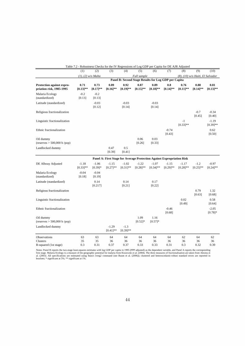
(1) (2) (3) (4) (5) (6) (7) (8) (9) (10)





Linguistic fractionalization -1 -1.19[0.33]** [0.39]**




DE Albouy Adjusted -1.18 -1.06 -1.15 -1.02 -1.22 -1.07 -1.15 -1.17 -1.2 -0.97[0.33]** [0.39]* [0.27]** [0.31]** [0.28]** [0.34]** [0.29]** [0.28]** [0.25]** [0.24]**





Ethnic fractionalization -0.46 -2.05[0.68] [0.78]*

Oil dummy 1.09 1.16(reserves > 500,000 b /pop) [0.52]* [0.57]*





Table 7.2 - Robustness Checks for the IV Regressions of Log GDP per Capita for DE AJR Adjusted



44

(1) (2) (3) (4) (5) (6) (7) (8) (9) (10)





Linguistic fractionalization -0.85 -1.07[0.36]* [0.43]*


Oil dummy 0.01 -0.13(reserves > 500,000 b /pop) [0.26] [0.32]


DE Albouy Adjusted -0.99 -0.89 -0.98 -0.87 -1.03 -0.89 -0.98 -1.01 -1.01 -0.84[0.31]** [0.35]* [0.24]** [0.28]** [0.27]** [0.31]** [0.26]** [0.25]** [0.24]** [0.24]**





Ethnic fractionalization -0.42 -2.03[0.71] [0.74]**






Table 7.3 - Robustness Checks for the IV Regressions of Log GDP per Capita for DE Albouy



45

(1) (2) (3) (4) (5) (6) (7) (8) (9) (10)





Linguistic fractionalization -0.84 -1.07[0.37]* [0.44]*


Oil dummy -0.01 -0.2(reserves > 500,000 b /pop) [0.27] [0.35]


DE Albouy Adjusted -1.05 -0.92 -1.06 -0.93 -1.12 -0.94 -1.06 -1.08 -1.11 -0.89[0.35]** [0.41]* [0.27]** [0.31]** [0.30]** [0.35]* [0.30]** [0.28]** [0.27]** [0.27]**



Religious fractionalization 0.89 1.39[0.62] [0.68]*


Ethnic fractionalization -0.46 -2.09[0.74] [0.77]**






Table 7.4 - Robustness Checks for the IV Regressions of Log GDP per Capita for DE Albouy Adjusted



46

9 Additional Instruments and Overidentification Tests

In this section, I introduce further instruments for institutions and check whether the instrumented

institutional scores are mutually consistent, i.e., I test the overidentified system. The additional

instruments I use are scores of democracy in the early 19th century (the "Polity" score and the

score for "Constraints on the Executive" from the Polity IV database), colonial and legal origin

dummies and the fraction of the population from European descent.

The results are reported in the now familiar way, where Panel A of Tables 8.1 to 8.4 reports the

first stage results with the new instruments included. In all but one specification, the measure of

disease environment is a significant instrument, while most of the additional instruments are not

significant determinants of property rights institutions. Panel C reports the instrumented second

stage, again with similar results as in earlier specifications: institutions are a major determinant of

economic performance. In Panel B, I report the overidentification tests. Since heteroscedasticity

is a potential concern, I do not report a Hausman test for the overidentification restriction, but I

report the Sargan-Hansen C-statistic for the orthogonality of the measures of disease environment

(also the Hausman test does not reject in any specification).

In the 10 instrumental variable estimations for each of the four measures of disease environment

of Tables 8.1 to 8.4, I first include the percentage of population in 1975 that is of European

descent in Column 1. This is done to address the worry that the results presented so far are

simply resulting from the fact that Europeans brought with them a culture geared towards better

property rights protection (or brought with them more human capital as is the theory of Glaeser

et al. (2004)). The fraction of the population from Europe is never a significant determinant of

institutional quality. Additionally, the overidentification test are of extremely low power, with

the lowest p-value in any of the Columns 1 equal to 0.44. In addition to testing the exclusion

restriction, I also control for the direct effects geography has on development by adding latitude

in Column 2. I find no different results than in Column 1, except that there is one case (Table

8.4, Column 2) in which the measure of disease environment is not significant when the additional

instrument is included.

I next introduce two measures of early institutional measure. Following Acemoglu et al., I

first focus on the early Polity score from the Polity IV data base as an additional instrument.

This measure takes values between -10 and +10 and is higher for more democratic societies. In

Column 3 of each of the Tables in this section, I include all countries with an available Polity

47

score in the period of 1900 to 1910 (I use the earliest available score). Few countries in the sample

of former colonies were independent at that time and there are thus only 25 observations. While

the policy score is not significant, disease environment is and again, the overidentification test

does not reject. I repeat this estimation in Column 4, but this time I include all countries with

an available Polity score before 1961, hence yielding 48 countries, and similar results as in the

previous specification. In Column 4, I again always use the earliest available Polity score after

1900 given that one was available before 1961.

Next, in Columns 5 and 6 of Tables 8.1 to 8.4, I repeat this exercise, but I focus on a sub-

indicator of the Polity database, "Constraint on the Executive." This variable takes values between

1 and 7 and measures whether superimposed structures and rules effectively constrain the exec-

utive. I again include first all countries that have a Polity score in the period of 1900 to 1910

and still exist today (Column 5) and then those with a polity score before 1961 (Column 6). In

both regressions, constraints on the executive are not significant, disease environment is, and the

overidentification test does not reject.

I next add colony dummies (Columns 7 and 8) and a French colony and legal origin dummy

(columns 9 an 10). When including a French and British colony dummy in Columns 7 and 8, I find

that the British colony dummy is always positive and always significant, while the French colony

dummy is always negative, but never significant. When including a French legal origin dummy

and a French colony dummy, both are negative and sometimes significantly so. Also in Columns

7 to 10, disease environment is significant also when the respective instruments are included, and

the overidentification test never rejects.

Overall, I conclude that the exclusion restriction that disease environment matters for in-

stitutions only indirectly through settler mortality is never rejected when adding various other

instruments for institutions while also controlling for the direct effects of geography by including

latitude.

48

(1) (2) (3) (4) (5) (6) (7) (8) (9) (10)

1911 1961 1911 1961


Latitude -0.02 0.08 0.09[0.12] [0.09] [0.10]

p-value Sargan C statistic 0.442 0.387 0.565 0.578 0.531 0.275 0.131 0.25 0.118 0.225for DE AJR

DE AJR -0.76 -0.75 -1.28 -1.03 -1.23 -1 -0.86 -0.76 -0.86 -0.75[0.25]** [0.27]** [0.17]** [0.21]** [0.20]** [0.21]** [0.17]** [0.20]** [0.18]** [0.21]**


% European descent (1975) 0.01 0.01[0.01] [0.01]

Earliest Polity score 0.04 0.02[0.03] [0.03]

Earliest executive const. 0.13 0.08[0.08] [0.08]

French legal origin dummy -0.57 -0.56[0.32] [0.31]

British colony dummy 0.7 0.67[0.30]* [0.29]*



Panel C: Second Stage Results for Log GDP per Capita

Panel B: Overidentification Tests


Table 8.1 - Overidentification Tests for DE AJR

Full Sample Polity Score Available Before Full Sample

Notes: Panel C reports the two-stage least-squares estimates with log GDP per capita in 1995 (PPP adjusted) as the dependent variable, and Panel A reports the correspondingfirst stage. Panel B reports the p-value for the null hypothesis that the coefficient on average protection against expropriation (in Panel C) is the same when instrumented using the measure of disease environment in addition to the respective instruments. The C Statistic (difference-in-Sargan) is reported. All specifications are estimated using Stata's ivreg2 command (see Baum et al. (2006)); clustered and heteroscedastic-robust standard errors are reported in brackets; * significant at 5%; ** significant at 1%.

49

(1) (2) (3) (4) (5) (6) (7) (8) (9) (10)

1911 1961 1911 1961


Latitude -0.05 0.09 0.12[0.13] [0.09] [0.10]

p-value Sargan C statistic 0.559 0.532 0.587 0.500 0.537 0.229 0.124 0.293 0.120 0.289for DE AJR Adjusted

DE AJR Adjusted -0.85 -0.84 -1.56 -1.22 -1.5 -1.19 -1.1 -0.98 -1.1 -0.94[0.31]** [0.37]* [0.23]** [0.28]** [0.30]** [0.28]** [0.22]** [0.29]** [0.23]** [0.30]**





French legal origin dummy -0.71 -0.68[0.34]* [0.34]*

British colony dummy 0.84 0.8[0.32]* [0.32]*






Table 8.2 - Overidentification Tests for DE AJR Adjusted



50

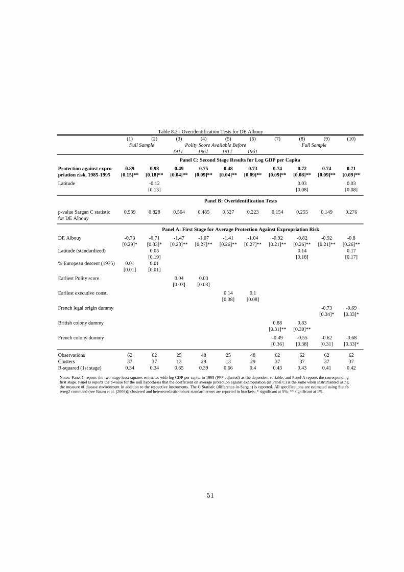
(1) (2) (3) (4) (5) (6) (7) (8) (9) (10)

1911 1961 1911 1961


Latitude -0.12 0.03 0.03[0.13] [0.08] [0.08]

p-value Sargan C statistic 0.939 0.828 0.564 0.485 0.527 0.223 0.154 0.255 0.149 0.276for DE Albouy

DE Albouy -0.73 -0.71 -1.47 -1.07 -1.41 -1.04 -0.92 -0.82 -0.92 -0.8[0.29]* [0.33]* [0.23]** [0.27]** [0.26]** [0.27]** [0.21]** [0.26]** [0.21]** [0.26]**






British colony dummy 0.88 0.83[0.31]** [0.30]**






Table 8.3 - Overidentification Tests for DE Albouy



51

(1) (2) (3) (4) (5) (6) (7) (8) (9) (10)

1911 1961 1911 1961


Latitude -0.14 0.03 0.04[0.14] [0.08] [0.08]

p-value Sargan C statistic 0.920 0.982 0.576 0.444 0.531 0.199 0.144 0.244 0.144 0.279for DE Albouy Adjusted

DE Albouy Adjusted -0.73 -0.71 -1.6 -1.12 -1.53 -1.1 -1.02 -0.91 -1.01 -0.87[0.30]* [0.35] [0.25]** [0.30]** [0.31]** [0.30]** [0.23]** [0.30]** [0.24]** [0.30]**






British colony dummy 0.94 0.9[0.32]** [0.32]**






Table 8.4 - Overidentification Tests for DE Albouy Adjusted



52

10 Conclusion

This paper does neither assess whether Daron Acemoglu, Simon Johnson or James Robinson

are consistent when they assemble their settler mortality data, nor does it examine the data

revisions of David Albouy. For many countries, there are both multiple mortality rates within a

given historical source such as Curtin (1998), as well as multiple mortality rates across historical

sources. Thus, I argue that a discussion of how to choose mortality rates is somewhat pointless:

one can never be sure that all possible historical sources of mortality rates have been exhausted,

and therefore the validity of the colonial origins theory cannot be established beyond any doubt

when using historical data.

The main contribution of this paper is to instrument for historical settler mortality rates with

a geographic model of the determinants of mortality during colonization. The geographic variables

used in this study — such as average temperature or rainfall — are measured precisely, are shown to

be strongly related to mortality and the constructed instruments are also shown to be otherwise

excludable to institutional outcomes.

After establishing the validity of my instruments, I repeat the analysis of Acemoglu et al. I

find strong support for their theory of the colonial origins of comparative development. First,

I show that the relation between institutional outcomes and the instrumented mortality rate is

highly significant in both the sample of Acemoglu et al. and when using the data constructed

by Albouy. The latter finding is robust to inclusion of controls and to accounting for the pop-

ulation the historical data was collected from (bishops, from forced labor or during campaign).

Second, I establish the effect institutions have on international income differentials by using the

constructed measures of disease environment to instrument for institutional outcomes. I find that

for all measures of early disease environment constructed in this paper, institutions are a highly

significant determinant of economic prosperity. In addition, my point estimates are similar to the

ones of Acemoglu et al. I thus conclude that their results indeed do reflect the "early institution

building" channel rather than measurement error, as is asserted by Albouy.

While I do not check the rules according to which the data is assembled, I show that the

discrepancies between the two mortality series vanish when instrumenting in the proposed way.

Although the two mortality series differ substantially, they are both affected by geography in a

very similar way. Correspondingly, for both the results relating mortality to institutions and for

the results relating institutions to income, it does not matter which series is instrumented for to

53

generate the geographic projection of mortality. Both show that the colonial origins theory is

statistically valid and economically highly relevant. Moreover, although I find that one aspect of

David Albouy’s critique is supported by the data (the "comparability problem"), accounting for

the population the mortality rate was sampled from does not change the effect institutions have

on prosperity.

This paper also has a second contribution because the developed instruments allow for an

additional falsification exercise to disentangle the colonial origins theory from the potential direct

effect disease environment may have had on institutional development. The geographic view of

development (advocated for example by Gallup et al. (1998)) predicts that there should be a rela-

tion between disease environment and economic development in all countries equally. In contrast,

the colonial origins theory predicts a relation between disease environment and development only

in the group of former colonies. My measures of early disease environment can be constructed also

for countries that have not been colonized and I can thus show that early disease environment did

influence institutional development in former colonies, yet not in a sample of countries that have

not been colonized. This differential effect disease environment has had on economic development

can only be rationalized in the context of the colonial origins theory brought forward by Acemoglu

et al.

54

References

[1] Acemoglu, Daron; Johnson, Simon and Robinson, James A. "The Colonial Origins

of Comparative Development: An Empirical Investigation" The American Economic Review,

December 2001, 91(5), pp. 1369-1401.

[2] Acemoglu, Daron; Johnson, Simon and Robinson, James A. "Disease and Develop-

ment in Historical Perspective," Journal of the European Economic Association Papers and

Proceedings, April 2003, 1, pp. 397-405

[3] Acemoglu, Daron; Johnson, Simon and Robinson, James A. "A response to Al-

bouy’s "A Reexamination Based on Improved Settler Mortality Data"" MIT Department of

Economics MIMEO, March 2005.

[4] Acemoglu, Daron; Johnson, Simon and Robinson, James A. "Reply to the Revised

(May 2006) version of David Albouy’s "The Colonial Origins of Comparative Development:

An Investigation of the Settler Mortality Data"" MIT Department of Economics MIMEO,

September 2006.

[5] Albouy, David. "The Colonial Origins of Comparative Development: A Reexamination

Based on Improved Settler Mortality Data," December 2004, University of California, Berke-

ley.

[6] Albouy, David. "The Colonial Origins of Comparative Development: An Investigation of

the Settler Mortality Data," Center for International and Development Research, University

of California Berkeley, Working Paper C04’138, May 2006.

[7] Alesina, Alberto; Devleeschauwer, Arnaud; Easterly, William; Kurlat, Sergio and

Wacziarg, Romain. "Fractionalization," National Bureau of Economic Research, Working

Paper 9411, 2003.

[8] Angrist, Joshua D. and Krueger, Alan B., 1999. "Empirical strategies in labor eco-

nomics," Handbook of Labor Economics, in: O. Ashenfelter & D. Card (ed.), Handbook of

Labor Economics, edition 1, volume 3, chapter 23, pages 1277-1366, Elsevier.

55

[9] Baum, C.F.; Schaffer, M.E.; and Stillman, S., 2006. ivreg2: Stata module for ex-

tended instrumental variables/2SLS, GMM and AC/HAC, LIML and k-class regression.

(http://ideas.repec.org/c/boc/bocode/s425401.html)

[10] Bloom, David E. and Sachs, Jeffrey D. "Geography, Demography, and Economic

Growth in Africa." Brookings Papers on Economic Activity, 1998, (2), pp. 207-73.

[11] Curtin, Philipp D. Death by migration: Europe’s encounter with the tropical world in the

19th Century. New York: Cambridge University Press, 1989.

[12] Curtin, Philipp D. Disease and empire: The health of European Troops in the Conquest

of Africa. New York: Cambridge University Press, 1998.

[13] Diamond, Jared M. Guns, germs and steel: The fate of human societies. New York: W.W.

Norton & Co. 1997.

[14] Easterly, William and Levine, Ross. "Tropics, germs, and crops: the role of endowments

in economic development," January 2003, Journal of Monetary Economics, 50(1), pp. 3-39.

[15] Gallup, John L.; Mellinger, Andrew D. and Sachs, Jeffrey D. "Geography and

Economic Development." National Bureau of Economic Research, Working Paper No. 6849,

1998.

[16] Glaeser, Edward; La Porta, Rafael; Lopez-de-Silanes, Florencio; Shleifer, Andrei

"Do Institutions Cause Growth?" Journal of Economic Growth, September 2004, 9(3), pp.

271- 304.

[17] Gutierrez, Hector La Mortalite des Eveques Latino-Americains aux XVIIe et XVIII

Siecles. Annales de Demographie Historique, 29-39. 1986

[18] Hall, Robert E. and Jones, Charles I. "Why Do Some Countries Produce So Much

More Output Per Worker Than Others?," The Quarterly Journal of Economics, February

1999, 114(1), pp. 83-116.

[19] Kaufmann, Daniel; Kraay, Art and Mastruzzi, Massimo. "Governance Matters IV:

Governance Indicators for 1996-2004" World Bank Policy Research Working Paper Series,

May 2005, No. 3630

56

[20] Kiszewski, Anthony; Mellinger, Andrew; Spielman, Andrew; Malaney, Pia;

Ehrlich Sachs, Sonia and Sachs, Jeffrey D. "A Global Index of the Stability of Malaria

Transmission," American Journal of Tropical Medicine and Hygiene, May 2004, 70(5), pp.

486-498.

[21] Knack, Stephen and Keefer, Philip. "Institutions and Economic Performance: Cross-

Country Tests Using Alternative Measure." Economics and Politics, November 1995, 7(3),

pp. 207-27.

[22] La Porta, Rafael; Lopez-de-Silanes, Florencio; Shleifer, Andrei and Vishny,

Robert W. "Law and Finance," The Journal of Political Economy, December 1999, 106(6),

pp. 1113-1155.

[23] La Porta, Rafael; Lopez-de-Silanes, Florencio; Shleifer, Andrei and Vishny,

Robert W. "The Quality of Government," Journal of Law, Economics and Organization,

December 1998, 15(1),pp. 222-279.

[24] Lipset, Seymour Martin. The Political Man. The Social Basis of Politics, Garden City,

N.Y: Doubleday, 1960.

[25] Mauro, Paolo. "Corruption and Growth," The Quarterly Journal of Economics, August

1995, 110(3), pp. 681-712.

[26] McArthur, John W. and Sachs, Jeffrey. "Institutions and Geography: Comment on

Acemoglu, Johnson and Robinson," National Bureau of Economic Research, Working Paper

No. 8114, February 2001.

[27] Parker, Philip M. National cultures of the world: A statistical reference, Cross Cultural

Statistical Encyclopedia of the World, Vol. 4 Westport, CT: Greenwood Press, 1997.

[28] Rodrik, Dani; Subramanian, Arvind and Trebbi, Francesco. "Institutions rule: The

primacy of institutions over geography and integration in economic development", Journal

of Economic Growth, June 2004, 9 (2), pp. 131-165.

[29] Sachs, Jeffrey D. "Institutions Don’t Rule: Direct Effects of Geography on Per Capita

Income" National Bureau of Economic Research, Working Paper No. 9490, February 2003.

57

11 Data Appendix

11.1 Data for Former Colonies (Main Data)

Figure A 1: The relation between the logarithm of mortality from Acemoglu et al. (2001) and its geographic projection (DE AJR from Table 1, Column 1).

AGO

ARG

AUS

BFABGD

BHS

BOL

BRA

CAN

CHL

CIVCMR

COG

COL

CRIDOM

DZAECU

EGY

ETH

GAB

GHA

GIN

GMB

GTM

GUYHKG

HND HTIIDNIND JAM

KENLKA

MAR

MDGMEX

MLI

MLTMYS

NERNGANIC

NZL

PAK

PAN

PER

PRY

SDNSEN

SGP

SLE

SLV TGO

TTO

TUN

TZA

UGA

URY

USA

VEN

VNM

ZAF

ZAR

23

45

67

Pre

dict

ed D

isea

se E

nviro

nmen

t (D

E A

JR)

2 4 6 8Logarithm of Mortality from Acemoglu et al. (2001)

Mort. from Acemoglu et al. (2001) and DE AJR

AGO

ARG

AUS

BFABGD

BHS

BOL

BRA

CAN

CHL

CIVCMR

COG

COL

CRI DOM

DZA

ECU

EGY

ETH

GABGHA

GIN

GMB

GTMGUYHKGHND

HTIIDNIND JAM

KEN

LKA

MAR

MDGMEX

MLI

MLT

MYS

NER NGANIC

NZL

PAK

PAN

PERPRY

SDN SEN

SGP

SLE

SLV TGOTTO

TUN

TZAUGA

URY

USA

VEN

VNM

ZAF

ZAR

23

45

6P

redi

cted

Dis

ease

Env

ironm

ent (

DE

AJR

Adj

uste

d)

2 4 6 8Logarithm from Mortality of Acemoglu et al. (2001)

Mort. from Acemoglu et al. (2001) and DE AJR Adjusted

Figure A 2: The relation between the logarithm of mortality from Acemoglu et al. (2001) and the geographic projection adjusted for the sampling population (DE AJR Adjusted from Table 1, Column 3).

58

AGO

ARG

AUS

BFABGD

BHS

BOL

BRA

CAN

CHL

CIVCMR

COG

COL

CRI DOM

DZAECU

EGYETH

GAB

GHA

GIN

GMB

GTMGUYHKGHNDHTIIDNIND JAM

LKA

MAR

MDGMEX

MLI

MLT

MYS

NER NGANIC

NZL

PAK

PAN

PERPRY

SDNSEN

SGP

SLE

SLV TGOTTO

TUN

UGA

URY

USA

VEN

VNM

ZAF

ZAR2

34

56

7P

redi

cted

Dis

ease

Env

ironm

ent (

DE

Alb

ouy)

2 4 6 8Logarithm of Mortality from Albouy (2006) (Revision 2)

Mort. from Albouy (2006) and DE Albouy

Figure A 3: The relation between the logarithm of mortality from Albouy (2006) and the geographic projection (DE Albouy from Table 1, Column 5).

AGO

ARG

AUS

BFABGD

BHS

BOL

BRA

CAN

CHL

CIVCMR

COG

COL

CRI DOM

DZAECU

EGYETH

GAB

GHA

GIN

GMB

GTMGUY HKGHNDHTIIDN

IND JAMLKA

MAR

MDG

MEX

MLI

MLT

MYS

NER NGANIC

NZL

PAK

PAN

PERPRY

SDNSEN

SGP

SLE

SLV TGOTTO

TUN

UGA

URY

USA

VEN

VNM

ZAF

ZAR

23

45

6P

redi

cted

Dis

ease

Env

ironm

ent (

DE

Alb

ouy

Adj

uste

d)

2 4 6 8Logarithm of Mortality from Albouy (2006)

Mort. from Albouy (2006) and DE Albouy Adjusted

Figure A 4: The relation between the logarithm of mortality from Albouy (2006) and the geographic projection adjusted for the sampling population (DE Albouy Adjusted from Table 1, Column 6).

59

Country Name Worldbank Avg. Exprop. Log GPD Ln Mortality Ln Mortality DE DE DE DECode Risk per Capita Acem. et al. Albouy AJR AJR Adj. Albouy Albouy Adj.

Algeria DZA 6.50 8.39 4.359 4.359 3.756 3.016 3.796 3.401Angola AGO 5.36 7.77 5.635 5.991 5.275 4.291 5.018 4.558

Argentina ARG 6.39 9.13 4.233 4.233 3.509 3.120 3.628 3.429Australia AUS 9.32 9.90 2.146 2.646 2.604 2.300 2.877 2.673

Bahamas, The BHS 7.50 9.29 4.443 5.242 4.701 4.002 4.650 4.305Bangladesh BGD 5.14 6.88 4.268 4.268 5.548 4.476 5.401 4.890

Bolivia BOL 5.64 7.93 4.263 4.263 3.872 3.100 3.768 3.422Brazil BRA 7.91 8.73 4.263 4.263 4.520 3.905 4.501 4.193

Burkina Faso BFA 4.45 6.85 5.635 5.991 5.745 4.673 5.510 4.999Cameroon CMR 6.45 7.50 5.635 5.991 5.018 4.186 4.946 4.541

Canada CAN 9.73 9.99 2.779 2.779 2.310 2.057 2.525 2.409Chile CHL 7.82 9.34 4.233 4.233 3.278 2.624 3.351 3.002

Colombia COL 7.32 8.81 4.263 4.263 3.386 2.963 3.515 3.306Congo, Dem. Rep. ZAR 3.50 6.87 5.481 4.605 5.265 4.279 5.062 4.598

Congo, Rep. COG 4.68 7.42 5.481 4.605 5.402 4.365 5.203 4.713Costa Rica CRI 7.05 8.79 4.358 4.358 4.972 4.015 4.835 4.386

Cote d'Ivoire CIV 7.00 7.44 6.504 6.504 5.054 4.301 5.129 4.744Dominican Rep. DOM 6.18 8.36 4.868 4.868 4.754 4.067 4.713 4.372

Ecuador ECU 6.55 8.47 4.263 4.263 4.017 3.300 3.972 3.640Egypt, Arab Rep. EGY 6.77 7.95 4.217 3.207 4.956 4.031 4.683 4.256

El Salvador SLV 5.00 7.95 4.358 4.358 5.272 4.276 5.118 4.646Ethiopia ETH 5.73 6.11 3.258 3.258 4.605 3.689 4.498 4.074Gabon GAB 7.82 8.90 5.635 5.991 5.633 4.573 5.457 4.951

Gambia, The GMB 8.27 7.27 7.293 7.293 5.569 4.467 5.437 4.913Ghana GHA 6.27 7.37 6.504 6.504 5.189 4.307 5.024 4.600

Guatemala GTM 5.14 8.29 4.263 4.263 4.787 3.843 4.646 4.208Guinea GIN 6.55 7.49 6.180 5.858 6.782 5.389 6.869 6.180Guyana GUY 5.89 7.90 3.471 4.431 4.316 3.936 4.520 4.297

Haiti HTI 3.73 7.15 4.868 4.868 4.952 4.212 4.900 4.532Honduras HND 5.32 7.69 4.358 4.556 4.975 4.017 4.773 4.328

Hong Kong (Ch) HKG 8.14 10.05 2.701 5.652 4.645 3.889 4.676 4.305India IND 8.27 7.33 3.884 3.884 5.122 4.162 4.915 4.465

Indonesia IDN 7.59 8.07 5.136 5.136 4.959 4.274 4.974 4.624Jamaica JAM 7.09 8.19 4.868 4.868 5.101 4.228 4.944 4.526Kenya KEN 6.05 7.06 4.977 na 4.416 3.613 na na

Madagascar MDG 4.45 6.84 6.284 4.317 4.645 3.746 4.546 4.127Malaysia MYS 7.95 8.89 2.874 2.874 4.007 3.826 4.326 4.183

Mali MLI 4.00 6.57 7.986 5.991 5.833 4.735 5.618 5.093Malta MLT 7.23 9.43 2.791 2.791 3.903 3.153 3.920 3.518

Mexico MEX 7.50 8.94 4.263 4.263 4.353 3.494 4.217 3.825Morocco MAR 7.09 8.04 4.359 4.359 3.964 3.212 3.965 3.563

New Zealand NZL 9.73 9.76 2.146 2.146 2.943 2.787 3.221 3.122Nicaragua NIC 5.23 7.54 5.096 5.096 5.571 4.521 5.362 4.864

Niger NER 5.00 6.73 5.991 5.991 5.634 4.594 5.374 4.881Nigeria NGA 5.55 6.81 7.603 7.603 5.461 4.557 5.422 4.974Pakistan PAK 6.05 7.35 3.611 3.611 4.887 3.999 4.767 4.347Panama PAN 5.91 8.84 5.096 5.096 5.373 4.417 5.204 4.746

Paraguay PRY 6.95 8.21 4.358 4.358 4.325 3.706 4.319 4.015Peru PER 5.77 8.40 4.263 4.263 4.779 3.873 4.522 4.107

Senegal SEN 6.00 7.40 5.104 5.104 5.626 4.572 5.392 4.892Sierra Leone SLE 5.82 6.25 6.180 5.858 6.289 5.039 6.263 5.652

Singapore SGP 9.32 10.15 2.874 2.996 2.768 3.237 3.466 3.592South Africa ZAF 6.86 8.89 2.741 2.741 3.381 2.750 3.467 3.123

Sri Lanka LKA 6.05 7.73 4.246 4.246 4.519 4.052 4.704 4.442Sudan SDN 4.00 7.31 4.480 2.389 5.489 4.491 5.196 4.726

Tanzania TZA 6.64 6.25 4.977 na 4.957 4.000 na naTogo TGO 6.91 7.22 6.504 6.504 5.189 4.307 5.024 4.600

Trinidad and Tob. TTO 7.45 8.77 4.443 4.666 4.745 4.082 4.749 4.414Tunisia TUN 6.45 8.48 4.143 4.143 3.886 3.169 3.898 3.511Uganda UGA 4.45 6.97 5.635 5.991 4.392 3.819 4.419 4.129

United States USA 10.00 10.22 2.708 2.708 2.893 2.642 3.106 2.974Uruguay URY 7.00 9.03 4.263 4.263 3.600 3.273 3.747 3.569

Venezuela, VEN 7.14 9.07 4.358 4.358 4.555 3.723 4.398 4.012Vietnam VNM 6.41 7.28 4.942 4.942 5.162 4.268 5.076 4.643

Table A1 - List of the Data (Main Analysis)

60

11.2 Data for Non-Colonies

This is the list of data used in Section 6. For these countries, the measures of mortality rates

have been predicted out of sample using the respective coefficents from Table 1.

Country Name Worldbank Rule of Avg. Exprop. DE DE DE DE Warsaw PactCode Law Risk AJR AJR Adj. Albouy Albouy Adj. Dummy

Afghanistan AFG . -1.614 3.811 2.992 3.675 3.314 0Albania ALB 7.26 -0.749 2.857 2.427 3.132 2.871 1Andorra ADO . 1.472 2.060 1.756 2.371 2.180 0Armenia ARM . -0.477 3.435 2.725 3.345 3.035 1Austria AUT 9.74 1.959 2.951 2.508 3.040 2.838 0

Azerbaijan AZE . -0.870 3.977 3.207 3.840 3.494 1Belarus BLR . -1.105 2.645 2.214 2.750 2.561 1Belgium BEL 9.69 1.497 2.910 2.568 3.063 2.898 0

Bosnia and Herz. BIH . -0.739 2.144 1.828 2.437 2.241 0Bulgaria BGR 9.04 -0.077 3.231 2.678 3.252 3.003 1

China CHN 8.11 -0.347 4.026 3.173 3.939 3.555 0Croatia HRV . -0.055 2.118 1.894 2.468 2.306 0

Czech Republic CZE 9.88 0.645 3.014 2.418 3.007 2.749 1Denmark DNK 9.72 1.962 3.053 2.552 3.100 2.875 0Estonia EST . 0.658 2.717 2.281 2.810 2.617 1Finland FIN 9.72 2.036 2.717 2.281 2.810 2.617 0France FRA 9.71 1.440 3.446 2.924 3.468 3.225 0Georgia GEO . -0.842 3.796 3.091 3.712 3.393 1Germany DEU 9.88 1.813 2.958 2.509 3.039 2.835 0Greece GRC 7.48 0.738 3.392 2.750 3.462 3.115 0

Hungary HUN 9.08 0.794 3.128 2.625 3.172 2.945 1Iceland ISL 9.70 1.926 2.642 2.252 2.774 2.599 0Ireland IRL 9.72 1.743 2.928 2.532 3.039 2.855 0

Italy ITA 9.46 0.882 3.132 2.569 3.283 2.970 0Japan JPN 9.72 1.576 3.618 3.132 3.744 3.503 0

Kazakhstan KAZ . -0.839 3.167 2.474 3.074 2.778 1Korea, Dem. Rep. PRK 5.02 -1.092 3.703 2.944 3.674 3.332 0

Korea, Rep. KOR 8.57 0.753 3.904 3.156 3.948 3.601 0Kyrgyz Republic KGZ . -0.815 2.701 2.168 2.754 2.526 1

Latvia LVA . 0.281 2.627 2.200 2.727 2.541 1Liechtenstein LIE . 1.438 2.595 2.357 2.835 2.715 0

Lithuania LTU . 0.270 2.717 2.281 2.810 2.617 1Luxembourg LUX 10.00 1.961 2.991 2.565 3.089 2.892 0

Macedonia, FYR MKD . -0.420 2.129 1.813 2.409 2.214 0Moldova MDA . -0.411 3.292 2.746 3.318 3.070 1Monaco MCO . 0.772 3.024 2.517 3.206 2.916 0

Mongolia MNG 7.95 0.247 2.513 1.844 2.481 2.209 0Nepal NPL . -0.442 4.729 3.769 4.632 4.186 0

Netherlands NLD 9.98 1.900 3.009 2.569 3.091 2.890 0Norway NOR 9.85 2.033 2.913 2.379 2.957 2.723 0Poland POL 7.81 0.549 3.010 2.501 3.067 2.839 1

Portugal PRT 9.01 1.243 3.583 2.889 3.639 3.267 0Romania ROM 7.56 -0.218 3.216 2.643 3.244 2.987 1

Russian Fed. RUS 8.50 -0.805 2.555 2.133 2.668 2.484 1San Marino SMR . 0.772 3.132 2.569 3.283 2.970 0

Saudi Arabia SAU 7.44 0.572 4.890 3.969 4.631 4.206 0Slovak Republic SVK 9.00 0.278 2.989 2.450 3.023 2.785 1

Slovenia SVN . 0.858 1.846 1.653 2.221 2.076 0Spain ESP 9.55 1.235 2.924 2.373 3.048 2.747 0

Sweden SWE 9.50 1.934 2.996 2.450 3.022 2.782 0Switzerland CHE 9.99 2.137 2.685 2.437 2.918 2.792 0

Taiwan TWN 9.24 0.949 3.946 3.535 4.143 3.918 0Tajikistan TJK . -1.316 3.987 3.177 3.834 3.473 1Thailand THA 7.64 0.296 5.605 4.578 5.413 4.922 0Turkey TUR 7.29 0.052 3.485 2.785 3.397 3.089 0

Turkmenistan TKM . -1.219 3.990 3.204 3.828 3.477 1Ukraine UKR . -0.765 2.840 2.344 2.905 2.687 1

United Kingdom GBR 9.76 1.875 3.322 2.828 3.362 3.133 0Uzbekistan UZB . -1.106 3.900 3.124 3.746 3.401 1

Yugo., Fed. Rep. YUG 6.36 -0.952 1.846 1.653 2.221 2.076 0

Table A1 - List of the Data (Falsification Exercise)

61

Swiss National Bank Working Papers published since 2004: 2004-1 Samuel Reynard: Financial Market Participation and the Apparent Instability of

Money Demand 2004-2 Urs W. Birchler and Diana Hancock: What Does the Yield on Subordinated Bank Debt Measure? 2005-1 Hasan Bakhshi, Hashmat Khan and Barbara Rudolf: The Phillips curve under state-dependent pricing 2005-2 Andreas M. Fischer: On the Inadequacy of Newswire Reports for Empirical Research on Foreign Exchange Interventions 2006-1 Andreas M. Fischer: Measuring Income Elasticity for Swiss Money Demand: What do the Cantons say about Financial Innovation? 2006-2 Charlotte Christiansen and Angelo Ranaldo: Realized Bond-Stock Correlation:

Macroeconomic Announcement Effects 2006-3 Martin Brown and Christian Zehnder: Credit Reporting, Relationship Banking, and Loan Repayment 2006-4 Hansjörg Lehmann and Michael Manz: The Exposure of Swiss Banks to

Macroeconomic Shocks – an Empirical Investigation 2006-5 Katrin Assenmacher-Wesche and Stefan Gerlach: Money Growth, Output Gaps and

Inflation at Low and High Frequency: Spectral Estimates for Switzerland 2006-6 Marlene Amstad and Andreas M. Fischer: Time-Varying Pass-Through from Import

Prices to Consumer Prices: Evidence from an Event Study with Real-Time Data 2006-7 Samuel Reynard: Money and the Great Disinflation 2006-8 Urs W. Birchler and Matteo Facchinetti: Can bank supervisors rely on market data?

A critical assessment from a Swiss perspective 2006-9 Petra Gerlach-Kristen: A Two-Pillar Phillips Curve for Switzerland 2006-10 Kevin J. Fox and Mathias Zurlinden: On Understanding Sources of Growth and

Output Gaps for Switzerland 2006-11 Angelo Ranaldo: Intraday Market Dynamics Around Public Information Arrivals

2007-1 Andreas M. Fischer, Gulzina Isakova and Ulan Termechikov: Do FX traders in Bishkek have similar perceptions to their London colleagues? Survey evidence of market practitioners’ views

2007-2 Ibrahim Chowdhury and Andreas Schabert: Federal Reserve Policy viewed through

a Money Supply Lens 2007-3 Angelo Ranaldo: Segmentation and Time-of-Day Patterns in Foreign Exchange

Markets 2007-4 Jürg M. Blum: Why ‘Basel II’ May Need a Leverage Ratio Restriction 2007-5 Samuel Reynard: Maintaining Low Inflation: Money, Interest Rates, and Policy

Stance 2007-6 Rina Rosenblatt-Wisch: Loss Aversion in Aggregate Macroeconomic Time Series 2007-7 Martin Brown, Maria Rueda Maurer, Tamara Pak and Nurlanbek Tynaev: Banking

Sector Reform and Interest Rates in Transition Economies: Bank-Level Evidence from Kyrgyzstan

2007-8 Hans-Jürg Büttler: An Orthogonal Polynomial Approach to Estimate the Term

Structure of Interest Rates 2007-9 Raphael Auer: The Colonial Origins Of Comparative Development: Comment.

A Solution to the Settler Mortality Debate

Swiss National Bank Working Papers are also available at www.snb.ch, section Publications/ResearchSubscriptions or individual issues can be ordered at Swiss National Bank, Fraumünsterstrasse 8, CH-8022 Zurich,fax +41 44 631 81 14, E-mail [email protected]

the colonial origins of comparative development: … critique focuses in particular on three issues....

Documents