The common ancestor process

revisited

Sandra Kluth, Thiemo Hustedt, Ellen Baake

Technische Fakultät, Universität Bielefeld, Box 100131, 33501 Bielefeld, Germany

E-mail: {skluth, thustedt, ebaake}@techfak.uni-bielefeld.de

Abstract. We consider the Moran model in continuous time with twotypes, mutation, and selection. We concentrate on the ancestral line and itsstationary type distribution. Building on work by Fearnhead (J. Appl. Prob.39 (2002), 38-54) and Taylor (Electron. J. Probab. 12 (2007), 808-847), wecharacterise this distribution via the fixation probability of the offspring ofall individuals of favourable type (regardless of the offsprings’ types). Weconcentrate on a finite population and stay with the resulting discrete settingall the way through. This way, we extend previous results and gain newinsight into the underlying particle picture.

2000 Mathematics Subject Classification: Primary 92D15; Secondary60J28.

Key words:Moran model, ancestral process with selection, ancestral line,common ancestor process, fixation probabilities.

1 Introduction

Understanding the interplay of random reproduction, mutation, and selection is a majortopic of population genetics research. In line with the historical perspective of evolu-tionary research, modern approaches aim at tracing back the ancestry of a sample ofindividuals taken from a present population. Generically, in populations that evolveat constant size over a long time span without recombination, the ancestral lines willeventually coalesce backwards in time into a single line of descent. This ancestral lineis of special interest. In particular, its type composition may differ substantially fromthe distribution at present time. This mirrors the fact that the ancestral line consistsof those individuals that are successful in the long run; thus, its type distribution isexpected to be biased towards the favourable types.

1

This article is devoted to the ancestral line in a classical model of population genetics,namely, the Moran model in continuous time with two types, mutation, and selection(i.e., one type is ‘fitter’ than the other). We are particularly interested in the stationarydistribution of this type process, to be called the ancestral type distribution. We buildon previous work by Fearnhead [9] and Taylor [20]. Fearnhead’s approach is based onthe ancestral selection graph, or ASG for short [14, 16]. The ASG is an extension ofKingman’s coalescent [12, 13], which is the central tool to describe the genealogy of afinite sample in the absence of selection. The ASG copes with selection by includingso-called virtual branches in addition to the real branches that define the true genealogy.Fearnhead calculates the ancestral type distribution in terms of the coefficients of a seriesexpansion that is related to the number of virtual branches.

Taylor uses diffusion theory and a backward-forward construction that relies on adescription of the full population. He characterises the ancestral type distribution interms of the fixation probability of the offspring of all ‘fit’ individuals (regardless of theoffsprings’ types). This fixation probability is calculated via a boundary value problem.

Both approaches rely strongly on analytical tools; in particular, they employ thediffusion limit (which assumes infinite population size, weak selection and mutation)from the very beginning. The results only have partial interpretations in terms of thegraphical representation of the model (i.e., the representation that makes individuallineages and their interactions explicit). The aim of this article is to complement theseapproaches by starting from the graphical representation for a population of finite sizeand staying with the resulting discrete setting all the way through, performing thediffusion limit only at the very end. This will result in an extension of the results toarbitrary selection strength, as well as a number of new insights, such as an intuitiveexplanation of Taylor’s boundary value problem in terms of the particle picture, and analternative derivation of the ancestral type distribution.

The paper is organised as follows. We start with a short outline of the Moran model(Section 2). In Section 3, we introduce the common ancestor type process and brieflyrecapitulate Taylor’s and Fearnhead’s approaches. We concentrate on a Moran modelof finite size and trace the descendants of the initially ‘fit’ individuals forward in time.Decomposition according to what can happen after the first step gives a difference equa-tion, which turns into Taylor’s diffusion equation in the limit. We solve this differenceequation and obtain the fixation probability in the finite-size model in closed form. InSection 5, we derive the coefficients of the ancestral type distribution within the discretesetting. Section 6 summarises and discusses the results.

2 The Moran model with mutation and selection

We consider a haploid population of fixed size N ∈ N in which each individual is charac-terised by a type i ∈ S = {0, 1}. If an individual reproduces, its single offspring inheritsthe parent’s type and replaces a randomly chosen individual, maybe its own parent.This way the replaced individual dies and the population size remains constant.

Individuals of type 1 reproduce at rate 1, whereas individuals of type 0 reproduce at

2

rate 1 + sN , sN > 0. Accordingly, type-0 individuals are termed ‘fit’, type-1 individualsare ‘unfit’. In line with a central idea of the ASG, we will decompose reproductionevents into neutral and selective ones. Neutral ones occur at rate 1 and happen toall individuals, whereas selective events occur at rate sN and are reserved for type-0individuals.

Mutation occurs independently of reproduction. An individual of type i mutates totype j at rate uNνj, uN > 0, 0 < νj < 1, ν0 + ν1 = 1. This is to be understood in thesense that every individual, regardless of its type, mutates at rate uN and the new typeis j with probability νj. Note that this includes the possibility of ‘silent’ mutations, i.e.mutations from type i to type i.

The Moran model has a well-known graphical representation as an interacting particlesystem (cf. Fig. 1). The N vertical lines represent the N individuals, with time runningfrom top to bottom in the figure. Reproduction events are represented by arrows withthe reproducing individual at the base and the offspring at the tip. Mutation events aremarked by bullets.

t

0

00000

0 0

1 1

1

1

1 1 1 1

Figure 1: The Moran model. The types (0 = fit, 1 = unfit) are indicated for the initialpopulation (top) and the final one (bottom).

We are now interested in the process(ZN

t

)t>0

, where ZNt is the number of individuals

of type 0 at time t. When the number of type-0 individuals is k, it increases by one atrate λNk and decreases by one at rate µN

k , where

λNk =k(N − k)

N(1 + sN) + (N − k)uNν0 and µN

k =k(N − k)

N+ kuNν1. (1)

Thus(ZN

t

)t>0

is a birth-death process with birth rates λNk and death rates µNk . For

uN > 0 and 0 < ν0, ν1 < 1 its stationary distribution is(πNZ (k)

)06k6N

with

πNZ (k) = CN

k∏

i=1

λNi−1

µNi

, 0 6 k 6 N, (2)

where CN is a normalising constant (cf. [4, p. 19]). (As usual, an empty product isunderstood as 1.)

3

To arrive at a diffusion, we consider the usual rescaling(XN

t

)t>0

:=1

N

(ZN

Nt

)t>0

,

and assume that limN→∞NuN = θ, 0 < θ <∞, and limN→∞NsN = σ, 0 6 σ <∞. AsN → ∞, we obtain the well-known diffusion limit

(Xt)t>0 := limN→∞

(XN

t

)t>0

.

Given x ∈ [0, 1], a sequence (kN)N∈N with kN ∈ {0, . . . , N} and limN→∞kN

N= x, (Xt)t>0

is characterised by the drift coefficient

a(x) = limN→∞

(λNkN

− µNkN

) = (1− x)θν0 − xθν1 + (1− x)xσ (3)

and the diffusion coefficient

b(x) = limN→∞

1

N

(λNk

N

+ µNkN

)= 2x(1− x). (4)

Hence, the infinitesimal generator A of the diffusion is defined by

Af(x) = (1− x)x∂2

∂x2f(x) + [(1− x)θν0 − xθν1 + (1− x)xσ]

∂

∂xf(x), f ∈ C2([0, 1]).

The stationary density πX – known as Wright’s formula – is given by

πX(x) = C(1− x)θν1−1xθν0−1 exp(σx), (5)

where C is a normalising constant. See [5, Ch. 7, 8] or [8, Ch. 4, 5] for reviewsof diffusion processes in population genetics and [11, Ch. 15] for a general survey ofdiffusion theory.

In contrast to our approach starting from the Moran model, [9] and [20] choose thediffusion limit of the Wright-Fisher model as the basis for the common ancestor pro-cess. This is, however, of minor importance, since both diffusion limits differ only by arescaling of time by a factor of 2 (cf. [5, Ch. 7], [8, Ch. 5] or [11, Ch. 15]).

3 The common ancestor type process

Assume that the population is stationary and evolves according to the diffusion process(Xt)t>0. Then, at any time t, there almost surely exists a unique individual that is, atsome time s > t, ancestral to the whole population; cf. Fig. 2. (One way to see this isvia [14, Thm. 3.2, Corollary 3.4], which shows that the expected time to the ultimateancestor in the ASG remains bounded if the sample size tends to infinity.) We say thatthe descendants of this individual become fixed and call it the common ancestor at timet. The lineage of these distinguished individuals over time defines the so-called ancestralline. Denoting the type of the common ancestor at time t by It, It ∈ S, we term (It)t>0

the common ancestor type process or CAT process for short. Of particular importanceis its stationary type distribution α = (αi)i∈S, to which we will refer as the ancestraltype distribution. Unfortunately the CAT process is not Markovian. But two approachesare available that augment (It)t>0 by a second component to obtain a Markov process.They go back to Fearnhead [9] and Taylor [20]; we will recapitulate them below.

4

t t

ss

t− τ0

CA

Figure 2: Left: The common ancestor at time t (CA) is the individual whose progeny willeventually fix in the population (at time s > t). Right: If we pick an arbitraryindividual at time t, there exists a minimal time τ0 so that the individual’sline of ancestors (dotted) corresponds to the ancestral line (dashed) up to timet− τ0.

3.1 Taylor’s approach

For ease of exposition, we start with Taylor’s approach [20]. It relies on a descriptionof the full population forward in time (in the diffusion limit of the Moran model asN → ∞) and builds on the so-called structured coalescent [2]. The process is (It, Xt)t>0,with states (i, x), i ∈ S and x ∈ [0, 1]. In [20] this process is termed common ancestorprocess (CAP).

Define h(x) as the probability that the common ancestor at a given time is of type 0,provided that the frequency of type-0 individuals at this time is x. Obviously h(0) = 0,h(1) = 1. Since the process is time-homogeneous, h is independent of time. Denotethe (stationary) distribution of (It, Xt)t>0 by πT . Its marginal distributions are α (withrespect to the first variable) and πX (with respect to the second variable). πT may thenbe written as the product of the marginal density πX(x) and the conditional probabilityh(x) (cf. [20]):

πT (0, x) dx = h(x)πX(x)dx,

πT (1, x) dx = (1− h(x)) πX(x)dx.

Since πX is well-known (5), it remains to specify h. Taylor uses a backward-forwardconstruction within diffusion theory to derive a boundary value problem for h, namely:

1

2b(x)h′′(x) + a(x)h′(x)−

(θν1

x

1− x+ θν0

1− x

x

)h(x) + θν1

x

1− x= 0,

h(0) = 0, h(1) = 1.(6)

Taylor shows that (6) has a unique solution. The stationary distribution of (It, Xt)t>0

is thus determined in a unique way as well. The function h is smooth in (0, 1) and itsderivative h′ can be continuously extended to [0, 1] (cf. [20, Lemma 2.3, Prop. 2.4]).

5

In the neutral case (i.e., without selection, σ = 0), all individuals reproduce at thesame rate, independently of their types. For reasons of symmetry, the common ancestorthus is a uniform random draw from the population; consequently, h(x) = x. In thepresence of selection, Taylor determines the solution of the boundary value problem viaa series expansion in σ (cf. [20, Sec. 4] and see below), which yields

h(x) = x+ σx−θν0 (1− x)−θν

1 exp(−σx)

∫ x

0

(x̃− p) pθν0 (1− p)θν1 exp(σp)dp (7)

with x̃ =

∫ 1

0pθν0+1 (1− p)θν1 exp(σp)dp∫ 1

0pθν0 (1− p)θν1 exp(σp)dp

=Eπ

X(X2(1−X))

EπX(X(1−X))

. (8)

The stationary type distribution of the ancestral line now follows via marginalisation:

α0 =

∫ 1

0

h(x)πX(x)dx and α1 =

∫ 1

0

(1− h(x)) πX(x)dx. (9)

Following [20], we define ψ(x) := h(x)− x and write

h(x) = x+ ψ(x). (10)

Since h(x) is the conditional probability that the common ancestor is fit, ψ(x) is thepart of this probability that is due to selective reproduction.Substituting (10) into (6) leads to a boundary value problem for ψ:

1

2b(x)ψ′′(x) + a(x)ψ′ (x)−

(θν1

x

1− x+ θν0

1− x

x

)ψ(x) + σx (1− x) = 0,

ψ(0) = ψ(1) = 0.

(11)

Here, the smooth inhomogeneous term is more favourable as compared to the diver-gent inhomogeneous term in (6). Note that Taylor actually derives the boundary valueproblems (6) and (11) for the more general case of frequency-dependent selection, butrestricts himself to frequency-independence to derive solution (7).

3.2 Fearnhead’s approach

We can only give a brief introduction to Fearnhead’s approach [9] here. On the basisof the ASG, the ancestry of a randomly chosen individual from the present (stationary)population is traced backwards in time. More precisely, one considers the process (Jτ )τ>0

with values in S, where Jτ is the type of the individual’s ancestor at time τ before thepresent (that is, at forward time t − τ). Obviously, there is a minimal time τ0 so that,for all τ > τ0, Jτ = It−τ (see also Fig. 2), provided the underlying process (Xt)t>0 isextended to (−∞,∞).

To make the process Markov, the true ancestor (known as the real branch) is aug-mented by a collection of virtual branches (see [1, 14, 16, 19] for the details). Following [9,Thm. 1], certain virtual branches may be removed (without compromising the Markov

6

property) and the remaining set of virtual branches contains only unfit ones. We willrefer to the resulting construction as the pruned ASG. It is described by the process(Jτ , Vτ )τ>0, where Vτ (with values in N0) is the number of virtual branches (of type 1).(Jτ , Vτ )τ>0 is termed common ancestor process in [9] (but keep in mind that it is (It, Xt)that is called CAP in [20]). Reversing the direction of time in the pruned ASG yieldsan alternative augmentation of the CAT process (for τ > τ0).

Fearnhead provides a representation of the stationary distribution of the pruned pro-cess, which we will denote by πF . This stationary distribution is expressed in terms of

constants ρ(k)1 , . . . , ρ

(k)k+1 defined by the following backward recursion:

ρ(k)k+1 = 0 and ρ

(k)j−1 =

σ

j + σ + θ − (j + θν1)ρ(k)j

, k ∈ N0, 0 6 j 6 k + 1. (12)

The limit ρj := limk→∞ ρ(k)j exists (cf. [9, Lemma 1]) and the stationary distribution of

the pruned ASG is given by (cf. [9, Thm. 3])

πF (i, n) =

{anEπ

X(X(1−X)n), if i = 0,

(an − an+1)EπX((1−X)n+1), if i = 1,

with an :=n∏

j=1

ρj

for all n ∈ N0. Fearnhead proves this result by straightforward verification of the sta-tionarity condition; the calculation is somewhat cumbersome and does not yield insightinto the connection with the graphical representation of the pruned ASG. Marginalisingover the number of virtual branches results in the stationary type distribution of theancestral line, namely,

αi =∑

n>0

πF (i, n). (13)

Furthermore, this reasoning points to an alternative representation of h respectively ψ(cf. [20]):

h(x) = x+ x∑

n>1

an(1− x)n respectively ψ(x) = x∑

n>1

an(1− x)n. (14)

The an, to which we will refer as Fearnhead’s coefficients, can be shown [20] to followthe second-order forward recursion

(2 + θν1) a2 − (2 + σ + θ) a1 + σ = 0,

(n + θν1) an − (n+ σ + θ) an−1 + σan−2 = 0, n > 3.(15)

Indeed, (14) solves the boundary problem (6) and therefore equals (7) (cf. [20, Lemma4.1]).

7

The forward recursion (15) is greatly preferable to the backward recursion (12), whichcan only be solved approximately with initial value ρn ≈ 0 for some large n. What isstill missing is the initial value, a1. To calculate it, Taylor defines (cf. [20, Sec. 4.1])

v(x) :=h(x)− x

x=ψ(x)

x=∑

n>1

an(1− x)n (16)

and uses1

an =(−1)n

n!v(n)(1). (17)

This way a straightforward (but lengthy) calculation (that includes a differentiation ofexpression (7)) yields

a1 = −v′(1) = −ψ′(1) =σ

1 + θν1(1− x̃). (18)

4 Discrete approach

Our focus is on the stationary type distribution (αi)i∈S of the CAT process. We haveseen so far that it corresponds to the marginal distribution of both πT and πF , withrespect to the first variable. Our aim now is to establish a closer connection betweenthe properties of the ancestral type distribution and the graphical representation of theMoran model. In a first step we re-derive the differential equations for h and ψ in adirect way, on the basis of the particle picture for a finite population. This derivationwill be elementary and, at the same time, it will provide a direct interpretation of theresulting differential equations.

4.1 Difference and differential equations for h and ψ

Equations for h. Since it is essential to make the connection with the graphicalrepresentation explicit, we start from a population of finite size N , rather than from thediffusion limit. Namely, we look at a new Markov process (M t, Z

Nt )t>0 where ZN

t is thenumber of fit individuals as before and M t = (M0,M1)t holds the number of descendantsof types 0 and 1 at time t of an unordered sample with composition M 0 = (M0,M1)0collected at time 0. More precisely, we start with an arbitrary state (M 0, Z

N0 ) = (m, k)

(where M 0 need not to be a random sample) and observe the population evolve inforward time. At time t, count the type-0 descendants and the type-1 descendants ofour initial sample M 0 and summarise the results in the unordered sample M t. Togetherwith ZN

t , this gives the current state (M t, ZNt ) (cf. Fig. 3).

As soon as the initial sample is ancestral to allN individuals, it clearly will be ancestralto all N individuals at all later times. Therefore

AN := {(m, k) : k ∈ {0, . . . , N}, m0 6 k, |m| = N} ,

1Note the missing factor of 1/n in his equation (28).

8

t

00

0 0 01

1111

1 1((2, 2), 3)

((1, 3), 2)

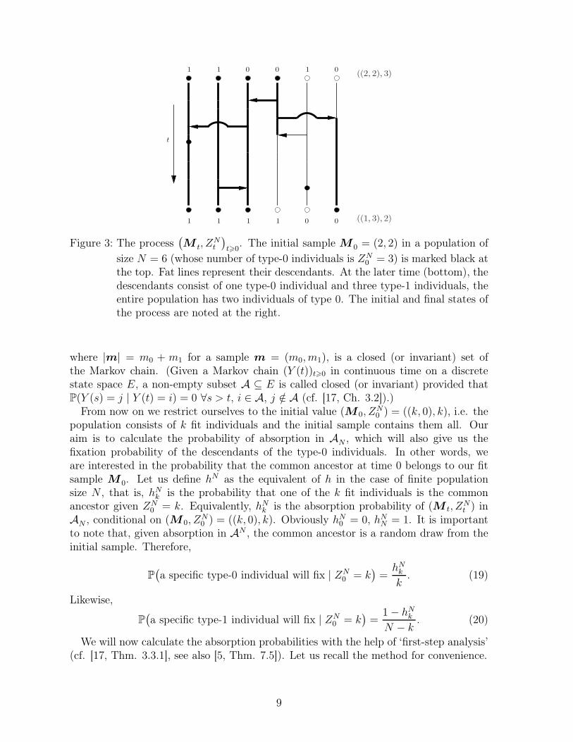
Figure 3: The process(M t, Z

Nt

)t>0

. The initial sample M 0 = (2, 2) in a population of

size N = 6 (whose number of type-0 individuals is ZN0 = 3) is marked black at

the top. Fat lines represent their descendants. At the later time (bottom), thedescendants consist of one type-0 individual and three type-1 individuals, theentire population has two individuals of type 0. The initial and final states ofthe process are noted at the right.

where |m| = m0 + m1 for a sample m = (m0, m1), is a closed (or invariant) set ofthe Markov chain. (Given a Markov chain (Y (t))t>0 in continuous time on a discretestate space E, a non-empty subset A ⊆ E is called closed (or invariant) provided thatP(Y (s) = j | Y (t) = i) = 0 ∀s > t, i ∈ A, j /∈ A (cf. [17, Ch. 3.2]).)

From now on we restrict ourselves to the initial value (M 0, ZN0 ) = ((k, 0), k), i.e. the

population consists of k fit individuals and the initial sample contains them all. Ouraim is to calculate the probability of absorption in AN , which will also give us thefixation probability of the descendants of the type-0 individuals. In other words, weare interested in the probability that the common ancestor at time 0 belongs to our fitsample M 0. Let us define hN as the equivalent of h in the case of finite populationsize N , that is, hNk is the probability that one of the k fit individuals is the commonancestor given ZN

0 = k. Equivalently, hNk is the absorption probability of (M t, ZNt ) in

AN , conditional on (M 0, ZN0 ) = ((k, 0), k). Obviously hN0 = 0, hNN = 1. It is important

to note that, given absorption in AN , the common ancestor is a random draw from theinitial sample. Therefore,

P(a specific type-0 individual will fix | ZN

0 = k)=hNkk. (19)

Likewise,

P(a specific type-1 individual will fix | ZN

0 = k)=

1− hNkN − k

. (20)

We will now calculate the absorption probabilities with the help of ‘first-step analysis’(cf. [17, Thm. 3.3.1], see also [5, Thm. 7.5]). Let us recall the method for convenience.

9

Lemma 1 (‘first-step analysis’). Assume that (Y (t))t>0 is a Markov chain in continuoustime on a discrete state space E, A ⊆ E is a closed set and Tx, x ∈ E, is the waitingtime to leave the state x. Then for all y ∈ E,

P (Y absorbs in A | Y (0) = y) =∑

z∈E:z 6=y

P (Y (Ty) = z | Y (0) = y)

× P (Y absorbs in A | Y (0) = z) .

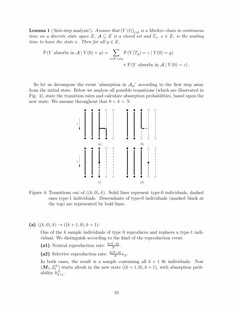
So let us decompose the event ‘absorption in AN ’ according to the first step awayfrom the initial state. Below we analyse all possible transitions (which are illustrated inFig. 4), state the transition rates and calculate absorption probabilities, based upon thenew state. We assume throughout that 0 < k < N .

(a) (b)

(c) (d)

t

t

Figure 4: Transitions out of ((k, 0), k). Solid lines represent type-0 individuals, dashedones type-1 individuals. Descendants of type-0 individuals (marked black atthe top) are represented by bold lines.

(a) ((k, 0), k) → ((k + 1, 0), k + 1):

One of the k sample individuals of type 0 reproduces and replaces a type-1 indi-vidual. We distinguish according to the kind of the reproduction event.

(a1) Neutral reproduction rate: k(N−k)N

.

(a2) Selective reproduction rate: k(N−k)N

sN .

In both cases, the result is a sample containing all k + 1 fit individuals. Now(M t, Z

Nt ) starts afresh in the new state ((k + 1, 0), k + 1), with absorption prob-

ability hNk+1.

10

(b) ((k, 0), k) → ((k − 1, 0), k − 1) :A type-1 individual reproduces and replaces a (sample) individual of type 0. This

occurs at rate k(N−k)N

and leads to a sample that consists of all k−1 fit individuals.The absorption probability, if we start in the new state, is hNk−1.

(c) ((k, 0), k) → ((k − 1, 1), k − 1):This transition describes a mutation of a type-0 individual to type 1 and occursat rate kuNν1. The new sample contains all k − 1 fit individuals, plus a singleunfit one. Starting now from

((k − 1, 1), k − 1

), the absorption probability has

two contributions: First, by definition, with probability hNk−1, one of the k − 1 fitindividuals will be the common ancestor. In addition, by (20), the single unfitindividual has fixation probability (1− hNk−1)/(N − (k − 1)), so the probability toabsorb in AN when starting from the new state is

P(absorption in AN |

(M 0, Z

N0

)= ((k − 1, 1), k − 1)

)

= hNk−1 +1− hNk−1

N − (k − 1).

(d) ((k, 0), k) → ((k, 0), k + 1):This is a mutation from type 1 to type 0, which occurs at rate (N − k)uNν0. Wethen have k + 1 fit individuals in the population altogether, but the new samplecontains only k of them. Arguing as in (c) and this time using (19), we get

P(absorption in AN |

(M 0, Z

N0

)= ((k, 0), k + 1)

)

= hNk+1 −hNk+1

k + 1.

Note that, in steps (c) and (d) (and already in (19) and (20)), we have used the permuta-tion invariance of the fit (respectively unfit) lines to express the absorption probabilitiesas a function of k (the number of fit individuals in the population) alone. This way,we need not cope with the full state space of (M t, Z

Nt ). Taking together the first-step

principle with the results of (a)–(d), we obtain the linear system of equations for hN

(with the rates λNk and µNk as in (1)):

(λNk + µN

k

)hNk = λNk h

Nk+1 + µN

k hNk−1 + kuNν1

1− hNk−1

N − (k − 1)− (N − k)uNν0

hNk+1

k + 1, (21)

0 < k < N , which is complemented by the boundary conditions hN0 = 0, hNN = 1.Rearranging results in

1

2

1

N

(λNk + µN

k

)N2(hNk+1 − 2hNk + hNk−1

)

+1

2

(λNk − µN

k

) (N(hNk+1 − hNk

)−N

(hNk−1 − hNk

))

+k

N

N

N − (k − 1)NuNν1

(1− hNk−1

)−N − k

N

N

k + 1NuNν0h

Nk+1 = 0.

(22)

11

Let us now consider a sequence (kN)N∈N with 0 < kN < N and limN→∞kN

N= x. The

probabilities hNkN converge to h(x) as N → ∞ (for the stationary case a proof is given inthe Appendix). Equation (22), with k replaced by kN , together with (3) and (4) leadsto Taylor’s boundary value problem (6).

Equations for ψ. As in the previous Section, we consider(M t, Z

Nt

)t>0

with start

in ((k, 0), k), and now introduce the new function ψNk := hNk − k

N. ψN is the part of

absorption probability in AN that goes back to selective reproductions (in comparisonto the neutral case). We therefore speak of ψN (as well as of ψ) as the ‘extra’ absorptionprobability.

Substituting hNk = ψNk + k

Nin (21) yields the following difference equation for ψN :

(λNk + µN

k

)ψNk =λNk ψ

Nk+1 + µN

k ψNk−1 +

k(N − k)

N2sN

− kuNν1ψNk−1

N − (k − 1)− (N − k)uNν0

ψNk+1

k + 1

(23)

(0 < k < N), together with the boundary conditions ψN0 = ψN

N = 0. It has a nice inter-pretation, which is completely analogous to that of hN except in case (a2): If one of thefit sample individuals reproduces via a selective reproduction event, the extra absorptionprobability is ψN

k+1+1N

(rather than hNk+1). Here, 1N

is the neutral fixation probability ofthe individual just created via the selective event; ψN

k+1 is the extra absorption probabil-ity of all k+1 type-0 individuals present after the event. The neutral contribution givesrise to the k(N −K)sN/N

2 term on the right-hand side of (23). Performing N → ∞ inthe same way as for h, we obtain Taylor’s boundary value problem (11) and now havean interpretation in terms of the graphical representation to go with it.

4.2 Solution of the difference equation

In this Section, we derive an explicit expression for the fixation probabilities hNk , thatis, a solution of the difference equation (21), or equivalently, (23). Although the cal-culations only involve standard techniques, we perform them here explicitly since thisyields additional insight. Since there is no danger of confusion, we omit the subscript(or superscript) N for economy of notation.

The following Lemma specifies the extra absorption probabilities ψk in terms of arecursion.

Lemma 2. Let k > 1. Then

ψN−k =k(N − k)

µN−k

(µN−1

N − 1ψN−1 +

λN−k+1

(k − 1)(N − k + 1)ψN−k+1 −

s(k − 1)

N2

). (24)

Remark 1. The quantity λk/(k(N − k)) = (1 + s)/N + uν0/k is well-defined for all1 6 k 6 N , and k(N − k)/µk = (N − k)/(N−k

N+ uν1) is well-defined even for k = 0.

12

Proof of Lemma 2. Let 1 < i < N − 1. Set k = i in (23) and divide by i(N − i) toobtain(

λii(N − i)

+µi

i(N − i)

)ψi =

(1 + s

N+

uν0i+ 1

)ψi+1 +

(1

N+

uν1N − (i− 1)

)ψi−1 +

s

N2

=λi+1

(i+ 1)(N − i− 1)ψi+1 +

µi−1

(i− 1)(N − i+ 1)ψi−1 +

s

N2.

(25)

Together with(

λ1N − 1

+µ1

N − 1

)ψ1 =

λ22(N − 2)

ψ2 +s

N2, (26)

(λN−1

N − 1+

µN−1

N − 1

)ψN−1 =

µN−2

2(N − 2)ψN−2 +

s

N2, (27)

and the boundary conditions ψ0 = ψN = 0, we obtain a new linear system of equationsfor the vector ψ = (ψk)06k6N . Summation over the last k equations yields

N−1∑

i=N−k+1

(λi

i(N − i)+

µi

i(N − i)

)ψi =

N−2∑

i=N−k+1

λi+1

(i+ 1)(N − i− 1)ψi+1

+

N−1∑

i=N−k+1

µi−1

(i− 1)(N − i+ 1)ψi−1 +

s(k − 1)

N2,

which proves the assertion.

Lemma 2 allows for an explicit solution for ψ.

Theorem 1. For 1 6 l, n 6 N − 1, let

χnℓ :=

n∏

i=ℓ

λiµi

and K :=N−1∑

n=0

χn1 . (28)

The solution of recursion (24) is then given by

ψN−k =k(N − k)

µN−k

N−1∑

n=N−k

χnN−k+1

(µN−1

N − 1ψN−1 −

s(N − 1− n)

N2

)(29)

with

ψN−1 =1

K

N − 1

µN−1

s

N2

N−2∑

n=0

(N − 1− n)χn1 . (30)

An alternative representation is given by

ψN−k =1

K

k(N − k)

µN−k

s

N2

N−k−1∑

ℓ=0

N−1∑

n=N−k

(n− ℓ)χℓ1χ

nN−k+1. (31)

13

Proof. We first prove (29) by induction over k. For k = 1, (29) is easily checked to betrue. Inserting the induction hypothesis for some k − 1 > 0 into recursion (24) yields

ψN−k =k(N − k)

µN−k

[µN−1

N − 1ψN−1

+λN−k+1

µN−k+1

N−1∑

n=N−k+1

χnN−k+2

(µN−1

N − 1ψN−1 −

s(N − 1− n)

N2

)−s(k − 1)

N2

],

which immediately leads to (29). For k = N , (29) gives (30), since ψ0 = 0 and k(N −k)/µN−k is well-defined by Remark 1. We now check (31) by inserting (30) into (29) andthen use the expression for K as in (28):

ψN−k =1

K

k(N − k)

µN−k

s

N2

N−1∑

n=N−k

χnN−k+1

[N−1∑

ℓ=0

(N − 1− ℓ)χℓ1 −

N−1∑

ℓ=0

(N − 1− n)χℓ1

]

=1

K

k(N − k)

µN−k

s

N2

N−1∑

ℓ=0

N−1∑

n=N−k

(n− ℓ)χℓ1χ

nN−k+1.

Then we split the first sum according to whether ℓ 6 N − k − 1 or ℓ > N − k, and useχℓ1 = χN−k

1 χℓN−k+1 in the latter case:

ψN−k =1

K

k(N − k)

µN−k

s

N2

[N−k−1∑

ℓ=0

N−1∑

n=N−k

(n− ℓ)χℓ1χ

nN−k+1

+ χN−k1

N−1∑

ℓ=N−k

N−1∑

n=N−k

(n− ℓ)χℓN−k+1χ

nN−k+1

].

The first sum is the right-hand side of (31) and the second sum disappears due tosymmetry.

Let us note that the fixation probabilities thus obtained have been well-known for thecase with selection in the absence of mutation (see, e.g., [5, Thm. 6.1]), but, to the bestof our knowledge, have not yet appeared in the literature for the case with mutation.

4.3 The solution of the differential equation

As a little detour, let us revisit the boundary value problem (6). To solve it, Taylorassumes that h can be expanded in a power series in σ. This yields a recursive series ofboundary value problems (for the various powers of σ), which are solved by elementarymethods and combined into a solution of h (cf. [20]).

14

However, the calculations are slightly long-winded. In what follows we show thatthe boundary value problem (6) (or equivalently (11)) may be solved in a direct andelementary way, without the need for a series expansion. Defining

c(x) := −θν1x

1− x− θν0

1− x

x

and remembering the drift coefficient a(x) (cf. (3)) and the diffusion coefficient b(x) (cf.(4)), differential equation (11) reads

1

2b(x)ψ′′ (x) + a(x)ψ′ (x) + c(x)ψ(x) = −σx(1 − x)

or, equivalently,

ψ′′ (x) + 2a(x)

b(x)ψ′ (x) + 2

c(x)

b(x)ψ(x) = −σ. (32)

Sincec(x)

b(x)=

d

dx

a(x)

b(x)(33)

(32) is an exact differential equation (for the concept of exactness, see [10, Ch. 3.11] or[3, Ch. 2.6]). Solving it corresponds to solving its primitive

ψ′ (x) + 2a(x)

b(x)ψ(x) = −σ(x− x̃). (34)

The constant x̃ plays the role of an integration constant and will be determined by theinitial conditions later. (Obviously (32) is recovered by differentiating (34) and observing(33).) As usual, we consider the homogeneous equation

ϕ′ (x) + 2a(x)

b(x)ϕ(x) = ϕ′ (x) +

(σ −

θν11− x

+θν0x

)ϕ(x) = 0

first. According to [5, Ch. 7.4] and [8, Ch. 4.3], its solution ϕ1 is given by

ϕ1(x) = exp

(∫ x

−2a(z)

b(z)dz

)= γ (1− x)−θν

1 x−θν0 exp(−σx) =

2Cγ

b(x)πX(x).

(Note the link to the stationary distribution provided by the last expression (cf. [5,Thm. 7.8] and [8, Ch. 4.5]).) Of course the same expression is obtained via separationof variables. Again we will deal with the constant γ later.Variation of parameters yields the solution ϕ2 of the inhomogeneous equation (34):

ϕ2(x) = ϕ1(x)

∫ x

β

−σ(p− x̃)

ϕ1(p)dp = σϕ1(x)

∫ x

β

x̃− p

ϕ1(p)dp. (35)

Finally, it remains to specify the constants of integration x̃, γ and the constant β tocomply with ϕ2(0) = ϕ2(1) = 0. We observe that the factor γ cancels in (35), thus its

15

choice is arbitrary. ϕ1(x) diverges for x → 0 and x→ 1, so the choice of β and x̃ has toguarantee B(0) = B(1) = 0, where B(x) =

∫ x

β

x̃−p

ϕ1(p)dp. Hence β = 0 and

x̃

∫ 1

0

1

ϕ1(p)dp =

∫ 1

0

p

ϕ1(p)dp ⇔ x̃ =

∫ 1

0p

ϕ1(p)dp

∫ 1

01

ϕ1(p)dp.

For the sake of completeness, l’Hôpital’s rule can be used to check that ϕ2(0) = ϕ2(1) =0. The result indeed coincides with Taylor’s (cf. (7)).We close this Section with a brief consideration of the initial value a1 of the recursions(15). Since, by (18), a1 = −ψ′(1), it may be obtained by analysing the limit x → 1 of(34). In the quotient a(x)ψ(x)/b(x), numerator and denominator disappear as x → 1.According to l’Hôpital’s rule we get

limx→1

a(x)ψ(x)

b(x)= lim

x→1

(−θν0 − θν1 + σ(1− 2x))ψ(x) + a(x)ψ′(x)

2(1− 2x)=

1

2θν1ψ

′(1),

therefore the limit x→ 1 of (34) yields

−ψ′(1)(1 + θν1) = σ(1− x̃).

Thus, we obtain a1 without the need to differentiate expression (7).

5 Derivation of Fearnhead’s coefficients in the

discrete setting

Let us now turn to the ancestral type distribution and Fearnhead’s coefficients thatcharacterise it. To this end, we start from the linear system of equations for ψN =(ψN

k )06k6N in (25)-(27). Let

ψ̃Nk :=

ψNk

k(N − k), (36)

for 1 6 k 6 N − 1. In terms of these new variables, (27) reads

−µNN−1ψ̃

NN−1 + µN

N−2ψ̃NN−2 − λNN−1ψ̃

NN−1 +

sNN2

= 0. (37)

We now perform linear combinations of (25)-(27) (again expressed in terms of the ψ̃NN−k)

to obtain

n−1∑

k=1

(−1)n−k−1

(n− 2

k − 1

)(λNN−k + µN

N−k)ψ̃NN−k

=

n−1∑

k=2

(−1)n−k−1

(n− 2

k − 1

)λNN−k+1ψ̃

NN−k+1 +

n−1∑

k=1

(−1)n−k−1

(n− 2

k − 1

)µNN−k−1ψ̃

NN−k−1

+sNN2

n−1∑

k=1

(−1)n−k−1

(n− 2

k − 1

),

(38)

16

for n > 3. Noting that the last sum disappears as a consequence of the binomial theorem,rearranging turns (38) into

n−1∑

k=0

(−1)n−k−1

(n− 1

k

)µNN−k−1ψ̃

NN−k−1 +

n−1∑

k=1

(−1)n−k

(n− 1

k

)λNN−kψ̃

NN−k = 0. (39)

On the basis of equations (37) and (39) for (ψ̃Nk )16k6N−1 we will now establish a discrete

version of Fearnhead’s coefficients, and a corresponding discrete version of recursion (15)and initial value (18). Motivated by the limiting expression (14), we choose the ansatz

ψNN−k = (N − k)

k∑

i=1

aNik[i]N[i+1]

, (40)

where we adopt the usual notation x[j] := x(x−1) . . . (x−j+1) for x ∈ R, j ∈ N. Againwe omit the upper (and lower) population size index N (except for the one of the aNn )in the following Theorem.

Theorem 2. The aNn , 1 6 n 6 N − 1, satisfy the following relations: aN1 = NψN−1,

(N − 2)

[(2

N+ uν1

)aN2 −

(2

N+N − 1

Ns+ u

)aN1 +

N − 1

Ns

]= 0, (41)

and, for 3 6 n 6 N − 1:

(N − n)

[( nN

+ uν1

)aNn −

(n

N+N − (n− 1)

Ns+ u

)aNn−1 +

N − (n− 1)

NsaNn−2

]= 0.

(42)

Proof. At first we note that the initial value aN1 follows directly from (40) for k = 1.Then, we remark that, by (36) and (40),

ψ̃N−k =1

k

k∑

i=1

aNik[i]N[i+1]

(43)

for 1 6 k 6 N−1. To prove (41) we insert this into (37) and write the resulting equalityas

µN−2aN2 − (µN−1 − µN−2 + λN−1)(N − 2)aN1 +

(N − 1)(N − 2)

Ns = 0,

which is easily checked to coincide with (41).To prove (42) we express (39) in terms of the aNn via (43). The first sum of (39)

becomesn−1∑

k=0

(−1)n−k−1

(n− 1

k

)µN−k−1ψ̃N−k−1 =

n−1∑

k=0

(−1)n−k−1

(n− 1

k

)µN−k−1

k+1∑

i=1

aNik[i−1]

N[i+1]

=n∑

i=1

aNi

n∑

k=i

(−1)n−k

(n− 1

k − 1

)(k − 1)[i−1]

N[i+1]

µN−k.

17

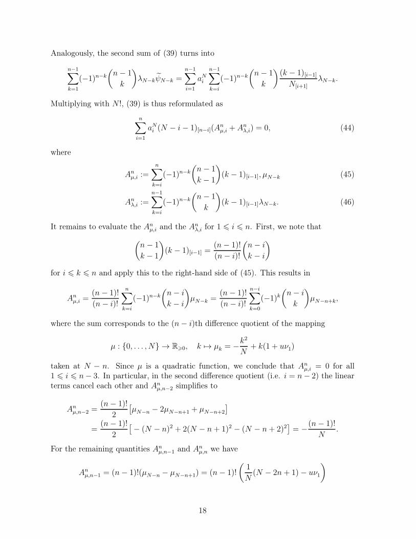
Analogously, the second sum of (39) turns into

n−1∑

k=1

(−1)n−k

(n− 1

k

)λN−kψ̃N−k =

n−1∑

i=1

aNi

n−1∑

k=i

(−1)n−k

(n− 1

k

)(k − 1)[i−1]

N[i+1]

λN−k.

Multiplying with N !, (39) is thus reformulated as

n∑

i=1

aNi (N − i− 1)[n−i](Anµ,i + An

λ,i) = 0, (44)

where

Anµ,i :=

n∑

k=i

(−1)n−k

(n− 1

k − 1

)(k − 1)[i−1], µN−k (45)

Anλ,i :=

n−1∑

k=i

(−1)n−k

(n− 1

k

)(k − 1)[i−1]λN−k. (46)

It remains to evaluate the Anµ,i and the An

λ,i for 1 6 i 6 n. First, we note that

(n− 1

k − 1

)(k − 1)[i−1] =

(n− 1)!

(n− i)!

(n− i

k − i

)

for i 6 k 6 n and apply this to the right-hand side of (45). This results in

Anµ,i =

(n− 1)!

(n− i)!

n∑

k=i

(−1)n−k

(n− i

k − i

)µN−k =

(n− 1)!

(n− i)!

n−i∑

k=0

(−1)k(n− i

k

)µN−n+k,

where the sum corresponds to the (n− i)th difference quotient of the mapping

µ : {0, . . . , N} → R>0, k 7→ µk = −k2

N+ k(1 + uν1)

taken at N − n. Since µ is a quadratic function, we conclude that Anµ,i = 0 for all

1 6 i 6 n− 3. In particular, in the second difference quotient (i.e. i = n− 2) the linearterms cancel each other and An

µ,n−2 simplifies to

Anµ,n−2 =

(n− 1)!

2

[µN−n − 2µN−n+1 + µN−n+2

]

=(n− 1)!

2

[− (N − n)2 + 2(N − n+ 1)2 − (N − n+ 2)2

]= −

(n− 1)!

N.

For the remaining quantities Anµ,n−1 and An

µ,n we have

Anµ,n−1 = (n− 1)!(µN−n − µN−n+1) = (n− 1)!

(1

N(N − 2n+ 1)− uν1

)

18

andAn

µ,n = (n− 1)!µN−n = (n− 1)!(N − n)( nN

+ uν1

).

We now calculate the Anλ,i. Since

(n− 1

k

)(k − 1)[i−1] =

1

k

(n− 1)!

(n− 1− i)!

(n− 1− i

k − i

)

for i 6 k 6 n− 1, we obtain that

Anλ,i =

(n− 1)!

(n− 1− i)!

n−1∑

k=i

(−1)n−k

(n− 1− i

k − i

)λN−k

k

=(n− 1)!

(n− 1− i)!

n−1−i∑

k=0

(−1)k+1

(n− 1− i

k

)λN−(n−1−k)

n− 1− k,

where the sum now coincides with the (n − 1 − i)th difference quotient of the affinefunction

λ : {0, . . . , N − 1} → R>0, k 7→λk

N − k=

k

N(1 + s) + uν0

taken at N − (n− 1). Consequently, Anλ,i = 0 for all 1 6 i 6 n− 3, and in An

λ,n−2 (moreprecisely in the first difference quotient of λ at N − (n− 1)) the constant terms canceleach other. Thus,

Anλ,n−2 = (n− 1)!

[−λN−(n−1)

n− 1+λN−(n−2)

n− 2

]

= (n− 1)!1 + s

N[N − (n− 2)− (N − (n− 1))] = (n− 1)!

1 + s

N

and so

Anλ,n−1 = −(n− 1)!

λN−(n−1)

n− 1= −(n− 1)!

[N − (n− 1)

N(1 + s) + uν0

].

Combining (44) with the results for Anµ,i and An

λ,i yields the assertion (42).

It will not come as a surprise now that the discrete recursions of the aNn obtained inThm. 2 lead to Fearnhead’s coefficients an in the limit N → ∞. According to Thm. 3 inthe Appendix, ψN

kNconverges to ψ(x) for any given sequence (kN)N∈N with 0 < kN < N

and limN→∞kNN

= x. Comparing (40) with (14), we obtain

limN→∞

aNn = an

for all n > 1. The recursions (15) of Fearnhead’s coefficients then follow directly fromthe recursions in Thm. 2 in the limit N → ∞.

19

6 Discussion

More than fifteen years after the discovery of the ancestral selection graph by Neuhauserand Krone [14, 16], ancestral processes with selection constitute an active area of re-search, see, e.g., the recent contributions [6, 7, 15, 18, 21]. Still, the ASG remains achallenge: Despite the elegance and intuitive appeal of the concept, it is difficult tohandle when it comes to concrete applications. Indeed, only very few properties ofgenealogical processes in mutation-selection balance could be described explicitly untiltoday (see the conditional ASG [22, 23] for an example). Even the special case of asingle ancestral line (emerging from a sample of size one) is not yet fully understood.The work by Fearnhead [9] and Taylor [20] established important results about the CAPwith the help of diffusion theory and analytical tools, but the particle representationcan only be partially recovered behind the continuous limit. In this article, we havetherefore made a first step towards complementing the picture by attacking the problemfrom the discrete (finite-population) side. Let us briefly summarise our results.

The pivotal quantity considered here is the fixation probability of the offspring of allfit individuals, regardless of the types of the offspring. Starting from the particle pictureand using elementary arguments of first-step analysis, we obtained a difference equationfor these fixation probabilities. In the limit N → ∞, the equation turns into the (second-order ODE) boundary problem obtained via diffusion theory by Taylor [20], but nowwith an intuitive interpretation attached to it.

We have given the solution of the difference equation in closed form; the resultingfixation probabilities provide a generalisation of the well-known finite-population fixationprobabilities in the case with selection only (note that they do not require the populationto be stationary). As a little detour, we also revisited the limiting continuous boundaryvalue problem and solved it via elementary methods, without the need of the seriesexpansion employed previously.

The fixation probabilities are intimately related with the stationary type distributionon the ancestral line and can thus be used for an alternative derivation of the recur-sions that characterise Fearnhead’s coefficients. Fearnhead obtained these recursionsby guessing and direct (but technical) verification of the stationarity condition; Taylorderived them in a constructive way by inserting the ansatz (16) into the boundary valueproblem (11) and performing a somewhat tedious differentiation exercise. Here we havetaken a third route that relies on the difference equation (25) and stays entirely withinthe discrete setting.

Altogether, the finite-population results contain more information than those obtainedwithin the diffusion limit; first, because they are not restricted to weak selection, andsecond, because they are more directly related to the underlying particle picture. Bothmotivations also underlie, for example, the recent work by Pokalyuk and Pfaffelhuber[18], who re-analysed the process of fixation under strong selection (in the absence ofmutation) with the help of an ASG in a discrete setting.

Clearly, the present article is only a first step towards a better understanding of theparticle picture related to the common ancestor process. It is known already that thecoefficients an may be interpreted as the probabilities that there are n virtual branches

20

in the pruned ASG at stationarity (see Section 3.2); but the genealogical content of therecursions (15) remains to be elucidated. It would also be desirable to generalise theresults to finite type spaces, in the spirit of Etheridge and Griffiths [6].

Acknowledgement

It is our pleasure to thank Anton Wakolbinger for enlightening discussions, and for Fig. 2.We are grateful to Jay Taylor for valuable comments on the manuscript. This projectreceived financial support by Deutsche Forschungsgemeinschaft (SPP 1590), grant no.BA2469/5-1.

Appendix

In Section 4.1 we have presented an alternative derivation of the boundary value problemfor the conditional probability h. It remains to prove that limN→∞ hNkN = h(x), with

x ∈ [0, 1], 0 < kN < N , limN→∞kNN

= x and h as given as in (7).Since hNk = k

N+ ψN

k and h(x) = x + ψ(x), respectively, it suffices to show the corre-sponding convergence of the ψN

k . For ease of exposition we assume here that the processis stationary.

Lemma 3. Let x̃ be as in (8). Then

limN→∞

NψNN−1 =

σ

1 + θν1(1− x̃).

Proof. Since the stationary distribution πNZ of

(ZN

t

)t>0

(cf. (2)) satisfies

n−1∏

i=1

λNiµNi

=πNZ (n)

CN

µNn

λN0, (47)

for 1 6 n 6 N , equation (30) leads to

NψNN−1 =

NsN1 +NuNν1

∑N

n=1 πNZ (N − n + 1)µN

N−n+1n−1N∑N

n=1 πNZ (N − n+ 1)µN

N−n+1

=NsN

1 +NuNν1

∑N

n=1 πNZ (n)µN

nN−nN∑N

n=1 πNZ (n)µN

n

=NsN

1 +NuNν1

∑N

n=1 πNZ (n)n(N−n)2

N3

(1 +

NuNν1

N−n

)

∑N

n=1 πNZ (n)n(N−n)

N2

(1 +

NuNν1

N−n

) ,

where we have used (1) in the last step. The stationary distribution of the rescaled pro-cess

(XN

t

)t>0

is given by(πNX

(iN

))06i6N

, where πNX

(iN

)= πN

Z (i). Besides, the sequence

21

of processes(XN

t

)t>0

converges to (Xt)t>0 in distribution, hence

limN→∞

NψNN−1 = lim

N→∞

NsN1 +NuNν1

EπN

X

(XN

(1−XN

)2 (1 +

uNν1

1−XN

))

EπN

X

(XN (1−XN)

(1 +

uNν1

1−XN

))

=σ

1 + θν1

EπX(X(1−X)2)

EπX(X(1−X))

=σ

1 + θν1(1− x̃),

as claimed.

Remark 2. The proof gives an alternative way to obtain the initial value a1 (cf. (18))of recursion (15).

Theorem 3. For a given x ∈ [0, 1], let (kN)N∈N be a sequence with 0 < kN < N and

limN→∞kNN

= x. Then

limN→∞

ψNkN

= ψ(x),

where ψ is the solution of the boundary value problem (11).

Proof. Using first Theorem 1, then (47), and finally (1), we obtain

ψNk =

k(N − k)

µNk

N−k∑

n=1

(N−n∏

i=k+1

λNiµNi

)(µNN−1

N − 1ψNN−1 −

sN(n− 1)

N2

)

=k(N − k)

µNk

(µNk+1π

NZ (k + 1)

)−1N−k−1∑

n=0

µNN−nπ

NZ (N − n)

(µNN−1

N − 1ψNN−1 −

sNn

N2

)

=

(1 +O

(1

N

))(k + 1

N

N − k − 1

NπNZ (k + 1)

)−1

×1

N

N−k−1∑

n=0

πNZ (N − n)

N − n

N

n

N

(1 +

NuNν1n

)((1 +NuNν1)Nψ

NN−1 −NsN

n

N

).

In order to analyse the convergence of this expression, define

SN1 (k) :=

k + 1

N

N − k − 1

NπNZ (k + 1),

SN2 (k) :=

1

N

N−k−1∑

n=0

πNZ (N − n)

N − n

N

n

N

((1 +NuNν1)Nψ

NN−1 −NsN

n

N

)

=

∫ 1

0

TNk (y)dy,

SN3 (k) :=

1

N

N−k−1∑

n=0

πNZ (N − n)

N − n

NuNν1

((1 +NuNν1)Nψ

NN−1 −NsN

n

N

)

=

∫ 1

0

T̃Nk (y)dy,

22

with step functions TNk : [0, 1] → R, T̃N

k : [0, 1] → R given by

TNk (y) :=

1{n6N−k−1}πNZ (N − n)N−n

NnN

((1 +NuNν1)Nψ

NN−1 −NsN

nN

),

if nN

6 y < n+1N, n ∈ {0, . . . , N − 1},

0, if y = 1,

T̃Nk (y) :=

1{n6N−k−1}πNZ (N − n)N−n

NuNν1

((1 +NuNν1)Nψ

NN−1 −NsN

nN

),

if nN

6 y < n+1N, n ∈ {0, . . . , N − 1},

0, if y = 1.

Consider now a sequence (kN)N∈N as in the assumptions. Then limN→∞ πNZ (kN) = πX(x)

(cf. [5, p. 319]), and due to Lemma 3

limN→∞

SN1 (kN) = x(1− x)πX(x),

limN→∞

TNkN

(kN) = 1{y61−x}πX(1− y)(1− y)y(σ(1− x̃)− σy),

limN→∞

T̃NkN

(kN) = 0.

Since TNk and T̃N

k are bounded, we have

limN→∞

SN2 (kN) =

∫ 1−x

0

πX(1− y)(1− y)y(σ(1− x̃)− σy)dy,

limN→∞

SN3 (kN) = 0,

thus

limN→∞

ψNkN

= (x(1− x)πX(x))−1

∫ 1−x

0

πX(1− y)(1− y)y(σ(1− x̃)− σy)dy.

Substituting on the right-hand side yields

limN→∞

ψNkN

= (x(1− x)πX(x))−1 σ

∫ 1

x

πX(y)y(1− y)(y − x̃)dy

= (x(1− x)πX(x))−1 σ

[∫ 1

0

πX(y)y(1− y)(y − x̃)dy +

∫ x

0

πX(y)y(1− y)(x̃− y)dy

]

= (x(1− x)πX(x))−1 σ

∫ x

0

πX(y)y(1− y)(x̃− y)dy = ψ(x),

where the second-last equality goes back to the definition of x̃ in (8), and the last is dueto (7), (10) and (2).

References

[1] E. Baake, R. Bialowons, Ancestral processes with selection: Branching and Moranmodels, Banach Center Publications 80 (2008), 33-52

23

[2] N. H. Barton, A. M. Etheridge, A. K. Sturm, Coalescence in a random back-ground, Ann. Appl. Prob. 14 (2004), 754-785

[3] G. Birkhoff, G. Rota, Ordinary differential equations, 2. ed., Xerox College Publ.,Lexington, Mass., 1969

[4] R. Durrett, Probability Models for DNA Sequence Evolution, Springer, New York,2002

[5] R. Durrett, Probability Models for DNA Sequence Evolution, 2. ed., Springer,New York, 2008

[6] A. M. Etheridge, R. C. Griffiths, A coalescent dual process in a Moran modelwith genic selection, Theor. Pop. Biol. 75 (2009), 320-330

[7] A. M. Etheridge, R. C. Griffiths, J. E. Taylor, A coalescent dual process in aMoran model with genic selection, and the Lambda coalescent limit, Theor. Pop.Biol. 78 (2010), 77-92

[8] W. J. Ewens, Mathematical Population Genetics. I. Theoretical Introduction, 2.ed., Springer, New York, 2004

[9] P. Fearnhead, The common ancestor at a nonneutral locus, J. Appl. Prob. 39(2002), 38-54

[10] L. R. Ford, Differential Equations, 2. ed., MacGraw-Hill, New York, 1955

[11] S. Karlin, H. M. Taylor, A Second Course in Stochastic Processes, AcademicPress, San Diego, 1981

[12] J. F. C. Kingman, The coalescent, Stoch. Proc. Appl. 13 (1982), 235-248

[13] J. F. C. Kingman, On the genealogy of large populations, J. Appl. Prob. 19A(1982), 27-43

[14] S. M. Krone, C. Neuhauser, Ancestral processes with selection, Theor. Pop. Biol.51 (1997), 210-237

[15] S. Mano, Duality, ancestral and diffusion processes in models with selection,Theor. Pop. Biol. 75 (2009), 164-175

[16] C. Neuhauser, S. M. Krone, The genealogy of samples in models with selection,Genetics 145 (1997), 519-534

[17] J. R. Norris, Markov Chains, Cambridge University Press, Cambridge, 1999

[18] C. Pokalyuk, P. Pfaffelhuber, The ancestral selection graph under strong direc-tional selection, Theor. Pop. Biol. (2012) (online first)

24

[19] M. Stephens, P. Donnelly, Ancestral inference in population genetics models withselection, Aust. N. Z. J. Stat. 45 (2003), 901-931

[20] J. E. Taylor, The common ancestor process for a Wright-Fisher diffusion, Elec-tron. J. Probab. 12 (2007), 808-847

[21] C. Vogl, F. Clemente, The allele-frequency spectrum in a decoupled Moran modelwith mutation, drift, and directional selection, assuming small mutation rates,Theor. Pop. Biol. 81 (2012), 197-209

[22] J. Wakeley, Conditional gene genealogies under strong purifying selection, Mol.Biol. Evol. 25 (2008), 2615-2626

[23] J. Wakeley, O. Sargsyan, The conditional ancestral selection graph with strongbalancing selection, Theor. Pop. Biol. 75 (2009), 355-364

25