the common cause principle - philsci-archivethe common cause principle explanation via screening o...
TRANSCRIPT

The Common Cause Principle
Explanation via screening o
Leszek Wro«ski
September 10, 2010
Ph.D. dissertation prepared under the supervision of
Prof. Tomasz Placek
Institute of Philosophy
Jagiellonian University
Kraków, Poland

Contents
1 Introduction 4
2 The Principle of the Common Cause: its shapes and content 7
2.1 Probability: the basics . . . . . . . . . . . . . . . . . . . . . . 7
2.1.1 Screening o . . . . . . . . . . . . . . . . . . . . . . . . 12
2.1.2 Observing probabilities and correlations . . . . . . . . 13
2.2 The plurality of the Principles . . . . . . . . . . . . . . . . . . 15
2.3 What Reichenbach wrote . . . . . . . . . . . . . . . . . . . . . 21
2.3.1 Reichenbach's argument for the Principle . . . . . . . . 27
2.3.2 Other problems with Reichenbach's approach . . . . . 31
2.4 The PCC after Reichenbach . . . . . . . . . . . . . . . . . . . 41
2.4.1 The argument from conservation principles . . . . . . . 43
2.4.2 The sea levels vs. bread prices argument . . . . . . . 44
2.4.3 Which correlations demand explanation? . . . . . . . . 47
2.5 An epistemic position . . . . . . . . . . . . . . . . . . . . . . . 51
3 Screening o and explanation: formal properties 52
3.1 The deductive explanatory feature . . . . . . . . . . . . . . . 57
3.2 In search for common causes, screening o is enough . . . . . 59
3.3 Common common constructs . . . . . . . . . . . . . . . . . . 62
3.4 Explanation via screenersthe general picture . . . . . . . . . 65
1
3.4.1 Weakening the screening o condition . . . . . . . . . . 66
3.4.2 Introducing deductive explanantes . . . . . . . . . . . . 69
4 The Principle of the Common Cause and the Bell inequali-
ties 73
4.1 The big space approach and the many spaces approach . . . . 75
4.2 Deriving the Bell inequalities . . . . . . . . . . . . . . . . . . . 77
4.3 The Bell inequalities via a non-empirical joint measure . . . . 79
4.4 A Bell-CH inequality from weakened assumptions . . . . . . . 82
4.5 Connection with the PCC . . . . . . . . . . . . . . . . . . . . 84
4.6 Separate common causescontra and pro . . . . . . . . . . . 90
4.7 Exploiting the detection loophole . . . . . . . . . . . . . . . . 94
4.8 Common causes as hypersurfaces . . . . . . . . . . . . . . . . 94
4.9 Summary . . . . . . . . . . . . . . . . . . . . . . . . . . . . . 95
5 The Principle of the Common Cause and the Causal Markov
Condition 97
5.1 DAGsan introduction . . . . . . . . . . . . . . . . . . . . . 99
5.2 The Causal Markov Condition . . . . . . . . . . . . . . . . . . 101
5.3 Conclusions . . . . . . . . . . . . . . . . . . . . . . . . . . . . 105
6 Causal closedness 107
6.0.1 A preliminary formal remark . . . . . . . . . . . . . . . 107
6.1 Causal (up-to-n-)closedness . . . . . . . . . . . . . . . . . . . 108
6.1.1 Introduction . . . . . . . . . . . . . . . . . . . . . . . . 108
6.1.2 Preliminary denitions . . . . . . . . . . . . . . . . . . 111
6.1.3 Summary of the results of this chapter . . . . . . . . . 113
6.2 Proofs . . . . . . . . . . . . . . . . . . . . . . . . . . . . . . . 114
6.2.1 Some useful parameters . . . . . . . . . . . . . . . . . 114
6.2.2 Proof of theorem 3 . . . . . . . . . . . . . . . . . . . . 115
2
6.2.3 Proofs of lemmas 9-11 . . . . . . . . . . . . . . . . . . 129
6.3 The proper / improper common cause distinction and the
relations of logical independence . . . . . . . . . . . . . . . . . 132
6.4 Other independence relations . . . . . . . . . . . . . . . . . . 134
6.5 A slight generalization . . . . . . . . . . . . . . . . . . . . . . 136
6.5.1 Examples . . . . . . . . . . . . . . . . . . . . . . . . . 138
6.6 Application for constructing Bayesian networksa negative
opinion . . . . . . . . . . . . . . . . . . . . . . . . . . . . . . . 139
6.7 The existence of deductive explanantes . . . . . . . . . . . . . 142
6.8 Conclusions and problems . . . . . . . . . . . . . . . . . . . . 144
6.9 Causal closedness of atomless spaces . . . . . . . . . . . . . . 145
7 Causal completability 147
7.1 Known results (the classical case) . . . . . . . . . . . . . . . . 148
7.2 Causal completability the easy waysplitting the atom . . . 149
7.3 Causal completability of classical probability spacesthe ge-
neral case . . . . . . . . . . . . . . . . . . . . . . . . . . . . . 151
7.4 Causal completability of non-classical probability spacessome
known results and prospects . . . . . . . . . . . . . . . . . . . 154
8 Statistical ε-common causes 157
8.1 Binomial distributions . . . . . . . . . . . . . . . . . . . . . . 160
8.2 A few contrastive examples . . . . . . . . . . . . . . . . . . . . 161
9 Conclusion 165
3

Chapter 1
Introduction
In one of its most basic and informal shapes, the principle of the common
cause states that any surprising correlation between two factors which are
believed not to directly inuence one another is due to their (possibly hidden)
common cause. In the history of philosophy it is easy to nd examples of
similar reasoning; one needs to look no further than the mind-body problem.
There is a truly astonishing correlation between our thoughts of the I want
to wave my hand sort and the movements of our hands of the waving sort.
A venerable solution to this quandary is that of invoking God as the common
cause (which was the road taken e.g. by Malebranche).
We can perhaps look for similar causal intuitions in Mill's System of Logic.
From the fth Canon of Induction it follows that a concomitant variation in
two phenomena of which none is a cause of the other is a sign of a connec-
tion between the two by some fact of causation. Mill begins his exposition
of the Canon by referring to the case in which this fact is the phenomena
being two eects of a common cause (Vol. I, Book III, Chapter VIII of Mill
(1868)). Bertrand Russell is on a similar track when he writes of identity
of structure leading to the assumption of a common causal origin (Rus-
sell (2009), p. 409). We, however, will be concerned with an idea which
4

possesses a probabilistic formulation. It was introduced, in the form of a
general principle, by Hans Reichenbach in his posthumously published book
The Direction of Time. The central notion of the principle in Reichenbach's
formulation, and of the current essay, is that of screening o: two correlated
events are screened o by a third event if conditioning on the third event
makes them probabilistically independent. Reichenbach's principle marks
also the beginning of a new eld of philosophy: namely, that of probabilistic
causality.
The main results of this work are presented in chapters 6 and 7. For the
most part, the current essay can be seen as an eort at checking how far one
can go with the purely statistical notions revolving around Reichenbach's
idea of common cause. In short, the answer is surprisingly far; in some
classes of probability spaces all correlations between interesting1 events
possess explanations of such sort. However, this fact lends itself to opposing
interpretations; more on that in the conclusion. Chapters 6 and 7 contain
mathematical results concerning these issues. The screening-o condition
requires an equality of a probabilistic nature to hold; chapter 8 is a short
discussion of slightly weakened versions of the condition, which hold if the
sides of the above mentioned equality dier to a small degree.
In chapter 2, after some mathematical preliminaries, we study the various
formulations of the principle which might be said to stem from the original
idea of Reichenbach. We also examine a few of the most salient counterar-
guments, which undermine at least some of the formulations. Chapter 3 is
of a formal nature, dealing with various probabilistic notions which can be
thought of as generalizations of Reichenbach's concept of common cause. The
next chapter concerns the relationship between the idea of common causal ex-
planation and the Bell inequalities. In chapter 5 we briey present the form
of Reichenbach's principle which can be found in the eld of representing
1 E.g. logically independent, this will be formally dened in chapter 6.
5
causal structures by means of directed acyclic graphs.
Acknowledgments
First and foremost, my thanks go to Professor Tomasz Placek, the best
Ph.D. supervisor in any bundle of branching space-times.
My interest in the subject sparked during the '08 Summer School in Pro-
babilistic Causality at the CEU University in Budapest. I would like to
thank Professor Miklós Rédei for introducing me to the problems discussed
in chapter 6.
I owe a great deal to Michaª Marczyk, with whom I extensively worked on
the issues of causal closedness of probability spaces. The material in sections
6.1-6.5 originates from our joint research; also, theorem 1 from chapter 3 is
our joint result.
I am grateful to the faculty and PhD students of the Epistemology De-
partment at the Institute of Philosophy of the Jagiellonian University for
insightful comments after my talks regarding the issues covered in this dis-
sertation. I would also like to thank Jakub Byszewski, Lech Duraj, Michaª
Skrzypczak, Michaª Staromiejski and Andrzej Wro«ski for helpful discussions
on mathematical topics.
6

Chapter 2
The Principle of the Common
Cause: its shapes and content
2.1 Probability: the basics
Before we state the various forms of the Principle, some of which will be of
a formal nature, a few denitions are in order.
Denition 1 [Probability space] A probability space is a triple 〈Ω,F , P 〉such that:
• Ω is a non-empty set;
• F is a nonempty family of subsets of Ω which is closed under comple-
ment and countable union;
• P is a function from F to [0, 1] ⊆ R such that
• P (Ω) = 1;
• P is countably additive: for a countable family G of pairwise dis-
joint members of F , P (∪G) =∑
A∈G P (A).
7

In the context of a probability space 〈Ω,F , P 〉, Ω is called the sample
space, F is called the event space, and P is called the probability function (or
measure). The members of F are called events.
The above denition captures the content of the concept of a classical
probability space. In one of the chapters to come we will also discuss non-
classical spaces, but let us postpone their denition till then. Also, in a
later chapter we will treat probability spaces as pairs consisting of a Boolean
algebra and a measure dened on it; this is because we will be speaking mostly
about nite structures for which any Boolean algebra of subsets is of course
complete with regard to the operations of complement and countable union
(and vice versa, any such family is a Boolean algebra). In general, though, it
may be that a Boolean algebra of subsets of a given set is incomplete w.r.t.
the operation of countable union.
The complement of an event A, F \ A, will be written as A⊥. If it is
evident from the context that A and B are events, we will sometimes write
P (AB) instead of P (A∧B) or P (A∩B) for the probability that both
A and B occur.
Every event B ∈ F such that P (B) 6= 0 determines a measure PB on the
same event space: namely, for any A ∈ F , PB(A) := P (AB)P (B)
. We dene the
conditional probability of A given B to be equal to PB(A); to refer to it, we
will almost exclusively use the traditional notation P (A | B). If P (B) = 0,
we take P (A | B) to be undened.
We will now dene the concept of a random variable. Our main reference
is Feller (1968), but the formulation of some denitions is inspired by Forster
(1988). Since in the sequel we do not use continuous random variables, we
can omit the usual measure-theoretic denitions; in fact, we will only need
random variables with a nite number of possible values. This is why by
random variable we will mean what is traditionally referred to as nite-
valued random variable.
8

Denition 2 [Random variable] Let 〈Ω,F , P 〉 be a probability space. LetV be a nite subset of R. A random variable on Ω is a function X : Ω→ V
such that
∀v ∈ V X−1(v) ∈ F .
If |V | = 2, X is called a binary random variable.
Thus every random variable determines a set of events directly tied to its
values. P (X = v), probability that the random variable X takes the value
v, is to be understood as P (X−1(v)); this is straightforwardly generalized
for any subset of V , so that for any V ′ ⊆ V , P (X ∈ V ′) =∑
v∈V ′ P (X = v).
Though random variables as dened above are real-valued functions, on
some occasions it might of course be useful to think of them as functions with
values of a dierent type, e.g. expressions yes or no. In numerical contexts
below we will always treat binary random variables as if they assume values
0 and 1.
It is immediate that a random variable X : Ω → V can be thought of
as a method of dividing the sample space Ω into at most |V | piecesthe
preimages of the members of V . There are two intuitive and important ways
of thinking about this, depending on our view of the sample space.
First, Ω can be considered to consist of all possible outcomes of an ex-
perimentfor example, if the experiment is a single toss of a six-sided die,
then Ω = 1, 2, 3, 4, 5, 6. A random variable may correspond to a feature
which some outcomes possess; for example, if X(1) = X(3) = X(5) = “yes”,
and X(2) = X(4) = X(6) = “no”, then the feature is being odd, and
P (X = “yes”) is to be interpreted as the probability that the outcome of
the toss is odd.
On the other hand, sometimes Ω is to be viewed not as a set of outcomes
of an experiment, but rather as the population on which an experiment is
conducted. Suppose a group of people is tested for a virus. Ω will then
9
consist of the test subjects, and P (X = “yes”) will mean the probability
that a randomly chosen test subject has the virus.
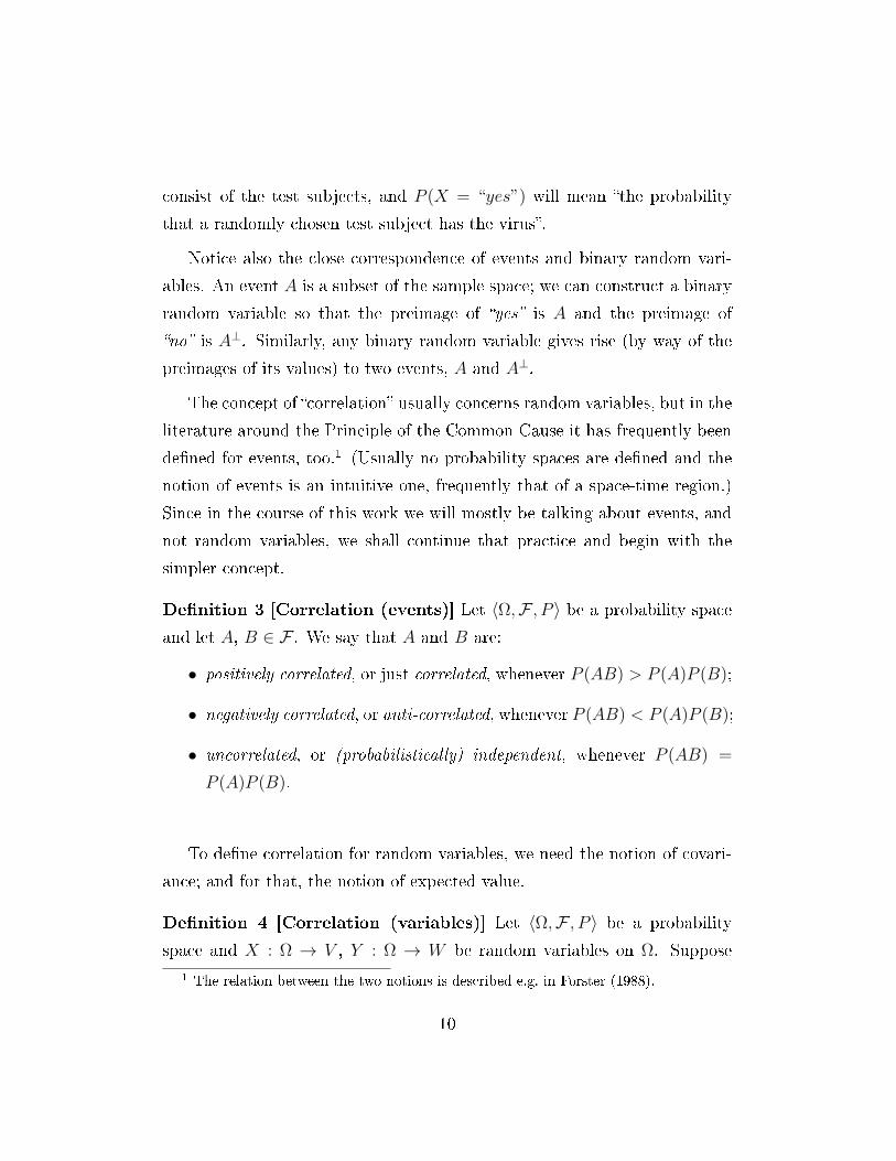
Notice also the close correspondence of events and binary random vari-
ables. An event A is a subset of the sample space; we can construct a binary
random variable so that the preimage of yes is A and the preimage of
no is A⊥. Similarly, any binary random variable gives rise (by way of the
preimages of its values) to two events, A and A⊥.
The concept of correlation usually concerns random variables, but in the
literature around the Principle of the Common Cause it has frequently been
dened for events, too.1 (Usually no probability spaces are dened and the
notion of events is an intuitive one, frequently that of a space-time region.)
Since in the course of this work we will mostly be talking about events, and
not random variables, we shall continue that practice and begin with the
simpler concept.
Denition 3 [Correlation (events)] Let 〈Ω,F , P 〉 be a probability space
and let A, B ∈ F . We say that A and B are:
• positively correlated, or just correlated, whenever P (AB) > P (A)P (B);
• negatively correlated, or anti-correlated, whenever P (AB) < P (A)P (B);
• uncorrelated, or (probabilistically) independent, whenever P (AB) =
P (A)P (B).
To dene correlation for random variables, we need the notion of covari-
ance; and for that, the notion of expected value.
Denition 4 [Correlation (variables)] Let 〈Ω,F , P 〉 be a probability
space and X : Ω → V , Y : Ω → W be random variables on Ω. Suppose
1 The relation between the two notions is described e.g. in Forster (1988).
10
X and Y have nite expectations. The correlation coecient of X and Y is
dened as
ρ(X, Y ) =Cov(X, Y )√
Cov(X,X) ·√Cov(Y, Y )
.
We will say the variables X and Y are correlated whenever ρ(X, Y ) > 0.
In the context of the Principle of the Common Cause, what demands
explanation is a correlation between events or a dependence between random
variables. As for the latter, some recent authors (e.g. Reiss (2007)) say
simply that Two variables X and Y are probabilistically dependent just in
case P (XY ) 6= P (X)P (Y ). Let us expand this into a denition.
Denition 5 [Dependence (variables)] Let 〈Ω,F , P 〉 be a probability
space and let X : Ω→ V and Y : Ω→ W be two random variables on Ω. X
and Y are dependent if
∃V ′ ⊆ V ∃W ′ ⊆ W : P (X ∈ V ′ ∧ Y ∈ W ′) 6= P (X ∈ V ′)P (Y ∈ W ′).
Note that for random variables the concepts of independence and noncor-
relation diverge. If two variables are independent, their correlation coecient
is 0, but not always vice versa; for examples see Feller (1968), p. 236. Still,
to restate the above, a non-zero correlation coecient means the variables
are dependent.
For binary variables X and Y their covariance is obviously equal to
P (X = 1 ∧ Y = 1)− P (X = 1)P (Y = 1).
This explains why the denition 3 can be seen as a special case of the de-
nition 4; events are correlated whenever their corresponding binary variables
are and vice versa.
11

2.1.1 Screening o
Perhaps the most important notion concerning the idea of common causes is
one of screening o.
Denition 6 [Screening o] Assume a probability space 〈Ω,F , P 〉 is given.Let A,B ∈ F . An event C is said to be a screener-o for the pair A,B if
P (AB | C) = P (A | C)P (B | C). (2.1)
In the case where A and B are correlated we also say that C screens o the
correlation.
If C is a screener-o for A,B, we will also frequently say that C screens
o A from B and vice versa. Another way of putting the fact is saying that
C renders A and B conditionally probabilistically independent. Observe that
the screening o condition 2.1 is equivalent to the following:
P (A | BC) = P (A | C) (2.2)
provided all probabilities are dened.
Denition 7 [Statistical relevance] Let 〈Ω,F , P 〉 be a probability space.
Let A,B ∈ F . We say that an event C ∈ F is positively statistically rele-
vant for A if P (A|C) > P (A|C⊥). We say that a family of events Ci isstatistically relevant for A and B if, whenever i 6= j,
(P (A | Ci)− P (A | Cj)
)(P (B | Ci)− P (B | Cj)
)> 0.
Notice that P (A|C) > P (A|C⊥) is equivalent to P (A|C) > P (A), if all
the probabilities are dened.
12

2.1.2 Observing probabilities and correlations
We now have the requisite denitions of probability and related concepts.
But how do we observe probabilities in the world? If probabilities are to
be limiting frequencies, as one notable interpretation would have it, then
we have a problem, since, as beings capable of nitely many operations, we
naturally observe only relative frequencies in nite samples. We can only pose
hypotheses about probabilitiesbut these hypotheses may be well-grounded,
thanks to the law of large numbers (see e.g. Feller (1968), p. 243).
If a probability of our experiment ending with a particular outcome is φ,
the more we repeat the experiment, the closer should the observed relative
frequency of the outcome come to φ. If the probability is unknown, the
question regarding the number of repetitions needing to be conducted for us
to be able to oer a reliable hypothesis regarding it is subtle, and the answer
to it depends on how reliable we require the hypothesis to be. These issues
are treated extensively e.g. in Blalock (1979). The technical details will not
be of interest to us; the important thing is that no reliable information about
probabilities of particular events (and so, a fortiori, about their correlation,
as well as probability distributions and correlation of random variables) can
be gathered from a small experimental sample.
It will be worthwhile to reiterate this point in an analysis of single oc-
currences of events which we nd unexpected or surprising. Suppose, for
instance, that someone rolled two fair six-sided dice on a at table and ended
up with two sixes. Why are we (a bit) surprised? Is the result improbable?
That particular combination (a six on the rst die, a six on the second die)
is improbable to exactly the same degree (1/36) as any other possible com-
bination; so the reason for the surprise must be something dierent. And
perhaps it is two-fold:
1. the sum of the results (12) is maximally dierent from the expected
13
value (7); and perhaps we implicitly compare the probability of rolling
it (1/36) with the probability of rolling 11 or more (1/12), 10 or more
(1/6) or more and so on;
2. all throws end up with the same score, which is quite an improbable
event (1/6) compared to the alternative, which we implicitly expect to
occur.
IfXi is the event die number i ends up with a 6, then P (X1X2) = 136; but
just from the occurrence of that particular event we by no means infer that
P (X1X2) > P (X1)P (X2). The reason for the fact that a single occurrence
of an improbable coincidence, being a conjunction of other events, startles
us, is not that we perceive it as evidence of a yet unsuspected correlation.
Otherwise we would always have to accuse lucky dice players, or have pity
on unlucky ones, for playing with unfair dice.
This is not to say that a proponent of the frequentist interpretation of
probability necessary cannot speak in any way about probabilities of sin-
gle events. Reichenbach himself would be an example to the contraryhis
way of ascribing probabilities to single events is described in section 72 of
Reichenbach (1949). Even though he states on p. 375 that single-case prob-
ability is a pseudo-concept, he develops a way of thinking about the single
case as the limit of the [reference] classes becoming gradually narrower and
narrower (ibid.). However, on his account single-case probabilities are, in
contrast to regular probabilities, dependent on the state of our knowledge;
and on the whole, he regards the statement about the probability of the
single case, not as having a meaning of its own, but as an elliptic mode of
speech (ibid., p. 376-377). Anyway, a frequentist should not in general let a
single occurrence of an event inuence his beliefs regarding the probabilities
inherent in a given situation.
A dierent issue is whether the data we are analyzing originates from any
14

sort of probabilistic set-up; whether it is appropriate to consider any under-
lying probabilities at all. If e.g. some parts of the experiment are inuenced
by human choice, is it wise to consider the probability of a person choosing
a particular option? Cartwright (1999) holds the view that no statements
regarding probabilities in the world are true simpliciter, but in fact may only
be true ceteris paribus ; they need to arise in the context of a probability
machine, a xed arrangement of components with stable capacities giving
rise to regular behaviour.
We can make sense of the probability of drawing two red balls in
a row from an urn of a certain composition with replacement; but
we cannot make sense of the probability of six percent ination
in the United Kingdom next year without an implicit reference to
a specic social and institutional structure that will serve as the
chance set-up that generates this probability (Cartwright (1999),
p. 175).2
The chance set-ups may be of various kinds: the stochastic process is
the world line of the persisting object (a die, a socio-economic structure)
(Reiss (2007), emphasis ours). With no additional information, though, it is
unwise to expect a set of data, and the derived relative frequencies of events
as indicative of probability.
2.2 The plurality of the Principles
The literature on the Principle (henceforth referred to as PCC) abounds
in dissenting opinions regarding its validity. It is false (Arntzenius (1992)).
It is non-falsiable (Hofer-Szabó, Rédei & Szabó (2000)). It is a fallible
2 Chapter 7.4 of Cartwright's book contains a detailed description of a probability
machine in the context of probabilistic claims about causality made by Salmon (1971).
15

epistemic principle (Reiss (2007)). Lastly, it is derivable from the second
law of thermodynamics3 (Reichenbach (1971)). Since each of the above is
well-argued for, and since there is such a plethora of views on the subject, the
subject clearly must be something dierent in every case. The principle some
authors are arguing against is not always the same principle their opponents
promote.
The multiplicity of forms of the PCC has already been discussed in the
literature in e.g. Berkovitz (2000) and sections 3.4 − 3.5 of Placek (2000),
but we shall initially take an approach dierent from those displayed by
these texts. Berkovitz analyzes how the prospects of the principle depend
on which concepts of correlation (between types or tokens) and causation
are employed. Placek dierentiates various versions of the principle on the
basis of the mathematical constitution of the common causewhether it is
a single event or an n-tuple of eventsand whether it is to explain a single
correlation or more. While we will also discuss these important matters later
on, right now we propose to consider a gradual process of infusing an initially
sketchy and informal principle with formal content.
Throughout the process we will move from purely informal principles to
purely formal ones. The former may arouse deep intuitions and interesting,
yet usually inconclusive discussions; the latter can be formally proved or
disproved, but one may doubt their relevance to philosophy, or, in the case
an antipathy to all things formal is displayed, to anything interesting at all.
This is perhaps the usual case when philosophy meets mathematics: the
more formal your considerations, the bigger risk of losing track of signicant
philosophical content. That said, I have a predilection for formal philosophy,
which will perhaps be mostly visible in chapter 6; I nd it heartening for
a philosopher to be able to prove something from time to time. It would
be ideal if an interesting and sound philosophical argumentation could be at
3 Admittedly, only with an additional assumption. See section 2.3.1.
16

least partly based on mathematical proofs.
A side-note: probability is a relatively new tool for philosophy. Perhaps
a big role in its introduction to philosophy was played by Hans Reichen-
bach's 1956 book The Direction of Time (to which we refer throughout this
essay as Reichenbach (1971)), where the PCC was rst formulated. Sub-
sequently probability has been widely used by researchers in the eld of so
called probabilistic causality. To this day, most philosophers writing about
probability usually simply use expressions like P(A) in contexts in which
they would normally say the probability that A occurs, without dening
any probability spaces. This has the drawback that the notion of event is
foggy. The reader cannot be sure what qualies as an event and what does
not; he is expected to rely on his intuitions. We will see an example where
this can result an in unfortunate misunderstanding (see p. 39). I believe that
philosophy would benet if every author explicitly dened their probability
spaces, at the cost of their texts becoming perhaps a bit more dry and the
process of writing them getting more unwieldy.
We will not cite any proponents of the principles listed below, because it
seems almost every participant in the discussion uses a principle which is in
at least one small respect dierent from most of the others.
PCC 1 Suppose there is a correlation between two events, which are not
directly causally related. Then there exists a common cause of the correlated
events.
Notice that no views on the nature of causality are included in the above
formulation. While it is dicult to nd authors who would openly advocate
this view, some arguments oered against the PCC (or Reichenbach's
PCC)most notably Sober-style examples we will discuss in section 2.4.2
actually negate PCC 1, since the probabilistic description of the allegedly
existing common cause is largely irrelevant to the argument.
17

PCC 2 Some correlations demand explanation. Of these, some demand
explanation by means of a common cause. In each such case there exists
a common cause of the correlated events, which renders them conditionally
probabilistically independent.
There are two additions in comparison to PCC 1: rst (twofold), a quali-
cation is added that perhaps only some (not all) correlations stand in need
of common causal explanation; some authors use the word improbable to
describe them. Second, a probabilistic ingredient is added: the postulated
common cause of the correlated events should screen them o.
PCC 3 Let 〈Ω,F , P 〉 be a probability space. For any A, B ∈ F (such that
〈A,B〉 belongs to a relation of independence Lind), if P (AB) > P (A)P (B),
then there exists an event C ∈ F (dierent from both A and B) such that
P (AB | C) = P (A | C)P (B | C);
P (AB | C⊥) = P (A | C⊥)P (B | C⊥);
P (A | C) > P (A | C⊥);
P (B | C) > P (B | C⊥).
This version of the principle is of a formal nature. The word cause is
nowhere to be seen; it can be of course introduced, by dening a common
cause for A and B as an event meeting the four requirements above. (We
assume this denition for the remainder of this section.) PCC 3 is actually
meant to possess two variants: with or without the rst expression in paren-
theses. Frequently a relation of independence is introduced; it is usually at
least logical independence (so that e.g. the correlation between heads up
and tails down will not stand in need of an explanation in terms of a com-
mon cause), and perhaps ideally it is supposed also to cover direct causal
18

independence. However, if Lind is just logical independence, then PCC 3 is
simply false, as it is easy to nd examples of spaces with correlations between
logically independent events, for which no event meeting the requirements
above exists (see e.g. Hofer-Szabó, Rédei & Szabó (2000), p. 91). It is also
highly unlikely that xing the relation of independence so that it includes
less pairs than the relation of purely logical independence will alleviate this
diculty and make the principle generally plausible. However, an interesting
question is: in which classes of probability spaces and for which relations of
independence does the principle hold? We will discuss these issues at length
in chapter 6.
To state the last form of the principle we need to dene extension of
probability spaces.
Denition 8 [Extension] Let A = 〈Ω,F , P 〉, be a probability space. A
space A′ = 〈Ω′,F ′, P ′〉 is called an extension of A if there is a Boolean
algebra embedding h : F → F ′ which preserves the measure, that is, ∀A ∈F , P ′(h(A)) = P (A).
PCC 4 Let A = 〈Ω,F , P 〉 be a probability space. Suppose that A, B ∈ F(such that 〈A,B〉 belongs to a relation of independence Lind) are correlated,
but there exists no C ∈ F (dierent from both A and B) such that
P (AB | C) = P (A | C)P (B | C);
P (AB | C⊥) = P (A | C⊥)P (B | C⊥);
P (A | C) > P (A | C⊥);
P (B | C) > P (B | C⊥).
Then there exists a space A′ = 〈Ω′,F ′, P ′〉 such that A′ is an extension of A
by means of a homomorphism h and there exists an event C ′ ∈ F ′ such that
19

P ′(h(A)h(B) | C ′) = P ′(h(A) | C ′)P ′(h(B) | C ′);
P ′(h(A)h(B) | C ′⊥) = P ′(h(A) | C ′⊥)P ′(h(B) | C ′⊥);
P ′(h(A) | C ′) > P ′(h(A) | C ′⊥);
P ′(h(B) | C ′) > P ′(h(B) | C ′⊥).
As we have already said, there are numerous counterexamples to PCC 3,
which is a statement postulating, for each correlation in a given space, a
common cause in the same space. PCC 4 is, however, more subtle. Sup-
pose we observe an unexpected correlation during an experiment, but the
probability space we have chosen to operate within lacks common causes for
the correlated events. But perhaps the choice of the space was unfortunate;
perhaps we have not taken some factors into account and a dierent, more
ne-grained space, compatible with the observations to the same extent
as the original one, provides an explanation for the correlation in terms of
a common cause? In other words, can the original space be extended to a
space possessing a common cause for the yet unexplained correlation? And
in general, is it possible to extend a given probability space to one containing
common causes for all correlations? Perhaps surprisingly, the answer to both
questions is yes. We will deal with these matters extensively in chapter 7.
We have already mentioned that the place in which the PCC was intro-
duced was Reichenbach's Direction of Time. Subsequently, regardless of the
version of the principle they are concerned with, many authors credit Re-
ichenbach with the original idea. Some of them (e.g. Hoover (2003), p. 527)
content themselves with the following quotation: If an improbable coinci-
dence has occurred, there must exist a common cause4. In the next section
4Reichenbach (1971), p. 157.
20

we will try to convince the reader that such a selective quotation misses a
few important facets of Reichenbach's view of the Principle.
2.3 What Reichenbach wrote
Reichenbach's 1956 book is frequently taken to contain an important meta-
physical view of probabilistic causality (see e.g. Williamson (2009)). The
main object of the book, however, is to analyze the possibilities of den-
ing time direction by means of causal relations. Part IV discusses the case
of macrostatistics and it is there, in chapter 19, where the Principle of the
Common Cause originally appears.
Throughout his book Reichenbach frequently writes about probability
(his formulas will be put here in modern notation), however he did not choose
to adopt the Kolmogorovian concepts of event space and probability space,
which were then slowly gaining recognition. The choice was undoubtedly
motivated by the fact that he already had his own von Mises-style theory
of probability, developed earlier in Reichenbach (1949) (originally issued in
German in 1935). It is important to note at the beginning of this section
that, for Reichenbach, the term probability is always assumed to mean
the limit of a relative frequency (Reichenbach (1971), p. 123). Therefore
the question of probability of an event regarded in isolation of any sequence
of its possible occurrences or non-occurrences should be meaningless. To use
a popular philosophical term, for Reichenbach there should be no such things
as single-case probabilities.
The guiding idea behind Reichenbach's principle, and the source of
as we will seean important argument for one of Reichenbach's theses is
that the improbable should be explained in terms of causes, not in terms
of eects (Reichenbach (1971), p. 157); the short version of the Principle of
the Common Cause quoted at the end of the previous section comes right at
21

the end of the same paragraph. Let us quote the rst examples with which
Reichenbach's illustrates his principle (all quotes from ibid., p. 157):
• Suppose that lightning starts a brush re, and that a strong wind
blows and spreads the re, which is thus turned into a major disaster.
The coincidence of re and wind has here a common eect, the burning
over of a wide area. But when we ask why this coincidence occurred,
we do not refer to the common eect, but look for a common cause.
The thunderstorm that produced the lightning also produced the wind,
and the improbable coincidence is thus explained.
• Suppose both lamps in a room go out suddenly. We regard it as
improbable that by chance both bulbs burned out at the same time, and
look for a burned-out fuse or some other interruption of the common
power supply. The improbable coincidence is thus explained as the
product of a common cause.
• Or suppose several actors in a stage play fall ill, showing symptoms of
food poisoning. We assume that the poisoned food stems from the same
sourcefor instance, that it was contained in a common mealand
thus look for an explanation of the coincidence in terms of a common
cause.
Keeping in mind the concept of probability quoted above, up to this point
it would hardly seem surprising that the principle
Reichenbach's PCCthe coincidence formulation: If an im-
probable coincidence has occurred, there must exist a common cause
makes no mention of probability save for the word improbable in the
antecedent. Reichenbach quickly injects his principle with more probabilistic
content, though. First, he admits that chance coincidences, of course, are
22

not impossible, since the bulbs may simply burn out at the same moment
etc. Therefore, in such cases the existence of a common cause is not abso-
lutely certain, but only probable (ibid., emphasis mine), with the probability
increasing with the number of repeated coincidences. (Let us just note that
the concept of probability implicit here seems to be decidedly epistemicthe
more repeated coincidences we observe, the more strongly we should believe
in the existence of a common causeand thus hard to reconcile with the
earlier denition.) The author oers another two examples supporting the
principle (ibid., p. 158):
• Suppose two geysers which are not far apart spout irregularly, but
throw up their columns of water always at the same time. The exis-
tence of a subterranean connection of the two geysers with a common
reservoir of hot water is then practically certain.
• The fact that measuring instruments such as barometers always show
the same indication if they are not too far apart, is a consequence of
the existence of a common causehere, the air pressure.
We are then advised to treat the principle of the common cause as a
statistical problem (ibid.). In Reichenbach's view this means that we should
assume events A and B have been observed to occur frequently, which en-
ables us to consider probabilities P (A), P (B) and P (AB). The relationship
between two (improbably) simultaneously occurring events and both their
common cause and eect is depicted in terms of forks seen in gure 2.1.
Reichenbach claims the forks depict statistical relationships between the
events. However, in his examples cited above there always is some physical
process behind each arrow on the diagram.
The coincidence of events A and B has, for Reichenbach, a probability
exceeding that of a chance coincidence (ibid., p. 159) precisely when the
two events are correlated in terms of our denition 3. Suppose, then, the
23

Figure 2.1: A double fork, a fork open towards the future, a fork open towards
the past (from Reichenbach (1971)).
events are correlated. We assume that there exists a common cause C. If
there is more than one possible kind of common cause, C may represent the
disjunction of these causes (ibid.). An important assumption is now that
the fork ACB satises exactly the statistical requirements listed above in the
formulation of PCC 3:
P (AB | C) = P (A | C)P (B | C); (2.3)
P (AB | C⊥) = P (A | C⊥)P (B | C⊥); (2.4)
P (A | C) > P (A | C⊥); (2.5)
P (B | C) > P (B | C⊥). (2.6)
Namely, both C and C⊥ should screen o A from B, and C should be
statistically relevant both for A and B.
Reichenbach proceeds to point out two explanatory features of the pro-
posed common causes. The rst one is that from the conditions 2.3-2.6 the
correlation between A and B is deducible. (We shall investigate this and
24
related ideas in section 3.1.) This fact is interpreted by Reichenbach as
meaning that the fork ACB makes the conjunction of the two events A and
B more frequent than it would be for independent events (ibid.), and that
is why the author proposes to call such forks conjunctive forks. The second
explanatory feature of common causes is that, due to screening-o, the cor-
relation in a sense disappearsrelative to the cause C the events A and
B are mutually independent (ibid.). Due to these features, a common cause
makes it possible to derive statistical dependence from an independence. The
common cause is therefore the connecting link, and the conjunctive fork is
therefore the statistical model of the relationship formulated in the principle
of the common cause (ibid., p. 160).
What follows next is the proof of the above mentioned fact that from
conditions 2.3-2.6 one can derive the correlation between A and B. It is
thus quite puzzling why, on the next page (163), Reichenbach writes These
results may be summarized in terms of the principle of the common cause
(...). Which results? So far, the existence of common causes as the middle
links in conjunctive forks was distinctively assumed, not reached as any sort
of result. What is more important now, though, since the author attempts a
justication of the principle later on, is its formulation (reworded so it would
not refer to equations in Reichenbach's text by their numbers):
Reichenbach's PCCthe correlation formulation: If coinci-
dences of two events A and B occur more frequently than would correspond
to their independent occurrence, that is, if the events are correlated, then
there exists a common cause C for these events such that the fork ACB is
conjunctive.
Notice that with the move from speaking about single coincidences to
correlations the word improbable disappears. In the above formulation
there is no division between probable and improbable (or unexpected /
25

accidental) correlations. Common causes are to exist for all correlations.
What is, for Reichenbach, the relationship between the statistical condi-
tions 2.3-2.6 and the concept of common cause? Being a common cause of
A and B is not sucient for being the middle link of a conjunctive fork: A
and B may simply not be correlated (Reichenbach's example is that of two
dice being thrown by the same hand). In the other direction, being the mid-
dle element of a conjunctive fork is for Reichenbach certainly not sucient
for being a common cause, since common eects may also satisfy conditions
2.3-2.6. However, for his idea for dening time direction to work, it is ab-
solutely crucial to ascertain that if a conjunctive fork ACB is open5, then
C is a common cause of A and B and not their eect. This way he will be
able to frame his denition of time direction in terms of macrostatistics as
In a conjunctive fork ACB which is open on one side, C is earlier than A or
B (ibid., p. 162). But does he succeed in showing the causal asymmetry of
conjunctive forks? This may initially seem to be a side issue for the principle
of the common cause, but it is not: an example of a conjunctive fork open to
one side, containing two events and their common eect, such that there is
no common cause for the two events which together with them constitutes a
conjunctive fork, would be a counterexample to the principle. The fact that
the issue was discussed in this context by perhaps the staunchest proponent
of the principle, Wesley Salmon (1984), is another reason for which we will
return to it in one of the coming sections.
5 This seems to mean that one of the two possibilities (one of which is almost imme-
diately excluded) occurs: either (1) C is a common cause of A and B, and there exists no
common eect D of A and B such that ADB would constitute a conjunctive fork, or (2)
C is a common eect of A and B, and there exists no common cause D of A and B such
that ADB would constitute a conjunctive fork.
26
2.3.1 Reichenbach's argument for the Principle
What is, then, the justication given by Reichenbach for his principle? It
is supposed to follow from the second law of thermodynamicsthe entropy of
an isolated system which is not in equilibrium tends to increasesupplemented
with an additional assumption, labeled branch hypothesis, which we shall
now consider.
As we said earlier, in his book Reichenbach does not use the formalism of
probability spaces which has since then become the standard approach. In-
stead in 12 he introduces the so called Probability Lattice. In the context
of the book, it is a mathematical construction for describing processes of mix-
ture. A probability lattice is a two-dimensional matrix; each row represents
the history of a single object, e.g. a molecule of gas (thus it is also called a
time ensemble), and each column is a time-slice through the system under
consideration, containing information about the state of all molecules in the
system at a given time (being thus also called a space ensemble). To use
Reichenbach's own example, consider a container with two compartmentsL
and Rand assume there are molecules of nitrogen in compartment L and
oxygen in compartment R. Suppose the wall dividing the compartments is
removed and the substances begin to mix with each other. If we restrict our
attention to nitrogen only, and record only the positions of the molecules (in
a binary way, L or R), the rst column of our probability lattice should
be lled exclusively with Ls, while the farther we go to the right, the more
the proportion of Ls and Rs in a given column approaches 1/2.
The lattice will be a lattice of mixture (Reichenbach (1971), p. 103) only
if it meets a few conditions, discussed on pages 100-103 of the book. The
two simple ones regard the initial column (which should be ordered6) and
6 In the sense that it should illustrate a state of order; just like in the previous example,
the initialorderedstate of the system is illustrated by a column with the letter L in
all entries.
27

aftereect in rows (an R at position i in a row increases the chance for an R at
position i+1 in the same row). The other two, though, independence of the
rows and (especially) lattice invariance (which allows making inferences
from the time ensemble to the space ensemble), are highly non-trivial. It
would not be proper to study the conditions here in detail, since they are
not at the heart of Reichenbach's argument for the PCC.7
The formalism was needed because the branch hypothesis itself refers to a
lattice of mixture (Reichenbach (1971), p. 156). The general idea is that the
whole universe, as a whole, is a system the entropy of which is currently low,
but increases over time (barring some short-term anomalies). From the main
system smaller systems branch o, and are isolated for a certain periodbut
they are connected with the main system at both ends. The entropy of these
branch systems is also (in general) low at one of these points and high at
the other; the crucial thing is that the direction towards higher entropy is in
general parallel throughout the branch systems. This covers four out of ve
assumptions making up the hypothesis; the remaining one is that the lattice
of branch systems is a lattice of mixture.
Suppose, for now, the branch hypothesis is true. How should the PCC
follow? Reichenbach tries to shows rst (pp. 164-165) that if an ensemble of
branch systems is considered which contains two types of systems TA and TB
(the systems of the rst type may assume state A and the others state B)
7 But it has to be noted that while there may be some intuitive appeal of those two
conditions being connected with a mixing process, the author himself struggles with his
own notation, being forced to use sub-subscripts, and we hope the reader who consults
the book will agree that it is not evident that Reichenbach's formulas in his lattice-lingo
adequately express what he says in English. (For example, why does the right-hand side of
formula (17) (p. 101) express any vertical probability (as dened on p. 99) at all?) Even
if these diculties were dispensed with, there is no justication for lattice invariance save
for a reference to Reichenbach (1949), where (p. 174) it is stated that the kinetic theory
of gases makes a similar assumption.
28

such that sometimes a system of type TA and another of type TB coincide in
their rst state (call it C), and a composite probability lattice is constructed
from the two lattices for two system types by appropriately gluing some
rows on top of others so that for any case of the above mentioned coincidence
the row for the system of type TA is on top of the row for the system of type
TB, then the composite lattice satises the conditions for a conjunctive form
transcribed into Reichenbach's lattice notation. For future reference, let us
state that his goal here was to ascertain that whenever two causal lines
leading to A and B are connected by their rst element C, the fork ACB is
conjunctive (*).
Then Reichenbach claims that the branch hypothesis tells us that if a
state occurs more frequently in the space ensemble than corresponds to a
certain standard, namely, to its probability in the time ensemble, there must
have existed an interaction state in the past (p. 166) (**). This sentence
is dicult to grasp due to its lack of quantiers over columns and rows.
Should we read it as the branch hypothesis tells us that if in a lattice of
mixture there exist row k and column i such that a certain state occurs more
frequently in k than in i, (...) or the branch hypothesis tells us that if
in a given lattice of mixture it is true that for any row k and column i a
certain state occurs more frequently in k than in i, (...)? The fact that
in the previous paragraph we seem to have been actually considering three-
dimensional probability lattices8 does not help, either.
But let us, again, drop this issue (and the issue of whether the above
actually follows from the branch hypothesis). The next step in Reichenbach's
8 The additional dimension, apart from rows and columns, stems from the fact that
rows from the lattice for systems of type TA are above the ones for systems of type TB ; it
cannot be the two-dimensional sort of above used in statements like on this very page,
the previous line is above this one, since were it so, it wouldn't be possible for As and
Bs to happen in the same row of the composite lattice, which is explicitly required by
Reichenbach's mathematical formulas.
29

reasoning is that
If the two causal lines leading to A and B were not connected by
their rst elements, the probability of the joint occurrence would
be given by P (A) · P (B).9 (***)
This, unfortunately, begs the question. By contraposition and combi-
nation with (*) we get: if A and B are correlated or anti-correlated, the
two causal lines leading to A and B are connected by their rst element C,
and the fork ACB is conjunctive , which is at rst sight an even stronger
statement than the PCC.10 Statement (***) needs to be backed up, but is
not. It cannot be backed up by (**)because, however we understand it, it
is an implication from the fact that the probability of a given state in the
space ensemble is dierent (higher) from its probability in the time ensemble,
without reference to the actual values of the probabilities! So, a priori, it is
consistent with (**) that for some A and B, the causal lines leading to A
and B are not connected by their rst elements, but the probability of the
joint occurrence is given by P (A) · P (B) + 0.05, which is inconsistent with
(***).11 Sadly, we have to conclude that the argument given by Reichenbach
misses a link without which part (***) assumes the thesis. Thus the status
9 ibid.10 Only at rst sight, because if events A and B are anti-correlated, then A and B⊥
are positively correlated (and vice versa), so the PCC may also be read as demanding
explanation for anti-correlations.11 The point will be perhaps more palatable if made colloquially: everyone remembers
that correlation does not mean causation. But (since A and B, belonging by assumption
to isolated branch systems, cannot cause one another) (***) says basically that absence of
causation means absence of correlation! The author, when claiming (***), has to have in
mind something similar to the negation of the hackneyed slogan; namely, that correlation
does mean causation, if not between the correlated events (since they occur at the same
time or belong two isolated systems), but between them and their common cause. This is
a yet another informal statement of Reichenbach's PCC.
30

of the principle of the common cause in The Direction of Time is still that
of a hypothesis. It does not change the fact that it may well be a valuable
rule of human reasoning; simply, Reichenbach does not succeed in showing
it to be a well-proved theorem.
It has to be added that Reichenbach himself thought that the PCC reit-
erates the very principle which expresses the nucleus of the hypothesis of the
branch structure (ibid., p. 167). Perhaps, then, no separate argument for
PCC is needed and a justication of the hypothesis of the branch structure
would suce. We will argue that this prospect is sadly also not hopeful in
the next section, among a few other drawbacks of Reichenbach's account.
2.3.2 Other problems with Reichenbach's approach
The hypothesis of the branch structure: main system and entropy
The rst worry regarding the hypothesis concerns what it is that is supposed
to branch. Reichenbach oers a few illustrations. In the rst one (gure 2.2)
we are supposed to see a long upgrade of the entropy curve of the universe
and systems branching o from this upgrade, assuming that these branch
systems remain isolated for an innite time (ibid., p. 118). The second one
(gure 2.3) diers in that the systems which branch o from the main system
return to it and that it contains also a downgrade of the entropy curve.
In both images the vertical axis is supposed to depict entropy. And the
problem is that, while not all concepts of entropy are that of an additive
quality (see e.g. Palm (1978)), the types of entropy considered by Reichen-
bach are additive, as he says himself on p. 53 (If two systems are brought
together, their entropies are additive). Therefore, suppose the universe con-
sisted of a system which from time to time divides into two systems that
remain isolated for a certain period and then connect again. Since entropy is
additive, the initial part of the curve depicted in gure 2.3 should rather look
31
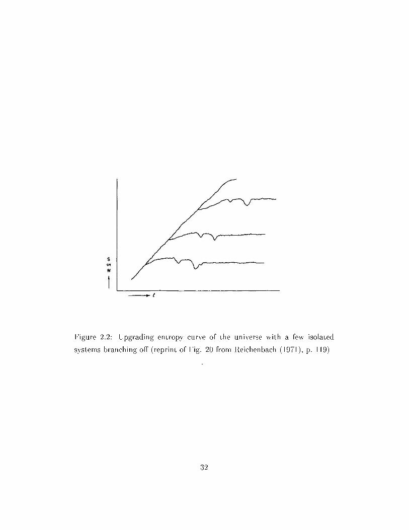
Figure 2.2: Upgrading entropy curve of the universe with a few isolated
systems branching o (reprint of Fig. 20 from Reichenbach (1971), p. 119)
.
32
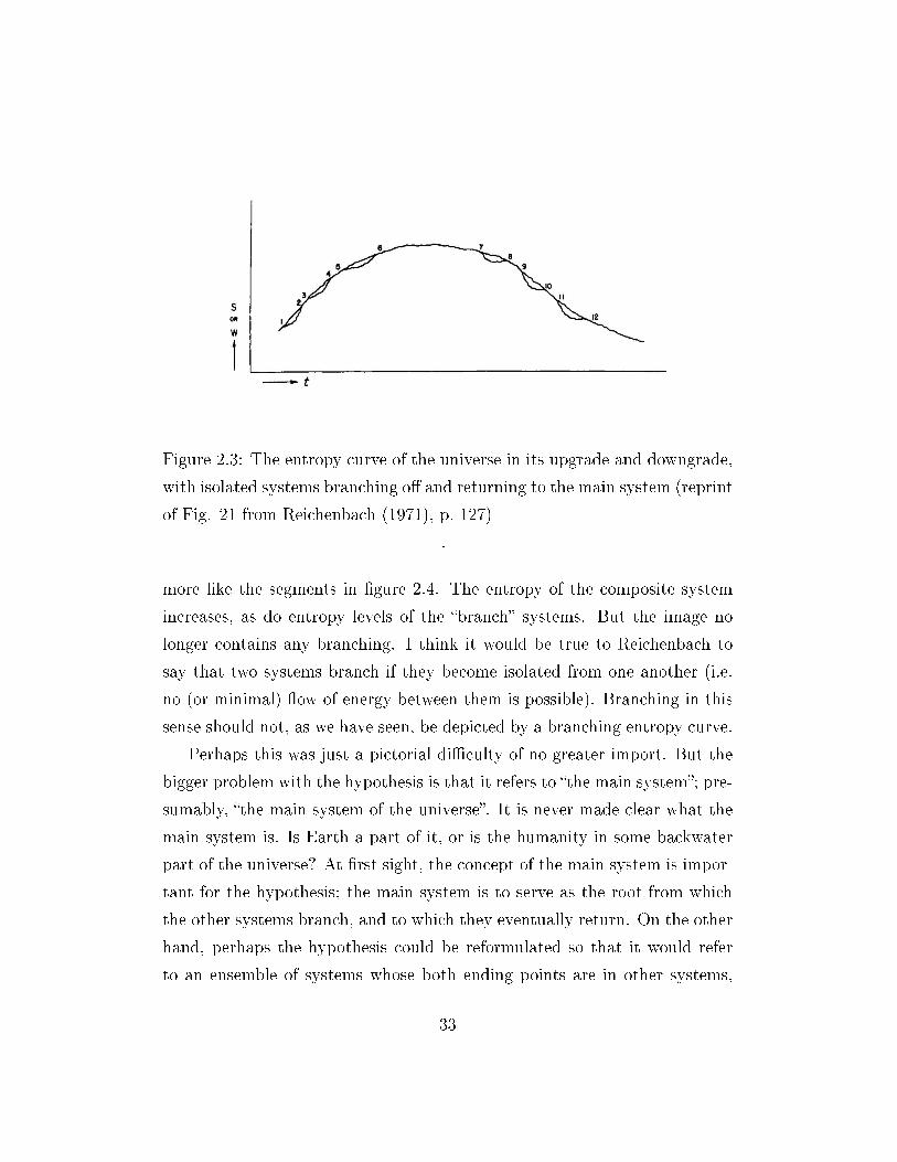
Figure 2.3: The entropy curve of the universe in its upgrade and downgrade,
with isolated systems branching o and returning to the main system (reprint
of Fig. 21 from Reichenbach (1971), p. 127)
.
more like the segments in gure 2.4. The entropy of the composite system
increases, as do entropy levels of the branch systems. But the image no
longer contains any branching. I think it would be true to Reichenbach to
say that two systems branch if they become isolated from one another (i.e.
no (or minimal) ow of energy between them is possible). Branching in this
sense should not, as we have seen, be depicted by a branching entropy curve.
Perhaps this was just a pictorial diculty of no greater import. But the
bigger problem with the hypothesis is that it refers to the main system; pre-
sumably, the main system of the universe. It is never made clear what the
main system is. Is Earth a part of it, or is the humanity in some backwater
part of the universe? At rst sight, the concept of the main system is impor-
tant for the hypothesis; the main system is to serve as the root from which
the other systems branch, and to which they eventually return. On the other
hand, perhaps the hypothesis could be reformulated so that it would refer
to an ensemble of systems whose both ending points are in other systems,
33

Figure 2.4: Entropy of a system which divides from time to time into two
systems for a certain period.
and which are isolated from all other systems apart from their endpoints.
In this case, there would be no distinguished root, or main, systemand
similarly, there would be no need to use the name branch system instead of
simply saying system: all systems would have equal rights, so to speak. One
would also have to take care when accommodating the old Assumption 4 (In
the vast majority of branch systems, one end is a low point, the other a high
point) to the new hypothesis; what if a system K branches o a system L
at a point of L's high entropy, but, after a period of isolation, connects with
a system M at a point of M 's low entropy? I do not think these diculties
are insurmountable. It is feasible that one could reformulate Reichenbach's
hypothesis of the branch structure so that it would not refer to any main
system, while still capturing as much of the intentions of the original author
as possible. Then the task of deriving the PCC could be approached again.
A problem with this is that one would still be trapped with Reichenbach's
34

probability lattice approach and his notation. We prefer to pursue another
option and consider the chances of proving theorems related to the PCC us-
ing the machinery of modern probability theory. This endeavour is taken
up in chapter 6.
What do the initial examples illustrate?
As we said earlier on, Reichenbach himself claims that in his book probabil-
ity is always to be understood as a limit of a relative frequency. This would
seem to preclude ascribing probability to token, unrepeatable events; in
other words, there should be no single-case probabilities. However, we al-
ready quoted passages from Reichenbach (1949) indicating that there is an,
albeit elliptic, way of speaking about constructs which are to serve as a sub-
stitute for them in Reichenbach's theory. How should we, then, understand
the initial examples of common-causal reasoning oered by the author (and
quoted here on p. 22), the re and the wind, the burned-out bulbs, and the ill
actors? The common cause is invoked after the occurrence of a single event
is observed. At the end of section 2.1.2 we claimed that no beliefs about
the probability of such an event should be formed just because of a single
occurrence. Reichenbach seems to agree, writing on p. 158, not long after
the examples have been presented, (...) we assume that A and B have been
observed frequently; thus it is possible to speak about probabilities P (A),
P (B) and P (B | A) (...). So, in the initial examples we are not supposed to
think of probabilities, let alone correlations. Therefore they cannot be of any
support for the principle in its correlation formulation; they only illustrate
the coincidence formulation in action.
Remember, though, that the two features Reichenbach advertised as due
to which a common cause has explanatory value stem from the common cause
being a middle link in a conjunctive fork. Since the denition of the fork is
probabilistic, if we know nothing about the probability of the given common
35

cause C, we cannot judge whether it is the middle link in a conjunctive fork
ACB, and so cannot benet from the above-mentioned features: (1) that the
correlation disappears when the events A and B are considered conditional
on C, and (2) that the correlation is derivable from the conjunctive fork
condition. These two features show us why the PCC may be promoted as
one of the principles guiding the human search for explanation, but only in
its formulation referring to a correlation (p. 25), not in the one bringing up
an improbable coincidence (p. 22).
In conclusion, Reichenbach's initial examples illustrate only the coinci-
dence formulation of the principle, which lacks the important explanatory
features of the correlation formulation.
On forks open to the past
First let us ask about sucient conditions for a triple of events ACB to con-
stitute a conjunctive fork. Are the statistical requirements 2.3-2.6 enough?
Consider some events A, B and their common cause C, which operates in a
deterministic way: P (A | C) = P (B | C) = 1, P (A | C⊥) = P (B | C⊥) = 0.
Notice that
P (AC | B) = 1 = P (A | B)P (C | B);
P (AC | B⊥) = 0 = P (A | B⊥)P (C | B⊥);
P (A | B) = 1 > 0 = P (A | B⊥);
P (C | B) = 1 > 0 = P (C | B⊥),
so the triple ABC satises the statistical requirements for being a conjunctive
fork, with B being the middle link. But, if forks are to represent causal
relations, then ABC cannot be a conjunctive fork, because it is not a fork
in the rst place. The moral is this: prior causal knowledge is needed to
36

determine whether the fact that a triple of events satises conditions 2.3-2.6
means that the triple constitutes a conjunctive fork. We dier in this opinion
from e.g. Salmon, who considers the statistical conditions as denitional12
for the notion of the conjunctive fork, but (for unrelated reasons) assuming
additionally that none of the probabilities occurring in the requirements may
be equal to 0 or 1, and who would thus be unaected by my counterexample.
Conjunctive forks open to the past would of course (just as any exam-
ples of two correlated any events with neither a common eect nor a com-
mon cause) constitute counterexamples to the PCC. Reichenbach claims that
whenever a conjunctive fork AEB is found such that E is a common eect of
A and B, there exists an event D, which is a common cause of A and B, and
is the middle link of a conjunctive fork ADB. There exist no conjunctive
forks open to the past.
Reichenbach oers both a general argument and some specic examples.
The argument is of a teleological nature and refers to the fact that we do not
accept nal causes as explanations. Final causes are deemed incompatible
with the second law of thermodynamics in the preceding chapter (§18 of
Reichenbach (1971)); a general question is asked: how are we to explain the
presence of a highly ordered (and so, very improbable) state of a system
(such as a trace of footprints in the sand)? Reichenbach's answer is that
we are supposed to look for an interaction at the lower end of the branch
run through by an isolated system which displays order, which will be the
cause; the state of order is the eect (p. 151). The ordered state is, then,
to be understood as a post-interactive state. Since the overarching goal is
to provide a denition of time direction (as we have seen Reichenbach doing
in the following chapter§19 of Reichenbach (1971)by dening what is to
be meant by past), the author proposes to consider the system containing
the beach with the footprints in reverse time (p. 153). We would have to
12 See Salmon (1984), p. 159-160.
37

think of the ordered state as a pre-interactive state, and so, in our search
for its explanation would end up with a nal cause (The wind transforms
the molds in the sand into the shapes of human feet in order that they will
t the man's feet when he comes, ibid.); in general, we would explain the
improbable coincidences by their purpose rather than by their cause (ibid.).
Since this is implausible, the conclusion is that the direction of time should be
dened, generally speaking, from interaction to order, rather than the other
way round. And so, if we dene the direction of time in the usual sense,
there is no nality, and only causality is accepted as constituting explanation
(p. 154).
Unfortunately, the nonexistence of conjunctive forks open to the past
would follow from the above only had it been established that such a con-
junctive fork would necessitate the usage of nal causes. This would only
be the case if (1) every correlation between events having a common eect
but no common cause (i.e. events being the extreme elements of a causal
fork open to the past) had an explanation; (2) the only accepted way of
explaining such a correlation would be to refer to an event in their causal
future. But Reichenbach does not give arguments for any statements similar
to the two above; in fact, he seems to rely on an (unsupported) fundamental
principle that every correlation whatsoever has an explanation. Notice also
the curious jump from the epistemic to ontological perspective on p. 163: A
common eect cannot be regarded as an explanation and thus need not ex-
ist. In general, it does not seem that Reichenbach's general argument for the
nonexistence of open conjunctive forks with a common eect as the middle
element holds up under scrutiny, mainly due to the trick of deriving the on-
tological conclusion from epistemic premises (like the universal requirement
for explanation for correlations).
Coming now to the specic examples, the author gives an instance of a
fork open to the past on p. 163, aiming to convince the reader that the fork
38
cannot be conjunctive. Let us quote a part of the example:
For instance, when two trucks going in opposite directions along
the highway approach each other, their drivers usually exchange
greetings, sometimes by turning their headlights on and o. We
have here a fork AEB, where E is the exchange of greetings,
which is a common eect of the coincidence of the trucks, that
is, of the events A and B (Reichenbach (1971), p. 163).
It is not evident how we should think about probabilities in this case, but
one way would be to hold xed a fragment X of some highway, and let A be
the event there is a truck going in the eastern direction in the fragment X,
B be the event there is a truck going in the western direction in the fragment
X, and E two trucks going in the opposite directions in the fragment X are
ashing their headlights. We can check whether the events occur e.g. every
second. Then it is very likely that E⊥ does not screen o A from B, so the
three events indeed do not form a conjunctive fork. Still, a general argument
against the mere possibility of such a fork open to the past is needed.
A related problem appears in Salmon (1984), where on p. 164-165 an
example oered by Frank Jackson of a conjunctive fork open to the past is
discussed.
[C]onsider a case that involves Hansen's disease (leprosy). One
of the traditional ways of dealing with this illness was by segre-
gating its victims in colonies. Suppose that Adams has Hansen's
disease (A) and Baker also has it (B). Previous to contracting
the disease, Adams and Baker had never lived in proximity to
one another, and there is no victim of the disease with whom
both had been in contact. We may therefore assume that there is
no common cause. Subsequently, however, Adams and Baker are
39

transported to a colony, where both are treated with chaulmoogra
oil (the traditional treatment). The fact that both Adams and
Baker are in the colony and exposed to chaulmoogra oil is a com-
mon eect of the fact that each of them has Hansen's disease.
This situation, according to Jackson, constitutes a conjunctive
fork A,E,B, where we have a common eect E, but no common
cause (Salmon (1984), p. 164)
To check whether the statistical conditions are satised, one has of course
to check e.g. probabilities P (A | E⊥) and P (A⊥ | E⊥). But how should we
do this? We had already assumed that Adams has Hansen's disease and that
he is in the colony. How can we ask about the probability that he is not ill
or that he is not in the colony? Certainly we are not evaluating a probability
of a counterfactual statement13. Instead, it is evident from p. 165 of Salmon
(1984) that the author calculates the probability P (B⊥ | E) simply by taking
the proportion of people in the colony who are not ill (the medical personnel)
to all members of the colony. But in this way he transforms a constant into a
variable and it is no longer possible to dierentiate between events A and B,
since both of them are a randomly chosen man from the colony has Hansen's
disease.
It would seem, then, that Reichenbach's account lacks a general argument
for his point, and Salmon's considerations on the subject are defective. On
the other hand, we have to admit we have been unable to nd a real-world
example of a conjunctive fork open to the (causal) past. Still, consider the
following hypothetical situation: a group of 10000 men (labeled, for our con-
venience, from ”1” to ”10000”) considered as representative for the region is
tested for hypocalcemia (E), lactose intolerance (A) and hypoparathyroidism
(B). Lactose intolerance and hypoparathyroidism have no known common
13 Which is a task attempted later on e.g. in chapter 7 of Pearl (2000).
40

cause, while it is known that each may lead to hypocalcemia. If:
• men labeled from 1 to 1000 (and only them) have hypocalcemia;
• men labeled from 1 to 500 and from 1001 to 4000 (and only them) have
lactose intolerance;
• men labeled from 251 to 750 and from 3001 to 6000 (and only them)
have hypoparathyroidism;
then it is straightforward to see (if we accept the move from relative fre-
quencies to probability: here, for the sake of the example, we can simply say
that the population from which the sample had been drawn is identical to
the sample) that the fork AEB satises the requirements from the denition
of a conjunctive fork (2.3-2.6). However, the middle element of the fork is
a common eect of the two other elements, which have no known common
cause. I do not see why such situations should be impossible; yet again, I
have been unable to nd a real example.14
(A dierent matter is whether a conjunctive fork open to the past and
a conjunctive fork AEB with the middle element E being a common eect
of A and B, such that there is no common cause C of the two events such
that the fork ACB is conjunctive are to be identied. They certainly are
on the assumption that past in the rst expression is to be understood as
causal past).
2.4 The PCC after Reichenbach
Reichenbach's principle was heavily promoted in the 70s and 80s by Wesley
Salmon (e.g. Salmon (1971)). More recently, it has been an inspiration for a
14 Another hypothetical example of a conjunctive fork not pointing to a common cause
was also presented in Torretti (1987).
41
fundamental condition in the eld of representing causal relations by means
of directed acyclic graphs (see chapter 5). However, a plethora of counter-
arguments appeared; most are gathered and discussed in Arntzenius (1992).
Some, e.g. Sober's (1988) sea levels vs. bread prices argument, were directed
against any sort of general requirement of common causal explanation. Oth-
ers lead a few philosophers (e.g. Salmon (1998b)15 and Cartwright (1988))
to transform Reichenbach's idea, preserving the principle's requirement of
common causes for correlations, but changing the screening o condition,
or supplementing it with other conditions. It would be of no use for the
current essay to discuss all these ideas in detail: our focus is on the notions
of common cause revolving around the original idea of screening o. We
will however describe the three arguments we would rate as most important.
These are:
• the argument from Bell inequalities, to which we will devote the whole
chapter 5;
• the argument from conservation principles, described in section 2.4.1;
• and the sea levels / bread prices argument, described in section 2.4.2.
Later, in the 90s, Reichenbach's idea in the form of PCC 4 was defended
in papers by M. Rédei, G. Hofer-Szabó and L. Szabó (e.g. Hofer-Szabó et al.
(2000)): rather then confronting the earlier counterarguments to Reichen-
bach's idea directly, the authors proposed mathematical arguments in favour
of PCC 4. It is to this area of research that the current study aims to con-
tribute in chapters 6 and 7. Let us rst describe the two arguments against
Reichenbach's principle we just mentioned above.
15 Originally published in 1978.
42
2.4.1 The argument from conservation principles
We will cite the formulation of this argument given in Arntzenius (1992),
since it seems to be the most concise:16
Suppose that a particle decays into 2 parts, that conservation
of total momentum obtains, and that it is not determined by
the prior state of the particle what the momentum of each part
will be after the decay. By conservation, the momentum of one
part will be determined by the momentum of the other part. By
indeterminism, the prior state of the particle will not determine
what the momenta of each part will be after the decay. Thus
there is no prior screener o. (Arntzenius (1992), p. 227-8.)
There are numerous variants of this argument in the literature; the ver-
sion from Salmon (1998b) refers to Compton scattering. In the same paper
Salmon, as an answer to the problem, proposes the introduction of another
kind of fork (apart from the conjunctive variety), the so called interactive
fork. Probabilistically, an interactive fork with the middle element C and
two extreme elements A and B diers from a corresponding conjunctive fork
in that instead of the two screening o requirements a single condition is
introduced: namely, P (AB|C) > P (A|C)P (B|C). That it is met by the
examples built around some conservation principle becomes evident when we
notice that in such examples (if C is the state of the compound before the
splitting) 1 = P (A|B ∧ C) > P (A|C) .
Notice that the argument only implicitly refers to probability, via the
notion of screener o. No probability spaces are dened. Therefore it is an
argument against PCC 2. It is not clear what force it would have against
PCC 4, whichas mentioned abovehas been mathematically proven to
16 It is labeled Indeterministic Decay with Conservation of Momentum and attributed
to van Fraassen (1980).
43
be true. One would have to consider all probability spaces which could be
used to describe the decay event and its consequences; then the extensions
of those spaces which contain common causes in the sense of PCC 3; and
nally ponder the question whether such events could have anything to do
with what we would naturally accept as a common cause of the properties
of the two particles.
An ad hoc solutionbut not without intuitive meriton part of a pro-
ponent of PCC 2 could be that correlations which arise due to conservation
principles do not demand (additional) explanation: if we know the princi-
ple at work, we do not require anything more to explain the correlation.
Salmon's way out (philosophically rooted in the distinction between causal
processes and interactions) was simply to incorporate interactive forks into
the picture and to say that some correlations are explained by events which
together with the correlated events form a conjunctive fork, but some others
demand as their explanantes the middle elements of interactive forks.17
2.4.2 The sea levels vs. bread prices argument
This argument rst appeared in Sober (1988) and was elaborated in Sober
(2001). The most important thing is that, in the parlance of the current
essay, it is an argument for abandoning PCC 1 for PCC 2: not all correlations
demand a common causal explanation.18 By reductio: otherwise a correlation
between Venetian sea levels and British bread prices would demand such an
explanation, while it surely does not. More extensively:
Consider the fact that the sea level in Venice and the cost of bread
in Britain have both been on the rise in the past two centuries.
17 In fact, Salmon himself eventually espoused a variant of the conserved quantity
theory, see Salmon (1998a).18 Which demand and which do not is in Sober's account decided by our background
theory.
44

Both, let us suppose, have monotonically increased. Imagine that
we put this data in the form of a chronological list; for each date,
we list the Venetian sea level and the going price of British bread.
Because both quantities have increased steadily with time, it is
true that higher than average sea levels tend to be associated
with higher than average bread prices. The two quantities are
very strongly positively correlated.
I take it that we do not feel driven to explain this correlation
by postulating a common cause. Rather, we regard Venetian sea
levels and British bread prices as both increasing for somewhat
isolated endogenous reasons. (Sober (1988), p. 215.)
There are several strands of thought in the literature on the argument.
We will try to label and shortly discuss them.
1. No correlation at the level of changes. Forster (1988) was the
rst to notice that, while the sea levels and bread prices are correlated,
their respective changes are not: year by year, both the former and the
latter increases. It is hard to estimate the import of this observation:
in fact, the lack of correlation on the level of changes would perhaps
intuitively indicate lack of causal connection, which would strengthen
Sober's point. In any case, Sober (2001) presented an example stem-
ming from evolutionary biology in which the correlation persists on the
level of changes of the values of two attributes, and in which also no
common causal explanation is expected.
2. Mixing. Some authors (e.g. Spirtes, Glymour & Scheines (2000), p. 33-
37) point outgoing back to the work of G. Udny Yule in the begin-
ning of the XXth centurythat a correlation between attributes in a
population may be the result of mixing two populations in which the
45

attributes are not correlated. The solution of Spirtes, Glymour and
Scheines, working in the formalism of directed acyclic causal graphs
(more on that in chapter 4), is to treat belonging to one of the given
subpopulations as an attribute in the big population, which enables
them to recover the proper conditional independencies. This amounts
to saying that whenever such a mixing occurs, the correlation is ex-
plained by the mixing itself. The authors treat (p. 37) Sober's example
as a case of mixing (in fact, they claim that his point was similar to
Yuly's) and consider the case closed. This is consistent with PCC 2: if
we know that such a mixing occurred, then we either do not think of
the correlation as demanding an explanation at all, or we consider it
explained by the mixing itself. However, the particular example of sea
levels and bread prices does not lend itself easily to the mixing inter-
pretation. What are the two populations to be mixed? They cannot
be the 200 years, since there is only one set of years to be considered.
Thinking of Sober's example as a case of mixing seems to require some
serious mind-twisting. It might be better to look at it as consisting of
two monotonically increasing time series.
3. Time series. Hoover (2003) observes that the data given by Sober
allow us to infer that there is a correlation on the level of frequencies,
but it does not necessarily follow from that that there is a correlation
on the level of probabilities. (...) most statistical inference and most
of our own probabilistic intuitions are based on stationary probability
distributions (p. 532).
A rigorous discussion of this point would require numerous denitions,
so let us settle for a more informal account. A necessary condition for a
time series to be stationary is that the covariance between the values
of the series at dierent times depends only on the temporal distance
46

between them (p. 532). Of course, a monotonically increasing time
series is not stationary. However, for any time series we can consider
a series of dierences between the consecutive values of the series. It
may very well happen that the series is stationary (consider e.g. the
case of the series of consecutive natural numbers from 1 to 200); in
that case the original series is said to be integrated of order 1, or I(1).
As Hoover points out (p. 545-546), a linear combination of two I(1)
time series is in general also I(1), but it may happen that there exists a
linear combination which is stationary: only in this case (in which we
say the time series are cointegrated) the data constitute evidence for
probabilistic dependence. As Reiss (2007) puts it (p. 184), inferring
from a sample correlation to a probabilistic dependence means that
one takes the most likely data-generating process to be stationary. In
Sober's case we are likely to assume otherwise. Hoover proposes to
let PCC apply to cases in which the correlated series are either (1)
both stationary or (2) both I(1), but cointegrated. Since Sober's time
series are not cointegrated, they do not constitute a counterexample to
Hoover's version of the principle.
We would like to divert attention to a dierent issue. Why do we think
the correlation between Venetian sea levels and British bread prices does not
demand explanation? Is there more to say on the topic than Hoover's idea
of referring to the two time series being nonstationary but not cointegrated?
2.4.3 Which correlations demand explanation?
Various authors have eshed out the beginning part of PCC 2 dierently.
Some say that only improbable correlations demand explanation. This can
mean simply statistically signicant (Forster (1988), p. 539), unexpected
or surprising (Unk (1999)), or e.g. such that the assumption that it arises
47
from causally unrelated processes will render it unexpected, with a formally
dened notion of unexpected (Berkovitz (2000), p. 65).
There is a sense, meta-probabilistic in a way, in which a correlation can
be rigorously thought of as improbable. Consider a nite probability space
〈Ω,F , P 〉, in which Ω has n elements, F is the set of all subsets of Ω, and for
any A ∈ F , P (A) = card(A)n
. Suppose two subsets A and B of Ω are chosen at
random in the sense that every member of Ω has a chance of 12of belonging to
A and the same chance of belonging to B. It can be checked using a moderate
dose of combinatorics and Stirling's approximation that with n approaching
innity, the chance of arriving at a probabilistically independent pair by the
process just outlined approaches 0. Informally, we would say that in a big
enough population, (almost) everything is correlated with (almost) every-
thing. But the proportion of pairs such that∣∣P (AB) − P (A)P (B)
∣∣ < 0.05
(which is one, quite arbitrary, way of saying weakly correlated pairs) to all
pairs increases with n, toostrongly correlated pairs are infrequent in this
sense (i.e., it is hard to come upon them by pure chance). We have to confess
that for this statement we only have an argument of consulting statistical
softwarewe used the R software to track the proportions of weakly and
strongly correlated pairs in populations of increasing sizes. So, if we do not
possess any knowledge about the genesis of some two events, it should be
natural to expect them to be correlated, but only weakly. The subjective de-
gree of this expectation should vary with the size of the population involved.
However, this approach is too abstract to properly illustrate our beliefs re-
garding the probabilistic nature of phenomena we observe in the world: we
in general do not start with a clean slate, but possess some background
knowledge which inuence our beliefs regarding such issues.
In his account19, to the condition of improbability Berkovitz also adds,
without further commentary, that the correlation should be non-accidental
19 Berkovitz (2000).
48

(p. 56). What does it mean for a correlation to be accidental? Perhaps it
will be illuminating to consult a clarication of types of correlation from Haig
(2003), where a reinterpretation of the notion of spuriousness is argued for.
A traditional (see e.g. Hitchcock (2010)) example of a spurious correlation
is that of a barometer and a storm. Shortly speaking, a spurious correlation
arises between events which are not directly causally connected, but have a
common cause. Haig notices that the word spurious might be misleading
in this case, since the correlation is due to a genuine causal connectionin
contrast with the correlations which arise e.g. from a sampling bias. Haig's
classication is presented in gure 2.5.
correlation
HHHHHH
accidental
genuine
PPPPPP
nonsense
spurious
XXXXXXXX
direct
indirect(spurious)
Figure 2.5: A classication of correlations from Haig (2003).
A nonsense correlation is that for which no sensible, natural causal
interpretation can be provided (Haig (2003), p. 127). Haig's examples are
the high positive correlation between birth rate and number of storks for
a period in Britain and the negative correlation between birth rate and
road fatalities in Europe over a number of years. It is clear, I think, that
Haig would interpret Sober's examples as falling into this category. Spurious
correlation are these which are not brought about by their claimed natural
causes, but by accident, for example due to sample selection bias, use
of an inappropriate correlation coecient, large sample size, or errors of
49

sampling, measurement, and computation (Haig (2003), p. 128). Of the
genuine correlations, the indirect are due to either common or intervening
causes (p. 129)20. Notice that if we formulate our principle as any non-
accidental correlation between events which are not directly causally related
or logically dependent is due to a common cause, it is clearly true under
Haig's account. Whether the common cause in question should screen o
the correlated events is a dierent matter.
On the other hand, Sober would most likely say thatin the cases like the
sea levels vs. bread pricesthere is a perfectly natural causal interpretation
which consists of two separate causal explanations of the two phenomena,
and thus such correlations should not be counted as nonsense. But let us
examine this line of reasoning. Suppose that there is an explanation E for
the ongoing rise of sea levels; perhaps the melting of sub-polar glaciers. E
explains why the data for sea levels in Venice form a monotonic time series.
Likewise, suppose there is some explanation F for the ongoing rise of bread
prices; perhaps a combination of high taxes and deteriorating crop levels.
F explains why the data for bread prices in Britain form a monotonic time
series. But this does not yet explain the correlation in question. But why
is A higher than average in the given time period precisely whenever B is?
The only reason we can nd is that the processes E and F are active in the
same time period. If this is accidental, then the correlation between A and
B should be deemed as accidental, too. Van Fraassen (1991, p. 350) uses the
word coincidence in this context.
20 A correlation between X and Y can arise partially due to an intervening cause if
there is a cause Z which with X jointly produces Y .
50

2.5 An epistemic position
It is interesting that in recent years two diametrically opposed approaches
to PCC have emerged: one (by Rédei, Hofer-Szabó and Szabó, discussed in
chapter 7) we could label as maximalist, which aims to prove that any cor-
relation has an explanation by means of a common cause if the probability
space is suitably chosen, and one perhaps aptly labeled as minimalist, due
to Reiss (2007). The latter renders the PCC as an intrinsically epistemic
principle. Since it seems to have an illustrative purpose and amounts to say-
ing if there is no conicting knowledge, correlation is evidence for causation,
we will only give the formulation here without extensive discussion:
PCC(Reiss). The proposition e = Random variables X and Y are
(sample or empirically) correlated is prima facie evidence for the hypothesis
h = X and Y are causally connected. If all alternative hypotheses hai
(e.g. the correlation is due to sampling error, the correlation is due to the
data-generating processes for X and Y being non-stationary, X and Y are
logically, conceptually or mathematically related) can be ruled out, then e
is genuine evidence for h (Reiss (2007), p. 193).
The epistemic nature of the principle is evident from its use of the notion
of evidenceno existential statements about the world are to be inferred
from other statements of a similar nature; the principle concerns the shaping
of our conception of the causal structure of the world. The principle is
eminently fallible because we may simply have wrong evidence against the
hypotheses alternative to the one of the existence of a common cause.
Before we tackle the issue of Bell inequalities, it is tting to devote a
chapter to the formal features of various notions related to screening o.
51
Chapter 3
Screening o and explanation:
formal properties
Arguably, the most important feature of Reichenbach-style common causes
is that they screen o their eects. In this chapter we will consider a few
constructions based on this idea which extend, or transform, Reichenbach's
original notion.
A part of literature refers to events dened as meeting Reichenbach's
conjunctive fork conditions as (Reichenbachian) common causes; see e.g.
Hofer-Szabó & Rédei (2004). Hofer-Szabó, Rédei & Szabó (2000) and Hofer-
Szabó & Rédei (2006) even go so far as to state that Reichenbach himself
dened common causes as the middle elements of conjunctive forks with
correlated extreme elements; in other words, that fullling the statistical re-
quirements for being the middle element of a conjunctive fork is sucient
to be a common cause for the correlated events. Due to the reasons already
presented in section 2.3 we are reluctant to adhere to this tradition. Nev-
ertheless, the main results of this work (see chapter 6) pertain to problems
posed in various papers by the above-cited authors. Therefore, some slight
terminological changes are in order.
52

Denition 9 [Statistical Common Cause] Let 〈Ω,F , P 〉 be a probabilityspace. Let A,B ∈ F . If there exists C ∈ F dierent from both A and B
such that
P (AB | C) = P (A | C)P (B | C);
P (AB | C⊥) = P (A | C⊥)P (B | C⊥);
P (A | C) > P (A | C⊥);
P (B | C) > P (B | C⊥),
then C is called a statistical common cause of A and B.
It is intuitive that a similar notion could be considered, with the dier-
ence that it would permit the cause to be more complicated than a simple
yes / no event. This is indeed the path taken without further comment
by van Fraassen (1982), but only the screening o requirement is retained.
A generalization which takes into account also the conditions of statistical
relevance was developed by Hofer-Szabó & Rédei (2004); the resulting con-
structs were called Reichenbachian common cause systems, but, for reasons
given above, we will abstain from the adjective Reichenbachian.
In view of the denition of statistical relevance (denition 7, p. 12) we can
say that a statistical common cause C is positively statistically relevant for
both its eects, or that in such a case the pair C,C⊥ is statistically relevantfor the same events; it would be wrong to say that C,C⊥ is positively
relevant, since one of its elements lowers the probability of the eects.
Denition 10 [Statistical Common Cause System] Let 〈Ω,F , P 〉 be aprobability space. A partition of unity of F is said to be a statistical common
cause system (SCCS) for A and B if it satises the statistical relevance
condition w.r.t. A and B, all its members are dierent from both A and B,
and all its members are screener-os for the pair.
53

The cardinality of the partition is called the size of the statistical common
cause system.
Statistical common cause systems come in dierent cardinalities; it was
proven in Hofer-Szabó & Rédei (2006) that SCCSs of arbitrary nite size
exist. However, for some time it has not been clear which range of cardi-
nalities is admissible. The problem whether innite SCCSs exist is posed in
Hofer-Szabó & Rédei (2004). We will now show that
Theorem 1 (Wro«ski & Marczyk (2010)) The greatest possible cardi-
nality of an SCCS is ℵ0.
Proof:
1. No uncountable SCCSs exist. To see this, suppose that in some
probability space 〈Ω,F , P 〉 an SCCS Cii∈I of size greater than ℵ0 ex-
ists. Since all elements of the SCCS are screener-os, they have to have
positive probabilityotherwise the required conditional probabilities are not
dened. But we know from measure theory (see e.g. Theorem 10.2 in Billings-
ley (1995), p. 162) that this is impossible, since the SCCS is a partition of
unity of F and so the set of its non-zero probability members can only be
countable.1
2. We will now construct an example of a countably innite SCCS.
1The reader may prefer conditional probabilities given probability zero events to be
always equal to 0, or 1 (see e.g. Adams (1998), p. 57). In these cases we note that for some
distinct k, l ∈ I, P (A | Ck) = P (A | Cl), which violates the statistical relevance condition.
54

Let 〈[0, 1),W, λ〉 be a classical probability space with W being the set of
all Lebesgue-measurable subsets of the real interval [0, 1) and λ being the
Lebesgue measure. Put
Cn :=
[2n − 1
2n,2n+1 − 1
2n+1
);
C := Cnn∈N
It is evident that if n 6= m (n,m ∈ N), Cn∩Cm = ∅ and that⋃C = [0, 1),
so C is a countably innite partition of [0, 1). Notice that for any natural n,
λ(Cn) = 12n+1 .
For any n ∈ N, we want both λ(A ∩ Cn) and λ(B ∩ Cn) to be equal to1
(n+2)·2n+1 . To improve the clarity of the notation below, put ln = 1(n+2)·2n+1 .
Dene
A :=∞⋃n=0
[2n − 1
2n,2n − 1
2n+ ln
);
B :=∞⋃n=0
[2n − 1
2n+n+ 1
n+ 2· ln,
2n − 1
2n+n+ 1
n+ 2· ln + ln
)
55

From the above denitions it follows that
λ(B | Cn) = λ(A | Cn) =λ(A ∩ Cn)
λ(Cn)=
1(n+2)·2n+1
12n+1
=1
n+ 2;
whereas
λ(A ∩B | Cn) =λ(A ∩B ∩ Cn)
λ(Cn)=
(1− n+1n+2
) · 1(n+2)·2n+1
12n+1
=
=
1(n+2)2·2n+1
12n+1
=1
(n+ 2)2
and so
λ(A ∩B | Cn) = λ(A | Cn)λ(B | Cn),
which means that C satises the screening-o condition.
Now, let m,n ∈ N,m 6= n. Without loss of generality assume m > n. It
follows that
λ(A | Cn) =1
n+ 2>
1
m+ 2= λ(A | Cm)
and
λ(B | Cn) =1
n+ 2>
1
m+ 2= λ(B | Cm).
Therefore the dierences λ(A | Cm)− λ(A | Cn) and λ(B | Cm)− λ(B | Cn)
have the same sign and are nonzero, so(λ(A | Cm)− λ(A | Cn)
)(λ(B | Cm)− λ(B | Cn)
)> 0 (m 6= n)
which means that C satises the statistical relevance condition.
We have shown that in the space 〈[0, 1),W, λ〉 the countably innite set
C is an SCCS for 〈A,B〉.
56

3.1 The deductive explanatory feature
We have already said that one of the two explanatory features of statistical
common causes considered by Reichenbach was the deductive one; namely,
from the fact that the conjunctive fork conditions are satised for A, C and
B one can deduce the correlation between A and B. We have to justify
not reproducing here the original proof by Reichenbach, which was simple
and to the point, and using a bit more complicated argument instead. The
reason is that we want to use the following fact, which is a characterization of
correlation between two events in terms of their relations to a third event; the
relations being how close the event is to being a screener-o for the pair and
how statistically relevant it is for both events. The fact makes the deductive
feature of SCCs evident and will also be useful in various endeavours below.
Fact 1 If events A and B are correlated, that is,
P (AB) > P (A)P (B),
then for all events C such that 0 < P (C) < 1
P (AB|C)− P (A|C)P (B|C)
P (¬C)+P (AB|¬C)− P (A|¬C)P (B|¬C)
P (C)>
− [P (A|C)− P (A|¬C)][P (B|C)− P (B|¬C)]. (3.1)
Conversely, if there exists an event C such that 3.1 is satised, then events
A and B are correlated.
Proof: Assume that C is such that 0 < P (C) < 1. Write P (AB) as
P (AB|C)P (C)+P (AB|C⊥)P (C⊥), P (A) as P (A|C)P (C)+P (A|C⊥)P (C⊥)
57

and P (B) as P (B|C)P (C) + P (B|C⊥)P (C⊥). After straightforward calcu-
lations we see that
P (AB)− P (A)P (B) =
P (C)P (C⊥)[− P (A|C)P (B|C⊥)− P (A|C⊥)P (B|C)
]+
+ P (AB|C)P (C)− P (A|C)P (B|C)[P (C)
]2+
+ P (AB|C⊥)P (C⊥)− P (A|C⊥)P (B|C⊥)[P (C⊥)
]2. (3.2)
Considering the last two lines of the above equation, observe that
P (AB|C)P (C)− P (A|C)P (B|C)[P (C)
]2=
P (C)P (C⊥)[P (AB|C)− P (A|C)P (B|C)
P (C⊥)+ P (A|C)P (B|C)
]and
P (AB|C⊥)P (C⊥)− P (A|C⊥)P (B|C⊥)[P (C⊥)
]2=
P (C)P (C⊥)[P (AB|C⊥)− P (A|C⊥)P (B|C⊥)
P (C)+ P (A|C⊥)P (B|C⊥)
].
After substituting the two above expressions in equation 3.2 we can infer
that
P (AB) > P (A)P (B) ≡(P (AB|C)− P (A|C)P (B|C)
P (¬C)+P (AB|¬C)− P (A|¬C)P (B|¬C)
P (C)>
− [P (A|C)− P (A|¬C)][P (B|C)− P (B|¬C)]).
Therefore, if A and B are correlated, 3.1 is valid for any C of non-zero and
non-one probability. In the other direction, if we nd some event C for which
3.1 is valid, due to the above equivalence we can deduce the correlation of A
and B.
58
It is immediate from the inspection of the form of 3.1 that if C is a
statistical common cause of A and B, then 3.1 holds. We can thus claim the
following (which was originally proven in Reichenbach (1971)):
Corollary 2 Let 〈Ω,F , P 〉 be a probability space. Let A,B ∈ F . If C ∈ Fis a statistical common cause of A and B, then A and B are correlated.
A similar result for statistical common cause systems is due to Hofer-
Szabó & Rédei (2004):
Fact 3 (Hofer-Szabó & Rédei (2004)) Let 〈Ω,F , P 〉 be a probability space.Let A,B ∈ F . If C ⊆ F is a statistical common cause system of A and B,
then A and B are correlated.
3.2 In search for common causes, screening o
is enough
Let us now change the perspective. Suppose we know that some events A and
B are correlated and we are looking for a statistical common cause. It turns
out that it is enough to nd an event C such that both it and its complement
screen o A and B; it is then guaranteed that either C or C⊥ will be an SCC
for the correlated events. This is because in such a situation the left-hand side
of inequality 3.1 will be 0, therefore [P (A|C)−P (A|¬C)][P (B|C)−P (B|¬C)]
will be positive, which means that both dierences have the same signso
either C or C⊥ will meet the conditions for being a statistical common cause
for A and B. Let us summarize this in a corollary, for future reference in
chapter 6:
Corollary 4 Let 〈Ω,F , P 〉 be a probability space. Let A,B,C ∈ F . SupposeA and B are correlated. If both C and C⊥ screen o A from B, then either
C or C⊥ is a statistical common cause of A and B.
59
In other words, ifgiven two correlated eventswe nd a two-element
partition of the unity of the space such that both its elements screen o the
correlation, we are guaranteed that (1) one of the elements is a statistical
common cause and (2) one of the elements is positively statistically relevant
for both correlated events, which is a somewhat intuitive feature of probabilis-
tic causes (this being one of the biggest foundational issues of probabilistic
causality). We separate (1) from (2), because they can come apart when we
switch our attention to more than 2-element partitions of the unity of the
space which consist of screener-os only. The following examples will show
that, in general, if such a partition of unity (which we will call a screener
system, see the denition below) has more than 2 elements, we can neither
infer that we have found an SCCS, nor that at least one of its elements is
positively statistically relevent for both A and B.
Denition 11 [Screener System] Let 〈Ω,F , P 〉 be a probability space.
Let A, B ∈ F . If C is a partition of unity of F , then C is called a screener
system for A and B if all elements of C screen o A from B.
We already know that a two-element screener system for correlated A
and B has to contain a statistical common cause for the two events. Both
examples to follow will present, for given correlated events A and B, three-
element screener systems which will not be statistical common cause systems.
Example 1 Consider a probability space 〈Ω,F , P 〉, where Ω = 1, . . . , 100 ⊆N, F = Ω2, and P is the uniform measure on F (for any x ∈ Ω, P (x) =
1100
). Consider events A = 1, . . . , 30 and B = 11, . . . , 40 ∪ 51, . . . , 85.P (AB) = 2
10> 195
1000= P (A)P (B), so A and B are correlated. Dene
C := Cii∈0,1,2, where C0 := 11, . . . , 20, C1 := 1, . . . 10 ∪ 21, . . . , 50,
60

and C2 := 51, . . . , 100. Check that
P (AB|C0) = 1 = P (A|C0)P (B|C0);
P (AB|C1) = 14
= P (A|C1)P (B|C1);
P (AB|C2) = 0 = P (A|C2)P (B|C2),
therefore C is a screener system for A and B. However, P (A|C2) = 0 <
P (A|C1), but P (B|C2) = 710> 1
2= P (B|C1), which means that C does not
satisfy the statistical relevance conditions for A,B (see denition 7, p. 12),
and so is not a statistical common cause system for A and B.
In the above example both C0 and C1 were positively statistically relevant
for both A and B. We will now see that it may happen that no element of a
screener system is positively statistically relevant for any of the two correlated
events.
Example 2 Consider a probability space 〈Ω,F , P 〉, where Ω = 1, . . . , 6 ⊆N, F = Ω2, and P is the uniform measure on F (for any x ∈ Ω, P (x) =16). Consider events A = 1, 2, 3 and B = 2, 3, 4. P (AB) = 1
3> 1
4=
P (A)P (B), so A and B are correlated. Dene C := Cii∈0,1,2, whereC0 := 1, 2, C1 := 3, 4, and C2 := 5, 6. Check that
P (AB|C0) = 12
= P (A|C0)P (B|C0);
P (AB|C1) = 12
= P (A|C1)P (B|C1);
P (AB|C2) = 0 = P (A|C2)P (B|C2),
therefore C is a screener system forA andB. Notice, however, that P (B|C0) =12
= P (B|C⊥0 ), P (A|C1) = 12
= P (A|C⊥1 ), P (A|C2) < P (A|C⊥2 ) and P (B|C2) <
P (B|C⊥2 ). Therefore none of the elements of C is positively statistically rel-
evant for both A and Beven though C0 raises the probability of A and C1
raises the probability of B.
61
A part of the motivation for calling a statistical common cause a cause
in the rst place is that it raises the probability of both its eects. We now
see that, in general, in case of more than 2-element screener systems we do
not have the guarantee that one of its elements will do this job. On the other
hand, not all elements of a nite screener system for two correlated events A
and B may lower the probability of both A and B (we conjecture that the
fact holds also in the case of innite systems):
Fact 5 Let 〈Ω,F , P 〉 be a probability space. Let A, B be correlated events
in F . Suppose a nite C = Cii∈I is a screener system for A and B. Then,
for some i ∈ I, P (A|Ci) > P (A) or P (B|Ci) > P (B).
Proof: Suppose to the contrary, that for all i ∈ I, P (A|Ci) 6 P (A) and
P (B|Ci) 6 P (B). We know from our assumption that P (AB) > P (A)P (B).
But, since C is a partition of unity of F ,
P (AB) =∑i∈I
P (AB|Ci)P (Ci) =∑i∈I
P (A|Ci)P (B|Ci)P (Ci) 6
6 P (A)P (B)∑i∈I
P (Ci)︸ ︷︷ ︸1
= P (A)P (B),
therefore we arrive at a contradiction.
3.3 Common common constructs
It is one thing to look for a common cause of a single correlation; it is
another to ask whether two (or more) correlations can be explained by means
of the same common cause. These issues are important for the discussion
of the relationship between the PCC and Bell's inequalities, the topic of
chapter 4. In this section we will give formal denitions of common statistical
62
common causes and common screener systems, as well as notice a simple fact
regarding the existence of common screener systems for nite families of
correlations. For completeness we will also include the concept of common
statistical common cause systems, thoughto our knowledgeno results
concerning them have been published.
Denition 12 [Common SCC, Common Screener System, and Com-
mon SCCS] Let 〈Ω,F , P 〉 be a probability space. Let G ⊆ F2 be a family
of pairs of correlated events in F .
• An event C is called a common statistical common cause (CSCC)
for G (or for all pairs in G) if for every 〈A,B〉 ∈ G, C is a statistical
common cause for A and B.
• If C is a partition of unity of F , then C is called a common screener
system (CSS) for G if for every 〈A,B〉 ∈ G, C is a screener system for
A and B.
• If C is a partition of unity of F , then C is called a common statistical
common cause system (CSCCS) for G if for every 〈A,B〉 ∈ G, C is a
statistical common cause system for A and B.
Since it is nothing unusual for a correlated pair of events not to have a
statistical common cause in the given probability space (see chapter 6), it
is not surprising that not all pairs of correlated events have common SCCs.
Hofer-Szabó, Rédei & Szabó (2002) have established necessary conditions for
two correlated pairs of events having a common SCC. We will now show
that, in any space, a nite family of correlated pairs always has a common
screener system. Let us just note that in the case of a nite probability
space the problem is trivialit suces to construct a partition of the unity
63
of the event space from all singletons of the elements of the sample space2.
However, the screener system constructed this waywhile doing the job
can be huge. During the proof of fact 6 we will construct a more ecient
screener system.
Fact 6 Let 〈Ω,F , P 〉 be a probability space. Let G =Ai, Bi
i∈I ⊆ F
2 be
a nite family of pairs of correlated events in F . There exists a partition Cof the unity of F which is a common screener system for G.
Proof: Consider the set of atoms of the Boolean subalgebra of F gen-
erated by ∪G. Remove any empty atoms. Add any zero-measure atoms to
an arbitrary atom with non-zero measure. Notice that the resulting set C isa partition of unity of F . It is immediate that ∀i∈I∀C ∈ C either
P (AiBi|C) = 1 = P (Ai|C)P (Bi|C)
or
P (AiBi|C) = 0 = P (Ai|C)P (Bi|C)
(all probabilities are dened, because due to our precautions all elements of
C have positive measure). Therefore, every member of C screens o all the
correlations belonging to G. We conclude that C is a common screener system
for G.
Problem 1 Do innite families of correlations also always have common
screener systems?
2 If any of these singletons have zero probability, simply append them to arbitrary
singletons with non-zero probability.
64

3.4 Explanation via screenersthe general pic-
ture
In this section we will discuss constructs dierent from SCC(S)s, but which
nonetheless share the previously mentioned deductive explanatory feature.
Let us rst put some labels on the already introduced conditions, for future
reference:
P (AB|C) = P (A|C)P (B|C) (SCR(A,B,C))
P (A|C) > P (A|C⊥) (STAT(A,C))
P (AB) > P (A)P (B) (CORR(A,B))
The deductive explanatory feature of common causes postulated by Re-
ichenbach can be expressed as the fact that CORR(A,B) follows from
SCR(A,B,C), SCR(A,B,C⊥), STAT(A,C) and STAT(B,C). In general, let
us call a set of conditions deductively explanatory for CORR(A,B) if the
fact that all conditions from the set are satised entails positive correlation
between A and B. Of course, CORR(A,B) is trivially deductively ex-
planatory for CORR(A,B). Reichenbach's conjunctive fork criteria comprise
an example of non-trivial deductively explanatory set of conditions. We al-
ready said that screening-o alone has some explanatory value tied with the
vanishing of the correlation when conditional probability is considered. This
brings us to the following problem:
The screener-o classication problem. Apart from Reichenbach's
criteria for a conjunctive fork, are there any other interesting sets of condi-
tions which would contain SCR(A,B,C) and would be deductively explana-
tory for CORR(A,B)?
The word interesting is to mean non-trivial, to exclude explanations of
65

CORR(A,B) by CORR(A,B) or its equivalents which refer to A and B only.
Also, since the overarching goal is to nd an explanation for a correlation
between two events by means of a third event C, the explanatory condition
should refer to the third event in a non-trivial way.
From a bit dierent angle: an event C, which is a statistical common cause
for A and B, can be viewed as an explanation for the correlation between A
and B because its existence makes true a certain set of conditions which are
deductively explanatory for the correlation. We can ask a question: apart
from SCC (and the general concept of SCCS), are there dierent types of
screeners which could act as explanations for the same deductive reason?
3.4.1 Weakening the screening o condition
Before we provide a general classication of explanatory screeners, let us focus
on the perfectness of screening o as required by SCR(A,B,C). It would be
unreasonable in any experimental situation ever to expect the observation of
frequencies of any events A,B,C (fr(A) and so on) such that fr(ABC)fr(C)
=fr(AC)fr(C)
· fr(BC)fr(C)
. Moving now from nite frequencies to probabilities, one could
have the idea that a weaker condition then SCR(A,B,C), for example the
following:∣∣P (AB | C)− P (A | C)P (B | C)∣∣ 6 ε (SCR(A,B,C,ε))
should alsofor some small εtogether with STAT(A,C), STAT(B,C) and
SCR(A,B,C⊥) (or SCR(A,B,C⊥, ε)) form a set of conditions deductively ex-
planatory for the correlation between A and B. In other words, one could
consider weakening the notion of a statistical common cause by relaxing the
requirement of perfect screening o. We will now show that the existence of
such a weakened statistical common cause no longer permits us in general
66
to deduce the correlation. That is: for arbitrarily small ε ∈ (0, 1), the setSCR(A,B,C,ε), SCR(A,B,C⊥), STAT(A,C), STAT(B,C)
is not deductively
explanatory for the correlation between A and B.3
Choose an ε ∈ (0, 1). Let i be the smallest natural number (bigger than 1)
such that ε > 10−i. We will construct a probability space and events A,B,C
satisfying SCR(A,B,C,ε), SCR(A,B,C⊥), STAT(A,C), and STAT(B,C), but
not CORR(A,B).
Let the sample space Q consist of natural numbers between 1 and 2 ·10i (inclusive). Let the event space S be the set of subsets of Q. Let the
probability measure P assign to each subset U of S the number card(U)2·10i
.
Events A, B and C are dened as follows (square brackets indicate an interval
in the set of natural numbers):
• A := [1, 10i
2] ∪ [10i + 1, (3
210i)− 1]
• B := [10i
4+ 1, 3
410i + 1]
• C := [1, 10i].
It is immediate that STAT(A,C), STAT(B,C) and (since B ∩ C⊥ = ∅)SCR(A,B,C⊥) are satised. Notice that P (AB | C) = 1
4and P (A | C) = 1
2.
P (B | C) is equal to 12· 10i+2
10i. Therefore
P (A | C)P (B | C)− P (AB | C) =1
4(1 +
2
10i− 1) =
1
2 · 10i< 10−i 6 ε,
so SCR(A,B,C,ε) is satised, too.
But the events A and B are not positively correlated. This can seen from
the fact that while P (AB) = 18,
P (A)P (B) =10i − 1
2 · 10i· 10i + 2
4 · 10i=
1
8· (10i − 1)(10i + 2)
(10i)2>
1
8,
3 From this of course follows that the set SCR(A,B,C,ε), SCR(A,B,C⊥, ε), STAT(A,C),STAT(B,C) likewise lacks the deductive explanatory feature for CORR(A,B).
67

which concludes the argument that for arbitrarily small ε ∈ (0, 1), the set
comprised of SCR(A,B,C,ε), SCR(A,B,C⊥), STAT(A,C), and STAT(B,C)
is not deductively explanatory for the correlation between A and B. To
deduce a correlation from a statistical common cause one needs an exact
by-the-book SCCone cannot accept any substitutes which almost screen
o the eects, even if the dierence in probabilities between P (AB | C) and
P (A | C)P (B | C) is less then .0000001.
Another example will demonstrate that, supposing a pair of correlated
events A and B is considered, if the requirement of screening o is weakened
by an arbitrarily small ε, we can no longer benet from the feature discussed
in section 3.2, namely: the almost-perfect screener C may increase the
probability of A and decrease the probability of B.
Again, choose an ε ∈ (0, 1). Let i be the smallest natural number such
that ε > 10−i. We will construct a probability space and events A,B,C
satisfying SCR(A,B,C,ε), SCR(A,B,C⊥), STAT(B,C), CORR(A,B), but not
STAT(A,C).
Let the sample space Q and measure P be dened exactly as in the last
example. Events A, B and C are dened as follows (square brackets indicate
an interval in the set of natural numbers):
• A := [1, 10i
2] ∪ [10i + 1, 2 · 10i]
• B := [10i
4, 3
410i] ∪ [10i + 1, 3
210i]
• C := [1, 10i].
First, notice that P (A|C⊥) = 1 > 12
= P (A|C), so C decreases the proba-
bility of A and STAT(A,C) is violated. On the other hand, SCR(A,B,C⊥) is
satised since P (A|C⊥) = 1. Notice that
P (B|C⊥) =1
2<
1
2·
10i + 12
10i= P (B|C),
68

so STAT(B,C) holds. In a similar fashion,
P (AB) =(3
4· 10i) + 1
2 · 10i>
3
4· 10i + 1
2 · 10i= P (A)P (B),
so the events A and B are correlated. Lastly, regarding the weakening of
screening o:
∣∣P (AB|C)− P (A|C)P (B|C)∣∣ =
(14· 10i) + 1
10i− 1
2·
(12· 10i) + 1
10i=
=1
2 · 10i< 10−i 6 ε.
This concludes the argument that when looking for a weakened statistical
common cause (i.e. an event C which would be an SCC for A and B had
it not violated SCR(A,B,C) by a small margin) for two correlated events
A and B, weakened screening o is not enough. The statistical relevance
conditions have to be checked independently. This will motivate the method
of operation of a computer program used in gathering the data presented in
chapter 8.
3.4.2 Introducing deductive explanantes
Let us now move to the task of classifying explanatory screeners. The tool
we will use is inequality 3.1 (p. 57).
Suppose, rst, that an event C is found such that both SCR(A,B,C) and
SCR(A,B,C⊥). When is CORR(A,B) deducible? One look at inequality 3.1
is enough to convince us that it is the case if and only C is a statistical
common cause or a complement of a statistical common cause.
The case of screeners whose negation is not a screener for the given pair
of events is (marginally) more complex. Suppose, then, that an event C
is found which screens o A from B: SCR(A,B,C) holds. What else would
have to be true in order for us to be able to deduce CORR(A,B)? After again
69
consulting 3.1, we are left with two main possibilities, depending on whether
C behaves symmetrically towards the probabilities of A and B: whether it
increases (or decreases) them both, or increases one, but decreases the other.
For clarity, we isolate the case in which C does not inuence the probability
of A or B as a separate one. To sum up:
1. If C (which screens o A from B) behaves symmetrically towards
the probabilities of A and B, then from its existence we can infer
CORR(A,B) only when
[P (A|C)− P (A|C⊥)][P (B|C)− P (B|C⊥)] >
>P (A|C⊥)P (B|C⊥)− P (AB|C⊥)
P (C)(3.3)
2. If C (which screens o A from B) behaves asymmetrically towards
the probabilities of A and B, then from its existence we can infer
CORR(A,B) only when
P (AB|C⊥)− P (A|C⊥)P (B|C⊥)
P (C)>
> [P (A|C)− P (A|C⊥)][P (B|C)− P (B|C⊥)] (3.4)
3. If C (which screens o A from B) does not change the probability of
A or B (P (A|C) = P (A|C⊥) or P (B|C) = P (B|C⊥)), then from its
existence we can infer CORR(A,B) only if
P (AB|C⊥)− P (A|C⊥)P (B|C⊥) > 0. (3.5)
We propose to call an event C which screens o eventA fromB a deductive
explanans of the correlation between A and B if it is either a statistical
common cause of A and B, or the complement of one, or meets any of the
three conditions in the above list. This denition captures the notion of an
70
event whose discovery contributes to the explanation of a given correlation
not only by means of screening o, but also by means of the previously
discussed deductive feature. From the above considerations it should also
be evident that no other type of screeners possessing the deductive feature
exists; this boils down again to inequality 3.1.
Deductive explanantes may be useful in describing situations in which
many partial common causes of a correlation are involved. Reichenbach
advised giving attention to the disjunction of all such causes4; on the other
hand, it may well be that even one of them, considered in isolation, has
explanatory value for the given correlation.
Consider an example in which little Jimmy is dragged by his mother to
a philharmonic hall for his rst experience with classical music. His aunts
Ann (A) and Betty (B) play the rst violin. To his amazement, Jimmy no-
tices a perfect correlation between the movements of his aunts: for example,
whenever Annie enters, Betty likewise begins playing. This amazing coinci-
dence is explained when Jimmy widens his attention to include more of the
stage and notices a person furiously waving his hands at the orchestra (the
conductor (C)). Since the players in the rst violin section are well-trained,
the appropriate gesture of the conductor is always a signal clear enough to
make Ann start playing; the fact that Betty begins to play, too, is irrelevant.5
This expresses the idea of SCR(A,B,C). It is evident that STAT(A,C) and
STAT(B,C) hold, tooa conductor's gesture at a given moment increases
the probability that the players will enter shortly after. However, suppose
the conductor has a bad day and forgets to clearly point out all the entrances;
perhaps the music is so complicated he had earlier made a deliberate selection
of important entrances he would like to stress. But even if he does not point
4 See p. 159 of Reichenbach (1971).5 This example could easily be made formal by quantization of time; e.g. choosing a
sixty-fourth note as the time unit.
71

out a 1st violin entrance, Ann and Betty (typically) also begin to play at the
same time, therefore SCR(A,B,C⊥) does not hold! Why is that? Because
they have notes lying on their desk (D). C and D are both partial common
causes of the correlation between A and B.
C fails to be a statistical common cause for A and B, but this does not
mean it should be dismissed as an explanation. To the contrary, we would
intuitively say that the correlation between entrances of the 1st violin players
is explained by the movements of the conductor. And thus it is fortuitous
that C is a deductive explanans for the correlation (case 1. in the list above;
the left-hand side of the inequality is positive while the right-hand side is
negative).
In chapter 6 we will prove that in nite probability spaces with the uni-
form measure every correlation between logically independent events has a
deductive explanans. However, we have to note thatsince the conditions
for a deductive explanans are weaker than these for an SCCit is easier
for an event to be a deductive explanans than it is for an event to be a sta-
tistical common cause. This means that there will be more false positives,
i.e. events which meet the probabilistic requirements from the denition of
deductive explanans, but in fact fail to be genuinely explanatory for the given
correlation despite screening it o and possessing the deductive explanatory
feature.
72
Chapter 4
The Principle of the Common
Cause and the Bell inequalities
In this chapter we will discuss the famous Bell inequalities and the issue
whether the fact that they are falsied both by the predictions of quantum
mechanics and by empirical tests impugns the Principle of the Common
Cause; and if so, which version of it is in danger.
Consider a source emitting pairs of spin-12particles prepared in the singlet
state 1√2(|↑↓〉− |↓↑〉). Assume that each particle travels towards one of two
spatially separated detectors (which we will label L and R). During the
ight of the particles each detector is set to measure spin of the particle
in a certain direction. The detectors are situated so that light emitted on
measurement at one detector cannot reach the location of the other detector
before the other measurement takes place. Assume there is a nite set of
possible detector settings. The result of the measurement is always binary
up or down1, which we will refer to by + and −. From the formalism
1 We do not include particles which are emitted by the source but do not hit any of
the detectors in the picture. There are models for Bell-type correlations which exploit the
ineciency of detectorssee section 4.7.
73
of quantum mechanics it follows that the probability of obtaining a + result
on both particles is equal to 12sin2(
φij2
), where φij is the angle between the
direction i, set on the left detector, and direction j, set on the right detector.
And so, if the directions are identical, a perfect anticorrelation of results
is expecteda + from the left detector means a − from the right one.
On the other hand, the probability of obtaining a + from a detector is
predicted to be 12, regardless of the setting. Since the joint probabilities are
not, in general, equal to 14, there will be correlations between the results. The
stunning result of Bell (1964) is that if a hidden variable (e.g. the complete
state of the source) is posited as screening o the results, it is possible (with
some additional intuitive assumptions) to derive inequalities falsied by the
above predictions. This has been subsequently corroborated experimentally
(see the classical paper Aspect, Dalibard & Gérard (1982) or, for newer
results, Scheidl et al. (2008)).
The exposition in the last paragraph was necessarily informal, since we
did not want to settle in advance the formalism in which the Bell inequalities
are to be formulated and discussed. This is due to the fact that there are
two approaches present in the literature, frequently called big space- and
many spaces approach. Since the PCC in various formulations considers
the existence of events in probability spaces, to judge the force with which
the violation of Bell inequalities strikes the PCC we have to be clear how the
probability spaces involved look like.
74

4.1 The big space approach and the many spaces
approach
Consider a probability space 〈Ω,F , P 〉. Any event A ∈ F with non-trivial
probability2 induces a new measure on the same event space: for any C ∈F , PA(C) := P (C|A). In fact, a smaller probability space is induced:
〈A,FA, PA〉, where FA := C ∩ A|C ∈ F. In short, an n-element partition
of the sample space induces n smaller probability spaces, provided that
each element of the partition has positive probability. The probability of an
event in one of the smaller spaces is interpreted as conditional probability in
the original big space.
In the other direction, suppose you have two probability spaces 〈Ω1,F1, P1〉and 〈Ω2,F2, P2〉. You can then build a bigger probability space. First, take
as the new sample space Ω the Cartesian product of Ω1 and Ω2. Then con-
sider the set of rectangles, that is, sets of the shape A1 × A2 for some
A1 ∈ F1, A2 ∈ F2. The rst task, before the set of rectangles is expanded
to be a proper event space, is to dene the measure P on it. And the only
requirement is that it should have the so called marginal property; that is,
for any A ∈ F1, P (A×Ω2) should be equal to P1(A) and similarly P (Ω1×B)
should be equal to P2(B) for any B ∈ F2. It is due to this requirement that
each of the smaller spaces is embeddable in the big one. But it is easy to
see that there is in general more than one way of dening the measure P
on the set of rectangles, and therefore, one cannot speak of the big space
constructed from the smaller spaces.
A dierent, more informal, but perhaps more illuminating diculty con-
cerns assigning weights to alternatives. Suppose you have a fair coin and can
either toss it (with probabilities PA(H) = PA(T ) = 12), or conduct a chemical
experiment on it in which the presence of nickel in the coin will be assessed
2 We use this term as meaning dierent from both 0 and 1.
75
(to the best of your knowledge, the probability is PB(N) = 910). The choice
is yours. The probabilities are given by two measures, PA and PB. Suppose
you would like somehow to combine them into a single measure P , saying
that PA(H) is to be understood as the probability of the coin landing heads
given that I decide to toss it, in other words, as P (H|A). The problem is
that your new measure has to ascribe probability to the event A itself; in a
case such as this one, when occurrence of A depends on your choice, one can
consider it unwise to think of A having any probability whatsoever.
It turns out we encounter a similar problem when describing the Bell-type
experiments. From now on, let L+i be the event the measurement of the
spin in direction i of the particle hitting the left detector yielded the result
<up>. The quantum mechanical probabilistic algorithm yields numbers
naturally interpreted as probabilities in small spaces labeled by the directions
of spin measurement chosen at both (or just one) detectors. For example,
P13(L+1 ∧R+
3 ) is the probability of obtaining two up results at detectors set to
direction 1 (the left one) and 3 (the right one); as said above, this probability
is equal to 12sin2(φ13
2). P1(L+
1 ) is the probability of getting the up result at
the left detector set to direction 1. Describing the experiment in this way is
called the many spaces approach. It employs as many probability spaces
as there are possible combinations of the directions to be chosen at both
detectors. However, one could prefer to have a single probability space and
instead of writing Pij(L+i ∧ R+
j ), write P (L+i ∧ R+
j | Li ∧ Rj), where Li
is the event that the direction i has been chosen at the left detector, and
similarly for Rj. Thisthe big space approachis frequently encountered
in the literature regarding the connection between the PCC and the Bell
inequalities (see e.g. van Fraassen (1982) or Hofer-Szabó (2008)). It however
requires ascribing probabilities to choices of detector setting. This is one of
the reasons for which we prefer to work in the small space approach (the
other being its naturalness given QM's predictions) and will be using it in
76
the next section.
4.2 Deriving the Bell inequalities
Suppose from now on that there are four directions of spin measurement
available at both detectors; let them belong to I = 1, . . . , 4. Consider theset of the values of the hidden variable to be λkk∈K for some K. The rst
assumption is frequently labeled as No Conspiracy (NC; it may be also
referred to e.g. by Hidden Autonomy): the value of the hidden variable
should not be statistically relevant for our choices of detector settings. In
the small space approach, this is represented as
∀i,j,l,m∈I;k∈K Pij(λk) = Pi(λk) = Pj(λk) = Pl,m(λk) (NC)
It would also be unreasonable to think that, given the value of the hidden
variable, the direction chosen by us at one detector should be statistically
relevant for the result of the measurement conducted at the other detector.
This condition is called Parameter Independence (PI; sometimes labeled
e.g. Hidden Locality):
∀k∈K,i,j,l∈I,j 6=l Pij(L+i |λk) = Pil(L
+i |λk) = Pi(L
+i |λk)
Pij(R+j |λk) = Plj(R
+j |λk) = Pj(R
+j |λk) (PI)
(similarly for <down> results).
The last assumption at least partly shares the motivation with PI: given
the value of the hidden variable, the result of the measurement at one de-
tector should be statistically irrelevant to the result of the measurement
conducted at the other detector. This condition is called Outcome Indepen-
dence (OI):
77

∀k∈K,i,j∈I Pij(L+i |λk ∧R+
j ) = Pij(L+i |λk)
Pij(L−i |λk ∧R−j ) = Pij(L
−i |λk)
(similarly for both pairs of mixed results and with L and R exchanged).
Notice that OI states that each value of the hidden variable screens o the
results of the experiment:
∀k∈K,i,j∈I Pij(L+i ∧R+
j |λk) = Pij(L+i |λk)Pij(R+
j |λk) (OI)
(similarly for all other three pairs of possible results).
PI and OI can be jointly expressed as the following condition3, known in
the literature as factorisability:
∀k∈K,i,j∈I Pij(L+i ∧R+
j |λk) = Pi(L+i |λk)Pj(R+
j |λk) (Factor.)
It turns out, as we will see, that PI, OI and NC jointly allow the derivation
of the inequality
− 1 6 P13(L+1 ∧R+
3 ) + P14(L+1 ∧R+
4 ) + P24(L+2 ∧R+
4 )+
− P23(L+2 ∧R+
3 )− P1(L+1 )− P4(R+
4 ) 6 0, (Bell-CH)
which is falsied when φ13, φ14, φ24 and φ23 are suitably chosen. Consider
e.g. φ13 = φ24 = 3π4, φ14 = 5π
4, φ23 = π
4and φij = 0 for any i = j. In this case
we would get√
2−126 0, which is clearly false.
In section 4.4 we will present a direct derivation of the Bell-CH, with an
additional parameter referring to a potential weakening of the OI assumption
(perhaps some of the values of the hidden variable are not perfect screeners?).
In the coming section, though, we will use PI, OI and NC to arrive at the
inequality in an indirect way, via a theorem of Fine (1982a).
3 See Jarrett (1984) for a discussion of this point (which uses dierent terminology).
78

4.3 The Bell inequalities via a non-empirical
joint measure
There are several types of Bell inequalities. The Bell-CH23 inequality above
is one of the so called Clauser-Horne inequalities, which refer to two mea-
surement directions at each detector. A. Fine [1982a] proved a theorem to
the eect that all inequalities of this type are derivable if and only if there
exists a probability distribution over four-tuples of measurement results at
all possible detector settings which returns the experimental probabilities as
marginals. Such a distribution must of course be non-empirical, since it will
ascribe non-zero probabilities to events such as L+1 ∧L+
2 ∧R+3 ∧R+
4 , which
are conjunctions of outcomes of measuring incompatible observables. We
will show, following Fine's directions (though he used a dierent formalism
in which the role of NC was implicit) how PI, OI and NC permit gluing
the small measures P1 . . . P4 so that the appropriate big measure P is ob-
tained. A similar task was undertaken in Müller & Placek (2001)however,
in the context of branching models. Our considerations will not employ any
additional structures.
The following is a corrected and rephrased version of Fine's theorem as
presented in Müller & Placek (2001).
Theorem 2 (Fine (1982a)) Consider four probability spaces Li (i ∈ 1, 2;the event spaces FLi have two atoms, L+
i and L−i ) and Rj (j ∈ 3, 4; theevent spaces FRj
have two atoms, R+j and R−j ). Consider four measures Pij
in the joint probability spaces with the sample space consisting of four pairs
〈L∗i , R∗j 〉 (L∗i ∈ L+i , L
−i , R∗j ∈ R+
j , L−j ) and the event space being the
power set of the sample space. Suppose that for any i and j the measures Pij
return Pi and Pj as marginals. Then the following conditions are equivalent:
• It is possible to dene a joint probability measure P on a sample space
79

consisting of sixteen four-tuples of the shape 〈L∗1, L∗2, R∗3, R∗4〉 (L∗i ∈L+
i , L−i , R∗j ∈ R+
j , L−j ), with the event space being the power set
of the sample space, in such a way that the measure returns the four
joint probabilities Pij as marginals;
• The eight given probability measures satisfy the following four Bell-CH
inequalities
− 1 6 Pij(L+i ∧R+
j ) + Pij′(L+i ∧R+
j′) + Pi′j′(L+i′ ∧R
′+j )+
− Pi′j(L+i′ ∧R
+j )− Pi(Li1+)− Pj′(R+
j′) 6 0, (Bell-CH)
for i, i′ ∈ 1, 2; j, j′ ∈ 3, 4.
To improve on clarity, instead of n-tuples and pairs we will write n-element
conjunctions.
Consider rst the empirical measures Pij and Pi. Enlarge the corre-
sponding probability spaces so that the atomic events are not measurement
results (or pairs of measurement results), but measurement results in con-
junction with a value of a hidden variable (e.g., for some k ∈ K, L+1 ∧ λk
in L1 or L+1 ∧ R+
3 ∧ λk in L13). And so we can speak e.g. of the probability
P1(λk) for any k ∈ K. The proposed measure is dened as such:
P (L+1 ∧L+
2 ∧R+3 ∧R+
4 ) =∑k∈K
P1(L+1 |λk)P2(L+
2 |λk)P3(R+3 |λk)P4(R+
4 |λk)P1(λk)
and similarly for the remaining four-tuples of possible results; each formula
contains P1(λk) as its last factor. We will show that if PI, OI and NC are
assumed, the measure P returns the experimental probabilities as marginals.
It will suce to consider one case (the reasoning is analogous in other cases);
let us show the following:
80
P (L+1 ∧ L+
2 ∧R+3 ∧R+
4 ) + P (L+1 ∧ L+
2 ∧R+3 ∧R−4 )+
+ P (L+1 ∧ L−2 ∧R+
3 ∧R+4 ) + P (L+
1 ∧ L−2 ∧R+3 ∧R−4 ) = P13(L+
1 ∧R+3 ).
(4.1)
The left-hand side of the equality is a sum of non-empirical probabilities,
while the right-hand side is the experimental probability of two <up> results
given detector settings 1 and 3.
First, notice that due to No Conspiracy we have P1(λk) = P13(λk). Also,
by employing Factorisability to each of the four elements of the above sum
we can substitute P13(L+1 ∧ R+
3 |λk) for P1(L+1 |λk)P3(R+
3 |λk). The left-hand
side of 4.1 is then equal to
∑k∈K
P13(L+1 ∧R+
3 |λk)P13(λk)(P2(L+
2 |λk)P4(R+4 |λk)+
+ P2(L−2 |λk)P4(R+4 |λk) + P2(L−2 |λk)P4(R+
4 |λk) + P2(L−2 |λk)P4(R+4 |λk)
)which after applying Factorisability to the expression in the big parentheses
can be seen to equal∑k∈K
P13(L+1 ∧R+
3 |λk)P13(λk) = P13(L+1 ∧R+
3 ),
as required.
We have shown how adopting PI, OI and NC leads to the Bell inequalities
in an indirect way. In the next section we will present a direct derivation.
81

4.4 A Bell-CH inequality from weakened as-
sumptions
It should be clear where each of the three assumptions, one of them be-
ing the requirement that the values of the hidden variable should screen
o the measurement results from each other, was used in the above argu-
ment. Is it possible to derive an empirically falsiable inequality from weaker
assumptionsfor example, that the values of the hidden variable are imper-
fect screeners, with a margin of error equal to some non-zero ε? The answer
turns out to be positive, although the margin is unfortunately close to being
negligible.
Notice rst that in any probability space, for any events A, B and C the
maximal possible value of |P (AB|C) − P (A|C)P (B|C)|, intuitively under-
stood as the inverse of the degree of quality of C as a screener for A and
B, is 14. The following will be our amended version of OI:
∃ε ∀k∈K,i,j∈I Pij(L+i ∧R+
j |λk) = Pij(L+i |λk)Pij(R+
j |λk)± ε (OI')
That is, the ε is the margin of error for all values of the hidden variable
and all correlations.
The derivation here proceeds using the method from Clauser & Horne
(1974). The presentation is similarly to the one in Placek (2000), save for
introducing the ε. The starting point is the following elementary fact:
∀u,u′,v,v′∈[0,1] − 1 6 uv + uv′ + u′v′ − u′v − u− v′ 6 0. (4.2)
Now let us make the following substitutions:
u := P13(L+1 |λk); u′ := P23(L+
2 |λk);
v := P13(R+3 |λk); v′ := P14(R+
4 |λk).
82
Observe that, with the above substitutions, due to PI we know that
u = P14(L+1 |λk); u′ := P24(L+
2 |λk);
v = P23(R+3 |λk); v′ := P24(R+
4 |λk).
After taking this into account and multiplying all sides of 4.2 by P13(λk)
we get
− P13(λk) 6 P13(λk) ·(P13(L+
1 |λk)P13(R+3 |λk) + P14(L+
1 |λk)P14(R+4 |λk)+
+P24(L+2 |λk)P24(R+
4 |λk)−P23(L+2 |λk)P23(R+
3 |λk)−P13(L+1 |λk)−P24(R+
4 |λk))6 0.
It is now time to employ OI', so the term ε is introduced:
− P13(λk) 6 P13(λk) ·(P13(L+
1 ∧R+3 |λk)± ε+ P14(L+
1 ∧R+4 |λk)± ε+
+P24(L+2 ∧R+
4 |λk)±ε−P23(L+2 ∧R+
3 |λk)±ε−P13(L+1 |λk)−P24(R+
4 |λk))6 0.
We now use NC and multiply all expressions in the big parentheses by
P13(λk):
− P13(λk) 6
P13(L+1 ∧R+
3 |λk)P13(λk)± ε ·P13(λk) +P14(L+1 ∧R+
4 |λk)P14(λk)± ε ·P13(λk)+
+P24(L+2 ∧R+
4 |λk)P24(λk)±ε ·P13(λk)−P23(L+2 ∧R+
3 |λk)P23(λk)±ε ·P13(λk)+
− P13(L+1 |λk)P13(λk)− P24(R+
4 |λk)P24(λk) 6 0
which is by the denition of conditional probability equivalent to
− P13(λk) 6
P13(L+1 ∧R+
3 ∧ λk)± ε · P13(λk) + P14(L+1 ∧R+
4 ∧ λk)± ε · P13(λk)+
+ P24(L+2 ∧R+
4 ∧ λk)± ε · P13(λk)− P23(L+2 ∧R+
3 ∧ λk)± ε · P13(λk)+
− P13(L+1 ∧ λk)− P24(R+
4 ∧ λk) 6 0
83
Let us now sum over k ∈ K. We arrive at two inequalities:
− 1 6 P13(L+1 ∧R+
3 ) + P14(L+1 ∧R+
4 )+
+ P24(L+2 ∧R+
4 )− P23(L+2 ∧R+
3 )− P1(L+1 )− P4(R+
4 )− 4ε;
P13(L+1 ∧R+
3 ) + P14(L+1 ∧R+
4 )+
+ P24(L+2 ∧R+
4 )− P23(L+2 ∧R+
3 )− P1(L+1 )− P4(R+
4 ) + 4ε 6 0.
If ε = 0, the outcome is simply the Bell-CH23 inequality. Notice that if
the angles between measurement directions are chosen as noted on p. 78, we
get that√
2−12
+ 4ε 6 0, which is false for ε < 0.052. This is the degree to
which we can weaken the requirement of screening o present in OI and still
derive a falsiable inequality. Admittedly, it is a modest weakening.
4.5 Connection with the PCC
Since the Bell inequalities have been shown to be false, it would seem that one
(at least) from the three assumptionsNC, PI or OImust go. Although
there are dissenting opinions (e.g. Stapp's arguments against locality), the
majority view is that OI is the culprit. Van Fraassen [1982] was apparently
the rst to claim that the issue was connected with Reichenbach's ideas; the
Bell setup is an example of a conceivable phenomenon in which there is a
correlation for which there can exist no common cause. Structurally, the
argument proceeds by reductio; if a common cause is posited, Bell inequal-
ities follow. And the existence of a common cause is taken to be expressed
by OIbut in the big space approach (van Fraassen labels the assumption
as Causality). Earlier (p. 100), the author generalizes the notion of a com-
mon cause to not just a yes-no event, leaving out the statistical relevance
conditions, thus arriving at the notion which we labeled as screener system.
84

Of course, if in the case of the Bell setup no screener systems exist (given
NC and PI, which we do not want to abandon), then a fortiori no statistical
common cause systems exist, too, which would seem to be against Reichen-
bach's idea. Since then, however, a number of authors have raised concerns
that one cannot disprove Reichenbach's principle by such arguments, because
they show the nonexistence of a single common cause for all correlations (a
common common cause), which the principle does not require to exist. The
situation in the literature is roughly as follows (since all the authors use their
own formalisms, in the following list we will abstain from using any formalism
whatsoever):
• Belnap & Szabó (1996) rst note the apparent discrepancy in what
the violation of Bell inequalities is taken to prove and what the PCC
actually claims; an argument regarding the nonexistence of a common
common cause of the EPR correlations (modally interpreted) is given
in the Branching Space-Time setting;4
• Szabó (2000) presents a model for the EPR correlations in which dier-
ent correlations are screened-o by dierent common causes; however,
as the author himself notes, the model does not satisfy a stronger (but
feasible) version of No Conspiracy: namely, detector settings may be
statistically relevant for some Boolean combinations of the values of
common causes; Szabó conjectures that this is inevitable and no cor-
rected model can be given;
• Graÿho, Portmann & Wüthrich (2005) prove Szabó's conjecture by
providing a derivation of a Bell-type inequality from separate com-
mon causes (as opposed to a common common cause); however, the
4 The BST approach to Bell-type experiments is still being developed, see e.g. Placek
(2010); however, discussing it here would not be worthwhile, since it would require intro-
ducing the BST formalism, and the conclusions do not consider the issue at hand.
85

derivation is made under the assumption that measurement results are
perfectly anti-correlated, which is practically unveriable;
• Hofer-Szabó (2008) observes that under the assumptions of the above
mentioned derivation common common causes may be dened, and so
the derivation is only reducibly separate-common-causal; the author
presents an irreducibly separate-common-causal derivation for yes-
no common causes;
• independently, Portmann & Wüthrich (2007) address the faults of their
previous paper and present an irreducible separate-common-causal (with
the common causes building up partitions of arbitrary nite size) deriva-
tion of a Bell-CH inequality with the requirement that the anticorrela-
tions be close to perfectthe upper bound5 was given as 2.689 · 10−5;
• Higashi (2008) also presents a separate-common-causal derivation of
a Bell-CH inequality, although this time the parameters are probabil-
ities of detector settings (the author works in a kind of a big-space
approach);
• nally, Hofer-Szabó (2010) improves on the bound of Portmann &
Wüthrich (2007) by providing a derivation of a falsiable inequality
(of the Wigner-type) with the requirement that the anticorrelations
may be non-perfect to the margin of 1.73 · 10−2.
To sum up, the move from common common causes to separate common
causes did not lead to creating a fully non-conspiratorial model for the Bell-
type correlations which would preserve PI; eventually, the task was proven
impossible.6
5 Meaning: the probability of a plus result in one wing given a plus result in the
other wing, which in the case of perfect anticorrelations is equal to zero.6 Suárez (2007) describes a few dierent kinds of causal models which are supposedly
able to explain the failure of factorisability (the author claims that the NC condition
86

Let us consider the connection between OI and the various forms of the
PCC. The outcome will be a bit dierent depending on whether we choose
the big or small space approach.
Big space approach. This is the formulation of OI in this approach:
∀i,j∈I,k∈KP (L+i ∧R+
j |Li ∧Rj ∧ λk) = P (L+i |Li ∧Rj ∧ λk)P (R+
j |Li ∧Rj ∧ λk)
(and similarly for all other pairs of measurement results).
As said earlier, there is no mention of the statistical relevance conditions.
Still, this could at rst sight be simply a weakened version of PCC 3, gener-
alized to a more than 2 element partition. The starting point of the above
mentioned arguments by Belnap, Szabó, Hofer-Szabó and Rédei could then
be the observation that OI is presumed to be in the scope of an existential
quantier referring to Λ, the set of values of the hidden variable, and there-
fore the order of the quantiers is in fact ∃Λ=λkk∈K∀i,j∈I,k∈K , meaning that
by assuming OI we in fact assume the existence of a set of screening factors
common for all correlations.
The matter looks dierently, though. In this formulation screening o
is not done by the values of the hidden variables, the various λk. The role
of screeners is played by triples consisting of the values of hidden variables
together with the choices of measurement settings on both detectors, for ex-
ample, L1∧R3∧λk for some k ∈ K. All such triples do, in fact, constitute
a partition of the big space. But the elements of this partition are screener-
os for dierent pairs of measurement outcomes, depending on which mea-
is a necessary condition for factorisability, so he is concerned only with the failure of
the latter, not the former). We will not discuss them here. They are to show that the
failure of factorisability does not exclude any sort of causal model for the correlations, but
the models oered are obviously just proofs of concept and exhibit some controversial
features, e.g. a past cause inuencing both the emission event and the choice of detector
settings or faster-than-light causation. One of the models is similar to the one from
Buttereld (2007) and will be briey described in section 4.8.
87
surement settings go into the particular screener!7 It could be responded that
this description is wrong, since what is to be screened in this case are not
correlations, but conditional correlations. This, however, is simply moving
the discussion to the small space approach. Recall that Reichenbach's princi-
ple concerns correlation between events; a statement that for some A,B,C,
P (AB|C) > P (A|C)P (B|C) (i.e., a statement of correlation of A and B
conditional on C) does not fall within its scope.
Small space approach. Recall the formulation of OI in this approach:
∀k∈K,i,j∈I Pij(L+i ∧R+
j |λk) = Pij(L+i |λk)Pij(R+
j |λk)
(and similarly for all other pairs of measurement results).
In this formulation, the values of the hidden variables are screeners for
the correlations in question. What is more, the same λk's screen o various
correlations, with dierent measurement settings. However, they do so in
dierent probability spaces. In each of these, the values of the hidden variable
form partitions of the sample space, and all elements of the partition screen
o one set of correlations: the one for the particular measurement settings.
Screening o of correlations under dierent measurement settings is done in
a dierent probability space, with (at least potentially) a dierent measure.
Therefore, once again, even if we allow for the generalization of Reichenbach's
view to more than 2-element partitions of sample spaces, the situation here
does not fall within the scope of his principle due to various spaces being
required.
The moral of the last two paragraphs is this: it is not the formal notion
of the common cause in Reichenbach's sense, even without the statistical rel-
evance condition, but with the requirement of a partition of screeners, which
7 For example, L1 ∧R3 ∧λk screens o L+1 from R−3 , while L2 ∧R4 ∧λk screens o L+
2
from R−4 .
88

is undermined by the falsiability of inequalities derived from OI (among
other assumptions).
On the other hand, there is an obvious intuitive connection with a less
formal (and still Reichenbachian) view, e.g. that of PCC 1. If we simply
require that for any correlation there should exist a common cause, and in
the case of the Bell-type setups we are looking for common causes among
the (properties of) states of the source on emission, then of course OI says
more then we require8; it posits the same common causes for all correlations.
It is worthwhile, then, to distinguish between common common causes and
separate common causes in this case. Most of the papers cited on the list on
p. 85, while they do refer to Reichenbach's principle:
• formally do not operate using exactly Reichenbach's notions, since they
either work in various probability spaces or consider conditional corre-
lations; but
• informally fully adhere to Reichenbach's view of requiring common
causes, not common common causes, for correlations.
There is anothergeneralway of saving the PCC, via the notion of
causal completability (see e.g. Hofer-Szabó et al. (1999)). Informally speak-
ing (for now), if a probability space lacks a common cause for a correlation,
it can always be extended to a bigger space, which preserves the measure
on all old events, but contains a common cause for the previously unex-
plained correlation. Discussion of this notion and the proof of some results
concerning it is one of the main topics of chapter 7.
Lastly, let us note that the perspective outlined at the beginning of this
sectionnamely: that the failure of Bell's inequalities means that at least
8 Even if we use the small space approach and adopt PCC 2.
89

one of the three assumptions of its derivations must be abandonedmay be
misguided. This is because NC, PI and OI are not independent assumptions
which stand or fall in isolation. In fact, the whole trio forms a single as-
sumption, since there is an implicit existential quantication over the set of
lambdas, the values of the hidden variable. An a bit extreme illustration of
the idea would be this: suppose someone says consider an integer x such
that 1) x 6 0 and 2) x > 0. Of course, there can be no such x, because
the proposed conditions are mutually exclusive. But we do not conclude
that one of them is false and should meet with general abandonment. The
situation here is dierent, because we have intuitive grounds to believe that
NC and PI should hold. Still, the failure of the Bell inequalities means that
the three conditions cannot jointly hold of the set of values of the posited
hidden variable. If it is non-conspiratorial and screens o the measurement
results at one wing from detector settings at the other wing, then it cannot
be a screener o for the correlations between measurement results.
4.6 Separate common causescontra and pro
Placek (2009) claimed that in the case of EPR-type correlations the distinc-
tion between (separate) common causes and common common causes is a
red herring.9 According to OI, each value λk of the hidden variable screens
o the correlations (the proponents of the big space approach would say
conditional correlations). This λk is supposed to be a complete state of
the system on emission of the two particles, typically a dierent state from
the quantum-mechanical pair's state, which is assumed to be an incom-
plete state of the pair (Berkovitz (2008)). Two emitted pairs in the same
quantum state may be in dierent complete states. If this interpretation of
9 Similar misgivings are cited by Hofer-Szabó (2010) and attributed to an anonymous
referee.
90
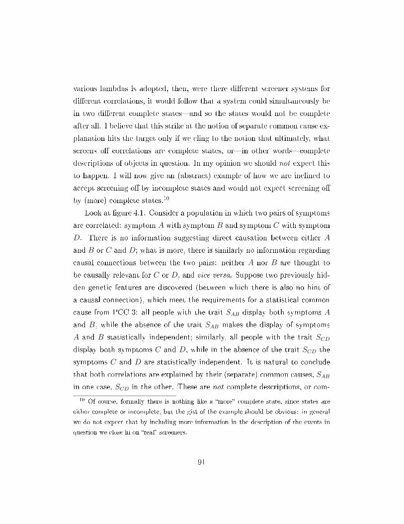
various lambdas is adopted, then, were there dierent screener systems for
dierent correlations, it would follow that a system could simultaneously be
in two dierent complete statesand so the states would not be complete
after all. I believe that this strike at the notion of separate common cause ex-
planation hits the target only if we cling to the notion that ultimately, what
screens o correlations are complete states, orin other wordscomplete
descriptions of objects in question. In my opinion we should not expect this
to happen. I will now give an (abstract) example of how we are inclined to
accept screening o by incomplete states and would not expect screening o
by (more) complete states.10
Look at gure 4.1. Consider a population in which two pairs of symptoms
are correlated: symptom A with symptom B and symptom C with symptom
D. There is no information suggesting direct causation between either A
and B or C and D; what is more, there is similarly no information regarding
causal connections between the two pairs: neither A nor B are thought to
be causally relevant for C or D, and vice versa. Suppose two previously hid-
den genetic features are discovered (between which there is also no hint of
a causal connection), which meet the requirements for a statistical common
cause from PCC 3: all people with the trait SAB display both symptoms A
and B, while the absence of the trait SAB makes the display of symptoms
A and B statistically independent; similarly, all people with the trait SCD
display both symptoms C and D, while in the absence of the trait SCD the
symptoms C and D are statistically independent. It is natural to conclude
that both correlations are explained by their (separate) common causes, SAB
in one case, SCD in the other. These are not complete descriptions, or com-
10 Of course, formally there is nothing like a more complete state, since states are
either complete or incomplete, but the gist of the example should be obvious: in general
we do not expect that by including more information in the description of the events in
question we close in on real screeners.
91

plete states; suppose for clarity that other predicates are excluded and the
individuals are to be described by means of possession (or lack) of the two
genetic traits in question. Then, a complete state would be a Boolean com-
bination of SAB and SCD, but we would have no reason at all to expect any
such combination to screen o both correlations.
92
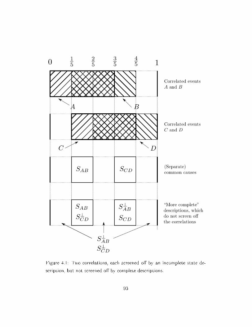
Figure 4.1: Two correlations, each screened o by an incomplete state de-
scription, but not screened o by complete descriptions.
93

4.7 Exploiting the detection loophole
In a given run of any experiment similar to the one described at the beginning
of this chapter, it may happen that only one detector res, or even none of
them does. The detectors are inecient. This may be attributed simply to
random errors of the experimental equipment, but one could also entertain
the thought that the ineciency is due to a hidden property of the emitted
particles. This is the central idea behind the so called Prism models (dating
back to Fine (1982b)).
A model of this kind is given by a meticulous construction in Szabó & Fine
(2002). The hidden variable may take one of 48 values. It is deterministic
in the sense that each value of the hidden variable predetermines whether
the given particle will be detected by the detector and, if this happens, what
the measurement result will be. Experimental probabilities are recovered.
The main trick is a sort of unfair sampling, introduced so that the detected
particles violate Bell-CH inequalities.
Since the model is deterministic, factorisability (and a fortiori OI) has
to hold in it. However, such models are understandably generally considered
ad hoc (Shimony (2009)) and, with the increasing eciency of detectors,
methods were proposed for closing the detection loophole (see again Shimony
(2009)).
4.8 Common causes as hypersurfaces
Lastly, let us briey mention another PCC-related option present in the
literature. Up to now, both in the big space and small space approach, the
supposed common causes for Bell-type correlations were events in probability
spaces. Buttereld (2007) describes in detail a view (developed rst in But-
tereld (1989)) called Stochastic Einstein Locality (SEL), in which common
94
causes are factors which determine probabilities of events (while nothing is
said about the probabilities of the factors themselves). For an event E (asso-
ciated with a space-time region), any hypersurface cutting through E's past
light cone C−(E) determines a probability, Pt(E), of E's occurrence.
The author discusses a few formulations of the SEL idea and provides
proofs of their formal relations. In one version, if E and F are space-like
related events (none is in either past- or future light cone of the other) and
t is a hypersurface cutting through(C−(E) ∪ C−(F )
)\(C−(E) ∩ C−(F )
),
then
Pt(E ∧ F ) = Pt(E) · Pt(F ).11
The similarity with the screening o condition is obvious; it is just that the
screener is in the subscript. SEL is also taken to be violated by violations
of Bell inequalities. The conceptual dierence between SEL and PCC is
that while PCC (at least in its more formal shapes, like PCC 3) is plausibly
falsied by everyday examples (sea levels / bread prices etc.), it takes a
Bell-type experimental setting to violate SEL.
4.9 Summary
The violation of Bell inequalities has an impact on these formulations of PCC
which require screening o. If the only candidates for common causes in this
case are complete states of the source on emission, thenif they are not
statistically relevant for the choices of detector settings and they in turn are
not statistically relevant for the measurement results in the other wingthe
common causes cannot act as screeners, thus violating the rst condition in
the denition of a statistical common cause. This is one of the motivations
for abandoning the general requirement of screening o from the denition
11 We omit the subscript referring to a possible world.
95

of common causes, even if one would like to preserve Reichenbach's idea that
common causes for correlations should exist (i.e. PCC 1)). The motivation is
similar to the one given in arguments from conservation principles (see e.g.
chapter 6 of Cartwright (1989) and section 2.4.1 of the current essay). Recent
results by Portmann & Wüthrich (2007) and Hofer-Szabó (2010) show that
the additional caution gained by the move from assuming common common
causes to assuming separate common causes for the various correlations is not
enough to block derivations of empirically falsiable Bell-type derivations.
96

Chapter 5
The Principle of the Common
Cause and the Causal Markov
Condition
A big part of modern probabilistic causality is concerned with the task of
causal modelingthat is, deriving causal information from statistical data
and depicting causal structures by means of graphs (usually directed acyclic
graphs, or DAGs; denitions will follow). The graphs are frequently called
Bayesian networks1. We have all heard the slogan that correlation does
not mean causation; it would be a trivialization, but perhaps an illustrative
one, to say that the Bayesian networks project begins with a contraposition
of causation means correlation: independence means absence of (direct)
causation. From statistical data information about independence (and con-
ditional independence) of variables is gathered, and on that basis a DAG is
constructed with the variables as nodes and arrows denoting direct causal
relationship (according to one of many algorithms available; see Spirtes et al.
1 Not because the interpretation of the probability is Bayesian, but because of the use
of Bayes' theorem for updating probabilities.
97

(2000) and Williamson (2005) for the adding arrows algorithm).
There is a condition, called the Causal Markov condition (henceforth
usually CMC), which is frequently taken as one which a pair consisting of a
DAG and a probability distribution for the values of its nodes should satisfy
if the pair is to be admitted as reliably depicting a real causal situation. One
of the most important books for the whole movement, Pearl (2000), cites the
Principle of the Common Cause as one of two sources of inspiration for the
condition (which will be discussed below). Later on, it seemed to have become
common knowledge that the PCC follows from the CMC; proofs of this fact
are given e.g. by Williamson (2005) and Arntzenius (2005), while Eberhardt
(2009) states that Reichenbach's principle of common cause is a special
case of the causal Markov condition when taken to apply to distributional
properties. It is therefore quite surprising that one of the most distinguished
writers on the subject, Clark Glymour, claims in a recent paper (Glymour
(2010)) that Neither, contrary to many commentators, does it [the CMC]
imply Reichenbach's Principle of the Common Cause (p. 175). Are all the
proofs wrong, then? Or is the principle they refer to something dierent from
Reichenbach's PCC? The issue is important, since if the implication holds,
then any argument against the PCC is dangerous for the CMC, too. We
will study this question in this chapter by providing the needed denitions
(the presentation will be based mainly on Spirtes et al. (2000)), discussing
the philosophical relationship between the CMC and PCC, and presenting
a proof regarding the CMC/PCC relationship. While the proof is based on
Williamson (2005) (p. 52), we will present it in a dierent way, to highlight
the fact the main idea can be expressed without reference to any causal
concepts.
98

5.1 DAGsan introduction
Let us start with the required denitions. A directed graph G over V is a
pair 〈V,E〉, where V is a set of nodes and E a set of arrows (ordered pairs
of nodes). A path between nodes X and Y is a sequence of nodes beginning
with X and ending with Y such that for any two nodes adjacent in the
sequence there is an arrow between them (the direction does not matter).
A node X on a path is a collider if together with its adjacent nodes Y and
Z in the path it forms an inverted fork: Y → X ← Z. There is a directed
path between vertices X and Y , a fact symbolized by X Y , if there is
an arrow between X and Y (X → Y ) or there is some node Z such that
X Z and Z → Y . A directed graph is acyclic if for any node X it is not
true that X X. We will always assume that the nodes of any given graph
represent random variables.
Par(X), the set of parents of a node X, consists of the nodes Z such
that Z → X. Childr(X), the set ofX's children, includes exactly the nodes
Z such that X → Z. The sets Anc(X) (ancestors) and Desc(X) (descen-
dants) are dened by substituting for → in the last two sentences
but with the addition that a node always is its own ancestor and descendant,
but never its child or parent (see Spirtes et al. (2000), p. 10).
Not to stray from the recent literature, we will express the fact that
variables X and Y are independent2 as X |= Y ; that they are independent
given a third variable Z as X |= Y | Z; and that they are not independent
as X Y .
The Markov Condition, in contrast to the Causal Markov Condition, is
expressed exclusively by means of probabilistic and graph-related notions. It
does not concern DAGs per se, but DAGs together with probability distri-
butions over the set of their nodes.
2 See denition 5 in chapter 2, p. 7.
99

Denition 13 [Markov Condition] A DAG G over V and a probability
distribution P (V) satisfy the Markov Condition if and only if for anyW ∈ V,
W |= V \(Desc(W ) ∪ Par(W )
)| Par(W ).
In other words, in a graph which (together with a probability distribution
over the set of its nodes) satises the Markov Condition (MC), every variable
is independent of its nondescendants conditional on its parents. It is also
independent (again, conditional on its parents) of its ancestors which are not
its parents.
The MC can hold of DAGs and probability distributions with no appeal
to any causality whatsoever. The Causal Markov Condition (CMC) holds of
a subset of graph-probability distribution pairs for which MC holds; namely
the graphs have to be causal: they should represent a causal structure and
the distribution to be generated by that structure. A causal structure for
a population is a set of variables V together with a set E of ordered pairs
of these variables, where a pair 〈X, Y 〉 belongs to E whenever X is a direct
cause3 of Y relative to V4 (Spirtes et al. (2000), p. 22). Suppose we have a
causal structure C = 〈V,E, 〉 and P (V) is the actual probability distribution
over V; we then say that the distribution P (V) is generated by the causal
structure C. A causal structure 〈V,E〉 is causally sucient for a given
population i it contains all common causes of any two variables in V, apart
from the ones which have the same value for all elements of the population.
It is interesting that the denition of causal representation (Spirtes et al.
3 It is interesting that the denition of a variable X being a direct cause of variable Y
is in this framework a counterfactual denition; see Spirtes et al. (2000), p. 20.4 This last qualication is importantif X causes Z by means of an intermediary
variable Y , and yet we exclude Y from our causal structure, then even though X is not a
direct cause of Z in general, we should have the pair 〈X,Z〉 in the set of pairs being the
second element of our causal structure.
100
(2000), p. 24) explicitly refers only to graphs representing causally sucient
causal structures; a DAG G = 〈V,E〉 represents a causally sucient causal
structure C = 〈W,F〉 if each node from V represents a variable from W,
every variable from W is represented by some variable from V, and there
is an arrow between two vertices from V if and only if the ordered pair
consisting of the two variables represented by the nodes at the rear end and
the head of the arrow belongs to F. A causal graph is then dened as a DAG
which represents a causal structure (Spirtes et al. (2000), p. 24).5
We take the quoted part of the denition of a causal graph to mean a
causally sucient structure, since working on such structures seems to be
the overall goal. The reasons are obvious; e.g., should one ignore a common
cause C for two correlated (but really directly causally unrelated) variables
A and B, one would be tempted to draw A → B or B → A in the
causal graph, which would then give an incorrect picture of the real causal
structure. Of course, it may be by no means evident what the real common
causes are, and, a fortiori, which variables should be included for the causal
structure to be sucient. Nevertheless, we take causal graphs to be graphs
representing causally sucient structures; this decision will have no impact
on the conclusions of this chapter.
5.2 The Causal Markov Condition
Denition 14 [Causal Markov Condition] A DAG G over V and a
probability distribution P (V) satisfy the Causal Markov Condition if and
only if
5 In fact, it does not seem that any signicant generality is lost if a causal graph is
thought to be coextensive with the structure it represents; in other words, if we can think
of causal graphs simply being causal structures, and of its nodes being variables.
101

• G is a causal graph;
• P (V) is generated by the structure represented by G;
• G and P (V) satisfy the Markov Condition.
What is the relationship of the CMC and the principle of the common
cause, e.g. in the PCC 2 version, reformulated so that it would refer to
random variables, and generalized so that the correlation would require the
existence of a set of common causes?6 Suppose there are only two vari-
ables in the causal structure, X and Y . If they constitute a real-life coun-
terexample to the PCCthat is, they are correlated, but there are no di-
rect causal relations between them and there is in the world no set of vari-
ables which would render them conditionally independentthen the struc-
ture C := 〈X, Y , ∅〉 is causally sucient for the given population. There-
fore the graph G := 〈X, Y , ∅〉, with two vertices but no arrows7, is of
course a causal graph, but together with the real distribution over X and Y ,
according to which X and Y are correlated, of course fail to meet the Markov
Condition (X is not independent of Y conditional on the empty set), and so
a fortiori the Causal Markov Condition.
In the other direction, suppose PCC 2 (in the reformulation hinted at
above) is generally true, and that a causally sucient structure is consid-
ered. The exogenous variables8 have to be pairwise independent, since if
they were not, then some of them would have to have (common) causes, and
6 See Gyenis & Rédei (2010) for a rigorous translation of Reichenbach's ideas to the
language of random variables; we will return to these matters at the end of chapter 6.7 Again, the X in the graph is a node which represents the X, a variable in the
structure.8 Meaning, the ones which are not pointed to by any arrow; the variables which have no
causes in the structure considered. Such variables have to exist if the plausible assumption
of nitude of the causal structure (we can only measure a nite number of variables and
102
so some of them would not be exogenous after all. It is a well known fact
(for a proof see e.g. Steel (2005)) that the MC is true in any graph with
independent exogenous variables. However, a stronger independence then
pairwise independence is needed: due to the so called Bernstein Paradox,
there might be a dependence between sets of variables even if there is no de-
pendence between any two variables9. Therefore, to arrive at an implication
from PCC to the CMC, one would have to reformulate the principle not only
so that it considered random variables and more than one common cause, but
also generalized the starting point from the correlation of two variables to the
existence of a correlated set of variables (with no direct causal relationships).
We would like to show that some arguments oered in the literature as
proving some version of the PCC on the basis of CMC can be expressed
without reference to any causal notions. For example, the following principle
is called by Williamson (2005) a Principle of the Common Cause.
Denition 15 [Principle of the Common Ancestor] The Principle of the
Common Ancestor holds of a DAG G over V and a probability distribution
P (V) if, whenever A B, then A B or B A or there is a U ⊆ V such
that C ∈ U implies C A and C B, and A |= B | U .
The shortest (known to us) proof of the relationship between the Markov
Condition and the Principle of the Common Ancestor uses the notion of
d-separation (Pearl (1988); we use the denition from Spirtes et al. (2000),
p. 14). (The d is from directional; the notion of d-separation is highly tech-
nical and not easy to illustrate intuitivelysee e.g. chapter 3.7.1 of Spirtes
et al. (2000).) Consider a graph G. If X and Y are distinct vertices of G
and W is a set of vertices of G containing neither X nor Y , then X and Y
adding an innite number of unmeasured variables to the given structure would require
some serious argument) is made, due to the fact that the graphs are to be acyclic.9 For a discussion of this paradox in the context of common causes, see Unk (1999).
103

are d-separated given W (W d-separates X and Y ) in G if and only if there
exists no path U between X and Y such that
• every collider on U has a descendant in W;
• no other vertex on U belong to W.
The notion of d-separation is very useful when discussing Bayesian net-
works due e.g. to the following fact, which we will need later on (we cite here
the formulation from Williamson (2005), p. 17):
Fact 7 (Verma & Pearl (1988)) Given a DAG G over V and R, S, T ⊆V, T d-separates R and S if and only if R |= S | T for all probability
distributions P (V) which together with G satisfy the Markov Condition.
For example, if we know that a DAG with a probability distribution
satises the Markov condition, and we nd that distinct variables X and Y
are d-separated by ∅, we can infer that X and Y are not correlated.
The following fact is a direct companion to Proposition 4.1 from
Williamson (2005), p. 52; it has (together with the proof) been only reworded
so that it does not refer to causal notions.
Fact 8 The Markov Condition implies the Principle of the Common Ances-
tor.
Proof: Suppose the Markov Condition holds of a graph G over V and
a probability distribution P (V). Let A,B ∈ V. Suppose it is not the case
that (A B or B A or there is a C ∈ V such that C A and C B).
Then variables A and B are d-separated by ∅, since any path between them
has to include a collider. In such a case, A |= B.Suppose, then, that A B. From the last paragraph we infer by contra-
position that, if it is not the case that A B or B A (when the Principle
104

would be trivially true), there has to be at least one C ∈ V such that C A
and C B. Let U be the set of all such Cs. U d-separates A and B, so
A |= B | U.
Of course, if the graph under consideration is causal, the Principle of the
Common Ancestor becomes a version of PCC, claiming the existence of a
set of common causes for the correlated variables, which act as screeners for
those variables.
5.3 Conclusions
We have seen that real-life counterexamples to PCC would lead to failure
of CMC. We have also presented a general proof that in any graph which
satises MC a certain principle is valid; if the graph is a causal graph (and
the distribution is the one generated by the structure), then this principle be-
comes a version of PCC. What is, then, the reason for the already mentioned
claim of Glymour (2010) that Reichenbach's PCC does not follow from the
CMC?
Perhaps the matter is simple and the word Reichenbach is the key;
notice the complete absence of the statistical relevance conditions from the
considerations of these chapter. This is of course reasonable; if we speak
about correlated events, we can consider a cause raising the probability of
the events; but the correlation of two variables (e.g. X and Y ) typically leads
to numerous correlations between events (e.g. X = 1 and Y = 1 and so
on, for various (but maybe not all) values of the variables). But let us con-
sider two correlated binary variables10, which do not inuence each other
directly. One can look at the existence of a common cause variable for such
two variables as the existence of a common screener o for the correlations
10 Recall the close correspondence between binary variables and events, section 2.1, p. 7
above.
105

between the appropriate events. But, as we know from example 2 in section
3.2, it might very well be that no element of the screener o is positively
statistically relevant for any of the correlated events, so Reichenbach's con-
ditions (even as generalized as in the denition of a statistical common cause
system) cannot be satised.
106

Chapter 6
Causal closedness
The material in sections 6.1-6.5 originates from joint research by Michaª
Marczyk and the author, gathered in Marczyk & Wro«ski (2010).
6.0.1 A preliminary formal remark
For the majority of the results of this chapter, the sample spaces of the prob-
ability spaces involved are irrelevant. The crucial factors are the Boolean
algebra being the event space and the measure dened on that algebra.
Thereforeuntil section 6.9if no other qualication is given, a probability
space is meant to be a pair 〈S, P 〉, where S is a Boolean algebra1 and P is a
classical measure on S. In section 6.5 nonclassical spaces are considered, in
which the Boolean algebra is exchanged for a nondistributive orthomodular
lattice. The required denitions are presented.
Also, throughout this chapter, by a common cause we always mean a
statistical common cause. At the beginning we usually supply the addi-
tional adjective, but then sometimes refrain from using it to conserve space,
1 We omit the usual requirement of σ-completeness because, while the notion of causal
up-to-n-closedness will be general, the results proved regarding it will concern the nite
cases only.
107
as the arguments unfortunately become rather cluttered even without the
additional vocabulary.
6.1 Causal (up-to-n-)closedness
6.1.1 Introduction
Suppose a probability space contains a correlation between two events we
believe to be causally independent. Does the space contain a common cause
for the correlation? If not, can the probability space be extended to contain
such a cause but `preserving' the old measure? This question has been asked
and answered in the positive in Hofer-Szabó, Rédei & Szabó (1999), where
the notion of common cause completability was introduced: speaking a bit
informally, a probability space S is said to be common cause completable
with respect to a set A of pairs of correlated events i there exists an exten-
sion of the space containing statistical common causes of all the correlated
pairs in A. Gyenis and Rédei (2004) introduced the notion of common cause
closedness, which (in our slightly dierent terminology) is equivalent to the
following: a probability space S is common cause closed (or causally closed)
with respect to a relation of independence Rind ⊆ S2 i it contains statistical
common causes (recall denition 9, p. 53) for all pairs of correlated events
belonging to Rind. The authors have proven therein that a nite classical
probability space with no atoms of probability 0 is non-trivially common
cause closed w.r.t. the relation of logical independence i it is the space
consisting of a Boolean algebra with 5 atoms and the uniform probability
measure.2 In other words, nite classical probability spaces (big enough to
2 The phrasing of the paper was in fact stronger, omitting the assumption about non-
0 probabilities on the atoms (due to a missed special sub-case in the proof of case 3 of
proposition 4 on p. 1299). The issue is connected to the distinction between proper and
improper common causes and is discussed below in section 6.3.
108

contain correlations between logically independent events) are in general not
common cause closed w.r.t. the relation of logical independence, i.e. they
contain a correlation between logically independent events for which no sta-
tistical common cause in the space exists; the only exception to this rule is the
space with precisely 5 atoms of probability 15each. More spaces are common
cause closed w.r.t. a more stringent relation of logical independence modulo
measure zero event (L+ind, see denition 17 below): they are the spaces with
5 atoms of probability 15each and any number of atoms of probability 0.
Still, a (statistical) common cause is not the only entity which could
be used as an explanation for a correlation. As we mentioned earlier in
chapter 3, Hofer-Szabó and Rédei (2004) generalized the idea of a statistical
common cause, arriving at statistical common cause systems (SCCSs; recall
denition 10, p. 53). As already noted, SCCSs may have any countable size
greater than 1; the special case of size 2 reduces to the usual notion of
common cause.
It was natural for corresponding notions of causal closedness to be intro-
duced; a probability space is said to be causally n-closed3 w.r.t. a relation
of independence Rind i it contains an SCCS of size n for any correlation
between A,B such that 〈A,B〉 ∈ Rind. It is one of the results of the present
chapter that with the exception of the 5-atom uniform distribution probabili-
ty space, no nite probability spaces without 0 probability atoms are causally
n-closed w.r.t. the relation of logical independence, for any n > 2. Similarly,
with the exception of the spaces with 5 atoms of probability 15each and
any number of atoms of probability 0, no nite probability spaces with 0
probability atoms are causally n-closed w.r.t. L+ind, for any n > 2.
We are interested in a slightly dierent version of causal closedness. If the
overarching goal is to nd explanations for correlations, why should we expect
all explanations to be SCCSs of the same size? Perhaps some correlations
3 The notion was introduced in Hofer-Szabó & Rédei (2006).
109
are explained by common causes and other by SCCSs of a bigger size. We
propose to explore the idea of causal up-to-n-closednessa probability space
is causally up-to-n-closed w.r.t. a relation of independence Rind i it contains
an SCCS of size at most n for any correlation between events A,B such that
〈A,B〉 ∈ Rind.
It turns out that, in the class of nite classical probability spaces with
no atoms of probability 0, just as the space with 5 atoms and the uniform
measure is unique with regard to common cause closedness, the whole class
of spaces with uniform distribution is special with regard to causal up-to-3-
closednesssee theorem 4: a nite classical probability space with no atoms
of probability 0 has the uniform distribution i it is causally up-to-3-closed
w.r.t. the relation of logical independence. We provide a method of con-
structing a statistical common cause or an SCCS of size 3 for any correlation
between logically independent events in any nite classical probability space
with the uniform distribution.
We require (following Gyenis and Rédei) of a causally closed probability
space that all correlations be explained by means of properthat is, diering
from both correlated events by a non-zero measure eventstatistical common
causes. This results in the fact that a space causally closed w.r.t. the relation
of logical independence can be transformed into a space which is not causally
closed w.r.t. this relation just by adding a 0-probability atom. Perhaps,
to avoid this unfortunate consequence, the notion of logical independence
modulo measure zero event should be required? We discuss the matter in
section 6.3.
In this chapter we also briey consider other independence relations, a
generalization of our results to nite non-classical probability spaces, and
closedness w.r.t. to the more general deductive explanantes. Lastly, we briey
report some known results on causal closedness of atomless spaces we will
use in the next chapter.
110

6.1.2 Preliminary denitions
In the following assume that we are given a nite classical probability space
〈S, P 〉, where S is a nite Boolean algebra and P is a classical measure on S.
By Stone's representation theorem, S is isomorphicand may be identied
withthe algebra of all subsets of the set 0, . . . , n− 1 for some n ∈ N.In the sequel we will sometimes consider spaces of the form 〈S+, P+〉,
where S+ and P+ are as dened below:
Denition 16 Let 〈S, P 〉 be a nite classical probability space. S+ is the
subalgebra of S containing all and only the non-zero probability atoms of S.
P+ is the restriction of P to S+.
We will now dene two relations of logical independence. Intuitively, we
will regard two events as logically independent if, when we learn that one of
the events occurs (or does not occur), we cannot infer that the other occurs
(or does not occur), for all four Boolean combinations.
Denition 17 [Logical independence] We say that events A,B ∈ S are
logically independent (〈A,B〉 ∈ Lind) i all of the following sets are nonempty:
• A ∩B;
• A ∩B⊥;
• A⊥ ∩B;
• A⊥ ∩B⊥.
We say that events A,B ∈ S are logically independent modulo measure
zero event (〈A,B〉 ∈ L+ind) i all of the following numbers are positive:
• P (A ∩B);
• P (A ∩B⊥);
111
• P (A⊥ ∩B);
• P (A⊥ ∩B⊥).
Equivalently, two events are logically independent if neither of the events
is contained in the other one, their intersection is non-empty and the sum of
the two is less than the whole space. Two events are logically independent
modulo measure zero event if every Boolean combination of them has a non-
zero probability of occurring. It is always true that L+ind ⊆ Lind; if there are
0-probability atoms in the space, the inclusion may be strict.
The following denition is a renement of the SCC idea, expressing the
requirement that a common cause should be meaningfully dierent from both
correlated events.
Denition 18 [Proper SCC(S)] A statistical common cause C of events
A and B is a proper statistical common cause of A and B if it diers from
both A and B by more than a measure zero event. It is an improper SCC of
these events otherwise.
An SCCS Cii∈I of events A and B is a proper SCCS of A and B if all
its elements dier from both A and B by more than a measure zero event.
It is an improper SCCS of these events otherwise.
We will sometimes say that a probability space contains an SCCS, which
means that the SCCS is a partition of unity of the underlying algebra of the
space.
We now come to the concept being the main topic of this chapter. Should
someone prefer it, the following denition could be phrased in terms of SCCSs
only.
112

Denition 19 [Causal up-to-n-closedness] We say that a classical prob-
ability space is causally up-to-n-closed w.r.t. to a relation of independence
Rind if all pairs of correlated events independent in the sense of Rind possess a
proper statistical common cause or a proper statistical common cause system
of size at most n.
If the space is causally up-to-2-closed, we also say that it is causally closed
or common cause closed.
6.1.3 Summary of the results of this chapter
〈S, P 〉 isup-to-3-closed
w.r.t.
Lind L+ind
P is uniform ⇒ (9) ⇒ (9)
⇐ (10)P+ is uniform ⇒∗ (11) ⇔ (10,11)
Table 6.1: The main results of the chapter. The numbers in parentheses
correspond to lemmas below.
Theorem 3 will be our main tool in proving the lemmas featured in table
6.1.
Theorem 3 Let 〈S, P 〉 be a nite classical probability space with S+ having
at least 4 atoms of non-zero probability. Then P+ is uniform if and only if
〈S+, P+〉 is causally up-to-3-closed w.r.t. L+ind.
Lemmas 9-11 tie uniformity of P and P+ with causal up-to-3-closedness
of 〈S, P 〉 with respect to the two notions of independence introduced above.
113

Lemma 9 Let 〈S, P 〉 be a nite classical probability space with S having at
least 4 atoms. If P is uniform, then 〈S, P 〉 is causally up-to-3-closed w.r.t.
Lind and L+ind.
Lemma 10 Let 〈S, P 〉 be a nite classical probability space with S+ having
at least 4 atoms. If P+ is not uniform, then 〈S, P 〉 is not causally up-to-3-
closed w.r.t. either Lind or L+ind.
Lemma 11 Let 〈S, P 〉 be a nite classical probability space with S+ having
at least 4 atoms. If P+ is uniform, then 〈S, P 〉 is causally up-to-3-closed
w.r.t. L+ind. All correlated pairs from Lind \ L+
ind have statistical common
causes, but some only have improper ones.
6.2 Proofs
6.2.1 Some useful parameters
For expository reasons, we will not prove theorem 3 directly, but rather show
its equivalent, theorem 4 (p. 115). Before proceeding with the proof, we shall
introduce a few useful parameters one may associate with a pair of events A,
B in a nite classical probability space 〈S, P 〉.Let n be the number of atoms in the Boolean algebra S. The size of
the set of atoms lying below A in the lattice ordering of S will from now
on be referred to as a, and likewise for B and b. The analogous parameter
associated with the conjunction of events A and B is just the size of the
intersection of the relevant sets of atoms and will be called k.
It will soon become apparent that while a and b have some utility in the
discussion to follow, the more convenient parameters describe A and B in
terms of the number of atoms belonging to one, but not the other. Thus we
let a′ = a − k and b′ = b − k. In fact, if we set z = n − (a′ + k + b′), we
114
obtain a set of four numbers precisely describing the blocks of the partition
of the set of atoms of S into the four classes which need to be non-empty for
A and B to be logically independent. It is clear that in the case of logically
independent events a′, b′, k and z are all non-zero.
Lastly, before we begin the proof of the main result of this chapter, let
us recall corollary 4, p. 59: when searching for statistical common causes,
screening o is enough. If both an event and its complement screen o a
correlation, then one of them is a statistical common cause for the correlation.
6.2.2 Proof of theorem 3
In this section we will provide a proof of the main tool in this chapter
theorem 3, formulated in section 6.1.3. The form in which it was stated in
that section is dictated by its use in the proofs of lemmas 9-11. However,
when treated in isolation, it is better versed in the following way:
Theorem 4 (Marczyk & Wro«ski (2010), equivalent to theorem 3)
Let 〈S, P 〉 be a nite classical probability space with no atoms of probability
0. Suppose S has at least 4 atoms.4 The following conditions are equivalent:
Measure uniformity: P is the uniform probability measure on S;
Causal up-to-3-closedness w.r.t. Lind: 〈S, P 〉 is causally up-to-3-closed
w.r.t. the relation of logical independence.
Before proceeding with the proof we will provide a sketch of the con-
struction and some requisite denitions. Instead of focusing on a particular
n-atom algebra, we will show how the problem presents itself while we `move'
4 It is easy to verify that if S has 3 atoms or less, then 〈S, P 〉 contains no correlations
between logically independent events.
115
from smaller to bigger algebras. We assume without loss of generality that
the set of atoms of an n-atom Boolean algebra is 0, 1, · · · , n− 1 and that
each event is a set of atoms. Consider the sequence of all nite classical prob-
ability spaces with the uniform probability measure, in which the number of
atoms of the underlying Boolean algebra of the space increases by 1 at each
step, beginning with the algebra with a single atom. We use the shorthand
expression at stage n to mean in the probability space with uniform dis-
tribution whose underlying Boolean algebra has n atoms. Observe that due
to our convention whereby events are identied with sets of atoms, an event
present at stage m (one found in the algebra from that stage) is also present
at all further stages. In other words, a set of atoms dening an event at
stage m can also be interpreted as dening an event at any stage m′, with
m′ > m. Thus we can naturally say that a certain event belongs to many
dierent probability spaces; e.g. the event 1, 2, 11 is present at stages 12,
13, and so on. Similarly, pairs of events can be present at many stagesand
be correlated at some, but not at others. If they are correlated at stage m,
they are correlated at all stages n, for n > m (see below). The same is true of
logical independence: a pair may not consist of logically independent events
at stage n, because their union is the whole set of n atoms, but may become
a pair of logically independent events at stage n+1, when an additional atom
is introduced, which does not belong to either of the events in question.
Some remarks on the shape of events considered are in order. We will al-
ways be talking about pairs of eventsA,B, with numbers a, a′, b, b′, k, z and n
dened as above (see section 6.2.1). We assume a > b. Also, since we are deal-
ing with the uniform measure, all relevant characteristics of a pair of events
A,B are determined by the numbers a′, b′, k, and z; therefore, for any combi-
nation of these numbers it is sucient only to consider a single example of a
pair displaying them. The rest is just a matter of renaming the atoms. For ex-
ample, if we are looking for an explanation for the pair 8, 7, 3, 5, 2, 8, 7
116

at stage 10, or the pair 1, 3, 5, 6, 1, 6, 4 at the same stage, we shall
search for an explanation for the pair 0, 1, 2, 3, 2, 3, 4 at stage 10 and
then just appropriately `translate' the result (explicit examples of this follow
in section 6.2.2). In general: the convention we adopt is for A to be a set
of consecutive atoms beginning with 0, and B a set of consecutive atoms
beginning with a− k.
For illustrative purposes we propose to examine the situation at the early
stages. The proof proper begins with denition 20 below. For the remainder
of section 6.2.2, by common cause we will always mean proper common
cause; similarly with common cause system.
There are no correlated pairs of logically independent events at stage 1;
similarly for stages 2, 3 and 4. (Remember the measure is uniform and so at
stage 4 e.g. the pair 0, 1, 1, 2, while composed of logically independent
events, is not correlated.)
First correlated pairs of logically independent events appear at stage 5.
These are of one of the two following types: either a′ = b′ = k = 1, or
a′ = b′ = 1 and k = 2. Proposition 3 from Gyenis & Rédei (2004) says that
all pairs of these types have statistical common causes at stage 5. As noted
above, we can without loss of generality consider just two tokens of these
typesthe pairs 0, 1, 1, 2 and 0, 1, 2, 1, 2, 3. In the rst case,
the events already formed a logically independent pair at stage 4, but were
not correlatedwe will say that the pair appears from below at stage 5 (see
denition 20 below). In the second case, stage 5 is the rst stage where the
events form a logically independent pair, and they are already correlated at
that stage. We will say that the pair 0, 1, 2, 1, 2, 3 appears from above
at stage 5. There are no other correlated pairs of logically independent events
at stage 5. It will turn out that we can always nd statistical common causes
for pairs which appear from above or from below at a given stage.
117

Let us move to stage 6. A new (type of) pair appears from above
0, 1, 2, 3, 1, 2, 3, 4. No pairs appear from below, but both pairs which
appeared at stage 5 are still correlated and logically independent at stage 6
(as well as at all later stages), so they are again in need of an explanation at
this higher stage. It turns out that if a correlated pair of logically independent
events at stage n is `inherited' from the earlier stages, i.e. it appears neither
from above nor from below at stage n, we can modify the common cause
which we know how to supply for it at the stage where it originally appeared
to provide it with an explanation adequate at stage n. This takes the form
of a statistical common cause or, in some cases, an SCCS of size 3.
Denition 20 [Appearing from above or below] A pair A,B of eventsappears from above at stage n if it is (1) logically independent at stage n, (2)
not logically independent at stage n− 1 and (3) correlated at stage n.
A pair A,B of events appears from below at stage n if it is (1) logically
independent at stage n, (2) logically independent at stage n − 1 and (3)
correlated at stage n, but (4) not correlated at stage n− 1.
We will divide common causes into types depending on whether the occur-
rence of a given common cause makes the occurrence of at least one member
of the correlation it explains necessary, impossible or possible with probabil-
ity less then 1.5
Denition 21 [1-, 0-, and #-type statistical common causes] A proper
statistical common cause C for a correlated pair of logically independent
events A,B is said to be:
• 1-type i P (A | C) = 1 or P (B | C) = 1;
• 0-type i P (A | C⊥) = 0 or P (B | C⊥) = 0;
5 Since the context of theorem 4 is that of nite spaces, the dierence between necessity
and probability 1 can be dismissed.
118
• #-type i it is neither 1-type nor 0-type.
Notice that no statistical common cause C for some two logically inde-
pendent, correlated events A and B can be both 1-type and 0-type at the
same time.
Denition 22 [0-type statistical common cause system] A proper sta-
tistical common cause system of size n Cii∈0,...,n−1 is a 0-type statistical
common cause system (0-type SCCS ) for the correlation i P (A | Cn−1) = 0
or P (B | Cn−1) = 0.
We do not need to worry about the fact that rearranging the elements
of a 0-type SCCS necessarily make it lose the 0-type status, because during
the proof the SCCSs will be explicitly construed so that their last element
gives conditional probability 0 to both correlated events to be explained.
Were this notion to be used in general, its denition should be rephrased as
an existential condition: there exists m 6 n − 1 such that P (A | Cm) = 0
and P (B | Cm) = 0.
We will prove the following:
• if a pair appears from above at stage n, it has a statistical common
cause at that stage (lemma 13);
• if a pair appears from below at stage n, it has a statistical common
cause at that stage (lemma 14);
• if a pair of logically independent events is correlated at stage n and has
a statistical common cause or a 0-type SCCS of size 3 at that stage,
it has a statistical common cause or a 0-type SCCS of size 3 at stage
n+ 1 (lemma 15).
119
It should be straightforward to see that this is enough to prove theorem
4 (p. 115) in its `downward' direction. Consider a correlated pair of logically
independent events A,B at stage n. If it appears from above, we produce
a common cause using the technique described in lemma 13. If it appears
from below, we use the method from lemma 14. If it appears neither from
above nor from below, it means that it was logically independent at stage
n− 1 and was correlated at that stage, and we repeat the question at stage
n − 1. This descent terminates at the stage where our pair rst appeared,
which clearly must have been either from below or from above. This allows
us to apply either lemma 13 or lemma 14, as appropriate, followed by lemma
15 to move back up to stage n, where we will now be able to supply the pair
with an SCC or an SCCS of size 3. As said before, the SCCs and SCCSs we
will construct will always be proper SCCs and SCCSs.
Put Corr(A,B) := P (AB) − P (A)P (B). Corr(A,B) can always be
expressed as a fraction with the denominator being n2. Of special inter-
est to us will be the numerator of this fraction. Let us call this number
SCn(A,B). (For example, if A = 0, 1, 2 and B = 2, 3, SC5(A,B) = −1.)
If SCn(A,B) 6 0, the events are not correlated at stage n. If SCn(A,B) > 0,
A and B are correlated at stage n and we need to nd either a common cause
or a common cause system of size 3 for them. The following lemma will aid
us in our endeavour (remember the denitions from section 6.2.1):
Lemma 12 Let 〈Sn, P 〉 be a nite classical probability space, Sn being the
Boolean algebra with n atoms and P the uniform measure on Sn. Let A,B ∈Sn. Then SCn(A,B) = kz − a′b′.
Proof: Corr(A,B) = P (AB) − P (A)P (B) = kn− k+a′
nk+b′
n=
= k(n−k−a′−b′)−a′b′n2 = kz−a′b′
n2 . Therefore SCn(A,B) = kz − a′b′.
120

An immediate consequence of this lemma is that any pair of logically in-
dependent events will eventually (at a high enough stage) be correlated it is
just a matter of injecting enough atoms into z. For example, consider events
A = 0, 1, 2, 3, 4, 5, 6, B = 6, 7, 8, 9, 10, 11. At any stage n, SCn(A,B) is
equal to z− 30. This means that the pair is correlated at all stages in which
z > 30; in other words, at stages 43 and up. At some earlier stages (from
13 to 42) the pair is logically independent but not correlated; at stage 12 it
is not logically independent; and the events constituting it do not t in the
algebras from stages lower than that.
Notice that since for any A,B: SCn+1(A,B) = SCn(A,B) + k, it follows
that at the stage m where the pair rst appears (either from above or from
below) SCm(A,B) is positive but less than or equal to k.
We now have all tools we need to prove theorem 4.
Proof: (of theorem 4)
Measure uniformity⇒ Causal up-to-3-closedness w.r.t. Lind
Lemma 13 Suppose a pair A,B appears from above at stage n. Then there
exists a 1-type common cause for the correlation at that stage.
Proof: We are at stage n. Since the pair A,B appears from above
at this stage, z = 1 and so (by lemma 12) SCn(A,B) = k − a′b′. (If
z was equal to 0, the events would not be logically independent at stage
n; if it was greater than 1, the events would be logically independent at
stage n − 1 too, and so the pair would not appear from above at stage
n.) Notice that since A,B are logically independent (so both a′ and b′ are
non-zero) but correlated at stage n, 0 < SCn(A,B) = k − a′b′ < k. Let
C consist of exactly SCn(A,B) atoms from the intersection A ∩ B. Such
a C will be a screener-o for the correlation, since P (AB | C) = 1 =
121

P (A | C)P (B | C). What remains is to show that C⊥ is a screener-o as
well. This follows from the observation that P (AB | C⊥) = k−(k−a′b′)n−(k−a′b′) =
a′b′
n−k+a′b′= a′b′(n−k+a′b′)
(n−k+a′b′)2= a′b′(1+a′+b′+k)−a′b′k+a′2b′2
(n−k+a′b′)2= a′b′+a′b′2+a′2b′+a′2b′2
(n−k+a′b′)2=
a′+a′b′
n−k+a′b′· b′+a′b′
n−k+a′b′= k+a′−(k−a′b′)
n−k+a′b′· k+b′−(k−a′b′)
n−k+a′b′= k+a′−SCn(A,B)
n−k+a′b′· k+b′−SCn(A,B)
n−k+a′b′=
P (A | C⊥)P (B | C⊥).
Lemma 14 Suppose a pair A,B appears from below at stage n. Then there
exists a 1-type common cause or a 0-type common cause for the correlation
at that stage.
Proof:
Case 1: k > b′ and a′ > z.
In this case we will construct a 1-type common cause. Let C consist of
k−b′ atoms from A∩B and a′−z atoms from A\B. Since C ⊂ A, it screens o
the correlation: P (AB | C) = P (B | C) = 1 ·P (B | C) = P (A | C)P (B | C).
We need to show that C⊥ screens o the correlation as well. This follows from
the fact that P (AB | C⊥) = b′
n−(k−b′)−(a′−z) = b′
2b′+2z= 2b′2+2zb′
(2b′+2z)2= (b′+z)2b′
(2b′+2z)2=
b′+z2b′+2z
· 2b′
2b′+2z= b′+z
n−(k−b′)−(a′−z) ·2b′
n−(k−b′)−(a′−z) = P (A | C⊥)P (B | C⊥).
Case 2: z > b′ and a′ > k.
In this case we will construct a 0-type common cause. Let C⊥ consist of
a′ − k atoms from A \ B and z − b′ atoms from (A ∪ B)⊥. Since C⊥ ⊂ B⊥,
it screens o the correlation: P (AB | C⊥) = 0 = P (A | C⊥) · 0 = P (A |C⊥)P (B | C⊥). We need to show that C too screens o the correlation. This
follows from the fact that P (AB | C) = kn−(a′−k)−(z−b′) = k
2k+2b′= 2k2+2kb′
(2k+2b′)2=
2k(k+b′)(2k+2b′)2
= 2k2k+2b′
· k+b′
2k+2b′= 2k
n−(a′−k)−(z−b′) ·k+b′
n−(a′−k)−(z−b′) = P (A | C)P (B | C).
Case 3a: z > a′, k > a′ and a′ > b′.
As can be veried easily, in this case k = z = a′ and b′ = a′ − 1. We
can construct both a 0-type common cause and a 1-type common cause.
Suppose we choose to produce the former. An appropriate C⊥ would consist
122

of just a single atom from (A ∪ B)⊥; C⊥ screens o the correlation because
P (AB | C⊥) = 0 = P (A | C⊥)P (B | C⊥). That C is also a screener-
o is guaranteed by the fact that P (AB | C) − P (A | C)P (B | C) =k
k+a′+b′+z−1− k+a′
k+a′+b′+z−1· k+b′
k+a′+b′+z−1= k
4k−2− 2k
2(2k−1)· 2k−1
4k−2= 0.
To produce a 1-type common cause instead, let C consist of just a single
atom from (A ∩ B); C screens o the correlation because P (AB | C) =
1 = P (A | C)P (B | C). That C⊥ is also a screener-o follows from the
fact that P (AB | C⊥) = k−1k−1+a′+b′+z
= b′
2b′+2a′= 2b′2+2a′b′
(2b′+2a′)2= (a′+b′)2b′
(2b′+2a′)2=
a′+b′
2b′+2a′· 2b′
2b′+2a′= k−1+a′
2b′+2a′· k−1+b′
2b′+2a′= P (A | C⊥)P (B | C⊥).
Case 3b: z = a′ + 1 and k = a′ = b′.
In this case we will construct a 0-type common cause. Let C⊥ consist
of just a single atom from (A ∪ B)⊥; C⊥ screens o the correlation because
P (AB | C⊥) = 0 = P (A | C⊥)P (B | C⊥). C screens o the correlation
because P (AB | C) = k4k
= 4k2
16k2= 2k
4k· 2k
4k= k+a′
k+a′+b′+z−1· k+b′
k+a′+b′+z−1= P (A |
C)P (B | C).
Case 3c: k = a′ + 1 and z = a′ = b′.
In this case we will construct a 1-type common cause. Let C consist of
just a single atom from (A ∩B); as in case 3a, C screens o the correlation.
That C⊥ is also a screener-o follows from P (AB | C⊥) = a′
4a′= 4a′2
16a′2=
2a′
4a′· 2a′
4a′= k−1+a′
k−1+a′+b′+z· k−1+b′
k−1+a′+b′+z= P (A | C⊥)P (B | C⊥).
Notice that the ve cases used in the proof above are exhaustive. For
example (due to lemma 12), if k = a′, then z = b′ + 1. (Were z 6 b′,
SCn(A,B) would not be positive, meaning that the events would not be
correlated at stage n; were z > b′ + 1, it would follow that SCn(A,B) > k,
which would mean the pair was already correlated at stage n− 1.) Similarly,
if z = a′, then k = a′+ 1. Remember than by our convention we always have
a′ > b′. Finally, notice that if a′ > k and b′ > z, then SCn(A,B) is negative
and so there is no correlation; and similarly if b′ > k and a′ > z.
123

Lemma 15 Suppose A,B form a pair of logically independent events corre-
lated at stage n. Suppose further that they have a common cause or a 0-type
SCCS of size 3 at that stage. Then they have a common cause or a 0-type
SCCS of size 3 at stage n+ 1.
Proof: (Note that the cases are not exclusive; they are, however, ex-
haustive, which is enough for the present purpose.)
Case 1: A,B have a 0-type common cause at stage n.
Let C be a 0-type common cause for the correlation. When moving from
stage n to n + 1, a new atom (n + 1) is added. Let C ′⊥ = C⊥ ∪ n + 1.Notice that C and C ′⊥ form a partition of unity of the algebra at stage n+1.
C contains exclusively atoms from the algebra at stage n and so continues to
be a screener o. Notice that since C was a 0-type common cause at stage
n, at that stage P (A | C⊥) = 0 or P (B | C⊥) = 0. Since the atom n + 1
lies outside the events A and B, at stage n + 1 we have P (A | C ′⊥) = 0 or
P (B | C ′⊥) = 0, and so C ′⊥ is a screener-o too. Thus C and C ′⊥ are both
screener-os and compose a partition of unity at stage n+ 1. By corollary 4
(p. 59), this is enough to conclude that A,B have a 0-type common cause at
stage n+ 1.
Case 2: A,B have a common cause which is not a 0-type common
cause at stage n.
Let C be a non-0-type common cause for the correlation at stage n.
Notice that both P (AB | C) and P (AB | C⊥) are non-zero. In this case the
`new' atom cannot be added to C or C⊥ without breaking the corresponding
screening-o condition. Howeveras we remarked in the previous casethe
atom n+1 lies outside the events A and B, so the singleton n+1 is triviallya screener-o for the pair. Since conditioning on n+ 1 gives probability 0
for both A and B, the statistical relevance condition is satised. Therefore
our explanation of the correlation at stage n + 1 will be a 0-type SCCS of
124

size 3: C ′ = C,C⊥, n+ 1.6
Case 3: A,B have a 0-type SCCS of size 3 at stage n.
Let the partition C = Cii∈0,1,2 be a 0-type SCCS of size 3 at stage n
for the correlation, with C2 being the zero element (that is P (A | C2) = 0 or
P (B | C2) = 0 (or possibly both), with the conditional probabilities involving
C0 and C1 being positive). Let C ′ = C0, C1, C2 ∪ n+ 1. Appending the
additional atom to C2 does not change any conditional probabilities involved,
so the statistical relevance condition is satised. Since n + 1 /∈ A ∪ B,C2 ∪ n + 1 screens o the correlation at stage n + 1 and C ′ is a 0-type
SCCS of size 3 at stage n+ 1 for the correlation.
As mentioned above, lemmas 1315 complete the proof of this direction
of the theorem since a method is given for obtaining a statistical common
cause or an SCCS of size 3 for any correlation between logically independent
events in any nite probability space with uniform distribution.
We proceed with the proof of the `upward' direction of theorem 4.
Causal up-to-3-closedness w.r.t. Lind ⇒Measure uniformity
In fact, we will prove the contrapositive: if in a nite probability space
with no 0-probability atoms the measure is not uniform, then there exist
logically independent, correlated events A,B possessing neither a common
cause nor an SCCS of size 3.7 In the remainder of the proof we extend the
reasoning from case 2 of proposition 4 of Gyenis & Rédei (2004), which covers
the case of common causes.
Consider the space with n atoms; arrange the atoms in the order of de-
creasing probability and label them as numbers 0, 1, . . . , n − 1. Let A =
6The fact that a correlation has an SCCS of size 3 does not necessarily mean it has no
common causes.7 Recall that by assumption the probability space under consideration has at least 4
atoms.
125

0, n− 1 and B = 0, n− 2. Gyenis and Rédei (2004) prove that A,B are
correlated and do not have a common cause. We will now show that they do
not have an SCCS of size 3 either.
Suppose C = Cii∈0,1,2 is an SCCS of size 3 for the pair A, B. If for
some i ∈ 0, 1, 2 A ⊆ Ci, C violates the statistical relevance condition, since
for the remaining j, k ∈ 0, 1, 2, j 6= k, i 6= j, i 6= k, P (A | Cj) = 0 = P (A |Ck). Similarly if B is substituted for A in the above reasoning. It follows
that none of the elements of C can contain the whole event A or B. Notice
also that no Ci can contain the atoms n − 1 and n − 2, but not the atom
0, as then it would not be a screener-o. This is because in such a case
P (AB | Ci) = 0 despite the fact that P (A | Ci) 6= 0 and P (B | Ci) 6= 0. But
since C is a partition of unity of the space, each of the three atoms forming
A∪B has to belong to an element of C, and so each Ci contains exactly one
atom from A ∪B. Therefore for some j, k ∈ 0, 1, 2 P (A | Cj) > P (A | Ck)but P (B | Cj) < P (B | Ck), which means that C violates the statistical
relevance condition. All options exhausted, we conclude that the pair A,B
does not have an SCCS of size 3; thus the probability space is not causally
up-to-3-closed.
The reasoning from the `upward' direction of the theorem can be extended
to show that if a probability space with no 0-probability atoms has a non-
uniform probability measure, it is not causally up-to-n-closed for any n > 2.
The union of the two events A and B described above only contains 3 atoms;
it follows that the pair cannot have an SCCS of size greater than 3, since
it would have to violate the statistical relevance condition (two or more of
its elements would, when conditioned upon, give probability 0 to event A or
B). This, together with proposition 3 of Gyenis & Rédei (2004) justies the
following claims:
Theorem 5 No nite probability space with a non-uniform measure and
126
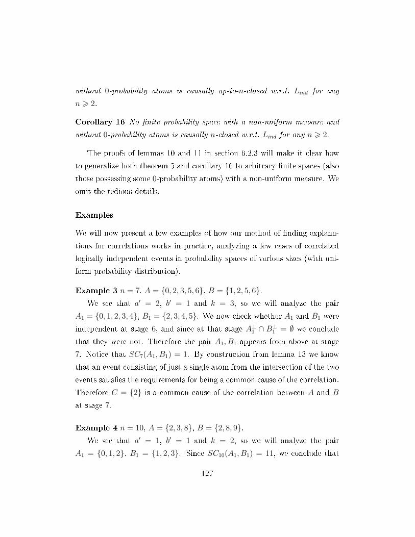
without 0-probability atoms is causally up-to-n-closed w.r.t. Lind for any
n > 2.
Corollary 16 No nite probability space with a non-uniform measure and
without 0-probability atoms is causally n-closed w.r.t. Lind for any n > 2.
The proofs of lemmas 10 and 11 in section 6.2.3 will make it clear how
to generalize both theorem 5 and corollary 16 to arbitrary nite spaces (also
those possessing some 0-probability atoms) with a non-uniform measure. We
omit the tedious details.
Examples
We will now present a few examples of how our method of nding explana-
tions for correlations works in practice, analyzing a few cases of correlated
logically independent events in probability spaces of various sizes (with uni-
form probability distribution).
Example 3 n = 7, A = 0, 2, 3, 5, 6, B = 1, 2, 5, 6.We see that a′ = 2, b′ = 1 and k = 3, so we will analyze the pair
A1 = 0, 1, 2, 3, 4, B1 = 2, 3, 4, 5. We now check whether A1 and B1 were
independent at stage 6, and since at that stage A⊥1 ∩ B⊥1 = ∅ we conclude
that they were not. Therefore the pair A1, B1 appears from above at stage
7. Notice that SC7(A1, B1) = 1. By construction from lemma 13 we know
that an event consisting of just a single atom from the intersection of the two
events satises the requirements for being a common cause of the correlation.
Therefore C = 2 is a common cause of the correlation between A and B
at stage 7.
Example 4 n = 10, A = 2, 3, 8, B = 2, 8, 9.We see that a′ = 1, b′ = 1 and k = 2, so we will analyze the pair
A1 = 0, 1, 2, B1 = 1, 2, 3. Since SC10(A1, B1) = 11, we conclude that
127

the lowest stage at which the pair is correlated is 5 (as remarked earlier, SC
changes by k from stage to stage). A1 and B1 are logically independent at
that stage, but not at stage 4, which means that the pair appears from above
at stage 5. We employ the same method as in the previous example to come
up with a 1-type common cause of the correlation at that stagelet it be the
event 1. Now the reasoning from case 2 of lemma 15 is used to `translate'
the explanation to stage 6, where it becomes the following 0-type SCCS:
1, 0, 2, 3, 4, 5. Case 3 of the same lemma allows us to arrive at an
SCCS for A1,B1 at stage 10: 1, 0, 2, 3, 4, 5, 6, 7, 8, 9. Its structure isas follows: one element contains a single atom from the intersection of the two
events, another the remainder of A1 ∪B1 as well as one atom not belonging
to any of the two events, while the third element of the SCCS contains the
rest of the atoms of the algebra at stage 10. We can therefore produce a
0-type SCCS for A and B at stage 10: 2, 0, 3, 8, 9, 1, 4, 5, 6, 7.
Example 5 n = 12, A = 2, 4, 6, 8, 9, 10, 11, B = 1, 3, 6, 10, 11.We see that a′ = 4, b′ = 2 and k = 3, so we will analyze the pair
A1 = 0, 1, 2, 3, 4, 5, 6, B1 = 4, 5, 6, 7, 8. We also see that A1 and B1
were logically independent at stage 11, but were not correlated at that stage.
Therefore the pair A1, B1 appears from below at stage 12. Notice that z = 3.
Therefore we see that z > b′ and a′ > k, which means we can use the method
from case 2 of lemma 14 to construct a 0-type common cause, whose comple-
ment consists of 1 atom from A1\B1 and 1 atom from (A1∪B1)⊥. Going back
to A and B, we see that the role of the complement of our common cause
can be fullled by C⊥ = 0, 2. Therefore C = 1, 3, 4, 5, 6, 7, 8, 9, 10, 11 isa 0-type common cause of the correlation between A and B at stage 12.8
8 Incidentally, if we wanted to nd a 1-type common cause for A and B at stage 12,
we could put C = 2, 11, in which case P (A | C) = 1. However, this is not always
possible and there are cases in which only 0-type common causes (or only 1-type common
128

6.2.3 Proofs of lemmas 9-11
Proof: [of lemma 9] If P is uniform, then 〈S, P 〉 has no 0-probability
atoms, which means that S = S+ and P = P+. Therefore P+ is uniform,
so (by theorem 3) 〈S+, P+〉 (and, consequently, 〈S, P 〉) is causally up-to-3-
closed w.r.t. L+ind. But in a space with no 0-probability atoms Lind = L+
ind,
therefore 〈S, P 〉 is also causally up-to-3-closed w.r.t. Lind.
The next two proofs will require jumping from 〈S+, P+〉 to 〈S, P 〉 andvice versa. We will now have to be careful about the distiction between
proper and improper SCC(S)s. Some preliminary remarks are in order.
Let A ∈ S. As before, we can think of A as a set of atoms of S. Let A+
be the set of non-zero probability atoms in A:
A+ := A \ a | a is an atom of S and P (a) = 0.
Notice that
P (A) =∑a∈A
P (a) =∑a∈A+
P (a) = P (A+) = P+(A+). (6.1)
Suppose A,B,C ∈ S. From (6.1) it follows that if A,B are correlated in
〈S, P 〉, A+, B+ are correlated in 〈S+, P+〉. Similarly, for any D ∈ S, P (D |C) = P+(D+ | C+). So, if C screens o the correlated events A,B in 〈S, P 〉,then C+ screens o the correlated events A+, B+ in 〈S+, P+〉. Also, if a
family C = Cii∈I satises the statistical relevance condition w.r.t. A,B
in 〈S, P 〉, then the family C+ = C+i i∈I satises the statistical relevance
condition w.r.t. A+, B+ in 〈S+, P+〉. If C = Cii∈0,...,n−1 is a proper
SCCS of size n for the correlation between events A,B in 〈S, P 〉, then all its
elements dier from both A and B by more than a measure zero event. It
causes) are possible. For a concrete example, take the pair 0, 1, 2, 3, 4, 4, 5, whichappears from below at stage 11 and has only 0-type common causes at that stage (we used
a computer program to verify this).
129

follows that in such a case C+ = C+i i∈0,...,n−1 is a proper SCCS of size n
for the correlation between events A+, B+ in 〈S+, P+〉.Proof: [of lemma 10] Since P+ is not uniform, by theorem 3 〈S+, P+〉
is not causally up-to-3-closed w.r.t. L+ind (and, consequently, Lind). Then
there exist logically independent, correlated events A+, B+ in S+ which do
not have a proper SCCS of size at most 3 in 〈S+, P+〉. The two events are
also logically independent and correlated in 〈S, P 〉; it is easy to show that
in 〈S, P 〉 the pair 〈A+, B+〉 also belongs both to L+ind and to Lind. We will
show that 〈S, P 〉 also contains no proper SCCS of size at most 3 for these
events. For suppose that for some m ∈ 2, 3, C = Cii∈N,i<m was a proper
SCCS of size m for the correlation between A+ and B+ in 〈S, P 〉. Then
C+ := C+i i∈N,i<m would be a proper SCCS of size m for the correlation
between A+ and B+ in 〈S+, P+〉, but by our assumption no such SCCSs
exist. We infer that the correlated events A+, B+ have no proper SCCS of
size up to 3 in 〈S, P 〉, so the space 〈S, P 〉 is not causally up-to-3-closed w.r.t.
either Lind or L+ind.
Proof: [of lemma 11] Since P+ is uniform, by theorem 3 〈S+, P+〉is causally up-to-3-closed w.r.t. L+
ind. We will rst show that also 〈S, P 〉 iscausally up-to-3-closed w.r.t. L+
ind. Notice that if A,B ∈ S are correlated
in 〈S, P 〉 and 〈A,B〉 ∈ L+ind, then A
+, B+ ∈ S+ are correlated in 〈S+, P+〉and 〈A+, B+〉 ∈ L+
ind. We know that in that case there exists in 〈S+, P+〉 aproper SCCS of size 2 or 3 for A+ and B+. If we add the 0-probability atoms
of S to one of the elements of the SCCS, we arrive at a proper SCCS of size
2 or 3 for A,B ∈ S.It remains to consider correlated events A,B ∈ S such that 〈A,B〉 ∈ Lind
but 〈A,B〉 /∈ L+ind. In such a case at least one of the probabilities from
denition 17 has to be equal to 0. It is easy to show that, since we know
the two events are correlated, it can only be the case that P (A ∩ B⊥) = 0
or P (B ∩ A⊥) = 0; equivalently, A+ ⊆ B+ or B+ ⊆ A+. It may happen
130

that A+ = B+. Let us rst deal with the case of a strict inclusion; suppose
without loss of generality that A+ ⊂ B+. If |B+ \ A+| > 1, take an event
C such that A+ ⊂ C ⊂ B+. Since both inclusions in the last formula are
strict, in such a case C is a proper statistical common cause for A and B.
Notice that since 〈A,B〉 ∈ Lind, from the fact that A+ ⊂ B+ it follows that
A 6= A+. Therefore, if |B+ \A+| = 1, put C = A+. Such a C is an improper
statistical common cause of A and B.
The last case is that in which A+ = B+. From the fact that A and B are
logically independent it follows that A \B+ 6= ∅ and B \ A+ 6= ∅. ThereforeA 6= A+ and B 6= B+. We can thus put C = A+ or C = B+ to arrive at an
improper statistical common cause of A and B.
When A+ ⊆ B+, it is also impossible to nd (even improper) SCCSs of
size 3 for A and B. For suppose C = Cii∈0,1,2 was an SCCS for A and
B. If for some j 6= l; j, l ∈ 0, 1, 2 it is true that Cj ∩ A+ = Cl ∩ A+ = ∅,then P (A|Cj) = 0 = P (A|Cl) and so C cannot be an SCCS of A and B
due to the statistical relevance condition being violated. Thus at least two
elements of C have to have a nonempty intersection with A+. Every such
element Cj screens o A from B. Since by our assumption A+ ⊆ B+, it
follows that P (AB|Cj) = P (A|Cj). Therefore the screening o condition
takes the form of P (A|Cj) = P (A|Cj)P (B|Cj); and so P (B|Cj) = 1. Since
we already established that C contains at least two elements which can play
the role of Cj in the last reasoning, it follows that in this case the statistical
relevance condition is violated too; all options exhausted, we conclude that
no SCCSs of size 3 exist for A and B when A+ ⊆ B+. The argument from this
paragraph can also be applied to show that if A+ ⊆ B+ and |B+ \ A+| 6 1,
no proper statistical common causes for the two events exist.
131

6.3 The proper / improper common cause
distinction and the relations of logical in-
dependence
A motivating intuition for the distinction between proper and improper com-
mon causes is that a correlation between two events should be explained by
a dierent event. The dierence between an event A and a cause C can
manifest itself on two levels: the algebraical (A and C being not identical as
elements of the event space) and the probabilistic (P (A∩C⊥) or P (C ∩A⊥)
being not equal to 0). As per denition 18, in the case of improper common
causes the dierence between them and at least one of the correlated events
(say, A) is only algebraical. For some this is intuitively enough to dismiss C
as an explanation for any correlation involving A.
One could, however, have intuitions to the contrary. First, events which
dier by a measure zero event can be conceptually distinct. Second, atoms
with probability 0 should perhaps be irrelevant when it comes to causal
features of the particular probability space, especially when the independence
relation considered is dened without any reference to probability. If the
space is causally up-to-n-closed w.r.t. Lind, adding 0-probability atoms should
not change its status. But consider what happens when we add a single 0-
probability atom to a space which is up-to-2-closed (common cause closed)
w.r.t. Lind by Proposition 3 from Gyenis & Rédei (2004): the space 〈S5, Pu〉,where S5 is the Boolean algebra with 5 atoms 0, 1, . . . , 4 and Pu is the
uniform measure on S5. Label the added 0-probability atom as the number
5. It is easy to check that the pair 〈3, 4, 4, 5〉 belongs to Lind, is correlatedand has no proper common cause. The only common cause for these events,
4, is improper. Therefore the space is not common cause closed w.r.t. Lind
in the sense of Gyenis & Rédei (2004) and our denition 19; this change
132
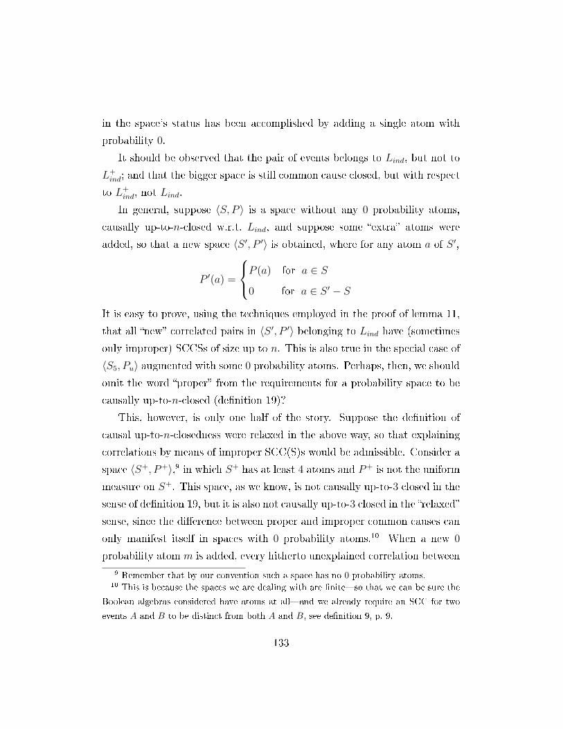
in the space's status has been accomplished by adding a single atom with
probability 0.
It should be observed that the pair of events belongs to Lind, but not to
L+ind; and that the bigger space is still common cause closed, but with respect
to L+ind, not Lind.
In general, suppose 〈S, P 〉 is a space without any 0 probability atoms,
causally up-to-n-closed w.r.t. Lind, and suppose some extra atoms were
added, so that a new space 〈S ′, P ′〉 is obtained, where for any atom a of S ′,
P ′(a) =
P (a) for a ∈ S
0 for a ∈ S ′ − S
It is easy to prove, using the techniques employed in the proof of lemma 11,
that all new correlated pairs in 〈S ′, P ′〉 belonging to Lind have (sometimes
only improper) SCCSs of size up to n. This is also true in the special case of
〈S5, Pu〉 augmented with some 0 probability atoms. Perhaps, then, we should
omit the word proper from the requirements for a probability space to be
causally up-to-n-closed (denition 19)?
This, however, is only one half of the story. Suppose the denition of
causal up-to-n-closedness were relaxed in the above way, so that explaining
correlations by means of improper SCC(S)s would be admissible. Consider a
space 〈S+, P+〉,9 in which S+ has at least 4 atoms and P+ is not the uniform
measure on S+. This space, as we know, is not causally up-to-3 closed in the
sense of denition 19, but it is also not causally up-to-3 closed in the relaxed
sense, since the dierence between proper and improper common causes can
only manifest itself in spaces with 0 probability atoms.10 When a new 0
probability atom m is added, every hitherto unexplained correlation between
9 Remember that by our convention such a space has no 0 probability atoms.10 This is because the spaces we are dealing with are niteso that we can be sure the
Boolean algebras considered have atoms at alland we already require an SCC for two
events A and B to be distinct from both A and B, see denition 9, p. 9.
133
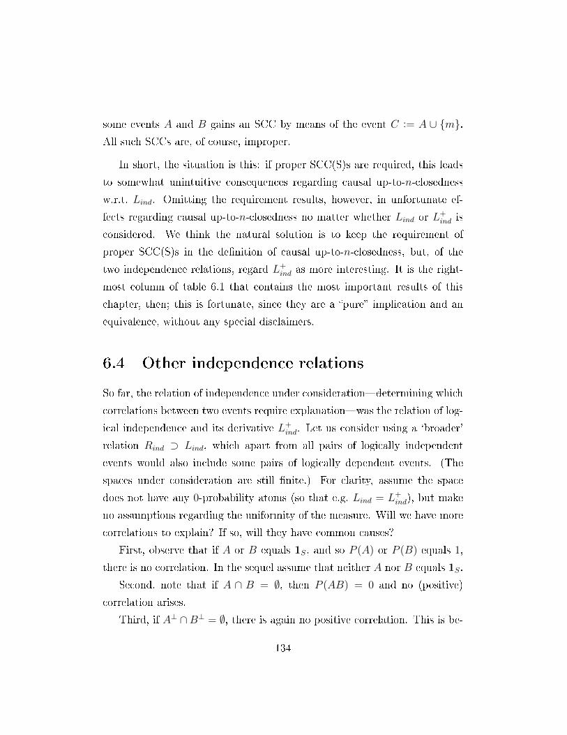
some events A and B gains an SCC by means of the event C := A ∪ m.All such SCCs are, of course, improper.
In short, the situation is this: if proper SCC(S)s are required, this leads
to somewhat unintuitive consequences regarding causal up-to-n-closedness
w.r.t. Lind. Omitting the requirement results, however, in unfortunate ef-
fects regarding causal up-to-n-closedness no matter whether Lind or L+ind is
considered. We think the natural solution is to keep the requirement of
proper SCC(S)s in the denition of causal up-to-n-closedness, but, of the
two independence relations, regard L+ind as more interesting. It is the right-
most column of table 6.1 that contains the most important results of this
chapter, then; this is fortunate, since they are a pure implication and an
equivalence, without any special disclaimers.
6.4 Other independence relations
So far, the relation of independence under considerationdetermining which
correlations between two events require explanationwas the relation of log-
ical independence and its derivative L+ind. Let us consider using a `broader'
relation Rind ⊃ Lind, which apart from all pairs of logically independent
events would also include some pairs of logically dependent events. (The
spaces under consideration are still nite.) For clarity, assume the space
does not have any 0-probability atoms (so that e.g. Lind = L+ind), but make
no assumptions regarding the uniformity of the measure. Will we have more
correlations to explain? If so, will they have common causes?
First, observe that if A or B equals 1S, and so P (A) or P (B) equals 1,
there is no correlation. In the sequel assume that neither A nor B equals 1S.
Second, note that if A ∩ B = ∅, then P (AB) = 0 and no (positive)
correlation arises.
Third, if A⊥ ∩B⊥ = ∅, there is again no positive correlation. This is be-
134

cause in such a case P (AB)+P (AB⊥)+P (A⊥B) = 1, and since P (A)P (B) =
P (AB)[P (AB) + P (AB⊥) + P (A⊥B)] + P (AB⊥)P (A⊥B) > P (AB), the
events are not correlated.
Consider the last possible conguration in which the events A,B are
logically dependent: namely, that one is a subset of the other. Suppose
A ⊆ B. Since by our assumption both P (A) and P (B) are strictly less than
1, the events will be correlated. It can easily be checked11 that when A ⊆ B
but B 6= 1S, any C which screens o the correlation and has a non-empty
intersection with A (and so P (A | C) 6= 0) has to be a subset of B (because
P (B | C) = 1). And since it cannot be that both C and C⊥ are subsets of
B, then if C is a common cause, it is necessary that C⊥ ∩ A = ∅. In the
other direction, it is evident that if A ⊆ C ⊆ B, both C and C⊥ screen o
the correlation and the statistical relevance condition is satised. The only
pitfall is that the denition of a common cause requires it be distinct from
both A and B, and so none exist when b′ = 1.
To summarize, the only correlated pairs of logically dependent events
A,B are these in which one of the events is included in the other. Assume
A ⊆ B. Then:
• if b′ = 1, there is no common cause of the correlation;
• otherwise the common causes of the correlation are precisely all the
events C such that A ⊂ C ⊂ B.
Lastly, notice that in a space 〈Sn, Pu〉 (Sn being the Boolean algebra
with n atoms and Pu being the uniform measure) we could proceed in the
opposite direction and restrict rather than broaden the relation Lind. If we
take the independence relation Rind to be the relation of logical independence
restricted to the pairs which appear from above or below at stage n, then
our probability space is common cause closed w.r.t. Rind.
11 See the last paragraph of the proof of lemma 11, p. 131.
135

6.5 A slight generalization
In this section we will show that the results of this chapter, which have only
concerned classical probability spaces so far, are also meaningful for nite
non-classical spaces. We go back to our former practice: by common cause
we will always mean proper common cause; similarly with common cause
system.
Denition 23 [Non-classical probability space] A lattice L is orthomo-
dular if ∀a,b∈L a 6 b⇒ b = a ∨ (a⊥ ∧ b).Two elements a and b of L are orthogonal i a 6 b⊥.
An additive state on an orthomodular lattice (OML) L is a map P from
L to [0, 1] such that P (1L) = 1 and for any A ⊆ L such that A consists of
mutually orthogonal elements, if∨A exists, then P (
∨A) =
∑a∈A P (a).12
A non-classical probability space is a pair 〈L, P 〉, where L is a non-
distributive OML and P is an additive state on L.13
A relation of compatibility needs to be introduced. Only compatible
events may be correlated; and a common cause needs to be compatible with
12 Of course, in the nite casesince a lattice always contains all suprema of doubletons
by virtue of being a latticeit would suce to say that for any two orthogonal elements
a and b, P (a ∨ b) = P (a) + P (b). However, innite lattices can be incomplete: they can
lack the suprema of certain subsets.13 A dierent direction could be taken in presenting the denitions of classical and non-
classical probability spaces: rst, a probability space could be dened as a measure on
an OML; then, classical and non-classical spaces could be distinguished on the basis of
whether the OML in question is distributive (in which case it is by denition a Boolean
algebra) or not. However, throughout the biggest part of this essay we have been in the
sphere of classical probability and so the term probability space was eectively short for
classical probability space. We do not want to change this more than halfway through
the work. However, for claricatory reasons, this will result in some denitions containing
the phrase classical or non-classical, perhaps redundant at rst sightsee e.g. denitions
25 and 26 below.
136
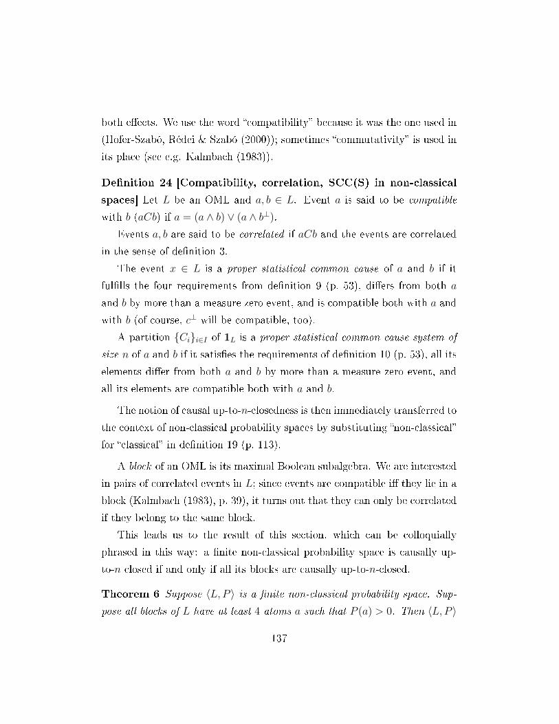
both eects. We use the word compatibility because it was the one used in
(Hofer-Szabó, Rédei & Szabó (2000)); sometimes commutativity is used in
its place (see e.g. Kalmbach (1983)).
Denition 24 [Compatibility, correlation, SCC(S) in non-classical
spaces] Let L be an OML and a, b ∈ L. Event a is said to be compatible
with b (aCb) if a = (a ∧ b) ∨ (a ∧ b⊥).
Events a, b are said to be correlated if aCb and the events are correlated
in the sense of denition 3.
The event x ∈ L is a proper statistical common cause of a and b if it
fullls the four requirements from denition 9 (p. 53), diers from both a
and b by more than a measure zero event, and is compatible both with a and
with b (of course, c⊥ will be compatible, too).
A partition Cii∈I of 1L is a proper statistical common cause system of
size n of a and b if it satises the requirements of denition 10 (p. 53), all its
elements dier from both a and b by more than a measure zero event, and
all its elements are compatible both with a and b.
The notion of causal up-to-n-closedness is then immediately transferred to
the context of non-classical probability spaces by substituting non-classical
for classical in denition 19 (p. 113).
A block of an OML is its maximal Boolean subalgebra. We are interested
in pairs of correlated events in L; since events are compatible i they lie in a
block (Kalmbach (1983), p. 39), it turns out that they can only be correlated
if they belong to the same block.
This leads us to the result of this section, which can be colloquially
phrased in this way: a nite non-classical probability space is causally up-
to-n closed if and only if all its blocks are causally up-to-n-closed.
Theorem 6 Suppose 〈L, P 〉 is a nite non-classical probability space. Sup-
pose all blocks of L have at least 4 atoms a such that P (a) > 0. Then 〈L, P 〉
137

is causally up-to-n-closed w.r.t Lind if and only if for any block B of L, the
classical probability space 〈B,P |B〉 is causally up-to-n-closed w.r.t. Lind.
Proof: Suppose 〈L, P 〉 is causally up-to-n-closed w.r.t. Lind. Let B be a
block of L; let a, b be correlated and logically independent events in 〈B,P |B〉.Then a, b are correlated and logically independent events in 〈L, P 〉, and so
have an SCCS of size up to n in 〈L, P 〉. But since all elements of the SCCS
have to be compatible with a and b, they also have to belong to B. And so
the pair has an SCCS of size up to-n in 〈B,P |B〉.For the other direction, suppose that for any block B of L, the space
〈B,P |B〉 is causally up-to-n-closed w.r.t. Lind. Let a, b be correlated and
logically independent events in 〈L, P 〉. Being correlated entails being com-
patible; and so a and b belong to a block B. Since the ordering on L is
induced by the orderings of the elements of B, a and b are also logically
independent in B. Therefore by our assumption they have an SCCS of size
up to n in 〈B,P |B〉. This SCCS is a partition of unity of L, and so satises
denition 24. Thus a and b have an SCCS of size up to n in 〈L, P 〉.
6.5.1 Examples
We will now present a few examples of causal closedness and up-to-3-closedness
of non-classical probability spaces. Figure 1 depicts two non-classical prob-
ability spaces causally closed w.r.t. L+ind. Notice that all blocks have exactly
5 atoms of non-zero probability and each such atom receives probability 15,
and so each block is causally closed w.r.t. L+ind. The left space is also causally
closed w.r.t. Lind.
The left OML in gure 2 has two blocks and the measure of the space is
uniform on both of them, therefore the space is causally up-to-3-closed w.r.t.
Lind. This however is not the case with the right one: its measure is not
uniform on the block with four atoms, and so there is a correlation among
138

Figure 6.1: Greechie diagrams of two OMLs which, if supplied with the state
which assigns number 15to all white atoms and 0 to both black atoms,
form non-classical probability spaces which are causally up-to-2-closed (or
simply causally closed, to use the term of Gyenis & Rédei (2004)) w.r.t.
L+ind.
some two logically independent events from that block which has neither a
common cause nor an SCCS of size 3. (One of these events will contain one
dotted atom and the single white atom of the block; the other will contain
two dotted atoms.) Therefore the space is not causally up-to-3-closed w.r.t.
Lind.
6.6 Application for constructing Bayesian net-
worksa negative opinion
One could entertain the thought that the algorithm outlined above, which
describes the construction of SCCs and SCCSs for pairs of logically inde-
pendent, correlated events in nite classical probability spaces with the uni-
form measure could be useful in the process of constructing a Bayesian net-
work; the prospect seems to be encouraging since the networks consist of
139

Figure 6.2: In these OMLs white atoms have probability 17and the dotted
ones 27. The space depicted on the left is causally up-to-3-closed, but the one
on the right is not.
a nite number of variables with each having a nite set of possible values
(Williamson (2005)). Suppose we have a xed population on which we are
doing our research, but we are not sure what variables should belong to the
causal structure, apart from some we are certain of. Suppose two correlated
variables, X and Y , belong to the group of which we are certain that it has
a rightful place in the structure, but no other variable we are similarly sure
of can be a common ancestor of X and Y in our projected DAG, since no set
of variables under consideration (dierent from X and Y ) makes X and Y
independent when conditioned upon. Could the algorithm presented above
allow us to construct an additional node for our Bayesian network, repre-
senting a variable we were not aware of when initially considering the causal
structure in question; which, when conditioned on, would render the corre-
lated variables independent? Unfortunately, the answer is no; it will bring
us back to the topic of common and common common screener systems.
The reason for the negative conclusion is the fact that a correlation be-
tween variables typically entails numerous correlations between events. The
argument above provides an explanation for any single correlation between
logically independent events, but there is no guarantee that a way exists of
somehow combining the events (= common causes), or three element par-
140

titions of the population (= SCCSs), in order to create a random variable,
which is what we need if we want to put a new node in our DAG.
A few simple abstract examples will clarify this. First, a fortunate case.
Consider an 8-element universe Ω = 0, 1, . . . , 7 and two correlated random
variables A and B, dened in this way:
A(x) =
1, x ∈ 0, 1;
2, x ∈ 2, 3;
3, x ∈ 4, 5, 6, 7;
B(x) =
1, x ∈ 0, 3;
2, x ∈ 1, 2;
3, x ∈ 4, 5, 6, 7.
There are some cases of correlated events (assume the uniform measure on Ω),
e.g. P (A = 1∧B = 2) > P (A = 1)P (B = 2) and P (A = 2∧B = 2) > P (A =
2)P (B = 2). If we run our procedure outlined in the preceding sections, we
arrive at the event C = 0, 1, 2, 3, which happens to be a common statistical
common cause for all correlations. Therefore we can dene it as a random
variable:
C(x) =
1, x ∈ 0, 1, 2, 3;
2, x ∈ 4, 5, 6, 7
which may be a candidate for a node in our DAG, since it satises the re-
quirement for a common ancestor of A and B, making them independent
when conditioned upon.14 In fact, being an SCC is overkill here; it is evi-
dent that being a common common screener system suces. Of course, as
noted in chapter 3 trivial systems of this kind always exist, but one could be
hopeful that our procedure may generate non-trivial systems for subsequent
consideration.
Unfortunately, in general this is not the case. Consider a smaller, 7-ele-
ment universe Ω = 0, 1, . . . , 6 and two correlated random variables A and
14 More precisely, the requirement is that the set of all common ancestors should make
the correlated variables independent when conditioned upon. By assumption, we do not
have other common ancestors of the events in question in our graph.
141
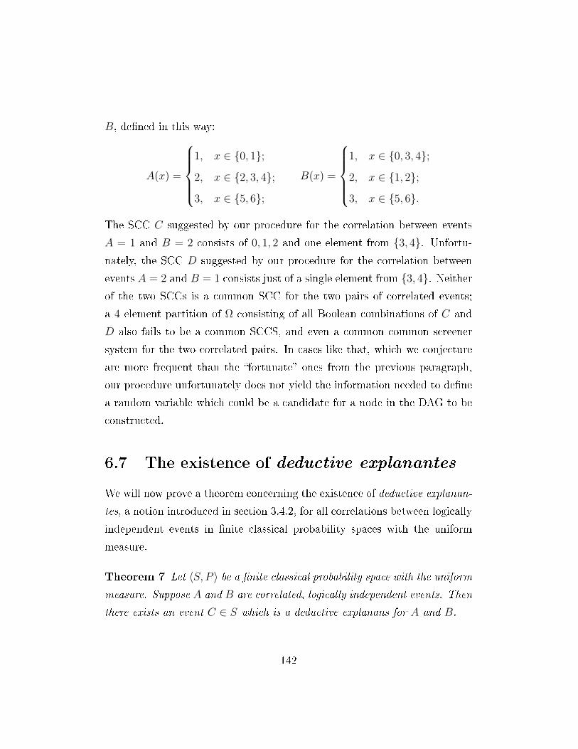
B, dened in this way:
A(x) =
1, x ∈ 0, 1;
2, x ∈ 2, 3, 4;
3, x ∈ 5, 6;
B(x) =
1, x ∈ 0, 3, 4;
2, x ∈ 1, 2;
3, x ∈ 5, 6.
The SCC C suggested by our procedure for the correlation between events
A = 1 and B = 2 consists of 0, 1, 2 and one element from 3, 4. Unfortu-
nately, the SCC D suggested by our procedure for the correlation between
events A = 2 and B = 1 consists just of a single element from 3, 4. Neitherof the two SCCs is a common SCC for the two pairs of correlated events;
a 4 element partition of Ω consisting of all Boolean combinations of C and
D also fails to be a common SCCS, and even a common common screener
system for the two correlated pairs. In cases like that, which we conjecture
are more frequent than the fortunate ones from the previous paragraph,
our procedure unfortunately does not yield the information needed to dene
a random variable which could be a candidate for a node in the DAG to be
constructed.
6.7 The existence of deductive explanantes
We will now prove a theorem concerning the existence of deductive explanan-
tes, a notion introduced in section 3.4.2, for all correlations between logically
independent events in nite classical probability spaces with the uniform
measure.
Theorem 7 Let 〈S, P 〉 be a nite classical probability space with the uniformmeasure. Suppose A and B are correlated, logically independent events. Then
there exists an event C ∈ S which is a deductive explanans for A and B.
142

Proof: Again, without loss of generality we can consider S as an n-atom
Boolean algebra of all subsets of the set 0, . . . , n−1; in other words, as the
probability space we would refer to as stage n in the preceding sections.
The deductive explanans for A and B will be the common cause C for them
at the (possibly lower) stage at which they appear, either from above or from
below.
Suppose that at stage m 6 n, where A and B appear, the method de-
scribed in the proofs of lemmas 13 and 14 ascribes them a statistical common
cause C. This C of course also screens o A in B at stage n. However, at
stage n C⊥ may be bigger then C⊥ at stage m: the dierence is n − m
atoms. C⊥ screens o A from B at stage m. The addition of even a single
atom to C⊥ has to break the condition, since the atom has non-zero prob-
ability (due to the measure being uniform) and belongs to neither A nor
B. It will make A and B correlated conditional on C⊥; at stage m + 1,
P (AB|C⊥) > P (A|C⊥)P (B|C⊥).
To see this, recall lemma 12: if two events are independent at some stage,
they are correlated at every later stage. Now consider a probability space
where the event space is the Boolean algebra with the set of atoms consisting
of the set of atoms of B restricted to C⊥ at stage m, and the measure is the
corresponding restriction of P . This algebra is isomorphic to the space at
stage k, where k is the cardinality of C⊥. Events A and B are independent
at stage k, but due to lemma 12 are correlated at stage k + 1. Thus, when
an additional atom is appended to C⊥, events A and B become correlated
conditional on C⊥. By the above argument, adding more atoms to C⊥ does
not change the fact that A and B are correlated conditional on it. And so,
at stage n it has to be the case that P (AB|C⊥) > P (A|C⊥)P (B|C⊥).
Since C is a common cause of A and B at stagem, at that stage P (A|C) >
P (A|C⊥) and P (B|C) > P (B|C⊥). When we move to higher stages, it
is evident P (A|C) and P (B|C) stay the same, while both P (A|C⊥) and
143

P (B|C⊥) decrease. Therefore STAT (A,C) and STAT (B,C) are true at
stage n, too.
Lastly, it is just a matter of consulting inequality 3.3 on page 70 to see that
C is a deductive explanans for A and B: the left-hand side of the inequality
is positive, while the right-hand side is negative.
So far, nothing has been established regarding the existenceor nonexi-
stenceof deductive explanantes for events in nite spaces with non-uniform
measures, or in innite spaces.
6.8 Conclusions and problems
The main result of this chapter is that in nite classical probability spaces
with the uniform probability measure (and so no atoms with probability 0)
all correlations between logically independent events have an explanation by
means of a common cause or a common cause system of size 3. A few remarks
are in order.
First, notice that the only SCCSs employed in our method described
in section 6.2.2 are 0-type SCCSs, and that they are required only when
`translating' the explanation from a smaller space to a bigger one. Sometimes
(if the common cause we found in the smaller space is 0-type; see example 5
above) such a translation can succeed without invoking the notion of SCCS
at all.
Second, #-type common causes, which some would view as `genuinely
indeterministic', are never required to explain a correlation that is, a corre-
lation can always be explained by means of a 0-type SCCS, a 0-type statis-
tical common cause, or a 1-type statistical common cause15. Therefore one
15 But #-type common causes do exist: e.g. in the space with 12 atoms and the uniform
measure the pair of events A, B, where A = 0, 1, 2, 3, 4, 5, 6, B = 4, 5, 6, 7, 8 (thesame we dealt with in example 5, p. 128) has, apart from both 0- and 1-type common
144

direction of the equivalence in theorem 4 can be strengthened:
Theorem 8 Let 〈S, P 〉 be a nite classical probability space. Let S+ be the
subalgebra of S containing all and only the non-zero probability atoms of S
and P+ be the restriction of P to S+. Suppose S+ has at least 4 atoms.
If P+ is the uniform probability measure on S+, then any pair of correlated
and logically independent events in 〈S, P 〉 has a 1-type statistical common
cause, a 0-type statistical common cause or a 0-type statistical common cause
system of size 3 in 〈S, P 〉.
6.9 Causal closedness of atomless spaces
Let us recall an important theorem from Gyenis & Rédei (2004) which we
will use in the next chapter. We move to the general context of possibly
innite probability spaces.
Denition 25 [Atomless probability space] A (classical or non-classical)
probability space 〈F , µ〉 is atomless if for any C ∈ F , if µ(C) > 0, then there
exists D ∈ F such that D ⊆ C and 0 < µ(D) < µ(C).
Of course, an atomless space may consist of a measure dened on an
atomic algebra (take the example of all Borel subsets of [0, 1] ⊆ R with the
Lebesgue measure).
We will rst focus on the classical case. It is obvious from the above
denition that in any classical atomless space, for any non-zero measure
event C there is an innite sequence of events with positive measure which
are its subsets. It could be contemplated, though, that some real numbers
less than µ(C) are not exhibited as probabilities of events being subsets of
causes, a #-type common cause of shape C = 1, 2, 4, 5, 7, 9, C⊥ = 0, 3, 6, 8, 10, 11;P (A | C) = 2
3 , P (B | C) =12 , P (A | C
⊥) = 12 , P (B | C
⊥) = 13 .
145

C. This is impossible! Gyenis & Rédei (2004) use a fact concerning classical
atomless spaces (see e.g. p. 46 of Fremlin (2001)), according to which, if for
some C µ(C) > 0, then for any real number r such that 0 < r < µ(C) there
exists a D ∈ F such that D ⊆ C and µ(D) = r. This allows the authors to
prove the following fact:
Fact 17 (Gyenis & Rédei (2004)) All atomless classical probability spa-
ces are causally closed.
Kitajima (2008) extended Gyenis' and Rédei's result to a special class
of non-classical spaces: these in which the OML on which the measure is
dened is atomless and complete (has suprema of all its subsets). Kitajima
proves that in such a case the non-classical probability space is atomless, too,
and that all such spaces contain SCCs for each pair of logically independent,
correlated events. We state Kitajima's result in the following form:
Fact 18 (Kitajima (2008)) If in a non-classical probability space 〈L, P 〉L is an atomless and complete OML, then 〈L, P 〉 is causally closed w.r.t. the
relation of logical independence.
146

Chapter 7
Causal completability
This chapter concerns the formulation of PCC we have dubbed PCC 4 (p.
19). The published results concerning causal completability (see e.g. Hofer-
Szabó et al. (1999)) are always formulated in the pair-style of thinking
about probability spaces: the one used in the previous chapter, according to
which a probability space is an algebra-measure pair with no mention of a
sample space. However, the main theorem of this chapter, theorem 10, due
to its very nature has to be phrased in a way which uses sample spaces. We
will therefore be switching from one way of writing to the other. In sections
7.1 and 7.2 we will write in the pair-style, while in section 7.3 we will use
the traditional, triadic notation.
The notion of an extension of a probability space was dened for proba-
bility spaces thought of as 3-tuples (denition 8, p. 19). We now repeat it in
the pair-style, omitting the sample space, which allows us to switch to the
more general formulation which is also applicable to non-classical spaces:
Denition 26 [Extension] A (classical or non-classical) probability space
〈S ′, µ′〉 is called an extension of the probability space 〈S, µ〉 i there exists
an orthomodular lattice embedding h of S into S ′ such that for any E ∈ S,µ(E) = µ′(E ′).
147

The idea of PCC 4 is that, even though there are some unexplained
correlations in a given space, an extension of it might exist which would
contain the required explanations. Such a case may represent a situation
in which, initially, not all important factors are taken into accountand a
more ne-grained probability space contains elements which do the job of
explaining the correlations.
7.1 Known results (the classical case)
In Hofer-Szabó, Rédei & Szabó (1999) the authors discuss causal completabil-
ity with regard to a family of correlated pairs of events. Their main result
regarding classical probability spaces follows, in a bit dierent formulation.
Denition 27 [Causal completability] Suppose 〈S, P 〉 is a probability
space and F is a family of pairs of correlated events which do not have
an SCC in 〈S, P 〉. The space 〈S, P 〉 is causally completable with regard to
the family F if there exists an extension 〈S ′, P ′〉 of 〈S, P 〉 by means of a
homomorphism h which contains an SCC for 〈h(A), h(B)〉 for every pair
〈A,B〉 ∈ F .
Fact 19 (Propos. 2 fromHofer-Szabó, Rédei & Szabó (1999)) Every
classical probability space is causally completable with regard to any nite
family of correlated events.
Hofer-Szabó et al. (1999) pose the problem whether classical probability
spaces are causally completable with regard to innite families of correlated
events. This we answer in the positive in section 7.3.
Of course, an extension of a given space which provides explanations
for some correlations may very well introduce new unexplained correlations.
The extension constructed by Hofer-Szabó et al. (1999) is not expected to
148
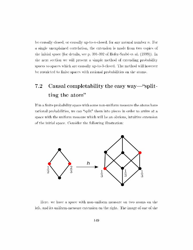
be causally closed, or causally up-to-n-closed, for any natural number n. For
a single unexplained correlation, the extension is made from two copies of
the initial space (for details, see p. 391-392 of Hofer-Szabó et al. (1999)). In
the next section we will present a simple method of extending probability
spaces to spaces which are causally up-to-3-closed. The method will however
be restricted to nite spaces with rational probabilities on the atoms.
7.2 Causal completability the easy waysplit-
ting the atom
If in a nite probability space with some non-uniform measure the atoms have
rational probabilities, we can split them into pieces in order to arrive at a
space with the uniform measure which will be an obvious, intuitive extension
of the initial space. Consider the following illustration:
Here, we have a space with non-uniform measure on two atoms on the
left, and its uniform-measure extension on the right. The image of one of the
149
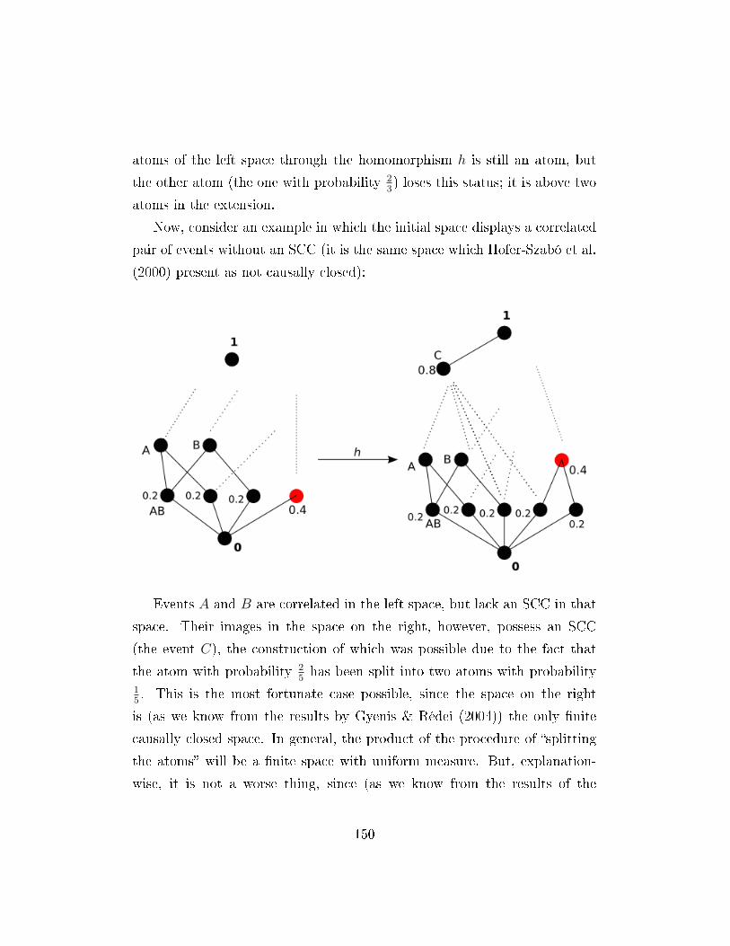
atoms of the left space through the homomorphism h is still an atom, but
the other atom (the one with probability 23) loses this status; it is above two
atoms in the extension.
Now, consider an example in which the initial space displays a correlated
pair of events without an SCC (it is the same space which Hofer-Szabó et al.
(2000) present as not causally closed):
Events A and B are correlated in the left space, but lack an SCC in that
space. Their images in the space on the right, however, possess an SCC
(the event C), the construction of which was possible due to the fact that
the atom with probability 25has been split into two atoms with probability
15. This is the most fortunate case possible, since the space on the right
is (as we know from the results by Gyenis & Rédei (2004)) the only nite
causally closed space. In general, the product of the procedure of splitting
the atoms will be a nite space with uniform measure. But, explanation-
wise, it is not a worse thing, since (as we know from the results of the
150

preceding chapter), all such spaces are causally up-to-3-closed (w.r.t. the
relation of logical independence).
Let us put together the above considerations in form of a theorem.
Theorem 9 Any nite probability space 〈S, P 〉 with rational probabilities on
the atoms of S has an extension which is causally up-to-3-closed w.r.t. the
relation of logical independence.
A sketch of the proof. The probabilities of the atoms a0, . . . , am of Sconstitute a nite list 〈p0, . . . , pm〉 of fractions. Calculate the lowest common
denominator D of these fractions. Let S ′ be the Boolean algebra with D
atoms b1, . . . , bD and let P ′ be the uniform measure on S ′. Transform all
the fractions 〈p0, . . . , pm〉 so that their denominator is D. Let 〈n0, . . . , nm〉be the list of numerators of the corresponding fractions from 〈p0, . . . , pm〉. Ofcourse,
∑mi=0 ni = D. Let h : S → S ′ be a homomorphism which assigns any
atom ai of S the supremum of ni atoms of S ′ in the following way:
h(a0) = b1, . . . , bn0;
h(a1) = bn0+1, bn0+n1;
· · ·
It is evident that 〈S ′, P ′〉 is an extension of 〈S, P 〉 by means of the homo-
morphism h. And by theorem 4 (p. 115), this extension is causally up-to-3
closed w.r.t. the relation of logical independence.
7.3 Causal completability of classical probabi-
lity spacesthe general case
A way of solving the general problem of causal completability with regard to
any family of correlated events would be to show that any space possesses
151
a causally closed extension. A result of Gyenis & Rédei (2004), reproduced
above as fact 17, states that all atomless spaces are causally closed. We
simply need to nd a way of extending an arbitrary space to an atomless
space. This is done in the proof of theorem 10. Let us state the initial
problem formally; it was posed in Hofer-Szabó et al. (1999) and Hofer-Szabó
et al. (2000):
Problem 2 (Causal completability of classical probability spaces)
Let 〈S, µ〉 be a probability space and W ⊆ S2 be the (possibly innite) family
of all pairs of correlated logically independent events for which no common
cause in 〈S, µ〉 exists. Is there an extension 〈S ′, µ′〉 (given by the embedding
h) of 〈S, µ〉 such that for any 〈D,E〉 ∈ W, there exists in 〈S ′, µ′〉 a common
cause for the pair 〈h(D), h(E)〉?
In view of fact 17, we can answer this problem by showing that any
classical probability space is extendable to an atomless space. We will use
the following lemma:
Lemma 20 Let 〈S,F , p〉 be a probability space and let 〈[0, 1],B, L〉 be the
space of all Borel subsets of the [0, 1] segment, L being the Lebesgue measure.
Then the product space 〈S × [0, 1],Σ, µ〉 of the two above spaces is atomless.
The proof uses the technique from chapter 211M of Fremlin (2001). For
the details on the construction of Σ, the event σ-algebra of the product space,
see e.g. chapter IV.6 of Feller (1968), vol. 2.
Proof: Let E ∈ Σ, µ(E) > 0. Let f be a function from [0, 12] to [0, 1]
given by the formula f(a) = µ(E ∩ (1F × [1
2− a, 1
2+ a])
). Observe that if
a, b ∈ [0, 12] and a 6 b, then f(a) 6 f(b) 6 f(a) + µ(1F × [1
2− b, 1
2+ b]) −
µ(1F×[12−a, 1
2+a]) = f(a)+p(1F)·L([1
2−b, 1
2+b])−p(1F)·L([1
2−a, 1
2+a]) =
f(a)+2b−2a. Therefore, f is continuous (as b approaches a, f(b) approaches
f(a)).
152

Notice that f(0) = 0 and limn→ 12f(n) = µ(E) > 0. Since we know that
f is continuous, we can apply the intermediate value theorem and conclude
that for some a ∈ (0, 12), 0 < f(a) < µ(E). That is,
0 < µ
(E ∩
(1F × [
1
2− a, 1
2+ a]
))< µ(E).
The event E ∩ (1F × [12− a, 1
2+ a]) is a subset of E and has a strictly lower
measure. Since E was arbitrary, 〈S × [0, 1],Σ, µ〉 is atomless.
The following theorem gives a positive answer to problem 2.
Theorem 10 Every probability space can be extended to a probability space
which is causally closed.
Proof: Let 〈S,F , p〉 be a probability space. From lemma 20 we know
that 〈S × [0, 1],Σ, µ〉, which is the product of 〈S,F , p〉 with the space of all
Borel subsets of the [0, 1] segment with the Lebesgue measure, is atomless.
Let h : F → Σ be dened as h(D) = D × [0, 1]. It is immediate that h
is a Boolean algebra embedding of F into Σ, and so 〈S × [0, 1],Σ, µ〉 is anextension of 〈S,F , p〉. Moreover, from fact 17 we infer that it is a causally
closed extension of 〈S,F , p〉.
Therefore, PCC 4 is a true principle. Of course, it is not very practical. To
make a brief foray into decidedly non-formal matters, perhaps a god or some
other vastly knowledgeable entity could envisage an uncountable probability
space which takes into account every possible factor and contains SCCs for
all possible correlations of logically independent events. The role of PCC 4
would be that of reassurance of us puny humans.
153
7.4 Causal completability of non-classical pro-
bability spacessome known results and
prospects
Another result from Hofer-Szabó et al. (1999) says that every nonclassical
space with an additive state µ has an extension containing SCCs for every
pair correlated in µ:
Fact 21 (Proposition 3 from Hofer-Szabó et al. (1999)) Let 〈S, µ〉 bea non-classical probability space. Let F be the family of all pairs of events
correlated in µ. Then 〈S, µ〉 is causally completable w.r.t. the family F .
However, one could ask the question similar to the one answered in
the previous section: is any non-classical probability space extendable to
a causally closed non-classical probability space? So far, the answer to this
question is not known.
One way of approaching the problem would be to try to use Kitajima's
result presented above as fact 18. The task would then boil down to the
following: given a non-classical space 〈L, P 〉, nd its extension 〈L′, P ′〉 withan atomless L′. The extension would have to be an atomless non-classical
probability space and would be, by fact 18, causally closed w.r.t. Lind.
Unfortunately, it seems we should not count on using a method similar
to the one outlined in the previous section. The strategy was this: take
a Boolean algebra and construct a product of it and an (atomic) Boolean
algebra being the event space of an atomless probability space. The crucial
point is that there is a subalgebra in the product which is isomorphic to
the original algebra. Thus we can nd a homomorphism due to which the
product can serve as the event space for an extension of the original space.
Algebraically speaking, the above fact can be phrased as for any Boolean
algebras A and B, A is a retract of A×B (see p. 90 of Koppelberg (1989)).
154

However, once we switch to non-distributive lattices, we can no longer count
on this. If A is a non-distributive OML and B is a Boolean algebra, it may
happen that the product A×B does not contain a subalgebra isomorphic to
A. Thus such a product in general does not seem to be a good candidate for
the OML on which an additive state could be dened so that the resulting
non-classical probability space would be an extension of the initial space.
To see this, take the product of the so called Chinese lantern (on the
left) and the two-element Boolean algebra:
which is the following orthomodular lattice:
155

The orthocomplement function has not been displayed on the pictures,
but it can be easily checked that the above lattice does not have a subalgebra
isomorphic to the Chinese lantern for any proper ascription of orthocomple-
ments.1
Therefore, when trying to construct for a given OML L an OML L′ which
would contain a subalgebra isomorphic to L, taking a product of L and some
other OML may be a bad move.2 This is even before we take into account
the fact that we would like to require that L′ be atomless and complete. In
fact, the general issue whether every OML can be embedded into a complete
OML is a long-standing open problem (see e.g. chapter 8 in Bruns & Harding
(2000)).
1 The point could perhaps be made clearer if we restricted our attention just to the two
lattice operations ∨ and ∧: the last OML represented not only does not have a subalgebra
isomorphic to the Chinese lantern taken as an algebra with three operations, but (which
is immediately seen) does not even have a sublattice isomorphic to the Chinese lantern
taken as a lattice.2 Of course, our example presented a quite special case, since the other OML in it
was Boolean.
156

Chapter 8
Statistical ε-common causes
We have seen in section 3.4.1 that weakening the requirement of perfect
screening o to even a minuscule degree results in the concept of SCC losing
the deductive explanatory feature. But let us put an epistemic twist on the
argument. Suppose we are investigating a population in which seemingly
causally unrelated attributes A and B are correlated; our goal is to nd
a common cause for the two attributes. Of course, our carefully chosen
samplejust like the populationis nite; suppose we discover an attribute
C such that the frequencies of A, B and C in the sample are very close to
screening o:∣∣∣fr(ABC)
fr(C)− fr(AC)
fr(C)fr(BC)fr(C)
∣∣∣ < ε for some small ε (e.g. 0.01); we will
say that the screening o condition is violated to the degree of ε. We would
of course be inclined to infer that we found a screener o for A and B, an
event which stands in the appropriate probabilistic relation to them, even if
this relation is not ideally represented by the sample frequencies (and perhaps
the whole population frequencies). But the experimental results are also fully
consistent with a dierent situation, in which C is not a perfect screener for
A and Bfor example, the screening o condition may be violated to the
degree of ε, with the sample frequencies giving a good illustration of the
real probabilistic picture. We, however, would be fully oblivious of this,
157

and would consider C a screener for the correlation between A and B.
Suppose, for example, that we are examining a population of 20000 units,
investigating a correlation between two attributes A and B such that fr(A) =
4997, fr(B) = 5001 and fr(AB) = 2498. Suppose further that we nd an
attribute C such that fr(C) = 10004, and that it turns out that A and B are
both necessary conditions for C. In such a case,∣∣∣fr(ABC)
fr(C)− fr(AC)
fr(C)fr(BC)fr(C)
∣∣∣ =
0.00000005. Does C screen o A from B? It may very well happen that it
does not, that in fact it does violate the screening o condition to a minuscule
degree, and thus does not possess the deductive explanatory featureand we
do not have any way to nd this out! Without any further information, we
are tempted to judge that the attribute C is a perfect screener o for A
and B, and in this case is their statistical common cause.
This shows that, even though we already know that nite spaces with
non-uniform distributions are not causally up-to-n closed for any n ∈ N, itwill be worthwhile to study such spaces with a dierent idea in mind: that
of nding for a given correlation an approximate statistical common cause
(system), which could be experimentally indistinguishable from a perfect
SCC(S).
Denition 28 [Statistical ε-common cause, statistical ε-common cau-
se system] Let 〈Ω,F , P 〉 be a probability space. Let A,B ∈ F and ε be a
positive real number lower than 0.25. If there exists C ∈ F dierent from
both A and B such that∣∣∣P (AB | C) = P (A | C)P (B | C)∣∣∣ 6 ε;∣∣∣P (AB | C⊥) = P (A | C⊥)P (B | C⊥)∣∣∣ 6 ε;
P (A | C) > P (A | C⊥);
P (B | C) > P (B | C⊥),
then C is called a statistical ε-common cause (ε-SCC) of A and B.
158

A partition of unity of F is said to be a statistical ε-common cause system
(ε-SCCS) for A and B if it satises the statistical relevance condition w.r.t. A
and B, all its members are dierent from both A and B, and all its members
C satisfy the condition∣∣∣P (AB | C) = P (A | C)P (B | C)∣∣∣ 6 ε.
The cardinality of the partition is called the size of the statistical ε-common
cause system.
A point similar to the experimental non-detectability of perfect screening
o could be made regarding the conditions of statistical relevance. Perhaps
an event C is statistically relevant for A and B when probabilities are con-
cerned, but the relevance is so weak that it is typically not displayed in
the observed frequencies? It is evident how the above denition could be
amended to take this into account; howeversince the conditions of sta-
tistical relevance are in general less frequently used than the screening o
conditions, e.g. in the Bayesian networks approachwe will only note that,
paraphrasing a sentence from chapter 3, in search for statistical ε-common
causes, (weakened) screening o is not enough. The statistical relevance
conditions have to be explicitly checked. Tests conducted using the statis-
tical software R show, however, that this additional requirement does not
add to the diculty of nding ε-SCC(S)s in practice; weakened screening o
fails to be enough only very rarely.
In general, data gathered in the conducted tests show that the task of
nding ε-SCCSs for correlated events is surprisingly easy, even for a very
small ε. We begin with a systematic study of searching for SCCs only (i.e.
not for SCCSs of size bigger than 2) in probability spaces with binomial
distribution. We then present three cases of searches for 2- and 3-element
SCCSs in spaces with distributions skewed in dierent ways.
159
The testing procedure was similar in all cases. A probability distribution
in a nite probability space, the event space of which has n atoms, can be
represented as a vector consisting of n real numbers from the [0, 1] segment
which together give 1 as their sum. An event in an n-atomic event space,
thought of as a set of atoms, can be represented as an n-element 0-1 sequence:
a 1 in position k means that the atom number k belongs to the event, a 0
means that it does not. To choose an event at random means, then, to
randomly choose a 0-1 sequence; the uniform distribution has been assumed
here (in contrast to the distributions of the spaces under consideration) so
that the process can be thought of as consisting of n tosses of a fair coin.
For any space, a certain number of randomly determined pairs of logically
independent events was tested. For any pair a search for an ε-SCC was
conducted. Since it would in general be not reasonable to set to check all
events in the given space (an n-atomic space has 2n events), a maximum of
n2 randomly chosen events were checked for each pair; in the case of binomial
distribution, presented in the next section, the even more stringent restriction
to (n − 1)2 was used. The check consisted of straightforward examination
whether the conditions from denition 28 are true in the given case. If yes,
next pair of correlated events was considered. All output was being logged.
The program returned the success ratio: the number of pairs for which an
ε-SCCS was found divided by the number of checked pairs.
8.1 Binomial distributions
A binomial distribution represents the odds of arriving at a given number
of successes in m trials with the chance of success s. The probability space
for m trials has n = m + 1 atoms (since it might happen that there are no
successes at all). Let a0 . . . am be all the atoms in the event space. The
chance for getting exactly k successes in m trials with the chance of success
160
s is given by the following formula:
P (ak) =
(m
k
)sk(1− s)m−k.
Since any event can be thought of as a set of atoms, calculating its probability
means simply summing the above expression for various values of k.
Nine probabilities of success were considered: from 0.9 to 0.1 with 0.1
decrement. Five degrees of approximation were used: from 0.05 to 0.01
with 0.01 decrement. We will present the results for the numbers of trials
ranging from 11 to 50; for example, the space for 11 trials has 12 atoms, but
in that particular case for each correlated pair 121 candidates for an ε-SCC
are checked. In a space for m trials, 4 · m2 pairs of logically independent,
correlated events were considered. The above parameters give us 1800 spaces;
however, the table depicting the results will be quite small. This is because,
with the success ratio rounded in the standard way, it turns out that even
for ε = 0.01, for the overwhelming majority of pairs of logically correlated
events it is possible to nd an SCCS just by checking a randomly chosen very
small portion of the whole event space.
Table 8.1 would be even simpler if we started with spaces with 13 atoms;
notice also that it is plausible that some of the lines, e.g. the one with the
strange behaviour of the space for s = 0.7 and 29 trials with ε = 0.01, can
be expected to disappear on repeated experiments. The picture is clear: in
spaces with the binomial distribution it is very easy to nd ε-SCCs empirically
indistinguishable from perfect SCCs.
8.2 A few contrastive examples
What about other non-uniform distributions? Our conjecture is that the
situation is similar and, while it might in general be impossible to nd (for
a given correlated pair) an event which would satisfy the requirements for
161

s ε # of trials Success ratio
0.1 - 0.9 0.03 - 0.05 11 - 50 1
0.3 - 0.7 0.02 11 0.9
0.3, 0.6, 0.7 0.02 12 - 50 1
0.5 0.02 12 - 14 0.9
0.5 0.02 15 - 50 1
0.4 0.02 13 0.9
0.4 0.02 12, 14 - 50 1
0.1, 0.2, 0.8, 0.9 0.01 11 - 50 1
0.3 - 0.6 0.01 13 - 50 0.9
0.7 0.01 13 - 28, 30 - 50 0.9
0.7 0.01 29 1
0.3, 0.6, 0.7 0.01 12 0.9
0.4, 0.5 0.01 12 0.8
0.3, 0.5 - 0.7 0.01 11 0.9
0.4 0.01 11 0.8
Table 8.1: Success ratios for nding ε-SCCs for correlated pairs of logically
independent events in spaces with the binomial distribution.
an SCC, it is relatively easy to nd an ε-SCC (or an ε-SCCS of size 3) for a
small value of ε. We have no general theorem; however, many dierent spaces
with variously skewed distributions have been checked and the conjecture,
informal as it may be, still stands. We will now present a few examples. In all
of the spaces considered 100 pairs of logically independent correlated events
were checked and the same values of ε were considered as above. However,
the search for explanation consisted of two phases. Suppose the space had n
atoms. First n2 candidates for ε-SCCs were considered. If no SCC was found,
then additional n2 candidates for ε-SCCSs of size 3 were investigated (each
162

candidate being represented by a randomly chosen n-element sequence of 0s,
1s and 2s). Usually, if for a given pair no ε-SCC was found, then no ε-SCCS
of size 3 was found, eitherbut there were exceptions. The numerator of the
success ratio consisted of pairs for which either an SCC or an SCCS of size
3 was found.
Example 6 The space consisted of 11 atoms, one with probability 0.9, the
remaining all with probability 0.01. The success ratio was 1 regardless of the
ε used.
Example 7 The space consisted of 22 atoms, two with probability 0.4, the re-
maining all with probability 0.01. The success ratio was 1 for ε ∈ 0.04, 0.05,0.99 for ε = 0.03, 0.97 for ε = 0.02, and 0.8 for ε = 0.01.
Example 8 The space consisted of 15 atoms, ve with probability 0.10,
and the remaining all with probability 0.05. The success ratio was 0.97 for
ε = 0.05, 0.96 for ε = 0.03, 0.95 for ε = 0.03, 0.89 for ε = 0.02, and 0.74 for
ε = 0.01.
Many other distributions have been tested; in all of them the success ratio
for ε = 0.01 was 0.74 or more. For a bit greater values of ε, the success ratio
is in general very close to 1. Remember that only a portion of the events
(or partitions, in case of SCCSs) in the given space served as candidates for
explanations during the tests! The high success ratio means that in general,
in an n-atomic space, searching through just n2 events (out of all 2n events)
and, if this fails, n2 3-element partitions of the unity of the space suces for
nding an ε-SCC or ε-SCCS for small values of ε.
While of course only a general mathematical argument could be ulti-
mately persuasive, the lesson should be clear, we think: even though nite
probability spaces with non-uniform measures are in general not causally up-
to-n closed for any natural n > 2, a vast majority of the correlated pairs of
163

logically correlated events can be expected to possess an ε-SCC or ε-SCCS
of size 3, which is experimentally indistinguishable from its perfect coun-
terpart.
164

Chapter 9
Conclusion
The main results of this study are included in chapters 6 and 7. Among them
are positive determinations concerning the prospects of explaining correla-
tions via statistical common cause systems. Perhaps of the biggest intuitive
force is theorem 10: every probability space can be extended to a probability
space which is causally closed. If we do not see a statistical common cause
for two correlated events, it is only because we have directed our attention
to the wrong probability space; there is an extension of it which leaves no
correlations unexplained. However, as foreshadowed in the introduction to
this essay, this can be interpreted in two ways. On the one hand, it is al-
ways nice to have a general positive theorem about the applicability of some
interesting notion. On the other hand, in this case the applicability may be
strictly mathematical. It is by no means evident that the statistical common
causes present in the extended spaces will have much to do with what we
would naturally accept as causes.
Consider again the example of particle decay from section 2.4.1. The
momentum of one part of the particle is determined in accordance with the
principle of conservation of total momentum by the momentum of the other
particle. Suppose the experimental setup is described by a probability space
165

S. The state of the particle before the decay event is, in this space, not a
screener o for the values of momentum after the split. Consider then the
causally closed space S ′, which is an extension of S, and which has to exist
by theorem 10. In this space the momenta of the two parts of the decayed
particle possess a statistical common cause which screens o one from the
other. But do we really expect such a screener to have anything to do with
the true causal picture? Are we not fully satised with the explanation
consisting of the principle of conservation of total momentum coupled with
the information on the genesis of the two particle parts?
Due to the generality of theorem 10 it is true that the big space used
in the eponymous approach to the Bell inequalities can also be extended to
a causally closed spacein which all correlations have common causes. This
may be surprising for those who think that this should lead to the empirically
falsied inequalities. This is, however, not the case, sinceas already noted
in the big space approach the EPR-type correlations are in fact conditional
correlations and so do not fall under the scope of theorem 10. And if we move
to the many spaces approach, then each of the small spaces will have
their own causally closed extension. However, it is by no means evident that
parameter independence, outcome independence and non-conspiracy should
hold for the extended spaces.
In conclusion, we should better be skeptical towards a general application
of explaining correlations by means of purely probabilistic dened notions.
Those employed in this essay, from Reichenbach's common cause as the mid-
dle element of a conjunctive fork, through statistical common cause systems,
to deductive explanantes, share (apart from screening o) the deductive ex-
planatory feature described in section 3.1. This is a pleasing fact which
strengthens the case for such notions playing a role in explanation, but it is
clearly not enough, e.g. since the correlation itselfas well as many other
more or less trivially equivalent (sets of) conditionsalso has that particular
166

feature. There is more to causal explanation than pure statistics. However,
mathematical methods like the algorithm of constructing SCCs and SCCSs
used in the proof of theorem 4 may provide candidates for explanationsfor
example, they may suggest searching for traits possessed by certain subsets
of the examined populationwhich can subsequently be studied by applying
other methods: using the previous knowledge of mechanisms operating in
the given context.
167

Bibliography
Adams, E. W. (1998). A Primer of Probability Logic. CSLI Publications
(Univ. of Chicago Press).
Arntzenius, F. (1992). The Common Cause Principle. PSA: Proceedings of
the Biennial Meeting of the Philosophy of Science Association, Vol. 1992,
Volume Two: Symposia and Invited Papers.
Arntzenius, F. (2005). Reichenbach's Common Cause Principle. In E. Zalta
(Ed.), The Stanford Encyclopedia of Philosophy (Winter 2008 Edition).
URL = <http://plato.stanford.edu/archives/win2008/entries/physics-
Rpcc/>.
Aspect, A., Dalibard, J., & Gérard, R. (1982). Experimental test of Bell's
Inequalities using time-varying analyzers. Physical Review Letters, 49,
18041807.
Bell, J. S. (1964). On the EinsteinPodolskyRosen Paradox. Physics, 1,
195200.
Belnap, N. & Szabó, L. E. (1996). Branching Space-Time Analysis of the
GHZ Theorem. Foundations of Physics, 26 (8), 9891002.
Berkovitz, J. (2000). The Many Principles of the Common Cause. Reports
on Philosophy, 20.
168
Berkovitz, J. (2008). Action at a Distance in QuantumMechanics. In E. Zalta
(Ed.), The Stanford Encyclopedia of Philosophy (Winter 2008 Edition).
URL = <http://plato.stanford.edu/archives/win2008/entries/qm-action-
distance/>.
Billingsley, P. (1995). Probability and Measure (3rd ed.). John Wiley & Sons,
Inc.
Blalock, H. (1979). Social Statistics (2nd ed.). McGraw-Hill.
Bruns, G. & Harding, J. (2000). Algebraic Aspects of Othomodular Lattices.
In B. Coecke, D. Moore, & A. Wilce (Eds.), Current research in operational
quantum logic: algebras, categories, languages (pp. 3765). Springer.
Buttereld, J. (1989). A Space-Time Approach to the Bell Inequality. In J. T.
Cushing & E. McMullin (Eds.), Philosophical Consequences of Quantum
Theory. Reections on Bell's Theorem. University of Notre Dame Press,
Indiana.
Buttereld, J. (2007). Stochastic Einstein Locality Revisited. The British
Journal for the Philosophy of Science, 58 (4), 805867.
Cartwright, N. (1988). How to tell a common cause: generalizations of the
conjunctive fork criterion. In J. H. Fetzer (Ed.), Probability and Causality
(pp. 181188). D. Reidel Publishing Company.
Cartwright, N. (1989). Nature's Capacities and Their Measurement. Oxford
University Press.
Cartwright, N. (1999). The Dappled World. A Study of the Boundaries of
Science. Cambridge University Press.
Clauser, J. F. & Horne, M. A. (1974). Experimental consequences of objective
local theories. Physical Review D, 10 (2), 526535.
169

Eberhardt, F. (2009). Reliability via synthetic a priori: Reichenbach's doc-
toral thesis on probability. Synthese, DOI 10.1007/s1122900995878.
Feller, W. (1968). An Introduction to Probability Theory and its Applications.
John Wiley & Sons, Inc.
Fine, A. (1982a). Hidden Variables, Joint Probability, and the Bell Inequal-
ities. Physical Review Letters, 48 (5), 291295.
Fine, A. (1982b). Some local models for correlation experiments. Synthese,
50, 279294.
Forster, M. R. (1988). Sober's Principle of Common Cause and the Problem
of Comparing Incomplete Hypotheses. Philosophy of Science, 55 (4), 538
559.
Fremlin, D. (2001). Measure Theory, volume 2. Torres Fremlin.
Glymour, C. (2010). What Is Right with 'Bayes Net Methods' and What Is
Wrong with 'Hunting Causes and Using Them'? The British Journal for
the Philosophy of Science, 61, 161211.
Graÿho, G., Portmann, S., & Wüthrich, A. (2005). Minimal Assumption
Derivation of a Bell-type Inequality. The British Journal for the Philosophy
of Science, 56, 663680.
Gyenis, B. & Rédei, M. (2004). When Can Statistical Theories be Causally
Closed? Foundations of Physics, 34 (9), 12841303.
Gyenis, B. & Rédei, M. (2010). Causal completeness in general probability
theories. In M. Suárez (Ed.), Probabilities, Causes, and Propensities in
Physics. Synthese Library, Springer.
170
Haig, B. D. (2003). What Is a Spurious Correlation? Understanding Statis-
tics, 2 (2), 125132.
Higashi, K. (2008). The Limits of Common Cause Approach to EPR Corre-
lation. Foundations of Physics, 38, 591609.
Hitchcock, C. (2010). Probabilistic Causation. In E. Zalta (Ed.),
The Stanford Encyclopedia of Philosophy (Summer 2010 Edition).
URL = <http://plato.stanford.edu/archives/sum2010/entries/causation-
probabilistic/>.
Hofer-Szabó, G. (2008). Separate- versus common-common-cause-type
derivations of the Bell inequalities. Synthese, 163, 199215.
Hofer-Szabó, G. (2010). Bell(δ) inequalities derived from sepa-
rate common causal explanation of almost perfect EPR anticorrela-
tions. Foundations of Physics, preprint archived at http://philsci
archive.pitt.edu/archive/00005371/.
Hofer-Szabó, G. & Rédei, M. (2004). Reichenbachian Common Cause Sys-
tems. International Journal of Theoretical Physics, 43 (7/8), 18191826.
Hofer-Szabó, G. & Rédei, M. (2006). Reichenbachian Common Cause Sys-
tems of arbitrary nite size exist. Foundations of Physics, 36 (5), 745756.
Hofer-Szabó, G., Rédei, M., & Szabó, L. E. (1999). On Reichenbach's com-
mon cause principle and Reichenbach's notion of common cause. The
British Journal for the Philosophy of Science, 50 (3), 377399.
Hofer-Szabó, G., Rédei, M., & Szabó, L. E. (2000). Reichenbach's Com-
mon Cause Principle: Recent Results and Open Questions. Reports on
Philosophy, 20, 85107.
171

Hofer-Szabó, G., Rédei, M., & Szabó, L. E. (2002). Common-Causes are Not
Common Common-Causes. Philosophy of Science, 69, 623636.
Hoover, K. D. (2003). Nonstationary Time Series, Cointegration, and the
Principle of the Common Cause. The British Journal for the Philosophy
of Science, 54, 527551.
Jarrett, J. P. (1984). On the Physical Signicance of the Locality Conditions
in the Bell Arguments. Noûs, 18 (4), 569589.
Kalmbach, G. (1983). Orthomodular Lattices. Academic Press.
Kitajima, Y. (2008). Reichenbach's Common Cause in an Atomless and Com-
plete Orthomodular Lattice. International Journal of Theoretical Physics,
47, 511519.
Koppelberg, S. (1989). Handbook of Boolean Algebras, volume 1. North-
Holland. (J. Donald Monk and Robert Bonnet, Eds.).
Marczyk, M. & Wro«ski, L. (2010). Exhaustive Classication of Finite Clas-
sical Probability Spaces with Regard to the Notion of Causal Up-to-n-
closedness. In preparation for submission; a preliminary version of this
paper is archived at http://philsci-archive.pitt.edu/archive/00004714/ .
Mill, J. S. (1868). A System of Logic. Longmans, Green, Reader, and Dyer.
Müller, T. & Placek, T. (2001). Against a minimalist reading of Bell's theo-
rem: Lessons from Fine. Synthese, 128, 343379.
Palm, G. (1978). Additive entropy requires additive measure. Archiv der
Mathematik, 30 (1), 293296.
Pearl, J. (1988). Probabilistic Reasoning in Intelligent Systems. San Mateo,
CA: Morgan Kaufmann.
172
Pearl, J. (2000). Causality. Models, Reasoning, and Inference. Cambridge
University Press.
Placek, T. (2000). Is Nature Deterministic? A Branching Perspective on
EPR Phenomena. Jagiellonian University Press.
Placek, T. (2009). The Distinction Common Cause vs. Common Common
Cause is a Red Herring. Talk given at the EPSA 2009 Conference, Ams-
terdam, 21-24 X 2009.
Placek, T. (2010). On Propensity-Frequentist Models for Stochastic Phenom-
ena with Applications to Bell's Theorem. In Czarnecki, T., Kijania-Placek,
K., Kukushkina, V., & Wole«ski, J. (Eds.), The Analytical Way. Proceed-
ings of the 6th European Congress of Analytic Philosophy, London. College
Publications.
Portmann, S. & Wüthrich, A. (2007). Minimal assumption derivation of
a weak ClauserHorne inequality. Studies In History and Philosophy of
Science Part B: Studies In History and Philosophy of Modern Physics,
38 (4).
Reichenbach, H. (1949). The theory of probability. University of California
Press.
Reichenbach, H. (1971). The Direction of Time. University of California
Press. Reprint of the 1956 edition.
Reiss, J. (2007). Time Series, Nonsense Correlations and the Principle of
the Common Cause. In F. Russo & J. Williamson (Eds.), Causality and
Probability in the Sciences. College Publications.
Russell, B. (2009). Human Knowledge: Its Scope and Limits. Routledge
Classics. London and New York: Taylor & Francis Routledge. Reprint of
the 1948 edition.
173

Salmon, W. C. (1971). Statistical Explanation and Statistical Relevance.
University of Pittsburgh Press. (With contributions by Richard C. Jerey
and James G. Greeno).
Salmon, W. C. (1984). Scientic Explanation and the Causal Structure of
the World. Princeton University Press.
Salmon, W. C. (1998a). Causality without Counterfactuals. In Causality and
Explanation (pp. 248260). Oxford University Press.
Salmon, W. C. (1998b). Why ask, 'Why?'? An Inquiry Concerning Sci-
entic Explanation. In Causality and Explanation (pp. 125141). Oxford
University Press.
Scheidl, T., Ursin, R., Koer, J., Ramelow, S., Ma, X.-S., Herbst, T.,
Ratschbacher, L., Fedrizzi, A., Langford, N., Jennewein, T., & Zeilinger,
A. (2008). Violation of local realism with freedom of choice. quant-ph,
http://arxiv.org/abs/0811.3129.
Shimony, A. (2009). Bell's Theorem. In E. Zalta (Ed.), The Stan-
ford Encyclopedia of Philosophy (Summer 2009 Edition). URL =
<http://plato.stanford.edu/archives/sum2009/entries/bell-theorem/>.
Sober, E. (1988). The Principle of the Common Cause. In J. H. Fetzer (Ed.),
Probability and Causality (pp. 211228). D. Reidel Publishing Company.
Sober, E. (2001). Venetian Sea Levels, British Bread Prices, and the Principle
of the Common Cause. The British Journal for the Philosophy of Science,
52, 331346.
Spirtes, P., Glymour, C., & Scheines, R. (2000). Causation, Prediction, and
Search (2nd ed.). The MIT Press.
174
Steel, D. (2005). Indeterminism and the Causal Markov Condition. The
British Journal for the Philosophy of Science, 56, 326.
Suárez, M. (2007). Causal inference in quantum mechanics: a reassessment.
In F. Russo & J. Williamson (Eds.), Causality and Probability in the Sci-
ences. College Publications.
Szabó, L. E. (2000). Attempt to resolve the EPRBell paradox via Reichen-
bachian concept of common cause. International Journal of Theoretical
Physics, 39 (3), 901911.
Szabó, L. E. & Fine, A. (2002). A local hidden variable theory for the GHZ
experiment. Physics Letters A, 295, 229240.
Torretti, R. (1987). Do Conjunctive Forks Always Point to a Common Cause?
The British Journal for the Philosophy of Science, 38 (3), 384387.
Unk, J. (1999). The Principle of the Common Cause Faces the Bernstein
Paradox. Philosophy of Science, 66 (Supplement. Proceedings of the 1998
Biennial Meetings of the Philosophy of Science Association. Part I: Con-
tributed Papers), S512S525.
van Fraassen, B. C. (1980). The Scientic Image. Oxford, Clarendon Press.
van Fraassen, B. C. (1982). The Charybdis of Realism: Epistemological
Implications of Bell's Inequality. Synthese, 52, 2538. reprinted with
additions in Cushing, JT., McMullin, E. (eds) (1989).
van Fraassen, B. C. (1991). Quantum Mechanics. An Empiricist View. Ox-
ford, Clarendon Press.
Verma, T. & Pearl, J. (1988). Causal networks: Semantics and expres-
siveness. In Proceedings of the 4th Workshop on Uncertainty in Articial
175

Intelligence (Mountain View, CA), (pp. 3529). Reprinted in R. Schachter,
T. S. Levitt, and L. N. Kanal (Eds.), Uncertainty in Articial Intelligence,
vol. 4, pp. 69-76.
Williamson, J. (2005). Bayesian Nets and Causality. Philosophical and Com-
putational Foundations. Oxford University Press.
Williamson, J. (2009). Probabilistic theories of causality. In H. Beebee,
C. Hitchcock, & P. Menzies (Eds.), The Oxford Handbook of Causation
(pp. 185212). Oxford University Press.
Wro«ski, L. & Marczyk, M. (2010). Only Countable Reichenbachian Com-
mon Cause Systems Exist. Foundations of Physics, DOI 10.1007/s10701
01094578.
176