the comparative analysis of energy consumption between

The Comparative Analysis of Energy Consumption

between OLSR and ZRP Routing Protocols

Dodi W. Sudiharto, Nur R. Pradana, and Sidik Prabowo School of Computing, Telkom University, Bandung 40257, Indonesia

Email: [email protected], [email protected], [email protected]

Abstract—The Mobile Ad-hoc Network (MANET) routing

protocol generates a different performance when it is

implemented in a different network scenario. It is a challenge to

find the suitable characteristic of MANET protocol which

conforms to a certain network condition scenario. Generally,

many studies have been done to analyze the performance of

MANET protocol. However, those studies are related to the

scope of topology-based protocol. Based on that scope, the easy

way to explore the MANET protocol is to compare between the

Proactive protocol and the Reactive protocol. Alternatively,

there is a protocol which is a combination of both, namely the

Hybrid protocol. Studies which are related to the comparison

between the Proactive protocol and the Hybrid protocol, or

reviews which are related to the comparison between the

Reactive protocol and Hybrid protocol have been widely

executed. Nonetheless, there are still little studies related to the

MANET protocol which focus on the character of its energy

usage. Based on this information, this study is going to analyze

about the comparison of energy usage in the MANET network

between the Proactive which is performed by OLSR (Optimized

Link State Routing Protocol) and the Hybrid which is presented

by ZRP (Zone Routing Protocol). This study gives a result that

the ZRP total energy consumption is fewer than the OLSR total

energy consumption, nevertheless when the destination nodes

are located in the sender nodes radius area, the OLSR can

maintain its energy use better than the ZRP. Index Terms—MANET, OLSR, ZRP, energy consumption,

mobility model, proactive, reactive

I. INTRODUCTION

Mobile Ad Hoc Networks (MANET) is a set of mobile

nodes which move dynamically, and the form of their

network topology is independent, without using fixed

network infrastructure [1]. The MANET network has

limitations in terms of bandwidth capacity, as well as

energy capacity [2]. By its advantages which are dynamic

movement and are not dependent infrastructure, it

produces different performance when it is implemented in

different network scenario [3].

Generally, the studies related to MANET are about

topology-based, although there are some other variants

which are not topology-based [4]. Several the MANET

protocols which are topology-based are OLSR, AODV

(Ad hoc On-Demand Distance Vector), and ZRP [4].

Manuscript received May 23, 2018; revised February 23, 2019.

doi:10.12720/jcm.14.3.202-209

According to their routing protocol mechanism, the

topology-based MANET protocol is divided into three

types. The types are Proactive, Reactive, and the

combination of both, namely Hybrid. The characteristic

of the Reactive is that the establishment of its routing

network is based on the required data communication,

and the routing is not always created periodically [5]. On

the other hand, the Proactive determines its routing

network through the information based on its routing

table and the routing is updated regularly [5]. The Hybrid

uses the Reactive function to create a topology when

nodes are in high mobility condition including when the

distance between nodes in a far-off scale. Meanwhile in

the network which the distance between nodes are in a

proximity scale, including the nodes are in the low

maneuverability condition, the Proactive function is used

[1], [5].

A good routing protocol must be able to keep its

energy usage as low as possible in route finding and also

in data transmission [3]. It must be done to prevent its

node from getting down which can create disrupted data

communication in the MANET network. Hence, how to

create a good scenario which can regulate node energy

usage properly on the MANET network becomes very

important.

In addition, many studies explore the Reactive, the

Proactive, and the Hybrid in comparison, but focusing on

details beside energy use problem [6]–[8]. Therefore, this

study is going to observe the use of node energy in the

MANET network, especially between the Proactive

which is shown by OLSR and the Hybrid which is

expressed by ZRP.

II. RELATED WORKS

A. MANET

The MANET network is composed of a set of mobile

nodes, and those nodes can move dynamically and also

can develop a topology according to the existing

condition despite it is an ad-hoc network [1]. There are

advantages and also disadvantages of the MANET which

can be seen from its characteristics such as dynamic

topology which allows its nodes to move dynamically,

although the nodes have relatively smaller bandwidth

limit than non ad-hoc network, and also its nodes entirely

depend on their portable battery, as well as the MANET

network is generally vulnerable to the security threat [2].

Journal of Communications Vol. 14, No. 3, March 2019

©2019 Journal of Communications 202

1) Topology-Based routing protocol

Mostly, the study of the MANET is related to

topology-based. However, the studies of MANET

energy consumption are still fewer than the routing

protocol studies which focus on network performance.

TABLE I: THE NUMBER OF MANET STUDIES IN THE LAST 3 YEARS

Topic Sub Topic The Number

of Studies

Routing Protocol Proactive 75

Reactive 92

Hybrid 83 Energy Consumption 169

Based on Table I, in the last 3 years (January 2014 to

December 2017), by using IEEE indexing, it can be

shown that the studies which are related to the routing

protocol and the energy consumption in MANET. Thus,

those last studies becomes a reason why this current

study emphasizes the use of MANET energy.

Based on the function, the MANET topology-based

routing protocol is categorized into 3 types which are

Proactive, Reactive dan Hybrid.

a) Proactive (Table-Driven) routing protocol

Basically, the Proactive which is also known as Table

Driven Protocol is similar as the common internet routing

protocol nowadays, such as Routing Information Protocol,

Distance-Vector, Open Shortest Path First and Link State

[1]. This protocol maintains its routing table by using

routing information learned from neighbor nodes

periodically. Each node can use one or more routing

tables from other ones to update its routing information

by broadcasting and propagating [1]. This condition

creates high routing overhead which can consume high

bandwidth. However, the route finding delay to the

destination node relatively decreases. It happens because

of the probability of the routing table which is ready to be

used for data communication increases [1]. The examples

of Proactive are Destination Sequence Distance Vector

(DSDV), and Optimized Link State Routing (OLSR) [1].

The Proactive has a node searching mechanism which

is located outside of the direct transmission range. This

mechanism is needed because sometimes nodes are not

going to send or are not going to receive information

when the channel condition is not good [9]. To solve this

problem, Proactive uses Tree Algorithm to determine the

route. Each node sends data packets to the nearest node

and to make a branch form (like a tree). After the

topology route is set, to determine which route is correct

to get to the destination node, then the search algorithm is

used, namely Breadth First Search Tree [9].

b) Reactive (On-Demand Driven) routing protocol

The Reactive which is also known as Demand Driven

Protocol does a route finding mechanism just only when

it is needed. This protocol executes a Route Discovery

just before does a data communication by spreading

RREQ (Route Request) packet [9]. A received node is

going to run a reply by using RREP (Route Reply) packet.

Beside route finding mechanism, there is also route

maintenance if there is a route failure in the topology by

using RERR (Route Error) packet. As known that the

maintenance of routing table is not executed periodically.

That is why the Routing Overhead of Reactive relatively

decreases. The Reactive routing table is not generated

periodically that it differs from the Proactive. Then if

there is a node which runs a Route Discovery, it is going

to produce a high Route Discovery Delay [1]. Some

examples of Reactive are Ad hoc On-Demand Distance

Vector (AODV), and Dynamic Source Routing (DSR) [1].

c) Hybrid routing protocol

The Hybrid combines both the Reactive and the

Proactive [1]. This protocol utilizes the advantages of

both protocols. Firstly, it can use Reactive mechanism by

normalizing the generated delay which is created when

the Route Discovery is executed, and also by reducing

Routing Overhead [9]. Secondly, the mechanism which is

applied by Hybrid is the Proactive if the distance between

nodes is relatively not far. On the other hand, if the range

between nodes is so immoderate, then the Reactive is

going to be chosen to be executed [1].

2) OLSR

The OLSR is the Proactive protocol and is created as

optimization of Link State protocol [8]. By using the

OLSR, if there is a change on the topology, this

condition can cause the information related to the

topology overwhelms to all the nodes which are

connected to the network. To decrease the presence of

the overhead, then Multi Point Relay (MPR) is applied

[9].

The OLSR has several message types, such as [9]: a. HELLO – it has a function to give a searched route

information and to inform a location of a neighbor node including a link type which is used by the sender.

b. Topology Control – it has a purpose to determine a routing table by forwarding a list of nodes which are chosen as MPR.

c. Multiple Interface Declaration – it has a function to give a report if there are more than one interface on the node.

d. Host and Network Association – it has a function to report the information of a certain network presented such as Ethernet network.

In addition, the character of the OLSR is that all its

nodes send a HELLO message periodically to find the

other neighbor node in their network. There are three

types of neighbor, which are Not Neighbor, Symmetrical

Neighbor, dan MPR Neighbor [9].

a) Multipoint Relays (MPR)

The OLSR uses the MPR mechanism to minimize the

overhead which is created. The overhead happens

because of the existing of packet retransmission. It must

be done because almost all neighbor nodes can read a

packet which is already sent by every node [9]. Every

node can choose its neighbor node as MPR node which

becomes the only way to transmit packets by

broadcasting.



3) ZRP

The ZRP is a routing protocol which is designed by

combining features of both the Reactive and the Proactive

[10]. The Proactive uses much bandwidth to maintain

routing information. On the other hand, the Reactive has

a weakness such as when it does a Route Discovery, it

creates long RREQ delay [10]. Basically, the Hybrid tries

to reduce those weaknesses. The ZRP is designed to

accelerate the transmission and to reduce the overhead by

choosing the most efficient protocol which is used on

every route [10]. The nodes which are located in IARP

(Intra-zone Routing Protocol) area, they exchange their

routing information to each other by using Proactive

mechanism. However, to be able to communicate to other

node which is placed in outside IARP zone, then there is

other protocol used, namely IERP (Inter-zone Routing

Protocol) [10]. The RREQ packets are sent to all border

nodes which have a duty to forward RREQ packets when

the destination node is not present in the same as the

sender zone. The IERP itself uses special mechanism of a

standard flood search called as border-casting which the

mechanism is supported by BRP (Border-cast Resolution

Protocol) [10].

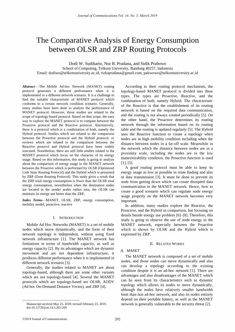
a) The Architecture of ZRP Network

Fig. 1 shows that the radius of the ZRP area. The

radius area of S node is structured by all nodes around it

which are A node, B node, C node, D node, E node, and

F node, including all other nodes which become

neighbors of the nodes around S node which are G node,

H node, I node, and J node which are determined as

border nodes [9]. K node is counted as the node which is

placed outside of S node radius area [9]. If the data

communication range is in the S node radius area then the

S node is going to use IARP mechanism for data

communication. In contrast, if the data communication

range cannot be reached by the S node radius area then

the S node is going to use IERP mechanism for data

communication [9].

S

The S node radius area

The network topology

A

B

C

D

E

F

H

I

K

J

G

Fig. 1. The architecture of ZRP network [9].

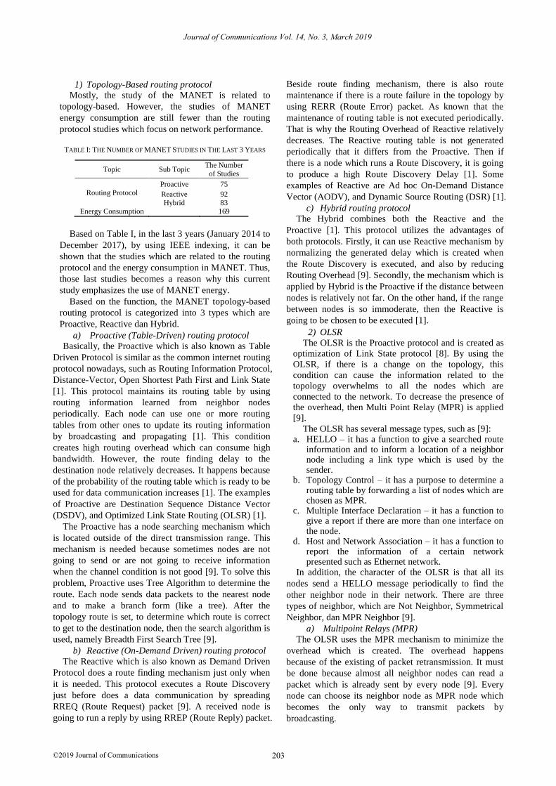
b) The Architecture of ZRP Components

The ZRP also implements Broadcast Routing Protocol

(BRP). This protocol is also applied to establish a list of

nodes (which is given by the IARP protocol) based on

routing information which is collected and to spread

searched route request between the zone (IERP) in the

network [9]. The way executed is by sending HELLO

beacon message in the certain time interval to find node

existence. Fig. 2 explains the architecture of ZRP

components.

Fig. 2. The architecture of ZRP components.

B. Network Simulator 2 (NS2)

Network Simulator 2 is an event-driven simulator

which is specifically designed for observing network

computer and data communication in the network [11].

NS2 is developed by using 2 programming languages

which are [11]:

1. C++ becomes the first. It is a library which contains event scheduler, protocol, including network component which is implemented by the user for the simulation. C++ is used as a library because it can support the simulation to run quickly, even the simulation uses very big number packets of data.

2. Tcl/Otcl is the second programming language which is used as a simulation script. It is written by a user, and it acts as an interpreter. On the other hand, Tcl gives a response if there is a syntax failure and if there is a script which changes suddenly.

The output result of NS2 simulation is a text-based file

which the format is .tr, and also an animation-based file

which the format is .nam. To interpret an output result as

an interactive graphic then tools which are NAM

(Network Animator) and Xgraph are used. To analyze a

user network behavior, the user can extract a relevant part

from the text-based result and can change it into other

form which can be understood easily.

1) The Consumption Energy of MANET

The energy usage in MANET network can be modeled

by simulated by using some models. The model then is

going to be used as the source to make a scenario of

MANET network simulation. There are several models

which are known based on preliminary studies such as [1]

[3]:

Network-Size Model – The size of topology network gives big influence to MANET network energy consumption, especially when Route Discovery process and multi-hop data transmission are executed. Even the network size can give an effect to the node consumption energy, but each MANET protocol has its mechanism to adapt to every change in the network [3].



Constant-Speed Model – Node speed also affects MANET network energy consumption. The faster the node, the bigger the energy consumption [3].

Floating-Speed Model – Node accelerating also gives an impact to MANET energy consumption. The bigger the accelerate, the bigger the energy used [3].

Pause-Time Model – When there is a node movement from a started point to a destination point, sometimes there is an interlude. The longer the interlude, the bigger the energy saving [3].

Different Node Density – If the number of MANET nodes become bigger, this condition can increase the energy consumption which is generated by every MANET network nodes [1].

Even there are several models for making the MANET

network simulation, this study is only going to compare

between the OLSR and the ZRP by using Network-Size

Model and Different Node Density as the modified

increasing of the sender and the receiver nodes.

2) Energy consumption model

Hence, the equation which can be used to calculate the

energy consumption of packets which are transmitted by

a node. It can be followed as [2]:

𝐸(𝑝) = 𝑖 ∗ 𝑣 ∗ 𝑡𝑝 (1)

which 𝑖 is an electric current, 𝑣 is an electric voltage, and

𝑡𝑝 is the time which is needed to transmit the packet 𝑝.

The unit which is applied to represent the energy used is

Joule [2].

III. PROBLEM DEFINITION

Generally, many studies about MANET are related to

protocol performance and its services in the computer

network. However, the number of studies which are

related to the energy consumption used by MANET

nodes are still rare.

The importance related to the observation of the

MANET energy consumption, especially in the ad-hoc

network, because the use of node energy is not spread to

every node in MANET network evenly. If the certain

nodes which have an important role to deliver packets use

very high energy precisely then this condition makes the

delivery process between the sender and the receiver is

going to be broken. Based on that information, the study

which is related to energy consumption in the MANET

network becomes crucial.

IV. PROPOSED METHOD

The first step in this study is to acquire the role of

OLSR and ZRP protocols to determine the best scenario

and the best topology for the simulation. There are

several models and parameters which can be used to

simulate both protocols. The parameters which are

applied in this study are related to both models, namely

Network-Size Model and Different Node Density. Both

models are used in order to know the energy consumption

used by the OLSR and the ZRP in the MANET network.

The network topology is designed which has relatively

wide area and has receiver nodes which their number

becomes bigger among the increased time. Based on the

models used, the focus of this study is stressed about the

energy of transmitters (sender nodes) and intermediate

nodes (channel nodes). It is going to be executed because

both types of nodes are assumed as the nodes which use

bigger energy than other types of nodes.

A. The Topology of MANET Network

The initial topology before the nodes move or just

before the simulation runs can be shown in Fig. 3. The

network consists of 20 nodes and the nodes consist of

sender nodes, channel nodes, and destination nodes.

S1

S2S3

S4

CH

1

CH

2

CH

3

CH

4

D2

D3D1

D5

D6

D4

D8

D7D9

D

11

D

10

D

12



Fig. 3. The initial nodes position before the simulation starts.

Fig. 3 presents the network topology which is used by

the simulation. There are several types of nodes which

are:

The type of sender nodes (S1-S4) which has a function as packet senders.

The type of channel nodes (CH1-CH4) which has a function to deliver data from sender nodes to destination nodes if it is needed.

The type of destination nodes (D1-D12) which has a function as packet receivers.

B. System Design

After the network topology is determined based on the

models which are chosen then the analysis of each

MANET node energy consumption is going to be

executed by using Network Simulator 2 (NS-2).

1) Initialisation

1. At the beginning of simulation, all nodes become

closer which are determined as Figure 3.

2. The sender nodes are located in the center of the

network topology. The channel nodes and also the

destination nodes move slowly to evade the sender

nodes.

3. The channel nodes are placed between the sender

nodes and the destination nodes. They deliver the

data from the sender nodes to the destination nodes

if the destination nodes area are seated outside of

sender nodes radius area.

4. Each nodes type has a different pace.

5. The delivery of packets uses UDP service. So that

the delivery service is going to be simulated by

using Constant Bit Rate (CBR).



6. The delivery of each packet is going to use 512

bytes per packet for transmission.

C. The Scenario of Simulation

In this study, the observation is done using 2 different

scenarios. The scenarios are analyzed based on the time

of simulation. The result of the simulation is analyzed

based on several factors such as the topology changes as

the impact of the destination nodes movement, including

the increasing number of destination nodes which receive

the packets from sender nodes.

The scenarios are executed to know about the energy

consumption used by MANET network, before and after

the network topology changes. The important point for

this simulation is that the change of the network topology

happens when the destination nodes just start to move

outside of the sender nodes radius area, and the channel

nodes just begin to deliver the packets from the sender

nodes to the destination nodes. This is the way to

calculate the energy used by each protocol which is

counted before the topology changes and after the

topology changes. After the results of the energy

calculation are collected, then the results are going to be

compared.

TABLE II: THE CONFIGURATION OF MANET NETWORK SIMULATION

Parameter Value

Simulation time 200 s

Dimension 1000 m × 1000 m

Wireless radio range 250 m The number of mobile node 20 nodes

Node speed 1-4 m/s

Traffic type (CBR) 512-byte per packet Initial energy 20 Joule

1) Scenario 1

In this scenario, the OLSR and the ZRP are simulated

in the condition which is the sender nodes send the

packets to the destination nodes without using the

channel nodes. So that in the initial network, the channel

nodes act not as an intermediate in the MANET network.

Then as the time goes on, the destination nodes move

outward away from the sender nodes. Similarly, the

channel nodes move outside from the sender nodes. So

that it is going to happen that the topology changes due to

the destination nodes out of the sender nodes radius area,

and finally the channel nodes are going to be used as

intermediary nodes to deliver the data packets from the

sender nodes to the destination nodes. The sender nodes

move at the low speed of 1 m/s in the close range, the

channel nodes migrate at the medium speed of 2 m/s, and

the destination nodes move at the speed of 4 m/s in the

farthest range. The simulation time adopted is 200 second

in order to explore how many energy used by each node

before and after the network topology changes.

When the network routing changes, the OLSR is going

to use the mechanism of Proactive. On the other hand, the

ZRP is going to use the operation of Reactive. The OLSR

is going to nominate the channel nodes (CH) as MPR

nodes to transmit the packets, and the ZRP is going to set

the border nodes to run using BRP protocol to minimize

the energy consumption when they deliver the packets

from the sender nodes to the destination nodes.

S1

S2S3

S4

CH

1

CH

2

CH

3

CH

4

D2

D3D1

D5

D6

D4

D8

D7D9

D

11

D

10

D

12



Fig. 4. The network topology used for scenario 1.

Fig. 4 exposes the final position of the network

topology for scenario 1. This scenario is going to use 20

nodes and the simulation is executed three times. As long

as the process repetition, the number of the destination

nodes (D) are going to be added. At the beginning, each

sender node (S) only send the packets just to one

destination node (D). Then the packets is going to be sent

repeatedly with the additional number of the receiver (D).

Finally, each sender node (S) send the packets to three

destination nodes (D) via the channel node (CH)

simultaneously.

2) Scenario 2

Fig. 5 exhibits the position of nodes when the network

routing still does not change. The sender nodes (S)

directly send the packets to the destination nodes (D)

without using the channel nodes (CH).

S1

S2S3

S4

CH

1

CH

2

CH

3

CH

4

D2D3D1

D5

D6

D4

D8D7D9

D

11

D

10

D

12



Fig. 5. The network topology used for scenario 2.

This scenario uses 20 nodes. Three times of simulation

are executed by adding the number of the destination

nodes (D) from one node to three nodes for each sender

node (S).



Based on the results of both scenarios, then the

calculation to estimate the energy needed when the

network routing changes can be done. The estimation can

be done by reducing the total energy used in the scenario

1 with the total energy used in the scenario 2. The

composition which is estimated is based on:

1. The total energy needed by all nodes.

2. The total electrical power required by all sender

nodes (S).

3. The total energy used by all channel nodes (CH).

V. ANALYSIS AND DISCUSSION

The calculation of energy needed is going to be

analyzed and it is going to be parted into three pieces

which are:

o Counting the energy consumption of MANET

network by using simulator from the beginning of the

time to the time 𝑡 = 200 second.

o Calculating the energy needed of MANET network by

using NS2 from the beginning of the time until the

end of time as long as the network routing does not

change.

o Estimating the energy needed of MANET network by

using NS2 simulator from the beginning of the

network routing just changes to the time 𝑡 = 200

second.

A. The Consumed Energy Calculation of the Network

from the Beginning of Time to the Time 𝑡 = 200

Second

In this part, the consumed energy of the OLSR and the

ZRP are going to be analyzed by using the range of time

between the time 𝑡 = 0 second and the time 𝑡 = 200

second. The energy calculated are the electrical power of

the sender and the channel nodes before and after the

topology changes including the changed number of the

destination nodes.

TABLE III: THE CONSUMED ENERGY RELATED TO THE NUMBER OF THE

DESTINATION NODES

The Energy Consumption (Joule)

OLSR ZRP

Node 1 (D) 2 (D) 3 (D) 1 (D) 2 (D) 3 (D)

S1 18.01 20 20 18.85 20 20

S2 18.04 20 20 18.83 20 20

S3 18.03 20 20 18.80 20 20

S4 18.02 20 20 18.82 20 20

CH1 15.95 18.03 16.44 16.46 16.27 15.34

CH2 15.99 18.01 16.31 16.41 17.11 15.17

CH3 15.99 17.91 16.35 16.48 17.39 15.75

CH4 15.98 17.88 16.69 16.50 17.07 15.44

Total (20 nodes) 272.11 295.38 289.91 283.55 294.45 289.43

As an explanation of Table III which is related to the

OLSR, when S1 node (the sender node) sends the packets

only to one destination node (D), it needs 18.01 Joule

energy. When S1 node sends the packets to two

destination nodes, it needs 20 Joule energy. So it goes on

continuously.

Based on the information of Table III, according to the

total energy needed by MANET network from the time 𝑡

= 0 second to the time 𝑡 = 200 second, it can be said that

the energy consumption of the OLSR is fewer than the

energy needed by the ZRP when the sender node only

transmits the packets to one destination node. However,

as the increasing number of the destination nodes which

receive the packets from the sender nodes, for all nodes,

the ZRP tends to be more efficient than the OLSR.

Fig. 6. The consumed energy related to the destination node.

Fig. 6 displays the comparison of the total energy

consumption between the OLSR and the ZRP in the range

of time between the time 𝑡 = 0 second and the time 𝑡 =

200 second.

B. The Consumed Energy Calculation of the Network

from the Beginning of Time to the Time Before the

Topology Just Changes.

In this part, the consumed energy of the OLSR and the

ZRP is going to be analyzed by using the scenario 2.

After the scenario 1 is finished executed, the value of

time 𝑡 before the network routing just changes is

collected.

The range of the OLSR time for run is fewer than the

range of ZRP time when both time ranges are collected

from the beginning until before the network routing just

changes. It can be said that the change of network routing

of the OLSR is faster than the change of network routing

of the ZRP. This condition can be understood because the

OLSR is more aggressive to update its routing table than

the ZRP, even though both protocols use the same

mechanism namely the Proactive.

Based on the simulation, it is gathered that the time

before the network routing just changes is at the second

of 79 for the OLSR, and is at the second of 86 for the

ZRP.

The energy consumption needed by the sender nodes

and the channel nodes of both protocols before the

network topology just changes can be seen on Table IV.

As an explanation of Table IV, according to the ZRP

protocol, when S1 node (the sender node) send the

packets to one destination node, it needs the energy of

8.03 Joule. Then, when the S1 node transmits the packets



to two destination nodes, it needs the energy of 10.49

Joule. So it goes on continuously.

For the Proactive mechanism which the destination

nodes (D) are located on the sender nodes (S) radius area,

the OLSR uses the energy consumption more efficient

than the ZRP. In this simulation, the channel nodes (CH)

is not being an intermediate between the sender nodes (S)

and the destination nodes (D). So that the energy

consumption of the channel nodes in the simulation just

for only the movement. So that, particularly, the focus in

this simulation just to compare the energy used by the

sender nodes (D) of both protocols.

TABLE IV: THE CONSUMED ENERGY RELATED TO THE NUMBER OF THE

DESTINATION NODES BEFORE THE TOPOLOGY JUST CHANGES


OLSR ZRP

Node 1 (D) 2 (D) 3 (D) 1 (D) 2 (D) 3 (D)

S1 6.89 9.53 12.16 8.03 10.49 13.04

S2 6.91 9.52 12,14 8.04 10.53 13.12

S3 6.91 9.57 11.9 7.96 10.49 13.02

S4 6.89 9.55 11.98 8.02 10.49 13.13

CH1 4.36 4.83 4.97 5.28 5.41 5.63

CH2 4.40 4.84 4.86 5.23 5.42 5.63

CH3 4.40 4.73 4.8 5.3 5.4 5.61

CH4 4.40 4.68 5.01 5.32 5.4 5.7

Total (20 nodes) 98.16 114.49 128.73 115.79 129.66 144.91

Even the focus of analysis just to compare the sender

nodes energy consumption of both protocols, however,

the trend of energy used shows similar trends with the

energy consumption of all nodes. The total of the energy

consumption which is related to the additional number of

the destination nodes before the network routing just

changes can be seen in Fig. 7.

Fig. 7. The consumed energy related to the destination node (before the

topology just changes).

Based on Fig. 7, it can be shown that the number of the

destination nodes which receive the packets affects the

energy consumption of MANET network for both

protocols even it is for the network topology which its

network routing does not change.

It can be seen that the bigger the number of the

destination nodes, then the bigger the energy

consumption needed.

In the scenario 2, the OLSR is more efficient for the

energy used than the ZRP. It happens because before the

topology changes, the destination nodes are still located

in the sender nodes radius area. Then the routing creation

of OLSR routing table is more efficient than the routing

generation of ZRP routing table.

C. The Consumed Energy Calculation of the Network

from the Beginning of Time to the Time 𝑡 = 200

Second

The calculation of the energy consumption when the

network topology just changes its network routing is

counted by reducing the total energy acquired of MANET

network in the first scenario with the total energy used of

MANET network in the second scenario.

Based on the simulation in the first scenario that the

time before the network routing just changes is at the

second of 79 for the OLSR, and is at the second of 86 for

the ZRP. Thus the calculation of the energy consumption

for the OLSR when the network topology just changes is

from the time 𝑡 = 80 to the time 𝑡 = 200. For the ZRP is

from the time 𝑡 = 87 to the time 𝑡 = 200.

TABLE V: THE CONSUMED ENERGY RELATED TO THE NUMBER OF THE

DESTINATION NODES AFTER THE TOPOLOGY JUST CHANGES


OLSR ZRP

Node 1 (D) 2 (D) 3 (D) 1 (D) 2 (D) 3 (D)

S1 11.12 10.47 7.84 10.82 9.51 6.96

S2 11.13 10.48 7.86 10.79 9.47 6.88

S3 11.12 10.43 8.1 10.84 9.51 6.98

S4 11.13 10.45 8.02 10.8 9.51 6.87

CH1 11.59 13.20 11.47 11.18 10.86 9.71

CH2 11.59 13.17 11.45 11.18 11.69 9.54

CH3 11.59 13.18 11.55 11.18 11.99 10.14

CH4 11.58 13.2 11.68 11.18 11.67 9.74

Total (20 nodes) 173.95 180.89 161.18 167.76 164.79 144.53

Based on Table V, it can be examined that the energy

needed by the ZRP network which utilizes the sender

nodes and the channel nodes is fewer than the OLSR

network. It happens because when the network routing

just changes, the ZRP uses the Reactive mechanism. On

the other hand, the OLSR still applies the Proactive

mechanism which needs more energy than the Reactive

mechanism.

The total energy consumption which is related to the

destination nodes after the network routing just changes

can be seen in Fig. 8.

Fig. 8. The consumed energy related to the destination node (after the

topology just changes).



Fig. 8 shows the values which are collected by

reducing the total energy consumption of MANET

network simulated in the scenario 1 with the total energy

consumption of MANET network simulated in the

scenario 2.

VI. CONCLUSIONS

Based on the simulation analysis which observes about

the energy consumption of the ZRP and the OLSR, it can

be examined that the OLSR which represents the

Proactive has the most efficient mechanism to deliver the

packets when the destination nodes are located in the

sender nodes radius area. It happens because the OLSR

can maintain the updated routing table more efficient than

the ZRP. It can be seen that the energy consumption

needed by the OLSR in the MANET network simulation

is fewer than the energy consumption used by the ZRP in

the MANET network simulation.

The ZRP which represents the Hybrid has the most

efficient mechanism to deliver the packets when the

destination nodes are located out of the sender nodes

radius area. It happens because the ZRP uses the Reactive

mechanism when the destination nodes are not placed in

the sender nodes radius area. It can be seen that the ZRP

energy consumption is fewer than the OLSR energy

consumption.

The ZRP which represents the Hybrid uses the

Proactive mechanism when the destination nodes are

located in the sender nodes radius area. However, the

updated mechanism of the ZRP routing table is not as

efficient as the updated mechanism of OLSR routing

table. It can be seen that the ZRP sender nodes energy

consumption is higher than the OLSR sender nodes

energy consumption.

By the way, as the increasing of the MANET network

density, the ZRP energy consumption tends to be more

efficient than the OLSR energy consumption. It can be

seen by examining the channel nodes energy

consumption and the destination nodes energy

consumption together.

All in all, the total energy consumption of the ZRP is

fewer than the OLSR, and it has the most efficient energy

consumption for transmitting packets for all simulation.

REFERENCES

[1] K. Nayak and N. Gupta, “Energy efficient consumption-

based performance of AODV, DSR and ZRP routing

protocol in MANET,” International Journal of

Engineering and Innovative Technology (IJEIT), vol. 4,

no. 11, pp. 82–90, 2015.

[2] J. C. Cano, “Investigating performance of power-aware

routing protocols for mobile ad-hoc networks,” in Int.

Mobil. Wirel. Access Work (MobiWac), 2002, pp. 80–86.

[3] J. H. Zhang, H. Peng, and F. J. Shao, “Energy

consumption analysis of MANET routing protocols based

on mobility models,” in Fuzzy Syst. Knowl. Discov.

(FSKD), 2011, pp. 2275–2280.

[4] V. A. Gajbhiye and R. W. Jasutkar, “Study of efficient

routing protocols for VANET,” Int. J. Sci. Eng. Res., vol.

4, no. 3, pp. 1–8, 2013.

[5] Vir, S. Agarwal, and S. Imam, “Investigation on aspects

of power consumption in routing protocols of MANET

using energy traffic model,” Int. J. Adv. Res. Electr.

Electron. Instrum. Eng., vol. 2, no. 1, pp. 590–598, 2013.

[6] P. Garnepudi, T. Damarla, J. Gaddipati, and D. Veeraiah,

“Proactive, reactive and hybrid multicast routing protocols

for wireless mesh networks,” in Proc. IEEE Int. Conf.

Comput. Intell. Comput. Res. (ICCIC), 2013, pp. 1–7.

[7] R. Ahuja, “Simulation-based performance evaluation and

comparison of reactive, proactive and hybrid routing

protocols based on random waypoint mobility model,” Int.

J. Comput. Appl., vol. 7, no. 11, pp. 20–24, 2010.

[8] M. Rahman, F. Anwar, J. Naeem, M. Abedin, and S.

Minhazul, “A simulation-based performance comparison

of routing protocol on mobile ad-hoc network (proactive,

reactive and hybrid),” Comput. Commun. Eng., 2010, pp.

1–5.

[9] Mohammed, C. Badr, and E. Abdellah, “Comparative

study of routing protocols in MANET,” in Proc. Int. Conf.

Next Gener. Networks Serv. (NGNS), 2014, pp. 149–153.

[10] S. Mittal and P. Kaur, “Performance comparison of

AODV, DSR and ZRP routing protocols in MANET’s,”

in Proc. Int. Conf. Adv. Comput. Control Telecommun.

Technol. (ACT), 2009, pp. 165–168.

[11] T. Issariyakul and E. Hossain, Introduction to Network

Simulator NS2, Springer Science & Business Media, 2011.

Dodi W. Sudiharto was born in Jakarta,

Indonesia, in 1976. He received the

Bachelor of Engineering from Department

of Electrical Engineering, University of

Indonesia (UI), Depok, Indonesia in 2001

and Master of Science in Information

Technology from Computer Science,

University of Indonesia (UI), Jakarta, Indonesia in 2004. His

research interests include Computer Network, Netcentric, and

Internet of Things (IoT).

Nur R. Pradana. He received Bachelor of Engineering from

School of Computing, Telkom University, Bandung, Indonesia

in 2018. His research interests include Computer Network and

its simulation.

Sidik Prabowo. He received Bachelor of

Engineering from Telkom Institute of

Technology, Bandung, Indonesia in 2011

and Master of Engineering from Telkom

University, Bandung, Indonesia in 2014.

His research interests include Machine to

Machine and Wireless Sensor Network.



the comparative analysis of energy consumption between

Documents