The Complementary Nature of Trust and Contract Enforcement

Björn Bartling, Ernst Fehr, David Huffman, and Nick Netzer*

January 18, 2021

Under weak contract enforcement the trading parties’ trust, defined as their belief in other’s trustworthiness, appears important for realizing gains from trade. In contrast, under strong contract enforcement beliefs about other’s trustworthiness appear less important, suggesting that trust and contract enforcement are substitutes. Here we show, however, that trust and contract enforcement are complements. We demonstrate that under weak contract enforcement trust has no effect on gains from trade, but when we successively improve contract enforcement, larger effects of trust emerge. Likewise, improvements in contract enforcement generate no increases in gains from trade under low initial trust, but cause high increases when initial trust is high. Thus, the effect of improvements in contract enforcement is trust-dependent, and the effect of increases in trust is dependent on the strength of contract enforcement. We identify three key ingredients underlying this complementarity: (1) heterogeneity in trustworthiness; (2) strength of contract enforcement affecting the ability to elicit reciprocal behavior from trustworthy types, and screen out untrustworthy types; (3) trust beliefs determining willingness to try such strategies. Keywords: Trust, contract enforcement, complementarity, equilibrium selection, causal effect, screening, belief distortions, institutions JEL: C91, D02, D91, E02

* Bartling, Fehr, Netzer: Department of Economics, University of Zurich, Blümlisalpstrasse 10, 8006 Zurich, Switzerland, e-mail: bjoern.bartling@econ.uzh.ch, ernst.fehr@econ.uzh.ch, nick.netzer@econ.uzh.ch. Huffman: Department of Economics, University of Pittsburgh, 4901 Wesley Posvar Hall, 230 South Bouquet Street, Pittsburgh, PA 15260, USA, e-mail: huffmand@pitt.edu.

2

1. Introduction Incomplete and imperfectly enforceable agreements are ubiquitous in economic life. Informational

constraints render it impossible in many cases to govern all conceivable contingencies in a contract

and to verify all enforcement-relevant information. Moreover, weak judicial systems render it

infeasible or extremely costly in many countries to enforce contractual promises even when

informational constraints are not binding.1 The contracting parties are therefore exposed to the

threat of being cheated and they may only be willing to interact and realize the associated gains

from trade if they trust that the other party will not take advantage of them. It has therefore been

argued that trust is of fundamental importance for achieving economic efficiency (see, e.g.,

Banfield, 1958; Arrow, 1972; Coleman, 1990; Putnam, 1993, 2000; Fukuyama, 1995). The scope

for trust to shape economic outcomes appears broad. Trust can affect individual-level economic

interactions, the efficiency of organizations, the functioning of entire markets, and even economic

development and growth at the country level.

It is quite evident that trust, which we define in this paper as people’s beliefs in the

trustworthiness of others, matters when contracts are incomplete or imperfectly enforceable. It is,

however, less clear and to the best of our knowledge an unstudied question whether trust and

contract enforcement are substitutes or complements for the realization of gains from trade.

Depending on the answer to this question, fundamentally distinct policy implications result. In this

paper, we study experimentally and theoretically the nature of the interaction of trust and contract

enforcement.

Intuitively, trust appears to be more important in environments with lower contract

enforcement because the scope for cheating on the trading partner is higher. Therefore, more trust

is required to initiate or execute a trade. Thus, if both trust and contract enforcement are causal

factors in the realization of gains from trade, it appears that a lower level of trust can be

compensated for by a higher level of contract enforcement, and vice versa, to achieve a given

realization of gains from trade. In other words, trust and contract enforcement would be substitutes

that can be varied independently to increase the realization of gains from trade. If this were true,

1 Djankov et al. (2008)—who study debt enforcement in 88 countries around the globe—report, for example, that a worldwide average of 48 percent of the asset’s value is lost in debt enforcement, and North (1991) suggests that lack of contract enforcement is one of the key obstacles to economic development.

3

policies aimed at improving economic performance could be effective if they focused solely on

formal institutions, for example seeking to improve the judicial system in order to enable better

contract enforcement—even if levels of trust remained low. Likewise, policies aimed at moving a

society out of a low-trust trap, such as public awareness campaigns that promote codes of conduct

or advertise role models of trustful business relations, could be effective—even if formal

institutions remained weak and ensured only very imperfect contract enforcement. If, however,

trust and contract enforcement were complements, the above policies might remain fairly

ineffective if pursued in isolation. Policies would then be more likely to be successful if they

simultaneously improve formal institutions that ensure better contract enforcement and raise trust

levels.

In this paper we report the results of controlled experiments which suggest that trust and

contract enforcement are complements for the realization of gains from trade. We show, in

particular, that an independent improvement in contract enforcement at low levels of trust

generates no or only small increases in gains from trade, while improvements in contract

enforcement cause large increases in the average gains from trade at high trust levels. Likewise,

our data indicate that an increase in trust leads to no improvement in the gains from trade if contract

enforcement is weak but to high increases in gains from trade when contract enforcement is strong.

Our results are based on the exogenous variation of trust and contract enforcement in a laboratory

experiment involving principals and agents who face profitable trading opportunities in an

experimental market. The key advantage of this approach is that it allows for a clean separation of

the effects of trust and contract enforcement and their interaction on the realized gains from trade.

What are the economic and psychological mechanisms that drive the complementarity

between trust and contract enforcement? To provide deeper intuitions into the underlying

mechanisms, we need to provide a bit more detail about the experiment.

Our experiment involves principal-agent interactions, where the principals make contract

offers in an experimental market by promising to pay a wage and requesting an effort level from

the agents, while the agents choose the actual effort level after they accepted an offer. The gains

from trade are increasing in effort, but there is a conflict of interest as higher effort benefits the

principal while being costly for the agent. In all of our treatments, the enforcement of effort is

imperfect because effort is not third party verifiable and thus not contractible. Subjects interact in

4

markets of seven principals and ten agents for 15 periods. In a given period, a match between a

principal and an agent occurs if an agent accepts a principal’s offer.

We implement variation in the contractual environment by varying the degree of contract

enforcement as follows. In our weak contracting environment, the principal can pay any wage to

the agent, irrespective of the wage that was promised in the contract.2 The principal and the agent

simultaneously choose the actual wage and actual effort after the agent accepted the contract. In

addition, the parties face an informational constraint that prevents them from making contracts

contingent on signals of past behavior. We implement this constraint by scrambling (i.e., re-

randomizing) the ID numbers of principals and agents across periods such that interactions remain

one-shot. In our medium contracting environment, we improve contract enforcement by rendering

the principals’ wage promises legally enforceable, i.e., the principal is forced to pay the promised

wage. Otherwise, this treatment is identical to the weak contracting environment. Our strong

contracting environment adds an additional improvement in contract enforcement by keeping

identification numbers the same across rounds. This allows principals to make their contract offers

contingent on signals about the agents’ previous effort choices.

We implement (and verify) variation in principals’ initial trust about the agents’

trustworthiness by showing the principals, before the start of the experiment, examples of real

historical effort choices in experimental sessions in which the agents either exhibit trustworthy

behavior (shown in our high-trust treatments) or untrustworthy behavior (shown in our low-trust

treatments). If the principals’ trust has a positive causal effect we should observe it by comparing

the high-trust treatments with the low trust treatments.

How do we explain our finding that the impact of trust actually depends on strength of

contract enforcement, and vice versa? Our investigation of mechanisms suggest three key

ingredients: (1) heterogeneity in agents’ trustworthiness; (2) an impact of contract enforcement on

the ability of principals to elicit high efforts from trustworthy agents, and to distinguish trustworthy

from untrustworthy agents and engage in reciprocal relationships with the former; (3) an impact

of principals’ initial trust on their willingness to try such strategies.

2 This contracting environment may reflect a weak or inefficient judicial system—as is often the case in developing countries—or informal contracting with merely verbal promises. In developing countries a large share of workers, sometimes even a majority, is employed casually in the informal sector (Banerjee and Duflo 2007, La Porta and Shleifer 2014, McCaig and Pavcnik 2015).

5

Regarding the first ingredient, a large experimental literature indicates that there is

heterogeneity in trustworthiness, and our data are in line with this as well. Previous studies have

shown that many agents are trustworthy, in that they are willing to reciprocate with high effort if

they are offered high, generous wages that not only cover their cost but also give them a fair share

of the available surplus. While a significant share of subjects have social preferences that imply

such reciprocal, fairness-motivated responses, the literature also shows that there is typically a

significant share of relatively selfish subjects who are untrustworthy in that they show only weak

or no preference for fairness or reciprocal behavior (e.g., Konow, 2000, 2003; Fehr and Schmidt,

1999; Bolton and Ockenfels, 2000; Charness and Rabin, 2002; Cappelen et al., 2007, 2013). Our

data also show signs of a mix of reciprocal and selfish behaviors of agents: If agents receive low

wages before making their effort choices, almost all choose low efforts, but if they receive higher

wages, there emerges substantial heterogeneity, with some agents choosing minimum effort

(untrustworthy) but others responding with high effort levels (trustworthy).

Against this backdrop of heterogeneity, it turns out that the strength of the contracting

environment affects the ability of principals to elicit high efforts from the reciprocal agents, thus

generating high gains from trade. Under weak contracting, while principals typically promise to

pay high wages, this is not contractually enforceable, and indeed principals rarely live up to their

promises and actually pay very low wages. The agents quickly anticipate that they cannot rely on

the principals’ promises and, therefore, even reciprocal agents show little willingness to respond

to high offered wages with high effort. As a consequence, the principals also have little reason to

keep their promises because if they keep them they experience no return. In other words, the lack

of legal enforcement of wage promises undermines agents’ reciprocal behavior and generates a

“low wage – low effort” equilibrium.

In the final part of the paper we present a theoretical model that captures key features of

our experimental game, and heterogeneity in agent types, in a simplified way. The model explains

the above described empirical regularities of our weak contracting environment. It shows that the

“low wage – low effort” equilibrium is unique, and predicts, in particular, that an exogenous shock

to the principals’ beliefs about the agents’ trustworthiness has no effects on wages, effort and gains

from trade—which is what we observe in this contracting environment.

The legal enforcement of the principals’ wage promises in our medium contract

environment constitutes a major improvement in contract enforcement because the principals can

6

now credibly commit themselves to high wages. The agents therefore know that a high wage

promise indeed offers them a generous share of the surplus, which prompts reciprocal agents to

respond to higher wages with higher effort levels. Because our high-trust manipulation generates

optimistic beliefs about the agents’ trustworthiness, in the sense that principals believe that agents

honor high wages with high effort, while in our low-trust manipulation they believe in a weaker

reciprocal response, the principals have a reason to pay higher wages in the high- compared to the

low-trust condition—which is confirmed by the data. Reciprocally motivated agents then respond

with higher effort levels in the high- compared to the low-trust condition, which explains the

positive average trust effect on gains from trade in the medium contracting environment.

Is the trust effect on the gains from trade in the medium contracting environment stable,

i.e., an equilibrium phenomenon? Or is it due to a transitory effect of changing the principals’

initial beliefs about the agents’ trustworthiness? To answer this question, we need to examine

whether the principals benefitted on average from paying high wages in the high-trust

environment. It turns out that this is not the case, i.e., the agents’ effort increase in response to a

wage increase is insufficient to render the wage increase profitable on average; this modest average

response reflects agent heterogeneity, with some agents having a strong response, but others

choosing minimal effort regardless of the wage. Paying higher wages in the high-trust environment

is not profitable on average, but the principals learn this only slowly over time. This learning

process is indicated by the fact that wage offers in the high-trust condition are decreasing and

towards the end they are so low that the agents provide statistically indistinguishable effort levels

in the high- and the low-trust condition of the medium contracting environment.

Our theoretical model rationalizes the transitory nature of the increase in the gains from

trade in the medium contracting environment. The model shows that if the agents’ reciprocal effort

responses are insufficiently strong (e.g., because the share of reciprocally motivated agents is too

small) there is still a unique “low wage – low effort” equilibrium. However, the model also predicts

that initially false (i.e., too optimistic) beliefs of the principals about the agents’ trustworthiness

induce the principals to make initially too high wage offers.

Finally, we show that there is a large and stable trust effect on agent efforts, and thus the

gains from trade, in our strong contracting environment. In addition to making credible wage

promises, principals can also condition their current contract offers on the agents’ past

performance signals in this environment. Principals can do this by making no offer, or an offer

7

with a lower wage to agents with low previous performance signals, and by targeting high wage

offers to agents with high previous performance signals. Empirically, principals in the high-trust

condition indeed screen agents in this way and target their high wage offers to agents who

previously signaled their trustworthiness; therefore, the wage-effort relation is substantially

steeper in the strong compared to the medium contracting environment. This in turn means that

high wages can be profitable. In the low-trust condition, however, the principals believe that the

wage-effort relation is relatively flat and, therefore, make only low wage offers right from the

beginning, choosing not to try to screen for agents who respond to high wages with high efforts.

These wage differences between the high and the low trust condition are large and stable over time

and induce large and stable effort differences based on the agents’ reciprocal effort responses.

Our theoretical model rationalizes these findings because it shows that there coexist a high-

trust screening equilibrium, and a low-trust pooling equilibrium in the strong contracting

environment. The initial variation in the principals’ trust causes stable variation in the realized

gains from trade by selecting between these equilibria.

Our paper makes several contributions to the literature. First, it documents experimentally

that the effects of improvements in contract enforcement on gains from trade are trust-dependent.

To our knowledge, this is a novel empirical finding that may generally be interesting for the

economics of contracts and institutions (e.g., Bolton and Dewatripont, 2005; North, 1991) and, in

particular, for behavioral contract theory that examines the effects of non-standard motives and

social norms on the functioning of contracts and incentives (e.g., Ellingsen and Johannesson, 2005,

2008; Sliwka, 2007; Hart and Moore, 2008; Hart, 2009; Hart and Holmström, 2010; Herweg and

Schmidt, 2015; Bierbrauer and Netzer 2016; Danilov and Sliwka, 2017; Sliwka and Werner, 2017).

In addition, our findings on the role of trust in our strong contracting environment are also of

interest for the literature on relational contracting (e.g., MacLeod and Malcomson, 1998;

MacLeod, 2007; Gibbons, 1998; Baker et al., 2002; Gibbons et al., 2020).

Second, it clarifies the conditions under which we can expect a causal effect of trust on

gains from trade, and it shows the important role of the contracting environment in the transmission

of initial trust differences on wages, efforts, and gains from trade. Our paper thus contributes to

the debate on the effect of trust on economic outcomes (e.g., Knack and Keefer, 1997; La Porta et

8

al., 1997; Guiso et al., 2009; Algan and Cahuc, 2010; Bloom et al., 2012) by clarifying when we

can expect no, only transitory, or stable and large long run effects of changes in trust.3

Third, by empirically showing conditions for the emergence of a stable and efficient

reciprocal principal-agent interaction, our paper is also related to the literature on reciprocal gift

exchange and trust using laboratory experiments (Fehr et al., 1993; Berg et al., 1995; Brown et al.,

2004; Charness, 2004). Previous papers in the gift-exchange literature and more recent papers on

the counterproductive effects of sanctions and other measures that constrain shirking by agents

suggest that trust might be self-confirming (e.g., Bohnet et al., 2001; Bohnet and Huck, 2004; Falk

and Kosfeld, 2006; Bartling et al., 2012). However, this literature does neither address the

interaction of exogenous variations in trust and contract enforcement, nor does it identify the

conditions or mechanisms under which we should expect that trust affects trading efficiency.

Finally, our paper offers a simple theoretical model that captures the main empirical

regularities in our experiment and thus facilitates a coherent interpretation of the data. The model

rationalizes, in particular, why an exogenous increase in trust has no effect on gains from trade in

the weak contracting environment, only a transient effect in the medium contracting environment,

and a stable effect in the strong contracting environment.

The theoretical literature has shown before that different levels of trust can arise in a given

economic environment due to multiple equilibria (e.g., Tabellini, 2008; Aghion et al., 2010) or

multiple stable long-run outcomes of dynamic learning processes (e.g., Bower et al., 1996). Our

experiment provides a first explicit test of the general idea that trust can play a role due to multiple

equilibria: the empirical result that an exogenous increase in trust has no stable effect in a unique

equilibrium environment but leads to stable effects in a multiple equilibrium environment

demonstrates this point. Our theoretical model, however, differs from the existing literature in two

important ways. First, we follow a standard game-theoretic approach with fixed preferences, while

Tabellini (2008) and Aghion et al. (2010) study behavior that is transmitted from generation to

generation and coevolves slowly with external institutions. Our theoretical and empirical results

show that trust is malleable rather quickly and can have immediate and stable causal effects even

with fixed preferences and institutions. Second, in models like Bower et al. (1996), where agents

3 Our paper varies trust exogenously and examines the consequences of trust. There is also a literature that studies the individual and collective determinants of trust (e.g. Alesina and LaFerrara 2000 and 2005). For a review of the literature on the determinants of trust see Fehr (2009).

9

learn about a given population state, long-run levels of trust and economic efficiency cannot be

manipulated by interventions that select between different equilibria. By contrast, we show that

selecting the right equilibrium is an important consideration in the design of organizations and

mechanisms. This idea has also recently played an important role in organizational econonomics

where it has been argued that a deeper understanding of the forces that enable organizations to

“build” a more efficient equilibrium is key in understanding why some organizations persistently

perform better than others (Gibbons and Henderson, 2012; Gibbons, 2020; Gibbons et al., 2020).4

The remainder of the paper is organized as follows. Section 2 explains our experimental

design and contains a manipulation check showing that our exogenous variation of trust is

effective. Section 3 presents our main empirical finding on the complementary nature of trust and

contractual enforcement. Section 4 reveals the behavioral mechanisms behind our main empirical

findings by analyzing in detail how differences in the contractual environment shape the behavior

of principals and agents. Section 5 presents our theoretical analysis of the principal-agent game,

which helps us interpret and understand the empirical patterns described in the previous sections.

Section 6 concludes.

2. Experimental Design We study the impact of an exogenous variation in principals’ beliefs about the trustworthiness of

agents on wages, effort and gains from trade. To study the interaction between exogenous changes

in principals’ trust and the contract enforcement environment, we also vary the degree to which

parties can enforce contracts. We adopt a typical principal-agent framework where a higher effort

level by the agent increases the principal’s expected payoff but providing higher effort is more

costly for the agent. Principals and agents interact in an experimental market and we allow for 15

market periods, so that we can study how wages, effort and gains from trade evolve over time.

This feature make it possible to study whether exogenous changes in trust or contract enforcement

have stable or only transitory effects.

In our design, principals cannot directly observe effort levels but they receive an

informative stochastic signal about the agents’ effort choices, and higher effort levels are

4 In this context, the complementarity between trust and contract enforcement (i.e., incentives) is also important. Our findings suggest that to reap the available gains from trade it sometimes needs a change in incentives and a change in trust.

10

associated with an increase in the probability of observing a high signal. In many types of

economic interactions it is not possible to precisely identify whether effort or (bad) luck is

responsible for the observed output. The effort signal is observable by the principal and the agent,

but it is not verifiable by third parties and thus not directly contractible. Contracts are therefore

necessarily incomplete and the effort choice of an agent cannot be legally enforced. The principal’s

belief that an agent is trustworthy may then be relevant for the principal’s willingness to enter a

trade with an agent and for the contract terms the principal offers. We define agents to be

trustworthy when they are willing to reciprocate a high wage offer with a high effort choice

although high effort reduces their material payoff. Untrustworthy agents, by contrast, always

choose low effort levels irrespective of the offered wages.

Our treatments vary the degree to which the parties can enforce their agreement. In all

treatments, the principal proposes a contract that offers a wage and requests an effort level from

the agent. In the “weak contract enforcement” environment (WEAK), however, neither the offered

wage nor the requested effort level is legally enforceable. This environment thus represents a

situation with weak legal institutions. Furthermore, the identities of principals and agents are not

observable, and thus contract terms cannot be conditioned on the agent’s past performance signal.

In the “medium contract enforcement” environment (MEDIUM) we increase the scope for contract

enforcement by making the principals’ wage offers legally binding but the agent is still free to

choose any effort level, and it is still not possible to make contracts contingent on past performance

signals. In our “strong contract enforcement” environment (STRONG), principals’ wage offers are

again legally binding and agents are still free to choose any effort, but the subjects now have fixed

identification numbers over the course of the experiment. Principals can therefore target their

offers to specific agents contingent on their past performance signals, which is a further expansion

of the set of contractible contingencies relative to the other treatments.

2.1 Stage Game Payoffs If a principal and an agent agree to trade, then the principal pays a wage 𝑤𝑤 ∈ {1, … ,100} to the

agent and the agent chooses an effort level 𝑒𝑒 ∈ {1, … ,9}. The agent’s effort choice stochastically

determines the value of the interaction for the principal. There are only two possible value levels,

100 and 10. The probability that the principal receives the high value is given by 𝑒𝑒/10, while the

11

principal receives the low value with probability 1 − 𝑒𝑒/10. The expected material payoffs of

principals are thus given by

𝐸𝐸�Π𝑝𝑝𝑝𝑝𝑝𝑝𝑝𝑝𝑝𝑝𝑝𝑝𝑝𝑝𝑝𝑝𝑝𝑝� = �100 ∙ 𝑒𝑒10

+ 10 ⋅ �1 − 𝑒𝑒10� − 𝑤𝑤

0 if principal and agent interact

otherwise (1)

Π𝑝𝑝𝑎𝑎𝑒𝑒𝑝𝑝𝑎𝑎 = �𝑤𝑤 − 𝑐𝑐(𝑒𝑒)5

if principal and agent interactotherwise

(2)

where 𝑐𝑐(𝑒𝑒) denotes the agent’s cost of providing effort. The outside option of an agent who does

not interact with a principal is 5. Table 1 shows the cost function 𝑐𝑐(𝑒𝑒). The cost function is strictly

increasing and exhibits weakly increasing marginal costs. Since the marginal cost of effort is at

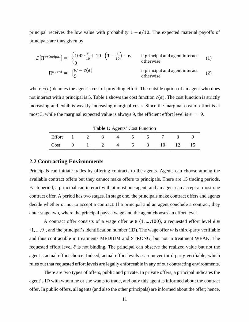
most 3, while the marginal expected value is always 9, the efficient effort level is 𝑒𝑒 = 9.

Table 1: Agents’ Cost Function

Effort 1 2 3 4 5 6 7 8 9 Cost 0 1 2 4 6 8 10 12 15

2.2 Contracting Environments Principals can initiate trades by offering contracts to the agents. Agents can choose among the

available contract offers but they cannot make offers to principals. There are 15 trading periods.

Each period, a principal can interact with at most one agent, and an agent can accept at most one

contract offer. A period has two stages. In stage one, the principals make contract offers and agents

decide whether or not to accept a contract. If a principal and an agent conclude a contract, they

enter stage two, where the principal pays a wage and the agent chooses an effort level.

A contract offer consists of a wage offer 𝑤𝑤 ∈ {1, … ,100}, a requested effort level �̃�𝑒 ∈

{1, … ,9}, and the principal’s identification number (ID). The wage offer 𝑤𝑤 is third-party verifiable

and thus contractible in treatments MEDIUM and STRONG, but not in treatment WEAK. The

requested effort level �̃�𝑒 is not binding. The principal can observe the realized value but not the

agent’s actual effort choice. Indeed, actual effort levels 𝑒𝑒 are never third-party verifiable, which

rules out that requested effort levels are legally enforceable in any of our contracting environments.

There are two types of offers, public and private. In private offers, a principal indicates the

agent’s ID with whom he or she wants to trade, and only this agent is informed about the contract

offer. In public offers, all agents (and also the other principals) are informed about the offer; hence,

12

each agent has the chance to accept a public offer. A principal can make as many private offers

and as many public offers as he or she wants in a given period. However, once an agent accepts

one of the offers, the principal is matched with this agent, learns the ID of the matched agent

(which is new information in case of a public offer), and his other outstanding offers are removed

from the market.5 The default at the beginning of each period is that no agent has a contract and

no principal has made an offer. There are always ten agents and seven principals in a market, i.e.,

there is an excess supply of three agents.

At the end of each period, each subject is informed about the own payoff and reminded of

the contract (𝑤𝑤, �̃�𝑒) he or she had concluded and the trading partner’s ID. Agents are also informed

about the payoff of their respective principal. Principals are not informed about the payoff of their

respective agent, because a principal does not observe the agent’s effort choice and thus the cost

of providing this effort level. The subjects write this information on a printed form that is provided

along with the experimental instructions. This procedure ensures that each subject can always

remind herself about her own trading history.

2.2.1 Contracting Environment WEAK

An agent can choose any actual effort level 𝑒𝑒 ∈ {1, … ,9} after having accepted a contract offer in

our contracting environment WEAK, irrespective of the requested effort level �̃�𝑒. Likewise, the

principal can pay any wage to the agent, irrespective of the offered wage. Actual wages and effort

levels are chosen simultaneously at the second stage of a period. Moreover, the subjects’

identification numbers (IDs) are randomly reshuffled in each of the 15 periods of the experiment

in contracting environment WEAK. Random IDs preclude the principals from conditioning future

contract offers on past performance signals. Neither of the two contracting parties thus faces legal

or economic incentives to stick to the terms of the contract in contracting environment WEAK,

but intrinsic motivation or social preferences could still induce them to honor their mutual

promises.

5 To prevent principals from making private offers to agents who have already concluded a contract with another principal, principals are at all times informed about which agents remain in the market.

13

2.2.2 Contracting Environment MEDIUM

A principal is obliged to pay the offered wage if an agent accepts his or her contract offer in our

contracting environment MEDIUM. An agent, however, can still choose any actual effort level

𝑒𝑒 ∈ {1, … ,9}, irrespective of the requested effort level �̃�𝑒. Principals must thus stick to the terms of

the contract in contracting environment MEDIUM while agents face no legal or economic

incentives to provide the requested effort level. Because IDs are still randomly shuffled in every

period, as in contracting environment WEAK, principals cannot condition hiring and contract

terms on signals about the past performance of specific agents.

2.2.3 Contracting Environment STRONG

Contract enforcement is strengthened further in our contracting environment STONG. The

principal is obliged to pay the offered wage 𝑤𝑤 if an agent accepts the contract, as in contracting

environment MEDIUM. Moreover, while agents can still choose any actual effort level 𝑒𝑒 ∈

{1, … ,9}, irrespective of the requested effort level �̃�𝑒, IDs of all players are fixed in our contracting

environment STONG. This feature provides principals with the opportunity to condition their

contract offers on the identity of a specific agent and this agent’s past effort signals. This provides

principals with the ability to screen agents and selectively target high wages to those who have

high past performance signals.6

2.3 Inducing Variation in Principals’ Trust To potentially induce exogenous variation the principals’ initial trust levels, we randomly assigned

them to two different information conditions. In the high-trust treatments, the principals were

informed about a “historical example” in which agents behaved in a trustworthy manner; in the

low-trust treatments, they were shown an example in which agents displayed a low level of

trustworthiness. More specifically, for our high-trust treatments we selected the market from

Brown et al. (2004) that had the steepest wage-effort relation, and for the low-trust treatments we

selected the market with the flattest wage-effort relation.

6 The idea of inducing one shot play by re-randomizing ID numbers every period and enabling long-run relationships by (i) fixing ID numbers throughout the experiment and (ii) allowing for private offers to specific agents is taken from Brown et. al. (2004). Their paper does however not vary exogenous trust levels and thus cannot study the interaction between the strength of contract enforcement and trust.

14

The example was provided at the end of the experimental instructions. Subjects were

informed that the information provided was an “example,” and that it showed how effort is related

to wage levels “in a past session.” Subjects were told that the information in the example was

something that they “could use in their decisions today.” The description of the source of the

example was completely truthful but deliberately vague, and we did not claim that the information

provided about a single past session was representative.

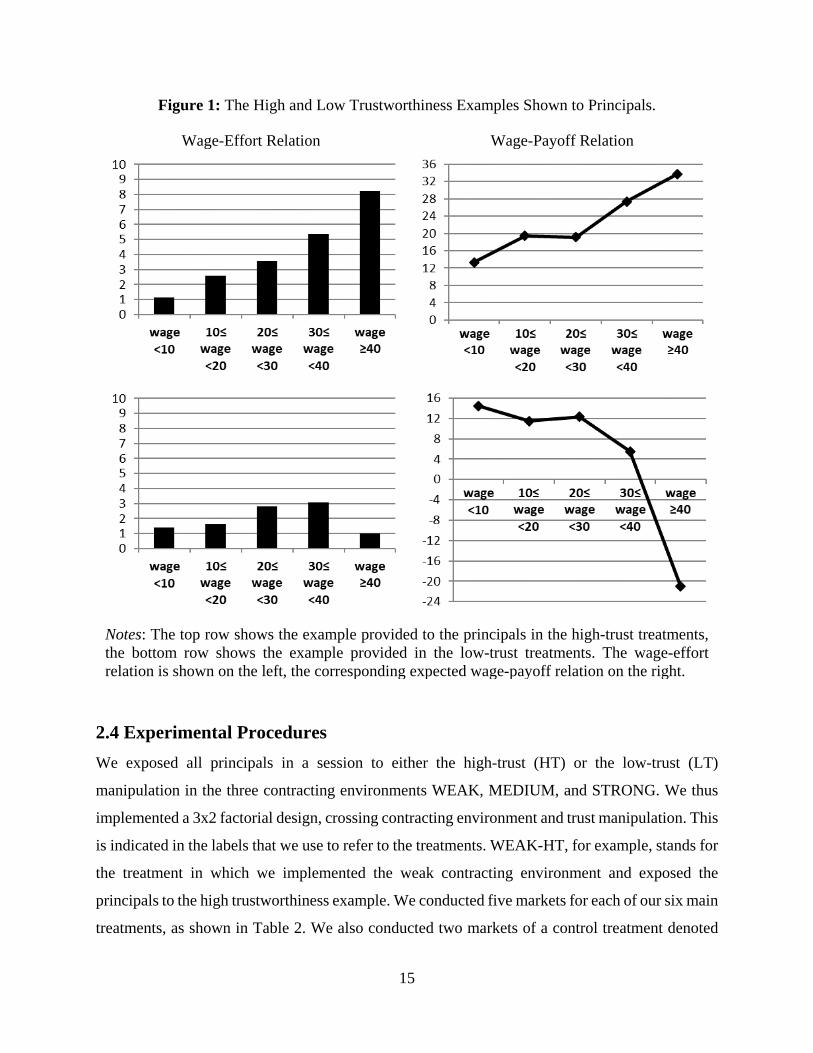
Figure 1 shows how we presented the examples to the subjects in the instructions. The top

row was shown to the principals in the high-trust treatments, the bottom row to the principals in

the low-trust treatments. On the left, the wage-effort relation is shown. The figure shows the

average effort provided by the agents in the example for each of the given bins of offered wages.

On the right, we show how this wage-effort relation translates into a wage-payoff relation, given

the principals’ payoff function in our experiment. The high trustworthiness example involved

agents being trustworthy, in that those who are paid high wages also exert high effort levels. In the

low trustworthiness example, agents were untrustworthy; they provided rather low effort for all

wage levels.

Note that the examples contain no information about the historical frequency of wage

choices by principals. They do indicate the range of wages that was used, but this was identical

across the high and and low trustworthiness examples. This is deliberate because we wanted to

rule out that the examples influence behavior by conveying information about historical behavior

of principals. Rather, the differential information content across examples is solely about the

trustworthiness of agents. Any impact should thus come through the beliefs of principals about

trustworthiness. We will examine in Section 2.5 the extent to which our trust manipulation was

effective in the sense that it differentially affected principals’ beliefs.

Subjects in the role of agents did not receive any example, nor were they informed that the

subjects in the role of principals received such information. The instructions for agents did not

differ in the high- and low-trust treatments, which rules out any direct impact on outcomes through

an influence on agents. This illustrates the advantages of an experimental setting for varying only

the principals’ trust, defined as the principals’ beliefs in the trustworthiness of the agents.

15

Figure 1: The High and Low Trustworthiness Examples Shown to Principals.

Wage-Effort Relation Wage-Payoff Relation

Notes: The top row shows the example provided to the principals in the high-trust treatments, the bottom row shows the example provided in the low-trust treatments. The wage-effort relation is shown on the left, the corresponding expected wage-payoff relation on the right.

2.4 Experimental Procedures We exposed all principals in a session to either the high-trust (HT) or the low-trust (LT)

manipulation in the three contracting environments WEAK, MEDIUM, and STRONG. We thus

implemented a 3x2 factorial design, crossing contracting environment and trust manipulation. This

is indicated in the labels that we use to refer to the treatments. WEAK-HT, for example, stands for

the treatment in which we implemented the weak contracting environment and exposed the

principals to the high trustworthiness example. We conducted five markets for each of our six main

treatments, as shown in Table 2. We also conducted two markets of a control treatment denoted

16

STRONG-HT-Long, which is identical to STRONG-HT, except that the game lasted 25 periods

rather than 15 periods. We use STRONG-HT-Long to clarify the possible role of end-game

effects7.

Table 2: Treatment Overview

Treatment Principals’ Wage Offers

Identification Numbers

Trustworthi-ness Example

# Periods

# Markets

WEAK-LT non-binding random low 15 5 WEAK-HT non-binding random high 15 5 MEDIUM-LT binding random low 15 5 MEDIUM-HT binding random high 15 5 STRONG-LT binding fixed low 15 5 STRONG-HT binding fixed high 15 5 STRONG-HT-Long binding fixed high 25 2

We implemented a between-subjects design, i.e., each subject participated in only one

market in one treatment. Altogether we have 32 markets, with seven principals and ten agents

each. Hence, 544 subjects participated in our experiment. Subjects were mainly students from the

University of Zurich and the Swiss Federal Institute of Technology in Zurich. Students majoring

in economics or psychology were not eligible to participate.

All sessions took place at the computer laboratory of the Department of Economics at the

University of Zurich. The study was computerized with the software z-Tree (Fischbacher, 2007)

and the recruitment was conducted with the software ORSEE (Greiner, 2015). Before the subjects

entered the lab, they randomly drew a place card that specified at which computer terminal to sit.

The terminal number determined a subject’s role as either principal or agent, which remained fixed

throughout the experiment.

7 Endgame effects reliably occur in finitely repeated cooperation games such as the prisoner’s dilemma and can typically be shifted into the future with a longer finite horizon (Embay, Frechette, Yuksel 2019). Similar effects can be observed in finitely repeated gift exchange experiments (see e.g., Brown, Falk and Fehr 2004). Thus, we conjectured that we will also observe an endgame effect in treatment STRONG-HT. Because we are interested in the stable effects of trust in STRONG-HT (i.e., in periods in which the endgame effect is not operative), we wanted to examine whether we can extend the effect of exogenous increases in trust by simply increasing the number of periods.

17

Subjects received written instructions including comprehension questions, which had to be

answered correctly before a session could begin.8 A summary of the instructions was read aloud

by the experimenter to generate common knowledge of the instructions. There were also two

practice periods before the actual experiment to make the subjects familiar with the market

procedures. Subjects only went through the first stage of the experiment in both practice periods,

so that principals did not observe payoffs and could not draw inferences about agents’ actual effort

choices. No money could be earned during the two practice periods.

Sessions lasted about 2.5 hours. Payoffs from the experiment, denominated in points, were

converted into money at the rate of 10 points to CHF 1 (about $ 1.05 at the time of the experiments)

at the end of a session. On average, subjects earned about CHF 47.65, which includes a show-up

fee of CHF 20. The subjects received their payments privately.

2.5 Manipulation Check Our experimental approach aims at potentially inducing exogenous variation in the principals’

beliefs about the agents’ trustworthiness. Figure 2 provides a manipulation check by showing the

principals’ expectations about the empirical relationship between offered wages and chosen effort.

These expectations were elicited at the beginning of the experiment, after reading the instructions

but before entering the trading periods. We asked principals to predict what they thought would

be the average effort level chosen by agents, conditional on different possible offered wages.

The figure reveals exogenous belief variation in all contracting environments, WEAK-HT

vs. WEAK-LT, MEDIUM-HT vs. MEDIUM-LT, and STRONG-HT vs. STRONG-LT. Principals

expected significantly higher average effort levels across the range of wages when they had

received the high trustworthiness example rather than the low trustworthiness example, and also

expected significantly steeper relationships between wage and effort. Regressions confirm that the

differences in average expected effort across the high and the low trustworthiness example were

statistically significant at the 1-percent level, as were the differences in slopes, in all three

8 We provide the experimental instructions in the appendix to this paper. Since the terms “principal” and “agent” are not in common usage among student subjects, the experiment was framed in terms of “buyers” and “sellers,” and we spoke about “price” and “quality” instead of “wage” and “effort.”

18

treatment pairs.9 On the other hand, we cannot reject the hypotheses that the average expected

effort, and the slopes of the wage-effort relations, are identical when comparing across treatments

involving the low trustworthiness example, and across treatments involving the high

trustworthiness example.10

Figure 2: Manipulation Check

Notes: The black lines show the wage-effort relation that principals expect in the three high-trust treatments WEAK-HT, MEDIUM-HT, and STRONG-HT. The grey lines show expectations in the three low-trust treatments WEAK-LT, MEDIUM-LT, and STRONG-LT. Since the agents do not receive historical examples about agents’ trustworthiness in a

previous experiment, random assignment should result in no differences in agents’ beliefs across

treatments involving high versus low trustworthiness examples. Indeed, we cannot reject the

9 The results for average expected effort are from OLS regressions of principals’ expectations about effort on the relevant treatment dummy, clustering standard errors at the subject level. All treatment dummy coefficients are significant at the 1-percent level. Results for the differences in slopes are from OLS regressions of expected effort on the relevant treatment dummy, the offered wage, and an interaction term, clustering on subject. All coefficients of the interaction terms are significant at the 1-percent level. 10 The results are based on OLS regressions of principals’ expectations about effort on the appropriate treatment dummies and interaction terms, clustering standard errors at the subject level.

19

hypothesis that the agents’ expectations about average effort, and the slope of the wage-effort

relations, are identical within each of the treatment pairs.11 Since the agents indicate their

“homegrown” beliefs, we can compare these beliefs with the beliefs that the principals indicate.

We find that the principals’ beliefs in the high-trust treatments roughly correspond to the agents’

homegrown beliefs. Principals who received the low trustworthiness example thus have beliefs

that are more pessimistic than homegrown beliefs.

3. The Complementarity of Trust and Contract Enforcement In this section, we present our main result on the complementarity between trust and contract

enforcement for the expected gains from trade. Figure 3 shows the average effort level in our three

contracting environments, comparing the high-trust and the low-trust conditions. Effort is a

sufficient statistic for the expected gains from trade, as higher effort levels directly generate higher

average gains from trade.

Figure 3: Expected Gains from Trade

Notes: Effort is a sufficient statistic for expected gains from trade. The black line shows the average effort in the high-trust environment in treatments WEAK, MEDIUM, and STRONG. The grey line shows the respective average effort in the low-trust environment.

11 The results are based on OLS regressions of agents’ expectations about effort on the appropriate treatment dummies and interaction terms, clustering standard errors at the subject level.

20

First, Figure 3 reveals that an exogenous increase in trust has no effect in contracting

environment WEAK, where principals are not obliged to pay the promised wage. This is in our

view an interesting finding because it indicates that under weak legal and economic contract

enforcement institutions, higher trust alone cannot increase trading efficiency.

Second, the figure reveals that the effect of trust on the expected gains from trade is positive

under improved contract enforcement conditions. The causal effect of trust is positive and

statistically significant in contracting environment MEDIUM, where the principals are

contractually obliged to pay the offered wage (Wilcoxon rank-sum test of market averages;

p<0.02).12

Third, the figure shows that the effect of trust is largest in contracting environment

STRONG. Corresponding regressions show that the differences in the impact of trust are

significantly different across the institutional environments (for MEDIUM vs. STRONG this is

true excluding an end-game effect in STRONG, which we discuss in more detail later).13

Figure 3 also shows that the effect of exogenous improvements in the contracting

environment are strongly trust-dependent. While improvements in contract enforcement induce a

large increase in expected gains from trade in the high-trust environment, much smaller (if any)

effects are observed in the low-trust environment. This again indicates the strong complementarity

between trust and the legal/economic contract enforcement environment for trading efficiency. It

is not sufficient to merely improve the contract enforcement environment alone or the actors’

beliefs in the trustworthiness of their trading partners. Rather, the biggest increase in the gains

from trade emerges when both contract enforcement and trust are simultaneously increased. We

summarize these observations in our first result.

12 All Wilcoxon rank-sum tests reported in the paper are based on market averages, i.e., taking markets as the unit of independent observation, to allow for potential interdependence between observations from the same market. 13 Regressions reported in the paper have random effects on principals and bootstrapped standard errors clustering on market session (30 clusters). See the interaction terms HT×WEAK and HT×STRONG in model (4) in Table A3 where effort is regressed on the various institutional treatments (WEAK, MEDIUM, STRONG), the trust level (HT vs. LT) and their interactions. The positively significant coefficient of the interaction term HT×STRONG (p<0.04) indicates that the positive impact of HT in MEDIUM on effort becomes even larger in STRONG. The negatively significant coeffient of HT×WEAK (p<0.01) indicates that the positive impact of HT in treatment MEDIUM becomes negligible in WEAK.

21

Result 1: (a) Trust and contract enforcement are complements with regard to gains

from trade. While an exogenous increase in trust has no effect on expected gains from

trade when contract enforcement is weak, higher levels of trust induce increasingly

higher expected gains from trade when contract enforcement is exogenously

strengthened. (b) Likewise, an exogenous improvement in contract enforcement

causes no or little increase in the expected gains from trade at low trust levels but

generates substantial increases in the gains from trade at high trust levels.

4. Mechanisms The previous section established a complementarity between trust and contract enforcement for

gains from trade between principals and agents. In this section, we study the mechanisms

underlying this finding, by analyzing the behaviors of principals and agents in more detail.

4.1 Weak Contract Enforcement Principals are not obliged to pay the offered wages and agents are not obliged to choose the

requested effort levels in contracting environment WEAK. Recall that interactions are one-shot,

IDs are random across periods, and principals and agents, after they agreed on a contract,

simultaneously choose their actual wages and effort levels, respectively.

Figure 4 reveals that the principals, on average, do not honor their promises. The dashed

lines show the average offered wages over the course of the 15 periods of the experiment in the

high-trust treatment WEAK-HT (black) and in the low-trust treatment WEAK-LT (hollow). The

solid lines show the average actual wages in WEAK-HT (black) and WEAK-LT (hollow). While

offered wages even increase over the course of the 15 periods to values above 50 in WEAK-HT

and above 40 in WEAK-LT, actually paid wages drop to values below 10 in both treatments.

Principals paid the promised wages only in 13 and 10 percent of all transactions in WEAK-HT

and WEAK-LT, respectively.

Actual wages are 11.6 on average in WEAK-HT and 8.5 in WEAK-LT (Wilcoxon rank-

sum test, p=0.08). While there is a small and marginally significant effect of an exogenous increase

in trust on actually paid average wages, Figure 4 reveals that this effect is driven by the earlier

periods only; it declines and is entirely absent in the last five periods of the experiment. Regression

(1) in Table A1 in the Appendix confirms that the difference in actually paid wages between

22

WEAK-HT and WEAK-LT is getting significantly smaller over time. We summarize these

observations in our next result.

Result 2: With weak contract enforcement, the principals promise to pay high wages

to the agents but rarely honor their promises, both in the high-trust and in the low-

trust environment. Actual wages are low in both environments. While promised

wages are always higher in the high-trust environment, actual wages in the high and

low-trust environment converge towards the same level.

Figure 4: Promised and Actual Wages in Contracting Environment WEAK

Notes: The black squares show offered (dashed line) and actual (solid line) wages in the high-trust environment. The hollow squares show offered (dashed line) and actual (solid line) wages in the low-trust environment.

Result 2 shows that the agents have little reason to believe that the principals pay the

promised high wages. As a consequence, the agents—regardless of whether they are reciprocal or

selfish types—have no reason to provide the effort levels requested by the principals in the

contracts. Indeed, Figure 5 shows that the agents in contracting environment WEAK do not deliver

the effort levels that the principals requested. The two dashed lines show the average effort levels

requested by the principals over the course of the 15 periods in WEAK-HT (black) and WEAK-

LT (hollow). The two solid lines show the average actual effort levels delivered by the agents in

23

WEAK-HT (black) and WEAK-LT (hollow). While requested effort levels range between 7 and 8

in the high-trust environment and between 6 and 7 in the low-trust environment, actually delivered

effort levels drop to values around 2 in both environments. Agents delivered the requested effort

level only in 7 and 16 percent of all transactions in WEAK-HT and WEAK-LT, respectively.

Figure 5: Requested and Actual Effort Levels in Contracting Environment WEAK

Notes: The black squares show requested (dashed line) and actual (solid line) effort levels in the high-trust environment. The hollow squares show requested (dashed line) and actual (solid line) effort levels in the low-trust environment.

Figure 5 shows that agents’ effort is essentially identical in WEAK-HT and WEAK-LT.

Effort levels in WEAK-HT start at slightly higher levels than in WEAK-LT but also decline

slightly more over time (see the small but significantly negative coefficient on HT x Period in

regression (1) in Table A2 of the Appendix; p < 0.05). No difference exists in average effort levels

in WEAK-HT and WEAK-LT (2.5 and 2.6, Wilcoxon rank-sum test, p=0.75). We summarize this

finding next.

Result 3: With weak contract enforcement, the agents rarely honor their implicit

promises to deliver the requested effort level, both in the high-trust and in the low-

trust environment. Actual effort levels are very similar and low in both trust

environments.

24

A key feature of treatment WEAK is that the principals cannot commit to paying high

wages and therefore the agents may not consider high offered wages as a credible promise. Thus,

for agents with a reciprocity motive the desire to reciprocate to high wage offers with high effort

choices is undermined in treatment WEAK. However, the agents may initially, i.e., during the

early periods, not know the extent to which the principals’ wage offers are credible. In fact, a closer

look at the data reveals that traces of reciprocity exist, even in contracting environment WEAK.

This holds, in particular, in early periods of the experiment, when reciprocal agents might not have

fully realized that promised wages are rarely paid by the principals. Figure 6 shows actual effort

levels as a function of promised wages. The left panel shows the relation for periods 1 to 5, the

right panel for periods 6 to 15. The figure reveals that agents, on average, responded to high wage

offers with somewhat higher effort levels in the early periods, but that the relation is substantially

flatter in later periods (the Spearman correlation is 0.27 in periods 1 to 5, compared to 0.08 in

periods 6 to 15).14 Thus, the lack of a legal commitment opportunity for the principals in treatment

WEAK together with the agents’ experience during the early periods that the principals rarely

honor their promises appears to have weakened the reciprocal agents’ responses to high promised

wages, explaining the dynamic of falling effort levels over time.

Figure 6: Promised Wages and Actual Effort Levels in Treatment Pair WEAK

Notes: The left panel shows the relation between promised wages and actual effort levels in periods 1 to 5; the right panel shows the relations for periods 6 to 15.

14 The difference in slopes is also statistically significant. This can be seen in a panel regression of effort on offered price, a dummy variable for period>5, and an interaction term between this dummy and offered price (with random effects for principals, and bootstrapped standard errors clustering on session); the interaction term is highly significant and negative (p<0.001).

25

4.2 Medium Contract Enforcement Contract enforcement is strengthened in treatment MEDIUM relative to treatment WEAK because

the principals are contractually obliged to pay the offered wages. Agents continue to be free to

choose whatever effort they like. On the one hand, the principals’ one-sided commitment makes

them more vulnerable to cheating agents. On the other hand, credible commitments to higher

wages may induce reciprocal agents to provide higher effort levels when the wage is higher.

We first examine the wage behavior of the principals. The middle panel of Figure 7 shows

actual wages in contracting environment MEDIUM. In contrast to contracting environment

WEAK (shown again in the right panel to allow for easy comparisons across treatments), the

exogenous increase in trust is associated with a significant, though unstable, difference in actual

wages. Wages are 33.9 on average in MEDIUM-HT and 16.5 in MEDIUM-LT. This difference of

about 17 points is statistically significant (Wilcoxon rank sum test, p<0.01). Regression analysis

confirms that the impact of the exogenous increase in trust is significantly larger in contracting

environment MEDIUM than in WEAK (see the large negative coefficient on the interaction term

HT x WEAK in regression (1) in Table A3 in the Appendix; p<0.01). However, the effect of the

exogenous trust increase in MEDIUM becomes smaller over time, showing that the initial impact

of trust on actual wages is steadily declining (see the negative and significant interaction term HT

x Period in regression (2) in Table A1 in the Appendix; p<0.03). We summarize this observation

in our next result.

Result 4: With medium contract enforcement, an exogenous increase in trust induces

an initial increase in principals’ wage payments, but the wage difference across trust

environments declines over time.

26

Figure 7: Actual Wage Levels Over Time in All Treatments

STRONG MEDIUM WEAK

Notes: The black lines show average wages in sessions with the high trust treatments and the grey lines show average wages in sessions with the low trust treatments.

Figure 8: Effort Levels Over Time in All Treatments

STRONG MEDIUM WEAK

Notes: The black lines show average effort in sessions with the high trust treatments and the grey lines show average effort in sessions with the low trust treatments.

27

We now turn to the behavior of agents. Figure 8 shows effort levels over time in all

treatments. The middle panel shows that average effort is significantly higher in MEDIUM-HT

than in MEDIUM-LT (3.7 and 2.3, respectively, Wilcoxon rank-sum test, p=0.03). Regression

analyses confirm that the difference in effort levels between the high-trust and the low-trust

environment is significantly larger in contracting environment MEDIUM than in WEAK (see the

coefficient of HT×WEAK in regression (3) of Table A3 in the Appendix; p<0.011). However, the

effect of the exogenous increase in trust is declining over time. This time trend is significant as

indicated by regression analysis and is driven by the decline in average effort levels in MEDIUM-

HT (see the interaction term HT x Period in regression (2) in Table A2 of the Appendix; p<0.01).

The small remaining effort difference between HT and LT in MEDIUM is no longer significant in

the final period (Wilcoxon rank-sum test, p=0.34). We summarize this finding in Result 5.

Result 5: With medium contract enforcement, the higher wage payments in the high-trust

environment are associated with higher average effort levels. However, the difference in

effort levels between the high-trust and the low-trust environment declines over time and

becomes small and insignificant in the final period.

In the previous subsection we hypothesized that the lack of wage commitment among the

principals in treatment WEAK undermined the possibility to elicit high efforts from reciprocal

agents by promising high wages. In MEDIUM, by contrast, wage promises are credible. Thus, we

hypothesize that the higher effort levels observed in MEDIUM-HT may reflect the ability of

principals to elicit reciprocal responses from some agents. Indeed, Figure 9 shows that the effort

levels delivered by the agents in MEDIUM-HT are on average responsive to the wages paid by the

principals, unlike in WEAK, where the effort-wage relation is basically flat. Corresponding

regressions relating effort to actual wages confirm that this difference in slopes is statistically

significant (see Table A4 in the appendix): In regression (1) the coefficient on actual wages is

significantly positive (p<0.01) while the interaction term between actual wages and WEAK is

significantly negative and of a similar absolute size (p<0.01), indicating that the effort-wage

relation is flat in WEAK. The positive average effort response to wages in MEDIUM is consistent

with some agents being committed by their intrinsic preferences for reciprocal behavior. However,

28

since principals reduce their wage offers over time in MEDIUM-HT, the reciprocally motivated

agents respond by reducing their effort levels over time. The next result summarizes these findings.

Result 6: Unlike with weak contract enforcement, in medium contract

enforcement agents respond to higher actual wages with higher efforts on

average. As principals reduce wages over time in the high trust condition, effort

levels fall.

The tendency for principals to reduce wages over time in MEDIUM-HT is understandable,

because the average effort response to wages (Figure 9) is not strong enough to make high wages

profitable for principals. As shown in Figure 10, average profits for principals in MEDIUM-HT

are declining in actual wages. This decline is steep for wages above 50 but relatively flat for wages

in the range 10 to 39, which may explain why principals only slowly learned that lowering wages

in this range is more profitable. Corresponding regressions show that the relationship of profits to

wages is negative in MEDIUM-HT (see the coefficient on “Actual wage” in regression (3) in Table

A4 in the appendix, p<0.01). As expected, Figure 10 shows that paying non-minimal wages

strongly reduces profits in WEAK; this is because there is no reciprocal response of effort to actual

wages in WEAK. Corresponding regressions show that the difference in slopes for WEAK versus

MEDIUM is statistically significant (see the interaction term Actual wage x WEAK in regression

(3) in Table A4 in the appendix, p<0.01).

29

Figure 9: Wage-Effort Relation in High Trust Treatments

Notes: The figure shows the average effort level provided in the high trust treatments for different actual wage levels in contracting environments WEAK, MEDIUM and STRONG. Promised and actual wage payments coincide in MEDIUM and STRONG. The figure excludes the final five periods in contracting environment STRONG to show the relations absent the end-game effect. The figure also excludes categories of actual wages above 70 as there are too few observations for meaningful comparisons (e.g., only one observation in this range for WEAK).

A reason for the modest average response of effort to wages in MEDIUM-HT is

heterogeneity in agent behavior. Some agents have a strong reciprocal response to high wages, but

others behave selfishly and choose low efforts even for high wages. Indeed, as shown in the upper

panels of Figure 11, for high (50+) and medium (25 to 50) wages, there is substantial heterogeneity

in agent effort choices in MEDIUM-HT, with effort choices across the whole range. The effort

distributions are also bi-modal, with modes at minimum effort, and relatively high (about 7) effort,

respectively. With this heterogeneity, paying a high or even medium wage runs the risk of getting

an agent who chooses low or minimum effort, thereby generating a large loss. As was shown in

Figure 10, principals are better off paying relatively low wages, even though this means getting

low efforts from both reciprocal and selfish agents (see upper left-hand panel of Figure 11). These

findings are summarized in the next result:

30

Result 7: Paying high wages is not profitable in MEDIUM-HT, because the average effort

response is too weak. The modest average response reflects underlying heterogeneity among

agents, with some responding strongly, but many exhibiting a weak or zero response.

Figure 10: Wage-Profit Relation in High Trust Treatments

Notes: The figure shows the principals’ average profit level in the high trust treatments for different actual wage levels in contracting environments WEAK, MEDIUM and STRONG. The figure excludes the final five periods in contracting environment STRONG to show the relations absent the end-game effect. The figure also excludes categories of actual wages above 70 as there are too few observations for meaningful comparisons (e.g., only one observation in this range for WEAK).

31

Figure 11: Distributions of Agents’ Effort Choices conditional on Wage Ranges in

the High Trust Treatments.

4.3 Strong Contract Enforcement

4.3.1 Aggregate wages and effort levels Contract enforcement opportunities are further increased in contracting environment STRONG.

As in contracting environment MEDIUM, principals are obliged to pay the offered wages. The

scope for enforcement is further expanded, however, because fixed identification numbers allow

principals to condition their contract offers on signals about agents’ past effort choices.

The left panel of Figure 7 shows actual wages in contracting environment STRONG. In

contrast to MEDIUM, the exogenous increase in trust is associated not only with a significant but

also with a stable increase in actual wages. Average wages are 43.3 in STRONG-HT and 17.7 in

STRONG-LT, a difference that is highly significant (Wilcoxon rank sum test, p<0.01). Regression

analysis confirms that the treatment difference is stable over time; there is no statistically

significant time trend for the treatment difference in wages (see HT x Period in regressions (3) and

(4) in Table A1 in the Appendix).

Notably, wages are similar in the case of low trust, regardless of strength of contract

enforcement, whereas the same is not true for high trust. The average wages in STRONG-LT and

MEDIUM-LT are not significantly different (17.7 vs. 16.5, Wilcoxon rank sum test, p=0.81) and

32

remain similar throughout the 15 periods of the experiment. By contrast, while wages are initially

only slightly lower in MEDIUM-HT than in STRONG-HT, the gap between these treatments

strongly increases over time because wages in MEDIUM-HT are steadily declining. Regression

analysis shows that the overall impact of the exogenous trust increase on wages is significantly

larger in contracting environment STRONG than in MEDIUM (see the interaction term HT x

STRONG in regression (2) of Table A3 in the Appendix; p<0.07).15 We summarize this

observation in our next result.

Turning to agent behavior, the left panel of Figure 8 shows the average effort levels over

time in contracting environment STRONG. The figure reveals that effort is substantially higher in

STONG-HT than in STONG-LT. Average effort is 5.5 in STONG-HT and 3.3 in STONG-LT, a

difference that is highly significant (Wilcoxon rank sum test, p<0.01). The difference is stable over

the course of the experiment, except for an end-game effect that emerges in the final periods.16

To check whether the decline in effort towards the end of the game (i.e., in periods 11-15)

is indeed an effect tied to the end of the game, as opposed to a time trend in the effect of high trust

that happens to start after 10 periods, we conducted two markets of a control treatment, labeled

STRONG-HT-Long. Treatment STRONG-HT-Long is identical to treatment STONG-HT, except

that it lasted 25 periods rather than 15 periods. Figure 12 shows that effort remains high for 10

additional periods in STRONG-HT-Long, and starts to decline only as this longer game

approaches its end. Increasing the length of the game thus extends the length of the stable effect

of high trust, and moves the decline in effort to the periods near the end of the longer game. Note

that treatment STRONG-HT-Long replicates the high level of efficiency observed in STRONG-

HT. Average effort in STRONG-HT-Long is 5.6, which is almost identical to (and not significantly

different from) the average effort of 5.5 in STRONG-HT. A regression analysis confirms that,

excluding the end-game effect for effort, there is no statistically significant time trend for the

treatment difference in effort levels (see the near-zero coefficient of HT x Period in regression (4)

15 If, instead of examining the average wage difference between STRONG-HT and MEDIUM-HT over all periods, we restrict attention to periods after the initial learning phase of principals in MEDIUM (restricting to 6-10 or 6-15), the wage difference becomes significant at p < 0.02 for both time intervals (based on panel regressions of wage on treatment dummy with random effects on principals and clustering on sessions). 16 Such effects are a common feature of finitely repeated game environments, with some agents who display high effort in pre-final periods switching to minimal effort in the final periods when future interactions are no longer possible (see, e.g., Brown et al., 2004).

33

in Table A2 in the Appendix). We summarize these effects of exogenous trust on wages and effort

in the following result:

Result 8: (a) Under strong contract enforcement, the principals pay substantially

higher wages in the high-trust than in the low-trust environment. This wage

difference is stable over time and, after the initial periods, significantly larger

then the wage difference under medium contract enforcement. Wage levels are

similar over time for strong and medium contract enforcement if trust is low. (b)

The large positive effect of the exogenous trust increase on wages is associated

with a large effort increase. Principals in STONG-HT offer high wages and end

up receiving high effort on average. Principals in STRONG-LT, by contrast, pay

low wages and end up receiving low effort on average.

Figure 12: Robustness Check Verifying End-Game Effect in Final Periods of STRONG-HT

Notes: Average effort levels are more volatile over the course of the experiment in STRONG-HT-Long than in STRONG-HT because we conducted only two markets in STRONG-HT-Long, not five as in STRONG-HT.

Comparing the effect of the exogenous trust increase in contracting environment STRONG

and MEDIUM, we find that the difference in the average effort between STRONG-HT and

STRONG-LT (2.1) is larger than the difference between MEDIUM-HT and MEDIUM-LT (1.4).

34

Regression analysis confirms that the effect of trust is significantly larger in contracting

environment STRONG than in MEDIUM (see the interaction term HT x Strong in regression (4)

of Table A3, which excludes the end-game effect; p<0.04). This stronger impact of trust on effort

levels explains the larger impact of trust on gains from trade in STRONG compared to MEDIUM.

4.3.2 Screening strategies These findings raise the question, what is the mechanism underlying the higher wages and efforts

in STRONG-HT, compared to MEDIUM-HT? And, why do principals in STRONG-LT behave

similar to MEDIUM-LT? We hypothesize that principals in STRONG-HT are optimistic about the

prevalence of agents who reciprocate higher wages with higher effort, and use the richer

contracting environment to screen for such agents. For example, principals could pay medium

wages in initial interactions with agents, and based on a positive signal, continue the relationship

with similar or even higher wages. If this screening is successful, principals in STRONG-HT could

selectively pay high wages only to agents who respond strongly, thus potentially making high

wages profitable, unlike in MEDIUM-HT. In STRONG-LT, principals may be too pessimistic

about the prevalence of agents who respond to high wages with high effort, and therefore eschew

screening, and just pay low wages and elicit low efforts, similar to MEDIUM-LT.

A precondition for screening to be a meaningful strategy is heterogeneity in how agents

respond to a given wage. We have already seen in MEDIUM-HT how agents respond when wages

are exogenous to agent type by construction: For low wages almost all agents respond with low

effort, but for high and medium wages there is substantial heterogeneity (top panels of Figure 11).

An implication of this heterogeneity is that there may be a value to principals in STRONG-HT of

screening, and assigning wages endogenously based on signals about agent behavior. Furthermore,

the way to identify agents who will reciprocate is to pay medium or high wages, because for low

wages almost all agents choose low effort. Notably, screening with high wages may be riskier than

using medium wages.

Looking at the wage offers of principals in STRONG-HT in initial interactions with agents,

and in later interactions, we find behavior consistent with such screening strategies. Principals in

STRONG-HT tend to choose medium wages right from the outset in initial interactions with

agents, on average paying a wage of 41. If the principal seeks out the same agent again—a sign of

a successful previous interaction—the average wage tends to be even higher, 50 on average, so

35

moving into the range of high wages. Regressions confirm that in STRONG-HT wages are

significantly higher in later (private offer) interactions with an agent than in the initial interaction

(p<0.01).17 This pattern is consistent with principals moving to high wages once they have seen

positive signals. In STRONG-LT, by contrast, principals start with low wages in initial

interactions, 13 on average. If principals in STRONG-LT interact with the same agent again, the

average wage is higher, 21, but still in the low range, and regressions show that the difference in

this case is not statistically significant. It makes sense that principals in STRONG-LT do not try

to screen with medium or high level wages, if they are pessimistic about the prevalence of agents

who respond reciprocally.

The tendency for principals in STRONG-HT to pay medium wages in initial interactions,

when they do not know anything about an agent, and high wages only after positive signals, is

apparent also in the distributions of effort choices conditional on wage ranges. As shown in the

middle bottom panel of Figure 11, there is substantial heterogeneity in agent effort choice when

principals choose to pay medium wages in STRONG-HT (the figure excludes the end game

periods so this heterogeneity is not driven by end-game effects). Indeed, principals face a similar

heterogeneity as what is observed for such wages in MEDIUM-HT. For high wages, however,

there is a very different pattern in STRONG compared to MEDIUM (compare top and bottom

right-hand panels of Figure 11): In STRONG-HT, when principals choose to pay high wages,

efforts are almost uniformly high, with 88 percent of efforts being 6 or higher, and the unique

mode at maximum effort of 9. This contrasts with MEDIUM-HT, where principals who pay high

wages without the possibility of screening face the full range of effort outcomes, and frequently

experience rather low effort levels. Regressions confirm that effort levels are significantly higher

for high wages in STRONG-HT versus MEDIUM-HT (p<0.001).18 Turning to low wages in

STRONG-HT, we see that effort levels are almost always low (left-hand bottom panel of Figure

11). This is the main type of wage paid by principals in STRONG-LT, and in STRONG-LT the

17 We regress wages on a dummy variable for later interactions using a private offer, with the omitted category being initial interactions (with private or public offer). The dummy variable is statistically significant. Estimation method is panel regression with random effects on principals, and boostrapped standard errors clustering on session. 18 Results are based on regressing effort on a treatment dummy for STRONG, conditioning on wage greater than 50 (random effects on principal with boostrapped standard errors clustering on market session). The coefficient on the treatment dummy is large and significant at the one-percent level whether or not we include periods 11 to 15 for STRONG.

36

effort response is similarly low.19 This helps explain why principals in STRONG-LT experience

low effort levels, and why outcomes are similar to MEDIUM-LT, where principals also mainly

pay low wages.

There is also direct evidence that principals in the STRONG-HT condition contract terms

on past signals, consistent with screening for agents who choose high efforts in response to high

wages. Specifically, if we regress the probability that an agent is “fired” (i.e., does not receive a

repeat offer) on the previous period’s effort signal (controlling for previous wage), in STRONG-

HT we find that a negative effort signal increases the probability of “firing” by 27 percentage

points (p<0.01). Likewise, among those who are rehired conditional on a negative effort signal in

t-1, the probability of a lower wage offer increases by 16 percentage points (p<0.01).20

A sign that these strategies allow principals in STRONG-HT to be successful in screening

would be a stronger relationship of efforts to wage offers in STRONG-HT compared to MEDIUM-

HT. As seen in Figure 9, the effort-wage relation is in fact steeper in STRONG-HT than in

MEDIUM-HT, and corresponding regressions confirm that the difference is statistically

significant (see the interaction term Actual wage x STRONG in regression (1) in Table A4 in the

appendix; p<0.05).21 This again suggests that when principals pay high wages in STRONG-HT,

which we have seen tends to be in later interactions with an agent after positive signals, they are

successfully targeting agents who respond with high effort levels, and avoiding agents who choose

low efforts.22

19 For low wages average effort is approximately 2 in both STRONG-HT and STRONG-LT, and there is no statistically significant difference (regression of effort on a treatment dummy for HT, conditional on contract enforcement being strong and wage less than 25; random effects on principals with bootstrapped standard errors clustering on market). 20 These results are based on a linear probability model with random effects for the principals, clustering on sessions and bootstrapped standard errors. If we use, instead, a probit specification we find very similar effects. 21 Results are similarly significant if we include the end-game periods 11 to 15 for STRONG (see regression (2) in Table A4). 22 Note that the end-game effect in STRONG-HT suggests that some agents who act reciprocal in pre-final periods start acting selfish at the end of the game. Thus, screening in pre-final periods may not be fully distinguishing agents with intrinsic reciprocity preferences from selfish agents who strategically imitate these types. Regardless, it can still be beneficial for principals to identify agents who act reciprocal in pre-final periods, as these are better than those who act selfish in pre-final periods.

37

The stronger relationship of effort to wages in STRONG-HT means that paying high wages

could be profitable. As seen in Figure 10, profits are in fact increasing in wages in STRONG-HT,

while in MEDIUM-HT they are decreasing in wages. Corresponding regressions confirm that the

profit response to wage increases is significantly better in STRONG-HT compared to MEDIUM-

HT (see the interaction term Actual wage x STRONG in regressions (3) in Table A4 in the

appendix; p<0.05).23 Thus, in contrast to MEDIUM-HT, principals in STRONG-HT can gain from

paying high wages, generating high efforts and high gains from trade. We summarize these

findings in our next result.

Result 9: (a) Under strong contract enforcement high initial trust leads principals

to engage in screening strategies to identify agents who respond strongly to high

wages. These screening strategies are successful in that there is a stronger

relationship between effort and wages compared to medium contract enforcement,

which makes paying high wages more profitable. (b) With low initial trust,

principals in strong contract enforcement do not try to screen for agents who

respond to high wages, and pay low wages and elicit low efforts similar to

principals in medium contract enforcement.

5. Theory In this section, we summarize our theoretical analysis of the principal-agent market game. We aim

at providing an explanation for our main experimental finding, i.e., for why exogenous increases

in trust have no effect on the gains from trade in WEAK, only a temporary effect in MEDIUM and

a stable effect in treatment STRONG. The formal analysis can be found in the Appendix.

To keep the analysis tractable, the game that we solve is a simplified version of the game

used in the experiment. We model contracting environment WEAK as a one-shot simultaneous-

move game between one principal, who chooses a wage, and one agent, who chooses an effort

level. The game is further simplified by omitting the contract offer stage, which is pure cheap talk,

and by assuming that all actions are binary. The principal is assumed to be profit-maximizing,

23 Results are statistically significant whether or not we include the end-game periods for STRONG (see Table A4 in the appendix).

38

while the agent can be either a selfish or a reciprocal type, but this type is unobservable to the

principal.24 Only reciprocal types would find it optimal to respond to a high wage with high effort

in a one-shot interaction. However, since moves are simultaneous in contracting environment

WEAK, there is a unique equilibrium in which wage and effort are always low. Importantly, this

unique outcome is independent of the principal’s belief about the share of reciprocal types in the

agent population. Hence, even when our historical examples about the differential trustworthiness

of agents in LT and HT changed a principal’s belief about the share of reciprocal types, we predict

that this has no effect on equilibrium play, in line with our experimental finding that there is no

difference between WEAK-LT and WEAK-HT.

We model contracting environment MEDIUM as a one-shot sequential-move game, where

the principal first chooses a binding wage and the agent responds by choosing a effort after

observing that wage. A reciprocal agent then indeed responds to a high wage with high effort,

while a selfish type always responds with low effort. Since the agent’s type is not observable to

the principal when she makes her wage offer, her belief about the share of reciprocal types

determines whether she wants to offer the low or the high wage. We impose the assumption that

the share of reciprocal agents is not too large, so that offering the high wage is less profitable than

offering a low wage – an assumption that is in line with the empirical evidence in MEDIUM.25

Hence, there is again a unique equilibrium in contracting environment MEDIUM, in which wage

and effort are always low, in line with what we observe in treatment MEDIUM-LT. Now assume

that the historical example about high trustworthiness of the agents in treatment MEDIUM-HT

initially renders the principals’ beliefs about the share of reciprocal agents more optimistic. The

principals would then find it optimal to offer the high wage, in expectation that it will be rewarded

with high effort sufficiently often to be profitable. It takes some time for them to learn that the

high wage is actually not reciprocated frequently enough to be profitable, generating a slow

24 One could assume that there is also a positive fraction of reciprocal principals but because preferences for reciprocal behavior matter mainly for second movers (i.e., agents) we assume selfish principals. Reciprocity may provide an additional reason for the principal to pay a high wage in the second period only if the stochastic signal indicates that the agent is a reciprocal type. However, we show below that this is also an equilibrium strategy for a selfish principal. 25 The slope of the relationship between average effort and offered wages is not steep enough in this treatment to generate a positive slope between profits and offered wages. In fact, the relation between average profits and offered wages is negative in MEDIUM.

39

learning dynamics towards the actual equilibrium, exactly in line with the transient effect of the

high trust condition that we observe in treatment MEDIUM.

Finally, we model contracting environment STRONG as a repeated sequential-move game.

An essential feature of the experimental setting is the finite repetition of the stage game, coupled

with an excess supply of agents. This allows principals to rehire or fire agents conditional on the

stochastic outcome of their earlier interaction. We capture the dynamic interaction with just two

periods. The feature of excess supply of agents is modelled by having one principal and two agents.

With repeated interaction, the game exhibits coexistence of a low-trust and a high-trust sequential

equilibrium for a large range of parameters, including parameters that closely resemble the payoff

structure in the experiment.

The low-trust equilibrium replicates the outcome of the one-shot interaction. If the principal

believes that agents will provide only low effort, she initially offers the low wage to one of the

agents, and both types of that agent respond with low effort. The subsequent stochastic realization

of the value is therefore not informative about the agent’s type. As a consequence, the principal

again offers the low wage in the second period, and both types of the agent respond with low effort.

A reciprocal agent cannot signal his type by a first-period deviation from equilibrium because the

effort choice is not directly observable to the principal. Thus, the low-trust equilibrium is a pooling

equilibrium in which gift-exchange between the principal and the reciprocal types does not

materialize.

In the high-trust equilibrium, the principal initially trusts an agent of unknown type. That is,

she pays the high wage. A selfish type responds with low effort but a reciprocal type responds with

high effort. The principal’s belief that the agent is a reciprocal type declines if she receives the low

value. She will then not offer the high wage again in the second period. A realized high value, by

contrast, constitutes a positive signal about the type of the agent. Given the positively updated

belief, the principal’s expected profit is maximized by offering the high wage again to the same

agent. A selfish type has no incentive to mimic a reciprocal type because he does not obtain the

additional intrinsic benefit from responding to a high wage with high effort. Thus, the high-trust

equilibrium is a separating equilibrium, where the initial trusting behavior of the principal serves

to stochastically screen reciprocal types from selfish types.

We interpret the historical information about agents’ trustworthiness used in the experiment

as a device that selects between these multiple equilibria. The predictions of the high-trust and the

40

low-trust equilibrium are indeed in line with the experimental findings of higher wages and higher

effort in STRONG-HT compared to STRONG-LT.

More specifically, consider the low-trust equilibrium first. The offered wage and the returned

effort are predicted to be low in both periods on the equilibrium path, as confirmed by the

experimental results in treatment STRONG-LT. Furthermore, if the principal trembled and offered

the high wage in the first period, then both types of the agent would still respond with low effort

in that equilibrium. This is sustained by the correct off-equilibrium belief that the principal

subsequently reacts to a realized high value (which is uninformative because both types behave in

the same way) by not rehiring the agent. The agent’s off-equilibrium behavior thus confirms the

flat wage-effort reaction as induced by the historical example in treatment STRONG-LT.

Consider the high-trust equilibrium next. The high first-period wage elicits an average effort

strictly above the low level, as confirmed by our results in treatment STRONG-HT. If the principal

trembled and offered the low wage instead, both types of the agent would respond with low effort

in this equilibrium. This confirms the principal’s belief in a positive wage-effort reaction as

induced by the historical example in treatment STRONG-HT. A response of effort to wage can

also be observed on the equilibrium path of the high-trust equilibrium. Depending on the stochastic

realization of the value, the principal offers either the high or the low wage in the second period,

and the induced expected effort is larger in the former case than in the latter.

6. Conclusions This paper studies the interplay between trust and the strength of contract enforcement for the

realization of gains from trade by systematically varying both factors independently. It is well-

understood that informational constraints and weak judicial systems render contract enforcement

imperfect. People may then only be willing to interact and realize gains from trade if they trust that

their contract partner will not behave opportunistically. By contrast, little appears to be known

about how trust affects the impact of contract enforcement on gains from trade and how contract

enforcement shapes the causal impact of trust.

A better understanding of the interplay of trust and the strength of contract enforcement is

important for designing policies aimed at improving economic performance. If trust and contract

enforcement were substitutes, policies could be effective if they focused solely on, say, improving

the judicial system in order to enable trading partners to better enforce their contracts—even if

41

levels of trust remained low. Policies could be equally effective if they focused solely on, say,

advertising role models of trustful business relations in order to move a society out of a low-trust

trap—even if the judicial system remained weak. Our results suggest, however, that such

independent improvements along only one dimension – either only trust or only contract

enforcement – may not work. We find, in particular, that improvements in the strength of contract

enforcement have no or only limited effects on gains from trade when individuals are in a low-

trust environment. Likewise, the results indicate that increases in exogenous trust have no or only

a transitory impact on gains from trade in the weak and medium contract environment,

respectively. In contrast, under strong contract enforcement trust increases have a large impact,

and under high trust improvements in contract enforcement have also a large effect on the gains

from trade. The strong complementarity between trust and the strength of contract enforcement

indicates that simultaneous improvements along both dimensions are the clearly preferred policy

tool.

By documenting empirically the complementarity between trust and contract enforcement,

we also contribute to understanding the conditions under which trust does and does not exert a

causal effect on the gains from trade.

As a general implication, research on the determinants of economic performance may benefit

by focusing more on interactions between separate factors of influences. Controlling for trust and

contract enforcement environments, but not for their interaction, might yield results that obfuscate

the real effects. Similar issues may arise for the interaction between other institutional factors and

informal norms of behavior. This raises a large range of novel questions for future research.

42

References Aghion, Philippe, Yann Algan, Pierre Cahuc, and Andrei Shleifer (2010). “Regulation and

Distrust,” Quarterly Journal of Economics, 125(3), 1015-49.

Alesina Alberto and Eliana La Ferrara (2005). “Who Trusts Others?”, Journal of Public

Economics, 82(2), 207-234.

Algan, Yann and Pierre Cahuc (2010). “Inherited Trust and Growth,” American Economic Review,

100(5), 2060-92.

Arrow, Kenneth J. (1972). “Gifts and Exchanges,” Philosophy and Public Affairs, 1(4), 343-62.

Baker, George, Robert Gibbons, and Kevin Murphy (2002). “Relational Contracts and the Theory

of the Firm.” Quarterly Journal of Economics, 117(1), 39-84.

Banerjee, Abhijit and Duflo Esther (2007). “The Economic Lifes of the Poor,” Journal of

Economic Perspectives, 21(1), 141-167.

Banfield, Edward C. (1958). The Moral Basis of a Backward Society. Free Press.

Bartling, Björn, Ernst Fehr, and Klaus M. Schmidt (2012). “Screening, Competition, and Job

Design: Economic Origins of Good Jobs,” American Economic Review, 102(2), 834-64.

Berg, Joyce, John Dickhaut, and Kevin McCabe (1995). “Trust, Reciprocity, and Social History,”

Games and Economic Behavior, 10, 122-42.

Bierbrauer, Felix and Nick Netzer (2016). “Mechanism Design and Intentions, ” Journal of

Economic Theory, 163, 557-603.

Bloom, Nicholas, Raffaella Sadun, John Van Reenen (2012). “The Organization of Firms across

Countries,” Quarterly Journal of Economics, 127(4), 1663-1705.

Bohnet, Iris, Bruno S. Frey, and Steffen Huck (2001). “More Order with Less Law: On Contract

Enforcement, Trust, and Crowding,” American Political Science Review, 95, 131-44.

Bohnet, Iris and Steffen Huck (2004). “Repetition and Reputation: Implications for Trust and

Trustworthiness When Institutions Change,” American Economic Review, 94(2), 362-66.

Bolton, Patrick and Mathias Dewatripont (2005). Contract Theory. MIT Press.

Bolton, Gary E., and Axel Ockenfels (2000). “ERC: A Theory of Equity, Reciprocity, and

Competition,” American Economic Review, 90(1), 166-193.

Bower, Anthony B., Steven Garber, and Joel C. Watson (1996). “Learning About a Population of

Agents and the Evolution of Trust and Cooperation,” International Journal of Industrial

Organization, 15, 165-90.

43

Brown, Martin, Armin Falk, and Ernst Fehr (2004). “Relational Contracts and the Nature of

Market Interactions,” Econometrica, 72, 747-80.

Cappelen, Alexander, W., Astri Drange Hole, Erik Ø. Sørensen, and Bertil Tungodden (2007).

“The Pluralism of Fairness Ideals: An Experimental Approach,” American Economic

Review, 97 (3), 818-827.

Cappelen, Alexander W., James Konow, Erik Ø. Sørensen, and Bertil Tungodden (2013). “Just

Luck: An Experimental Study of Risk Taking and Fairness,” American Economic Review,

103(4), 1398-1413.

Charness, Gary (2004). “Attribution and Reciprocity in an Experimental Labor Market,” Journal

of Labor Economics, 22(3), 665-88.

Charness, Gary and Matthew Rabin (2002). “Understanding Social Preferences with Simple

Tests,” Quarterly Journal of Economics, 117(3), 817-869.

Coleman, James (1990). Foundations of Social Theory. Harvard University Press.

Danilov, Anastasia and Dirk Sliwka (2017). “Can Contracts Signal Social Norms? Experimental

Evidence.” Management Science, 63(2), 459–476.

Djankov, Simeon, Oliver Hart, Caralee McLiesh, and Andrei Shleifer (2008). “Debt Enforcement

Around the World.” Journal of Political Economy, 116(6), 1105-1150.

Ellingsen, Tore and Magnus Johannesson (2005). “Sunk Costs and Fairness in Incomplete

Bargaining,” Games and Economic Behavior 50, 155-177.

Ellingson, Tore and Magnus Johannesson (2008). “Pride and Prejudice: The Human Side of

Incentive Theory,” American Economic Review 98 (3), 990-1008.

Embrey, Matthew, Guillaume R. Frechette, and Sevgi Yuksel (2018). “Cooperation in Finitely

Repeated Prisoner’s Dilemma,” Quarterly Journal of Economics, 133(1), 509-551.

Falk, Armin, and Michael Kosfeld (2006). “The Hidden Costs of Control,” American Economic

Review, 96, 1611-30.

Fehr, Ernst (2009). “On the Economics and Biology of Trust.” Journal of the European Economic

Association, 7(2-3), 235-266.

Fehr, Ernst, Georg Kirchsteiger, and Arno Riedl (1993). “Does Fairness Prevent Market

Clearing—An Experimental Investigation,” Quarterly Journal of Economics, 108, 437-59.

Fehr, Ernst, and Klaus M. Schmidt (1999). “A Theory of Fairness, Competition, and Cooperation,”

Quarterly Journal of Economics, 114(3):817-868.

44

Fischbacher, Urs (2007). “z-Tree: Zurich Toolbox for Ready-Made Economic Experiments.”

Experimental Economics, 10(2), 171–8.

Fukuyama, Francis (1995). Trust: The Social Virtues and the Creation of Prosperity. Free Press,

New York.

Gibbons, Robert (1998). “Incentives in Organizations.” Journal of Economic Perspectives, 12(4),

115-132.

Gibbons, Robert and Rebecca Henderson (2012). “Relational Contracts and Organizational

Capabilities,” Organization Science, 23 (5), 1350-1364.

Gibbons, Robert (2020). “Visible Hands: Governance of Value Creation – Within Firms and

Beyond.” American Economic Review, 110, 172-176.

Gibbons, Robert, Manuel Grieder, Holger Herz and Christian Zehnder (2020). “Building an

Equilibrium: Rules versus Principles in Relational Contracts.” MIT Working Paper, Sloan

School of Management.

Greiner, Ben (2015). “Subject Pool Recruitment Procedures: Organizing Experiments with

ORSEE,” Journal of the Economic Science Association, 1(1), 114-25.

Guiso, Luigi, Paola Sapienza, and Luigi Zingales (2009). “Cultural Biases in Economic

Exchange?” Quarterly Journal of Economics, 124(3), 1095-131.

Hart, Olver and John Moore (2008). “Contracts as Reference Points,” Quarterly Journal of

Economics, 123(1), 1–48.

Hart, Oliver (2009). “Hold-up, Asset Ownership, and Reference Points.” Quarterly Journal of

Economics, 124(1), 267-300.

Hart, Oliver and Bengt Holmström (2010). “A Theory of Firm Scope,” Quarterly Journal of

Economics, 125(2), 483–513.

Herweg, Fabian, and Klaus M. Schmidt (2015). “Loss Aversion and Inefficient Renegotiation,”

Review of Economic Studies, 82(1), 297–332.

Knack, Stephen, and Philip Keefer (1997). “Does Social Capital Have an Economic Payoff? A

Cross-Country Investigation,” Quarterly Journal of Economics, 112, 1251-88.

Konow, James (2000). “Fair Shares: Accountability and Cognitive Dissonance in Allocation

Decisions,” American Economic Review, 90(4), 1072-1091.

Konow, James (2003). “Which Is the Fairest One of All? A Positive Analysis of Justice Theories,”

Journal of Economic Literature, 41(4), 1188-1239.

45

La Porta, Rafael, Florencio López-de-Silanes, Andrei Shleifer, and Robert Vishny (1997). “Trust

in Large Organizations.” American Economic Review, 87(2), 333–8.

La Porta, Rafael and Andrei Shleifer (2014). “Informality and Development,” Journal of Economic

Perspectives, 28(3), 109-126.

MacLeod, Bentley and James Malcomson (1998). Motivation and Markets. American Economic

Review, 88(3), 388-411.

MacLeod, Bentley (2007). “Reputations, Relationships and Contract Enforcement.” Journal of

Economic Literature, 45(3), 595-628.

McCaig, Brian and Nina Pavcnik (2015). “Informal Employment in a Growing and Globalizing

Low-Income Country,” American Economic Review, 105(5), 545-550.

North, Douglass C. (1991). “Institutions.” Journal of Economic Perspectives, 5(1), 97-112.

Putnam, Robert D. (1993). Making Democracy Work. Princeton UP, Princeton, NJ.

Putnam, Robert D. (2000). Bowling Alone: The Collapse and Revival of American Community.

Simon and Schuster, New York.

Sliwka, Dirk. (2007). “Trust as a Signal of a Social Norm and the Hidden Costs of Incentive

Schemes,” American Economic Review, 97 (3): 999-1012.

Sliwka, Dirk and Peter Werner (2017). “Wage Increases and the Dynamics of Reciprocity,”

Journal of Labor Economics, 35(2), 299-344.

Tabellini, Guido (2008). “The Scope of Cooperation: Values and Incentives,” Quarterly Journal

of Economics, 123(3), 905-50.

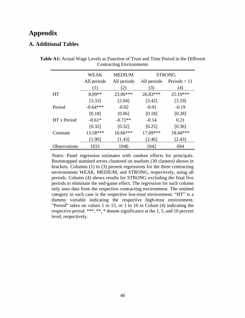
46

Appendix A. Additional Tables

Table A1: Actual Wage Levels as Function of Trust and Time Period in the Different

Contracting Environments

WEAK MEDIUM STRONG All periods All periods All periods Periods < 11 (1) (2) (3) (4) HT 8.09** 23.06*** 26.83*** 25.19*** [3.33] [2.04] [3.42] [3.19] Period -0.64*** -0.02 -0.01 -0.19 [0.18] [0.06] [0.18] [0.28] HT x Period -0.61* -0.71** -0.14 0.21 [0.32] [0.32] [0.25] [0.36] Constant 13.58*** 16.66*** 17.69*** 18.44*** [1.90] [1.43] [2.46] [2.43] Observations 1031 1046 1042 694

Notes: Panel regression estimates with random effects for principals. Bootstrapped standard errors clustered on markets (30 clusters) shown in brackets. Columns (1) to (3) present regressions for the three contracting environments WEAK, MEDIUM, and STRONG, respectively, using all periods. Column (4) shows results for STRONG excluding the final five periods to eliminate the end-game effect. The regression for each column only uses data from the respective contracting environment. The omitted category in each case is the respective low-trust environment. “HT” is a dummy variable indicating the respective high-trust environment. “Period” takes on values 1 to 15, or 1 to 10 in Colum (4) indicating the respective period. ***, **, * denote significance at the 1, 5, and 10 percent level, respectively.

47

Table A2: Effort Levels as Function of Trust and Time Period in the Different Contracting

Environments

WEAK MEDIUM STRONG All periods All periods All periods Periods < 11 (1) (2) (3) (4)

HT 0.76 2.05*** 3.07*** 2.55*** [0.50] [0.50] [0.37] [0.42] Period -0.11*** -0.00 -0.04 0.01 [0.03] [0.02] [0.04] [0.04] HT x Period -0.08** -0.08*** -0.12** -0.01 [0.04] [0.02] [0.05] [0.08] Constant 3.42*** 2.29*** 3.59*** 3.35*** [0.21] [0.30] [0.20] [0.23] Observations 1031 1046 1042 694

Notes: Panel regression estimates with random effects for principals. Bootstrapped standard errors clustered on markets (30 clusters) shown in brackets. Columns (1) to (3) present regressions for the three contracting environments WEAK, MEDIUM, and STRONG, respectively, using all periods. Column (4) shows results for STRONG excluding the final five periods to eliminate the end-game effect. The regression for each column only uses data from the respective contracting environment. The omitted category in each case is the respective low-trust environment. “HT” is a dummy variable indicating the respective high-trust environment. “Period” takes on values 1 to 15, or 1 to 10 in Colum (4) indicating the respective period. ***, **, * denote significance at the 1, 5, and 10 percent level, respectively.

48

Table A3: The Impact of Trust and Contractual Environments on Actual Wages and Effort

Levels

Actual wage Effort All periods Periods < 11 All periods Periods < 11 (1) (2) (3) (4)

HT 17.40*** 17.40*** 1.40*** 1.40*** [3.03] [3.03] [0.44] [0.44] WEAK -8.06*** -8.06*** 0.23 0.23 [1.22] [1.22] [0.24] [0.24] STRONG 1.10 0.94 1.03*** 1.13*** [2.65] [2.67] [0.32] [0.25] HT x WEAK -14.24*** -14.24*** -1.32** -1.32** [3.35] [3.35] [0.52] [0.52] HT x STRONG 8.33* 8.89* 0.75 1.11** [5.02] [4.91] [0.58] [0.55] Constant 16.49*** 16.49*** 2.28*** 2.28*** [0.95] [0.95] [0.19] [0.19] Observations 3119 2771 3119 2771

Notes: Panel regression estimates with random effects for principals. Bootstrapped standard errors clustered on markets (30 clusters) shown in brackets. Columns (1) and (2) present regressions explaining actual wages as a function of contracting and trust environment. The estimations use data from all three contracting environments with LT x MEDIUM as the omitted category. “HT” is a dummy variable indicating the respective high-trust environment. Thus, HT measures the impact of the high-trust environment under medium contract enforcement. WEAK measures the impact of weak contract enforcement relative to MEDIUM in the low-trust environment and STRONG measures the effect of strong contract enforcement relative to MEDIUM in the low-trust environment. HT x WEAK and HT x STRONG give the differential effect of high trust in these respective contracting environments relative to the impact of high trust in MEDIUM. Columns (2) and (4) only use periods 1 to 10 for contracting environment STRONG to eliminate the end-game effect that is present in that environment. In columns (3) and (4) the dependent variable is actual effort levels. ***, **, * denote significance at the 1, 5, and 10 percent level, respectively.

49

Table A4: Relationships of Effort and Profits to Actual Wages in the High Trust Treatments

Effort Profit of principal All periods Periods < 11 All periods Periods < 11 (1) (2) (3) (4)

Actual wage 0.09*** 0.09*** -0.25*** -0.25*** [0.01] [0.01] [0.05] [0.05] WEAK 1.66*** 1.68*** 14.74*** 14.74*** [0.30] [0.30] [2.24] [2.26] STRONG -0.02 0.09 -5.07 -5.21 [0.31] [0.50] [6.55] [8.98] Actual wage x WEAK -0.08*** -0.08*** -0.71*** -0.71*** [0.01] [0.01] [0.11] [0.11] Actual wage x STRONG 0.02** 0.03** 0.33*** 0.42** [0.01] [0.01] [0.13] [0.17] Constant 0.80*** 0.78*** 17.95*** 17.95*** [0.15] [0.16] [1.76] [1.77] Observations 1551 1379 1551 1379

Notes: Panel regression estimates with random effects for principals. Bootstrapped standard errors clustered on markets (15 clusters) shown in brackets. Columns (1) and (2) present regressions explaining effort levels as a function of actual wages and contracting environment. In columns (3) and (4) the dependent variable is profit levels of principals. The estimations use data from the high trust conditions of all three contracting environments with MEDIUM as the omitted category. WEAK is a dummy variable indicating the weak contracting environment, and STRONG indicates the strong contracting environment. “Actual wage” gives the relationship of the dependent variable to actual wages in MEDIUM. Actual wage x WEAK and Actual wage x STRONG give the differential relationship of the dependent variable to higher actual wages in these respective contracting environments relative to the relationship in MEDIUM. The sample excludes outlier wages above 70. Columns (2) and (4) only use periods 1 to 10 for contracting environment STRONG to check robustness to eliminating the end-game effect that is present in that environment. ***, **, * denote significance at the 1, 5, and 10 percent level, respectively.

50

B. Game-Theoretic Analysis The games analyzed in this section are simpler than the games played in the experiment, but they

capture their essential features. We model contracting environment WEAK as a one-shot

simultaneous-move game between a principal, who chooses a wage, and an agent, who chooses a

effort level. We model contracting environment MEDIUM as a one-shot sequential-move game

where the principal first choses the wage, and the agent chooses the effort level after observing

that wage. We model contracting environment STRONG as a simplified dynamic interaction with

two periods, and we capture the excess supply of agents by considering one principal and two

agents. Throughout, we simplify the strategy spaces by assuming that all actions are binary.

Furthermore, the principal is assumed to be profit-maximizing, while the agents can be either

selfish types or reciprocal types. We work with sequential equilibrium as our solution concept. Stage Game Payoffs

The principal chooses a wage 𝑤𝑤 ∈ {𝑤𝑤𝐿𝐿 ,𝑤𝑤𝐻𝐻}, where 0 ≤ 𝑤𝑤𝐿𝐿 < 𝑤𝑤𝐻𝐻. The agent exerts effort 𝑒𝑒 ∈

{𝑒𝑒𝐿𝐿 , 𝑒𝑒𝐻𝐻} where 0 < 𝑒𝑒𝐿𝐿 < 𝑒𝑒𝐻𝐻 < 1, to produce a good of uncertain quality. The good is either

valuable, in which case it generates a payoff of 𝑣𝑣 for the principal, or it is useless and does not

generate any value. Effort 𝑒𝑒 is the probability that the good is valuable. Denote by 𝜔𝜔 ∈ {0,1} the

state of the world describing whether the good is valuable (𝜔𝜔 = 1) or not (𝜔𝜔 = 0). The agent's

cost of providing low effort is normalized to zero; the cost of providing high effort is 𝑐𝑐. Given

actions (𝑤𝑤, 𝑒𝑒), the expected material payoffs of principal and agent are, respectively,

𝜋𝜋𝑃𝑃(𝑤𝑤, 𝑒𝑒) = 𝑒𝑒𝑣𝑣 – 𝑤𝑤 and 𝜋𝜋𝐴𝐴(𝑤𝑤, 𝑒𝑒) = 𝑤𝑤 – �𝑒𝑒 – 𝑒𝑒𝐿𝐿𝑒𝑒𝐻𝐻 – 𝑒𝑒𝐿𝐿

� 𝑐𝑐.

We assume that 0 < 𝑐𝑐 < (𝑒𝑒𝐻𝐻 − 𝑒𝑒𝐿𝐿)𝑣𝑣, which implies that providing the high effort is efficient.

The principal is profit-oriented and maximizes 𝑢𝑢𝑃𝑃(𝑤𝑤, 𝑒𝑒) = 𝜋𝜋𝑃𝑃(𝑤𝑤, 𝑒𝑒). The agent has a type

𝛼𝛼 ∈ {0,𝑎𝑎}, where 0 < 𝑎𝑎 < 1, and maximizes

𝑢𝑢𝐴𝐴(𝑤𝑤, 𝑒𝑒,𝛼𝛼) = 𝜋𝜋𝐴𝐴(𝑤𝑤, 𝑒𝑒) − 𝛼𝛼|𝜋𝜋𝑃𝑃(𝑤𝑤, 𝑒𝑒) − 𝜋𝜋𝐴𝐴(𝑤𝑤, 𝑒𝑒)|.

Type 𝛼𝛼 = 0 is selfish and cares only about own material payoff. Type 𝛼𝛼 = 𝑎𝑎 is inequity-averse,

where the symmetric formulation of inequity-aversion is the simplest way of modelling a

reciprocal motive.26

26 To keep the analysis simple and tractable we use inquity averse preferences to generate reciprocal agent behavior. In principle, one could also model the motive for reciprocal effort

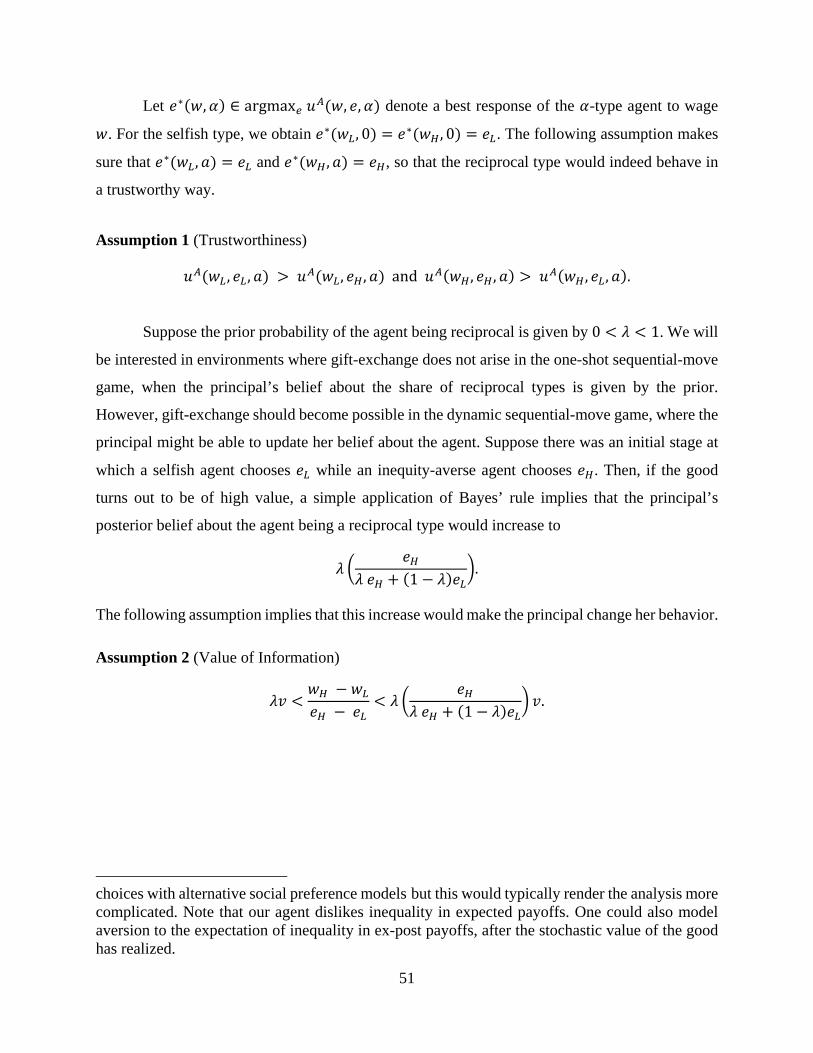
51

Let 𝑒𝑒∗(𝑤𝑤,𝛼𝛼) ∈ argmax𝑒𝑒 𝑢𝑢𝐴𝐴(𝑤𝑤, 𝑒𝑒,𝛼𝛼) denote a best response of the 𝛼𝛼-type agent to wage

𝑤𝑤. For the selfish type, we obtain 𝑒𝑒∗(𝑤𝑤𝐿𝐿 , 0) = 𝑒𝑒∗(𝑤𝑤𝐻𝐻 , 0) = 𝑒𝑒𝐿𝐿. The following assumption makes

sure that 𝑒𝑒∗(𝑤𝑤𝐿𝐿 ,𝑎𝑎) = 𝑒𝑒𝐿𝐿 and 𝑒𝑒∗(𝑤𝑤𝐻𝐻 ,𝑎𝑎) = 𝑒𝑒𝐻𝐻, so that the reciprocal type would indeed behave in

a trustworthy way.

Assumption 1 (Trustworthiness)

𝑢𝑢𝐴𝐴(𝑤𝑤𝐿𝐿 , 𝑒𝑒𝐿𝐿 , 𝑎𝑎) > 𝑢𝑢𝐴𝐴(𝑤𝑤𝐿𝐿 , 𝑒𝑒𝐻𝐻 ,𝑎𝑎) and 𝑢𝑢𝐴𝐴(𝑤𝑤𝐻𝐻 , 𝑒𝑒𝐻𝐻 ,𝑎𝑎) > 𝑢𝑢𝐴𝐴(𝑤𝑤𝐻𝐻 , 𝑒𝑒𝐿𝐿 ,𝑎𝑎).

Suppose the prior probability of the agent being reciprocal is given by 0 < 𝜆𝜆 < 1. We will

be interested in environments where gift-exchange does not arise in the one-shot sequential-move

game, when the principal’s belief about the share of reciprocal types is given by the prior.

However, gift-exchange should become possible in the dynamic sequential-move game, where the

principal might be able to update her belief about the agent. Suppose there was an initial stage at

which a selfish agent chooses 𝑒𝑒𝐿𝐿 while an inequity-averse agent chooses 𝑒𝑒𝐻𝐻. Then, if the good

turns out to be of high value, a simple application of Bayes’ rule implies that the principal’s

posterior belief about the agent being a reciprocal type would increase to

𝜆𝜆 �𝑒𝑒𝐻𝐻

𝜆𝜆 𝑒𝑒𝐻𝐻 + (1 − 𝜆𝜆)𝑒𝑒𝐿𝐿�.

The following assumption implies that this increase would make the principal change her behavior. Assumption 2 (Value of Information)

𝜆𝜆𝑣𝑣 <𝑤𝑤𝐻𝐻 − 𝑤𝑤𝐿𝐿𝑒𝑒𝐻𝐻 − 𝑒𝑒𝐿𝐿

< 𝜆𝜆 �𝑒𝑒𝐻𝐻

𝜆𝜆 𝑒𝑒𝐻𝐻 + (1 − 𝜆𝜆)𝑒𝑒𝐿𝐿� 𝑣𝑣.

choices with alternative social preference models but this would typically render the analysis more complicated. Note that our agent dislikes inequality in expected payoffs. One could also model aversion to the expectation of inequality in ex-post payoffs, after the stochastic value of the good has realized.

52

Contracting Environment WEAK

Suppose the principal and the agent interact only once and choose their actions simultaneously. It

is straightforward to see that this game has a unique equilibrium in which wage and effort are low.

For the principal, paying the low wage is a dominant strategy when choices are simultaneous,

because her wage offer cannot affect the effort chosen by the agent. Both types of the agent then

find it optimal to choose low effort, under Assumption 1. We summarize this in the following

proposition, the formal proof of which is left to the reader.

Proposition 1. Under Assumption 1, the one-shot simultaneous-move game has a

unique sequential equilibrium. In this equilibrium, the principal pays the low wage

and both types of the agent respond with low effort.

Contracting Environment MEDIUM

Now suppose the principal and the agent interact once but choose their actions sequentially. The

wage offered by the principal becomes observable before the agent makes a choice, so that the

principal could affect the effort chosen by the agent. Under Assumption 2, the principal will still

not find it optimal to offer the high wage. This is summarized in the following proposition, the

proof of which is again left to the reader.

Proposition 2. Under Assumptions 1 and 2, the one-shot sequential-move game has a

unique sequential equilibrium. In this equilibrium, the principal pays the low wage

and both types of the agent respond with low effort.

Note, however, that this result depends on the prior belief of the principal about the agent’s

type being pessimistic enough, as embodied by Assumption 2. Suppose an intervention like the

high trustworthiness example in our experiment initially distorts upwards the beliefs of some

principals about the share 𝜆𝜆 of trustworthy types. With sequential moves, we could then expect

some principals to offer high wages initially. It takes some time for them to learn that the high

wage is not reciprocated frequently enough to be profitable, generating a slow learning dynamics

towards the actual equilibrium, in line with our observation in treatment MEDIUM-HT.

53

Contracting Environment STRONG

Now suppose the interaction is repeated and the principal can adjust her contract offer over time.

We consider the following simplified dynamic game between the principal and two agents:

1. The principal chooses wage 𝑤𝑤1.

2. Nature determines agent 1’s type 𝛼𝛼1 (𝛼𝛼1 = 𝑎𝑎 with independent probability 𝜆𝜆).

3. Agent 1 chooses effort 𝑒𝑒1.

4. Nature determines the state 𝜔𝜔1 (𝜔𝜔1 = 1 with independent probability 𝑒𝑒1).

5. The principal chooses whether to keep agent 1 (𝑘𝑘 = 1) or to fire her and hire agent 2 instead

(𝑘𝑘 = 0). The principal also chooses wage 𝑤𝑤2 for the second period.

6. Nature determines agent 2’s type 𝛼𝛼2 (𝛼𝛼2 = 𝑎𝑎 with independent probability 𝜆𝜆).

7. The hired agent chooses effort 𝑒𝑒2.

8. Nature determines the state 𝜔𝜔2 (𝜔𝜔2 = 1 with independent probability 𝑒𝑒2).

For notational simplicity, we assume that nature determines agent 2’s type 𝛼𝛼2 even if the

agent is not hired in the second period. The terminal nodes of the dynamic game are then given by

𝑡𝑡 = (𝑤𝑤1,𝛼𝛼1, 𝑒𝑒1,𝜔𝜔1,𝑘𝑘,𝑤𝑤2,𝛼𝛼2, 𝑒𝑒2,𝜔𝜔2). The players’ payoffs are

𝑈𝑈𝑃𝑃(𝑡𝑡) = 𝑢𝑢𝑃𝑃(𝑤𝑤1,𝜔𝜔1) + 𝑢𝑢𝑃𝑃(𝑤𝑤2,𝜔𝜔2),

𝑈𝑈1𝐴𝐴(𝑡𝑡) = 𝑢𝑢𝐴𝐴(𝑤𝑤1, 𝑒𝑒1,𝛼𝛼1) + 𝑘𝑘𝑢𝑢𝐴𝐴(𝑤𝑤2, 𝑒𝑒2,𝛼𝛼1),

𝑈𝑈2𝐴𝐴(𝑡𝑡) = (1 − 𝑘𝑘)𝑢𝑢𝐴𝐴(𝑤𝑤2, 𝑒𝑒2,𝛼𝛼2).

Note that we assume here that the inequity-averse agents compare themselves only with the

principal, separately period by period, whenever they interact.

Concerning the information structure, we assume that an agent’s type and effort choice is

observable only to the agent herself, while everything else is observable to all players.27 A (pure)

strategy of the principal prescribes the wage to be chosen in the root of the game, 𝑠𝑠𝑃𝑃(∅) ∈

{𝑤𝑤𝐿𝐿 ,𝑤𝑤𝐻𝐻}, as well as for each observed history (𝑤𝑤1,𝜔𝜔1) a hiring decision and the wage offered in

the second period, 𝑠𝑠𝑃𝑃(𝑤𝑤1,𝜔𝜔1) ∈ {0,1} × {𝑤𝑤𝐿𝐿 ,𝑤𝑤𝐻𝐻}. A strategy of agent 1 prescribes an effort to be

chosen in the first period for each observed wage-type combination, 𝑠𝑠1𝐴𝐴(𝑤𝑤1 ,𝛼𝛼1) ∈ {𝑒𝑒𝐿𝐿 , 𝑒𝑒𝐻𝐻}, and

27 We could also assume that wage offers are only observable to the currently hired agent, and/or that the realized value of the good is observable only to the principal. This would complicate the notation of beliefs, but we would still obtain the equilibrium outcomes derived below.

54

an effort to be chosen conditional on all observables in case she is hired again in the second period,

𝑠𝑠1𝐴𝐴(𝑤𝑤1,𝛼𝛼1, 𝑒𝑒1,𝜔𝜔1, 1,𝑤𝑤2) ∈ {𝑒𝑒𝐿𝐿 , 𝑒𝑒𝐻𝐻}. Finally, a strategy of agent 2 prescribes a effort to be chosen

conditional on all observables in case she is hired in the second period, 𝑠𝑠2𝐴𝐴(𝑤𝑤1,𝜔𝜔1, 0,𝑤𝑤2,𝛼𝛼2) ∈

{𝑒𝑒𝐿𝐿 , 𝑒𝑒𝐻𝐻}. For each of the observable histories at which a player acts, she maintains a probabilistic

belief over the nodes in the corresponding information set, i.e., a belief about the earlier

unobservable actions that led to this information set.

In a first step, we describe conditions under which the game admits a sequential equilibrium

that replicates the one-shot equilibrium outcome: The principal initially pays the low wage and

both types of the first agent respond with low effort; the principal then always fires the first agent

and offers the low wage to the second agent, who responds with low effort. We refer to such an

equilibrium as a low-trust equilibrium. It can exist if the principal correctly believes that a high

wage would not elicit high effort from any type of the first agent, and hence would also not

facilitate learning about that agent’s type. It will turn out that the binding constraint for this

construction is the reciprocal first agent’s incentive not to respond to a high wage with high effort.

The following assumption makes sure that this constraint can be satisfied. Assumption 3 (Low-Trust Incentive-Compatibility)

(𝑒𝑒𝐻𝐻 − 𝑒𝑒𝐿𝐿)𝑢𝑢𝐴𝐴(𝑤𝑤𝐿𝐿 , 𝑒𝑒𝐿𝐿 ,𝑎𝑎) > 𝑢𝑢𝐴𝐴(𝑤𝑤𝐻𝐻 , 𝑒𝑒𝐻𝐻 ,𝑎𝑎) − 𝑢𝑢𝐴𝐴(𝑤𝑤𝐻𝐻 , 𝑒𝑒𝐿𝐿 ,𝑎𝑎).

We can now state the following result.

Proposition 3. Under Assumptions 1, 2, and 3 the dynamic game has a low-trust

sequential equilibrium.

Proof: We first characterize agent 2’s strategy in any sequential equilibrium. After observing any

history (𝑤𝑤1,𝜔𝜔1, 0,𝑤𝑤2,𝛼𝛼2) she entertains a belief about (𝛼𝛼1, 𝑒𝑒1), which must be consistent with the

requirements imposed by sequential equilibrium. However, her optimal behavior does not depend

on these beliefs. Under Assumption 1, we always obtain the unique sequentially rational choice

𝑠𝑠2𝐴𝐴(𝑤𝑤1,𝜔𝜔1, 0,𝑤𝑤2,𝛼𝛼2) = 𝑒𝑒∗(𝑤𝑤2,𝛼𝛼2). We next characterize agent 1’s second-period strategy in any

sequential equilibrium. After observing any history (𝑤𝑤1,𝛼𝛼1, 𝑒𝑒1,𝜔𝜔1, 1,𝑤𝑤2) she entertains a belief

about 𝛼𝛼2, which must be consistent with the requirements imposed by sequential equilibrium.

55

However, her optimal behavior does not depend on these beliefs. Under Assumption 1, we obtain

the unique sequentially rational choice 𝑠𝑠1𝐴𝐴(𝑤𝑤1,𝛼𝛼1, 𝑒𝑒1,𝜔𝜔1, 1,𝑤𝑤2) = 𝑒𝑒∗(𝑤𝑤2,𝛼𝛼1).

We now subsume these choices directly into the players’ payoff functions and treat the game

as a reduced game between the principal and agent 1. It ends in the terminal nodes �̂�𝑡 =

(𝑤𝑤1,𝛼𝛼1, 𝑒𝑒1,𝜔𝜔1,𝑘𝑘,𝑤𝑤2) with payoffs

𝑈𝑈𝑃𝑃(�̂�𝑡) = 𝑢𝑢𝑃𝑃(𝑤𝑤1,𝜔𝜔1) + 𝑘𝑘𝑢𝑢𝑃𝑃�𝑤𝑤2, 𝑒𝑒∗(𝑤𝑤2,𝛼𝛼1)�

+(1 − 𝑘𝑘)�𝜆𝜆𝑢𝑢𝑃𝑃�𝑤𝑤2, 𝑒𝑒∗(𝑤𝑤2,𝑎𝑎)� + (1 − 𝜆𝜆)𝑢𝑢𝑃𝑃�𝑤𝑤2, 𝑒𝑒∗(𝑤𝑤2, 0)��,

𝑈𝑈1𝐴𝐴(�̂�𝑡) = 𝑢𝑢𝐴𝐴(𝑤𝑤1, 𝑒𝑒1,𝛼𝛼1) + 𝑘𝑘𝑢𝑢𝐴𝐴(𝑤𝑤2, 𝑒𝑒∗(𝑤𝑤2,𝛼𝛼1),𝛼𝛼1).

This reduced game has two proper subgames, one starting after each possible first period wage

offer. In each of these subgames, the only non-singleton information sets are those of the principal

when observing (𝑤𝑤1,𝜔𝜔1), where she entertains beliefs about (𝛼𝛼1, 𝑒𝑒1). Since 𝑒𝑒𝐿𝐿 > 0 and 𝑒𝑒𝐻𝐻 < 1,

these beliefs can always be determined by Bayes' rule when we start from the root of the respective

subgame. This uniquely pins down the consistent beliefs in any sequential equilibrium.

Consider first the subgame starting after 𝑤𝑤1 = 𝑤𝑤𝐿𝐿. Let the strategies in this subgame be

given by

𝑠𝑠1𝐴𝐴(𝑤𝑤𝐿𝐿 , 0) = 𝑠𝑠1𝐴𝐴(𝑤𝑤𝐿𝐿 ,𝑎𝑎) = 𝑒𝑒𝐿𝐿 and 𝑠𝑠𝑃𝑃(𝑤𝑤𝐿𝐿 , 0) = 𝑠𝑠𝑃𝑃(𝑤𝑤𝐿𝐿 , 1) = (0,𝑤𝑤𝐿𝐿),

i.e., both types of the first agent respond with low effort, and, irrespective of the realized value of

the good, the principal then hires the second agent and pays the low wage. Given any observation

of (𝑤𝑤𝐿𝐿 ,𝜔𝜔1), the principal entertains a probabilistic belief about (𝛼𝛼1, 𝑒𝑒1), but only the marginal

distribution of 𝛼𝛼1 matters for her sequentially rational choices (since 𝑒𝑒1 is not payoff relevant

conditional on 𝜔𝜔1, and later behavior also does not depend on 𝑒𝑒1). Denoting the probability

attached to 𝛼𝛼1 = 𝑎𝑎 by 𝛽𝛽𝑃𝑃(𝑤𝑤𝐿𝐿 ,𝜔𝜔1), we obtain 𝛽𝛽𝑃𝑃(𝑤𝑤𝐿𝐿 , 0) = 𝛽𝛽𝑃𝑃(𝑤𝑤𝐿𝐿 , 1) = 𝜆𝜆 from Bayes’ rule. It

then follows immediately from Assumptions 1 and 2 that the principal’s strategy is indeed

sequentially rational. As for the agent, observe that deviations cannot affect the principal’s second

period behavior. It then follows from Assumption 1 that the agent’s strategy is also sequentially

rational. The resulting expected payoff of the principal in the root of this subgame is 𝑈𝑈𝐿𝐿𝑃𝑃 =

2𝑢𝑢𝑃𝑃(𝑤𝑤𝐿𝐿 , 𝑒𝑒𝐿𝐿).

Consider now the subgame starting after 𝑤𝑤1 = 𝑤𝑤𝐻𝐻. Let the strategies in this subgame be

given by

56

𝑠𝑠1𝐴𝐴(𝑤𝑤𝐻𝐻 , 0) = 𝑠𝑠1𝐴𝐴(𝑤𝑤𝐻𝐻 ,𝑎𝑎) = 𝑒𝑒𝐿𝐿 and 𝑠𝑠𝑃𝑃(𝑤𝑤𝐻𝐻 , 0) = (1,𝑤𝑤𝐿𝐿), 𝑠𝑠𝑃𝑃(𝑤𝑤𝐻𝐻 , 1) = (0,𝑤𝑤𝐿𝐿),

i.e., both types of the first agent respond with low effort and the principal always pays the low

wage in the second period, keeping the first agent if and only if the good is of low value. We obtain

the beliefs 𝛽𝛽𝑃𝑃(𝑤𝑤𝐻𝐻 , 0) = 𝛽𝛽𝑃𝑃(𝑤𝑤𝐻𝐻 , 1) = 𝜆𝜆. Under Assumptions 1 and 2, the principal thus wants to

pay the low wage in the second period and is indifferent between keeping and firing the agent,

which makes her strategy sequentially rational. As for the agent, consider type 𝛼𝛼1 = 0 first.

Assumption 1 implies that 𝑒𝑒𝐿𝐿 maximizes her first-period payoff. Moreover,

𝑢𝑢𝐴𝐴(𝑤𝑤𝐿𝐿 , 𝑒𝑒∗(𝑤𝑤𝐿𝐿 , 0), 0) = 𝑤𝑤𝐿𝐿 ≥ 0 implies that the selfish agent (weakly) benefits from a larger

probability of being hired again in the second period, which implies that her strategy is sequentially

rational. Consider next type 𝛼𝛼1 = 𝑎𝑎, who faces a trade-off between her payoff-maximizing

response in the first period and the probability of being hired again in the second period. The

condition for 𝑠𝑠1𝐴𝐴(𝑤𝑤𝐻𝐻 ,𝑎𝑎) = 𝑒𝑒𝐿𝐿 to be sequentially rational is

𝑢𝑢𝐴𝐴(𝑤𝑤𝐻𝐻 , 𝑒𝑒𝐿𝐿 , 𝑎𝑎) + (1 − 𝑒𝑒𝐿𝐿)𝑢𝑢𝐴𝐴(𝑤𝑤𝐿𝐿 , 𝑒𝑒∗(𝑤𝑤𝐿𝐿 ,𝑎𝑎),𝑎𝑎)

≥ 𝑢𝑢𝐴𝐴(𝑤𝑤𝐻𝐻 , 𝑒𝑒𝐻𝐻 ,𝑎𝑎) + (1 − 𝑒𝑒𝐻𝐻)𝑢𝑢𝐴𝐴(𝑤𝑤𝐿𝐿 , 𝑒𝑒∗(𝑤𝑤𝐿𝐿 ,𝑎𝑎),𝑎𝑎),

which is satisfied under Assumptions 1 and 3. The resulting expected payoff of the principal in the

root of this subgame is 𝑈𝑈𝐻𝐻𝑃𝑃 = 𝑢𝑢𝑃𝑃(𝑤𝑤𝐻𝐻 , 𝑒𝑒𝐿𝐿) + 𝑢𝑢𝑃𝑃(𝑤𝑤𝐿𝐿 , 𝑒𝑒𝐿𝐿).

Given the strategies and payoffs in the two subgames, it follows that 𝑠𝑠𝑃𝑃(∅) = 𝑤𝑤𝐿𝐿 is the

sequentially rational first-period wage for the principal. ∎ Next, we describe conditions under which the game admits an equilibrium in which gift-

exchange occurs. The principal initially pays the high wage, to which a selfish agent responds with

low effort and a reciprocal agent responds with high effort. The principal then always keeps the

agent but offers the high wage in the second period if and only if the good turns out to be valuable.

Thus, the principal tries to screen the reciprocal types from the selfish types. We refer to such an

equilibrium as a high-trust equilibrium. Several constraints have to be satisfied for this equilibrium

to exist, which we summarize in the following.

57

Assumption 4 (High-Trust Incentive-Compatibility)

(𝑖𝑖) 𝑢𝑢𝐴𝐴(𝑤𝑤𝐻𝐻 , 𝑒𝑒𝐿𝐿 , 0) − 𝑢𝑢𝐴𝐴(𝑤𝑤𝐻𝐻 , 𝑒𝑒𝐻𝐻 , 0) > (𝑒𝑒𝐻𝐻 − 𝑒𝑒𝐿𝐿)[𝑢𝑢𝐴𝐴(𝑤𝑤𝐻𝐻 , 𝑒𝑒𝐿𝐿 , 0) − 𝑢𝑢𝐴𝐴(𝑤𝑤𝐿𝐿 , 𝑒𝑒𝐿𝐿 , 0)],

(𝑖𝑖𝑖𝑖) 𝑢𝑢𝐴𝐴(𝑤𝑤𝐻𝐻 , 𝑒𝑒𝐻𝐻 ,𝑎𝑎) − 𝑢𝑢𝐴𝐴(𝑤𝑤𝐻𝐻 , 𝑒𝑒𝐿𝐿 , 𝑎𝑎) > (𝑒𝑒𝐻𝐻 − 𝑒𝑒𝐿𝐿)[𝑢𝑢𝐴𝐴(𝑤𝑤𝐿𝐿 , 𝑒𝑒𝐿𝐿 ,𝑎𝑎) − 𝑢𝑢𝐴𝐴(𝑤𝑤𝐻𝐻 , 𝑒𝑒𝐻𝐻 ,𝑎𝑎)],

(𝑖𝑖𝑖𝑖𝑖𝑖) 𝑢𝑢𝑃𝑃(𝑤𝑤𝐻𝐻 , 𝜆𝜆𝑒𝑒𝐻𝐻 + (1 − 𝜆𝜆)𝑒𝑒𝐿𝐿) + 𝜆𝜆𝑒𝑒𝐻𝐻𝑢𝑢𝑃𝑃(𝑤𝑤𝐻𝐻 , 𝑒𝑒𝐻𝐻) + (1 − 𝜆𝜆)𝑒𝑒𝐿𝐿𝑢𝑢𝑃𝑃(𝑤𝑤𝐻𝐻 , 𝑒𝑒𝐿𝐿)

> [2 − 𝜆𝜆(1 − 𝑒𝑒𝐻𝐻) − (1 − 𝜆𝜆)(1 − 𝑒𝑒𝐿𝐿)] 𝑢𝑢𝑃𝑃(𝑤𝑤𝐿𝐿 , 𝑒𝑒𝐿𝐿).

We can now state the following result. Proposition 4: Under Assumptions 1, 2, and 4, the dynamic game has a high-trust

sequential equilibrium.

Proof: Consider again the reduced game between the principal and agent 1 constructed in the proof

of Proposition 3. Also, let the strategies and beliefs in the subgame starting after 𝑤𝑤1 = 𝑤𝑤𝐿𝐿 be the

same as in the proof of Proposition 3, i.e.,

𝑠𝑠1𝐴𝐴(𝑤𝑤𝐿𝐿 , 0) = 𝑠𝑠1𝐴𝐴(𝑤𝑤𝐿𝐿 ,𝑎𝑎) = 𝑒𝑒𝐿𝐿 and 𝑠𝑠𝑃𝑃(𝑤𝑤𝐿𝐿 , 0) = 𝑠𝑠𝑃𝑃(𝑤𝑤𝐿𝐿 , 1) = (0,𝑤𝑤𝐿𝐿),

where 𝛽𝛽𝑃𝑃(𝑤𝑤𝐿𝐿 , 0) = 𝛽𝛽𝑃𝑃(𝑤𝑤𝐿𝐿 , 1) = 𝜆𝜆, with a resulting expected payoff for the principal in the root

of this subgame of 𝑈𝑈𝐿𝐿𝑃𝑃 = 2𝑢𝑢𝑃𝑃(𝑤𝑤𝐿𝐿 , 𝑒𝑒𝐿𝐿).

Consider now the subgame starting after 𝑤𝑤1 = 𝑤𝑤𝐻𝐻. Let the strategies be given by

𝑠𝑠1𝐴𝐴(𝑤𝑤𝐻𝐻 , 0) = 𝑒𝑒𝐿𝐿 , 𝑠𝑠1𝐴𝐴(𝑤𝑤𝐻𝐻 ,𝑎𝑎) = 𝑒𝑒𝐻𝐻 and 𝑠𝑠𝑃𝑃(𝑤𝑤𝐻𝐻 , 0) = (1,𝑤𝑤𝐿𝐿), 𝑠𝑠𝑃𝑃(𝑤𝑤𝐻𝐻 , 1) = (1,𝑤𝑤𝐻𝐻),

i.e., the selfish agent responds with low effort and the trustworthy agent responds with high effort,

while the principal always keeps the agent but pays the high wage in the second period only if the

good turns out to be valuable. Given these strategies, an application of Bayes’ rule yields the

following consistent beliefs:

𝛽𝛽𝑃𝑃(𝑤𝑤𝐻𝐻 , 0) =𝜆𝜆 (1 − 𝑒𝑒𝐻𝐻)

𝜆𝜆 (1 − 𝑒𝑒𝐻𝐻) + (1 − 𝜆𝜆)(1 − 𝑒𝑒𝐿𝐿) < 𝜆𝜆,

𝛽𝛽𝑃𝑃(𝑤𝑤𝐻𝐻 , 1) =𝜆𝜆𝑒𝑒𝐻𝐻

𝜆𝜆𝑒𝑒𝐻𝐻 + (1 − 𝜆𝜆)𝑒𝑒𝐿𝐿> 𝜆𝜆.

Assumptions 1 and 2 now immediately imply that the principal’s strategy is sequentially

rational. As for the agent, consider type 𝛼𝛼1 = 0 first. The condition for 𝑠𝑠1𝐴𝐴(𝑤𝑤𝐻𝐻 , 0) = 𝑒𝑒𝐿𝐿 to be

sequentially rational is

58

𝑢𝑢𝐴𝐴(𝑤𝑤𝐻𝐻 , 𝑒𝑒𝐿𝐿 , 0) + 𝑒𝑒𝐿𝐿𝑢𝑢𝐴𝐴(𝑤𝑤𝐻𝐻 , 𝑒𝑒∗(𝑤𝑤𝐻𝐻 , 0), 0) + (1 − 𝑒𝑒𝐿𝐿)𝑢𝑢𝐴𝐴(𝑤𝑤𝐿𝐿 , 𝑒𝑒∗(𝑤𝑤𝐿𝐿 , 0), 0)

≥ 𝑢𝑢𝐴𝐴(𝑤𝑤𝐻𝐻 , 𝑒𝑒𝐻𝐻 , 0) + 𝑒𝑒𝐻𝐻𝑢𝑢𝐴𝐴(𝑤𝑤𝐻𝐻 , 𝑒𝑒∗(𝑤𝑤𝐻𝐻 , 0),0) + (1 − 𝑒𝑒𝐻𝐻)𝑢𝑢𝐴𝐴(𝑤𝑤𝐿𝐿 , 𝑒𝑒∗(𝑤𝑤𝐿𝐿 , 0),0),

which is satisfied under Assumptions 1 and 4(i). Now consider type 𝛼𝛼1 = 𝑎𝑎. The condition for

𝑠𝑠1𝐴𝐴(𝑤𝑤𝐻𝐻 ,𝑎𝑎) = 𝑒𝑒𝐻𝐻 to be sequentially rational is

𝑢𝑢𝐴𝐴(𝑤𝑤𝐻𝐻 , 𝑒𝑒𝐻𝐻 ,𝑎𝑎) + 𝑒𝑒𝐻𝐻𝑢𝑢𝐴𝐴(𝑤𝑤𝐻𝐻 , 𝑒𝑒∗(𝑤𝑤𝐻𝐻 ,𝑎𝑎),𝑎𝑎) + (1 − 𝑒𝑒𝐻𝐻)𝑢𝑢𝐴𝐴(𝑤𝑤𝐿𝐿 , 𝑒𝑒∗(𝑤𝑤𝐿𝐿 ,𝑎𝑎),𝑎𝑎)

≥ 𝑢𝑢𝐴𝐴(𝑤𝑤𝐻𝐻 , 𝑒𝑒𝐿𝐿 ,𝑎𝑎) + 𝑒𝑒𝐿𝐿𝑢𝑢𝐴𝐴(𝑤𝑤𝐻𝐻 , 𝑒𝑒∗(𝑤𝑤𝐻𝐻 ,𝑎𝑎),𝑎𝑎) + (1 − 𝑒𝑒𝐿𝐿)𝑢𝑢𝐴𝐴(𝑤𝑤𝐿𝐿 , 𝑒𝑒∗(𝑤𝑤𝐿𝐿 ,𝑎𝑎),𝑎𝑎),

which is satisfied under Assumptions 1 and 4(ii). The resulting expected payoff of the principal in

the root of this subgame is

𝑈𝑈𝐻𝐻𝑃𝑃 = 𝜆𝜆𝑒𝑒𝐻𝐻[𝑢𝑢𝑃𝑃(𝑤𝑤𝐻𝐻 , 1) + 𝑢𝑢𝑃𝑃(𝑤𝑤𝐻𝐻 , 𝑒𝑒𝐻𝐻)]

+𝜆𝜆(1 − 𝑒𝑒𝐻𝐻)[𝑢𝑢𝑃𝑃(𝑤𝑤𝐻𝐻 , 0) + 𝑢𝑢𝑃𝑃(𝑤𝑤𝐿𝐿 , 𝑒𝑒𝐿𝐿)]

+(1 − 𝜆𝜆)𝑒𝑒𝐿𝐿[𝑢𝑢𝑃𝑃(𝑤𝑤𝐻𝐻 , 1) + 𝑢𝑢𝑃𝑃(𝑤𝑤𝐻𝐻 , 𝑒𝑒𝐿𝐿)]

+(1 − 𝜆𝜆)(1 − 𝑒𝑒𝐿𝐿)[𝑢𝑢𝑃𝑃(𝑤𝑤𝐻𝐻 , 0) + 𝑢𝑢𝑃𝑃(𝑤𝑤𝐿𝐿 , 𝑒𝑒𝐿𝐿)].

Now consider the principal’s choice of the first-period wage. The condition 𝑈𝑈𝐻𝐻𝑃𝑃 ≥ 𝑈𝑈𝐿𝐿𝑃𝑃 is

satisfied under Assumption 4(iii), which implies that 𝑠𝑠𝑃𝑃(∅) = 𝑤𝑤𝐻𝐻 is sequentially rational for the

principal. ∎

It remains to be shown that Assumptions 1 – 4 can be satisfied simultaneously, so that the

low-trust and the high-trust equilibrium coexist. In fact, it can be shown that they are jointly

satisfied by a large range of values of the underlying parameters, including values that resemble

the payoff structure in the experiment. For instance, let 𝑣𝑣 = 100, 𝑐𝑐 = 15, 𝑤𝑤𝐿𝐿 = 20, 𝑤𝑤𝐻𝐻 = 40,

𝑒𝑒𝐿𝐿 = 1/3 and 𝑒𝑒𝐻𝐻 = 2/3. Also choose 𝑎𝑎 = 0.4 and 𝜆𝜆 = 0.55. It is easy to show that all assumptions

are satisfied by these parameters. It holds that all players’ expected payoffs are non-negative in

equilibrium (even in each period separately), so that participation constraints would also be

satisfied.

We interpret the historical examples about agent trustworthiness in our experiment as an

equilibrium selection device, so that the high-trust equilibrium corresponds to treatment

STRONG-HT and the low-trust equilibrium corresponds to treatment STRONG-LT.

Consider the low-trust equilibrium first. The offered wage and the returned effort are always

low on the equilibrium path, in both periods. If the principal actually trembled and mistakenly

59

offered the high wage in the first period, both agent types would still respond with low effort. The

off-equilibrium behavior thus confirms the pattern shown in the low trustworthiness example.

Now consider the high-trust equilibrium. On the equilibrium path, the first-period wage is

always high, 𝑤𝑤𝐻𝐻, while the average second-period wage (across many independent repetitions of

the game) is given by

[𝜆𝜆𝑒𝑒𝐻𝐻 + (1 − 𝜆𝜆)𝑒𝑒𝐿𝐿] 𝑤𝑤𝐻𝐻 + [𝜆𝜆(1 − 𝑒𝑒𝐻𝐻) + (1 − 𝜆𝜆)(1 − 𝑒𝑒𝐿𝐿)]𝑤𝑤𝐿𝐿 ,

reflecting that the principal offers the high wage only if the first-period good turns out to be

valuable. Hence, we predict some endgame effect in wages. As for effort, the average first-period

effort is 𝜆𝜆𝑒𝑒𝐻𝐻 + (1 − 𝜆𝜆)𝑒𝑒𝐿𝐿 in equilibrium. The average second-period effort is (𝜆𝜆𝑒𝑒𝐻𝐻)𝑒𝑒𝐻𝐻 +

(1 − 𝜆𝜆𝑒𝑒𝐻𝐻)𝑒𝑒𝐿𝐿, reflecting that only trustworthy agents who produced a good of high value are

induced to provide the high effort again in the second period. Hence, there should also be some

endgame effect in effort. Notice that a response of effort to wage can be observed on the

equilibrium path in the high-trust equilibrium. The high wage is associated with an average effort

of 𝜆𝜆𝑒𝑒𝐻𝐻 + (1 − 𝜆𝜆)𝑒𝑒𝐿𝐿 in the first period and with an even larger average effort of �̅�𝛽𝑒𝑒𝐻𝐻 + �1 − �̅�𝛽�𝑒𝑒𝐿𝐿

in the second period, where

�̅�𝛽 = 𝜆𝜆 �𝑒𝑒𝐻𝐻

𝜆𝜆 𝑒𝑒𝐻𝐻 + (1 − 𝜆𝜆)𝑒𝑒𝐿𝐿�.

By contrast, the low wage in the second period is always associated with the low effort. Similarly,

if the principal trembled and offered the low wage in the first period, both agent types would

respond with low effort. This confirms the responsive pattern where agents choose higher average

effort when wages are higher, as shown in the high trustworthiness example.

60

C. Experimental Instructions In this appendix, we provide an English translation of the original German of treatment pair

STONG-HT and STRONG-LT and of treatment pair MEDIUM-HT and MEDIUM-LT.

Comments in square brackets indicate where the instructions differ between the treatments. The

instructions for the treatment pair WEAK-HT and WEAK-LT are identical to the respective

instructions for MEDIUM-HT and MEDIUM-LT, except that they specify that (i) buyers are not

obliged to pay the offered wage and (ii) actual wages and effort levels are chosen simultaneously.

The instructions for treatment STONG-HT-Long are identical to the instruction for treatment

STRONG-HT, except that they specify that the game lasts for 25 periods and a slightly different

exchange rate between points to account for the fact that subjects were paid for 10 additional

periods. The original German instructions for all treatments are available from the authors upon

request.

61

C1. Buyer Instructions

Instructions for buyers

You are now participating in an economic study. Please read the following instructions carefully. Here you will learn everything you need to know to participate in the study. Please raise your hand if you do not understand something. We will answer your question at your desk. You will receive an initial endowment of 20 Swiss francs at the beginning of the study. You can earn additional income during the study by earning points. The number of points you earn during the study depends on your choices and on those of the other participants. All the points you earn during the course of the study will be converted to Swiss francs at the end of the study. The following conversion rate applies:

10 points = 1 Swiss franc You will receive the monetary amount you earned during the study plus the 20 Swiss francs initial endowment in cash at the end of the study. The study is divided into individual periods. You must make decisions each period which you enter into the computer. There are a total of 15 periods. Please note that communication is strictly forbidden during the study. Furthermore, we inform you that you may only use those functions on the computer that are necessary for completing the study. Communication or playing with the computer lead to exclusion from the study. We remain at your disposal to answer any questions you might have. The 34 participants were divided into two completely independent groups of 17 participants each before the beginning of the study. You will only interact within your group of 17 participants during the study. The participants in each group of 17 are then divided into 10 sellers and 7 buyers each. You are a buyer during the entire study. [Treatments STRONG-HT/ STRONG-LT:] All participants have an identification number that they retain for the entire duration of the study. Your identification number is on the documentation sheet in front of you. [Treatments MEDIUM-HT/MEDIUM-LT:] All participants have an identification number that changes randomly in each period. [Identical instructions from here onwards.]

62

Short summary of the procedure of the study Each buyer can trade a product with a seller in each period of the study. The seller realizes a profit if he/she obtains a sales wage that exceeds his/her production costs. The production costs depend on the effort of the product. The higher the effort of the product that the seller chooses, the higher are his/her production costs. The buyer realizes a profit if he/she pays less for the product than its value to him/her. The value of a product is either 100 points (the product is exceptionally good) or 10 points (the product just fulfills its objective). The higher the effort that the seller selects, the higher the probability that the value of the product for the buyer is 100 points. The study lasts a total of 15 periods. The procedure in an individual period is organized as follows: 1. Each period begins with a negotiation phase that lasts for three minutes. Buyers can make

purchase offers that sellers can accept during this time.

When making a purchase offer, a buyer must determine three things:

• the wage he/she offers; • the effort he/she desires; • and finally to which seller he/she is directing the purchase offer. Buyers can make two

types of purchase offers: private and public. Private purchase offers are only directed to one seller and can only be accepted by this seller. Public purchase offers are directed to all sellers and can thus be accepted by any seller.

As a buyer, you can make as many purchase offers as you want in each period. An offer which is made can be accepted at any time. Each seller and each buyer can only conclude a maximum of one trade in each period. As there are a total of ten sellers and seven buyers, some sellers will not be able to participate in each period.

2. After the negotiation phase, all sellers who have concluded a trade must determine the product

effort that they want to deliver to their buyer. The seller must not respect the buyer's requested effort. After all of the sellers have selected their product effort, it will be determined whether the value for each buyer is 100 points or 10 points. The higher the seller's selected effort, the higher the probability that the value for the buyer is 100 points. Once these values have been determined, the earnings for this period are settled for this period. Then the next period begins.

The income from all 15 periods will be added together at the end of the study, converted to Swiss francs, and paid out together with the initial endowment in cash.

63

Detailed procedure of the study There are 7 buyers and 10 sellers in your group of 17. You are a buyer for the entire study. You will enter your decisions on the computer during the study. The information below shows you in detail how you make your decisions in each period. 1. The negotiation phase Each period of the study begins with a negotiation phase. Each buyer can conclude a trade with one seller in the negotiation phase. Each buyer can make as many purchase offers as he/she wants to during this phase. You will see the following decision screen during each negotiation phase:

[Text on screen: Period 1 of 15 / remaining time / public purchase offers buyer wage requested effort / your private offers wage requested effort to seller / your identification number / you make your offers here / public / private / if private, to which seller? / your wage / requested effort / OK / your seller / your wage / your requested effort] • You see which period you are in at the upper left corner of the screen. The remaining time in

this negotiation phase appears at the upper right corner. The negotiation phase lasts three minutes (=180 seconds) in each negotiation phase. Once the time has expired, the negotiation phase is over. Further purchase offers may neither be made nor accepted in this period.

5

64

[Only treatments MEDIUM-HT/MEDIUM-LT, but not STRONG-HT/STRONG-LT, include the following bullet point:] • The next item you see is your identification number. This identification number is randomly

redetermined in each period. This applies to all study participants, i.e. for all sellers and for all buyers.

• As soon as you see the screen above, the negotiation phase is opened. You as a buyer now have the opportunity to make purchase offers to the sellers. To do this you must determine three things on the right side of the screen:

a) You first must determine if you want to make a public or private purchase offer:

• Public purchase offers Public purchase offers are notified to all participants in the market. All sellers see all public

purchase offers on their screens. Each seller can thus accept a public purchase offer. You as buyer also see all public purchase offers from the other buyers. If you want to make a public purchase offer, click on the field "public" with your mouse.

• Private purchase offers

Private purchase offers are only directed towards one seller. Only this seller learns of the offer, and only this seller may accept the purchase offer. No other sellers and buyers in the market will learn about this offer. If you want to make a private purchase offer, click on the field "private" with the mouse. Then indicate in the field below to which seller you direct the purchase offer. All ten sellers have an identification number (seller 1, seller 2, …, seller 10). [Treatments STRONG-HT/STRONG-LT:] The sellers retain this number for the duration of the study. [Treatments HT-R/LT-R:] This identification number varies randomly in each period of the study. [Identical instructions from here onwards.] To direct an offer to a specific seller, enter the seller's number (e.g. "4" for seller 4).

b) After you have determined to whom you want to direct your purchase offer, you must

determine your purchase offer. Enter this in the field "your wage". The purchase offer may neither be less than 0 nor greater than 100.

0 ≤ purchase offer ≤ 100

c) Finally, you must then enter the product effort you desire. Enter this in the field

"requested effort". The requested product effort may neither be less than 1 nor higher than 9:

1 ≤ requested product effort ≤ 9

• After you have completely determined your purchase offer, you must click on the "OK" button

to publicize the offer. You may revise your offer until you click the "OK" button. After you click on the "OK" button, your purchase offer will appear to all sellers to whom it was directed.

65

• You see the heading "public offers" on the left side of your screen. All public offers in the current negotiation phase appear here. Both your own offers as well as the public offers from the other buyers appear here. You can see which buyer made the offer, the wage he/she offers, and the effort he/she desires. [Treatments STRONG-HT/STRONG-LT:] All buyers also have an identification number in the study that applies for the entire duration of the study (buyer 1, buyer 2, … buyer 7). [Treatments MEDIUM-HT/MEDIUM-LT:] All buyers in the study also have an identification number between one and seven in each period of the study (buyer 1, buyer 2, … buyer 7). The buyers' identification number is also randomly redetermined in every period of the study. [Identical instructions from here onwards.]

• The private offers you made in the current negotiation phase are listed under the heading "your

private offers" in the middle of the screen. Here you see to which sellers you made offers, which wages you offered in each case, and which effort you requested.

• Each buyer can make as many private and public offers as he/she wants in each period.

Every purchase offer you make can be accepted at any time during the negotiation phase.

• Each buyer can only conclude one trade in each period. As soon as one of your purchase offers is accepted, you will be informed which seller accepted your offer. The number of the seller who accepted the offer, your wage offer and your requested effort appear in the lower right corner of your screen. As you can only conclude one trade per period, your other purchase offers will be automatically deleted at this time. Furthermore, you cannot make any other purchase offers in this period.

• Each seller can only conclude one trade at most in each period. You will be continuously

informed about which sellers have not yet concluded a trade. You see ten fields at the lower corner of your screen. Once a seller has accepted a purchase agreement, an "X" appears in the box before his/her identification number. You can no longer make a private offer to those sellers who have already accepted an offer.

• The negotiation period is over as soon as all seven buyers have concluded a trade or the three

minutes are up. • No buyer is forced to make a purchase offer, and no seller is forced to accept an offer.

66

2. Determination of the actual product effort Once the negotiation phase is over, all sellers who have concluded a trade must decide which product effort they want to deliver to their buyer. The product effort that you requested in your offer is not binding for your seller. Your seller can select exactly the product effort you requested, but can also choose a higher or lower product effort. The effort your seller selects must be an integer between 1 and 9.

1 ≤ actual product effort ≤ 9

While your seller selects the actual product effort, we ask that you indicate on a separate screen the actual product effort that you expect. We also ask you to state how confident you are about your estimate.

How are the incomes calculated?

Your income: • If you do not conclude a trade during the period in question, you will earn an income of 0

points in the period.

• If one of your offers was accepted, your income depends on the wage you offer and whether a product value of 10 or 100 points is determined. The higher the effort the seller selects, the higher is the probability that the value of your product will be 100. Your income is calculated as follows:

Your income = 100 – wage, if the high product value is determined Your income = 10 – wage if the low product value is determined

Your expected income is thus higher, if the product effort your seller delivers is high. At the same time, your income is higher, if the wage that you must pay for the product is lower. The probability for a value of 100 points depends on the selected effort as follows:

Effort 1 2 3 4 5 6 7 8 9

Probability of a value of 100

10% 20% 30% 40% 50% 60% 70% 80% 90%

If the seller selects a effort of 1, the probability that the product will have a value of 100 for the buyer is 10%. The probability is 20% for a effort of 2, and so on. The probability is 90% for the maximum effort of 9.

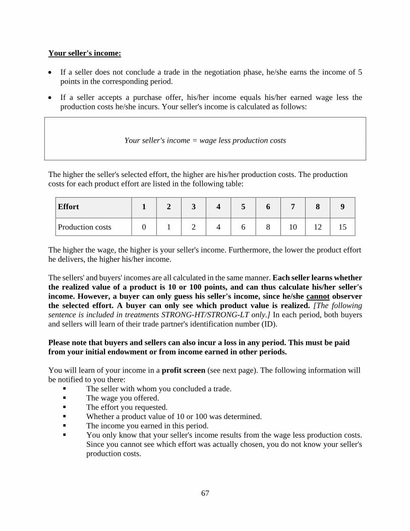
67

Your seller's income: • If a seller does not conclude a trade in the negotiation phase, he/she earns the income of 5

points in the corresponding period.

• If a seller accepts a purchase offer, his/her income equals his/her earned wage less the production costs he/she incurs. Your seller's income is calculated as follows:

Your seller's income = wage less production costs

The higher the seller's selected effort, the higher are his/her production costs. The production costs for each product effort are listed in the following table:

Effort 1 2 3 4 5 6 7 8 9

Production costs 0 1 2 4 6 8 10 12 15

The higher the wage, the higher is your seller's income. Furthermore, the lower the product effort he delivers, the higher his/her income. The sellers' and buyers' incomes are all calculated in the same manner. Each seller learns whether the realized value of a product is 10 or 100 points, and can thus calculate his/her seller's income. However, a buyer can only guess his seller's income, since he/she cannot observer the selected effort. A buyer can only see which product value is realized. [The following sentence is included in treatments STRONG-HT/STRONG-LT only.] In each period, both buyers and sellers will learn of their trade partner's identification number (ID). Please note that buyers and sellers can also incur a loss in any period. This must be paid from your initial endowment or from income earned in other periods. You will learn of your income in a profit screen (see next page). The following information will be notified to you there: The seller with whom you concluded a trade. The wage you offered. The effort you requested. Whether a product value of 10 or 100 was determined. The income you earned in this period. You only know that your seller's income results from the wage less production costs.

Since you cannot see which effort was actually chosen, you do not know your seller's production costs.

68

[Text on screen: Period 1 of 15 / Remaining time [sec] / Your identification number / You concluded the following trade / Your seller's ID / Wage / Requested effort / Realized value of the product / Your income = / Continue] Please enter all the information in the enclosed documentation sheet. Once the profit screen disappears, the period is over. The negotiation phase of the next period then begins. [The following sentence is included in treatments MEDIUM-HT/MEDIUM-LT only.] You will receive a new, randomly determined identification number for the next period, as will all other participants in the study. Once you have finished looking at the profit screen, please press the "continue" button. The sellers also have a profit screen where they are also informed about the information above. The sellers see their buyers' ID, the wage, the requested and actual product effort, whether the realized product value is 10 or 100 points, and the income for the seller and buyer that results. The study does not begin until all participants are completely informed about the study procedure. In order to confirm this, we ask that you solve a few practice questions. Furthermore, we will conduct two test periods of the negotiation phase so that you can become more familiar with the computer. These test periods will not be included in the final result and will not be paid out. After the test periods, the study will begin, lasting for a total of 15 periods.

69

[Treatments MEDIUM-HT/STRONG-HT:]

Example Before the present study begins, we would like to inform you of the study results that we observed in a past session. You can use this information when you make your decisions today. The bars in the left chart show the average effort that the sellers chose for the various wages. The left diagram shows that a seller on average selected an actual effort of 1.1 for a wage offer up to 9. By offers from 10 up to and including 19, effort of 2.6 was selected, for the range from 20 to 29 a effort of 3.6, and for wages from 30 to 39 a effort of 5.3. An average effort of 8.2 was selected for wages of 40 or higher. You can clearly see that the selected effort increases on average if the wage increases.

Sellers' effort selection Buyers' income

The line in the graph on the right emphasizes the correlation between wage and income that is realized with these effort values. For wages up to 9, the effort is only 1.1, but a lower wage is also paid. On average, a buyer's income is approximately 13 points. If, for example, wages from 20 to 29 are paid and the average effort is 3.6, an income of 19 results. Although the wage paid is considerably higher, a total higher income results since the average effort is also considerably higher. For wages of 40 or more, a buyer realizes an average income of 34 points.

70

[Treatments MEDIUM-LT/STRONG-LT:]

Example Before the present study begins, we would like to inform you of the study results that we observed in a past session. You can use this information when you make your decisions today. The bars in the left chart show the average effort that the sellers chose for the various wages. The left diagram shows that a seller on average selected an actual effort of 1.4 for a wage offer up to 9. By offers from 10 up to and including 19, effort of 1.6 was selected, for the range from 20 to 29 a effort of 2.8, and for wages from 30 to 39 a effort of 3.1. An average effort of 1 was selected for wages of 40 or higher. You can see that the selected effort barely increases on average if the wage increases.

Sellers' effort selection Buyers' income

The line in the graph on the right emphasizes the correlation between wage and income that is realized with these effort values. For wages up to 9, the effort is only 1.4, but a lower wage is also paid. On average, a buyer's income is approximately 14 points. If, for example, wages from 20 to 29 are paid and the average effort is 2.8, an income of 12 results. Although the wage paid is somewhat higher, a total lower income results since the wage paid is considerably higher. For wages of 40 or more, a buyer incurs a loss in excess of 20 points.

71

Practice questions Please solve these questions completely and show how you reached your answer. If you have questions, please raise your hand. False answers have no consequence for your payment at the end of the study.

Question 1 You did not make a purchase offer in a period. How high is your income in the period?

Your income = Question 2: Your purchase offer with a wage of 30 and a requested effort of 9 is accepted.

Your income when the value of the product is 100 equals = Your income when the value of the product is 10 equals = Your seller's income = How great is the probability that the value of the product for you is 100 points if the seller selects an actual effort of 8? How high is your seller's income in this case?

Question 3: Your purchase offer with a wage of 60 and a requested effort of 9 is accepted.

Your income when the value of the product is 100 equals = Your income when the value of the product is 10 equals = How great is the probability that the value of the product for you is 100 points if the seller selects an actual effort of 6? How high is your seller's income in this case?

72

Question 4: Your purchase offer with a wage of 10 and a requested effort of 2 is accepted.

Your income when the value of the product is 100 equals = Your income when the value of the product is 10 equals = How great is the probability that the value of the product for you is 100 points if the seller selects an actual effort of 5? How high is your seller's income in this case?

Question 5: Your purchase offer with a wage of 10 and a requested effort of 6 is accepted.

Your income when the value of the product is 100 equals = Your income when the value of the product is 10 equals = How great is the probability that the value of the product for you is 100 points if the seller selects an actual effort of 2? How high is your seller's income in this case?

Question 6 A seller did not accept a purchase offer in a negotiation phase. How high is this seller's income in this period?

Seller's income = Question 7 You made several purchase offers in a negotiation phase. None of these offers were accepted by a seller. How high is your income in this period?

Your income =

73

Question 8: Look at the example on page 9 of these instructions that provides information about a past session of this study. How did the seller's income change when the offered wage increased?

□ The income increased. □ The income decreased

Explain briefly the reason for this correlation between a buyer's income and the wage offered. Please raise your hand when you have solved these practice questions. We will then come to your seat and check your answers.

74

C2. Seller Instructions

Instructions for sellers

You are now participating in an economic study. Please read the following instructions carefully. Here you will learn everything you need to know to participate in the study. Please raise your hand if you do not understand something. We will answer your question at your desk. You will receive an initial endowment of 20 Swiss francs at the beginning of the study. You can earn additional income during the study by earning points. The number of points you earn during the study depends on your choices and on those of the other participants. All the points you earn during the course of the study will be converted to Swiss francs at the end of the study. The following conversion rate applies:

10 points = 1 Swiss franc You will receive the monetary amount you earned during the study plus the 20 Swiss francs initial endowment in cash at the end of the study. The study is divided into individual periods. You must make decisions each period which you enter into the computer. There are a total of 15 periods. Please note that communication is strictly forbidden during the study. Furthermore, we inform you that you may only use those functions on the computer that are necessary for completing the study. Communication or playing with the computer lead to exclusion from the study. We remain at your disposal to answer any questions you might have. The 34 participants were divided into two completely independent groups of 17 participants each before the beginning of the study. You will only interact within your group of 17 participants during the study. The participants in each group of 17 are then divided into 10 sellers and 7 buyers each. You are a seller during the entire study. [Treatments STRONG-HT/STRONG-LT:] All participants have an identification number that they retain for the entire duration of the study. Your identification number is on the documentation sheet in front of you. [Treatments MEDIUM-HT/MEDIUM-LT:] All participants have an identification number that changes randomly in each period. [Identical instructions from here onwards.]

75

Short summary of the procedure of the study

Each buyer can trade a product with a seller in each period of the study. The seller realizes a profit if he/she obtains a sales wage that exceeds his/her production costs. The production costs depend on the effort of the product. The higher the effort of the product that the seller chooses, the higher are his/her production costs. The buyer realizes a profit if he/she pays less for the product than its value to him/her. The value of a product is either 100 points (the product is exceptionally good) or 10 points (the product just fulfills its objective). The higher the effort that the seller selects, the higher the probability that the value of the product for the buyer is 100 points. The study lasts a total of 15 periods. The procedure in an individual period is organized as follows: 1. Each period begins with a negotiation phase that lasts for three minutes. Buyers can make

purchase offers that sellers can accept during this time.

When making a purchase offer, a buyer must determine three things:

• the wage he/she offers; • the effort he/she desires; • and finally to which seller he/she is directing the purchase offer. Buyers can make two

types of purchase offers: private and public. Private purchase offers are only directed to one seller and can only be accepted by this seller. Public purchase offers are directed to all sellers and can thus be accepted by any seller.

A buyer can make as many purchase offers as he/she wants in each period. You as a seller can only accept one purchase offer at most per period. If you accept a seller's offer, you conclude a trade with this seller for this period. Buyers, too, can only conclude one trade at most in a period. As there are a total of ten sellers and seven buyers, some sellers will not be able to participate in each period.

2. After the negotiation phase, all sellers who have concluded a trade must determine the product

effort that they want to deliver to their buyer. As a seller, you must not respect the buyer's requested effort. After all of the sellers have selected their product effort, it will be determined whether the value for each buyer is 100 points or 10 points. The higher the seller's selected effort, the higher the probability that the value for the buyer is 100 points. Once these values have been determined, the earnings for this period are settled for this period. Then the next period begins.

The income from all 15 periods will be added together at the end of the study, converted to Swiss francs, and paid out together with the initial endowment in cash.

76

Detailed procedure of the study There are 7 buyers and 10 sellers in your group of 17. You are a seller for the entire study. You will enter your decisions on the computer during the study. The information below shows you in detail how you make your decisions in each period. 1. The negotiation phase Each period of the study begins with a negotiation phase. Each buyer can conclude a trade with one seller in the negotiation phase. To do this, buyers can make purchase offers to sellers. As a seller, you can accept one of the offers made to you in each period. You will see the following decision screen during each negotiation phase:

[Text on screen: Period 1 of 15 / remaining time / your identification number / private offers to you / from seller / wage / requested effort / public offers / from seller / wage / requested effort / accept / your seller / your wage / requested effort] • You see which period you are in at the upper left corner of the screen. The remaining time in

this negotiation phase appears in seconds at the upper right corner. The negotiation phase lasts three minutes (=180 seconds) in each negotiation phase. Once the time has expired, the negotiation phase is over. Further purchase offers may neither be made nor accepted in this period.

5

77

[Only treatments MEDIUM-HT/MEDIUM-LT, but not STRONG-HT/STRONG-LT, include the following bullet point:] • The next item you see is your identification number. This identification number is randomly

redetermined in each period. This applies to all study participants, i.e. for all sellers and for all buyers.

• As soon as you see the screen above, the negotiation phase is opened. You as a seller now have the opportunity to accept purchase offers the sellers make to you. There are two types of purchase offers that you can accept: • Private purchase offers to you

Each buyer may offer you private purchase offers. These offers are only made to you, and only you can accept them. No other sellers or buyers will learn about this offer. If you receive private offers, they appear on the left side of your screen under the title "private offers to you". The buyer's offer contains the following information: the identification number of the buyer who is making the offer, the wage he/she offers for the product, and the effort he/she desires. If you want to accept a private offer, first click on the line where the private offer is entered with the mouse. The corresponding offer will then be marked. If you want to definitely accept the offer, click on the "accept" button at the lower right corner. You can change your selection up until you click on the "accept" button.

• Public purchase offers

Each buyer can make public purchase offers. Public purchase offers are notified to all sellers. All sellers see all public purchase offers on their screens. Each seller can thus accept a public purchase offer. If a seller makes a public offer, it appears on the right side of your screen under the title "public offers". The offer again consists of the identification number of the buyer who is making the offer, the wage he/she offers for the product, and the effort he/she desires. All other sellers and buyers receive this information. If you want to accept a public offer, the same procedure as for the private offers applies. First click on the line where the offer is entered. If you want to accept the offer definitely, click on the "accept" button on the lower right side. You can change your selection up until you click on the "accept" button.

• As soon as you click on the "accept" button, you will see which offer you accepted on the bottom line of your screen.

• Each seller can only conclude one trade in a period. Once you have accepted a purchase

offer, you cannot accept any more offers.

78

All buyers must accept the following rules for their purchase offers:

• The buyer's offer may not be less than 0 and may not be greater than 100:

0 ≤ purchase offer ≤ 100 • A buyer's requested product effort cannot be less than 1 and cannot be greater than 9.

1 ≤ requested product effort ≤ 9

• Each buyer can make as many private and public purchase offers in each period as he/she wants to. Each purchase offer a buyer makes in a period can be accepted during the negotiation phase.

• Each buyer can only conclude one trade in each period. As soon as a buyer's purchase order

is accepted, he/she will learn which seller accepted this offer. Since each buyer can only conclude one trade in each period, his/her remaining purchase offers are automatically deleted. He/She also cannot make any other purchase offers.

• The negotiation period is over as soon as all seven buyers have concluded a trade or the three

minutes are up. • No buyer is forced to make a purchase offer, and no seller is forced to accept an offer. 2. Determination of the actual product effort Once the negotiation phase is over, all sellers who have concluded a trade must decide which product effort they want to deliver to their buyers. The product effort that your buyer requested in your offer is not binding for you as seller. You can select exactly the product effort your buyer requested, but you can also choose a higher or lower product effort. If you concluded a trade in a negotiation phase, the entry of the product effort appears on the following screen:

79

[Text on screen: Period 1 of 15 / remaining time [sec] / You accepted the following offer / from buyer / wage / requested effort / determine the actual effort / OK] • In order to select your actual product effort, enter the value for the effort in the field "determine

the actual effort" and click on the "OK" button. You can change your selection until you click on the "OK" button.

The effort you select must be an integer between one and nine.

1 ≤ actual product effort ≤ 9

5

80

How are the incomes calculated?

Your income: • If you do not conclude a trade in the negotiation phase, you will earn an income of 5 points

in the corresponding period. • If you accept a purchase offer, your income depends on the accepted purchase and the product

effort you select. Your income is calculated as follows:

Your income = wage less production costs

• The higher your effort, the higher are your production costs. The production costs for each product effort are listed in the following table:

Effort 1 2 3 4 5 6 7 8 9

Production costs 0 1 2 4 6 8 10 12 15

• The lower your selected effort, the higher is your income. Furthermore, the higher your

buyer's offered wage, the higher is your income. Your buyer's income: • If a buyer does not conclude a trade during the period in question, he/she will earn an income

of 0 points in the period.

• If one of his/her offers was accepted, his/her income depends on the wage he/she offers and whether a product value of 10 or 100 points is determined. The higher the effort the seller selects, the higher is the probability that the value of the product will be 100. Your buyer's income is calculated as follows:

Your income = 100 – wage, if the high product value is determined

Your income = 10 – wage if the low product value is determined

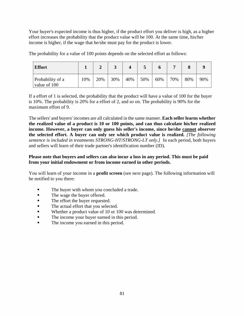
81

Your buyer's expected income is thus higher, if the product effort you deliver is high, as a higher effort increases the probability that the product value will be 100. At the same time, his/her income is higher, if the wage that he/she must pay for the product is lower. The probability for a value of 100 points depends on the selected effort as follows:

Effort 1 2 3 4 5 6 7 8 9

Probability of a value of 100

10% 20% 30% 40% 50% 60% 70% 80% 90%

If a effort of 1 is selected, the probability that the product will have a value of 100 for the buyer is 10%. The probability is 20% for a effort of 2, and so on. The probability is 90% for the maximum effort of 9.

The sellers' and buyers' incomes are all calculated in the same manner. Each seller learns whether the realized value of a product is 10 or 100 points, and can thus calculate his/her realized income. However, a buyer can only guess his seller's income, since he/she cannot observer the selected effort. A buyer can only see which product value is realized. [The following sentence is included in treatments STRONG-HT/STRONG-LT only.] In each period, both buyers and sellers will learn of their trade partner's identification number (ID). Please note that buyers and sellers can also incur a loss in any period. This must be paid from your initial endowment or from income earned in other periods. You will learn of your income in a profit screen (see next page). The following information will be notified to you there: The buyer with whom you concluded a trade. The wage the buyer offered. The effort the buyer requested. The actual effort that you selected. Whether a product value of 10 or 100 was determined. The income your buyer earned in this period. The income you earned in this period.

82

[Text on screen: Period 1 of 15 / remaining time / your identification number / You concluded the following trade / your buyer's ID / wage/ requested effort / actually selected effort / realized value of the product / your buyer's income / your income / continue] Please enter all the information in the enclosed documentation sheet. Once the profit screen disappears, the period is over. The negotiation phase of the next period then begins. [The following sentence is included in treatments MEDIUM-HT/MEDIUM-LT only.] You will receive a new, randomly determined identification number for the next period, as will all other participants in the study. Once you have finished looking at the profit screen, please press the "continue" button. The buyers also have a profit screen where they are informed about the past period. The buyers see their seller's ID, the wage, and the requested product effort. However, the buyers cannot observe the product effort that was actually chosen. The buyers only see if a product value of 10 or 100 was realized. The study will not begin until all participants are completely informed about the study procedure. In order to confirm this, we ask that you solve a few practice questions. Furthermore, we will conduct two test periods of the negotiation phase so that you can become more familiar with the computer. These test periods will not be included in the final result and will not be paid out. After the test periods, the study will begin, lasting for a total of 15 periods.

83

Practice questions Please solve these questions completely and show how you reached your answer. If you have questions, please raise your hand. False answers have no consequence for your payment at the end of the study.

Question 1 You did not accept a purchase offer in a period. How high is your income in the period?

Your income = Question 2: You accepted a purchase offer with a wage of 60 and a requested effort of 9. You select the actual effort of 9.

Your income = Your buyer's income when the value of the product is 100 equals = Your buyer's income when the value of the product is 10 equals = How great is the probability that the value of the product for you is 100 points if the seller selects an actual effort of 9?

Question 3: You have accepted purchase offer with a wage of 60 and a requested effort of 9. You choose an actual effort of 4.

Your income = Your buyer's income when the value of the product is 100 equals = Your buyer's income when the value of the product is 10 equals = How great is the probability that the value of the product for you is 100 points if the seller selects an actual effort of 4?

84

Question 4: You have accepted purchase offer with a wage of 40 and a requested effort of 2. You choose an actual effort of 5.

Your income = Your buyer's income when the value of the product is 100 equals = Your buyer's income when the value of the product is 10 equals = How great is the probability that the value of the product for you is 100 points if the seller selects an actual effort of 5?

Question 5: You have accepted purchase offer with a wage of 30 and a requested effort of 6. You choose an actual effort of 6.

Your income = Your buyer's income when the value of the product is 100 equals = Your buyer's income when the value of the product is 10 equals = How great is the probability that the value of the product for you is 100 points if the seller selects an actual effort of 6?

Question 6 A buyer made several purchase offers in a negotiation phase. None of these offers were accepted by a seller. How high is the buyer's income in the period in question?

Buyer's income = Please raise your hand when you have solved these practice questions. We will then come to your seat and check your answers.