the complementary use of theoretical structure prediction and x-ray
TRANSCRIPT
THE COMPLEMENTARY USE OF THEORETICAL STRUCTURE
PREDICTION AND X-RAY POWDER DIFFRACTION DATA IN
CRYSTAL STRUCTURE DETERMINATION
by
LIANA VELLA-ZARB
A thesis submitted toThe University of Birmingham
for the degree ofDOCTOR OF PHILOSOPHY
School of ChemistryThe University of Birmingham
September 2008

University of Birmingham Research Archive
e-theses repository This unpublished thesis/dissertation is copyright of the author and/or third parties. The intellectual property rights of the author or third parties in respect of this work are as defined by The Copyright Designs and Patents Act 1988 or as modified by any successor legislation. Any use made of information contained in this thesis/dissertation must be in accordance with that legislation and must be properly acknowledged. Further distribution or reproduction in any format is prohibited without the permission of the copyright holder.

TABLE OF CONTENTS
Chapter Title Page
I Acknowledgements i
II Abstract ii
III List of Tables iii
IV List of Figures v
1 Introduction 1
1.1 Background 1
1.2 Crystallinity and Crystal Packing 3
1.3 The Importance of Structure 7
1.4 Diffraction 8
1.4.1 X-ray Diffraction 8
1.4.2 Bragg’s Law 9
1.4.3 The Crystallographic Phase Problem 12
1.4.4 PXRD vs Single Crystal 12
1.5 Structure Determination from Powder Diffraction 14
1.5.1 Indexing 14
1.5.2 Space Group Assignment 15
1.5.3 Structure Solution Methods 16
1.5.4 Structure Refinement 17
1.6 Thermal Expansion 18
1.7 Polymorphism 20
1.8 Crystal Structure Prediction 22
1.8.1 Methodologies 22
1.9 Two-Way Relationship 26
1.10 Project Aims 27
Table of Contents Liana Vella-Żarb

1.11 References 28
2 Methodology 31
2.1 Automated Comparison 31
2.1.1 Rwp Calculation 31
2.1.2 PolySNAP 33
2.1.3 Compare 38
2.2 Low Temperature Data 42
2.3 References 42
3 Experimental 44
3.1 Instrumentation 44
3.2 Sample Effects 45
3.2.1 Transparency and Sample Contraction 46
3.2.2 Sample Displacement 49
3.2.3 Preferred Orientation 50
3.2.4 Sample Loss 51
3.3 Materials 52
3.4 References 52
4 Imidazole 53
4.1 Background 53
4.1.1 Crystal Structure 54
4.1.2 Crystal Structure Prediction 55
4.2 Results 57
4.2.1 Low Temperature Structures 57
4.2.2 Automated Comparison 60
4.2.2.1 Rwp 60
4.2.2.2 PolySNAP 63
4.2.2.3 Compare.x 68
4.3 Discussion 71
Table of Contents Liana Vella-Żarb

4.4 References 72
5 Chlorothalonil 73
5.1 Background 73
5.1.1 Crystal Structure of Form I 74
5.1.2 Crystal Structure Prediction 75
5.2 Results 77
5.2.1 Low Temperature Data 77
5.2.2 Automated Comparison 80
5.2.2.1 Rwp 80
5.2.2.2 PolySNAP 83
5.2.2.3 Compare.x 88
5.3 Discussion 91
5.4 References 93
6 5-Azauracil 94
6.1 Background 94
6.1.1 Crystal Structure 95
6.1.2 Crystal Structure Prediction 95
6.2 Results 98
6.2.1 Low Temperature Data 98
6.2.2 Automated Comparison 102
6.2.2.1 Rwp 102
6.2.2.2 PolySNAP 104
6.2.2.3 Compare.x 109
6.3 Discussion 115
6.4 References 117
7 DNA Bases 118
7.1 Adenine 118
7.1.1 Background 119
Table of Contents Liana Vella-Żarb

7.1.1.1 Experimental Polymorph Search 119
7.1.1.2 Computational Polymorph Search 119
7.1.2 Results 122
7.1.2.1 PolySNAP 122
7.1.2.2 Compare.x 129
7.1.2.3 Rwp 132
7.1.3 Structure Determination 135
7.1.4 Crystal Structure 140
7.1.4.1. Single-Crystal Structure Determination 141
7.1.5 Low Temperature Data 144
7.1.6 Discussion 146
7.2 Guanine 148
7.2.1 Background 148
7.2.1.1 Experimental Polymorph Search 149
7.2.1.2 Computational Polymorph Search 149
7.2.2 Results 153
7.2.2.1 PolySNAP 158
7.2.3 Low Temperature Data 164
7.2.4 Discussion 167
7.3 Adenine vs Guanine 168
7.3 References 170
8 Conclusions and Further Work 171
9 Appendices 174
A1 Rwp 174
A2 Imidazole 178
A3 Chlorothalonil 195
A4 5-Azauracil 210
A5 DNA Bases 229
Table of Contents Liana Vella-Żarb

ACKNOWLEDGEMENTS
This was one of the most important and formative experiences in my life, and I would never have done it without the help of some very special people.
First of all, my thanks and appreciation go to Maryjane for persevering with me as my tutor throughout the time it took me to complete this research and write the dissertation. Your support (and unlimited patience!) and the many conversations that clarified my thinking on this and so many other matters (from powders to grappa, and beyond!) were essential components of this journey. Thank you for your friendship and academic support - they mean a great deal to me.
I would also like to thank all the members of the CPOSS team, especially Sally Price and Panos Karamertzanis, who have generously given their time and expertise to better my work. Thank you for your contribution and good-natured support. Special thanks go to Chick Wilson for the many times he came to the rescue when I was about to give up....conferences would not have been the same without those late night pep talks!!
I want to thank my friends and colleagues in Birmingham: Adam especially, for taking on the brave task of printing out this dissertation for me and for making the office a happier place; Sam for being there from the start, even when I was almost homeless; Emma for the very special friendship; James for being like a brother to me; and all the members of Level 2 and Level 5. You’ve all left your footprint on my heart.
I cannot fail to mention my very dear “chemistry family” in Glasgow - Suzie, Lynne, Marc, Mar-tin, Duncan and Andy. You guys are the true definition of friendship - thank you for being the crazy fantastic people you are. I love you all to bits and getting to know you has made this expe-rience so much more valuable to me.
Finally, my sincere appreciation goes to my family in Malta. To Mama, who always seems to have unlimited supplies of energy, positivity, support and reassurance, and whose phonecalls helped me feel warm, safe and at home when I was going through a rough patch. Thank you for reading through all these pages, but most of all, thank you for making me feel like I was always part of a team. With you around, I will surely never walk alone. To Papinu, for all the little things he says which make a big difference to us, even though he thinks we aren’t listening. You once told me “Dare to think, dare to fail, dare to act, because sometimes it’s better to regret things done than things left undone”. This experience would have probably just been a secret dream had it not been for those words....And lastly to my dear brother Andrew whom I missed so much while I was away. Thank you for letting me nick your laptop while I was writing up, and for putting up with my general madness. Your maturity, determination and strength of character are an inspiration to me, and I can only hope that one day I might make you as proud of me as I am of you.
Acknowledgements Liana Vella-Żarb
i

ABSTRACT
The successful prediction of the crystal structure and symmetry of a material can give
valuable insight into many of its properties, as well as the feasibility of thermodynamically stable
polymorphs to exist. It is not uncommon, however, for numerous theoretical structures to be
found within a narrow energy range, making absolute characterisation of the crystal structure
impossible. The aim of this project was to investigate a number of structures from this scenario,
highlighting the key differences between three potential methods for the automated comparison of
predicted and experimental crystal structures.
This work was carried out by comparing the simulated powder diffraction patterns of
theoretical predicted crystal structures of small organic materials with their experimental powder
diffraction patterns, so that the experimentally identified structure could be automatically singled
out from the many calculated. The use of traditional agreement factors (eg. Rwp) was compared
with more sophisticated approaches namely PolySNAP, which uses principal-component analysis,
and Compare.x, an algorithm based on weighted cross-correlation. Five structures were analysed,
two of which had not been previously characterised. As the structure prediction calculations are
carried out at 0K, and experimental data were collected over a range of temperatures (10K-293K),
the effect of the resulting variations in lattice parameters on the automated processes is discussed.
In all cases, Rwp has proven to be a poor and unreliable discriminator in the comparison of
predicted and experimental structures. The more contemporary methods based on PolySNAP and
Compare.x both gave encouraging results when used to study the three known structures
imidazole, chlorothalonil and 5-azauracil, and they have consequently been used in the successful
solution of the two previously unknown structures adenine and guanine. A difference in
sensitivity in the matching of data collected at different temperatures between the latter
approaches was noted. It was found that although there is considerable overlap between the two
methods, they are not absolutely interchangeable, and this distinction may be exploited in future
work where more case-specific comparisons are carried out. Automated comparison techniques
cannot yet replace visual comparison completely, but they reduce it drastically. Ultimately,
comparisons made computationally serve as a complement to human judgement, but they may not
yet eliminate it.
Abstract Liana Vella-Żarb
ii

LIST OF TABLES
TableNumber
Title Page
1.1 The seven crystal systems 5
3.1 Calculated peaks for NaCl with a change in temperature at different wavelengths 49
3.2 List of data sets collected for each material studied 52
4.1 Unit cell parameters of lowest energy predicted structure and determined from experimental data, and published unit cell dimensions for imidazole with changing temperature
58
4.2 Structures with lowest Rwp identified at each temperature 60
4.3 Structures with highest correlation coefficient [P(x)] at each temperature, and the difference to the value obtained for the correct structure [P(ak34)]
64
4.4 Structures with highest correlation coefficient [C(x)] at each temperature, and the difference to the value obtained for the correct structure [C(ak34)]
68
4.5 Comparison of the ability of the three methods in the automated identification of the correct predicted structure
71
5.1 Five lowest energy structures for chlorothalonil minimised using the ANI potential2
76
5.2 Unit cell parameters of the lowest energy predicted structure, those determined from experimental data, and published unit cell dimensions for chlorothalonil with changing temperature
78
5.3 Structures with lowest Rwp identified at each temperature 80
5.4 Structures with highest correlation coefficient [P(x)] at each temperature, and the difference to the value obtained for the correct structure [P(fc45)]
84
5.5 Structures with highest correlation coefficient [C(x)] at each temperature, and the difference to the value obtained for the correct structure [C(fc45)]
88
5.6 Comparison of the ability of the three methods in automated identification of the correct predicted structure
91
List of Tables Liana Vella-Żarb
v
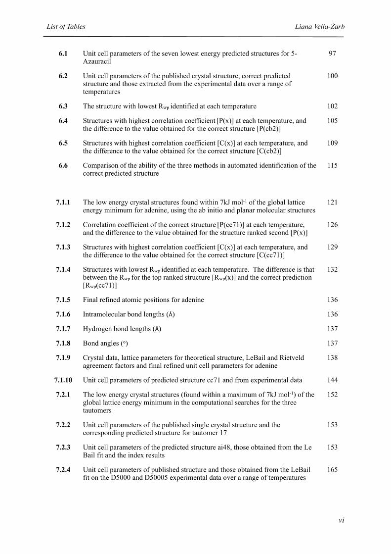
6.1 Unit cell parameters of the seven lowest energy predicted structures for 5-Azauracil
97
6.2 Unit cell parameters of the published crystal structure, correct predicted structure and those extracted from the experimental data over a range of temperatures
100
6.3 The structure with lowest Rwp identified at each temperature 102
6.4 Structures with highest correlation coefficient [P(x)] at each temperature, and the difference to the value obtained for the correct structure [P(cb2)]
105
6.5 Structures with highest correlation coefficient [C(x)] at each temperature, and the difference to the value obtained for the correct structure [C(cb2)]
109
6.6 Comparison of the ability of the three methods in automated identification of the correct predicted structure
115
7.1.1 The low energy crystal structures found within 7kJ mol-1 of the global lattice energy minimum for adenine, using the ab initio and planar molecular structures
121
7.1.2 Correlation coefficient of the correct structure [P(cc71)] at each temperature, and the difference to the value obtained for the structure ranked second [P(x)]
126
7.1.3 Structures with highest correlation coefficient [C(x)] at each temperature, and the difference to the value obtained for the correct structure [C(cc71)]
129
7.1.4 Structures with lowest Rwp identified at each temperature. The difference is that between the Rwp for the top ranked structure [Rwp(x)] and the correct prediction [Rwp(cc71)]
132
7.1.5 Final refined atomic positions for adenine 136
7.1.6 Intramolecular bond lengths (Å) 136
7.1.7 Hydrogen bond lengths (Å) 137
7.1.8 Bond angles (o) 137
7.1.9 Crystal data, lattice parameters for theoretical structure, LeBail and Rietveld agreement factors and final refined unit cell parameters for adenine
138
7.1.10 Unit cell parameters of predicted structure cc71 and from experimental data 144
7.2.1 The low energy crystal structures (found within a maximum of 7kJ mol-1) of the global lattice energy minimum in the computational searches for the three tautomers
152
7.2.2 Unit cell parameters of the published single crystal structure and the corresponding predicted structure for tautomer 17
153
7.2.3 Unit cell parameters of the predicted structure ai48, those obtained from the Le Bail fit and the index results
153
7.2.4 Unit cell parameters of published structure and those obtained from the LeBail fit on the D5000 and D50005 experimental data over a range of temperatures
165
List of Tables Liana Vella-Żarb
vi

LIST OF FIGURES
Figure Number
Title Page
1.1 Scheme VII from Hooke’s Micrographia, 1665 2
1.2 Development of the unit cell 3
1.3 Unit cell notation 4
1.4 Figure illustrating the four lattice types 6
1.5 Bragg scattering of X-rays from parallel planes 9
1.6 Direct lattice and the corresponding reciprocal lattice 11
1.7 Diffraction from single crystal and powder 13
1.8 Examples of crystal energy landscapes 24
2.1 Diagram showing observed peak, calculated peak and difference plot 32
2.2 Example of a dendrogram 38
3.1 Diagram showing the effect of specimen transparency or specimen displacement on the radius of the focusing circle
47
3.2 Diagram showing the effect of specimen transparency or specimen displacement on the diffraction surface
48
3.2 Diagram showing the techniques used to mount the sample onto the sample holder for collection of low-temperature data
50
4.1 Imidazole (1,3-diaza-2,4-cyclopentadiene) 53
4.2 Imidazole molecules forming chains parallel to the c axis 54
4.3 A view down the c axis 55
4.4 The distribution of low energy structures found in the search for minima in the lattice energy of imidazole
56
4.5 Section of superimposed powder diffraction data at all temperatures showing selected peaks shifting towards the right with decreasing temperature
57
4.6 Graph showing the percentage change in unit cell dimensions with temperature 59
4.7 Rwp values for each predicted structure at each temperature 61
List of Figures Liana Vella-Żarb
v

4.8 Rwp values for each predicted structure against the D5000 data at room temperature
62
4.9 Dendrogram showing similarity clusters for imidazole predicted and experimental powder patterns
63
4.10 Correlation coefficients of all 65 structures at each temperature 65
4.11 Correlation coefficients of all 65 structures against the D5000 data 66
4.12 Powder diffraction patterns for five selected predicted structures and the experimental structure at room temperature
67
4.13 Correlation coefficients of all 65 structures at each temperature 69
4.14 Correlation coefficients of all 65 structures against the D5000 data 70
4.15 Difference in correlation coefficients between ak34 and the structure with the next highest correlation
72
5.1 Chlorothalonil (2,4,5,6-tetrachloro-1,3-benzenedicarbonitrile) 73
5.2 A view of the crystal structure of chlorothalonil down the a axis 74
5.3 Packing diagram showing the herringbone structure 74
5.4 The distribution of low energy structures found in the search for minima in the lattice energy of chlorothalonil
76
5.5 Section of superimposed powder diffraction data at all temperatures showing peaks shifting towards the right with decreasing temperature
77
5.6 Graph showing the percentage change in unit cell dimensions with temperature 79
5.7 Rwp values for each structure at each temperature 81
5.8 Rwp values for each structure against the D5000 data at room temperature 82
5.9 Dendrogram showing similarity clusters for chlorothalonil predicted and experimental powder patterns
83
5.10 Powder diffraction patterns for five selected predicted structures and the experimental structure at room temperature
85
5.11 Correlation coefficients of all 22 structures at each temperature 86
5.12 Correlation coefficients of all 22 structures against the D5000 data at room temperature
87
5.13 Correlation coefficients of all 22 structures at each temperature 89
5.14 Correlation coefficients of all 22 structures against the D5000 data at room temperature
90
5.15 Difference in correlation coefficients between fc45 and the structure with the net highest correlation
92
List of Figures Liana Vella-Żarb
vi

6.1 5-Azauracil (1,3,5-triazine-2,4(1H,3H)-dione) 94
6.2 5-Azauracil molecules forming chains along the b axis 95
6.3 A view down the a axis 96
6.4 The distribution of the lowest energy structures found in a search for minima in the lattice energy of 5-azauracil
97
6.5 Simulated powder patterns for the published single crystal structure, the correct predicted structure cb2, predicted structure aq62, and the experimental data recorded at room temperature
99
6.6 Section of superimposed powder diffraction data at all temperatures showing peaks shifting towards the right with decreasing temperature
101
6.7 Graph showing the percentage change in unit cell dimensions with temperature 101
6.8 Rwp values for each predicted structure at each temperature 103
6.9 Dendrogram showing similarity clusters for 5-azauracil predicted and experimental powder patterns
104
6.10 Correlation coefficients of all 49 structures at each temperature 106
6.11 Correlation coefficients of all 49 structures against the D5000 data 107
6.12 Powder diffraction patterns for four selected predicted structures and the experimental structure at room temperature
108
6.13 Correlation coefficients of all 49 structures at each temperature 110
6.14 Correlation coefficients of all 49 structures against the D5000 data 111
6.15 Powder diffraction patterns for fa41 and the experimental structure at 10K and 100K
112
6.16 Powder diffraction patterns for cb117 and the experimental structure at room temperature
113
6.17 Powder diffraction patterns for fa53 and the D5000 experimental structure 114
6.18 Difference in correlation coefficients between cb2 and the structure with the next highest correlation
116
7.1.1 Adenine (6-aminopurine) 118
7.1.2 The results of both computational searches (ab initio and planar) showing the predicted structure corresponding to the experimental form
120
7.1.3 The three different hydrogen bonded sheet structures present in the low energy structures in both computational polymorph searches on adenine
122
7.1.4 Dendrogram showing similarity correlation clusters for predicted adenine and experimental adenine powder diffraction patterns
123
7.1.5 Correlation coefficients of all 33 predicted structures with room temperature (D5000) data
124
List of Figures Liana Vella-Żarb
vii

7.1.6 Powder diffraction patterns for two selected predicted structures and the experimental data (D5000) at room temperature
125
7.1.7 Powder diffraction patterns for two selected predicted structures and the experimental data (D5005) at all temperatures
127
7.1.8 Correlation coefficients of all 33 predicted structures at each temperature 128
7.1.9 Correlation coefficients of all 33 structures at each temperature 130
7.1.10 Correlation coefficients of all 33 predicted structures with room temperature (D5000) data
131
7.1.11 Rwp values for each predicted structure at each temperature with the D5005 data 133
7.1.12 Rwp values for each predicted structure with the D5000 data 134
7.1.13 Atomic positions 135
7.1.14 Rietveld refinement of adenine against the D5000 room temperature data 139
7.1.15 (a) Crystal packing of adenine, (b) sheet made of hydrogen-bonded rings form-ing a honeycomb pattern and (c) R²2 (8) and R²2 (9) motifs
140141
7.1.16 Two components of the adenine molecule disordered about a 2-fold rotation axis passing through N1 and the midpoint of C4 and C4i
142
7.1.17 A single two-dimensional hydrogen-bonded layer in the ac plane, showing all disorder components
142
7.1.18 Powder diffraction patterns simulated from the single-crystal structure (SX) and the experimental data at room temperature (RT)
143
7.1.19 Section of superimposed powder diffraction data at all temperatures showing selected peaks shifting towards the right with decreasing temperature
145
7.1.20 Graph showing the percentage change in unit cell dimensions with temperature 146
7.2.1 Guanine (2-amino-1,7-dihydro-6H-purin-6-one); 2-amino-6-oxypurine 148
7.2.2 The three tautomers for guanine 149
7.2.3 The results of the computational search for Tautomer 17 150
7.2.4 The results of the computational search for Tautomer 19 151
7.2.5 The results of the computational search for Tautomer 39 151
7.2.6 Powder diffraction pattern of predicted structure ai48 and the experimental data at room temperature
154
7.2.7 Le Bail fit of the experimental data at room temperature using parameters from structure ai48 as a starting point
155
7.2.8 Powder diffraction patterns of the single crystal structure, Toni Llinas’ structure and the experimental data at room temperature (a) full range; (b) selection
156157
7.2.9 Dendrogram showing similarity correlation clusters for predicted Tautomer 17 structures
158
List of Figures Liana Vella-Żarb
viii

7.2.10 Dendrogram showing similarity correlation clusters for predicted Tautomer 19 structures
159
7.2.11 Dendrogram showing similarity correlation clusters for predicted Tautomer 39 structures
159
7.2.12 Correlation coefficients of all predicted structures for Tautomer 17 at each experimental temperature and against the published structure (SX) and Toni Llinas’ data (Toni)
160
7.2.13 Correlation coefficients of all predicted structures for Tautomer 19 at each experimental temperature and against the published structure (SX) and Toni Llinas’ data (Toni)
161
7.2.14 Correlation coefficients of all predicted structures for Tautomer 39 at each experimental temperature and against the published structure (SX) and Toni Llinas’ data (Toni)
162
7.2.15 Powder diffraction patterns of predicted structures dd94, am92 and ai48 and the experimental structure at room temperature
163
7.2.16 Graph showing the percentage change in unit cell dimensions with temperature 166
7.2.17 Section of superimposed powder diffraction data at all temperatures showing selected peaks shifting towards a higher 2θ with decreasing temperature
166
7.2.18 DNA monomer showing guanine as tautomer 19 167
7.3.1 Crystal structure of guanine 168
7.3.2 Crystal structure of adenine 169
List of Figures Liana Vella-Żarb
ix

1. INTRODUCTION
1.1 Background
Crystals have been objects of fascination throughout the history of mankind, with mystical,
magical and even medicinal properties being attributed to them over the ages. Evidence of this
are the carvings depicting their use as ornaments, amulets and charms, discovered by
archaeologists in prehistoric tombs. However, crystals were not only used as ornaments in their
natural form. They were also refined and used, together with sound, to produce artificial light, as
the French explorer Captain Auvergne reported on his return from Tibet. This effect is also
observed in New Grange in Ireland, built circa 3200BC in honour of Oenghus, god of love.
Covering the facade of this temple is white quartz, a material of particular interest in the history of
crystallography, since it was the first to be described as a “crystal”. The term, which comes from
the Greek word κρύσταλλοσ meaning frozen droplet, was chosen because of the icy appearance of
quartz.
As crystals and their structure lie at the core of this project, a brief overview of how the study
of crystals came to be the important area of solid state chemistry it is today, is due. The term
“crystallography” derives from the two words κρύσταλλοσ and γράφιµο , the latter meaning
“writing”. It thus follows that documenting the description of crystals as accurately and
thoroughly as possible constitutes the main focus of every crystallographer’s job description.
Although crystals had been admired for their external appearance for millennia, it wasn’t until
1665 that the first connection between external form and internal order was made by Robert
Hooke, who suggested that the different shapes of crystals could arise from the packing together
of spheres or globules1 [Figure 1.1]. In 1669, Nicolaus Steno cut sections across quartz crystals,
showing that regardless of the size of the faces on the crystals, they were always inclined to one
another at constant dihedral angles2.
Introduction Liana Vella-Żarb
1

Figure 1.1. “Scheme VII” from Hooke’s Micrographia, 1665, showing hypothetical crystal structures arising from packing of globules.
Introduction Liana Vella-Żarb
2

Later that century, Guglielmini made some observations about the constant nature of cleavage
directions in crystals. He suggested the presence of crystal planes along which the crystal could
be caused to split regularly, and this led him to believe that the building blocks of crystals
suggested by Hooke must themselves be miniature crystals with plane faces3. In 1784, in his
work entitled Essay d’une théorie sur la structure des crystaux appliquée a plusieurs genres de
substances crystallisées, René Just Haüy reported experiments suggesting that continued cleavage
would ultimately lead to a smallest possible unit (molécule intégrante), by a repetition of which
the whole crystal is built2. If each of these units is replaced by a point, regardless of its contents,
and adjacent points are joined, the resulting structural unit is a complete representation of the
contents of the whole structure [Figure 1.2]. Thus Haüy, having given birth to the concept of the
unit cell, is deemed the “Father of Crystallography”.
Figure 1.2. Development of the “unit cell” by replacing cubes with points.
1.2 Crystallinity and Crystal Packing
A material can be considered crystalline if its constituent molecules, atoms or ions exhibit
long-range three-dimensional periodic order. This structural arrangement can be described in a
complete manner by taking into consideration the repeating unit (the unit cell), its contents (the
structural motif) and the manner in which the unit cell is repeated (the symmetry).
Introduction Liana Vella-Żarb
3

The unit cell can be described by three vectors a, b and c which are the lattice vectors and
form a parallelepiped. The directions specified by these vectors can be represented by the X, Y
and Z orthogonal axes respectively, while α, β and γ are the angles between them [Figure 1.3].
αβγ
a
b
c
AB
C
Figure 1.3 Unit cell notation. The directions of vectors a, b and c are the X, Y and Z axes.
A crystallographic plane is defined by three lattice points, or indices (hkl). Planes parallel to
one of the three axes X, Y or Z are defined by indices of the type (0kl), (h0l) and (hk0)
respectively, while planes parallel to faces A, B and C of the unit cell are represented by indices of
the type (h00), (0k0) and (00l) respectively. While some crystals have a centre of symmetry
illustrated by the occurrence of similar faces of the same size and shape lying in parallel pairs on
opposite sides of the crystal, some others do not. Such crystals exhibit a different type of
arrangement, defined by reflection, translation or rotational symmetry elements, which can only
be combined together in a restricted number of ways that are consistent with each other. For a
single molecule, the total collection of all its symmetry operations is called its point group, and
each of these point groups is characterised by a number of specific properties. Since rotation in
crystal elements can only exhibit a maximum order of six, there are 32 possible ways in which
symmetry factors can be combined. In order to satisfy the criterion that the unit cell must be
capable of repetition in space without leaving any gaps, there is a natural limit to the types of unit
cell that can be used to build a crystal. The 32 point groups give rise to only seven different unit
cell shapes, and these form the basis of the classification of crystals into seven distinct groups or
crystal systems [Table 1.1].
Introduction Liana Vella-Żarb
4

Table 1.1 The seven crystal systems.
Crystal system Essential symmetry Restrictions on unit cell Bravais lattices
Cubic
Hexagonal
Trigonal (Rhombohedral)
Tetragonal
Orthorhombic
Monoclinic
Triclinic
Four three-fold rotation axes
a = b = cα = β = γ = 90o
P, I, F
One six-fold rotation
a = b ≠ cα = β = 90o ; γ = 120o
P
One three-fold rotation
a = b = cα = β = γ ≠ 90o
P (R)
One four-fold rotation
a = b ≠ cα = β = γ = 90o
P, I
Three two-fold rotations and/or mirror planes
a ≠ b ≠ cα = β = γ = 90o
P, C (A), I, F
One two-fold axis and/or mirror plane
a ≠ b ≠ cα = γ = 90o ≠ β
P, C (I)
None a ≠ b ≠ cα ≠ β ≠ γ
P
For crystal structures showing more than just translational symmetry, a unit cell containing
more than just one lattice point is chosen by convention. This is merely done for convenience, as
the resultant unit cell geometry would display the symmetry more clearly. Unit cells with one
lattice point are referred to as primitive (P), and those with more than one lattice point are called
centred. The various crystal systems can exhibit different kinds of centering: side-centred, having
lattice points at the centres of opposite pairs of faces (A, B, or C depending on which faces are
centred), face-centred, having lattice points at the centres of all faces (F), and body-centred,
having a lattice point at the centre of the cell (I) [Figure 1.4]. The different possible combinations
of cell symmetry with primitive and centred cell geometries result in 14 lattice types, known as
Bravais lattices. The presence of translation coupled with the other symmetry functions, also
gives rise to compound symmetry elements such as glide planes and screw axes. A glide plane is
the combination of a translation with a mirror reflection, while the combination of a translation
with a rotation changes the rotational axes to a screw axis. Combining all the possible symmetry
operations in the solid state with Bravais lattices gives rise to 230 distinct arrangements, known as
space groups. Every crystal structure can be classified under one of these space groups.
Introduction Liana Vella-Żarb
5

The first part of a space group symbol denotes the lattice type [Figure 1.4], and is denoted by a
capital letter P, C (B or A), I or F. These refer to primitive, face-centred, body-centred, and all-
face-centred. The second part of the space group describes the symmetry within the unit cell.
This is irreducible representation in that only the minimum symmetry is specified in order to
identify the space group.
P I
F C
Figure 1.4 Figure illustrating the four lattice types.
In a purely translational lattice, the repeat unit of a crystal structure is either one complete unit
cell (primitive cells) or a well-defined fraction of it (A, B, C, or I centering). If other symmetry
elements are present, then this would relate atoms or molecules within the unit cell to each other.
In this case, therefore, the unique part of the crystal structure usually corresponds to a fraction of
the unit cell, and it is dependent on the amount of symmetry present. This portion is called the
asymmetric unit of the structure, and by means of translation, rotation, inversion and reflection
symmetry elements, it generates the entire unit cell and, consequently, the complete crystal
structure.
Introduction Liana Vella-Żarb
6

1.3 The Importance of Structure
In this context, the term “structure” refers to the relative positions of the atoms or ions making
up the material, i.e. it is a geometrical description of bond lengths, bond angles, torsion angles,
non-bonded distances, etc. This enables crystallographers to represent the structure graphically,
satisfying the γράφιµο part of their title. However, knowledge about the structure of crystalline
materials goes beyond their pictorial importance. The structure of a crystalline system may be
used to understand its physical and chemical properties, including any magnetic or optical
behaviour3, and is thus of great use. Insight into the crystal structure of materials has applications
in various scientific fields: the characterisation of proteins and pigments in biology;
characterisation and development of non-linear optical materials, polymers and superconductors
in physics4,5; the reactivity and structure-energy relationships of newly-synthesised compounds in
chemistry5; and the characterisation of drugs and bioactive materials, as well as polymorph
investigation in pharmacy6, to name a few. In the case of pharmaceuticals, most of which are
administered in crystalline form, the crystal geometry of the active ingredient and its excipients
directly affect the drug’s bioavailability, and consequently its activity and toxicity. This particular
application also raises awareness about the impact of possible polymorphs having different
physico-chemical properties, both on industry, but more importantly, also in the body.
Throughout the ages, the study of the structure of crystals has made use of a wide variety of
experimental tools, depending on their availability. Steno’s slicing experiment, which gave rise to
the notion of the constancy of angles between corresponding faces on a crystal, later prompted
Rome de L’Isle (1772)7 to take a large number of measurements using a contact goniometer (a
form of protractor attached to a bar) in an attempt to prove this. It wasn’t until 1809 that
Wollaston7 invented the reflecting goniometer, which enabled the measurement of interfacial
angles more accurately. This subsequently led to the development of the single- and two-circle
goniometers, the latter having been independently invented by Miller (1874), Fedorov (1889) and
Goldschmidt (1893)7. The use of these tools in crystal structure determination was very popular,
until Max von Laue demonstrated the diffracting properties of X-rays in 19128.
Introduction Liana Vella-Żarb
7
1.4 Diffraction
Nowadays, structure analysis relies mostly on the interaction of a material with X-rays,
electrons, or neutrons, by measuring its emission or absorption of radiation. If the wavelength is
fixed (a condition known as monochromatic (single-wavelength, literally meaning single-
coloured) radiation), the variation of intensity with direction is measured, and from these
measurements it is possible to deduce the positions of the atoms in the sample. The variation in
intensity, or scattering, of monochromatic radiation, results from interference effects, more
commonly known as diffraction. Although the diffraction theory applies to all types of radiation,
only X-ray scattering is of relevance to this project, and it will therefore be discussed in further
detail.
1.4.1 X-ray Diffraction
X-rays can be described as electromagnetic radiation having a wavelength of the order of
10-10m (1Å). They were first described by Röntgen in 18957, but due to the limitations in the
optical instruments available at the time, he could not perform any experiments to measure
interference, reflection or refraction. It wasn’t until several years later that Prof Arnold
Sommerfield measured an X-ray wavelength of about 0.4Å. Inspired by discussions with Paul
Ewald, who was a PhD student with Prof Sommerfield at the time, Max von Laue suggested the
use of crystals as natural lattices for diffraction. W. Friedrich and P. Knipping, two of Röntgen’s
students, performed the experiment on a crystal of copper sulphate, and the beams were recorded
photographically. Their results were published in 19129.
These findings stirred interest in William L. Bragg, then a student in Cambridge. He noted the
geometrical shapes in Friedrich and Knipping’s photographs, and believed that this diffraction
could be regarded as cooperative reflections by the internal planes of the crystal. Only a year
later, in 1913, Bragg and von Laue used X-ray diffraction patterns to determine the structures of
KBr, KI, KCl and NaCl10.
A simple demonstration of the method by which X-rays are generated is the standard “X-ray
tube”. This produces electrons by passing an electrical current through a wire filament, accelerates
Introduction Liana Vella-Żarb
8

them to a high velocity, and directs them onto a cooled metal target (Mo, Cu, Fe, Cr). As they hit
the metal, the electrons decelerate rapidly, and this causes most of their kinetic energy to be
converted to heat and lost. However, some of this energy interacts with the target metal atoms to
produce X-rays. If an electron in a core atomic orbital is ionised (displaced), an electron from a
higher-energy orbital will replace it, and the subsequent drop in energy will result in the emission
of an X-ray photon. These particles of energy oscillate and can therefore be characterised by their
wavelength (the distance between peaks), the number of peaks that pass a point per unit time
(frequency) or by their energy E. If electrons in different orbitals are displaced, a difference in
energy would cause the generation of a different wavelength, even though the target metal is the
same, eg. In the case of Cu Kα (λ = 1.5418 Å) the transition of an electron from the 2p orbital of
the L energy level to the 1s orbital on K emits α radiation, while with Cu Kβ (λ = 1.3922 Å)
emission of β radiation results from the transition of a 3p electron to K11.
As an X-ray photon impinges upon a crystalline solid, it will either travel straight through it or
interact with the electric field due to the electrons in the material, and thus scatter. The electron
densities of all the atoms that lie in the path of an X-ray beam contribute to its scattering, causing
interference (constructive or destructive) between the X-ray waves. This is X-ray interference, or
X-ray Diffraction.
1.4.2 Bragg’s Law
O
E
1
BD
A
θ2
3
1’
F
C
θ2’
3’θ d
hkl
hkl
hkl
Figure 1.5 Bragg scattering of X-rays from parallel planes, with d representing interplanar spacing.
Introduction Liana Vella-Żarb
9

In 1913, Bragg showed that every diffracted beam that can be produced by a crystal face at a
particular angle of incidence can be geometrically considered to be a reflection from sets of
parallel planes passing through lattice points. This therefore requires that the angles of incidence
and reflection be equal, and that the incoming and outgoing beams and the normal to the
reflecting planes must themselves be in one plane [Figure 1.5]. The Miller Indices (hkl) are three
integers that describe the orientation of a plane with respect to the three unit cell edges. The
spacing dhkl between successive planes is determined by the lattice geometry and is therefore a
function of the unit cell parameters where V is the unit cell volume [Equation 1.1].
dhkl = V[h2b2c2sin2α + k2a2c2sin2β + l2a2b2sin2γ + 2hlab2c(cosαcosγ - cosβ)
+ 2hkabc2(cosαcosβ - cosγ) + 2kla2bc(cosγcosβ - cosα)]-½
Equation 1.1
Diffraction from these planes will only give rise to constructive interference if the path
difference between radiation scattered from adjacent planes is equal to a whole number of
wavelengths. This is Bragg’s Law, and it can be expressed as
nλ = 2dhkl sinθhkl
Equation 1.2
where λ is the wavelength of the incident radiation, 2θhkl is the angle between the incident X-rays
and the crystal surface and n is the order of diffraction.
The diffraction pattern of the crystal lattice is known as the reciprocal lattice owing to its
reciprocal relationship with the crystal lattice: large crystal lattice spacing gives rise to small
spacing in reciprocal space, and vice-versa. While direct cell parameters are usually represented
by a, b, c, α, β and γ, the reciprocal lattice is denoted by a*, b*, c*, α*, β* and γ*. The direction
of a* is perpendicular to the directions of b and c, and its magnitude is reciprocal to the spacing of
the lattice planes parallel to b and c [Figure 1.6].
Introduction Liana Vella-Żarb
10

0
y
1
1x
1234567k
10
23
h
Figure 1.6 Direct lattice (left) and the corresponding reciprocal lattice (right).
The reciprocal lattice has all the properties of the real space lattice and any vectors in it
represent Bragg planes which can be shown by Equation 1.3. The integers in this equation are
equal to the Miller indices of the hkl plane.
d*hkl = ha* + kb* + lc*
Equation 1.3
The position of the scattering matter in the unit cell, which in the case of X-ray diffraction is
electron density, determines the intensities of the diffraction pattern and is related to them by
Fourier transformation: the diffraction pattern is the Fourier Transform of the electron density,
which is itself the Fourier Transform of the diffraction pattern. Taking a scattering vector (s) as a
point on the reciprocal lattice corresponding to a diffraction maximum defined by hkl, the
observed intensity I(s) is directly related to the square of the modulus of the corresponding
structure factor F(s).
I(s) ∝ ∣F(s)∣2 Equation 1.4
For each diffraction maximum, the electron density distribution ρ(r) is related to the structure
factor F(s) of amplitude∣F(s)∣and phase α(s) by the equation
F (s) = |F(s)|exp[2πiα(s)] = ∫ρ(r)exp(2πis.r)dr
Equation 1.5
Introduction Liana Vella-Żarb
11

where r = xa + yb + zc is a vector in the direct space unit cell, (x,y,z) are fractional coordinates of
the point r and integration is performed over the whole unit cell.
1.4.3 The Crystallographic Phase Problem
The reverse Fourier Transform of Equation 1.4 provides us with an expression for the electron
density within the unit cell:
1ρ(r) = V ∑|F(s)|exp[iα(s) - (2πis.r)]
s
Equation 1.6
where V is the unit cell volume and the summation is performed over all scattering vectors s. The
intensities measured from the diffraction data enable the calculation of an absolute value for the
structure factors. However, these recorded intensities are proportional to the squares of the
amplitudes. The square of a complex number ∣F(s)∣ is always real, therefore information
regarding the phase angles of the diffracted beam is lost. Thus although the structure factor is
obtained, the absence of a phase makes structure solution unachievable. This is known as the
crystallographic phase problem, a hurdle faced by many during structure determination, including
Watson and Crick in the structure solution of DNA8. Many structure solution strategies are
therefore based upon attempts to extract phase information from experimental data, in order to
estimate α(s).
1.4.4 PXRD vs Single Crystal
Conventionally, a single crystal experiment involves a beam of monochromatic X-rays or
neutrons, incident upon a suitably mounted and oriented single crystal. This beam is then
scattered into a number of diffracted beams produced in certain directions in space. The positions
and intensities of these beams are then recorded either by film, point or area detector methods, the
latter being the most common. Data analysis ensues, and this can be broken down into four
stages:
Introduction Liana Vella-Żarb
12

(1) Indexing to find the unit cell;
(2) Integration of raw images to produce a list of intensities and hkl values for each
reflection;
(3) Structure solution (typically by direct methods or Patterson synthesis):
(4) Structure completion and refinement.
Systematic rotation of the crystal or the incident beam ensures that reflections from all sets of
lattice planes are made to satisfy the diffraction condition. One of the major problems associated
with single crystal experiments is the difficulty in growing a crystal of adequate proportions.
In a powder experiment, a collection of randomly oriented crystallites is exposed to the beam,
rather than a single crystal. Each of these gives rise to its own diffraction pattern and individual
“spots” on a detector become spread out into rings of diffracted intensity. There rings are the
intersection of cones of diffracted intensity with the detector. Ring intensities can be measured by
film or area detectors, but are more commonly measured by scanning a point or one-dimensional
line detector across a narrow strip.
(a)
2θ
Inte
nsity
(b)
(c) (d)
Figure 1.7 Diffraction (a) from an oriented single crystal, (b) from four crystals at different orientations with respect to the incident beam, and (c) from powder. (d) shows the pattern plotted by
scanning across the purple rectangle.
Introduction Liana Vella-Żarb
13
The diffraction data is then represented by plotting the total diffracted intensity against the
diffraction angle 2θ. As is clearly shown by Figure 1.7, one of the major problems with powder
diffraction is that the three-dimensional distribution of a single crystal experiment is compressed
onto the one dimensional 2θ space, leading to a vast loss of information due to peak overlap.
Extraction of accurate individual reflection positions and integrated intensities, and subsequent
structure factor calculations are therefore non-trivial, making structure determination from powder
diffraction a very challenging procedure.
In order to minimise the effects of peak overlap as much as possible, experimental set-ups
must be tailored according to the quality of the resultant peaks. Sharper and well-defined peaks
provide more accurate and conclusive information about the unit cell.
1.5 Structure Determination from Powder Diffraction
Information about a material can be found in three distinct places within its powder pattern.
Peak positions are determined by the size, shape and symmetry of the unit cell. Peak intensities
are affected by the arrangement of scattering density (i.e. atomic coordinates) within the unit cell.
Peak shape is the result of a combination of instrumental parameters (source, optics and detector
contributions) and information about the microstructure of the material (domain size and strain).
1.5.1 Indexing
The process of structure solution of an unknown material purely from powder data basically
involves the determination of the unit cell before any structure solution technique may be
employed. The positions of reflections in the diffraction pattern can be used, by means of Bragg’s
Law [Equation 1.2] and the expression for interplanar spacing dhkl [Equation 1.1], to determine a
set of unit cell parameters. This process is called indexing.
For simple systems, indexing can sometimes be performed by hand, but in most cases it is left
to the efficiency of algorithms such as DICVOL13, TREOR14, and ITO15, whose aim is to
reproduce observed peaks by generating a set of trial structures and assigning figures of merit to
each set of unit cell parameters. A number of such “auto-indexing” programs can be accessed via
Introduction Liana Vella-Żarb
14

the interface provided by software packages such as CRYSFIRE16. This applies a range of
methods which take into consideration the measured positions of the peak maxima for a number
of selected peaks.
In the case of “non-ideal” powder data, the need for more reliable indexing procedures
prompted the development of new techniques over the past decade. Of particular interest are the
whole-profile fitting genetic algorithm approaches in which potential unit cells are assessed
against the whole profile17, neural network approaches18, and methods based on the traditional
dichotomy approach (which is one of the features employed by CRYSFIRE16, but that have been
designed to be less sensitive to impurity peaks and large zero point errors19, 20.
Since indexing requires accurate determination of peak positions, this step is usually the
stumbling block in most attempts at solving crystal structures from powders. This is partly due to
peak overlap or peak displacement, which may result in the obscuring of certain peaks crucial to
the indexing process. Additional problems, such as the presence of impurities or polymorphs, a
significant zero point error, or poor definition of peak positions (either due to poor sample
crystallinity or poor instrumentation) can further hinder this step. Zero point errors may
sometimes be overcome by the introduction of an internal standard into the sample, to quantify
the correction that is to be applied. Known impurities may also be accounted for. Small
crystallite size, lattice strain, and preferred orientation may also prove to be problematic to the
successful indexing of a material.
1.5.2 Space Group Assignment
After determination of the unit cell is complete, a space group must be assigned to the system,
and this is based on its symmetry. The symmetry within a unit cell causes the systematic absence
of reflections pertaining to certain hkl lattices in the diffraction pattern. Assigning a space group
correctly depends on the determination of which reflections are absent, followed by examination
of the conditions required for these absences to occur. This process is not always straight-
forward, and sometimes factors such as peak overlap preclude the resolution of a sufficient
number of peaks. Space group assignment can also be complicated if the conditions for
systematic absences are not unique. In this case, the next step in the process - structure solution -
Introduction Liana Vella-Żarb
15
may be carried out for each of the plausible space groups. Information regarding the presence of
crystallographic symmetry within the molecule, as well as confirmation of the number of
molecules present in the asymmetric unit, may, at this stage, be obtained by experimental
techniques such as Solid State NMR21.
1.5.3 Structure Solution Methods
Before refinement of a structure can be attempted, a structural model must first be obtained
which will subsequently serve as a starting point in the final step of structure solution. Following
unit cell and space group determination, a Pawley22 or LeBail23 fit is performed. These are
refinement procedures similar to the Rietveld method but that do not require a structural model.
They are peak-fitting routines with allowed peak positions defined by the unit cell size (which is
refined), and its shape and symmetry, and they establish both the intensities of each of the
diffraction maxima as well as the instrumental profile parameters. In order to ensure a reliable
comparison between the experimental data and the structural information calculated for the
model, it is crucial to refine unit cell parameters, zero point, peak width and peak shape. If
appropriately done, this process would make the structural model a good representation of the
experimental structure.
Structure solution from powder data can then be carried out using either of two method
strategies, i.e. traditional or direct space approaches. In traditional methods, intensity
information is extracted from the powder data and is then used in much the same way as for single
crystal diffraction. In contrast, direct space methods involve the independent generation of trial
structures by movement of a structural model within a pre-defined unit cell. This is solely based
on the molecular structure and unit cell information, and does not take experimental data into
consideration until the final step, which involves direct comparison of the powder pattern
generated for the trial structure with the experimental powder pattern. Such comparison is
necessary in order to assess the suitability of any given trial structure, and it is quantified by
means of a crystallographic R factor or figure of merit (Rwp or χ2).
Introduction Liana Vella-Żarb
16

Some direct space methods do involve the comparison of extracted intensities24, but this
information is only used in the final comparison stage of the structure solution process, and not to
generate the structural model itself.
The trial structure having the best fit with the experimental data (i.e. the lowest R factor) is
chosen as a starting point for Rietveld refinement.
1.5.4 Structure Refinement
When a suitable trial structure is selected, the structure determination process comes to its
conclusive step, Rietveld refinement, which aims at deriving the final crystal structure from the
approximate structural model obtained during the previous steps. This process is generally done
by least squares refinement of the various structure parameters present. In the Rietveld method25,
each point in the powder profile is considered as an individual intensity measurement, and it is
compared to its corresponding intensity value on the calculated pattern. An optimal fit between
the two patterns is obtained by the adjustment (using a Least-Squares method) of selected
parameters which define both the structural model and the profile itself. The results from this
point-by point comparison are then quantified by assigning a figure of merit or agreement factor,
most commonly the weighted profile R factor (Rwp), to assess the degree of dissimilarity between
the two profile patterns. GSAS26, FULLPROF27, TOPAS28, and RIETAN29, are among the most
widely-used programs for Rietveld refinement.
The success of a Rietveld refinement largely depends on how accurate a representation of the
true structure the initial structural model is. Factors such as preferred orientation can again play a
role in hindering the successful completion of this stage of the structure determination process.
However, corrections may be applied to overcome this problem.
Problems of structural instability may often arise during refinement due to insufficient
accuracy or poor quality of the model. In such cases, the use of geometric restraints (soft
constraints) may be necessary30. These restraints are based on standard molecular geometries and
they bias the refinement process towards a structurally reasonable solution, impeding excess shifts
in atomic positions. Generally, refinements in which soft constraints are employed allow more
parameters to be refined than would be possible in unrestrained refinements31.
Introduction Liana Vella-Żarb
17
The success of a refinement is assessed by the presence of three fundamental attributes:
graphical representation showing a good fit, a reasonable R factor value (i.e. an Rwp or χ2 close to
that obtained during Pawley or LeBail fitting), and a sound final crystal structure that makes both
visual and structural sense.
1.6 Thermal Expansion
One of the very important properties of materials for many technological and practical
applications is thermal expansion. The thermal expansion of a material can be either intrinsic or
extrinsic. Intrinsic expansion, which can be isotropic or anisotropic, is of interest in this study, as
it is based on the changes of the crystallographic unit cell axes with respect to temperature.
Isotropic materials show the same magnitude of thermal expansion in all directions of the unit
cell, and they are therefore either cubic or amorphous. In contrast, anisotropic materials have a
different magnitude of thermal expansion along the different unit cell axes.
During heat transfer, the energy that is stored in the intermolecular bonds between atoms
changes. When the stored energy increases, so does the length of the molecular bond. Almost all
solids typically expand upon heating, as the interatomic distances increase. Some substances have
a negative expansion coefficient, and will therefore expand when cooled (eg. freezing water). If
the interatomic potential function is assumed to be harmonic, when temperature increases, the
average distance between two atoms will not change.
In reality, however, the interatomic potential is anharmonic. Therefore as temperature
increases, the average distance between two atoms also increases, and this causes thermal
expansion.
As the bond between two atom groups gets stronger, the potential function becomes more
symmetric and the vibrations more harmonic. If the bond is strong enough, thermal expansion
may even be undetectable. This concept may be used in cases where the design of materials with
low or negative thermal expansion is necessary, and therefore structures with strong bonding
networks are preferred.
Introduction Liana Vella-Żarb
18

This response to temperature change is expressed as its coefficient of thermal expansion,
which can be used in two ways: a linear thermal expansion coefficient, and a volumetric thermal
expansion coefficient, defined as:
α = 1 (δl/δT)p l
Equation 1.7
αv = 1 (δV/δT)p V
Equation 1.8
respectively. V is the initial volume, l is the initial length, and δV and δ l are the changes in
volume and length of the solid due to the temperature change δT. These are taken at a constant
pressure p.
For isotropic materials, the linear thermal expansion coefficient can be approximated as being
equal to one third of the volumetric coefficient. In the case of anisotropic materials, however, this
is calculated as the average of the linear coefficients of thermal expansion in all axes [Equation
1.9], where αa is the linear coefficient along a, αb is the linear coefficient along b and αc is the
linear coefficient along c.
αave = (αa + αb + αc) 3
Equation 1.9
The majority of work relating to the behaviour of materials with changing temperature has
been carried out on inorganic solids, including AM2O7 (metal IV pyrophosphates) materials32
(where A is a metal (IV cation) and M = P or V), the Sc2(WO4)3 family33,34, and siliceous
zeolites35. Few examples of low temperature organic cell determination taken from this aspect
exist in the literature. One such example is the determination of the anisotropic thermal
expansion of glipizide36, for which X-ray powder diffraction data were collected at temperatures
between 150K and 380K, at increments of 5K. The lattice expansion of the complex molecular
Introduction Liana Vella-Żarb
19

crystal structure was analysed in terms of intermolecular interactions: a similar approach to that
taken during earlier work on inorganic systems.
1.7 Polymorphism
As organic molecules are being developed for new materials and pharmaceuticals, the
characterisation of their solid state properties is shifting the concepts on which we base our
understanding of their crystallisation. Instead of a molecule having a unique crystal structure, it
often appears as if the number of known solid forms, or polymorphs, is proportional to the time
and money spent investigating the compound. The term ‘polymorphism’ (Greek: πολυ-many;
µορφές-forms) is used to describe the existence of a substance in more than one crystalline form.
Organic molecular crystals often display multiple polymorphs and pseudo-polymorphs (solvates
and hydrates). There is a close relationship between the unique crystal structure of a compound
and its properties, such that different polymorphic structures of a material often have different
physical, chemical, biological and pharmaceutical properties.
The unexpected appearance of novel crystalline forms can be a scientific, industrial, or
commercial disaster. The case of the protease-inhibitor ritonavir (Norvir®), Abbott Laboratories’
anti-HIV drug, is a high-profile example of polymorphs exhibiting different properties. The drug
was formulated as an encapsulated solution in ethanol and water. However, in 1998 a new crystal
form appeared, first at a production plant in North Chicago, then at a plant in Italy. Ritonavir was
the victim of a late-appearing polymorph with different solubility properties37. In contrast, the
controlled use of a metastable form can offer considerable benefits when it has advantageous
physical properties such as improved solubility. Another practical example is paracetamol;
whereas form I is the commercially available form, form II undergoes plastic deformation and is
suitable for direct compression, thus making it potentially advantageous to the pharmaceutical
industry as it would eliminate the need for binders to be added during the manufacture of tablets,
if its production in bulk is feasible38. Polymorphism has even captured the imagination of
authors, in such novels as Vonnegut’s critically acclaimed “Cat’s Cradle”, in which “Ice Nine”, a
Introduction Liana Vella-Żarb
20

polymorph of ice, is found to be kinetically more stable than normal ice crystals, and converts all
the water on Earth to a solid at room temperature upon contact39.
Clearly, such discrepancies can wreak havoc in the design, preparation, formulation and
marketing of new materials and in the characterisation of old ones, making polymorphism a
phenomenon of great interest to several industries attempting to exercise control over the
production, processing and development of organic materials in settings where a particular form is
desirable over another. Exploitation of specific polymorphs requires a predictive model of how
the kinetic aspects of solvents and crystallisation conditions determine which of the
thermodynamically feasible crystal forms are actually observed, and this is in turn validated by
additional experimentation.
The appearance of different polymorphic forms can be attributed to both kinetic and
thermodynamic parameters. Polymorphs tend to convert from less stable to more stable forms,
the rate of conversion depending mainly on the required activation energy and the differences in
free energies between the two forms. The relative stability of these crystals as a function of
conditions and the ability to produce a desired polymorph on demand are areas of great current
interest. In some systems one polymorph is the stable form at all temperatures (monotropic)
while in other systems the stable form varies with temperatures (enantiotropic). In addition,
many organic systems display multiple metastable polymorphs.
In the ideal thermodynamic case, each polymorph is stable over its own individual range of
temperatures and pressures and, when that range is exceeded, it changes into a new polymorph.
These interconversions are reversible and occur at a fixed transition temperature analogous to the
melting and freezing points, which separate the solid and liquid states. In actual practice,
however, several polymorphs may coexist at the same temperature and pressure, in which case
only one of them is thermodynamically stable. In this case the other polymorphs are said to be
“kinetically metastable”. The Gibbs free-energy values of the various polymorphs define the
depth of each energy minimum and determine which of the various coexisting polymorphs is the
thermodynamically stable form40. Thus, knowledge of the thermodynamic stability is important
for the selection of the appropriate polymorph for pharmaceutical and chemical development.
Introduction Liana Vella-Żarb
21

1.8 Crystal Structure Prediction
Structure prediction aims at searching for the most thermodynamically feasible three-
dimensional packing arrangement of a substance solely on the basis of its molecular structure. In
the study of polymorphs, a thorough experimental solvent screen would involve the isolation and
characterisation of copious amounts of crystalline samples, thus making the exercise very time-
consuming, expensive, and in many cases futile. A reliable technique for the prediction of
possible polymorphs would clearly be invaluable. However, one often comes across the question:
are crystal structures predictable? In 1994, Gavezzotti gave a clear, uncompromising answer:
No41. There have been several debates on the matter since42-45, and thirteen years down the line,
we can now rephrase that answer to “not yet”, because the energetically feasible crystal structure
of a molecule can now be predicted for an increasing range of types of molecule, as long as their
relative energies are calculated accurately and an appropriate range of crystal structures is
considered46. Crystal structure prediction can also be of significant use in the design of new
materials. A range of candidate structures can be theoretically modelled to find out which one
would be expected to crystallise in a form which has the desired properties.
1.8.1 Methodologies
Ab initio prediction of crystal structures involves the generation of crystal structure models
without the use of any experimental data. A range of software employing various theoretical
approaches has been developed47-49, and many of the methods that are currently used have been
tested in the CCDC’s international blind tests of crystal structure prediction49.
Most approaches begin with a search for the global minimum in the lattice energy. If the
crystallisation is under total thermodynamic control, and the appropriate energy can be
approximated by calculating the lattice energy from a model of the forces acting within the
crystal, then this would result in a reliable prediction. With molecules that are sufficiently rigid, it
can be assumed that they will preferentially adopt the same conformation in the crystals as in the
gas phase, as modelled by an ab initio optimisation. The lattice energy is then obtained simply by
Introduction Liana Vella-Żarb
22

summing the intermolecular potential between every pair of molecules in the crystal. Most
molecules are sufficiently flexible that they can change their conformation within the crystal in
order to improve their intermolecular interactions and lattice energy (Ulatt), giving an overall more
stable crystal structure with lower total crystal lattice energy (Ecrys).
Ecrys =Ulatt + ΔEintra
Equation 1.10
where ΔEintra is the energy penalty brought about by the change in molecular conformation.
Relative crystal energies can unfortunately be very sensitive to the exact conformation
especially of polar hydrogen atoms, and are therefore affected by even small changes in hydrogen
bond geometry. This problem may be overcome by specifically optimising the change in lattice
energy (Ecrys) with respect to the key torsion angles as well as the otherwise rigid-body structure
parameters. Shuttling between the ab initio and energy minimisation programs would achieve
such an optimisation50.
The effects of temperature and pressure on the relative energies of the crystal structure are
totally neglected during the comparison of total lattice energies, Ecrys. Entropically related
polymorphs are common40,51, and although enthalpy differences generally dominate entropy
differences52, ranking structures based on their free energy would place them in a different order
from that obtained by lattice energy ranking53. Most entropy estimates are currently based on
lattice dynamics calculations for rigid molecules54, with a few studies of organic materials carried
out at normal temperatures by molecular dynamics using DL_MULTI and DL_POLY55. In a
study of the polymorphic behaviour of benzene, the free energy surface was explored by
successful application of the metadynamics method56. These methods are, however, very
computationally demanding, and although free energies at the crystallisation temperatures and
pressures should be used, the total lattice energy landscape is more commonly observed as a first
approximation.
Formerly, some degree of knowledge of the crystallographic attributes of the structure was
used in the generation of trial structures for lattice energy minimisation in order to sample the
range of possibilities effectively. Searches were therefore restricted to Z’=1 (where Z’ is the
Introduction Liana Vella-Żarb
23

molecules in the asymmetric unit, compared to Z which is the number of molecules in the unit
cell), and only the most common space groups for organic molecules were included. The
possibility of performing more extensive searches has led to the inception of various types of
simulated annealing to explore the lattice energy surface, and complete searches in specified space
groups and small values of Z’ became possible57. Recent methods58 are proving to be capable of
performing complete searches of the approximate energy surface for a wide range of specified
space groups with Z’=1 or 2 for rigid molecules, as suggested by recent blind test studies59. These
methods are very computationally-demanding, and the search effort increases rapidly with the
number of conformational degrees of freedom (usually torsion angles), or molecules in the
asymmetric unit, as this increases the dimensionality of the lattice energy surface.
It is therefore difficult to establish one clearly-defined method for an independent structure
prediction, even in the case of closely-related structures. Even if the most theoretically accurate
feasible model is used, an exhaustive search method will not necessarily predict the correct
experimental structure, and the type of energy landscape obtained greatly depends on the specific
molecule. Assuming that the energy gaps between the lattice minima relative to the plausible
energy differences between polymorphs are qualitatively accurate, there are three possible
scenarios when analysing crystal energy packing landscapes [Figure 1.8].
Ener
gy
DensityDensity
Ener
gy
Ener
gy
Density(b)(a) (c)
Figure 1.8 Examples of crystal energy landscapes. Each point represents a crystal structure at a local energy minimum. Different symbols denote different packing. Open symbols are the experimentally
known structures. The red bar shows the energy difference that may occur between polymorphs.
Introduction Liana Vella-Żarb
24
(a) In an ideal case, one structure is predicted to be so thermodynamically stable that if
the molecule crystallises in a structure covered by the search, it should be this structure. If this
crystal structure is obtained experimentally, such an energy landscape would confirm that there
are unlikely to be any polymorphs that are practically significant60. This energy landscape usually
results when the molecules have strongly preferred directional interactions in all three dimensions,
allowing them to pack densely.
(b) In the second scenario, a structure that does not correspond to the experimental
structure is predicted to be more stable. This situation should prompt a thorough polymorph
screen to find the predicted structure, as the existence of a form that is more stable could pose a
potential hazard, economically as well as health-related in the case of products intended for
human consumption. When conducting the polymorph search, prior analysis of the hydrogen
bonding motifs present in the lower energy structures may help direct the search by influencing
the choice of solvents required to obtain such packing61.
(c) The third scenario that can be observed when analysing crystal energy landscapes is
the one that was most-commonly encountered during this study. Sometimes, a large number of
structures fall within a narrow energy range, indicating that various packing possibilities exist that
are energetically competitive. A multitude of factors can influence the appearance of one of these
structures experimentally, and apart from kinetic factors, temperature and pressure, these may
include controllable factors62 such as solvent, cooling rate, and initial supersaturation, as well as
impurity profile63. For this reason, it is highly unlikely that the crystal structures which will be
observed polymorphs will be selected by modelling of kinetic factors alone. Comparison with the
crystal structure of related materials can provide some valuable insight, especially when combined
with experimental polymorph screening.
Introduction Liana Vella-Żarb
25

1.9 Two-Way Relationship
Unfortunately, few molecules produce landscapes where the energy gap between the observed
and other possible structures is large enough relative to the energy difference that may occur
between polymorphs, and to the uncertainties in computed energies. Generally, much more
accurate relative energies of the possible crystal structures are required in order to be confident of
the relative ranking. Therefore the first step towards increasing the confidence that the computed
crystal energy packing landscape is a realistic representation of the most thermodynamically
feasible crystal structure of the molecule is the minimisation of uncertainties in the relative
energies of all the possible packings in the crystal structure.
Crystal structure prediction, therefore, currently has to be treated as a complementary tool to
experimental studies, sometimes providing structural data that may serve as a starting point in
structure solution of data that cannot be indexed. Similarly, the coupling of experimental
techniques with crystal structure prediction can serve as confirmation of the stability and/or
existence of a crystal structure found during a computational search.
As discussed in Section 1.5.1, structure solution from powder diffraction is dependent on the
successful indexing of the data, and failure to index powder data is not uncommon, for a
multitude of reasons. The crystal structure determination of organic molecules is increasingly
being tackled by the use of theoretical structure prediction coupled with experimental methods
such as PXRD64. If neither the predicted structure nor the PXRD profile contain enough
information for the characterisation of the crystal structure, structure determination may be greatly
facilitated by combining the two methods.
The comparison of experimental data with that simulated from the theoretical structures is
often done visually or purely on a fingerprinting basis65,66, and there are only a few molecular
cases in which the predicted structures have been used as a starting point for Rietveld refinement
64,67 both in terms of lattice parameters and crystal structure. One possible reason for the limited
application of this approach is that even though the difference in lattice parameters between the
experimental and calculated structures is relatively small, the variation in peak positions in the
Introduction Liana Vella-Żarb
26

respective patterns often makes automated quantitative comparison difficult and attempts at
refinement unstable and unsuccessful.
This is partly due to the temperature differences between the two techniques: whereas routine
powder data is collected at room temperature, prediction calculations search for the most
energetically feasible packing at 0K, by assumption that temperature effects and zero-point
energies can be neglected60. A reduction in temperature can significantly affect the lattice
parameters and unit cell volume, although these effects are often anisotropic and hard to predict60.
Therefore the possibility that collection of powder data at low temperatures would enable a more
meaningful comparison of the simulated and calculated profiles was taken into consideration, with
the added ambition of it also providing an alternative agreement factor for automatic ranking
other than Rwp.
1.10 Project Aims
The aim of this project was primarily to evaluate a number of methods to compare X ray
powder diffraction sets obtained experimentally and simulated from theoretical trial structures.
Identification of a reliable comparative approach would provide an automatic numerical method
to identify the “correct” predicted structure from hundreds of others.
Success in this aim could then lead to
(i) subsequent use of the “correct” predicted structure in the structure determination of crystal
structures whose powder data alone was not sufficient for this purpose, and
(ii) a reliable method for screening structure prediction results and relating these results to
experimental data.
With potential problems between the comparison of room temperature experimental data and low
temperature prediction calculations, the suitability and effect of using data over a range of
temperatures for this comparison would also be assessed.
Introduction Liana Vella-Żarb
27

1.11 References
1. C. Hammond, Introduction to Crystallography, Oxford University Press, USA, 1992
2. F. C. Phillips, An Introduction to Crystallography, Longmans, Green and Co., London, 1964
3. J. Pickworth Glusker and K. N. Trueblood, Crystal Structure Analysis: A Primer, 2nd Edition, Oxford University Press, New York, 1985
4. B. D. Cullity and S. R. Stock, Elements of X-Ray Diffraction, 3rd Edition, Prentice Hall, 2001
5. K. Ramakanth Hebbar, Basics of X-Ray Diffraction and Its Applications, I K International Publishing House, 2007
6. A. T. Florence and D. Attwood, Physicochemical Principles of Pharmacy, 4th Edition, Pharmaceutical Press, 2005
7. M. J. Buerger, Contemporary Crystallography, McGraw-Hill, USA, 1970
8. M. Laue, Sitzber. Math.-physik. Klasse Bayer. Akad. Wiss. Munchen, 1912, 363
9. W. Friedrich, P. Knipping and M. von Laue, Sitz. Bayer. Akad. Wiss., 1912, 303
10. W. H. Bragg and W. L. Bragg, Proc. R. Soc. London, A, 1913, 89, 248
11. N. Tsoulfanidis, Measurement and Detection of Radiation, 2nd Edition, Taylor and Francis, USA, 1995
12. J. D. Watson, The Double Helix (New Edition), Longman, UK, 2001
13. A. Boultif and D. Louër, J. Appl. Cryst., 1991, 24, 987
14. P.-E. Werner, L. Eriksson and M. Westdahl, J. Appl. Cryst., 1985, 18, 367
15. J. W. Visser, J. Appl. Cryst., 1969, 2, 89
16. R. Shirley, The CRYSFIRE System for Automatic Powder Indexing, University of Surrey, UK, 1999
17. B. M. Kariuki, S. A. Belmonte, M. I. McMahon, R. L. Johnston, K. D. M. Harris and R. J. Nelmes, J. Sync. Rad., 1999, 6, 97
18. S. Habershon, E. Y. Cheung, K. D. M. Harris and R. L. Johnston, J. Phys. Chem. A, 2004, 108, 711
19. M. A. Neumann, J. Appl. Cryst., 2003, 36, 356
20. A. A. Coehlo, J. Appl. Cryst., 2003, 36, 86
21. M. Tremayne, B. M. Kariuki and K. D. M. Harris, Angew. Chem. Int. Ed. Engl., 1997, 36, 770
Introduction Liana Vella-Żarb
28

22. A. LeBail, H. Duroy and J. L. Fourquet, Materials Research Bulletin, 1988, 23, 447
23. G. S. Pawley, J. Appl. Cryst., 1981, 14, 357
24. W. I. F. David, K. Shankland and N. Shankland, Chem. Commun., 1998, 931
25. H. Rietveld, J. Appl. Cryst., 1969, 2, 65
26. A. C. Larson and R. B. Von Dreele, GSAS. General Structure Analysis System, Report No. LAUR 86-748, Los Alamos National Laboratory, Los Alamos, New Mexico, USA, 1994
27. J-Rodriguez-Carvajal, Abstracts of the Satellite Meeting on Powder Diffraction of the XV Congress of the IUCr, Toulouse, France, 1990
28. A. A. Coelho, J. Appl. Cryst., 2000, 33, 899
29. F. Itzumi and T. Ikeda, Mater. Sci. Forum, 2000, 321, 198
30. K. D. M. Harris and M. Tremayne, Chem. Mater., 1996, 8, 2554
31. Ch. Baerlocher, The Rietveld Method, R. A. Young (Ed.), International Union of Crstallogra-phy and Oxford University Press, Oxford, UK, 1993
32. V. Korthuis, N. Khosrovani, A. W. Sleight, N. Roberts, R. Dupree and W. W. Warren, Chem. Mater., 1995, 7, 412
33. J. S. O. Evans, T. A. Mary and A. W. Sleight, J. Solid State Chem., 1998, 137, 148
34. J. S. O. Evans and T. A. Mary, Int. J. Inorg. Mater., 2000, 2, 143
35. P. Lightfoot, D. A. Woodstock, M. J. Maple, L. A. Villaescusa and P. A. Wright, J. Mater. Chem., 2001, 11, 212
36. J. C. Burley, Acta Cryst, B, 2005, 61, 710
37. J. Bauer, S. Spanton, R. Henry, J. Quick, W. Dziki, W. Porter and J. Morris, Pharm. Res., 2001, 18, 859
38. G. Nichols and C. S. Frampton, J. Pharm. Sci., 1998, 87, 684
39. K. Vonnegut, Cat’s Cradle, Penguin Books, 1999
40. J. Bernstein, Polymorphism in Molecular Crystals, Oxford University Press, New York, 2002
41. A. Gavezzotti and C. Filippini, J. Phys. Chem., 1994, 98, 4831
42. A. Gavezzotti, Cryst. Eng. Com., 2002, 4, 343
43. J. D. Dunitz, Chem. Commun,, 2003, 5, 545
44. J. D. Dunitz and H. A. Scheraga, P. Natl. Acad. Sci. USA, 2004, 101, 14309
Introduction Liana Vella-Żarb
29
45. R. Desiraju, Science, 1997, 278, 404
46. S. L. Price, Cryst. Eng. Comm., 2004, 6, 344
47. J. P. M. Lommerse, A. J. Stone, R. Taylor and F. H. Allen, J. Am. Chem. Soc., 1996, 118, 3108
48. W. D. S. Motherwell, Mol. Cryst. Liq. Cryst., 2001, 356, 559
49. G. M. Day et al, Acta Cryst. B, 2005, 61, 511
50. P. G. Karamertzanis and S. L. Price, J. Chem. Theory Comput., 2006, 2, 1184
51. H. G. Brittain, Polymorphism in Pharmaceutical Solids, Marcel Dekker, New York, 1999
52. A. Gavezzotti and G. Filippini, J. Am. Chem. Soc., 1995, 117, 12299
53. J. Dunitz, G. Filippini and A. Gavezzotti, Helv. Chim. Acta, 2000, 83, 2317
54. G. M. Day, S. L. Price and M. Leslie, J. Phys. Chem., 2003, 107, 10919
55. S. L. Price, S. Hamad, A. Torrisi, P. G. Karamertzanis, M. Leslie and C. R. A. Catlow, Mol. Simulat., 2006, 32, 985
56. P. Raiteri, R. Martonak and M. Parrinello, Angew. Chem. Int. Ed., 2005, 44, 3769
57. P. Verwer and F. J. J. Leusen, Computer Simulation to Predict Possible Crystal Polymorphs, in Reviews in Computational Chemistry Volume 12, Wiley - VCH, New York, 1998
58. P. G. Karamertzanis and C. C. Pantelides, J. Comp. Chem., 2005, 26, 304
59. B. P. Van Eijck, Acta Cryst. B., 2005, 61, 528
60. S. L. Price, Adv. Drug Deliver. Rev., 2004, 56, 301
61. N. Blagden, W. I. Cross, R. J. Davey, M. Broderick, R. G. Pritchard, R. J. Roberts and R. C. Rowe, J. Phys. Chem. Chem. Phys., 2001, 3, 3819
62. T. Threlfall, Organic Process Res. Dev., 2000, 4, 384
63. R. W. Lancaster, P. G. Karamertzanis, A. T. Hulme, D. A. Tocher, T. C. Lewis and S. L. Price, J. Pharm. Sci., 2007, 96, 3419
64. M. Tremayne, L. Grice, J. C. Pyatt, C. C. Seaton, B. M. Kariuki, H. H. Tsui, S. L. Price and J. C. Cherryman, J. Am. Chem. Soc., 2004, 126, 7071
65. A. D. Bond and W. Jones, Acta Cryst. B, 2002, 58, 233
66. H. R. Karfunkel, Z. J. Wu, A. Burhard, G. Rihs, D. Sinnreich, H. M. Buerger and J. Stanek, Acta Cryst, B, 1996, 52, 555
67. R. S. Payne, R. I. Roberts, R. C. Rowe and R. Docherty, J. Comp. Chem., 1998, 19, 1
Introduction Liana Vella-Żarb
30

2. METHODOLOGY
In the case of previously published structures, the relevant CIF (Crystallographic Information
File1) was downloaded from the Cambridge Structural Database, and the diffraction pattern
profile simulated using the Crystallographica2 software package. These simulated patterns were
then compared to the powder patterns obtained experimentally to confirm the identity and phase
purity of the samples. These materials were subsequently treated as “unknowns”, and were
subjected to the same procedures as the previously unsolved structures.
2.1 Automated Comparison
All computational searches were conducted by collaborators at UCL, and the resulting
structure files (.res) were passed on to us. .res files contain information such as lattice parameters
and atomic coordinates for the predicted structure. Prior to the comparison of the predicted
structure files with the data obtained experimentally, standardisation of the .res files had to be
ensured. Due to the assorted nature of the materials under study, and the continuing evolution of
novel search techniques, each set of predictions was obtained using a different search method,
thus making standardisation of the structure files a more intricate and time-consuming process
than was envisaged at the beginning of this project. Once the .res files were standardised, the
experimental data were compared with the simulated data from the predicted structures using Rwp
(GSAS) and correlation analysis (POLYSNAP and Compare.x).
2.1.1 Rwp Calculation
A conventional method for the comparison of calculated and experimental powder diffraction
patterns involves calculating the difference plot between the two, and quantifying this
dissimilarity as the sum of the differences (Rp) or the sum of the squared and weighted differences
Methodology Liana Vella-Żarb
31

(Rwp). The calculation is based on a pointwise comparison between the two powder patterns, and
it is a very sensitive method.
A good agreement would, in theory, give a very low Rwp. Values above 20% are not
considered ideal. However, Rwp values can often be unduly inflated by factors that do not
necessarily arise from a poor structural model3. For two identical structures, even small
discrepancies in unit cell parameters (arising, for example, from a temperature difference) would
result in slight shifts in peak positions, thus increasing the dissimilarity plot between the two
patterns, despite their being identical [Figure 2.1].
Figure 2.1 Diagram showing observed peak (red), calculated peak (green) and difference plot (pink), calculated by Rwp(obs) - Rwp(calc)3. Two perfectly identical peaks at exactly the same position give a
straight dissimilarity line (i.e. difference = 0).
Code has been written in Fortran 77 for the automated calculation of Rwp, using the structural
information from individual .res files to calculate the powder pattern that is to be compared with
the experimental data [Appendix A1]. After the number of atoms present in the asymmetric unit
and the number of predicted structures to be compared have been specified, the routine uses the
General Structure Analysis System (GSAS4) software package to perform the comparison. A list
of Rwp values in percent is then printed to an output file. To ensure that a reliable comparison was
obtained between the experimental and simulated data, a LeBail fit was carried out on the
experimental data (in the case of previously know structures) so that zero point, background and peak
shape parameters could be modelled in the calculated data.
Methodology Liana Vella-Żarb
32
Optionally, the percentage expansion or contraction to be applied to the unit cell prior to Rwp
calculation may also be specified. In this case, Rwp values are calculated at increments of 0.5% in
unit cell length, up to the specified percentage.
2.1.2 PolySNAP
While most search-match programs available commercially use extracted d-spacing and
intensity for each identified peak, PolySNAP5-8 uses each data point, thus making use of all the
information available within the whole profile. Data can either be imported in CIF format1,
Bruker Raw format, or xy format (2θ, intensity). Owing to the unavailability of CIFs in the case
of previously unsolved structures, and the nature of our comparison involving theoretical structure
files as well as experimental data, the format chosen for all our analyses was xy. Therefore all .res
files were first used to simulate powder patterns of each theoretical structure (in the wavelength
corresponding to the geometry used experimentally), before being saved as xy structure files.
Although various formats can be read into PolySNAP, only one format may be used during any
one session. After all structure files have been imported successfully, the data are then normalised
to give a maximum peak intensity of 1. If necessary, the pattern is then interpolated using high-
order polynomials via Neville’s algorithm9 to give increments of 0.02o in 2θ. Optional
background removal then follows. This is achieved via the fitting of local nth-order polynomials
to the data which are then subtracted to produce a pattern with a flat baseline (the value of n is
selected by the algorithm). The data are then smoothed using wavelets10,11 via the SURE (Stein’s
Unbiased Risk Estimate) thresholding procedure12,13.
Savitsky-Golay filtering14 is employed to locate the peak positions, after which smoothing (via
a digital filter) replaces each data point xi with a linear combination of itself and a number of
nearest neighbours [Equation 2.1]. This type of smoothing is distinct from the wavelet-SURE
procedure, and is only used to determine peak positions.
nrgi = ∑ cnxi+n n = -nl Equation 2.1
Methodology Liana Vella-Żarb
33

where gi is any point given by the linear combination of its immediate neighbours, n is the order,
nl and nr are the number of points taken to the left or to the right of a data point respectively, and
Cn is a coefficient determined by the least-squares fit of a polynomial of degree M in i to the
values x-nl….xnr [Equation 2.2].
a0 + a1i + a2i2 + …….aMiM
Equation 2.2
The first order derivative a1 is required for peak location, and maxima and minima are
determined by observing the gradient change. Factors such as peak width, noise and peak shape
do not affect this process.
Statistical distributions are generally well-approximated in crystallography. However, the
statistical methods employed by PolySNAP are non-parametric, and are based on ranks.
Therefore no assumptions about the underlying data distribution are made. With non-parametric
tests, the diffraction pattern must first be converted from actual data values to ranks representing
those values. For a set of n data points in the pattern, the smallest intensity is assigned a rank of 1
[R(x) = 1], the largest a rank of n [R(x) = n], and the ith largest intensity a rank of I, denoted by
R(xi) = I. If tied ranks exist (from data points of equal value), they are assigned a rank
corresponding to the average value of the ranks they would have taken had they not been the
same. The data ranks are then sorted in descending order, and this order is used, rather than the
data value itself. The process of correlation therefore becomes dependent on the relationship
between ranks. These statistical methods are resistant to outliers and unplanned defects15, and in
the case of powders, they overcome some problems associated with preferred orientation and peak
asymmetry.
Following this pre-processing, pattern-matching is performed, optionally masking (excluding)
any previously-defined regions. Noise is eliminated by setting a user-definable minimum
intensity, 0.1 Imax by default, below which ranks are set to zero.
If a database of known phases is available, each structure file is matched with this database.
In the case of a good match between an individual structure and the database, the next step is
bypassed. If the resulting match is not good, indicated by pattern correlation based on all the
Methodology Liana Vella-Żarb
34
measured data points and using the Pearson and Spearman5,16 correlation coefficients, quantitative
analysis is carried out using singular value decomposition for matrix inversion to ensure
computational stability. This is done using all the measured data points, and it results in the
determination of percentage composition of the sample.
The Pearson correlation coefficient is a measure of the strength of the linear dependence, or
correlation, between two variables X and Y, giving a value between +1 and −1 inclusive. It is defined
as the sum of the products of the standard scores of the two measures divided by the degrees of
freedom. Based on a sample of paired data (Xi, Yi), the sample Pearson correlation coefficient can be
calculated as
Equation 2.3
where , X and SX are the standard score, sample mean, and sample standard deviation
(calculated using n − 1 in the denominator).
Spearman's rank correlation coefficient ρ is a non-parametric measure of correlation. In principle,
ρ is a special case of the Pearson coefficient in which two sets of data Xi and Yi are converted to
rankings xi and yi before the coefficient is calclated. In practice, the raw scores are converted to ranks,
and the differences di between the ranks of each observation on the two variables are calculated.
If there are no tied ranks, then ρ is given by:
Equation 2.4
where di = xi − yi = the difference between the ranks of corresponding values Xi and Yi, and n is the
number of values in each data set (same for both sets). If tied ranks exist, Pearson's correlation
coefficient has to be used instead of equation 2.4. The same rank is assigned to each of the equal
values, and this is an average of their positions in the ascending order of the values.
Methodology Liana Vella-Żarb
35
Xi - XSx

If no database is present or quantitative analysis is not necessary, a crystallinity check then
follows. This involves the estimation of the total background for each sample, followed by the
integration of its intensity; the estimation of non-background intensity; the location of any
diffraction peaks; and the determination of non-background to background intensity. If this ratio
falls below a user-definable limit (at a default value of 3%) and if there are fewer than the default
number of three peaks (which is also user-definable), then the sample is considered amorphous
and treated separately during the rest of the process.
Each pattern is then matched with every other pattern including itself using a combination of
Spearman16, Pearson5, Kolmogorov-Smirnov17 and peak correlation coefficients. The weighted
mean of these coefficients is used as an overall measure of correlation, and the user-definable
weights, by default, are 0.5, 0.5, 0 and 0 respectively. This means that only non-peak-specific
tests are used. A symmetric (n x n) correlation matrix ρ with a unit diagonal is generated, and
this in turn gives rise to two more symmetric matrices d and s, given by the equations
dij = 0.5(1.0 - ρij)
Equation 2.5
sij = 1.0-dij/ (dij)max
Equation 2.6
where d is the distance matrix with a value 0.0 ≼ dij ≼ 1.0, and s is the similarity matrix, of value
0.0 ≼ sij ≼ 1.0. Therefore for high correlations a short distance is obtained, and consequently, the
shorter the distance, the greater the similarity. Any amorphous samples may, at this point, be
either discarded or given a dissimilarity and distance of 1 from every other sample, and a
correlation coefficient of 0. This limits the effect of the amorphous sample on the data clustering
process.
Methodology Liana Vella-Żarb
36
Equipment settings and data collection protocols often result in shifts in 2θ between patterns,
sometimes due to a change in sample height. This shift can be corrected by the following
equations:
Δ(2θ) = a0 + a1 cosθ
Equation 2.7
Δ(2θ) = a0 + a1 sinθ
Equation 2.8
Δ(2θ) = a0 + a1 sin2θ
Equation 2.9
where a0 and a1 are constants whose maximum values are user-definable. They are refined to
maximise pattern correlation using the downhill simplex method. Equation 2.7 corrects for
varying sample heights in reflection mode, equation 2.8 corrects for transparency errors or for
transmission geometry with constant sample-detector distance, and equation 2.9 provides
transparency and thick-specimen error corrections. Singular value decomposition of the resulting
correlation matrix then gives an indication on its stability for subsequent eigenanalysis and cluster
analysis calculations.
PolySNAP results are usually viewed via a dendrogram [Figure 2.2], which is a two-
dimensional graphical representation of the hierarchal clustering performed during data analysis.
Starting from the bottom of the diagram and moving upwards, clustering follows an
agglomerative methodology. Initially, each structure forms its own individual cluster (denoted by
different colours), and pairs of clusters are merged as one moves up the hierarchy. Each step of
the clustering process is represented by the fusion of two branches via a horizontal tie-bar. The
similarity of the clustered structures depends on the position of the tie-bar on the similarity scale,
which ranges from 1 at the bottom denoting 100% similarity, to 0 similarity on top. In Figure 2.2
a case of 100% similarity is shown by the red cluster to the far left of the dendrogram.
Varying degrees of similarity are shown by a cascade of tie-bars. This is illustrated by the
bright blue cluster in figure 2.2, where all the experimental structures at various temperatures
were clustered together with one trial structure 16. Within this cluster, there are several horizontal
tie-bars denoting a degree of sub-clustering. This demonstrates the range of percentage similarity
Methodology Liana Vella-Żarb
37
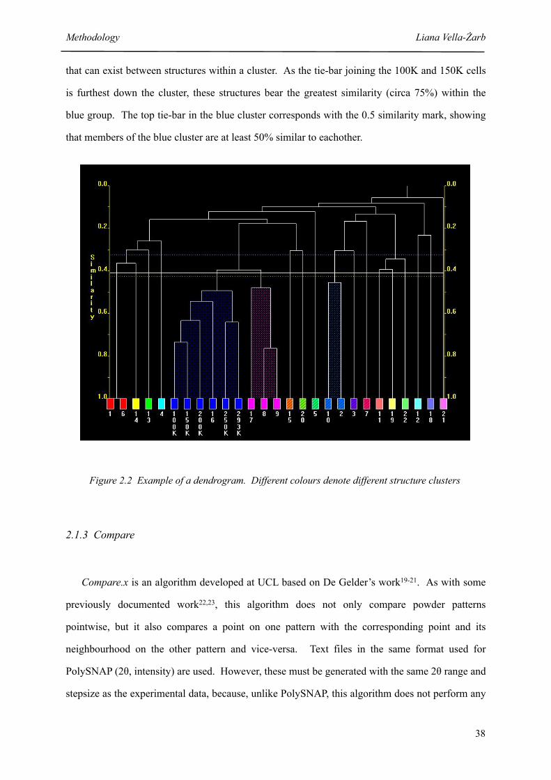
that can exist between structures within a cluster. As the tie-bar joining the 100K and 150K cells
is furthest down the cluster, these structures bear the greatest similarity (circa 75%) within the
blue group. The top tie-bar in the blue cluster corresponds with the 0.5 similarity mark, showing
that members of the blue cluster are at least 50% similar to eachother.
Figure 2.2 Example of a dendrogram. Different colours denote different structure clusters
2.1.3 Compare
Compare.x is an algorithm developed at UCL based on De Gelder’s work19-21. As with some
previously documented work22,23, this algorithm does not only compare powder patterns
pointwise, but it also compares a point on one pattern with the corresponding point and its
neighbourhood on the other pattern and vice-versa. Text files in the same format used for
PolySNAP (2θ, intensity) are used. However, these must be generated with the same 2θ range and
stepsize as the experimental data, because, unlike PolySNAP, this algorithm does not perform any
Methodology Liana Vella-Żarb
38
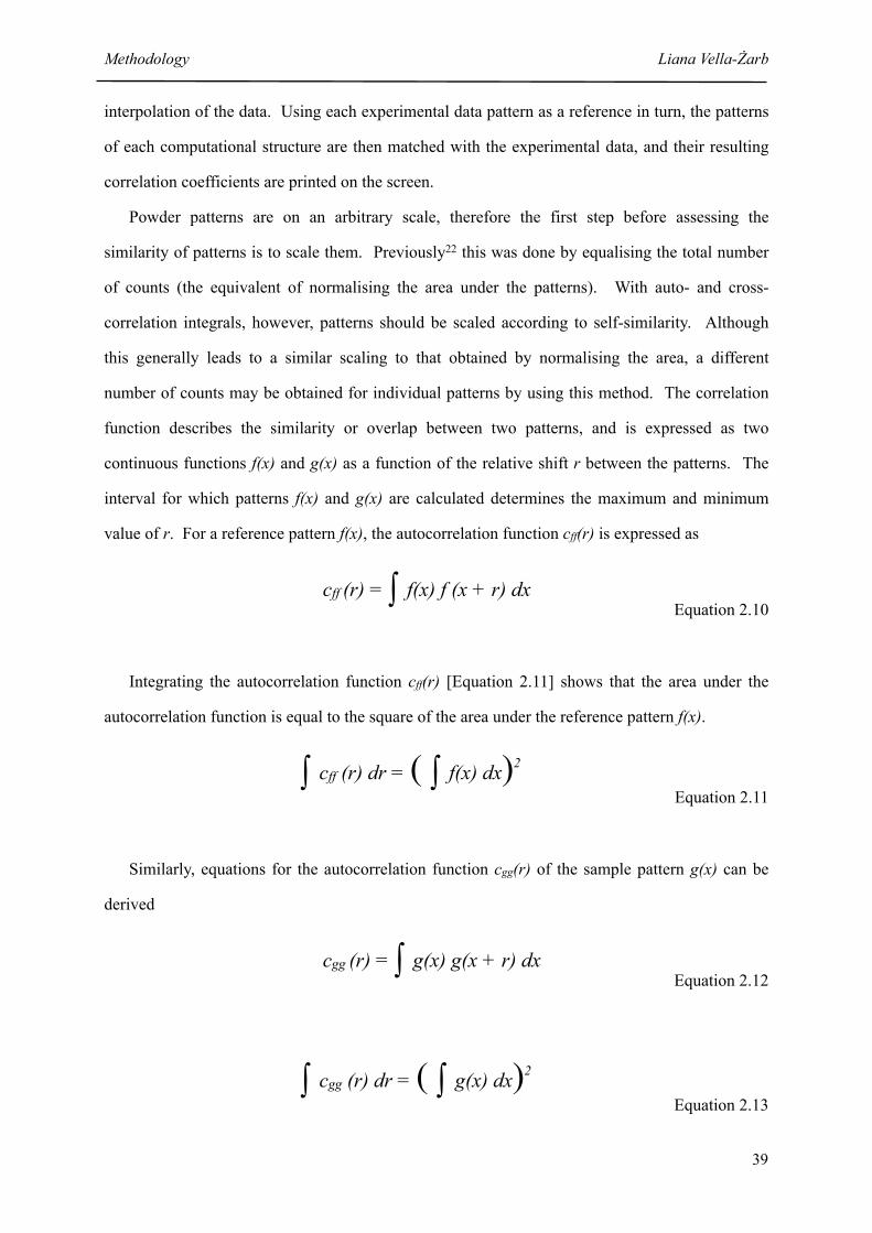
interpolation of the data. Using each experimental data pattern as a reference in turn, the patterns
of each computational structure are then matched with the experimental data, and their resulting
correlation coefficients are printed on the screen.
Powder patterns are on an arbitrary scale, therefore the first step before assessing the
similarity of patterns is to scale them. Previously22 this was done by equalising the total number
of counts (the equivalent of normalising the area under the patterns). With auto- and cross-
correlation integrals, however, patterns should be scaled according to self-similarity. Although
this generally leads to a similar scaling to that obtained by normalising the area, a different
number of counts may be obtained for individual patterns by using this method. The correlation
function describes the similarity or overlap between two patterns, and is expressed as two
continuous functions f(x) and g(x) as a function of the relative shift r between the patterns. The
interval for which patterns f(x) and g(x) are calculated determines the maximum and minimum
value of r. For a reference pattern f(x), the autocorrelation function cff(r) is expressed as
cff (r) = ∫ f(x) f (x + r) dx
Equation 2.10
Integrating the autocorrelation function cff(r) [Equation 2.11] shows that the area under the
autocorrelation function is equal to the square of the area under the reference pattern f(x).
∫ cff (r) dr = ( ∫ f(x) dx)2
Equation 2.11
Similarly, equations for the autocorrelation function cgg(r) of the sample pattern g(x) can be
derived
cgg (r) = ∫ g(x) g(x + r) dx
Equation 2.12
∫ cgg (r) dr = ( ∫ g(x) dx)2
Equation 2.13
Methodology Liana Vella-Żarb
39
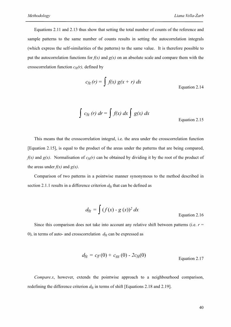
Equations 2.11 and 2.13 thus show that setting the total number of counts of the reference and
sample patterns to the same number of counts results in setting the autocorrelation integrals
(which express the self-similarities of the patterns) to the same value. It is therefore possible to
put the autocorrelation functions for f(x) and g(x) on an absolute scale and compare them with the
crosscorrelation function cfg(r), defined by
cfg (r) = ∫ f(x) g(x + r) dx
Equation 2.14
∫ cfg (r) dr = ∫ f(x) dx ∫ g(x) dx
Equation 2.15
This means that the crosscorrelation integral, i.e. the area under the crosscorrelation function
[Equation 2.15], is equal to the product of the areas under the patterns that are being compared,
f(x) and g(x). Normalisation of cfg(r) can be obtained by dividing it by the root of the product of
the areas under f(x) and g(x).
Comparison of two patterns in a pointwise manner synonymous to the method described in
section 2.1.1 results in a difference criterion dfg that can be defined as
dfg = ∫ ( f (x) - g (x))2 dx
Equation 2.16
Since this comparison does not take into account any relative shift between patterns (i.e. r =
0), in terms of auto- and crosscorrelation dfg can be expressed as
dfg = cff (0) + cgg (0) - 2cfg(0)
Equation 2.17
Compare.x, however, extends the pointwise approach to a neighbourhood comparison,
redefining the difference criterion dfg in terms of shift [Equations 2.18 and 2.19].
Methodology Liana Vella-Żarb
40

dfg = ∫ ( f (x) - g (x + r))2 dx
= cff (0) + cgg (0) - 2cfg(r) Equation 2.18
∫ dfg (r) dr = cff (0) + cgg (0) - 2 ∫ cfg(r) dr Equation 2.19
Using a weighting function w that describes the neighbourhood to be adopted, the similarity
sfg between the two patterns may be expressed either as shown in equation 2.20, or as a function
of dissimilarity [Equation 2.21].
sfg = ∫ wfg (r) cfg (r) dr
( ∫ wff (r) cff (r) dr ∫ wgg (r) cgg (r) dr)½
Equation 2.20
dfg = sff + sgg - 2sfg Equation 2.21
In order to include a neighbourhood in the calculation of similarity or dissimilarity, weighting
functions must be defined for r ≠ 0, and, if they are to be measured on an absolute scale, then wgg
(r), wff (r) and wfg (r) must be equal. The choice of the weighting function wfg (r) depends on the
systems under comparison. For this study, a simple triangle shaped weighting function was used
[Equation 2.22].
wfg (r) = 1- |r| / l if |r| ≺ lwfg (r) = 0 if |r| ≽ l
Equation 2.22
where l defines the width (degrees 2θ) of the neighbourhood taken into account. For this study, a
range of triangle widths (varying from 0.5 to 4 degrees in 2θ, at increments of 0.5) was studied,
with a default value of 2 being decided upon as it was found to give the most consistent results.
Methodology Liana Vella-Żarb
41
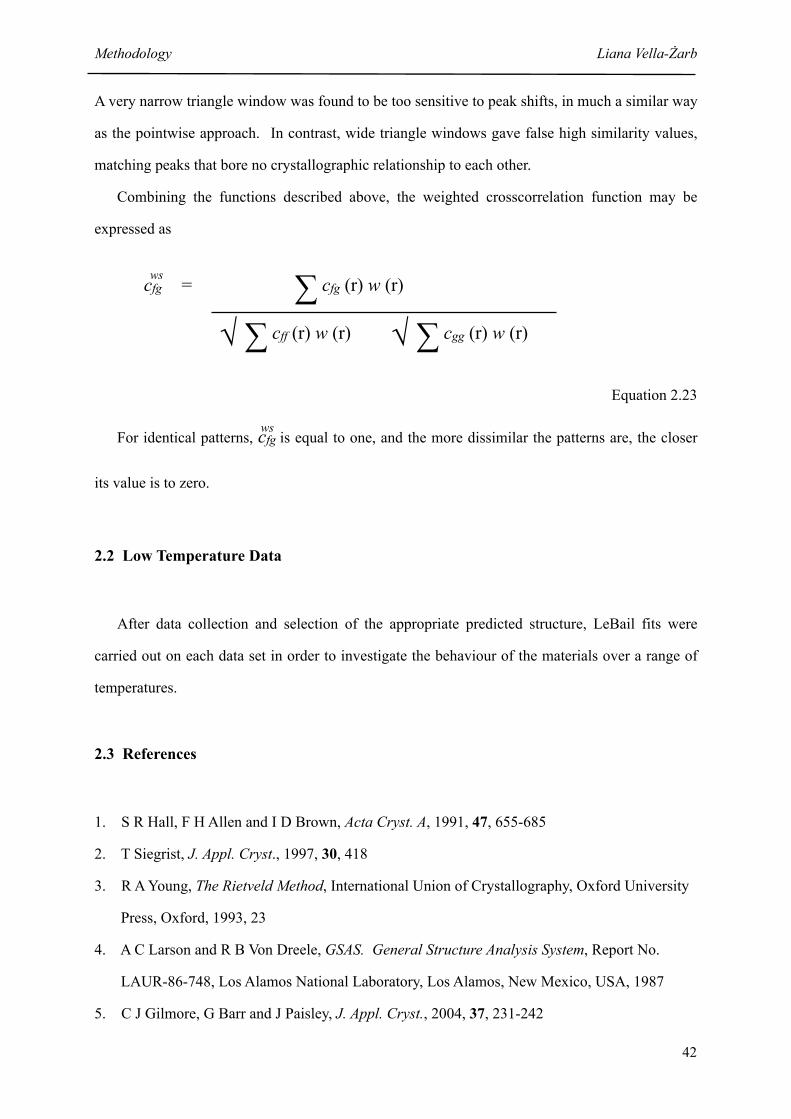
A very narrow triangle window was found to be too sensitive to peak shifts, in much a similar way
as the pointwise approach. In contrast, wide triangle windows gave false high similarity values,
matching peaks that bore no crystallographic relationship to each other.
Combining the functions described above, the weighted crosscorrelation function may be
expressed as
wscfg = ∑ cfg (r) w (r)
√ ∑ cff (r) w (r) √ ∑ cgg (r) w (r)
Equation 2.23
ws
For identical patterns, cfg is equal to one, and the more dissimilar the patterns are, the closer
its value is to zero.
2.2 Low Temperature Data
After data collection and selection of the appropriate predicted structure, LeBail fits were
carried out on each data set in order to investigate the behaviour of the materials over a range of
temperatures.
2.3 References
1. S R Hall, F H Allen and I D Brown, Acta Cryst. A, 1991, 47, 655-685
2. T Siegrist, J. Appl. Cryst., 1997, 30, 418
3. R A Young, The Rietveld Method, International Union of Crystallography, Oxford University
Press, Oxford, 1993, 23
4. A C Larson and R B Von Dreele, GSAS. General Structure Analysis System, Report No.
LAUR-86-748, Los Alamos National Laboratory, Los Alamos, New Mexico, USA, 1987
5. C J Gilmore, G Barr and J Paisley, J. Appl. Cryst., 2004, 37, 231-242
Methodology Liana Vella-Żarb
42

6. G Barr, W Dong and C J Gilmore, J. Appl. Cryst., 2004, 37, 243-252
7. G Barr, W Dong, C J Gilmore and J Faber, J. Appl. Cryst., 2004, 37, 635-642
8. G Barr, W Dong and C J Gilmore, J. Appl. Cryst., 2004, 37, 874-882
9. W H Press, S A Teukolsky, W T Vetterling and B P Flannery, Numerical Recipes in C,
Cambridge University Press, 1992
10. C J Gilmore, Presented at the ICDD Spring Meeting, Newton Square, Pennsylvania, USA,
1998
11. Ĺ Smrčok, M Ďurík and V Jorík, Powder Diffr., 1999, 14, 300-304
12. D L Donoho and I M Johnstone, J. Am. Stat. Assoc., 1995, 90, 1200-1224
13. R T Ogden, Essential Wavelets for Statistical Applications and Data Analysis, Boston:
Birkhäuser, 1997, 144-148
14. A Savitzky and M J E Golay, Anal. Chem., 1964, 36, 1627-1639
15. W I Conover, Practical Nonparametric Statistics, John Wiley, New York, 1971
16. C Spearman, Am. J. Of Psychol., 1904, 15, 72-101
17. N V Smirnov, Bull. Moscow Univ., 2, 3-16
18. J A Nelder and R Mead, Comput. J., 1965, 7, 308-313
19. R de Gelder, R Wehrens and J A Hageman, J. Comp. Chem., 2001, 22 (3), 273-289
20. E L Willighagen, R Wehrens, P Verwer, R de Gelder and L M C Buydens, Acta Cryst. B,
2005, 61, 29-36
21. J A Hageman, R Wehrens, R de Gelder and L M C Buydens, J. Comp. Chem., 2003, 24, 1043-
1051
22. H R Karfunkel, B Rohde, F J J Leusen, R J Gdanitz and G J Rihs, Comp. Chem., 1993, 14,
1125
23. D S Stephenson and G J Binsch, J. Magn. Res., 1980, 37, 409
Methodology Liana Vella-Żarb
43

3. EXPERIMENTAL
3.1 Instrumentation
The following instruments were used for X-ray powder diffraction data collection:
(i) Bruker AXS D5000 high-resolution powder diffractometer.
For each material, the sample was ground using a mortar and pestle and mounted on a flat
disc between two layers of transparent tape, creating a circular area of approximately 1 cm in
diameter. The powder X-Ray diffraction pattern was then recorded in transmission mode using a
position-sensitive detector covering 8o in 2θ, using CuKα1, λ = 1.54056 Å radiation (Ge
monochromated). Data were collected over the range of 5o<2θ<60o, measured in steps of
0.020343o over a total collection time of one hour. Longer runs were carried out using the same
step size over the range of 5o<2θ<60o collected over a period of approximately 14 hours.
(ii) Bruker AXS D5005 high-resolution powder diffractometer.
Samples were ground using a mortar and pestle and placed in the low-temperature sample
holder which consists of a square-shaped recess in a brass container. These data were initially
collected only for 5-azauracil, chlorothalonil and imidazole. The D5005 diffractometer runs in
reflection mode using CuKα1,2 radiation (λ = 1.541838 Å), and is equipped with a Gobel mirror
and a position-sensitive detector covering 8o in 2θ. Data were collected over the range of
5o<2θ<55o, measured in steps of 0.014102o over a total collection time of three hours. Longer
runs were carried out using the same step size over the range of 5o<2θ<55o collected over a period
of approximately 14 hours. The low temperature stage was an Oxford Instruments CCC1101T
stage, protected by three vacuum-sealed shields. Data sets were initially collected over a range of
temperatures (75K, 100K, 125K, 150K, 175K, 200K, 225K, 250K and 293K). However, problems
with transparency prompted the introduction of NaCl into the sample holder. Readings were
repeated at a later date, using a thin layer of the pure material attached to the inverted sample
holder by means of double-sided tape [Figure 3.3]. Data were subsequently collected over a range
of temperatures (10K, 50K, 100K, 150K, 200K, 250K and 293K).
Experimental Liana Vella-Żarb
44

(iii) Bruker AXS D8 high-resolution powder diffractometer.
Low temperature capillary data were collected on this diffractometer in the Department of
Chemistry at the University of Glasgow following observation of preferred orientation in the
diffraction patterns obtained with the D5005. The samples were ground using a mortar and pestle
and packed into 0.5mm glass capillary tubes to a depth of approximately 3cm. All tubes had their
ends sealed before being mounted onto the capillary stage, which was then set to rotate. The
powder X-ray diffraction patterns were recorded in transmission mode using a position sensitive
detector covering 8o in 2θ, using Ge monochromated CuKα1 radiation (λ = 1.54056 Å). Data were
collected over the range of 5o<2θ<55o, measured in steps of 0.014102o over a total collection time
of three hours, at various temperatures (70K, 100K, 150K, 200K, 250K and 293K) using a
cryostream. Liquid nitrogen is drawn up by the action of the diaphragm pump from an
unpressurised supply vessel into the cryostream coldhead, where it then passes through a heater
so that most of the liquid is turned into vapour at the boiling point of liquid nitrogen. This vapour
is then dried with a line drier unit to ensure there is no moisture in the gas. The flow rate of the
gas from the pump is regulated by a variable flow controller as the gas flows back into the
cryostream coldhead where it is recooled. A heater and a sensor regulate the temperature of the
vapour before it enters the nozzle of the cryostream. The gas then flows along the isothermal
nozzle and out over the sample.
3.2 Sample Effects
Powder data for all samples were collected on the D5000 at room temperature. Low
temperature data collection was initially carried out on the D5005 with its original sample cell set-
up. Transparency and sample contraction issues then prompted the use of an internal inorganic
standard, NaCl, introduced into the sample in the ratio 1:2. However, analysis of the resulting
powder patterns and problems with Rietveld refinement revealed a substantial degree of preferred
orientation in some of the samples, thus inspiring the use of a capillary set-up rather than a flat
sample holder in cases where preferred orientation was observed.
Experimental Liana Vella-Żarb
45
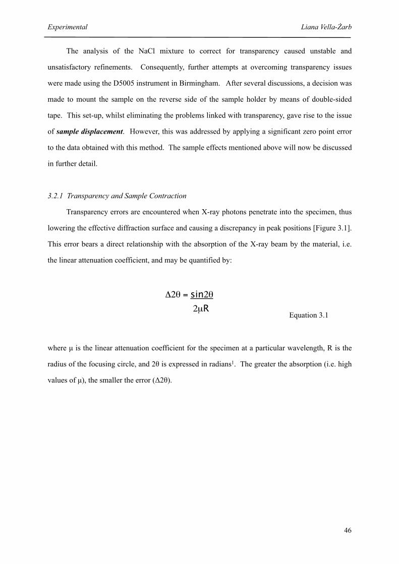
The analysis of the NaCl mixture to correct for transparency caused unstable and
unsatisfactory refinements. Consequently, further attempts at overcoming transparency issues
were made using the D5005 instrument in Birmingham. After several discussions, a decision was
made to mount the sample on the reverse side of the sample holder by means of double-sided
tape. This set-up, whilst eliminating the problems linked with transparency, gave rise to the issue
of sample displacement. However, this was addressed by applying a significant zero point error
to the data obtained with this method. The sample effects mentioned above will now be discussed
in further detail.
3.2.1 Transparency and Sample Contraction
Transparency errors are encountered when X-ray photons penetrate into the specimen, thus
lowering the effective diffraction surface and causing a discrepancy in peak positions [Figure 3.1].
This error bears a direct relationship with the absorption of the X-ray beam by the material, i.e.
the linear attenuation coefficient, and may be quantified by:
Δ2θ = sin2θ
2µR Equation 3.1
where µ is the linear attenuation coefficient for the specimen at a particular wavelength, R is the
radius of the focusing circle, and 2θ is expressed in radians1. The greater the absorption (i.e. high
values of µ), the smaller the error (Δ2θ).
Experimental Liana Vella-Żarb
46
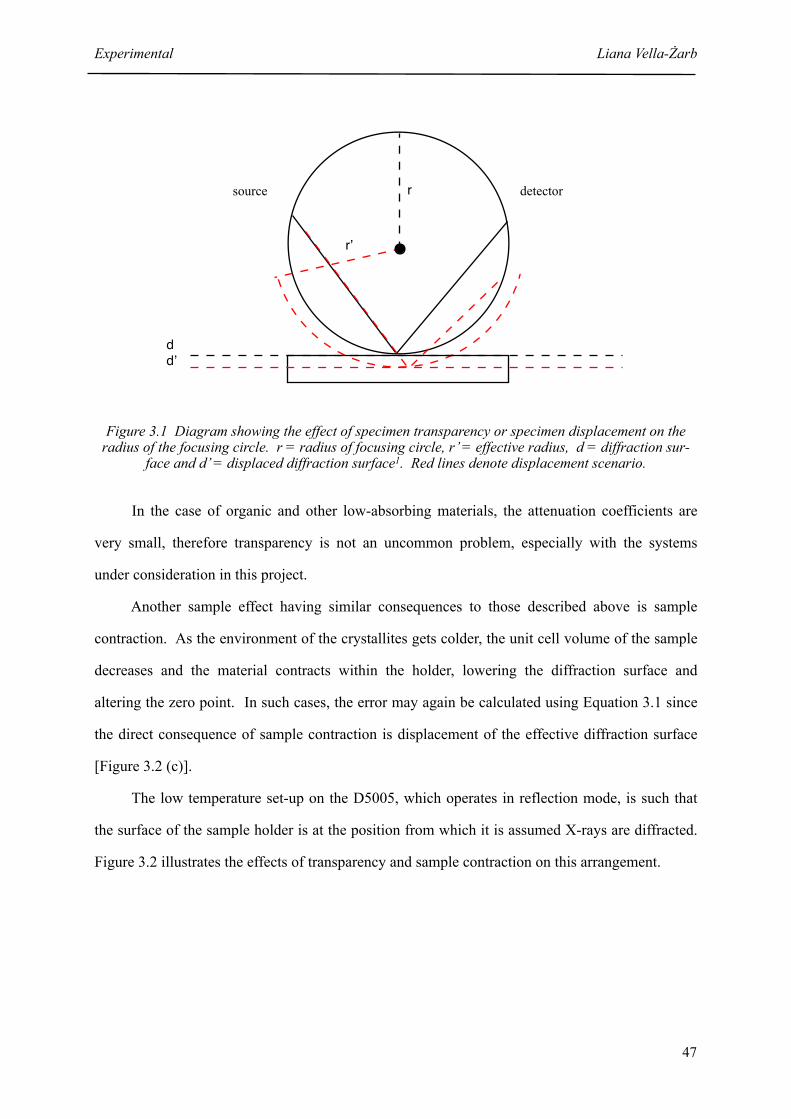
ddʼ
r
rʼ
source detector
Figure 3.1 Diagram showing the effect of specimen transparency or specimen displacement on the radius of the focusing circle. r = radius of focusing circle, r’ = effective radius, d = diffraction sur-
face and d’ = displaced diffraction surface1. Red lines denote displacement scenario.
In the case of organic and other low-absorbing materials, the attenuation coefficients are
very small, therefore transparency is not an uncommon problem, especially with the systems
under consideration in this project.
Another sample effect having similar consequences to those described above is sample
contraction. As the environment of the crystallites gets colder, the unit cell volume of the sample
decreases and the material contracts within the holder, lowering the diffraction surface and
altering the zero point. In such cases, the error may again be calculated using Equation 3.1 since
the direct consequence of sample contraction is displacement of the effective diffraction surface
[Figure 3.2 (c)].
The low temperature set-up on the D5005, which operates in reflection mode, is such that
the surface of the sample holder is at the position from which it is assumed X-rays are diffracted.
Figure 3.2 illustrates the effects of transparency and sample contraction on this arrangement.
Experimental Liana Vella-Żarb
47
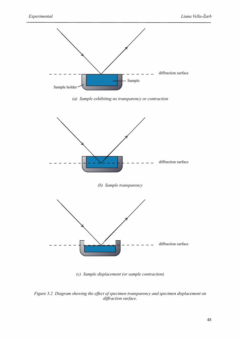
diffraction surface
Sample holderSample
(a) Sample exhibiting no transparency or contraction
diffraction surface
(b) Sample transparency
diffraction surface
(c) Sample displacement (or sample contraction)
Figure 3.2 Diagram showing the effect of specimen transparency and specimen displacement on diffraction surface.
Experimental Liana Vella-Żarb
48

To monitor the effects of sample transparency, an inorganic material not prone to
transparency effects was added to the sample. NaCl was selected as its lattice parameters and
behaviour over a range of low temperatures are well-documented2, and it is unreactive with the
materials of relevance to this project. For more accurate LeBail analysis, the cell parameters for
NaCl must take thermal contraction into account. A thermal expansion coefficient was therefore
applied to the NaCl structure, and peak positions calculated for the salt peaks over the range of
temperatures studied [Table 3.1].
Table 3.1. Calculated peaks for NaCl with a change in temperature at different wavelengths (*Coefficient of thermal expansion for NaCl = -40.5 × 10⁻⁶ Å/K)2
Temperature Corrected a Cu-Kα Cu-Kα1
(K) (Å) Peak 1
Peak 2
Peak 3
Peak 1
Peak 2
Peak 3
250 5.6385 27.397 31.739 45.500 27.374 31.712 45.461
225 5.6375 27.402 31.745 45.509 27.379 31.718 45.469
200 5.6365 27.407 31.751 45.517 27.384 31.724 45.478
175 5.6355 27.412 31.756 45.526 27.389 31.730 45.486
150 5.6345 27.417 31.762 45.535 27.394 31.735 45.495
125 5.6335 27.422 31.768 45.543 27.399 31.741 45.503
100 5.6324 27.427 31.774 45.552 27.404 31.747 45.513
75 5.6314 27.432 31.780 45.561 27.409 31.753 45.521
3.2.2 Sample Displacement
A more efficient method of data collection which avoids sample transparency and reduces
contraction errors involves mounting a fine layer of the sample on the reverse side of the sample
holder using double-sided tape. By this method, the sample height is slightly displaced from its
original position, thus causing a zero point error [Figure 3.3]. This error is constant and can
therefore be calculated prior to the refinement stage [Equation 3.1].
Experimental Liana Vella-Żarb
49

sample
diffracting surface
(a) Traditional technique
displaced diffracting surface
sample
double-sided tape
(a) Modified technique
Figure 3.3 Diagram showing the techniques used to mount the sample onto the sample holder for collection of low-temperature data on the D5005.
3.2.3 Preferred Orientation
In an ideal powder sample, the crystallites are oriented completely randomly and
independently from the direction of the beam. This gives each crystal orientation the same
probability of reaching the diffraction condition. Preferred orientation is a property arising when
the crystallites in a sample have a stronger tendency to be oriented in one way rather than another.
For sample identification and fingerprinting purposes, preferred orientation is often not
critical as it does not affect the positions of the peaks observed. It does, however, affect the
relative peak intensities within a pattern, thus hindering reliable intensity extraction and
consequently structure solution and refinement. The type and extent of preferred orientation is
often dependent on the crystal habit of the material. Anisotropic crystallites, eg. long needles or
flat platelets, tend to exhibit preferred orientation and pack preferentially in certain directions
rather that others.
When a material is packed into a flat sample holder (and sometimes backed with a glass
slide), as in the case of the D5005 low temperature original set-up, preferred orientation of the
crystallites can sometimes be encouraged. The cleavage (or growth faces) of the material, which
are all of the same crystallographic type, align themselves mostly parallel to the direction of the
packing, with only a small proportion perpendicular to the surface. The direction that lies
Experimental Liana Vella-Żarb
50

perpendicular to the flat sides of the surfaces is the preferred orientation axis, and the intensities
of reflections from planes perpendicular to this axis will be enhanced, while those from the
parallel planes will be suppressed.
Since preferred orientation produces systematic distortions of the reflection intensities,
mathematical models can be used to correct for this effect during refinement. However, this is not
so reliable in cases of structure solution. It is believed that few powder patterns are completely
free from this phenomenon3, and it has consequently become routine practice to incorporate
corrections for preferred orientation in Rietveld refinement processes.
Attempts at forcing a material to take up random orientation may often prove futile, as
preferred orientation is a problem that, if present, can generally be reduced but not eliminated
completely by experimental measures. Care when preparing and mounting the sample is
important in avoiding this bias, as excess compression or sliding the backing glass can encourage
the alignment of anisotropic crystallites. Consequently, the use of capillaries rather than flat
sample holders may sometimes address this issue. Other experimental techniques which may be
employed to mimic the random orientation of more isotropic materials include mixing the sample
with an amorphous material, spray-drying and grinding.
3.2.4 Sample Loss
Additional problems were encountered through sample loss during initial data collection on
the D5005. The design of the low-temperature apparatus is such that a high vacuum is created
around the specimen chamber, to allow such extreme temperatures to be reached. Any gaps
arising between these chambers cause a pressure difference that may lead to a change in
orientation of the powder particles, or (as in the case of imidazole) to some of the more volatile
samples being vacuumed out of the sample holder. The consequences are similar to those
observed with transparency and sample displacement. In the case of the D5005, use of the reverse
side of the sample holder avoided this problem.
Experimental Liana Vella-Żarb
51

3.3 Materials
With the exception of the data collected on the D5005 using the internal standard, all
samples were used in their original form, as received from the supplier or originator. The
following table illustrates the materials used and the data sets collected at various settings.
Table 3.2 List of data sets collected for each material studied.
D5000 D5005(original)
D5005(mixed with
salt)
D8(capillary)
D5005(thin film on reverse side)
Adenine
5-Azauracil
Chlorothalonil
Guanine
Imidazole
✓ ✓ ✓
✓ ✓ ✓ ✓
✓ ✓ ✓ ✓ ✓
✓ ✓
✓ ✓ ✓ ✓ ✓
3.4 References
1. R Jenkins and R L Snyder, Introduction to X-Ray Powder Diffractometry, Wiley Interscience,
New York, 1996.
2. P D Pathak and N G Vasavada, Acta Cryst. A, 1970, 26, 655
3. E Sturm and W Lodding, Acta Cryst. A, 1968, 24, 650
Experimental Liana Vella-Żarb
52

4. IMIDAZOLE
4.1 Background
The simplest member of the imidazole family is imidazole itself: a colourless to pale yellow
crystalline solid with a weak amine-like odour. Whilst being generally poorly soluble in water, its
derivatives dissolve in organic solvents such as chloroform, propylene glycol and polyethoxylated
castor oil. They are antimetabolites and inhibitors of histamine, and are commonly used as
insecticides.
The imidazole molecule has a high propensity for side-chain substitution, and the composition
of such chains is accountable for the activity of the material, as well as its degree of toxicity.
Thus, imidazole compounds have various commercial uses, ranging from topical antimycotics
(e.g. clotrimazole, miconazole and ketoconazole)1 to industrial fungicides (e.g. imazalil). Some
also exhibit antibacterial, antiprotozoal and antihelmintic activity (e.g. metronidazole, tinidazole
and mebendazole respectively)1. Imidazole and its derivatives are also widely used as
intermediates in the synthesis of organic compounds including pharmaceuticals, agrochemicals,
dyes, photographic chemicals, corrosion inhibitors, epoxy curing agents, adhesives and plastic
modifiers.
Imidazole Liana Vella-Żarb
53
Figure 4.1. Imidazole (1,3-diaza-2,4-cyclopentadiene)
N
N HH
HH

4.1.1 Crystal Structure
The crystal structure of imidazole was determined by single crystal neutron diffraction at
103K, with additional studies carried out at 108K, 113K, 123K and 293K 2 [Table 4.1].
Imidazole has a monoclinic (P21/c) lattice, with Z = 4, and has not yet been shown to exhibit
polymorphic behaviour. It has polar hydrogen atoms that form hydrogen bonds to the lone pairs
on the nitrogen atom. These form twisted chains that run parallel to the c axis [Figures 4.2 and
4.3].
Figure 4.2. Imidazole molecules forming chains parallel to the c axis. Dotted lines denote NH...N hydrogen bonds
Adjacent molecules in the chains are twisted by about 60o with respect to each other, and these
chains are joined by short N-H….N contacts (H......Acceptor distance of 1.8085Å). The hydrogen
bonds, forming a network through the crystal, result in dominant electrostatic interactions, giving
an estimated electrostatic contribution of about 60% of the total lattice energy3.
Imidazole Liana Vella-Żarb
54

Figure 4.3. A view down the c axis
4.1.2 Crystal Structure Prediction
Imidazole represents an “ideal” system for structure prediction studies4, given that it is a rigid
structure. This means that the frequencies of the low energy k=0 (where k is the kinetic energy)
intermolecular lattice vibrations obtained by lattice energy minimisation are a close representation
of the experimental system4. At a temperature of 0 K, the system is thermodynamically most
stable. The computational search resulted in a total of 65 theoretical structures for imidazole,
many of which vary only slightly in density, and lie within 7 kJ mol-1 of the global minimum4
[Figure 4.4].
Imidazole Liana Vella-Żarb
55

Total Lattice Energy vs Cell Density
-76
-75
-74
-73
-72
-71
-70
-691.14 1.16 1.18 1.2 1.22 1.24 1.26 1.28 1.3 1.32
Cell Density per molecule
Tota
l Lat
tice
Ener
gy
C 1 2 1C 1 2/c 1C 1 c 1P 1P -1P 1 21 1P 1 21/c 1P 1 21/n 1P 21 21 21P b c aP c a 21P n a 21Experimental form
Figure 4.4 The distribution of low energy structures found in the search for minima in the lattice energy of imidazole. The minimum corresponding to the known crystal structure (ExpMinOpt) is
denoted by the open red diamond4. [Permission for reproduction granted by the author of reference 4.]
Variations from the known crystal structure are observed on comparison of the low energy
structures, and although the structures are very similar, comparison of the powder patterns reveals
their differences. Although the global minimum corresponds to the known crystal structure, there
are structures within 2 kJ mol-1 in which the hydrogen-bonded molecules are coplanar, and others
lying within 3.5 kJ mol-1 which differ in the arrangement of the hydrogen-bonded chains.
However, all the low energy crystal structures are based on the same hydrogen bonding network
and they favour the anti-parallel stacking of chains4.
The experimental and ab initio optimised molecular structures exhibit only minor differences,
and the most thermodynamically stable predicted structure at 0K corresponds with the known
crystal structure4. Although other structures are thermodynamically feasible, the same hydrogen
bonding motif is dominant, thus making manipulation of crystallisation conditions unlikely to
give a kinetic advantage in the nucleation and growth of a long-lived polymorph.
Imidazole Liana Vella-Żarb
56
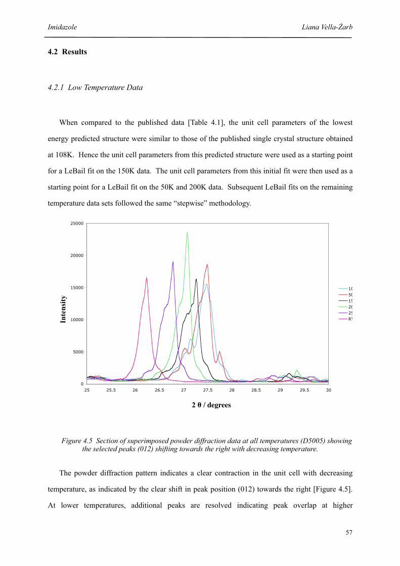
4.2 Results
4.2.1 Low Temperature Data
When compared to the published data [Table 4.1], the unit cell parameters of the lowest
energy predicted structure were similar to those of the published single crystal structure obtained
at 108K. Hence the unit cell parameters from this predicted structure were used as a starting point
for a LeBail fit on the 150K data. The unit cell parameters from this initial fit were then used as a
starting point for a LeBail fit on the 50K and 200K data. Subsequent LeBail fits on the remaining
temperature data sets followed the same “stepwise” methodology.
0
5000
10000
15000
20000
25000
25 25.5 26 26.5 27 27.5 28 28.5 29 29.5 30
10K50K150K200K250KRT
2 θ / degrees
Inte
nsity
Figure 4.5 Section of superimposed powder diffraction data at all temperatures (D5005) showing the selected peaks (012) shifting towards the right with decreasing temperature.
The powder diffraction pattern indicates a clear contraction in the unit cell with decreasing
temperature, as indicated by the clear shift in peak position (012) towards the right [Figure 4.5].
At lower temperatures, additional peaks are resolved indicating peak overlap at higher
Imidazole Liana Vella-Żarb
57

temperatures. This overlap is reduced as the structure contracts anisotropically, thus exhibiting a
difference in shift between peaks representing distinct reflections. The effect of changing
temperature over the entire diffraction pattern from 10 to 45 degrees along 2θ is shown in
Appendix A2.1.
The percentage differences in a, b, c, β and volume with varying temperature were calculated
and, as expected, the volume increases as higher temperatures are reached, while a, b, c and β
change accordingly to accomodate this expansion [Table 4.1 and Figure 4.6].
Table 4.1 Unit cell parameters of lowest energy predicted structure and determined from experimental data, and published unit cell dimensions for imidazole with changing temperature. The numbers in brackets denote the percentage change with respect to those values obtained from the 10K data.
Temperature (K) a (Å) b (Å) c (Å) β(o) Volume (Å3)
Single Crystal Values2
103 7.569 (1) 5.366 (1) 9.785 (2) 119.08 (1) 347.32
108 7.572 (2) 5.368 (1) 9.782 (2) 119.03 (1) 347.65
113 7.577 (2) 5.373 (1) 9.777 (3) 118.93 (2) 348.36
123 7.583 (1) 5.375 (1) 9.779 (2) 118.92 (1) 348.87
Predicted values4 (0K) 7.57 5.37 9.78 119.1 347.3
10 7.537 (1)(0.00)
5.078 (2)(0.00)
9.410 (1)(0.00)
120.83 (2)(0.00)
309.26(0.00)
50(% change)
7.476 (1)(-0.81)
5.238 (3)(+3.14)
9.571 (2)(+1.72)
119.55 (3)(-1.06)
326.06(+5.43)
150(% change)
7.561 (2)(+0.31)
5.335 (2)(+5.06)
9.762 (1)(+3.74)
120.09 (1)(-0.61)
340.71(+10.17)
200(% change)
7.612 (1)(+0.99)
5.349 (3)(+5.34)
9.823 (1)(+4.39)
118.60 (1)(-1.85)
351.17(+13.55)
250(% change)
7.749 (3)(+2.82)
5.358 (2)(+5.51)
9.712 (2)(+3.22)
119.15 (3)(-1.39)
352.22(+13.89)
293(% change)
7.742 (2)(+2.73)
5.382 (3)(+5.97)
9.646 (1)(+2.51)
117.76 (1)(-2.54)
355.67(+15.01)
293 (D5000) 7.569 (1)(+0.43)
5.366 (1)(+5.66)
9.779 (2)(+3.93)
119.10 (1)(-1.43)
347.04(+12.23)
Imidazole Liana Vella-Żarb
58

-4
-2
0
2
4
6
8
10
12
14
16
10 50 150 200 250 293
a
b
c
Beta
Vol
% c
hang
e
Temperature (K)
Figure 4.6 Graph showing the percentage change in unit cell dimensions with temperature.
Over the range of temperatures, the unit cell volume would be expected to increase as a
result of thermal expansion. In the case of imidazole, a and b were found to increase overall with
temperature, while c and β showed irregular behaviour. Although atypical, these changes in the
lattice parameters still resulted in an overall expansion of the unit cell, as indicated by the increase
in volume. This anisotropic behaviour will be due to relative hydrogen bond strengths and sterics
in each direction. However, the LeBail fits used here may show a significant correlation of lattice
parameters during fitting, making these results unreliable. Hence these results will not be
interpreted further in this work.
Imidazole Liana Vella-Żarb
59

4.2.2 Automated Comparison
4.2.2.1 Rwp
The 65 predicted structures were each compared, using Rwp, with the experimental data
collected at each temperature. The outcome of these comparisons was non-discriminatory, with
none of the 65 structures singled out as being significantly similar to any of the experimental data.
Rwp values ranging from 51.83% to 79.94% were obtained, although in most cases, no significant
discrimination was found [Table 4.2, Figures 4.7 and 4.8]. In addition, only one of the predictions
(ai35) was ranked as the best fit to data recorded at two different temperatures. The correct
predicted structure (ak34) was not identified by Rwp as having a similar powder pattern to the data
collected at any of the temperatures. The simulated patterns for all predicted structures shown in
the table and the corresponding experimental patterns are found in Appendix A2.2.
Table 4.2. Structures with lowest Rwp identified at each temperature. The difference is that between the Rwp for the top ranked structure [Rwp(x)] and the correct prediction [Rwp(ak34)] at each temperature. Black numbers denote the correct structure being ranked top, while red numbers denote incorrect structures ranked as the best.
Temperature (K) Top ranked
structure
Rwp (x) (%) Rwp (ak34) (%) Difference (%)[Rwp(x) - Rwp(ak34)]
10
50
150
200
250
293
293 (D5000)
ca61 66.5 71.5 -5.0
ca34 66.5 68.5 -2.0
ai35 52.9 67.6 -14.7
de38 51.8 72.2 -20.4
ai35 59.3 65.0 -5.7
am36 56.5 59.9 -3.4
am44 70.7 71.7 -1.0
Imidazole Liana Vella-Żarb
60

Figure 4.7 Rwp values for each predicted structure at each temperature. The arrow indicates structure ak34.
Rwp (%)
aa12ab14af57
ah115ah35ah4
ah45ah46ah59ah60ah63ah8
ah95ai35ai46
ak34ak61ak66ak97
am108am124am20am32am36am41am43am44am63am77aq115aq123aq13aq6
av47av6
ay112ay121ay24ay89az68bd19bd37bd71ca34ca61cb42cb97cc11cc35da16da33da36da38da4
da71db31db75dc40dc79dd71
de102de38de45fa46fc72
Str
uct
ure
Figure X.7 Rwp values for each predicted structure at each temperature. The arrow indicates structure ak34.
aa12ab14af57ah115ah35ah4ah45ah46ah59ah60ah63ah8ah95ai35ai46ak34ak61ak66ak97am108am124am20am32am36am41am43am44am63am77aq115aq123aq13aq6av47av6
ay112ay121ay24ay89az68bd19bd37bd71ca34ca61cb42cb97cc11cc35da16
da33da36da38da4da71db31db75dc40dc79dd71de102de38de45fa46fc72
Correlation
Structure
Imidazole Liana Vella-Żarb
61

aa12ab14af57
ah115ah35ah4
ah45ah46ah59ah60ah63ah8
ah95ai35ai46
ak34ak61ak66ak97
am108am124am20am32am36am41am43am44am63am77aq115aq123aq13aq6
av47av6
ay112ay121ay24ay89az68bd19bd37bd71ca34ca61cb42cb97cc11cc35da16da33da36da38da4
da71db31db75dc40dc79dd71
de102de38de45fa46fc72
Rwp (%)
Stru
ctur
e
Figure 4.8 Rwp values for each predicted structure against the D5000 data at room temperature. The arrow indicates the correct structure ak34.
Imidazole Liana Vella-Żarb
62

4.2.2.2 PolySNAP
Figure 4.9. Dendrogram showing similarity clusters for imidazole predicted and experimental powder patterns
For PolySNAP analysis, the data collected on the different diffractometers were analysed
separately due to the difference in wavelength between the two setups. In the dendrogram
comparing all 65 predicted structures with the D5005 data [Figure 4.9], structure ak34, which
corresponds to the published structure, was grouped with the entire set of experimental data at all
temperatures (cluster marked in red). Although all experimental data were grouped together, it
was interesting to note that within this cluster were paired subsets, with the lower temperature
data pair being ranked as more similar to each other than the next pair up. Taking each
temperature separately and looking at the structure with the highest correlation in each case,
structure ak34 was the top ranking structure at all temperatures above 150K [Table 4.3].
Imidazole Liana Vella-Żarb
63
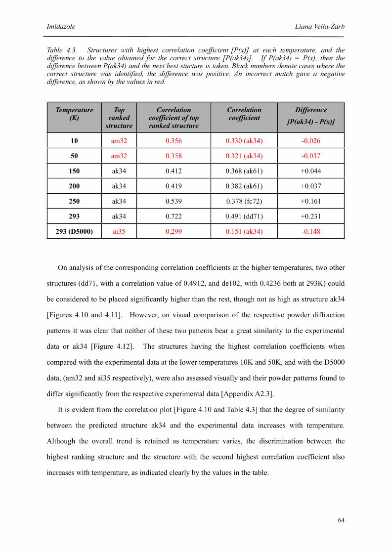
Table 4.3. Structures with highest correlation coefficient [P(x)] at each temperature, and the difference to the value obtained for the correct structure [P(ak34)]. If P(ak34) = P(x), then the difference between P(ak34) and the next best stucture is taken. Black numbers denote cases where the correct structure was identified, the difference was positive. An incorrect match gave a negative difference, as shown by the values in red.
Temperature (K)
Top ranked
structure
Correlation coefficient of top ranked structure
Correlation coefficient
Difference[P(ak34) - P(x)]
10
50
150
200
250
293
293 (D5000)
am32 0.356 0.330 (ak34) -0.026
am32 0.358 0.321 (ak34) -0.037
ak34 0.412 0.368 (ak61) +0.044
ak34 0.419 0.382 (ak61) +0.037
ak34 0.539 0.378 (fc72) +0.161
ak34 0.722 0.491 (dd71) +0.231
ai35 0.299 0.151 (ak34) -0.148
On analysis of the corresponding correlation coefficients at the higher temperatures, two other
structures (dd71, with a correlation value of 0.4912, and de102, with 0.4236 both at 293K) could
be considered to be placed significantly higher than the rest, though not as high as structure ak34
[Figures 4.10 and 4.11]. However, on visual comparison of the respective powder diffraction
patterns it was clear that neither of these two patterns bear a great similarity to the experimental
data or ak34 [Figure 4.12]. The structures having the highest correlation coefficients when
compared with the experimental data at the lower temperatures 10K and 50K, and with the D5000
data, (am32 and ai35 respectively), were also assessed visually and their powder patterns found to
differ significantly from the respective experimental data [Appendix A2.3].
It is evident from the correlation plot [Figure 4.10 and Table 4.3] that the degree of similarity
between the predicted structure ak34 and the experimental data increases with temperature.
Although the overall trend is retained as temperature varies, the discrimination between the
highest ranking structure and the structure with the second highest correlation coefficient also
increases with temperature, as indicated clearly by the values in the table.
Imidazole Liana Vella-Żarb
64

Correlation
Stru
ctur
e
Figure 4.10 Correlation coefficients of all 65 structures at each temperature. The arrow indicates structure ak34
Imidazole Liana Vella-Żarb
65

aa12ab14af57
ah115ah35ah4
ah45ah46ah59ah60ah63ah8
ah95ai35ai46
ak34ak61ak66ak97
am108am124am20am32am36am41am43am44am63am77aq115aq123aq13aq6
av47av6
ay112ay121ay24ay89az68bd19bd37bd71ca34ca61cb42cb97cc11cc35da16da33da36da38da4
da71db31db75dc40dc79dd71
de102de38de45fa46fc72
Correlation
Stru
ctur
e
Figure 4.11 Correlation coefficients of all 65 structures against the D5000 data. The arrow indicates structure ak34
Imidazole Liana Vella-Żarb
66

Intensity
2 θ
/ deg
rees
Figure 4.12 Powder diffraction patterns for five selected predicted structures and the experimental structure at room temperature (D5005).
Imidazole Liana Vella-Żarb
67
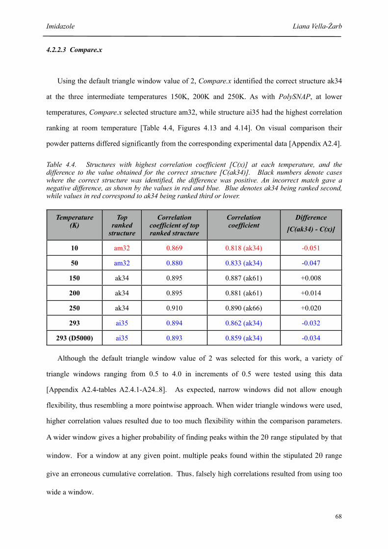
4.2.2.3 Compare.x
Using the default triangle window value of 2, Compare.x identified the correct structure ak34
at the three intermediate temperatures 150K, 200K and 250K. As with PolySNAP, at lower
temperatures, Compare.x selected structure am32, while structure ai35 had the highest correlation
ranking at room temperature [Table 4.4, Figures 4.13 and 4.14]. On visual comparison their
powder patterns differed significantly from the corresponding experimental data [Appendix A2.4].
Table 4.4. Structures with highest correlation coefficient [C(x)] at each temperature, and the difference to the value obtained for the correct structure [C(ak34)]. Black numbers denote cases where the correct structure was identified, the difference was positive. An incorrect match gave a negative difference, as shown by the values in red and blue. Blue denotes ak34 being ranked second, while values in red correspond to ak34 being ranked third or lower.
Temperature (K)
Top ranked
structure
Correlation coefficient of top ranked structure
Correlation coefficient
Difference[C(ak34) - C(x)]
10
50
150
200
250
293
293 (D5000)
am32 0.869 0.818 (ak34) -0.051
am32 0.880 0.833 (ak34) -0.047
ak34 0.895 0.887 (ak61) +0.008
ak34 0.895 0.881 (ak61) +0.014
ak34 0.910 0.890 (ak66) +0.020
ai35 0.894 0.862 (ak34) -0.032
ai35 0.893 0.859 (ak34) -0.034
Although the default triangle window value of 2 was selected for this work, a variety of
triangle windows ranging from 0.5 to 4.0 in increments of 0.5 were tested using this data
[Appendix A2.4-tables A2.4.1-A24..8]. As expected, narrow windows did not allow enough
flexibility, thus resembling a more pointwise approach. When wider triangle windows were used,
higher correlation values resulted due to too much flexibility within the comparison parameters.
A wider window gives a higher probability of finding peaks within the 2θ range stipulated by that
window. For a window at any given point, multiple peaks found within the stipulated 2θ range
give an erroneous cumulative correlation. Thus, falsely high correlations resulted from using too
wide a window.
Imidazole Liana Vella-Żarb
68

Correlation
Stru
ctur
e
aa12ab14af57
ah115ah35ah4
ah45ah46ah59ah60ah63ah8
ah95ai35ai46
ak34ak61ak66ak97
am108am124am20am32am36am41am43am44am63am77aq115aq123aq13aq6
av47av6
ay112ay121ay24ay89az68bd19bd37bd71ca34ca61cb42cb97cc11cc35da16da33da36da38da4
da71db31db75dc40dc79dd71
de102de38de45fa46fc72
Figure 4.13 Correlation coefficients of all 65 structures at each temperature (D5005). The arrow indicates structure ak34.
Imidazole Liana Vella-Żarb
69

Correlation
Stru
ctur
e
aa12ab14af57
ah115ah35ah4
ah45ah46ah59ah60ah63ah8
ah95ai35ai46
ak34ak61ak66ak97
am108am124am20am32am36am41am43am44am63am77aq115aq123aq13aq6
av47av6
ay112ay121ay24ay89az68bd19bd37bd71ca34ca61cb42cb97cc11cc35da16da33da36da38da4
da71db31db75dc40dc79dd71
de102de38de45fa46fc72
Figure 4.14 Correlation coefficients of all 65 structures against the D5000 data. The arrow indicates structure ak34.
Imidazole Liana Vella-Żarb
70
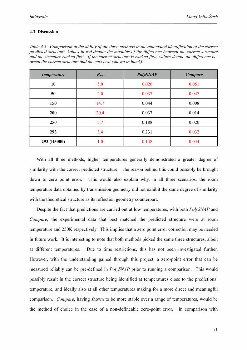
4.3 Discussion
Table 4.5. Comparison of the ability of the three methods in the automated identification of the correct predicted structure. Values in red denote the modulus of the difference between the correct structure and the structure ranked first. If the correct structure is ranked first, values denote the difference be-tween the correct structure and the next best (shown in black).
Temperature Rwp PolySNAP Compare
10 5.0 0.026 0.051
50 2.0 0.037 0.047
150 14.7 0.044 0.008
200 20.4 0.037 0.014
250 5.7 0.188 0.020
293 3.4 0.231 0.032
293 (D5000) 1.0 0.148 0.034
With all three methods, higher temperatures generally demonstrated a greater degree of
similarity with the correct predicted structure. The reason behind this could possibly be brought
down to zero point error. This would also explain why, in all three scenarios, the room
temperature data obtained by transmission geometry did not exhibit the same degree of similarity
with the theoretical structure as its reflection geometry counterpart.
Despite the fact that predictions are carried out at low temperatures, with both PolySNAP and
Compare, the experimental data that best matched the predicted structure were at room
temperature and 250K respectively. This implies that a zero point error correction may be needed
in future work. It is interesting to note that both methods picked the same three structures, albeit
at different temperatures. Due to time restrictions, this has not been investigated further.
However, with the understanding gained through this project, a zero-point error that can be
measured reliably can be pre-defined in PolySNAP prior to running a comparison. This would
possibly result in the correct structure being identified at temperatures close to the predictions’
temperature, and ideally also at all other temperatures making for a more direct and meaningful
comparison. Compare, having shown to be more stable over a range of temperatures, would be
the method of choice in the case of a non-defineable zero-point error. In comparison with
Imidazole Liana Vella-Żarb
71

PolySNAP, Compare gave higher overall correlation coefficients. However, although the
discrimination between the highest ranking structure and the structure with the second highest
correlation coefficient increased with temperature there was less discrimination between the data
when compared with the values obtained from the PolySNAP analysis [Figure 4.15]. This could
suggest that the PolySNAP correlation is more sensitive to changes in temperature (and the
resulting shifts in 2θ) as opposed to Compare.
-0.1
-0.05
0
0.05
0.1
0.15
0.2
0.25
0 50 100 150 200 250 300
PolySNAP
Compare
Diff
eren
ce
Temperature (K)
Figure 4.15 Difference in correlation coefficients between ak34 and the structure with the next highest correlation. In cases where ak34 was not ranked first, the difference between ak34 and the structure with the highest correlation is shown.
4.4 References
1. British National Formulary, Pharmaceutical Press, Edition 1, 54, Sept. 2007, 319
2. R K Mc Mullan, J Epstein, J R Ruble and B M Craven, Acta Cryst. B., 1979, 35, 688-691
3. G Day, S L Price, M Leslie J Phys Chem B (2003) 107, 10919-10933
4. S L Price, B Patel, P Pridhanani-Jethani and A Torrisi, ACA Trans, 2004 39, 2-13
Imidazole Liana Vella-Żarb
72

5. CHLOROTHALONIL
C
C
C
C
CCN N
Figure 5.1. Chlorothalonil (2,4,5,6-tetrachloro-1,3-benzenedicarbonitrile)
5.1 Background
Chlorothalonil is an aromatic halogen compound which forms part of the chloronitrile family. It is
a non-corrosive gray to colourless crystalline material, commonly known as a general-use pesticide
under the trade names Bravo® or Daconil 2787®. Chlorothalonil is also used as a broad-spectrum
fungicide, particularly on horticultural crops1 as well as in home gardens, and it may also be
encountered in paints and wood preservatives where it acts as a biocide.
Chlorothalonil acts by inhibiting enzyme systems in fungi and it persists on the surface of plant
foliage, thus helping to prevent fungal disease in plants. A significant application of this material is in
the control of fungal diseases in nurseries, seed orchards, Christmas plantations and greenhouses,
targeting fungal blights, needlecasts and cankers on conifer trees. Peanuts, tomatoes, potatoes, onions
and celery are frequently treated with this fungicide.
There are three known polymorphs of chlorothalonil reported to date2, all of which have been
predicted successfully within the constraints of prediction techniques. Form I is the polymorph that is
commercially available and is the form under primary consideration in this study. It remains stable over
long time-periods.
Chlorothalonil Liana Vella-Żarb
73
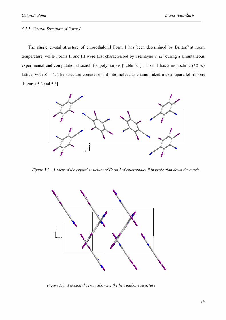
5.1.1 Crystal Structure of Form I
The single crystal structure of chlorothalonil Form I has been determined by Britton3 at room
temperature, while Forms II and III were first characterised by Tremayne et al2 during a simultaneous
experimental and computational search for polymorphs [Table 5.1]. Form I has a monoclinic (P21/a)
lattice, with Z = 4. The structure consists of infinite molecular chains linked into antiparallel ribbons
[Figures 5.2 and 5.3].
Figure 5.2. A view of the crystal structure of Form I of chlorothalonil in projection down the a axis.
Figure 5.3. Packing diagram showing the herringbone structure
Chlorothalonil Liana Vella-Żarb
74

5.1.2 Crystal Structure Prediction
In contrast with imidazole, chlorothalonil is a more challenging molecule with respect to crystal
structure prediction. This is due to its dominant Cl----N interactions being directional4. Although not
widely discussed, these short cyanohalide interactions are commonly found where X is Cl or Br, and
they arise due to halogen polarizability5. The computer modelling was based on a rigid chlorothalonil
molecule, using a molecular geometry obtained by ab initio optimisation of the SCF (Self-Consistent
Field, now better known as Hartree-Fock) wave function.
Initially, the computational search generated dense packings of the ab initio molecular structure of
chlorothalonil in 29 different crystal geometries. This resulted in a total of 1304 starting structures,
which were then used as starting points in the lattice energy minimization calculations, carried out using
the FIT potential6 [Figure 5.4].
The 27 structures found within 5 kJ mol-1 of the global minimum, i.e. the most energetically
favourable structures, were then reminimised using the ANI potential6. Some reordering of the relative
lattice energies was observed with the change in potential, and the number of distinct structures was
reduced to 22. This is due to the fact that some structures that were distinct minima with FIT converged
to the same minima for the ANI potential surface, lowering the symmetry in some of the cases. For both
potentials, however, the global minimum in the search corresponded with Form I.
Out of the 22 theoretical structures, 18 were found to have a Z’=1, and the remaining 4 structures
had Z’=2. The unit cell parameters of the 5 lowest energy structures are shown in [Table 5.1]. Most of
the theoretical structures were also found to have plate-like morphologies, with the largest dimension up
to ten times the thickness. When structures with such anisotropic behaviour are predicted, this may
indicate a possibility of preferred orientation being encountered during subsequent analysis by powder
diffraction. In such cases, this warning could suggest the adoption of capillary geometry during powder
diffraction data collection.
Chlorothalonil Liana Vella-Żarb
75

Table 5.1. The unit cell parameters of the five lowest energy structures for Chlorothalonil minimised using the ANI potential2.
SpaceGroup
Elatt (kJmol-1)
Cell Vol(Å3)
a(Å)
b(Å)
c(Å)
α (deg)
β (deg)
γ (deg)
exp
mina
FC45
AB15
AI44
AF18
AB3
P21/a -98.79 243.180 24.753 6.226 6.340 90.00 95.41 90.00
P21/a -99.40 243.246 24.840 6.272 6.288 90.00 96.65 90.00
Structures in search Reduced cell parameters
P21/c -99.40 243.243 24.839 6.288 6.272 90.00 96.65 90.00
P-1 -99.39 238.424 6.482 7.774 10.166 91.31 106.80 102.50
P21/c -99.31 243.379 12.750 12.309 6.228 90.00 95.12 90.00
P21 -99.02 243.922 12.486 6.302 6.235 90.00 95.31 90.00
P-1 -98.16 243.514 6.077 6.350 12.727 94.53 94.72 92.96
Chlorothalonil Liana Vella-Żarb
76
Figure 5.4 The distribution of some of the lower energy structures found in the search for minima in the lattice energy of chlorothalonil. The minimum corresponding to the known crystal structure of Form I
(Min from Expt) is denoted by the open red triangle7. [Permission for reproduction granted by the author of reference 7.]
!

5.2 Results
5.2.1 Low Temperature Data
The unit cell parameters of the predicted structure are similar to those of the published single crystal
structure obtained at room temperature. For this reason, the unit cell parameters from the published
single crystal structure were used as a starting point for a LeBail fit on the 293K data. The unit cell
parameters obtained from this initial fit were then used as a starting point for a LeBail fit on the 250K
data. Subsequent LeBail fits on the lower temperature data sets followed the same “stepwise”
methodology.
The powder diffraction pattern again illustrates a contraction in the unit cell with decreasing
temperature, as indicated by the clear shift in peak position (112) along 2θ [Figure 5.5] and across the
diffraction pattern from 5 to 45 along 2θ [Appendix A3.1].
Figure 5.5 Section of superimposed powder diffraction data at all temperatures showing peak (112) shifting towards the right with decreasing temperature.
2 θ / degrees
Inte
nsity
Chlorothalonil Liana Vella-Żarb
77

The percentage differences in a, b, c, β and volume with varying temperature were calculated and, as
expected, the volume increases as higher temperatures are reached, while a, b, c and β change
accordingly to accomodate this expansion [Table 5.2 and Figure 5.6].
Table 5.2 Unit cell parameters of the lowest energy predicted structure, those determined from experimental data, and published unit cell dimensions for chlorothalonil with changing temperature. The numbers in brackets denote the percentage change with respect to those values obtained from the 100K data.
Temperature (K) a (Å) b (Å) c (Å) β(o) Volume (Å3)
Single Crystal Values3 24.753(1) 6.226(1) 6.340(2) 95.41(3) 972.719
Predicted values2 (0K) 6.272(2) 6.288(1) 24.839(1) 96.65(1) 975.247
100(% change)
24.552 (1)(0.00)
6.183(2)(0.00)
6.351(3)(0.00)
96.18(2)(0.00)
958.589(0.00)
150(% change)
24.623(1)(+0.29)
6.175(2)(-0.13)
6.351(3)(-0.01)
95.89(2)(-0.29)
960.534(+0.20)
200(% change)
24.705(1)(+0.62)
6.225(1)(+0.67)
6.325(4)(-0.39)
95.85(3)(-0.34)
967.743(+0.95)
250(% change)
24.687(1)(+0.55)
6.231(1)(+0.77)
6.328(2)(-0.36)
95.62(2)(-0.58)
968.687(+1.05)
293(% change)
24.739(2)(+0.76)
6.233(3)(+0.80)
6.328(3)(-0.36)
95.34(1)(-0.87)
971.612(+1.36)
293 (D5000)(% change)
24.749(3)(+0.80)
6.228(2)(+0.72)
6.337(1)(-0.23)
95.40(2)(-0.81)
972.363(+1.44)
Chlorothalonil Liana Vella-Żarb
78

Over the range of temperatures, a and b increase overall while c generally shortens, perhaps to
accomodate the reduction of β. These changes in the lattice parameters result in an overall expansion of
the unit cell, as indicated by the increase in volume. As the material is anisotropic, overall cell volume
expansion is not necessarily a direct consequence of an increase in length in all directions. Again, as in
the case of imidazole, these change fluctuations could be due to the relative difference in intermolecular
interactions in each direction.
Chlorothalonil Liana Vella-Żarb
79
Figure 5.6 Graph showing the percentage change in unit cell dimensions with temperature.
!"#"$%
!"#""&%
"%
"#""&%
"#"$%
"#"$&%
$""% $&"% '""% '&"% '()%
*%
+%
,%
-./*%
01234.%
% c
hang
e
Temperature (K)

5.2.2 Automated Comparison
5.2.2.1 Rwp
The 22 minimised predicted structures were each compared, using Rwp, with the experimental data
collected at each temperature. The outcome of these comparisons was, as in the case of imidazole, non-
discriminatory, with none of the 22 structures identified as being significantly similar to any of the
experimental data sets. Rwp values ranging from 68.08% to 78.68% were obtained, with the lower
values resulting from comparison with the data collected at 200K [Table 5.3, Figure 5.7 and 5.8].
Identification of the correct predicted structure (fc45) would have been impossible based purely on these
Rwp values. A comparison of these predicted structure data sets with the experimental data is given in
Appendix A3.2.
Table 5.3. Structures with lowest Rwp identified at each temperature. The difference is that between the Rwp for the top ranked structure [Rwp(x)] and the correct prediction [Rwp(fc45)]. Red numbers denote incorrect structures ranked as the best.
Temperature (K) Top ranked
structure
Rwp (x) (%) Rwp (fc45) (%) Difference (%)[Rwp(x) - Rwp(fc45)]
100
150
200
250
293
D5000
az19 72.3 74.1 -1.8
bd13 68.9 69.2 -0.3
fc47 68.1 68.4 -0.3
fc48 72.5 73.0 -0.5
az19 73.9 76.1 -2.2
ab37 72.9 77.4 -4.5
Chlorothalonil Liana Vella-Żarb
80

Rwp (%)
ab3
ab11
ab15
ab25
ab27
ab36
ab37
af18
ai44
ak17
am12
am14
az19
bf4
fc4
fc45
fc47
fc48
bd13
dc35
dd42
de17
Stru
ctur
e
Chlorothalonil Liana Vella-Żarb
81
Figure 5.7 Rwp values for each structure at each temperature. The arrow indicates structure fc45.

Rwp (%)
ab3
ab11
ab15
ab25
ab27
ab36
ab37
af18
ai44
ak17
am12
am14
az19
bf4
fc4
fc45
fc47
fc48
bd13
dc35
dd42
de17
Stru
ctur
e
Chlorothalonil Liana Vella-Żarb
82
Figure 5.8 Rwp values for each structure against the D5000 data at room temperature. The arrow indicates structure fc45.

5.2.2.2 PolySNAP
Figure 5.9. Dendrogram showing similarity clusters for chlorothalonil predicted and D5005 experimental powder patterns
For PolySNAP analysis, the data collected on the different diffractometers were analysed separately
due to the difference in wavelength between the two setups. In the dendrogram comparing all 22
structures with the D5005 data [Figure 5.9], structure fc45, which corresponds to the published
structure, was grouped with the entire set of experimental data collected at all temperatures (cluster
shown in red in Figure 5.9). Also grouped in the same set, albeit at a higher tie-bar level, were
structures af18, ai44 and fc47. Although these powder patterns show similarities to the experimental
data, it is clear that the powder pattern from structure fc45, bears a more significant resemblance
[Figure 5.10 and Appendix A3.3]. As in the case of imidazole, the experimental data are all grouped
together, and within this cluster were paired subsets, with the data from lower temperatures ranked as
more similar to each other than the higher temperatures. Considering each temperature separately, and
Chlorothalonil Liana Vella-Żarb
83

looking at the structure with the highest correlation in each case, structure fc45 was the top-ranked
structure at all temperatures below 250K [Table 5.4].
Table 5.4. Structures with highest correlation coefficient [P(x)] at each temperature, and the difference to the value obtained for the correct structure [P(fc45)]. If P(fc45) = P(x), then the difference between P(fc45) and the next best structure is taken. Black numbers denote cases where the correct structure was identified, and the difference was positive. An incorrect match gave a negative difference, as shown by the values in red.
Temperature (K) Top ranked
structure
Correlation coefficient of top ranked structure
Correlation coefficient
Difference[P(fc45) - P(x)]
100
150
200
250
293
293 (D5000)
fc45 0.4639 0.4534 (fc4) 0.0105
fc45 0.5697 0.4292 (ai44) 0.1405
fc45 0.6167 0.3966 (ai44) 0.2201
ai44 0.4347 0.4046 (fc45) -0.0301
ai44 0.5583 0.2377 (fc45) -0.3206
af18 0.0675 -0.0564 (fc45) -0.1239
Although at higher temperatures an incorrect structure was ranked first, taking the values obtained
for the lower temperatures up to 200K the general trend observed with imidazole was retained. The
correlation plot [Figures 5.11 and 5.12 and Table 5.4] clearly illustrates that up to 200K, the degree of
similarity between the predicted structure fc45 and the experimental data increases with a rise in
temperature; the higher temperatures (up to 200K) also show better discriminating ability denoted by a
greater difference [P(fc45) - P(x)] between the correlation value obtained for the correct structure (fc45)
and the next best ranking structure. Visually, correlation plots at each temperature show a clear trend
which is retained as temperature varies. At higher temperatures an incorrect structure was identified as
being most similar. This mismatch could be attributed to the fact that predictions were carried out at
0K, and therefore lower temperature powder data would naturally bear higher correlation with the
simulated powder pattern than higher temperature data would.
Chlorothalonil Liana Vella-Żarb
84

Figure 5.10 Powder diffraction patterns for five selected predicted structures and the experimental structure at room temperature (D5005).
Chlorothalonil Liana Vella-Żarb
85
Intensity
2 θ
/ deg
rees
0
10000
20000
30000
40000
50000
60000
70000 1
0
15
20
25
30
35
40
45
50
55
60
fc45
af1
8
ai4
4
fc4
fc47
293K
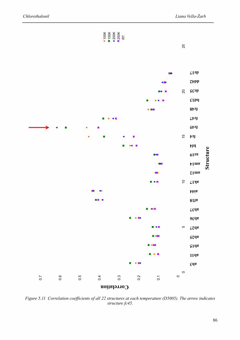
Correlation
ab3
ab11
ab15
ab25
ab27
ab36
ab37
af18
ai44
ak17
am12
am14
az19
bf4
fc4
fc45
fc47
fc48
bd13
dc35
dd42
de17
Stru
ctur
e
0
0.1
0.2
0.3
0.4
0.5
0.6
0.7
0
5
10
1
5
20
2
5
100K
150K
200K
250K
RT
Figure 5.11 Correlation coefficients of all 22 structures at each temperature (D5005). The arrow indicates structure fc45.
Chlorothalonil Liana Vella-Żarb
86
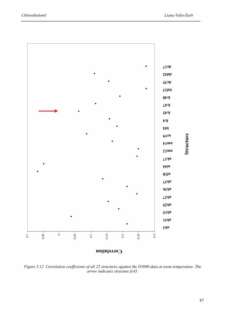
Correlation
ab3
ab11
ab15
ab25
ab27
ab36
ab37
af18
ai44
ak17
am12
am14
az19
bf4
fc4
fc45
fc47
fc48
bd13
dc35
dd42
de17
Stru
ctur
e
Figure 5.12 Correlation coefficients of all 22 structures against the D5000 data at room temperature. The arrow indicates structure fc45.
Chlorothalonil Liana Vella-Żarb
87
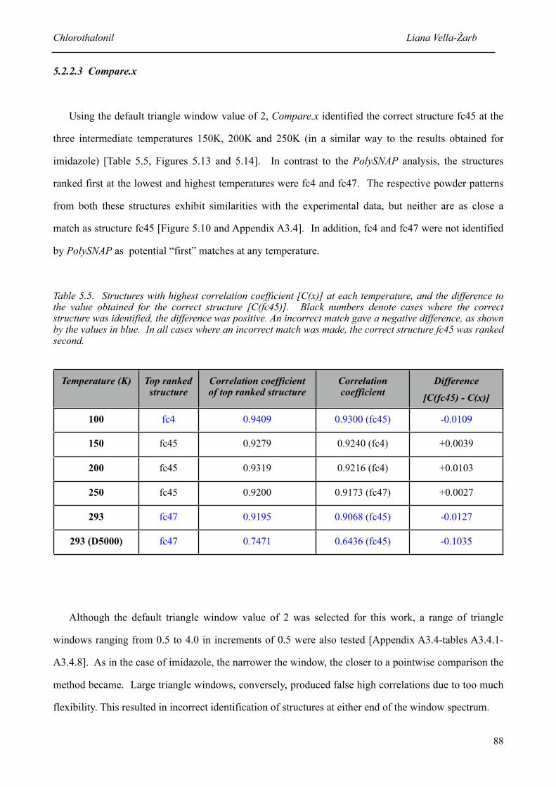
5.2.2.3 Compare.x
Using the default triangle window value of 2, Compare.x identified the correct structure fc45 at the
three intermediate temperatures 150K, 200K and 250K (in a similar way to the results obtained for
imidazole) [Table 5.5, Figures 5.13 and 5.14]. In contrast to the PolySNAP analysis, the structures
ranked first at the lowest and highest temperatures were fc4 and fc47. The respective powder patterns
from both these structures exhibit similarities with the experimental data, but neither are as close a
match as structure fc45 [Figure 5.10 and Appendix A3.4]. In addition, fc4 and fc47 were not identified
by PolySNAP as potential “first” matches at any temperature.
Table 5.5. Structures with highest correlation coefficient [C(x)] at each temperature, and the difference to the value obtained for the correct structure [C(fc45)]. Black numbers denote cases where the correct structure was identified, the difference was positive. An incorrect match gave a negative difference, as shown by the values in blue. In all cases where an incorrect match was made, the correct structure fc45 was ranked second.
Temperature (K) Top ranked structure
Correlation coefficient of top ranked structure
Correlation coefficient
Difference[C(fc45) - C(x)]
100
150
200
250
293
293 (D5000)
fc4 0.9409 0.9300 (fc45) -0.0109
fc45 0.9279 0.9240 (fc4) +0.0039
fc45 0.9319 0.9216 (fc4) +0.0103
fc45 0.9200 0.9173 (fc47) +0.0027
fc47 0.9195 0.9068 (fc45) -0.0127
fc47 0.7471 0.6436 (fc45) -0.1035
Although the default triangle window value of 2 was selected for this work, a range of triangle
windows ranging from 0.5 to 4.0 in increments of 0.5 were also tested [Appendix A3.4-tables A3.4.1-
A3.4.8]. As in the case of imidazole, the narrower the window, the closer to a pointwise comparison the
method became. Large triangle windows, conversely, produced false high correlations due to too much
flexibility. This resulted in incorrect identification of structures at either end of the window spectrum.
Chlorothalonil Liana Vella-Żarb
88

Correlation
ab3
ab11
ab15
ab25
ab27
ab36
ab37
af18ai44
ak17am12am14
az19
bf4
fc4
fc45
fc47
fc48
bd13
dc35
dd42
de17
Stru
ctur
e
Figure 5.13 Correlation coefficients of all 22 structures at each temperature. The arrow indicates structure fc45.
Chlorothalonil Liana Vella-Żarb
89

Correlation
ab3
ab11
ab15
ab25
ab27
ab36
ab37
af18
ai44
ak17
am12
am14
az19
bf4
fc4
fc45
fc47
fc48
bd13
dc35
dd42
de17
Stru
ctur
e
Figure 5.14. Correlation coefficients of all 22 structures against the D5000 data at room temperature. The arrow indicates structure fc45.
Chlorothalonil Liana Vella-Żarb
90

5.3 Discussion
Table 5.6. Comparison of the ability of the three methods in automated identification of the correct predicted structure. Values in red denote the difference (modulus of the difference for Rwp) between the correct structure and the structure ranked first. If the correct structure ranked first, then the values denote the difference between the correct structure and the next best one (shown in black).
Temperature (K) Rwp PolySNAP Compare.x
100 1.8 0.0105 0.0109
150 0.3 0.1405 0.0039
200 0.3 0.2201 0.0103
250 0.5 0.0301 0.0027
293 2.2 0.3206 0.0127
293 (D5000) 4.5 0.1239 0.1035
Rwp again failed to identify the correct structure and instead selected top-ranked structures with
powder diffraction data bearing little resemblance to that from the correct structure [Appendix A3.2].
With the more temperature-sensitive methods, only lower temperatures were found to correlate well
with the predicted structure [Table 5.6]. The reason behind this could possibly be zero point error, and
this would also explain why the room temperature data collected from the two different diffractometers
gave differing correlation values. As in the case of imidazole, Compare.x matched the correct
theoretical structure with the three intermediate temperatures.
In comparison with PolySNAP, Compare again gave higher overall correlation coefficients, and
although the discrimination between the highest ranking structure and the structure with the second
highest correlation coefficient increased with temperature there was less discrimination between the data
when compared with the values obtained from the PolySNAP analysis [Figure 5.15]. Notwithstanding
the fact that the incorrect structures were identified at higher temperatures, PolySNAP correlation values
increased with temperature. This further confirms the notion that PolySNAP comparative studies are
more sensitive to changes in temperature (and the resulting shifts in 2θ) as opposed to Compare.x.
Chlorothalonil Liana Vella-Żarb
91

Diff
eren
ce
Temperature (K)
Figure 5.15 Difference in correlation coefficients between fc45 and the structure with the next highest correlation. In cases where fc45 was not ranked first, the difference between fc45 and the structure with the
highest correlation is shown.
While Compare.x maintained a fairly consistent degree of discrimination over the range of
temperatures, PolySNAP’s discriminating ability showed a marked sensitivity to temperature up to
200K.
Despite the fact that predictions were carried out at low temperatures, both PolySNAP and
Compare.x analysis resulted in the highest correlation between the correct predicted structure and the
experimental data being found at 200K. As in the case of imidazole, this could imply that a zero point
error, resulting in a considerable shift in 2θ, may be distorting the results away from the better matches
at the expected temperatures. Again, predefining a reliably measurable zero point error before a
PolySNAP comparison is run would minimise this discrepancy. This can only be done with a
reasonably consistent zero point error.
Chlorothalonil Liana Vella-Żarb
92

5.4 References
1. Farm Chemical Handbook 2002: Global Guide to Crop Protection, Meister Publishing, Willoughby,
OH, 2002.
2. M. Tremayne, L. Grice, C. Pyatt, C. C. Seaton, B. M. Kariuki, H. H. Y. Tsui, S. L. Price and J. C.
Cherryman, J. Am. Chem. Soc., 2004, 126, 7071
3. D. Britton, Cryst. Struct. Commun., 1981, 10, 1501
4. J. P. Lommerse, A. J. Stone, R. Taylor and F. H. Allen, J. Am. Chem. Soc., 1996, 118, 3108
5. G. R. Desiraju and R. L. Harlow, J. Am. Chem. Soc., 1989, 111 (17), 6757
6. G. M. Day, S. L. Price and M. Leslie, Cryst. Growth Des., 2001, 1, 3
7. D. Britton, Acta Cryst. B, 2002, 58, 553
Chlorothalonil Liana Vella-Żarb
93

6. 5-AZAURACIL
Figure 6.1. 5-Azauracil (1,3,5-triazine-2,4(1H,3H)-dione)
H
H
H
O
ON
N
N
6.1 Background
5-Azauracil, a white crystalline colourless solid, is the aza analogue of the pyrimidine uracil,
one of the bases found in ribonucleic acid (RNA). Azapyrimidines (for example 5-azauracil and
its isomer 6-azauracil) differ from the nucleic acid bases in that they have a nitrogen instead of a
carbon atom at some position on the heterocyclic ring. When introduced at a strategic location on
the ring, this apparently minor change causes major electronic perturbation in the vicinity of the
substitution thus changing the structural, physico-chemical, and subsequently biological
properties of the base.
Purine and pyrimidine analogues (especially aza analogues of uracil1,2) are of particular
interest due to their potential uses as antineoplastic agents3,4 and enzyme inhibitors5. They also
exhibit bacteriostatic and fungicidal6,7 properties, and can be used in molecular biology protocols8
and as reagents for mutagenicity testing in microbial systems9.
5-Azauracil is of significant biological importance as it is a specific inhibitor of orotate
phosphoribosyl transferase, an enzyme involved in nucleic acid synthesis in vivo. Its biological
effects differ significantly from those of other closely-related azapyrimidines, such as 6-
azauracil10.
5-Azauracil Liana Vella-Żarb
94

6.1.1 Crystal Structure
Figure 6.2. 5-Azauracil molecules forming chains along the b axis.
The crystal structure of 5-azauracil was determined from X-ray diffraction data at room
temperature10. It has the orthorhombic spacegroup Pbca, with 8 molecules in the unit cell. Both
the heterocyclic nitrogen and its neighbouring carbonyl group can accept hydrogen bonds giving
the material a propensity to form sheets. The crystal structure [Figure 6.2] consists of crinkled
layers held together by strong NH----O and NH----N hydrogen bonds and several weaker
intermolecular interactions. These sheets are approximately perpendicular to the a axis and are
stacked so that there is very minimal overlap of the molecules between the layers [Figure 6.3].
Unit cell parameters for 5-azauracil are given in Table 6.2.
6.1.2 Crystal Structure Prediction
If a crystal structure is predictable to a useful extent11, then any structurally-related molecule
should, in theory, also be “predictable”. 5-Azauracil is an isomer of 6-azauracil, a molecule that
had already been investigated computationally12. This situation prompted a blind test to assess the
methodology employed in finding probable packings of rigid molecules with a choice of hydrogen
donors and acceptors.
5-Azauracil Liana Vella-Żarb
95

Figure 6.3. A view of 5-azauracil down the a axis. (Hydrogen bonds NH...N are shown by the dotted lines in violet.)
The prediction of the structure of 5-azauracil was carried out given that the computational
search for 6-azauracil resulted in numerous distinct structures12, including some with different
atoms involved in the hydrogen bonding, and lying within 1 kJmol-1 of the global minimum. The
search for 5-azauracil was therefore expected to result in a lattice energy plot with the known
structure among a group of thermodynamically plausible structures.
The first search carried out in 1999 yielded 42 structures10, and a more recent and extensive
search (carried out by Price et al in 2004)13 resulted in 49 theoretical structures, with the lower
energy structures corresponding to those obtained in the earlier search [Figure 6.4 and Table 6.1].
5-Azauracil Liana Vella-Żarb
96
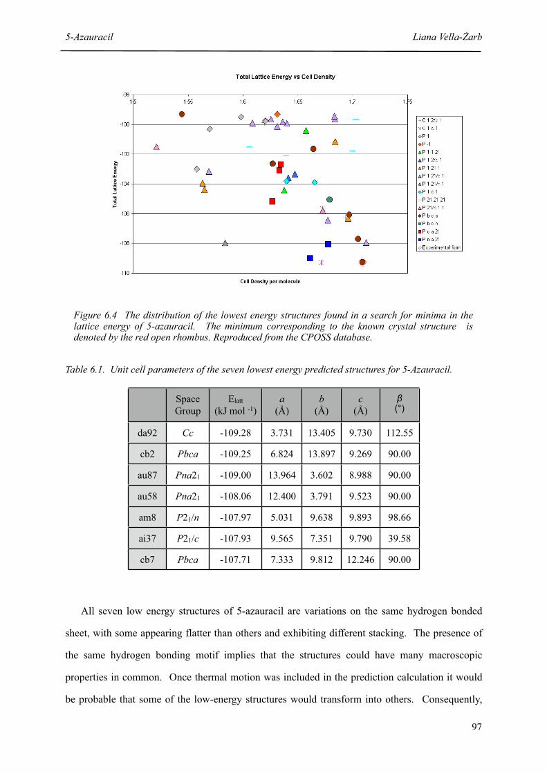
Figure 6.4 The distribution of the lowest energy structures found in a search for minima in the lattice energy of 5-azauracil. The minimum corresponding to the known crystal structure is denoted by the red open rhombus. Reproduced from the CPOSS database.
Table 6.1. Unit cell parameters of the seven lowest energy predicted structures for 5-Azauracil.
SpaceGroup
Elatt (kJ mol -1)
a(Å)
b(Å)
c(Å)
β (°)
da92
cb2
au87
au58
am8
ai37
cb7
Cc -109.28 3.731 13.405 9.730 112.55
Pbca -109.25 6.824 13.897 9.269 90.00
Pna21 -109.00 13.964 3.602 8.988 90.00
Pna21 -108.06 12.400 3.791 9.523 90.00
P21/n -107.97 5.031 9.638 9.893 98.66
P21/c -107.93 9.565 7.351 9.790 39.58
Pbca -107.71 7.333 9.812 12.246 90.00
All seven low energy structures of 5-azauracil are variations on the same hydrogen bonded
sheet, with some appearing flatter than others and exhibiting different stacking. The presence of
the same hydrogen bonding motif implies that the structures could have many macroscopic
properties in common. Once thermal motion was included in the prediction calculation it would
be probable that some of the low-energy structures would transform into others. Consequently,
5-Azauracil Liana Vella-Żarb
97

this predicts that it is unlikely that polymorphs of 5-azauracil having very different physical
properties would be readily found. Predicted structure da92, which has almost the same energy as
the experimentally known form, is polar. The crystal dipole correction term is likely to destabilise
this structure, leaving the known structure as the most stable. Cb2 is the correct predicted
structure, and it corresponds with the experimentally known form.
6.2 Results
6.2.1 Low Temperature Data
On visual comparison, the powder pattern collected at room temperature is similar to the
simulated patterns from both the published structure and the correct predicted structure cb2
[Figure 6.5 and Table 6.2]. Initially, a LeBail fit was carried out on the room temperature data
using the unit cell parameters from the published structure as a starting point. Subsequent LeBail
fits were carried out on the remainder of the data obtained using the same methodology. Although
the unit cell volume decreased with temperature, there was a marked difference between the
volume of the published structure which was collected at room temperature, and the volume of the
structure obtained experimentally at the same temperature. For this reason, all the data obtained
over the range of temperatures were indexed, and LeBail fits were subsequently carried out on the
indexed data. The volume of the unit cell obtained from the data at room temperature after
indexing was very close to the volume of the published structure. Consequently the indexed data
were used for the rest of this study.
5-Azauracil Liana Vella-Żarb
98

2 θ
/ deg
rees
Intensity
Figure 6.5 Simulated powder patterns for the published single crystal (SX) structure, the correct predicted structure cb2, predicted structure aq62, and the D5000 experimental data recorded at room
temperature (RT).
5-Azauracil Liana Vella-Żarb
99

Temperature (K) a (Å) b (Å) c (Å) Volume (Å3)
Published values (298K)10 6.514 (3) 13.522 (4) 9.582 (4) 843.96 (6)
Predicted values (0K) 6.824 13.897 9.269 879.01
10 6.385 (1)(0.00)
13.513 (3)(0.00)
9.547 (1)(0.00)
823.78 (1)(0.00)
100(% change)
6.398 (1)(+0.21)
13.523 (2)(+0.07)
9.560 (1)(+0.13)
827.12 (4)(+0.40)
150(% change)
6.425 (1)(+0.63)
13.487 (1)(-0.20)
9.549 (3)(+0.02)
827.48 (1)(+0.45)
200(% change)
6.433 (1)(+0.75)
13.491 (3)(-0.16)
9.575 (1)(+0.02)
828.76 (2)(+0.60)
250(% change)
6.490 (1)(+1.65)
13.526 (1)(+0.09)
9.579 (2)(+0.29)
840.57 (1)(+2.04)
293(% change)
6.514 (3)(+2.02)
13.513 (1)(-0.01)
9.646 (1)(+0.33)
843.09 (2)(+2.34)
293 (D5000) 6.513 (3)(+2.00)
13.512 (2)(-0.01)
9.575 (2)(+0.29)
842.65 (3)(+2.29)
The powder diffraction patterns indicate a clear contraction in the unit cell with decreasing
temperature, as shown by the clear shift in peak position (200) towards the right [Figure 6.6].
This change can be observed over the range of 5 to 45 degrees along 2θ for the full set of
experimental data in Appendix A4.1. The percentage differences in a, b, c and volume with
varying temperature were calculated and as expected, the volume decreased with lower
temperatures. Values for a also decreased uniformly while b and c fluctuated to accomodate this
contraction. Over the temperature range studied, the unit cell volume would be expected to
increase as a result of thermal expansion. Although b and c exhibited atypical fluctuations, these
changes in the lattice parameters still resulted in an overall expansion of the unit cell with
temperature, as indicated by the increase in volume [Figure 6.7].
Table 6.2 Unit cell parameters of the published crystal structure, correct predicted structure and those extracted from the experimental data over a range of temperatures. The numbers in brackets denote the percentage change with respect to those values obtained from the 10K data.
5-Azauracil Liana Vella-Żarb
100

Figure 6.6 Section of superimposed powder diffraction data at all temperatures showing peak (200) shifting towards the right with decreasing temperature. The predicted
structure (cb2) is indicated by the red dotted line.
2 θ / degrees
Intensity
Figure 6.7 Graph showing the percentage change in unit cell dimensions with temperature.
% c
hang
e
Temperature (K)
5-Azauracil Liana Vella-Żarb
101
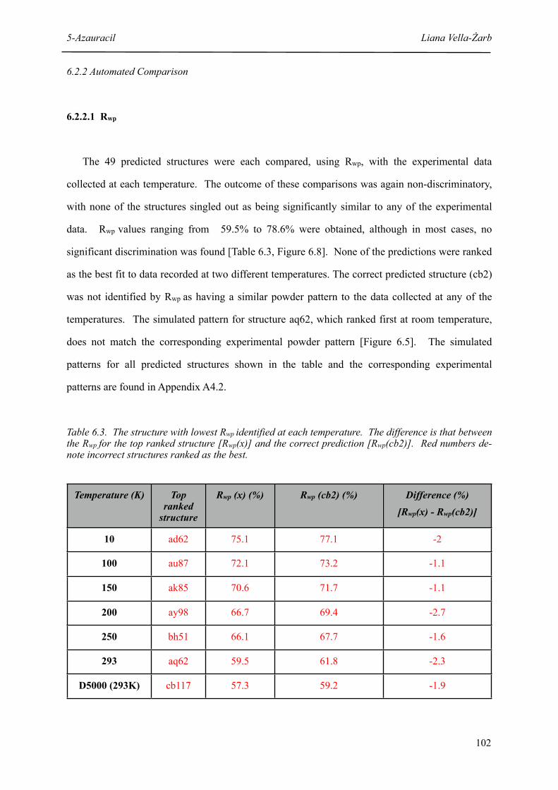
6.2.2 Automated Comparison
6.2.2.1 Rwp
The 49 predicted structures were each compared, using Rwp, with the experimental data
collected at each temperature. The outcome of these comparisons was again non-discriminatory,
with none of the structures singled out as being significantly similar to any of the experimental
data. Rwp values ranging from 59.5% to 78.6% were obtained, although in most cases, no
significant discrimination was found [Table 6.3, Figure 6.8]. None of the predictions were ranked
as the best fit to data recorded at two different temperatures. The correct predicted structure (cb2)
was not identified by Rwp as having a similar powder pattern to the data collected at any of the
temperatures. The simulated pattern for structure aq62, which ranked first at room temperature,
does not match the corresponding experimental powder pattern [Figure 6.5]. The simulated
patterns for all predicted structures shown in the table and the corresponding experimental
patterns are found in Appendix A4.2.
Table 6.3. The structure with lowest Rwp identified at each temperature. The difference is that between the Rwp for the top ranked structure [Rwp(x)] and the correct prediction [Rwp(cb2)]. Red numbers de-note incorrect structures ranked as the best.
Temperature (K) Top ranked
structure
Rwp (x) (%) Rwp (cb2) (%) Difference (%)[Rwp(x) - Rwp(cb2)]
10
100
150
200
250
293
D5000 (293K)
ad62 75.1 77.1 -2
au87 72.1 73.2 -1.1
ak85 70.6 71.7 -1.1
ay98 66.7 69.4 -2.7
bh51 66.1 67.7 -1.6
aq62 59.5 61.8 -2.3
cb117 57.3 59.2 -1.9
5-Azauracil Liana Vella-Żarb
102

Rwp (%)
Stru
ctur
e
ad5ad62ah6ai37ai46aj76ak53ak85al87
am50am8aq3
aq62aq71aq85ar42ar68au58au87av53ay36ay49ay93ay95ay98bh35bh51ca88
cb115cb117cb121
cb2cb7
cc72cd107 cd14cd45ce48ce76da59da92dd71de90fa22fa27fa41fa53fc25fc54
Figure 6.8 Rwp values for each predicted structure at each temperature (D5005). The arrow indicates structure cb2.
5-Azauracil Liana Vella-Żarb
103

6.2.2.2 PolySNAP
Figure 6.9. Dendrogram showing similarity clusters for 5-azauracil predicted and experimental powder patterns
For PolySNAP analysis, the data collected on the different diffractometers were analysed
separately due to the difference in wavelength between the two machines. In the dendrogram
above, all 49 predicted structures are compared with the D5005 data [Figure 6.9]. Structures cb2
and aq85 were grouped as most similar to the experimental data collected at all temperatures, and
slightly lower on the similarity scale is structure aq62. Once again, although all experimental data
sets were grouped together, there is clear clustering into paired subsets with the lower temperature
data pair (10K and 100K) being ranked as more similar to each other than the next highest. On
analysis of each temperature separately and consideration of the structure with the highest
correlation in each case, structure aq85 was ranked as the most similar to the experimental data at
10K and 100K, while structure cb2 was identified as a match at temperatures of 150K and above
[Table 6.4].
5-Azauracil Liana Vella-Żarb
104
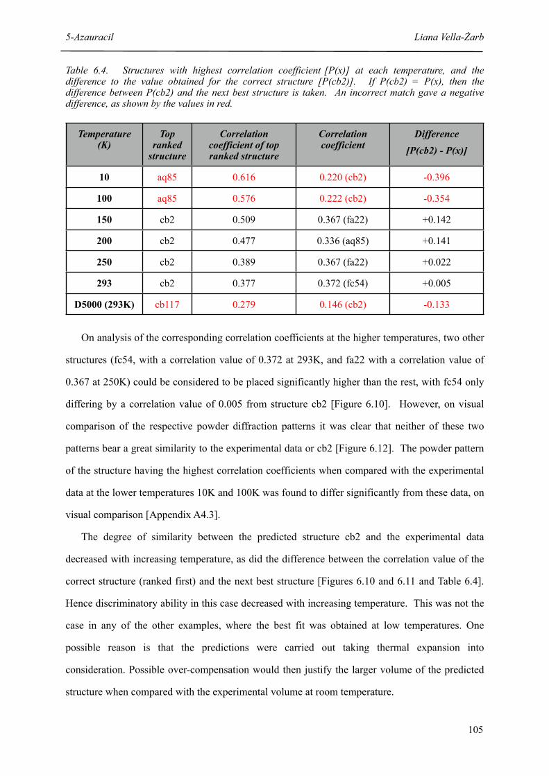
Table 6.4. Structures with highest correlation coefficient [P(x)] at each temperature, and the difference to the value obtained for the correct structure [P(cb2)]. If P(cb2) = P(x), then the difference between P(cb2) and the next best structure is taken. An incorrect match gave a negative difference, as shown by the values in red.
Temperature (K)
Top ranked
structure
Correlation coefficient of top ranked structure
Correlation coefficient
Difference[P(cb2) - P(x)]
10
100
150
200
250
293
D5000 (293K)
aq85 0.616 0.220 (cb2) -0.396
aq85 0.576 0.222 (cb2) -0.354
cb2 0.509 0.367 (fa22) +0.142
cb2 0.477 0.336 (aq85) +0.141
cb2 0.389 0.367 (fa22) +0.022
cb2 0.377 0.372 (fc54) +0.005
cb117 0.279 0.146 (cb2) -0.133
On analysis of the corresponding correlation coefficients at the higher temperatures, two other
structures (fc54, with a correlation value of 0.372 at 293K, and fa22 with a correlation value of
0.367 at 250K) could be considered to be placed significantly higher than the rest, with fc54 only
differing by a correlation value of 0.005 from structure cb2 [Figure 6.10]. However, on visual
comparison of the respective powder diffraction patterns it was clear that neither of these two
patterns bear a great similarity to the experimental data or cb2 [Figure 6.12]. The powder pattern
of the structure having the highest correlation coefficients when compared with the experimental
data at the lower temperatures 10K and 100K was found to differ significantly from these data, on
visual comparison [Appendix A4.3].
The degree of similarity between the predicted structure cb2 and the experimental data
decreased with increasing temperature, as did the difference between the correlation value of the
correct structure (ranked first) and the next best structure [Figures 6.10 and 6.11 and Table 6.4].
Hence discriminatory ability in this case decreased with increasing temperature. This was not the
case in any of the other examples, where the best fit was obtained at low temperatures. One
possible reason is that the predictions were carried out taking thermal expansion into
consideration. Possible over-compensation would then justify the larger volume of the predicted
structure when compared with the experimental volume at room temperature.
5-Azauracil Liana Vella-Żarb
105

Figure 6.10 Correlation coefficients of all 49 structures at each temperature (D5005). The arrow indicates structure cb2.
5-Azauracil Liana Vella-Żarb
106
Correlation
Stru
ctur
e
ad5ad62ah6ai37ai46aj76ak53ak85al87
am50am8aq3
aq62aq71aq85ar42ar68au58au87av53ay36ay49ay93ay95ay98bh35bh51ca88
cb115cb117cb121
cb2cb7
cc72cd107 cd14cd45ce48ce76da59da92dd71de90fa22fa27fa41fa53fc25fc54
-0.1
0
0.1
0.2
0.3
0.4
0.5
0.6
0.7
10
K
10
0K
15
0K
20
0K
25
0K
RT

ad5ad62ah6ai37ai46aj76ak53ak85al87
am50am8aq3
aq62aq71aq85ar42ar68au58au87av53ay36ay49ay93ay95ay98bh35bh51ca88
cb115cb117cb121
cb2cb7
cc72cd107 cd14cd45ce48ce76da59da92dd71de90fa22fa27fa41fa53fc25fc54
Correlation
Stru
ctur
e
Figure 6.11 Correlation coefficients of all 49 structures against the D5000 data. The arrow indicates structure cb2.
5-Azauracil Liana Vella-Żarb
107
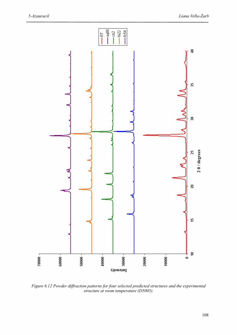
Intensity
2 θ
/ deg
rees
Figure 6.12 Powder diffraction patterns for four selected predicted structures and the experimental structure at room temperature (D5005).
5-Azauracil Liana Vella-Żarb
108
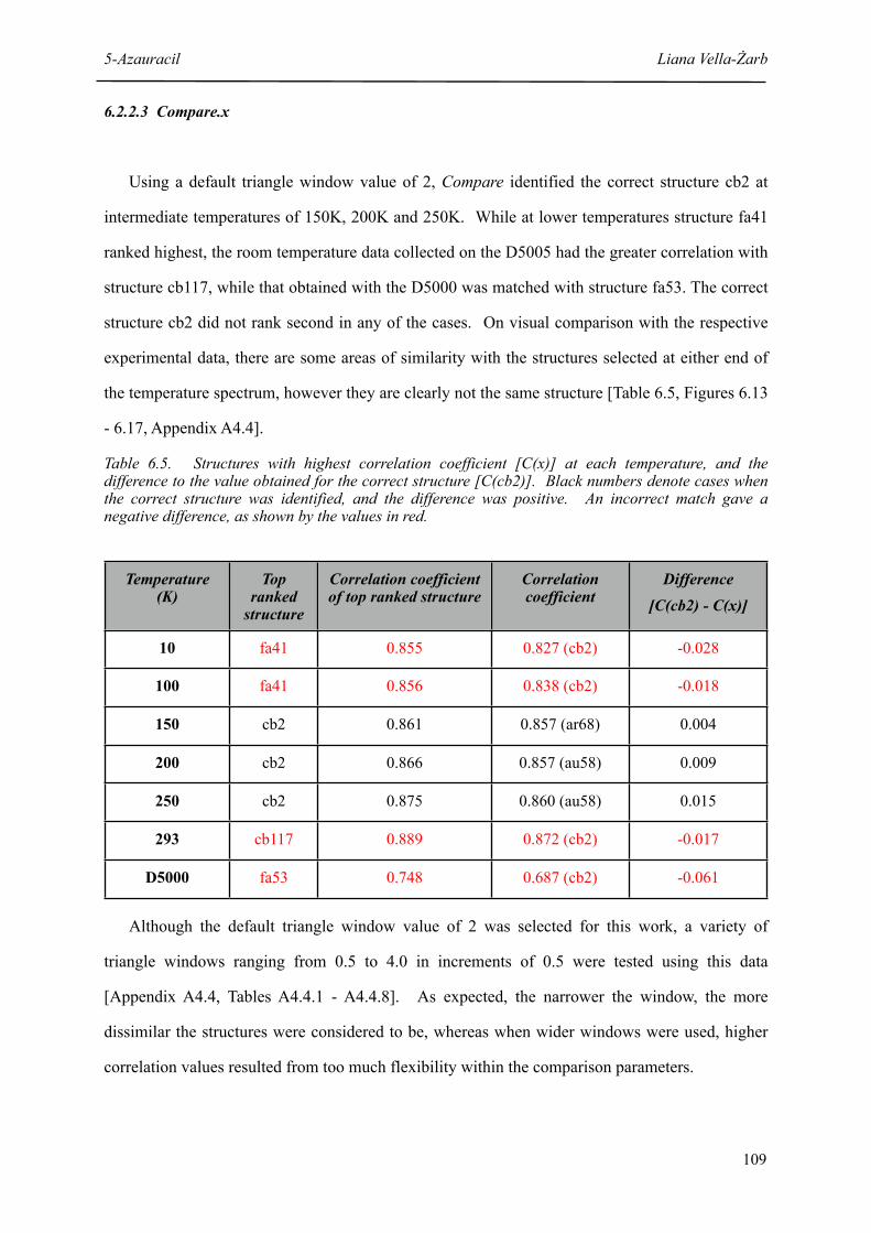
6.2.2.3 Compare.x
Using a default triangle window value of 2, Compare identified the correct structure cb2 at
intermediate temperatures of 150K, 200K and 250K. While at lower temperatures structure fa41
ranked highest, the room temperature data collected on the D5005 had the greater correlation with
structure cb117, while that obtained with the D5000 was matched with structure fa53. The correct
structure cb2 did not rank second in any of the cases. On visual comparison with the respective
experimental data, there are some areas of similarity with the structures selected at either end of
the temperature spectrum, however they are clearly not the same structure [Table 6.5, Figures 6.13
- 6.17, Appendix A4.4].
Table 6.5. Structures with highest correlation coefficient [C(x)] at each temperature, and the difference to the value obtained for the correct structure [C(cb2)]. Black numbers denote cases when the correct structure was identified, and the difference was positive. An incorrect match gave a negative difference, as shown by the values in red.
Temperature (K)
Top ranked
structure
Correlation coefficient of top ranked structure
Correlation coefficient
Difference[C(cb2) - C(x)]
10
100
150
200
250
293
D5000
fa41 0.855 0.827 (cb2) -0.028
fa41 0.856 0.838 (cb2) -0.018
cb2 0.861 0.857 (ar68) 0.004
cb2 0.866 0.857 (au58) 0.009
cb2 0.875 0.860 (au58) 0.015
cb117 0.889 0.872 (cb2) -0.017
fa53 0.748 0.687 (cb2) -0.061
Although the default triangle window value of 2 was selected for this work, a variety of
triangle windows ranging from 0.5 to 4.0 in increments of 0.5 were tested using this data
[Appendix A4.4, Tables A4.4.1 - A4.4.8]. As expected, the narrower the window, the more
dissimilar the structures were considered to be, whereas when wider windows were used, higher
correlation values resulted from too much flexibility within the comparison parameters.
5-Azauracil Liana Vella-Żarb
109

Correlation
Stru
ctur
e
ad5ad62ah6ai37ai46aj76ak53ak85al87
am50am8aq3
aq62aq71aq85ar42ar68au58au87av53ay36ay49ay93ay95ay98bh35bh51ca88
cb115cb117cb121
cb2cb7
cc72cd107 cd14cd45ce48ce76da59da92dd71de90fa22fa27fa41fa53fc25fc54
Figure 6.13 Correlation coefficients of all 49 structures at each temperature. The arrow indicates structure cb2.
5-Azauracil Liana Vella-Żarb
110

Correlation
Stru
ctur
e
ad5ad62ah6ai37ai46aj76ak53ak85al87
am50am8aq3
aq62aq71aq85ar42ar68au58au87av53ay36ay49ay93ay95ay98bh35bh51ca88
cb115cb117cb121
cb2cb7
cc72cd107 cd14cd45ce48ce76da59da92dd71de90fa22fa27fa41fa53fc25fc54
Figure 6.14 Correlation coefficients of all 49 structures against the D5000 data. The arrow indicates structure cb2.
5-Azauracil Liana Vella-Żarb
111

Intensity
2 θ
/ deg
rees
Figure 6.15 Powder diffraction patterns for fa41 and the experimental structure at 10K and 100K.
5-Azauracil Liana Vella-Żarb
112

Intensity
2 θ
/ deg
rees
Figure 6.16 Powder diffraction patterns for cb117 and the experimental structure at room temperature.
5-Azauracil Liana Vella-Żarb
113
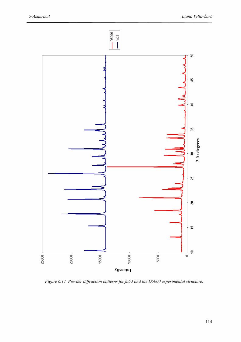
Intensity
2 θ
/ deg
rees
Figure 6.17 Powder diffraction patterns for fa53 and the D5000 experimental structure.
5-Azauracil Liana Vella-Żarb
114

6.3 Discussion
Table 6.6. Comparison of the ability of the three methods in automated identification of the correct predicted structure. Values in red denote the difference (modulus of the difference for Rwp) between the correct structure and the structure ranked first. If the correct structure ranked first, the values denote the difference between the correct structure and the next best one (shown in black).
Temperature (K) Rwp PolySNAP Compare
10 2 0.396 0.028
100 1.1 0.354 0.018
150 1.1 0.142 0.004
200 2.7 0.141 0.009
250 1.6 0.022 0.015
293 2.3 0.005 0.017
D5000 (293K) 1.9 0.133 0.061
The Rwp method once again yielded negative results, further proving its unreliability in
selecting correct predictions in relation to experimental powder data. Although Compare.x did
not identify cb2 as the correct structure at room temperature, the difference in correlation value
between cb2 and the next-ranking structure up to that temperature increased overall. Past 250K, a
different structure was selected, possibly implying a shift in 2θ that was large enough to enable
different peaks to fall within the confines of the triangle window.
In the cases where PolySNAP identified the correct structure, both correlation values and
discriminatory ability decreased markedly with temperature, the highest correlation between
experimental data and cb2 being observed at 150K. This corresponds with the temperature at
which there was the greatest discrimination between the correct structure (ranked first) and the
structure with the next best correlation.
5-Azauracil Liana Vella-Żarb
115

Diff
eren
ce
Temperature (K)
Figure 6.18 Difference in correlation coefficients between cb2 and the structure with the next highest correlation. In cases where cb2 was not ranked first, the difference between cb2 and the
structure with the highest correlation was plotted.
In comparison with PolySNAP, Compare.x once again gave higher overall correlation
coefficients and a greater discrimination with increasing temperature. Although the PolySNAP
comparison gave positive results at intermediate and higher temperatures suggesting an overall
sensitivity to the peak shift arising from expansion of the unit cell, the discrimination between the
correct structure and the structure with the second highest correlation coefficient did not show any
particular sensitivity to temperature [ Figure 6.18].
5-Azauracil Liana Vella-Żarb
116

6.4 References
1. J. Skoda, in D. Shugar (Ed.), Biochemical Aspects of Antimetabolites and Drug Hydroxylation,
Academic Press, New York, 1969 16, 29
2. J. K. Lindquist, in A. Katriztky, C. W. Rees (Eds.), Comprehensive Heterocyclic Chemistry,
Permagon Press, Oxford, 1984, 159
3. J. Beranek and E. M. Acton, Collect. Czech Chem. Commun., 1984, 49, 2551
4. L. H. Li, G. C. Neil, T. E. Morley and E. J. Olin, Cancer Chemotherapy Rep., 1974, Part 1 56,
345
5. J. Skoda, Prog. Nucl. Acid. Res., 1963, 2, 197
6. A. M. Gero, W. J. O’Sullivan and D. Brown, Biochem. Med., 1985, 34, 60
7. W. H. Prussoff and A. D. Welch, J. Biol. Chem., 1956, 218, 929
8. C. H. Schalbe and W. Saenger, J. Mol. Biol., 1973, 75, 129
9. A. El-Tarrass, R. Braun, E. Stenz and G. Schuster, Zentralblatt fur Mikrobiologie, 1989, 144,
197
10. B. S. Potter, R. A. Palmer, R. Withnall, B. Z. Chowdry and S. L. Price, J. Mol. Struct., 1999,
349, 485
11. A. Gavezzotti, Acc. Chem. Res., 1994, 27, 309
12. S. L. Price and K. S. Wibley, J. Phys. Chem. A, 1997, 101, 2198
13. A. E. Gray, G. M. Day, M Leslie and S L Price, Molecular Physics, 2004, 102 (9), 1067
5-Azauracil Liana Vella-Żarb
117

7. DNA BASES
Adenine and guanine are two of the nitrogen bases found in nucleic acids, along with the
pyrimidines cytosine (found in both DNA and RNA), uracil (found only in RNA) and thymine
(normally found in DNA, although sometimes tRNA will contain some thymine as well a uracil). The
hydrogen bonding interactions between purines and pyrimidines are among the core factors determining
the structure (and consequently also the function) of DNA. These hydrogen bonds formed by the base
pairs of adenine and thymine, and guanine and cytosine, constitute the “rungs” that are responsible for
the double helical nature of DNA. In this chapter, the structure solution and structure prediction
calculations of the two DNA purines will be discussed.
7.1 Adenine
Figure 7.1.1 Adenine (6-aminopurine)
N
H
NN
NNH
H
H
H
DNA Bases - Adenine Liana Vella-Żarb
118

7.1.1 Background
Besides DNA and RNA, adenine is also an important constituent of adenosine triphosphate (ATP).
It is essential due to its ability to phosphorylize, or add a phosphate group to other molecules. The
transfer of a phosphate group allows energy to be released, and it is this energy that is used by cells in
living organisms.
Although it is quite a high-profile molecule, the structure of adenine had not been previously
determined, and no evidence of polymorphism has been reported. However, structures with adenine
existing as a complex with riboflavin1, phthalic acid2, hydrogen peroxide3, and N-methyl-2-pyrrolidone4
can be found on the CSD. Other published structures include adenine in trihydrate form5 and in
adeninium tetrafluoroborate dihydrate6.
7.1.1.1 Experimental Polymorph Search7
An extensive polymorph search was carried out using 42 solvents7, and crystallisations were mainly
carried out by slow evaporation. The majority of solvents gave either no solid for analysis, or small
particles of solid that were unsuitable for characterisation purposes. Crystallisation from 2,2,2-
trifluoroethanol, acetic acid, dimethylamine in water and 2-methoxyethylamine yielded adenine as a
polycrystalline solid with a powder diffraction pattern that matched the stock sample. Adeninium
chloride hemihydrate and adeninium dichloride structures were also found in the search [Appendix A5.1
Table A5.1.1].
7.1.1.2 Computational Polymorph Searches7
In the computational polymorph search based on the ab initio molecular structure, 2900 structures
were generated, with 11 unique structures lying within 7 kJ mol-1 of the global lattice energy minimum.
A further search using the planar molecular structure resulted in 14 unique structures in the same energy
range7 [Table 7.1.1 and Figure 7.1.2], and 8 of which had Z’=2. The ab initio search found the structure
DNA Bases - Adenine Liana Vella-Żarb
119

am62 at the global lattice energy minimum, ~2 kJ mol-1 more stable than the next structure and with
about the same estimated energy difference at room temperature. Three hypothetical structures were
found within 4.5 kJ mol-1 of the global lattice energy minimum (this difference decreases to 2.5 kJ mol-1
at room temperature).
-144
-143
-142
-141
-140
-139
-138
-137
-136
-135
-1341.52 1.54 1.56 1.58 1.6 1.62 1.64
Cell Density per molecule
Tot
al L
attic
e E
nerg
y TOTAL LATTICEENERGY(kJ/mol) : opt
TOTAL LATTICEENERGY(kJ/mol) : planar
Experimental form
Ab initio
Figure 7.1.2 The results of both computational searches (ab initio and planar) showing the predicted structure corresponding to the experimental form denoted by the red open diamond. [Figure reproduced with
permission from the CPOSS database]
The computational search based on the planar molecular structure gave five unique hypothetical
structures with a range of densities, and lying within 1.2 kJ mol-1 of the global lattice energy minimum.
In both computational searches, all but one of the low energy structures consisted of hydrogen bonded
sheets. Three main types of sheet structure were identified, exhibiting only minor rearrangement of the
molecules in the sheets, attributed to the use of various combinations of donors and acceptors [Figure
7.1.3]. There were also slight changes in the orientation of the sheets relative to each other.
DNA Bases - Adenine Liana Vella-Żarb
120

Table 7.1.1. The low energy crystal structures found within 7 kJ mol-1 of the global lattice energy minimum for adenine, using the ab initio and planar molecular structures. All the structures consist of molecules that use N1, N2, and N3 as hydrogen bond acceptors, and all contain hydrogen bonded sheets, except for de56 which contains a three-dimensional hydrogen bonding network.
STRUCTURE SPACE GROUP
LATTICE ENERGY(kJ/mol)
FREE ENERGY(kJ/mol)
DENSITY(g/cm3)
REDUCED CELL
a(Å) b(Å) c(Å) α(°) β(°) γ(°)
Ab initio molecular structures
am62 P 21 /c -143.06 -152.26 1.6266 6.637 12.181 9.530 90.00 45.74 90.00
fc84 P 21 /c -141.43 -150.42 1.6019 4.696 8.167 14.846 90.00 79.73 90.00
cb24 P b c a -138.54 -149.74 1.5916 14.371 12.186 6.440 90.00 90.00 90.00
fc4 P 21 /c -138.41 -148.39 1.5498 4.718 8.164 21.824 90.00 43.55 90.00
ab102 P -1 -138.03 -147.06 1.6247 8.514 5.315 7.970 106.25 70.32 125.06
dc46 C 2/c -137.91 -146.97 1.5958 10.028 8.352 13.750 90.00 77.63 90.00
ab16 P -1 -137.43 -147.02 1.5636 8.541 4.596 8.136 98.65 114.38 89.73
dd101 C 2/c -136.97 -145.48 1.5459 6.884 12.223 23.829 90.00 35.39 90.00
am21 P 21 /c -136.68 -147.11 1.54 5.234 14.969 7.480 90.00 96.04 90.00
cd110 Pna21 -136.49 -148.03 1.5472 6.398 14.913 12.161 90.00 90.00 90.00
cb89 P -1 -136.38 -147.14 1.5877 7.027 13.230 12.161 90.00 90.00 90.25
Planar molecular structures
fc33 P 21 /c -142.87 -151.5 1.5973 4.851 8.092 14.600 90.00 101.36 90.00
am9 P 21 /c -142.46 -151.95 1.6048 6.458 12.170 7.121 90.00 88.14 90.00
ak71 P 21 /c -141.9 -150.93 1.562 6.650 7.862 12.390 90.00 62.49 90.00
cc71 P 21 /c -141.82 -152.81 1.5855 8.330 7.496 21.831 90.00 90.00 56.16
fc1 P 21 /c -141.69 -150.91 1.5519 4.879 7.871 21.999 90.00 43.21 90.00
aj80 P -1 -140.85 -150.03 1.5604 8.089 4.725 22.654 47.76 74.76 94.92
ce73 Pca21 -140.12 -150.42 1.5575 21.958 8.007 6.555 90.00 90.00 90.00
am43 P 21 /c -139.92 -150.47 1.5473 5.301 14.952 8.576 90.00 58.58 90.00
cb108 P 21 /c -139.84 -151.13 1.5407 12.221 14.943 6.736 90.00 71.28 90.00
ab72 P -1 -139.08 -148.09 1.617 8.492 4.926 8.426 103.83 73.81 124.48
bf37 P -1 -138.53 -148.59 1.5871 8.356 21.789 5.429 125.88 55.08 89.87
ai116 P 21 /c -138.49 -147.8 1.5827 8.832 8.112 8.382 90.00 70.79 90.00
ca73 P -1 -138.09 -147.51 1.5516 9.810 4.770 7.994 100.13 116.62 60.05
de56 C 2/c -136.98 -147.91 1.572 19.452 3.779 23.120 90.00 137.78 90.00
DNA Bases - Adenine Liana Vella-Żarb
121

I II III
Figure 7.1.3 The three different hydrogen bonded sheet structures present in the low energy structures in both computational polymorph searches on adenine
The majority of the elastic constants of the low energy structures were relatively low (<1 GPa),
possibly indicating a tendency for the hydrogen bonded sheets to slip over each other7. This would
decrease the mechanical stability, suggesting that the energetically favourable crystal packings of
adenine give relatively soft crystals, and could hence indicate problematic crystal growth.
7.1.2 Results
As an unknown crystal structure, attempts were made to index the experimental data and proceed
with a traditional structure solution. However, the data could not be indexed reliably, i.e. a suitable cell
could not be identified amongst the others in the indexing results. Therefore, the structure prediction
results were examined to establish whether these could be used to aid determination of this elusive
crystal structure.
7.1.2.1 PolySNAP
PolySNAP was used to identify any similarities between the experimental powder data and that
simulated for all the predicted structures. As low temperature data had not yet been recorded at this
early stage of the adenine study, the room temperature transmission data (D5000) was used for
comparison. The computational crystal structure cc71 (Z’ = 2) from the planar molecular structure
DNA Bases - Adenine Liana Vella-Żarb
122
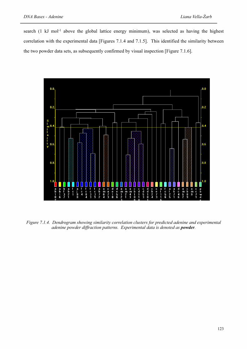
search (1 kJ mol-1 above the global lattice energy minimum), was selected as having the highest
correlation with the experimental data [Figures 7.1.4 and 7.1.5]. This identified the similarity between
the two powder data sets, as subsequently confirmed by visual inspection [Figure 7.1.6].
Figure 7.1.4. Dendrogram showing similarity correlation clusters for predicted adenine and experimental adenine powder diffraction patterns. Experimental data is denoted as powder.
DNA Bases - Adenine Liana Vella-Żarb
123
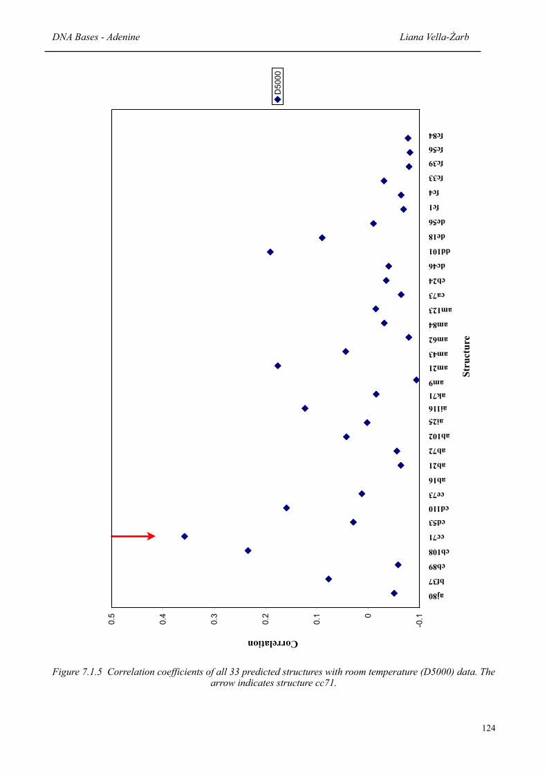
Correlation
Stru
ctur
e
-0.10
0.1
0.2
0.3
0.4
0.5
D5000
aj80
bf37
cb89
cb108
cc71
cd53
cd110
ce73
ab16
ab21
ab72
ab102
ai25ai116ak71am9
am21
am43
am62
am84
am123
ca73
cb24
dc46
dd101
de18
de56
fc1
fc4
fc33
fc39
fc56
fc84
Figure 7.1.5 Correlation coefficients of all 33 predicted structures with room temperature (D5000) data. The arrow indicates structure cc71.
DNA Bases - Adenine Liana Vella-Żarb
124

Intensity
2 θ
/ deg
rees
Figure 7.1.6 Powder diffraction patterns for two selected predicted structures and the experimental data (D5000) at room temperature.
DNA Bases - Adenine Liana Vella-Żarb
125

In order to complete the study of this structure and complete investigation of the effectiveness of
automated structure prediction comparison, the PolySNAP analysis was repeated using low temperature
data when this became available. Structure cc71 was identified as having the highest correlation to the
experimental data at each temperature [Table 7.1.2, Figure 7.1.8].
As observed in our other studies, the predicted structure (cc71) was found to have higher
correlation coefficients with experimental data collected at low temperatures than with data collected at
higher temperatures. The discrimination between structures ranked best and second did not vary widely
at the lower temperatures, though a slightly greater discrimination was observed with the 150K data. At
higher temperatures however, there was a reduction in discriminating ability, with the best two
structures exhibiting only marginal differences in correlation coefficients. Figure 7.1.7 shows the
simulated patterns of the best two structures and the experimental data at all temperatures.
Table 7.1.2. Correlation coefficient of the correct structure [P(cc71)] at each temperature, and the difference to the value obtained for the structure ranked second [P(x)]. In all cases, the correct structure (cc71) was identified.
Temperature (K) Top ranked
structure
Correlation coefficient of top ranked structure
Correlation coefficient
Difference[P(cc71) - P(x)]
10
50
100
150
200
250
293
293 (D5000)
cc71 0.5072 0.3622 (bf37) 0.1450
cc71 0.5356 0.4149 (bf37) 0.1207
cc71 0.5211 0.3817 (bf37) 0.1394
cc71 0.4875 0.3185 (bf37) 0.1690
cc71 0.3973 0.2448 (bf37) 0.1525
cc71 0.2997 0.2013 (fc84) 0.0984
cc71 0.2292 0.2240 (dd101) 0.0052
cc71 0.3581 0.2345 (cb108) 0.1236
DNA Bases - Adenine Liana Vella-Żarb
126

Intensity
2 θ
/ deg
rees
!"
#!!!!"
$!!!!"
%!!!!"
&!!!!"
'!!!!"
(!!!!"
)!!!!"
*!!!!"
+!!!!" #!"
#'"
$!"
$'"
%!"
%'"
&!"
,,)#"
#!-"
'!-"
#!!-"
#'!-"
$!!-"
$'!-"
./"
00#!#"
Figure 7.1.7 Powder diffraction patterns for two selected predicted structures and the experimental data (D5005) at all temperatures.
DNA Bases - Adenine Liana Vella-Żarb
127

Correlation
Stru
ctur
e
aj80
bf37
cb89
cb108
cc71
cd53
cd110
ce73
ab16
ab21
ab72
ab102
ai25ai116ak71am9
am21
am43
am62
am84
am123
ca73
cb24
dc46
dd101
de18
de56
fc1
fc4
fc33
fc39
fc56
fc84
-0.10
0.1
0.2
0.3
0.4
0.5
0.6
10K
50K
100K
150K
200K
250K
RT
Figure 7.1.8 Correlation coefficients of all 33 predicted structures at each temperature. The arrow indicates structure cc71.
DNA Bases - Adenine Liana Vella-Żarb
128

7.1.2.2 Compare.x
Using the default triangle window value of 2, Compare.x also identified the correct structure, cc71,
as having the highest correlation with the experimental data at all temperatures but 293K. The room
temperature data showed highest correlation with structure dd101, while cc71 was ranked second with a
difference of 0.02411 with the D5005 data, but even lower down the list when compared to the D5000
data [Table 7.1.3 and Figures 7.1.9 and 7.1.10].
Table 7.1.3. Structures with highest correlation coefficient [C(x)] at each temperature, and the difference to the value obtained for the correct structure [C(cc71)]. Black numbers denote cases where the correct structure was identified, and the difference was positive. An incorrect match gave a negative difference, as shown by the values in red and blue. Blue denotes cc71 being ranked second, while values in red correspond to cc71 being ranked third or lower.
Temperature (K) Top ranked structure
Correlation coefficient of top ranked structure
Correlation coefficient
Difference[C(cc71) - C(x)]
10
50
100
150
200
250
293
293 (D5000)
cc71 0.87413 0.81431 (ab21) 0.05982
cc71 0.87812 0.81961 (ab21) 0.05851
cc71 0.87276 0.81489 (ab21) 0.05787
cc71 0.86874 0.81522 (dd101) 0.05352
cc71 0.85485 0.81826 (dd101) 0.03659
cc71 0.83472 0.82841 (dd101) 0.00631
dd101 0.83534 0.81123 (cc71) -0.02411
dd101 0.72463 0.70376 (cc71) -0.02087
As the temperature increases, the unit cell expands and this translates as a shift in peak position along 2θ.
As the cc71 structure is predicted at 0K and Compare.x uses a triangular window approach to define the
correlation range, comparison with data recorded at 293K results in some of the peaks in the simulated cc71
powder pattern to fall outside the defined range. The powder diffraction pattern of structure dd101 has more
peaks than cc71 [Figure 7.1.6] and was identified as having the best correlation with the experimental data
purely on the basis of more peaks falling within the pre-defined triangle window. This “apparent” similarity
can be discounted upon visual comparison of the respective powder diffraction patterns.
DNA Bases - Adenine Liana Vella-Żarb
129

Correlation
Stru
ctur
e
0.4
0.5
0.6
0.7
0.8
0.91
10K
50K
100K
150K
200K
250K
RT
aj80
bf37
cb89
cb108
cc71
cd53
cd110
ce73
ab16
ab21
ab72
ab102
ai25ai116ak71am9
am21
am43
am62
am84
am123
ca73
cb24
dc46
dd101
de18
de56
fc1
fc4
fc33
fc39
fc56
fc84
Figure 7.1.9 Correlation coefficients of all 33 structures at each temperature. The arrow indicates structure cc71.
DNA Bases - Adenine Liana Vella-Żarb
130

0
0.1
0.2
0.3
0.4
0.5
0.6
0.7
0.8
0
5
10
1
5
20
2
5
30
3
5
D5000
aj80
bf37
cb89
cb108
cc71
cd53
cd110
ce73
ab16
ab21
ab72
ab102
ai25
ai116
ak71
am9
am21
am43
am62
am84
am123
ca73
cb24
dc46
dd101
de18
de56
fc1
fc4
fc33
fc39
fc56
fc84
Correlation
Stru
ctur
e
Figure 7.1.10 Correlation coefficients of all 33 predicted structures with room temperature (D5000) data. The arrow indicates structure cc71.
DNA Bases - Adenine Liana Vella-Żarb
131

As in other chapters, although the default triangle window value of 2 was selected for this work, a
range of triangle windows from 0.5 to 4.0 in increments of 0.5 was also tested using this data [Appendix
A5.1.4 - Tables A5.1.4.1-A5.1.4.8]. The narrower the window, the more dissimilar the structures were
considered to be, while wider windows resulted in higher correlation values, as explained in Chapter 4,
Section 4.2.2.3.
7.1.2.3 Rwp
The 33 predicted structures were each compared, using Rwp, with the experimental data collected at each
temperature. As in previous chapters, the outcome of these comparisons was non-discriminatory, and none
of the 33 structures were singled out as being significantly similar to any of the experimental data. Rwp
values ranging from 44.93% to 60.57% were obtained, although in most cases, no significant discrimination
was found [Table 7.1.4, and Figures 7.1.11 and 7.1.12]. In addition, only one of the predictions (cb89) was
ranked as the best fit to data recorded at two different temperatures. The correct predicted structure (cc71)
was not identified by Rwp as having a similar powder pattern to the data collected at any of the temperatures.
The simulated patterns for all predicted structures shown in the table and the corresponding
experimental patterns are found in Appendix A5.1.3.
Table 7.1.4. Structures with lowest Rwp identified at each temperature. The difference is that between the Rwp for the top ranked structure [Rwp(x)] and the correct prediction [Rwp(cc71)].
Temperature (K) Top ranked
structure
Rwp (x) (%) Rwp (cc71) (%) Difference (%)[Rwp(x) - Rwp(cc71)]
10
50
100
150
200
250
293
293 (D5000)
fc33 57.41 58.46 -1.05
fc56 54.98 57.23 -2.25
cb89 51.29 53.25 -1.96
ai116 50.58 51.61 -1.03
cb89 48.01 50.95 -2.94
fc33 48.05 49.99 -1.94
dd101 45.26 47.39 -2.13
ab16 44.93 45.98 -1.05
DNA Bases - Adenine Liana Vella-Żarb
132

Figure 7.1.11 Rwp values for each predicted structure at each temperature with the D5005 data. The arrow indicates structure cc71.
DNA Bases - Adenine Liana Vella-Żarb
133
aj80
bf37
cb89
cb108
cc71
cd53
cd110
ce73
ab16
ab21
ab72
ab102
ai25
ai116
ak71
am9
am21
am43
am62
am84
am123
ca73
cb24
dc46
dd101
de18
de56
fc1
fc4
fc33
fc39
fc56
fc84
45
47
49
51
53
55
57
59
61
10K
50K
100K
150K
200K
250K
RT
Rwp (%)
Stru
ctur
e

Rwp (%)
Stru
ctur
e
aj80bf37cb89
cb108
cc71
cd53
cd110
ce73
ab16
ab21
ab72
ab102
ai25ai116ak71am9
am21
am43
am62
am84
am123
ca73
cb24
dc46dd101
de18de56
fc1fc4
fc33fc39fc56fc84
Figure 7.1.12 Rwp values for each predicted structure with the D5000 data. The arrow indicates structure cc71.
DNA Bases - Adenine Liana Vella-Żarb
134

7.1.3 Structure Determination
Once a theoretical predicted structure with a high correlation to the experimental data was identified,
this structure was used as the basis for crystal structure determination. Initial LeBail profile analysis
was carried out using the unit cell parameters from cc71 as a starting point. This gave a good profile fit
against the transmission geometry data (over the range 10o≼2θ≼60o) with an Rwp equal to 8.2%.
Subsequent Rietveld refinement using cc71 as the initial structure was successful, giving an Rwp of
12.3% [Tables 7.1.5 - 7.1.9 and Figures 7.1.13 - 7.1.14].
Refinements were carried out using the GSAS program package8. The positions of all atoms were
refined subject to soft constraints (weighting factor of 0.001 for bond distances and 0.005 for geminal
non-bonded distances) on standard geometry. The amine hydrogen atoms were placed in positions
calculated from the coordinates of hydrogen bond donors and acceptors. Refinement also required
variation of a preferred orientation parameter in the [121] direction using the March-Dollase correction9.
Figure 7.1.13 Atomic positions of the 2 molecules in the asymmetric unit relative to each other
DNA Bases - Adenine Liana Vella-Żarb
135

Table 7.1.5 Final refined atomic positions for adenine.
Atom x y z Atom x y zN1 0.518 (2) 0.275 (1)0.274 (2) N16 0.034 (1) 0.039 (2) 0.266 (2)N2 0.594 (1) 0.178 (1)0.347 (1) N17 0.088 (2) -0.060 (1) 0.323 (1)H1 0.579 (1) 0.143 (1)0.352 (2) H16 0.075 (1) -0.100 (1) 0.305 (1)N3 0.899 (1) 0.191 (2)0.623 (2) N18 0.359 (3) -0.053 (2) 0.597 (2)N4 0.969 (3) 0.297 (2)0.692 (1) N19 0.452 (2) 0.048 (1) 0.729 (1)N5 0.782 (2) 0.375 (2)0.513 (1) N20 0.282 (1) 0.131 (2) 0.552 (2)H2 0.862 (2) 0.406 (1)0.585 (1) H17 0.364 (1) 0.157 (1) 0.640 (1)H3 0.673 (2) 0.389 (2)0.425 (1) H18 0.181 (1) 0.149 (2) 0.445 (1)C1 0.471 (1) 0.218 (1) 0.22 (1) C16 -0.018 (1) -0.017 (2) 0.200 (1)H5 0.363 (1) 0.207 (2)0.128 (1) H20 -0.119 (1) -0.026 (2) 0.094 (2)C2 0.742 (1) 0.211 (3)0.476 (1) C17 0.234 (1) -0.032 (2) 0.467 (1)C3 0.692 (1) 0.271 (2)0.424 (2) C18 0.195 (1) 0.029 (3) 0.428 (2)C4 1.005 (1) 0.237 (1)0.717 (2) C19 0.477 (2) -0.013 (2) 0.739 (2)H4 1.113 (1) 0.236 (2)0.814 (2) H19 0.576 (1) -0.026 (2) 0.841 (1)C5 0.812 (2) 0.315 (3)0.543 (1) C20 0.309 (2) 0.070 (1) 0.569 (2)
Table 7.1.6 Intramolecular bond lengths (Å).
Bond Length Bond LengthN1-C1 1.3255 N2-C1 1.3724N1-C3 1.3789 N17-C16 1.3715N16-C18 1.3808 N2-C2 1.3853N16-C16 1.3269 N5-C5 1.3511C2-C3 1.3977 N20-C20 1.3661C3-C5 1.4092 C1-H5 0.8998C17-C18 1.3969 C4-H4 0.8704C18-C20 1.4093 C16-H20 0.8996N3-C2 1.3601 C19-H19 0.9001N3-C4 1.3395 N2-H1 0.7827N4-C4 1.3469 N5-H2 0.9505N5-C5 1.3575 N5-H3 0.8991N18-C17 1.1783 N17-H16 0.9010N18-C19 1.4225 N20-H17 0.9276N19-C19 1.3620 N20-H18 0.9595N19-C20 1.3749 N17-C17 1.3834
DNA Bases - Adenine Liana Vella-Żarb
136
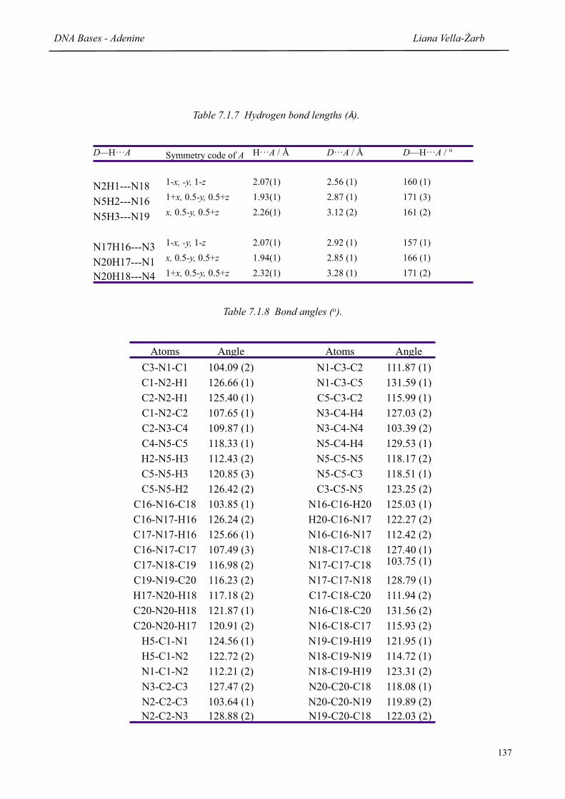
Table 7.1.7 Hydrogen bond lengths (Å).
D—H···A Symmetry code of A H···A / Å D···A / Å D—H···A / °
N2H1---N18 1-x, -y, 1-z 2.07(1) 2.56 (1) 160 (1)
N5H2---N16 1+x, 0.5-y, 0.5+z 1.93(1) 2.87 (1) 171 (3)
N5H3---N19 x, 0.5-y, 0.5+z 2.26(1) 3.12 (2) 161 (2)
N17H16---N3 1-x, -y, 1-z 2.07(1) 2.92 (1) 157 (1)
N20H17---N1 x, 0.5-y, 0.5+z 1.94(1) 2.85 (1) 166 (1)
N20H18---N4 1+x, 0.5-y, 0.5+z 2.32(1) 3.28 (1) 171 (2)
Table 7.1.8 Bond angles (o).
Atoms Angle Atoms AngleC3-N1-C1 104.09 (2) N1-C3-C2 111.87 (1)C1-N2-H1 126.66 (1) N1-C3-C5 131.59 (1)C2-N2-H1 125.40 (1) C5-C3-C2 115.99 (1)C1-N2-C2 107.65 (1) N3-C4-H4 127.03 (2)C2-N3-C4 109.87 (1) N3-C4-N4 103.39 (2)C4-N5-C5 118.33 (1) N5-C4-H4 129.53 (1)H2-N5-H3 112.43 (2) N5-C5-N5 118.17 (2)C5-N5-H3 120.85 (3) N5-C5-C3 118.51 (1)C5-N5-H2 126.42 (2) C3-C5-N5 123.25 (2)
C16-N16-C18 103.85 (1) N16-C16-H20 125.03 (1)C16-N17-H16 126.24 (2) H20-C16-N17 122.27 (2)C17-N17-H16 125.66 (1) N16-C16-N17 112.42 (2)C16-N17-C17 107.49 (3) N18-C17-C18 127.40 (1)C17-N18-C19 116.98 (2) N17-C17-C18 103.75 (1)
C19-N19-C20 116.23 (2) N17-C17-N18 128.79 (1)H17-N20-H18 117.18 (2) C17-C18-C20 111.94 (2)C20-N20-H18 121.87 (1) N16-C18-C20 131.56 (2)C20-N20-H17 120.91 (2) N16-C18-C17 115.93 (2)
H5-C1-N1 124.56 (1) N19-C19-H19 121.95 (1)H5-C1-N2 122.72 (2) N18-C19-N19 114.72 (1)N1-C1-N2 112.21 (2) N18-C19-H19 123.31 (2)N3-C2-C3 127.47 (2) N20-C20-C18 118.08 (1)N2-C2-C3 103.64 (1) N20-C20-N19 119.89 (2)N2-C2-N3 128.88 (2) N19-C20-C18 122.03 (2)
DNA Bases - Adenine Liana Vella-Żarb
137

Table 7.1.9 Crystal data, lattice parameters for theoretical structure, LeBail and Rietveld agreement factors and final refined unit cell parameters for adenine.
Crystal data
Chemical formula C5H5N5
Space group P21/c
Theoretical Structure (cc71)
a (Å) 7.4956
b (Å) 21.8311
c (Å) 7.4854
β (o) 112.43
Volume (Å3) 1132.2
Z’ 2
LeBail
Rwp (%) 8.17
Rp (%) 6.12
χ2 1.05
Refinement
Rwp (%) 12.29
Rp (%) 10.03
χ2 1.77
RF2 (%) 27.41
Preferred orientation ratio [direction] 1.1356 [121]
No. of observations 2992
No. of parameters 100
No. of restraints 80
No. of reflections 358
Final a (Å) 7.6685 (9)
Final b (Å) 22.2006 (3)
Final c (Å) 7.6240 (9)
Final β (o) 112.892 (6)
Final volume (Å3) 1195.7 (4)
DNA Bases - Adenine Liana Vella-Żarb
138

Intensity
2θ /d
egre
es
-500500
1500
2500
3500
4500
5500
1015
2025
3035
4045
5055
60
Figure 7.1.14 Rietveld refinement of adenine against the D5000 room temperature data. The green line denotes the calculated powder pattern, the red dots the experimental data, and the pink line the difference
between them. Reflection positions are shown by the black dots
DNA Bases - Adenine Liana Vella-Żarb
139

7.1.4 Crystal Structure
The crystal structure of adenine contains hydrogen bonded sheets with an interlayer spacing of 3.75
Å. It contains the sheet motif (II) shown in Figure 7.1.3, in which each molecule is linked via NH---N
hydrogen bonds to three others using all strong donors and acceptors. Each molecule is bonded through
6 hydrogen bonds, donating 3 and accepting 3, and forming R (8) and R (9) motifs. Each ring of six
molecules is surrounded by six other rings, forming a honeycomb pattern [Figure 7.1.15].
(a)
(b)
DNA Bases - Adenine Liana Vella-Żarb
140
22
22

(c)
Figure 7.1.15 (a) Crystal packing of adenine, (b) sheet made of hydrogen-bonded rings forming a honeycomb pattern and (c) R (8) and R (9) motifs shown in green and violet respectively.
7.1.4.1 Single-Crystal Structure Determination
Following our work on the crystal structure determination of adenine by structure prediction and
Rietveld refinement, we were alerted by personal communication of the concurrent work being done by
Dr Andrew Bond from the University of Southern Denmark, on the single crystal structure
determination of adenine.
His studies10 using recrystallisation by slow cooling of a saturated solution in N,N-
dimethylformamide, identified adenine as having a disordered Fddd structure (a = 8.470Å, b = 12.536Å,
c = 22.297Å). The two components of disorder are related by a 2-fold rotation axis that passes through
N2 and the midpoint of C4 [Figure 7.1.16].
DNA Bases - Adenine Liana Vella-Żarb
141
22
22

Figure 7.1.16 Two components of the adenine molecule disordered about a 2-fold rotation axis passing through N1 and the midpoint of C4 and C4i. Displacement ellipsoids are shown at 50% probability for
non-H atoms.
The resulting crystal packing is a two-dimensional hydrogen-bonded layer in which the same
honeycomb pattern is formed within the layer if the disorder components are removed [Figure 7.1.17].
Close analysis of this disordered structure and our predicted/powder structure show that the ordered
structure presented earlier in this chapter can be considered as an ordered approximation of the
disordered structure, in which the structure within each layer is illustrated by our strong hydrogen-
bonded honeycomb pattern, but that there is disorder between these layers. This is demonstrated by
projection down multiple layers of the structure in which a 4-layer repeat of the ordered P21/c model
gives the same electron density as a 2-layer repeat of the disordered Fddd model.
Figure 7.1.17 A single two-dimensional hydrogen-bonded layer in the ac plane, showing all disorder components.
DNA Bases - Adenine Liana Vella-Żarb
142
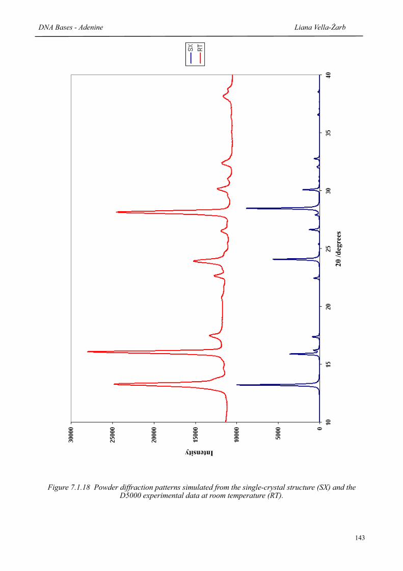
Intensity
2θ /d
egre
es
Figure 7.1.18 Powder diffraction patterns simulated from the single-crystal structure (SX) and the D5000 experimental data at room temperature (RT).
DNA Bases - Adenine Liana Vella-Żarb
143

The close relationship between these two structural models is shown by the similarity between
the experimental powder diffraction pattern used in Rietveld refinement and that simulated from the
single-crystal structure [Figure 7.1.18]. As crystal structure prediction calculations cannot generate
disordered structures, the difference between these structures is not unprecedented [Chapter 5], and is
seen as a valuable insight into the possible nature of the disorder that is observed, although further work
is needed on this aspect.
7.1.5 Low Temperature Data
Table 7.1.10 Unit cell parameters of predicted structure cc71 and from experimental data. The numbers in brackets denote the percentage change with respect to those values obtained from the 10K data.
Temperature (K) a (Å) b (Å) c (Å) β(o) Volume (Å3)
Predicted values (0K) 7.495 (1) 21.831 (1) 7.485 (2) 112.43 1132.20
10(% change)
7.539 (1)(0.00)
22.166 (2)(0.00)
7.456 (3)(0.00)
112.23(0.00)
1153.35(0.00)
50(% change)
7.533 (2)(-0.08)
22.175 (1)(+0.04)
7.537 (1)(+1.09)
111.98(-0.22)
1167.48(+1.23)
100(% change)
7.525 (1)(-0.19)
22.183 (2)(+0.08)
7.589 (2)(+1.79)
111.94(-0.26)
1175.09(+1.88)
150(% change)
7.513 (1)(-0.34)
22.235 (1)(+0.31)
0.599 (1)(+1.91)
112.14(-0.08)
1175.80(+1.95)
200(% change)
7.621 (2)(+1.09)
22.252 (2)(+0.39)
7.675 (1)(+2.94)
113.19(+0.86)
1196.27(+3.72)
250(% change)
7.628 (1)(+1.17)
22.322 (1)(+0.70)
7.714 (1)(+3.47)
113.16(+0.83)
1207.63(+4.71)
293(% change)
7.703 (1)(+2.17)
22.477 (1)(+1.40)
7.790 (2)(+4.48)
113.17(+0.84)
1239.99(+7.51)
DNA Bases - Adenine Liana Vella-Żarb
144

Since the theoretical predictions for adenine were carried out at 0K, the unit cell parameters of the
lowest energy predicted structure were used as a starting point for a LeBail fit on the 10K data. The unit
cell parameters obtained from this fit were used as a starting point for a LeBail fit on the 50K data.
Subsequent LeBail fits on the remaining temperature data sets followed the same “stepwise”
methodology [Table 7.1.10]. The powder diffraction pattern indicates a clear contraction in the unit cell
with decreasing temperature, as indicated by the shift in position of peak (112) to an increase in 2θ
[Figure 7.1.19]. The effect of changing temperature over the entire diffraction pattern from 10 to 40
degrees along 2θ is shown in Appendix A5.1.2.
2 θ / degrees
Inte
nsity
Figure 7.1.19 Section of superimposed powder diffraction data at all temperatures showing selected
peak (112) shifting towards the right with decreasing temperature. The predicted structure (cc71) is indicated by the red dotted line.
DNA Bases - Adenine Liana Vella-Żarb
145

The relatively poor crystallinity of this material (compared to other compounds studied in this
thesis) is illustrated by the broader peaks in the experimental data shown in figure 7.1.19. This can
often also be an indication of disordered components in the structure.
% c
hang
e
Temperature (K)
Figure 7.1.20 Graph showing the percentage change in unit cell dimensions with temperature.
The percentage differences in a, b, c, β and volume with varying temperature were calculated and
show an overall increase in volume with temperature [Table 7.1.10]. Although generally, a, b, c and β
also increased, there were minor fluctuations over the temperature range studied [Figure 7.1.20].
7.1.6 Discussion
The crystal structure of adenine was successfully solved using a combination of experimental data
and computational predictions. Rwp was yet again too sensitive to the inherent shift in 2θ that arises due
to the very nature of the comparison, and was therefore unsuccessful in identifying the correct structure.
This was verified by visual comparison of the powder patterns obtained experimentally against the
respective simulated patterns of the structures ranked first for each temperature [Appendix A5.1.3].
Although PolySNAP selected structure cc71 at all temperatures, the simulated powder pattern was
visually compared to the experimental patterns to verify the similarity. Simulated patterns of the
DNA Bases - Adenine Liana Vella-Żarb
146

structures ranked second at each temperature were also visually compared with the respective
experimental patterns to substantiate the initial results. Successful refinement confirmed this further.
Although Compare.x selected the wrong structure at room temperature, the correct structure was
identified at all other temperatures, providing sufficient evidence in support of structure cc71. Analysis
of the correlation results obtained with Compare.x over the range of triangle windows [Appendix
A5.1.4] shows a predominance of structure cc71 for temperatures between 10K and 250K.
Following the visual and numerical verification of the correct structure, subsequent refinement,
and discussions with Dr. Bond, adenine was found to be disordered. This is a feature that cannot be
factored into computational predictions, and it remains to be deduced experimentally. It is also what
possibly contributed to the broadening of peaks in the experimental powder patterns - and what made
initial indexing impossible. Therefore in such cases, the combination of computational predictions with
experimentally obtained powder data provides a means to overcoming these problems.
DNA Bases - Adenine Liana Vella-Żarb
147

7.2 Guanine
Figure 7.2.1 Guanine (2-amino-1,7-dihydro-6H-purin-6-one); 2-amino-6-oxypurine
7.2.1 Background
Guanine is another organic base belonging to the purine family, and it is one of the major
constituents of nucleic acids. When combined with the sugar ribose in a glycosidic linkage, guanine
forms a derivative called guanosine (a nucleoside) which in turn can be phosphorylated with from one to
three phosphoric acid groups, yielding the three nucleotides GMP (guanosine monophosphate), GDP
(guanosine diphosphate), and GTP (guanosine triphosphate). Analogous nucleosides and nucleotides
are formed from guanine and the sugar deoxyribose.
The nucleotide derivatives of guanine perform important functions in cellular metabolism. GTP acts
as a coenzyme in carbohydrate metabolism and in the biosynthesis of proteins; it can readily donate one
of its phosphate groups to adenosine diphosphate (ADP) to form adenosine triphosphate (ATP), an
extremely important derivative of adenine that acts as an intermediate in the transfer of chemical energy
in living systems. GTP is the source of guanosine found in RNA and deoxyguanosine triphosphate
(dGTP) is the source of deoxyguanosine in DNA. Thus guanine is intimately involved in the
preservation and transfer of genetic information
Prior to the commencement of this study, the crystal structure of guanine had not yet been
characterised, but related structures such as the monohydrate11 have been published.
DNA Bases - Guanine Liana Vella-Żarb
148

7.2.1.1 Experimental Polymorph Search7
An extensive polymorph search was carried out using a range of solvents, and crystallisations were
mainly carried out by slow evaporation. The majority of solvents gave either guanine derivatives, or
small particles of solid that were unsuitable for characterisation purposes.
7.2.1.2 Computational Polymorph Searches
Guanine contains both a six and a five-membered ring, along with an amine and a carbonyl group.
At the time that the initial computational predictions were carried out, there was no crystal structure
published for guanine. The most closely-related structure available was guanine monohydrate11, in
which the amino group is approximately coplanar with the ring (H-N-C-N 171.27o). For this reason, the
initial searches were carried out using a planar molecular model. These calculations resulted in 22
unique structures lying within 7 kJ mol-1 of the global lattice energy minimum. The lowest energy
hypothetical structures all consisted of three-dimensional hydrogen bond networks in which the
carbonyl oxygen acts as a hydrogen bond acceptor.
The publication of the low temperature single crystal structure of guanine (120K) by Guille and
Clegg12 in 2006 led to the decision to carry out additional computational searches, in which three
possible tautomers were considered. The original tautomer that was used in the initial search was
derived from the monohydrate structure and corresponds to tautomer 39. The published single crystal
structure was found to contain tautomer 17, while a search on another possible tautomer (tautomer 19)
was also carried out for completion. [Figure 7.2.2]
TAUTOMER 39 TAUTOMER 17 TAUTOMER 19 (initial search) (published single crystal) (hypothetical)
Figure 7.2.2 The three tautomers for guanine.
DNA Bases - Guanine Liana Vella-Żarb
149
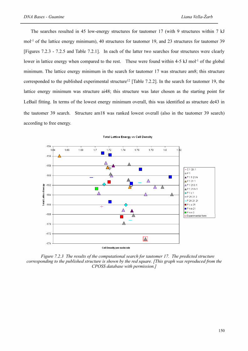
The searches resulted in 45 low-energy structures for tautomer 17 (with 9 structures within 7 kJ
mol-1 of the lattice energy minimum), 40 structures for tautomer 19, and 23 structures for tautomer 39
[Figures 7.2.3 - 7.2.5 and Table 7.2.1]. In each of the latter two searches four structures were clearly
lower in lattice energy when compared to the rest. These were found within 4-5 kJ mol-1 of the global
minimum. The lattice energy minimum in the search for tautomer 17 was structure am8; this structure
corresponded to the published experimental structure12 [Table 7.2.2]. In the search for tautomer 19, the
lattice energy minimum was structure ai48; this structure was later chosen as the starting point for
LeBail fitting. In terms of the lowest energy minimum overall, this was identified as structure de43 in
the tautomer 39 search. Structure am18 was ranked lowest overall (also in the tautomer 39 search)
according to free energy.
Figure 7.2.3 The results of the computational search for tautomer 17. The predicted structure corresponding to the published structure is shown by the red square. [This graph was reproduced from the
CPOSS database with permission.]
DNA Bases - Guanine Liana Vella-Żarb
150

Figure 7.2.4 The results of the computational search for tautomer 19. [This graph was reproduced from the CPOSS database with permission.]
Figure 7.2.5 The results of the computational search for tautomer 39. [This graph was reproduced from the CPOSS database with permission.]
DNA Bases - Guanine Liana Vella-Żarb
151

STRUCTURE SPACE GROUP
LATTICE ENERGY(kJ/mol)
FREE ENERGY(kJ/mol)
DENSITY(g/cm3)
REDUCED CELL
a(Å) b(Å) c(Å) α(°) β(°) γ(°)
Tautomer 17
am8 P 21 /n -173.03 -184.5 1.7719 3.541 9.808 16.431 90 83.166 90
am72 P 21 /n -169.75 -180.16 1.7411 8.787 9.798 10.796 90 38.336 90
aq10 P 212121 -169.19 -169.19 1.7504 17.23 9.865 3.3734 90 90 90
cd44* P c a 21 -168.48 -180.123 1.738 9.788 6.502 18.151 90 90 90
am1 P 21 /n -168.14 -180.655 1.7549 3.767 18.25 8.4544 90 79.84 90
cd25* P 21 /n -167.22 -179.3 1.7527 18.58 6.261 9.8485 90 90 89.99
am12 P 21 /c -167.11 -179.4 1.7404 3.474 9.639 19.101 90 115.599 90
dd94 C 2/c -166.37 -176.22 1.7094 9.77 9.839 12.97 90 70.388 90
cd49* P c -166.07 -166.07 1.7441 18.58 9.845 6.4459 90 77.559 90
Tautomer 19
ai48 P 21 /c -169.22 -181.566 1.7366 3.466 9.63 17.332 90 92.269 90
am101 P 21 /n -166.33 -176.809 1.7498 4.292 16.18 8.4036 90 79.362 90
ai83 P 21 /c -166.31 -166.31 1.7324 3.565 16.59 10.112 90 75.709 90
cb24* P c a 21 -166.2 -176.787 1.7296 16.18 10.07 7.1285 90 90 90
am63 P 21 /c -163.86 -176.044 1.7087 3.586 9.542 17.245 90 84.519 90
Tautomer 39
de43 C 2/c -179.32 -188.424 1.7375 12.43 7.465 19.408 90 39.922 90
ai79 P 21 /c -177.64 -188.241 1.7015 7.061 7.391 12.7 90 117.105 90
de87 C 2/c -176.36 -186.641 1.6168 13.3 6.786 14.162 90 76.31 90
am18 P 21 /n -175.86 -189.538 1.674 3.693 11.27 15.949 90 64.602 90
aq91 P 212121 -172.35 -185.481 1.6639 13.92 11.46 3.7833 90 90 90
Table 7.2.1 The low energy crystal structures (found within a maximum of 7 kJ mol-1) of the global lattice energy minimum in the computational searches for the three tautomers. Structures marked * have Z=8 (Z'=2), while all the rest have Z=4 (Z'=1).
DNA Bases - Guanine Liana Vella-Żarb
152

Table 7.2.2 Unit cell parameters of the published single crystal structure and the corresponding predicted structure for tautomer 17.
Structure a (Å) b (Å) c (Å) β (o) Volume (Å3) Space Group
Published Values12 (120K) 3.553(16) 9.693(4) 16.345(7) 95.148(6) 560.1(4) P21/c
am8 (0K) 3.541 9.808 16.431 83.17 566.6 P21/n
7.2.2 Results
When powder data were collected for guanine, the single crystal structure had not been published
yet. As it was an unknown crystal structure, the room temperature data were indexed by the DICVOL13
program on the basis of the first nineteen lines [Appendix A5.2.2]. A monoclinic cell resulted, and this
was found to be closely-related to structure ai48, the lowest energy structure from the search for
tautomer 19. The powder pattern of ai48 was simulated for visual comparison with the experimental
powder pattern [Figure 7.2.6], and a LeBail fit was done on the indexed data. [Figure 7.2.7, Table 7.2.3]
Table 7.2.3 Unit cell parameters of the predicted structure ai48, those obtained from the Le Bail fit and the index results.
Structure a (Å) b (Å) c (Å) β (o) Volume (Å3) Space Group
ai48 (0K) 3.466 9.630 17.332 92.27 578.03 P 21 /c
LeBail 3.449 8.652 18.644 99.67 548.37 P 21 /c
Index Results 3.442 8.660 18.687 99.59 549.31 P 21 /c
Additional powder data were obtained from Toni Llinas (Department of Chemistry, University of
Cambridge) and these were included in subsequent comparisons, both visual and automated. Subtle
differences were observed between these data, the single crystal simulated pattern, and the experimental
pattern [Figure 7.2.8]. In the experimental pattern, the range of peaks at positions 20-22o and the peak
at 29.5o along 2θ appear in Llinas’ data, but do not have single crystal counterparts. In addition, the peak at
43.5o on the experimental pattern does not appear in either of the other two patterns. This suggests that
although the three structures are clearly related, Llinas’ data appears to be a mixture of the other two.
DNA Bases - Guanine Liana Vella-Żarb
153

Intensity
2 θ
/ deg
rees
Figure 7.2.6 Powder diffraction pattern of predicted structure ai48 and the experimental data at room temperature (D5000).
DNA Bases - Guanine Liana Vella-Żarb
154
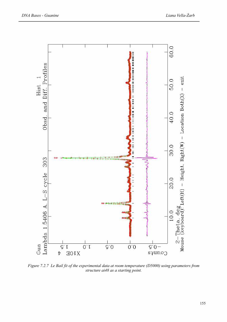
Figure 7.2.7 Le Bail fit of the experimental data at room temperature (D5000) using parameters from structure ai48 as a starting point.
DNA Bases - Guanine Liana Vella-Żarb
155

Figure 7.2.8 (a) Powder diffraction patterns of the single crystal structure, Toni Llinas’ structure and the experimental data at room temperature (full range in 2θ).
DNA Bases - Guanine Liana Vella-Żarb
156
Intensity
2 θ
/ deg
rees
0
5000
10000
15000
20000
25000
30000
35000
40000
45000
50000
5
10
15
20
25
30
35
40
45
EX
P
Sxta
l
To
ni
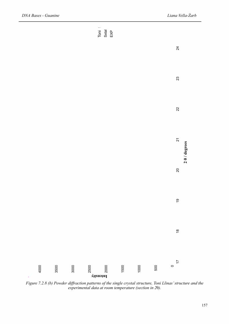
Figure 7.2.8 (b) Powder diffraction patterns of the single crystal structure, Toni Llinas’ structure and the experimental data at room temperature (section in 2θ).
DNA Bases - Guanine Liana Vella-Żarb
157
0
500
1000
1500
2000
2500
3000
3500
4000 1
7
18
19
20
21
22
23
24
#R
EF
!
Sxta
l
EX
P
Toni
Intensity
2 θ
/ deg
rees

7.2.2.1 PolySNAP
PolySNAP analysis was carried out using all seven experimental data sets (from 10K to 293K), Toni
Llinas’ data and that simulated from the single crystal structure, against all the structures predicted for
the three tautomers [Figures 7.2.9-7.2.14]. The powder diffraction pattern simulated from the single
crystal structure gave the highest correlation with that simulated from structure am8; the lowest energy
structure in the computational search for tautomer 17. Toni Llinas’ structure was ranked as being most
similar to aq10 (tautomer 17), while our experimental data was grouped with structures dd94 and am92,
from the searches for tautomers 17 and 19 respectively. Upon visual comparison of the simulated
patterns for these structures and structure ai48 with the D5005 room temperature powder pattern, some
similarities were found between the experimental data and both dd94 and ai48 [Figure 7.2.15].
Figure 7.2.9. Dendrogram showing similarity correlation clusters for predicted tautomer 17 structures, the published structure (shown as SX), Toni Llinas’ data (shown as Toni) and experimental guanine powder
diffraction patterns over a range of temperatures.
DNA Bases - Guanine Liana Vella-Żarb
158

Figure 7.2.10. Dendrogram showing similarity correlation clusters for predicted tautomer 19 structures, the published structure (shown as SX), Toni Llinas’ data (shown as Toni) and experimental guanine powder
diffraction patterns over a range of temperatures.
Figure 7.2.11. Dendrogram showing similarity correlation clusters for predicted tautomer 39 structures, the published structure (shown as SX), Toni Llinas’ data (shown as Toni) and experimental guanine powder
diffraction patterns over a range of temperatures.
DNA Bases - Guanine Liana Vella-Żarb
159

Figure 7.2.12 Correlation coefficients of all predicted structures for tautomer 17 at each experimental temperature and against the published structure (SX) and Toni Llinas’ data (Toni)
DNA Bases - Guanine Liana Vella-Żarb
160
Correlation
Stru
ctur
e
-0.1
0
0.1
0.2
0.3
0.4
0.5
0.6
0.7
0.8
0.9
10K
50K
100K
150K
200K
250K
293K
SX
To
ni
am4am12am18am26am30am60am8aq25aq36aq44av7av57av69av103aw69aw72am1am80am32am47am51am65am72am75am93ap30aq10ar33av12av16av59av85cb66cb92cb93cb100cd25cd44cd49cd59cd70cd76cd122ce40dd84dd94

-0.1
5
-0.0
5
0.0
5
0.1
5
0.2
5
0.3
5
0.4
5
0.5
5
10
K
50
K
10
0K
15
0K
20
0K
25
0K
29
3K
SX
To
ni
Correlation
Stru
ctur
e
ai48ai83ak53am71am83am92ap51av20av48ay97cb65cb86ai76aj70am10am16am31am63am87am101am112ap40ap65av73bf53cb24cb111cb133cc13cc51cd56cd60cd70cd81cd91ce44ce84fa19fa55fa64
Figure 7.2.13 Correlation coefficients of all predicted structures for tautomer 19 at each experimental temperature and against the published structure (SX) and Toni Llinas’ data (Toni)
DNA Bases - Guanine Liana Vella-Żarb
161

Correlation
Stru
ctur
e
ab49
ab72
ah5
ai9
ai36
ai79
ai95
ak70
ak75
am12
am18
am104
am105
aq91
av8
av50
az106
ba11
da53
de43
de87
fa25
fc6
-0.2
-0.1
0
0.1
0.2
0.3
0.4
10K
50K
100K
150K
200K
250K
293K
SX
To
ni
Figure 7.2.14 Correlation coefficients of all predicted structures for tautomer 39 at each experimental temperature and against the published structure (SX) and Toni Llinas’ structure (Toni)
DNA Bases - Guanine Liana Vella-Żarb
162

Intensity
2 θ
/ deg
rees
Figure 7.2.15 Powder diffraction patterns of predicted structures dd94, am92 and ai48 and the D5000 experimental structure at room temperature.
DNA Bases - Guanine Liana Vella-Żarb
163
In all cases, low temperature data were once again classed together (denoted in red in the
dendrograms). Within this cluster, the three lower temperature data sets (10K, 50K and 100K) bore the
highest correlation to one another. In the comparison for tautomer 17 [Figure 7.2.9], the three
experimental data sets were placed in separate clusters (ours in red, the published data in orange and
Llinas’ in green), though raising the cut-off point from its arbitrary position of 0.47 would see Llinas’
data being grouped with the published structure. The tautomer 19 comparison [Figure 7.2.10] grouped
the published structure and Llinas’ data in the same cluster (denoted in purple), while in the comparison
for tautomer 39, our data was grouped with Llinas’ (red), and the published data was grouped separately
(in green) [Figure 7.2.11]. Raising the cut-off point for the latter would lead to all three data sets being
grouped together. The fact that PolySNAP comparisons employ PCA for classification of structure
patterns [Chapter 2.1.2] justifies the experimental structures being classified differently for each
tautomer comparison. This is primarily because clustering of experimental patterns by this method
depends greatly on the structure patterns with which they are being compared.
7.2.3 Low Temperature Data
Using the unit cell parameters from the Le Bail fit on the D5000 data, a Le Bail fit was done on the
room temperature reflection geometry data. The unit cell parameters obtained from this fit were then
used as a starting point for fitting the data obtained at 250K. Subsequent Le Bail fits were carried out
on the remaining data collected over a range of temperatures, using the same methodology [Table 7.2.4].
As expected, there is a clear contraction of the unit cell with decreasing temperature. This is shown by
the marked decrease in volume, and the steady decrease in a and b with temperature. In order to accomodate
this change in volume, c and β fluctuate accordingly. The percentage differences in a, b, c, β and volume
with varying temperature with respect to the 10K data were calculated [Figure 7.2.16]. The contraction in the
unit cell with decreasing temperature can also be observed in the powder diffraction patterns, as indicated by
the shift in position of peak (111) to a higher 2θ value as lower temperatures are reached [Figure 7.2.17].
The effect of changing temperature over the entire diffraction pattern from 10 to 50 degrees along 2θ is
shown in Appendix A5.2.1.
DNA Bases - Guanine Liana Vella-Żarb
164

Structure a (Å) b (Å) c (Å) β (o) Volume (Å3)
Published values (120K) 3.553 9.693 16.345 95.148 560.1
D5000 (after index) 3.469 8.652 18.644 99.67 548.37
10(% change)
3.2001(0.00)
8.2581(0.00)
18.2816(0.00)
96.86(0.00)
479.67(0.00)
50(% change)
3.3500(+4.68)
8.2405(-0.21)
18.2365(-0.25)
96.22(-0.66)
500.48(+4.34)
100(% change)
3.3743(+5.44)
8.3385(+0.97)
18.4346(+0.84)
96.33(-0.55)
515.52(+7.47)
150(% change)
3.3926(+6.02)
8.5169(+3.13)
18.3957(+0.62)
97.37(+0.53)
527.14(+9.90)
200(% change)
3.4097(+6.55)
8.5319(+3.32)
18.5333(+1.38)
97.04(+0.19)
535.08(+11.55)
250(% change)
3.4380(+7.43)
8.5546(+3.59)
18.5477(+1.46)
97.36(+0.52)
540.99(+12.78)
293(% change)
3.4531(+7.91)
8.6123(+4.29)
18.5236(+1.32)
97.27(+0.42)
546.46(+13.92)
293 (D5000) 3.4486(+7.77)
8.6517(+4.77)
18.6439(+1.98)
99.66(+2.89)
548.37(+14.32)
Table 7.2.4 Unit cell parameters of published structure and those obtained from the LeBail fit on the D5000 and D5005 experimental data over a range of temperatures. The numbers in brackets denote
the percentage change with respect to those values obtained from the 10K data.
DNA Bases - Guanine Liana Vella-Żarb
165
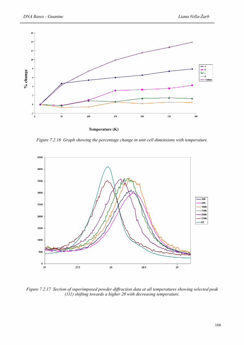
% c
hang
e
Temperature (K)
Figure 7.2.16 Graph showing the percentage change in unit cell dimensions with temperature.
Figure 7.2.17 Section of superimposed powder diffraction data at all temperatures showing selected peak (111) shifting towards a higher 2θ with decreasing temperature.
DNA Bases - Guanine Liana Vella-Żarb
166

7.2.4 Discussion
Figure 7.2.18 DNA monomer showing guanine as tautomer 19. [Figure reproduced from D. J. Taylor, N. P O. Green and G. W. Stout, “Biological Science 1 & 2”, Cambridge University Press, 3rd Edition, 1997]
Although the crystal structure of tautomer 19 has not been previously documented, its existence in nature
is certain. A detailed examination of the structure of DNA reveals that in order for guanine to form hydrogen
bonds with cytosine, thus enabling the formation of the double-helical structure characteristic of this nucleic
acid, the purine must exist as tautomer 19, with hydrogen atoms attached to N1 and N9. The possible
existence of polymorphs of this structure is not to be excluded. However, the lowest energy structures
resulting from the computational search for this tautomer all exhibited the same hydrogen bonding motif.
This implies that, although possible, the chances of the occurrence of a thermodynamically stable structure
having a different arrangement are rather remote.
DNA Bases - Guanine Liana Vella-Żarb
167

7.3 Adenine vs Guanine
Figure 7.3.1 Crystal structure of guanine12. Hydrogen bonds are shown by the green dotted lines.
The crystal structure of guanine12 contains hydrogen bonded sheets which are comparable to
those found in adenine [Section 7.1]. However, the presence of a carbonyl group in guanine is
responsible for differences in the hydrogen bonding networks of the two purines. As opposed to having
only NH----N hydrogen bonds, each molecule in guanine is linked via four NH---N and four NH---O
hydrogen bonds to three others using all strong donors and acceptors. Every molecule is bonded
through 8 hydrogen bonds, donating 4 and accepting 4, and forming R (8) and R (10) motifs. Each
ring of six molecules is again surrounded by six other rings, forming a honeycomb pattern in much the
same way as adenine does [Figures 7.3.1 and 7.3.2].
DNA Bases - Guanine Liana Vella-Żarb
168
22
22

Figure 7.3.2 Crystal structure of adenine. Hydrogen bonds are shown by the purple dotted lines.
Although the crystal structures of adenine and guanine are comparable, there are some
fundamental differences between them. While adenine has two molecules in the asymmetric unit,
guanine has only one. Their graph sets, both made up of two rings each having a pair of donors and a
pair of acceptors, follow R (8) and R (9) motifs in adenine, and R (8) and R (10) motifs in guanine.
Additionally, adenine is a disordered structure, while guanine is not.
DNA Bases - Guanine Liana Vella-Żarb
169
22
22
22
22

7.4 References
1. S. Fuji, K. Kawasaki, A. Sato, T. Fujiwara and K.-I. Tomita, Archives of Biochemistry and Biophysics, 1977, 181, 363
2. A. Takénaka and Y. Sasada, Bull. Chem. Soc. Jpn., 1982, 55, 680-686
3. M. A. Serra, B. K. Dorner and M E Silver, Acta Cryst. C, 1992, 48, 1957-1960
4. V. Langer and K. Huml, Acta Cryst. C, 1984, 40, 2080-2082
5. S. M. Tretyak, V. V. Mitkevich and L. F. Sukhodub, Kristallografiya, (SoV. Phys. Crystallogr.), 1987, 32, 1268-1271 (748-750)
6. A. C. M. Young and J. C. Dewan, Acta Cryst. C, 1991, 47, 580-584
7. Thomas C. Lewis, PhD Thesis submitted at UCL, 2007
8. A C Larson and R B Von Dreele, GSAS. General Structure Analysis System, Report No. LAUR-86-748, Los Alamos National Laboratory, Los Alamos, New Mexico, USA, 1987
9. W.A. Dollase, J. Appl. Cryst., 1986, 19, 267
10. Liana Vella-Zarb, Maryjane Tremayne, Andrew D Bond, Tom C Lewis, Derek A Tocher and Sarah L Price, 2008 (in preparation)
11. U. Thewalt, C. E. Bugg and R. E. Marsh, Acta Cryst. C, 1971, 27, 2358
12. K. Guille and W. Clegg, Acta Cryst.C, 2006, 62, 515
13. A. Boultif and D. Louër, J. Appl. Cryst., 1991, 24, 987
DNA Bases - Guanine Liana Vella-Żarb
170

8. CONCLUSIONS AND FURTHER WORK
If various polymorphic forms of an active pharmaceutical ingredient exhibit different physico-
chemical properties, characteristics such as bioavailability and toxicity may be affected. It is
primarily for this reason that during the pre-formulation stage of drug development, polymorph
screening is a time and resource-consuming, but essential process. Before a drug is launched on
the market, pharmaceutical companies apply for patents on various aspects of the drug product to
prevent others from marketing the same product. Patenting all solid forms of a drug substance
does not only protect the company that has invested money on researching that drug, but it also
serves as an assurance to patients that the relevant polymorph screens have been carried out. This
reduces the likelihood of drug substances changing form (to a potentially lethal or ineffective
form) on the shelf - a phenomenon that has proven fatal to some patients in the past. The
development of a high-throughput combinatorial strategy by which new polymorphs may be
predicted and confirmed experimentally may therefore eventually lead to the controlled
production of desired polymorphs, thus saving time and money, and reducing the risk of
Ritonavir® repetitions.
For combined techniques such as the one adopted in this project to be effective, an agreement
factor which is more reliable than Rwp is necessary for the comparison of theoretical and
experimental structures. From the study of the three known structures imidazole, chlorothalonil
and 5-azauracil described in this report, the respective Rwp values showed no agreement between
predicted and experimental structures, neither at 0K or the temperatures at which potentials were
derived, nor at temperatures corresponding to the experimental single crystal structures used for
reference. In all three cases, however, the predicted structures are correct.
The nature of the comparison made in this study imposes inevitable discrepancies between the
two powder patterns being compared. Factors which result in peak shifts along 2θ, such as
temperature difference and experimental error among others, make a pointwise comparison such
as Rwp futile, even in the case of two matching structures. More contemporary comparison
techniques such as those employed by PolySNAP and Compare allow more flexibility. Although
in the study of the three known structures neither PolySNAP nor Compare.x identified the correct
Conclusions and Further Work Liana Vella-Żarb
171

structure at all temperatures, there was reasonable overlap in all three cases. Compare.x generally
gave higher correlation values, possibly due to triangular windows encompassing more than one
peak on the corresponding powder pattern.
The inclusion of neighbourhood weighting factors (such as those used in Compare.x) leads to
a more discriminatory comparison between powder patterns, when compared with conventional
pointwise approaches. In the case of experimentally-obtained powder data, factors such as zero
point errors, preferred orientation, peak broadening, and noise may influence the outcome of the
comparison. PolySNAP comparisons, based on a principal component analysis system, search for
distinct patterns within the structures, thus overcoming some of the problems associated with
comparing experimental and theoretical data. The degree of discrimination between structures
ranked first and the next best ones was greater than that obtained during Compare.x analysis.
Again, this is probably due to the presence of more than one peak in the stipulated search window.
PolySNAP showed a greater sensitivity to temperature as opposed to Compare.x, which
demonstrated more stability across the temperature range. This could lead to a slight difference in
application of the two methods. Although there is generally an appreciable overlap of the results
obtained with both approaches, Compare.x would be the method of choice if there is a
considerable but non-definable zero-point error. If the error can be measured, then this could be
defined in PolySNAP prior to comparison. On the other hand, the presence of experimental
factors such as noise, broad peaks or preferred orientation would make PolySNAP the method of
choice.
It is clear from this study that automated comparisons are useful in enabling both the solution
of crystal structures from non-ideal powder data as well as the identification of the most likely
predicted structure out of a group of low-energy structures. Human input, however, still remains
crucial to the successful outcome of such comparisons, because while automated comparisons
reduce analysis time drastically, no two structure solution stories are identical. Numerical criteria
provided by the automated comparisons are important for the assessment of the fit in quantitative
detail. These must always, however, be complemented by graphical criteria which are essential
for visual comparison of the structures which, numerically, have resulted as best-fitting. This step
Conclusions and Further Work Liana Vella-Żarb
172

still remains crucial in any success story, because it is usually by looking at the global picture that
early noting of errors or omissions may be made.
In future, a closer look at thermal expansion and its implications could possibly be translated
into numerical form in order to be incorporated into automated comparison calculations. This
would be done in view to standardise the methods, thus making them more reproducible and
applicable to most small molecules.
Conclusions and Further Work Liana Vella-Żarb
173

9. APPENDICES
A1. Rwp
c Rwp code
program im
implicit double precision (a-h/o-z) integer natom character*10 line1 character*70 line2 character*4 line3 character*6 atom_label character*12 line4 character*68 line5 character*60 res character*18 resnam real aa,bb,cc,alpha,beta,gamma real atom_type,xx,yy,zz dimension atom_label(100),atom_type(100),xx(100),yy(100),zz(100)
OPEN (UNIT=15,STATUS='unknown',FILE='2IMIDB.EXP') OPEN (UNIT=l,STATUS='unknown',FILE='MIXU.EXP') OPEN (UNIT=21,STATUS = 'unknown',FILE='rwpval.txt') OPEN (UNIT=12,STATUS = 'unknown',FILE='rwp.txt')
c This section asks how many atoms are included in the molecule
30 WRITE (*,*) 'How many atoms are present?' READ (*,*) natom
c This part askes which res file to use
40 WRITE (*,*) 'Enter res file to use' READ (*,*) res
41 OPEN (UNIT=16,FILE=res,FORM='formatted' ,STATUS='old')
c This section reads in a,b,c,alpha,beta,gamma from the res file
98 READ (16,400,END=103) LINE3 if (line3.eq. 'TITL') GOTO 99 GOTO 98
103 continue
99 READ (16,300) AA,BB,CC,ALPHA,BETA,GAMMA
Appendix A1 Liana Vella-Żarb
174
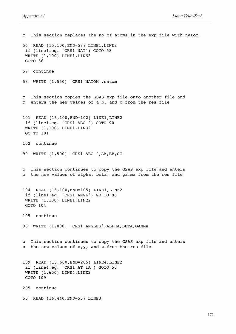
c This section replaces the no of atoms in the exp file with natom
56 READ (15,100,END=58) LINE1,LINE2 if (line1.eq. 'CRS1 NAT') GOTO 58 WRITE (1,100) LINE1,LINE2 GOTO 56
57 continue
58 WRITE (1,550) 'CRS1 NATOM',natom
c This section copies the GSAS exp file onto another file and c enters the new values of a,b, and c from the res file
101 READ (15,100,END=102) LINE1,LINE2 if (line1.eq. 'CRS1 ABC ') GOTO 90 WRITE (1,100) LINE1,LINE2 GO TO 101
102 continue
90 WRITE (1,500) 'CRS1 ABC ',AA,BB,CC
c This section continues to copy the GSAS exp file and enters c the new values of alpha, beta, and gamma from the res file
104 READ (15,100,END=105) LINE1,LINE2 if (line1.eq. 'CRS1 ANGL') GO TO 96 WRITE (1,100) LINE1,LINE2 GOTO 104
105 continue
96 WRITE (1,800) 'CRS1 ANGLES',ALPHA,BETA,GAMMA
c This section continues to copy the GSAS exp file and enters c the new values of x,y, and z from the res file
109 READ (15,600,END=205) LINE4,LINE2 if (line4.eq. 'CRS1 AT 1A') GOTO 50 WRITE (1,600) LINE4,LINE2 GOTO 109
205 continue
50 READ (16,440,END=55) LINE3
Appendix A1 Liana Vella-Żarb
175

if (line3.eq. 'SFAC') GO TO 60 GO TO 50
55 continue
c This is a loop which copies the info from the res file for as c many atoms as stated earlier in the answer to the question asked
60 DO 70 i=l,natom
READ (16,330) atom_label(i),atom_type(i),xx(i),yy(i),zz(i)
80 WRITE (1,220) 'CRS1 AT ',(i),'A','N',xx(i),yy(i),zz(i), 1 'l.000000',atom_label(i),'4 000' WRITE (1,110) 'CRS1 AT ',(i),'B','0.02500','I'
70 continue
c This section continues to copy the GSAS exp file to the end
107 READ (15,100,END=108) LINE1,LINE2 if (line1.eq. 'CRS1 AT') GOTO 107 if (line1.eq. 'CRS1 CELV') GOTO 118
118 WRITE (1,100) LINE1,LINE2
108 continue
129 READ (15,100,END=119) LINE1,LINE2 WRITE (1,100) LINE1,LINE2
40 GOTO 129
119 continue
C This section will call gsas to convert new exp file to correct c format then it will call gsas, run genles and generate a LST file
18 call system('/home/gsas/exe/cnvfile MIXU.EXP')
31 continue
32 call system('/home/gsas/exe/powpref MIXU') call system('/home/gsas/exe/genles MIXU >gsas.out') call system('rm MIXU.LST') call system('grep totals gsas.out > rwp.txt')
continue
Appendix A1 Liana Vella-Żarb
176

c This will read the rwp values and write them and res name to c rwpval.out
33 READ (12,880,end=35)rwp GOTO 33
35 rwp=rwp*100
39 continue
36 WRITE (21,900)res,rwp close (12) return continue
100 format (A10,A70) 200 format (A10,3f9.6) 300 format (8x,6f10.4) 400 format (A4,A4,A60) 500 format (A12,3f10.6) 600 format (A12,A68) 700 format (A12,A5) 800 format (A12,3f10.5) 900 format (A18,f7.4) 110 format (A10,I1,A1,2x,A7,A54) 220 format (A10,I1,A1,A3,7x,3f10.6,A10,A6,A10) 330 format (A6,A2,3f13.8) 440 format (A4,A4,A60) 550 format (A12,3x,I2,A63) 880 format (36x,f6.4)
510 stop
end
Appendix A1 Liana Vella-Żarb
177

A2. IMIDAZOLE
A2.1 Low Temperature Data
Figure A2.1 Powder diffraction data at all temperatures (D5005)
Appendix A2 Liana Vella-Żarb
178
Intensity
2 θ
/ deg
rees
0
20000
40000
60000
80000
100000
120000 1
0
15
20
25
30
35
40
10K
50K
150K
200K
250K
RT

A2.2 Rwp
!"
#!!!"
$!!!!"
$#!!!"
%!!!!"
%#!!!"
&!!!!"
$!"
$#"
%!"
%#"
&!"
&#"
'!"
'#"
#!"
()*$"
$!+"
Intensity
2 θ
/ deg
rees
Figure A2.2.1 Powder pattern of top ranked predicted structure at 10K (D5005) and experimental pattern at that temperature
Appendix A2 Liana Vella-Żarb
179

Intensity
2 θ
/ deg
rees
!"
#!!!"
$!!!!"
$#!!!"
%!!!!"
%#!!!"
&!!!!"
&#!!!"
'!!!!"
$!"
$#"
%!"
%#"
&!"
&#"
'!"
()&'"
#!*"
Figure A2.2.2 Powder pattern of top ranked predicted structure at 50K (D5005) and experimental pattern at that temperature
Appendix A2 Liana Vella-Żarb
180

Intensity
2 θ
/ deg
rees
!"
#!!!"
$!!!!"
$#!!!"
%!!!!"
%#!!!"
&!!!!"
&#!!!"
'!!!!"
'#!!!"
#!!!!" $!"
$#"
%!"
%#"
&!"
&#"
'!"
%#!("
$#!("
)*&#"
Figure A2.2.3 Powder pattern of top ranked predicted structure at 150K and 250K (D5005) and experimental patterns at these temperatures
Appendix A2 Liana Vella-Żarb
181

!"
#!!!"
$!!!!"
$#!!!"
%!!!!"
%#!!!"
&!!!!"
&#!!!" $!"
$#"
%!"
%#"
&!"
&#"
'!"
'#"
#!"
%!!("
)*&+"
Intensity
2 θ
/ deg
rees
Figure A2.2.4 Powder pattern of top ranked predicted structure at 200K (D5005) and experimental pattern at that temperature
Appendix A2 Liana Vella-Żarb
182

Intensity
2 θ
/ deg
rees
!"
#!!!"
$!!!!"
$#!!!"
%!!!!"
%#!!!"
&!!!!"
$!"
$#"
%!"
%#"
&!"
&#"
'!"
()"
*+&,"
Figure A2.2.5 Powder pattern of top ranked predicted structure at room temperature (D5005) and experimental pattern at that temperature
Appendix A2 Liana Vella-Żarb
183

!"
#!!!"
$!!!!"
$#!!!"
%!!!!"
%#!!!"
&!!!!" $!"
$#"
%!"
%#"
&!"
&#"
'!"
%(&)"*+#!!!,"
-.''"
Intensity
2 θ
/ deg
rees
Figure A2.2.6 Powder pattern of top ranked predicted structure at room temperature (D5000) and experimental pattern at that temperature
Appendix A2 Liana Vella-Żarb
184

A2.3 PolySNAP
0
5000
10000
15000
20000
25000
30000
35000
40000
45000
50000 1
0
15
20
25
30
35
40
10K
50K
am
32
2 θ
/ deg
rees
Intensity
Figure A2.3.1 Powder pattern of top ranked predicted structure at 10K and 50K (D5005), and experimental patterns at those temperatures
Appendix A2 Liana Vella-Żarb
185

Intensity
2 θ
/ deg
rees
!"
#!!!!"
$!!!!"
%!!!!"
&!!!!"
'!!!!"
(!!!!"
)!!!!"
*!!!!"
+!!!!" #!"
#'"
$!"
$'"
%!"
%'"
&!"
$!!,"
$'!,"
#'!,"
-."
/0%&"
Figure A2.3.2 Powder patterns of top ranked predicted structure at 150K, 200K, 250K and room temperature (D5005) and experimental patterns at those temperatures
Appendix A2 Liana Vella-Żarb
186

!"
#!!!"
$!!!!"
$#!!!"
%!!!!"
%#!!!"
&!!!!" $!"
$#"
%!"
%#"
&!"
&#"
'!"
%(&)"*+#!!!,"
-.&#"
Intensity
2 θ
/ deg
rees
Figure A2.3.3 Powder patterns of top ranked predicted structure at room temperature (D5000) and experimental patterns at those temperatures
Appendix A2 Liana Vella-Żarb
187

A2.4 Compare.x
0
5000
10000
15000
20000
25000
30000
35000
40000
45000
50000 1
0
15
20
25
30
35
40
10K
50K
am
32
2 θ
/ deg
rees
Intensity
Figure A2.4.1 Powder pattern of top ranked predicted structure at 10K and 50K (D5005) and experimental patterns at those temperatures
Appendix A2 Liana Vella-Żarb
188
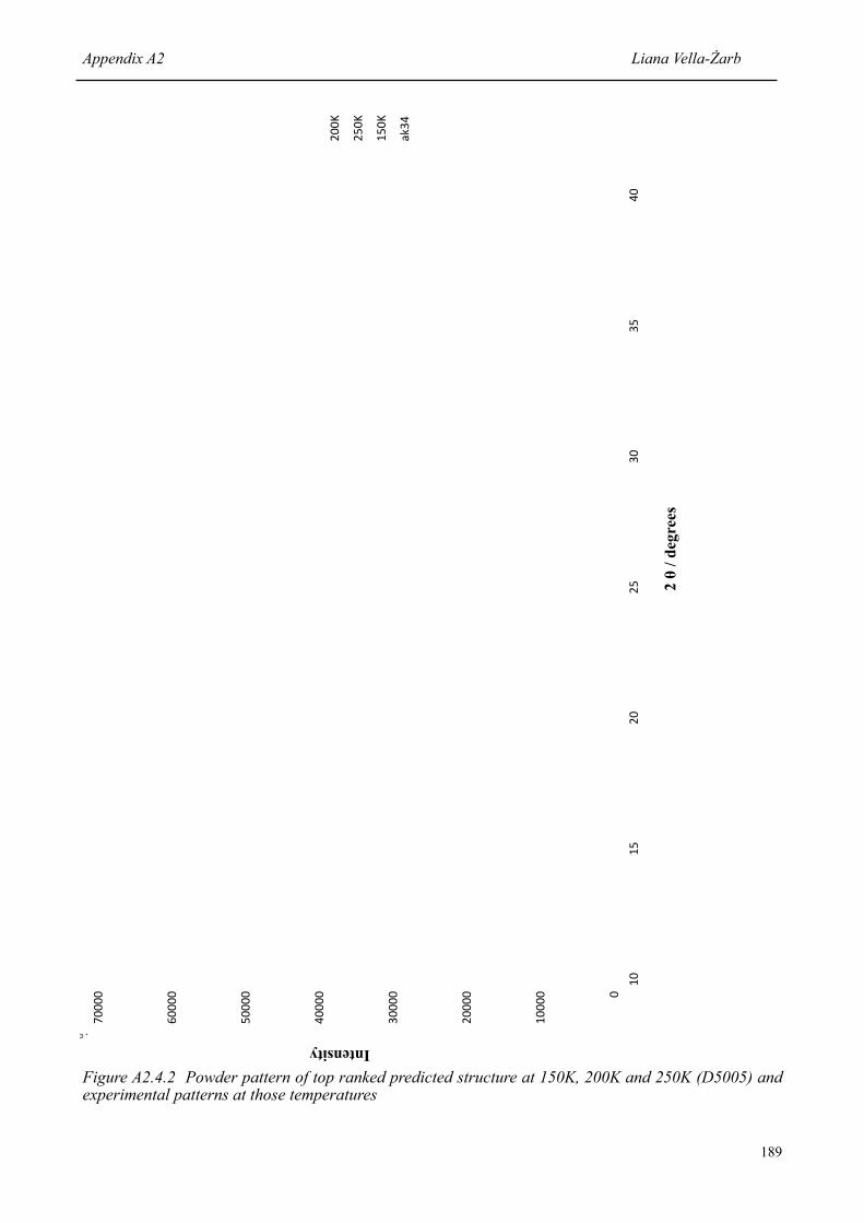
Intensity
2 θ
/ deg
rees
!"
#!!!!"
$!!!!"
%!!!!"
&!!!!"
'!!!!"
(!!!!"
)!!!!" #!"
#'"
$!"
$'"
%!"
%'"
&!"
$!!*"
$'!*"
#'!*"
+,%&"
Figure A2.4.2 Powder pattern of top ranked predicted structure at 150K, 200K and 250K (D5005) and experimental patterns at those temperatures
Appendix A2 Liana Vella-Żarb
189

Intensity
2 θ
/ deg
rees
!"
#!!!"
$!!!!"
$#!!!"
%!!!!"
%#!!!"
&!!!!"
&#!!!"
'!!!!"
'#!!!" $!"
$#"
%!"
%#"
&!"
&#"
'!"
'#"
%(&)"*+#!!!,"
-.&#"
%(&)"*+#!!#,"
Figure A2.4.3 Powder pattern of top ranked predicted structure at room temperature (D5000 and D5005) and experimental patterns at those temperatures
Appendix A2 Liana Vella-Żarb
190

Results obtained using Compare.x with various values of triangle windows. In each case, the tables
show the structure with the highest correlation coefficient [C(x)] at each temperature, and the difference
to the value obtained for the correct structure [C(ak34)]. In cases where the correct structure was
identified, the difference was positive. An incorrect match gave a negative difference, as shown by the
values in red and blue. Blue denotes ak34 being ranked second, while values in red correspond to ak34
being ranked third or lower.
Table A2.4.1. Triangle window 0.5.
Temperature (K) Structure Correlation Coefficient Difference[C(ak34) - C(x)]
10
50
150
200
250
293
293 (D5000)
am32 0.66294 -0.19810
am32 0.67067 -0.17771
ak66 0.73371 -0.07523
ak66 0.76105 -0.06888
ak34 0.76115 0.01505
ai35 0.71675 -0.12950
ai35 0.65683 -0.19758
Table A2.4.2. Triangle window 1.0.
Temperature (K) Structure Correlation Coefficient Difference[C(ak34) - C(x)]
10
50
150
200
250
293
293 (D5000)
am32 0.76926 -0.12467
am32 0.78164 -0.11389
ak66 0.83363 -0.02332
ak66 0.83856 -0.00668
ak34 0.87510 0.03544
ai35 0.81807 -0.06026
ai35 0.77485 -0.10092
Appendix A2 Liana Vella-Żarb
191

Table A2.4.3. Triangle window 1.5.
Temperature (K) Structure Correlation Coefficient Difference[C(ak34) - C(x)]
10
50
150
200
250
293
293 (D5000)
am32 0.83533 -0.08420
am32 0.84838 -0.07779
ak66 0.86600 -0.00920
ak66 0.86577 -0.00446
ak34 0.88965 0.00686
ai35 0.86348 -0.03613
ai35 0.85226 -0.07900
Table A2.4.4. Triangle window 2.0.
Temperature (K) Structure Correlation Coefficient Difference[C(ak34) - C(x)]
10
50
150
200
250
293
293 (D5000)
am32 0.86910 -0.05156
am32 0.87991 -0.04717
ak34 0.89473 0.00721
ak34 0.89512 0.01275
ak34 0.90977 0.01048
ai35 0.89375 -0.03221
ai35 0.89247 -0.03365
Appendix A2 Liana Vella-Żarb
192
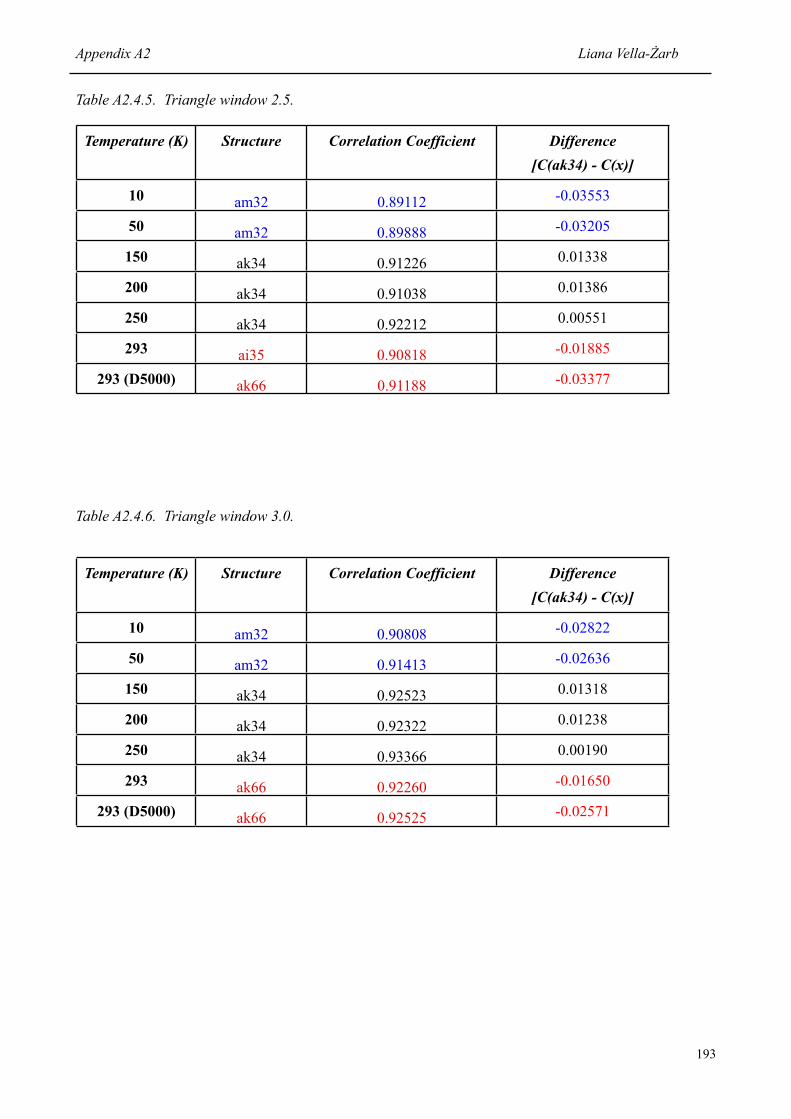
Table A2.4.5. Triangle window 2.5.
Temperature (K) Structure Correlation Coefficient Difference[C(ak34) - C(x)]
10
50
150
200
250
293
293 (D5000)
am32 0.89112 -0.03553
am32 0.89888 -0.03205
ak34 0.91226 0.01338
ak34 0.91038 0.01386
ak34 0.92212 0.00551
ai35 0.90818 -0.01885
ak66 0.91188 -0.03377
Table A2.4.6. Triangle window 3.0.
Temperature (K) Structure Correlation Coefficient Difference[C(ak34) - C(x)]
10
50
150
200
250
293
293 (D5000)
am32 0.90808 -0.02822
am32 0.91413 -0.02636
ak34 0.92523 0.01318
ak34 0.92322 0.01238
ak34 0.93366 0.00190
ak66 0.92260 -0.01650
ak66 0.92525 -0.02571
Appendix A2 Liana Vella-Żarb
193

Table A2.4.7. Triangle window 3.5.
Temperature (K) Structure Correlation Coefficient Difference[C(ak34) - C(x)]
10
50
150
200
250
293
293 (D5000)
am32 0.92110 -0.02490
am32 0.92577 -0.02319
ak34 0.93457 0.00755
ak34 0.93216 0.00494
ak66 0.94071 -0.00933
fc72 0.93305 -0.01911
ai35 0.92540 -0.01989
Table A2.4.8. Triangle window 4.0.
Temperature (K) Structure Correlation Coefficient Difference[C(ak34) - C(x)]
10
50
150
200
250
293
293 (D5000)
am32 0.93231 -0.02221
am32 0.93623 -0.02051
ak34 0.94255 0.00220
ak34 0.93948 0.00132
ak66 0.94588 -0.00222
fc72 0.94320 -0.02327
ai35 0.92926 -0.01748
Appendix A2 Liana Vella-Żarb
194

A3. CHLOROTHALONIL
A3.1 Low Temperature Data
Figure A3.1 Powder diffraction data at all temperatures (D5005)
Appendix A3 Liana Vella-Żarb
195
2 θ
/ deg
rees
Intensity
0
200
400
600
800
1000
1200
1400
1600
1800 1
0
15
20
25
30
35
40
45
10
0K
15
0K
20
0K
25
0K
29
3K

A3.2 Rwp
Intensity
2 θ
/ deg
rees
!"
#!!"
$!!"
%!!"
&!!"
'!!"
(!!"
)!!"
*!!"
+!!"
#!"
#'"
$!"
$'"
%!"
%'"
&!"
#!!,"
$+%,"
-.#+"
Figure A3.2.1 Powder pattern of top ranked predicted structure at 100K and room temperature (D5005) and experimental patterns at these temperatures
Appendix A3 Liana Vella-Żarb
196

Intensity
2 θ
/ deg
rees
!"
#!!"
$!!"
%!!"
&!!"
'!!"
(!!"
)!!" #!"
#'"
$!"
$'"
%!"
%'"
&!"
&'"
'!"
''"
(!"
#'!*"
+,#%"
Figure A3.2.2 Powder pattern of top ranked predicted structure at 150K (D5005) and experimental pattern at that temperature
Appendix A3 Liana Vella-Żarb
197

Intensity
2 θ
/ deg
rees
!"
#!!"
$!!"
%!!"
&!!"
'!!"
(!!"
)!!" #!"
#'"
$!"
$'"
%!"
%'"
&!"
&'"
'!"
''"
(!"
$!!*"
+,&)"
Figure A3.2.3 Powder pattern of top ranked predicted structure at 200K (D5005) and experimental pattern at that temperature
Appendix A3 Liana Vella-Żarb
198
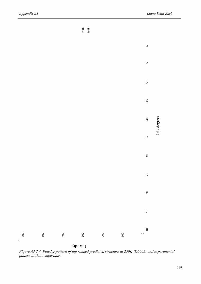
Intensity
2 θ
/ deg
rees
!"
#!!"
$!!"
%!!"
&!!"
'!!"
(!!" #!"
#'"
$!"
$'"
%!"
%'"
&!"
&'"
'!"
''"
(!"
$'!)"
*+&,"
Figure A3.2.4 Powder pattern of top ranked predicted structure at 250K (D5005) and experimental pattern at that temperature
Appendix A3 Liana Vella-Żarb
199
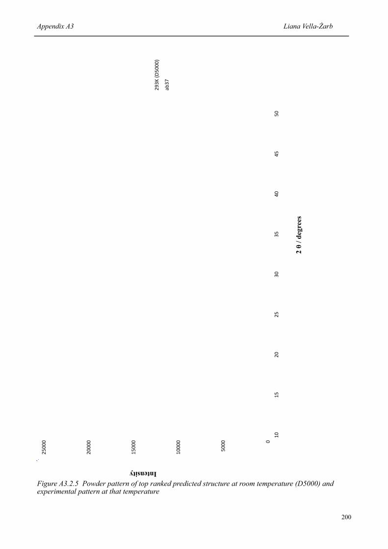
Intensity
2 θ
/ deg
rees
!"
#!!!"
$!!!!"
$#!!!"
%!!!!"
%#!!!" $!"
$#"
%!"
%#"
&!"
&#"
'!"
'#"
#!"
%(&)"*+#!!!,"
-.&/"
Figure A3.2.5 Powder pattern of top ranked predicted structure at room temperature (D5000) and experimental pattern at that temperature
Appendix A3 Liana Vella-Żarb
200
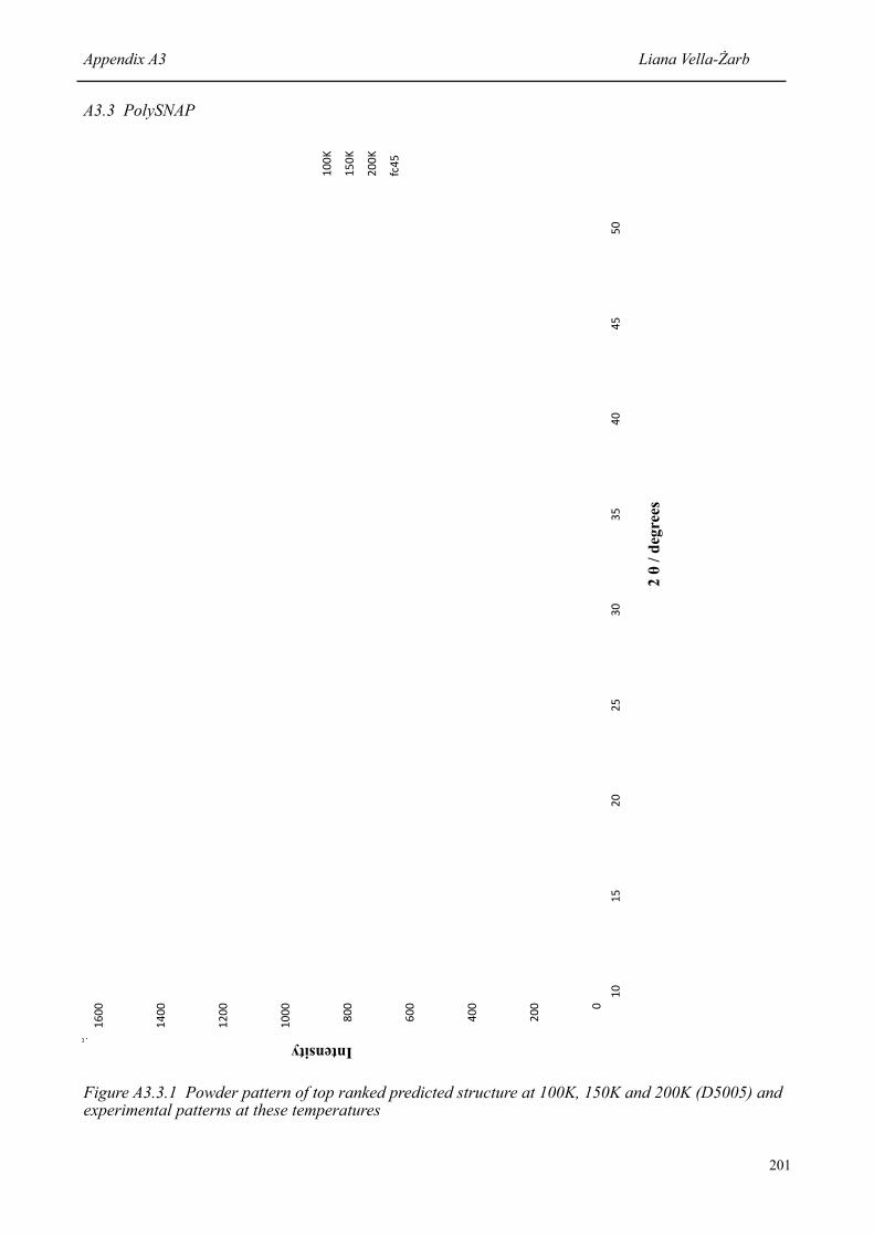
A3.3 PolySNAP
!"
#!!"
$!!"
%!!"
&!!"
'!!!"
'#!!"
'$!!"
'%!!" '!"
'("
#!"
#("
)!"
)("
$!"
$("
(!"
'!!*"
'(!*"
#!!*"
+,$("
Intensity
2 θ
/ deg
rees
Figure A3.3.1 Powder pattern of top ranked predicted structure at 100K, 150K and 200K (D5005) and experimental patterns at these temperatures
Appendix A3 Liana Vella-Żarb
201

Intensity
2 θ
/ deg
rees
!"
#!!"
$!!"
%!!"
&!!"
'!!"
(!!"
)!!"
*!!"
+!!"
#!!!" #!"
#'"
$!"
$'"
%!"
%'"
&!"
&'"
'!"
$'!,"
$+%,"
-.&&"
Figure A3.3.2 Powder pattern of top ranked predicted structure at 250K and room temperature (D5005) and experimental patterns at these temperatures
Appendix A3 Liana Vella-Żarb
202

Intensity
2 θ
/ deg
rees
!"
#!!!"
$!!!!"
$#!!!"
%!!!!"
%#!!!" $!"
$#"
%!"
%#"
&!"
&#"
'!"
'#"
#!"
%(&)"*+#!!!,"
-.$/"
Figure A3.3.3 Powder pattern of top ranked predicted structure at room temperature (D5000) and experimental pattern at that temperature
Appendix A3 Liana Vella-Żarb
203

A3.4 Compare.x
Intensity
2 θ
/ deg
rees
!"
#!!!"
$!!!!"
$#!!!"
%!!!!"
%#!!!"
&!!!!" $!"
$#"
%!"
%#"
&!"
&#"
'!"
'#"
#!"
$!!("
)*'"
Figure A3.4.1 Powder pattern of top ranked predicted structure at 100K (D5005) and experimental pattern at that temperature
Appendix A3 Liana Vella-Żarb
204

Intensity
2 θ
/ deg
rees
!"
#!!"
$!!"
%!!"
&!!"
'!!!"
'#!!"
'$!!"
'%!!"
'&!!"
#!!!" '!"
'("
#!"
#("
)!"
)("
$!"
$("
(!"
'(!*"
#!!*"
#(!*"
+,$("
Figure A3.4.2 Powder pattern of top ranked predicted structure at 150K, 200K and 250K (D5005) and experimental patterns at these temperatures
Appendix A3 Liana Vella-Żarb
205

Intensity
2 θ
/ deg
rees
!"
#!!!"
$!!!!"
$#!!!"
%!!!!"
%#!!!"
&!!!!"
&#!!!"
'!!!!" $!"
$#"
%!"
%#"
&!"
&#"
'!"
'#"
#!"
%(&)"*+#!!!,"
%(&)"*+#!!#,"
-.'/"
Figure A3.4.3 Powder pattern of top ranked predicted structure at room temperature (D5000 and D5005) and experimental pattern at that temperature
Appendix A3 Liana Vella-Żarb
206

Results obtained using Compare.x with various values of triangle windows. In each case, the tables
show the structure with the highest correlation coefficient [C(x)] at each temperature, and the difference
to the value obtained for the correct structure [C(fc45)]. In cases where the correct structure was
identified, the difference was positive. An incorrect match gave a negative difference, as shown by the
values in red and blue. Blue denotes fc45 being ranked second, while values in red correspond to fc45
being ranked third or lower.
Table A3.4.1. Triangle window 0.5.
Temperature (K) Structure Correlation Coefficient Difference[C(fc45) - C(x)]
100
150
200
250
293
293 (D5000)
fc45 0.82539 0.03170
fc45 0.85025 0.08551
fc45 0.85246 0.09692
fc45 0.81109 0.01029
ai44 0.83041 -0.07613
fc47 0.50190 -0.05690
Table A3.4.2. Triangle window 1.0.
Temperature (K) Structure Correlation Coefficient Difference[C(fc45) - C(x)]
100
150
200
250
293
293 (D5000)
fc4 0.88291 -0.00194
fc45 0.88761 0.01623
fc45 0.88579 0.03166
fc45 0.87166 0.00510
fc47 0.87741 -0.02883
fc47 0.61438 -0.07702
Appendix A3 Liana Vella-Żarb
207
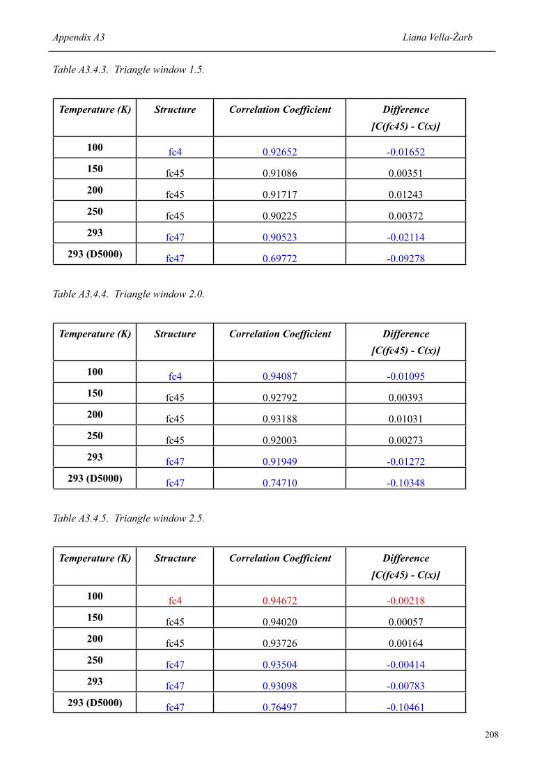
Table A3.4.3. Triangle window 1.5.
Temperature (K) Structure Correlation Coefficient Difference[C(fc45) - C(x)]
100
150
200
250
293
293 (D5000)
fc4 0.92652 -0.01652
fc45 0.91086 0.00351
fc45 0.91717 0.01243
fc45 0.90225 0.00372
fc47 0.90523 -0.02114
fc47 0.69772 -0.09278
Table A3.4.4. Triangle window 2.0.
Temperature (K) Structure Correlation Coefficient Difference[C(fc45) - C(x)]
100
150
200
250
293
293 (D5000)
fc4 0.94087 -0.01095
fc45 0.92792 0.00393
fc45 0.93188 0.01031
fc45 0.92003 0.00273
fc47 0.91949 -0.01272
fc47 0.74710 -0.10348
Table A3.4.5. Triangle window 2.5.
Temperature (K) Structure Correlation Coefficient Difference[C(fc45) - C(x)]
100
150
200
250
293
293 (D5000)
fc4 0.94672 -0.00218
fc45 0.94020 0.00057
fc45 0.93726 0.00164
fc47 0.93504 -0.00414
fc47 0.93098 -0.00783
fc47 0.76497 -0.10461
Appendix A3 Liana Vella-Żarb
208

Table A3.4.6. Triangle window 3.0.
Temperature (K) Structure Correlation Coefficient Difference[C(fc45) - C(x)]
100
150
200
250
293
293 (D5000)
fc4 0.95481 -0.00317
fc45 0.94662 0.00024
fc45 0.94161 0.00242
fc47 0.93676 -0.00025
fc47 0.93356 -0.00475
fc47 0.77165 -0.08863
Table A3.4.7. Triangle window 3.5.
Temperature (K) Structure Correlation Coefficient Difference[C(fc45) - C(x)]
100
150
200
250
293
293 (D5000)
fc4 0.96368 -0.00686
fc4 0.95494 -0.00385
fc4 0.94846 -0.00232
fc47 0.94264 -0.00045
fc47 0.93894 -0.00442
fc47 0.78153 -0.10575
Table A3.4.8. Triangle window 4.0.
Temperature (K) Structure Correlation Coefficient Difference[C(fc45) - C(x)]
100
150
200
250
293
293 (D5000)
fc4 0.96980 -0.00759
fc4 0.96079 -0.00474
fc4 0.95493 -0.00387
fc4 0.94900 -0.00282
fc4 0.94372 -0.00349
fc4 0.79224 -0.11128
Appendix A3 Liana Vella-Żarb
209

A4. 5-AZAURACIL
A4.1 Low Temperature Data
0
20
00
0
40
00
0
60
00
0
80
00
0
10
00
00
10
1
5
20
2
5
30
3
5
40
10K
100K
150K
200K
250K
293K
2 θ
/ deg
rees
Intensity
Figure A4.1 Powder diffraction data at all temperatures (D5005)
Appendix A4 Liana Vella-Żarb
210

A4.2 Rwp
Intensity
2 θ
/ deg
rees
!"
#!!!"
$!!!!"
$#!!!"
%!!!!"
%#!!!"
&!!!!" $!"
$#"
%!"
%#"
&!"
&#"
'!"
$!("
)*+%"
Figure A4.2.1 Powder pattern of top ranked predicted structure at 10K (D5005) and experimental pattern at that temperature
Appendix A4 Liana Vella-Żarb
211

Intensity
2 θ
/ deg
rees
!"
#!!!"
$!!!!"
$#!!!"
%!!!!"
%#!!!"
&!!!!"
$!"
$#"
%!"
%#"
&!"
&#"
'!"
$!!("
)*+,"
Figure A4.2.2 Powder pattern of top ranked predicted structure at 100K (D5005) and experimental pattern at that temperature
Appendix A4 Liana Vella-Żarb
212

!"
#!!!"
$!!!!"
$#!!!"
%!!!!"
%#!!!"
&!!!!" $!"
$#"
%!"
%#"
&!"
&#"
'!"
$#!("
)*+#"
Intensity
2 θ
/ deg
rees
Figure A4.2.3 Powder pattern of top ranked predicted structure at 150K (D5005) and experimental pattern at that temperature
Appendix A4 Liana Vella-Żarb
213

Intensity
2 θ
/ deg
rees
!"
#!!!"
$!!!!"
$#!!!"
%!!!!"
%#!!!"
&!!!!"
$!"
$#"
%!"
%#"
&!"
&#"
'!"
%!!("
)*+,"
Figure A4.2.4 Powder pattern of top ranked predicted structure at 200K (D5005) and experimental pattern at that temperature
Appendix A4 Liana Vella-Żarb
214

Intensity
2 θ
/ deg
rees
!"
#!!!"
$!!!!"
$#!!!"
%!!!!"
%#!!!"
&!!!!" $!"
$#"
%!"
%#"
&!"
&#"
'!"
%#!("
)*#$"
Figure A4.2.5 Powder pattern of top ranked predicted structure at 250K (D5005) and experimental pattern at that temperature
Appendix A4 Liana Vella-Żarb
215

Intensity
2 θ
/ deg
rees
!"
#!!!!"
$!!!!"
%!!!!"
&!!!!"
'!!!!"
(!!!!"
#!"
#'"
$!"
$'"
%!"
%'"
&!"
)*"
+,($"
Figure A4.2.6 Powder pattern of top ranked predicted structure at room temperature (D5005) and experimental pattern at that temperature
Appendix A4 Liana Vella-Żarb
216

Intensity
2 θ
/ deg
rees
!"
#!!!"
$!!!!"
$#!!!"
%!!!!"
%#!!!"
&!!!!" $!"
$#"
%!"
%#"
&!"
&#"
'!"
(#!!!"
)*$$+"
Figure A4.2.7 Powder pattern of top ranked predicted structure at room temperature (D5000) and experimental pattern at that temperature
Appendix A4 Liana Vella-Żarb
217
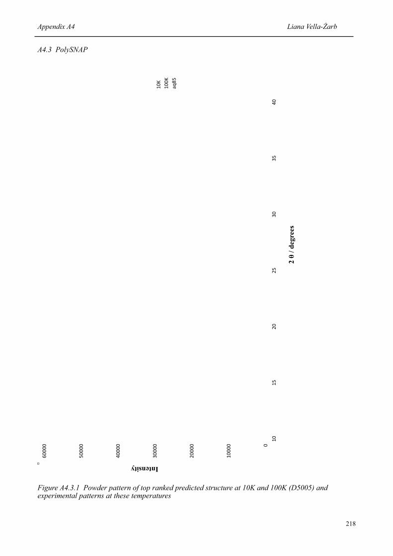
A4.3 PolySNAP
Intensity
2 θ
/ deg
rees
!"
#!!!!"
$!!!!"
%!!!!"
&!!!!"
'!!!!"
(!!!!"
#!"
#'"
$!"
$'"
%!"
%'"
&!"
#!)"
#!!)"
*+,'"
Figure A4.3.1 Powder pattern of top ranked predicted structure at 10K and 100K (D5005) and experimental patterns at these temperatures
Appendix A4 Liana Vella-Żarb
218

Intensity
2 θ
/ deg
rees
!"
#!!!!"
$!!!!"
%!!!!"
&!!!!"
'!!!!!"
'#!!!!" '!"
'("
#!"
#("
)!"
)("
$!"
'(!*"
#!!*"
#(!*"
#+)*"
,-#"
Figure A4.3.2 Powder pattern of top ranked predicted structure at 150K, 200K, 250K and room temperature (D5005) and experimental patterns at these temperatures
Appendix A4 Liana Vella-Żarb
219

Intensity
2 θ
/ deg
rees
!"
#!!!"
$!!!!"
$#!!!"
%!!!!"
%#!!!"
&!!!!" $!"
$#"
%!"
%#"
&!"
&#"
'!"
(#!!!"
)*$$+"
Figure A4.3.3 Powder pattern of top ranked predicted structure at room temperature (D5000) and experimental pattern at that temperature
Appendix A4 Liana Vella-Żarb
220

A4.4 Compare.x
Intensity
2 θ
/ deg
rees
!"
#!!!!"
$!!!!"
%!!!!"
&!!!!"
'!!!!"
(!!!!" #!"
#'"
$!"
$'"
%!"
%'"
&!"
#!)"
#!!)"
*+&#"
Figure A4.4.1 Powder pattern of top ranked predicted structure at 10K and 100K (D5005) and experimental patterns at these temperatures
Appendix A4 Liana Vella-Żarb
221

Intensity
2 θ
/ deg
rees
!"
#!!!!"
$!!!!"
%!!!!"
&!!!!"
'!!!!"
(!!!!"
)!!!!"
*!!!!" #!"
#'"
$!"
$'"
%!"
%'"
&!"
#'!+"
$!!+"
$'!+"
,-$"
Figure A4.4.2 Powder pattern of top ranked predicted structure at 150K, 200K and 250K (D5005) and experimental patterns at these temperatures
Appendix A4 Liana Vella-Żarb
222

Intensity
2 θ
/ deg
rees
!"
#!!!!"
$!!!!"
%!!!!"
&!!!!"
'!!!!"
(!!!!" #!"
#'"
$!"
$'"
%!"
%'"
&!"
)*"
+,##-"
Figure A4.4.3 Powder pattern of top ranked predicted structure at room temperature (D5005) and experimental pattern at that temperature
Appendix A4 Liana Vella-Żarb
223
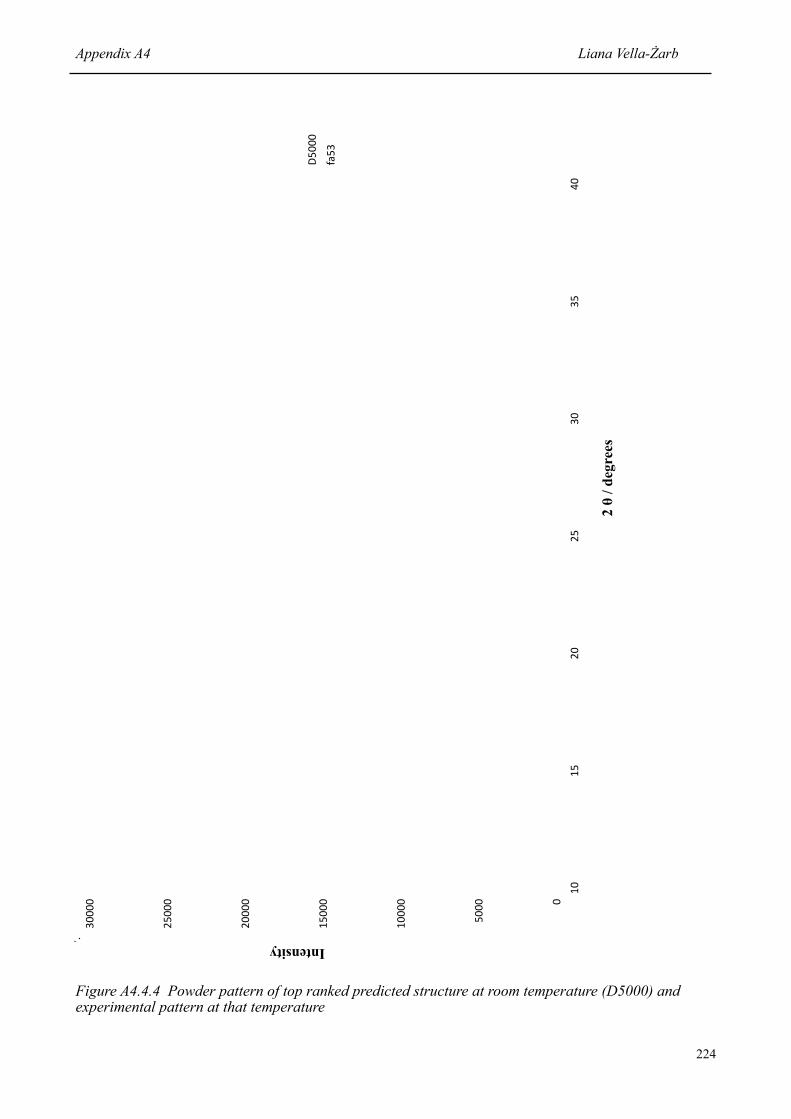
Intensity
2 θ
/ deg
rees
!"
#!!!"
$!!!!"
$#!!!"
%!!!!"
%#!!!"
&!!!!" $!"
$#"
%!"
%#"
&!"
&#"
'!"
(#!!!"
)*#&"
Figure A4.4.4 Powder pattern of top ranked predicted structure at room temperature (D5000) and experimental pattern at that temperature
Appendix A4 Liana Vella-Żarb
224

Results obtained using Compare.x with various values of triangle windows. In each case, the tables
show the structure with the highest correlation coefficient [C(x)] at each temperature, and the difference
to the value obtained for the correct structure [C(cb2)]. In cases where the correct structure was
identified, the difference was positive. An incorrect match gave a negative difference, as shown by the
values in red and blue. Blue denotes cb2 being ranked second, while values in red correspond to cb2
being ranked third or lower.
Table A4.4.1. Triangle window 0.5.
Temperature (K) Structure Correlation Coefficient Difference[C(cb2) - C(x)]
10
100
150
200
250
293
293 (D5000)
aq85 0.78135 -0.34852
aq85 0.76313 -0.27214
aq62 0.68007 -0.05562
fa22 0.70322 -0.04605
cb2 0.69752 0.00385
fc54 0.70654 -0.10698
cb117 0.57229 -0.17499
Table A4.4.2. Triangle window 1.0.
Temperature (K) Structure Correlation Coefficient Difference[C(cb2) - C(x)]
10
100
150
200
250
293
293 (D5000)
aq85 0.79499 -0.11708
aq85 0.79274 -0.08851
fa22 0.76337 -0.00333
fa22 0.77458 -0.00205
cb2 0.78864 0.00949
cb117 0.80960 -0.05846
cb117 0.63186 -0.08100
Appendix A4 Liana Vella-Żarb
225
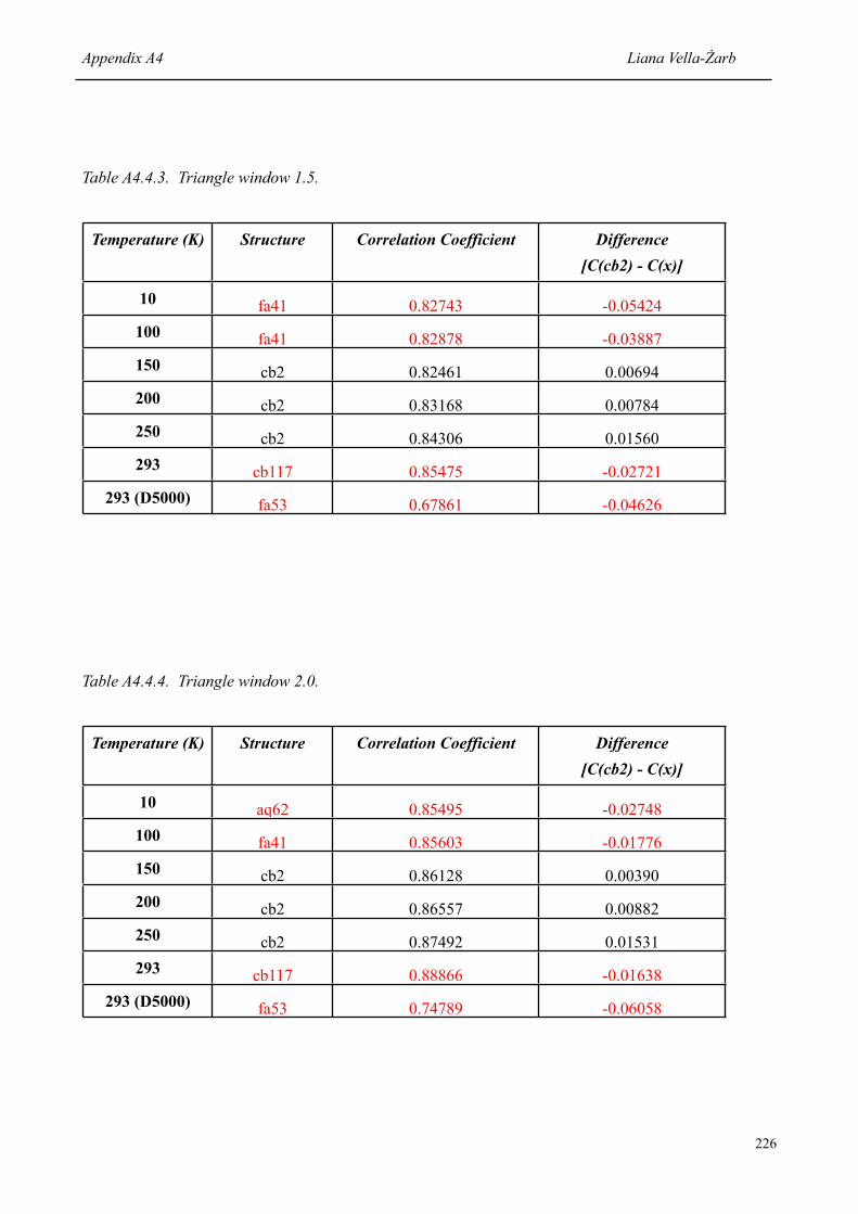
Table A4.4.3. Triangle window 1.5.
Temperature (K) Structure Correlation Coefficient Difference[C(cb2) - C(x)]
10
100
150
200
250
293
293 (D5000)
fa41 0.82743 -0.05424
fa41 0.82878 -0.03887
cb2 0.82461 0.00694
cb2 0.83168 0.00784
cb2 0.84306 0.01560
cb117 0.85475 -0.02721
fa53 0.67861 -0.04626
Table A4.4.4. Triangle window 2.0.
Temperature (K) Structure Correlation Coefficient Difference[C(cb2) - C(x)]
10
100
150
200
250
293
293 (D5000)
aq62 0.85495 -0.02748
fa41 0.85603 -0.01776
cb2 0.86128 0.00390
cb2 0.86557 0.00882
cb2 0.87492 0.01531
cb117 0.88866 -0.01638
fa53 0.74789 -0.06058
Appendix A4 Liana Vella-Żarb
226

Table A4.4.5. Triangle window 2.5.
Temperature (K) Structure Correlation Coefficient Difference[C(cb2) - C(x)]
10
100
150
200
250
293
293 (D5000)
fa41 0.87017 -0.01149
aq62 0.87444 -0.00779
cb2 0.88649 0.00438
cb2 0.89075 0.00958
cb2 0.90463 0.01662
cb2 0.91051 0.00481
fa53 0.79366 -0.06947
Table A4.4.6. Triangle window 3.0.
Temperature (K) Structure Correlation Coefficient Difference[C(cb2) - C(x)]
10
100
150
200
250
293
293 (D5000)
aq62 0.88611 -0.00688
aq62 0.89214 -0.00606
cb2 0.90135 0.00310
cb2 0.90400 0.00332
cb2 0.91328 0.00682
fc54 0.92535 -0.00629
fa53 0.81837 -0.07854
Appendix A4 Liana Vella-Żarb
227
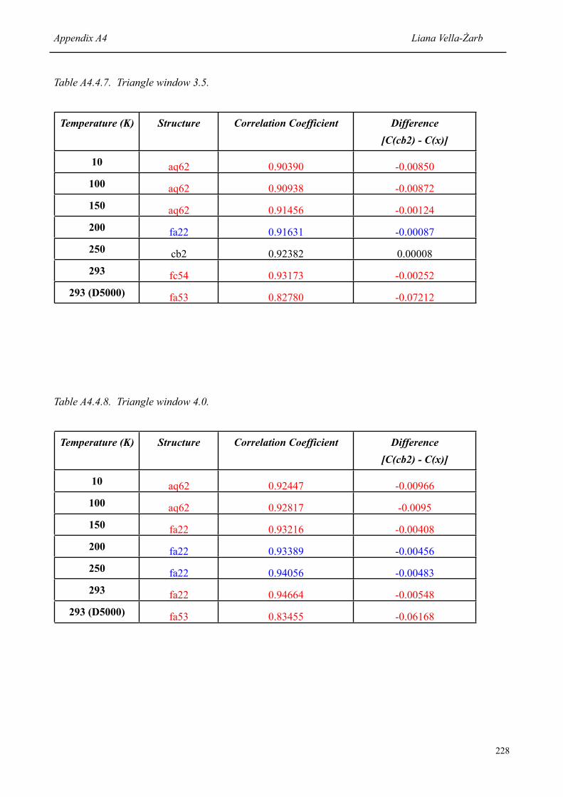
Table A4.4.7. Triangle window 3.5.
Temperature (K) Structure Correlation Coefficient Difference[C(cb2) - C(x)]
10
100
150
200
250
293
293 (D5000)
aq62 0.90390 -0.00850
aq62 0.90938 -0.00872
aq62 0.91456 -0.00124
fa22 0.91631 -0.00087
cb2 0.92382 0.00008
fc54 0.93173 -0.00252
fa53 0.82780 -0.07212
Table A4.4.8. Triangle window 4.0.
Temperature (K) Structure Correlation Coefficient Difference[C(cb2) - C(x)]
10
100
150
200
250
293
293 (D5000)
aq62 0.92447 -0.00966
aq62 0.92817 -0.0095
fa22 0.93216 -0.00408
fa22 0.93389 -0.00456
fa22 0.94056 -0.00483
fa22 0.94664 -0.00548
fa53 0.83455 -0.06168
Appendix A4 Liana Vella-Żarb
228

A5. DNA BASES
A5.1 Adenine
A5.1.1 Background
Method Solvents Results
Slow evaporation Methanol, propan-2-ol, tertbutylmethylether, THF, butan-1-ol, propan-1-ol
Small particles of solid - not enough for characterisation analysis
Slow evaporation 2,2,2-trifluoroethanol, acetic acid, dimethylamine in H2O, 2-methoxyetylamine
Microcrystalline solid - powder pattern matched stock sample
Slow evaporation 2-chloroethanol Adeninium chloride hemihydrate
Slow evaporation Equimolar amounts of thymine/adenine and cytosine/adenine in dilute hydrochloric acid, dilute h y d r o c h l o r i c a c i d , concentrated hydrochloric acid
Adeninium dichloride
Slow evaporation H2O Microcrystalline solid - poor powder pattern which could not be indexed, did not match stock sample or known trihydrate structure
Sublimation - Microcrystalline solid - powder pattern matched stock sample
Table A5.1.1 The results of the crystallisation experiments on adenine. Other crystallisation experiments did not give any products for analysis7 [Referenced on page 116].
Appendix A5 Liana Vella-Żarb
229

A5.1.1 Low Temperature Data
0
10
00
0
20
00
0
30
00
0
40
00
0
50
00
0
60
00
0 1
0
15
2
0
25
3
0
35
4
0
10
K
50
K
10
0K
15
0K
20
0K
25
0K
RT
2 θ
/ deg
rees
Intensity
Figure A5.1.1 Powder diffraction data at all temperatures (D5005)
Appendix A5 Liana Vella-Żarb
230
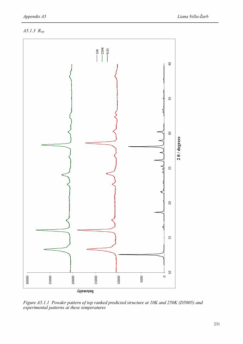
A5.1.3 Rwp
Intensity
2 θ
/ deg
rees
!"
#!!!"
$!!!!"
$#!!!"
%!!!!"
%#!!!"
&!!!!" $!"
$#"
%!"
%#"
&!"
&#"
'!"
$!("
%#!("
)*&&"
Figure A5.1.1 Powder pattern of top ranked predicted structure at 10K and 250K (D5005) and experimental patterns at these temperatures
Appendix A5 Liana Vella-Żarb
231

Intensity
2 θ
/ deg
rees
!"
#!!!"
$!!!"
%!!!"
&!!!"
'!!!!"
'#!!!"
'$!!!"
'%!!!"
'&!!!"
#!!!!" '!"
'("
#!"
#("
)!"
)("
$!"
(!*"
+,(%"
Figure A5.1.2 Powder pattern of top ranked predicted structure at 50K (D5005) and experimental pattern at this temperature
Appendix A5 Liana Vella-Żarb
232

Intensity
2 θ
/ deg
rees
!"
#!!!"
$!!!!"
$#!!!"
%!!!!"
%#!!!"
&!!!!" $!"
$#"
%!"
%#"
&!"
&#"
'!"
$!!("
%!!("
)*+,"
Figure A5.1.3 Powder pattern of top ranked predicted structure at 100K and 200K (D5005) and experimental patterns at these temperatures
Appendix A5 Liana Vella-Żarb
233
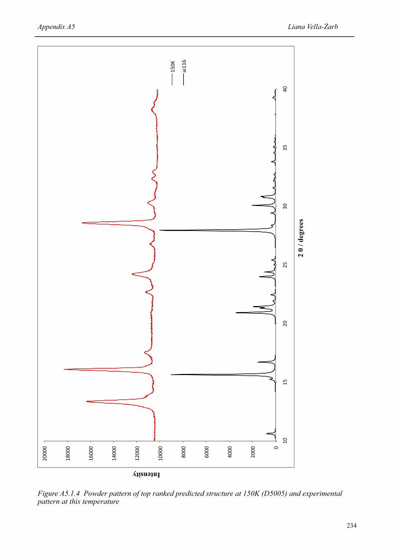
Intensity
2 θ
/ deg
rees
!"
#!!!"
$!!!"
%!!!"
&!!!"
'!!!!"
'#!!!"
'$!!!"
'%!!!"
'&!!!"
#!!!!" '!"
'("
#!"
#("
)!"
)("
$!"
'(!*"
+,''%"
Figure A5.1.4 Powder pattern of top ranked predicted structure at 150K (D5005) and experimental pattern at this temperature
Appendix A5 Liana Vella-Żarb
234

Intensity
2 θ
/ deg
rees
!"
#!!!"
$!!!"
%!!!"
&!!!"
'!!!!"
'#!!!"
'$!!!"
'%!!!"
'&!!!" '!"
'("
#!"
#("
)!"
)("
$!"
*+"
,,'!'"
Figure A5.1.5 Powder pattern of top ranked predicted structure at room temperature (D5005) and experimental pattern at this temperature
Appendix A5 Liana Vella-Żarb
235

Intensity
2 θ
/ deg
rees
!"
#!!!"
$!!!!"
$#!!!"
%!!!!"
%#!!!" $!"
$#"
%!"
%#"
&!"
&#"
'!"
(#!!!"
)*$+"
Figure A5.1.6 Powder pattern of top ranked predicted structure at room temperature (D5000) and experimental pattern at this temperature
Appendix A5 Liana Vella-Żarb
236

A5.1.4 Compare.x
Results obtained using Compare.x with various values of triangle windows. In each case, the tables
show the structure with the highest correlation coefficient [C(x)] at each temperature, and the difference
to the value obtained for the correct structure [C(cc71)]. In cases where the correct structure was
identified, the difference was positive. An incorrect match gave a negative difference, as shown by the
values in red and blue. Blue denotes cc71 being ranked second, while values in red correspond to cc71
being ranked third or lower.
Table A5.1.4.1. Triangle window 0.5.
Temperature (K) Structure Correlation Coefficient Difference[C(cc71) - C(x)]
10
50
100
150
200
250
293
293 (D5000)
fc4 0.79532 -0.32973
fc4 0.80933 -0.33646
fc4 0.7996 -0.32923
fc4 0.78255 -0.32015
fc4 0.73332 -0.2863
fc4 0.6329 -0.21183
am43 0.61454 -0.2076
am43 0.60252 -0.27965
Appendix A5 Liana Vella-Żarb
237

Table A5.1.4.2. Triangle window 1.0.
Temperature (K) Structure Correlation Coefficient Difference[C(cc71) - C(x)]
10
50
100
150
200
250
293
293 (D5000)
fc4 0.84304 -0.22984
fc4 0.85032 -0.23712
fc4 0.84302 -0.22966
fc4 0.83462 -0.22113
fc4 0.80994 -0.20158
fc4 0.76287 -0.16559
am43 0.74622 -0.16182
am43 0.6563 -0.22563
Table A5.1.4.3. Triangle window 1.5.
Temperature (K) Structure Correlation Coefficient Difference[C(cc71) - C(x)]
10
50
100
150
200
250
293
293 (D5000)
cc71 0.86323 0.10665
cc71 0.86793 0.1147
cc71 0.86202 0.11012
cc71 0.85685 0.09648
cc71 0.83976 0.07151
cc71 0.81179 0.02576
cc71 0.80019 0.02112
cc71 0.69074 0.02096
Appendix A5 Liana Vella-Żarb
238
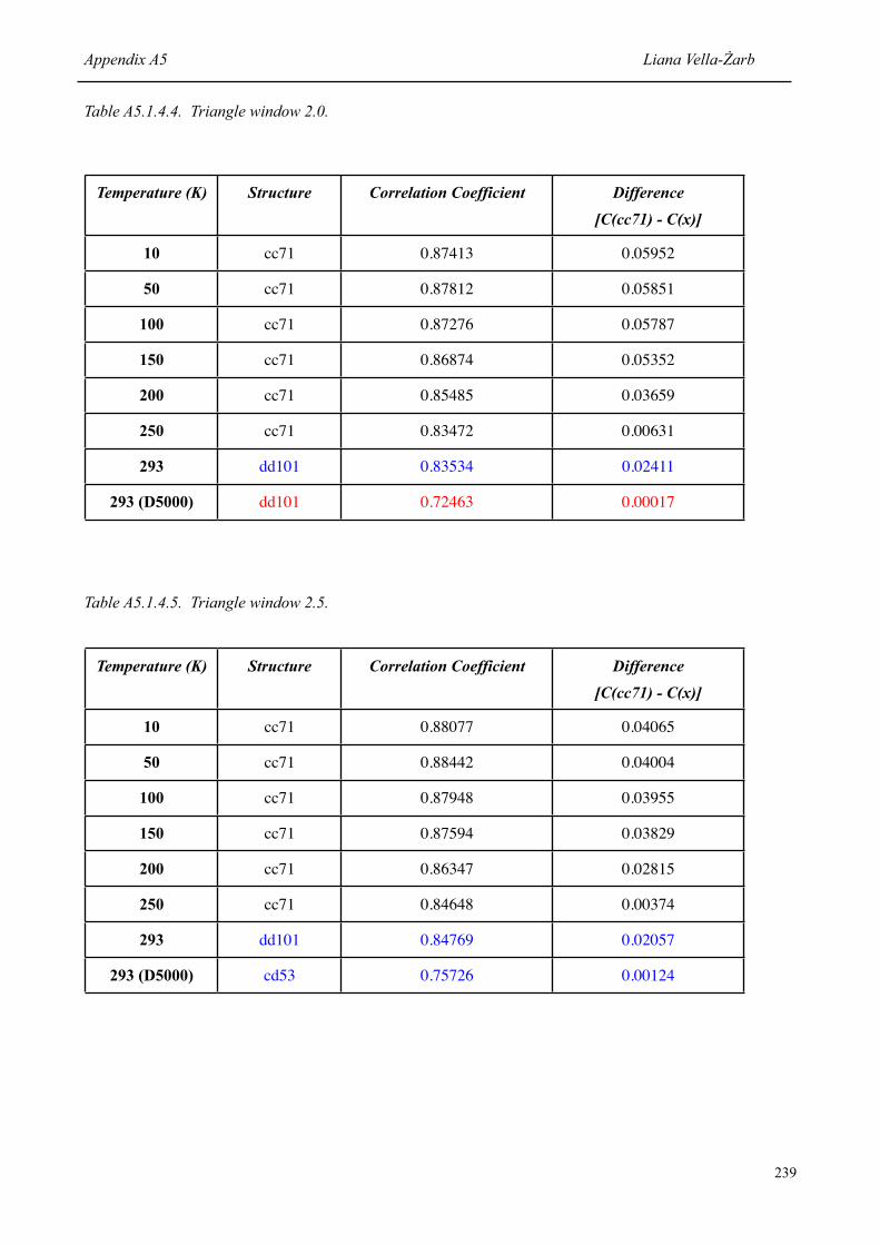
Table A5.1.4.4. Triangle window 2.0.
Temperature (K) Structure Correlation Coefficient Difference[C(cc71) - C(x)]
10
50
100
150
200
250
293
293 (D5000)
cc71 0.87413 0.05952
cc71 0.87812 0.05851
cc71 0.87276 0.05787
cc71 0.86874 0.05352
cc71 0.85485 0.03659
cc71 0.83472 0.00631
dd101 0.83534 0.02411
dd101 0.72463 0.00017
Table A5.1.4.5. Triangle window 2.5.
Temperature (K) Structure Correlation Coefficient Difference[C(cc71) - C(x)]
10
50
100
150
200
250
293
293 (D5000)
cc71 0.88077 0.04065
cc71 0.88442 0.04004
cc71 0.87948 0.03955
cc71 0.87594 0.03829
cc71 0.86347 0.02815
cc71 0.84648 0.00374
dd101 0.84769 0.02057
cd53 0.75726 0.00124
Appendix A5 Liana Vella-Żarb
239
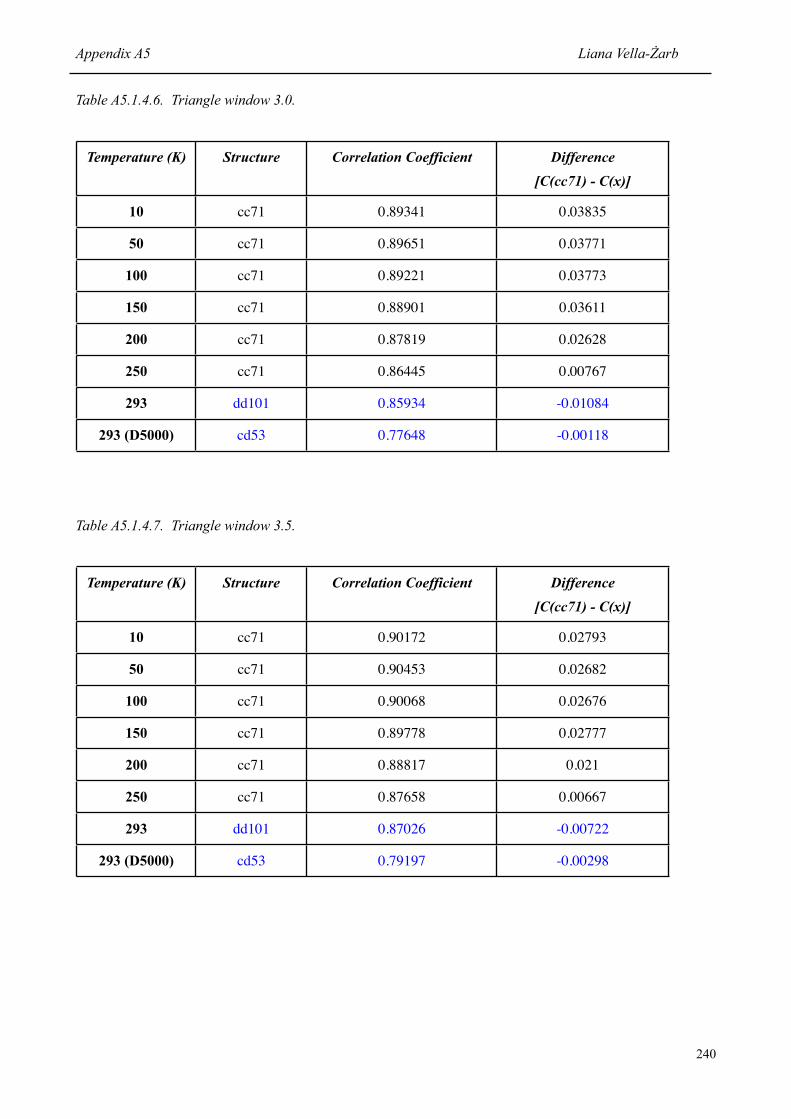
Table A5.1.4.6. Triangle window 3.0.
Temperature (K) Structure Correlation Coefficient Difference[C(cc71) - C(x)]
10
50
100
150
200
250
293
293 (D5000)
cc71 0.89341 0.03835
cc71 0.89651 0.03771
cc71 0.89221 0.03773
cc71 0.88901 0.03611
cc71 0.87819 0.02628
cc71 0.86445 0.00767
dd101 0.85934 -0.01084
cd53 0.77648 -0.00118
Table A5.1.4.7. Triangle window 3.5.
Temperature (K) Structure Correlation Coefficient Difference[C(cc71) - C(x)]
10
50
100
150
200
250
293
293 (D5000)
cc71 0.90172 0.02793
cc71 0.90453 0.02682
cc71 0.90068 0.02676
cc71 0.89778 0.02777
cc71 0.88817 0.021
cc71 0.87658 0.00667
dd101 0.87026 -0.00722
cd53 0.79197 -0.00298
Appendix A5 Liana Vella-Żarb
240

Table A5.1.4.8. Triangle window 4.0.
Temperature (K) Structure Correlation Coefficient Difference[C(cc71) - C(x)]
10
50
100
150
200
250
293
293 (D5000)
cc71 0.90983 0.01494
cc71 0.91243 0.01424
cc71 0.90887 0.01445
cc71 0.90626 0.01462
cc71 0.89769 0.01341
cc71 0.88819 0.00376
dd101 0.88282 -0.00495
cd53 0.81021 -0.00463
Appendix A5 Liana Vella-Żarb
241

A5.2 Guanine
0
5000
10000
15000
20000
25000
30000 1
0
15
20
25
30
35
40
45
50
10
K
50
K
10
0K
15
0K
20
0K
25
0K
RT
2 θ
/ deg
rees
Intensity
A5.2.1 Low Temperature Data
Appendix A5 Liana Vella-Żarb
242

A5.2.2 Guanine Indexing Output
Running summary of all solutions logged so far for this dataset name,sorted in descending order of I20 then Merit (as defined by each program)
I20 Merit Volume V/V1 BL IndexProg Date Time Pedig a b c alpha beta gamma Q(A) Q(B) Q(C) Q(D) Q(E) Q(F) Description (up to 80-chars, from Run-Title line)19 17.6 584.475 1.00 P DICVOL91/log 20Mar07 11:57:30 Mon_16 20.1396 8.6592 3.6633 90.000 113.811 90.000 29.456 133.366 890.276 .000 130.755 .000 GUANINE = guanine19 17.6 584.475 1.00 P DICVOL91/log 20Mar07 11:56:51 Mon_16 20.1396 8.6592 3.6633 90.000 113.811 90.000 29.456 133.366 890.276 .000 130.755 .000 GUANINE = guanine19 17.5 584.306 1.00 P DICVOL91/log 20Mar07 11:57:30 Mon_27 23.0636 8.6590 3.6623 90.000 126.975 90.000 29.455 133.372 1168.179 .000 223.140 .000 GUANINE = guanine19 17.5 584.306 1.00 P DICVOL91/log 20Mar07 11:56:51 Mon_27 23.0636 8.6590 3.6623 90.000 126.975 90.000 29.455 133.372 1168.179 .000 223.140 .000 GUANINE = guanine19 17.2 584.308 1.00 P DICVOL91/log 20Mar07 11:57:30 Mon_11 19.5542 8.6590 3.6623 90.000 109.562 90.000 29.455 133.372 839.716 .000 105.316 .000 GUANINE = guanine19 17.2 584.308 1.00 P DICVOL91/log 20Mar07 11:56:51 Mon_11 19.5542 8.6590 3.6623 90.000 109.562 90.000 29.455 133.372 839.716 .000 105.316 .000 GUANINE = guanine19 16.1 586.087 1.00 P DICVOL91/log 20Mar07 11:57:30 Mon_22 21.8221 8.6579 3.6739 90.000 122.397 90.000 29.455 133.406 1039.188 .000 187.475 .000 GUANINE = guanine19 16.1 586.087 1.00 P DICVOL91/log 20Mar07 11:56:51 Mon_22 21.8221 8.6579 3.6739 90.000 122.397 90.000 29.455 133.406 1039.188 .000 187.475 .000 GUANINE = guanine19 16.0 586.188 1.00 P DICVOL91/log 20Mar07 11:57:30 Mon_14 19.5976 8.6579 3.6746 90.000 109.918 90.000 29.456 133.406 837.832 .000 107.037 .000 GUANINE = guanine19 16.0 586.188 1.00 P DICVOL91/log 20Mar07 11:56:51 Mon_14 19.5976 8.6579 3.6746 90.000 109.918 90.000 29.456 133.406 837.832 .000 107.037 .000 GUANINE = guanine19 15.7 598.235 1.02 P DICVOL91/log 20Mar07 11:57:30 Mon__6 18.7431 8.6598 3.7490 90.000 100.542 90.000 29.451 133.347 736.131 .000 53.877 .000 GUANINE = guanine19 15.7 598.235 1.02 P DICVOL91/log 20Mar07 11:56:51 Mon__6 18.7431 8.6598 3.7490 90.000 100.542 90.000 29.451 133.347 736.131 .000 53.877 .000 GUANINE = guanine19 15.7 598.234 1.02 P DICVOL91/log 20Mar07 11:57:30 Mon_23 21.4230 8.6598 3.7490 90.000 120.668 90.000 29.451 133.347 961.687 .000 171.681 .000 GUANINE = guanine19 15.7 598.234 1.02 P DICVOL91/log 20Mar07 11:56:51 Mon_23 21.4230 8.6598 3.7490 90.000 120.668 90.000 29.451 133.347 961.687 .000 171.681 .000 GUANINE = guanine19 15.7 598.233 1.02 P DICVOL91/log 20Mar07 11:57:30 Mon__7 18.8705 8.6598 3.7490 90.000 102.451 90.000 29.451 133.347 746.177 .000 63.924 .000 GUANINE = guanine
Appendix A5 Liana Vella-Żarb
243

19 15.7 598.233 1.02 P DICVOL91/log 20Mar07 11:57:30 Mon_15 19.7755 8.6598 3.7490 90.000 111.284 90.000 29.451 133.347 819.465 .000 112.783 .000 GUANINE = guanine19 15.7 598.233 1.02 P DICVOL91/log 20Mar07 11:56:51 Mon__7 18.8705 8.6598 3.7490 90.000 102.451 90.000 29.451 133.347 746.177 .000 63.924 .000 GUANINE = guanine19 15.7 598.233 1.02 P DICVOL91/log 20Mar07 11:56:51 Mon_15 19.7755 8.6598 3.7490 90.000 111.284 90.000 29.451 133.347 819.465 .000 112.783 .000 GUANINE = guanine19 14.4 584.677 1.00 P DICVOL91/log 20Mar07 11:57:30 Mon_26 24.0562 8.6575 3.6635 90.000 129.977 90.000 29.427 133.418 1268.841 .000 248.294 .000 GUANINE = guanine19 14.4 584.677 1.00 P DICVOL91/log 20Mar07 11:56:51 Mon_26 24.0562 8.6575 3.6635 90.000 129.977 90.000 29.427 133.418 1268.841 .000 248.294 .000 GUANINE = guanine19 14.1 598.419 1.02 P DICVOL91/log 20Mar07 11:57:30 Mon_17 20.0158 8.6637 3.7487 90.000 112.993 90.000 29.455 133.227 839.734 .000 122.866 .000 GUANINE = guanine19 14.1 598.419 1.02 P DICVOL91/log 20Mar07 11:56:51 Mon_17 20.0158 8.6637 3.7487 90.000 112.993 90.000 29.455 133.227 839.734 .000 122.866 .000 GUANINE = guanine19 13.9 584.677 1.00 P DICVOL91/log 20Mar07 11:57:30 Mon__5 18.9674 8.6575 3.6635 90.000 103.616 90.000 29.427 133.418 788.803 .000 71.733 .000 GUANINE = guanine19 13.9 584.677 1.00 P DICVOL91/log 20Mar07 11:56:51 Mon__5 18.9674 8.6575 3.6635 90.000 103.616 90.000 29.427 133.418 788.803 .000 71.733 .000 GUANINE = guanine19 13.9 547.453 .94 P DICVOL91/log 20Mar07 11:57:30 Mon__9 9.1369 18.4244 3.4299 90.000 108.533 90.000 133.247 29.459 945.565 .000 225.646 .000 GUANINE = guanine19 13.9 547.453 .94 P DICVOL91/log 20Mar07 11:56:51 Mon__9 9.1369 18.4244 3.4299 90.000 108.533 90.000 133.247 29.459 945.565 .000 225.646 .000 GUANINE = guanine19 13.9 547.452 .94 P DICVOL91/log 20Mar07 11:57:30 Mon__1 8.6790 18.4244 3.4299 90.000 93.473 90.000 133.247 29.459 853.167 .000 40.850 .000 GUANINE = guanine19 13.9 547.452 .94 P DICVOL91/log 20Mar07 11:56:51 Mon__1 8.6790 18.4244 3.4299 90.000 93.473 90.000 133.247 29.459 853.167 .000 40.850 .000 GUANINE = guanine19 13.9 547.450 .94 P DICVOL91/log 20Mar07 11:57:30 Mon_12 9.5234 18.4244 3.4299 90.000 114.542 90.000 133.248 29.459 1027.263 .000 307.345 .000 GUANINE = guanine19 13.9 547.450 .94 P DICVOL91/log 20Mar07 11:56:51 Mon_12 9.5234 18.4244 3.4299 90.000 114.542 90.000 133.248 29.459 1027.263 .000 307.345 .000 GUANINE = guanine19 13.5 549.308 .94 P DICVOL91/log 20Mar07 11:57:30 Mon_25 22.8078 8.6603 3.4423 90.000 126.110 90.000 29.453 133.332 1293.008 .000 230.017 .000 GUANINE = guanine19 13.5 549.308 .94 P DICVOL91/log 20Mar07 11:56:51 Mon_25 22.8078 8.6603 3.4423 90.000 126.110 90.000 29.453 133.332 1293.008 .000 230.017 .000 GUANINE = guanine
Appendix A5 Liana Vella-Żarb
244
19 13.3 549.308 .94 P DICVOL91/log 20Mar07 11:57:30 Mon_20 20.9644 8.6603 3.4423 90.000 118.487 90.000 29.453 133.332 1092.442 .000 171.110 .000 GUANINE = guanine19 13.3 549.308 .94 P DICVOL91/log 20Mar07 11:56:51 Mon_20 20.9644 8.6603 3.4423 90.000 118.487 90.000 29.453 133.332 1092.442 .000 171.110 .000 GUANINE = guanine19 13.3 549.305 .94 P DICVOL91/log 20Mar07 11:57:30 Mon__3 18.6874 8.6603 3.4423 90.000 99.594 90.000 29.453 133.332 868.034 .000 53.298 .000 GUANINE = guanine19 13.3 549.305 .94 P DICVOL91/log 20Mar07 11:57:30 Mon_10 19.5579 8.6603 3.4423 90.000 109.588 90.000 29.453 133.332 950.787 .000 112.205 .000 GUANINE = guanine19 13.3 549.305 .94 P DICVOL91/log 20Mar07 11:56:51 Mon__3 18.6874 8.6603 3.4423 90.000 99.594 90.000 29.453 133.332 868.034 .000 53.298 .000 GUANINE = guanine19 13.3 549.305 .94 P DICVOL91/log 20Mar07 11:56:51 Mon_10 19.5579 8.6603 3.4423 90.000 109.588 90.000 29.453 133.332 950.787 .000 112.205 .000 GUANINE = guanine19 12.3 580.673 .99 P DICVOL91/log 20Mar07 11:57:30 Mon__8 9.0564 18.4383 3.6383 90.000 107.103 90.000 133.467 29.414 826.969 .000 195.408 .000 GUANINE = guanine19 12.3 580.673 .99 P DICVOL91/log 20Mar07 11:56:51 Mon__8 9.0564 18.4383 3.6383 90.000 107.103 90.000 133.467 29.414 826.969 .000 195.408 .000 GUANINE = guanine19 12.3 580.672 .99 P DICVOL91/log 20Mar07 11:57:30 Mon_18 9.8085 18.4383 3.6383 90.000 118.056 90.000 133.468 29.414 970.030 .000 338.468 .000 GUANINE = guanine19 12.3 580.672 .99 P DICVOL91/log 20Mar07 11:56:51 Mon_18 9.8085 18.4383 3.6383 90.000 118.056 90.000 133.468 29.414 970.030 .000 338.468 .000 GUANINE = guanine19 12.3 549.543 .94 P DICVOL91/log 20Mar07 11:57:30 Mon_13 19.7862 8.6645 3.4423 90.000 111.376 90.000 29.457 133.203 973.215 .000 123.426 .000 GUANINE = guanine19 12.3 549.543 .94 P DICVOL91/log 20Mar07 11:56:51 Mon_13 19.7862 8.6645 3.4423 90.000 111.376 90.000 29.457 133.203 973.215 .000 123.426 .000 GUANINE = guanine19 12.3 549.541 .94 P DICVOL91/log 20Mar07 11:57:30 Mon__4 18.8067 8.6645 3.4423 90.000 101.563 90.000 29.457 133.203 879.249 .000 64.517 .000 GUANINE = guanine19 12.3 549.541 .94 P DICVOL91/log 20Mar07 11:56:51 Mon__4 18.8067 8.6645 3.4423 90.000 101.563 90.000 29.457 133.203 879.249 .000 64.517 .000 GUANINE = guanine19 12.3 549.540 .94 P DICVOL91/log 20Mar07 11:57:30 Mon__2 18.4279 8.6645 3.4423 90.000 91.018 90.000 29.457 133.203 844.189 .000 5.603 .000 GUANINE = guanine19 12.3 549.540 .94 P DICVOL91/log 20Mar07 11:56:51 Mon__2 18.4279 8.6645 3.4423 90.000 91.018 90.000 29.457 133.203 844.189 .000 5.603 .000 GUANINE = guanine19 12.3 549.537 .94 P DICVOL91/log 20Mar07 11:57:30 Mon_21 21.2836 8.6645 3.4423 90.000 120.039 90.000 29.457 133.203 1126.115 .000 182.347 .000 GUANINE = guanine
Appendix A5 Liana Vella-Żarb
245
19 12.3 549.537 .94 P DICVOL91/log 20Mar07 11:56:51 Mon_21 21.2836 8.6645 3.4423 90.000 120.039 90.000 29.457 133.203 1126.115 .000 182.347 .000 GUANINE = guanine19 11.8 580.719 .99 P DICVOL91/log 20Mar07 11:57:30 Mon_24 10.7076 18.4381 3.6382 90.000 126.052 90.000 133.436 29.415 1155.806 .000 462.243 .000 GUANINE = guanine19 11.8 580.719 .99 P DICVOL91/log 20Mar07 11:56:51 Mon_24 10.7076 18.4381 3.6382 90.000 126.052 90.000 133.436 29.415 1155.806 .000 462.243 .000 GUANINE = guanine19 11.3 616.414 1.05 P DICVOL91/log 20Mar07 11:57:30 Mon_28 22.6272 8.6589 3.8632 90.000 125.473 90.000 29.449 133.375 1010.280 .000 200.196 .000 GUANINE = guanine19 11.3 616.414 1.05 P DICVOL91/log 20Mar07 11:56:51 Mon_28 22.6272 8.6589 3.8632 90.000 125.473 90.000 29.449 133.375 1010.280 .000 200.196 .000 GUANINE = guanine19 11.3 549.280 .94 P DICVOL91/log 20Mar07 11:57:30 Mon_19 21.2878 8.6646 3.4407 90.000 120.060 90.000 29.458 133.200 1127.641 .000 182.589 .000 GUANINE = guanine19 11.3 549.280 .94 P DICVOL91/log 20Mar07 11:56:51 Mon_19 21.2878 8.6646 3.4407 90.000 120.060 90.000 29.458 133.200 1127.641 .000 182.589 .000 GUANINE = guanine19 10.69 897.414 1.54 P TAUPv3.3a 20Mar07 11:54:37 Ort__1 5.6268 8.6551 18.4272 90.000 90.000 90.000 315.8481 133.4916 29.4498 .0000 .0000 .0000 GUANINE = guanine19 9.6 616.494 1.05 P DICVOL91/log 20Mar07 11:57:30 Mon_29 23.0976 8.6569 3.8627 90.000 127.042 90.000 29.420 133.437 1051.964 .000 211.953 .000 GUANINE = guanine19 9.6 616.494 1.05 P DICVOL91/log 20Mar07 11:56:51 Mon_29 23.0976 8.6569 3.8627 90.000 127.042 90.000 29.420 133.437 1051.964 .000 211.953 .000 GUANINE = guanine19 9 2092.246 3.58 P TREOR90/log 20Mar07 11:56:20 Ort__3 18.4187 17.3919 6.5314 90.000 90.000 90.000 29.4770 33.0604 234.4140 .0000 .0000 .0000 GUANINE = guanine19 7.1 1579.847 2.70 P DICVOL91/log 20Mar07 11:57:30 Ort__1 36.8566 8.6592 4.9502 90.000 90.000 90.000 7.362 133.365 408.090 .000 .000 .000 GUANINE = guanine19 7.1 1579.847 2.70 P DICVOL91/log 20Mar07 11:56:51 Ort__1 36.8566 8.6592 4.9502 90.000 90.000 90.000 7.362 133.365 408.090 .000 .000 .000 GUANINE = guanine18 6 1666.431 2.85 P TREOR90/log 20Mar07 11:56:20 Ort__1 18.4411 10.4490 8.6482 90.000 90.000 90.000 29.4053 91.5905 133.7055 .0000 .0000 .0000 GUANINE = guanine17 6 1916.376 3.28 P TREOR90/log 20Mar07 11:56:20 Ort__2 18.5137 11.9366 8.6717 90.000 90.000 90.000 29.1753 70.1837 132.9802 .0000 .0000 .0000 GUANINE = guanine
Appendix A5 Liana Vella-Żarb
246