the computational magic of the ventral stream: sketch of a theory
TRANSCRIPT

Computer Science and Artificial Intelligence Laboratory
Technical Report
m a s s a c h u s e t t s i n s t i t u t e o f t e c h n o l o g y, c a m b r i d g e , m a 0 213 9 u s a — w w w. c s a i l . m i t . e d u
MIT-CSAIL-TR-2012-035 December 29, 2012
The computational magic of the ventral stream: sketch of a theory (and why some deep architectures work).Tomaso Poggio, Jim Mutch, Joel Leibo, Lorenzo Rosasco, and Andrea Tacchetti
The computational magic of the ventralstream: sketch of a theory (and why some
deep architectures work).
December 30, 2012
DRAFT1
Tomaso Poggio?,†, Jim Mutch?, Fabio Anselmi†, Lorenzo Rosasco†, Joel ZLeibo?, Andrea Tacchetti†
? CBCL, McGovern Institute, Massachusetts Institute of Technology, Cambridge, MA, USA† Istituto Italiano di Tecnologia, Genova, Italy
1Online archived report: historical notes. This is version 3.0 of a report first published online on July 20, 2011 (npre.2011.6117.1). Much progress has
been made since the previous version: most of the many changes are additions but some results that were partly wrong (e.g. the hierarchy of different types
of invariances) have been corrected. As much material as possible has been moved to the appendices (which are available by emailing to TP).
1
Abstract
This paper explores the theoretical consequences of a simple assump-tion: the computational goal of the feedforward path in the ventral stream– from V1, V2, V4 and to IT – is to discount image transformations, afterlearning them during development.
Part I assumes that a basic neural operation consists of dot products be-tween input vectors and synaptic weights – which can be modified bylearning. It proves that a multi-layer hierarchical architecture of dot-productmodules can learn in an unsupervised way geometric transformations ofimages and then achieve the dual goals of invariance to global affine trans-formations and of robustness to diffeomorphisms. These architectures learnin an unsupervised way to be automatically invariant to transformations ofa new object, achieving the goal of recognition with one or very few labeledexamples. The theory of Part I should apply to a varying degree to a rangeof hierarchical architectures such as HMAX, convolutional networks andrelated feedforward models of the visual system and formally characterizesome of their properties.
A linking conjecture in Part II assumes that storage of transformed tem-plates during development – a stage implied by the theory of Part I – takesplace via Hebbian-like developmental learning at the synapses in visualcortex. It follows that the cells’ tuning will effectively converge during de-velopment to the top eigenvectors of the covariance of their inputs. Thesolution of the associated eigenvalue problem is surprisingly tolerant ofdetails of the image spectrum. It predicts quantitative properties of thetuning of cells in the first layer – identified with simple cells in V1; in par-ticular, they should converge during development to oriented Gabor-likewavelets with frequency inversely proportional to the size of an ellipticGaussian envelope – in agreement with data from the cat, the macaqueand the mouse. A similar analysis leads to predictions about receptive fieldtuning in higher visual areas – such as V2 and V4 – and in particular aboutthe size of simple and complex receptive fields in each of the areas. Fornon-affine transformations of the image – for instance induced by out-of-plane rotations of a 3D object or non-rigid deformations – it is possible toprove that the dot-product technique of Part I can provide approximate in-variance for certain classes of objects. Thus Part III considers modules thatare class-specific – such as the face, the word and the body area – and pre-dicts several properties of the macaque cortex face patches characterizedby Freiwald and Tsao, including a patch (called AL) which contains mirrorsymmetric cells and is the input to the pose-invariant patch (AM).
Taken together, the results of the papers suggest a computational rolefor the ventral stream and derive detailed properties of the architectureand of the tuning of cells, including the role and quantitative properties ofneurons in V 1.
A surprising implication of these theoretical results is that the compu-tational goals and several of the tuning properties of cells in the ventralstream may follow from symmetry properties (in the sense of physics) ofthe visual world through a process of unsupervised correlational learning,based on Hebbian synapses.
2

Contents
1 Summary 8
2 Introduction 112.1 Plan of the paper . . . . . . . . . . . . . . . . . . . . . . . . . . . 11
3 Part I: Memory-based Learning of Invariance to Transformations 163.1 Recognition is difficult because of image transformations . . . . 16
3.1.1 Suggestive empirical evidence . . . . . . . . . . . . . . . 163.1.2 Intraclass and viewpoint complexity . . . . . . . . . . . . 19
3.2 Templates and signatures . . . . . . . . . . . . . . . . . . . . . . 203.2.1 Preliminaries: resolution and size . . . . . . . . . . . . . 213.2.2 Templatesets . . . . . . . . . . . . . . . . . . . . . . . . . . 233.2.3 Transformations and templatebooks . . . . . . . . . . . . 26
3.3 Invariance and discrimination . . . . . . . . . . . . . . . . . . . . 273.3.1 The invariance lemma . . . . . . . . . . . . . . . . . . . . 273.3.2 Discrimination and invariance: distance between orbits . 293.3.3 Frames and invariants . . . . . . . . . . . . . . . . . . . . 313.3.4 Random projections and invariants: an extension of J-L . 333.3.5 Compact groups, probabilities and discrimination . . . . 343.3.6 Measurements and probability distributions . . . . . . . 363.3.7 Moments . . . . . . . . . . . . . . . . . . . . . . . . . . . . 37
3.4 Partially Observable Transformations (POTs) . . . . . . . . . . . 373.4.1 Orbits and fragments . . . . . . . . . . . . . . . . . . . . . 383.4.2 Invariance Lemma for POTs . . . . . . . . . . . . . . . . . 38
3.5 Hierarchical architectures: global invariance and local stability . 393.5.1 Limitations of one layer architectures: one global signa-
ture only . . . . . . . . . . . . . . . . . . . . . . . . . . . . 393.5.2 The basic idea . . . . . . . . . . . . . . . . . . . . . . . . . 403.5.3 A hierarchical architecture: one dimensional translation
group . . . . . . . . . . . . . . . . . . . . . . . . . . . . . . 403.5.4 Properties of simple and complex responses . . . . . . . 423.5.5 Property 1: covariance . . . . . . . . . . . . . . . . . . . . 433.5.6 Property 2: partial and global invariance . . . . . . . . . 443.5.7 Property 3: stability to perturbations . . . . . . . . . . . . 453.5.8 A hierarchical architecture: summary . . . . . . . . . . . 47
3.6 A short mathematical summary of the argument. . . . . . . . . . 483.6.1 Setting . . . . . . . . . . . . . . . . . . . . . . . . . . . . . 483.6.2 Linear measurements: bases, frames and Johnson Lin-
denstrauss lemma . . . . . . . . . . . . . . . . . . . . . . 483.6.3 Invariant measurements via group integration . . . . . . 483.6.4 Observation . . . . . . . . . . . . . . . . . . . . . . . . . . 483.6.5 Approximately invariant measurements via local group
integration . . . . . . . . . . . . . . . . . . . . . . . . . . . 493.6.6 Signature of approximately invariant measurements . . 49
3

3.6.7 Discrimination properties of invariant and approximatelyinvariant signatures . . . . . . . . . . . . . . . . . . . . . 49
3.6.8 Hierarchies approximately invariant measurements . . . 503.6.9 Whole vs parts and memory based retrieval . . . . . . . 50
4 Part II: Transformations, Apertures and Spectral Properties 514.1 Apertures and Stratification . . . . . . . . . . . . . . . . . . . . . 51
4.1.1 Translation approximation for small apertures . . . . . . 524.2 Linking conjecture: developmental memory is Hebbian . . . . . 55
4.2.1 Hebbian synapses and Oja flow . . . . . . . . . . . . . . . 564.3 Spectral properties of the templatebook covariance operator: cor-
tical equation . . . . . . . . . . . . . . . . . . . . . . . . . . . . . 584.3.1 Eigenvectors of the covariance of the template book for
the translation group . . . . . . . . . . . . . . . . . . . . . 614.4 Retina to V1: processing pipeline . . . . . . . . . . . . . . . . . . 66
4.4.1 Spatial and temporal derivatives in the retina . . . . . . . 664.5 Cortical equation: predictions for simple cells in V1 . . . . . . . 684.6 Complex cells: wiring and invariance . . . . . . . . . . . . . . . 80
4.6.1 Complex cells invariance properties: mathematical de-scription . . . . . . . . . . . . . . . . . . . . . . . . . . . . 81
4.6.2 Hierarchical frequency remapping . . . . . . . . . . . . . 824.7 Beyond V1 . . . . . . . . . . . . . . . . . . . . . . . . . . . . . . . 82
4.7.1 Almost-diagonalization of non commuting operators . . 834.7.2 Independent shifts and commutators . . . . . . . . . . . 834.7.3 Hierarchical wavelets: 4-cube wavelets . . . . . . . . . . 844.7.4 Predictions for V2, V4, IT . . . . . . . . . . . . . . . . . . 87
5 Part III: Class-specific transformations and modularity 895.1 Approximate invariance to non-generic transformations . . . . 895.2 3D rotation is class-specific . . . . . . . . . . . . . . . . . . . . . . 89
5.2.1 The 2D transformation . . . . . . . . . . . . . . . . . . . . 915.2.2 An approximately invariant signature for 3D rotation . . 92
5.3 Empirical results on class-specific transformations . . . . . . . . 935.4 The macaque face-processing network . . . . . . . . . . . . . . . 97
5.4.1 Principal components and mirror-symmetric tuning curves 985.4.2 Models of the macaque face recognition hierarchy . . . . 100
5.5 Other class-specific transformations: bodies and words . . . . . 1025.6 Invariance to X and estimation of X . . . . . . . . . . . . . . . . . 107
6 Discussion 1086.1 Some of the main ideas . . . . . . . . . . . . . . . . . . . . . . . . 1096.2 Extended model and previous model . . . . . . . . . . . . . . . . 1116.3 What is under the carpet . . . . . . . . . . . . . . . . . . . . . . . 1126.4 Directions for future research . . . . . . . . . . . . . . . . . . . . 113
6.4.1 Associative memories . . . . . . . . . . . . . . . . . . . . 1136.4.2 Visual abstractions . . . . . . . . . . . . . . . . . . . . . . 114
4

6.4.3 Invariance and Perception . . . . . . . . . . . . . . . . . . 1156.4.4 The dorsal stream . . . . . . . . . . . . . . . . . . . . . . . 1156.4.5 Is the ventral stream a cortical mirror of the invariances
of the physical world? . . . . . . . . . . . . . . . . . . . . 116
7 Appendix: background from previous work 121
8 Appendix: local approximation of global diffeomorphisms 1228.1 Diffeomorphisms are locally affine . . . . . . . . . . . . . . . . . 122
9 Appendix: invariance and stability 1239.1 Premise . . . . . . . . . . . . . . . . . . . . . . . . . . . . . . . . . 123
9.1.1 Basic Framework . . . . . . . . . . . . . . . . . . . . . . . 1249.2 Similarity Among Orbits . . . . . . . . . . . . . . . . . . . . . . . 1259.3 (Group) Invariance . . . . . . . . . . . . . . . . . . . . . . . . . . 1259.4 Discrimination . . . . . . . . . . . . . . . . . . . . . . . . . . . . . 126
9.4.1 (Non Linear) Measurements . . . . . . . . . . . . . . . . . 1269.4.2 Algebraic approach . . . . . . . . . . . . . . . . . . . . . . 127
10 Appendix: whole and parts 12710.0.3 r−invariance (method one, whole and parts) . . . . . . . 127
11 Appendix: hierarchical frequency remapping 12911.1 Information in bandpass signals . . . . . . . . . . . . . . . . . . 12911.2 Predicting the size of the receptive field of simple and complex
cells . . . . . . . . . . . . . . . . . . . . . . . . . . . . . . . . . . . 130
12 Appendix: differential equation 13212.1 Derivation and solution . . . . . . . . . . . . . . . . . . . . . . . 132
12.1.1 Case: 1/ω spectrum . . . . . . . . . . . . . . . . . . . . . . 13312.1.2 Aperture ratio . . . . . . . . . . . . . . . . . . . . . . . . . 13412.1.3 Initial conditions . . . . . . . . . . . . . . . . . . . . . . . 13412.1.4 Two dimensional problem . . . . . . . . . . . . . . . . . . 13412.1.5 Derivative in the motion direction . . . . . . . . . . . . . 135
12.2 Fisher information . . . . . . . . . . . . . . . . . . . . . . . . . . 135
13 Appendix: memory-based model and invariance 13513.1 Invariance lemma . . . . . . . . . . . . . . . . . . . . . . . . . . . 136
13.1.1 Old, original version of the Invariance Lemma . . . . . . 13713.1.2 Example: affine group and invariance . . . . . . . . . . . 13813.1.3 More on Group Averages . . . . . . . . . . . . . . . . . . 13913.1.4 More on Templatebooks . . . . . . . . . . . . . . . . . . . 140
13.2 More on groups and orbits . . . . . . . . . . . . . . . . . . . . . . 14013.3 Discriminability, diffeomorphisms and Whole and Parts theorem 141
13.3.1 Templates and diffeomorphisms: from global to local . . 14113.4 Complex cells invariance: SIM(2) group . . . . . . . . . . . . . 144
5

14 Appendix: apertures and transformations 14614.1 Stratification . . . . . . . . . . . . . . . . . . . . . . . . . . . . . . 146
14.1.1 Commutativity . . . . . . . . . . . . . . . . . . . . . . . . 148
15 Appendix: Spectral Properties of the Templatebook 15015.1 Spectral Properties of the Translation Operator . . . . . . . . . . 150
15.1.1 Spectral properties of the uniform scaling and rotationoperators . . . . . . . . . . . . . . . . . . . . . . . . . . . . 151
15.2 Single value decomposition of compact operators . . . . . . . . 15115.3 Wavelet transform and templatebook operator . . . . . . . . . . 15115.4 Fourier Transform on a compact group . . . . . . . . . . . . . . . 15315.5 Diagonalizing the templatebook . . . . . . . . . . . . . . . . . . 15315.6 The choice of the square integrable function t . . . . . . . . . . . 15415.7 Diagonalizing the templatebook with different templates . . . . 15415.8 Gabor frames diagonalize the templatebooks acquired under trans-
lation through a Gaussian window . . . . . . . . . . . . . . . . . 15515.9 Temporal and spatial filtering in the retina and LGN . . . . . . . 15515.10Special case: the covariance t~(x) consists of two Fourier com-
ponents . . . . . . . . . . . . . . . . . . . . . . . . . . . . . . . . . 15515.11Continuous spectrum: differential equation approach . . . . . . 155
15.11.1 Numerical and analytical study . . . . . . . . . . . . . . . 16115.11.2 Perturbative methods for eq. (137) . . . . . . . . . . . . . 16115.11.3 Fisher information and templatebook eigenfunctions . . 163
15.12Optimizing signatures: the antislowness principle . . . . . . . . 16315.12.1 Against a “naive slowness” principle . . . . . . . . . . . 16315.12.2 Our selection rule . . . . . . . . . . . . . . . . . . . . . . . 163
16 Appendix: phase distribution of PCAs 165
17 Appendix: Gaussian low-pass filtering 165
18 Appendix: no motion, no low-pass filtering 165
19 Appendix: Hierarchical representation and computational advantages16519.1 Memory . . . . . . . . . . . . . . . . . . . . . . . . . . . . . . . . 16519.2 Higher order features . . . . . . . . . . . . . . . . . . . . . . . . . 171
20 Appendix: more on uniqueness of square 17120.1 Information can be preserved . . . . . . . . . . . . . . . . . . . . 17120.2 Another approach: direct wavelet reconstruction from modulus
square . . . . . . . . . . . . . . . . . . . . . . . . . . . . . . . . . . 173
21 Appendix: blue-sky ideas and remarks 17421.1 Visual abstractions . . . . . . . . . . . . . . . . . . . . . . . . . . 17421.2 Invariances and constraints . . . . . . . . . . . . . . . . . . . . . 17521.3 Remarks and open problems . . . . . . . . . . . . . . . . . . . . 175
6

22 Background Material: Groups 17922.1 What is a group? . . . . . . . . . . . . . . . . . . . . . . . . . . . 17922.2 Group representation . . . . . . . . . . . . . . . . . . . . . . . . . 17922.3 Few more definitions . . . . . . . . . . . . . . . . . . . . . . . . . 18022.4 Affine transformations in R2. . . . . . . . . . . . . . . . . . . . . 18022.5 Similitude transformations in R2 . . . . . . . . . . . . . . . . . . 180
22.5.1 Discrete subgroups: any lattice is locally compact abelian 18122.6 Lie algebra associated with the affine group . . . . . . . . . . . . 181
22.6.1 Affine group generators . . . . . . . . . . . . . . . . . . . 18222.6.2 Lie algebra generators commutation relations . . . . . . 18222.6.3 Associated characters . . . . . . . . . . . . . . . . . . . . 18322.6.4 Mixing non commuting transformations . . . . . . . . . 183
23 Background Material: frames, wavelets 18323.1 Frames . . . . . . . . . . . . . . . . . . . . . . . . . . . . . . . . . 18323.2 Gabor and wavelet frames . . . . . . . . . . . . . . . . . . . . . . 18423.3 Gabor frames . . . . . . . . . . . . . . . . . . . . . . . . . . . . . 18423.4 Gabor wavelets . . . . . . . . . . . . . . . . . . . . . . . . . . . . 18523.5 Lattice conditions . . . . . . . . . . . . . . . . . . . . . . . . . . . 185
24 Background Material: Hebbian learning 18524.1 Oja’s rule . . . . . . . . . . . . . . . . . . . . . . . . . . . . . . . . 185
24.1.1 Oja’s flow and receptive field aperture . . . . . . . . . . . 18624.2 Foldiak trace rule . . . . . . . . . . . . . . . . . . . . . . . . . . . 187
7

1 Summary
The starting assumption in the paper is that the sample complexity of (biolog-ical, feedforward) object recognition is mostly due to geometric image trans-formations. Thus our main conjecture is that the computational goal of thefeedforward path in the ventral stream – from V 1, V 2, V 4 and to IT – is todiscount image transformations after learning them during development. Acomplementary assumption is about the basic biological computational opera-tion: we assume that
• dot products between input vectors and stored templates (synaptic weights)are the basic operation
• memory is stored in the synaptic weights through a Hebbian-like rule
Part I of the paper describes a class of biologically plausible memory-basedmodules that learn transformations from unsupervised visual experience. Theidea is that neurons can store during development “neural frames”, that is im-age patches’ of an object transforming – for instance translating or looming. Af-ter development, the main operation consists of dot-products of the stored tem-plates with a new image. The dot-products are followed by a transformations-average operation, which can be described as pooling. The main theoremsshow that this 1-layer module provides (from a single image of any new ob-ject) a signature which is automatically invariant to global affine transforma-tions and approximately invariant to other transformations. These results arederived in the case of random templates, using the Johnson-Lindenstrausslemma in a special way; they are also valid in the case of sets of basis func-tions which are a frame. This one-layer architecture, though invariant, andoptimal for clutter, is however not robust against local perturbations (unlessa prohibitively large set of templates is stored). A multi-layer hierarchical ar-chitecture is needed to achieve the dual goal of local and global invariance. Akey result of Part I is that a hierarchical architecture of the modules introducedearlier with “receptive fields” of increasing size, provides global invarianceand stability to local perturbations (and in particular tolerance to local defor-mations). Interestingly, the whole-parts theorem implicitly defines “object parts”as small patches of the image which are locally invariant and occur often inimages. The theory predicts a stratification of ranges of invariance in the ven-tral stream: size and position invariance should develop in a sequential ordermeaning that smaller transformations are invariant before larger ones, in ear-lier layers of the hierarchy.
Part II studies spectral properties associated with the hierarchical architec-tures introduced in Part I. The motivation is given by a Linking Conjecture: in-stead of storing a sequence of frames during development, it is biologicallyplausible to assume that there is Hebbian-like learning at the synapses in visualcortex. We will show that, as a consequence, the cells will effectively computesonline the eigenvectors of the covariance of their inputs during developmentand store them in their synaptic weights. Thus the tuning of each cell is pre-
8
dicted to converge to one of the eigenvectors. We assume that the developmentof tuning in the cortical cells takes place in stages – one area, that we call of-ten layer, at the time. We also assume that the development of tuning startsin V1 with Gaussian apertures for the simple cells. Translations are effectivelyselected as the only learnable transformations during development by smallapertures – e.g. small receptive fields – in the first layer. The solution of the as-sociated eigenvalue problem predicts that the tuning of cells in the first layer –identified with simple cells in V1 – can be approximately described as orientedGabor-like functions. This follows in a parameter-free way from propertiesof shifts, e.g. the translation group. Further, rather weak, assumptions aboutthe spectrum of natural images imply that the eigenfunctions should in fact beGabor-like with a finite wavelength which is proportional to to the variance ofthe Gaussian in the direction of the modulation. The theory also predicts anelliptic Gaussian envelope. Complex cells result from a local group average ofsimple cells. The hypothesis of a second stage of hebbian learning at the levelabove the complex cells leads to wavelets-of-wavelets at higher layers repre-senting local shifts in the 4−cube of x,y, scale, orientation learned at the firstlayer. We derive simple properties of the number of eigenvectors and of thedecay of eigenvalues as a function of the size of the receptive fields, to predictthat the top learned eigenvectors – and therefore the tuning of cells – becomeincreasingly complex and closer to each other in eigenvalue. Simulations showtuning similar to physiology data in V2 and V 4.
Part III considers modules that are class-specific. For non-affine transfor-mations of the image – for instance induced by out-of-plane rotations of a 3Dobject or non-rigid deformations – it is possible to prove that the dot-producttechnique of Part I can provide approximate invariance for certain classes ofobjects. A natural consequence of the theory is thus that non-affine transfor-mations, such as rotation in depth of a face or change in pose of a body, can beapproximated well by the same hierarchical architecture for classes of objectsthat have enough similarity in 3D properties, such as faces, bodies, perspective.Thus class-specific cortical areas make sense for invariant signatures. In partic-ular, the theory predicts several properties of the macaque cortex face patchescharacterized by Freiwald and Tsao ([71, 72]), including a patch (called AL)which contains mirror symmetric cells and is the input to the pose-invariantpatch (AM, [13]) – again because of spectral symmetry properties of the facetemplates.
A surprising implication of these theoretical results is that the computa-tional goals and several of the tuning properties of cells in the ventral streammay follow from symmetry properties (in the sense of physics) of the visualworld2 through a process of unsupervised correlational learning, based onHebbian synapses. In particular, simple and complex cells do not directly careabout oriented bars: their tuning is a side effect of their role in translation in-variance. Across the whole ventral stream the preferred features reported forneurons in different areas are only a symptom of the invariances computed
2A symmetry – like bilateral symmetry – is defined as invariance under a transformation.
9
and represented.The results of each of the three parts stand on their own independently of
each other. Together this theory-in-fieri makes several broad predictions, someof which are:
• invariance to small translations is the main operation of V1;
• invariance to larger translations and local changes in scale and scalingsand rotations takes place in areas such as V2 and V4;
• class-specific transformations are learned and represented at the top ofthe ventral stream hierarchy; thus class-specific modules – such as faces,places and possibly body areas – should exist in IT;
• tuning properties of the cells are shaped by visual experience of imagetransformations during developmental (and adult) plasticity and can bealtered by manipulating them;
• while features must be both discriminative and invariant, invariance tospecific transformations is the primary determinant of the tuning of cor-tical neurons.
• homeostatic control of synaptic weights during development is requiredfor hebbian synapses that perform online PCA learning.
• motion is key in development and evolution;
• invariance to small transformations in early visual areas may underlystability of visual perception (suggested by Stu Geman);
• the signatures (computed at different levels of the hierarchy) are usedto retrieve information from an associative memory which includes la-bels of objects and verification routines to disambiguate recognition can-didates. Back-projections execute the visual routines and control atten-tional focus to counter clutter.
The theory is broadly consistent with the current version of the HMAXmodel. It provides theoretical reasons for it while extending it by providingan algorithm for the unsupervised learning stage, considering a broader classof transformation invariances and higher level modules. We suspect that theperformance of HMAX can be improved by an implementation taking into ac-count the theory of this paper (at least in the case of class-specific transforma-tions of faces and bodies [37]) but we still do not know.
The theory may also provide a theoretical justification for several formsof convolutional networks and for their good performance in tasks of visualrecognition as well as in speech recognition tasks (e.g. [32, 33, 30, 51, 3, 31]);it may provide even better performance by learning appropriate invariancesfrom unsupervised experience instead of hard-wiring them.
10
The goal of this paper is to sketch a comprehensive theory with little regardfor mathematical niceties: the proofs of several theorems are only sketched. Ifthe theory turns out to be useful there will be scope for interesting mathemat-ics, ranging from group representation tools to wavelet theory to dynamics oflearning.
2 Introduction
The ventral stream is widely believed to have a key role in the task of objectrecognition. A significant body of data is available about the anatomy and thephysiology of neurons in the different visual areas. Feedforward hierarchicalmodels (see [59, 64, 66, 65] and references therein, see also section 7—in theappendix), are faithful to the anatomy, summarize several of the physiologi-cal properties, are consistent with biophysics of cortical neurons and achievegood performance in some object recognition tasks. However, despite theseempirical and the modeling advances the ventral stream is still a puzzle: Untilnow we have not had a broad theoretical understanding of the main aspectsof its function and of how the function informs the architecture. The theorysketched here is an attempt to solve the puzzle. It can be viewed as an ex-tension and a theoretical justification of the hierarchical models we have beenworking on. It has the potential to lead to more powerful models of the hi-erarchical type. It also gives fundamental reasons for the hierarchy and howproperties of the visual world determine properties of cells at each level of theventral stream. Simulations and experiments will soon say whether the theoryhas some promise or whether it is nonsense.
As background to this paper, we assume that the content of past work of ourgroup on models of the ventral stream is known from old papers [59, 64, 66, 65]to more recent technical reports [38, 39, 35, 36]. See also the section Backgroundin Supp. Mat. [55]. After writing previous versions of this report, TP founda few interesting and old references about transformations, invariances andreceptive fields, see [53, 21, 28]. It is important to stress that a key assumptionof this paper is that in this initial theory and modeling it is possible to neglectsubcortical structures such as the pulvinar, as well as cortical backprojections(discussed later).
2.1 Plan of the paper
Part I begins with the conjecture that the sample complexity of object recog-nition is mostly due to geometric image transformations, e.g. different view-points, and that a main goal of the ventral stream – V1, V2, V4 and IT – is tolearn-and-discount image transformations. Part I deals with theoretical resultsthat are independent of specific models. They are motivated by a one-layerarchitecture “looking” at images (or at “neural images”) through a numberof small “apertures” corresponding to receptive fields, on a 2D lattice or layer.
11

We have in mind a memory-based architecture in which learning consists of “stor-ing” patches of neural activation. The argument of Part I is developed for this“batch” version; a biologically plausible “online” version is the subject of PartII. The first two results are
1. recording transformed templates - together called the templatebook – pro-vides a simple and biologically plausible way to obtain a 2D-affine invari-ant signature for any new object, even if seen only once. The signature – avector – is meant to be used for recognition. This is the invariance lemmain section 3.3.1.
2. several aggregation (eg pooling) functions including the energy functionand the the max can be used to compute an invariant signature in thisone-layer architecture (see 3.3.1).
Section 3.5.1 discusses limitations of the architecture, with respect to ro-bustness to local perturbations. The conclusion is that multilayer, hierarchicalarchitectures are needed to provide local and global invariance at increasingscales. In part II we will shows that global transformations can be approxi-mated by local affine transformations. The key result of Part I is a character-ization of the hierarchical architecture in terms of its covariance and invarianceproperties.
Part II studies spectral properties associated with the hierarchical architec-tures introduced in Part I. The motivation is given by a Linking Conjecture: in-stead of storing frames during development, learning is performed online byHebbian synapses. Thus the conjecture implies that the tuning of cells in eacharea should converge to one of the eigenvectors of the covariance of the in-puts. The size of the receptive fields in the hierarchy affects which transforma-tions dominate and thus the spectral properties. In particular, the range of thetransformations seen and “learned” at a layer depends on the aperture size:we call this phenomenon stratification. In fact translations are effectively se-lected as the only learnable transformations during development by the smallapertures, e.g. small receptive fields, in the first layer. The solution of the as-sociated eigenvalue problem – the cortical equation –predicts that the tuning ofcells in the first layer, identified with simple cells in V1, should be oriented Ga-bor wavelets (in quadrature pair) with frequency inversely proportional to thesize of an elliptic Gaussian envelope. These predictions follow in a parameter-free way from properties of the translation group. A similar analysis lead towavelets-of-wavelets at higher layers representing local shifts in the 4-cube ofx,y, scale, orientation learned at the first layer. Simulations show tuning similarto physiology data in V 2 and V 4. Simple results on the number of eigenvectorsand the decay of eigenvalues as a function of the size of the receptive fields pre-dict that the top learned eigenvectors, and therefore the tuning of cells, becomeincreasingly complex and closer to each other in eigenvalue. The latter prop-erty implies that a larger variety of top eigenfunctions are likely to emerge dur-ing developmental online learning in the presence of noise (see section 4.2.1).
12

Together with the arguments of the previous sections this theory providesthe following speculative framework. From the fact that there is a hierarchyof areas with receptive fields of increasing size, it follows that the size of thereceptive fields determines the range of transformations learned during devel-opment and then factored out during normal processing; and that the trans-formation represented in an area influences – via the spectral properties of thecovariance of the signals – the tuning of the neurons in the area.
Part III considers modules that are class-specific. A natural consequence ofthe theory of Part I is that for non-affine transformations such as rotation indepth of a face or change in pose of a body the signatures cannot be exactlyinvariant but can be approximately invariant. The approximate invariance canbe obtained for classes of objects that have enough similarity in 3D proper-ties, such as faces, bodies, perspective scenes. Thus class-specific cortical areasmake sense for approximately invariant signatures. In particular, the theorypredicts several properties of the face patches characterized by Freiwald andTsao [71, 72], including a patch containing mirror symmetric cells before thepose-invariant patch [13] – again because of spectral properties of the face tem-plates.
Remarks
• Memory access A full image signature is a vector describing the “fullimage” seen by a set of neurons sharing a “full visual field” at the toplayer, say, of the hierarchy. Intermediate signatures for image patches –some of them corresponding to object parts – are computed at intermedi-ate layers. All the signatures from all level are used to access memory forrecognition. The model of figure 1 shows an associative memory modulethat can be also regarded as a classifier.
• Identity-specific, pose-invariant vs identity-invariant, pose-specific rep-resentation Part I develops a theory that says that invariance to a trans-formation can be achieved by pooling over transformed templates mem-orized during development. Part II says that an equivalent, more biolog-ical way to achieve invariance to a transformation is to store eigenvectorsof a sequence of transformations of a template for several templates andthen to pool the moduli of the eigenvectors.
In this way different cortical patches can be invariant to identity and spe-cific for pose and vice-versa. Notice that affine transformations are likelyto be so important that cortex achieves more and more affine invariancethrough several areas in a sequence (≈ 3 areas).
• Feedforward architecture as an idealized description The architecturewe propose is hierarchical; its most basic skeleton is feedforward. The ar-chitecture we advocate is however more complex, involving memory ac-cess from different levels of the hierarchy as well as top-down attentionaleffects, possibly driven by partial retrieval from an associative memory.
13

Associative memory/classifier
∑ = signature⋅ vector ⋅
Thursday, December 13, 12
Figure 1: Signatures from every level access associative memory modules.
The neural implementation of the architecture requires local feedbackloops within areas (for instance for normalization operations). The theoryis most developed for the feedforward skeleton (probably responsible forthe first 100 msec of perception/recognition).
• Generic and class-specific transformations We distinguish (as we did inpast papers, see [56, 59]) between generic image-based transformationsthat apply to every object, such as scale, 2D rotation, 2D translation, andclass specific transformations, such as rotation in depth for a specific classof objects such as faces. Affine transformations in R2 are generic. Class-specific transformations can be learned by associating templates from theimages of an object of the class undergoing the transformation. They canbe applied only to images of objects of the same class – provided theclass is “nice” enough. This predicts modularity of the architecture forrecognition because of the need to route – or reroute – information totransformation modules which are class specific [36, 37].
• Memory-based architectures, correlation and associative learning Thearchitectures discussed in this paper implement memory-based learningof transformations by storing templates (or principal components of aset of templates) which can be thought of as frames of a patch of an ob-ject/image at different times of a transformation. This is a very simple,general and powerful way to learn rather unconstrained transformations. Un-supervised (Hebbian) learning is the main mechanism at the level of sim-ple cells. For those “complex” cells which may pool over several simple
14
cells, the key is an unsupervised Foldiak-type rule: cells that fire togetherare wired together. At the level of complex cells this rule determines classesof equivalence among simple cells – reflecting observed time correlations inthe real world, that is transformations of the image. The main function ofeach (simple + complex) layer of the hierarchy is thus to learn invari-ances via association of templates memorized during transformations intime. There is a general and powerful principle of time continuity here,induced by the Markovian (eg low-order differential equations) physicsof the world, that allows associative labeling of stimuli based on theirtemporal contiguity3.
• Spectral theory and receptive fields Part II of the paper describes a spec-tral theory linking specific transformations and invariances to tuning prop-erties of cells in each area. The most surprising implication is that thecomputational goals and some of the detailed properties of cells in theventral stream follow from symmetry properties of the visual world througha process of correlational learning. The obvious analogy is physics: forinstance, the main equation of classical mechanics can be derived fromgeneral invariance principles.
• Subcortical structures and recognition We neglect the role of corticalbackprojections and of subcortical structures such as the pulvinar. It isa significant assumption of the theory that this can be dealt with later,without jeopardizing the skeleton of the theory. The default hypothesisat this point is that inter-areas backprojections subserve attentional andgaze-directed vision, including the use of visual routines, all of which iscritically important to deal with recognition in clutter. In this view, back-projections would be especially important in hyperfoveal regions (lessthan 20 minutes of visual angle in humans). Of course, inter-areas back-projections are likely to play a role in control signals for learning, generalhigh-level modulations, hand-shakes of various types. Intra-areas feed-back are needed even in a purely feed-forward model for several basicoperations such as for instance normalization.
3There are many alternative formulations of temporal contiguity based learning rules in theliterature. These include: [10, 78, 69, 24, 43, 11]. There is also psychophysics and physiologyevidence for these [5, 77, 41, 40]
15
3 Part I: Memory-based Learning of Invariance toTransformations
Summary of Part I. Part I assumes that an important computational primitive incortex consists of dot products between input vectors and synaptic weights. It showsthat the following sequence of operation allows learning invariance to transformationsfor an image. During development a number of objects (templates) are observed duringaffine transformations; for each template a sequence of transformed images is stored.At run-time when a new image is observed its dot-products with the transformed tem-plates (for each template) are computed; then the moduli of each term are pooled toprovide a component of the signature vector of the image. The signature is an invari-ant of the image. Later in Part I we show that a multi-layer hierarchical architectureof dot-product modules can learn in an unsupervised way geometric transformationsof images and then achieve the dual goal of invariance to global affine transformationsand of robustness to image perturbations. These architectures learn in an unsuper-vised way to be automatically invariant to transformations of a new object, achievingthe goal of recognition with one or very few labeled examples. The theory of Part Ishould apply to a varying degree to hierarchical architectures such as HMAX, con-volutional networks and related feedforward models of the visual system and formallycharacterize some of their properties.
3.1 Recognition is difficult because of image transformations
Summary. This section motivates the main assumption of the theory: a main difficultyof recognition is dealing with image transformations and this is the problem solvedby the ventral stream. We show suggestive empirical observation and pose an openproblem for learning theory: is it possible to show that invariances improve the samplecomplexity of a learning problem?
The motivation of this paper is the conjecture that the “main” difficulty, inthe sense of sample complexity, of (clutter-less) object categorization (say dogsvs horses) is due to all the transformations that the image of an object is usu-ally subject to: translation, scale (distance), illumination, rotations in depth(pose). The conjecture implies that recognition – i.e. both identification (sayof a specific face relative to other faces) as well as categorization (say distin-guishing between cats and dogs and generalizing from specific cats to othercats) – is easy (eg a small number of training example is needed for a givenlevel of performance), if the images of objects are rectified with respect to alltransformations.
3.1.1 Suggestive empirical evidence
To give a feeling for the arguments consider the empirical evidence – so far justsuggestive and at the anecdotal level – of the “horse vs dogs” challenge (seeFigures 3 and 2). The figure shows that if we factor out all transformations inimages of many different dogs and many different horses – obtaining “normal-
16
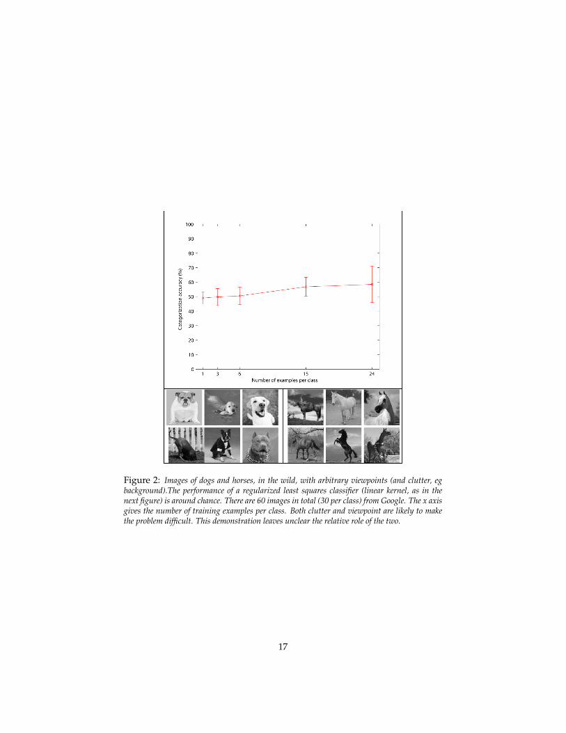
Figure 2: Images of dogs and horses, in the wild, with arbitrary viewpoints (and clutter, egbackground).The performance of a regularized least squares classifier (linear kernel, as in thenext figure) is around chance. There are 60 images in total (30 per class) from Google. The x axisgives the number of training examples per class. Both clutter and viewpoint are likely to makethe problem difficult. This demonstration leaves unclear the relative role of the two.
17
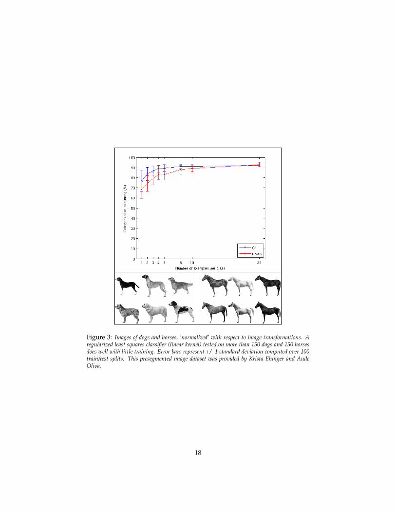
Figure 3: Images of dogs and horses, ’normalized’ with respect to image transformations. Aregularized least squares classifier (linear kernel) tested on more than 150 dogs and 150 horsesdoes well with little training. Error bars represent +/- 1 standard deviation computed over 100train/test splits. This presegmented image dataset was provided by Krista Ehinger and AudeOliva.
18
ized” images with respect to viewpoint, illumination, position and scale – theproblem of categorizing horses vs dogs is very easy: it can be done accuratelywith few training examples – ideally from a single training image of a dogand a single training image of a horse – by a simple classifier. In other words,the sample complexity of this problem is – empirically – very low. The taskin the figure is to correctly categorize dogs vs horses with a very small num-ber of training examples (eg small sample complexity). All the 300 dogs andhorses are images obtained by setting roughly the same viewing parameters– distance, pose, position. With these “rectified” images, there is no signifi-cant difference between running the classifier directly on the pixel representa-tion versus using a more powerful set of features (the C1 layer of the HMAXmodel).
3.1.2 Intraclass and viewpoint complexity
Additional motivation is provided by the following back-of-the-envelope esti-mates. Let us try to estimate whether the cardinality of the universe of possibleimages generated by an object originates more from intraclass variability – egdifferent types of dogs – or more from the range of possible viewpoints – in-cluding scale, position and rotation in 3D. Assuming a granularity of a fewminutes of arc in terms of resolution and a visual field of say 10 degrees, onewould get 103 − 105 different images of the same object from x, y translations,another factor of 103−105 from rotations in depth, a factor of 10−102 from rota-tions in the image plane and another factor of 10− 102 from scaling. This giveson the order of 108 − 1014 distinguishable images for a single object. On theother hand, how many different distinguishable (for humans) types of dogsexist within the “dog” category? It is unlikely that there are more than, say,102 − 103. From this point of view, it is a much greater win to be able to factorout the geometric transformations than the intracategory differences.
Thus we conjecture that the key problem that determined the evolution ofthe ventral stream was recognizing objects – that is identifying and categoriz-ing – from a single training image, invariant to geometric transformations. Incomputer vision, it has been known for a long time that this problem can besolved if the correspondence of enough points between stored models and anew image can be computed. As one of the simplest results, it turns out thatunder the assumption of correspondence, two training images are enough fororthographic projection (see [74]). Recent techniques for normalizing for affinetransformations are now well developed (see [80] for a review). Various at-tempts at learning transformations have been reported over the years (see forexample [57, 30] and for additional references the paper by Hinton [20]).
Our goal here is instead to explore approaches to the problem that do notrely on explicit correspondence operations and provide a plausible biologicaltheory for the ventral stream. Our conjecture is that the main computational goalof the ventral stream is to learn to factor out image transformations. We show hereseveral interesting consequences follow from this conjecture such as the hier-archical architecture of the ventral stream. Notice that discrimination without
19
any invariance can be done very well by a classifier which reads the pattern ofactivity in simple cells in V1 – or, for that matter, the pattern of activity of theretinal cones.
Open Problem It seems obvious that learning/using an input representationwhich is invariant to natural transformations (eg contained in the distribution) shouldreduce the sample complexity of supervised learning. It is less obvious what is the bestformalization and proof of the conjecture.
3.2 Templates and signatures
Summary. In this section we justify another assumption in the theory: a primitivecomputation performed by neurons is a dot product. This operation can be used bycortex to compute a signature for any image as a set of dot products of the image with anumber of templates stored in memory. It can be regarded as a vector of similarities to afixed set of templates. Signatures are stored in memory: recognition requires matchinga signature with an item in memory.
The theory we develop in Part I is informed by the assumption that a basicneural operation carried by a neuron can be described by the dot product be-tween an input vectors and a vector of synaptic weights on a dendritic tree.Part II will depend from the additional assumption that the vector of synapticweights can be stored and modified by an online process of Hebb-like learning.These two hypothesis are broadly accepted.
In this paper we have in mind layered architectures of the general typeshown in Figure 5. The computational architecture is memory-based in thesense that it stores during development sensory inputs and does very little interms of additional computations: it computes normalized dot products andpooling (also called aggregation) functions. The results of this section are inde-pendent of the specifics of the hierarchical architecture and of explicit refer-ences to the visual cortex. They deal with the computational problem of in-variant recognition from one training image in a layered, memory-based archi-tecture.
The basic idea is the following. Consider a single aperture. Assume a mech-anism that stores “frames”, seen through the aperture, as an initial pattern “outin the world” transforms from t = 1 to t = N under the action of a spe-cific transformation (such as rotation). For simplicity assume that the set oftransformations is a group. This is the “developmental” phase of learning thetemplates. At run time an image patch is seen through the aperture, and a setof normalized dot products with each of the stored templates (eg all transfor-mations of each template) is computed. A vector called “signature” is thenproduced by an aggregation function – typically a group average over non-linear functions of the dot product with each template. Suppose now that atsome later time (after development is concluded) the same image is shown,transformed in some way. The claim is that if the templates are closed underthe same group of transformations then the signature remains the same. Sev-eral aggregation functions, such as the average or even the max (on the group),acting on the signature, will then be invariant to the learned transformation.
20
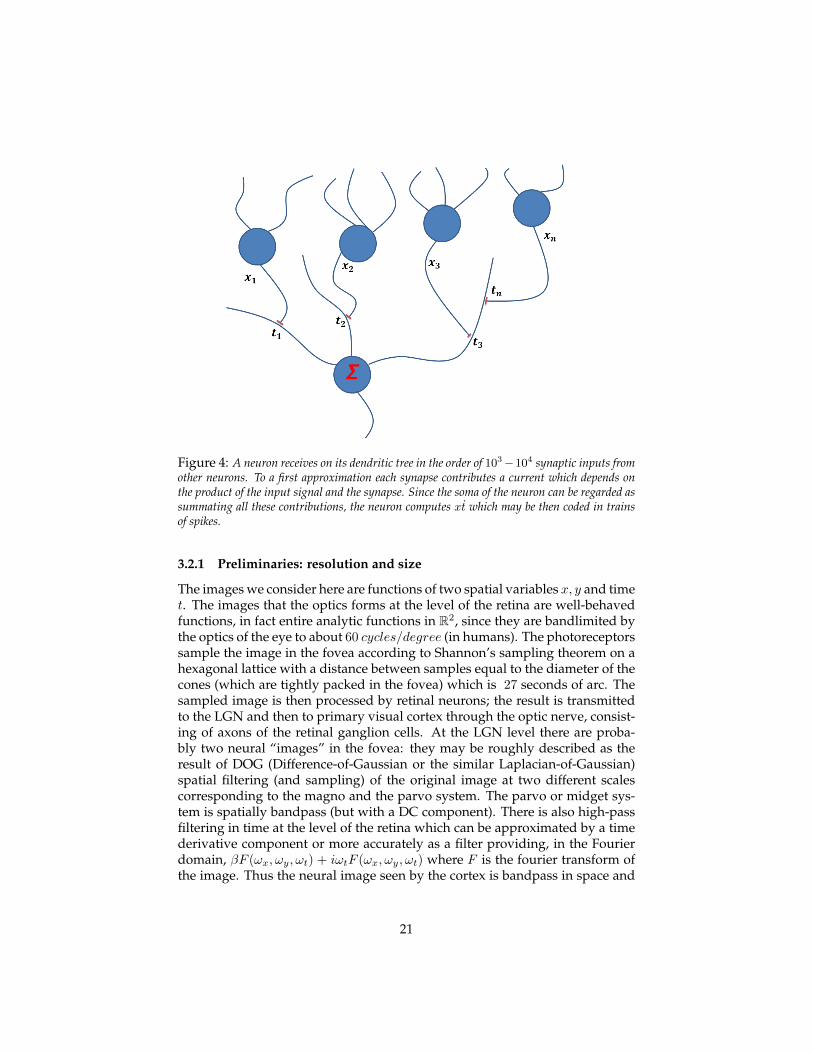
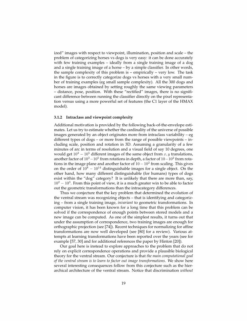
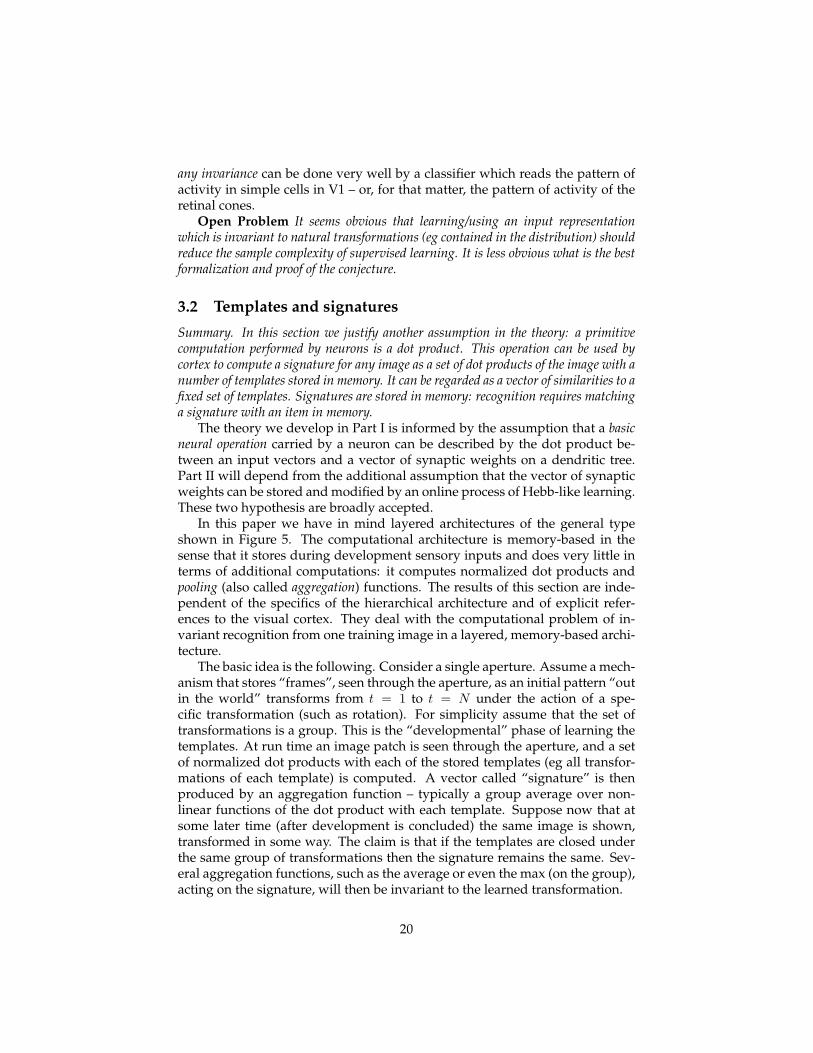
Figure 4: A neuron receives on its dendritic tree in the order of 103−104 synaptic inputs fromother neurons. To a first approximation each synapse contributes a current which depends onthe product of the input signal and the synapse. Since the soma of the neuron can be regarded assummating all these contributions, the neuron computes xt which may be then coded in trainsof spikes.
3.2.1 Preliminaries: resolution and size
The images we consider here are functions of two spatial variables x, y and timet. The images that the optics forms at the level of the retina are well-behavedfunctions, in fact entire analytic functions in R2, since they are bandlimited bythe optics of the eye to about 60 cycles/degree (in humans). The photoreceptorssample the image in the fovea according to Shannon’s sampling theorem on ahexagonal lattice with a distance between samples equal to the diameter of thecones (which are tightly packed in the fovea) which is 27 seconds of arc. Thesampled image is then processed by retinal neurons; the result is transmittedto the LGN and then to primary visual cortex through the optic nerve, consist-ing of axons of the retinal ganglion cells. At the LGN level there are proba-bly two neural “images” in the fovea: they may be roughly described as theresult of DOG (Difference-of-Gaussian or the similar Laplacian-of-Gaussian)spatial filtering (and sampling) of the original image at two different scalescorresponding to the magno and the parvo system. The parvo or midget sys-tem is spatially bandpass (but with a DC component). There is also high-passfiltering in time at the level of the retina which can be approximated by a timederivative component or more accurately as a filter providing, in the Fourierdomain, βF (ωx, ωy, ωt) + iωtF (ωx, ωy, ωt) where F is the fourier transform ofthe image. Thus the neural image seen by the cortex is bandpass in space and
21

Figure 5: Hierarchical feedforward model of the ventral stream – a modern interpretation of theHubel and Wiesel proposal (see [58]). The theoretical framework proposed in this paper providesfoundations for this model and how the synaptic weights may be learned during development(and with adult plasticity). It also suggests extensions of the model such as class specific modulesat the top.
22
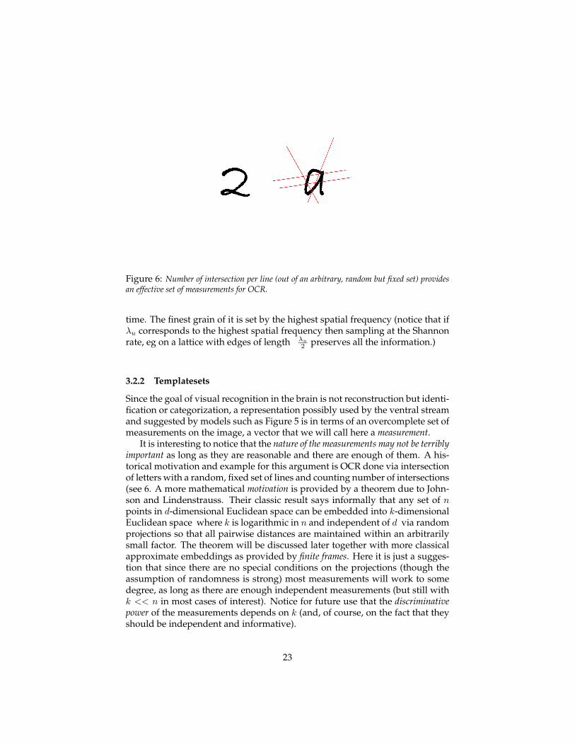
Figure 6: Number of intersection per line (out of an arbitrary, random but fixed set) providesan effective set of measurements for OCR.
time. The finest grain of it is set by the highest spatial frequency (notice that ifλu corresponds to the highest spatial frequency then sampling at the Shannonrate, eg on a lattice with edges of length λu
2 preserves all the information.)
3.2.2 Templatesets
Since the goal of visual recognition in the brain is not reconstruction but identi-fication or categorization, a representation possibly used by the ventral streamand suggested by models such as Figure 5 is in terms of an overcomplete set ofmeasurements on the image, a vector that we will call here a measurement.
It is interesting to notice that the nature of the measurements may not be terriblyimportant as long as they are reasonable and there are enough of them. A his-torical motivation and example for this argument is OCR done via intersectionof letters with a random, fixed set of lines and counting number of intersections(see 6. A more mathematical motivation is provided by a theorem due to John-son and Lindenstrauss. Their classic result says informally that any set of npoints in d-dimensional Euclidean space can be embedded into k-dimensionalEuclidean space where k is logarithmic in n and independent of d via randomprojections so that all pairwise distances are maintained within an arbitrarilysmall factor. The theorem will be discussed later together with more classicalapproximate embeddings as provided by finite frames. Here it is just a sugges-tion that since there are no special conditions on the projections (though theassumption of randomness is strong) most measurements will work to somedegree, as long as there are enough independent measurements (but still withk << n in most cases of interest). Notice for future use that the discriminativepower of the measurements depends on k (and, of course, on the fact that theyshould be independent and informative).
23
In summary we assume
• The ventral stream computes a representation of images that supports thetask of recognition (identification and categorization). It does not need tosupport image reconstruction.
• The ventral stream provides a signature which is invariant to geometrictransformations of the image and to deformations that are locally approx-imated by affine transformations
• Images (of objects) can be represented by a set of functionals of the image,eg measurements. Neuroscience suggests that a natural way for a neuronto compute a simple image measurements is a (possibly normalized) dotproduct between the image and a vector of synaptic weights correspond-ing to the tuning of the neuron.
Before showing how to built and invariant signature let us give a few defini-tions:
Definition 1. Space of images: X ⊆ L2(R2) ( or Rd) where
L2(R2) = I : R2 → R, s.t.∫| I(x, y) |2 dxdy <∞
〈I, t〉 =∫I(x, y)t(x, y)dxdy
Definition 2. Template set: T ⊆ X , (or Rd): a set of images (or, more generally,image patches)
Given a finite template set (|T | = T < ∞) we define a set of linear func-tionals of the image I :
〈I, ti〉, i = 1, ..., T.
Definition 3. The image I can be represented in terms of its measurement vectordefined with respect to the templateset T :
∆I = (〈I, t1〉, 〈I, t2〉, ..., 〈I, tT 〉)T
We consider here two examples for choosing a set of templates. Both ex-amples are relevant for the rest of the paper. Consider as an example the setof images in X ∈ Rd. The obvious choice for the set of templates is to be anorthonormal basis in the space of “images patches”, eg in Rd. Our first exam-ple is a variation of this case: the templateset T is assumed to be a frame (seeAppendix 23.1) for the n-dimensional space X spanned by n chosen images inRd, that is the following holds
24

A||I||2 ≤T∑k=1
| < I, tk > |2 ≤ B||I||2 (1)
where I ∈ Rd and A ≤ B. We can later assume that A = 1 − ε and B = 1 + εwhere ε can be controlled by the cardinality T of the templateset T . In thisexample consider for instance n ≤ T < d.
This means that we can represent n images by projecting them from I ∈ Rdto RT by using templates. This map F : Rd → RT is such that for all u, v ∈ X(where X is a n-dimensional subspace of Rd)
A ‖ u− v ‖≤‖ Fu− Fv ‖≤ B ‖ u− v ‖ .If A = 1 − ε and B ≤ 1 + ε where ε = ε(T ) the projections of u and v in RTmaintains the distance within a factor ε: the map is a quasi-isometry and canbe used for tasks such as classification. The second example is based on thechoice of random templates and a result due to Johnson and Lindenstrauss (J-L).
Proposition 1. For any set V of n points in Rd, there exists a map P : Rd → RTsuch that for all u, v ∈ V
(1− ε) ‖ u− v ‖≤‖ Pu− Pv ‖≤ (1 + ε) ‖ u− v ‖
where the map P is a random projection on RT and
kC(ε) ≥ ln(n), C(ε) =12(ε2
2− ε3
3).
The JL theorem suggests that good representations for classification anddiscrimination of n images can be given by T dot products with random tem-plates since they provide a quasi-isometric embedding of images.
Remarks
• The dimensionality of the measurement vector suggested by JL dependson n but not on d;
• The dimensions of the measurement vector are logarithmic in n;
• The fact that random templates are sufficient suggests that the precisechoice of the templates is not important, contrary to the present folk wis-dom of the computer vision community.
25

3.2.3 Transformations and templatebooks
The question now is how to compute a measurement vector that is capable notonly of discriminating different images but is also invariant to certain transfor-mations of the images. We consider geometric transformations of images dueto changes in viewpoints.We define as geometric transformations of the image I the action of the operatorU(T ) : L2(R2)→ L2(R2) transformations such that:
[U(T )I](x, y) = I(T−1(x, y)) = I(x′, y′), I ∈ L2(R2)
where T : R2 → R2 is a coordinate change.In general U(T ) : R2 → R2 isn’t a unitary operator. However it can be madeunitary defining
[U(T )I](x, y) = |JT |− 12 I(T−1(x, y))
where |JT | is the determinant of the Jacobian of the transformation. Unitarityof the operator will be useful later, (e.g. in 3.4.2).A key example of T is the affine case, eg
x′ = Ax + tx
where A ∈ GL(2,R) the linear group in dimension two and tx ∈ R2.
In fact, in most of this paper we will consider transformations that corre-spond to the affine group Aff(2,R) which is an extension of GL(2,R) (thegeneral linear group in R2) by the group of translations in R2. Let us nowdefine a key object of the paper:
Definition 4. Suppose now we have a finite set of templates that are closed under theaction of a group of transformations:
G = (g1, ..., g|G|), T = (t1, ..., tT ), |G|, T <∞
We assume that the basic element of our architecture, the memory based module, stores(during development) sequences of transformed templates for each template in the tem-plateset. We define the Templatebook as
Tt1,...,tT =
g0t1, g0t2, ..., g0tT
...g|G|t1, g|G|t2, ..., g|G|tT
.
the collection of all transformed templates. Each row corresponds to the orbit of thetemplate under the transformations of G.
26

3.3 Invariance and discrimination
Summary. If a signature is a dot product between the image and a template, then theaverage of any function of the dot product between all the transformations of the imageand the template is an invariant. Under some assumption this is equivalent to theaverage of any function of the dot product of the image and all the transformationsof the template. Thus an invariant can be obtained from a single image. However,invariance is not enough: discrimination is also important. Thus we go back to groundzero: we consider not only the average of a function of the dot product but the full orbit– corresponding to the set of dot products. For compact groups if two orbits have apoint in common then they are the same orbit. A distribution can be associated to eachorbit and a distribution can be characterized in terms of its moments which are groupaverages of powers of the dot products. The overall logic is simple with some problemsin the details. We also take somewhat of a detour in discussing sets of templates suchas frames, random projections etc.
We start with a rather idealized situation (group is compact, the image doesnot contain clutter) for simplicity. We will make our framework more realisticin section 3.4.
3.3.1 The invariance lemma
Consider the dot products of all transformation of an image with one compo-nent of the templateset t
∆G,I = (〈g0I, t〉, 〈g1I, t〉..., 〈g|G|I, t〉)T
Clearly,
∆G,I = (〈g0I, t〉, 〈g1I, t〉, ..., 〈g|G|I, t〉)T = (〈I, g−10 t〉, 〈I, g−1
1 t〉, ..., 〈I, g−1|G|t〉)T
where g−1 is the inverse transformation of g and ∆G,I is the measurement vec-tor of the image w.r.t the transformations of one template, that is the orbit ob-tained by the action of the group on the dot product. Note that the followingis mathematically trivial but important from the point of view of object recog-nition. To get measurements of an image and all its transformations it is notnecessary to “see” all the transformed images: a single image is sufficient pro-vided a templatebook is available. In our case we need for any image, just onerow of a templatebook, that is all the transformations of one template:
Tt = (g0t, g1t, ..., g|G|t)T .
Note that the orbits ∆I,G and ∆gI,G are the same set of measurements apartfrom ordering). The following invariance lemma follows.
Proposition 2. Invariance lemma Given ∆I,G for each component of the template-set an invariant signature Σ can be computed as the group average of a nonlinear
27
function, η, of the measurements which are the dot products of the image with alltransformations of one of the templates, for each template:
Σt[I] =1|G|
∑g∈G
η(〈I, gt〉). (2)
A classical example of invariant is η(·) ≡ | · |2, the energy
Σti(I) =1|G|
|G|∑j=1
|〈I, gjti〉|2
Other examples of invariant group functionals are
• Max: Σti(I) = maxj〈I, gjti〉
• Average: Σti(I) = 1|G|∑|G|j=1〈I, gjti〉
These functions are called pooling or aggregation functions. The original HMAXmodel uses a max of I gjti over j or the average of I gjti over j or the av-erage of (I gjti)2 over j. Often a sigmoidal function is used to describe thethreshold operation of a neuron underlying spike generation. Such aggrega-tion operations can be approximated by the generalized polynomial
y =
n∑i=1
wi xip
k +
(n∑i=1
xiq
)r (3)
for appropriate values of the parameters (see [29]). Notice that defining the p-norm of xwith ||x||p = (
∑ |xi|p) 1p , it follows thatmax(x) = ||x||∞ and energy−
operation(x) = ||x||2. Therefore the invariant signature,
Σ(I) = (Σt1(I),Σt2(I), ...,ΣtT (I))T
is a vector which is invariant under the transformations gj .
Remarks
• Group characters As we will see later using templates that are the charac-ters of the group is equivalent to performing the Fourier transform de-fined by the group. Since the Fourier transform is an isometry for alllocally compact abelian groups, it turns out that the modulo or modulosquare of the transform is an invariant.
28

• Pooling functions It is to be expected that different aggregation functions,all invariant, have different discriminability and noise robustness. Forinstance, the arithmetic average will support signatures that are invariantbut are also quite similar to each other. On the other hand the max, alsoinvariant, may be better at keeping signatures distinct from each other.This was the original reason for [58] to choose the max over the average.
• Signature Notice that not all individual components of the signature (avector) have to be discriminative wrt a given image – whereas all haveto be invariant. In particular, a number of poorly responding templatescould be together quite discriminative.
• Group averages Image blur corresponds to local average of pixel values. Itis thus a (local) group average providing the first image moment.
3.3.2 Discrimination and invariance: distance between orbits
An invariant signature based on the arithmetic average is invariant but likely tobe not discriminative enough. Invariance is not enough: discrimination must alsobe maintained. A signature can be however made more discriminative by usingadditional nonlinear functions of the same dot products. Next we discuss howgroup averages of a set of functions can characterize the whole orbit.
To do this, we go back to orbits as defined in equation 3.3.1. Recall that iff agroup is compact then the quotient group is a metric space. This implies that adistance between orbits can be defined (see Proposition 3). As we mentioned,if two orbits intersect in one point they are identical everywhere. Thus equalityof two orbits implies that at least one point eg image is in common.
The goal of this section is to provide a criterion that could be used in a bio-logically plausible implementation of when two empirical orbits are the sameirrespectively of the ordering of their points. Ideally we would like to give meaningto a statement of the following type: if a set of invariants for u is ε close to theinvariants associated with v, then corresponding points of the two orbits are εclose.
The obvious approach in the finite case is to rank all the points of the u setand do the same for the v set. Then a comparison should be easy (computa-tionally). Another natural approach is to compare the distribution of numbersassociated with the u set with the distribution associated with the v set. This isbased on the following axiom (that we may take as a definition of equivalencebetween the orbits generated by G on the points u and v,
Definition 5.p(u) = p(v) ⇐⇒ u ∼ v
where p is the probability distribution.
29
Thus the question focuses on how can probability distribution be com-pared. There are several metrics that can be used to compare probability dis-tributions such as the Kolmogoroff-Smirnoff criterion and the Wasserstein dis-tance. The K-S criterion is the simpler of the two. The empirical distributionfunction is defined as
Fn(u) =1n
∑IUi≤u
for n iid observations Ui, where I is the indicator function. The KolmogoroffSmirnoff statistic for a given other cumulative empirical distribution functionGn(u) is
Dn = supu|Fn(u)−Gn(u)|,where supu is the supremum of the set of distances. By the GlivenkoCantellitheorem, if the samples come from the same distribution, then Dn convergesto 0 almost surely.
An approach which seems possibly relevant, though indirectly, for neuro-science is related to the characterization of distributions in terms of moments.In fact, a sufficient (possibly infinite) number of moments uniquely character-izes a probability distribution. Consider an invariant vector m1(v) in Rd withcomponents m1
i , i = 1, · · · , d with (mi)1(v) = 1|G|∑j((v
j)i)1 where vj = gjv
and (vj)i is its i-component. Other similar invariant “moment” vectors suchas mp
i (v) = 1|G|∑j((v
j)i)p can be defined. Observe that intuitively a sufficientnumber ( p = 1, · · · , P ) of moments mp
i (v) determines uniquely (vj)i for all jand of course viceversa.
This is related to the uniqueness of the distribution which is the solution of themoment problem ensured by certain sufficient conditions such as the Carlemancondition
∑∞p=1
1
(m2p)12p
on the divergence of infinite sums of functions of the
moments mp. The moment problem arises as the result of trying to invert themapping that takes a measure to the sequences of moments
mp =∫xpdµ(x).
In the classical setting, µ is a measure on the real line. In this form the ques-tion appears in probability theory, asking whether there is a probability mea-sure having specified mean, variance and so on, and whether it is unique. Inthe Hausdorff moment problem for a bounded interval, which without loss ofgenerality may be taken as [0, 1], the uniqueness of µ follows from the Weier-strass approximation theorem, which states that polynomials are dense underthe uniform norm in the space of continuous functions on [0, 1]. In our case themeasure µ is a Haar measure induced by the transformation group.
The following lemma follows:
Lemma 1. p(u) = p(v) ⇐⇒ mpi (u) = mp
i (v),∀i, pThe lemma together with the axiom implies
30

Proposition 3. If ming||gu − v||2 = 0 then mpi (v) = mp
i (u) for all p. Conversely,if mp
i (v) = mpi (u) for i = 1, · · · , d and for all p, then the set of gu for all g ∈ G
coincides with the set of all gv for all g ∈ G.
We conjecture that a more interesting version of the proposition above shouldhold in terms of error bounds of the form:
Proposition 4. For a given error bound ε it is possible (under weak conditions to bespelled out) to chose δ and K such that if |mp
i (v)−mpi (u)| ≤ δ for p = 1, · · · ,K then
ming||gu− v||2 ≤ ε.This would imply that moments computed in Rk can distinguish in an in-
variant way whether v and u are equivalent or not, in other words whethertheir orbits coincide or not. We now have to connect Rk to Rd. The key obser-vation of course is that
〈I, g−1i t〉 = 〈giI, t〉
thus measurements of one of the images with ”shifts” of the template are equiv-alent to measurements of (inverse) shifts of the image with a fixed template.
3.3.3 Frames and invariants
We know that with a sufficient number of templates it is possible to control εand thus maintain distances among the points v and u and all of their |G| trans-lates (which do not need to be explicitly given: it is enough to have translatesof the templates in order to have all the dot products between each randomtemplate and all the translates of each point, eg image). Thus the overall pic-ture is that there is an embedding of n points and their translates in Rd into Rkthat preserves approximate distances.
Consider nowRk and the projections inRk of v and u and of their translates,that is P (v) = v and P (u) = u and P (vj) = vj etc. The same results wrtmoments above also hold in Rk. In other words, from a sufficient number ofmoments for each of the k coordinates, it is possible to estimate whether theorbits of u and v are the same or not. In particular, we conjecture that thefollowing result should hold
Proposition 5. For any given ε it is possible to chose δ and K such that if |mpi (v)−
mpi (u)| ≤ δ for p = 1, · · · ,K for all i = 1, · · · , k then ming||gu− v||2 ≤ ε.
The resulting diagram is in Figure 7: images are on the left, the action ofthe group generates from each image a series of transformed images that forman orbit of the group. The real action is on the right side (in Rk) where from asingle image u on the left the orbit associated to the group is generated by thedot products of u with each template and the associate orbit. The orbits of uand v can be discriminated by the moments of each coordinate of the imagesproviding two vectors of moments that discriminate between the two orbits butare invariant to the ordering of the transformed images. The diagram provides
31
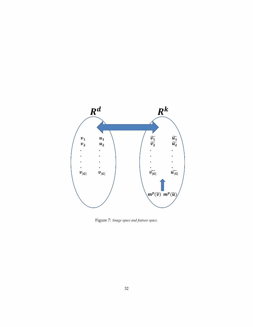
Figure 7: Image space and feature space.
32
an approach towards the characterization of the tradeoff between invarianceand discriminability.
3.3.4 Random projections and invariants: an extension of J-L
Let us first consider how the JL result could be extended to the situation inwhich n points in Rd are projected in Rk using k random templates and their|G| transformations induced by a group with |G| elements.
Proposition 6. For any set V of n points in Rd and for a group G of |G| elementsthere exists k random templates and for each of the template and its |G| transformssuch that for all u, v ∈ V
(1− ε) ‖ u− v ‖≤‖ P ′u− P ′v ‖≤ (1 + ε) ‖ u− v ‖
where the map P ′ includes the |G| transforms of each of k random projection on Rkand
kC(ε) ≥ ln(n) + ln(|G|), C(ε) =12(ε2
2− ε3
3)
The key point for biology is that the n vectors v and their |G| transforma-tions can be discriminated by random projections without the need to storeexplicitly the transformations of each vector: a single image of an object is suffi-cient for invariant recognition of other views of the object!
The previous result implies that by increasing the number of templates fromln(n) to ln(n)+ ln(|G|) it is possible to maintain distances among the original npoints and all of their |G| translates (which do not need to be explicitly given:it is enough to have translates of the templates in order to have all the dotproducts between each random template and all the translates of each point,eg image). Thus the overall picture is that there is an embedding of n pointsand their translates in Rd into Rk that preserves approximate distances. Theprevious result guarantees that the n images and all of their transforms canbe discriminated through their projections. The selectivity-invariance tradeoff isclear here: for a fixed number of templates (k) and a fixed accuracy (ε), there isan equivalent role for the number of discriminable objects, ln(n) and numberof transformations, ln(|G|), and a direct tradeoff among them.The key point for biology is that the n vectors v and their |G| transformationscan be discriminated by random projections without the need to store explic-itly the transformations of each vector.This observation allows to take measurements on the result of random projec-tions to obtain signatures that are either selective to identity and invariant totransformations or selective to the transformation and invariant to identity.
The question is how – in addition to (non-invariant) distances in Rn – wemay define invariants associated with each pattern which are the same for
33
every member of the set generated by the group. Notice that the Johnson-Lindenstrauss result implies that if u and v are very close (that is ||u− v|| ≤ η),their projections P (u) and P (v) are very close in every norm, in particularcomponent-wise (that is maxk|P (u)k − P (v)k| ≤ η).
Consider nowRk and the projections inRk of v and u and of their translates,that is P (v) = v and P (u) = u and P (vj) = vj etc. The same results wrtmoments above also hold in Rk. In other words, from a sufficient numberof moments for each of the k coordinates, it is possible to estimate whetherthe orbits of u and v are the same or not. We can the use the extension inproposition 6 of the JL theorem to connect Rd to Rk. In particular, a similarresult should hold to frame proposition above:
Proposition 7. For any given ε it is possible to chose δ and K such that if |mpi (v)−
mpi (u)| ≤ δ for p = 1, · · · ,K for all i = 1, · · · , k then ming||gu− v||2 ≤ ε.
The diagram of Figure 7 should then describe the situation also for randomprojections.
Both random projections and frames behave like a quasi-isometry satisfy-ing a frame-type bound. Of course random projections are similar to choos-ing random images as templates which are not natural images! Part II how-ever considers templates which are Gabor wavelets (they emerge as the topeigenfunctions of templatebooks learned from “randomly” observed imagesundergoing an affine transformation). These templates are likely to be bettercharacterized as randomly sampled frames than as random vectors! The mostrelevant situation is therefore when the templates are derived from a randomsubsampling from an overcomplete set. Corollary 5.56 of Vershynin “Introduc-tion to non-asymptotic analysis of random matrices”) gives conditions underwhich a random subset of size N = O(nlogn) of a tight frame in Rn is an ap-proximate tight frame ([76]).
Theorem 1. Consider a tight frame ui, i = 1, ...,M in Rn with frame boundsA = B = M . Let number m be such that all frame elements satisfy ||ui||2 ≤
√m.
Let vi, i = 1, ..., N be a set of vectors obtained by sampling N random elementsfrom the frame ui uniformly and independently. Let ε ∈ (0, 1) and t ≥ 1. Then thefollowing holds with probability at least 12n−t
2: if N ≥ C( tε )
2mlogn then vi is aframe in Rn with bounds A = (1 − ε)N and B = (1 + ε)N . Here C is an absoluteconstant. In particular, if this event holds, then every x ∈ Rn admits an approximaterepresentation using only the sampled frame elements.
3.3.5 Compact groups, probabilities and discrimination
In particular if G is a compact group, called G, dg is a finite measure so thatgI can be seen as a realization of a random variable with values in the signalspace. A signature can be defined associating a probability distribution to eachsignal. Such a signature can be shown to be invariant and discriminant.
34

More precisely, if G is a compact group there is a natural Haar probability mea-sure dg.For any I ∈ X , the space of signals, define the random variable,
ZI : G → X , ZI(g) = gI.
Denote by PI , the law (distribution) of ZI , so that PI(A) = dg(Z−1I (A)) for any
borel set A ⊂ X .Let
ΦP : X → P(X ), ΦP (I) = PI ,
where P(X ) is the space of probability distribution on XWe have the following fact.
Fact 1. The signature ΦP is invariant and discriminant i.e. I ∼ I ′ ⇔ PI = PI′ .
Proof. We first prove that I ∼ I ′ ⇒ PI = PI′ .By definition PI = PI′ iff ∀ A ⊆ X∫
A
dPI(s) =∫A
dPI′(s)
This expression can be written equivalently as:∫Z−1I (A)
dg =∫Z−1I′ (A)
dg
where
Z−1I = g ∈ G s.t. gI ∈ A
Z−1I′ = g ∈ G s.t. gI ′ ∈ A = g ∈ G s.t. ggI ∈ A
Now note that ∀ A ∈ X if gI ∈ A ⇒ gg−1gI = gg−1I ′ ∈ A, i.e. g ∈ Z−1I (A) ⇒
gg−1 ∈ Z−1I′ (A). The inverse follows noticing that g ∈ Z−1
I′ (A) ⇒ gg ∈Z−1I (A). Therefore Z−1
I (A) = Z−1I′ (A)g, ∀A. Using this observation we have:∫
Z−1I (A)
dg =∫
(Z−1I′ (A))g
dg =∫Z−1I′ (A)
dg
where in the last integral we used the change of variables on g = gg−1 and theinvariance property of the haar measure; this proves the implication.
To prove the implication PI = PI′ ⇒ I ∼ I ′ note that PI − PI′ = 0 is
equivalent to:∫Z−1I′ (A)
dg −∫Z−1I (A)
dg =∫Z−1I (A)4Z−1
I′ (A)
dg, ∀A ∈ X
35
where with4we mean the symmetric difference. This impliesZ−1I (A)4Z−1
I′ (A) =∅ or equivalently
Z−1I (A) = Z−1
I′ (A), ∀ A ∈ XIn other words of any element in A there exist g′, g′′ ∈ G such that g′I = g′′I ′.This implies I = g′−1
g′′I ′ = gI ′, g = g′−1g′′, i.e. I ∼ I ′.
The signature ΦP does not have a natural vector representation. One wayto achieve such a representation is to consider the relationship between proba-bility distribution and measurements.
3.3.6 Measurements and probability distributions
We begin by considering X to be a d dimensional space and T ⊂ X an or-thonormal basis (we will later relax this last assumption). Then we can de-fine (with some abuse of notation) T : X → Rd, T (I) = (〈I, ti〉)i, ti ∈ T ,‖T (I)‖d = ‖I‖, and the random variable
ZTI : G → Rd, ZTI (g) = T gI.Denote by P TI , the law (distribution) of ZTI , so that P TI (A) = dg((ZTI )−1(A))for any borel set A ⊂ Rd and let
ΦTP : X → G(Rd), Φ(I) = P TI ,
where P(X ) be the space of probability distribution on Rd
Fact 2. If T is an orthonormal basis ΦTP is discriminant and invariant.
Proof. The proof follows the one in Fact 1 after noticing that T : X → Rd is anisometry and therefore preserve the volumes which implies:
P TI (A) = dg(Z−1T I (A)) = dg(Z−1
I (A)) = PI(A), ∀A ∈ X .
Fact 3. If T is a frame ΦTP (or Johnson Lindenstrauss), ΦTP is discriminative andinvariant.
Proof. Suppose P TI (A) = P TI′ (A), ∀A ∈ X . Following the demonstration inFact 1 we have that this implies
T gI − T g′I ′ = 0, ∃ g′ ∈ (ZTI′ )−1(A), ∀ g ∈ (ZTI )−1(A), A ∈ X .
Therefore T (gI − g′I ′) = 0; Being T a frame it implies gI − g′I ′ = 0 ⇒ I ′ =gI, g = g′−1
g, i.e., I ∼ I ′.If I ∼ I ′ we have (following again the same reasoning done in Fact 1) that g ∈(ZTI )−1(A) ⇒ gg−1 ∈ (ZTI′ )
−1(A) and g ∈ (ZTI′ )−1(A) ⇒ gg ∈ (ZTI )−1(A).
Therefore (ZTI )−1(A) = (ZTI )−1(A)g and using the Haar measure invariancewe have proven the implication I ∼ I ′ ⇒ P TI = P TI′ .
36
3.3.7 Moments
As we mentioned earlier, the moment problem concerns the question whetheror not a probability distribution (or, equivalently, the associated random vari-able) is uniquely determined by the sequence of moments, all of which aresupposed to exist, finite. The following result due to Papoulis [Probability,Random variables and Stochastic Processes, pg. 72− 77, 1991] is useful:
Fact 4. Give two distribution P,Q ∈ P(X ), let
µn =∫
RdxnZ(I)dx, Z = P,Q x ∈ Rd
denote the n−th central moment. Then P = Q if and only if chP (t) = chQ(t) wherechZ(t) is the characteristic function of the distribution Z(x) built from its momentsµn:
chZ(t) = F[Z(x)](t) = 1 + itµ1 − 12!t2µ2 − 1
3!t3µ3 +
14!t4µ4 + ....
We can now define the map M : P(Rd)→ R×Nd and let
ΦM : X → P(Rd), ΦTM (x) = M(P Tx ).
where M maps the probability distribution P Tx into its moments (and cross-moments).
Fact 5. The signature ΦTM is invariant and discriminative, being T an orthonormalbasis, Johnson Lindenstrauss or a frame.
Proof. From above we have that the moments determine the characteristic func-tion which uniquely determines the probability distribution. We then followthe proofs in the previous paragraph.
3.4 Partially Observable Transformations (POTs)
Summary. The results described so far assume compactness of the transformationgroup and assume that all transformations are “visible”. This is not fully realistic(though of course there are grids of cells and motion could be discretized). In this sec-tion we show how to relax the assumptions, though some work still needs to be done.
The invariance lemma is a key property that depends in our proof on thetransformations having a compact group structure. As it turns out, it is pos-sible to derive some invariance property under more general conditions. Wedescribe here the following setup as one of the possible generalizations. Con-sider the case of translation of the image or image patch. Let us assume that thetranslation is on a torus (around the observer) but that only part of the torusis visible through a “window” interval, e.g an interval I ∈ [−A,+A]. Thus thetransformations correspond to a compact group which is only partially observ-able.
37

3.4.1 Orbits and fragments
Notice that the prototypical group in the biological case consists of an abeliansubgroup of the affine group. As a key case, consider translation which isabelian but only locally compact.
3.4.2 Invariance Lemma for POTs
Let G be a locally compact Abelian group and dg the associated Haar measure.Let T : G → B(X ), Tg = T (g) be a representation of G on X (see appendix 22).
Example 1. Let X = L2(R2), and (TgI)(x) = I(σ−1g (x)), where σg : R2 → R2,
with g ∈ G, is a representation of a group G. In particular we can consider G to bethe affine group so that σgr = Ar + b and σ−1
g r = A−1r − b, where b ∈ R2 andA : R2 → R2 is a unitary matrix. It is easy to see that in this case Tg is linear andT ∗g I(r) = I(σgr) for all g ∈ G and r ∈ R2. Moreover, T ∗g Tg = I so that g 7→ Tg is aunitary representation of G on X .
In the following we consider the continuous (and more general) version of eq.(2), the invariance lemma:
Invariance Lemma. Let m,h : X → R2 with m(I) =∫h(TgI)dg. Then m is
invariant:m(Tg′I) =
∫h(Tg′TgI)dg =
∫h(Tg′gI)dg = m(I), (4)
for all I ∈ X , g′ ∈ G.
Observation. Note that in the case the group of transformations is discreteand h(I) = η(〈I, t〉) for t, I ∈ X , η : R2 → R2 measurable, and T is a unitaryrepresentation, then
η(〈TgI, t〉) = η(⟨I, Tg−1t
⟩).
and eq. (4) is exactly (2) in the continuous case.
Invariance Lemma for POTs. Let G0 ⊂ G and m0, h : X → R2 with m0(I) =∫G0h(TgI)dg.
Clearly, in this case m0 is not invariant,
m0(I)−m0(Tg′I) =∫G0
h(TgI)dg −∫G0
h(Tg′TgI)dg 6= 0, g, g′ ∈ G (5)
The second integral of (5) can be written, with the variable change g = g′g as∫G0
h(Tg′Tg)I)dg =∫G0
h(Tg′gI)dg =∫g′−1G0
h(TgI)dg
38

where the last equality is true since we renormalize the operator Tg w.r.t. itsJacobian (see 3.2.3). With abuse of notation calling g = g:
m0(I)−m0(Tg′I) =∫G0
h(TgI)dg −∫g′−1G0
h(TgI)dg
=∫G0∆g′−1G0
h(TgI)dg.
where with ∆ we indicate the symmetric difference. If G0,I = g′ ∈ G | h(TgI) =0,∀g ∈ G0∆g′−1G0, then,
m0(I) = m0(Tg′I), ∀g′ ∈ G0,I .
Example 2. The interpretation of G0,I can be made clear considering X = L2(R) andh(I)(x) = |f(x)|2, I ∈ X . Let (TτI)(x) = I(x+τ), I ∈ X , τ ∈ R and G0 = [−π, π].In this case, g′−1G0 = [−π − τ, π − τ ].
3.5 Hierarchical architectures: global invariance and local sta-bility
Summary. In this section we find that the one-layer network, though globally invari-ant, cannot provide robust signatures for parts of the image. A hierarchical architectureof the same modules overcomes these limitations. The section shows that a hierarchicalarchitecture of layers of dot products and pooling operations can be at each layer stablefor small perturbations, locally invariant, covariant and, finally at the top, globallyinvariant
3.5.1 Limitations of one layer architectures: one global signature only
The architecture described so far is a one layer architecture – a 2D array ofmemory-based modules which, for each image, compute a single signaturewhich is invariant to a group of global, uniform transformations such as theaffine group. We conjecture that the architecture is optimal for (Gaussian) clut-ter since matched filters are optimal in the L2 sense and the module performsa normalized dot-product – effectively a correlation (a max aggregation func-tion would then compute the max of the correlation, an algorithm known asmatched filter). Evolution may have in fact discovered first the one layer archi-tecture: there is some evidence of correlation-based, non-invariant recognitionin insects such as bees. The one-layer architecture has, however, a few weak-nesses:
• Fragility to image perturbations such as non uniform warping or smallshifts of image parts
• Memory storage issues when many object classes have to be recognizedwith tolerance to local and global affine transformations
39

The first problem is due to the global nature of the implemented invariance. Inthe next paragraphs we are going to see how a hierarchical architecture maysolve this problem.
3.5.2 The basic idea
Consider a hierarchical architecture such as in Figure 8. We assume that eachof the nodes
∧is invariant for shifts of a pattern within its receptive field; we
also assume that the output layer at each level is covariant (see later). Assumethat the receptive field of each node overlaps by 1
2 the neighboring ones oneach side at each level of the architecture. Start from the highest level. Assumethat deformations are local translation of a patch. Consider now the followingexamples. First assume that there is a minimal distance between patches (Aand B in the figure) of 3 pixels. It is easy to see that each of A and B has adistinct signature at the first level in 2 different nodes. Each of A or B canshift by arbitrary amounts without changing their signature. So each one isan “object” at the first level in terms of their signatures, invariant to shifts.They compose a new object (AB) at the second level if their distance is between3 ≤ d ≤ 4 and so on for higher levels. This is a situation in which A and Bare each a part – like an eye and a mouth in a face, each part is invariant toshifts, the object AB is also invariant and is tolerant to “small” deformations(distance between A and B). There other cases. For instance, assume that thedistance between A and B is 1 ≤ d ≤ 3. Then for each shift there is always a∧
which “sees” A, another one which “sees” B and a third one which “sees”AB. In this case AB are parts of an object AB, all represented in an invariantway at the first level. However, the object AB is not tolerant to deformationsof the distance between A and B (this happens only if objects are representedat higher levels than parts in the hierarchy). Finally, if the distance between Aand B is less than 1 then AB is always an object at all levels. It is intriguing tospeculate that this kind of properties may be related to the minimal distancesinvolved in crowding?
3.5.3 A hierarchical architecture: one dimensional translation group
In the following we are going to focus, as an easy example, on the locally com-pact group of one dimensional translations implemented by the operator
Tξ : X → X , (TξI)(τ) = I(τ − ξ), I ∈ X , ξ ∈ R .We fix the following basic objects:
• X = L2(R), space of images.
• T ⊂ X , |T | <∞, the template set.
• η : X → X a non-linear function.
• Kn : R → 0, 1 the characteristic function of the interval Pn ⊆ R wherePn−1 ⊆ Pn, ∀ n = 1, ..., N or Gaussian functions of σn width.
40
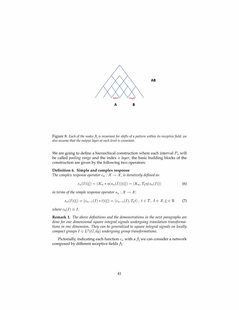
Figure 8: Each of the nodes∧
is invariant for shifts of a pattern within its receptive field; wealso assume that the output layer at each level is covariant.
We are going to define a hierarchical construction where each interval Pn willbe called pooling range and the index n layer; the basic building blocks of theconstruction are given by the following two operators:
Definition 6. Simple and complex responseThe complex response operator cn : X → X , is iteratively defined as:
cn(I)(ξ) = (Kn ∗ η(sn(I)))(ξ) = 〈Kn, Tξη(sn(I))〉 (6)
in terms of the simple response operator sn : X → X :
sn(I)(ξ) = (cn−1(I) ∗ t)(ξ) = 〈cn−1(I), Tξt〉 , t ∈ T , I ∈ X , ξ ∈ R (7)
where c0(I) ≡ I .
Remark 1. The above definitions and the demonstrations in the next paragraphs aredone for one dimensional square integral signals undergoing translation transforma-tions in one dimension. They can be generalized to square integral signals on locallycompact groups I ∈ L2(G, dg) undergoing group transformations.
Pictorially, indicating each function cn with a∧
we can consider a networkcomposed by different receptive fields
∧:
41

cn is the complex cell response at layer n and σn may be equal or larger thanσn−1.Notice that the patch of the image seen at layer n is at least as large as the patchseen at level n − 1, that is σneff ≥ σn−1
eff . In general σneff increases (rapidly)with n where with σeff we mean the image part effectively seen by a complexresponse at layer n.
3.5.4 Properties of simple and complex responses
We provide now our definition of covariance and invariance for the set of re-sponses cn at each layer n of the architecture. We, for simplicity are focusing ontranslations in 1D. However we can generalize the reasoning to translations inx, y which shifts “stuff” across receptive fields. In fact we can think of layers ateach level indexed by orientation and scale. Thus our invariance and covari-ance definitions are for a given orientation and scale.For 1D translations we are interested into studying the following two proper-ties:
42
1. Covariance: the operator f : X → X is covariant with respect transla-tions if:
f(Tξ(I)) = Tξ(f(I)), ∀ I ∈ X , ξ ∈ R
2. r−invariance: the operator f : X → X is r−invariant for I ∈ X withrespect to translations if:
f(Tξ(I)) = f(I), ξ ∈ [0, r], r ∈ R
Remark 2. Notice that many non-linear functionals are so-called space- or time-invariant, e.g. NL-L systems, Volterra series, etc.. In this paper, we assume thatcortical layers in visual cortex can be modeled by linear convolutions, which are triv-ially covariant, followed by memoryless non-linearities, which maintain covariance.
Remark 3. In principle, the arguments of these sections apply also to scale and ro-tation under the assumption that the network is X-invariant (instead of simply shift-invariant). If the network treats scale or rotation in the same way as x, y (with con-volution and local pooling) the same arguments should apply. In practice, as we willshow, in the hierarchical architecture after the first layer all transformations can beapproximated as shifts within a 4-cube of wavelets (see later).
3.5.5 Property 1: covariance
The covariance of the complex response is a key ingredient in the analysis ofthe invariance; we prove:
Proposition 8. The operator cn is covariant with respect to translations.Let cn : X → X the complex response at layer n and I ∈ X then:
cn(TτI) = Tτ (cn(I)), ∀τ ∈ R .
Proof. We prove the proposition by induction. For n = 1 the covariance of thes1(I) function follows from:
s1(TτI)(τ) = 〈TτI, Tτ t〉 = 〈I, Tτ−τ t〉 = s1(I)(τ − τ) = (Tτs1(I))(τ)
The covariance of the c1(I) follows from:
c1(TτI)(τ) =∫K1(τ − τ)η(s1(TτI))(τ)dτ
=∫K1(τ − τ)η(s1(I))(τ − τ)dτ
=∫K1(τ − τ − τ)η(s1(I)(τ))dτ = c1(I)(τ − τ)
= (Tτ c1(I))(τ)
43

where on the second line we used the covariance property of s1(I) and on thethird we used the change of variable τ = τ − τ .Suppose now the statement is true for n; by definition:
sn+1(TτI)(τ) = 〈cn(TτI), Tτ t〉 = 〈Tτ cn(I), Tτ t〉 = 〈cn(I), Tτ−τ t〉= sn+1(I)(τ − τ) = (Tτsn+1(I))(τ)
Therefore
cn+1(TτI)(τ) =∫Kn+1(τ − τ)η(sn+1(TτI)(τ))dτ
=∫Kn+1(τ − τ)η(sn+1(I)(τ − τ))dτ
= cn+1(I)(τ − τ) = (Tτ cn+1(I))(τ)
where in the fourth line we used the change of variables τ − τ = τ .By induction, the statement is true for all layers.
3.5.6 Property 2: partial and global invariance
We now prove that the functions cn are approximately invariant (locally in-variant) to translations within the range of the pooling. We further prove thatthe invariance increases from layer to layer in the hierarchical architecture.Inthe following, for reasons that will be clear later we choose as non linearity themodulus function, η ≡ | · |.
Proposition 9. Let cn : X → X the complex response at layer n and I ∈ X then:
cn(TτI)(τ) = cn(I)(τ), I ∈ X , (8)
if|sn(I)(τ)| = 0 τ ∈ Pn∆TτPn
where ∆ is the symmetric difference.
Proof. Let the pooling at layer n be achieved by a characteristic function on theinterval Pn We have
cn(TτI)(τ)− cn(I)(τ) = cn(I)(τ − τ)− cn(I)(τ)
=∫
R
(Kn(τ − τ − τ)−Kn(τ − τ)
)|sn(I)(τ)|dτ
=∫Pn∆TτPn
|sn(I)(τ)|dτ
where on the first line we used the covariance properties of the function cn(I).
44

Further the invariance is increasing from layer to layer since the effective pool-ing range at layer n will be
P effn = Pn × Pn−1 × · · · × P0
Consequently for each transformation there will exists a layer such that thecomplex response is invariant to the transformation. We have
Theorem 2. Let I ∈ X , cn : X → X the complex response at layer n. Let ξ ∈[0, τ ], τ ∈ R, we have that cn is τ−invariant for sone n, i.e.
cn(TξI) = cn(I), ∃ n s.t. ∀m ≥ n, ξ ∈ [0, τ ]
Proof. The proof comes from the fact that for any ξ ∈ [0, τ ] there always existan n = n such that forallτ ∈ Pn∆TτPn, |sn(I)(τ)| = 0. The proof follows from9.
Remark 4. If in 9 instead of choosing the characteristic function of the interval Pn weuse a Gaussian function exp(−x2/2σn) a similar result is obtained:
cn(TτI)(τ) = cn(I)(τ) +O( τ2
2σ2n
), ∀τ ∈ [0, σn], τ ∈ R.
Remark 5. There are multiple scales (at each layer). We can think of them as differentresolution units corresponding to different sizes of complex cells – like multiple latticesof photoreceptors of different sizes and different separations. The size of the complexcells also increases from layer to layer and defines how large a part is at each layer– from small parts in the first layer to parts of parts in intermediate layers, to wholeobjects and images at the top. Notice that the term parts here really refers to patches ofthe image. Notice that our theory may provide a novel definition of Part as the setof patches which has an invariant signature – at some level of the architecture – underaffine transformations.
3.5.7 Property 3: stability to perturbations
In the paragraphs above we assumed, for simplicity, to have one template ateach layer. We will now suppose to have a set of templates at each layer thatform a frame with good frequency localization properties (e.g. wavelets)
Tn = tin, i = 1, ..., Tn
an ‖I‖2 ≤( Tn∑i=1
| ⟨tinn , I⟩ |2) 12
= ‖I‖`2 ≤ bn ‖I‖2 , an < bn ∈ R+ I ∈ X .
Let the non−linearity η : X → X be the modulus square function σ(·) = | · |.Using this formalism we can write the complex response cn(I) at layer n bycomponents using the multi−index λ ≡ (i0, ..., in−1) as follow.Let Cn : X → `2(RT ), T = T0 + ...+ Tn, the map
I −→ cλn(I) = cin−1,in−2,...,i1n (I) = Kn ∗ |tin−1
n−1 ∗Kn−1 ∗ |tin−2n−2 ∗ · · · ∗ |ti11 ∗ I| · · · |
I ∈ X , i1 = 1, ..., T1; ...; in−1 = 1, ..., Tn−1
45
with norm in `2(RT ),
‖cn(I)‖`2 =∑
in−1,in−2,...,i1
(|Kn ∗ |tin−1
n−1 ∗Kn−1 ∗ |tin−2n−2 ∗ · · · ∗ |ti11 ∗ I| · · · ||2
) 12
We study now, starting from the top cn(I) complex response, the toleranceof the hierarchical representation to small perturbations I → I + δI . As in theprevious paragraph, let Tn = tinn , i = 1, ..., Tn a frame at layer n.
Theorem 3. Let I ∈ X . We have
‖cn(I)− cn(I + δI)‖`2 ≤n∏i=1
bi ‖δI‖∞ (9)
with
‖cn(I)− cn(I + δI)‖`2 =( T1,...,Tn∑i1,...,in
|tinn ∗ [ci1,...,in−1n (I)− ci1,...,in−1
n (I + δI)|2) 1
2
(10)and
‖δI‖∞ = supτ |δI(τ)|The theorem says that the representation is continuous to perturbations from L2(R) to`2(RT
n
), T =∑ni=1 Ti
Proof. Being Tn = tinn , i = 1, ..., Tn a frame we have
‖cn(I)− cn(I + δI)‖2`2 =T1,...,Tn∑i1,...,in
|tinn ∗ [ci1,...,in−1n (I)− ci1,...,in−1
n (I + δI)]|2
≤ b2n
T1,...,Tn−1∑i1,...,in−1
|ci1,...,in−1n (I)− ci1,...,in−1
n (I + δI)|2.
Using the definitions of complex and simple response, cinn (I) = Kn ∗ |sinn (I)|and sinn (I) = t
in−1n−1 ∗ cn−1(I)
‖cn(I)− cn(I + δI)‖2`2 ≤ b2nT1,...,Tn−1∑i1,...,in−1
|Kn∗(|tin−1n−1 ∗ci1,...,in−2
n (I)|−|tin−1n−1 ∗ci1,...,in−2
n (I+δI)|)|2
The convolution with Kn is a lowpass filter applied to the modulus square i.e.is decreasing the energy content of the signal by filtering. Further using thecontraction properties of the modulus function i.e. ||a| − |b|| ≤ |a− b|
‖cn(I)− cn(I + δI)‖2`2 ≤ b2nT1,...,Tn−1∑i1,...,in−1
|tin−1n−1 ∗
(ci1,...,in−2n (I)−ci1,...,in−2
n (I+δI)|)|2
46
The last equation has the same form of eq. (10) with the frame factor b insteadof the sum over in. Repeating the reasoning for all layers
‖cn(I)− cn(DI)‖`2 ≤n∏i=2
b2i∑i1
|ti11 ∗ (I − (I + δI))|2 ≤n∏i=1
b2i ‖δI‖2∞
Taking the root square ends the proof.
3.5.8 A hierarchical architecture: summary
In the following we are going to extend the reasoning done in the previousparagraphs to a general transformation of a locally compact group G imple-mented by the operator
Tg : X/Y → Y, (TgI)(τ) = I(gτ), I ∈ X/Y, g ∈ G.where X and Y are defined below among other basic objects:
• X = L2(R2).
• Y = L2(G, dg), where dg is the group invariant Haar measure.
• T ⊂ X/Y , |T | <∞, the template set.
• η : Y → Y a non-linear function.
• Kn : Y → Y the characteristic function of the intervals P1 ⊆ ... ⊆ Pn,Pi ⊂ Y or Gaussians with σn width.
The definitions of simple and complex response are similar to those given forthe one dimensional translation group. However there is a major difference,although irrelevant for the covariance, invariance properties of the construc-tion: the first simple response is an operator that maps the image space X intoY ; higher order responses instead are operators defined from Y into itself.
Definition 7. Simple and complex responseThe complex response operator cn : Y → Y , is iteratively defined as:
cn(I)(ξ) = (Kn ∗ η(sn(I)))(ξ) = 〈Kn, Tgη(sn(I))〉 (11)
in terms of the simple response operator sn : X/Y → Y :
sn(I)(ξ) = (cn−1(I) ∗ t)(ξ) = 〈cn−1(I), Tξt〉 , t ∈ T , I ∈ X , g ∈ G (12)
where c0(I) ≡ I .
Same kind of results obtained before for covariance, invariance and robust-ness to local perturbations can be obtained.
47
3.6 A short mathematical summary of the argument.
The theory just described has a simple mathematical structure, despite themixed biological details. We summarize in this appendix.
3.6.1 Setting
Let (X , 〈·, ·〉) be a real separable Hilbert space, e.g. X = L2(R2). Let L(X ) bethe space of linear operators to and from X .
A measurement is defined as a functional m : X → R. A signature is a mapφ : X → `2 and can be viewed as a collection of measurements.
3.6.2 Linear measurements: bases, frames and Johnson Lindenstrauss lemma
Claim: Linear measurements give rise to isometric or quasi-isometric signa-tures.
Let T ⊂ X be countable and
s : X → `2, st(I) = 〈I, t〉 t ∈ T .
If T is an orthonormal basis I =∑t∈T st(I)t and ‖s(I)‖2 = ‖I‖where ‖s(I)‖22 =∑
t st(I)2.If T is a frame, by definition, A ‖I‖ ≤ ‖s(I)‖2 ≤ B ‖I‖, with 0 < A ≤ B <∞.Finally, if X is a set of n points in RN and T a suitable finite set of p, possi-bly random, vectors. by the Jonson and Lindenstrauss lemma (1 − ε) ‖I‖ ≤‖s(I)‖2 ≤ (1 + ε) ‖I‖, as soon as p ≥ 8 log n/ε2.
3.6.3 Invariant measurements via group integration
Claim: Invariant measurements can be obtained via local group integration.Let G be a locally compact Abelian group and dg the associated Haar mea-
sure. Let T : G → B(X ), Tg = T (g) be a representation of G on X .
Example 3. Let X = L2(R2), and (TgI)(I) = I(σ−1g (I)), where σg : R2 → R2,
with g ∈ G, is a representation of a group G. In particular we can consider G to bethe affine group so that σgr = Ar + b and σ−1
g r = A−1r − b, where b ∈ R2 andA : R2 → R2 is a unitary matrix. It is easy to see that in this case Tg is linear andT ∗g x(r) = x(σgr) for all g ∈ G and r ∈ R2. Moreover,redefining the representationdividing by the transformation Jacobian we have T ∗g Tg = I so that g 7→ Tg is a unitaryrepresentation of G on X .
3.6.4 Observation
If t, I ∈ X , and T is a unitary representation, then
〈TgI, t〉 =⟨I, T ∗g t
⟩=⟨I, T−1
g t⟩
=⟨I, Tg−1t
⟩.
48

For σ : R→ Rmeasurable, let
c : X → R, c(I) =∫σ(〈I, Tgt〉)dg,
then c is invariant.
3.6.5 Approximately invariant measurements via local group integration
Claim: Approximately invariant measurements can be obtained via local groupintegration.
Let m,h : X → Rwith m(I) =∫h(TgI)dg. Then m is invariant:
m(Tg′I) =∫h(Tg′TgI)dg =
∫h(Tg′gI)dg = m(I),
for all I ∈ X , g′ ∈ G.
Let G0 ⊂ G and m0, h : X → Rwith m0(I) =∫G0h(TgI)dg.
Clearly, in this case m0 is not invariant,
m0(I)−m0(Tg′I) =∫G0
h(TgI)dg −∫G0
h(Tg′gI)
=∫G0
h(TgI)dg −∫g′−1G0
h(TgI)dg =∫G0∆g′−1G0
h(TgI)dg.
If G0,I = g′ ∈ G | h(TgI) = 0,∀g ∈ G0∆g′−1G0, then,
m0(I) = m0(Tg′I), ∀g′ ∈ G0,I .
Example 4. The interpretation of G0,I can be made clear considering X = L2(R) andh(I) = |f(x)|2, I ∈ X . Let (TτI)(x) = I(x + τ), I ∈ X , τ ∈ R and G0 = [−π, π].In this case, g′−1G0 = [−π − τ, π − τ ].
3.6.6 Signature of approximately invariant measurements
Claim: A signature consisting of a collection of measurements obtained viapartial integration is covariant.
3.6.7 Discrimination properties of invariant and approximately invariantsignatures
Claim: If the considered group is compact, then it is possible to built (possiblycountably many) nonlinear measurements that can discriminate signals whichdo not belong to the same orbit.
49

3.6.8 Hierarchies approximately invariant measurements
Claim: An appropriate cascade of linear measurements and approximately in-variant measurements (obtained via partial integration) give rise to signatureswhich are covariant and eventually invariant.
3.6.9 Whole vs parts and memory based retrieval
Biological Conjecture: Signatures obtained from complex cells at each levelaccess an (associative) memory which also is involved in top-down control.
50
4 Part II: Transformations, Apertures and SpectralProperties
Summary of Part II. Part I proves that pooling over sequences of transformed imagesstored during development allows the computation at run-time of invariant signaturesfor any image. Part II makes a biologically plausible assumption: storage of sequencesof images is performed online via Hebbian synapses. Because of this assumption it ispossible then to connect invariances to tuning of cortical cells. We start by relatingthe size of the receptive field – called aperture – and transformations “seen through theaperture”. During development, translations are effectively the only learnable trans-formations by small apertures – eg small receptive fields – in the first layer. We thenintroduce a Linking Conjecture: instead of explicitly storing a sequence of frames dur-ing development as assumed in the abstract framework of Part I, it is biologically moreplausible to assume that there is Hebbian-like learning at the synapses in visual cortex.We will show that, as a consequence, the cells will effectively store and compress input“frames” by computing online the eigenvectors of their covariance during developmentand storing them in their synaptic weights. Thus the tuning of each cell is predicted toconverge to one of the eigenvectors. Since the size of the receptive fields in the hierarchyaffects which transformations dominate, it follows that the level of the hierarchy deter-mines the spectral properties and thus the tuning of the cells. Furthermore, invarianceis now obtained by pooling nonlinear functions such as the mouduli of the dot productsbetween the eigenfunctions (computed over the transformation of interest) and the newimage.
4.1 Apertures and Stratification
Summary. In this short section we argue that size and position invariance develop in asequential order meaning that smaller transformations are invariant before larger ones;size and position invariance are computed in stages by a hierarchical system that buildsinvariance in a feedforward manner. The transformations of interest include allobject transformations which are part of our visual experience. They includeperspective projections of (rigid) objects moving in 3D (thus transforming un-der the action of the euclidean group). They also include nonrigid transforma-tions (think of changes of expression of a face or pose of a body): the memory-based architecture described in part I can deal – exactly or approximately –with all these transformations.
Remember that the hierarchical architecture has layers with receptive fieldsof increasing size. The intuition is that transformations represented at eachlevel of the hierarchy will begin with “small” affine transformations – that isover a small range of translation, scale and rotation. The “size” of the trans-formations represented in the set of transformed templates will increase withthe level of the hierarchy and the size of the apertures. In addition it seems in-tuitive that mostly translations will be represented for “small” apertures withscale and orientation changes been relevant later in the hierarchy.
Let us be more specific. Suppose that the first layer consists of an array
51
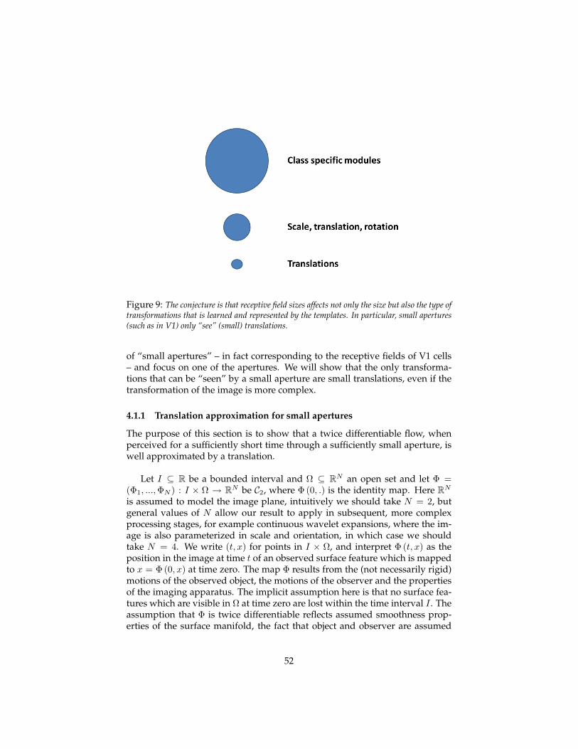
Figure 9: The conjecture is that receptive field sizes affects not only the size but also the type oftransformations that is learned and represented by the templates. In particular, small apertures(such as in V1) only “see” (small) translations.
of “small apertures” – in fact corresponding to the receptive fields of V1 cells– and focus on one of the apertures. We will show that the only transforma-tions that can be “seen” by a small aperture are small translations, even if thetransformation of the image is more complex.
4.1.1 Translation approximation for small apertures
The purpose of this section is to show that a twice differentiable flow, whenperceived for a sufficiently short time through a sufficiently small aperture, iswell approximated by a translation.
Let I ⊆ R be a bounded interval and Ω ⊆ RN an open set and let Φ =(Φ1, ...,ΦN ) : I × Ω → RN be C2, where Φ (0, .) is the identity map. Here RNis assumed to model the image plane, intuitively we should take N = 2, butgeneral values of N allow our result to apply in subsequent, more complexprocessing stages, for example continuous wavelet expansions, where the im-age is also parameterized in scale and orientation, in which case we shouldtake N = 4. We write (t, x) for points in I × Ω, and interpret Φ (t, x) as theposition in the image at time t of an observed surface feature which is mappedto x = Φ (0, x) at time zero. The map Φ results from the (not necessarily rigid)motions of the observed object, the motions of the observer and the propertiesof the imaging apparatus. The implicit assumption here is that no surface fea-tures which are visible in Ω at time zero are lost within the time interval I . Theassumption that Φ is twice differentiable reflects assumed smoothness prop-erties of the surface manifold, the fact that object and observer are assumed
52
massive, and corresponding smoothness properties of the imaging apparatus,including eventual processing.
Now consider a closed ball B ⊂ Ω of radius δ > 0 which models the aper-ture of observation. We may assume B to be centered at zero, and we mayequally take the time of observation to be t0 = 0 ∈ I . Let
Kt = sup(t,x)∈I×B
∥∥∥∥ ∂2
∂t2Φ (t, x)
∥∥∥∥RN
, Kx = supx∈B
∥∥∥∥ ∂2
∂x∂tΦ (0, x)
∥∥∥∥RN×N
.
Here (∂/∂x) is the spatial gradient in RM , so that the last expression is spelledout as
Kx = supx∈B
(N∑l=1
N∑i=1
(∂2
∂xi∂tΦl (0, x)
)2)1/2
.
Of course, by compactness of I × B and the C2-assumption, both Kt and Kx
are finite.
Theorem 4. (Poggio-Maurer) There exists V ∈ RN such that for all (t, x) ∈ I ×B
‖Φ (t, x)− [x+ tV ]‖RN ≤ Kxδ |t|+Ktt2
2.
As one might suspect, the proof reveals this to be just a special case of Taylor’stheorem.
Proof. Denote V (t, x) = (V1, ..., Vl) (t, x) = (∂/∂t) Φ (t, x), V (t, x) =(V1, ..., Vl
)(t, x) =(
∂2/∂t2)
Φ (t, x), and set V := V (0, 0). For s ∈ [0, 1] we have with Cauchy-Schwartz∥∥∥∥ ddsV (0, sx)
∥∥∥∥2
RN=
N∑l=1
N∑i=1
((∂2
∂xi∂tΦl (0, sx)
)xi
)2
≤ K2x ‖x‖2 ≤ K2
xδ2,
whence
‖Φ (t, x)− [x+ tV ]‖
=∥∥∥∥∫ t
0
V (s, x) ds− tV (0, 0)∥∥∥∥
=∥∥∥∥∫ t
0
[∫ s
0
V (r, x) dr + V (0, x)]ds− tV (0, 0)
∥∥∥∥=
∥∥∥∥∫ t
0
∫ s
0
∂2
∂t2Φ (r, x) drds+ t
∫ 1
0
d
dsV (0, sx) ds
∥∥∥∥≤
∫ t
0
∫ s
0
∥∥∥∥ ∂2
∂t2Φ (r, x)
∥∥∥∥ drds+ |t|∫ 1
0
∥∥∥∥ ddsV (0, sx)∥∥∥∥ ds
≤ Ktt2
2+Kx |t| δ.
53
Of course we are more interested in the visible features themselves, than inthe underlying point transformation. If f : RN → R represents these features,for example as a spatial distribution of gray values observed at time t = 0,then we would like to estimate the evolved image f (Φ (t, x)) by a translatef (x+ tV ) of the original f . It is clear that this is possible only under someregularity assumption on f . The simplest one is that f is globally Lipschitz.We immediately obtain the following
Corollary 1. Under the above assumptions suppose that f : RN → R satisfies
|f (x)− f (y)| ≤ c ‖x− y‖
for some c > 0 and all x, y ∈ RN . Then there exists V ∈ RN such that for all(t, x) ∈ I ×B
|f (Φ (t, x))− f (x+ tV )| ≤ c(Kx |t| δ +Kt
t2
2
).
An example As a simple example we take rigid rotation with angular veloc-ity ω about a point v in the image plane, observed in a neighborhood of radiusδ about the origin. Then
Φ (t, x1, x2) =(
cos (ωt) − sin (ωt)sin (ωt) cos (ωt)
)(x1 − v1
x2 − v2
)+(v1
v2
)and with some calculation we obtain the bounds Kt ≤ ω2 (‖v‖+ δ) and Kx ≤√
2 |ω|. The error bound in the theorem then becomes
(‖v‖+ δ)ω2t2/2 +√
2 |ω| tδ.
If we take v = 0, so that the center of rotation is observed , we see that weconsiderably overestimate the true error for large t, but for t → 0 we also seethat we have the right order in δ and that the constant is correct up to
√2.
A one-layer system comprising the full image (a large aperture) would requirea memory-based module to store all the transformations induced by all ele-ments g of the full group of transformations at all ranges. Because this shouldinclude all possible local transformations as well (for instance for an objectwhich is a small part of an image), this quickly becomes computationally infea-sible as a general solution. A hierarchical architecture dealing with small, localtransformations first – which can be assumed to be affine (because of Lemma4) – can solve this problem and may have been evolution’s solution for the ver-tebrate visual system. It is natural that layers with apertures of increasing sizelearn and discount transformations – in a sequence, from local transformationsto more global ones. The learning of transformations during development in asequence of layers with increasing range of invariance corresponds to the termstratification.
54

4.2 Linking conjecture: developmental memory is Hebbian
Summary. Here we introduce the hypothesis that memory of transformations duringdevelopment is Hebbian. Thus instead of storing a sequence of frame of a templatetransforming, synapses store online updates due to the same sequences.
We introduce here a biologically motivated Linking Conjecture: instead ofexplicitly storing a sequence of frames during development as assumed in PartI, we assume that there is Hebbian-like learning at the synapses in visual cortex.The conjecture consists of the following points:
Linking Conjecture
• The memory in a layer of cells (such as simple cells in V1) is stored in theweights of the connections between the neurons and the inputs (from theprevious layers).
• Instead of storing a sequence of discrete frames as assumed in Part I,online learning is more likely, with synaptic weights being incrementallymodified.
• Hebbian-like synapses exist in visual cortex.
• Hebbian-like learning is equivalent to an online algorithm computingPCAs.
• As a consequence, the tuning of simple cortical cells is dictated by thetop PCAs of the templatebook, since Hebbian-like learning such as theOja flow converges to the top PCA.
The algorithm outlined in Part I, in which transformations are “learned”by memorizing sequences of a patch undergoing a transformation, is an algo-rithm similar to the existing HMAX (in which S2 tunings are learned by sam-pling and memorizing random patches of images). Here we study a biologi-cally more plausible online learning rule. Synapses change incrementally af-ter each frame, effectively compressing information contained in the templates
55
and possibly making signatures more robust to noise. Plausible online learn-ing rules for this goal are associative Hebb-like rules which may lead synapsesat the level of simple-complex cells to match their tuning to the eigenvectorsof the templatebooks (Hebb-like are known to be online algorithms for learn-ing the PCA of a set of input patterns). Thus the receptive field at each layerwould be determined by the transformations represented by the complex cellspooling at each layer. Later we will discuss in some detail Oja’s rule[26] as anexample. It is not the only one with the properties we need but it is a sim-ple rule and variations of it are biologically plausible. The key point for nowis that the conjecture links the spectral properties of the transformation beingrepresented in each layer to the spectral properties of the templatebook at eachlevel.
4.2.1 Hebbian synapses and Oja flow
The algorithm outlined in part I in which transformations are “learned” bymemorizing sequences of a patch undergoing a transformation is an algorithmsimilar to the existing HMAX (in which S2 tunings are learned by sampling andmemorizing random patches of images and invariance is hardwired). A bio-logically more plausible online learning rule is somewhat different: synapseswould change as an effect of the inputs, effectively compressing informationcontained in the templates and possibly making signatures more robust tonoise. Plausible online learning rules for this goal are associative Hebbian-likerules. As we will see later, Hebbian-like synaptic rules are expected to lead totuning of the simple cells according to the eigenvectors of the templatebooks.
We discuss here the specific case of the Oja’s flow. Oja’s rule [47, 26] definesthe change in presynaptic weights w given the output response y of a neuronto its inputs to be
∆w = wn+1 −wn = η yn(xn − ynwn) (13)
where is the ”learning rate” and y = wTx. The equation follows from expand-ing to the first order Hebb rule normalized to avoid divergence of the weights.Its continuous equivalent is
w = γ y(x− yw) (14)
Hebb’s original rule, which states in conceptual terms that ”neurons thatfire together, wire together”, is written as ∆w = η y(xn)xn, yielding synapticweights that approach infinity with a positive learning rate. In order for thisalgorithm to actually work, the weights have to be normalized so that eachweight’s magnitude is restricted between 0, corresponding to no weight, and1, corresponding to being the only input neuron with any weight. Mathemati-cally, this requires a modified Hebbian rule:
wi(n+ 1) =wi + η y(x)xi(∑m
j=1[wj + η y(x)xj ]p)1/p
(15)
56

of which Oja’s rule is an approximation.Several theoretical papers on Hebbian learning rules show that selective
changes in synaptic weights are difficult to achieve without building in somehomeostatic or normalizing mechanism to regulate total synaptic strength orexcitability. In the meantime, homeostatic control of synaptic plasticity – corre-sponding to the normalizing term in Oja equation – ([73]) is in fact experimen-tally well established.
The above learning rules converge to the PCA with the largest eigenvalue(see Appendix 24). It is a key conjecture of Part II of this paper that Oja’sflow or some variation of it (with appropriate circuitry), may link the spectralproperties of the templatebook to receptive field tuning in visual areas. Theconjecture is based on Oja’s and other results, summarized by:
Proposition 10. The Oja flow (Equation 13) generates synaptic weights that convergeto the top real eigenvector of the input patterns covariance matrix, that is the covariancematrix of the templatebook (in the noiseless case).
In principle, local invariance to translation can be achieved by averaging afunction over a number of Principal Components for each aperture (ideally all,in practice a small number) corresponding to the “movie” of one transforma-tion sequence. The PCA do in fact span the variability due to the transforma-tion (translation in the case of simple cells): thus this average is equivalent toaveraging over frames of the templatebook, as described in Part I. An empiricalobservation is that most of the PCA for the translation case appear as quadra-ture pairs (this is also true for the other subgroups of the affine group since thecharacters are always Fourier components). It follows that the energy aggrega-tion function is locally invariant (because |eiωnx+θ| = 1) to the transformation(see Figure 18).
In the hypothesis of Oja-type online learning, one possible scenario is thatthat different simple cells which “look” at the same aperture converge to asingle top principal component. Several Oja-like learning rules converge toprincipal components [62, 48]. In the presence of noise, different cells withthe same aperture may converge to different eigenvectors with the same eigen-value (such as the odd and even component of a quadrature pair (see Figure18). A complex cell then aggregates the square or the modulo of two or moresimple cells corresponding to different PCAs. Though diversity in the PCAsto fit the observed RF of simple cells may come from online learning in thepresence of various types of noise, it is much more likely that there is lateralinhibition between nearby simple cells to avoid that they converge to eigen-vectors of the same order (nearby neurons may also be driven by local interac-tion to converge to Gabor-like functions with similar orientation). In addition,Foldiak-type learning mechanisms (see Appendix 24.2) mabe responsible forwiring simple cells with the “same” orientation to the same complex cell.
It has been customary (for instance see [?] to state a single “slowness” max-imization principle, formulated in such a way to imply both Oja’s-like learn-ing at the level of simple cells and wiring of the complex cells according to a
57
Foldiak-like rule. Though such a principle does not seem to reflect any obvi-ous biological plasticity property, it cannot be excluded that a single biologicalmechanisms – as opposed to a single abstract optimization principle – deter-mines both the tuning of the simple cells and their pooling into complex cells.In a similar spirit, simple cells may be a group of inputs on a dendritic branchof a complex cell.
Notice that a relatively small hanges in the Oja equation give an onlinealgorithm for computing ICAs instead of PCAs [23]. Which kind of plasticityis true biologically is an open question. We expect ICAs to be similar to PCAsdescribed here but not identical. Our spectral analysis would not carry overto ICAs – at least not exactly – and instead direct simulations of the dynamiconline equations will have to be done.
Let us summarize the main implications of this section in terms of tem-plates, signatures and simple and complex cells. Notice that the templatebookT is a tensor with τi,j being an array. There are D PCA components for eachT: for instance retaining the first two PCA components shown in Figure 18corresponds to replacing T with T with 2 rows. From this point of view, whatdo we expect it will happen during developmental learning using a Hebb-likerule? Repeated exposure to stimuli sequences corresponding to the rows of theT should induce, through the learning rule, simple cell tunings correspondingfor instance to the two PCA in quadrature pair of Figure 18. Simple cells tunedto these Principal Components would be pooled by the same complex cell.
4.3 Spectral properties of the templatebook covariance opera-tor: cortical equation
Summary. This section focuses on characterizing the spectral properties associatedwith the covariance of the templatebook. It proposes a “cortical equation” whose so-lution provides the eigenfunctions of the covariance. Hebbian synaptic rules implythat during development the tuning of simple cells when exposed to inputs from theretina will converge to the top eigenfunction(s). We start with the 1D analysis; the 2Dproblem is somewhat more interesting because of the “symmetry breaking” induced bymotion.
We consider a layer of 2D “apertures” and the covariance of the template-book associated with each aperture resulting from transformations of images“seen” through one of these apertures. This will lead later to an explicit solu-tion for the first layer in the case of translations.
For any fixed t we want to solve the spectral problem associated to thetemplatebook:
Tt = (g0t, g1t, ..., g|G|t, ....)T
i.e. we want to find the eigenvalues λi and eigenfunctions ψi such that
T∗tTtψi = λiψi, i = 1, ..., N (16)
To state the problem precisely we need some definitions. We start first with the1D problem for simplicity
58

We show how to derive an analytical expression of the visual cortex cellstuning based on the following hypothesis:
1. Observables: images, transforming by a locally compact group, lookedthrough an ”aperture” better specified later.
2. Hebbian learning: hebbian like synapses exists in visual cortex.
We fix few objects:
• X space of signals: L2(C, dx).
• T ⊆ X the template set.
We will solve the eigenproblem associated to the continuous version of (16): inthis case the basic observable given by the operator T : X → X
(TI)(y) ≡ [t ∗MaI](y) =∫
dxt(y − x)a(x)I(x), t ∈ T , a, I ∈ X (17)
where(MaI)(x) = a(x)I(x), a ∈ X
The equation (17) is the mathematical expression of the observable T i.e. atranslating template t looked through the function a which will be called theaperture.
Remark 6. T is linear (from the properties of the convolution operator) and bounded(from ‖T‖ = ‖F(T )‖ = ‖t‖ ‖a‖).Remark 7. Ma is a selfadjoint operator.
The adjoint operator T ∗ : X → X is given by
〈TI, I ′〉 =∫
dy I ′(y)∫
dx t(y − x)a(x)I(x)
=∫
dx I(x)a(x)∫
dy t(y − x)I ′(y) = 〈I, T ∗I ′〉
which implies T ∗I = Ma(t− ∗ I), t−(x) = t(−x). Note that ‖t‖ = ‖t−‖ ⇒‖T‖ = ‖T ∗‖, i.e. ‖T ∗‖ is bounded.Assuming Hebbian learning we have that the tuning of the cortical cells isgiven by the solution of the spectral problem of the covariance operator as-sociated to T , T ∗T : X → X
[T ∗TI](y) = Ma[t− ∗ (t ∗ (MaI))](y) = Ma[(t− ∗ t) ∗ (MaI)](y)
= Ma(t~ ∗ (MaI)) = a(y)∫
dx a(x)t~(y − x)I(x)
The above expression can be written as
[T ∗TI](y) =∫
dx K(x, y)I(x), K(x, y) = a(x)a(y)t~(y − x).
59
Being the kernel K Hilbert-Schmidt, i.e.
Tr(K) =∫
dx K(x, x) =∫
dx a2(x)t~(0) <∞
we have:
• the eigenfunctions corresponding to distinct eigenvalues are orthogonal.
• the eigenvalues are real and positive.
• there is at least one eigenvalues and one eigenfunctions (when K is al-most everywhere nonzero) and in general a countable set of eigenfunc-tions.
In the following paragraphs we aim to find ψn ∈ X and λn ∈ R such that
a(y)∫
dx a(x)t~(y − x)ψn(x) = λnψn(y) (18)
and study their properties. In particular in the next paragraphs we are going tofind approximate solutions and show that they are a Gabor-like wavelets. Anexact solution in some particular cases can be found in the appendix 12.
Remarks
• Square aperture, circulants and FourierWe start from the simplest discrete “toy” case in which we assume pe-riodic boundary conditions on each aperture (one in a layer of receptivefields) resulting on a circulant structure of the templatebook.
Define as templatebook T the circulant matrix where each column rep-resents a template t shifted relative to the previous column. This corre-sponds to assuming that the visual world translates and is “seen througha square aperture” with periodic boundary conditions. Let us assumein this example that the image is one dimensional. Thus the image seenthrough an aperture
a(x) s.t. a(x) = 1 for 0 ≤ x ≤ A and a(x) = 0 otherwise
is t(x−y)a(x) when the image is shifted by y. We are led to the followingproblem: find the eigenvectors of the symmetric matrix TTT where T isa circulant matrix4. If we consider the continuous version of the problem,that is the eigenvalue problem∫ A
0
dxψn(x)t~(y − x)dx = λnψn(y)
with t~(x) being the autocorrelation function associated with t. The so-lution is ψn(x) = e−i2π
nAx which is the Fourier basis between 0 and A.
4This problem has also been considered in recent work from Andrew Ng’s group [63].
60
• Translation invariance of the correlation function of natural images
In the toy example above the two point correlation function t(x, y) hasthe form t(x, y) = t(x − y) because of shifting the vector t. In the caseof natural images, the expected two-point correlation function is alwaystranslation invariant even if the images are sampled randomly [61] (in-stead of being successive frames of a movie). In 1-D there is therefore nodifference between the continuous motion case of one image translatingand random sampling of different natural images (apart signal to noiseissues). As we will see later, sampling from smooth translation is how-ever needed for symmetry breaking of the 2D eigenvalue problem – andthus convergence of the eigenfunctions to directions orthogonal to thedirection of motion.
• The sum of Gaussian receptive fields is constant if their density is large enough
What is∑G(x − ξi)? If
∑G(x − ξi) ≈
∫G(x − ξ)dξ then we know that∫
G(x− ξ)dξ = 1 for normalized G and for −∞ ≤ x ≤ ∞.
4.3.1 Eigenvectors of the covariance of the template book for the translationgroup
As we mentioned, the linking conjecture connect the spectral properties to thetuning of the cells during development. We study here the spectral propertiesof the templatebook.We consider a biologically realistic situation consisting of a layer of Gaussian“apertures”. We characterize the spectral properties of the templatebook asso-ciated with each aperture (corresponding to the receptive field of a “neuron”)resulting from translations of images “seen” through one of these Gaussianapertures. For the neuroscientist we are thinking about a Gaussian distribution(wrt to image space) of synapses on the dendritic tree of a cortical cell in V 1 that willdevelop into a simple cells.
Thus the image seen through a Gaussian aperture is t(x − s)g(x) when theimage is shifted by s. In the discrete case we are led to the following (PCA)problem: find the eigenvectors of the symmetric matrix TTGTGT where G is adiagonal matrix with the values of a Gaussian along the diagonal.
In the following we start with the continuous 1D version of the problem.The 2D version of equation (18) (see remark 9) is an equation describing the
development of simple cells in V 1; we call it “cortical equation” because, as wewill see later, according to the theory it describes development of other corticallayers as well.
Notice that equation (18)∫dxg(y)g(x)ψn(x)t~(y − x) = λnψn(y)
holds for all apertures defined by functions g(x).
61

Figure 10: Continuous spectrum of the covariance of the templatebook: Gabor-like eigenfunc-tions for different σ
Remark 8. Eq. (18) can be easily written in the case x ∈ Y = L2(G, dg) being G alocally compact group
[T ∗TI](g′) =∫
dg K(g, g′)I(g), K(g, g′) = a(g)a(g′)t~(g−1g′), I ∈ Y, g, g′ ∈ G.
The convolution is now on the group G.
Remark 9. In 2D the spectral problem is:∫dξdηg(x, y)g(ξ, η)t~(ξ − x, η − y)ψn(ξ, η) = λnψn(x, y). (19)
where t~ ≡ t~ t.
Numerical simulations in 1D show Gabor-like wavelets (see Figure 10) aseigenfunctions. This result is robust relative to the exact form of the correlationt~(x). Other properties depend on the form of the spectrum (the Fourier trans-form of t~(x)). All the 1D simulations have been made (without any retinalprocessing) directly with natural images – which roughly have t~(ω) ∝ 1
ω2 .In particular, the figures 11, 12 show that (in 1D) the eigenfunctions of the
cortical equation show the key signature of true gabor wavelets in which the fre-quency is proportional to the σ. Figure 13 shows that the Gaussian envelope issmaller than the Gaussian aperture.
The following analysis of the eigenvalue equation provides some intuitionbehind the results of the numerical simulations.
62

Figure 11: Continuous spectrum: λ vs. σα for even symmetric patterns. The slope in thisfigure is k where λ = kσα; k ∼ 2 in this figure.
Figure 12: Continuous spectrum: λ vs. σα for odd symmetric patterns. The slope is ∼ 2.4. In1D, odd symmetric eigenfunctions tend to have a lower modulating frequency.
63
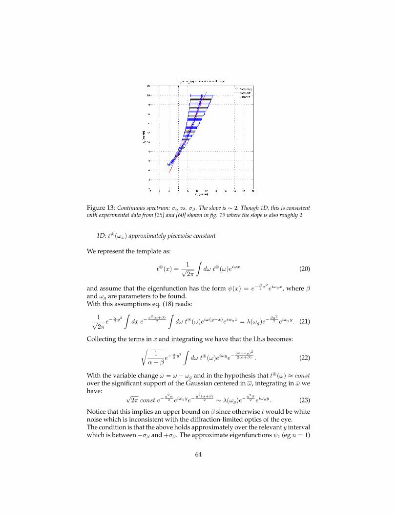
Figure 13: Continuous spectrum: σα vs. σβ . The slope is ∼ 2. Though 1D, this is consistentwith experimental data from [25] and [60] shown in fig. 19 where the slope is also roughly 2.
1D: t~(ωx) approximately piecewise constant
We represent the template as:
t~(x) =1√2π
∫dω t~(ω)eiωx (20)
and assume that the eigenfunction has the form ψ(x) = e−β2 x
2eiωgx, where β
and ωg are parameters to be found.With this assumptions eq. (18) reads:
1√2πe−
α2 y
2∫dx e−
x2(α+β)2
∫dω t~(ω)eiω(y−x)eiwgx = λ(ωg)e−
βy2
2 eiωgy. (21)
Collecting the terms in x and integrating we have that the l.h.s becomes:√1
α+ βe−
α2 y
2∫dω t~(ω)eiωye−
(ω−ωg)2
2(α+β) . (22)
With the variable change ω = ω − ωg and in the hypothesis that t~(ω) ≈ constover the significant support of the Gaussian centered in ω, integrating in ω wehave: √
2π const e−y2α
2 eiωgye−y2(α+β)
2 ∼ λ(ωg)e−y2β
2 eiωgy. (23)
Notice that this implies an upper bound on β since otherwise t would be whitenoise which is inconsistent with the diffraction-limited optics of the eye.The condition is that the above holds approximately over the relevant y intervalwhich is between−σβ and +σβ . The approximate eigenfunctions ψ1 (eg n = 1)
64

has frequency ω0. the minimum value of ω0 is set by the condition thatψ1 has tobe roughly orthogonal to the constant (this assumes that the visual input doeshave a dc component, which implies that there is no exact derivative stage inthe input filtering by the retina).
〈ψ0, ψ1〉 =∫dx e−βx
2e−iω0x, → e−
(ω0)2
β ≈ 0 (24)
Using 2πf0 = 2πλ0
= ω0 the condition above implies e−(2πσβ)λ0
)2 ≈ 0 which can
be satisfied with σβ ≥ λ0; σβ ∼ λ0 is enough since this implies e−(2πσβ)λ0
)2 ≈e−(2π)2
.A similar condition ensures more in general orthogonality of any pair of eigen-functions.∫
dx ψ∗n(x)ψm(x) =∫dxe− x2
σ2β einω0xe−imω0x ∝ e−((m−n)ω0)2σ2
β ,
which gives a similar condition as above. this also implies that λ should in-crease with σ of the Gaussian aperture, which is a property of gabor wavelets!.
2D t~(ωx, ωy) approximately piecewise constant
We represent the template after retinal processing (but without motion) as:
t~(x, y) =1
2π
∫dωxdωyt
~(ωx, ωy)ei(ωxx+ωyy) (25)
and assume the following ansatz: the eigenfunctions have the form ψ(x, y) =e−
β2 x
2e−
γ2 y
2eiωgx, where β, γ and ωg are parameters to be found.
With this assumptions eq. 19 reads:
12πe−
α2 (x2+y2)
∫dξdη e−
ξ2(α+β)2 e−
η2(α+γ)2
∫dωxdωy t
~(ωx, ωy) (26)
eiωx(x−ξ)e−iωyηeiωgξ ξ = λ(ωgx, ω
gy)e−
γ2 y
2e−
βx2
2 eiωgxx (27)
Supposing t~(ωx, ωy) = t~(ωx)t~(ωy) and λ(ωgx, ωgy) = λ(ωgx)λ(ωgy) (which is
the case if the spectrum is piecewise constant) we can separate the integral intothe multiplication of the following two expressions:
1√2πe−
α2 x
2∫dξ e−
ξ2(α+β)2
∫dωx t
~(ωx)eiω(x−ξ)eiωgξ ξ = λ(ωgx)e−
βx2
2 eiωgxx
1√2πe−
α2 y
2∫dη e−
η2(α+γ)2
∫dωy t
~(ωy)e−iωyη = λ(ωgy)e−γ2 y
2
The first equation is exactly the 1D problem analyzed in 4.3.1, meanwhile thesecond is satisfied if γ = α.
Remark 10. note that σy ≤ σα and σy ≤ σx ≤ σα, that is the “receptive fields” areelliptic Gaussians. This prediction is very robust wrt parameters and is clearly verifiedby the experimental data on simple cells across different species.
65
4.4 Retina to V1: processing pipeline
Summary. The image is processed by the retina and the LGN before entering V1.Here we discuss how the spectrum of the image changes because of retinal processing.The main properties of the eigenvectors do not depend on it but some of the importantquantitative properties – such as the linear relation between lambda and σ – do. Thequestion now is: what is the actual spectrum of t during development? Thoughthe main qualitative properties of the eigenvectors of the cortical equation donot depend on it, the quantitative relations do, since the kernel of the inte-gral eigenvalue equation depends on t. In this section we describe models ofprocessing in the retina up to V1 that affect the spectral properties of naturalimages and thereby determine the actual spectrum of t. We should also notethat retinal waves may have a role in the development of cortex (c.f. [79]) inwhich case the spectrum of t during development (or part of development)may be independent of visual images and resemble more the simple case stud-ied above of t = t0 + cos(ωx). It may be possible to expose developing animals– for instance mice – to appropriately controlled artificial t,[15]. It is in any caseinteresting to check what various choice of t may yield.
4.4.1 Spatial and temporal derivatives in the retina
Let us start with the observation that the retina performs both a DOG-like spa-tial filtering operation as well as a high-pass filtering in time, roughly similar toa time derivative, probably to correct the slow signals provided by the photore-ceptors. Natural images have a 1
f spatial spectrum, bandlimited by the opticalpoint spread function at 60 cyclesdegree (in humans). Additional spatial low-pass fil-tering is likely to take place especially during development (in part because ofimmature optics).
This means that the spectrum of the patterns in the templatebook is spa-tially bandpass, likely with a DC component since the DOG derivative-likeoperation is not perfectly balanced in its positive and negative components.The temporal spectrum depends on whether we consider the faster magno orthe slower parvo ganglion cells. The parvo or midget ganglion cells are likely tobe input to the V1 simple cells involved in visual recognition. It is possible thatthe somewhat temporal high-pass properties of the retina and LGN (see [6])simply correct in the direction of motion for the spatially low-pass componentsof the output of the retina (see Figure 14).Consider as input to V1 the result f(x, y; t) of an image i(x, y) with a spatialpower spectrum ∼ 1
ω2 filtered by the combination of a spatial low-pass filterp(ω) and then a bandpass dog. In this simple example we assume that wecan separate a temporal filtering stage with a high-pass impulse response h(t).Thus in the frequency domain
f(ωx, ωy;ωt) ∼ i(ωx, ωy;ωt)p(ωx, ωy)dog(ωx, ωy).
Assume that f(x, y, t) is then filtered through h(t). For example, let us see theimplications of h(t) ∼ d
dt . Consider the effect of the time derivative over the
66

Figure 14: The sequence of processing stage from the retina with spatial low-pass and bandpass(DOG) plus temporal d/dt derivative-like filtering to V1. Thus high-pass temporal filteringcompensates for the spatial blurring in the direction of motion.
signal generated by the translation of an image f(x−vt), where x, v are vectorsin r2:
d Id t
= ∇I · v. (28)
assume for instance that the direction of motion is along the x axis, eg vy = 0.Then
d Id t
=∂I
∂xvx. (29)
Thus the prediction is that motion in the x direction suppresses spatial changesin y, eg spatial frequencies in ωy , and enhances components orthogonal to itsdirection. This means that the time derivative of a pattern with a uniform spa-tial frequency spectrum in a bounded domain ω, as an effect of motion alongx, gives a templatebook with a spectrum in ω which reflects the transformationand not only the spectrum of the image and the filtering of the retina: iωxf(ωx, ωy).Notice that spatial and temporal filtering commute in this linear framework, sotheir order (in the retina) is not important for the analysis. In particular, a highpass time-filtering may exactly compensate for the spatial-low pass operationin the direction of motion (but not in the orthogonal one). Interestingly, this argu-ment is valid not only for translations but for other motions on the plane. From nowon, we assume the pipeline of figure 14. The 2D simulations are performedwith this pipeline using the low-pass filter of Figure 15.
Because of our assumptions, invariances to affine transformations are di-rectly related to actual trajectories inR2 of the image while transforming. Theseare flows on the plane of which a classification exist (see Appendix22). Wehave the following result for the solution of the 2D eigenfunction equation inthe presence of oriented motion:
67

Figure 15: Spatial lowpass filter 1/√ω2x + ω2
y as implemented in the 2D simulations.
Lemma 2. Selection ruleAssume that a templatebook is obtained after the∇2g ∂
∂t filtering of a “video” gener-ated by a transformation which is a subgroup of the affine group Aff(2,R). Then thecomponents in the image spectrum orthogonal to the trajectories of the transformationsare preferentially enhanced.
4.5 Cortical equation: predictions for simple cells in V1
Summary. The numerical simulations predict surprisingly well, almost without anyparameter fitting, quantitative properties of the tuning of simple cells in V1 acrossdifferent species.
Numerical simulations of the cortical equation in 2D using natural imagesmoving in one direction and the pipeline of Figure 14 show that the top eigen-vectors are oriented Gabor-like wavelets. We are mostly interested in the topthree eigenvectors, since they are the ones likely to be relevant as solutions ofa Oja-type equation. Figures 16 and 17 shows that the solutions are very closeto actual Gabor wavelets. A number of other simulations (not shown here) to-gether with the previous theoretical analysis suggests that the Gabor-like formof the solution is robust wrt large changes in the form of the signal spectrum.
Some of the other more quantitative properties however seem to dependon the overall shape of the effective spectrum though in a rather robust way. Inthis respect the simulations agree with the astonishing and little known findingthat data from simple cells in several different species (see Figure 19) show verysimilar quantitative features.
The most noteworthy characteristics of the physiology data are:
• the tuning functions show a λ proportional to σ which is the signature ofwavelets;
68
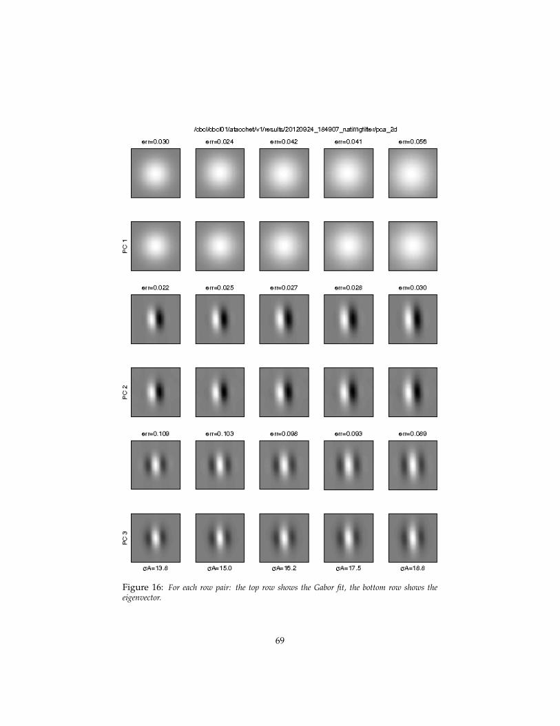
Figure 16: For each row pair: the top row shows the Gabor fit, the bottom row shows theeigenvector.
69

Figure 17: 1D sections of the principal components sorted by eigenvalue (row) for differentGaussian apertures (column). Red indicates best least square fit of a Gabor wavelet.
Figure 18: A vertical slice through a quadrature pair (1st and 2nd eigenvector) from Figure 16.
70
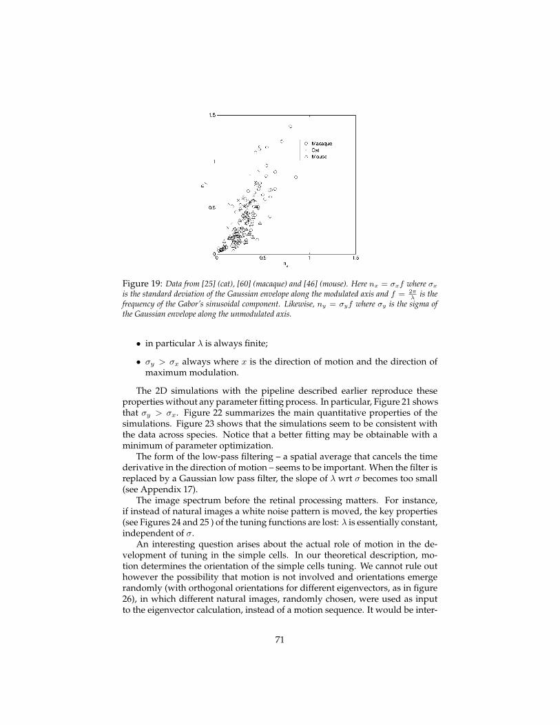
Figure 19: Data from [25] (cat), [60] (macaque) and [46] (mouse). Here nx = σxf where σxis the standard deviation of the Gaussian envelope along the modulated axis and f = 2π
λis the
frequency of the Gabor’s sinusoidal component. Likewise, ny = σyf where σy is the sigma ofthe Gaussian envelope along the unmodulated axis.
• in particular λ is always finite;
• σy > σx always where x is the direction of motion and the direction ofmaximum modulation.
The 2D simulations with the pipeline described earlier reproduce theseproperties without any parameter fitting process. In particular, Figure 21 showsthat σy > σx. Figure 22 summarizes the main quantitative properties of thesimulations. Figure 23 shows that the simulations seem to be consistent withthe data across species. Notice that a better fitting may be obtainable with aminimum of parameter optimization.
The form of the low-pass filtering – a spatial average that cancels the timederivative in the direction of motion – seems to be important. When the filter isreplaced by a Gaussian low pass filter, the slope of λ wrt σ becomes too small(see Appendix 17).
The image spectrum before the retinal processing matters. For instance,if instead of natural images a white noise pattern is moved, the key properties(see Figures 24 and 25 ) of the tuning functions are lost: λ is essentially constant,independent of σ.
An interesting question arises about the actual role of motion in the de-velopment of tuning in the simple cells. In our theoretical description, mo-tion determines the orientation of the simple cells tuning. We cannot rule outhowever the possibility that motion is not involved and orientations emergerandomly (with orthogonal orientations for different eigenvectors, as in figure26), in which different natural images, randomly chosen, were used as inputto the eigenvector calculation, instead of a motion sequence. It would be inter-
71
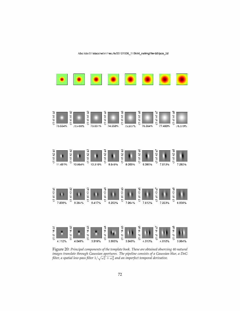
Figure 20: Principal components of the template book. These are obtained observing 40 naturalimages translate through Gaussian apertures. The pipeline consists of a Gaussian blur, a DoGfilter, a spatial low-pass filter 1/
√ω2x + ω2
y and an imperfect temporal derivative.
72
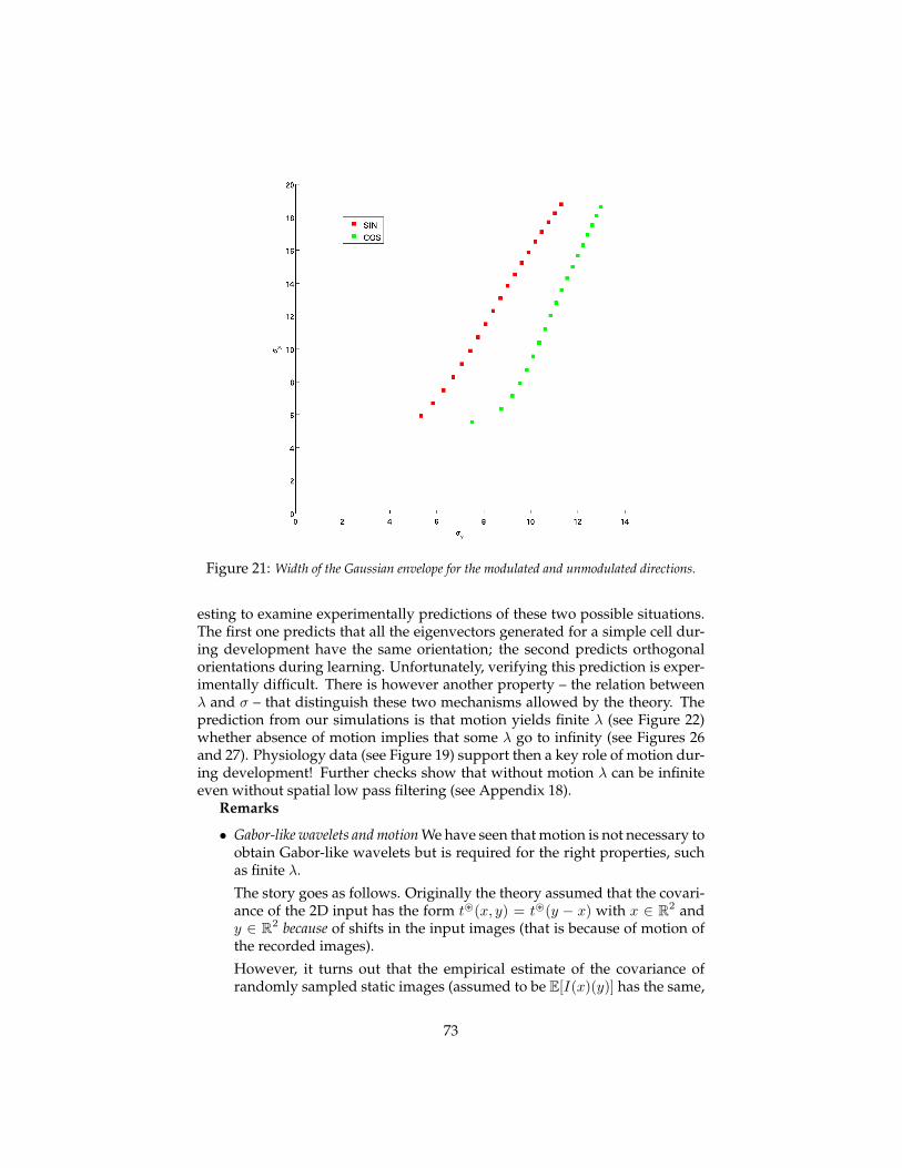
Figure 21: Width of the Gaussian envelope for the modulated and unmodulated directions.
esting to examine experimentally predictions of these two possible situations.The first one predicts that all the eigenvectors generated for a simple cell dur-ing development have the same orientation; the second predicts orthogonalorientations during learning. Unfortunately, verifying this prediction is exper-imentally difficult. There is however another property – the relation betweenλ and σ – that distinguish these two mechanisms allowed by the theory. Theprediction from our simulations is that motion yields finite λ (see Figure 22)whether absence of motion implies that some λ go to infinity (see Figures 26and 27). Physiology data (see Figure 19) support then a key role of motion dur-ing development! Further checks show that without motion λ can be infiniteeven without spatial low pass filtering (see Appendix 18).
Remarks
• Gabor-like wavelets and motion We have seen that motion is not necessary toobtain Gabor-like wavelets but is required for the right properties, suchas finite λ.
The story goes as follows. Originally the theory assumed that the covari-ance of the 2D input has the form t~(x, y) = t~(y − x) with x ∈ R2 andy ∈ R2 because of shifts in the input images (that is because of motion ofthe recorded images).
However, it turns out that the empirical estimate of the covariance ofrandomly sampled static images (assumed to be E[I(x)(y)] has the same,
73
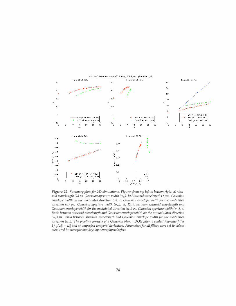
Figure 22: Summary plots for 2D simulations. Figures from top left to bottom right: a) sinu-soid wavelength (λ) vs. Gaussian aperture width (σα). b) Sinusoid wavelength (λ) vs. Gaussianenvelope width on the modulated direction (σ). c) Gaussian envelope width for the modulateddirection (σ) vs. Gaussian aperture width (σα). d) Ratio between sinusoid wavelength andGaussian envelope width for the modulated direction (nx) vs. Gaussian aperture width (σα). e)Ratio between sinusoid wavelength and Gaussian envelope width on the unmodulated direction(ny) vs. ratio between sinusoid wavelength and Gaussian envelope width for the modulateddirection (nx). The pipeline consists of a Gaussian blur, a DOG filter, a spatial low-pass filter1/√ω2x + ω2
y and an imperfect temporal derivative. Parameters for all filters were set to valuesmeasured in macaque monkeys by neurophysiologists.
74

Figure 23: This figure shows the σ/λ ratio for the modulated and unmodulated direction of theGabor wavelet. Neurophysiology data from monkeys, cats and mice are reported together withour simulations
75
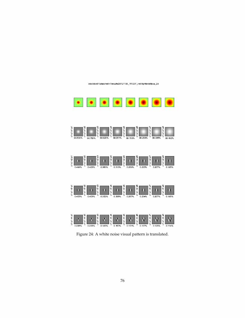
Figure 24: A white noise visual pattern is translated.
76
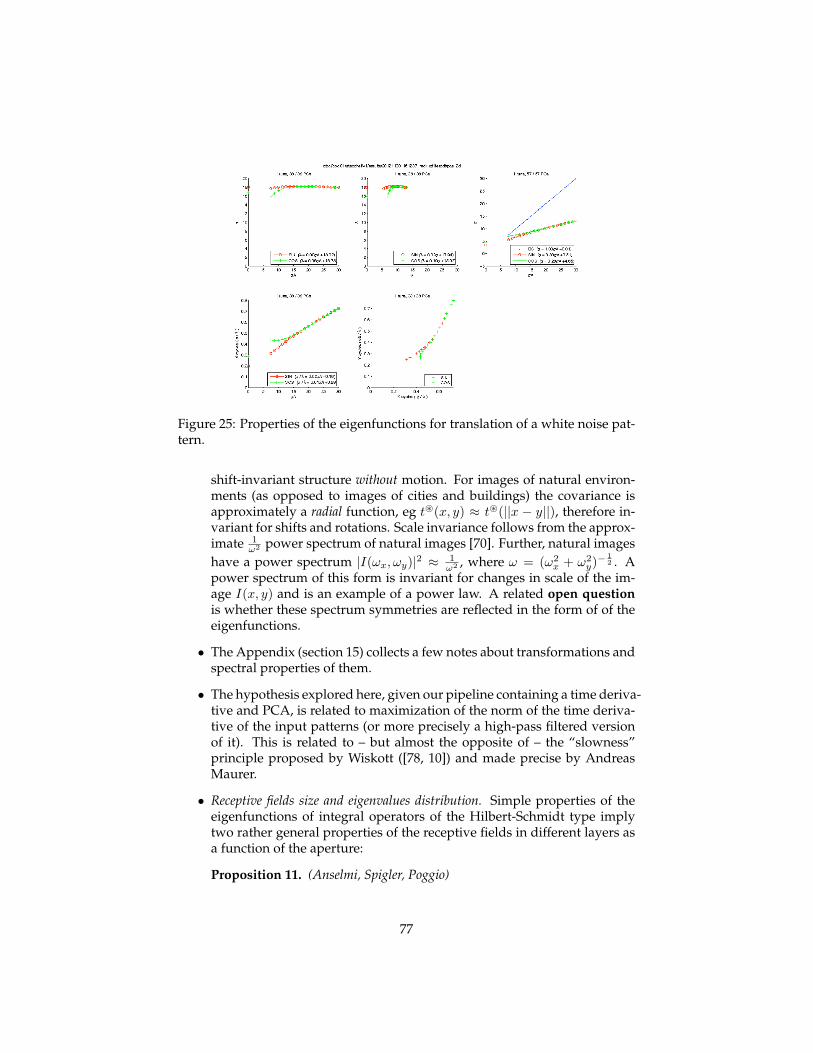
Figure 25: Properties of the eigenfunctions for translation of a white noise pat-tern.
shift-invariant structure without motion. For images of natural environ-ments (as opposed to images of cities and buildings) the covariance isapproximately a radial function, eg t~(x, y) ≈ t~(||x − y||), therefore in-variant for shifts and rotations. Scale invariance follows from the approx-imate 1
ω2 power spectrum of natural images [70]. Further, natural imageshave a power spectrum |I(ωx, ωy)|2 ≈ 1
ω2 , where ω = (ω2x + ω2
y)−12 . A
power spectrum of this form is invariant for changes in scale of the im-age I(x, y) and is an example of a power law. A related open questionis whether these spectrum symmetries are reflected in the form of of theeigenfunctions.
• The Appendix (section 15) collects a few notes about transformations andspectral properties of them.
• The hypothesis explored here, given our pipeline containing a time deriva-tive and PCA, is related to maximization of the norm of the time deriva-tive of the input patterns (or more precisely a high-pass filtered versionof it). This is related to – but almost the opposite of – the “slowness”principle proposed by Wiskott ([78, 10]) and made precise by AndreasMaurer.
• Receptive fields size and eigenvalues distribution. Simple properties of theeigenfunctions of integral operators of the Hilbert-Schmidt type implytwo rather general properties of the receptive fields in different layers asa function of the aperture:
Proposition 11. (Anselmi, Spigler, Poggio)
77

Figure 26: Eigenvectors of covariance matrix of scrambled set of images (sameas in Figure 16 but scrambled). There is no continuous motion. The orientationof wavelets changes.
78

Figure 27: As in the previous Figure. λ can be infinite since orthogonality wrtto lower order eigenfunction is ensured by orthogonal orientation.
79

Figure 28: Eigenvalues behavior as a function of the aperture for general Hilbert-Schmidtintegral operators.
– Under the assumption of a power spectrum of the form t(ω) ∝ 1ω2 , the
eigenvalues obey the relation:
λi(σ)λi(σ)
≥ 1, σ ≥ σ.
This suggests that the top eigenvalues are closer to each other for largeapertures, suggesting that in the presence of noise the eigenvector emergingas the result of Oja’s flow may vary among the several top eigenvectors.
– The number of eigenfunctions depends on the size of the receptive field: thisalso suggests that the variety of tunings increases with the size of the RFs.
4.6 Complex cells: wiring and invariance
Summary.We show that local PCA can substitute for templates in the sense that groupaverages over nonlinear functions of the PCA may be invariant. This is true in partic-ular for modulo square nonlinearities. The section analyzes the connection between thesimple complex cells stage of our theory with the first iteration of Mallat’s scatteringtransform [42].
In the theory, complex cells are supposed to pool nonlinear functions of(shifted) templates over a small bounded domain in x, y, representing a par-tial group average. Clearly, pooling the modulo square of the top Gabor-likeeigenvectors over a x, y domain is completely equivalent (since the eigenvec-tors are legitimate templates). Interestingly, pooling the modulo square of thetop Gabor-like wavelets is also equivalent to a partial group average over a(small) domain. This can be seen (and proven) in a number of ways. Theintuition is that the Gabor-like eigenvectors capture the transformations seen
80
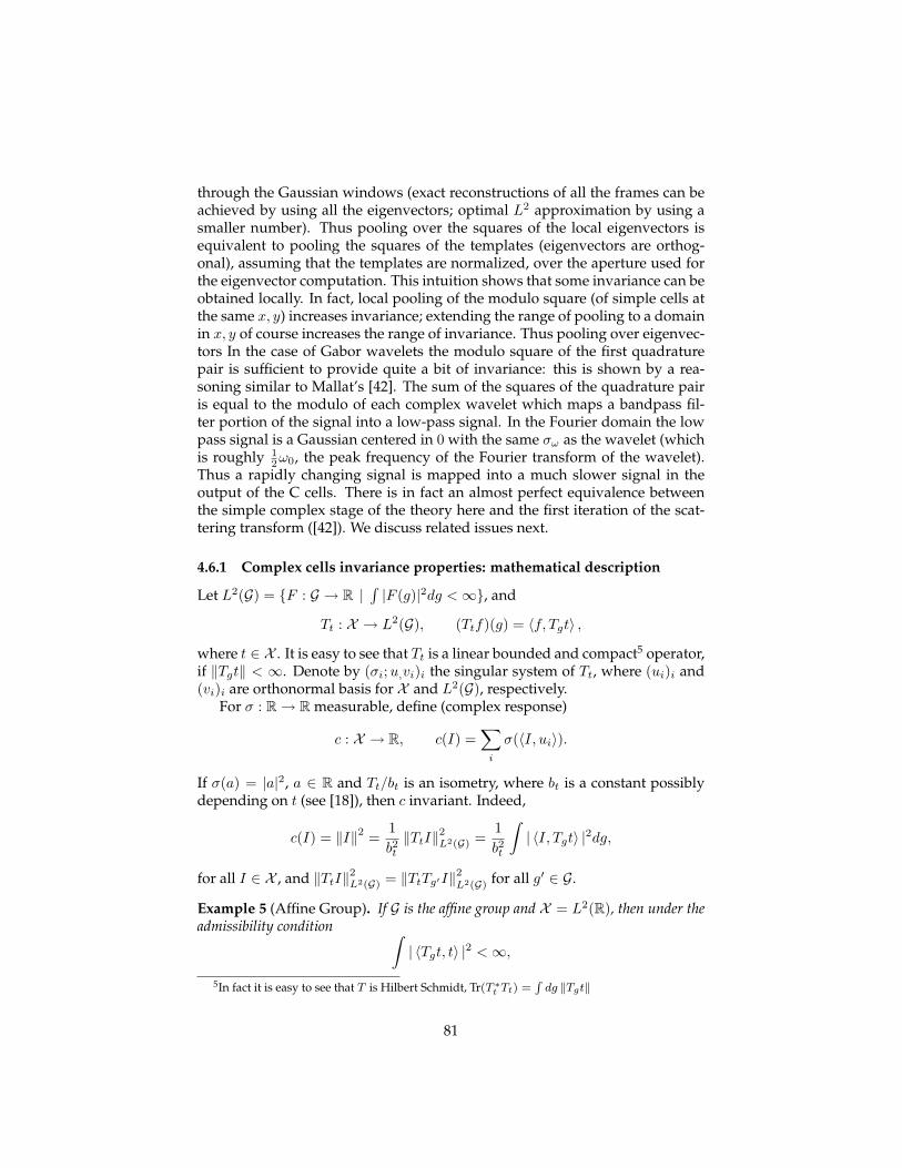
through the Gaussian windows (exact reconstructions of all the frames can beachieved by using all the eigenvectors; optimal L2 approximation by using asmaller number). Thus pooling over the squares of the local eigenvectors isequivalent to pooling the squares of the templates (eigenvectors are orthog-onal), assuming that the templates are normalized, over the aperture used forthe eigenvector computation. This intuition shows that some invariance can beobtained locally. In fact, local pooling of the modulo square (of simple cells atthe same x, y) increases invariance; extending the range of pooling to a domainin x, y of course increases the range of invariance. Thus pooling over eigenvec-tors In the case of Gabor wavelets the modulo square of the first quadraturepair is sufficient to provide quite a bit of invariance: this is shown by a rea-soning similar to Mallat’s [42]. The sum of the squares of the quadrature pairis equal to the modulo of each complex wavelet which maps a bandpass fil-ter portion of the signal into a low-pass signal. In the Fourier domain the lowpass signal is a Gaussian centered in 0 with the same σω as the wavelet (whichis roughly 1
2ω0, the peak frequency of the Fourier transform of the wavelet).Thus a rapidly changing signal is mapped into a much slower signal in theoutput of the C cells. There is in fact an almost perfect equivalence betweenthe simple complex stage of the theory here and the first iteration of the scat-tering transform ([42]). We discuss related issues next.
4.6.1 Complex cells invariance properties: mathematical description
Let L2(G) = F : G → R | ∫ |F (g)|2dg <∞, and
Tt : X → L2(G), (Ttf)(g) = 〈f, Tgt〉 ,where t ∈ X . It is easy to see that Tt is a linear bounded and compact5 operator,if ‖Tgt‖ < ∞. Denote by (σi;u,vi)i the singular system of Tt, where (ui)i and(vi)i are orthonormal basis for X and L2(G), respectively.
For σ : R→ Rmeasurable, define (complex response)
c : X → R, c(I) =∑i
σ(〈I, ui〉).
If σ(a) = |a|2, a ∈ R and Tt/bt is an isometry, where bt is a constant possiblydepending on t (see [18]), then c invariant. Indeed,
c(I) = ‖I‖2 =1b2t‖TtI‖2L2(G) =
1b2t
∫| 〈I, Tgt〉 |2dg,
for all I ∈ X , and ‖TtI‖2L2(G) = ‖TtTg′I‖2L2(G) for all g′ ∈ G.
Example 5 (Affine Group). If G is the affine group and X = L2(R), then under theadmissibility condition ∫
| 〈Tgt, t〉 |2 <∞,5In fact it is easy to see that T is Hilbert Schmidt, Tr(T ∗t Tt) =
∫dg ‖Tgt‖
81

it is possible to take bt =√Ct, with Ct = 2π
∫ |t(ω)|2ω dω, where t denotes the Fourier
transform of t.
4.6.2 Hierarchical frequency remapping
The theory so far does not provide information about the size of the receptivefields for the first layer S and C cells. Here we sketch an approach to thisquestion which is related to section 9.4. A main difference is that we considerhere the specific case of templates being Gabor wavelets and of pooling beingenergy pooling over a bounded interval. Thus we consider a partial groupaverage of the squares.
We begin by considering one dimensional “images”. Let the image I(x) ∈X . To analyze I(x) we use a wavelet centered in ω0, x ∗ ψω0,σ0
where σ0 isthe width σ1s of the wavelet Gaussian envelope, that is of the envelope of thesimple cells impulse response at fist layer. There are several such channels cen-tered on different frequencies and with corresponding σ resulting from Heb-bian learning as described in previous sections such as 4.4.1. As an examplethe highest frequency channel may be centered on a frequency ω0 that satisfiesωmax ≤ ω0 + 3σ0 with max(supp(I)) = ωmax.
The signal I can be reconstructed exactly – apart from its DC and low fre-quencies around it – by combining a sufficiently large number of such bandpassfilters according to the identity
∫G(ω − ω′)dω′I(ω) = I(ω).
The pooling operation, from simple to complex cells, starts with taking themodulus square of the wavelet filtered signal. In Fourier space, the operationmaps the support of the Fourier transform of I ∗ ψω0,σ0
into one interval, cen-tered in 0.
A one-octave bandwidth – that we conjecture is the maximum still yield-ing full information with a low number of bits (see Appendix 11.1)) – impliesa certain size of the receptive field (see above) of simple cells. Complex cellspreserve information about the original image if the pooling region is in the or-der of the support of the simple cells (thus in the order of 6σ), since we assumethat the sign of the signal is known (positive and negative parts of the signalare carried by different neural channels, see Appendix 11.1). The same reason-ing can be also applied to higher order simple cells learned on the 4-D cube(see later) to obtain estimates of RF size at a fixed eccentricity. Interestingly,these arguments suggest that if information is preserved by pooling (which isnot necessary in our case), then there the C cells pooling regions are very small(in order of
√2 the simple cells receptive fields): most of the invariance is then
due to the RF of simple cells and the pooling effect of the modulo square (sumover quadrature pairs).
4.7 Beyond V1
Summary. We show that the V1 representation – in terms of Gabor-like wavelets inx, y, θ, s – can locally approximate (within balls of radius r with r
R ≤ δ where R is
82

the retinal eccentricity) similitude transformations of the image as independent shiftsin a 4-dimensional space (The subgroup of translations is a 2-parameter group (trans-lations in x, y); the subgroup of rotations and dilations is also a two parameters group(ρ, θ)). Thus learning on the V1 representation generates 4-dimensional wavelets. Theprediction seems consistent with physiology data. Assuming that R is retinal eccen-tricity corresponds to assuming that most of the experienced and learned “rotationsand looming are centered in the fovea.
4.7.1 Almost-diagonalization of non commuting operators
Let us start from the fact that if (ei, i = 1, ..., N) is an orthonormal basis in anyfinite Hilbert space, the matrix whose entries are ai,j = 〈Aei, ej〉 is diagonal ifand only if each ei is an eigenfunction of the operator A:
ai,j = 〈Aei, ej〉 = λi 〈ei, ej〉 = λiδi,j
If another operator B acting on the Hilbert space is such that [A,B] = 0 thetwo operators share the same eigenfunctions and can therefore be simultane-ously diagonalize. For example in the case of the Fourier basis eixω we cansay that the Fourier transform diagonalize any operator that commutes withtranslation.What can we say if we have two commuting operators, A,B? In this case wecannot have simultaneous diagonalization but choosing a basis ei of the Hilbertspace we have
〈Aei, ej〉 = ai,j + ∆(A)i,j〈Bei, ej〉 = bi,j + ∆(B)i,j .
since the eigenvalues (the measurement results) cannot be determined withinfinite precision at the same time. In this case we can speak of almost si-multaneous diagonalization of the operators A,B if there exists a basis ψi thatminimize simultaneously ∆(A)i,j ,∆(B)i,j , i 6= j. This corresponds to find theset of functions ψ that minimize the uncertainty principle
(∆ψA)(∆ψB) ≥ 12|[A,B]ψ|
Example 6. The Weyl-Heisenberg group in one dimension is generated by two noncommuting operators, the translation in frequency and space. The minimizers of theassociated uncertainty relations gives Gabor functions as solutions.
Example 7. The affine group in dimension two...
4.7.2 Independent shifts and commutators
(From [9])
83
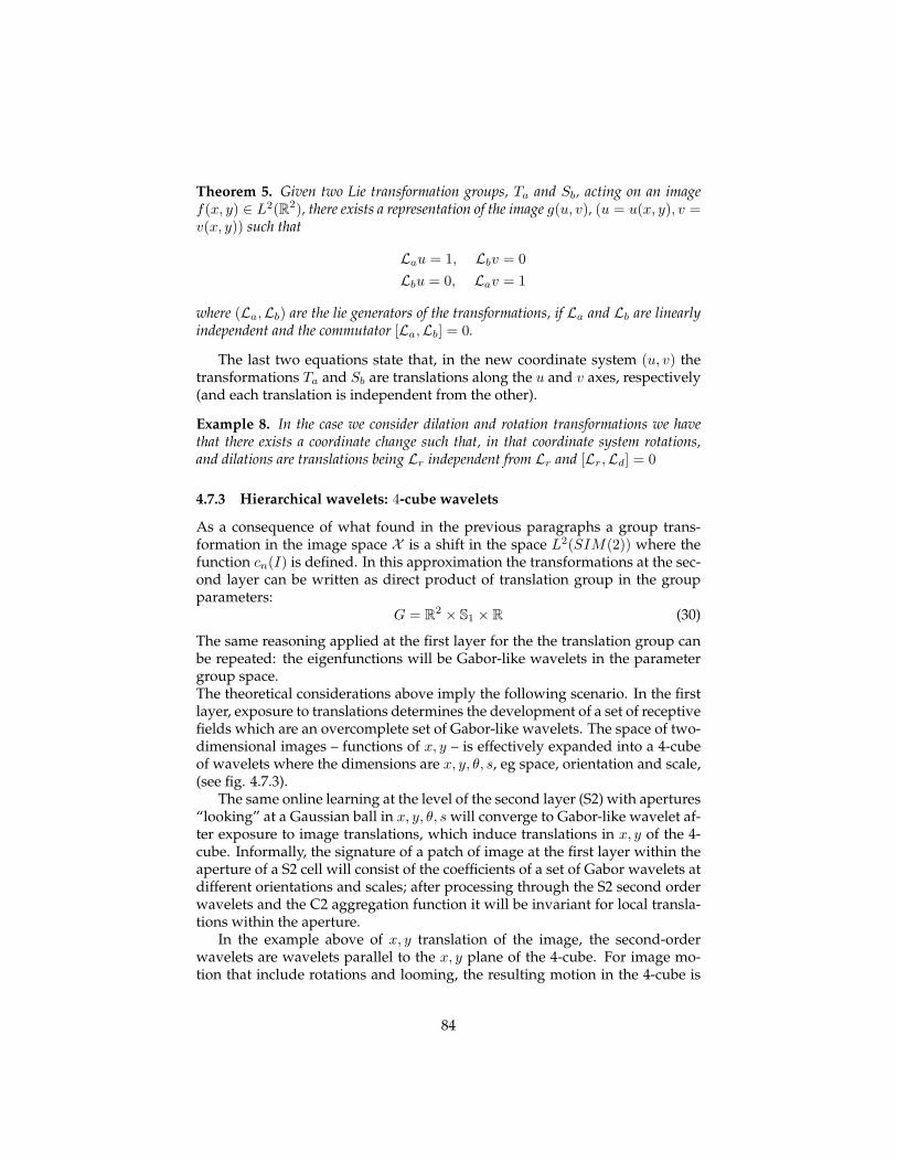
Theorem 5. Given two Lie transformation groups, Ta and Sb, acting on an imagef(x, y) ∈ L2(R2), there exists a representation of the image g(u, v), (u = u(x, y), v =v(x, y)) such that
Lau = 1, Lbv = 0Lbu = 0, Lav = 1
where (La,Lb) are the lie generators of the transformations, if La and Lb are linearlyindependent and the commutator [La,Lb] = 0.
The last two equations state that, in the new coordinate system (u, v) thetransformations Ta and Sb are translations along the u and v axes, respectively(and each translation is independent from the other).
Example 8. In the case we consider dilation and rotation transformations we havethat there exists a coordinate change such that, in that coordinate system rotations,and dilations are translations being Lr independent from Lr and [Lr,Ld] = 0
4.7.3 Hierarchical wavelets: 4-cube wavelets
As a consequence of what found in the previous paragraphs a group trans-formation in the image space X is a shift in the space L2(SIM(2)) where thefunction cn(I) is defined. In this approximation the transformations at the sec-ond layer can be written as direct product of translation group in the groupparameters:
G = R2 × S1 × R (30)
The same reasoning applied at the first layer for the the translation group canbe repeated: the eigenfunctions will be Gabor-like wavelets in the parametergroup space.The theoretical considerations above imply the following scenario. In the firstlayer, exposure to translations determines the development of a set of receptivefields which are an overcomplete set of Gabor-like wavelets. The space of two-dimensional images – functions of x, y – is effectively expanded into a 4-cubeof wavelets where the dimensions are x, y, θ, s, eg space, orientation and scale,(see fig. 4.7.3).
The same online learning at the level of the second layer (S2) with apertures“looking” at a Gaussian ball in x, y, θ, s will converge to Gabor-like wavelet af-ter exposure to image translations, which induce translations in x, y of the 4-cube. Informally, the signature of a patch of image at the first layer within theaperture of a S2 cell will consist of the coefficients of a set of Gabor wavelets atdifferent orientations and scales; after processing through the S2 second orderwavelets and the C2 aggregation function it will be invariant for local transla-tions within the aperture.
In the example above of x, y translation of the image, the second-orderwavelets are wavelets parallel to the x, y plane of the 4-cube. For image mo-tion that include rotations and looming, the resulting motion in the 4-cube is
84

Figure 29: Learning an S2 filter from C1 outputs (of a single scale only). Here the transfor-mation is off-center rotation. The resulting S2 filters are Gabor filters in 3 dimensions: x; y, andorientation. Left: the receptive field center is in the middle (central blue asterisk) but the center ofrotation is to the left (green asterisk). The green arrows show the speed of optical flow at variousplaces. Middle: the learned filters. Each row represents a single filter; since the filters are 3D,we show a separate (x, y) plane for each orientation. However, in this view it is not easy to seeshifting along the orientation dimension. Right: here we show that the 3D Gabors also have asinusoidal component along the orientation dimension. We show a single slice, at the central Xposition, for each filter. The slices are planes in (y, orientation).
85
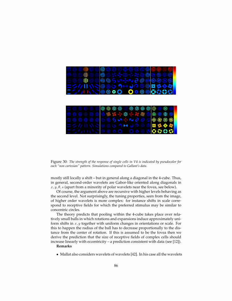
Figure 30: The strength of the response of single cells in V4 is indicated by pseudocolor foreach “non cartesian” pattern. Simulations compared to Gallant’s data.
mostly still locally a shift – but in general along a diagonal in the 4-cube. Thus,in general, second-order wavelets are Gabor-like oriented along diagonals inx, y, θ, s (apart from a minority of polar wavelets near the fovea, see below).
Of course, the argument above are recursive with higher levels behaving asthe second level. Not surprisingly, the tuning properties, seen from the image,of higher order wavelets is more complex: for instance shifts in scale corre-spond to receptive fields for which the preferred stimulus may be similar toconcentric circles.
The theory predicts that pooling within the 4-cube takes place over rela-tively small balls in which rotations and expansions induce approximately uni-form shifts in x, y together with uniform changes in orientations or scale. Forthis to happen the radius of the ball has to decrease proportionally to the dis-tance from the center of rotation. If this is assumed to be the fovea then wederive the prediction that the size of receptive fields of complex cells shouldincrease linearly with eccentricity – a prediction consistent with data (see [12]).
Remarks
• Mallat also considers wavelets of wavelets [42]. In his case all the wavelets
86

are in x, y only with orientation and scale as parameters, whereas in thesimple cells of V2 or higher we expect wavelets on x, y, orientation andscale.
• V 1 (may be with V 2) diagonalize the affine group: how can we check thisprediction?
4.7.4 Predictions for V2, V4, IT
If during learning gaze is precisely maintained, then neurons which happento contain the center of rotation and looming could develop wavelets in polarcoordinates. The probability of this occurring is probably very low for any ofthe small receptive fields in V1 but could be considerably higher for the largerreceptive fields in areas such as V4—close to the very center of the fovea. Inother words, in V2 and especially V4, some of the larger receptive fields couldcontain the center of rotation or the focus of expansion. The correspondingwavelets would be a mix of shifts in orientation and non-uniform translationsin x, y (circles around the center of rotation) with respect to the previous layer.We expect quite a variety of wavelets – once projected back in image space.This could explain variety of receptive fields seen in Gallant’s results [14].
87

Shape Processing in V2 vs. V4* Hegdé and Van Essen
14
to V2. The percentage of cells responding better to complex contours than to bars was 87% for V4 and 84% for V2, and the percentage for which this preference was significant was 36% for V4 and 37% for V2.
Together, the above results suggest that the differences between V2 and V4 populations in their preferences for complex shapes are modest and are outweighed by the similarities. Notably, the differences did not involve systematically greater preferences for more complex stimuli in V4 compared to V2.
Figure 5. The effectiveness of the various stimulus subclasses for V4 vs. V2. Each cell from either area was classified according the subclass to which its most effective grating or contour stimulus belonged. The resulting distributions are shown here for grating stimuli (panel A) or contour stimuli (panel B) for both V4 (top row) and V2 (bottom row; reformatted from Fig. 2 of Hegdé and Van Essen, 2000). In each case, the filled bars denote cells for which the response to its most effective grating/contour stimulus was significantly larger than its response to the second most effective grating/contour stimulus. The stimulus subclasses for which the actual proportion of cells significantly differed from the proportion expected from a uniform distribution at p < 0.05 (single asterisk) or at p < 0.01 (double asterisks) as determined by the binomial proportions test are shown. The cases where the absence of filled bars was statistically significant are denoted by asterisks in black boxes above the corresponding bars. Note that the tests of significance were performed using raw numbers, not percentages, although the data are plotted as percentages in this figure (and in subsequent figures where appropriate) to facilitate comparisons between the areas, all of which had different sample sizes. In this and subsequent figures where appropriate, the exemplar cells in Figure 3A-D are denoted by the corresponding letters.
Figure 31: The effectiveness of the various stimulus subclasses for V4 vs. V2. Each cell fromeither area was classified according the subclass to which its most effective grating or contourstimulus belonged. The resulting distributions are shown here for grating stimuli (panel A) orcontour stimuli (panel B) for both V4 (top row) and V2. See [19].
88
5 Part III: Class-specific transformations and mod-ularity
5.1 Approximate invariance to non-generic transformations
Affine transformations are generic—invariance to them can be learned fromany template objects and applied to any test objects. Many other importanttransformations do not have this property. Non-generic transformations de-pend on information that is not available in a single image. Perfect invarianceto non-generic transformations is not possible. However, approximate invari-ance can still be achieved as long as the template objects transform similarly tothe test objects. One view of this is to say that the missing information in the ob-ject’s 2D projection is similar between template and test objects. For example,3D rotation is a non-generic transformation—as a map between projected 2Dimages it depends on the object’s 3D structure. If the template and test objectshave the same 3D structure then the transformation learned on the templatewill apply exactly to the test object. If they differ in 3D structure then the errorincurred is a function of the difference between their 3D structures.
Many non-generic transformations are class-specific. That is, there is a classof objects that are similar enough to one another that good (approximate) in-variance can be achieved for new instances of the class by pooling over tem-plates of the same type. Faces are the prototypical example of objects that havemany class-specifc transformations. Faces are all similar enough to one an-other that prior knowledge of how a small set of faces transform can be used torecognize a large number of new faces invariantly to non-generic transforma-tions like 3D rotations or illumination changes. We can extend our notion of anon-generic transformation even further and consider transformations that aredifficult to parameterize like facial expressions or aging.
5.2 3D rotation is class-specific
There are many non-generic transformations. As an illustrative example weconsider 3D rotation and orthographic projection along the z-axis of 3-spacewith the center of projection Cp at the origin (see figure 32). In homogenouscoordinates this projection is given by
P =
1 0 0 00 1 0 00 0 0 1
(31)
In 3D homogenous coordinates a rotation around the y-axis is given by
Rθ =
cos(θ) 0 sin(θ) 0
0 1 0 0− sin(θ) 0 cos(θ) 0
0 0 0 1
(32)
89
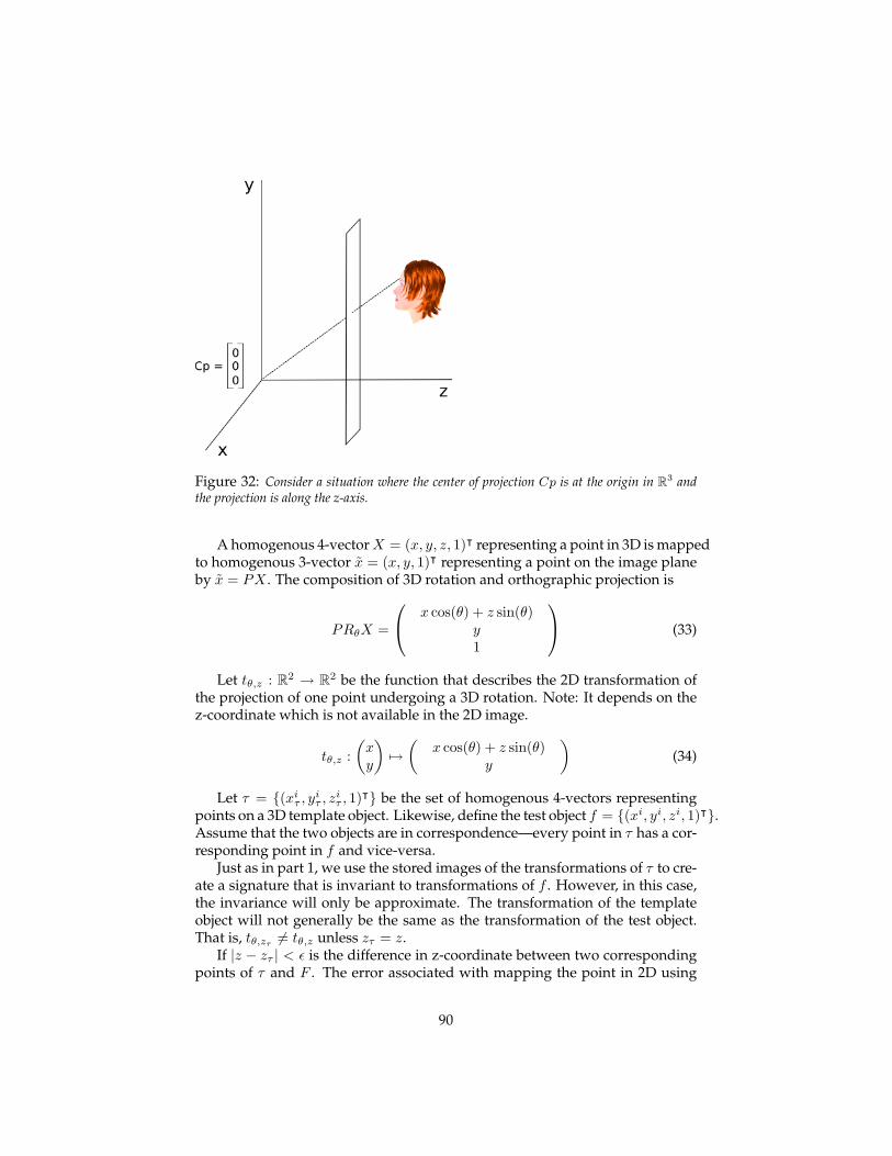
Figure 32: Consider a situation where the center of projection Cp is at the origin in R3 andthe projection is along the z-axis.
A homogenous 4-vectorX = (x, y, z, 1)ᵀ representing a point in 3D is mappedto homogenous 3-vector x = (x, y, 1)ᵀ representing a point on the image planeby x = PX . The composition of 3D rotation and orthographic projection is
PRθX =
x cos(θ) + z sin(θ)y1
(33)
Let tθ,z : R2 → R2 be the function that describes the 2D transformation ofthe projection of one point undergoing a 3D rotation. Note: It depends on thez-coordinate which is not available in the 2D image.
tθ,z :(xy
)7→(
x cos(θ) + z sin(θ)y
)(34)
Let τ = (xiτ , yiτ , ziτ , 1)ᵀ be the set of homogenous 4-vectors representingpoints on a 3D template object. Likewise, define the test object f = (xi, yi, zi, 1)ᵀ.Assume that the two objects are in correspondence—every point in τ has a cor-responding point in f and vice-versa.
Just as in part 1, we use the stored images of the transformations of τ to cre-ate a signature that is invariant to transformations of f . However, in this case,the invariance will only be approximate. The transformation of the templateobject will not generally be the same as the transformation of the test object.That is, tθ,zτ 6= tθ,z unless zτ = z.
If |z − zτ | < ε is the difference in z-coordinate between two correspondingpoints of τ and F . The error associated with mapping the point in 2D using
90

tθ,zτ instead of tθ,z is given by
‖tθ,z(xy
)− tθ,zτ
(xy
)‖ < (ε sin(θ))2 (35)
5.2.1 The 2D transformation
So far this section has only been concerned with 3D transformations of a singlepoint. We are actually interested in the image induced by projecting a 3D object(a collection of points). We define the rendering operator Pq[f ] that takes a set ofhomogenous points in 3D and a texture vector q and returns the image map thatputs the corresponding gray value at each projected point.
Definition: Let f = (xi, yi, zi, 1)ᵀ be a set of N homogenous 4-vectorsrepresenting points on a 3D object. Use the notation f i to indicate the i-thelement of f . Let q ∈ RN with qi ∈ [0, 1] for i = 1, ..., N be the vector of texturevalues for each point of f . Let P be the orthographic projection matrix. Definethe map Pq[f ] : R2 → R such that ∀v ∈ R2:
Pq[f ](v) =
qi if v = Pf i
0 otherwise(36)
Remark 1: This definition of the rendering function assumes uniform light-ing conditions. To address the general case that would allow for variationsin gray value over the rendered image arising from the lighting direction thisfunction would also have to depend on the object’s material properties as wellas other properties of the scene’s lighting.
Remark 2: This definition leaves ambiguous the case where more than onepoint of the object projects to the same point on the image plane (the case wherePf i = Pf j for some i 6= j). For now we assume that we are only consideringobjects for which this does not happen. We will have additional comments onthe case where self-occlusions are allowed below.
Analogously to the single point case, we can write the 2D transformationTθ,~z : L2(R2) → L2(R2) that maps an image of a 3D object to its image after a3D rotation. It depends on a vector of parameters ~z ∈ RN .
Tθ,~z[Pq[f ]] = Pq[Rθgi : i = 1, ..., N] (37)
Where gi is obtained by replacing the z-component of f i with ~zi. Thus
Tθ,~z[Pq[f ]] = Pq[Rθf i : i = 1, ..., N] if ~zi = the z-component of f i (∀i)(38)
Tθ,~z transforms individual points in the following way:
Tθ,~z[Pq[f ]](xy
)= Pq[f ]
(x cos(θ) + z sin(θ)
y
)(39)
91

We can bound the error arising from mapping the image using ~zτ obtainedfrom a template object τ = (xiτ , yiτ , ziτ , 1)ᵀ—different from the test object f .
If |ziτ − zif | < ε (∀i) then
‖Tθ, ~zτ [Pq[f ]]−Pq[Rθf i : i = 1, ..., N]‖ < ΣNi=1|ziτ sin(θ)−zif sin(θ)|2 = N(ε sin(θ))2
(40)
5.2.2 An approximately invariant signature for 3D rotation
We now consider a range of transformations Tθ, ~zτ for θ ∈ [−π, π]. As in part1 we define the template response (the S-layer response) as the normalized dotproduct of an image with all the transformations of a template image.
∆Tθ, ~zτ ,Pq [τ ](Pq[f ]) =
< T−π, ~zτ [Pq[τ ]] , Pq[f ] >...
< Tπ, ~zτ [Pq[τ ]] , Pq[f ] >
(41)
In the affine case we have that ∆G,τ (f) = ∆G,f (τ) up to the ordering of theelements. In that case this fact implies that the signature is invariant.
However, in the case of 3D rotation/projection the template response isdefined with respect to the 2D transformation that uses the parameters ~zτ ob-tained from the z-coordinates of τ . Therefore the analogous statement to theinvariance lemma of part 1 is false.
In the case of 3D rotation / projection there is only approximate invariance.How close of an approximation it is depends on to what extent the templateand test object share 3D structure. We have the following statement.
If for all stored views of the template τ , the difference between the z-coordinate ofeach point and its corresponding point in the test object f is less than ε. That is, if
|ziτ − zif | < ε (∀i). (42)
Then there exists a permutation function S such that
S(∆Tθ, ~zτ ,Pq [τ ](Pq[f ]))−∆Tθ, ~zτ ,Pq [f ](Pq[τ ]) < N(ε sin(θ))2~1 (43)
This statement is not mathematically precise (we haven’t said how to definethe permutation function), but it is the approximate analog of the statement inpart I. From this it will follow that we can define an approximately invariantsignature. The approximate invariance of the signature defined in this waydepends on how similar the 3D structure of the template objects is to the 3Dstructure of the test object. We will verify this claim empirically in the nextsection.
Remark: On self-occlusions. Many 3D objects have multiple points thatproject to the same point on the image plane. These are the places where onepart of the object occludes another part e.g. the back of a head is occluded by
92

its front. Since 3D rotation brings different points into view it immediately fol-lows that invariance to 3D rotation from a single 2D example image can neverbe perfect. Consider: It is never possible to predict a tattoo on someone’s leftcheek from a view of the right profile. On the other hand, this does not nec-essarily impact the approximate invariance obtained from templates aquiredfrom similar objects. For example, a lot can be said about the likely appear-ance of the back of someone’s head from a view of the front—e.g. the hair andskin color remain the same. This makes it difficult to precisely formulate anapproximate version of the invariance lemma (except for the unrealistic case ofobjects with no self-occlusions). It does not impact empirical investigations ofclass-specific invariance.
5.3 Empirical results on class-specific transformations
Class-specific transformations, like 3D rotation, can be learned from one ormore exemplars of an object class and applied to other objects in the class. Forthis to work, the object class needs to consist of objects with similar 3D shapeand material properties. Faces, as a class, are consistent enough in both 3Dstructure and material properties for this to work. Other, more diverse classes,such as “automobiles” are not.
Figure 33 depicts an extension of the HMAX model that we used to empiri-cally test this method of building signatures that are approximately invariant tonon-affine transformations. The signature at the top of the usual HMAX model(C2 in this case) is not invariant to rotation in depth. However, an additionallayer (S3 and C3) can store a set of class-specific template transformations andprovide class-specific approximate invariance (see Figures 34 and 35).
Figures 34 and 35 show the performance of the extended HMAX model onviewpoint-invariant and illumination-invariant within-category identificationtasks. Both of these are one-shot learning tasks. That is, a single view of atarget object is encoded and a simple classifier (nearest neighbors) must ranktest images depicting the same object as being more similar to the encodedtarget than to images of any other objects. Both targets and distractors werepresented under varying viewpoints and illuminations. This task models thecommon situation of encountering a new face or object at one viewpoint andthen being asked to recognize it again later from a different viewpoint.
The original HMAX model [66], represented here by the red curves (C2),shows a rapid decline in performance due to changes in viewpoint and illu-mination. In contrast, the C3 features of the extended HMAX model performsignificantly better than C2. Additionally, the performance of the C3 featuresis not strongly affected by viewpoint and illumination changes (see the plotsalong the diagonal in Figures 34I and 35I).
The C3 features are class-specific. Good performance on within-categoryidentification is obtained using templates derived from the same category (plotsalong the diagonal in figures 34I and 35I). When C3 features from the wrongcategory are used in this way, performance suffers (off-diagonal plots). In all
93
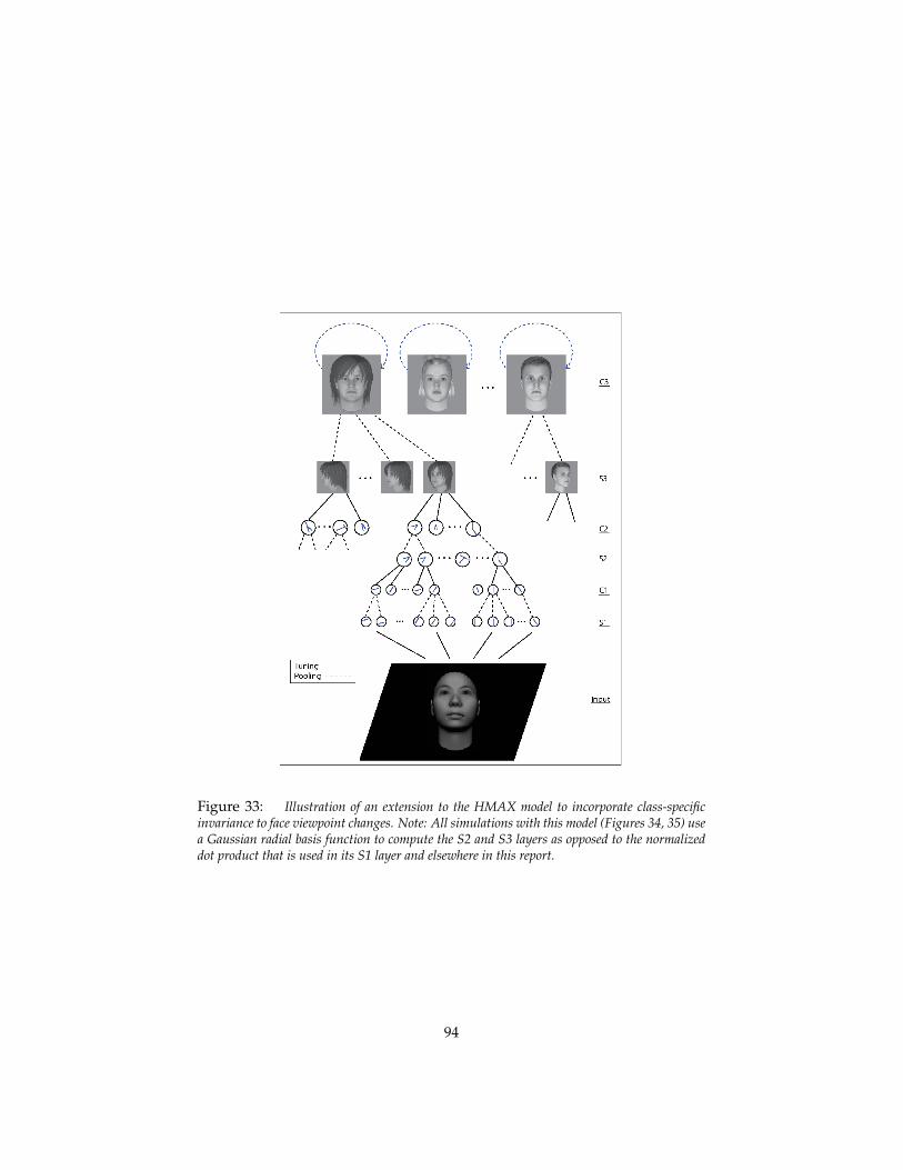
Figure 33: Illustration of an extension to the HMAX model to incorporate class-specificinvariance to face viewpoint changes. Note: All simulations with this model (Figures 34, 35) usea Gaussian radial basis function to compute the S2 and S3 layers as opposed to the normalizeddot product that is used in its S1 layer and elsewhere in this report.
94
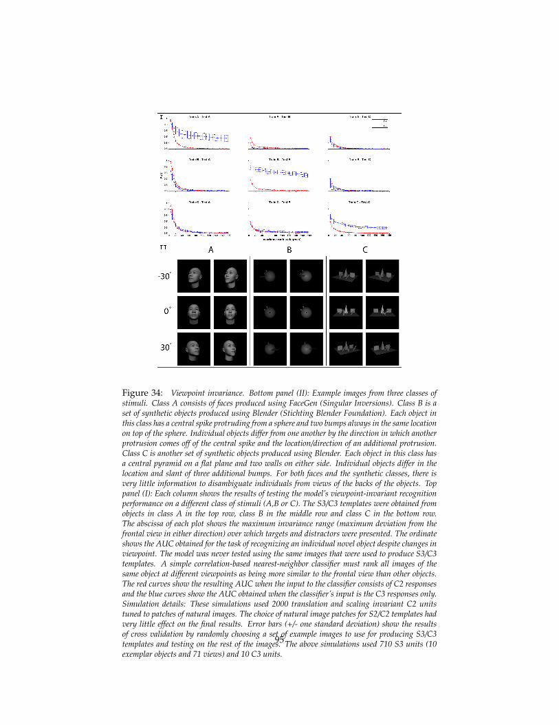
Figure 34: Viewpoint invariance. Bottom panel (II): Example images from three classes ofstimuli. Class A consists of faces produced using FaceGen (Singular Inversions). Class B is aset of synthetic objects produced using Blender (Stichting Blender Foundation). Each object inthis class has a central spike protruding from a sphere and two bumps always in the same locationon top of the sphere. Individual objects differ from one another by the direction in which anotherprotrusion comes off of the central spike and the location/direction of an additional protrusion.Class C is another set of synthetic objects produced using Blender. Each object in this class hasa central pyramid on a flat plane and two walls on either side. Individual objects differ in thelocation and slant of three additional bumps. For both faces and the synthetic classes, there isvery little information to disambiguate individuals from views of the backs of the objects. Toppanel (I): Each column shows the results of testing the model’s viewpoint-invariant recognitionperformance on a different class of stimuli (A,B or C). The S3/C3 templates were obtained fromobjects in class A in the top row, class B in the middle row and class C in the bottom row.The abscissa of each plot shows the maximum invariance range (maximum deviation from thefrontal view in either direction) over which targets and distractors were presented. The ordinateshows the AUC obtained for the task of recognizing an individual novel object despite changes inviewpoint. The model was never tested using the same images that were used to produce S3/C3templates. A simple correlation-based nearest-neighbor classifier must rank all images of thesame object at different viewpoints as being more similar to the frontal view than other objects.The red curves show the resulting AUC when the input to the classifier consists of C2 responsesand the blue curves show the AUC obtained when the classifier’s input is the C3 responses only.Simulation details: These simulations used 2000 translation and scaling invariant C2 unitstuned to patches of natural images. The choice of natural image patches for S2/C2 templates hadvery little effect on the final results. Error bars (+/- one standard deviation) show the resultsof cross validation by randomly choosing a set of example images to use for producing S3/C3templates and testing on the rest of the images. The above simulations used 710 S3 units (10exemplar objects and 71 views) and 10 C3 units.
95

Figure 35: Illumination invariance. Same organization as in figure 3. Bottom panel (II):Example images from three classes of stimuli. Each class consists of faces with different lightreflectance properties, modeling different materials. Class A was opaque and non-reflective likewood. Class B was opaque but highly reflective like a shiny metal. Class C was translucent likeglass. Each image shows a face’s appearance corresponding to a different location of the sourceof illumination (the lamp). The face models were produced using FaceGen and modified withBlender. Top panel (I): Columns show the results of testing illumination-invariant recognitionperformance on class A (left), B (middle) and C (right). S3/C3 templates were obtained from ob-jects in class A (top row), B (middle row), and C (bottom row). The model was never tested usingthe same images that were used to produce S3/C3 templates. As in figure 3, the abscissa of eachplot shows the maximum invariance range (maximum distance the light could move in eitherdirection away from a neutral position where the lamp is even with the middle of the head) overwhich targets and distractors were presented. The ordinate shows the AUC obtained for the taskof recognizing an individual novel object despite changes in illumination. A correlation-basednearest-neighbor “classifier” must rank all images of the same object under each illuminationcondition as being more similar to the neutral view than other objects. The red curves show theresulting AUC when the input to the classifier consists of C2 responses and the blue curves showthe AUC obtained when the classifier’s input is the C3 responses only. Simulation details: Thesesimulations used 80 translation and scaling invariant C2 units tuned to patches of natural im-ages. The choice of natural image patches for S2/C2 templates had very little effect on the finalresults. Error bars (+/- one standard deviation) show the results of cross validation by randomlychoosing a set of example images to use for producing S3/C3 templates and testing on the rest ofthe images. The above simulations used 1200 S3 units (80 exemplar faces and 15 illuminationconditions) and 80 C3 units.
96
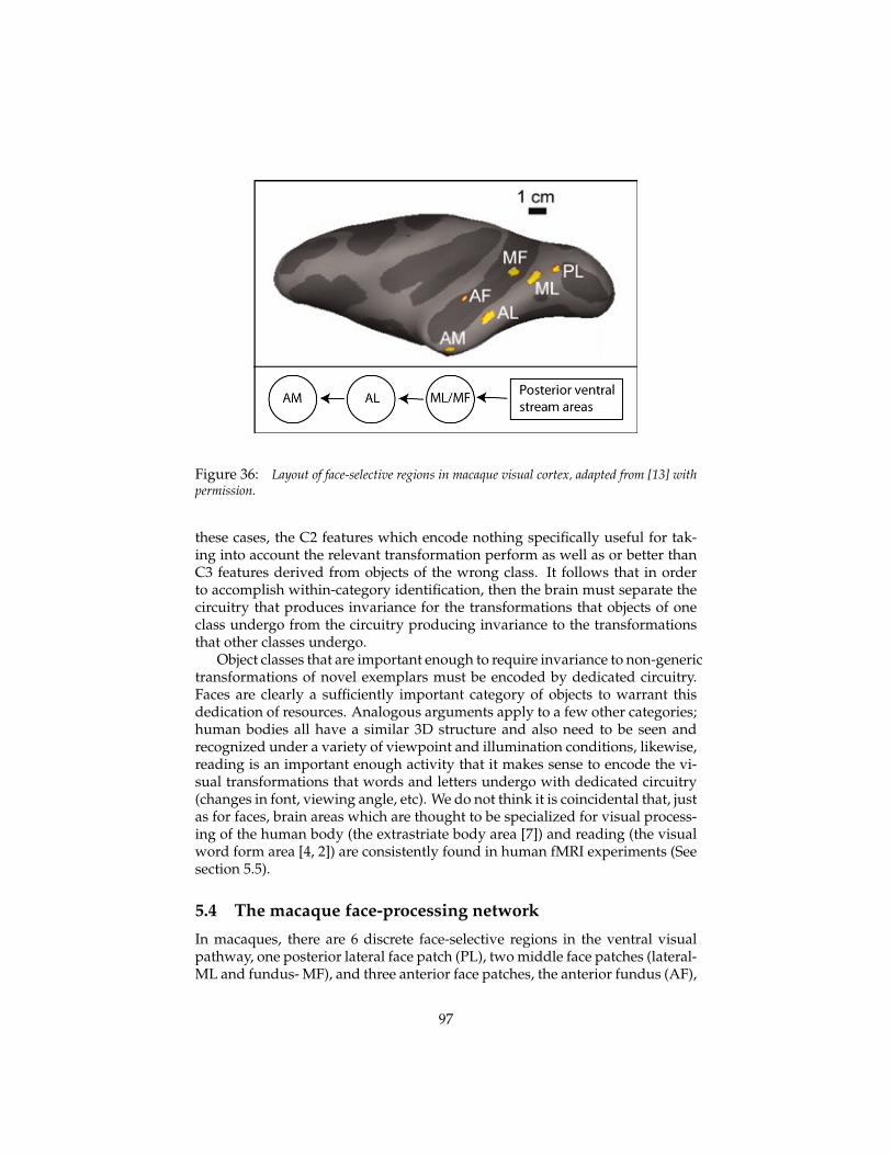
Figure 36: Layout of face-selective regions in macaque visual cortex, adapted from [13] withpermission.
these cases, the C2 features which encode nothing specifically useful for tak-ing into account the relevant transformation perform as well as or better thanC3 features derived from objects of the wrong class. It follows that in orderto accomplish within-category identification, then the brain must separate thecircuitry that produces invariance for the transformations that objects of oneclass undergo from the circuitry producing invariance to the transformationsthat other classes undergo.
Object classes that are important enough to require invariance to non-generictransformations of novel exemplars must be encoded by dedicated circuitry.Faces are clearly a sufficiently important category of objects to warrant thisdedication of resources. Analogous arguments apply to a few other categories;human bodies all have a similar 3D structure and also need to be seen andrecognized under a variety of viewpoint and illumination conditions, likewise,reading is an important enough activity that it makes sense to encode the vi-sual transformations that words and letters undergo with dedicated circuitry(changes in font, viewing angle, etc). We do not think it is coincidental that, justas for faces, brain areas which are thought to be specialized for visual process-ing of the human body (the extrastriate body area [7]) and reading (the visualword form area [4, 2]) are consistently found in human fMRI experiments (Seesection 5.5).
5.4 The macaque face-processing network
In macaques, there are 6 discrete face-selective regions in the ventral visualpathway, one posterior lateral face patch (PL), two middle face patches (lateral-ML and fundus- MF), and three anterior face patches, the anterior fundus (AF),
97

anterior lateral (AL), and anterior medial (AM) patches [71, 72]. At least someof these patches are organized into a feedforward hierarchy. Visual stimulationevokes a change in the local field potential ∼ 20 ms earlier in ML/MF than inpatch AM [13]. Consistent with a hierarchical organization involving informa-tion passing from ML/MF to AM via AL, electrical stimulation of ML eliciteda response in AL and stimulation in AL elicited a response in AM [44]. In ad-dition, spatial position invariance increases from ML/MF to AL, and increasesfurther to AM [13] as expected for a feedforward processing hierarchy.
Freiwald et al. (2010) found that the macaque face patches differ qualita-tively in how they represent identity across head orientations. Neurons in themiddle lateral (ML) and middle fundus (MF) patches were view-specific; whileneurons in the most anterior ventral stream face patch, the anterior medialpatch (AM), were view invariant. Puzzlingly, neurons in an intermediate area,the anterior lateral patch (AL), were tuned identically across mirror-symmetricviews. That is, neurons in patch AL typically have bimodal tuning curves e.g.,one might be optimally tuned to a face rotated 45 to the left and 45 to theright6 (see figure 37).
In Part II of this paper, we argued that Hebbian plasticity at the synapsesin visual cortex causes the tuning of the cells to converge to the eigenvectors oftheir input’s covariance. In this section we demonstrate that the same theory,when applied to class-specific layers, yields cells with properties that closelyresemble those of the cells in the macaque face-processing network.
5.4.1 Principal components and mirror-symmetric tuning curves
Define τ∗n,i as the i-th principal component (PC) of the templatebook obtainedfrom a single base template. For the following, assume that the templatebookT is centered (we subtract its mean as a preprocessing step). The τ∗n,i are bydefinition the eigenvectors of TᵀT: τ∗n,1 is the first PC acquired from the n-thbase pattern’s transformation, τ∗n,2 the second PC, and so on.
A frontal view of a face is symmetric about its vertical midline. Thus equalrotations in depth (e.g., 45 to the left and 45 to the right) produce images thatare reflections of one another. Therefore, the templatebook T obtained from aface’s 3D rotation in depth must have a special structure. For simplicity, con-sider only “symmetric transformation sequences”, e.g., all the neural frames ofthe rotation from a left 90 profile to a right 90 profile. For each neural frameτn,t there must be a corresponding reflected frame in the templatebook that wewill indicate as τn,−t. It will turn out that as a consequence of its having thisstructure, the eigenfunctions of the templatebook will be even and odd. There-fore, the templates obtained from compressing the templatebook as thoughthey were neural frames, are symmetric or anti-symmetric images (see figure
6Freiwald and Tsao (2010) found that 92 of the 215 AL cells in their study responded at leasttwice as strongly to one of the two full-profiles as to frontal faces. These profile-selective cellsresponded very similarly to both profiles. A subsequent test using face stimuli at more orienta-tions found that 43 of 57 cells had view tuning maps with two discrete peaks at mirror symmetricpositions.
98

Figure 37: Figure from [13]. Tuning of AL cells to a head randomly rotated in three di-mensions. (A) Illustration of stimulus head and three axes of rotation. (B) View tuning infour typical cells. Tuning to up-down angle versus left-right angle (responses averaged acrosspicture-plane angle). (Middle) Tuning to up-down angle versus picture-plane angle (responsesaveraged across left-right angle). (Bottom) Tuning to picture-plane angle versus left-right angle(responses averaged across up-down angle). Marginal tuning curves are also shown (verticallines indicate tuning peak position).
99

40).LetR denote the reflection operatorR(τn,t) = τn,−t. For simplicity, consider
a templatebook that only contains one template τ and its reflection Rτ .Let J denote the operator that takes a neural frame τ and returns the tem-
platebook consisting of τ and its reflection.
J = (I,R) (44)
J(τ) = T =(τRτ
)(45)
(46)
Thus
[JᵀJ ](Rτ) =(Rτ + ττ +Rτ
)= R([JᵀJ ](τ)) (47)
Therefore R(JᵀJ) = (JᵀJ)R, (they commute). Thus JᵀJ and R must havethe same eigenfunctions. Since the eigenfunctions of R are even or odd func-tions, the principal components of TᵀT must also be even and odd. Therefore,since we use the absolute value of the normalized dot product of the inputwith a template, both even and odd templates yield tuning curves that showidentical tuning to symmetric face views.
5.4.2 Models of the macaque face recognition hierarchy
We have shown that models of the ventral stream that compute a signature rel-ative to the principal components of the templatebooks acquired from rotationof template faces must contain an intermediate step with identical tuning tosymmetric face faces. We propose to identify patch AL with the the projectiononto principal components and patch AM with the subsequent pooling stage.
These considerations alone do not completely constrain a model of the ven-tral stream. In order to demonstrate the working of these models and performvirtual electrophysiology experiments to test the properties of the simulatedcells, we must make some other parameter and architectural choices. We inves-tigated several model architectures. Each one corresponds to different choiceswe made about the processing of the visual signal prior to face patch AL (seefigure 38).
At run time, cells in the S-PCA layer compute the absolute value of thenormalized dot product of their stored PC with the input. Each cell in the C-PCA layer pools over all the cells in the S-PCA layer with PCs from the sametemplatebook.
In the developmental phase, the S-PCA templates are acquired by PCA ofthe templatebooks. Each templatebook contains all the (vectorized) images ofthe rotation (in depth) of a single face. All the 3D models used to producetraining and testing images were produced by FaceGen7 and rendered with
7Singular Inversions Inc.
100
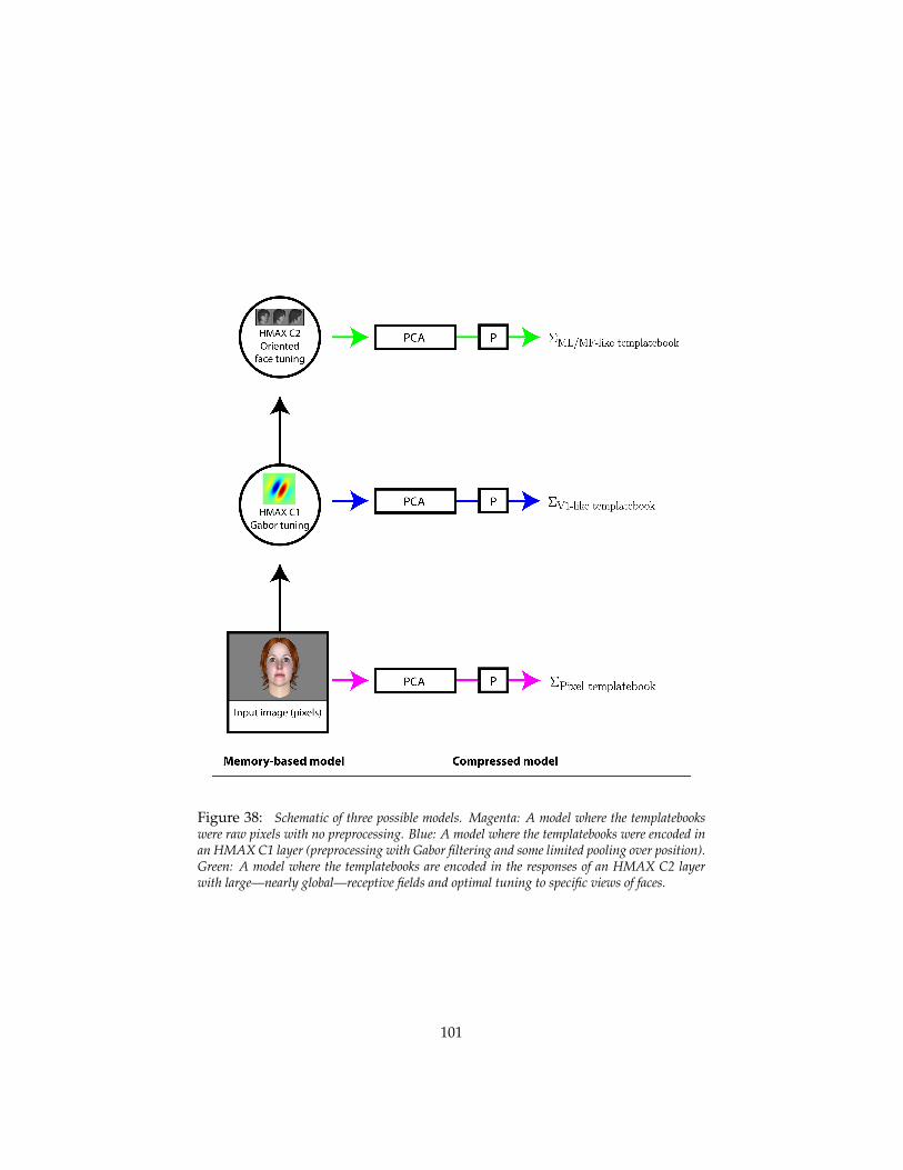
Figure 38: Schematic of three possible models. Magenta: A model where the templatebookswere raw pixels with no preprocessing. Blue: A model where the templatebooks were encoded inan HMAX C1 layer (preprocessing with Gabor filtering and some limited pooling over position).Green: A model where the templatebooks are encoded in the responses of an HMAX C2 layerwith large—nearly global—receptive fields and optimal tuning to specific views of faces.
101
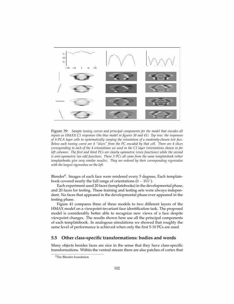
Figure 39: Sample tuning curves and principal components for the model that encodes allinputs as HMAX C1 responses (the blue model in figures 38 and 41). Top row: the responsesof S-PCA layer cells to systematically varying the orientation of a randomly-chosen test face.Below each tuning curve are 4 “slices” from the PC encoded by that cell. There are 4 slicescorresponding to each of the 4 orientations we used in the C1 layer (orientations shown in farleft column). The first and third PCs are clearly symmetric (even functions) while the secondis anti-symmetric (an odd function). These 3 PCs all came from the same templatebook (othertemplatebooks give very similar results). They are ordered by their corresponding eigenvaluewith the largest eigenvalue on the left.
Blender8. Images of each face were rendered every 5 degrees, Each template-book covered nearly the full range of orientations (0− 355).
Each experiment used 20 faces (templatebooks) in the developmental phase,and 20 faces for testing. These training and testing sets were always indepen-dent. No faces that appeared in the developmental phase ever appeared in thetesting phase.
Figure 41 compares three of these models to two different layers of theHMAX model on a viewpoint-invariant face identification task. The proposedmodel is considerably better able to recognize new views of a face despiteviewpoint changes. The results shown here use all the principal componentsof each templatebook. In analogous simulations we showed that roughly thesame level of performance is achieved when only the first 5-10 PCs are used.
5.5 Other class-specific transformations: bodies and words
Many objects besides faces are nice in the sense that they have class-specifictransformations. Within the ventral stream there are also patches of cortex that
8The Blender foundation
102
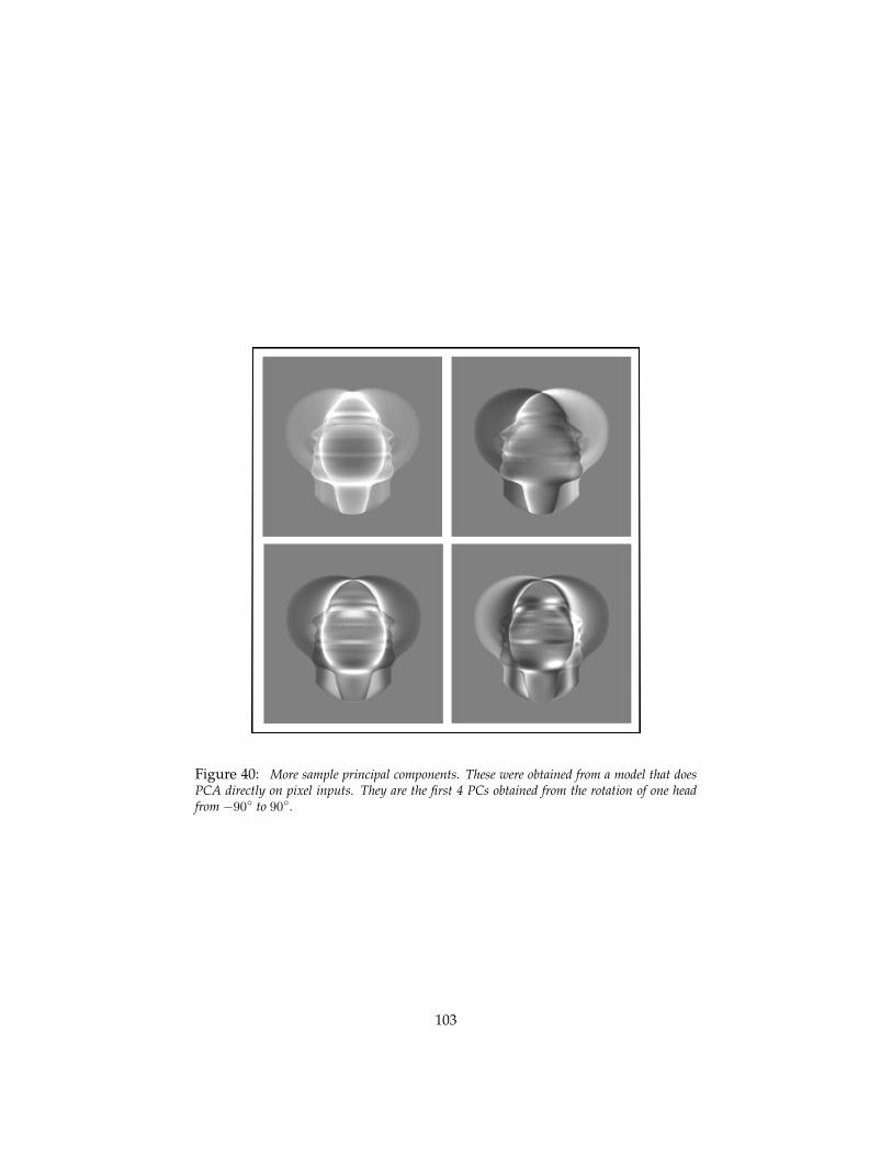
Figure 40: More sample principal components. These were obtained from a model that doesPCA directly on pixel inputs. They are the first 4 PCs obtained from the rotation of one headfrom −90 to 90.
103
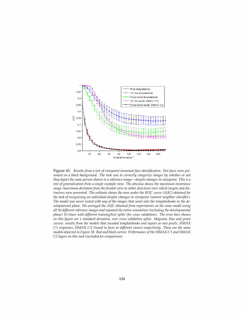
Figure 41: Results from a test of viewpoint-invariant face identification. Test faces were pre-sented on a black background. The task was to correctly categorize images by whether or notthey depict the same person shown in a reference image—despite changes in viewpoint. This is atest of generalization from a single example view. The abscissa shows the maximum invariancerange (maximum deviation from the frontal view in either direction) over which targets and dis-tractors were presented. The ordinate shows the area under the ROC curve (AUC) obtained forthe task of recognizing an individual despite changes in viewpoint (nearest neighbor classifier).The model was never tested with any of the images that went into the templatebooks in the de-velopmental phase. We averaged the AUC obtained from experiments on the same model usingall 20 different reference images and repeated the entire simulation (including the developmentalphase) 10 times with different training/test splits (for cross validation). The error bars shownon this figure are 1 standard deviation, over cross validation splits. Magenta, blue and greencurves: results from the models that encoded templatebooks and inputs as raw pixels, HMAXC1 responses, HMAX C2 (tuned to faces at different views) respectively. These are the samemodels depicted in Figure 38. Red and black curves: Performance of the HMAXC1 and HMAXC2 layers on this task (included for comparison).
104

Figure 42: Left: Images of human bodies in various poses were used to train and test themodel. 1280 3D object models of human body were created with DAZ 3D Studio and one256*256 pixel greyscale image was rendered from each object automatically with blender. The1280 objects consisted of 40 differently shaped human bodies in 32 poses. The 40 bodies wereeither male or female, had varying degrees of fatness, muscularity, and limb proportion. The32 poses were natural, commonly encountered poses such as waving, running, leaning, andclinging. Right: Performance of class-specific models and HMAX control models on a pose-invariant body recognition task. 10 bodies were used for testing. The abscissa is the number ofbodies used to train the model. Performance was averaged over 10 cross-validation runs. Theerror bars correspond to standard deviations of AUC values over the cross-validation runs.
show BOLD responses for non-face objects. These include regions that respondto scenes—the parahippocampal place area (PPA) [8]—written words—the vi-sual word form area (VWFA) [4], and bodies—the extrastriate body area (EBA)and the fusiform body area (FBA) [7, 50]. Many of these regions were shownto be necessary for recognition tasks with the objects they process by lesionstudies ([34, 45]) and TMS ([75, 52]. We have begun to study transformationsof two of these: bodies (different poses, actions) and printed words (changesin font, viewing angle, etc.) (See also the preliminary report of our work onscenes: [27]).
Figures 42 and 43 show the results of class-specific invariant recognitiontasks for bodies—identification of a specific body invariantly to its pose—andwords—font-invariant word recognition. In both cases, the models that em-ploy class-specific features (they pooling over templates depicting differentbodies or different fonts) outperform control HMAX models. Additional de-tails on these models will soon be available in forthcoming reports from ourgroup.
Remark: Throughout this report we have held temporal contiguity to be
105

Figure 43: Words (4-grams) were chosen from a fixed alphabet of 4 letters. A nearest-neighborclassifier ranked each image—of a word in a particular font—by its similarity to the image ofa reference word. Templatebooks were obtained from translated and font-transformed imagesof single letters, bigrams and trigrams. Red, blue and green curves: These used a version ofthe compression-based model described in part II of this report. Black curve: An HMAX C2model with global pooling (for comparison). The S2 dictionary consisted of 2000 patches ofnatural images. The abscissa is the number of partial words (bigrams and trigrams) used inthe templatebook. Error bars are +/- 1 standard deviation, over 5 runs of the simulation usingdifferent randomly chosen bigrams, trigrams and testing words. This simulation used 4 differentfonts.
106

an important cue for associating the frames of the video of an object’s trans-formation with one another. That approach cannot be taken to learn thesebody/word recognition models. The former model requires the associationof different bodies under the same pose and the latter requires the same words(rather: partial words) to be associated under a variety of fonts. A temporal-contiguity based learning rule could not be used to learn the pooling domainsfor these tasks. Additionally, in other sensory modalities (such as audition) rec-ognizing temporally extended events is common. It is not clear how temporalcontiguity-based arguments could apply in those situations.
5.6 Invariance to X and estimation of X
So far we have discussed the problem of recognition as estimating identityor category invariantly to a transformation X – such as translation or pose orillumination. Often however, the key problem is the complementary one, ofestimating X, for instance pose, possibly independently of identity. The sameneural population may be able to support both computations as shown in ITrecordings [22] and model simulations [64]. We are certainly able to estimateposition, rotation, illumination of an object without eye movements, thoughprobably not very precisely. In the ventral stream this may require the use oflower-level signatures, possibly in a task-dependent way. This may involveattention.
Figure 44 shows the results on the task of recognizing the pose—out of aset of 32 possibilities—of a body invariantly to which body is shown. Noticethat low-level visual features (HMAX C1) work just as well on this task as theclass-specific features.
107
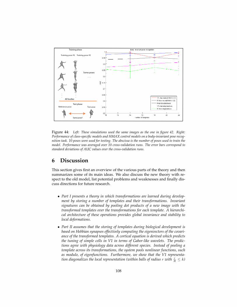
Figure 44: Left: These simulations used the same images as the one in figure 42. Right:Performance of class-specific models and HMAX control models on a body-invariant pose recog-nition task. 10 poses were used for testing. The abscissa is the number of poses used to train themodel. Performance was averaged over 10 cross-validation runs. The error bars correspond tostandard deviations of AUC values over the cross-validation runs.
6 Discussion
This section gives first an overview of the various parts of the theory and thensummarizes some of its main ideas. We also discuss the new theory with re-spect to the old model, list potential problems and weaknesses and finally dis-cuss directions for future research.
• Part I presents a theory in which transformations are learned during develop-ment by storing a number of templates and their transformations. Invariantsignatures can be obtained by pooling dot products of a new image with thetransformed templates over the transformations for each template. A hierarchi-cal architecture of these operations provides global invariance and stability tolocal deformations.
• Part II assumes that the storing of templates during biological development isbased on Hebbian synapses effectively computing the eigenvectors of the covari-ance of the transformed templates. A cortical equation is derived which predictsthe tuning of simple cells in V1 in terms of Gabor-like wavelets. The predic-tions agree with physiology data across different species. Instead of pooling atemplate across its transformations, the system pools nonlinear functions, suchas modulo, of eigenfunctions. Furthermore, we show that the V1 representa-tion diagonalizes the local representation (within balls of radius r with r
R ≤ k)
108

of similitude transformations of the image as independent shifts in a 4D space.Thus learning at higher layers generates 4D wavelets. The prediction may beconsistent with physiology data
• Part III shows that non-affine transformations on the image plane (such as theimage changes induced by 3D rotations of an object) can be well approximatedby the template and dot-product module described in Part I and II for certain ob-ject classes, provided that the transformed templates capture class-specific trans-formation. The theory explains several properties of faces patches in macaquecortex. It also suggests how pooling over transformations can provide identity-specific, pose-invariant representations whereas pooling over identities (tem-plates) provides pose-specific, identity-invariant representations.
6.1 Some of the main ideas
There are several key ideas in the theoretical framework of the paper. We re-count here ideas already mentioned in the paper.
1. We conjecture that the sample complexity of object recognition is mostlydue to geometric image transformations (e.g. different viewpoints) andthat a main goal of the ventral stream – V1, V2, V4 and IT – is to learn-and-discount image transformations.
2. The most surprising implication of the theory emerging from these spe-cific assumptions is that the computational goals and detailed propertiesof cells in the ventral stream follow from symmetry properties of the visualworld through a process of correlational learning. The obvious analogyis physics: for instance, the main equation of classical mechanics can bederived from general invariance principles. In fact one may argue thata Foldiak-type rule together with the physics of the world is all that isneeded by evolution to determine through developmental learning thehierarchical organization of the ventral stream, the transformations thatare learned and the tuning of the receptive fields in each visual area.
3. Aggregation functions such as the modulo square or approximations ofit or the max (as in HMAX or in [30]) ensure that signatures of images areinvariant to affine transformations of the image and that this property ispreserved from layer to layer.
4. The theory assumes that there is a hierarchical organization of areas of theventral stream with increasingly larger receptive apertures of increasingsize determining a stratification of the range of invariances. At the small-est size there are effectively only translations.
5. Another idea is that memory-based invariances determine the spectralproperties of samples of transformed images and thus of a set of tem-plates recorded by a memory-based recognition architecture such as an(extended) HMAX.
109

6. Spectral properties of the input determine receptive field tuning via Hebbian-like online learning rules that converge to the principal components ofthe inputs.
7. Signatures from all layers access the associative memory or classifier mod-ule and thus control iterations in visual recognition and processing. Ofcourse, at lower layers there are many signatures, each one in differentcomplex cell layer locations, while at the top layer there are only a smallnumber of signatures – in the limit only one.
The theory of this paper starts with this central computational problem inobject recognition: identifying or categorizing an object after looking at a sin-gle example of it – or of an exemplar of its class. To paraphrase Stu Geman,the difficulty in understanding how biological organisms learn – in this casehow they recognize – is not the usual n → ∞ but n → 0. The mathematicalframework is inspired by known properties of neurons and visual cortex anddeals with the problem of how to learn and discount invariances. Motivatedby the Johnson-Lindenstrauss theorem, we introduce the notion of a signatureof an object as a set of similarity measurements with respect to a small set oftemplate images. An invariance lemma shows that the stored transformationsof the templates allow the retrieval of an invariant signature of an object forany uniform transformation of it such as an affine transformation in 2D. Sinceany transformation of an image can be approximated by local affine transfor-mations, corresponding to a set of local receptive fields, the invariance lemmaprovides a solution for the problem of recognizing an object after experiencewith a single image – under conditions that are idealized but hopefully cap-ture a good approximation of reality. Memory-based hierarchical architecturesare much better at learning transformations than non-hierarchical architecturesin terms of memory requirements. This part of the theory shows how the hi-erarchical architecture of the ventral stream with receptive fields of increasingsize (roughly by a factor of 2 from V1 to V2 and again from V2 to V4 and fromV4 to IT) could implicitly learn during development different types of transfor-mations starting with local translations in V1 to a mix of translations and scalesand rotations in V2 and V4 up to more global transformations in PIT and AIT(the stratification conjecture).
Section 4 speculates on how the properties of the specific areas may be de-termined by visual experience and continuous plasticity and characterizes thespectral structure of the templatebooks arising from various types of transfor-mations that can be learned from images. A conjecture – to be verified withsimulations and other empirical studies – is that in such an architecture theproperties of the receptive fields in each area are mostly determined by theunderlying transformations rather than the statistics of natural images. Thelast section puts together the previous results into a detailed hypothesis of theplasticity, the circuits and the biophysical mechanisms that may subserve thecomputations in the ventral stream.
In summary, some of the broad predictions of this theory-in-fieri are:
110

• each cell’s tuning properties are shaped by visual experience of imagetransformations during developmental and adult plasticity;
• the mix of transformations – seen from the retina – learned in each areainfluences the tuning properties of the cells – oriented bars in V1+V2,radial and spiral patterns in V4 up to class specific tuning in AIT (e.g.face tuned cells);
• during evolution, areas above V1 should appear later than V1, reflect-ing increasing object categorization abilities and the need for invariancesbeyond translation;
• an architecture based on signatures that are invariant (from an area atsome level) to affine transformations may underly perceptual constancyagainst small eye movements and other small motions9.
• invariance to affine transformations (and others) can provide the seed forevolutionary development of “conceptual” invariances;
• the transfer of invariance accomplished by the machinery of the template-books may be used to implement high level abstractions;
• the preceding sections stressed that the statistics of natural images donot play a primary role in determining the spectral properties of the tem-platebook and, via the linking theorem the tuning of the cells in specificareas. This is usually true for the early areas under normal developmentconditions. It is certainly not true if development takes place in a de-prived situation. The equations show that the spectrum of the imagesaveraged over the presentations affects the spectral content, e.g. the cor-relation matrix and thus the stationary solutions of Hebbian learning.
• In summary, from the assumption of a hierarchy of areas with receptivefields of increasing size the theory predicts that the size of the recep-tive fields determines which transformations are learned during devel-opment and then factored out during normal processing; that the trans-formation represented in an area determines the tuning of the neuronsin the area; and that class-specific transformations are learned and repre-sented at the top of the hierarchy.
6.2 Extended model and previous model
So far in this paper, existing hierarchical models of visual cortex – eg HMAX –are reinterpreted and extended in terms of computational architectures whichevolved to discount image transformations learned from experience. From thisnew perspective, I argue that a main goal of cortex is to learn equivalence
9There may be physiological evidence (from Motter and Poggio) suggesting invariance of sev-eral minutes of arc at the level of V1 and above.
111

classes consisting of patches of images (that we call templates), associated to-gether since they are observed in close temporal contiguity – in fact as a tempo-ral sequence – and are therefore likely to represent physical transformations ofthe same object (or part of the same object). I also conjecture that the hierarchy –and the number of layers in it - is then determined by the need to learn a groupof transformations – such as the affine group. I prove that a simple memory-based architecture can learn invariances from the visual environment and canprovide invariant codes to higher memory areas. I also discuss the possibil-ity that the size of the receptive fields determines the type of transformationswhich are learned by different areas of cortex from the natural visual world– from local translations to local rotations and image-plane affine transforma-tions up to almost global translations and viewpoint/pose/expression trans-formations. Earlier layers would mostly represent local generic transforma-tions such as translation and scale and other similitude transformations. Sim-ilar considerations imply that the highest layers may represent class-specifictransformations such as rotations in depth of faces or changes in pose of bod-ies.
• The present HMAX model has been hardwired to deal with 2 generictransformations: translation and scale. The model performance on ”pure”translation tasks is perfect (apart from discretization noise), while it de-clines quickly with viewpoint changes (±20 degrees is roughly the in-variance range).
• As mentioned several times, the theory assumes that signatures fromseveral layers can be used by the associative memory- classifier at thetop, possibly under attentional or top-down control, perhaps via cortical-pulvinar-cortical connections.
• What matters for recognition is not the strong response of a populationof neurons (representing a signature) but the invariance of the responsein order to provide a signal, invariant as possible, to the classifier.
• Untangling invariance Getting invariance is easy if many examples of thespecific object are available. What is difficult is getting invariance froma single example of an object (or very few). Many of the discussions ofinvariance are confused by failing to recognize this fact. Untangling in-variance is easy10 when a sufficiently large number of previously seenviews of the object are available, by using smooth nonlinear interpola-tion techniques such as RBFs.
6.3 What is under the carpet
Here is a list of potential weaknesses, small and large, with some comments:
10apart from self-occlusions and uniqueness problems. Orthographic projections in 2D of thegroup Aff(3,R) are not a group; however the orthographic projections of translations in x, y, zand rotations in the image plane are a group.
112

• “The theory is too nice to be true”. One of the main problems of thetheory is that it seems much too elegant – in the sense of physics – forbiology.
• Backprojections are not taken into account and they are a very obviousfeature of the anatomy, which any real theory should explain. Backpro-jections and top-down controls are however implied by the present the-ory. The most obvious limitation of feedforward architectures is recog-nition in clutter and the most obvious way around the problem is theattentional masking of large parts of the image under top-down con-trol. More in general, a realistic implementation of the present theoryrequires top-down control signals and circuits, supervising learning andpossibly fetching signatures from different areas and at different loca-tions in a task-dependent way. An even more interesting hypothesis isthat backprojections update local signatures at lower levels depending onthe scene class currently detected at the top (an operation similar to thetop-down pass of Ullman). In summary, the output of the feedforwardpass is used to retrieve labels and routines associated with the image;backprojections implement an attentional focus of processing to reduceclutter effects and also run spatial visual routines at various levels of thehierarchy.
• Subcortical projections, such as, for instance, projections to and from thepulvinar, are not predicted by the theory. The present theory still is (un-fortunately) in the “cortical chauvinism” camp. Hopefully somebodywill rescue it.
• Cortical areas are organized in a series of layers with specific types of cellsand corresponding arborizations and connectivities. The theory does notsay anything at this point about this level of the circuitry.
6.4 Directions for future research
6.4.1 Associative memories
In past work on HMAX we assumed that the hierarchical architecture performsa kind of preprocessing of an image to provide, as result of the computation,a vector (that we called “signature” here) that is then input to a classifier. Thisview is extended in this paper by assuming that the signature vector is input toan associative memory so that a number of properties of the image (and asso-ciations) can be recalled. Parenthetically we note that old associative memoriescan be regarded as vector-valued classifiers – an obvious observation.
Retrieving from an associative memory: optimal sparse encoding and recall Thereare interesting estimates of optimal properties of codes for associative mem-ories, including optimal sparsness (see [49, 54]). It would be interesting toconnect these results to estimated capacity of visual memory (Oliva, 2010).
113

Weak labeling by association of video frames Assume that the top associativemodule associates together images in a video that are contiguous in time (apartwhen there are clear transitions). This idea (mentioned to TP by Kai Yu) relieson smoothness in time to label via association. It is a very biological semi-supervised learning, very much in tune with our proposal of the S:C memory-based module for learning invariances to transformations and with the ideasabove about an associative memory module at the very top.
Space, time, scale, orientation Space and time are in a sense intrinsic to imagesand to their measurement. It seems that the retina is mainly dealing with thosethree dimensions (x, y, t), though x, y are sampled according to the samplingtheorem in a way which is eccentricity-dependent forcing in later cortical layersthe development of receptive field with a size which increases with eccentricity(spacing in the lattice and scale of receptive fields increase proportionally to∼ logr).
The theory assumes that at each eccentricity a set of receptive fields of dif-ferent size (eg σ) exist during development at the level of developing simplecells, originating a set of scales. It is an open question what drove evolution todiscover multiresolution analysis of the image. Given finite channel resources– eg bandwidth, number of fibers, number of bits – there is a tradeoff betweensize of the visual field and scale (defined as the resolution in terms of spa-tial frequency cutoff). Once multiple scales are superimposed on space (eg alattice of ganglion cells in each x, y) by a developmental program, our theorydescribes how the orientation dimension is necessarily discovered by exposureto moving images.
6.4.2 Visual abstractions
• Concept of parallel lines Consider an architecture using signatures. Assumeit has learned sets of templates that guarantee invariance to all affinetransformations. The claim is that the architecture will abstract the concept ofparallel lines from a single specific example of two parallel lines. The argumentis that according to the theorems in the paper, the signature of the singleimage of the parallel lines will be invariant to any affine transformations.
• Number of items in an image A classifier which learns the number five ina way which is invariant to scale should be able to recognize five objectsindependent of class of objects.
• Line drawings conjecture The memory-based module described in this pa-per should be able to generalize from real images to line drawings whenexposed to illumination-dependent transformations of images. This mayneed to happen at more than one level in the system, starting with thevery first layer (eg V1). Generalizations with respect to recognition ofobjects invariant to shadows may also be possible.
114
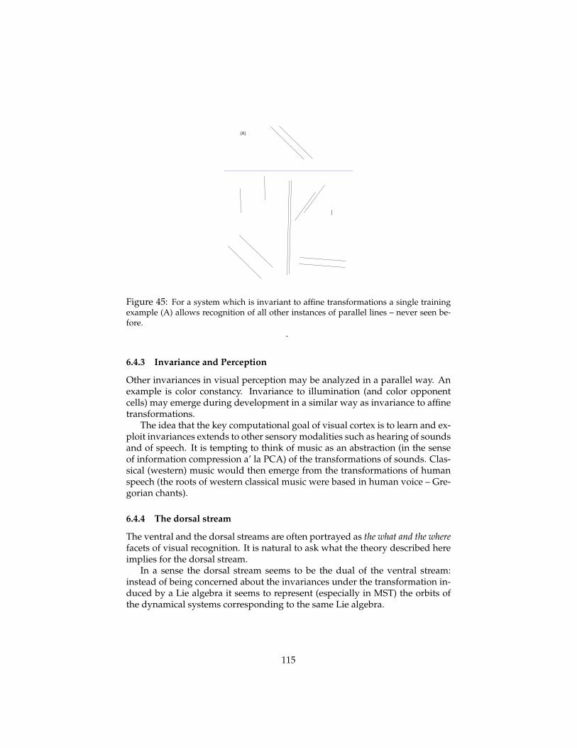
(A)
Figure 45: For a system which is invariant to affine transformations a single trainingexample (A) allows recognition of all other instances of parallel lines – never seen be-fore.
.
6.4.3 Invariance and Perception
Other invariances in visual perception may be analyzed in a parallel way. Anexample is color constancy. Invariance to illumination (and color opponentcells) may emerge during development in a similar way as invariance to affinetransformations.
The idea that the key computational goal of visual cortex is to learn and ex-ploit invariances extends to other sensory modalities such as hearing of soundsand of speech. It is tempting to think of music as an abstraction (in the senseof information compression a’ la PCA) of the transformations of sounds. Clas-sical (western) music would then emerge from the transformations of humanspeech (the roots of western classical music were based in human voice – Gre-gorian chants).
6.4.4 The dorsal stream
The ventral and the dorsal streams are often portrayed as the what and the wherefacets of visual recognition. It is natural to ask what the theory described hereimplies for the dorsal stream.
In a sense the dorsal stream seems to be the dual of the ventral stream:instead of being concerned about the invariances under the transformation in-duced by a Lie algebra it seems to represent (especially in MST) the orbits ofthe dynamical systems corresponding to the same Lie algebra.
115

6.4.5 Is the ventral stream a cortical mirror of the invariances of the physicalworld?
It is somewhat intriguing that Gabor frames - related to the “coherent” statesand the squeezed states of quantum mechanics - emerge from the filtering op-erations of the retina which are themselves a mirror image of the position andmomentum operator in a Gaussian potential. It is even more intriguing that in-variances to the group SO2×R2 dictate, according to our theory, the computa-tional goals, the hierarchical organization and the tuning properties of neuronsin visual areas. In other words: it did not escape our attention that the theorydescribed here implies that the brain function, structure and properties reflectin a surprising direct way the physics of the visual world.
Acknowledgments We would like to especially thank Steve Smale, Leyla Isik,Owen Lewis, Steve Voinea, Alan Yuille, Stephane Mallat, Mahadevan, S. Ullman fordiscussions leading to this preprint and S. Soatto, J. Cowan, W. Freiwald, D. Tsao, A.Shashua, L. Wolf for reading versions of it. Andreas Maurer contributed the argu-ment about small apertures in section 4.1.1. Giacomo Spigler, Heejung Kim, and Dar-rel Deo contributed several results including simulations. Krista Ehinger and AudeOliva provided to J.L. the images of Figure 3 and we are grateful to them to makethem available prior to publication. In recent years many collaborators contributedindirectly but considerably to the ideas described here: S. Ullman, H. Jhuang, C. Tan,N. Edelman, E. Meyers, B. Desimone, T. Serre, S. Chikkerur, A. Wibisono, J. Bouvrie,M. Kouh, M. Riesenhuber, J. DiCarlo, E. Miller, A. Oliva, C. Koch, A. Caponnetto, C.Cadieu, U. Knoblich, T. Masquelier, S. Bileschi, L. Wolf, E. Connor, D. Ferster, I. Lampl,S. Chikkerur, G. Kreiman, N. Logothetis. This report describes research done at theCenter for Biological and Computational Learning, which is in the McGovern Institutefor Brain Research at MIT, as well as in the Dept. of Brain and Cognitive Sciences,and which is affiliated with the Computer Sciences and Artificial Intelligence Labora-tory (CSAIL). This research was sponsored by grants from DARPA (IPTO and DSO),National Science Foundation (NSF-0640097, NSF-0827427), AFSOR-THRL (FA8650-05-C-7262). Additional support was provided by: Adobe, Honda Research Institute USA,King Abdullah University Science and Technology grant to B. DeVore, NEC, Sony andespecially by the Eugene McDermott Foundation.
116
References[1] J. Antoine, R. Murenzi, P. Vandergheynst, and S. Ali. Two-dimensional wavelets and
their relatives. Cambridge University Press, Cambridge, UK, 2004.[2] C. Baker, J. Liu, L. Wald, K. Kwong, T. Benner, and N. Kanwisher. Visual word
processing and experiential origins of functional selectivity in human extrastriatecortex. Proceedings of the National Academy of Sciences, 104(21):9087, 2007.
[3] Y. Bengio and Y. LeCun. Scaling learning algorithms towards ai. Large-Scale KernelMachines, 34, 2007.
[4] L. Cohen, S. Dehaene, and L. Naccache. The visual word form area. Brain,123(2):291, 2000.
[5] D. Cox, P. Meier, N. Oertelt, and J. DiCarlo. ’Breaking’position-invariant objectrecognition. Nature Neuroscience, 8(9):1145–1147, 2005.
[6] Y. Dan, A. J. J., and R. C. Reid. Effcient Coding of Natural Scenes in the LateralGeniculate Nucleus: Experimental Test of a Computational Theory. The Journal ofNeuroscience, (16):3351 – 3362, 1996.
[7] P. Downing and Y. Jiang. A cortical area selective for visual processing of thehuman body. Science, 293(5539):2470, 2001.
[8] R. Epstein and N. Kanwisher. A cortical representation of the local visual environ-ment. Nature, 392(6676):598–601, 1998.
[9] M. Ferraro and T. M. Caelli. Relationship between integral transform invariancesand lie group theory. J. Opt. Soc. Am. A, 5(5):738–742, 1988.
[10] P. Foldiak. Learning invariance from transformation sequences. Neural Computa-tion, 3(2):194–200, 1991.
[11] M. Franzius, N. Wilbert, and L. Wiskott. Invariant object recognition and poseestimation with slow feature analysis. Neural Computation, 23(9):2289–2323, 2011.
[12] J. Freeman and E. Simoncelli. Metamers of the ventral stream. Nature Neuroscience,14:11951201, 2011.
[13] W. Freiwald and D. Tsao. Functional Compartmentalization and Viewpoint Gen-eralization Within the Macaque Face-Processing System. Science, 330(6005):845,2010.
[14] J. Gallant, J. Braun, and D. V. Essen. Selectivity for polar, hyperbolic, and Cartesiangratings in macaque visual cortex. Science, 1993.
[15] L. Galli and L. Maffei. Spontaneous impulse activity of rat retinal ganglion cells inprenatal life. Science (New York, NY), 242(4875):90, 1988.
[16] L. Glass and R. Perez. Perception of Random Dot Interference Patterns. Nature,31(246):360–362, 1973.
[17] K. Groechenig. Multivariate gabor frames and sampling of entire functions of sev-eral variables. Appl. Comp. Harm. Anal., pages 218 – 227, 2011.
[18] A. Grossman, J. Morlet, and T. Paul. Transforms associated to square integrablegroup representations. ii: Examples. In Annales de l’IHP Physique theorique, vol-ume 45, pages 293–309. Elsevier, 1986.
[19] J. Hegde and D. Van Essen. Selectivity for complex shapes in primate visual areaV2. Journal of Neuroscience, 20(5):61, 2000.
[20] G. Hinton and R. Memisevic. Learning to represent spatial transformations withfactored higher-order boltzmann machines. Neural Computation, 22:14731492, 2010.
[21] W. Hoffman. The Lie algebra of visual perception. Journal of Mathematical Psychol-ogy, 3(1):65–98, 1966.
117

[22] C. P. Hung, G. Kreiman, T. Poggio, and J. J. DiCarlo. Fast Readout of Object Identityfrom Macaque Inferior Temporal Cortex. Science, 310(5749):863–866, Nov. 2005.
[23] A. Hyvrinen and E. Oja. Independent component analysis: algorithms and appli-cations. Neural Networks, 13:411–430, 2000.
[24] L. Isik, J. Z. Leibo, and T. Poggio. Learning and disrupting invariance in visualrecognition with a temporal association rule. Frontiers in Computational Neuro-science, 6, 2012.
[25] J. P. Jones and L. A. Palmer. An evaluation of the two-dimensional Gabor filtermodel of simple receptive fields in cat striate cortex. Journal of Neurophysiology,58(6):1233–1258, 1987.
[26] J. Karhunen. Stability of Oja’s PCA subspace rule. Neural Comput., 6:739–747, July1994.
[27] E. Y. Ko, J. Z. Leibo, and T. Poggio. A hierarchical model of perspective-invariant scene identification. In Society for Neuroscience Annual Meeting Abstracts(486.16/OO26), Washington DC, USA, 2011.
[28] J. Koenderink. The brain a geometry engine. Psychological Research, 52(2):122–127,1990.
[29] M. Kouh and T. Poggio. A canonical neural circuit for cortical nonlinear operations.Neural computation, 20(6):1427–1451, 2008.
[30] A. Krizhevsky, I. Sutskever, and G. Hinton. Imagenet classification with deep con-volutional neural networks. Advances in Neural Information Processing Systems, 25,2012.
[31] Q. V. Le, R. Monga, M. Devin, G. Corrado, K. Chen, M. Ranzato, J. Dean, andA. Y. Ng. Building high-level features using large scale unsupervised learning.CoRR,http://arxiv.org/abs/1112.6209, abs/1112.6209, 2011.
[32] Y. LeCun. Learning invariant feature hierarchies. In Computer Vision–ECCV 2012.Workshops and Demonstrations, pages 496–505. Springer, 2012.
[33] Y. LeCun and Y. Bengio. Convolutional networks for images, speech, and timeseries. The handbook of brain theory and neural networks, pages 255–258, 1995.
[34] Y. LeCun, F. Huang, and L. Bottou. Learning methods for generic object recogni-tion with invariance to pose and lighting. In Computer Vision and Pattern Recogni-tion, 2004. CVPR 2004. Proceedings of the 2004 IEEE Computer Society Conference on,volume 2, pages II–97. IEEE, 2004.
[35] A. Leff, G. Spitsyna, G. Plant, and R. Wise. Structural anatomy of pure and hemi-anopic alexia. Journal of Neurology, Neurosurgery & Psychiatry, 77(9):1004–1007,2006.
[36] J. Z. Leibo, J. Mutch, and T. Poggio. How can cells in the anterior medial face patchbe viewpoint invariant? MIT-CSAIL-TR-2010-057, CBCL-293; Presented at COSYNE2011, Salt Lake City, 2011.
[37] J. Z. Leibo, J. Mutch, and T. Poggio. Learning to discount transformations asthe computational goal of visual cortex. Presented at FGVC/CVPR 2011, ColoradoSprings, CO., 2011.
[38] J. Z. Leibo, J. Mutch, and T. Poggio. Why The Brain Separates Face RecognitionFrom Object Recognition. In Advances in Neural Information Processing Systems(NIPS), Granada, Spain, 2011.
[39] J. Z. Leibo, J. Mutch, L. Rosasco, S. Ullman, and T. Poggio. Learning Generic In-variances in Object Recognition: Translation and Scale. MIT-CSAIL-TR-2010-061,CBCL-294, 2010.
118
[40] J. Z. Leibo, J. Mutch, S. Ullman, and T. Poggio. From primal templates to invariantrecognition. MIT-CSAIL-TR-2010-057, CBCL-293, 2010.
[41] N. Li and J. J. DiCarlo. Unsupervised natural experience rapidly alters invariantobject representation in visual cortex. Science, 321(5895):1502–7, Sept. 2008.
[42] N. Li and J. J. DiCarlo. Unsupervised Natural Visual Experience Rapidly Re-shapes Size-Invariant Object Representation in Inferior Temporal Cortex. Neuron,67(6):1062–1075, 2010.
[43] S. Mallat. Group invariant scattering. Communications on Pure and Applied Mathe-matics, 65(10):1331–1398, 2012.
[44] T. Masquelier, T. Serre, S. Thorpe, and T. Poggio. Learning complex cell invariancefrom natural videos: A plausibility proof. AI Technical Report #2007-060 CBCL Paper#269, 2007.
[45] S. Moeller, W. Freiwald, and D. Tsao. Patches with links: a unified system forprocessing faces in the macaque temporal lobe. Science, 320(5881):1355, 2008.
[46] V. Moro, C. Urgesi, S. Pernigo, P. Lanteri, M. Pazzaglia, and S. Aglioti. The neuralbasis of body form and body action agnosia. Neuron, 60(2):235, 2008.
[47] C. Niell and M. Stryker. Highly selective receptive fields in mouse visual cortex.Journal of Neuroscience, 28(30):7520–7536, 2008.
[48] E. Oja. Simplified neuron model as a principal component analyzer. Journal ofmathematical biology, 15(3):267–273, 1982.
[49] E. Oja. Principal components, minor components, and linear neural networks.Neural Networks, 5(6):927–935, 1992.
[50] G. Palm. On associative memory. Biological Cybernetics, 36(1):19–31, 1980.[51] M. Peelen and P. Downing. Selectivity for the human body in the fusiform gyrus.
Journal of Neurophysiology, 93(1):603–608, 2005.[52] N. Pinto, Z. Stone, T. Zickler, and D. Cox. Scaling up biologically-inspired com-
puter vision: A case study in unconstrained face recognition on facebook. In Com-puter Vision and Pattern Recognition Workshops (CVPRW), 2011 IEEE Computer SocietyConference on, pages 35–42. IEEE, 2011.
[53] D. Pitcher, L. Charles, J. Devlin, V. Walsh, and B. Duchaine. Triple dissociationof faces, bodies, and objects in extrastriate cortex. Current Biology, 19(4):319–324,2009.
[54] W. Pitts, W.and McCulloch. How we know universals: the perception of auditoryand visual forms. Bulletin of Mathematical Biology, 9(3):127–147, 1947.
[55] T. Poggio. On optimal nonlinear associative recall. Biological Cybernetics, 19(4):201–209, 1975.
[56] T. Poggio. The computational magic of the ventral stream: Supplementary Mate-rial. CBCL Internal Memo, 2011.
[57] T. Poggio, T. Vetter, and M. I. O. T. C. A. I. LAB. Recognition and structure fromone 2D model view: Observations on prototypes, object classes and symmetries,1992.
[58] R. Rao and D. Ruderman. Learning Lie groups for invariant visual perception.Advances in neural information processing systems, pages 810–816, 1999.
[59] M. Riesenhuber and T. Poggio. Hierarchical models of object recognition in cortex.Nature Neuroscience, 2(11):1019–1025, Nov. 1999.
[60] M. Riesenhuber and T. Poggio. Models of object recognition. Nature Neuroscience,3(11), 2000.
[61] D. Ringach. Spatial structure and symmetry of simple-cell receptive fields inmacaque primary visual cortex. Journal of Neurophysiology, 88(1):455–463, 2002.
119

[62] D. Ruderman. The statistics of natural images. Network: Computation in NeuralSystems, 5:517–548, 1994.
[63] T. Sanger. Optimal unsupervised learning in a single-layer linear feedforward neu-ral network. Neural networks, 2(6):459–473, 1989.
[64] A. Saxe, P. W. Koh, Z. Chen, M. Bhand, B. Suresh, and A. Ng. On random weightsand unsupervised feature learning. In L. Getoor and T. Scheffer, editors, Proceed-ings of the 28th International Conference on Machine Learning (ICML-11), ICML ’11,pages 1089–1096, New York, NY, USA, June 2011. ACM.
[65] T. Serre, M. Kouh, C. Cadieu, U. Knoblich, G. Kreiman, and T. Poggio. A theoryof object recognition: computations and circuits in the feedforward path of theventral stream in primate visual cortex. CBCL Paper #259/AI Memo #2005-036, 2005.
[66] T. Serre, A. Oliva, and T. Poggio. A feedforward architecture accounts for rapidcategorization. Proceedings of the National Academy of Sciences of the United States ofAmerica, 104(15):6424–6429, 2007.
[67] T. Serre, L. Wolf, S. Bileschi, M. Riesenhuber, and T. Poggio. Robust ObjectRecognition with Cortex-Like Mechanisms. IEEE Trans. Pattern Anal. Mach. Intell.,29(3):411–426, 2007.
[68] C. F. Stevens. Preserving properties of object shape by computations in primaryvisual cortex. PNAS, 101(11):15524–15529, 2004.
[69] G. Strang and N. Troug. Wavelets and filter Banks . welleslay*cambridge press,wellesley, ma, 1996.
[70] S. Stringer and E. Rolls. Invariant object recognition in the visual system withnovel views of 3D objects. Neural Computation, 14(11):2585–2596, 2002.
[71] A. Torralba and A. Oliva. Statistics of natural image categories. In Network: Com-putation in Neural Systems, pages 391–412, 2003.
[72] D. Tsao and W. Freiwald. Faces and objects in macaque cerebral cortex. Nature . . . ,6(9):989–995, 2003.
[73] D. Tsao, W. Freiwald, and R. Tootell. A cortical region consisting entirely of face-selective cells. Science, 311(5761):670, 2006.
[74] G. Turrigiano and S. Nelson. Homeostatic plasticity in the developing nervoussystem. Nature Reviews Neuroscience, 5(2):97–107, 2004.
[75] S. Ullman and R. Basri. Recognition by linear combinations of models. IEEE Trans.Pattern Anal. Mach. Intell., pages 992–1006, 1991.
[76] C. Urgesi, G. Berlucchi, and S. Aglioti. Magnetic stimulation of extrastriatebody area impairs visual processing of nonfacial body parts. Current Biology,14(23):2130–2134, 2004.
[77] R. Vershynin. Introduction to the non-asymptotic analysis of random matrices.arXiv:1011.3027v7, pages 0–61, 2011.
[78] G. Wallis and H. H. Bulthoff. Effects of temporal association on recognition mem-ory. Proceedings of the National Academy of Sciences of the United States of America,98(8):4800–4, Apr. 2001.
[79] L. Wiskott and T. Sejnowski. Slow feature analysis: Unsupervised learning of in-variances. Neural computation, 14(4):715–770, 2002.
[80] R. Wong, M. Meister, and C. Shatz. Transient period of correlated bursting activityduring development of the mammalian retina. Neuron, 11(5):923–938, 1993.
[81] G. Yu and J.-M. Morel. ASIFT: An Algorithm for Fully Affine Invariant Compari-son. Image Processing On Line, 2011.
120
